minimum significance and distribution free tests

Austral. J. Statist., 25 (2). 1983, 238-248

MINIMUM SIGNIFICANCE A N D DISTRIBUTION FREE TESTS'

B. M. BROWN Uniuersity of Tasmania

summary A general way of testing in the presence of nuisance parameters is

to choose from a family of tests the one to maximize evidence against null hypothesis; that is, to minimize the significance level. This method yields exact tests when applied to distribution-free testing in various statistical designs; arbitrary choice of score functions is eliminated. However, the exact null distributions are highly non-normal, and there are problems with both computation and asymptotic theory.

1. Introduction

The following situation occurs not infrequently in Statistics. A parameter 8 is to be tested, and an observation-vector x is available, with distribution depending on 8 and on an unknown nuisance parameter p. A family of test criteria G = {T, = T,(x), CXE A } is available, all normalized so that the null distribution of T,(x) is the same, say D, for all a E A.

If p were known, then a =a@) could be chosen so that the test based on T,,,, was optimal among G. With p unknown, one approach is to estimate it with 6 based on x, then to use T,,b,. However, in doing this, certain desirable exact properties of the T, might be destroyed.

Another approach is via the following so-called principle of minimum significance. If the tests in G are organized so that Ho is rejected for large values of T,, for all a E A, then the significance level of x, using test T,, is

s,(x)= l-FJTa(xN,

where FD is the distribution function of D. When Ho is not true, one expects the smallest values of s, to be produced by a near to the optimal a@), since the smallness of s, measures the strength of

' Manuscript received September 20, 1982; revised November 9, 1982.

MINIMUM SIGNIFICANCE AND DISTRIBUTION FREE TESTS 239

statistical evidence against So why not try

T ( x ) = sup T J X ) = € A

as test statistic? Its formal significance level looks to be s(x)= inf,,, s,(x), but bearing in mind that it was selected as a maximum, its significance level will be LS(X). It might be worth noting that the standard normal-theory tests in analysis of variance can be produced by formal application of the minimum significance principle; one instance being described in Section 5.

Various distribution-free tests are constructed using a scoring or weighting function, whose optimal form depends on the underlying error distributions, usually unknown. The choice of a scoring function is an arbitrary feature which is, undesirable. It can be eliminated by applying the principle of minimum significance with the shape of error distribution playing the role of the nuisance parameter p. This is done in Sections 2 and 3 for the two- and one-sample problems respecively. The resulting procedures have some appealing features, but also pres- e n t several difficulties, which are discussed in Section 4. Section 5 considers the cases of simple linear regression, and the k-sample problem, but the results for the latter are rather incomplete. Very simple examples of all procedures are outlined in Section 6, and Section 7 contains a short discussion.

2. Two-Sample Tests

Consider exact distribution free tests in the two-sample problem. The two samples are X I , . . . , X , and Y1,. . . , Y,, which are pooled, ordered and allocated scores {ILi, i = 1, . . . , rn + n}, with +l s I+'+ 5 . . . S

+,,,+,,, +j being allocated to the jth smallest of the combined sample. The usual test of location difference between the two samples is based o n the sum of scores S:!l= Sx from, say, the X-sample. Under the null hypothesis that all X, Y observations are drawn from the same

distribution, all (",' ") samples from the combined sample are equi-

probable, and the resulting collection of (": ") values of S, is a

permutation distribution to which the realized S, may be referred to carry out the test.

The null permutation mean and variance of S, are

240 R. M. BROWN

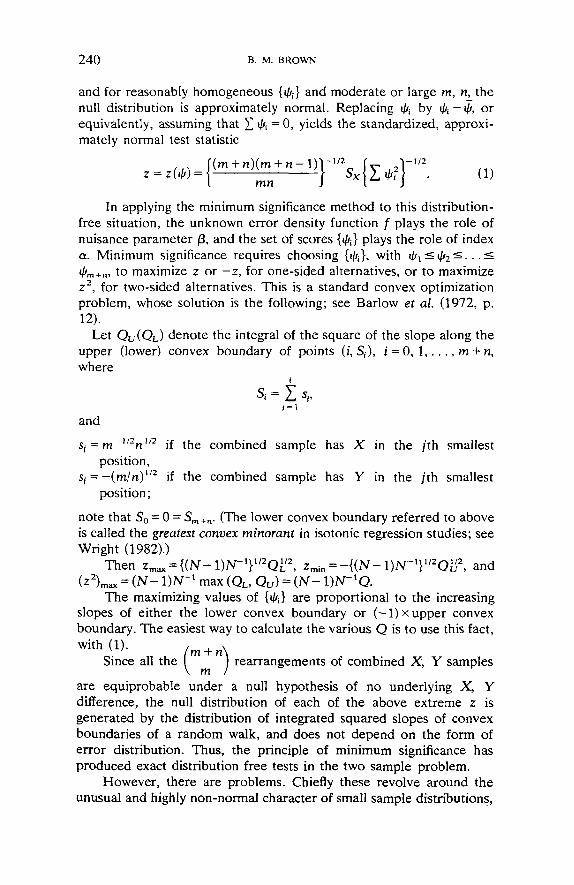
and for reasonably homogeneous {+i} and moderate or large rn, n, the null distribution is approximately normal. Replacing +hi by I,$ - 6, or equivalently, assuming that 1 I+!J~ = 0, yields the standardized, approximately normal test statistic

In applying the minimum significance method to this distribution- free situation, the unknown error density function f plays the role of nuisance parameter p, and the set of scores {ILi} plays the role of index a. Minimum significance requires choosing {+hi), with 5 Jl2’. . .5 +,+,, to maximize z or -z, for one-sided alternatives, or to maximize z2 , for two-sided alternatives. This is a standard convex optimization problem, whose solution is the following; see Barlow et al. (1972, p. 12).

Let Q U ( Q L ) denote the integral of the square of the slope along the upper (lower) convex boundary of points (i, Si), i = 0, 1, . . . , m -I- n, where

i = l

and

si = m-”* n ”* if t he combined sample has X in t h e jth smallest

si =-(m/n)’I2 if the combined sample has Y in the jth smallest

note that So = 0 = S,,,. (The lower convex boundary referred to above is called the greatest convex minorant in isotonic regression studies; see Wright (1982))

Then z,, = {(N- 1)N-’}”ZQL’2, zmin = -{(N- 1)N-’}1’2QZ2, and (z2),,,== (N- 1)W’ max (QL, Qv) = (N- l)N-’Q.

The maximizing values of {&} are proportional to the increasing slopes of either the lower convex boundary or (- 1) x upper convex boundary. The easiest way to calculate the various Q is to use this fact,

position,

position ;

m + n with (1). Since all the ( ) rearrangements of combined X, Y samples

are equiprobable under a null hypothesis of no underlying X, Y difference, the null distribution of each of the above extreme z is generated by the distribution of integrated squared slopes of convex boundaries of a random walk, and does not depend on the form of error distribution. Thus, the principle of minimum significance has produced exact distribution free tests in the two sample problem.

However, there are problems. Chiefly these revolve around the unusual and highly non-normal character of small sample distributions,

MlNlMUhl SIGNIFICANCE A N D DISTRIBUTION FREE TESTS 24 1

difficulties in enumerating the exact small-sample distributions and the existence of a different version for each rn, n combination, and questions of efficiency relative to standard tests. All are discussed in Section 4.

3. One-Sample Tests

In a distribution-free context, the one-sample problem becomes the symmetric location parameter problem, where observations XI , . . . , X , are distributed symmetrically about an unknown location parameter 8. A test of 8 = 8' based on

i = I

(where si = sgn (x i - O'), Gi is a (non-decreasing) function of rank ( / x i - # I ) , +b i i0 ) is distribution free since by hypothesis the {si} equal *l with probabilities f, 4, and are independent of each other and of the {(+}. The null mean and variance of S are 0 and 1 + f , and a convenient normal annroximation refers

to tables of N ( 0 , 1). The principle of minimal significance chooses scores {+[}, with

0 5 4l 5 IL25. . .I +!I,,, to maximize z or -z for one-sided alternatives, or to maximize z 2 for two-sided alternatives. (With this formulation, s, is the sign of the ith smallest absolute residual IX- 81.) Again this is a standard convex optimization problem, with the following solution.

Let QL(Qu) denote the integral of the slope-squared along that part of the lower (upper) convex boundary of the points (i, Si), i = 0, 1, . . . , n, which has positive (negative) slope, where

' s, = c sj.

j = l

If the convex boundary never has positive (negative) slope, then Q L ( Q U ) is {slope x (square-root of length)} for the last, linear section of the boundary with maximum (minimum) slope.

Then t,, = a:", zmin = -a:", and (z2), , = max (QL, a,), = Q. As before, the maximizing {t,hi} are slopes of the relevant convex boundary.

Since under the null hypothesis all 2" sign combinations of {si} are equi-probable, the null distribution of each of the above maximal z is generated by integrals of squares of slopes of convex boundaries of a random walk, and is distribution free.

Calculating the exact small sample distributions requires enumera- tion all of 2" possible random walks {Si}. This problem is not as severe

242 6. M. BROWN

as for the corresponding two-sample problem, but nevertheless grows rapidly in size as n increases. Other difficulties, as for the two-sample problem, are discussed in Section 4.

4. Difficulties

The tests described have exact null distributions, but there are problems in computing these distributions and enumerating the great number of them that seem to be required. Nor do large sample approximations seem to hold much promise; asymptotic distributions appear not to exist. In technical terms, the reason seems to be that the functional (integral of square of slope of lower convex boundary) is not continuous, with respect to the usual uniform distance topology, o n a Brownian motion process. Table 1 gives some critical values for finite sample sizes; they appear not to converge as n ---* m.

TABLE 1

problem : see Section 3. Upper quantiles for distributions of Qu, and Q in the symmetric one-sample

Distribution and quantile level Qu Q Qg Qu Q Qu Q QU Q Qu

n 0.995 0.99 0.99 0.975 n.95 0.95 0 .9 0 .9 n.8 0.8

6 6 6 6 5 8 7 7 6 5

i n 7 7 6.667 5 12 8 8 7 5.833 14 8 8 7.333 6 16 8 8 7.5 6 16* 9 9 7.833 6.372

(8.000) 25* 9.369 9.4 8.4 6.778

100* 12.004 12.125 10.6 8.713 (in.000)

(20.000)

5 5 5 5.833 6 6 6.4

6.8

8.768

~ ~~

4 4 3 3 2 4.5 4.5 3.333 3.333 2.286 4 4 3.667 3.667 2.667 5 5 4 4 2.8 5 5 1 4 3 5 5 4 4 3 5 5 4 4 3

5.611 5.667 4 5 3 2 4.476 3.2

7.25 7.301 5.776 5.8 4.2

* Estimated from random sampling, sample size in parentheses. The I -& points of Q and the 1-28 points of QU appear to be very similar.

Another untoward feature is the presence of some relatively large discontinuities in the exact small sample distributions, whose mag- nitude -0 fairly slowly. Square roots of integer values are a case in point: the effect can be seen in Table 1.

It is plausible that the best way of executing these tests is to estimate exact significance levels through simulation. A computer routine to construct the observed random walk, and find the approp- riate convex boundary and its integrated squared slope, is needed. This


could then be applied to a much larger number of randomly generated random walks to simulate the exact null distribution and hence estimate the observed significance level. Such a sampling procedure was used in Table 1 to estimate values for larger n.

The procedures described are for tests. But to be a serious candidate for use in real-life statistics, allied procedures for estimation and confidence intervals should be available. Here, real difficulties present themselves. It seems that estimates of location, or location shift should be defined as making equal upper and I.ower one-sided significance levels. There seems no alternative but to find these estimates numeri- cally, which involves re-iterating the test procedure with trial parameter values.

It is possible that the equal upper and lower significance levels produced by estimation are both still small. This would provide evidence against the original model, in favour of heteroscedasticity in the two-sample case, and lack of symmetry in the one-sample case. In other words, a goodness-of-fit test is available as a by-product. But this feature is a two-edged sword: it arises because of the strange fact that upper and lower one-sided tests do not use the same test statistic, and it confuses the question of exactly how confidence intervals should be formed.

Large sample distributions associated with estimates and tests are all non-normal, of a rather unusual form. Whether this matters in principle is arguable, but it is certainly inconvenient. For instance, the assessment of efficiency is made difficult: just how efficiency should be measured is not at all clear. It is plausible that the proposed tests have good all-round efficiency for a variety of error-distributions, while perhaps not being fully efficient at any particular one. But how this claim can be verified remains to be seen.

5. Other Analyses

The given tests can be extended to cover other analyses such as simple linear regression and the k-sample problem, or one-way analysis, although in the latter case the distributional difficulties discussed in Section 4 are compounded severely.

First consider investigation of slope in simple linear regression. Observations are (x,, yi) assumed to follow the model yi = Q + pxi + E ~ ,

i = 1,. . . , n, where slope is p and errors {q} have identical distributions. A general method for distribution-free testing of p uses test statistic

where the {bi} are a non-decreasing function of the residuals yi - 0'3,

244 B. M. BROWN

or of their ranks (see Brown and Maritz, 1983). For moderate or large n, the null distribution of S is approximately normal with mean nT& and variance (n - l)-'SxxSw, using the notation S,, = C (ai - 6)(bi - 6). The minimum significance principle chooses scores 4, 5 IJ12 5 - . * 5 IJI,,, which without losing generality sum to zero, in order to maximize (minimize) the standardized stat istic

where x(,) is the design point x, associated with the jth smallest residual y, - p'x,. The situation now is exactly as for the two-sample problem as in Section 2, except that the constants {sl} there now become {x(,)}. An example is given in Section 6.

Now consider the k-sample problem, where observations {yll} are assumed to follow the model

y l , = p + A ~ , + ~ , I , j = l , . . . , n,, i = l , . . . , k, N = x n , ,

with all { E , , } being identically distributed, A 2 0 , and for convenience T; np, = 0, x n,a: = 1. The distribution free approach to testing equal means, i.e. A = 0 against A >0, assigns scores 4 , s IJ12 5. . . s GN to observations in the combined ordered sample, and forms the sums of scores V,, . . . , v k i n the various samples. If 1 $, = 0, as may be assumed, then the test st at ist ic

T = (N- 1) (1 +;)-I( n;' Vf)

is referred to a xf-, distribution. The best-known example of this procedure is the Kruskal-Wallis test when {Gi } are generated by ranks.

Minimum significance requires {IJIi} to be chosen to maximize T. This task is greatly aided by noting that the form of T itself is the result of applying minimum significance to another problem. Specific- ally, suppose that the nuisance vector a = (a,, . . . , q ) in the testing problem A = 0 against A > 0 is known. Let y = Xi yii. A natural linear test statistic is C AiV,, with C niAi = 0; choosing (A,, . . . , hk) for maximum efficiency, i.e. maximum ratio of (non-null mean)' to variance yields hi = ai, and test statistic 1 qUi . Its natural distribution-free modification is 1 qV,. Now apply minimum significance; choose (Y to maximize x aiV, subject to C %ai =0, 1 qa:= 1. The result is ai = (n;' Vi)(ci n;'V;)-1/2, and test statistic

(const). (C n ; ' ~ ; ) .

Express this by saying that a is an ANOVA solution for IJI (since the scores {&} determine the { V,}). On the other hand express the solution JI t o the problem of maximizing (1 siJli)(C IJI?)-"' (see Sections 2, 3) by saying is a convex boundary solution (CBS) for (s,, . . . , s,,). Now subject to the restrictions 1';" Gi = 0, 17 4; = 1, 1: qa, = 0, 1: nia? = 1,


we wish to find

= max max ( c cxi vi). u 4b

Thus cx is an ANOVA solution for J, and J, is a CBS solution for the collection of n , values a’, n2 values a2,. . . , nk values ctk. This observation suggests an iterative method for maximizing T.

(i) Start with any reasonable scores J,, for example the Kruskal-

( i i ) Find the sample score totals {if,}, and hence the ANOVA solu-

(i i i ) Find the CBS solution J, for these a as described in Section 2,

(iv) Continue until a stable solution is reached.

Wallis rank scores.

tions a, = n;’ Vi, with 1 nicx; = 1.

normalizing to make 1 J,: = 1; then repeat step (ii).

I t seems intuitively that this iterative method should converge to t h e correct solution, since each step improves the value of T, by maximizing over a with J, fixed, and then vice-versa; however, a proof of convergence has yet to be found.

There is a connection between the simple regression and k-sample cases. The design weights { x i } i n (2) can be modified in any monotone fashion, and if thus replaced by bounded weights {h,}, the resulting distribution free procedures are robust to errors in design points and observation errors at large design points: see Brown and Maritz (1 983). Incorporating this possibility into the minimum significance framework leads to maximizing

where GI 4 &I. . . S $,,, h , 5 h2 5. . .< h, corresponding to x1 5 x2 5

. . . s x,,, where h(i) is hi whenever the jth smallest residual is yi - Pa; and where C +hi = 1 hi = 0.

Thus J, is a CBS for h, and h is a CBS for J/. An iterative procedure for finding J, and h is very similar to that for the k-sample problem.

6. Examples

In this Section, very brief examples are presented of all the minimum significance procedures outlined in earlier Sections. In all cases, maximizing JI are found from slopes of convex boundaries of random walks. Illustrative graphs (Figures 1-4) do not show vertical scale because all procedures are invariant to scale changes in {qb}.

246 8. M. BROWN

Fig. 1.-Two-sample problem (rn = 4, n = 6) .

(i) Two sample problem. Let m = 4, n = 6 and suppose the combined, ordered X, Y sample is

Y Y x Y Y Y x Y x x. The resulting random walk is shown in Figure 1. Maximizing $ values are proportional to slopes of lower convex boundary; and yield z,,, = (69)”2/4 = 2.0767 (for testing 8 = 0 against 8 > 0). The exact significance level is 04952.

(ii) One sample problem. Suppose that a sample of n = 15 observations, ordered by absolute values, is -0.1, 0.49, 0-49, -0.56, 0.57, -0.59, 4 - 6 1 , -66, 0.70, 0.86, 1-02, -1.11, 1.13, 1.17 and 1.18. The resulting random walk is shown in Figure 2; maximizing t,h values are proportional to slopes of lower convex boundary, and yield z,,,= 2.1909. The exact significance level, for testing 0 = 0 against 8 >0, is 0.0640.

(iii) Linear regression. Suppose that n = 8 pairs of points are

x 2.8 5.2 7.9 9.2 11.7 12.4 14-3 18.3 y 0.81 2.27 2.04 2.81 4.76 3.23 5.36 5.66

Consider estimation of slope 0; the slope which equates significance of upper and lower tail tests (“equates” means slope at which the difference changes sign) is the slope joining the two end points,

Fig. 2.-One-sampIe problem (n = 15).

MINIMUM SIGNIFICANCE A N D DISTRIBUTION FREE TESTS 247

p:' = (5-66-0.81)/(18-3 -2.8) = 0-3129. The two random walks, for p just <p:k and just >p':, are shown in Figure 3, with upper and lower convex boundaries also shown. The Q-values for the two cases are:

(iv) k-sample problem. Suppose that three samples, of sizes 3, 4, 3 and labelled a, b, c, when ordered yield a b a c b a c b b c. Initially, use scores a,, a?, a ) based on rank-averages, and normalized so that 1 n,a, = 0, 1 n,az = 1. This yields a t = -0.4637, a2 = 0.1070, a3 = 0.3210, and a random walk similar to the one shown in Figure 4. The slopes of its lower convex boundary provide the ordered {$,}. Iterating as described in Section 5 yields the final solution a , = -0.4475 a2 = 0.0685 cyJ = 0.3561 with random walk as in Figure 4, and maximum 1 a,V, ={I c ~ f } ' ' ~ = 0.5760.

random walk

convex boundaries

------ convex .-.-.-.- a'ternatives . . . . . . . . . . . . . . random

for p< p*: walk boundaries

Fig. 3.-Simple linear regression (n = 8).

248 B. M. BROWN

Fig. 4.-k-sample problem (k = 3 ; n , = 3, n2 = 4, n3 = 3)

7. summary

The procedures presented are exact, distribution free, and have had the choice of arbitrary score function eliminated by use of a simple principle; minimum significance. Against this, distributional problems, outlined in Section 4, create some practical difficulties.

There are yet more questions of a theoretical nature, concerning the large sample behaviour of the procedures, and the questions of robustness and efficiency, which need resolving before anything of practical use is attempted. However, the present material may provide a first step.

References

BARLOW. R. E., BARTHOLOMEW, D. J., BREMNER, J. M. and BRUNK, H. D. (1972). Statistical Inference Under Order Restrictions. Wiley, New York.

Austral. J. Statist. 24, 3 18-33 1.

Statist. 10. 218-286.

BROWN, B. M. and MAR^, J. S. (1982). Distribution-free methods in regression.

WRIGHT, F. T. (1982). Monotone regression estimates for grouped observations. Ann.

minimum significance and distribution free tests

Documents