NTIA Report 85-171

Millimeter-Wave Propagation in Moist Air:Model Versus Path Data

H. J. LiebeK. C. Allen

G. R. HandR. H. Espeland

E. J. Violette

u.s. DEPARTMENT OF COMMERCEMalcolm Baldrige, Secretary

David J. Markey, Assistant Secretaryfor Communications and Information

March 1985

TABLE OF CONTENTS

LIST OF FIGURES

LIST OF TABLES

LIST OF SYMBOLS

ABSTRACT

1. INTRODUCTION

2. MILLIMETER-WAVE CHARACTERISTICS OF MOIST AIR

2.1 The Propagation Model MPM

2.1.1 Local Line Absorption and Dispersion

2.1.2 Continuum Spectra for Air

2.1.3 Hydrosol Continuum (Haze and Fog)

2.2 Atmospheric Turbulence2.3 Multipath Fading

3. BOULDER LOS EXPERIMENT

3.1 Link Description (27-km Path)

3.2 Data Acquisition3.3 Calibration Procedure (O.l-km Path)

4. OBSERVATIONS, PREDICTIONS, AND RESULTS

4.1 Received Amplitude Levels

4.2 Predicted Responses4.3 Model-Versus-Reported Data

4.4 Boulder LOS Results

4.4.1 Water Vapor Attenuation4.4.2 Turbulence Properties

5. CONCLUSIONS

ACKNOWLEDGMENT

6. REFERENCES

iii

PAGE

iv

vivi i

1

1

3

4

6

7

9

11

16

17

19

21

2124

24

31

35

46

46

46

50

50

52

FIGURE

1

LIST OF FIGURES

Predicted (MPM) specific attenuation a and dispersive delay ~

up to 1000 GHz for moist sea level air and pure water vapor

each for two conditions v = 1 and 30.3(100%RH) g/m3 at T = 30°C

2 Predicted specific attenuation a and dispersive delay ~ for

moist air (0-100%RH) at sea level including simulated fog

conditions (w = 0.1) with roughly 300 m visibility. Five

atmospheric millimeter wave window ranges are marked WI to W5:

a) T = 5°C and w = 0.1.b) T =25°C d 0an w = ..

..... 12

1314

3 Terrain profile of 27.2-km Boulder path with two ray paths for

normal (k =1.34) and subrefractive (k = 0.29) propagation ..... 20

4 Schematic of data acquisition at RX ....... 23

5 Typical daily records of received signal levels sl~2,3 andsupporting meteorological data for Boulder LOS link (L = 27.2 km)taken at a sampling rate, t = ls:

a) relatively quiet atmosphere (lldryll scintillations) 26b) relatively active atmosphere (ll mo istll scintillations) 27c) possible multipath event. . . . . . . . . . . 28d) rai n event. . . . . . . . . . . . . . . . . . . . .. 30

6 Predicted specific attenuation a for humid air and temperatures

every 10°C ranging from 0° to 40°C at the three frequencies f1,2,3of the Boul der propagati on path . . . . . . . . 32

7 Water vapor attenuation slope g = [a(v) - a(O)]/v as afunction of temperature (solid curves are v = const., dashed

curves are RH = const.) at different frequencies:

a) Boulder LOS link frequencies .b) H20 line center frequencies .c) atmospheric transmission window frequencies

iv

333434

FIGURE

8

9

Specific attenuation a and refractive dispersion ~N = N' (f2) - N' (f2)

for humid air and temperatures every 100 e ranging from 0° to 400 e

at two frequencies f1,2 of a Tokyo, Japan, propagation path

Specific attenuation a for humid air at T = 16° ± 2°e and a frequency

of 337 GHz. . . . .. .... . ....

· . 38

· . 40

10 Attenuation rates a at 94 GHz and optical frequencies (visible light)

as functions of absolute humidity v and relative humidity RH••• · . 41

11 Water vapor attenuation rates a(v) across the atmospheric window

range W4 at two temperatures, 5° and -100 e 42

12 Water vapor attenuation rates a(v) across the atmospheric window

ranges W5 and W6 at two temperatures, 8.5° and 25.5°e . . .. . ... 43

13 Water vapor attenuation rate a(v) at 28.8 and 96.1 GHz for a

temperature range between -10° and 400 e . . . . . . . . . . . .. 47

14 Power spectral density W(w) and ratios W2/W1 for event time series

shown in Figure 5:

a) see Figure 5a.b) see Figure 5b.c) see Figure 5c.d) Test of FFT..

v

48484949

LIST OF TABLES

TABLE Page1 Characteristic Tirite and!Horizontal Scales of Atmospheric Processes. . 2

2 Spectroscopic Coefficie.nts of Air Due to Oxygen and Water Vapor Lines

up to 1000 GHz(Local Line Base) . . . .. 8

3 Haze and Fog Attenuation aw and Delay ~w Normalized to w = 1 g/m3 .... 10

4 Performance Parameters for Boul der LOS Link . . . . ...... 22

5 Predicted Specific Attenuation a (dB/km) for a Total PressureP = 101.3 kPa and Hydrosol Attenuation Factor Xw at Various RelativeHumidities RH (%) and Temperatures T(K) for Selected Millimeter-waveFrequencies .. 36

6 Overview of Experimental Results From Horizontal Line-of-Sight (LOS)

Paths, a Mountain Peak Zenith (ZEN) Path, and Laboratory (LAB)Experiments, All Used As Corroborative Data for the PropagationProgram MPM . . . . . . . . . . . . . . . . . . . .. ... 37

7 Summary of an MPM-Analysis of Atmospheric Brightness T~ Measured atFrequencies Between 2.5 and 90 GHz from a Mountain Peak 45

vi

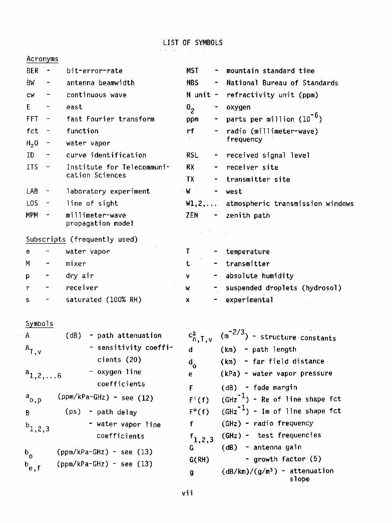
LIST OF SYMBOLS

N unit - refractivity unit (ppm)

W1,2, ... atmospheric transmission windowsZEN zenith path

Acronyms

BER ­

BWcw

E

FFT ­

fct ­H2 0 ­

ID

ITS -

LAB ­

LOS ­

MPM -

bit-error-rate

antenna beamwidth

continuous wave

east

fast Fourier transform

function

water vapor

curve identification

Institute for Telecommuni­cation Sciences

laboratory experiment

line of sight

millimeter-wavepropagation model

MST

NBS

O2ppm

rf

RSL

RXTXW

- mountain standard time

- National Bureau of Standards

oxygen

- parts per million (10-6)

radio (millimeter-wave)frequency

received signal level

receiver site

transmitter site

- west

T temperature

t transmitter

v absolute humidity

w suspended droplets (hydrosol)x experimental

Subscripts (frequently used)

e water vapor

M mixer

p dry air

r receiver

s saturated (100% RH)

Symbols

A (dB) - path attenuation c2 (m- 2/3 ) - structure constantsn,T,vA - sensitivity coeffi- d (km) path lengthT,v

cients (20) do (km) - far field distancea - oxygen line e ( kPa) water vapor pressure1,2, ... 6

coeffi ci ents F (dB) - fade margina (ppm/kPa-GHz) - see (12) F' (f) (GHz-1) - Re of line shape fcto,p

B (ps) - path delay Pl(f) (GHz-1) - 1m of line shape fct

b - water vapor line f (GHz) - radio frequency1,2,3

(GHz) - test frequenci escoefficients f1,2,3

bo (ppm/kPa-GHz) - (13) G (dB) - antenna gainsee

b (ppm/kPa-GHz) - (13) G(RH) - growth factor (5)e,f see

g (dB/km)/(g/m3 ) - attenuationslope

vii

Symbols continued

- specific attenuation

- specific delay

- refractive delay (No)- line width- small change

bandwidth- overlap correction

- dielectric constantof water

- antenna efficiencyfactor

a(t) (dB/km)

f3( f) (ps/km)

~o (ps/km)y (GHz)

A

Af (MHz)

6

t = (2+E 1 )h" - see (14)

~

6 =300/T(K) relative inversetemperature

A (mm) - wavelength

"0 (GHz) - line center frequencya (ppm2) - variance of N

as (dB2) - variance of st (s) - sampling rate

t w (ns) - water relaxationtime constant

w (Hz) - fluctuation frequencyWo (Hz) - corner frequency

(km) - initial height

(dB) - free space loss

(dB) - insertion loss

- effective Earth radius(Fi g. 3)

(m) turbulence scale sizes

(ppm) - complex refractivity(ppm) - refractivity(ppm) - refractive dispersion

(ppm) - extinction

- integer

- line number (7)

(mW) - rf power

(kPa) - barometric pressure(kPa) - dry air pressure

(dBm) - receiver noise level(mm/hr)- rain rate

(%) - relative humidity

(kHz) - line strength

(dB) - system gain

(dB) - log-amplitude RSL(Oe) - temperature

(K) - effect. receivernoise temperature

(s) - time(m/s) - cross-wind speed

(mm) - path-integratedwater vapor

Q.1,0

N

NON' (f)

N"(f)

n

na,bPtP

p

QrR

RH

S

Sys1,2,3T

TE

t

v (g/m 3 ) - absolute humidity

W(w) (dB2/Hz) - power spectraldensity

w (g/m3 ) - hydrosolconcentration

wo

(g/m3 )

x (km)- :: w(RH = 0%)- path distance

- hydrosol factor

viii

MILLIMETER-WAVE PROPAGATION IN MOIST AIR:MODEL VERSUS PATH DATA

H. J. Liebe, K. C. Allen, G. R. Hand, R. H. Espeland, and E. J. Violette*

A practical atmospheric millimeter-wave propagation model (MPM)is updated and tested with experimental data from horizontal, line­of-sight links when there is no precipitation. The MPM computerprogram predicts attenuation and delay properties of moist air overranges in frequency from 1 to 1000 GHz and in height from 0 to 30 km.Input variables are radio path distributions of pressure, temperature,relative humidity, and a suspended droplet concentration simulatinghaze and fog conditions. Terrestrial path data from millimeter-wavepropagation experiments, including those from a 27 km link operatedat 11.4, 28.8, and 96.1 GHz by the Institute for TelecommunicationSciences (ITS), have been analyzed. Calibrated mean signal levelspermitted studies of water vapor losses. In addition, a spectralanalysis was performed of clear-air scintillations caused by turbu­lence. In general, good agreement is obtained with the MPM for testfrequencies up to 430 GHz.

Key words: atmospheric attenuation and delay; millimeter wave propertiesof moist air; propagation program MPM; terrestrial radio path data

1. INTRODUCTION

Atmospheric propagation limitations dominate most considerations in the advance­

ment of millimeter-wave applications (Crane, 1981; Bohlander et al., 1985). Adverse

weather causes millimeter-wave signal degradations due to rain, wet snow, suspended

particles, and water vapor. A propagation model provides a cost-effective means of

predicting the performance of a system for its intended use by considering limiting

factors of the atmosphere that in the actual operating environment may be difficult

to identify. The Institute for Telecommunication Sciences (ITS) has developed a

modular Millimeter-wave Propagation Model labeled MPM (Allen and Liebe, 1983; Liebe,

1983). Based on meteorological variables, the model predicts propagation effects

(that is, radio path attenuation, delay, and medium noise) for a radio path through

the first 100 km (nominally ground-to-space) of the atmosphere. Frequencies up to

1000 GHz (1 THz) are considered. The model has been used, for example, to provide

estimates of millimeter-wave, average-year attenuation distributions for diverse

climates across the United States (Allen et al., 1983).

This report addresses the moist air portion of the MPM. Central to the modelare more than 450 spectroscopic parameters describing local «1 THz) absorption

lines of the molecules O2 and H20 complemented by' continuum spectra for dry air,

*The authors are with the Institute for Telecommunication Sciences, NationalTelecommunications and Information Administration, U. S. Dep~rtment of Commerce,325 Broadway, Boulder, Colorado 80303.

water vapor, and hydrosols (i.e., suspended water droplets for haze and fog condi­

tions). Laboratory measurements of absolute attenuation rates at 138 GHz for simu­

lated air with water vapor pressures up to saturation led to an improved water vapor

continuum (Liebe, 1984). In addition, other research findings have been reported

recently on the spectroscopic data base, which impact predictions and thus warranted

an update (Liebe, 1985) of earlier versions (Waters, 1976; Liebe, 1981). The new

MPM describes millimeter-wave characteristics of moist air and is presented in

Section 2.1 in the form of a comprehensive complex refractivity N.

Terrestrial propagation experiments in the 10 to 100 GHz range have been con­

ducted by ITS over path lengths between 0.1 and 27 km employing cw and broadband

(>1 GHz) signals (Violette et al., 1983; Espeland et al., 1984). In order to com­

pare MPM predictions with realistic data, absolute intensity measurements were per­

formed of phase-coherent signals at 11.4, 28.8, and 96.1 GHz over a 27.2 km path

located in Boulder, Colorado. Calibrated levels of received signal amplitudes have

been processed for time periods free of precipitation to obtain mean values s(dB)

and variances us(dB2) as indicators for atmospheric losses and fluctuations intro­

duced by water vapor, turbulence, and possible layering effects. Attenuation (dB/km)

measurements have been made at 28.8 and 96.1 GHz when the atmosphere was well mixed.

Natural atmospheric fluctuations in density and composition cause variations in

the refractivity N±~N on various time and space scales outlined in Table 1.Turbulence-induced variability ~N serves to explain temporal and spatial fluctu-ations in received signal amplitudes, phases, and angles-of-arrival. Turbulence

models addressing amplitude scintillations of millimeter waves are discussed brieflyin Section 2.2.

Table 1. Characteristic Time and Horizontal Scales ofAtmospheric Processes (Orlanski, 1975)

Process

Turbulence

Earth rotation

Weather systems

Seasonal changes

Weather cycles

Approximate Time Scale Approximate Horizontal Scale

s (mi 11 i sec. to m10-2-104 hours) 10-3-103 (micro)

105 (day) 103-104 (meso)105-106 (week) 104-105 (synoptic)106-107 (month) 105-106 (macro)107-109 (year) 106-107 (global)

2

Experimental data capable of substantiating these models have been limited to a few

cases (e.g., Cole et al., 1978; Filho et al., 1983; Vogel et al., 1984). Scintilla­

tion results obtained with the Boulder link for a frequency ratio of 1:8.4, add suit­

able test data. Section 2.3 touches upon the problem that weak turbulence might

sustain large-scale refractive index stratifications. Such conditions might result

in deep fade events since stable layering can lead to multiple rays that mutually

interfere.

Details of the ITS terrestrial propagation experiment are summarized in Sec­

tion 3. Observations of received signal strengths obtained with this link, together

with simultaneously measured meteorological data, are presented in Section 4. Also

included are selected data up to 430 GHz that have been reported in the literature.

Section 5 contains the results of various intercomparisons between tractable propa­

gation data from individual events and model results. The report concludes with a

discussion of the validity of predictions and their value in forecasting the perform­ance of millimeter wave systems operating through the atmosphere.

2. MILLIMETER-WAVE CHARACTERISTICS OF MOIST AIR

Millimeter waves traversing an atmosphericline-of-sight (LOS) path lose energy

in various ways, most of which are frequency-dependent. Radiated energy can be ab­

sorbed, scattered out of the path, or diverted by refraction and diffraction effects

that cause the signal either to miss the receiving antenna and/or to arrive out of

phase with the main ray. All these interactions are dynamic in nature, driven bythe variable atmosphere and leading to modulations of the propagating radio wave in

amplitude and phase (transit time).

Two basic approaches for predicting transmission ch.aracteristics of moist air

are taken:

Physical Model (Section 2.1). Number concentrations of absorbers, refractive

layers, and diffraction boundaries as part of the path geometry, all are

accounted for based on physical quantities measurable, at least in principle,

at any given path location and time.The transmission of broadband (>100 MHz) signals adds the additional dimensionof frequency response across the signal bandwidth. In digital schemes, disper­

sive group delay within the atmospheric propagation channel can cause inter­

symbol interference limiting the maximum data transmission rate. For example,

100 megabit per sec (Mb/s) tolerate about 3 ns deviations from frequency-linear

behavior across the bandwidth with no increase in bit error rate (BER).

3

Statistical Models (Sections 2.2 and 2.3). Time series of received signal level

(RSL) are analyzed in conjunction with meteorological data over time intervals

of events specified in Table 1. The RSL is treated as a random variable, dis­

regarding the physical origin of the variability. Typically, a median value is

defined over a reference period (e.g., 1 h) superimposed by short-term fluc­

tuations and both processes are evaluated statistically.

2.1 The Propagation Model MPM

The computer program MPM is a physical model developed for applications in tele­

communications, radio astronomy, remote sensing, etc., within the 1 to 1000 GHz range

(Liebe, 1981; 1985). Radio path behavior through a moist atmosphere is described by

cumulative path attenuation

d

A = !ex(X)dX

o

dB (la)

(lb)ps,

and by path delayd

B = f~(X)dXo

where dx is an increment of the path length x in kilometers (km) which is of total

length d. Attenuation A quantifies the amount of energy extracted from a plane wave

propagating through the atmosphere, delay ~ is a measure of the excess traveling

time with reference to vacuum. Specific power attenuation ex and propagation delay ~

can be expressed in the form

ex = 0.1820f W1(f) dB/km (2a)

and

ps/km, (2b)

where frequency f is in gigahertz (GHz) throughout. The heart of the model is a

macroscopic measure of interactions between radiation and the propagation medium,

expressed as complex refractivity in N units (10- 6 =ppm)

N = N + N' (f) + J·N"(f)o • (3)

4

The refractivity consists of a frequency-independent term No plus various spectra of

refractive dispersion NI (f) and absorption Nil (f).

Meteorological Parameters

Gaseous oxygen (02) and water vapor (H20),and suspended water droplets are

considered to be the principal absorbers. The physical state of air is described by

four measurables P-T-RH-w, which relate to internal model variables p-a-e(v)-wo as

follows:

T = (300Ia) - 273.15 (OC),P = P + e (kPa),

(%), w =Wo G(RH) (g/m3 ) •

Barometric pressure is labeled P, where p is dry air pressure and e is partial water

vapor pressure, all in units of kilopascal (1 kPa = 10 mb); temperature T in degrees

Celsius (OC) is converted to a relative inverse temperature parameter a, which for Tin absolute Kelvin units equals 300/T(K); and relative humidity

RH = (e/es

)100 = (v/vs)100 = 41.51 e a-5 10(9.834 a - 10) ~ 100% (4)

is given as absolute humidity ratio described interchangeably by either water vapor

partial pressure e or vapor concentration v =7.217 e a (g/m3 ). The subscript "S"

denotes the saturation limit at RH = 100%. A dry mass concentration of hygroscopic

aerosol is Wo in g/m3 and an approximate expression for the unitless mass growth

factor for RH < 96% is given by (Haenel, 1976)

G ~ 1001(100-RH). (5)

Complex Refractivity N

Radio refractivity of air has been measured accurately at microwave frequencies

(e.g., Boudouris, 1963) and reviewed recently (Hill et al., 1982) to be

No = (2.588 p + 2.39 e)a + 41.63 e a2. (6)

Absorption and dispersion spectra are obtained from na =48 oxygen lines,

nb = 30 water vapor lines, and various continuum spectra Np (dry air), Ne (water

vapor), and Nw (hydrosol) via

5

n nbaN"(f) = L: (SF"). + Nil + L (SF II

). + Nil + Nili=l 1 P i 1 e w

and

na nbN' (f) = ~ (SF')i + N' + L: (SF ' ). + N' + N1

~ P 1 e wi=l i

dry air + water vapor + susp. droplets.

(7a)

(7b)

In the line-by-line calculations t S is a line strength in kHz and F' and FII are real-1and imaginary parts of a shape function in GHz . Pressure broadening of the domi-

nant lines leads to two different types of frequency responses t namely sharp reson­ance lines and continuum spectra. Both are treated in the following for atmospheric

conditions up to heights of h = 30 km. Self- and foreign-gas-broadening influences

have to be taken into account. Trace gas spectra are neglected since their abundance

is too small to markedly affect tropospheric propagation.

2.1~1 Local Line Absorption and Dispersion

The Van Vleck-Weisskopf function was modified by Rosenkranz (1975) to describe t

to first order t line overlap effects. This leads to local absorption and dispersionline profiles

c- ("0 - f)o y -(uo + 061(1-) GHz-1FII = + (Ba)

(" - f)2 + y2("0 + f)2 + y2 "

0 0

and

C"- f + y(y + fo)/" "0 + f + y(y - fo)/"o

- L ) GHz-1 .F' = . I 0 + (Bb)(" - f)2 + y2 f)2 + y2(" + "00 0

6

The line parameters are calculated according to the scheme below:

Symbol O2 lines in air H20 lines in air

S , kHz 3 -6 - 8)J b1e83. S exp[b2(1 - 8)J (9)a1P8 10 exp[a2(1

, GHz(0.8-a4) -3 b

3(P80.8 + 4.80e8)10- 3 (10)y a3(p8 + 1.le8)10

a6 10-3 0 (11)aSP8

Line center frequencies Vo and the spectroscopic coefficients a1 to a6 , b1 to b3 for

strength S, width y, and overlap correction 0 are listed in Table 2.

Standard line shapes FII(f), including the Van Vleck-Weisskopf function (8),

predict in frequency regions of local line dominance about the same results for

NII(f) as long as FII(f) values are larger than 0.1 percent the peak value at f =vo

Wing contributions that are less than 0.1 percent depend upon the chosen line shape

function. Far-wing contributions « 0.001 percent) differ by as much as 1:80

(Liebe, 1984). No line shape has been confirmed that predicts absorption intensi--3 -6ties over ranges (10 to <10 ) of FII(vo)' as required for the water vapor spec-

trum. Expected far-wing contributions from strong (> 106 dB/km) infrared lines are

accounted for summarily by empirical correction.

2.1.2 Continuum Spectrum for Air

Continuum spectra in (7) identify dry air and water vapor terms Np + Ne and

must be added to the selected group of local O2 and H20 resonance lines (Table 2)

described by (8) in order to correctly predict atmospheric millimeter wave attenua­

tion in window ranges between lines. Continuum absorption increases monotonically

with frequency.

The dry air continuum

and

N"(f) = 1(2a {y [1 + (fly )2 J[1 + (f/60)2 J}-1 + p ap If p 82P 000

7

(12a)

(12b)

Table 2. Spectroscopic Coefficients of Air Due to Oxygen and Water Vapor LinesUp to 1000 GHz (Local Line Base)

"vo a, aZ a3a4 a5 a6 "V b, bZ ~-- 0

8Hz (Hz/kPa)/1 0- 3 MHz/kPa lO-3/ kPa GHz kHz/kPa t1Hz/ kPa

49.452379 0.12 11.830 8.40 0 5.60 1.7 22.235080 0.1090 2.143 27.8449.962257 0.34 10.720 8.50 0 5.60 1.7 67.813960 0.0011 8.730 27.6050.474238 0.94 9.690 8.60 0 5.60 1.7 119.995940 0.0007 8.347 27.0050.987748 2.46 8.690 8.70 0 5.50 1.7 183.310117 2.3000 0.653 28.3551.503350 6.08 7.740 8.90 0 5.60 1.8 321.225644 0.0464 6.156 21.4052.021409 14.14 6.840 9.20 0 5.50 1.8 325.152919 1.5400 1.515 27.0052.542393 31.02 6.000 9.40 0 5.70 1.8 336.187000 0.0010 9.802 26.5053.066906 64.10 5.220 9.70 0 5.30 1.9 380.197372 11.9000 1.018 27.6053.595748 124.70 4.480 10.00 0 5.40 1.8 390.134508 0.0044 7.318 19.0054.129999 228.00 3.810 10.20 0 4.80 2.0 437.346667 0.0637 5.015 13.7054.671157 391.80 3.190 10.50 0 4.80 1.9 439.150812 0.9210 3.561 16.4055.221365 631.60 2.620 10.79 0 4.17 2.1 443.018295 0.1940 5.015 14.4055.783800 953.50 2.115 11.10 0 3.75 2.1 448.001075 10.6000 1.370 23.8056.264777 548.90 0.010 16.46 0 7.74 0.9 470.888947 0.3300 3.561 18.2056.363387 1344.00 1.655 11.44 0 2.97 2.3 474.689127 1. 2800 2.342 19.8056.968180 1763.00 1.255 11.81 0 2.12 2.5 488.491133 0.2530 2.814 24.9057.612481 2141.00 0.910 12.21 0 0.94 3.7 503.568532 0.0374 6.693 11.5058.323874 2386.00 0.621 12.66 0 -0.55 -3.1 504.482692 0.0125 6.693 11.9058.446589 1457.00 0.079 14.49 0 5.97 0.8 556.936002 510.0000 0.114 30.00

ex> 59.164204 2404.00 0.386 13.19 0 -2.44 0.1 620.700807 5.0900 2.150 22.3059.590982 2112.00 0.207 13.60 0 3.44 0.5 658.006500 0.2740 7.767 30.0060.306057 2124.00 0.207 13.82 0 -4.13 0.7 752.033227 250.0000 0.336 28.6060.434775 2461.00 0.386 12.97 0 1.32 -1.0 841.073593 0.0130 8.113 14.1061.150558 2504.00 0.621 12.48 0 -0.36 5.8 859.865000 0.1330 7.989 28.6061.800152 2298.00 0.910 12.07 0 -1.59 2.9 899.407000 0.0550 7.845 28.6062.411212 1933.00 1.255 11.71 0 -2.66 2.3 902.555000 0.0380 8.360 26.4062.486253 1517.00 0.078 14.68 0 -4.77 0.9 906.205524 0.1830 5.039 23.4062.997974 1503.00 1.660 11.39 0 -3.34 2.2 916.171582 8.5600 1.369 25.3063.568515 1087.00 2.110 11.08 0 -4.17 2.0 970.315022 9.1600 1.842 24.0064.127764 733.50 2.620 10.78 0 -4.48 2.0 987.926764 138.0000 0.178 28.6064.678900 463.50 3.190 10.50 0 -5.10 1.865.224067 274.80 3.810 10.20 0 -5.10 1.965.764769 153.00 4.480 10.00 0 -5.70 1.866.302088 80.09 5.220 9.70 0 -5.50 1.866.836827 39.46 6.000 9.40 0 -5.90 1.767.369595 18.32 6.840 9.20 0 -5.60 1.867.900862 8.01 7.740 8.90 0 -5.80 1.768.431001 3.30 8.690 8.70 0 -5.70 1.768.960306 1.28 9.690 8.60 0 -5.60 1.769.489021 0.47 10.720 8.50 0 -5.60 1.770.017342 0.16 11.830 8.40 0 -5.60 1.7118.750341 945.00 0.000 15.92 0 -0.44 0.9368:498350 - 67.90 - 0.020- 19.20- - 0.6 - - - 0 - -C-424.763120 638.00 0.011 19.16 0.6 0 1487.249370 235.00 0.011 19.20 0.6 0 1715.393150 99.60 0.089 18.10 0.6 0 1773.838730 671.00 0.079 18.10 0.6 0 1834.145330 180.00 0.079 18.10 0.6 0 1

make a small contribution at ground level pressures due to the nonresonant 02 spec­

trum below 10 GHz and a pressure-induced N2 spectrum, effective above 100 GHz

(Stankevich, 1974). A width parameter for the Debye spectrum of 02 is formulated inaccordance with (10) to be Yo = 5.6 x 10-3(p + 1.le)SO.8 (GHz) (Rosenkranz, 1982).

The continuum coefficients are a = 3.07 X!0-4, (Rosenkranz, 1975), and-10 0 .

a = 1.17 x 10 (Dagg et al., 1982).p

The water vapor continuum

peri mental data in the case of

to

is an empirical contribution derived from fitting ex­

Nil and theoretical data in the case of Nt, which lede e

and

(l3a)

(Bb)

where b = 6.47 x 10-6 (R. Hill, personal communications, 1984),o -6 -5

bf = 1.40 x 10 and be = 5.41 x 10 (Liebe, 1984).

2.1.3 Hydrosol Continuum (Haze and Fog)

Suspended water droplets (hydrosols) in haze and fog (or clouds) are millimeter

wave absorbers. Their size range of radii is below 50 ~m, which allows the Rayleigh

approximation to Mie scattering theory to be used for calculating refractivity con­

tributions Nw to (7) in the form (Liebe, 1981; Falcone et al., 1982)

(l4a)

and

(14b)

where t = (2 + E 1 )h;lI; and E',E II are real and imaginary parts of the dielectric con­

stant for water. For frequencies above 300 GHz, the following approximation

(14c)

9

can be used instead of (14a), based on data reported by Simpson et al. (1979).

The dielectric data ~I ,~II of bulk water are calculated with the Debye model,

which is valid for f ~ 300 GHz as reported by Chang and Wilheit (1979):

(15a)

and

(15b)

-5where t w =4.17 x 10 e exp(7.13 e) ns. Table 3 lists numerical examples of

Ci = 0.182f N" (dB/km) for two temperatures (OOC and 25°C) at selected frequencies.w wA strong temperature dependence can be noticed.

Haze conditions are related to vapor-to-droplet conversion processes reversible

(swelling/shrinking) with relative humidity for values below RH = 100 percent. The

simple growth function (5) provides an approximation of the RH-reversible conversion

up to RH ~ 96 percent. Typical dry air mass loadings of hygroscopic aerosol in

ground level air are below Wo ~ 10-4 g/m3. A practical growth function covering the

range above RH = 96 percent, including the irreversible condition of supersatura­

tion, RH>100 percent, is lacking. Such a function is needed to explain the growth

of suspended droplet concentrations to values w = 10-3 to 1 g/m3 as observed under

various fog conditions. At present, reported values for ware used in (14) and the

contributions are added to respective calculations (7) for saturated (100%RH) air.

Table 3.

Haze and Fog Attenuation CiW

and Delay ~w Normalized to w = 1 g/m3

TEMPERATURE FREQUENCY f (GHz)

T 1 10 30 100 200 300 400 600 800 1000

°C CiW

(dB/km)

0 .0010 .097 .82 5.4 9.3 10.8 13 18 23 29

25 .0005 .051 .45 4.2 10.8 15.3 21 31 40 48

~w (ps/km)0 .69 .32 .09 .04 .04 .04 0 0 0 0

25 .62 .49 .20 .06 .04 .04 0 0 0 0

(14 a,b) (14c)

10

In summary, (1) to (15) constitute the physical MPM, which is capable of pre­

dicting millimeter wave properties of moist air for given sets of P-T-v(RH)-w distri--4 6butions along a radio path. A full range of MPM coverage (i.e., aCf) = 10 to 10

dB/km, ~(f) = ±104 ps/km, f = 1 to 1000 GHz) is exhibited in Figure 1 for two cases

[v = 1 and 30.3(100%RH) g/m3 ] , each for pure water' vapor (H20 self-broadening) and

moist sea level air. Examples in Figure 2 show the humidity dependence of specific

attenuation a and dispersive delay ~ for sea level conditions (P = 101.3 kPa, RH = 0

to 100%, w = 0.1 g/m3 , T = 5 and 25°C) and frequencies up to f = 350 GHz. Five at­

mospheric transmission windows are indicated by WI to W5.

Starting from a given choice of mean atmospheric conditions, it is the fluctua­tions in P-T-v-w that modulate the average moist air refractivity N± ~N(t,x) in

space and time which, in turn, influences the propagating radio wave. To evaluate

the resulting propagation effects, it is necessary to investigate the stochastic

functions that govern atmospheric fluctuations. The practical effects of refractiv­ity N and its variance a are to produce phenomena that may be grouped into those

resulting from small-scale turbulence structures (see Section 2.2) and those from

large-scale structures in the atmosphere, such as diurnal and weather changes, over­

all temperature and water vapor distributions including inversions, etc. The latter

manifest themselves in effects such as ray bending, ducting, propagation delay dis­

persion, and multipath interference (see Section 2.3).

2.2 Atmospheric Turbulence

The theory of wave propagation in a turbulent medium, as described by Tatarski

(1961), was extended to millimeter waves by Clifford and Strohbehn (1970), Ishimaru

(1972), Ott and Thompson (1978), and Hill and Clifford (1981), among others. Sub­

millimeter wave turbulence effects have been treated recently in a review by Bohlander

et al. (1985). Under ideal assumptions that turbulent eddies are distributed within

a propagation path in an isotropic and homogeneous manner, the structure function at

separation ~x can be written as

(16)

where < > denotes ensemble averages, usually replaced by time averages. The separa­tion ~x of two measurement points has to be between an inner scale Q. « 0.01 m) and

1 ~

an outer scale Q (> 5 m), and c2 in units of m- 2/3 is called the refractive struc-o ~ nture constant. This parameter is the key in relating turbulence to propagation ef-

fects such as amplitude scintillations, phase front distortions, and variations in

angle-of-arrival.

11

--- Air-broadened--- Self-broadened (H20)

400 600FREQUENCY, GHz

1000

v(RH)

g/m3

30.3 (100%)30.31.0 (3,3%)1.0

800

Curve ID P

kPa1 101.32 p=O3 101,34 p=O

""a. I'"

................:" "••:::••

1

0)

.. ,,.'" .. ' .. , 4

200

10 6

10~ MPM

E 10 4

~

"- 10 3m"'0

10 2

Z0 10'-I-4: 10 0

::>Z 10-'WI-

10-2I-4:

10-3 :... .-

" ," '

10-4 ' '

0

1000800

"""f

I,""

, '

, """"

I,"", ,

b)

200

log

P = 0

P = 101.3 kPA

• I

:.~~~£1±=-+-tr-~-f-··~log : :: ,.' " :. ... .

. I"'

400 600FREQUENCY, GHz

Predicted (MPM) specific attenuation a (a) and dispersive delay B (b)up to 1000 GHz for moist sea level air (#1 and 3) and pure water vapor(#2 and 4) each for two conditions v = 1 and 30.3 (lOO%RH) 91m3 at T = 30·C(Note the linear-log scales used to display delay S )

E 103

102

~

"- 10(J)

Q. ~O

" -10>- 24: -10_J -10

3

W0 600

W> 100(j)

£!:~OW

0...(j) -100-0

-600

0

Figure 1.

12

SoI

1IxlO, 6 50 1014+--j 7 75 1 049

8 100 10849 10O+w 1 084

v(100%RH)=6.8, w=0.1 g/m 3

Curve 10 RH,% So,ps/km1 ·-0- 9442 1 9453 3 9494 10 9585 25 979

E.::I."­000.

>: 5

~WoW>(j) 0n::wCL -0.2(J)

o

a)100

h - 0 km

E P=101.3 kPa. T== SOC

~ 10 ~~9"-m 't\?"U

't\~....

Z0 1

~\.f- .~::>zw

.1f-f-«

- S oL......a.-&..-..I-...J..-oL-&.....J......lL-1..........'--I-.-..J--�-..L....J.----~............-.........l.-.a......L~3.s......L.0~O--l-~3~5050 100 150 200 250

FREQUENCY, GHz

Figure 2. Predicted specific attenuation a and dispersive delay S for moistair (O-lOO%RH) at sea level including simulated fog conditions(w = Owl) with roughly 300 m visibility. Five atmosoheric milli-meter wave window ranges are marked Wl to W5,(~ =3.336 No' refractive delay):a) T=5°C and w=O.l 0

13

350300

5

4~~~~~~~=;';;;;2;I·3~;;;,;;;=====~·. f3

1 0

100 150 200 250FREQUENCY, GHz

50

v{ 1 OO%RH)=23. a g/m 3

Curve 1D RH,% f3 o ,ps/km

1 a 8802 1 8853 3 8944 1a 9255 25 9916 50 11 027 75 121 28 1 00 1323

.0130

E:;{. 25

"f/JQ.20..

>-«....J 15W0

W 10

>(f)

5a::wa..(J) 0-0

-50

b)100

h - 0 km

EP==101.3 kPa, T==25°C

,:.{.10 ~)"-m

1) ~~..

Z 'i\'\0 1t-«:::>zw

•1J--I-«

Figure 2. continued. b) T =25°C and w=0

14

The propagation experiment described in Section 3 yields time series set) of

log-amplitude behavior at three frequencies f. Under atmospheric conditions where

(16) is valid, the variance of log-amplitude scintillations is expected to be propor­

tional to (Vogel et al., 1984)

a ex:S

(I7)

Also, it is assumed that the transmitting and receiving antenna sizes are small rela­

tive to an approximate 1st Fresnel zone clearance ~, and in turn, the Fresnel zone

is small compared with the outer turbulence scale Qo' The radio wavelength A fol­lows from

A =299.8/f mm. (18)

Since both air density and absolute humidity v affect the refractivity N, the

structure parameter c~ can be expressed in terms of analogous parameters for temper­

ature, humidity, and barometric pressure. Neglecting pressure variations,

c~ is given by

c2 c2 cTvc2 = A2 T_ + A2 v_ + 2ATA

v-= __

n T <T>2 v <V>2 <T><v> -2/3m , (19)

where the sensitivity coefficients AT,v are calculated from the refractivity No (Hilland Clifford, 1981). The last term in (19) can be approximated by

cTv<T><v> [

C2 c2 ] 1/2~ + . v + T= - <V>2 <T>2 . (20)

The positive sign usually applies during the day and the negative sign during the

night, due to a change in the direction of the temperature gradient near the ground.Under some dry conditions (Liebe and Hopponen, 1977), (20) can sUbstantially cancel

the contribution of the other two terms and result in a situation for which the

value of c~ is small (lldry ll scintillations). Frequently, the ground evaporateswater vapor. In these instances, humidity fluctuations will surpass, in relative

terms, temperature fluctuations by far, say

15

and humidity variance dominates the refractivity structure.

are large (ll mo ist ll fluctuations). The structure constant is

est the ground where millimeter-wave values for c2 can range-2/3 n

m

(21)

The resulting c~ valueshighest in layers near­between 10-12 and 10-17

The refractivity N given by (3) is complex. Terms should be added to (17) to

account for contributions from the variance of absorption and the covariance of re­

fraction and absorption (Ott and Thompson, 1978; Hi.ll and Clifford, 1981). Usually,

humidity variations dominate the structure constant c~ via refraction , and the con­

tribution of absorption to fluctuations will be difficult to observe in the milli­

meter-wavelength range, unless specific values of about 5 dB/km are exceeded (Filho

et a1., 1983).

When a wind with average speed u1

(m/s) transverse to the propagation path car­

ries the spatial structure of refractivity fluctuations through the propagation

path, a modulation spectrum of scintillation frequencies w (Hz) is imposed upon the

propagating wave. Between inner and outer scales of turbulence a spatial spectrum

exists which has a theoretical (Kolmogorov) foundation. Turbulence structures

larger than the size of the 1st Fresnel zone produce signal scintillations with con­

stant spectral power density Wo(dB2/Hz). These occur in the lower frequency portion

of the spectrum. The power density falls off rapidly (w- 8/ 3 ) with increasing fre­

quencies w. The spectral asymptotes Wand w- 8/ 3 cross at the IIcornerll frequencyo

Hz. (22)

The spectral power density for the range w » Wo is proportional to (Cole eta1.,1978)

W(w) « f2 c2 d Q~/3n 1

dB2/Hz. (23)

Structure sizes larger than Q are ill-defined in form. Turbulent phenomenaomerge with large-scale variations in the atmosphere. A power spectrum W(w) should

reveal the processes discussed and allow the deduction of a relative refractive struc­

ture constant c~ « Wo(w) and wind speed u1

via (17) and (22).

2.3 Multipath Fading

In some regions of the world, frequency-selective fading phenomena from atmos­

pheric refractive layers are fairly common. They are associated with stable

16

atmospheric conditions (weak turbulence) plus rapid, height-dependent reductions in

water vapor concentration (e.g., fog over moist river valleys during calm, cool

nights, and early mornings of hot, summer weather). Under such conditions a radio

ray can be trapped and channeled in a duct, where the normal spherical spreading

loss Lo (see Section 3) is no longer valid and possible dispersive propagation velo­

cities exist. The result is a strong short-term RSL variability due to more than

one component of the radio field arriving at the receiver by way of separate, slight­

ly differing paths. Occasionally, when only two rays interfere with each other,

both being of similar magnitude, the RSL can behave very erratically, with unpredic­

table deep fades in the range of 20 to 40 dB and serious amplitude distortions across

the propagation channel bandwidth. Mu1tipath effects present problems for the trans­

mission of digital data. Delay spread causes the received symbols to overlap. The

resulting intersymbo1 interference leads to decoding errors. For example, a delay

difference of 3 ns can raise the BER at data transmission rates greater than 30 Mb/s

A channel transmission model capable of simulating three-ray mu1tipath fades was

given by Rummler (1979).

Mu1tipath fading can also be expected when reflections occur from terrain fea­

tures such as hills, buildings, trees, etc. The fade depth depends on the path clear­

ance, surface curvature, surface roughness, etc. A strong specular component will

produce regular (A/2) interference patterns when the receiving antenna is moved in

space. Another phenomenon is obstacle fading due to weather-dependent refractivity

changes. The effective earth radius (typically 4/3) changes so that vertical clear­

ances become marginal from large-sized obstacles (hills, the ground, buildings, tree

tops, etc.) close to the LOS path. These fades are not particularly frequency­

sensitive.

It is possible to reduce the effect of mu1tipath fading in a number of ways;

the most common are narrower beamwidth, antenna tilts, space and frequency diversity

and good path clearances.

3. BOULDER LOS EXPERIMENT

A terrestrial line-of-sight (LOS) link designed to investigate atmospheric milli­

meter-wave propagation (Violette et a1., 1983; Espeland et a1., 1984) was operated

over a 27.2-km path near Boulder, CO, between August 9, 1983, and June 14, 1984.

The link was outfitted at the receiver site with meteorological instrumentation.

Three phase-coherent channels at f1 = 11.4 GHz, f 2 = 28.8 GHz, f3 = 96.1 GHz provided

amplitude data suitable to analyze atmospheric loss and fade mechanisms and evaluate

frequency-dependent responses. Absolute calibration of the received signal levels

17

testing predictions made with

of daily RSL recordings, free

analysis of relatively quiet

(RSL) sl 2 3 (dB) qualified the field experiment for, ,propagation models discussed in Section 2. Examples

of precipitation, are presented and a power-spectral

and relatively active fade periods is performed.Together with the three cw channels, a wide-band channel was operated using a

30.3 GHz carrier with a 500 Mb/sbiphase-shift-key modulator and a 1 ns resolution

impulse probe (Violette et al., 1983). Bit-error-rates (BER) were measured down toabout 2 x 10-8 for a 1 second gate-time and a pseudo-random code. In clear weather,

the error rates stayed usually below the detection threshold and are of no concern

in this report.Performance of an LOS system is evaluated by the signal-to-noise ratio (fade

margin)

F = S - L - Q - A dB (24)y 0 r

realized at the receiver. The quantities in (24) represent a system gain Sy' the

free space loss Lo' receiver noise power Nr , and atmospheric propagation loss A (la);all but A are examined in more detail in the following.

a) A system gain factor

S = 10 log P + G + G - L - L - L dBm (25)y t t r t r M

is the sum of various hardware contributions, where Pt is the average transmitter

power in milliwatts, Gt is the directional gain of the transmitter antenna toward

the receiver; G is the directional gain of the receiver antenna toward the trans-r

mitter; Lt and Lr are rf losses of transmitter and receiver antenna feeds, respec-

tively; and LMis a conversion efficiency (loss) of the receiver front-end. Para­

bolic dish antennas, the type typically used in millimeter-wave systems, display a

maximum directional gain

GA = 20 log (fO) + 10 log ~ + 20.4 dB (26)

where 0 is the antenna diameter in meters, and ~A is the efficiency factor for a

particular design (e.g., f = 96.1 GHz, 0 = 0.30 m, ~ = 0.6, G = 47 dB). Geometric

dish imperfections, illumination blockage, and aperture-to-medium coupling loss de­

crease the efficiency~. Full antenna gain G is realized when a minimum distance(far-field range)

18

km (27)

is exceeded (e.g., f = 96.1 GHz, D = 0.3 m, do ~ 0.058 km).b) Free space loss,

Lo = 20 log (f d) + 92.45 dB, (28)

accounts for the decrease in rf power with distance d (km) from an isotropic trans­

mitter antenna (e.g., f = 96.1 GHz, d = 27.2 km, Lo =160.8 dB).c) The receiver noise power level equals

dBm, (29)

where TE

is the effective receiver noise temperature (K) which includes mixer rf

loss and antenna contributions, and the detection bandwidth ~f is in MHz (e.g.,

Te = 1200 K, ~f = 1.0 MHz, Qr = -107.8 dBm).

To measure the highly variable atmospheric loss A, the following parameter haveto be considered for the LOS experiment:

d .

Pt , Dt , Lt , f

TE, Dr' Lr , LM, ~f

for the propagation path,

for the transmitter,

for the receiver,

in order to ensure, under all conditions, a system performance of F > 0 dB.

3.1 Link Description (27-km Path)

The propagation path was located in Boulder, CO, and had a length d = 27.2 km.

The first 7-km segment starting at the receiver ter'mina1 is across the city of

Boulder and the remainder is over open fields and farms. This path runs generally

parallel to the foothills on the west, approximately 5 to 7 km from the first moun­

tain ridge. Receiver and transmitter terminal locations at h(RX) = 1.654 and

h(TX) = 1.646 km elevation, respectively, and a cross section of the propagationpath are shown in Figure 3. Antenna beamwidths BW at the operating frequencies are

indicated as well as ray paths for a standard (k = 1.34, effective Earth radius) and

a subrefractive (k = 0.29) constant refractivity gradient (e.g., Stephansen, 1981),

where the latter condition would cause the ray to just touch the ground in the mid­

dle of the path.

19

.-------- ----­_._--_.TX

/,

//

,/.,/_........._-~

k=O.29390 N/krn

k=1.34-40 N/krn

Effective Earth Radius:k = [1 + (dNo/dh)/157J- l

..... ----- --- ---- ............................ ..... ......

' .....

.8° BW28.8 GHz

.7°96.1

RX

1.65

1.70

1.55

...JW>W...J

a:wU1

W>o 1.60aJa:

r-Il:)

HWI

5 10 15 20 25

DISTANCE (km)

Figure 3. Terrain profile of 27.2-km Boulder path with two ray paths for normal(k=1.34) and subrefractive (k=O.29) propagation (Espeland et al.~ 1984;Stephansen, 1981):

RX =receiver site in center of BoulderTX =transmitter site north of town

20

Full details of the transmitter and receiver configurations have been given by

Espeland et al. (1984). All salient parameters that are needed to make a perfor­

mance assessment (24)-(29) for each of the three channels are summarized in

Table 4. The cw carriers are phase-locked to a 100 MHz crystal oscillator. Trans­

mitters and receivers both are located inside protective, temperature-controlled (390

± 1 °e) structures. Link gain stability is maintained at ± 0.5 dB over an ambient

temperature range from -25°C to + 35°C.

Meteorological data are recorded only at the receiving terminal which is, admit­

tedly, insufficient to capture atmospheric activity over the entire path. The mete­

orological instrumentation measures in situ (RX) microwave (9.375 GHz) refractivity

No (6), ambient air temperature T, and barometric pressure P. From these parameters,water vapor pressure e and relative humidity RH are calculated using equation (6),

(30). The following uncertainties for the sensors have been estimated:

~No = ± 0.5 ppm, ~T = ± 0.5°C, and ~P = ± 0.1 (~e = ± 0.03) kPa.

3.2 Data Acquisition

All data logging and recording operations are controlled by a mini-computer as

shown schematically in Figure 4. Input signals are sampled by a scanning AID conver­

ter (5 mV accuracy; 12 bit resolution; 55,000 readings per second). The amplitudes

sl 2 3 of the cw carriers can be sampled at rates up to 10 per second. To reduce, ,the amount of data to be stored, daily records were produced at rates of 1 per

second, including the meteorological readings of No' P, T (and rain rate R, mm/h).Data initially is stored in hourly segments on hard discs and periodically (about

every two weeks) transferred to magnetic tape for archiving. Time series of eleven

channels (sl' s2' s3' wide-band response, log (BER), ~, RH, No' I, f, R) for thecurrent daY-are-disp1ayed on the computer terminal and copiea-once a day. Examples

from the underlined channels have been selected for analysis.

3.3 Calibration Procedure (O.l-km Path)

An overall system stability for amplitude detection of better than ±0.5 dB was

maintained for all of the three channels of the Boulder LOS experiment during themeasurement period (August 1983 - June 1984). Calibrated mean signal levels per­mitted studies of water vapor attenuation at 28.8 and 96.1 GHz. Clear air amplitude

scintillations have been recorded continuously with a sampling rate of 1 Hz. On a

few occasions the rate was set to 10 Hz (maximum).

21

P=S-L-Ar y 0

Table 4.Performance Parameters for Boulder LOS Link

(Espeland et al., 1984)

Parameter CHANNEL Equation1 I 2 I 3

I

X = measured value

f, GHz 11.4 28.8 96.1

d, km 27.2 27.2 27.2

Lo' dB 142.3 150.3 160.8 (0.105) 28.(112. 5)

Pt , mW 75 70 27.7 x

dBm 18.75 18.45 14.42

Dt , m 0.46 0.91 0.25

Gt , dB 32.0 (4 deg) 46.0 (0.8 deg) 45.9 (0.85 deg) 26 (BW)

I1 t r 0.60 0.60 0.60,Dr' m 0.46 0.91 0.30

Gr , dB 32.0 (4 deg) 46.0 (0.8 deg) 47.9 (0.70 deg) 26 (BW)Lt , dB -2.0 -2.5 -0.62

Lr , dB -3.5 -1. 0 -0.58

LM' dB -8.5 -6.0 -5.5

Sy' dBm 68.75 101. 0 101. 5 25

*) A, dB 0.33 2.18 10.3 Figure 6

10.1 (0.371 dB/km) Figure 13

t) Pr' dBm -73.9 -51. 5 -69.6-74.5 x -53.0 x -69.5 x

TE, K 1900 1400 1210

~f, MHz 0.0015 0.0015 0.96

Qr' dBm -134 -135 -108 x 29

F , dB 60 x > 80 x 40 x 24

*) Measurement condition: v = 7.69 g/m3 , T = 27°C, P = 83.4 kPa

t)

22

NW

Sl52

RTP

S3

11.4 GHz

28.8 GHz: 30.3 GHz )

Rain Rate 16DIGITALAir Temperature .

MAGNETICCHANNELAtmos Pressure SCANNER TA PE

(Impulse)

96.1 GHz..

~..

AID. ... oJ......9.375 GHz

J COMPUTER ~ 28 ~1Byte~ DISC

0 r--+-(

Cavity j~

MICRO-WAVE Errors PER 100..- REFR ACTOMETER COUNTER(N)

To Demodulator I ~

---J .1.5GHz SPECTRUM PLOTTER.. INTERFACE1.5 GHz/500 o~ ANALYZER1000Mb/s

GAIN BPSK or QPSK1.5 GHz • ADJUST Co-Channel Switch

MODE Impulse Mode SwitchReceived CONTROLLER Gain SwitchSignal

Phase - Lock Switch

Figure 4. Schematic of data acquisition at RX (Espeland et al., 1984)

During the experiments the 96.1 GHz system was carefully calibrated four times.

This was accomplished by shortening the propagation path length to d(~ do) = 0.105

km: free space loss Lo is reduced by 48.3 dB (from 160.8 to 112.5 dB) and atmos­

pheric loss A < 0.05 dB ~ 0 is eliminated. The LOS system gain was compensated at

the receiver by inserting an accurately (NBS) calibrated attenuator (58.3 ± 0.1 dB)

to restore the originally received level to s3 = -10.0 dB. In the short path con­

figuration, experiments were performed to evaluate the 96.1 GHz receiver perform­

ance. The receiver noise power at the rf mixer was determined to be Pr = -64.0 dBm

(see link budget in Table 4).

When the original path distance d = 27.2 km was restored, only atmospheric loss

A and pointing error loss were left undetermined. Repetitive scans in elevation and

azimuth at both the transmitting and receiving terminals assured main-beam align­

ment. Signal loss from pointing errors was reduced to less than -0.5 dB. This

level of accuracy is accomplished by selecting optimum times for pointing (during

periods of minimum scintillation) and by signal averaging. The overall uncertainty

of the link calibration was estimated to be smaller than ±0.03 dB/km. For example,

an experiment performed at 1315 MST on 9 August 1983 gave a differential path loss

of 58.3 dB, by coincidence the same value as the attenuator used for the calibration

path. The free space loss difference is 48.3 dB, hence the atmospheric loss

A = 10.0 dB. The meteorological conditions at the receiver site were P =83.4 kPa,

T =27°C and No =260 ppm. Equation (6) can be rearranged to read

v = (No - 2.588 P 8)/(5.768 8 - 0.028) g/m3 , (30)

which yields v = 7.69 g/m3 and leads to excellent agreement with the predicted value

A = 10.3 dB (see Figure 6 and Table 4). Detection of path loss A at 28.8 GHz was

possible by a relative calibration to s2 = 0 dB from a "best" fit of the experimentaldata to predicted values (see Figure 13).

4. OBSERVATIONS, PREDICTIONS, AND RESULTS

In clear-air propagation of millimeter waves, weather-related changes of atmosphe­

ric refractivity (N) are mainly responsible for level changes and short-term fluctua­

tions of received signal amplitudes (si)' The propagation effects of attenuation,

scintillation, and delay dispersion within the signal bandwidth reduce the fade mar­

gin (F) of a system. The program MPM, described in Section 2, is a valuable aid to

support planning decisions for anticipated systems and to make performance assess­

ments. On a more basic scale, measurements of a and ~ reveal information on molecular

24

interactions, and RSL scintillations offer insights into atmospheric dynamics.

Experiments have been conducted, including the one described in Section 3, pro­

ducing data that are useful to verify various aspects of the highly structured mil­

limeter-wave refractivity N (i.e., program MPM). In this section, results are pre­

sented regarding frequency-humidity-temperature dependences of attenuation and, for

one case, of associated delay dispersion. From the Boulder LOS experiment, the

daily records depicted in Figure 5 are presentations of minimum/maximum and strong­

est anomalous scintillation behaviors, selected f~'om almost continuous records

covering an 11 month period. The spectral density W(w) of amplitude scintillations

at 11.4, 28.8, and 96.1 GHz during these events is calculated.

4.1 Received Amplitude Levels

Time series sl 2 3(t) have been recorded and particular events are analyzed" -for the behavior of mean s and variance

with n the number of samples. Daily summary recoY'ds containing selected event seg­

ments are depicted in Figure 5 for four cases: (a) a relatively quiet period (lldry ll

scintillations), (b) a relatively active period ('" mo istll scintillations), and (c) a

stretch of rapid and severe up-and-down fades (possible multipath effects). In ad­

dition, 5d displays a rain event to demonstrate its severe influence--but precipita­

tion will not be a topic in any discussion to follow. A statistical analysis usu­

ally reveals a log-normal cumulative probability distribution for periods (~ 10 min)

of stationary conditions (e.g., Cole et al., 1978).

The power spectra of the amplitude scintillations were computed using the met­

hod of averaged modified periodograms (Oppenheim and Schafer, 1975). The Blackman

window (Harris, 1978) was used and normalized for a coherent gain of unity (x 2.38).

Modified periodograms were computed for segments of 256 points (sampled at a 1 Hz

rate) to estimate the high frequency portion of the spectrum. The data for the time

period of interest were then averaged in blocks of 256 points and segments of 16

points used to estimate the low frequency portion of the spectrum.

For purposes of clarity in the graphical presentation of the ratios of the spec­

tra, the averaged periodograms were smoothed so that the points would be equally

spaced in frequency on the logarithmic scale before the ratios were calculated.

This was done by block averaging, beginning at the spectral point lowest in fre­

quency and increasing the number of points averaged as the frequency increased.

25

(a)Received CW Signal Levels (path-average)

Relatively quiet atmosphere (0000-2400, 02/28/84):

(e = 2 ± 0.3 mb)

Meteorological Point Data (in situ at RX)

til 5 ,.... 0:1C3"l:!.... - 0~~

,....... -v- ~ t)"" ", ......... -I' i ,

til 5I~~

~ .0 " ...... --- ~. r 'T'!'" ~ ,.~"'"

~~t\J -I)

til 5:::0:1

..... tIlIlio..t.:l":! ~, .. JI , ... ......; .0!""PT"r. ""~ ". .. .- __ ''1'1'1' rr Yl f 'I",~~ I01 .r-ir I

k- Dry Event __

.10~ I.. '" ~~j

~ a ~~ ~ik..

ni100 , t

~~-.. ~

~*......"....~

~

n~ t , t , t I I

IE-< 280~'Q

I~z -...~~.............._.~

" '=-:'l(1E-<....jo ~~~~Z,,,," -- -~~.

_.:l.~~

~~1I'1~850

"""~'"~"Q

~aI~Ano -l.-i---j.

e (mb)

RH(%)

P(mb)

o 2 4 6 6 10 12 14 16 16 20 22 MST

TIf~E (h)

Figure 5 a-d. Typical daily records of received signal levels sl 2 3 and supporting, ,meteorological data for Boulder LOS link (L = 27.2 km) taken at asampling rate, T = ls:a) relatively quiet atmosphere C'dryt' scintillations)b) relatively active atmosphere("moist" scintillations)c) possible multipath eventd) rain event

26

Received CW Signal Levels (path-average)(b) Relatively active atmosphere (0700-1900, 06/04/84):

. ,

;il~'l.,{<j.""''''.;''''''''''y'~~~,;;\\.//;;'t/~~'~I':~/<·\/~<··ft.t·J~--«,\f!.~"""s)"..\ .....; No

t~eteoro 1ogi ca 1

'I •••

at RX)

T

p

o 2 4 6 8 10 12 14 16 18 20 22 MST

TIME (11)

Figure 5. continued (b)

27

Received CW Signal Levels (path-average)(c) Possible multipath event (0600-0900, 05/19/84):

next page)

AnomalousrEvent-l

Meteorological Point Data (in situ at RX)

o 2 4 6 8 10 12 14 16 18 20 22 MSTTH1E (h)

Fi gure 5. conti nued (c)

28

19 Ma 1984 TIl\IE 0600- 090020

-'20

o 20 40 o 20 40 o 20 40 MST

TIME(mi n)

U1 = 2(EW) - 0

Figure 5. continued (c)

29

- -l(WE) m/s

Received CW Signal Levels (path-average)(d) Rain event (1800-1900, 06/06/84):

' ..

20 t~eteoro1ogi ca 1 Point Data (i n situ at RX)Q,'"<0<0 'I>;>..:l

,.",...-..__~~,f¥"~

,.,13('l

100 I I I I

~~o,,'",.

' ...............r"_" ' -"--~-----......r'...,..-_~,. ---n

8 280 .".~. ~-

l--' -.......-.-,r".----.....c;..Z 1'-----. '" A

llil ~-___~~r .,,_~, ~"'"

"2~0• I ·.,.4~~

8~0

~~ ~ ~

a1::2 -~~d.n

e

RH

T

o 2 4 6 8 10 12 14 16 18 20 22 TH1E (11)

R(mm/hr)Point rate at RX

.!:l, O~~~~~w~;;;,rw~·,'i'ifW,"'W!l<;;o;...,..~..,.~......;;ij"",~~-:::..:;:,~""",:-:.•_-.-~lliI.-=;M;o=',"=~;;;'~-"\l';;;.~~;M-;;;..~-.J~~;;;~~':;;jj,.""w:;.y....~..1.~..:r~~ '. . . .-, .. ,......... . .' ." ,..

j~~

s1 (dB)

-20-I

N O"'=-:-~-".....-.'!/f'1~W,----rtu:..-...b---:--Jo..,~~-----~-.-.-..-.-...,-.-..•~-..."',-----l~....==~ ro

'--- -.-~~Y'.... ""r~TfJfi('rj , . .,. ~.~.. ", ~-;. ;'",~~~1l~:~ . ,. " ....... :., ,....~. : .. :.... . .. ..... ' .... ," -" ..! . s2 (dB)

CIJ \g.~-20 ..

o

Figure 5. continued. Cd)

50 55 TIME (min)30 35 40 45

302515 2010

; ,

51800

Specifically, the number of points in each block was doubled beginning with a block

of one point for the lowest frequency.

Amplitude scintillations are affected by temperature and humidity fluctuations

along and wind across the radio path. To check how well the assumptions of turbu­

lence theory [see above (16)J were met, data could be drawn from an extensive net­

work of meteorological observation stations. In situ climatology within 5 km proxi­

mity of the test path was recorded by five different groups:

Acronym Organization # of stationsavailable

LOS Boulder test link, receiver site NTIA- ITS. S 1 (see Fig. 5)

BAO Boulder atmospheric observatory NOAA-WPL 1 (10 m 1evel)

BMW Boulder wind observatory NOAA-WPL 4

PROFS surface mesonetwork NOAA-ERL 3

MAYPOLE surface mesonetwork NCAR-MRS 6

and made available to ITS. Special thanks for exemplary cooperation is in order

for Dr. IS Chandran Kaimal (BAO), Alfred Bedard (BMW), Peter Mandics (PROFS), and

Ms. Cindy Mueller (MAYPOLE).

4.2 Predicted Responses

Clear air transmission effects formulated by (1)-(3) represent ultimate perfor­

mance limitations to millimeter-wave applications. The MPM program was developed to

be valid for frequencies up to 1000 GHz. Computer-efficient operation is assured by

using only a limited local line data base (Table 2) of the major absorbers H20 and

02' supplemented by continuum spectra (12)-(14) including a suspended droplet (haze,

fog) term. Humidity response of specific attenuation a(v) was predicted for the

Boulder LOS link as displayed in Figure 6. Useful data to confirm predictions can

be expected only at 96.1 GHz since the gain stabi"lity of the test link is on the

order of ±0.05 dB/km.

The combined influence of both absolute (v) and relative (RH) humidity upon

attenuation is made clear by analyzing the temperature dependence of a water vapor

attenuation slope

g = [a(v) - a(v=O)J/v (dB/km)/(g/m3 ).

Results of geT) are presented in Figure 7 for three cases: (a) for frequencies of

the Boulder LOS link, (b) for two water vapor line peaks, and (c) for centers of

31

.05

.00 ...........................-......&...<............a-o-........................................

o 5 10 15 20ABSOLUTE HUMIDITY (g/m**3)

28.8 GHz = f 2

zo~:::> .10ZW

~

_ .20E~

~"0.......15

4

= f 111.4 GHz

•000 .....-.........~-... ......................&...&...-'--'-.............................

o 5 10 15 20ABSOLUTE HUMIDITY (g/m**3)

zo .020

~:::>zw~ .010«

-E .030~

~"0......

BOULDER LOS

-E~

~ 1.0"0......zo~:::>zw~

.5

96.1 GHz = f 3 4

Figure 6.

d = 27.2 kmh = 1. 65 kmP = 82.0 kPa

Curve 10 T (OC)

1 02 103 204 305 40

Predicted specific attenuation afor humid air and temperaturesevery lOoC rangi ng from 0° to 40°Cat the three frequencies f 1 ,2,3of the Boulder propagation path:

• RH =100%.0 t...a..............a-J.-.............a....L...&...&...........................................

o 5 10 15 20ABSOLUTE HUMIDITY (g/m**3)

32

0)

P = 82 kPa

. 1......

.0020

Curve ID RHJ%1 100,,--.

!'I"\ .0010 2 50"E"- 3 250'1'-'

"-,,--.

~"- 28.8 GHzl=Q 1'"0'-' .01S (f2) ..

'"0'1

W0-0--J(/)

z:0 .010.......I--e:::(:::>z:WI--I--e:::(

c::::0 10- 96.1 GHze:::(

(f3)>- .10c::::WI--e:::(:3

2

?

.os ::>

Figure 7. Water vapor attenuation slope g = [a(v) - a(O)]/v as a functionof temperature (solid curves are v=const., dashed curves areRH=const.) at different frequencies:a) Boulder LOS link frequencies f l ,2,3 (see Figure 6)

33

1

.025

3•.•, .•.•.•.•.•.•, .•.•.•"." .•."." ,...•.•.•"":':':r

b) 5.0

4.0

3.0

183.3 GHz

.. (Va)..• • • •.. ~ .. : : : ..

p = 101.3 k'P~::::::""~.. .CURVE ID RH.I%

1 1002 503 25

40

:1..9513Hz

(W2)

.:'~...•~ ..• 2

~lo .X. -Z ."'s .. '~..3.. .. . ... ..

II • • • • • • • • • • • •

::::7 g/1l7 3

.30

.20 L..-_......._."""'- -&..................__--J

-20 0 20TEMPERATURE.oC

c) .10

40

220 GHz.50 (W4)1:

.....

.40

1.·.35 GHz

(WI)

140 GHz

(W3)

.20

.015

::::::: .020 L..-"",,--.o..-~...L-.-..__.......__....................

E.::L.......p:J"0........

'"01

W0....o-lCI)

:z:: .010o1--1

l­e:::(:::::>:z::wl-I-e:::( .005 '--.a.-..o...-~....L.-....... -&...__........_ ......

0:::::o0....e:::(>0:::::Wl­e:::(3:

Figure 7. continued ...

b) H20 line center frequencies (2x)c) atmospheric transmission window frequencies (4x)

34

four atmospheric windows WI to W4 (see Figure 2). Corresponding numerical values of

specific attenuation a(RH) in Table 5 span a wide range at sea level conditions.

MPM predictions have to cover reliably values between 0.01 and> 140 dB/km.

Attenuation aw due to suspended droplets (FiguY'e 2, curve #9) is added to satur­

ated air conditions that attenuate at rates a (100%RH). The selected droplet concen­stration of w = 0.1 g/m3 is representative of a fog with about 0.3 km optical visibil-

ity. A hydrosol factor

is introduced in Table 5 to demonstrate, particular"'y in the window ranges, a strong

increase in attenuation per unit of H20 absorbers when vapor molecules convert into

droplets. Typically, w ~ 0.01 for haze and w > 0.1 to 1 for fog conditions.

A strong, nonlinear influence of atmospheric humidity RH(T), v(RH), and w(RH)

on millimeter-wave attenuation is predicted and elucidated by selected examples (see

Figures 6, 7 and Table 5). To what extent experimental evidence is supported by MPM

predictions will be investigated in the remainder of this report.

4.3 Model-Versus-Reported Data

Corroborative experimental data of sufficient quality to scrutinize predictions

are scarce. Reliability, precision, and limited scope of supporting meteorological

data often compromise the accuracy of results deduced from field observations. Gen­

erally, laboratory experiments provide more precise tests by simulating controlled

electromagnetic and atmospheric conditions crucial to model validations. In this

manner, contributions from the 22 and 183 GHz water vapor lines and 48 to 70, 119

GHz oxygen lines have been evaluated as summarized by Liebe (1981, 1983, 1985).

Confirmation is lacking in window ranges W2 to W5 (see Figure 2) that are sensitive

to the water vapor continuum (13). To test the MPM program, reported data sets on

humidity-dependent propagation effects were chosen. The data have been gathered

recently at different locations under various conditions. An overview of the experi­

ments is given in Table 6. Reported data are generally available in graphic form

and had to be digitized by us for a comparison with model predictions.The first example, Figure 8, is unique--not only are attenuation rates a(v)

reported at the frequencies f1 =81.84 and f2 = 245.52 GHz, but also included are

data on the associated differential dispersion (7b), (2b)

35

Table 5.Predicted Specific Attenuation a (dB/km) for a Total Pressure P =101.3 kPa andHydrosol Attenuation Factor x at Various Relative Humidities RH (%) and TemperaturesT(K) for Selected Millimeter-~ave Frequencies

Parameters Hydrosol Specific Attenuation a of AirFactor

f T Vs xw 100% RH 75% RH 50% RH 25% RH 0% RH

GHz K g/m3 dB/km

22.2 310 43.46 8.4 1. 03 0.78 0.52 0.27 0.011300 25.49 10 0.62 0.46 0.31 0.16 0.012

(vo

) 290 14.31 13 0.35 0.27 0.18 0.10 0.013280 7.65 17 0.19 0.15 0.10 0.06 0.014270 3.87 22 0.11 0.08 0.06 0.04 0.016260 1. 85 29 0.06 0.05 0.04 0.03 0.017

--------------------------------------------------------------------------------35.0 310 26 0.76 0.50 0.29 0.13 0.026

300 41 0.38 0.27 0.17 0.09 0.028(WI) 290 II 60 0.20 0.15 0.10 0.06 0.031

280 84 0.12 0.09 0.07 0.05 0.034270 114 0.08 0.07 0.06 0.05 0.038260 135 0.06 0.06 0.05 0.05 0.042

--------------------------------------------------------------------------------95.0 310 28 4.56 2.89 1. 58 0.63 0.036

300 44 2.18 1. 44 0.83 0.37 0.040(W2) 290 II 62 1. 05 0.73 0.45 0.22 0.044

280 79 0.53 0.38 0.26 0.14 0.048270 90 0.28 0.21 0.16 0.10 0.053260 89 0.16 0.14 0.11 0.08 0.058

--------------------------------------------------------------------------------140.0 310 24 10.21 6.48 3.54 1. 39 0.019

300 35 4.88 3.21 1.84 0.78 0.021(W3) 290 II 46 2.34 1. 60 0.97 0.44 0.023

280 53 1.13 0.80 0.51 0.25 0.025270 54 0.56 0.41 0.27 0.15 0.027260 48 0.28 0.21 0.15 0.09 0.029

--------------------------------------------------------------------------------183.3 310 3.0 143.08 109.98 75.43 38.96 0.014

300 2.9 91.32 69.60 47.22 24.07 0.016(v

o) 290 II 2.7 54.94 41. 59 28.01 14.16 0.017

280 2.5 31.10 23.44 15.71 7.91 0.018270 2.1 16.54 12.44 8.32 4.18 0.019260 1.7 8.24 6.19 4.14 2.08 0.020

--------------------------------------------------------------------------------220.0 310 18 26.23 16.73 9.19 3.62 0.016

300 23 12.64 8.35 4.81 2.04 0.018(W4) 290 II 27 6.10 4.18 2.52 1.14 0.019

280 28 2.97 2.10 1. 32 0.63 0.021270 25 1.45 1. 06 0.69 0.34 0.022260 20 0.70 0.53 0.35 0.19 0.023

Curve ID (Fi g. 2, 9 8 7 6 5 1Fi g. 7b,c) 1 2 3

36

Table 6.

Overview of Experimental Results From Horizontal Line-of-Sight (LOS) Paths, aMountai n Peak Zenith (ZEN) Path, and Laboratory (LAB) Experiments, A11 Used AsCorroborative Data for the Propagation Program MPM

Test Frequency f Figure Path Type Path Length d Expon. y Reference

GHz km -1(T 1aw)

81.84 8 LOS 0.81 a245.52 8 LOS 0.81 a

337 9 LOS 0.50 6(2) b94 10 LOS 0.94 c

192-260 11 LOS 1.5 3.6(1. 3) d335-418 12a LOS 1. 58 e330-430 12b LAB 1. 58 e

138.2 (Eq. 13a) LAB (equiv. 0.15) 4.0(1.5) f

96.1 13, 6 LOS 27.2 5(2)

2.5-10.0 (Table 7) ZEN (ho = 3.80) g

a = Manabe et al., 1984

b = Gasiewski, 1983

c =Buijs and Janssen, 1981

d = Fedoseev and Koukin, 1984

e = Furashov et al., 1984f := Liebe, 1984

g = L. Danese, personal communication, 1984

37

15 20 25

Tokyo LOS

d = 0.81 kinh =0.02 kmP = 101.3 kPa

260 hrs of data(3120 individual points)August 5-12, 1983,November 11-15, 1983

10

5

5

T,OC-a-la203040

Curve12345

o K.&..l.........-&...&....L..&.~.........a....I...I-a....a....L..&.......................

20 25 0

N'(f2)-N'(f1)

.O ................~...L..&. .........~.........~...............................

o 5 10 15 20 25ABSOLUTE HUMIDITY (g/m 3 )

zoen0::I.LIa.eno 1.0I.LI>i=

~IJ..I.LI0::

•00 5 10 15

........E 3.00.0.-

Z<J

2.0

2.0 15 481 .84 GHz (f1)

245.52 GHz (f2)

"'"'E 1.5~

ill 10

"-Z1.00

~::>

5ZW

~.5

Figure 8. Specific attenuation a and refractive dispersion 6N = N' (f2 ) - N'(f1 )for humid air and temperatures every 100 e ranging from OCto 400 e at twofrequencies f 1 ,2 of a Tokyo propagation path:

I Representative of measured data clusters (Manabe et a1., 1984)--- MPM, • RH =100%

38

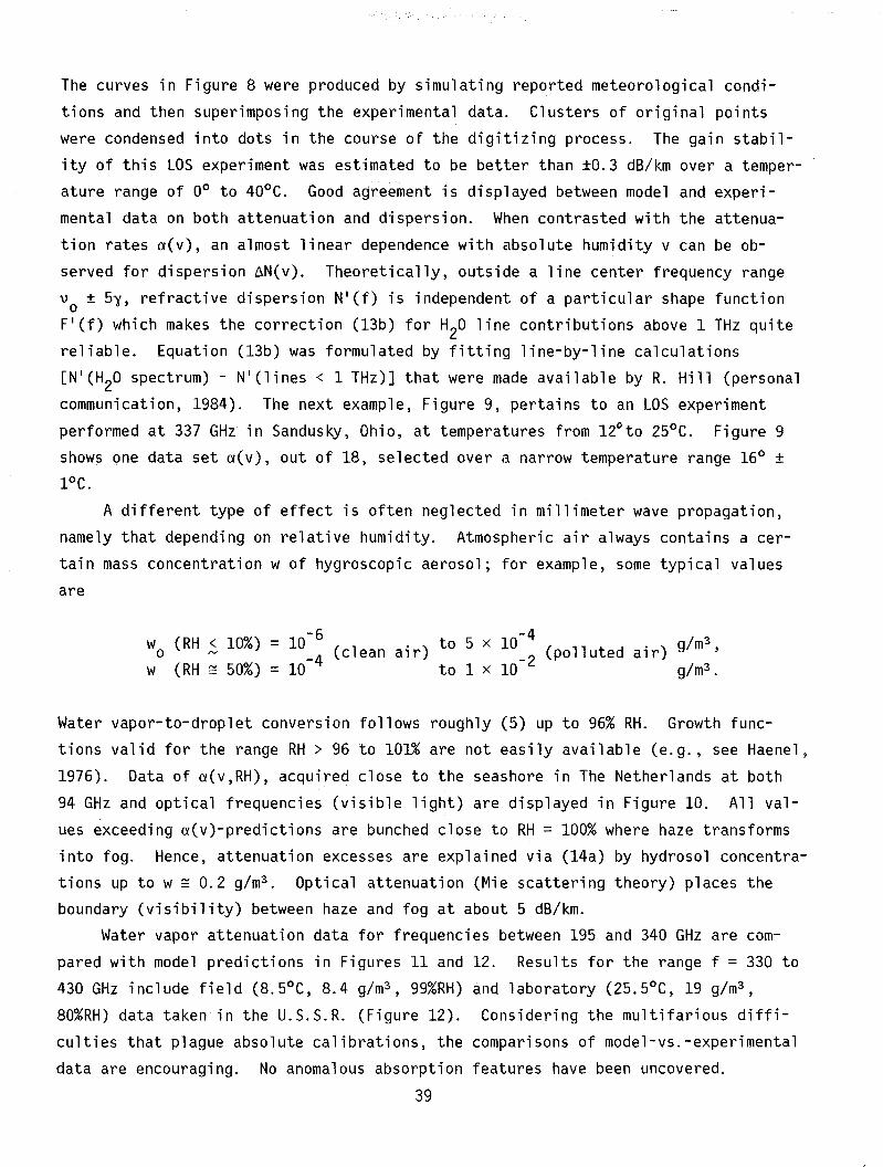
The curves in Figure 8 were produced by simulating reported meteorological condi­

tions and then superimposing the experimental data. Clusters of original points

were condensed into dots in the course of the digit.izing process. The gain stabil­

ity of this LOS experiment was estimated to be better than ±0.3 dB/km over a temper­

ature range of 0° t.o 40°C. Good agreement is displayed between model and experi­

mental data on bot.h attenuation and dispersion. When contrasted with the attenua­

tion rates a(v), an almost linear dependence with absolut.e humidity v can be ob­

served for dispersion ~N(v). Theoretically, outside a line center frequency range

V o ± 5y, refractive dispersion N'(f) is independent of a particular shape function

FI(f) which makes the correction (13b) for H20 line contributions above 1 THz quit.e

reliable. Equation (13b) was formulated by fitting line-by-line calculations

[N 1 (H20 spectrum) - N'(lines < 1 THz)] that were made available by R. Hill (personal

communication, 1984). The next example, Figure 9, pertains to an LOS experiment

performed at 337 GHz in Sandusky, Ohio, at temperatures from 12°to 25°C. Figure 9

shows one data set a(v), out of 18, selected over a narrow temperature range 16° ±

1°C.

A different type of effect is often neglected in millimeter wave propagation,

namely that depending on relative humidity. Atmospheric air always contains a cer­

tain mass concentration w of hygroscopic aerosol; for example, some typical values

are

wo (RH ~ 10%)w (RH ~ 50%)

= 10-6 to 5 x 10-4 g/m3(clean air) (polluted air) ,

= 10-4 to 1 x 10- 2 g/m3 •

Water vapor-to-droplet conversion follows roughly (5) up to 96% RH. Growth func­

tions valid for the range RH > 96 to 101% are not easily available (e.g., see Haenel,

1976). Data of a(v,RH), acquired close to the seashore in The Netherlands at both

94 GHz and optical frequencies (visible light) are displayed in Figure 10. All val­

ues exceeding a(v)-predict.ions are bunched close to RH = 100% where haze transforms

into fog. Hence, attenuation excesses are explained via (14a) by hydrosol concentra­

tions up to w =0.2 g/m3 • Optical attenuation (Mie scattering theory) places the

boundary (visibility) between haze and fog at about 5 dB/km.

Water vapor attenuation data for frequencies between 195 and 340 GHz are com­

pared with model predictions in Figures 11 and 12. Results for the range f = 330 to

430 GHz include field (8.5°C, 8.4 g/m3 , 99%RH) and laboratory (25.5°C, 19 g/m3 ,

80%RH) data taken in the U.S.S.R. (Figure 12). Considering the multifarious diffi­

culties that plague absolute calibrations, the comparisons of model-vs.-experimental

data are encouraging. No anomalous absorption features have been uncovered.

39

337 GHz

+

~ 10r­«:::>zwr- 5~

o L-....L.-.-.L.-.-..I--...L...-...L...-~...L..-...L-..&.-_~~__....I-.....

o 5 10 15ABSOLUTE HUMIDITY (g/m**3)

Sandusky LOS

d =0.50 kmh =0 kmP =101.3 kPa

Figure 9. Specific attenuation a for humid air at T = 16 ± 2°C and a frequencyof 337 GHz:

+ Measured data (Gasiewski, 1984)--- MPM, • RH = 100%

40

0.0 i-------------....,

1.0Ypenburg LOS

d =0.935 kmh = 0 kmP = 101. 3 kPaT =8 ± 8 °C

4 months of data(11/77-03/78)taken at the rate l/hr

7.0

10 vi s. light "

20--.... I.SE

.::L......... .

94 GHz 94 GHz0

co 0. 0-0 , o C.. \,-.....- 1.0 .- :~ .. 1.0.

" 0'(j ~

•0·· awz: •• #

0 -tt--l .S .5r- avc:::(=>z:wr- O.D 0.0r- 8.0 12.0 40 60 80 100c:::(

ABSOLUTE HUMIDITY v (91m3 ) RELATIVE HUMIDITY RH(%)

Figure 10. Attenuation rates a at 94 GHz and optical frequencies (visible light)as functions of absolute humidity v and relative humidity RH:

0, - Measured data (Buijs and Janssen, 1981)MPM

41

10

E P = 100.3 kPa~

v = 1. 0 g/m3"m'U.. (15% RH)Z

0I- 1<{:JZ

••+••• + ••w ••• ++ •• +

~••• •

W4

.1180 200 220 240 260

10

E~

" (b)m'U

.. T = -10°C (42% RH)Z0

~1

•:J •Z • • • • ++ • +w +. •

l-I-<(

W4

.1180 200 220 240 260

FREQUENCY, GHz

Figure 11. Water vapor attenuation rates a(v) across the atmospheric window rangeW4 at two temperatures, 5°and -10°C:

+ Measured data (Fedoseev and Koukin, 1984)MPM

42

1000

(a) FieldE

P = 96.9 kPa.:::l........m T = 8.5 °C"U

.. v = 8.4 91m3

Z0 100

99 %RH

~:JZW

~W6

10320 340 360 380 400 420

1000

(b)

E P = 97.3 kPaLaboratory

::t........m T = 25.5 °C"U

.. v = 19 91m3

Z 100 80 .3 % RH0

~:JZW

~ W6W5

10320 340 360 380 400 420

FREQUENCY, GHz

Figure 12. Water vapor attenuation rates a(v) across the atmospheric window rangesWS and W6 at two temperatures, 8.Soand 2S.5°C:

+ Measured data (Furashov et al., 1984)MPM

43

Analysis of raw data a(v,T) available from the experiments allows an estimate

of the negative temperature dependence eY. The exponent y was found to vary between

3.5 and 6 (Table 5), which is consistent with semiempirical theoretical results

( Li ebe, 1985).Path attenuation A = Ap + Av and atmospheric noise expressed by a brightness

temperature TB =Tp + Tv are closely related (e.g., Waters, 1976). Brightness temper­

atures T~ have been measured at six frequencies between 2.5 and 90 GHz in clear

weather with radiometers looking toward zenith from a mountain peak. At ho = 3.80 km,

a typical tropospheric water vapor content V (mm) is reduced to about one-fifth. In

fact, an average water vapor content was determined to be00

V =~ v(h)dh ~ 3 ± 1 mm.3.8 km

All experiments were conducted with utmost care for the purpose of measuring cosmicbackground radiation (2.8 K).

The MPM program was operated with a mean July climate for California that speci­

fied P(h), T(h), and v(h) profiles over the range h =3.8 to 30 km. Dry air zenith

attenuation Ap and a water vapor attenuation slope av ~ AviV were calculated by numer­

ical integration and listed in Table 7. Values of Ap have been converted into bright­

ness temperatures Tp by assuming an average temperature To = 260 K consistent with

the T(h) profile. Brightness data below 10 GHz are particularly sensitive to the

correct value of Yo in the dry air continuum (12a). Above 10 GHz, the water vaporslope av amounts to meaningful values. At 90 GHz, the data point (Tx - Tp)/33 =

1. 70 K/mm was used as a reference water vapor slope z to define an "equ ivalent"vtemperature of 305 K for conversions from path attenuation to medium brightness at

other frequencies. This way, all six T~-data in Table 7 are apportioned in a con­

sistent manner to dry and wet attenuation terms based upon MPM predictions.

In summary, good agreement between predicted and reported responses, foremostspecific attenuation, was found over a wide range of parameters--test frequencies

varied between 2.5 and 430 GHz and meteorological conditions as follows:

P = 70 to 101 kPa, T = -100 to 35°C, v = 0 to 25 g/m3 and RH = 0 to 99%. All in all,

some credibility can be given to the computer program MPM detailed in Section 2.1.

44

Table 7.

Summary of an MPM-Ana1ysis of Atmospheric Brightness T~ Measured at Frequencies

Between 2.5 and 90 GHz from a Mountain Peak (White Mountain, CA, ho = 3.80 km,

zenith path, clear weather, Po = 65 kPa, To = 6° ± 5°C)

Water Vapor Slope

(MPM)

Frequency Dry Air

(MPM)

f AdT a)p

GHz dB K

2.50 .0157 .9384.75 .0161 .9629.40 .0173 1. 034

10.0 .0175 1.04633.0 .0565 3.36190.0 .0909 5.385

dB/mm(V = 3.3 mm)

.00039

.00046

.00518

.0249

K/mm

0.0270.0320.362

1. 70

RADIOMETEREXPERIMENT

K(V ~ 3 mm)

.95(5)t

1.10(10)t1. 03(3)t1.15(10)*

4.51(18)*11. 00(20)*

= 10 10g[To/(To ~ Tp)] (dB)

= 260(1 - 10-0.lAp), where To = 260 K

References:

t Danese, L., Atmospheric emission:measurements of TCBR ' Istituto dicommunication, September 1984)

* Costales (1984)

models, comparison with data, consequences onAstronomia, Padova, Italy (personal

( ) Digits in parentheses give the deviation from the mean in terms of the final

listed digit.

45

4.4 Boulder LOS Results

The Colorado climate is not particularly well suited for studies of humidity

effects. Over the measurement period August 1983 to June 1984, absolute humidity

varied between v = 2 and 14 g/m3 , no fog events were recorded Cw ~ 0), and temper­

atures ranged between T = -8° and +36°C.

4.4.1 Water Vapor AttenuationsHumidity attenuation data for 97 days are shown in Figure 13 for 28.8 and

96.1 GHz. The 135 data points represent hourly means from nearly stationary condi­tions, usually afternoons. The data are organized into three temperature groups and

compared with MPM predictions. Generally, good agreement is found within the uncer­

tainties C± 0.05 dB/km) of the experiment. Only meteorological data CP, T, No) at

the receiver site have been used to determine via (30) the absolute humidity for

each point. The 28.8 GHz results represent relative values of a(v) obtained by a

IIbest ll fit to predictions.

Equ. (23)

2(f2/f1)

71

11

6.4

4.4.2 Turbulence Properties

Power spectral density W(w) and ratios W2/W1 are depicted in Figures 14 a

through c for the three events identified in Figure 5. Spectral density ratios are

independent of refractive structure parameter c~ and path length d. When the outer

scale of turbulence Qo > ~Ad, (Fresnel zone size), the variance as is expected to be

proportional to the 716 power of radio frequency f over a range of fluctuation fre­

quencies w according to (17). On the other hand, when Q «~, the variance al os

drops rapidly with w-8 3 and is proportional to the square of frequency f according

to (23). Hence, turbulence theory predicts for ratios W2/W1 different values in theturbulence regime (17) and the inertial subrange (23):

7/6f2/f1 (f2/f1)

96.1/11.4 12

96.1/28.8 4.1 Equ. (17)28.8/11.4 3.0

as marked in Figures 14 a-c. For the case where a strong, gusty wind provided a

well mixed atmosphere along the 27 km path, Figure 14b displays a reasonable fit

over a range of w between 0.01 and 0.2 Hz.

A two-parameter-fit CWo and wo) to the power spectral density Wwas attempted

with the following results:

46

Fi gure 13.

Water vapor attenua­tion at 28.8 and 96.1 GHz for atemperature range between -10° and40°C:

x, fj., • Measured data (14±22°C)MPM (see Figure 6)

• RH = 100%

Boulder LOSd = 27.2 kmh = 1. 65 kmp = 82 kPa

Curve ID Tur:-

I 02 103 204 305 40

·20

28.8 GHz

...........E .15~

"-ro"'0

........"

Z.10a

I-«::JZWI- .05~ ~ T

UCx 0±10fj. 20±5

30±5

.001.0

96.1 GHz

...........E~

"-ro"'0........"

Z.5a

~fA

::>zw

~

.0 L......i~---L---L---I-....L-...L.-.£...-..lL---L---L---L..-L-....L.-1

o 5 10 15

ABSOLUTE HUMIDITY (g/m 3 )

47

FIT j 6, 16. 16 pts,­

//

.p',V

7'.,('

----:-" 1

x X

10

"

X J«• <XX

~+x*+++

1 >1+

(b)

-

-~--x

..........3

(a)

------+---.±.--*- --x-

+ xx

102Curve 10:EXP. TH.

1+ 2x 3

10 -....3........

N3

t0.,....

++J tro • x x0:::

1 l-

X

1 .

1

m 256, 16 pts

.1.01

4 June 1984 1000-1700

.001

Hf •

10 ;'1;l'}f;

x x~

.1

.....

.01

28 Feb 1984 0900-1 600

VIc:QJ

Cl

.,....

Fluctuation Frequency w, Hz

U1

~ 4(2) ~Et gusty

Figure 14. Power spectral density W(w) and ratios W2/W1 for event time series shownin Figure 5:

a) see Figure Sab) see Figure Sb

48

(c)102 ..---r-..---r-~~-'-~~~--'-""""""-""""'"

(i)

10

x x +t

2 t_ - -,--

./

./,/ 1/

/"----"""'.

x_ - f _~-_- ~-X

----i t -""!. __'1.._ - - - - - 3+

+~

It

,,-4

~N

3= 10o.,....~ro~

+

-

m 256 ~t9

RANDOM GAUSSIAN DATA OF VARIANCE EQUAL TO 1

1 - .-+---Jf..,-·f-*-+*lI:llllllllllMllMllllIllIIIIIE IIIIIIIIl...

10-1..L--....-~~~--'--L- ...........~--''----'---'-'-'...........,J.001 .01 .1 11.1

FIT 256, 16 ~t9

.01

t • t

10 I-II)

CQ)

o

.,....

1 0 3lo-----.".-+--+-I--+-+-I-+++--I--+......-r_~--+--+-i-+-+-+++l

N

~ +~X\N Jl x+~+.!g 102 -. +" x + ' .

x +tt·.··.', 1x ++ --;::--""':":;,".-"

X 2 ~,::~~.,."":':~:,:,\

3~~~--~\~ ::,\;:}( ,x X\~~\ f+~' ~-\\;;

,....~ 1-~uQ)

0-

~ 10-1 -Q) , \

~ \o 19 May 1984 0600-0900 \~ \

10- 2L-~-,--,-.....................L--,--'--''-'-'-.......L----,----~'"''''''''''..001

Fluctuation Frequency w, Hz

UL ~ ±1 direction change, calm

Figure 14. continued:c). see Figure 5ci) Test of FFT

49

f .p:a- W w U1

W w U Wo Wo U10 0 0 0 l.

GHz m dB2/Hz Hz m/s dB2/Hz Hz m/s dB2/Hz Hz m/s

96.1 9.2 0.15 0.20 1.8 5.0 0.43 4.0 40 0.11 1.0

28.8 16.8 0.051 0.11 1.9 1.7 0.24 4.0 13 0.063 1.1

11.4 28.8 0.037 0.063 1.8 1.2 0.14 4.0 10 0.035 1.0Fiqure 14a 14b 14c

Respective asymptotes for Wand w-8/ 3 are shown in Figures 14 a-c. In each case,o

the deduced cross wind speed u is supported by actual measurements along the path.l.

On the whole, agreement between experiments and predictions is not too good; which

is to be expected, since the event periods are rather extended (i.e., 7 and 3 h) and

the path is 27 km long. The spectral density behavior W(f1) in Figure 14a is sus­

pected to have been influenced by an electronic problem unrelated to atmospheric

fluctuations. Automatic gain control of an LOS system will have to compensate at

least ± 20 dB (see suspected multipath event, Figure 14c). The spectral FFT ana­

lysis technique was tested with random data (Figure 14i).

5. CONCLUSIONS

Understanding the transmission effects through moist air on millimeter-wave

propagation has been the major topic of this report. Analytical and experimental

details have been given as they pertain to the formulation and validation of a physi­

cal model serving that purpose. A number of tests with realistic data tend to con­

firm, at least up to 430 GHz, that the program MPM converts routinely measured mete­

orological variables into attenuation and delay rates. Computation time is opti­

mized by addressing only the main absorbers H20 and O2, and by restricting line-by­

line calculations to spectral lines centered below 1000 GHz. In principle, about

150 strong (out of 3800) H20 lines between 1 and 15 THz can make additional contri­butions to millimeter-wave absorption and dispersion. The model utilizes 30 lines

and makes up for unaccounted terms with the empirical continuum (13). Further theo­

retical work into the physics of colliding H20-AIR molecules is needed in order to

find a plausible physical basis for the water vapor continuum and claim general val­idity for the MPM.

Performance predictions by analytical means are important for millimeter-wave

systems operating through the atmosphere since effort and risk in realizing new con­

cepts can be reduced to a large extent by simulating weather-related effects. Many

effects are folded into path-averaged signal levels at a receiver. By contrasting

clear-air data measured at multiple frequencies over several hours, factors such as

path attenuation and amplitude scintillations could be separated and applied to test

50

the appropriate models for moist air behavior. Results on turbulence-induced ampli­

tude scintillations support the assumption that generally these effects will not

seriously impair the performance of a system. More serious multipath effects were

suspected on a few occasions, although their occurrence was rare due to the rather

dry and well-mixed climate prevailing during the test period. Results in support of

a particular multipath model were not obtained.

ACKNOWLEDGMENT

Laboratory research work leading to the MPM program was supported in part by

the U.S. Army Research Office under Contract ARO 111-85.

51

6. REFERENCES

Allen, K. C., and H. J. Liebe (1983), Tropospheric absorption and dispersion ofmillimeter and submillimeter waves, IEEE Trans. Ant. Prop. AP-31, No.1, pp.221-223 [corrections AP-31, No.6, p. 1004]. -----

Allen, K. C., H. J. Liebe, and C. M. Rush (1983), Estimates of millimeter waveattenuation for 18 United States cities, NTIA Report 83-119 (available fromNTIS under Access. No. PB83-240630).

Bohlander, R. A., R. W. McMillan, and J. J. Gallagher (1985), Atmospheric effects onnear-millimeter-wave propagation, Proc. IEEE 73, No.1, pp. 49-60.

Boudouris, G. (1963), On the index of refraction of air, the absorption anddispersion of centimeter waves by gases, J. Res. NBS 670, No.6, pp. 631-684.

Buijs, J. H., and L. H. Janssen (1981), Comparison of simultaneous atmosphericattenuation measurements at visible light, infrared (3-5 ~m) and mm-waves (94GHz), Physics Lab., NORD, The Netherlands, Report No. PHL 1981-04, January.

Chang, A. T., and T. T. Wilheit (1979), Remote sensing of atmospheric water vapor,liquid water, and wind speed at the ocean surface by passive microwavetechniques from the NIMBUS 5 satellite, Radio Sci. 14, No.5, pp. 793-802.

Clifford, S. F., and J. W. Strohbehn (1970), The theory of microwave line-of-sightpropagation through a turbulent atmosphere, IEEE Trans. Ant. Prop. AP-18,No.2, pp. 264-274. -----

Cole, R. S., K. L. Ho, and N. O. Mavrokoukoulakis (1978), The effect of the outerscale of turbulence and wavelength on scintillation fading at millimeterwavelengths, IEEE Trans. Ant. Prop. AP-26, No.5, pp. 712-715.

Costales, J.B. (1984), Simultaneous measurements of atmospheric emission at 10, 33,and 90 GHz, Lawrence Berkeley Lab., Phys. Oiv., Report LBL-18744, November.

Crane, R. K. (1981), Fundamental limitations caused by RF propagation, Proc. IEEE69, No.2, pp. 196-209.

Oagg, I. R., L. A. Read, and J. Vanderkooy (1982), Far infrared laser system for themeasurement of collision-induced absorption spectra, Rev. Sci. Instr. 53,No.2, pp. 187-193. --

Espeland, R. H., E. J. Violette, and K. C. Allen (1984), Atmospheric channelperformance measurements at 10 to 100 GHz, NTIA Report 84-149, April (availablefrom NTIS under Access. No. PB84-211325).

Falcone, Jr., V. J., L. W. Abreu, and E. P. Shettle (1982), Atmospheric attenuationin the 30 to 300 GHz region using RAOTRAN and MWTRAN, SPIE 337 (Mm-WaveTechnology), pp. 62-66.

Fedoseev, L. I., and L. M. Koukin (1984), Comparison of the results of summer andwinter measurements of atmospheric water vapor absorption at wavelengths 1.5 to1.55 mm, Int'l. J. Infrared &Millimeter Waves ~, No.7, pp. 952-964.

52

Filho, F. M., D. A. Jayasuriya, R. S. Cole, and C. G. Helmis (1983), Spectral densityof millimeter wave amplitude scintillations in an absorption region, IEEETrans. Ant. Prop. AP-31, No.4, pp. 672-676.

Furashov, N. I., V. Y. Katkov, and V. Y. Ryadov (1984), On the anomalies ofsubmillimeter absorption spectrum of atmospheric water vapor, Int'l. J.Infrared &Millimeter Waves ~, No.7; pp. 971-981.

Gasiewski, A. J. (1983), Atmospheric propagation loss measurements in the spectralwindow at 337 gigahertz, Technical Report No. MMW 2-83, August (EE &AP Dept.,Case Western University).

Haenel, G. (1976), The properties of atmospheric aerosol particles as functions ofthe relative humidity ... , Advances in Geophys. 19, pp. 77-188 (Academic Press,NY). --

Harris, F. J. (1978), On the use of windows for harmonic analysis with the discreteFourier transform, Proc. IEEE 66, No. I, pp. 51-83.

Hill, R. J., and S. F. Clifford (1981), Contribution of water vapor resonances tofluctuations of refraction and absorption for sub mm through cm wavelengths,Radio Sci. 16, No. I, pp. 77-82.

Hill, R. J., R. S. Lawrence, and J. T. Priestley (1982), Theoretical andcalculational aspects of the radio refractive index of water vapor, Radio Sci.17, No.5, pp. 1251-1257.

Ishimaru, A. (1972), Temporal frequency spectra of multifrequency waves in turbulentatmosphere, IEEE Trans. Ant. Prop. AP-20, No. I, pp. 10-19.

Liebe, H. J., and J. Hopponen (1977), Variability of EHF air refractivity withrespect to temperature, pressure, and frequency, IEEE Trans. Ant. Prop.AP-25, No.3, pp. 336-345.

Liebe, H. J. (1981), Modeling attenuation and phase of radio waves in air atfrequencies below 1000 GHz, Radio Sci. 16, No.6, pp. 1183-1199.

Liebe, H. J. (1983), An atmospheric millimeter wave propagation model, NTIA Report83-137, December (available from NTIS under Access. No. PB84-14394).

Liebe, H. J. (1984), The atmospheric water vapor continuum below 300 GHz, Int'l J.Infrared &Millimeter Waves ~, No.2, pp. 207-227.

Liebe, H. J. (1985), An updated model for millimeter wave propagation in moist air,Radio Sci. 20 (in press).

Manabe, T., Y. Furuhama, T. Ihara, S. Saito, H. Tanaka, and A. Ono (1984),Measurements of attenuation and refractive dispersion due to atmospheric watervapor at 80 and 240 GHz, Conf. Digest, 9th Intll. Conf. on Infrared &Millimeter Waves, Takarazuka, Japan F-3-3, pp. 465-466.

Oppenheim, A. V. and R. W. Schafer (1975), Digital Signal Processing (Prentice-Hall,Inc.).

53

Orlanski, I. (1975), A rational subdivision of scales for atmospheric processes,Bulletin A.M.S. 56, No.5, pp. 527-530.

Ott, R. T. and M. C. Thompson, Jr. (1978), Atmospheric amplitude spectra in anabsorption region, IEEE Trans. Ant. Prop. AP-26, No.2, pp. 329-332.

Rosenkranz, P. W. (1975), Shape of the 5 mm oxygen band in the atmosphere, IEEETrans. Ant. Prop. AP-23, No.4, pp. 498-506.

Rosenkranz, P. W. (1982), Comment on absorption and dispersion in the O2 microwavespectrum at atmospheric pressures, J. Chern, Phys. 77, No.4, pp. 2216-2216.

Rummler, W. D. (1979), A new selective fading model; application to propagationdata, Bell Sys. Tech. J. 58, No.5, pp. 1037-1071.

Simpson, O. A., B. L. Bean, and S. Perkowitz (1979), Far infrared optical constantsof liquid water measured with an optically pumped laser, J. Opt. Soc. Am.Lett. 69, No. 12, pp. 1723-1726.

Stankevich, K. S. (1974), Absorption of sub-millimeter-range radio waves in a dryatmosphere (Engl. Transl.), Radiophys. Quantum Electron. 17, pp. 579-581.

Stephansen, E. T. (1981), Clear-air propagation on line-of-sight radio path: areview, Radio Sci. 16, No.5, pp. 609-629.

Tatarski, V. I. (1961), Wave Propagation in a Turbulent Medium, translated fromRussian by R. A. Silverman (McGraw-Hill, New York).

Violette, E. J., R. H. Espeland, and K. C. Allen (1983), A diagnostic probe toinvestigate propagation at millimeter wavelengths, NTIA Report 83-128, August(NTIS Access. No. PB84-104223).

Vogel, W. J., J. H. Davis, and C. E. Mayer (1984), Line-of-sight observations at 86GHz with a very large and a small antenna, IEEE Trans. Ant. Prop. AP-32, No.2,pp. 113-118. -----

Waters, J. R. (1976), Absorption and emission by atmospheric gases, in Methods ofExperimental Physics, 12B, edited by M. L. Meeks, Chapter 2.3 (Academic Press,New York).

54

FORM NTIA-29 U.S. DEPARTMENT OF COMMERCE(4-80) NAT'L. TELECOMMUNICATIONS AND INFORMATION ADMINISTRATION

BIBLIOGRAPHIC DATA SHEET

1. PUBLICATION NO. 2. Gov't Accession No. 3. Recipient's Accession No.

NTIA Report 85-171

4. TITLE AND SUBTITLE 5. Publication Date

r~i 11 imeter-Wave Propagation in Moist Air: Model versus r,1arch 1985Path Data 6. Performing Organization Code

NTIA/ ITS. S37. AUTHOR~E Tl Project/Task/Work Unit No.H.J.LIE ,K.C.ALLEN,G.R.HAND,R.H.ESPELAND, AND E.J.VIOLE8. PERFORMING ORGANIZATION NAME AND ADDRESS 91 081 08U.S. Dept of Commerce/Nat'l Telecommunications &

Information Administration/Institute for Telecommuni- 10. Contract/Grant No.

cation Sciences/S3325 BroadwayOn "rl,.,,,, rn Qn':ln':l11. ~ponsori~g Cflanization Name and Addrry 1 ..

&12. Type of Report and Period Covered

U.S. Dept 0 Commerce/ Nat Te ecommunlcatlonsInformation Administration

Herbert C. Hoover Building 13.

WnRiRaf8R~tbcut~~~38venue, N.W.14. SUPPLEMENTARY NOTES

15. ABSTRACT (A 200-word or less faclual summary of most significant information. If document includes a significant bibliography or literature

A p}ac~ft~fng£mo~pheric millimeter-wave propagation model (MPM) is updated andtested with experimental data from hori zonta1, 1 i ne-of-s i ght lir.ks when there is noprecipitation. The MPM computer program predicts attenuation and delay propertiesof moist air over ranges in frequency from 1 to 1000 GHz and in height from o to30 km. Input variables are radio path distributions of pressure, temperature,relative humi di ty, and a suspended droplet concentration simulating haze and fogconditions. Terrestrial path data from millimeter-wave propagation experiments,including those from a 27 km link operated at 11.4, 28.3, and 96.1 GHz by theInstitute for Telecommunication Sciences (ITS) , have been analyzed. Calibratedmean signal levels permitted studies of water vapor losses. In addition, a spectralanalysis was performed of clear-air scintillations caused by turbulence. Ingenera1 , good agreement is obtained with the ~PM for test frequencies up to 430 GHz.

16. Key Words (Alphabetical order, separated by semicolons)

atmospheric attenuation and delay; millimeter wave properties of moist air;propagation program MPM; terrestrial radio path data

17. AVAILABILITY STATEMENT 18. Security Class. (This report) 20. Number of pages

>[] UNLIMITED. UNCLASS I FI ED 62

19. Security Class. (This page) 21. Price:

D FOR OFFICIAL DISTRIBUTION.

UNCLASSI FI ED

li- u.s. GOVERNMENT PRINTING OFFICE:1985-576-000 I 20017