EI~,EVIER Physica D 103(1997)537-553

PHYSlCA ®

Migration in cellular automata

Birgitt Sch6nfisch a,*, Claude Lacoursi~re b

a Universitiit Tiibingen, Lehrstuhlfiir Biomathematik, Aufder Morgenstelle I0. 72076 Tiibingen. Germany b Physics Department and Center for Nonlinear Dynamics in Physiology and Medicine, McGill University,

3655 Drummond. Montreal, Que., H3G I Y6 Canada

Abstract

We investigate the effect of spatial migration of cells in cellular automata that have been used in the study of excitable media and epidemiology, with an infinite range migration. While the periods of oscillation of the densities of cells in each state are mostly unaffected by migration, the amplitudes of these oscillations behave very differently when migration is present. Spatial structures which develop in the absence of migration are shown to be unstable to even the lowest possible level of migration. Decay of these structures is shown to scale with system size, demonstrating the absence of structure in the asymptotic regime fi~r any system size. Decay of structure is also shown to occur on a time scale, T, scaling roughly as T ~ t • m, where m is the migration rate and t is time elapsed. The exact shape of the decay of structure, however, is not self-similar, Overall, structure decays almost entirely after each cell has migrated twice on an average. We conclude from this that the asymptotic behavior, after the structure has subsided, is governed by the mean field approximation.

1. Introduct ion

It is well known that even the simplest cellular automata are capable of complex behavior in time and space as

seen in [ 14]. There is great interest in their relationship with analytical models such as ordinary or partial differential

equations. Some advances have been made in this direction in the field of fluid mechanics, for instance [15]. One

can compare computing efficiency of cellular automata versus ordinary differential equations, or partial differential

equations, as well as modeling efficiency. A recent example of this is the paper by DeRoos et al. [7] in which

they compared cellular automata and ordinary differential equations predator-prey models. Similarly, Boccara and

Cheong [4] and Boccara et al. [5] compared cellular automata and ordinary differential equations epidemic models.

They showed that with the introduction of a mixing procedure, i.e., a set of extra rules that exchange the elementary

states of the cells, cellular automata become well approximated by difference equations obtained from the mean field

approximation. Boccara et al. [6] also introduced migration in predator-prey cellular automata models, where they

observed that the densities of cells in certain states approximate the values expected from the mean field theory, as the strength of the long range migration increased. This suggests that the accuracy of the mean field approximation

depends on the ability of the system to create and maintain spatial patterns.

* Corresponding author.

0167-2789/97/$17.00 Copyright © 1997 Elsevier Science B.V. All rights reserved t ' 1 1 S 0 1 6 7 - 2 7 8 9 ( 9 6 ) 0 0 2 8 4 - 9

538 B. Sch6nfisch, C. LacoursiOre / Physica D 103 (1997) 537 553

A mixing procedure can prevent structure from emerging, or force all structure to decay eventually. However, not all mixing procedures destroy all possible structures. For instance, mixing procedures of diffusive type, i.e.,

those with finite range, can in some cases allow the appearance of stable spatial patterns, like in reaction~liffusion systems.

In what follows, we present a specific example of mixing which destroys all structure in a class of cellular

automata. We do this by demonstrating that the decay of a scalar structure quantifier, which is zero for a lattice of

random O's and l 's, satisfies an approximate scaling relation in the effective migration rate fit and the system size

- G - and the time t, namely, ~(t, fit, IGI) ~ t • f i t / I G I , for late time. Using this scaling relation, and the fact that

systems with a specific system size and migration rate decay towards zero structure, we conclude that systems of any

size and any non-zero migration rate decay towards zero structure eventually. We also investigate the differences of

the dynamics of these cellular automata in the presence and absence of infinite range migration.

The paper is structured as follows: Section 1 presents the definitions of the cellular automata and the type of

migration we investigate; Section 2 presents the differences in the dynamics of migrating cellular automata versus

non-migrating ones, concentrating on the behavior of the density of infectious cells; Section 3 presents the differences

in the spatial structure between migrating and non-migrating automata; Section 4 presents results on the scaling

relation in the evolution of the structure of the migrating automata; and Section 5 summarizes the results.

1.1. C e l l u l a r a u t o m a t a

We consider a class of cellular automata which are simple models for epidemics. These are known as Greenberg-

Hastings automata [9,10] in the context of excitable media. For notation, we follow [12]. A cellular automaton,

A = (G, U, E, f0), is defined by a grid G of cells, a neighborhood U, a finite set of elementary states E, which

are the states of the cells, and a local function f0 that defines the dynamics. In particular, we consider the two- dimensional square grid G C 77 2. In simulations the grid is always finite, and to achieve translation invariance

the grid is closed to a torus. We choose the Moore neighborhood U = {x: Ixj[ < 1 }, where x is the coordinate

vector of the cell at the grid point x, and x j , j = 1 . . . . . d , are the Cartesian coordinates of x and d is the

dimension of the grid. For convenience, we let the grid G have the Euclidean norm. The set of elementary states

are natural numbers E = {0, rl . . . . . rg, i l . . . . . ia}, where 0 is interpreted as a susceptible or resting state, states

between ia and il are interpreted as infectious (and contagious), and the states between rl and rg are interpreted as

immune (non-susceptible and non-contagious). These elementary states model several infectious or excited stages,

as well as several immune stages, which are visited in sequence after an infection (or excitation, depending on the

interpretation). This means that if a cell has value k at time t, k > 1, then, the value of the cell is k - 1, at time t + 1,

without regard to the state of the neighborhood. Let z be a state (of the grid) and U (x) the neighborhood of a cell x.

Using the translation invariance of G we define the local function by the local function acting on the neighborhood of zero

a + g

f o ( z [ u ( o ) ) = 0

z(O) - I

f o r z ( 0 ) = 0 and s > g , f o r z ( 0 ) = 0 and s < g , otherwise

with s ----- s ( z l u ( o ) ) = #{x c U(0 ) :g < z ( x ) < a + g} is the number of infectious or excited cells in the neighborhood. A cell is infected if at least g neighbors are infectious.

Note that in what follows, we specialize to g = 0, i.e., we do not include immune stages, and we set g = 1, i.e.,

a single infectious neighbor is sufficient to make a cell infectious. We also perform synchronous updates of all the cells.

B. SchOnfisch. C. Lacoursibre/Physica D 103 (1997) 537-553 539

1.2. Migration

With the introduction of a stochastic migration procedure, we leave the field of classical cellular automata. After

applying the local function synchronously to all the cells, a migration rule is applied m times sequentially, which

exchanges the elementary states of some sites on the grid.

Elementary states cannot be moved individually since there are no 'empty ' cells on the grid. We consider a rule

where the elementary states of two cells chosen at random, uniformly on the whole grid, are exchanged. This is

an infinite range migration rule which should provide for good mixing. More realistic migration rules, from the

biological point of view, would exchange the elementary states of sites that are r units apart, with a rate that depends

on r. If the rate p at which two cells are exchanged decays to 0 as the distance between them increases, the rule is

said to have finite range. Otherwise, the rule has infinite range. More precisely, let the distance between two cells

be r. Then, if the rate of exchange behaves as p ~ exp ( - r / F ) , as r --+ ~ , the rule has finite range F. Otherwise,

if p ~ r -~ as r ~ w , the rule is said to have long range if ~ > 0 and infinite range for c~ _< 0. Our.interest

here is limited to the study of systems that are globally mixed. Seen from the viewpoint of dynamical systems,

the state space of automata with migration is the same as that of classical cellular automata, but the transitions are

more complex. Each state now has many non-zero transition rates to different states. Another viewpoint would be

to include the migration sequence in the state of the automaton, making the state space much larger. These automata

can then be interpreted as non-autonomous cellular automata.

Automata with migration can be compared to a partial differential equation using the framework that follows. Let

p(z(x) , t) be the probability that the cell at site x has value z at time t. Let D ( x , y ) be the kernel of the stochastic

migration operator, i.e., the probability that the cell at site x moves to sitey. Then, it is straightforward to show that

the following equation holds:

n

p(z (xo ) , t + 1)----- ~ Z I--I{D(yi'xi)p(zi(Yi)'t)}~A)(:o(xo),U<xo)),z(xo )" (1) yO,.. . ,ynEG ZO ..... Zn~E i

The symbol 6,, m n, m E Y,is the Kronecker delta function

1 i fn = m,

~J~,,n = 0 otherwise.

The migration rule under consideration is as follows:

1 - D 0 i f x = y , 19(x, y) = 79o otherwise,

and it satisfies the sum rule: ~ y D ( X , y) = 1. A partial differential equation can be obtained from Eq. ( 1 ), taking the

limit of infinite system size and changing the sums into integrals. We find that because our kernel does not decay to

zero as Ix - Yl ~ cx~, we cannot recover a reaction~liffusion out of our system.

1.2.1. Effective migration rate Our migration procedure is to pick two cells, at positions x j, x2, uniformly on the grid G, and exchange their

values. This rule is applied m times sequentially. At the end of the procedure, some of the 2m cells that were picked and moved, will have regained their original elementary states. This happens because there is a non-zero probability to pick, for instance, the pair (xl, Xl ), which effects no migration. This suggests that the number m is biased measure

of the real migration rate. We must therefore consider the 'effective migration rate', which is an unbiased measure

of the amount of mixing that takes place when the procedure described above is applied m times.

540 B. Sch6nfisch, C. Lacoursibre / Physica D 103 (1997) 537-553

0.8

0.6

>o .=

0.4

0.2

I I I I I I I

0.5 1.0 1.5 2.0 2.5 3.0 3.5 4.0 ~ 1

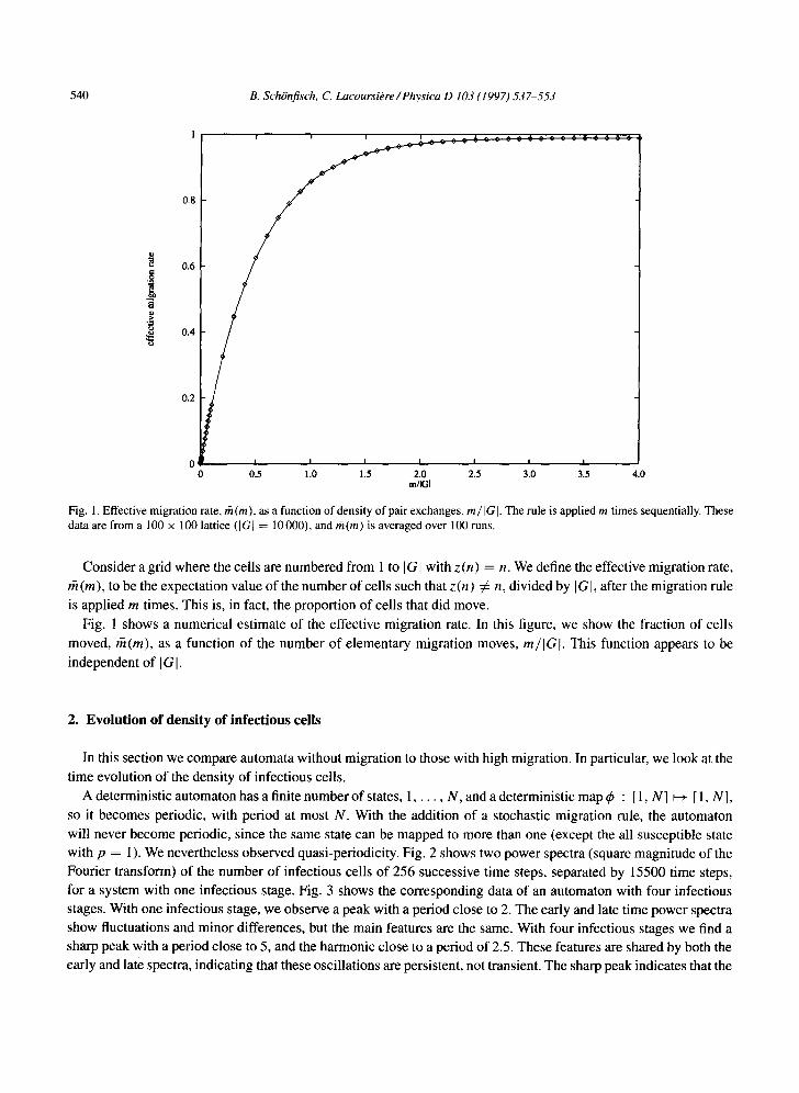
Fig. 1. Effective migration rate, fit (m), as a function of density of pair exchanges, rn/Ia]. The rule is applied m times sequentially. These data are from a 100 × 100 lattice ([G] = 10000), and fit(m) is averaged over 100 runs.

Consider a grid where the cells are numbered from 1 to [al with z (n ) = n. We define the effective migration rate,

rh (m), to be the expectation value of the number of cells such that z (n) ¢ n, divided by I GI, after the migration rule is applied m times. This is, in fact, the proportion of cells that did move.

Fig. 1 shows a numerical estimate of the effective migration rate. In this figure, we show the fraction of cells

moved, rh(m), as a function of the number of elementary migration moves, m / I G I . This function appears to be

independent of I GI.

2. Evolution of density of infectious cells

In this section we compare automata without migration to those with high migration. In particular, we look at the

time evolution of the density of infectious cells.

A deterministic automaton has a finite number of states, 1 . . . . . N, and a deterministic map <p : [ 1, N] ~-~ [ 1, N],

so it becomes periodic, with period at most N. With the addition of a stochastic migration rule, the automaton

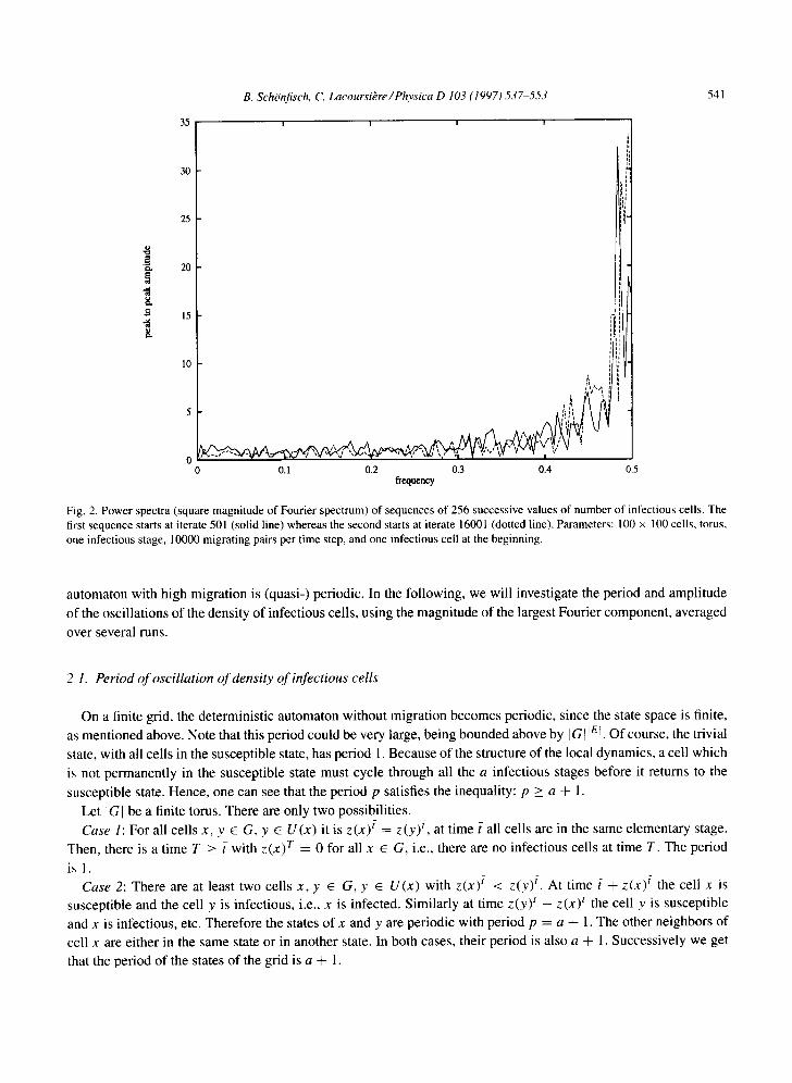
will never become periodic, since the same state can be mapped to more than one (except the all susceptible state with p = 1). We nevertheless observed quasi-periodicity. Fig. 2 shows two power spectra (square magnitude of the

Fourier transform) of the number of infectious cells of 256 successive time steps, separated by 15500 time steps,

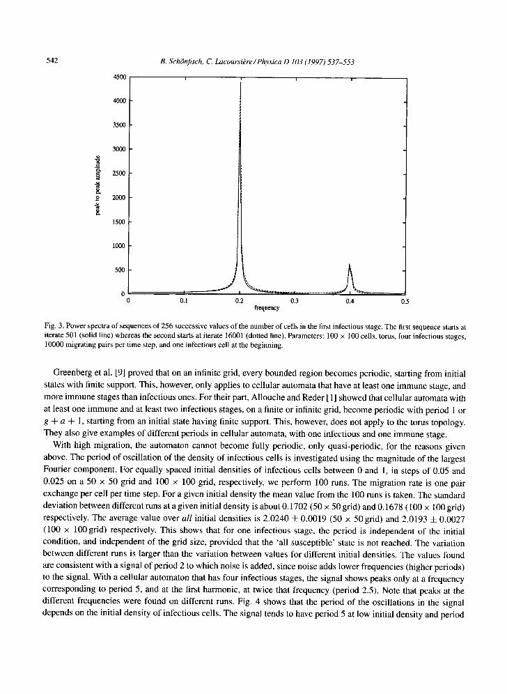
for a system with one infectious stage. Fig. 3 shows the corresponding data of an automaton with four infectious stages. With one infectious stage, we observe a peak with a period close to 2. The early and late time power spectra show fluctuations and minor differences, but the main features are the same. With four infectious stages we find a

sharp peak with a period close to 5, and the harmonic close to a period of 2.5. These features are shared by both the early and late spectra, indicating that these oscillations are persistent, not transient. The sharp peak indicates that the

35

30

25

20

15

I0

B. Sch6nfisch, C. Lacoursikre / Physica D 103 (1997) 537-553

I ! I l

0.1 0.2 0.3 0.4 0.5 frequency

541

Fig. 2. Power spectra (square magnitude of Fourier spectrum) of sequences of 256 successive values of number of infectious cells. The first sequence starts at iterate 501 (solid line) whereas the second starts at iterate 16001 (dotted line). Parameters: 100 × 100 cells, torus, one infectious stage, 10000 migrating pairs per time step, and one infectious cell at the beginning.

automaton with high migration is (quasi-) periodic. In the following, we will investigate the period and amplitude

of the oscillations of the density of infectious cells, using the magnitude of the largest Fourier component, averaged

over several runs.

2 1. Period o f oscillation o f density o f infectious cells

On a finite grid, the deterministic automaton without migration becomes periodic, since the state space is finite,

as mentioned above. Note that this period could be very large, being bounded above by I GI I El. Of course, the trivial

state, with all cells in the susceptible state, has period 1. Because of the structure of the local dynamics, a cell which

is not permanently in the susceptible state must cycle through all the a infectious stages before it returns to the

susceptible state. Hence, one can see that the period p satisfies the inequality: p >_ a + 1.

Let IGI be a finite torus. There are only two possibilities.

Case 1: For all cells x, y ~ G, y E U(x ) it is z(x) i = z (y) i, at time i a l l cells are in the same elementary stage.

Then, there is a time T _> { with z (x ) r = 0 for all x e G, i.e., there are no infectious cells at time T. The period

i.~ 1. Case 2: There are at least two cells x, y E G, y ~ U(x ) with z (x ) i < z(y) ?. At time ? + z(x) ? the cell x is

susceptible and the cell y is infectious, i.e., x is infected. Similarly at time z(y) i - z (x) ~ the cell y is susceptible

and x is infectious, etc. Therefore the states of x and y are periodic with period p = a + I. The other neighbors of

cell x are either in the same state or in another state. In both cases, their period is also a + I. Successively we get

that the period of the states of the grid is a + I.

542

4500

B. Schrnfisch, C. Lacoursikre /Physica D 103 (1997) 537-553

i I i

"v-,

o

8.

4000

3500

3000

2500

2000

1500

1000

500

0 , ...................... __A._..... 0.l 0.2 0.3 0.4 0.5

frequency

Fig. 3. Power spectra of sequences of 256 successive values of the number of cells in the first infectious stage. The first sequence starts at iterate 501 (solid line) whereas the second starts at iterate 16001 (dotted line). Parameters: 100 × 100 cells, torus, four infectious stages, 10000 migrating pairs per time step, and one infectious cell at the beginning.

Greenberg et al. [9] proved that on an infinite grid, every bounded region becomes periodic, starting from initial

states with finite support. This, however, only applies to cellular automata that have at least one immune stage, and

more immune stages than infectious ones. For their part, Allouche and Reder [ 1 ] showed that cellular automata with at least one immune and at least two infectious stages, on a finite or infinite grid, become periodic with period 1 or

g + a ÷ 1, starting from an initial state having finite support. This, however, does not apply to the torus topology. They also give examples of different periods in cellular automata, with one infectious and one immune stage.

With high migration, the automaton cannot become fully periodic, only quasi-periodic, for the reasons given

above. The period of oscillation of the density of infectious cells is investigated using the magnitude of the largest Fourier component. For equally spaced initial densities of infectious cells between 0 and 1, in steps of 0.05 and

0.025 on a 50 x 50 grid and 100 x 100 grid, respectively, we perform 100 runs. The migration rate is one pair

exchange per cell per time step. For a given initial density the mean value from the 100 runs is taken. The standard deviation between different runs at a given initial density is about 0.1702 (50 × 50 grid) and 0.1678 (100 x 100 grid)

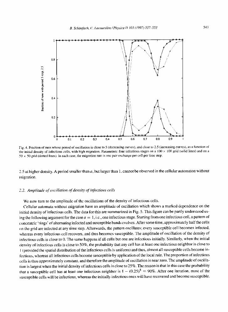
respectively. The average value over all initial densities is 2.0240 4- 0.0019 (50 × 50grid) and 2.0193 4- 0.0027 (100 x 100 grid) respectively. This shows that for one infectious stage, the period is independent of the initial condition, and independent of the grid size, provided that the 'all susceptible' state is not reached. The variation between different runs is larger than the variation between values for different initial densities. The values found are consistent with a signal of period 2 to which noise is added, since noise adds lower frequencies (higher periods) to the signal. With a cellular automaton that has four infectious stages, the signal shows peaks only at a frequency corresponding to period 5, and at the first harmonic, at twice that frequency (period 2.5). Note that peaks at the different frequencies were found on different runs. Fig. 4 shows that the period of the oscillations in the signal depends on the initial density of infectious cells. The signal tends to have period 5 at low initial density and period

B. SchOnfisch, C. Lacoursi~re / Physica D 103 (1997) 537-553 543

u ~

e,i

8.

.4

0.8

0.6

0.4

0.2

0 0.1 0.2 0.3 0.4 0.5 0.6 0.7 0.8 0.9

Fig. 4. Fraction of runs whose period of oscillation is close to 5 (decreasing curves), and close to 2.5 (increasing curves), as a function of the initial density of infectious cells, with high migration. Parameters: four infectious stages on a 100 × 100 grid (solid lines) and on a 50 × 50 grid (dotted lines). In each case, the migration rate is one pair exchange per cell per time step.

2.5 at higher density. A period smaller than a, but larger than 1, cannot be observed in the cellular automaton without

migration.

2.2. Amplitude of oscillation of density of infectious cells

We now turn to the amplitude of the oscillations of the density of infectious cells.

Cellular automata without migration have an amplitude of oscillation which shows a marked dependence on the

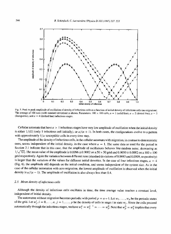
initial density of infectious cells. The data for this are summarized in Fig. 5. This figure can be partly understood us-

ing the following argument for the case a = 1, i.e., one infectious stage. Starting from one infectious cell, a pattern of

concentric 'rings' of alternating infected and susceptible bands evolves. After some time, approximately half the cells

on the grid are infected at any time step. Afterwards, the pattern oscillates; every susceptible cell becomes infected,

whereas every infectious cell recovers, and thus becomes susceptible. The amplitude of oscillation of the density of

infectious cells is close to 0. The same happens if all cells but one are infectious initially. Similarly, when the initial

density of infectious cells is close to 50%, the probability that any cell has at least one infectious neighbor is close to

I (provided the spatial distribution of the infectious cells is uniform) and thus, almost all susceptible cells become in-

fectious, whereas all infectious cells become susceptible by application of the local rule. The proportion of infectious cells is thus approximately constant, and therefore the amplitude of oscillation is near zero. The amplitude of oscilla-

tion is largest when the initial density of infectious cells is close to 25%. The reason is that in this case the probability that a susceptible cell has at least one infectious neighbor is 1 - (0.25) 8 ~ 90%. After one iteration, most of the

susceptible cells will be infectious, whereas the initially infectious ones will have recovered and become susceptible.

544 B. Sch~nfisch, C. Lacoursikre /Physica D 103 (1997) 537-553

0.7

o. - . . 0.6 ~ : ~ . ~ ' ~ . : , : .

0.5 ~ ,~ , . "m,:.,

/ / ,, , .: ,, ,, . '~ ~1. x

0.4

• ,, '1, " ~ l ~,, 0.3 '"I m'.ll I

: i . te : ; : ",

0.2 i ",

0 ~ I I I

0 0.1 0.2 0.3

0.1

¢' /

I / i l l "

• . p x • / • ~ x

0.4 0.5 0.6 0.7 0.8 0.9 1.0 initial density of infectious

Fig. 5. Peak to peak amplitude of oscillation of density of infectious cells as a function of initial density of infectious cells (no migration). The average of 100 runs (with standard deviation) is shown. Parameters: 100 x 100 cells, a = 1 (solid line), a = 2 (dotted line), a = 3 (linespoints), and a = 4 (dashed line) infectious stages.

Cellular automata that have a > 1 infectious stages have very low ampli tude of oscil lat ion when the initial density

is either 1/IGI (only 1 infectious cell initially), or a/(a ÷ 1). In both cases, the configurat ions evolve to a pattern

with approximately 1/a susceptible cells in every t ime step.

The ampli tude of the density of infectious cells, in the cellular automata with migrat ion, in contrast to determinist ic

ones, seems independent of the initial density, in the case where a = 1. The same data as used for the period in

Section 2.1 indicate that in this case, that the ampli tude of oscil lations behaves like random noise, decreasing as

1 / I ~ - / . The mean value of the ampli tude is 0 .0096 ± 0.0002 on a 50 x 50 grid and 0.0050 + 0.0002 on a 100 × 100

grid respectively. Again the variation be tween different runs (standard deviat ions of 0.0693 and 0.0509, respectively)

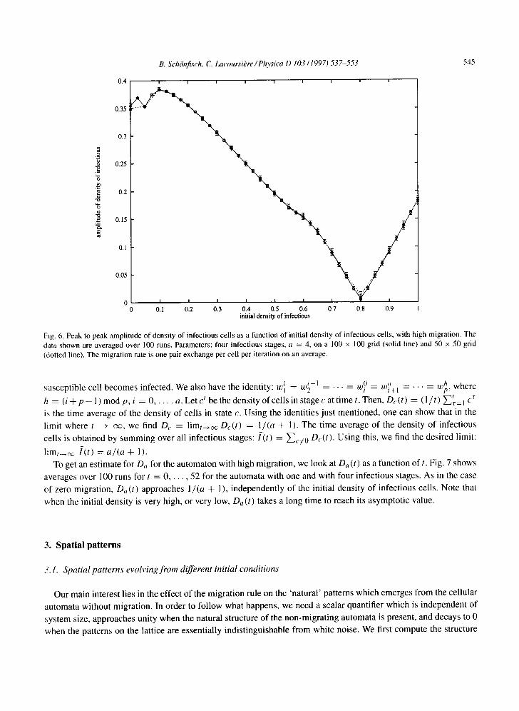
is larger than the variation of the values for different initial densities. In the case of four infectious stages, a = 4

(Fig. 6), the ampli tude still depends on the initial condit ion, and seems independent of the system size. As in the

case of the cel lular automaton with zero migrat ion, the lowest ampli tude of oscil lat ion is observed when the initial

densi ty is a/(a ÷ 1). The ampli tude of osci l lat ion is also always less than 0.4.

2.3. Mean density of infectious cells

Although the density of infectious cells oscillates in time, the t ime average value reaches a constant level, independent o f initial density.

The automaton without migrat ion becomes periodic with period p = a + 1. Let w] . . . . . Wp be the periodic states

of the grid. Let wj , i = 0 . . . . . a , j ---- 1 . . . . . p be the density of cells in stage i in state wj. Since the cells proceed

, - l _ • = wp °. Note that w ° ~ implies that every automatical ly through the infectious stages, we have w~ = w 2 -- - • ---- w

0.4

B. SchOnfisch, C. Lacoursibre/Physica D 103 (1997) 537-553

I I I ! I t I I

545

0.35 i

0.3

...q 0,25

0.2

0.15

0. I

0.05

I I I I I I I I ' I I

0.1 0.2 0,3 0.4 0.5 0.6 0,7 0.8 0.9 l initial density of infectious

Fig. 6. Peak to peak amplitude of density of infectious cells as a function of initial density of infectious cells, with high migration. The data shown are averaged over 100 runs. Parameters: four infectious stages, a = 4, on a 100 x 100 grid (solid line) and 50 x 50 grid (dotted line). The migration rate is one pair exchange per cell per iteration on an average.

i i - I Ot a h where susceptible cell becomes infected. We also have the identity: w I = w 2 . . . . . w = wi+ l . . . . . Wp, ~-- • - ~ Z r = l c'r h = ( i + p - l ) m o d p , i 0, . ,a . Letctbethedensityofcellsinstagecatt imet. Then, Dc(t) ( l / t )

is the time average of the density of cells in state c. Using the identities just mentioned, one can show that in the

limit where t --~ ~ , we find Dc = l i m t ~ De(t) = l / (a + l). The time average of the density of infectious

cells is obtained by summing over all infectious stages: [(t) = ~e~o De(t). Using this, we find the desired limit:

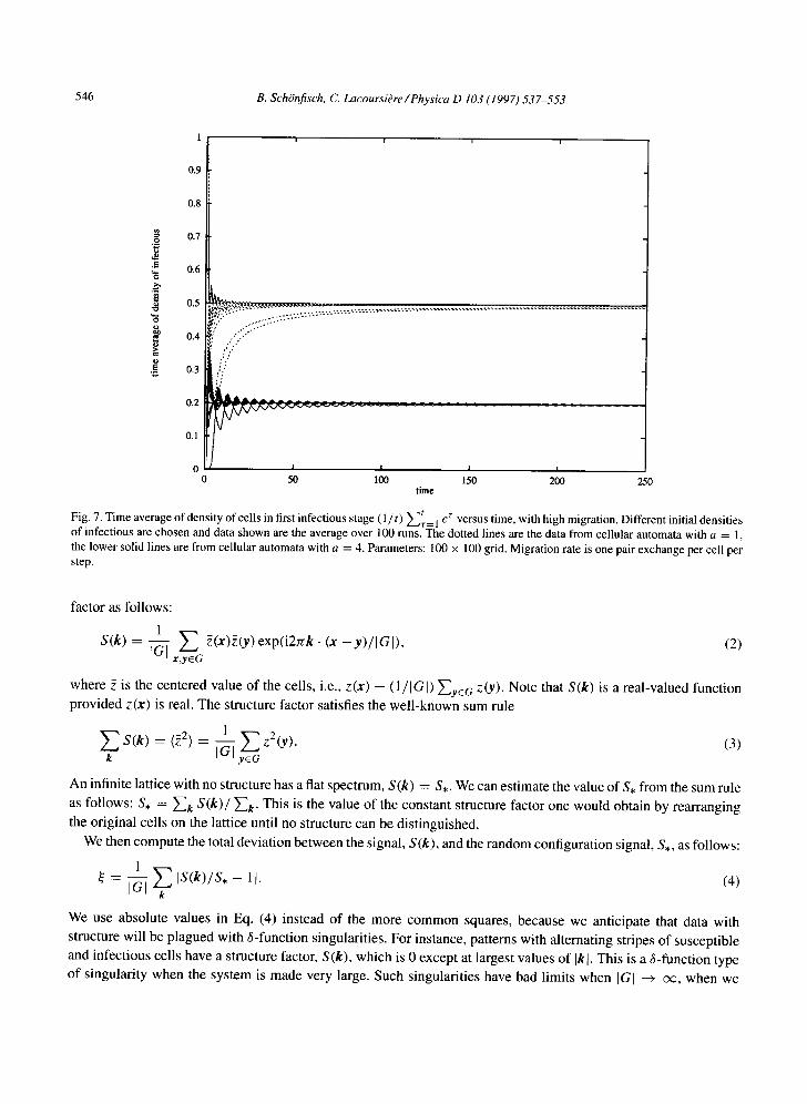
l i m t _ ~ l ( t ) = a/(a + 1). To get an estimate for O a for the automaton with high migration, we look at Da (t) as a function of t. Fig. 7 shows

averages over 100 runs for t = 0 . . . . . 52 for the automata with one and with four infectious stages. As in the case

of zero migration, Da (t) approaches 1/(a + 1), independently of the initial density of infectious cells. Note that

when the initial density is very high, or very low, Da (t) takes a long time to reach its asymptotic value.

3. Spatial patterns

3.1. Spatial patterns evolving from different initial conditions

Our main interest lies in the effect of the migration rule on the 'natural ' patterns which emerges from the cellular

automata without migration. In order to follow what happens, we need a scalar quantifier which is independent of

system size, approaches unity when the natural structure of the non-migrating automata is present, and decays to 0

when the patterns on the lattice are essentially indistinguishable from white noise. We first compute the structure

546 B. Sch6nfisch, C. Lacoursibre / Physica D 103 (1997) 537-553

I i i !

o

0.9

0.8

0.7

0.6

0.5 ~,~..-~. a .~.~ ~.,~, ~: .........

i!" .,?',':::': .... 0.4 ,," ,," ; ' , . "

0.3 ::/

0.2 ~ A ~ A . . . . . . . . . . . . . . . . . . ~ . . . . .

0 . 1 ~

0 I i i 0 50 100 150 200

time 250

Fig. 7. Time average of density of cells in first infectious stage (1/ t ) ~ t r = 1 c r versus time, with high migration. Different initial densities of infectious are chosen and data shown are the average over 100 runs. The dotted lines are the data from cellular automata with a = 1, the lower solid lines are from cellular automata with a = 4. Parameters: 100 × 100 grid. Migration rate is one pair exchange per cell per step.

factor as follows:

1 S(k) = ~ ~ ~(x)~(y) exp(i2rrk. (x -y) / IGI) , (2)

x,ycG

where ~ is the centered value of the cells, i.e., z(x) - (1/[Gi) ~-~ycG Z(y). Note that S(k) is a real-valued function provided z(x) is real. The structure factor satisfies the well-known sum rule

1 ~k S(k) = (~2) = -(~l y~GZ2(Y). (3)

An infinite lattice with no structure has a fiat spectrum, S(k) = S,. We can estimate the value of S, from the sum rule

as follows: S, = ~-~k S(k) /~k" This is the value of the constant structure factor one would obtain by rearranging the original cells on the lattice until no structure can be distinguished.

We then compute the total deviation between the signal, S(k), and the random configuration signal, S,, as follows:

1 = -~1 ~ IS(k)/S, - 1 I. (4)

k

We use absolute values in Eq. (4) instead of the more common squares, because we anticipate that data with

structure will be plagued with g-function singularities. For instance, patterns with alternating stripes of susceptible and infectious cells have a structure factor, S(k), which is 0 except at largest values of Ikl. This is a g-function type

of singularity when the system is made very large. Such singularities have bad limits when J GI ~ cx~, when we

B. Schgnfisch, C. LacoursiOre/Physica D 103 (1997) 53~553 547

0.8

0.7

0.6

0.5

0.4

0.3

0.2

0.1

0

i

0.8

0.6

30 0.2 4O 0

50

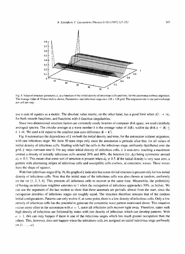
Fig. 8, Value of structure parameter, s e, as a function of the initial density of infectious cells and time, lbr the automaton without migration. The average value of 10 runs each is shown. Parameters: one infectious stage on a 128 x 128 grid. The migration rate is one pair exchange per cell per step.

use a sum of squares as a metric. The absolute value metric, on the other hand, has a good limit when ]G] -+ w ,

for both smooth functions, and functions with g-function singularities.

Since two-dimensional structure factors are extremely costly in terms of computer disk space, we used circularly

averaged spectra. The circular average at a wave number k is the average value of S(k), within the disk k _< Ik[ _<

k + 3k. We used a 6k equal to the smallest non-zero difference Ik - k'l.

Fig. 8 summarizes the dependence of ~ on both the initial density and time, for the automaton without migration,

with one infectious stage. We show 50 time steps only since the automaton is periodic after that, for all values of

initial density of infectious cells. Starting with half the cells in the infectious stage, uniformly distributed over the

grid, ~ stays constant near 0. For any other initial density of infectious cells, ~ is non-zero, reaching a maximum

around a density of initially infectious cells around 20% and 80%, the function ~(t, do) being symmetric around

do ---- 0.5. This means that some sort of structure is present when do :~ 0.5. If the initial density is very near zero, a

pattern with alternating stripes of infectious cells and susceptible cells evolves, in concentric waves. These waves

have the shape of squares.

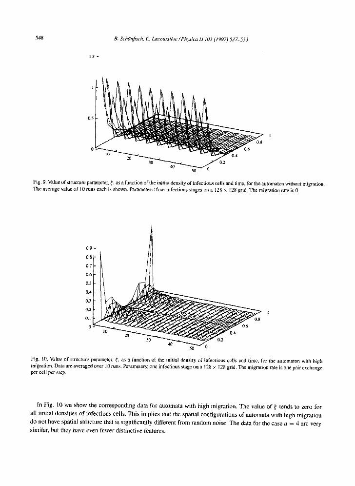
With four infectious stages (Fig. 9), the graph o f f indicates that a non-trivial structure is present only for low initial

density of infectious cells. Note that the initial state of the infectious cells was also chosen at random, uniformly

on the set { 1,2, 3, 4}. This prevents all infectious cells to recover at the same time. Meanwhile, the probability

~f having an infectious neighbor saturates to 1 when the occupation of infectious approaches 50%, as before. We

can use the argument of the last section to show that these automata are periodic almost from the start, since the

occupation densities of infectious stages are roughly equal. The structure therefore remains that of the random

initial configurations. Patterns can only evolve if, at some point, there is a low density of infectious cells. Only a low

density of infectious cells has the potential to generate the concentric wave pattern mentioned above. This situation

occurs more often in the automaton with a = 1, since all infectious cells recover right away. Therefore, states with high density of infectious are followed by states with low density of infectious which can develop patterns. With ~1 > 1. this can only happen if there is one of the infectious stages which has much greater occupation than the

others. This, however, does not happen when the infectious cells are assigned an initial infectious stage uniformly

on 11 . . . . . . } .

548 B. SchOnfisch, C. Lacoursikre / Physica D 103 (1997) 537-553

1~5 -

0,5

i

08

10

Fig. 9. Value of structure parameter, ~, as a function of the initial density of infectious cells and time, for the automaton without migration, The average value of l0 runs each is shown. Parameters: four infectious stages on a 128 × 128 grid. The migration rate is 0.

0 . 9 -

0 . 8 -

0.7

0.6

0,5

0.4

,3

,2

~1 0,8

0 04 0.6

50 "

0.3

0.2

0.1

Fig. 1O, Value of structure parameter, ~, as a function of the initial density of infectious cells and time, for the automaton with high migration, Data are averaged over 10 runs, Parameters: one infectious stage on a 128 x 128 grid. The migration rate is one pair exchange per cell per step.

In Fig. I0 we show the corresponding data for automata with high migration, The value o f ~ tends to zero for

all initial densities o f infectious cells. This implies that the spatial configurations of automata with high migration

do not have spatial structure that is significantly different from random noise. The data for the case a = 4 are very

similar, but they have even fewer dist inctive features.

B. SchOnfisch, C. Lacoursibre / Physica D 103 (1997) 537-553 549

4. S c a l i n g

A scaling law is a symmetry between variables that describe a system. For instance, a function f ( x , y) is a

scaling law for a physical system with two parameters if f ( x , y) ----- Ax~y ~, where A is a constant, since then

J(x , ~.y) = )~[~f(x, y), and similarly for x, f ( k x , y) = k~ f ( x , y). This means that the behavior of the system at

the point (x, y) is the same as at the point (x', y ' ) up to a scale factor. This sort of relationship is very natural in

physics as is demonstrated by dimensional analysis. It also shows up in non-trivial ways in, for instance, percolation

phenomena [13]; as well as in static second-order phase transition [8]; dynamic first-order phase transitions [11],

and other fields. In general, as demonstrated by Barenblatt [2,3], non-trivial scaling is strongly linked to power

law asymptotes, one of the simplest non-analytic behaviors a function can have. Cellular automata are not physical

systems, and thus one cannot apply dimensional analysis to them to demonstrate the existence of scaling. However,

there is no a priori reason to think that there is no scale invariance symmetry in these systems. In fact, if they are to

be useful at all, cellular automata must be able to model the physical realities which have scale invariance symmetry.

In the current context, the main parameters of the model, once the local function and the migration rule are

chosen, are the time t, and the effective migration rate rh(m). These parameters control two time scales namely, the

number of migration moves performed per cell, and the number of applications of the local rule to each cell. If the

local rule were trivial, i.e., if each point were to be independent of its neighbors, there would be perfect symmetry

between t and rh(m). This would mean that all global quantifiers on the lattice would be functions of t. rh(m)

only. Systems with high effective migration, th(m), at time t, would be identical to systems with lower migration,

rh(m)' = ~h(m) /k , a t l a t e r t i m e t ' = kt .

t.2

0.8

0.6

0.4

0.2

0 0

i !

8x8 - - 16x 16 . . . . . 32x32 . . . . . 64x64 ..........

128x128 . . . . . 256x256 . . . . 512x512 .. . . . .

t',

! ~ , ,

.~ ~ .,,.

' 1 % ' x ~,.

\ .,',, .;,

\ '.,.,.-,:,,

' " .)'L,

"., %-,"2Z ,, h . . . . -

"" , , ~ , :' '_~: . . . . . . k~,. .. ... ;~.:~- .......

t . . . . . I I I I I I I I I

0 . 2 0 . 4 0 . 6 0 . 8 1 1 ,2 1 .4 1 .6 1 .8 2 Rescaled time : t/IGI

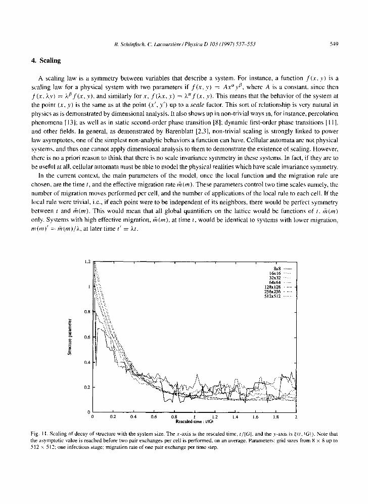
Fig. 11. S c a l i n g o f d e c a y o f s t ruc tu re w i t h the s y s t e m size . T h e x - a x i s is the r e s c a l e d t ime , t/IGI, and the y - a x i s is ~ ( t , qGI). N o t e tha t

the a s y m p t o t i c v a l u e is r e a c h e d b e f o r e t w o pa i r e x c h a n g e s p e r ce l l is p e r f o r m e d , on an a v e r a g e . P a r a m e t e r s : g r id s izes f r o m 8 x 8 up to

512 x 512 ; one in fec t ious s tage ; m i g r a t i o n ra te o f one pa i r e x c h a n g e pe r t i m e step.

550 B. SchOnfisch, C. Lacoursikre /Physica D 103 (1997) 537-553

250000

200000

150000

100000

50000

i i

t : 8.26e+03 data - - t : 8.26¢+03 white noise -

t : 1.65e+04data t : 1.65e+04 white noise

0 0.2 0.4 0.6 0.8 w a v e ntlmber

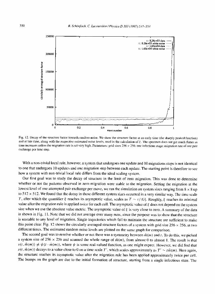
Fig. 12. Decay of the structure factor towards random noise. We show the structure factor at an ear ly t ime (the sharply peaked function)

and at late time, a long wi th the respect ive es t imated noise levels, used in the calcula t ion of s e. The spect rum does not get much flatter as

t ime increases unless the migra t ion rate is set very high. Parameters: grid sizes 256 × 256: one infect ious stage; migrat ion rate of one pair exchange per t ime step.

With a non-trivial local rule, however, a system that undergoes one update and 10 migrations steps is not identical

to one that undergoes 10 updates and one migration step between each update. The starting point is therefore to see

how a system with non-trivial local rule differs from the ideal scaling system.

Our first goal was to study the decay of structure in the limit of zero migration. This was done to determine

whether or not the patterns observed in zero migration were stable to the migration. Setting the migration at the

lowest level of one attempted pair exchange per move, we ran the simulation on system sizes ranging from 8 × 8 up

to 512 x 512. We found that the decay in these different system sizes occurred in a very similar way. The time scale

T, after which the quantifier ~ reaches its asymptotic value, scales as T ~ t / lG[. Roughly, ~ reaches its minimal

value after the migration rule is applied twice for each cell. The asymptotic value of ~ does not depend on the system

size when we use the absolute value metric. The asymptotic value of ~ is very close to zero. A summary of the data

is shown in Fig. 11. Note that we did not average over many runs, since the purpose was to show that the structure

is unstable to any level of migration. Single trajectories which fail to maintain the structure are sufficient to make

this point clear. Fig. 12 shows the circularly averaged structure factors of a system with grid size 256 × 256, at two

different times. The estimated random noise levels are plotted on the same graph for comparison.

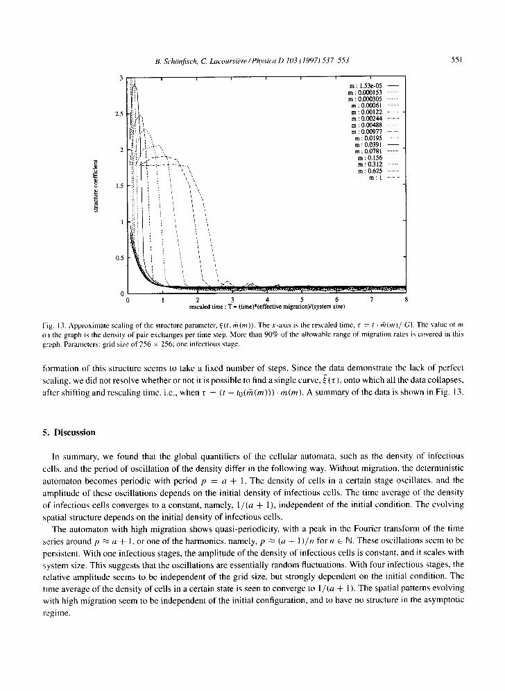
The second goal was to resolve whether or not there was a symmetry between rh(m) and t. To do this, we picked

a system size of 256 x 256 and scanned the whole range of rh(m), from almost 0 to almost I. The result is that

s(t , rh(m)) ~ 7t ( t . rh(m)), where 7t is some real-valued function, as one might expect. However, we did find that

s(t, rh(m)) decays to a value close to 0 on a time scale T' , which scales approximately as T' ~ trh(m). Here again,

the structure reaches its asymptotic value after the migration rule has been applied approximately twice per cell.

The humps on the graph are due to the initial formation of structure, starting from a single infectious state. The

B. SchOnfisch, C. Lacoursibre/Physica D 103 (1997) 537-553 551

2.5

1 .5

0 . 5

: i !

I | I I I

. i ' , ,

..,......;........

' I '. "..

.,i--.7- ~ ' - , - .~ - . - ; - . - . ~ . - . - .~ ~ . ,

i , . t .

i

i i

m : 1 . 5 3 e - 0 5 - - m : 0 . 0 0 0 1 5 3 . . . . . m : 0 . 0 0 0 3 0 5 . . . . .

m : 0 . 0 0 0 6 1 .......... m : 0.00122 .....

m : 0 . 0 0 2 4 4 . . . . . m : 0.00488 . . . . . m : 0 . 0 0 9 7 7 . . . . . .

m : 0 . 0 1 9 5 . . . . . . m : 0 . 0 3 9 1 - - m : 0 . 0 7 8 1 . . . . .

m : 0 . 1 5 6 . . . . . m : 0 . 3 1 2 .......... m : 0 . 6 2 5 . . . . .

m : l . . . . .

', ~

1 2 3 4 5 6 7 rescaled time : T - (time)*(effective migration)/(system size)

Fig. 13. Approximate scaling of the structure parameter, e(t, ffl (m)). The x-axis is the rescaled time, r = t . rh (m)/ lG[ . The value of m on the graph is the density of pair exchanges per time step. More than 90% of the allowable range of migration rates is covered in this graph. Parameters: grid size of 256 x 256; one infectious stage.

formation of this structure seems to take a fixed number of steps. Since the data demonstrate the lack of perfect

scaling, we did not resolve whether or not it is possible to find a single curve, ~ (r) , onto which all the data collapses,

after shifting and rescaling time, i.e., when r = (t - to(rh(m))) • rh(m). A summary of the data is shown in Fig. 13.

5. Discussion

In summary, we found that the global quantifiers of the cellular automata, such as the density of infectious

cells, and the period of oscillation of the density differ in the following way. Without migration, the deterministic

automaton becomes periodic with period p = a + 1. The density of cells in a certain stage oscillates, and the

amplitude of these oscillations depends on the initial density of infectious cells. The time average of the density

of infectious cells converges to a constant, namely, l / ( a + 1), independent of the initial condition. The evolving

spatial structure depends on the initial density of infectious cells. The automaton with high migration shows quasi-periodicity, with a peak in the Fourier transform of the time

series around p ~ a + 1, or one of the harmonics, namely, p ~ (a + l ) / n for n c I~. These oscillations seem to be

persistent. With one infectious stages, the amplitude of the density of infectious cells is constant, and it scales with

system size. This suggests that the oscillations are essentially random fluctuations. With four infectious stages, the relative amplitude seems to be independent of the grid size, but strongly dependent on the initial condition. The time average of the density of cells in a certain state is seen to converge to l / ( a + 1). The spatial patterns evolving

with high migration seem to be independent of the initial configuration, and to have no structure in the asymptotic

regime.

552 B. Sch6nfisch, C. Lacoursibre /Physica D 103 (1997) 537-553

Other studies lead us to think that the behavior of automata with other thresholds g may be much more complex.

The introduction of immune stages, however, is believed to have little effect on the general behavior.

The spatial structure found in automata without migration is destroyed by migration, even at the lowest pos-

sible level. The decay of the structure is found to scale with system size, i.e., se(t, IGI, ph(m)) ~ t /[GI, where

s e (t, I GI, rh (m)) is a scalar measure of the amount of structure in the system. This scaling relation indicates that all

system sizes, at all levels of migration eventually decay to 0 structure. However, the decay of the structure does not scale as se(t, IG[, rh(m)) ~ trh(m).

From a dynamical system interpretation, trajectories of the deterministic cellular automata through their state

space are not stable, in the sense that even the smallest perturbations lead to trajectories with very different properties.

This arises from the repeated application of a small perturbation.

The simulations also clearly demonstrate that the transitory regime towards configurations with almost no spatial

structure can be quite long. Our rough estimate is that one has to wait until the migration rule has been applied at

least twice for each cell in the lattice on average. In low migration rate, this leads to very long transition times, and

opens up the question of characterizing the transitory regime.

The infinite range migration rule we used destroys the locality of cellular automata. With uniform mixing, i.e.,

in the high migration regime, the structure disappears. This is one of the conditions for accuracy of the mean field

approximation. Further studies are necessary to estimate the deviations from mean field behavior. Finite range

migration rules may have different effects on the dynamics. In particular, diffusive-like migration rules may not

destroy all spatial patterns, since they can turn cellular automata into diffusion-reaction systems. The works of

DeRoos et al. [7], and Boccara et al. [6], indicate fundamentally different behavior in cellular automata with

migration rules different from ours.

Understanding of the cross-over from short range to long range, to infinite range migration rules, requires further

investigation.

Acknowledgements

Michael C. Mackey introduced the authors to each other and greatly helped the collaboration. Both authors had

useful discussions with him. He also provided travel allowances, from his FCAR (for BS) and NSERC (for CL)

grants. CL was supported for this work by a grant from NSERC in Canada, and one from SFB 382 in Germany.

Theresa L. Peszle contributed her expert editing to this text.

References

[1] J.-E Allouche and C. Reder, Oscillations spatio-temporelles engendr6es par un automate cellulaire, Discrete Appl. Math. 8 (1984) 215-254.

[2] G.I. Barenblatt, Similarity, Self-similarity, and Intermediate Asymptotics (Consultants Bureau, New York, 1979). [3l G.I. Barenblatt, Scaling, Dimensional Analysis and Intermediate Asymptotics (Cambridge University Press, New York, 1994). [4l N. Boccara and K. Cheong, Automata network SIR models for the spread of infectious diseases in populations of moving individuals,

J. Phys. A 25 (1992) 2447-2461. [5] N. Boccara, K. Cheong and M. Oram, A probabilistic automata network epidemic model with births and deaths exhibiting cyclic

behaviour, J. Phys. A 27 (1994) 1585-1597. 16] N. Boccara, O. Roblin and M. Roger, Route to chaos for a global variable of a two-dimensional 'game-of-life type' automata network,

J. Phys. A 27 (1994) 8039-8047. [7] A.M. DeRoos, E. McCauley and W.G. Wilson, Mobility versus density-limited predator-prey dynamics on different spatial scales,

Proc. Roy. Soc. London Ser. B 246 (1991) 117-122. [8] N. Goldenfeld, Lectures on phase transitions and the renormalization group, Frontiers in Physics, Vol. 85 (Addison-Wesley, Reading,

MA, 1992).

B. Sch6nfisch, C. LacoursiOre /Physica D 103 (1997) 537-553 553

[9] J.M. Greenberg, C. Greene and S. Hastings, A combinatorial problem arising in the study of reaction-diffusion equations, SIAM J. Algebraic and Discrete Methods 1 (1980) 34-42.

[10] J.M. Greenberg and S.E Hastings, Spatial patterns for discrete models of diffusion in excitable media, SlAM J. Appl. Math. 34 ( 1978) 515-523.

[ 11] J.D. Gunton, M. San Miguel and ES. Sahni, The dynamics of first-order phase transitions, in: Phase Transitions and Critical Phenomena, eds. C. Domb and J.L. Leibowitz, Vol. 8 (Academic Press, London, 1983) pp. 267-507.

I12] B. Sch6nfiscb, Propagation of fronts in cellular automata, Physica D 80 (1995) 433-450. [ 13] D. Stauffer, Introduction to Percolation Theory, 2nd Ed. (Taylor & Francis, London, Washington, DC, 1992). [14] S. Wolfram, Statistical mechanics of cellular automata, Rev. Modern Phys. 55 (1983) 601-644. I] 5] S. Wolfram, Cellular automaton fluids: Basic theory, J. Statist. Phys. 45 (1986) 471-526.