microscopic correlations in a non … correlations in a non-linear and non-perturbative n-body...

MICROSCOPIC CORRELATIONS IN A NON-LINEARAND NON-PERTURBATIVE N-BODY THEORY

M. TOMASELLIa,b, L. C. LIUc, D. URSESCUb, T. KÜHLb, S. FRITZSCHEd

a TUD-Technical University Darmstadt, D-64289 Darmstadtb GSI-Darmstadt, D-64291 Darmstadt, Germany

c Los Alamos National Laboratory, Los Alamos, NM 87545,USAd Kassel University, D-34132 Kassel, Germany

Received February 21, 2005

Energy spectra and electromagnetic transitions of nuclei are stronglyinfluenced by the correlations of the bound nucleons. Correlations are responsable forthe scattering of the valence particle to higher shell model states and for theexcitation of the shell model reference vacuum. In this work the influence of thecorrelations on the structure of open shell nuclei is analyzed. The dynamiccorrelation model we investigate is based on the unitary operator formalism which, inthis paper, is treated within a non pertubative approximation. Low lying spectracalculated for 6He, 6Li, 9Be, 13C, and 18O reproduce very well the experiments.

1. INTRODUCTION

Recently new microscopic models which depart from the classical shellmodel picture have been successfully investigated:

1) Large-basis no-core shell model have been performed in Ref. [1] andreferences therein quoted. In these calculations all nucleons are active, whichsimplifies the effective interaction to be used as no hole states are present.

2) Unstable nuclei have been successfully described by the antisymmetrizedmolecular dynamics (ADM) [2].

3) Accurate quantum Monte Carlo calculations have been performed forrealistic nuclear Hamiltonians that fit nucleon-nucleon scattering data [3].

In this work we reconsider the model presented in Refs. [4, 5] byformulating the theory within all the details needed for the numerical evaluationof the cluster coefficients presently in preparation. The model is based on amicroscopic calculation of the equation of motion method and finds easysolutions in terms of linearization approximations and cluster transformationcoefficients (CTC). In Sec. (2) we evaluate the equation of motion for twointeracting particles. The dynamic evolution of the interacting particles introducesin the model space the interaction with the shell model vacuum. In Sec. (3) wedefine the linearization approximation which has the function to reduce the

Rom. Journ. Phys., Vol. 50, Nos. 3–4 , P. 401–416, Bucharest, 2005

402 M. Tomaselli et al. 2

dimension of the active space. In Sec. (4) we introduce the cluster transformationcoefficients. These simplify the calculation of complex n-body matrix elements.In Sec. (5) we present the calculated spectra for 6Li and 18O, and for the spectraof 9Be and 13C which are calculated by using the applicaton of the present theoryto odd nuclei as given in [4].

2. THEORY OF TWO INTERACTING PARTICLES

The dynamics of two interacting particles is studied introducingcommutator equations. Assuming to write the Hamilton’s operator in secondquantization as given below:

†† †1 ( )2 intH a a v r a a a a T Vα α α α δ γβ

α αβγδ

= + αβ γδ = +∑ ∑ε (1)

and the two particle states as:

1 21 2

1 2† † †11

1 2( ) j jm m

j j JA J a a

m m M⎡ ⎤

α = ⎢ ⎥⎣ ⎦

∑ (2)

we calculate the following commutator:

1 2

1 2

1 2

1 2 1 2

1 2 † † †† †

1 2

1 2

1 2

† † † † †† †

1 ( ) , 02

1[ ] ( ) [ ] 02

j jm m

m m

j j j j

j j Ja a r a a a a a a

m m M

j j J

m m M

a a a a r a a a a a a

α α α α δ γβα αβγδ

α α α α δ γβα αβγδ

⎡ ⎤⎛ ⎞⎡ ⎤⎢ ⎥⎜ ⎟+ αβ γδ =⎢ ⎥ ⎜ ⎟⎢ ⎥⎣ ⎦ ⎝ ⎠⎣ ⎦

⎡ ⎤= ×⎢ ⎥

⎣ ⎦

⎛ ⎞⎜ ⎟× ε , + αβ γδ ,⎜ ⎟⎝ ⎠

∑ ∑ ∑

∑

∑ ∑

ε υ

υ

(3)

where the symbol in the square bracket denotes the Clebsch-Gordan’s coefficientsand where we have dropped the m’s quatum numbers in the †a ’s. By using theanticommutator relationships of the creation/annihilation operators, we calculatefor the first commutator:

1 2

1 2

1 2 1 2

1 2

1 2 † ††

1 2

1 2 † †

1 2

[ ] 0

( ) ] 0

j jm m

j j j jm m

j j Ja a a a

m m M

j j Ja a

m m M

α α αα

⎡ ⎤, =⎢ ⎥

⎣ ⎦

⎡ ⎤= +⎢ ⎥

⎣ ⎦

∑ ∑

∑

ε

ε ε

(4)

3 Microscopic correlations in a non-linear n-body theory 403

and for the second:

( )

1 2

1 2

1 2

1 1 2 22 2 1 1

1 2 † † ††

1 2

1 2

1 2

† † † † † † † †† † † †

1 ( ) [ ] 02

1 ( )2

0

j jm m

m m

j j j jj j j j

j j Jr a a a a a a

m m M

j j Jr

m m M

a a a a a a a a a a a a a a a a …

α δ γβαβγδ

αβγδ

α δ γ α γ δ α δ γ α γ δβ β β β

⎡ ⎤αβ γδ , =⎢ ⎥

⎣ ⎦

⎡ ⎤= αβ γδ⎢ ⎥

⎣ ⎦

δ + δ − δ − δ +

∑ ∑

∑ ∑

υ

υ (5)

By performing the sum over the γ and δ indices, the last equation assumesthe form:

1 2

1 2

2

1 2

2

1 2

1 2

1 2 † † ††

1 2

1 2 † ††1

1 2

1 2 † ††1

1 2

1 22

1 2

1 ( ) [ ]2

1 ( )2

1 ( )2

1 ( )2

j jm m

jm m

jm m

m m

j j Jr a a a a a a

m m M

j j Jr j a a a a

m m M

j j Jr j a a a a

m m M

j j Jr j a

m m M

α δ γβαβγδ

α δβαβδ

α β γαβγ

αβδ

⎡ ⎤αβ γδ , =⎢ ⎥

⎣ ⎦

⎛ ⎡ ⎤αβ δ += ⎜ ⎢ ⎥⎜ ⎣ ⎦⎝

⎡ ⎤+ αβ δ −⎢ ⎥

⎣ ⎦

⎡ ⎤− αβ δ⎢ ⎥

⎣ ⎦

∑ ∑

∑ ∑

∑ ∑

∑ ∑

υ

υ

υ

υ1

1

1 2

† ††

1 2 † ††2

1 2

1 ( ) ) 02

j

jm m

a a a

j j Jr j a a a a

m m M

α β δ

α β γαβγ

−

⎡ ⎤− αβ δ +…⎢ ⎥

⎣ ⎦∑ ∑ υ

(6)

Let us consider only one term of the above equation i.e. the first:

2

1 2

1 2

2

1 2 † ††1

1 2

11 2

1 12

† ††1

1 ( ) 02

12

( ) 0

i i

i

jm m

i i

iim m J M

Jj

j j Jr j a a a a

m m M

j j J j j Jj j J

m m Mm m M m m M

r j a a a a

α δβαβδ

⎡ ⎤ ⎡ ⎤α β⎢ ⎥ δ⎢ ⎥⎢ ⎥ ⎢ ⎥⎢ ⎥ ⎢ ⎥δ⎣ ⎦α βαβδ ⎣ ⎦

α β δ

⎡ ⎤αβ δ =⎢ ⎥

⎣ ⎦

⎡ ⎤= ×⎢ ⎥

⎣ ⎦

× αβ δ

∑ ∑

∑ ∑

υ

υ

(7)

In Eq. (7) we have introduced the coupled two particle matrix elementsdefined by:

11 1

1( ) ( )i

iJ i

ii

j j J j j Jr j r j

m m Mm m M

⎡ ⎤ ⎡ ⎤α β⎢ ⎥ δ⎢ ⎥⎢ ⎥ ⎢ ⎥⎢ ⎥ ⎢ ⎥δ⎣ ⎦α β⎣ ⎦

αβ δ = αβ δυ υ (8)


The three Clebsch-Gordan’s coefficients of Eq. (6):

11 2

1 12

i i

ii

j j J j j Jj j J

m m Mm m M m m M

⎡ ⎤ ⎡ ⎤α β⎢ ⎥ δ⎢ ⎥⎢ ⎥ ⎢ ⎥⎢ ⎥ ⎢ ⎥δ⎣ ⎦α β⎣ ⎦

⎡ ⎤⎢ ⎥⎣ ⎦

(9)

are not coupled in the same order as the creation/annihilation operators. If wewant therefore to associate the Clebsch’s to the operators on the right and write:

1 2

2 2

11 2 † † † †† †

1 12[[ ] [ ] ]

i i J J Jj j

ii

j j J j j Jj j Ja a a a a a a a

m m Mm m M m m M

⎡ ⎤ ⎡ ⎤α β⎢ ⎥ δ⎢ ⎥⎢ ⎥ α δ α δβ β⎢ ⎥⎢ ⎥ ⎢ ⎥δ⎣ ⎦α β⎣ ⎦

⎡ ⎤=⎢ ⎥

⎣ ⎦(10)

we have to performe some recoupling. Let us consider the first and thirdClebsch-Gordan coefficients and write:

12

12 2

12

2 2 1 2

11 2

1 12

2 1 1

2 1 11

2 1 211

2

ˆ( 1) ( 1) ˆ

ˆ ˆ( 1) ( 1)

i

r r

i

i

ij j Jj m

i

r r ij m J j jr

i r r rJ M

j j Jj j J

m m Mm m M

J j j j j JJM m m m m Mj

J j j j j J J J Jj J

j J J m m M M M

δ

⎡ ⎤δ⎢ ⎥

⎢ ⎥⎢ ⎥δ⎣ ⎦

δ+ −+

δ

δ+ + + +

δ δ

⎡ ⎤=⎢ ⎥

⎣ ⎦

⎡ ⎤ ⎡ ⎤⎡ ⎤= − − =⎢ ⎥ ⎢ ⎥⎢ ⎥ − − − − −⎣ ⎦ ⎣ ⎦⎣ ⎦

⎧ ⎫⎡ ⎤⎡ ⎤= − − ⎨ ⎬⎣ ⎦ ⎢ ⎥− − −⎩ ⎭⎣ ⎦∑

iM⎡ ⎤⎢ ⎥⎣ ⎦

(11)

In Eq. (10) the symbol in braces is the 6-J. Under the consideration that:

12ˆ

( 1) ˆr r

r ii riJ M

r ii r

J J J J J JJM M M M M MJ

⎡ ⎤+⎢ ⎥

⎢ ⎥⎢ ⎥⎣ ⎦

⎡ ⎤ ⎡ ⎤= − ⎢ ⎥ ⎢ ⎥− − ⎣ ⎦ ⎣ ⎦

(12)

we write the last equations in the following form:

2

1 2

2

11 2 † ††

1 12

12 2 11 † †1 †( 1) [[ ] [ ] ]i r

r i

i ij

ii

i r JJ j j J Jj

i rJ J

j j J j j Jj j Ja a a a

m m Mm m M m m M

J j jj J Ja a a a

J j J J

⎡ ⎤ ⎡ ⎤α β⎢ ⎥ δ⎢ ⎥⎢ ⎥ α δβ⎢ ⎥⎢ ⎥ ⎢ ⎥δ⎣ ⎦α β⎣ ⎦

⎧ ⎫⎪ ⎪+ + +⎨ ⎬ α β δ⎪ ⎪δ⎩ ⎭

⎡ ⎤=⎢ ⎥

⎣ ⎦

⎡ ⎤= − ⎢ ⎥⎣ ⎦∑(13)

Using Eq. (13) we obtain finally for the first term of Eq. (6):

2

1 2

1 2 † ††1

1 2( ) 0j

m m

j j Jr j a a a a

m m M α γβαβδ

⎡ ⎤αβ δ =⎢ ⎥

⎣ ⎦∑ ∑ υ


1 2

2

12 2 111

† ††1

( 1)

( ) [[ ] [ ] ] 0

r i

i i r

i rJ j j

i rJ J

J J J Jja

J j jj J JJ j J J

r j a a a a

⎧ ⎫⎪ ⎪+ + + ⎨ ⎬⎪ ⎪δ⎩ ⎭

α δβαβδ

⎡ ⎤= − ×⎢ ⎥⎣ ⎦

× αβ δ

∑

∑ υ(14)

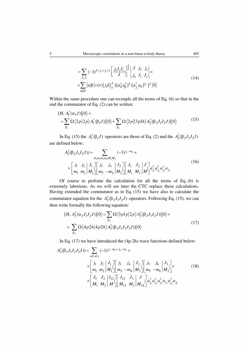
Within the same procedure one can recouple all the terms of Eq. (6) so that in theend the commutator of Eq. (2) can be written:

1 2

†11

† †1 2 1 21 2

[ ( )] 0

2 2 ( )] 0 2 3 1 ( )] 0

H A J

p p A J p p h A J J Jβ β

, α =

= Ω β + Ω β∑ ∑ (15)

In Eq. (15) the †11 ( )A Jβ operators are those of Eq. (2) and the †

2 1 22 ( )A J J Jβare defined below:

4 4

1 2 3 4 1 2

41 2 3

†2 1 22

1 2 1 3 4 2 1 2 † † †

1 2 1 3 4 2 1 2

( )) ( 1) j m

m m m m M M

jj j j

A J J J

j j J j j J J J Ja a a a

m m M m m M M M M

−β = − ×

⎡ ⎤ ⎡ ⎤ ⎡ ⎤× ⎢ ⎥ ⎢ ⎥ ⎢ ⎥−⎣ ⎦ ⎣ ⎦ ⎣ ⎦

∑(16)

Of course to perfome the calculation for all the terms of Eq. (6) isextremely laborious. As we will see later the CTC replace these calculations.Having extended the commutator as in Eq. (15) we have also to calculate the

commutator equation for the †2 1 22 ( )A J J Jβ operators. Following Eq. (15), we can

then write formally the following equation:

2

3

† †2 1 2 2 1 22 2

†3 1 2 33

[ ( )] 0 3 1 2 ( )] 0

4 2 4 2 ( )] 0

H A J J J p p p A J J J

p h p h A J J J J

β

β

, α = Ω β +

+ Ω β

∑

∑(17)

In Eq. (17) we have introduced the (4p-2h) wave functions defined below:

4 4 6 6

4 61 2 3 5

†3 1 2 33

1 2 1 3 4 2 5 6 3

1 2 1 3 4 2 5 6 3

1 2 12 12 3 † † † †

1 2 12 3 34

( )) ( 1) j m j m

all m s

j jj j j j

A J J J J

j j J j j J j j J

m m M m m M m m M

J J J J J Ja a a a a a

M M M M M M

− + −

′

β = − ×

⎡ ⎤ ⎡ ⎤ ⎡ ⎤× ×⎢ ⎥ ⎢ ⎥ ⎢ ⎥− −⎣ ⎦ ⎣ ⎦ ⎣ ⎦⎡ ⎤ ⎡ ⎤

×⎢ ⎥ ⎢ ⎥⎣ ⎦ ⎣ ⎦

∑

(18)


Within this formalism we generate a chain of commutators similar to thechain one obtains in the Green’s function mechanism. The commutator chain canbe solved perturbatively by inserting the equation for the †

2 1 22 ( )A J J Jβ term in

the †1 11 ( )A Jβ term. We prefer however to investigate a non perturbative

approximation. This can be achieved by considering that in the study of lowlying excitations of the n-body systems the higher order commutators are poorlyadmixed in the model space and therefore can be linearized. The linearization ofthe equation of motion which provides the additional model terms that areneeded in the nonperturbative approximation is illustrated in the next section.

3. THE LINEARIZATION PROCEDURE AND THE EIGENVALUE EQUATIONFOR THE DRESSED MODES

Let us start by considering the commutator:

4 4 6 6

1 2 3

†3 1 2 33

3 51 4 2 6 32 1

3 4 2 5 6 31 2 1

121 32 12

12 31 2 12

† † † ††

[ ( )] 0

( 1)

1 ( ) [2

j m j m

all m s

jj j j

H A J J J J

j j J j j Jj j J

m m M m m Mm m M

J J JJ J J

M M MM M M

r a a a a a a a a

⎡ ⎤ ⎡ ⎤⎡ ⎤− + − ⎢ ⎥ ⎢ ⎥⎢ ⎥

⎢ ⎥ ⎢ ⎥⎢ ⎥⎢ ⎥ ⎢ ⎥ ⎢ ⎥⎣ ⎦ ⎣ ⎦ ⎣ ⎦′

⎡ ⎤⎢ ⎥⎢ ⎥⎢ ⎥⎣ ⎦

α δ γβαβγδ

, α =

= − ×− −

⎡ ⎤× ×⎢ ⎥

⎢ ⎥⎣ ⎦

× αβ γδ ,

∑

∑ υ4 65

† ] 0jja a

(19)

Omitting the angular momentum algebra we have:

4 61 2 3 5

4 6 4 61 2 3 5 1 2 3 5

4 6 6 41 2 3 5 1 2 3 5

4 61 2 3 5

† † † † ††

† † † † † † † † † †† †

† † † † † † † † † ††

† † † † † †

[ ]j jj j j j

j j j jj j j j j j j j


j jj j j j j

a a a a a a a a a a

a a a a a a a a a a a a a a a a a a a a

a a a a a a a a a a a a a a a a a a

a a a a a a a a aα

α δ γβ

α δ γ α δ γβ β

α β δ γ α β δ γ

δβ

, =

= − =

= − δ +

+

4 6 6 41 2 3 5 1 2 3 5

5 4 4 5 61 2 3 6 1 2 3

† † † † † † † † † ††

† † † † † † † † † †


j j j j jj j j j j j j j

a

a a a a a a a a a a a a a a a a a a

a a a a a a a a a a a a a a a a a a …α

γ

α β δ γ α β δ γ

α δ γ δ γβ β

=

= − δ +

+ δ − + ..

(20)

The linearization is performed as in Ref. [6] by replacing in the terms of Eq. (20)pairs of creation and annhilation operators with the vacuum expectation values

5 5

† .j ja a ββ = δ In the following equation we illustrate the method by linearizing

one term of Eq. (20). We obtain:


6 4 6 5 41 2 3 5 1 2 3

6 4 6 3 4 51 2 3 5 1 2

† † † † † † † † †

† † † † † † †

j j j j jj j j j j j j

j j j j j jj j j j j j

a a a a a a a a a a a a a a

a a a a a a a a a a a a …

α δ γ α δ γβ β

α β δ γ α δ β γ

δ = δ δ −

−δ δ +δ δ + .(21)

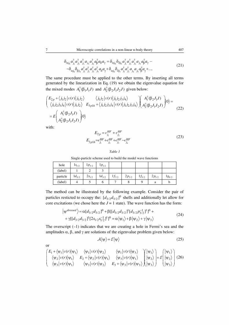
The same procedure must be applied to the other terms. By inserting all termsgenerated by the linearization in Eq. (19) we obtain the eigenvalue equation forthe mixed modes †

1 11 ( )A J Jβ and †2 1 22 ( )A J J Jβ given below:

†2 1 2 1 2 1 2 1 2 3 4 2 11

†1 2 3 4 1 2 3 1 1 2 3 4 1 2 3 4 2 1 22

†2 11

†2 1 22

( ) ( ) ( )0

( ) ( ) ( )

( )0

( )

p

p h

E j j r j j j j r j j j j A J J

j j j j r j j E j j j j r j j j j A J J J

A J JE

A J J J

⎛ ⎞+ β⎛ ⎞=⎜ ⎟⎜ ⎟⎜ ⎟⎜ ⎟+ β⎝ ⎠⎝ ⎠

⎛ ⎞β= ⎜ ⎟⎜ ⎟β⎝ ⎠

υ υυ υ

(22)

with:

1 2

1 2 3 4

2

3 1

HF HFp j j

HF HF HF HFp h j j j j

E

E

= +

= + + −

ε ε

ε ε ε ε(23)

Table 1

Single-particle scheme used to build the model wave functions

hole 1 21s / 3 21p / 1 21p /

(label) 1 2 3

particle 5 21d / 1 22s / 3 21d / 7 21 f / 3 22 p / 5 21 f / 1 22 p / 9 21g /

(label) 4 5 6 7 8 9 a b

The method can be illustrated by the following example. Consider the pair ofparticles resticted to occupy the: 0

3 2 3 2[ ]d d/ / shells and additionally let allow forcore excitations (we chose here the J = 1 state). The wave function has the form:

0 1 1 1 03 2 3 2 3 2 3 2 3 2 3 2

1 1 1 03 2 3 2 1 2 1 2 31 2

[ ] [[ ] [ ] ]

[[ ] [2 ] ]

dressed d d d d d p

d d s s

−/ / / / / /

−/ / / /

ψ = α +β +

+ γ = α ψ +β ψ + γ ψ(24)

The overscript (–1) indicates that we are creating a hole in Fermi’s sea and theamplitudes α, β, and γ are solutions of the eigenvalue problem given below:

ψ = ψA E (25)or

1 1 1 1 2 1 3 1 1

2 1 2 2 1 3 1 2 2

3 1 3 2 3 3 3 3 3

( ) ( ) ( )

( ) ( ) ( )

( ) ( ) ( )

E r r r

r E r r

r r E r

⎛ + ψ ψ ψ ψ ψ ψ ⎞⎛ ψ ⎞ ⎛ ψ ⎞⎜ ⎟⎜ ⎟ ⎜ ⎟ψ ψ + ψ ψ ψ ψ ψ = ψ⎜ ⎟⎜ ⎟ ⎜ ⎟⎜ ⎟⎜ ⎟ ⎜ ⎟ψ ψ ψ ψ + ψ ψ ψ ψ⎝ ⎠⎝ ⎠ ⎝ ⎠

Eυ υ υ

υ υ υυ υ υ

(26)


Eq. (26) is then solved with a self-consistent procedure which consists in repetedapproximations of the diagonalization method of the equation. Therefore, wehave to find a simple and expedite way to calculate the matrix elements of thetwo-body interaction in the present base and to generalize the calculation to morecomplex matrix elements. By applying the Wick’s we obtain a large number ofterms which must be additionally recoupled in order to have in the wavefunctions the same coupling scheme as in the matrix elements (see Eq. (14)).This method is to laborious. Ref. [3] solves the problem by introducing astochastic (Monte Carlo) approximation. In this paper we calculate the complexmatrix elements by introducing projection operators which are associated tounitary tensor operators as explained in the next section.

4. DEFINITION OF THE CTC FOR 3 1p h WAVE FUNCTIONS

In this section we want to formally introduce for even particles thefollowing expansion which defines the cluster transformation coefficients (CTC)of the model:

52 1 2 1 1 1 1

52 1 2 1 1 1 1

3 1 ( ) [ ] 0

( ) [ ] 0r s

r s

JJ r s r s

J J

JJ r s r s

J J

p h U J J J J J J

V J J J J J J

= α | α α | α α +

+ α | |

∑

∑ ε ε ε ε(27)

Fig. 1. – Calculated low lying energy spectra for 6He, 9Be, and 13C compared with theexperimental spectra.


where

2 1 1(3 1 ) ( ) ( )a pp h ph ppα →α α (28)

and

2 1 1(3 1 ) ( ) ( )a pp h pp phα → ε ε (29)

where the subscripts a active≡ associated to the angular momentum Jr

characterizes the active configuration and p passive≡ associated to the angularmomentum Js the passive. The definition of active and passive components hasbeen introduced to separate the matrix elements of the interaction inparticle-particle and particle-hole matrix elements respectively. In order tocalculate the CTC- 5

2 1 2 1 1( )J r sU J J J Jα | α α and 52 1 2 1 1( ),J r sV J J J Jα | ε ε let us

introduce the following operator:

† †

(2) ( 1) i i

k

i i k

J Mkm

M M m

ii iii j ji

ji k j ii i i i

j j JJ J k i i Ja a a a

m m MM M m m m M

′ ′−

′

⎡ ⎤⎡ ⎤⎢ ⎥⎢ ⎥⎢ ⎥⎢ ⎥ ′′⎢ ⎥⎢ ⎥ ′′⎣ ⎦⎣ ⎦

π = − ×

′′ ′ ⎡ ⎤× ⎢ ⎥′−′− ⎢ ⎥⎣ ⎦

∑(30)

operator which destroys and creates a particle pair and let us calculate his effecton the 3 1p h wave-function. We obtain:

4 4

1

2 2 1 2

31 14 22 1 2

13 4 21 2 1 2† † †

(2) ( ) 0 ( 1)

( 1)

i i

k

i i k

J Mkm

M M m

ii i i

j j ii k i ii i

j m

j jii j

A j J J

j j JJ J k i i J

m m MM M m m m M

j j Jj j J J J J

m m Mm m M M M M

a a a a a a

′ ′−

′

⎡ ⎤⎡ ⎤⎢ ⎥⎢ ⎥⎢ ⎥⎢ ⎥⎢ ⎥⎢ ⎥⎣ ⎦⎣ ⎦

⎡ ⎤⎡ ⎤− ⎢ ⎥⎢ ⎥

⎢ ⎥⎢ ⎥⎢ ⎥ ⎢ ⎥⎣ ⎦ ⎣ ⎦

′′

π α = − ×

′′ ′ ⎡ ⎤× ×⎢ ⎥′ ′′ ′ −− ⎢ ⎥⎣ ⎦

⎡ ⎤× − ×⎢ ⎥− ⎣ ⎦×

∑

42 3

† † 0jj ja a

(31)

Considering for the moment only the creation/annihilation algebra weobtain the following equation:

41 2 3

2 4 3 4 3 43 2 1

† † † † †

† † † † † † † † †1 1 2

j j jii j j j

j j j j j j j j ji i ii i ij j j

a a a a a a a a

a a a a a a a a a a a a exchange terms

′′

′ ′ ′′ ′ ′

=

= δ δ − δ δ + δ δ + −(32)

By using the recoupling technics we get for first three terms of Eq. (32) thefollowing expressions:


12 2

243

243

111

2

† † †

† † †1

ˆ ˆ[ ] ( 1)

[[ ] [ ] ] 0

[[ ] [ ] ] 0

r i

i

i

ii i k J J

rJ J

J J Jji i Mj

k

J J Jji i Mj

k

J k JTerm k J

J J J

J k Ja a a a

M m M

J k JCoef a a a a

M m M

′+ + + + +

′

′ ′

′ ′

⎧ ⎫= − ×⎨ ⎬′⎩ ⎭

⎡ ⎤× =⎢ ⎥′⎣ ⎦

⎡ ⎤= ⎢ ⎥′⎣ ⎦

∑

(33)

1 1 52

1 3 4 5

4 1 3 4 12 1 2

4 3 41 2 1 3 4 2

1 5 52 1 2

4

341

ˆˆ ˆ ˆ ˆ ˆ ˆ ˆ ˆ ˆ( )[ ] ( 1) r r r

r r r r r

i J J J Jr r i r r r

J J J J J

r r r r

r r r r r

r r

rk

i r

Term J J J J J J J J k J

j j J j j J i J J k J J

J J J J j J J j J J J J

i J JJ k J

i j JM m M

J J k

′ ′+ + + + +

′

′= − ×

′⎧ ⎫⎧ ⎫⎧ ⎫⎧ ⎫× ×⎨ ⎬⎨ ⎬⎨ ⎬⎨ ⎬′ ′⎩ ⎭⎩ ⎭⎩ ⎭⎩ ⎭

′⎧ ⎫⎪ ⎪′× ⎨ ⎬ ′⎪ ⎪⎩ ⎭

∑

5 3

4

5 3

4

† † †2

† † †2 2

[[ ] [ ] ] 0

[[ ] [ ] ] 0

r r

r r

J J Jji i M

J J Jji i M

k

a a a a

J k JCoef a a a a

M m M

′ ′

′ ′

⎡ ⎤=⎢ ⎥

⎣ ⎦

⎡ ⎤= ⎢ ⎥′⎣ ⎦

(34)

2

1 3 4 5

5

13 5 23

4 3 41 2 1 3 4 2

1 5 52 1 1

4

† †34 11

ˆˆ ˆ ˆ ˆ ˆ[ ] ( 1)

[[ ] [

r r

r r r r r

r

i i j J Ji r r r

J J J J J

r r r r

r r r r r

r rJ

irk

i r

Term J J J J kJ

j j J j j J i J J k J J

J J J J j J J j J J J J

i J JJ k J

i j J a aM m M

J J k

′ ′ ′+ + + +

′

′= − ×

′⎧ ⎫⎧ ⎫⎧ ⎫⎧ ⎫× ×⎨ ⎬⎨ ⎬⎨ ⎬⎨ ⎬′ ′⎩ ⎭⎩ ⎭⎩ ⎭⎩ ⎭

′⎧ ⎫⎡ ⎤⎪ ⎪′× ⎨ ⎬⎢ ⎥′⎣ ⎦⎪ ⎪

⎩ ⎭

∑

3

4

5 3

4

†

† † †3 1

] ] 0

[[ ] [ ] ] 0

r

r r

J Jji M

J J Jji i M

k

a a

J k JCoef a a a a

M m M

′ ′

′ ′

=

⎡ ⎤= ⎢ ⎥′⎣ ⎦

(35)

In Eqs. (34, 35) we have introduced in braces the 9-J symbols. We can nowto collect the three terms by using the necessary δ’s and we write:

†2 1 22

†1 2 3 2 1 22

(2) ( ) 0

( ) ( ) 0

k

km

k

A j J JM

J k JCoef Coef Coef A j J JM

M m M

π α =

⎡ ⎤ ′= + + α⎢ ⎥′⎣ ⎦

(36)


Dividing now by 1 2 3,Coef Coef Coef+ + we define unitary tensor operators [7]:

1 2 3

1(2) (2)k k

k km mCoef Coef Coef

π = π+ +

(37)

Eq. (36) means that operating with (2)k

kmπ on a wave function of the type

3 1 JMp h we obtain 3 1 J

Mp h ′ i.e., we reproduce the same wave function in a

rotated frame. Using a matrix formulation we write for Eq. (36):

†2 2 1 2 2 1 22

1 2 3

0 ( ) (2) ( ) 0

( )

k

km

k

A j J JM A j J JM

J k JCoef Coef Coef

M m M

′α π α =

⎡ ⎤= + +⎢ ⎥′⎣ ⎦

(38)

or

†2 2 1 2 2 1 220 ( ) (2) ( ) 0

k

km

k

J k JA j J JM A j J JM

M m M⎡ ⎤′α π α = ⎢ ⎥′⎣ ⎦

(39)

Analogously we introduce the operator

† †

(2) ( 1) i i j j

k

i i k

M j m j mJkm

M M m

i ii ij ii j

i j ii k i j ii

u

i j J i j JJ J ka a a a

m m M m m MM M m

′′ ′− + − + −′

′

⎡ ⎤⎡ ⎤⎢ ⎥⎢ ⎥

′⎢ ⎥ ′⎢ ⎥⎢ ⎥⎢ ⎥⎣ ⎦ ⎣ ⎦

= − ×

′ ′ ′′ ⎡ ⎤× ⎢ ⎥− ′ ′ ′′ − −− ⎢ ⎥⎣ ⎦

∑(40)

which destroys and creates a particle-hole pair. The operator algebra yields:

2 3 1 3 1 2

† † † † † † † † †1 4 2 4 3 4i j j i j j i j ji i ij j j j j ja a a a a a a a a a a a′ ′ ′ ′ ′ ′δ δ − δ δ + δ δ (41)

By considering the recoupling algebra, we derive for the three terms:

3 51 3 2

1 2 3 5

111 3 24 1 2

2 11 2 1 3 4 2

1 1 2 34 1 2

3 5

24

3

ˆˆ ˆ ˆ ˆ ˆ ˆ[ ] ( 1) r r r

r r r r r

i j j J J J J Jr r i

J J J J J

i i r r

r r r r r r r

r r

rk

r

Term J J J J J kJ

j j J j j J i j J J J J

J j J J J J k J J J j J

J J JJ k J

J j kM m M

J j J

′+ + + + + + + +

′= − ×

⎧ ⎫⎧ ⎫⎧ ⎫⎧ ⎫× ×⎨ ⎬⎨ ⎬⎨ ⎬⎨ ⎬′ ′ ′⎩ ⎭⎩ ⎭⎩ ⎭⎩ ⎭⎧ ⎫

⎡ ⎤⎪ ⎪× ⎨ ⎬⎢ ′⎣ ⎦⎪ ⎪′⎩ ⎭

∑

3 5

3 5

† † †2 3

† † †4 2 3

[[ ] [ ] ] 0

[[ ] [ ] ] 0

r r

r r

J J Jji M

J J Jji M

k

a a a a

J k JCoef a a a a

M m M

′

′

=⎥

⎡ ⎤= ⎢ ⎥′⎣ ⎦

(42)


1 2 1

3 5

5 4 1 2

† † †5 1 3

( 1) ( )

[[ ] [ ] ] 0r r

j j J

J J Jji M

k

Term Term with j j

J k JCoef a a a a

M m M

+ −

′

= ∗ − →

⎡ ⎤= ⎢ ⎥′⎣ ⎦

(43)

3 4 1

1

1

1 21261

† † †1 2

† † †6 1 2

ˆ ˆ[ ] ( 1)

[[ ] [ ] ] 0

[[ ] [ ] ] 0

i

r i

i

i

ij j k J J

rJ J

JJ Jji M

k

JJ Jji M

k

J k JTerm kJ

J J J

J k Ja a a a

M m M

J k JCoef a a a a

M m M

+ + + + +

′

′

′

⎧ ⎫= − ×⎨ ⎬′⎩ ⎭

⎡ ⎤× =⎢ ⎥′⎣ ⎦

⎡ ⎤= ⎢ ⎥′⎣ ⎦

∑

(44)

Collecting the three terms by using the necessary δ’s, like done for the πoperator, we write:

†2 1 22

†4 5 6 2 1 22

(2) ( ) 0

( ) ( ) 0

k

km

k

u A j J JM

J k JCoef Coef Coef A j J JM

M m M

α =

⎡ ⎤ ′= + + α⎢ ⎥′⎣ ⎦

(45)

Also here, dividing by 4 5 6Coef Coef Coef+ + we define unitary tensor operators:

4 5 6

1(2) (2)k k

k km mu u

Coef Coef Coef=

+ +(46)

It is easy now to verify that the commutator of two π’s is given by:

1 2

1 2

1 2

1 2

11 2 2

3

[ (2) (2)]

ˆˆ(1 ( 1) ) [ ] (2)

k k k

k

k k km m m

i rk k k km

k k k r

k k k J k Jj k

m m m j j J

⎡ ⎤⎢ ⎥+ −⎢ ⎥⎢ ⎥⎣ ⎦

π , π =

⎧ ⎫= − − π⎨ ⎬′⎩ ⎭

(47)

Owing to the orthogonal relationships holding between the defined A2 operators,

the 2(2 1)J + matrices given in Eq. (39) are linear independent. It follows thereforethat the structure defined by Eq. (46) is that of a full linear group in (2J + 1)dimension and of its unitary subgroup U2J+1. The calculation of the transformationcoefficients is now reduced to the construction of .

iCoefλ In order to demonstrate

this, let us now operate with the Casimir’s operator of the group †(( (2))k

kmπ ⊗

(2))k

km⊗π on Eq. (27). We obtain:

† †2 1 2 2 12 ( ) ( (2)) (2)) ( )

i jk k

k km mA J J A J J Coef Coefλ λα π ⊗π α = (48)


where the double bar matrix elements have been introduced because the CTC areindependent from the m’s quantum numbers and where the subindex λi classifiesthe three different partitions spanned by the wave functions. On the other handwe can write:

(2) (1 )k k

k km m

i

iπ = π ,∑ (49)

where the sum is running over all the possible partitions. By applying now:

† †(( (2)) (2)) ( (1 )) ( (1 ))k k k k

k k k km m m m

i

i iπ ⊗π = π , ⊗ π ,∑ (50)

to †2 12 ( )A J Jα we obtain:

† †2 2 2 2 12

†5 52 1 1 1 2 1 1 1

( ) ( (1 )) ( (1 )) ( )

( ) ( )

k k

k km m

r s J r sJ

A J j i i A J j

V J J J V J J J

α π , ⊗ π , α =

= α | α |ε ε ε ε(51)

Equating Eq. (48) and Eq. (51) we obtain the following matrix:

4

4

4

† † †31 1 1 2 1 3

† † †22 1 2 2 2 3

† † †3 1 3 2 3 3 1

( [ ] [ ] )

( [ ] [ ] )

( [ ] [ ] )

sr

sr

sr

JJ Jjii

JJ Jji i

JJ Jji i

a a a aCoef Coef Coef Coef Coef Coef

Coef Coef Coef Coef Coef Coef a a a a

Coef Coef Coef Coef Coef Coef a a a a

⎛ ⎞ ′⎜ ⎟⎜ ⎟⎜ ⎟ ′⎜ ⎟⎜ ⎟⎝ ⎠ ′

⎛ ⎞|∗ ∗ ∗ ⎜ ⎟∗ ∗ ∗ |⎜ ⎟

⎜ ⎟∗ ∗ ∗ ⎜ ⎟|⎝ ⎠†5 5

2 1 1 1 1 1 1 2 1 1 1 1 1 1

†5 52 1 2 1 1 1 1 2 1 2 1 1 1 1

†5 52 1 3 1 1 1 1 2 1 3 1 1 1 1

( ) ) ( ) )

( ) ) ( ) )

( ) ) ( ) )

r s r s J r s r sJ

r s r s J r s r sJ

r s r s J r s r sJ

V J J J J J V J J J J J



=

⎛ ⎞α | λ | α | λ |⎜ ⎟⎜= α | λ | α | λ |⎜⎜ α | λ | α | λ |⎝ ⎠

ε ε ε ε ε ε ε ε



4

4

4

† † †3

† † †2

† † †1

( [ ] [ ] )

( [ ] [ ] )

( [ ] [ ] )

sr

sr

sr

JJ Jjii

JJ Jji i

JJ Jji i

a a a a

a a a a

a a a a

′

′

′

⎟ ⋅⎟⎟

⎛ ⎞|⎜ ⎟⋅ |⎜ ⎟⎜ ⎟⎜ ⎟|⎝ ⎠

(52)

which defines the CTC 52 1 1 1 1( )J r sV J J Jα | λ α α of Eq. (27). Analogous eigenvalue

equation can be written for the CTC arising from the h operators. Within theCTC, from Eq. (52) and those for the U’s not given explicitly, we can calculatethe matrix elements of the nuclear interaction using Eq. (27). We obtain thefollowing results:

†5 52 1 2 1 1 2 1 2 1 1

3 1 ( ) 3 1

( ) ( )i r s j r s

i r s J j r sJJ J J J

p h r p h

U J J J J U J J J J′ ′λ λ

=

′ ′= α | λ α α α | λ α α ×∑υ


1 1 1 1

†5 52 1 2 1 1 2 1 2 1 1

1 1 1 1

†5 52 1 2 1 1 2 1 2 1 1

[ ] ( ) [ ]

( ) ( )

[ ] ( ) [ ]

( ) ( )

i r s j r s

i r s j r

J Ji r s j r s

i r s J j r sJJ J J J

J Ji r s j r s

i r s J j r sJJ J J

i

J J r J J

V J J J J V J J J J

J J r J J

U J J J J U J J J J

′ ′µ µ

′λ λ

′ ′× λ α α λ α α +

′ ′+ α | µ ε α | µ ε ×

′ ′× µ ε µ ε =

′= α | λ α α α | λ α α ×

× λ α

∑

∑

ε ε

ε ε

υ

υ

1 1

†5 52 1 2 1 1 2 1 2 1 1

1 1

( )

( ) ( )

( )i r s j r

r j r

i r s J j r sJJ J J

i r j r

J r J

V J J J J V J J J J

J r J

′µ µ

′λ α +

′+ α | µ ε α | µ ×

′× µ µ

∑ ε ε ε

ε ε

υ

υ

(53)

Fig. 2. – Calculated spectrum of 6Li. Right: energy levels calculated by restricting theexcitation of the hole to the 1

21s state. Left: energy levels calculated by allowing the

excitation of the 32

1p -hole. Calculations given to the left reproduce the energy of the

second 1+ level and the experimental magnetic moment of the ground state µ = 2.822.

5. RESULTS

Application of the model to nuclear structure calculations requiresdetermining the single-particle energies and chosing nuclear two-bodyinteractions. The sigle-particle level used to construct the model states are givenin Table 1. The single-particle energies of these levels are taken from the


experimental level spectra of the neighbouring nuclei. For the particle-particleinteraction, we use the Yale potential [8]. For the particle-hole interaction, weuse the phenomenological potential of [9]. A comparison of the matrix elementscalculated with these interactions with those calculated with modern realisticpotentials [11, 12, 13, 14] is given in Ref. [5]. In Fig. 1 we compare thecalculated low lying spectra for 6He, 9Be, and 13C with the experiments. Anoverall good agreement with the experimental values [15] has been obtained. InFig. 2 we present two calculated spectra for 6Li. The first is calculated byallowing the model hole to be excited only from the 1

21s state. The model

dimension of 196 components is not large enough to reproduce the second 1+

level and the magnetic moment of the ground state. The second calculated with amuch larger space with dimension of 525 components includes the excitation ofthe hole also from the 3

21p state. Within this space we reproduce the energy of

the second 1+ level and the magnetic moment of the ground state. Calculation ofthe charge distribution in this space is presently investigated. Recently, a low kV −

method has been also applied to nuclear structure calculations [10, 16]. The fivelow-lying positive-parity states of 18O calculated with low kV − are compared withthe corresponding BDCM levels in Fig. 3. A very good agreement has beenfound. So far, there is no information on the high-energy sector of the 18O levelscalculated with low kV − . In Fig. 1, 2, 3 in order to be consistent with Refs. [4, 5],the theoretical results obtained for 6He, 6Li, and 18O have been labeled BDCM(boson-dynamic correlation model) and those obtained for 9Be and 13C DCM

Fig. 3. – Low-lying states of 18O calculated with Vlow–k are shown and compared withthe corresponding calculated levels.


(dynamic correlation model). To conclude in this paper we have presented adetailed treatment of the microscopic correlations. Application of the method tonuclear structure calculations is performed within linearization approximationsand cluster transformation coefficients. Within these coefficients it is possible tocalculate the complex matrix elements of the nuclear interaction which areneeded for structure calculations by using recursive formulas. In this way we canperforme expedite and exact calculations. Numerical tables for the CTC will beavailable soon.

REFERENCES

1. P. Navratil and B. R. Barret, Phys Rev. C57, 3119 (1998).2. Y. Kanada-En’yo and Horiuchi, Phys. Rev. C555, 2860 (1997).3. S. C. Pieper and R. B. Wiringa, Ann. Rev. Part. Sci. 51, 53 (2001).4. M. Tomaselli, L. C. Liu, S. Fritzsche, T. Kühl, and D. Ursescu, Nucl. Phys. A738, 216 (2004).5. M. Tomaselli, L. C. Liu, S. Fritzsche, and T. Kühl, J. Phys. G: Nucl. Part. Phys. 30, 999 (2004).6. G. E. Brown, Unified Theory of Nuclear Models, Amsterdam: North-Holland (1964).7. G. Racah, Group theory and spectroscopy, CERN Report 61-8, Geneve, Schwitzerland (1961).8. C. M. Shakin, Y. R. Wagmare, M. Tomaselli, and, M. H. Hull, Phys. Rev. 1 61, 1015 (1967).9. D. J. Millener and D. Kurath, Nucl. Phys. 255, 315 (1975).

10. L. Coraggio, A. Covello, A Gargano, N. Itaco, T. T. S. Kuo, D. R. Entem, and L. Machleidt,Phys. Rev. C66, 021303(R) (2002).

11. B. H. Wildenthal, Prog. Part. Nucl. Phys. 11, 5 (1984).12. M. F. Jiang, R. Machleidt, D. B. Stout, and T. T. S. Kuo. Phys. Rev. C46, 910 (1992).13. M. Lacombe, B. Loiseau. J. M. Richard, R. Vinh Mau, J. Côté, P. Pirès, and R. de Tourreil,

Phys. Rev. C21, 861 (1980).14. R. Machleidt, Adv. Nucl. Phys. 19, 189 (1989).15. F. Ajzenberg-Selove, Nucl. Phys. A413, 1 (1984), A433, 1 (1985), A449, 1 (1986), A460,

1 (1986), A490, 1 (1988).16. S. Bogner, T. T. S. Kuo, L. Coraggio, A. Covello, and N. Itaco, Phys. Rev. C65, 051301(R)

(2002).

microscopic correlations in a non … correlations in a non-linear and non-perturbative n-body...

Documents