micropower system modeling with homer - pspb.org · chapter 15 micropower system modeling with...

CHAPTER 15

MICROPOWER SYSTEM MODELINGWITH HOMER

TOM LAMBERTMistaya Engineering Inc.

PAUL GILMAN and PETER LILIENTHALNational Renewable Energy Laboratory

15.1 INTRODUCTION

The HOMER Micropower Optimization Model is a computer model developed by

the U.S. National Renewable Energy Laboratory (NREL) to assist in the design of

micropower systems and to facilitate the comparison of power generation technol-

ogies across a wide range of applications. HOMER models a power system’s phy-

sical behavior and its life-cycle cost, which is the total cost of installing and

operating the system over its life span. HOMER allows the modeler to compare

many different design options based on their technical and economic merits. It

also assists in understanding and quantifying the effects of uncertainty or changes

in the inputs.

A micropower system is a system that generates electricity, and possibly heat, to

serve a nearby load. Such a system may employ any combination of electrical

generation and storage technologies and may be grid-connected or autonomous,

meaning separate from any transmission grid. Some examples of micropower sys-

tems are a solar–battery system serving a remote load, a wind–diesel system serving

an isolated village, and a grid-connected natural gas microturbine providing elec-

tricity and heat to a factory. Power plants that supply electricity to a high-voltage

transmission system do not qualify as micropower systems because they are not

Integration of Alternative Sources of Energy, by Felix A. Farret and M. Godoy Sim~ooesCopyright # 2006 John Wiley & Sons, Inc.

379

dedicated to a particular load. HOMER can model grid-connected and off-grid

micropower systems serving electric and thermal loads, and comprising any com-

bination of photovoltaic (PV) modules, wind turbines, small hydro, biomass power,

reciprocating engine generators, microturbines, fuel cells, batteries, and hydrogen

storage.

The analysis and design of micropower systems can be challenging, due to the

large number of design options and the uncertainty in key parameters, such as load

size and future fuel price. Renewable power sources add further complexity

because their power output may be intermittent, seasonal, and nondispatchable,

and the availability of renewable resources may be uncertain. HOMER was

designed to overcome these challenges.

HOMER performs three principal tasks: simulation, optimization, and sensitivity

analysis. In the simulation process, HOMER models the performance of a particular

micropower system configuration each hour of the year to determine its technical

feasibility and life-cycle cost. In the optimization process, HOMER simulates many

different system configurations in search of the one that satisfies the technical con-

straints at the lowest life-cycle cost. In the sensitivity analysis process, HOMER

performs multiple optimizations under a range of input assumptions to gauge the

effects of uncertainty or changes in the model inputs. Optimization determines

the optimal value of the variables over which the system designer has control

such as the mix of components that make up the system and the size or quantity

of each. Sensitivity analysis helps assess the effects of uncertainty or changes in

the variables over which the designer has no control, such as the average wind

speed or the future fuel price.

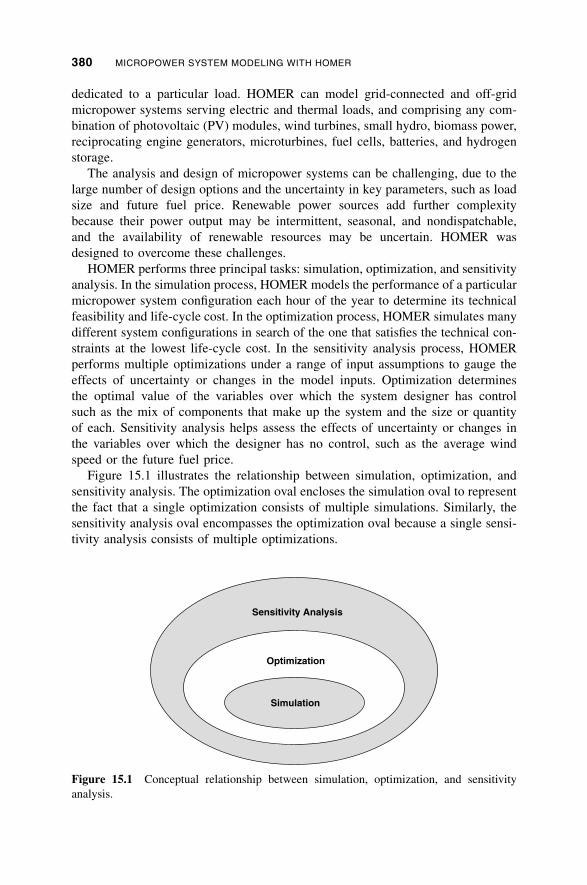
Figure 15.1 illustrates the relationship between simulation, optimization, and

sensitivity analysis. The optimization oval encloses the simulation oval to represent

the fact that a single optimization consists of multiple simulations. Similarly, the

sensitivity analysis oval encompasses the optimization oval because a single sensi-

tivity analysis consists of multiple optimizations.

Simulation

Optimization

Sensitivity Analysis

Figure 15.1 Conceptual relationship between simulation, optimization, and sensitivity

analysis.

380 MICROPOWER SYSTEM MODELING WITH HOMER

To limit input complexity, and to permit fast enough computation to make opti-

mization and sensitivity analysis practical, HOMER’s simulation logic is less

detailed than that of several other time-series simulation models for micropower

systems, such as Hybrid2 [1], PV-DesignPro [2], and PV*SOL [3]. On the other

hand, HOMER is more detailed than statistical models such as RETScreen [4],

which do not perform time-series simulations. Of all these models, HOMER is

the most flexible in terms of the diversity of systems it can simulate.

In this chapter we summarize the capabilities of HOMER and discuss the ben-

efits it can provide to the micropower system modeler. In Sections 15.2 through

15.4 we describe the structure, purpose, and capabilities of HOMER and introduce

the model. In Sections 15.5 and 15.6 we discuss in greater detail the technical and

economic aspects of the simulation process. A glossary defines many of the terms

used in the chapter.

15.2 SIMULATION

HOMER’s fundamental capability is simulating the long-term operation of a micro-

power system. Its higher-level capabilities, optimization and sensitivity analysis,

rely on this simulation capability. The simulation process determines how a parti-

cular system configuration, a combination of system components of specific sizes,

and an operating strategy that defines how those components work together, would

behave in a given setting over a long period of time.

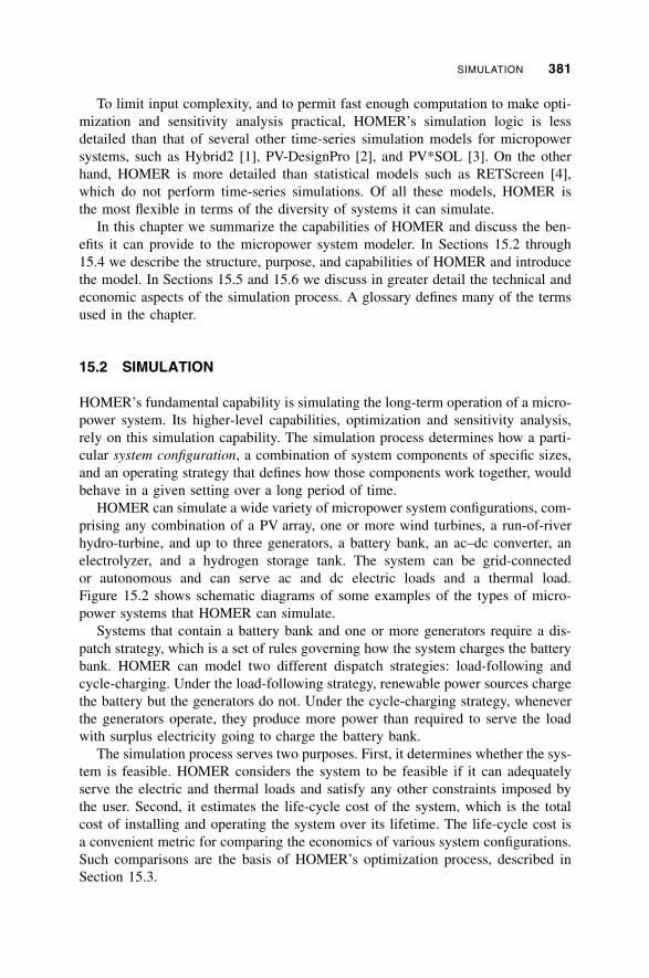
HOMER can simulate a wide variety of micropower system configurations, com-

prising any combination of a PV array, one or more wind turbines, a run-of-river

hydro-turbine, and up to three generators, a battery bank, an ac–dc converter, an

electrolyzer, and a hydrogen storage tank. The system can be grid-connected

or autonomous and can serve ac and dc electric loads and a thermal load.

Figure 15.2 shows schematic diagrams of some examples of the types of micro-

power systems that HOMER can simulate.

Systems that contain a battery bank and one or more generators require a dis-

patch strategy, which is a set of rules governing how the system charges the battery

bank. HOMER can model two different dispatch strategies: load-following and

cycle-charging. Under the load-following strategy, renewable power sources charge

the battery but the generators do not. Under the cycle-charging strategy, whenever

the generators operate, they produce more power than required to serve the load

with surplus electricity going to charge the battery bank.

The simulation process serves two purposes. First, it determines whether the sys-

tem is feasible. HOMER considers the system to be feasible if it can adequately

serve the electric and thermal loads and satisfy any other constraints imposed by

the user. Second, it estimates the life-cycle cost of the system, which is the total

cost of installing and operating the system over its lifetime. The life-cycle cost is

a convenient metric for comparing the economics of various system configurations.

Such comparisons are the basis of HOMER’s optimization process, described in

Section 15.3.

SIMULATION 381

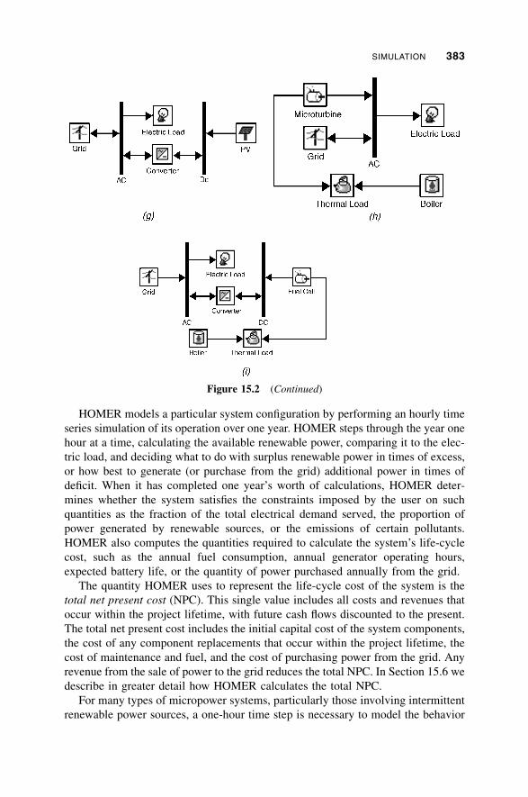
Figure 15.2 Schematic diagrams of some micropower system types that HOMER models: (a) a

diesel system serving an ac electric load; (b) a PV–battery system serving a dc electric load; (c) a

hybrid hydro–wind–diesel system with battery backup and an ac–dc converter; (d) a wind–diesel

system serving electric and thermal loads with two generators, a battery bank, a boiler, and a dump

load that helps supply the thermal load by passing excess wind turbine power through a resistive

heater; (e) a PV–hydrogen system in which an electrolyzer converts excess PV power into

hydrogen, which a hydrogen tank stores for use in a fuel cell during times of insufficient PV power;

(f) a wind-powered system using both batteries and hydrogen for backup, where the hydrogen fuels

an internal combustion engine generator; (g) a grid-connected PV system; (h) a grid-connected

combined heat and power (CHP) system in which a microturbine produces both electricity and heat;

(i) a grid-connected CHP system in which a fuel cell provides electricity and heat.

382

HOMER models a particular system configuration by performing an hourly time

series simulation of its operation over one year. HOMER steps through the year one

hour at a time, calculating the available renewable power, comparing it to the elec-

tric load, and deciding what to do with surplus renewable power in times of excess,

or how best to generate (or purchase from the grid) additional power in times of

deficit. When it has completed one year’s worth of calculations, HOMER deter-

mines whether the system satisfies the constraints imposed by the user on such

quantities as the fraction of the total electrical demand served, the proportion of

power generated by renewable sources, or the emissions of certain pollutants.

HOMER also computes the quantities required to calculate the system’s life-cycle

cost, such as the annual fuel consumption, annual generator operating hours,

expected battery life, or the quantity of power purchased annually from the grid.

The quantity HOMER uses to represent the life-cycle cost of the system is the

total net present cost (NPC). This single value includes all costs and revenues that

occur within the project lifetime, with future cash flows discounted to the present.

The total net present cost includes the initial capital cost of the system components,

the cost of any component replacements that occur within the project lifetime, the

cost of maintenance and fuel, and the cost of purchasing power from the grid. Any

revenue from the sale of power to the grid reduces the total NPC. In Section 15.6 we

describe in greater detail how HOMER calculates the total NPC.

For many types of micropower systems, particularly those involving intermittent

renewable power sources, a one-hour time step is necessary to model the behavior

Figure 15.2 (Continued)

SIMULATION 383

of the system with acceptable accuracy. In a wind–diesel–battery system, for exam-

ple, it is not enough to know the monthly average (or even daily average) wind

power output, since the timing and the variability of that power output are as impor-

tant as its average quantity. To predict accurately the diesel fuel consumption, diesel

operating hours, the flow of energy through the battery, and the amount of surplus

electrical production, it is necessary to know how closely the wind power output

correlates to the electric load, and whether the wind power tends to come in long

gusts followed by long lulls, or tends to fluctuate more rapidly. HOMER’s one-hour

time step is sufficiently small to capture the most important statistical aspects of the

load and the intermittent renewable resources, but not so small as to slow computa-

tion to the extent that optimization and sensitivity analysis become impractical.

Note that HOMER does not model electrical transients or other dynamic effects,

which would require much smaller time steps.

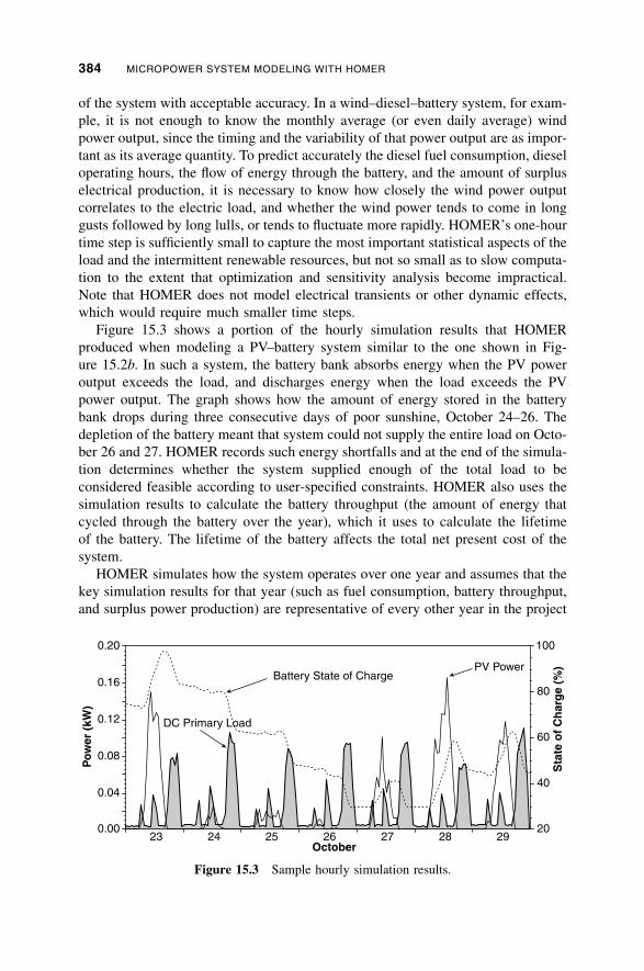
Figure 15.3 shows a portion of the hourly simulation results that HOMER

produced when modeling a PV–battery system similar to the one shown in Fig-

ure 15.2b. In such a system, the battery bank absorbs energy when the PV power

output exceeds the load, and discharges energy when the load exceeds the PV

power output. The graph shows how the amount of energy stored in the battery

bank drops during three consecutive days of poor sunshine, October 24–26. The

depletion of the battery meant that system could not supply the entire load on Octo-

ber 26 and 27. HOMER records such energy shortfalls and at the end of the simula-

tion determines whether the system supplied enough of the total load to be

considered feasible according to user-specified constraints. HOMER also uses the

simulation results to calculate the battery throughput (the amount of energy that

cycled through the battery over the year), which it uses to calculate the lifetime

of the battery. The lifetime of the battery affects the total net present cost of the

system.

HOMER simulates how the system operates over one year and assumes that the

key simulation results for that year (such as fuel consumption, battery throughput,

and surplus power production) are representative of every other year in the project

20

40

60

80

100

October23 24 25 26 27 28 29

0.00

0.04

0.08

0.12

0.16

0.20

Po

wer

(kW

)

Sta

te o

f C

har

ge

(%)

Battery State of Charge

DC Primary Load

PV Power

Figure 15.3 Sample hourly simulation results.


lifetime. It does not consider changes over time, such as load growth or the dete-

rioration of battery performance with aging. The modeler can, however, analyze

many of these effects using sensitivity analysis, described in Section 15.4. In Sec-

tions 15.5 and 15.6 we discuss in greater detail the technical and economic aspects

of HOMER’s simulation process.

15.3 OPTIMIZATION

Whereas the simulation process models a particular system configuration, the opti-

mization process determines the best possible system configuration. In HOMER,

the best possible, or optimal, system configuration is the one that satisfies the

user-specified constraints at the lowest total net present cost. Finding the optimal

system configuration may involve deciding on the mix of components that the

system should contain, the size or quantity of each component, and the dispatch

strategy the system should use. In the optimization process, HOMER simulates

many different system configurations, discards the infeasible ones (those that do

not satisfy the user-specified constraints), ranks the feasible ones according to total

net present cost, and presents the feasible one with the lowest total net present cost

as the optimal system configuration.

The goal of the optimization process is to determine the optimal value of each

decision variable that interests the modeler. A decision variable is a variable over

which the system designer has control and for which HOMER can consider multi-

ple possible values in its optimization process. Possible decision variables in

HOMER include:

� The size of the PV array

� The number of wind turbines

� The presence of the hydro system (HOMER can consider only one size of

hydro system; the decision is therefore whether or not the power system

should include the hydro system)

� The size of each generator

� The number of batteries

� The size of the ac–dc converter

� The size of the electrolyzer

� The size of the hydrogen storage tank

� The dispatch strategy (the set of rules governing how the system operates)

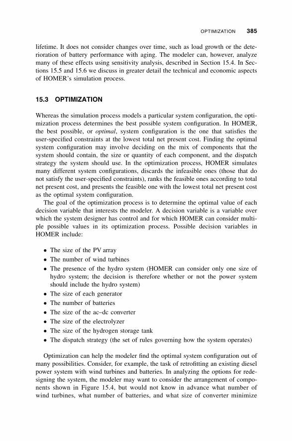
Optimization can help the modeler find the optimal system configuration out of

many possibilities. Consider, for example, the task of retrofitting an existing diesel

power system with wind turbines and batteries. In analyzing the options for rede-

signing the system, the modeler may want to consider the arrangement of compo-

nents shown in Figure 15.4, but would not know in advance what number of

wind turbines, what number of batteries, and what size of converter minimize

OPTIMIZATION 385

the life-cycle cost. These three variables would therefore be decision variables in

this analysis. The dispatch strategy could also be a decision variable, but for sim-

plicity this discussion will exclude the dispatch strategy. In Section 15.5.4 we dis-

cuss dispatch strategy in greater detail.

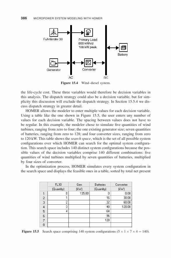
HOMER allows the modeler to enter multiple values for each decision variable.

Using a table like the one shown in Figure 15.5, the user enters any number of

values for each decision variable. The spacing between values does not have to

be regular. In this example, the modeler chose to simulate five quantities of wind

turbines, ranging from zero to four; the one existing generator size; seven quantities

of batteries, ranging from zero to 128; and four converter sizes, ranging from zero

to 120 kW. This table shows the search space, which is the set of all possible system

configurations over which HOMER can search for the optimal system configura-

tion. This search space includes 140 distinct system configurations because the pos-

sible values of the decision variables comprise 140 different combinations: five

quantities of wind turbines multiplied by seven quantities of batteries, multiplied

by four sizes of converter.

In the optimization process, HOMER simulates every system configuration in

the search space and displays the feasible ones in a table, sorted by total net present

Figure 15.4 Wind–diesel system.

Figure 15.5 Search space comprising 140 system configurations (5 � 1 � 7 � 4 ¼ 140).


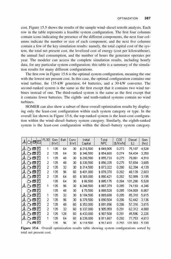
cost. Figure 15.5 shows the results of the sample wind–diesel retrofit analysis. Each

row in the table represents a feasible system configuration. The first four columns

contain icons indicating the presence of the different components, the next four col-

umns indicate the number or size of each component, and the next five columns

contain a few of the key simulation results: namely, the total capital cost of the sys-

tem, the total net present cost, the levelized cost of energy (cost per kilowatthour),

the annual fuel consumption, and the number of hours the generator operates per

year. The modeler can access the complete simulation results, including hourly

data, for any particular system configuration; this table is a summary of the simula-

tion results for many different configurations.

The first row in Figure 15.6 is the optimal system configuration, meaning the one

with the lowest net present cost. In this case, the optimal configuration contains one

wind turbine, the 135-kW generator, 64 batteries, and a 30-kW converter. The

second-ranked system is the same as the first except that it contains two wind tur-

bines instead of one. The third-ranked system is the same as the first except that

it contains fewer batteries. The eighth- and tenth-ranked systems contain no wind

turbines.

HOMER can also show a subset of these overall optimization results by display-

ing only the least-cost configuration within each system category or type. In the

overall list shown in Figure 15.6, the top-ranked system is the least-cost configura-

tion within the wind–diesel–battery system category. Similarly, the eighth-ranked

system is the least-cost configuration within the diesel–battery system category.

Figure 15.6 Overall optimization results table showing system configurations sorted by

total net present cost.

OPTIMIZATION 387

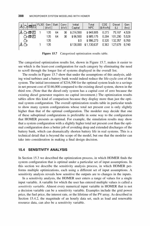
The categorized optimization results list, shown in Figure 15.7, makes it easier to

see which is the least-cost configuration for each category by eliminating the need

to scroll through the longer list of systems displayed in the overall list.

The results in Figure 15.7 show that under the assumptions of this analysis, add-

ing wind turbines and a battery bank would indeed reduce the life-cycle cost of the

system. The initial investment of $216,500 for the optimal system leads to a savings

in net present cost of $146,000 compared to the existing diesel system, shown in the

third row. (Note that the diesel-only system has a capital cost of zero because the

existing diesel generator requires no capital investment.) The optimization results

tables allow this kind of comparison because they display more than just the opti-

mal system configuration. The overall optimization results table in particular tends

to show many system configurations whose total net present cost is only slightly

higher than that of the optimal configuration. The modeler may decide that one

of these suboptimal configurations is preferable in some way to the configuration

that HOMER presents as optimal. For example, the simulation results may show

that a system configuration with a slightly higher total net present cost than the opti-

mal configuration does a better job of avoiding deep and extended discharges of the

battery bank, which can dramatically shorten battery life in real systems. This is a

technical detail that is beyond the scope of the model, but one that the modeler can

take into consideration in making a final design decision.

15.4 SENSITIVITY ANALYSIS

In Section 15.3 we described the optimization process, in which HOMER finds the

system configuration that is optimal under a particular set of input assumptions. In

this section we describe the sensitivity analysis process, in which HOMER per-

forms multiple optimizations, each using a different set of input assumptions. A

sensitivity analysis reveals how sensitive the outputs are to changes in the inputs.

In a sensitivity analysis, the HOMER user enters a range of values for a single

input variable. A variable for which the user has entered multiple values is called a

sensitivity variable. Almost every numerical input variable in HOMER that is not

a decision variable can be a sensitivity variable. Examples include the grid power

price, the fuel price, the interest rate, or the lifetime of the PV array. As described in

Section 15.4.2, the magnitude of an hourly data set, such as load and renewable

resource data, can also be a sensitivity variable.

Figure 15.7 Categorized optimization results table.


The HOMER user can perform a sensitivity analysis with any number of sensi-

tivity variables. Each combination of sensitivity variable values defines a distinct

sensitivity case. For example, if the user specifies six values for the grid power price

and four values for the interest rate, that defines 24 distinct sensitivity cases.

HOMER performs a separate optimization process for each sensitivity case and

presents the results in various tabular and graphic formats.

One of the primary uses of sensitivity analysis is in dealing with uncertainty. If a

system designer is unsure of the value of a particular variable, he or she can enter

several values covering the likely range and see how the results vary across that

range. But sensitivity analysis has applications beyond coping with uncertainty.

A system designer can use sensitivity analysis to evaluate trade-offs and answer

such questions as: How much additional capital investment is required to achieve

50% or 100% renewable energy production? An energy planner can determine

which technologies, or combinations of technologies, are optimal under different

conditions. A market analyst can determine at what price, or under what conditions,

a product (e.g., a fuel cell or a wind turbine) competes with the alternatives. A pol-

icy analyst can determine what level of incentive is needed to stimulate the market

for a particular technology, or what level of emissions penalty would tilt the eco-

nomics toward cleaner technologies.

15.4.1 Dealing with Uncertainty

A challenge that often confronts the micropower system designer is uncertainty in

key variables. Sensitivity analysis can help the designer understand the effects of

uncertainty and make good design decisions despite uncertainty. For example, con-

sider the wind–diesel system analysis in Section 15.3. In performing this analysis,

the modeler assumed that the price of diesel fuel would be $0.60 per liter over the

25-year project lifetime. There is obviously substantial uncertainty in this value, but

many other inputs may be uncertain as well, such as the lifetime of the wind tur-

bine, the maintenance cost of the diesel engine, the long-term average wind speed at

the site, and even the average electric load. Sensitivity analysis can help the mode-

ler to determine the effect that variations in these inputs have on the behavior, fea-

sibility, and economics of a particular system configuration; the robustness of a

particular system configuration (in other words, whether it is nearly optimal in

all scenarios, or far from optimal in certain scenarios); and how the optimal system

configuration changes across the range of uncertainty.

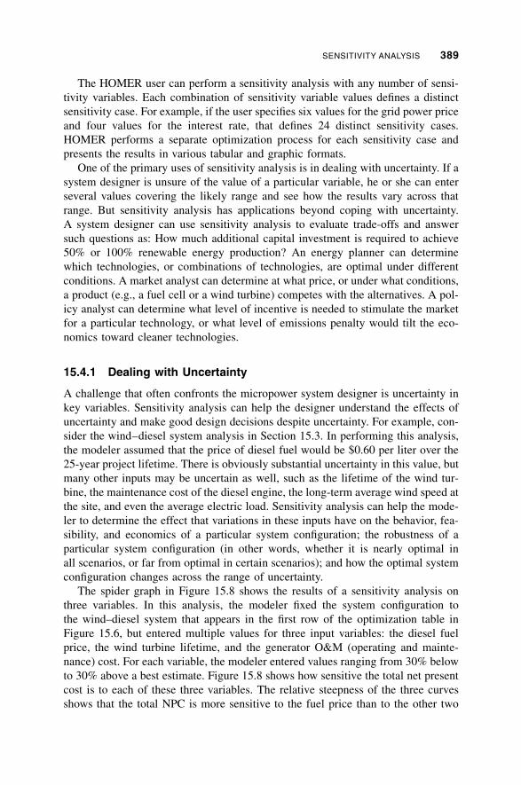
The spider graph in Figure 15.8 shows the results of a sensitivity analysis on

three variables. In this analysis, the modeler fixed the system configuration to

the wind–diesel system that appears in the first row of the optimization table in

Figure 15.6, but entered multiple values for three input variables: the diesel fuel

price, the wind turbine lifetime, and the generator O&M (operating and mainte-

nance) cost. For each variable, the modeler entered values ranging from 30% below

to 30% above a best estimate. Figure 15.8 shows how sensitive the total net present

cost is to each of these three variables. The relative steepness of the three curves

shows that the total NPC is more sensitive to the fuel price than to the other two

SENSITIVITY ANALYSIS 389

variables. Such information can help a system designer to establish the bounds of a

confidence interval or to prioritize efforts to reduce uncertainty.

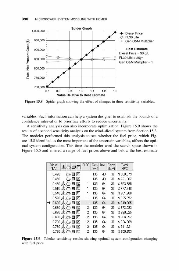
A sensitivity analysis can also incorporate optimization. Figure 15.9 shows the

results of a second sensitivity analysis on the wind–diesel system from Section 15.3.

The modeler performed this analysis to see whether the fuel price, which Fig-

ure 15.8 identified as the most important of the uncertain variables, affects the opti-

mal system configuration. This time the modeler used the search space shown in

Figure 15.5 and entered a range of fuel prices above and below the best-estimate

0.7 0.8 0.9 1.0 1.1 1.2 1.3700,000

750,000

800,000

850,000

900,000

950,000

1,000,000T

ota

l Net

Pre

sen

t C

ost

($)

Spider Graph

Value Relative to Best Estimate

Diesel PriceFL30 LifeGen O&M Multiplier

Best EstimateDiesel Price = $0.6/LFL30 Life = 25yrGen O&M Multiplier = 1

Figure 15.8 Spider graph showing the effect of changes in three sensitivity variables.

Figure 15.9 Tabular sensitivity results showing optimal system configuration changing

with fuel price.


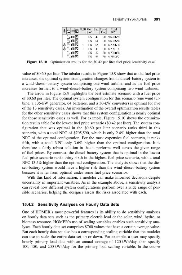
value of $0.60 per liter. The tabular results in Figure 15.9 show that as the fuel price

increases, the optimal system configuration changes from a diesel–battery system to

a wind–diesel–battery system comprising one wind turbine, and as the fuel price

increases further, to a wind–diesel–battery system comprising two wind turbines.

The arrow in Figure 15.9 highlights the best estimate scenario with a fuel price

of $0.60 per liter. The optimal system configuration for this scenario (one wind tur-

bine, a 135-kW generator, 64 batteries, and a 30-kW converter) is optimal for five

of the 13 sensitivity cases. An investigation of the overall optimization results tables

for the other sensitivity cases shows that this system configuration is nearly optimal

for those sensitivity cases as well. For example, Figure 15.10 shows the optimiza-

tion results table for the lowest fuel price scenario ($0.42 per liter). The system con-

figuration that was optimal in the $0.60 per liter scenario ranks third in this

scenario, with a total NPC of $705,590, which is only 2.4% higher than the total

NPC of the optimal configuration. For the most expensive fuel scenario, it ranks

fifth, with a total NPC only 3.6% higher than the optimal configuration. It is

therefore a fairly robust solution in that it performs well across the given range

of fuel prices. By contrast, the diesel–battery system that is optimal in the lowest

fuel price scenario ranks thirty-sixth in the highest fuel price scenario, with a total

NPC 13.5% higher than the optimal configuration. The analysis shows that the die-

sel–battery system would have a higher risk than the wind–diesel–battery system

because it is far from optimal under some fuel price scenarios.

With this kind of information, a modeler can make informed decisions despite

uncertainty in important variables. As in the example above, a sensitivity analysis

can reveal how different system configurations perform over a wide range of pos-

sible scenarios, helping the designer assess the risks associated with each.

15.4.2 Sensitivity Analyses on Hourly Data Sets

One of HOMER’s most powerful features is its ability to do sensitivity analyses

on hourly data sets such as the primary electric load or the solar, wind, hydro, or

biomass resource. HOMER’s use of scaling variables enables such sensitivity ana-

lyses. Each hourly data set comprises 8760 values that have a certain average value.

But each hourly data set also has a corresponding scaling variable that the modeler

can use to scale the entire data set up or down. For example, a user may specify

hourly primary load data with an annual average of 120 kWh/day, then specify

100, 150, and 200 kWh/day for the primary load scaling variable. In the course

Figure 15.10 Optimization results for the $0.42 per liter fuel price sensitivity case.

SENSITIVITY ANALYSIS 391

of the sensitivity analysis, HOMER will scale the load data so that it averages first

100 kWh/day, then 150 kWh/day, and finally, 200 kWh/day. This scaling process

changes the magnitude of the load data set without affecting the daily load shape,

the seasonal pattern, or any other statistical properties. HOMER scales renewable

resource data in the same manner.

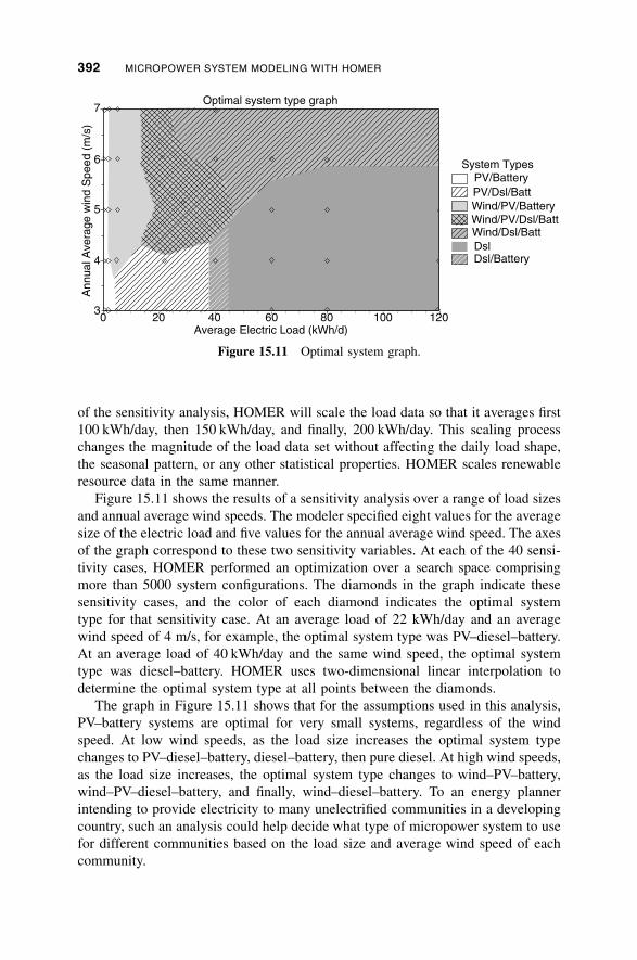
Figure 15.11 shows the results of a sensitivity analysis over a range of load sizes

and annual average wind speeds. The modeler specified eight values for the average

size of the electric load and five values for the annual average wind speed. The axes

of the graph correspond to these two sensitivity variables. At each of the 40 sensi-

tivity cases, HOMER performed an optimization over a search space comprising

more than 5000 system configurations. The diamonds in the graph indicate these

sensitivity cases, and the color of each diamond indicates the optimal system

type for that sensitivity case. At an average load of 22 kWh/day and an average

wind speed of 4 m/s, for example, the optimal system type was PV–diesel–battery.

At an average load of 40 kWh/day and the same wind speed, the optimal system

type was diesel–battery. HOMER uses two-dimensional linear interpolation to

determine the optimal system type at all points between the diamonds.

The graph in Figure 15.11 shows that for the assumptions used in this analysis,

PV–battery systems are optimal for very small systems, regardless of the wind

speed. At low wind speeds, as the load size increases the optimal system type

changes to PV–diesel–battery, diesel–battery, then pure diesel. At high wind speeds,

as the load size increases, the optimal system type changes to wind–PV–battery,

wind–PV–diesel–battery, and finally, wind–diesel–battery. To an energy planner

intending to provide electricity to many unelectrified communities in a developing

country, such an analysis could help decide what type of micropower system to use

for different communities based on the load size and average wind speed of each

community.

1201008060402003

4

5

6

7

Average Electric Load (kWh/d)

Ann

ual A

vera

ge w

ind

Spe

ed (

m/s

)Optimal system type graph

System TypesPV/BatteryPV/Dsl/BattWind/PV/BatteryWind/PV/Dsl/BattWind/Dsl/BattDslDsl/Battery

Figure 15.11 Optimal system graph.


15.5 PHYSICAL MODELING

In Section 15.2 we discussed the role of simulation and briefly described the pro-

cess HOMER uses to simulate micropower systems. In this section we provide

greater detail on how HOMER models the physical operation of a system. In

HOMER, a micropower system must comprise at least one source of electrical or

thermal energy (such as a wind turbine, a diesel generator, a boiler, or the grid), and

at least one destination for that energy (an electrical or thermal load, or the ability

to sell electricity to the grid). It may also comprise conversion devices such as an

ac–dc converter or an electrolyzer, and energy storage devices such as a battery

bank or a hydrogen storage tank.

In the following subsections we describe how HOMER models the loads that the

system must serve, the components of the system and their associated resources,

and how that collection of components operates together to serve the loads.

15.5.1 Loads

In HOMER, the term load refers to a demand for electric or thermal energy. Serving

loads is the reason for the existence of micropower systems, so the modeling of a

micropower system begins with the modeling of the load or loads that the system

must serve. HOMER models three types of loads. Primary load is electric demand

that must be served according to a particular schedule. Deferrable load is electric

demand that can be served at any time within a certain time span. Thermal load is

demand for heat.

Primary Load Primary load is electrical demand that the power system must

meet at a specific time. Electrical demand associated with lights, radio, TV, house-

hold appliances, computers, and industrial processes is typically modeled as pri-

mary load. When a consumer switches on a light, the power system must supply

electricity to that light immediately—the load cannot be deferred until later. If elec-

trical demand exceeds supply, there is a shortfall that HOMER records as unmet

load.

The HOMER user specifies an amount of primary load in kilowatts for each hour

of the year, either by importing a file containing hourly data or by allowing

HOMER to synthesize hourly data from average daily load profiles. When synthe-

sizing load data, HOMER creates hourly load values based on user-specified daily

load profiles. The modeler can specify a single 24-hour profile that applies through-

out the year, or can specify different profiles for different months and different pro-

files for weekdays and weekends. HOMER adds a user-specified amount of

randomness to synthesized load data so that every day’s load pattern is unique.

HOMER can model two separate primary loads, each of which can be ac or dc.

Among the three types of loads modeled in HOMER, primary load receives spe-

cial treatment in that it requires a user-specified amount of operating reserve. Oper-

ating reserve is surplus electrical generating capacity that is operating and can

respond instantly to a sudden increase in the electric load or a sudden decrease

PHYSICAL MODELING 393

in the renewable power output. Although it has the same meaning as the more com-

mon term spinning reserve, we call it operating reserve because batteries, fuel cells,

and the grid can provide it, but they do not spin. When simulating the operation of

the system, HOMER attempts to ensure that the system’s operating capacity is

always sufficient to supply the primary load and the required operating reserve.

Section 15.5.4 covers operating reserve in greater detail.

Deferrable Load Deferrable load is electrical demand that can be met anytime

within a defined time interval. Water pumps, ice makers, and battery-charging sta-

tions are examples of deferrable loads because the storage inherent to each of those

loads allows some flexibility as to when the system can serve them. The ability to

defer serving a load is often advantageous for systems comprising intermittent

renewable power sources, because it reduces the need for precise control of the tim-

ing of power production. If the renewable power supply ever exceeds the primary

load, the surplus can serve the deferrable load rather than going to waste.

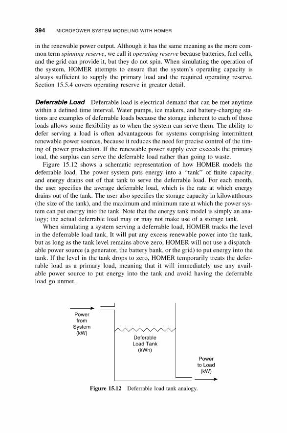
Figure 15.12 shows a schematic representation of how HOMER models the

deferrable load. The power system puts energy into a ‘‘tank’’ of finite capacity,

and energy drains out of that tank to serve the deferrable load. For each month,

the user specifies the average deferrable load, which is the rate at which energy

drains out of the tank. The user also specifies the storage capacity in kilowatthours

(the size of the tank), and the maximum and minimum rate at which the power sys-

tem can put energy into the tank. Note that the energy tank model is simply an ana-

logy; the actual deferrable load may or may not make use of a storage tank.

When simulating a system serving a deferrable load, HOMER tracks the level

in the deferrable load tank. It will put any excess renewable power into the tank,

but as long as the tank level remains above zero, HOMER will not use a dispatch-

able power source (a generator, the battery bank, or the grid) to put energy into the

tank. If the level in the tank drops to zero, HOMER temporarily treats the defer-

rable load as a primary load, meaning that it will immediately use any avail-

able power source to put energy into the tank and avoid having the deferrable

load go unmet.

DeferableLoad Tank

(kWh)

Powerto Load

(kW)

Powerfrom

System(kW)

Figure 15.12 Deferrable load tank analogy.


Thermal Load HOMER models thermal load in the same way that it models

primary electric load, except that the concept of operating reserve does not apply

to the thermal load. The user specifies the amount of thermal load for each hour of

the year, either by importing a file containing hourly data or by allowing HOMER

to synthesize hourly data from 24-hour load profiles. The system supplies the ther-

mal load with either the boiler, waste heat recovered from a generator, or resistive

heating using excess electricity.

15.5.2 Resources

The term resource applies to anything coming from outside the system that is used

by the system to generate electric or thermal power. That includes the four renew-

able resources (solar, wind, hydro, and biomass) as well as any fuel used by the

components of the system. Renewable resources vary enormously by location.

The solar resource depends strongly on latitude and climate, the wind resource

on large-scale atmospheric circulation patterns and geographic influences, the

hydro resource on local rainfall patterns and topography, and the biomass resource

on local biological productivity. Moreover, at any one location a renewable resource

may exhibit strong seasonal and hour-to-hour variability. The nature of the available

renewable resources affects the behavior and economics of renewable power sys-

tems, since the resource determines the quantity and the timing of renewable power

production. The careful modeling of the renewable resources is therefore an essen-

tial element of system modeling. In this section we describe how HOMER models

the four renewable resources and the fuel.

Solar Resource To model a system containing a PV array, the HOMER user

must provide solar resource data for the location of interest. Solar resource data indi-

cate the amount of global solar radiation (beam radiation coming directly from the

sun, plus diffuse radiation coming from all parts of the sky) that strikes Earth’s

surface in a typical year. The data can be in one of three forms: hourly average global

solar radiation on the horizontal surface (kW/m2), monthly average global solar

radiation on the horizontal surface (kWh/m2 �day), or monthly average clearness

index. The clearness index is the ratio of the solar radiation striking Earth’s surface

to the solar radiation striking the top of the atmosphere. A number between zero and

1, the clearness index is a measure of the clearness of the atmosphere.

If the user chooses to provide monthly solar resource data, HOMER generates

synthetic hourly global solar radiation data using an algorithm developed by

Graham and Hollands [7]. The inputs to this algorithm are the monthly average

solar radiation values and the latitude. The output is an 8760-hour data set with sta-

tistical characteristics similar to those of real measured data sets. One of those sta-

tistical properties is autocorrelation, which is the tendency for one day to be similar

to the preceding day, and for one hour to be similar to the preceding hour.

Wind Resource To model a system comprising one or more wind turbines,

the HOMER user must provide wind resource data indicating the wind speeds


the turbines would experience in a typical year. The user can provide measured

hourly wind speed data if available. Otherwise, HOMER can generate synthetic

hourly data from 12 monthly average wind speeds and four additional statistical

parameters: the Weibull shape factor, the autocorrelation factor, the diurnal pattern

strength, and the hour of peak wind speed. The Weibull shape factor is a measure of

the distribution of wind speeds over the year. The autocorrelation factor is a measure

of how strongly the wind speed in one hour tends to depend on the wind speed in the

preceding hour. The diurnal pattern strength and the hour of peak wind speed indi-

cate the magnitude and the phase, respectively, of the average daily pattern in the

wind speed. HOMER provides default values for each of these parameters.

The user indicates the anemometer height, meaning the height above ground at

which the wind speed data were measured or for which they were estimated. If the

wind turbine hub height is different from the anemometer height, HOMER calcu-

lates the wind speed at the turbine hub height using either the logarithmic law,

which assumes that the wind speed is proportional to the logarithm of the height

above ground, or the power law, which assumes that the wind speed varies expo-

nentially with height. To use the logarithmic law, the user enters the surface rough-

ness length, which is a parameter characterizing the roughness of the surrounding

terrain. To use the power law, the user enters the power law exponent.

The user also indicates the elevation of the site above sea level, which HOMER

uses to calculate the air density according to the U.S. Standard Atmosphere,

described in Section 2.3 of White [6]. HOMER makes use of the air density

when calculating the output of the wind turbine, as described in Section 15.5.3.

Hydro Resource To model a system comprising a run-of-river hydro turbine,

the HOMER user must provide stream flow data indicating the amount of water

available to the turbine in a typical year. The user can provide measured hourly

stream flow data if available. Otherwise, HOMER can use monthly averages under

the assumption that the flow rate remains constant within each month. The user also

specifies the residual flow, which is the minimum stream flow that must bypass the

hydro turbine for ecological purposes. HOMER subtracts the residual flow from the

stream flow data to determine the stream flow available to the turbine.

Biomass Resource The biomass resource takes various forms (e.g., wood

waste, agricultural residue, animal waste, energy crops) and may be used to produce

heat or electricity. HOMER models biomass power systems that convert biomass

into electricity. Two aspects of the biomass resource make it unique among the

four renewable resources that HOMER models. First, the availability of the

resource depends in part on human effort for harvesting, transportation, and storage.

It is consequently not intermittent, although it may be seasonal. It is also often not

free. Second, the biomass feedstock may be converted to a gaseous or liquid fuel, to

be consumed in an otherwise conventional generator. The modeling of the biomass

resource is therefore similar in many ways to the modeling of any other fuel.

The HOMER user can model the biomass resource in two ways. The simplest

way is to define a fuel with properties corresponding to the biomass feedstock


and then specify the fuel consumption of the generator to show electricity produced

versus biomass feedstock consumed. This approach implicitly, rather than expli-

citly, models the process of converting the feedstock into a fuel suitable for the gen-

erator, if such a process occurs. The second alternative is to use HOMER’s biomass

resource inputs, which allow the modeler to specify the availability of the feedstock

throughout the year, and to model explicitly the feedstock conversion process. In

the remainder of this section we focus on this second alternative. In the next section

we address the fuel inputs.

As with the other renewable resource data sets, the HOMER user can indicate

the availability of biomass feedstock by importing an hourly data file or using

monthly averages. If the user specifies monthly averages, HOMER assumes that

the availability remains constant within each month.

The user must specify four additional parameters to define the biomass resource:

price, carbon content, gasification ratio, and the energy content of the biomass fuel.

For greenhouse gas analyses, the carbon content value should reflect the net amount

of carbon released to the atmosphere by the harvesting, processing, and consump-

tion of the biomass feedstock, considering the fact that the carbon in the feedstock

was originally in the atmosphere. The gasification ratio, despite its name, applies

equally well to liquid and gaseous fuels. It is the fuel conversion ratio, indicating

the ratio of the mass of generator-ready fuel emerging from the fuel conversion pro-

cess to the mass of biomass feedstock entering the fuel conversion process.

HOMER uses the energy content of the biomass fuel to calculate the thermody-

namic efficiency of the generator that consumes the fuel.

Fuel HOMER provides a library of several predefined fuels, and users can add to

the library if necessary. The physical properties of a fuel include its density, lower

heating value, carbon content, and sulfur content. The user can also choose the most

appropriate measurement units, either L, m3, or kg. The two remaining properties of

the fuel are the price and the annual consumption limit, if any.

15.5.3 Components

In HOMER, a component is any part of a micropower system that generates, deli-

vers, converts, or stores energy. HOMER models 10 types of components. Three

generate electricity from intermittent renewable sources: photovoltaic modules,

wind turbines, and hydro turbines. PV modules convert solar radiation into dc elec-

tricity. Wind turbines convert wind energy into ac or dc electricity. Hydro turbines

convert the energy of flowing water into ac or dc electricity. HOMER can only

model run-of-river hydro installations, meaning those that do not comprise a sto-

rage reservoir.

Another three types of components, generators, the grid, and boilers, are dis-

patchable energy sources, meaning that the system can control them as needed.

Generators consume fuel to produce ac or dc electricity. A generator may also pro-

duce thermal power via waste heat recovery. The grid delivers ac electricity to a


grid-connected system and may also accept surplus electricity from the system.

Boilers consume fuel to produce thermal power.

Two types of components, converters and electrolyzers, convert electrical energy

into another form. Converters convert electricity from ac to dc or from dc to ac.

Electrolyzers convert surplus ac or dc electricity into hydrogen via the electrolysis

of water. The system can store the hydrogen and use it as fuel for one or more gen-

erators. Finally, two types of components store energy: batteries and hydrogen sto-

rage tanks. Batteries store dc electricity. Hydrogen tanks store hydrogen from the

electrolyzer to fuel one or more generators.

In this section we explain how HOMER models each of these components

and discuss the physical and economic properties that the user can use to describe

each.

PV Array HOMER models the PV array as a device that produces dc electricity

in direct proportion to the global solar radiation incident upon it, independent of its

temperature and the voltage to which it is exposed. HOMER calculates the power

output of the PV array using the equation

PPV ¼ fPVYPV

IT

IS

ð15:1Þ

Where, fPV is the PV derating factor,YPV the rated capacity of the PV array (kW),

IT the global solar radiation (beam plus diffuse) incident on the surface of the PV

array (kW/m2), and IS is 1 kW/m2, which is the standard amount of radiation used

to rate the capacity of the PV array. In the following paragraphs we describe these

variables in more detail.

The rated capacity (sometimes called the peak capacity) of a PV array is the

amount of power it would produce under standard test conditions of 1 kW/m2 irra-

diance and a panel temperature of 25�C. In HOMER, the size of a PV array is

always specified in terms of rated capacity. The rated capacity accounts for both

the area and the efficiency of the PV module, so neither of those parameters appears

explicitly in HOMER. A 40-W module made of amorphous silicon (which has a

relatively low efficiency) will be larger than a 40-W module made of polycrystal-

line silicon (which has a relatively high efficiency), but that size difference is of no

consequence to HOMER.

Each hour of the year, HOMER calculates the global solar radiation incident

on the PV array using the HDKR model, explained in Section 2.16 of Duffie and

Beckmann [5]. This model takes into account the current value of the solar resource

(the global solar radiation incident on a horizontal surface), the orientation of the

PV array, the location on Earth’s surface, the time of year, and the time of day.

The orientation of the array may be fixed or may vary according to one of several

tracking schemes.

The derating factor is a scaling factor meant to account for effects of dust on the

panel, wire losses, elevated temperature, or anything else that would cause the out-

put of the PV array to deviate from that expected under ideal conditions. HOMER

does not account for the fact that the power output of a PV array decreases with


increasing panel temperature, but the HOMER user can reduce the derating factor

to (crudely) correct for this effect when modeling systems for hot climates.

In reality, the output of a PV array does depend strongly and nonlinearly on the

voltage to which it is exposed. The maximum power point (the voltage at which the

power output is maximized) depends on the solar radiation and the temperature. If

the PV array is connected directly to a dc load or a battery bank, it will often be

exposed to a voltage different from the maximum power point, and performance

will suffer. A maximum power point tracker (MPPT) is a solid-state device placed

between the PV array and the rest of the dc components of the system that decou-

ples the array voltage from that of the rest of the system, and ensures that the array

voltage is always equal to the maximum power point. By ignoring the effect of

the voltage to which the PV array is exposed, HOMER effectively assumes that a

maximum power point tracker is present in the system.

To describe the cost of the PV array, the user specifies its initial capital cost in

dollars, replacement cost in dollars, and operating and maintenance (O&M) cost in

dollars per year. The replacement cost is the cost of replacing the PV array at the

end of its useful lifetime, which the user specifies in years. By default, the replace-

ment cost is equal to the capital cost, but the two can differ for several reasons. For

example, a donor organization may cover some or all of the initial capital cost but

none of the replacement cost.

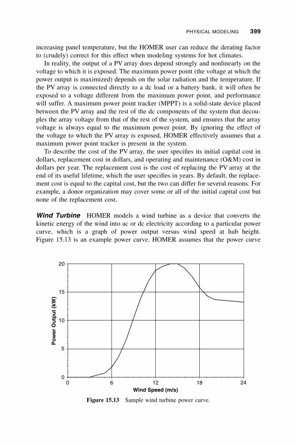
Wind Turbine HOMER models a wind turbine as a device that converts the

kinetic energy of the wind into ac or dc electricity according to a particular power

curve, which is a graph of power output versus wind speed at hub height.

Figure 15.13 is an example power curve. HOMER assumes that the power curve

0 12 18 240

5

10

15

20

Po

wer

Ou

tpu

t (k

W)

Wind Speed (m/s)6

Figure 15.13 Sample wind turbine power curve.


applies at a standard air density of 1.225 kg/m3, which corresponds to standard

temperature and pressure conditions.

Each hour, HOMER calculates the power output of the wind turbine in a

four-step process. First, it determines the average wind speed for the hour at the

anemometer height by referring to the wind resource data. Second, it calculates

the corresponding wind speed at the turbine’s hub height using either the logarith-

mic law or the power law. Third, it refers to the turbine’s power curve to calculate

its power output at that wind speed assuming standard air density. Fourth, it

multiplies that power output value by the air density ratio, which is the ratio of

the actual air density to the standard air density. As mentioned in Section 15.5.2,

HOMER calculates the air density ratio at the site elevation using the U.S. Standard

Atmosphere [6]. HOMER assumes that the air density ratio is constant throughout

the year.

In addition to the turbine’s power curve and hub height, the user specifies the

expected lifetime of the turbine in years, its initial capital cost in dollars, its repla-

cement cost in dollars, and its annual O&M cost in dollars per year.

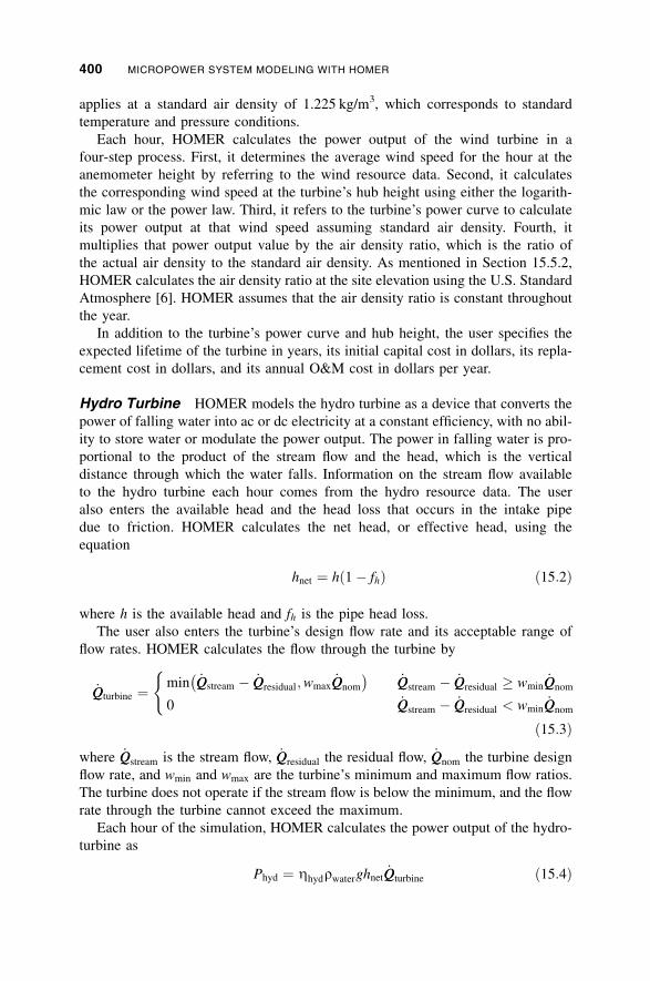
Hydro Turbine HOMER models the hydro turbine as a device that converts the

power of falling water into ac or dc electricity at a constant efficiency, with no abil-

ity to store water or modulate the power output. The power in falling water is pro-

portional to the product of the stream flow and the head, which is the vertical

distance through which the water falls. Information on the stream flow available

to the hydro turbine each hour comes from the hydro resource data. The user

also enters the available head and the head loss that occurs in the intake pipe

due to friction. HOMER calculates the net head, or effective head, using the

equation

hnet ¼ h 1 � fhð Þ ð15:2Þ

where h is the available head and fh is the pipe head loss.

The user also enters the turbine’s design flow rate and its acceptable range of

flow rates. HOMER calculates the flow through the turbine by

_QQturbine ¼min _QQstream � _QQresidual;wmax

_QQnom

� �_QQstream � _QQresidual wmin

_QQnom

0 _QQstream � _QQresidual < wmin_QQnom

(

ð15:3Þ

where _QQstream is the stream flow, _QQresidual the residual flow, _QQnom the turbine design

flow rate, and wmin and wmax are the turbine’s minimum and maximum flow ratios.

The turbine does not operate if the stream flow is below the minimum, and the flow

rate through the turbine cannot exceed the maximum.

Each hour of the simulation, HOMER calculates the power output of the hydro-

turbine as

Phyd ¼ Zhydrwaterghnet_QQturbine ð15:4Þ


where Zhyd is the turbine efficiency, rwater the density of water, g the gravitational

acceleration, hnet the net head, and _QQturbine the flow rate through the turbine. The

user specifies the expected lifetime of the hydro-turbine in years, as well as its

initial capital cost in dollars, replacement cost in dollars, and annual O&M cost

in dollars per year.

Generators A generator consumes fuel to produce electricity, and possibly heat

as a by-product. HOMER’s generator module is flexible enough to model a wide

variety of generators, including internal combustion engine generators, microtur-

bines, fuel cells, Stirling engines, thermophotovoltaic generators, and thermoelec-

tric generators. HOMER can model a power system comprising as many as three

generators, each of which can be ac or dc, and each of which can consume a

different fuel.

The principal physical properties of the generator are its maximum and mini-

mum electrical power output, its expected lifetime in operating hours, the type of

fuel it consumes, and its fuel curve, which relates the quantity of fuel consumed to

the electrical power produced. In HOMER, a generator can consume any of the

fuels listed in the fuel library (to which users can add their own fuels) or one of

two special fuels: electrolyzed hydrogen from the hydrogen storage tank, or bio-

mass derived from the biomass resource. It is also possible to cofire a generator

with a mixture of biomass and another fuel.

HOMER assumes the fuel curve is a straight line with a y-intercept and uses the

following equation for the generator’s fuel consumption:

F ¼ F0Ygen þ F1Pgen ð15:5Þ

where F0 is the fuel curve intercept coefficient, F1 is the fuel curve slope, Ygen the

rated capacity of the generator (kW), and Pgen the electrical output of the generator

(kW). The units of F depend on the measurement units of the fuel. If the fuel is

denominated in liters, the units of F are L/h. If the fuel is denominated in m3 or

kg, the units of F are m3/h or kg/h, respectively. In the same way, the units of F0

and F1 depend on the measurement units of the fuel. For fuels denominated in liters,

the units of F0 and F1 are L/h �kW.

For a generator that provides heat as well as electricity, the user also specifies the

heat recovery ratio. HOMER assumes that the generator converts all the fuel energy

into either electricity or waste heat. The heat recovery ratio is the fraction of that

waste heat that can be captured to serve the thermal load. In addition to these prop-

erties, the modeler can specify the generator emissions coefficients, which specify

the generator’s emissions of six different pollutants in grams of pollutant emitted

per quantity of fuel consumed.

The user can schedule the operation of the generator to force it on or off at cer-

tain times. During times that the generator is neither forced on or off, HOMER

decides whether it should operate based on the needs of the system and the relative

costs of the other power sources. During times that the generator is forced on,

HOMER decides at what power output level it operates, which may be anywhere

between its minimum and maximum power output.


The user specifies the generator’s initial capital cost in dollars, replacement cost

in dollars, and annual O&M cost in dollars per operating hour. The generator O&M

cost should account for oil changes and other maintenance costs, but not fuel cost

because HOMER calculates fuel cost separately. As it does for all dispatchable

power sources, HOMER calculates the generator’s fixed and marginal cost of

energy and uses that information when simulating the operation of the system.

The fixed cost of energy is the cost per hour of simply running the generator, with-

out producing any electricity. The marginal cost of energy is the additional cost per

kilowatthour of producing electricity from that generator.

HOMER uses the following equation to calculate the generator’s fixed cost of

energy:

cgen;fixed ¼ com;gen þCrep;gen

Rgen

þ F0Ygencfuel;eff ð15:6Þ

where com;gen is the O&M cost in dollars per hour, Crep;gen the replacement cost in

dollars, Rgen the generator lifetime in hours, F0 the fuel curve intercept coefficient

in quantity of fuel per hour per kilowatt, Ygen the capacity of the generator (kW),

and cfuel;eff the effective price of fuel in dollars per quantity of fuel. The effective

price of fuel includes the cost penalties, if any, associated with the emissions of

pollutants from the generator.

HOMER calculates the marginal cost of energy of the generator using the fol-

lowing equation:

cgen;mar ¼ F1cfuel;eff ð15:7Þ

where F1 is the fuel curve slope in quantity of fuel per hour per kilowatthour and

cfuel;eff is the effective price of fuel (including the cost of any penalties on emis-

sions) in dollars per quantity of fuel.

Battery Bank The battery bank is a collection of one or more individual bat-

teries. HOMER models a single battery as a device capable of storing a certain

amount of dc electricity at a fixed round-trip energy efficiency, with limits as to

how quickly it can be charged or discharged, how deeply it can be discharged with-

out causing damage, and how much energy can cycle through it before it needs

replacement. HOMER assumes that the properties of the batteries remain constant

throughout its lifetime and are not affected by external factors such as temperature.

In HOMER, the key physical properties of the battery are its nominal voltage,

capacity curve, lifetime curve, minimum state of charge, and round-trip efficiency.

The capacity curve shows the discharge capacity of the battery in ampere-hours ver-

sus the discharge current in amperes. Manufacturers determine each point on this

curve by measuring the ampere-hours that can be discharged at a constant current

out of a fully charged battery. Capacity typically decreases with increasing dis-

charge current. The lifetime curve shows the number of discharge–charge cycles

the battery can withstand versus the cycle depth. The number of cycles to failure

typically decreases with increasing cycle depth. The minimum state of charge is the


state of charge below which the battery must not be discharged to avoid permanent

damage. In the system simulation, HOMER does not allow the battery to be dis-

charged any deeper than this limit. The round-trip efficiency indicates the percen-

tage of the energy going into the battery that can be drawn back out.

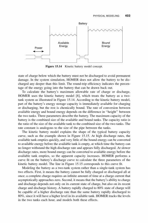
To calculate the battery’s maximum allowable rate of charge or discharge,

HOMER uses the kinetic battery model [8], which treats the battery as a two-

tank system as illustrated in Figure 15.14. According to the kinetic battery model,

part of the battery’s energy storage capacity is immediately available for charging

or discharging, but the rest is chemically bound. The rate of conversion between

available energy and bound energy depends on the difference in ‘‘height’’ between

the two tanks. Three parameters describe the battery. The maximum capacity of the

battery is the combined size of the available and bound tanks. The capacity ratio is

the ratio of the size of the available tank to the combined size of the two tanks. The

rate constant is analogous to the size of the pipe between the tanks.

The kinetic battery model explains the shape of the typical battery capacity

curve, such as the example shown in Figure 15.15. At high discharge rates, the

available tank empties quickly, and very little of the bound energy can be converted

to available energy before the available tank is empty, at which time the battery can

no longer withstand the high discharge rate and appears fully discharged. At slower

discharge rates, more bound energy can be converted to available energy before the

available tank empties, so the apparent capacity increases. HOMER performs a

curve fit on the battery’s discharge curve to calculate the three parameters of the

kinetic battery model. The line in Figure 15.15 corresponds to this curve fit.

Modeling the battery as a two-tank system rather than a single-tank system has

two effects. First, it means the battery cannot be fully charged or discharged all at

once; a complete charge requires an infinite amount of time at a charge current that

asymptotically approaches zero. Second, it means that the battery’s ability to charge

and discharge depends not only on its current state of charge, but also on its recent

charge and discharge history. A battery rapidly charged to 80% state of charge will

be capable of a higher discharge rate than the same battery rapidly discharged to

80%, since it will have a higher level in its available tank. HOMER tracks the levels

in the two tanks each hour, and models both these effects.

AvailableEnergy

BoundEnergy

Power

Battery

Figure 15.14 Kinetic battery model concept.


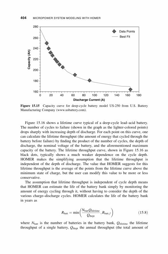
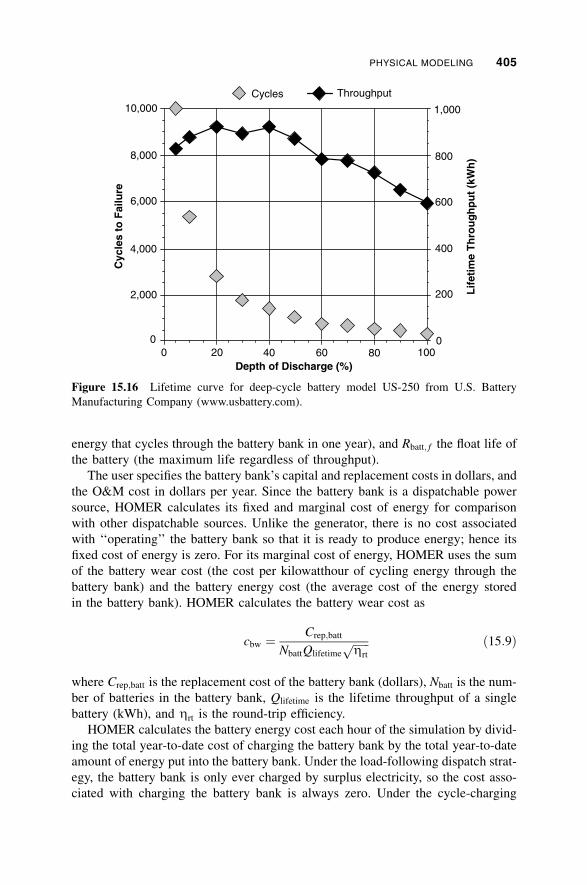
Figure 15.16 shows a lifetime curve typical of a deep-cycle lead–acid battery.

The number of cycles to failure (shown in the graph as the lighter-colored points)

drops sharply with increasing depth of discharge. For each point on this curve, one

can calculate the lifetime throughput (the amount of energy that cycled through the

battery before failure) by finding the product of the number of cycles, the depth of

discharge, the nominal voltage of the battery, and the aforementioned maximum

capacity of the battery. The lifetime throughput curve, shown in Figure 15.16 as

black dots, typically shows a much weaker dependence on the cycle depth.

HOMER makes the simplifying assumption that the lifetime throughput is

independent of the depth of discharge. The value that HOMER suggests for this

lifetime throughput is the average of the points from the lifetime curve above the

minimum state of charge, but the user can modify this value to be more or less

conservative.

The assumption that lifetime throughput is independent of cycle depth means

that HOMER can estimate the life of the battery bank simply by monitoring the

amount of energy cycling through it, without having to consider the depth of the

various charge–discharge cycles. HOMER calculates the life of the battery bank

in years as

Rbatt ¼ minNbattQlifetime

Qthrpt

;Rbatt; f

� �ð15:8Þ

where Nbatt is the number of batteries in the battery bank, Qlifetime the lifetime

throughput of a single battery, Qthrpt the annual throughput (the total amount of

0 20 40 60 80 100 120 140 160 180160

180

200

220

240

260

280C

apac

ity

(Ah

)

Discharge Current (A)

Data Points

Best Fit

Figure 15.15 Capacity curve for deep-cycle battery model US-250 from U.S. Battery

Manufacturing Company (www.usbattery.com).


energy that cycles through the battery bank in one year), and Rbatt; f the float life of

the battery (the maximum life regardless of throughput).

The user specifies the battery bank’s capital and replacement costs in dollars, and

the O&M cost in dollars per year. Since the battery bank is a dispatchable power

source, HOMER calculates its fixed and marginal cost of energy for comparison

with other dispatchable sources. Unlike the generator, there is no cost associated

with ‘‘operating’’ the battery bank so that it is ready to produce energy; hence its

fixed cost of energy is zero. For its marginal cost of energy, HOMER uses the sum

of the battery wear cost (the cost per kilowatthour of cycling energy through the

battery bank) and the battery energy cost (the average cost of the energy stored

in the battery bank). HOMER calculates the battery wear cost as

cbw ¼ Crep;batt

NbattQlifetimeffiffiffiffiffiffiZrt

p ð15:9Þ

where Crep;batt is the replacement cost of the battery bank (dollars), Nbatt is the num-

ber of batteries in the battery bank, Qlifetime is the lifetime throughput of a single

battery (kWh), and Zrt is the round-trip efficiency.

HOMER calculates the battery energy cost each hour of the simulation by divid-

ing the total year-to-date cost of charging the battery bank by the total year-to-date

amount of energy put into the battery bank. Under the load-following dispatch strat-

egy, the battery bank is only ever charged by surplus electricity, so the cost asso-

ciated with charging the battery bank is always zero. Under the cycle-charging

0

200

400

600

800

1,000

0 20 40 60 80 1000

2,000

4,000

6,000

8,000

10,000C

ycle

s to

Fai

lure

Depth of Discharge (%)

Lif

etim

e T

hro

ug

hp

ut

(kW

h)

Cycles Throughput

Figure 15.16 Lifetime curve for deep-cycle battery model US-250 from U.S. Battery

Manufacturing Company (www.usbattery.com).


strategy, however, a generator will produce extra electricity (and hence consume

additional fuel) for the express purpose of charging the battery bank, so the cost

associated with charging the battery bank is not zero. In Section 15.5.4 we discuss

dispatch strategies in greater detail.

Grid HOMER models the grid as a component from which the micropower sys-

tem can purchase ac electricity and to which the system can sell ac electricity. The

cost of purchasing power from the grid can comprise an energy charge based on the

amount of energy purchased in a billing period and a demand charge based on the

peak demand within the billing period. HOMER uses the term grid power price for

the price (in dollars per kilowatthour) that the electric utility charges for energy

purchased from the grid, and the demand rate for the price (in dollars per kilowatt

per month) the utility charges for the peak grid demand. A third term, the sellback

rate, refers to the price (in dollars per kilowatthour) that the utility pays for power

sold to the grid.

The HOMER user can define and schedule up to 16 different rates, each of which

can have different values of grid power price, demand rate, and sellback rate. The

schedule of the rates can vary according to month, time of day, and weekday/

weekend. For example, HOMER could model a situation where an expensive

rate applies during weekday afternoons in July and August, an intermediate rate

applies during weekday afternoons in June and September and weekend afternoons

from June to September, and an inexpensive rate applies at all other times.

HOMER can also model net metering, a billing arrangement whereby the utility

charges the customer based on the net grid purchases (purchases minus sales) over

the billing period. Under net metering, if purchases exceed sales over the billing

period, the consumer pays the utility an amount equal to the net grid purchases

times the grid power cost. If sales exceed purchases over the billing period, the uti-

lity pays the consumer an amount equal to the net grid sales (sales minus purchases)

times the sellback rate, which is typically less than the grid power price, and often

zero. The billing period may be one month or one year. In the unusual situation

where net metering applies to multiple rates, HOMER tracks the net grid purchases

separately for each rate.

Two variables describe the grid’s capacity to deliver and accept power. The

maximum power sale is the maximum rate at which the power system can sell power

to the grid. The user should set this value to zero if the utility does not allow sell-

back. The maximum grid demand is the maximum amount of power that can be

drawn from the grid. It is a decision variable because of the effect of demand

charges. HOMER does not explicitly consider the demand rate in its hour-by-hour

decisions as to how to control the power system; it simply calculates the demand

charge at the end of each simulation. As a result, when modeling a grid-connected

generator, HOMER will not turn on the generator simply to save demand charges.

But it will turn on a generator whenever the load exceeds the maximum grid

demand. The maximum grid demand therefore acts as a control parameter that

affects the operation and economics of the system. Because it is a decision variable,

the user can enter multiple values and HOMER can find the optimal one.


The user also enters the grid emissions coefficients, which HOMER uses to cal-

culate the emissions of six pollutants associated with buying power from the grid,

as well as the avoided emissions resulting from the sale of power to the grid. Each

emissions coefficient has units of grams of pollutant emitted per kilowatthour

consumed.

Because it is a dispatchable power source, HOMER calculates the grid’s fixed

and marginal cost of energy. The fixed cost is zero, and the marginal cost is equal

to the current grid power price plus any cost resulting from emissions penalties.

Since the grid power price can change from hour to hour as the applicable rate

changes, the grid’s marginal cost of energy can also change from hour to hour.

This can have important effects on HOMER’s simulation of the system’s behavior.

For example, HOMER may choose to run a generator only during times of high

grid power price, when the cost of grid power exceeds the cost of generator power.

Boiler HOMER models the boiler as an idealized component able to provide

an unlimited amount of thermal energy on demand. When dispatching generators

to serve the electric load, HOMER considers the value of any waste heat that

can be recovered from a generator to serve the thermal load, but it will not dispatch

a generator simply to serve the thermal load. It assumes that the system can always

rely on the boiler to serve any thermal load that the generators do not. To avoid

situations that violate this assumption, HOMER ensures that a boiler exists in

any system serving a thermal load, it does not allow any consumption limit on

the boiler fuel, and it does not allow the boiler to consume biomass or stored hydro-

gen (since either of those fuels could be unavailable at times).

The idealized nature of HOMER’s boiler model means that the user must specify

only a few physical properties of the boiler. The user selects the type of fuel the

boiler consumes and enters the efficiency with which it converts that fuel into

heat. The only other properties of the boiler are its emissions coefficients, which

are in units of grams of pollutant emitted per quantity of fuel consumed.

As it does for all dispatchable energy sources, HOMER calculates the fixed and

marginal cost of energy from the boiler. The fixed cost is zero. HOMER calculates

the marginal cost using the equation

cboiler;mar ¼3:6cfuel;eff

ZboilerLHVfuel

ð15:10Þ

where cfuel;eff is the effective price of the fuel (including the cost of any penalties on

emissions) in dollars per kilogram, Zboiler is the boiler efficiency, and LHVfuel is the

lower heating value of the fuel in MJ/kg.

Converter A converter is a device that converts electric power from dc to ac in a

process called inversion, and/or from ac to dc in a process called rectification.

HOMER can model the two common types of converters: solid-state and rotary.

The converter size, which is a decision variable, refers to the inverter capacity,

meaning the maximum amount of ac power that the device can produce by inverting


dc power. The user specifies the rectifier capacity, which is the maximum amount of

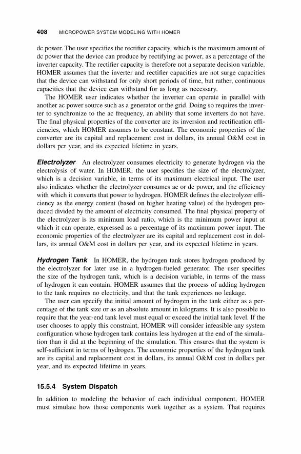
dc power that the device can produce by rectifying ac power, as a percentage of the

inverter capacity. The rectifier capacity is therefore not a separate decision variable.

HOMER assumes that the inverter and rectifier capacities are not surge capacities

that the device can withstand for only short periods of time, but rather, continuous

capacities that the device can withstand for as long as necessary.

The HOMER user indicates whether the inverter can operate in parallel with

another ac power source such as a generator or the grid. Doing so requires the inver-

ter to synchronize to the ac frequency, an ability that some inverters do not have.

The final physical properties of the converter are its inversion and rectification effi-

ciencies, which HOMER assumes to be constant. The economic properties of the

converter are its capital and replacement cost in dollars, its annual O&M cost in

dollars per year, and its expected lifetime in years.

Electrolyzer An electrolyzer consumes electricity to generate hydrogen via the

electrolysis of water. In HOMER, the user specifies the size of the electrolyzer,

which is a decision variable, in terms of its maximum electrical input. The user

also indicates whether the electrolyzer consumes ac or dc power, and the efficiency

with which it converts that power to hydrogen. HOMER defines the electrolyzer effi-

ciency as the energy content (based on higher heating value) of the hydrogen pro-

duced divided by the amount of electricity consumed. The final physical property of

the electrolyzer is its minimum load ratio, which is the minimum power input at

which it can operate, expressed as a percentage of its maximum power input. The

economic properties of the electrolyzer are its capital and replacement cost in dol-

lars, its annual O&M cost in dollars per year, and its expected lifetime in years.

Hydrogen Tank In HOMER, the hydrogen tank stores hydrogen produced by

the electrolyzer for later use in a hydrogen-fueled generator. The user specifies

the size of the hydrogen tank, which is a decision variable, in terms of the mass

of hydrogen it can contain. HOMER assumes that the process of adding hydrogen

to the tank requires no electricity, and that the tank experiences no leakage.

The user can specify the initial amount of hydrogen in the tank either as a per-

centage of the tank size or as an absolute amount in kilograms. It is also possible to

require that the year-end tank level must equal or exceed the initial tank level. If the

user chooses to apply this constraint, HOMER will consider infeasible any system

configuration whose hydrogen tank contains less hydrogen at the end of the simula-

tion than it did at the beginning of the simulation. This ensures that the system is

self-sufficient in terms of hydrogen. The economic properties of the hydrogen tank

are its capital and replacement cost in dollars, its annual O&M cost in dollars per

year, and its expected lifetime in years.

15.5.4 System Dispatch

In addition to modeling the behavior of each individual component, HOMER

must simulate how those components work together as a system. That requires


hour-by-hour decisions as to which generators should operate and at what power

level, whether to charge or discharge the batteries, and whether to buy from or

sell to the grid. In this section we describe briefly the logic HOMER uses to

make such decisions. A discussion of operating reserve comes first because the con-

cept of operating reserve significantly affects HOMER’s dispatch decisions.

Operating Reserve Operating reserve provides a safety margin that helps

ensure reliable electricity supply despite variability in the electric load and the

renewable power supply. Virtually every real micropower system must always pro-

vide some amount of operating reserve, because otherwise the electric load would

sometimes fluctuate above the operating capacity of the system, and an outage

would result.

At any given moment, the amount of operating reserve that a power system pro-

vides is equal to the operating capacity minus the electrical load. Consider, for

example, a simple diesel system in which an 80-kW diesel generator supplies an

electric load. In that system, if the load is 55 kW, the diesel will produce 55 kW

of electricity and provide 25 kW of operating reserve. In other words, the system

could supply the load even if the load suddenly increased by 25 kW. In HOMER,

the modeler specifies the required amount of operating reserve, and HOMER simu-

lates the system so as to provide at least that much operating reserve.

Each hour, HOMER calculates the required amount of operating reserve as a

fraction of the primary load that hour, plus a fraction of the annual peak primary

load, plus a fraction of the PV power output that hour, plus a fraction of the

wind power output that hour. The modeler specifies these fractions by considering

how much the load or the renewable power output is likely to fluctuate in a short

period, and how conservatively he or she plans to operate the system. The more vari-

able the load and renewable power output, and the more conservatively the system

must operate, the higher the fractions the modeler should specify. HOMER does not

attempt to ascertain the amount of operating reserve required to achieve different

levels of reliability; it simply uses the modeler’s specifications to calculate the

amount of operating reserve the system is obligated to provide each hour.

Once it calculates the required amount of operating reserve, HOMER attempts to

operate the system so as to provide at least that much operating reserve. Doing so

may require operating the system differently (at a higher cost) than would be neces-

sary without consideration of operating reserve. Consider, for example, a wind–

diesel system for which the user defines the required operating reserve as 10% of

the hourly load plus 50% of the wind power output. HOMER will attempt to operate

that system so that at any time, it can supply the load with the operating generators

even if the load suddenly increased by 10% and the wind power output suddenly

decreased by 50%. In an hour where the load is 140 kW and the wind power output

is 80 kW, the required operating reserve would be 14 kW þ 40 kW ¼ 54 kW. The

diesel generators must therefore provide 60 kW of electricity plus 54 kW of operat-

ing reserve, meaning that the capacity of the operating generators must be at least

114 kW. Without consideration of operating reserve, HOMER would assume that a

60-kW diesel would be sufficient.


HOMER assumes that both dispatchable and nondispatchable power sources

provide operating capacity. A dispatchable power source provides operating capa-

city in an amount equal to the maximum amount of power it could produce at a

moment’s notice. For a generator, that is equal to its rated capacity if it is operating,

or zero if it is not operating. For the grid, that is equal to the maximum grid

demand. For the battery, that is equal to its current maximum discharge power,

which depends on state of charge and recent charge–discharge history, as described

in Section 15.5.3. In contrast to the dispatchable power sources, the operating capa-

city of a nondispatchable power source (a PV array, wind turbine, or hydro turbine)

is equal to the amount of power the source is currently producing, as opposed to the

maximum amount of power it could produce.

For most grid-connected systems, the concept of operating reserve has virtually

no effect on the operation of the system because the grid capacity is typically more

than enough to cover the required operating reserve. Unlike a generator, which must

be turned on and incurring fixed costs to provide operating capacity, the grid is

always ‘‘operating’’ so that its capacity (which is usually very large compared to

the load) is always available to the system. Similarly, operating reserve typically

has little or no effect on autonomous systems with large battery banks, since the

battery capacity is also always available to the system, at no fixed cost. Neverthe-

less, HOMER still calculates and tracks operating reserve for such systems.

If a system is ever unable to supply the required amount of load plus operating

reserve, HOMER records the shortfall as capacity shortage. HOMER calculates the

total amount of such shortages over the year and divides the total annual capacity

shortage by the total annual electric load to find the capacity shortage fraction. The

modeler specifies the maximum allowable capacity shortage fraction. HOMER

discards as infeasible any system whose capacity shortage fraction exceeds this

constraint.

Control of Dispatchable System Components Each hour of the year,

HOMER determines whether the (nondispatchable) renewable power sources by

themselves are capable of supplying the electric load, the required operating

reserve, and the thermal load. If not, it determines how best to dispatch the dispatch-

able system components (the generators, battery bank, grid, and boiler) to serve the

loads and operating reserve. This determination of how to dispatch the system com-

ponents each hour is the most complex part of HOMER’s simulation logic. The

nondispatchable renewable power sources, although they necessitate complex sys-

tem modeling, are themselves simple to model because they require no control

logic—they simply produce power in direct response to the renewable resource

available. The dispatchable sources are more difficult to model because they must

be controlled to match supply and demand properly, and to compensate for the

intermittency of the renewable power sources.

The fundamental principle that HOMER follows when dispatching the system is

the minimization of cost. HOMER represents the economics of each dispatchable

energy source by two values: a fixed cost in dollars per hour, and a marginal cost of

energy in dollars per kilowatthour. These values represent all costs associated with


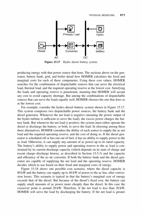
producing energy with that power source that hour. The sections above on the gen-

erator, battery bank, grid, and boiler detail how HOMER calculates the fixed and

marginal costs for each of these components. Using these cost values, HOMER

searches for the combination of dispatchable sources that can serve the electrical

load, thermal load, and the required operating reserve at the lowest cost. Satisfying

the loads and operating reserve is paramount, meaning that HOMER will accept

any cost to avoid capacity shortage. But among the combinations of dispatchable

sources that can serve the loads equally well, HOMER chooses the one that does so

at the lowest cost.

For example, consider the hydro–diesel–battery system shown in Figure 15.17.

This system comprises two dispatchable power sources, the battery bank and the

diesel generator. Whenever the net load is negative (meaning the power output of

the hydro turbine is sufficient to serve the load), the excess power charges the bat-

tery bank. But whenever the net load is positive, the system must either operate the

diesel or discharge the battery, or both, to serve the load. In choosing among these

three alternatives, HOMER considers the ability of each source to supply the ac net

load and the required operating reserve, and the cost of doing so. If the diesel gen-

erator is scheduled off or has run out of fuel, it has no ability to supply power to the

ac load. Otherwise, it can supply any amount of ac power up to its rated capacity.

The battery’s ability to supply power and operating reserve to the ac load is con-

strained by its current discharge capacity (which depends on its state of charge and

recent charge–discharge history, as described in Section 15.5.3) and the capacity

and efficiency of the ac–dc converter. If both the battery bank and the diesel gen-

erator are capable of supplying the net load and the operating reserve, HOMER

decides which to use based on their fixed and marginal costs of energy.

Figure 15.18 shows one possible cost scenario, where the diesel capacity is

80 kW and the battery can supply up to 40 kW of power to the ac bus, after conver-

sion losses. This scenario is typical in that the battery’s marginal cost of energy

exceeds that of the diesel. But because of the diesel’s fixed cost, the battery can

supply small amounts of ac power more cheaply than the diesel. In this case the

crossover point is around 20 kW. Therefore, if the net load is less than 20 kW,

HOMER will serve the load by discharging the battery. If the net load is greater

Figure 15.17 Hydro–diesel–battery system.


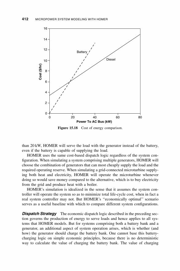
than 20 kW, HOMER will serve the load with the generator instead of the battery,

even if the battery is capable of supplying the load.

HOMER uses the same cost-based dispatch logic regardless of the system con-

figuration. When simulating a system comprising multiple generators, HOMER will

choose the combination of generators that can most cheaply supply the load and the

required operating reserve. When simulating a grid-connected microturbine supply-

ing both heat and electricity, HOMER will operate the microturbine whenever

doing so would save money compared to the alternative, which is to buy electricity

from the grid and produce heat with a boiler.

HOMER’s simulation is idealized in the sense that it assumes the system con-

troller will operate the system so as to minimize total life-cycle cost, when in fact a

real system controller may not. But HOMER’s ‘‘economically optimal’’ scenario

serves as a useful baseline with which to compare different system configurations.

Dispatch Strategy The economic dispatch logic described in the preceding sec-

tion governs the production of energy to serve loads and hence applies to all sys-

tems that HOMER models. But for systems comprising both a battery bank and a

generator, an additional aspect of system operation arises, which is whether (and

how) the generator should charge the battery bank. One cannot base this battery-

charging logic on simple economic principles, because there is no deterministic

way to calculate the value of charging the battery bank. The value of charging

0

2

4

6

8

10

12

14

16

0 20 40 60 80Power To AC Bus (kW)

Co

st (

$/h

r)

Battery

Diesel

Figure 15.18 Cost of energy comparison.


the battery in one hour depends on what happens in future hours. In a wind–diesel–

battery system, for example, charging the battery bank with diesel power in one

hour would be of some value if doing so allowed the system to avoid operating

the diesel in some subsequent hour. But it would be of no value whatsoever if

the system experienced more than enough excess wind power in subsequent hours

to charge the battery bank fully. In that case, any diesel power put into the battery

bank would be wasted because the wind power would have fully charged the battery

bank anyway.

Rather than using complicated probabilistic logic to determine the optimal

battery-charging strategy, HOMER provides two simple strategies and lets the user

model them both to see which is better in any particular situation. These dispatch

strategies are called load-following and cycle-charging. Under the load-following

strategy, a generator produces only enough power to serve the load, and does not

charge the battery bank. Under the cycle-charging strategy, whenever a generator

operates, it runs at its maximum rated capacity (or as close as possible without

incurring excess electricity) and charges the battery bank with the excess. Barley

and Winn [9] found that over a wide range of conditions, the better of these two

simple strategies is virtually as cost-effective as the ideal predictive strategy.

Because HOMER treats the dispatch strategy as a decision variable, the modeler

can easily simulate both strategies to determine which is optimal in a given

situation.

The dispatch strategy does not affect the decisions described in the preceding

section as to which dispatchable power sources operate each hour. Only after these

decisions are made does the dispatch strategy come into play. If the load-following

strategy applies, whichever generators HOMER selects to operate in a given hour

will produce only enough power to serve the load. If the cycle-charging strategy

applies, those same generators will run at their rated output, or as close as possible

without causing excess energy.

An optional control parameter called the set-point state of charge can apply to

the cycle-charging strategy. If the modeler chooses to apply this parameter, once the

generator starts charging the battery bank, it must continue to do so until the battery

bank reaches the set-point state of charge. Otherwise, HOMER may choose to dis-

charge the battery as soon as it can supply the load. The set-point state of charge

helps avoid situations where the battery experiences shallow charge–discharge

cycles near its minimum state of charge. In real systems, such situations are harmful

to battery life.

Load Priority HOMER makes a separate set of decisions regarding how to

allocate the electricity produced by the system. The presence of both an ac and

a dc bus complicates these decisions somewhat. HOMER assumes that electricity

produced on one bus will go first to serve primary load on the same bus, then pri-

mary load on the opposite bus, then deferrable load on the same bus, then defer-

rable load on the opposite bus, then to charge the battery bank, then to grid sales,

then to serve the electrolyzer, and then to the dump load, which optionally serves

the thermal load.


15.6 ECONOMIC MODELING

Economics play an integral role both in HOMER’s simulation process, wherein it

operates the system so as to minimize total net present cost, and in its optimization

process, wherein it searches for the system configuration with the lowest total net

present cost. This section describes why life-cycle cost is the appropriate metric

with which to compare the economics of different system configurations, why

HOMER uses the total net present cost as the economic figure of merit, and how

HOMER calculates total net present cost.

Renewable and nonrenewable energy sources typically have dramatically differ-

ent cost characteristics. Renewable sources tend to have high initial capital costs

and low operating costs, whereas conventional nonrenewable sources tend to

have low capital and high operating costs. In its optimization process, HOMER

must often compare the economics of a wide range of system configurations com-

prising varying amounts of renewable and nonrenewable energy sources. To be

equitable, such comparisons must account for both capital and operating costs.

Life-cycle cost analysis does so by including all costs that occur within the life

span of the system.

HOMER uses the total net present cost (NPC) to represent the life-cycle cost of a

system. The total NPC condenses all the costs and revenues that occur within the

project lifetime into one lump sum in today’s dollars, with future cash flows dis-

counted back to the present using the discount rate. The modeler specifies the dis-

count rate and the project lifetime. The NPC includes the costs of initial

construction, component replacements, maintenance, fuel, plus the cost of buying

power from the grid and miscellaneous costs such as penalties resulting from pol-

lutant emissions. Revenues include income from selling power to the grid, plus any

salvage value that occurs at the end of the project lifetime. With the NPC, costs are

positive and revenues are negative. This is the opposite of the net present value. As

a result, the net present cost is different from net present value only in sign.

HOMER assumes that all prices escalate at the same rate over the project life-

time. With that assumption, inflation can be factored out of the analysis simply by

using the real (inflation-adjusted) interest rate rather than the nominal interest rate

when discounting future cash flows to the present. The HOMER user therefore

enters the real interest rate, which is roughly equal to the nominal interest rate

minus the inflation rate. All costs in HOMER are real costs, meaning that they

are defined in terms of constant dollars.

For each component of the system, the modeler specifies the initial capital cost,

which occurs in year zero, the replacement cost, which occurs each time the com-

ponent needs replacement at the end of its lifetime, and the O&M cost, which

occurs each year of the project lifetime. The user specifies the lifetime of most com-

ponents in years, but HOMER calculates the lifetime of the battery and generators

as described in Section 15.5.3. A component’s replacement cost may differ from its

initial capital cost for several reasons. For example, a modeler might assume that a

wind turbine nacelle will need replacement after 15 years, but the tower and foun-

dation will last for the life of the project. In that case, the replacement cost would be


considerably less than the initial capital cost. Donor agencies or buy-down programs

might cover some or all of the initial capital cost of a PV array but none of the repla-

cement cost. In that case, the replacement cost may be greater than the initial capital

cost. When analyzing a retrofit of an existing diesel system, the initial capital cost of

the diesel engine would be zero, but the replacement cost would not.

To calculate the salvage value of each component at the end of the project life-

time, HOMER uses the equation

S ¼ Crep

Rrem

Rcomp

ð15:11Þ

where S is the salvage value, Crep the replacement cost of the component, Rrem the

remaining life of the component, and Rcomp the lifetime of the component. For

example, if the project lifetime is 20 years and the PV array lifetime is also 20 years,

the salvage value of the PV array at the end of the project lifetime will be zero

because it has no remaining life. On the other hand, if the PV array lifetime is

30 years, at the end of the 20-year project lifetime its salvage value will be one-third

of its replacement cost.

For each component, HOMER combines the capital, replacement, maintenance,

and fuel costs, along with the salvage value and any other costs or revenues, to find

the component’s annualized cost. This is the hypothetical annual cost that if it

occurred each year of the project lifetime would yield a net present cost equivalent

to that of all the individual costs and revenues associated with that component over

the project lifetime. HOMER sums the annualized costs of each component, along

with any miscellaneous costs, such as penalties for pollutant emissions, to find the

total annualized cost of the system. This value is an important one because HOMER

uses it to calculate the two principal economic figures of merit for the system: the

total net present cost and the levelized cost of energy.

HOMER uses the following equation to calculate the total net present cost:

CNPC ¼ Cann;tot

CRF i;Rproj

� � ð15:12Þ

where Cann;tot is the total annualized cost, i the annual real interest rate (the discount

rate), Rproj the project lifetime, and CRF( �) is the capital recovery factor, given by

the equation

CRF i;Nð Þ ¼ i 1 þ ið ÞN

1 þ ið ÞN�1ð15:13Þ

where i is the annual real interest rate and N is the number of years.

HOMER uses the following equation to calculate the levelized cost of energy:

COE ¼ Cann;tot

Eprim þ Edef þ Egrid;sales

ð15:14Þ

where Cann;tot is the total annualized cost, Eprim and Edef are the total amounts of

primary and deferrable load, respectively, that the system serves per year, and

ECONOMIC MODELING 415

Egrid;sales is the amount of energy sold to the grid per year. The denominator in equa-

tion (15.14) is an expression of the total amount of useful energy that the system

produces per year. The levelized cost of energy is therefore the average cost per

kilowatthour of useful electrical energy produced by the system.

Although the levelized cost of energy is often a convenient metric with which to

compare the costs of different systems, HOMER uses the total NPC instead as its

primary economic figure of merit. In its optimization process, for example,

HOMER ranks the system configurations according to NPC rather than levelized

cost of energy. This is because the definition of the levelized cost of energy is dis-

putable in a way that the definition of the total NPC is not. In developing the for-

mula that HOMER uses for the levelized cost of energy, we decided to divide by the

amount of electrical load that the system actually serves rather than the total elec-

trical demand, which may be different if the user allows some unmet load. We also

decided to neglect thermal energy but to include grid sales as useful energy produc-

tion. Each of these decisions is somewhat arbitrary, making the definition of the

levelized cost of energy also somewhat arbitrary. Because the total NPC suffers

from no such definitional ambiguity, it is preferable as the primary economic figure

of merit.

REFERENCES

[1] J. F. Manwell and J. G. McGowan, A combined probabilistic/time series model for wind

diesel systems simulation, Solar Energy, Vol. 53, pp. 481–490, 1994.

[2] Maui Solar Energy Software Corporation, PV-DesignPro, http://www.mauisolarsoftware.

com, accessed February 2, 2005.

[3] PV*SOL, http://www.valentin.de, accessed February 2, 2005.

[4] RETScreen International http://www.retscreen.net, accessed February 2, 2005.

[5] J. A. Duffie and W. A. Beckman, Solar Engineering of Thermal Processes 2nd ed., Wiley,

New York, 1991.

[6] F. M. White, Fluid Mechanics, 2nd ed., McGraw-Hill, New York, 1986.

[7] V. A. Graham and K. G. T. Hollands, A method to generate synthetic hourly solar

radiation globally, Solar Energy, Vol. 44, No. 6, pp. 333–341, 1990.

[8] J. F. Manwell and J. G. McGowan, Lead acid battery storage model for hybrid energy

systems, Solar Energy, Vol. 50, pp. 399–405, 1993.

[9] C. D. Barley and C. B. Winn, Optimal dispatch strategy in remote hybrid power systems,

Solar Energy, Vol. 58, pp. 165–179, 1996.

GLOSSARY

Annualized cost: the hypothetical annual cost value that if it occurred each year of

the project lifetime would yield a net present cost equivalent to the actual net

present cost. HOMER calculates the annualized cost of each system component

and of the entire system.


Autonomous: not connected to a larger power transmission grid. Autonomous

power systems are often called off-grid systems. An autonomous system must

be controlled carefully to match electrical supply and demand.

Battery energy cost: the average cost per kilowatthour of the energy stored in the

battery bank.

Battery wear cost: the cost per kilowatthour of cycling energy through the battery

bank. HOMER can calculate this value because it assumes that a certain amount

of energy can cycle through the battery bank before it needs replacement. Every

kilowatthour of energy that cycles through the battery bank reduces its life span

by a known amount.

Beam radiation: solar radiation that travels from the sun to Earth’s surface without

any scattering by the atmosphere. Beam radiation is also called direct radiation.

Capacity shortage: a shortfall that occurs between the required amount of operat-

ing capacity (load plus required operating reserve) and the actual operating capa-

city the system can provide.

Clearness index: the fraction of the solar radiation striking the top of the atmo-

sphere that makes it though the atmosphere to strike the surface of the Earth.

Constraint: a condition that system configurations must satisfy. HOMER discards

systems that do not satisfy the applicable constraints. For example, the HOMER

user may impose a constraint that all system configurations must serve at least

99% of the electrical demand over the year.

Decision variable: a variable over which the system designer has control, and for

which HOMER can consider multiple values in its optimization process. Examples

include the number of batteries in the system or the size of the ac–dc converter.

Demand rate: the fee the electric utility applies each month to the peak hourly grid

demand. If the demand rate is $5/kW per month and the peak hourly demand in

January is 75 kW, the demand charge for January will be $375.

Diffuse radiation: solar radiation that has been scattered by the atmosphere.

Dispatch strategy: a set of rules that controls how a system charges the battery bank.

Extraterrestrial radiation: the solar radiation striking the top of EARTH’s atmo-

sphere. One can calculate the quantity of extraterrestrial radiation precisely for

any location on earth at any time.

Feasibility: the state of being feasible or infeasible. A feasible system configuration

is one that satisfies the constraints imposed by the user. An infeasible system is

one that violates one or more constraints.

Grid power price: the price the utility charges for power purchased from the grid.

In HOMER, this price can vary according to month, day of the week, and time of

day.

Levelized cost of energy: the average cost per kilowatthour of electricity produced

by the system.

Life-cycle cost: the total cost of installing and operating a component or system

over a specified time span, typically many years.

GLOSSARY 417

Micropower system: a system that produces electrical and possibly thermal power

to serve a nearby load.

Net load: the load minus the renewable power available to serve the load.

Net metering: a billing scheme by which the utility charges a micropower sys-

tem operator for the net grid purchases (purchases minus sales) over the billing

period.

Operating capacity: the total amount of electrical generation capacity that is oper-

ating (and ready to produce electricity) at any one time. A generator that is not

operating provides no operating capacity. A 200-kW generator that is operating

provides 200 kW of operating capacity.

Operating reserve: surplus electrical generation capacity (above that required to

meet the current electric load) that is operating and able to respond instantly

to a sudden increase in the electric load or a sudden decrease in the renewable

power output.

Replacement cost: the cost of replacing a component at the end of its useful life-

time. The replacement cost may differ from the initial capital cost for several

reasons: only part of the component may need replacement, a donor organization

may cover the initial capital cost but not the replacement cost, fixed costs may be

shared among many components initially but not at the time of replacement, and

so on.

Residual flow: the minimum stream flow that must bypass the hydro turbine for

ecological purposes.

Search space: the set of all system configurations over which HOMER searches for

the optimum during the optimization process.

Sellback rate: the price the utility pays for power sold to the grid. In HOMER, this

value can vary according to month, day of the week, and time of day.

Sensitivity variable: an input variable for which the modeler enters multiple values

rather than just one.

System configuration: a combination of particular numbers and sizes of compo-

nents, plus an operating strategy that defines how those components work

together.

Unmet load: electrical load that the power system is unable to serve. Unmet load

occurs when the electrical demand exceeds the supply.


micropower system modeling with homer - pspb.org · chapter 15 micropower system modeling with...

Documents