mice: multivariate imputation by chained equations in r in r - draft.pdf · mice: multivariate...
TRANSCRIPT
JSS Journal of Statistical SoftwareMMMMMM YYYY, Volume VV, Issue II. http://www.jstatsoft.org/
MICE: Multivariate Imputation by Chained
Equations in R
Stef van Buuren
1 TNO Quality of Life, Leiden2 University of Utrecht
Karin Groothuis-Oudshoorn
1 Roessingh RD, Enschede2 University Twente
Abstract
Multivariate Imputation by Chained Equations (MICE) is the name of software forimputing incomplete multivariate data by Fully Conditional Specification (FCS). MICEV1.0 appeared in the year 2000 as an S-PLUS library, and in 2001 as an R package. MICEV1.0 introduced predictor selection, passive imputation and automatic pooling. Thisarticle presents MICE V2.0, which extends the functionality of MICE V1.0 in several ways.In MICE V2.0, the analysis of imputed data is made completely general, whereas the rangeof models under which pooling works is substantially extended. MICE V2.0 adds newfunctionality for imputing multilevel data, automatic predictor selection, data handling,post-processing imputed values, specialized pooling and model selection. Imputation ofcategorical data is improved in order to bypass problems caused by perfect prediction.Special attention to transformations, sum scores, indices and interactions using passiveimputation, and to the proper setup of the predictor matrix. MICE V2.0 is freely availablefrom CRAN as an R package mice. This article provides a hands-on, stepwise approachto using mice for solving incomplete data problems in real data.
Keywords: multiple imputation, chained equations, fully conditional specification, gibbs sam-pler, predictor selection, passive imputation, R.
1. Introduction
Multiple imputation (Rubin 1987, 1996) is the method of choice for complex incomplete dataproblems. Missing data that occur in more than one variable presents a special challenge.Two general approaches for imputing multivariate data have emerged: joint modeling (JM)and fully conditional specification (FCS) (van Buuren 2007). Schafer (1997) developed var-ious JM techniques for imputation under the multivariate normal, the log-linear, and the

2 MICE: Multivariate Imputation by Chained Equations
general location model. JM involves specifying a multivariate distribution for the missingdata, and drawing imputation from their conditional distributions by Markov Chain MonteCarlo (MCMC) techniques. This methodology is attractive if the multivariate distribution isa reasonable description of the data. FCS specifies the multivariate imputation model on avariable-by-variable basis by a set of conditional densities, one for each incomplete variable.Starting from an initial imputation, FCS draws imputations by iterating over the conditionaldensities. A low number of iterations (say 10-20) is often sufficient. FCS is attractive as analternative to JM in cases where no suitable multivariate distribution can be found. The basicidea of FCS is already quite old, and has been proposed using a variety of names: stochas-tic relaxation (Kennickell 1991), variable-by-variable imputation (Brand 1999), regressionswitching (van Buuren et al. 1999), sequential regressions (Raghunathan et al. 2001), orderedpseudo-Gibbs sampler (Heckerman et al. 2001), partially incompatible MCMC (Rubin 2003),iterated univariate imputation (Gelman 2004), chained equations van Buuren and Oudshoorn(2000) and fully conditional specification (van Buuren 2007).
Software implementations
Several authors have implemented fully conditionally specified models for imputation. MICE(van Buuren and Oudshoorn 2000) was released as an S-PLUS library in 2000, and wasconverted by several users into R. IVEWARE (Raghunathan et al. 2001) is a SAS-basedprocedure that was independently developed by Raghunathan and colleagues. The functionaRegImpute in R and S Plus is part of the Hmisc package Harrell (2001). The ice software(Royston 2004, 2005) is a widely used implementation in STATA. SOLAS 3.0 (Solutions 2001)is also based on conditional specification, but does not iterate. WinMICE (Jacobusse 2005)is a Windows stand-alone program for generating imputations under the hierarchical linearmodel. A recent addition is the R package mi (Su et al. 2009). Furthermore, FCS is nowwidely available through the multiple imputation procedure part of the SPSS V17 moduleMVA. See http://www.multiple-imputation.com for an overview.
Applications of Chained Equations
Applications of imputation by chained equations have now appeared in quite diverse fields:addiction (Schnoll et al. 2006; Macleod et al. 2008; Adamczyk and Palmer 2008; Caria et al.2009; Morgenstern et al. 2009), arthritis and rheumatology (Wolfe et al. 2006; Rahman et al.2008; Van Den Hout et al. 2009), atherosclerosis (Tiemeier et al. 2004; Van Oijen et al. 2007;McClelland et al. 2008), cardiovascular system (Ambler et al. 2005; van Buuren et al. 2006a;Chase et al. 2008; Byrne et al. 2009; Klein et al. 2009), cancer (Clark et al. 2001, 2003; Clarkand Altman 2003; Royston et al. 2004; Barosi et al. 2007; Fernandes et al. 2008; Sharma et al.2008; McCaul et al. 2008; Huo et al. 2008; Gerestein et al. 2009), epidemiology (Cummingset al. 2006; Hindorff et al. 2008; Mueller et al. 2008; Ton et al. 2009), endocrinology (Rouxelet al. 2004; Prompers et al. 2008), infectious diseases (Cottrell et al. 2005; Walker et al.2006; Cottrell et al. 2007; Kekitiinwa et al. 2008; Nash et al. 2008; Sabin et al. 2008; Theinet al. 2008; Garabed et al. 2008; Michel et al. 2009), genetics (Souverein et al. 2006), healtheconomics (Briggs et al. 2003; Burton et al. 2007; Klein et al. 2008; Marshall et al. 2009),obesity and physical activity (Orsini et al. 2008a; Wiles et al. 2008; Orsini et al. 2008b;Van Vlierberghe et al. 2009), pediatrics and child development (Hill et al. 2004; Mumtazet al. 2007; Deave et al. 2008; Samant IV et al. 2008; Butler and Heron 2008; Ramchandaniet al. 2008; Van Wouwe et al. 2009), rehabilitation (van der Hulst et al. 2008), behavior

Journal of Statistical Software 3
(Veenstra et al. 2005; Melhem et al. 2007; Horwood et al. 2008; Rubin et al. 2008), qualityof care (Sisk et al. 2006; Roudsari et al. 2007; Ward and Franks 2007; Grote et al. 2007;Roudsari et al. 2008; Grote et al. 2008; Sommer et al. 2009), human reproduction (Smithet al. 2004a,b; Hille et al. 2005; Alati et al. 2006; O’Callaghan et al. 2006; Hille et al. 2007;Den Hartog et al. 2008), management sciences (Jensen and Roy 2008), occupational health(Heymans et al. 2007; Brunner et al. 2007; Chamberlain et al. 2008), politics (Tanasoiu andColonescu 2008), psychology (Sundell et al. 2008) and sociology (Finke and Adamczyk 2008).All authors use some form of chained equations to handle the missing data, but the detailsvary considerably. The interested reader could check out articles from a familiar applicationarea to see how multiple imputation is done and reported.
MICE
This paper describes the R package mice. The package contains functions for three phasesof multiple imputation: generating multiple imputation, analyzing imputed data, and forpooling analysis results. Specific features of the software are:
� columnwise specification of the imputation model
� arbitrary patterns of missing data
� passive imputation
� subset selection of predictors
� support of arbitrary complete-data methods
� support pooling various types of statistics
� diagnostics of imputations
� callable user-written imputation functions
Package mice V2.0 replaces version V1.21, but is fully compatible with previous versions.This document replaces the original manual (van Buuren and Oudshoorn 2000). MICE V2.0extends MICE V1.0 in several ways. New in V2.0 is:
� quickpred() for automatic generation of the predictor matrix
� mice.impute.2l.norm() for imputing multilevel data
� stable imputation of categorical data
� post-processing imputations through the post argument
� with.mids() for general data analysis on imputed data
� pool.scalar() and pool.r.squared() for specialized pooling
� pool.compare() for model testing on imputed data
� cbind.mids(), rbind.mids() and ibind() for combining imputed data

4 MICE: Multivariate Imputation by Chained Equations
Furthermore, this document introduces a new strategy to specify the predictor matrix inconjunction with passive imputation. The amount and scope of example code has beenexpanded considerably. All programming code used in this paper is available in the file\doc\JSScode.R of the mice package.
The intended audience of this paper consists of applied researchers who want to address prob-lems caused by missing data by multiple imputation. The text assumes basic familiarity withR. The document contains hands-on analysis using the mice package. We do not discuss prob-lems of incomplete data in general. We refer to the excellent books by Little and Rubin (2002)and Schafer (1997). Theory and applications of multiple imputation have been developed inRubin (1987) and Rubin (1996).
Package mice V2.0 was written in pure R using old-style S3 classes and methods. MICE V2.0was written and tested in R 2.9.1. The package has a simple architecture, is highly modular,and allows easy access to all program code from within the R environment.
2. General framework
To the uninitiated, multiple imputation is a bewildering technique that differs substantiallyfrom conventional statistical approaches. As a result, the first-time user may get lost ina labyrinth of imputation models, missing data mechanisms, multiple versions of the data,pooling, and so on. This section describes a modular approach to multiple imputation thatforms the basis of the architecture of MICE. The philosophy behind MICE is that multipleimputation is best done as a sequence of small steps, each of which may require diagnosticchecking. Our hope is that the framework will aid the user to map out the steps needed inpractical applications.
2.1. Notation
Let Yj with (j = 1, . . . , p) be one of p incomplete variables, where Y = (Y1, . . . , Yp). Theobserved and missing parts of Yj are denoted by Y obs
j and Y misj , respectively, so Y obs =
(Y obs1 , . . . , Y obs
p ) and Y mis = (Y mis1 , . . . , Y mis
p ) stand for the observed and missing data in Y .
The number of imputation is equal to m ≥ 1. The ℎth imputed data sets is denoted as Y (ℎ)
where ℎ = 1, . . . ,m. Let Y−j = (Y1, . . . , Yj−1, Yj+1, . . . , Yp) denote the collection of the p− 1variables in Y except Yj . Let Q denote the quantity of scientific interest (e.g. a regressioncoefficient). In practice, Q is often a multivariate vector. More generally, Q encompasses anymodel of scientific interest.
2.2. Modular approach to Multiple Imputation
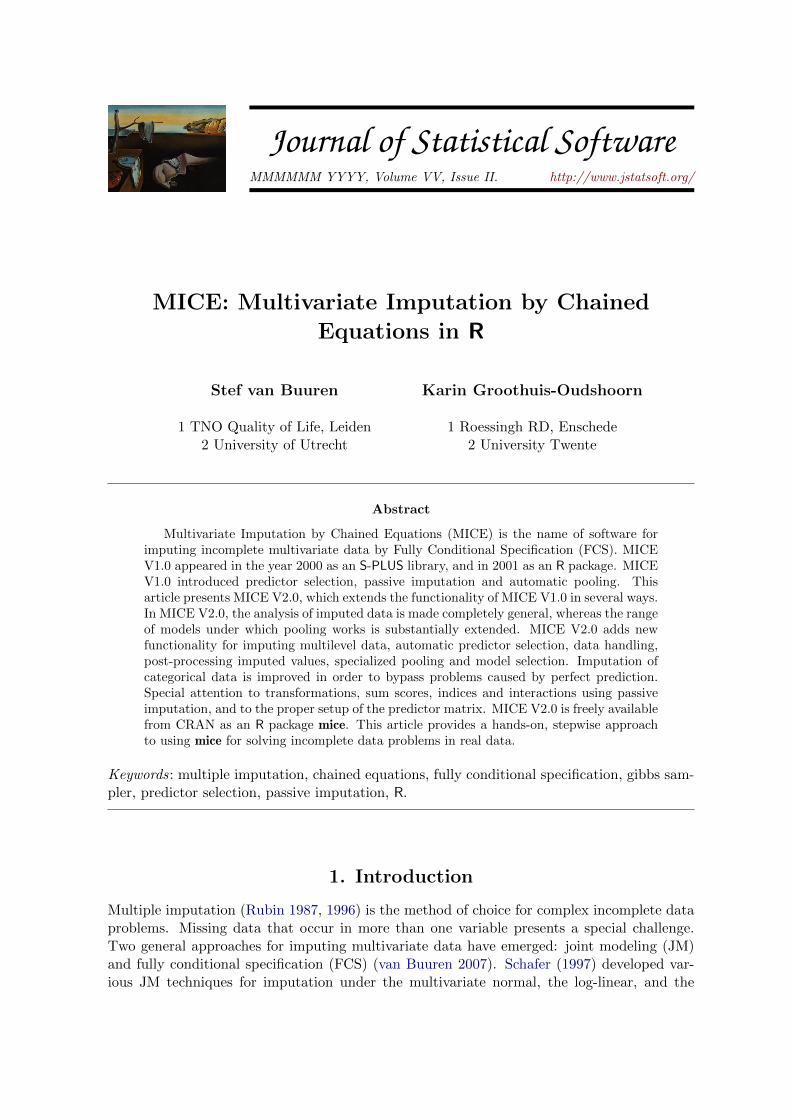
Figure 1 illustrates the three main steps in multiple imputation: imputation, analysis andpooling. The software stores the results of each step in a specific class: mids, mira and mipo.We now explain each of these in more detail.
The leftmost side of the picture indicates that the analysis starts with an observed, incom-plete data set Yobs. In general, the problem is that we cannot estimate Q from Yobs withoutmaking unrealistic assumptions about the unobserved data. Multiple imputation is a generalframework that several imputed versions of the data by replacing the missing values by plau-sible data values. These plausible values are drawn from a distribution specifically modeled
Journal of Statistical Software 5
incomplete data imputed data analysis results pooled results
data frame mids mira mipo
mice() with() pool()
Figure 1: Main steps used in multiple imputation.
for each missing entry. In MICE this task is being done by the function mice(). Figure 1portrays m = 3 imputed data sets Y (1), . . . , Y (3). The three imputed sets are identical for thenon-missing data entries, but differ in the imputed values. The magnitude of these differencereflects our uncertainty about what value to impute. The package has a special class forstoring the imputed data: a multiply imputed dataset of class mids.
The second step is to estimate Q on each imputed data set, typically by the method wewould have used if the data had been complete. This is easy since all data are now complete.The model applied to Y (1), . . . , Y (m) is the generally identical. MICE 2.0 contains a func-tion with.mids() that perform this analysis. This function supersedes the lm.mids() andglm.mids(). The estimates Q(1), . . . , Q(m) will differ from each other because their input datadiffer. It is important to realize that these differences are caused because of our uncertaintyabout what value to impute. In MICE the analysis results are collectively stored as a multiplyimputed repeated analysis within an R object of class mira.
The last step is to pool the m estimates Q(1), . . . , Q(m) into one estimate Q and estimate itsvariance. For quantities Q that are approximately normally distributed, we can calculate themean over Q(1), . . . , Q(m) and sum the within- and between-imputation variance accordingto the method outlined in Rubin (1987, pp. 76–77). The function pool() contains methodsfor pooling quantities by Rubin’s rules. The results of the function is stored as a multipleimputed pooled outcomes object of class mipo.
2.3. Chained Equations
The imputation model should
� account for the process that created the missing data,
� preserve the relations in the data, and
� preserve the uncertainty about these relations.

6 MICE: Multivariate Imputation by Chained Equations
The hope is that adherence to these principles will yield imputations that are statisticallycorrect as in Rubin (1987, chap. 4) for a wide range in Q. Typical problems that may surfacewhile imputing multivariate missing data are
� For a given Yj , predictors Y−j used in the imputation model may themselves be incom-plete;
� Circular” dependence can occur, where Y1 depends on Y2 and Y2 depends on Y1 becausein general Y1 and Y2 are correlated, even given other variables;
� Especially with large p and small n, collinearity and empty cells may occur;
� Rows or columns can be ordered, e.g., as with longitudinal data;
� Variables can be of different types (e.g., binary, unordered, ordered, continuous), therebymaking the application of theoretically convenient models, such as the multivariatenormal, theoretically inappropriate;
� The relation between Yj and Y−j could be complex, e.g., nonlinear, or subject to cen-soring processes;
� Imputation can create impossible combinations (e.g. pregnant fathers), or destroy de-terministic relations in the data (e.g. sum scores);
� Imputations can be nonsensical (e.g. body temperature of the dead);
� Models for Q that will be applied to the imputed data may not (yet) be known.
This list is by no means exhaustive, and other complexities may appear for particular data.
In order to address the issues posed by the real-life complexities of the data, it is convenientto specify the imputation model separately for each column in the data. This has led by tothe development of the technique of chained equations. Specification occurs on at a level thatis well understood by the user, i.e., at the variable level. Moreover, techniques for creatingunivariate imputations have been well developed.
Let the hypothetically complete data Y be a partially observed random sample from the p-variate multivariate distribution P (Y ∣�). We assume that the multivariate distribution of Yis completely specified by �, a vector of unknown parameters. The problem is how to get themultivariate distribution of �, either explicitly or implicitly. The chained equations proposesto obtain a posterior distribution of � by sampling iteratively from conditional distributionsof the form
P (Y1∣Y−1, �1)
...
P (Yp∣Y−p, �p).
The parameters �1, . . . , �p are specific to the respective conditional densities and are notnecessarily the product of a factorization of the ”true” joint distribution P (Y ∣�). Starting from

Journal of Statistical Software 7
a simple draw from observed marginal distributions, the tth iteration of chained equations isa Gibbs sampler that successively draws
�∗(t)1 ∼ P (�1∣Y obs
1 , Y(t−1)2 , . . . , Y (t−1)
p )
Y∗(t)1 ∼ P (Y1∣Y obs
1 , Y(t−1)2 , . . . , Y (t−1)
p , �∗(t)1 )
...
�∗(t)p ∼ P (�p∣Y obsp , Y
(t)1 , . . . , Y
(t)p−1)
Y ∗(t)p ∼ P (Yp∣Y obs
p , Y(t)1 , . . . , Y (t)
p , �∗(t)p )
where Y(t)j = (Y obs
j , Y∗(t)j ) is the jth imputed variable at iteration t. Observe that previous
imputations Y∗(t−1)j only enter Y
∗(t)j through its relation with other variables, and not directly.
Convergence can therefore be quite fast, unlike many other MCMC methods. It is importantto monitor convergence, but in our experience the number of iterations can often be a smallnumber, say 10–20. The name chained equations refers to the fact that the Gibbs sampler canbe easily implemented as a concatenation of univariate procedures to fill out the missing data.The mice() function executes m streams in parallel, each of which generates one imputeddata set.
The chained equations algorithm possesses a touch of magic. The method has been foundto work well in a variety of simulation studies (Brand 1999; Horton and Lipsitz 2001; Moonset al. 2006; van Buuren et al. 2006b; Horton and Kleinman 2007; Yu et al. 2007; Schunk 2008;Drechsler and Rassler 2008; Giorgi et al. 2008). Note that it is possible to specify models forwhich no known joint distribution exits. Two linear regressions specify a joint multivariatenormal given specific regularity condition (Arnold and Press 1989). However, the joint distri-bution of one linear and, say, one proportional odds regression model is unknown, yet very easyto specify in MICE. The conditionally specified model may be incompatible in the sense thatthe joint distribution cannot exist. It is not yet clear what the consequences of incompatibilityare on the quality of the imputations. The little simulation work that is available suggeststhat the problem is probably not serious in practice (van Buuren et al. 2006b; Drechsler andRassler 2008). Compatible multivariate imputation models (Schafer 1997) have been foundto work in a large variety of cases, but may lack flexibility to address specific features of thedata. Gelman and Raghunathan (2001) remark that ’separate regressions often make moresense than joint models’. In order to bypass the limitations of joint models, Gelman (2004,pp. 541) concludes: ’Thus we are suggesting the use of a new class of models—inconsistentconditional distributions—that were initially motivated by computational and analytical con-venience.’ As a safeguard to evade potential problems by incompatibility, we suggest thatthe order in which variable are imputed should be sensible. This ordering can be specified inMICE (c.f. section 3.6). Existence and uniqueness theorems for conditionally specified modelshave been derived (Arnold and Press 1989; Arnold et al. 1999; Ip and Wang 2009). More workalong these lines would be useful in order to identify the boundaries at which the algorithmbreaks down. Barring this, chained equations seem to work well in many examples, is of greatimportance in practice, and is easily applied.
2.4. Simple example
The section presents a simple example incorporating all three steps. After installing the R

8 MICE: Multivariate Imputation by Chained Equations
package mice from CRAN, load the package.
> library(mice)
Loading required package: MASS
Loading required package: nnet
Loading required package: nlme
The data frame nhanes contains data from Schafer (1997, p. 237). The data contains four vari-ables: age (age group), bmi (body mass index), hyp (hypertension status) and chl (cholesterollevel). The data are stored as a data frame. Missing values are represented as NA.
> nhanes
age bmi hyp chl
1 1 NA NA NA
2 2 22.7 1 187
3 1 NA 1 187
4 3 NA NA NA
5 1 20.4 1 113
...
Inspecting the missing data
The number of the missing values can be counted and visualized as follows:
> md.pattern(nhanes)
age hyp bmi chl
13 1 1 1 1 0
1 1 1 0 1 1
3 1 1 1 0 1
1 1 0 0 1 2
7 1 0 0 0 3
0 8 9 10 27
There are 13 (out of 25) rows that are complete. There is one row for which only bmi ismissing, and there are seven rows for which only age is known. The total number of missingvalues is equal to (7× 3) + (1× 2) + (3× 1) + (1× 1) = 27. Most missing values (10) occurin chl.
Another way to study the pattern involves calculating the number of observations per patternsfor all pairs of variables. A pair of variables can have exactly four missingness patterns: bothvariables are observed (pattern rr), the first variable is observed and the second variable ismissing (pattern rm), the first variable is missing and the second variable is observed (patternmr), and both are missing (pattern mm). We can use the md.pairs() function to calculate thefrequency in each pattern for all variable pairs as

Journal of Statistical Software 9
> p <- md.pairs(nhanes)
> p
$rr
age bmi hyp chl
age 25 16 17 15
bmi 16 16 16 13
hyp 17 16 17 14
chl 15 13 14 15
$rm
age bmi hyp chl
age 0 9 8 10
bmi 0 0 0 3
hyp 0 1 0 3
chl 0 2 1 0
$mr
age bmi hyp chl
age 0 0 0 0
bmi 9 0 1 2
hyp 8 0 0 1
chl 10 3 3 0
$mm
age bmi hyp chl
age 0 0 0 0
bmi 0 9 8 7
hyp 0 8 8 7
chl 0 7 7 10
Thus, for pair (bmi,chl) there are 13 completely observed pairs, 3 pairs for which bmi isobserved but hyp not, 2 pairs for which bmi is missing but with hyp observed, and 7 pairswith both missing bmi and hyp. Note that these numbers add up to the total sample size.
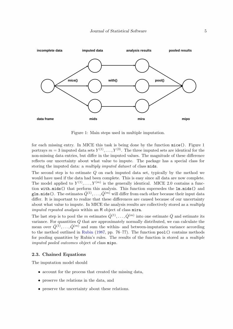
The R package VIM (Templ and Filzmoser 2008) contains functions for plotting incompletedata. The margin plot of the pair (bmi,chl) can be plotted by
> library(VIM)
> marginplot(nhanes[,c("chl","bmi")], col=c("blue","red","orange"), cex=1.5,
+ cex.lab=1.5, cex.numbers=1.3, pch=19)
Figure 2 displays the result. The data area holds 13 blue points for which both bmi and chl
were observed. The three red dots in the left margin correspond to the records for whichbmi is observed and chl is missing. The points are drawn at the known values of bmi at24.9, 25.5 and 29.6. Likewise, the bottom margin contain two red points with observed chl
and missing bmi. The orange dot at the intersection of the bottom and left margin indicates
10 MICE: Multivariate Imputation by Chained Equations
9
107
150 200 250
2025
3035
chl
bmi
Figure 2: Margin plot of bmi versus chl as drawn by the marginplot() function in the VIMpackage. Observed data in blue, missing data in red.
that there are also records for which both bmi and chl is missing. The three numbers at thelower left corner indicate the number of incomplete records for various combinations. Thereare 9 records in which bmi is missing, 10 records in which chl is missing, and 7 records inwhich both are missing. Furthermore, the left margin contain two box plots, a blue and ared one. The blue box plot in the left margin summarizes the marginal distribution of bmiof the 13 blue points. The red box plot summarizes the distribution of the three bmi valueswith missing chl. Under MCAR, these distribution are expected to be identical. Likewise,the two colored box plots in the bottom margin summarize the respective distributions forcodechl.
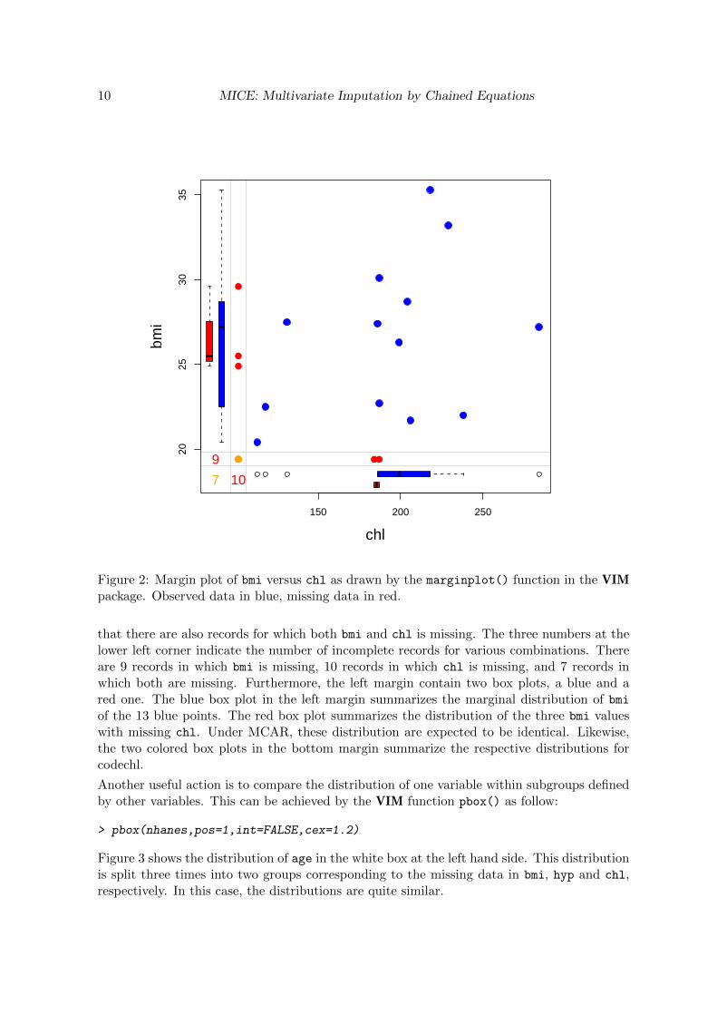
Another useful action is to compare the distribution of one variable within subgroups definedby other variables. This can be achieved by the VIM function pbox() as follow:
> pbox(nhanes,pos=1,int=FALSE,cex=1.2)
Figure 3 shows the distribution of age in the white box at the left hand side. This distributionis split three times into two groups corresponding to the missing data in bmi, hyp and chl,respectively. In this case, the distributions are quite similar.
Journal of Statistical Software 11
25 16 9 17 8 15 100 0 0 0 0 0 0
obs.
in b
mi
mis
s. in
bm
i
obs.
in h
yp
mis
s. in
hyp
obs.
in c
hl
mis
s. in
chl
1.0
1.5
2.0
2.5
3.0
age
Figure 3: Distribution of age for different patterns of missing data in bmi, hyp and chl.Observed data in blue, missing data in red.
Creating imputations
Creating imputations can be done with a call to mice() as follows:
> imp <- mice(nhanes)
iter imp variable
1 1 bmi hyp chl
1 2 bmi hyp chl
1 3 bmi hyp chl
1 4 bmi hyp chl
1 5 bmi hyp chl
2 1 bmi hyp chl
2 2 bmi hyp chl
...
where the multiply imputed data set is stored in the object imp of class mids. Inspect whatthe result looks like
12 MICE: Multivariate Imputation by Chained Equations
> imp
Multiply imputed data set
Call:
mice(data = nhanes)
Number of multiple imputations: 5
Missing cells per column:
age bmi hyp chl
0 9 8 10
Imputation methods:
age bmi hyp chl
"" "pmm" "pmm" "pmm"
VisitSequence:
bmi hyp chl
2 3 4
PredictorMatrix:
age bmi hyp chl
age 0 0 0 0
bmi 1 0 1 1
hyp 1 1 0 1
chl 1 1 1 0
Random generator seed value: NA
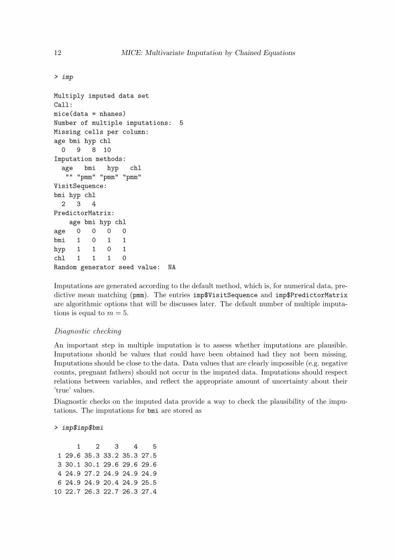
Imputations are generated according to the default method, which is, for numerical data, pre-dictive mean matching (pmm). The entries imp$VisitSequence and imp$PredictorMatrix
are algorithmic options that will be discusses later. The default number of multiple imputa-tions is equal to m = 5.
Diagnostic checking
An important step in multiple imputation is to assess whether imputations are plausible.Imputations should be values that could have been obtained had they not been missing.Imputations should be close to the data. Data values that are clearly impossible (e.g. negativecounts, pregnant fathers) should not occur in the imputed data. Imputations should respectrelations between variables, and reflect the appropriate amount of uncertainty about their’true’ values.
Diagnostic checks on the imputed data provide a way to check the plausibility of the impu-tations. The imputations for bmi are stored as
> imp$imp$bmi
1 2 3 4 5
1 29.6 35.3 33.2 35.3 27.5
3 30.1 30.1 29.6 29.6 29.6
4 24.9 27.2 24.9 24.9 24.9
6 24.9 24.9 20.4 24.9 25.5
10 22.7 26.3 22.7 26.3 27.4

Journal of Statistical Software 13
11 30.1 29.6 29.6 27.5 30.1
12 22.7 26.3 28.7 26.3 26.3
16 30.1 30.1 33.2 33.2 27.5
21 33.2 20.4 30.1 20.4 33.2
Each row corresponds to a missing entry in bmi. The columns contain the multiple imputa-tions. The actual results may vary.
The complete data combine observed and imputed data. The (first) completed data set canbe obtained as
> complete(imp)
age bmi hyp chl
1 1 29.6 1 187
2 2 22.7 1 187
3 1 30.1 1 187
4 3 24.9 1 184
5 1 20.4 1 113
...
The missing entries in nhanes have now been filled by the values from the first (of five)imputation. The second completed data set can be obtained by complete(imp,2). For theobserved data, it is identical to the first completed data set, but it may differ in the imputeddata.
It is often useful to inspect the distributions of original and the imputed data. One way ofdoing this is to use the function stripplot() from the package lattice to the imputed data.
> library(lattice)
> com <- complete(imp, "long", inc=T)
> col <- rep(c("blue","red")[1+as.numeric(is.na(imp$data$chl))],6)
> stripplot(chl˜.imp, data=com, jit=TRUE, fac=0.8, col=col, pch=20,
+ cex=1.4, xlab="Imputation number")
The complete() function extracts the original and five imputed data sets from the imp objectas a long (row-stacked) matrix with 150 record (25 original records, followed by five completeddata sets). The col vector separates the observed (blue) and imputed (red) data for chl.
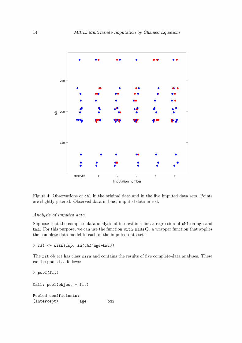
Figure 4 graphs the data values of chl before and after imputation. Imputations are plottedin red. Since the pmm method draws imputations from the observed data, imputed values havethe same gaps as in the observed data, and are always within the range of the observed data.Figure 4 indicates that the distributions of the imputed and the observed values are similar.The observed data have a particular feature that, for some reason, the data cluster aroundthe value of 187. The imputations reflects this feature, and are close to the data.
Under MCAR, univariate distributions of the observed and imputed data are expected tobe identical. Under MAR, they can be different, both in location and spread, but theirmultivariate distribution is assumed to be identical. There are many other ways to look atthe completed data, but we defer of a discussion of those to section 4.5.
14 MICE: Multivariate Imputation by Chained Equations
Imputation number
chl
150
200
250
observed 1 2 3 4 5
Figure 4: Observations of chl in the original data and in the five imputed data sets. Pointsare slightly jittered. Observed data in blue, imputed data in red.
Analysis of imputed data
Suppose that the complete-data analysis of interest is a linear regression of chl on age andbmi. For this purpose, we can use the function with.mids(), a wrapper function that appliesthe complete data model to each of the imputed data sets:
> fit <- with(imp, lm(chl˜age+bmi))
The fit object has class mira and contains the results of five complete-data analyses. Thesecan be pooled as follows:
> pool(fit)
Call: pool(object = fit)
Pooled coefficients:
(Intercept) age bmi

Journal of Statistical Software 15
-39.142978 36.764422 6.197402
Fraction of information about the coefficients missing due to nonresponse:
(Intercept) age bmi
0.1429260 0.2200509 0.1663141
More detailed output can be obtained, as usual, with the summary() function, i.e.,
> summary(pool(fit))
est se t df Pr(>|t|)
(Intercept) -39.142978 59.466728 -0.6582332 17.58143 0.518915406
age 36.764422 9.609663 3.8257764 14.65264 0.001718744
bmi 6.197402 1.875192 3.3049426 16.68720 0.004270331
lo 95 hi 95 missing fmi
(Intercept) -164.291480 86.00552 NA 0.1429260
age 16.239538 57.28931 0 0.2200509
bmi 2.235436 10.15937 9 0.1663141
>
This table contains the results that can be reported. After multiple imputation, we finda significant effect for both age and bmi. The column fmi contains the fraction of missinginformation, i.e. the proportion of the variability that is attributable to the uncertainty causedby the missing data. Note that the actual results obtained may differ since they will dependon the seed argument of the mice() function.
3. Imputation Models
3.1. Seven Choices
The specification of the imputation model is the most challenging step in multiple imputation.What are the choices that we need to make, and in what order? There are seven main choices:
1. First, we should decide whether the Missing at Random (MAR) assumption Rubin(1976) is plausible. The MAR assumption is a suitable starting point in many practicalcases, but there are also cases where the assumption is suspect. Schafer (1997, pp.20–23) provides a good set of practical examples. MICE can handle both MAR andMissing Not at Random (MNAR). Multiple imputation under MNAR requires additionalmodeling assumptions that influence the generated imputations. There are many waysto do this. We refer to section 6.2 for an example of how that could be realized.
2. The second choice refers to the form of the imputation model. The form encompassesboth the structural part and the assumed error distribution. Within MICE the formneeds to be specified for each incomplete column in the data. The choice will be steered

16 MICE: Multivariate Imputation by Chained Equations
by the scale of the dependent variable (i.e. the variable to be imputed), and preferablyincorporates knowledge about the relation between the variables. Section 3.2 describesthe possibilities within MICE.
3. Our third choice concerns the set of variables to include as predictors into the imputationmodel. The general advice is to include as many relevant variables as possible includingtheir interactions (Collins et al. 2001). This may however lead to unwieldy modelspecifications that could easily get out of hand. Section 3.3 describes the facilitieswithin MICE for selecting the predictor set.
4. The fourth choice is whether we should impute variables that are functions of other(incomplete) variables. Many data sets contain transformed variables, sum scores, in-teraction variables, ratio’s, and so on. It can be useful to incorporate the transformedvariables into the multiple imputation algorithm. Section 3.4 describes how MICE dealswith this situation using passive imputation.
5. The fifth choice concerns the order in which variables should be imputed. Severalstrategies are possible, each with their respective pro’s and cons. Section 3.6 shows howthe visitation scheme of the Gibbs sampler within MICE is under control of the user.
6. The sixth choice concerns the setup of the starting imputations and the number ofiterations. The convergence of the Gibbs sampler can be monitored in many ways.Section 4.3 outlines some techniques in MICE that assist in this task.
7. The seventh choice is m, the number of multiply imputed data sets. Setting m too lowleads to undercoverage and to P -values that are too low.
Please realize that these choices are always needed. The analysis in section 2.4 imputed thenhanes data using just a minimum of specifications and relied on MICE defaults. However,these default choices are not necessarily the best for your data. There is no magical settingthat produces appropriate imputations in every problem. Real problems need tailoring. It isour hope that the software will invite you to go beyond the default settings.
3.2. Elementary Imputation Methods
In MICE one specifies an elementary (=univariate) imputation model of each incompletevariable. Both the structural part of the imputation model and the error distribution needto be specified. The choice will depend on, amongst others, the scale of the variable tobe imputed. The univariate imputation method takes a set of (at that moment) completepredictors, and returns a single imputation for each missing entry in the incomplete targetcolumn. The mice package supplies a number of built-in elementary imputation models.These all have names mice.impute.name, where name identifies the elementary imputationmethod.
Table 1 contains the list of built-in imputation functions. The default methods are indicated.The method argument of mice() specifies the imputation method per column and overridesthe default. If method is specified as one string, then all visited data columns (c.f. section 3.6)will be imputed by the elementary function indicated by this string. So
> imp <- mice(nhanes, method = "norm")

Journal of Statistical Software 17
Method Description Scale type Default
pmm Predictive mean matching numeric Ynorm Bayesian linear regression numericnorm.nob Linear regression, non-Bayesian numericmean Unconditional mean imputation numeric2l.norm Two-level linear model numericlogreg Logistic regression factor, 2 levels Ypolyreg Polytomous (unordered) regression factor, >2 levels Ylda Linear discriminant analysis factorsample Random sample from the observed data any
Table 1: Built-in elementary imputation techniques. The techniques are coded as functionsnamed mice.impute.pmm(), and so on.
specifies that the function mice.impute.norm() is called for all columns. Alternatively,method can be a vector of strings of length ncol(data) specifying the function that is appliedto each column. Columns that need not be imputed have method "". For example,
> imp <- mice(nhanes, meth = c("", "norm", "pmm", "mean"))
applies different methods for different columns. The nhanes2 data frame contains one poly-tomous, one binary and two numeric variables.
> str(nhanes2)
'data.frame': 25 obs. of 4 variables:
$ age: Factor w/ 3 levels "1","2","3": 1 2 1 3 1 3 1 1 2 2 ...
$ bmi: num NA 22.7 NA NA 20.4 NA 22.5 30.1 22 NA ...
$ hyp: Factor w/ 2 levels "1","2": NA 1 1 NA 1 NA 1 1 1 NA ...
$ chl: num NA 187 187 NA 113 184 118 187 238 NA ...
Imputations can be created as
> imp <- mice(nhanes2, me=c("polyreg","pmm","logreg","norm"))
iter imp variable
1 1 bmi hyp chl
1 2 bmi hyp chl
1 3 bmi hyp chl
1 4 bmi hyp chl
1 5 bmi hyp chl
2 1 bmi hyp chl
...
where function mice.impute.polyreg() is used to impute the first (categorical) variable age,mice.impute.ppm() for the second numeric variable bmi, function mice.impute.logreg()
for the third binary variable hyp and function mice.impute.norm() for the numeric variable

18 MICE: Multivariate Imputation by Chained Equations
chl. The me parameter is a legal abbreviation of the method argument. As age did notcontain any missing data, it is not mentioned in the output.
Empty imputation method
MICE will automatically skip imputation of variables that are complete. One of the problemsin previous versions of MICE was that all incomplete data needed to be imputed. In MICE2.0 it is possible to skip imputation of selected incomplete variables by specifying the emptymethod "". This works as long as the incomplete variable that is skipped is not being used asa predictor for imputing other variables. The mice() function will detect this case, and abortif necessary. This new facility allows for partial imputation of incomplete data. For example,suppose that we do not want to impute bmi, but still want to retain in it the imputed data.We can try the following
> imp <- mice(nhanes2, meth=c("","","logreg","norm"))
Error in check.predictorMatrix(predictorMatrix, method, varnames, nmis, :
Variable bmi is used, has missing values, but is not imputed
The error message occurs because, by default, all variables predict all other variables. Section3.3 explains how to solve this problem.
Perfect prediction
Versions prior to 2.0 produced warnings like fitted probabilities numerically 0 or 1
occurred and algorithm did not converge on these data. These warnings are caused bythe sample size of 25 relative to the number of parameters. MICE 2.0 implements more stablealgorithms into mice.impute.logreg() and mice.impute.polyreg() based on augmentingthe rows prior to imputation (White et al. 2009).
Default imputation method
MICE distinguishes between three types of variables: numeric, binary (factor with 2 levels),and categorical (factor with more than 2 levels). Each type has a default imputation method,which are indicated in Table 1. These defaults can be changed by the defaultMethod argu-ment to the mice() function. For example
> mice(nhanes, defaultMethod = c("norm","logreg","polyreg"))
applies the function mice.impute.norm() to each numeric variable in nhanes instead ofmice.impute.pmm(). It leaves the defaults for binary and categorical data unchanged. MICEchecks the type of the variable (numeric, binary, categorical) against the specified imputationmethod, and produces a warning if a type mismatch is found.
Overview of imputation methods
The function mice.impute.pmm() implements predictive mean matching (Little 1988), a gen-eral purpose semi-parametric imputation method. Its main virtues are that imputations arerestricted to the observed values and that it can preserve non-linear relations even if the
Journal of Statistical Software 19
structural part of the imputation model is wrong. A disadvantage is that it may fail to pro-duce enough between-imputation variability if the number of predictors is small. Moreover,the algorithm runs a risk of getting stuck, a situation that should be diagnosed (c.f. section4.3). The functions mice.impute.norm() and mice.impute.norm.nob() impute accordingto a linear imputation model, and are fast and efficient if the model residuals are close tonormal. The second model ignores any sampling uncertainty of the imputation model, so it isonly appropriate for very large samples. The method mice.impute.mean() simply imputesthe mean of the observed data. Mean imputation is known to be a bad strategy, and the usershould be aware of the implications. The function mice.impute.2l.norm() imputes accord-ing to the heteroscedastic linear two-level model by a Gibbs sampler. It is new to version2.0. The method considerably improves upon standard methods that ignore the clusteringstructure, or that model the clustering as fixed effects (van Buuren 2010). See section 3.3.4for an example.
The function mice.impute.polyreg() imputes factor with two or more levels by the multino-mial model using the multinom() function in (nnet) (Venables and Ripley 2002) for the hardwork. The function mice.impute.lda() uses the MASS (Venables and Ripley 2002) functionlda() for linear discriminant analysis to compute posterior probabilities for each incompletecase, and subsequently draws imputations from these posteriors. This statistical properties ofthis method are not as good as mice.impute.polyreg()(Brand 1999), but it is a bit fasterand uses fewer resources. The maximum number of categories that mice.impute.polyreg()and mice.impute.lda() can handle is 50. Finally, the function mice.impute.sample() justtakes a random draw from the observed data, and imputes these into missing cells. Thisfunction does not condition on any other variable. mice() calls mice.impute.sample() forinitialization.
The elementary imputation functions are designed to be called from the main function mice(),and this is by far the easiest way to invoke them. It is however possible to call them directly,assuming that the arguments are all properly specified. See the help function for more details.
3.3. Predictor Selection
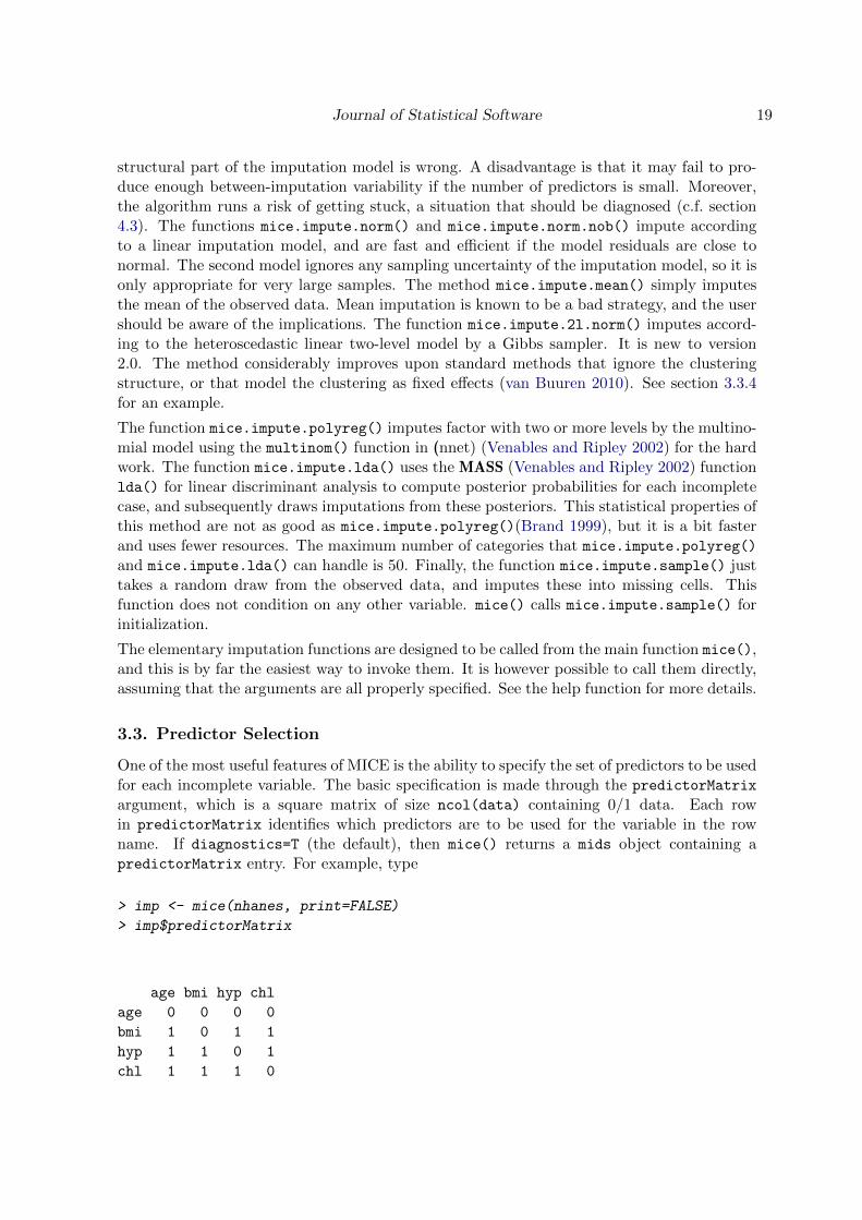
One of the most useful features of MICE is the ability to specify the set of predictors to be usedfor each incomplete variable. The basic specification is made through the predictorMatrix
argument, which is a square matrix of size ncol(data) containing 0/1 data. Each rowin predictorMatrix identifies which predictors are to be used for the variable in the rowname. If diagnostics=T (the default), then mice() returns a mids object containing apredictorMatrix entry. For example, type
> imp <- mice(nhanes, print=FALSE)
> imp$predictorMatrix
age bmi hyp chl
age 0 0 0 0
bmi 1 0 1 1
hyp 1 1 0 1
chl 1 1 1 0

20 MICE: Multivariate Imputation by Chained Equations
The row correspond to incomplete target variables, in the sequence as they appear in data.Row and column names of the predictorMatrix are ignored on input, and overwritten bymice() on output. A value of 1 indicates that the column variable is used as a predictorto impute the target (row) variable, and a 0 means that it is not used. Thus, in the aboveexample, bmi is predicted from age, hyp and chl. Note that the diagonal is 0 since a variablecannot predict itself. Since age contains no missing data, mice() silently sets all values inthe row to 0. The default setting of the predictorMatrix specifies that all variables predictall others.
Removing a predictor
The user can specify a custom predictorMatrix, thereby effectively regulating the number ofpredictors per variable. For example, suppose that bmi is considered irrelevant as a predictor.Setting all entries within the bmi column to zero effectively removes it from the predictor set,e.g.
> pred <- imp$predictorMatrix
> pred[,"bmi"] <- 0
> pred
age bmi hyp chl
age 0 0 0 0
bmi 1 0 1 1
hyp 1 0 0 1
chl 1 0 1 0
will not use bmi as a predictor, but still impute it. Using this new specification, we createimputations as
> imp <- mice(nhanes, pred=pred, pri=F)
This imputes the incomplete variables hyp and chl without using bmi as a predictor.
Skipping imputation
Suppose that we want to skip imputation of bmi, and leave it as it is. This can be achievedby 1) eliminating bmi from the predictor set, and 2) setting the imputation method to "".More specifically
> ini <- mice(nhanes2, maxit=0, pri=F)
> pred <- ini$pred
> pred[,"bmi"] <- 0
> meth <- ini$meth
> meth["bmi"] <- ""
> imp <- mice(nhanes2, meth=meth, pred=pred, pri=F)
> imp$imp$bmi

Journal of Statistical Software 21
1 2 3 4 5
1 NA NA NA NA NA
3 NA NA NA NA NA
4 NA NA NA NA NA
6 NA NA NA NA NA
10 NA NA NA NA NA
11 NA NA NA NA NA
12 NA NA NA NA NA
16 NA NA NA NA NA
21 NA NA NA NA NA
The first statement calls mice() with the maximum number of iterations maxit set to zero.This is a fast way to create the mids object called ini containing the default settings. Itis then easy to copy and edit the predictorMatrix and method arguments of the mice()
function. Now mice() will impute NA into the missing values of bmi. In effect, the originalbmi (with the missing values included) is copied into the multiply imputed data set. Thistechnique is not only useful for ”keeping all the data together”, but also opens up ways toperforms imputation by nested blocks of variables. For examples where this could be useful,see Shen (2000) and Rubin (2003).
Intercept imputation
Eliminating all predictors for bmi can be done by
> pred <- ini$pred
> pred["bmi",] <- 0
> imp <- mice(nhanes2, pred=pred, pri=F)
> imp$imp$bmi
1 2 3 4 5
1 22.0 27.5 29.6 27.4 33.2
3 22.0 28.7 21.7 21.7 35.3
4 28.7 29.6 27.5 20.4 33.2
6 20.4 24.9 30.1 30.1 30.1
10 27.5 20.4 22.5 26.3 25.5
11 20.4 35.3 33.2 22.0 35.3
12 28.7 25.5 27.2 22.0 29.6
16 20.4 30.1 24.9 26.3 35.3
21 22.0 35.3 21.7 24.9 25.5
Imputations for bmi are now sampled (by mice.impute.pmm()) under the intercept-onlymodel. Note that these imputations are appropriate only under the MCAR assumption.
Multilevel imputation
Imputation of multilevel data poses special problems. Most techniques have been developedunder the joint modeling perspective (Schafer and Yucel 2002; Yucel 2008; Goldstein et al.2009). Some work within the context of FCS has been done (Jacobusse 2005), but this is

22 MICE: Multivariate Imputation by Chained Equations
still an open research area. The mice package include the mice.impute.2l.norm() function,which can be used to impute missing data under a linear multilevel model. The functionwas contributed by Roel de Jong, and implements the Gibbs sampler for the linear multilevelmodel where the within-class error variance is allowed to vary (Kasim and Raudenbush 1998).Heterogeneity in the variances is essential for getting good imputations in multilevel data.The method is an improvement over simpler methods like flat-file imputation or per-groupimputation (van Buuren 2010).
Using mice.impute.2l.norm() deviates from other elementary imputation functions in MICEin two respects. It requires the specification of the fixed effects, the random effects andthe class variable. Furthermore, it assumes that the predictors contain a column of onesrepresenting the intercept. Random effects are coded in the predictor matrix as a ’2’. Theclass variable (only one is allowed) is coded by a ’-2’. The example below uses the popularitydata of (Hox 2002). The dependent variable is pupil popularity, which contains 848 missingvalues. There are two random effects: const (intercept) and sex (slope), one fixed effect(texp), and one class variable (school). Imputations can be generated as
> popmis[1:3,]
pupil school popular sex texp const teachpop
1 1 1 NA 1 24 1 7
2 2 1 NA 0 24 1 7
3 3 1 7 1 24 1 6
> ini <- mice(popmis, maxit=0)
> pred <- ini$pred
> pred["popular",] <- c(0, -2, 0, 2, 1, 2, 0)
> imp <- mice(popmis, meth=c("","","2l.norm","","","",""), pred=pred, maxit=1)
iter imp variable
1 1 popular
1 2 popular
1 3 popular
1 4 popular
1 5 popular
Warning message:
In check.data(data, predictorMatrix, method, nmis, nvar) :
Constant predictor(s) detected: const
The extension to the multivariate case will be obvious. The warning at the end is normalbehaviour.
Advice on predictor selection
The predictorMatrix argument is especially useful when dealing with data sets with a largenumber of variables. We now provide some advice regarding the selection of predictors forlarge data, especially with many incomplete data.

Journal of Statistical Software 23
As a general rule, using every bit of available information yields multiple imputations thathave minimal bias and maximal certainty.(Meng 1995; Collins et al. 2001) This principleimplies that the number of predictors in should be chosen as large as possible. Including asmany predictors as possible tends to make the MAR assumption more plausible, thus reducingthe need to make special adjustments for NMAR mechanisms.(Schafer 1997)
However, data sets often contain several hundreds of variables, all of which can potentiallybe used to generate imputations. It is not feasible (because of multicollinearity and computa-tional problems) to include all these variables. It is also not necessary. In our experience, theincrease in explained variance in linear regression is typically negligible after the best, say,15 variables have been included. For imputation purposes, it is expedient to select a suitablesubset of data that contains no more than 15 to 25 variables. van Buuren et al. (1999) providethe following strategy for selecting predictor variables from a large data base:
1. Include all variables that appear in the complete-data model, i.e., the model that willbe applied to the data after imputation. Failure to do so may bias the complete-data analysis, especially if the complete-data model contains strong predictive relations.Note that this step is somewhat counter-intuitive, as it may seem that imputationwould artificially strengthen the relations of the complete-data model, which is clearlyundesirable. If done properly however, this is not the case. On the contrary, notincluding the complete-data model variables will tend to bias the results towards zero.Note that interactions of scientific interest also need to be included into the imputationmodel.
2. In addition, include the variables that are related to the nonresponse. Factors thatare known to have influenced the occurrence of missing data (stratification, reasons fornonresponse) are to be included on substantive grounds. Others variables of interest arethose for which the distributions differ between the response and nonresponse groups.These can be found by inspecting their correlations with the response indicator of thevariable to be imputed. If the magnitude of this correlation exceeds a certain level, thenthe variable is included.
3. In addition, include variables that explain a considerable amount of variance. Suchpredictors help to reduce the uncertainty of the imputations. They are crudely identifiedby their correlation with the target variable.
4. Remove from the variables selected in steps 2 and 3 those variables that have toomany missing values within the subgroup of incomplete cases. A simple indicator is thepercentage of observed cases within this subgroup, the percentage of usable cases.
Most predictors used for imputation are incomplete themselves. In principle, one could applythe above modeling steps for each incomplete predictor in turn, but this may lead to a cascadeof auxiliary imputation problems. In doing so, one runs the risk that every variable needs to beincluded after all. In practice, there is often a small set of key variables, for which imputationsare needed, which suggests that steps 1 through 4 are to be performed for key variables only.This was the approach taken in van Buuren et al. (1999), but it may miss important predictorsof predictors. A safer and more efficient, though more laborious, strategy is to perform themodeling steps also for the predictors of predictors of key variables. This is done in Oudshoornet al. (1999). We expect that it is rarely necessary to go beyond predictors of predictors. At

24 MICE: Multivariate Imputation by Chained Equations
the terminal node, we can apply a simply method like mice.impute.sample() that does notneed any predictors for itself.
Quick predictor selection
Correlations for the strategy outlined above can be calculated with the standard functioncor(). For example,
> cor(nhanes, use="pairwise.complete.obs")
age bmi hyp chl
age 1.0000000 -0.37185348 0.50569587 0.5074613
bmi -0.3718535 1.00000000 0.05127959 0.3734585
hyp 0.5056959 0.05127959 1.00000000 0.4286139
chl 0.5074613 0.37345853 0.42861391 1.0000000
calculates Pearson correlations using all available cases in each pair of variables. Similarly,
> cor(y=nhanes, x=!is.na(nhanes), use="pairwise.complete.obs")
age bmi hyp chl
age NA NA NA NA
bmi 0.086007808 NA 0.1386750 0.05297781
hyp 0.008428696 NA NA 0.04527583
chl -0.040128618 -0.01226069 -0.1069901 NA
Warning message:
In cor(y = nhanes, x = !is.na(nhanes), use = "pairwise.complete.obs") :
the standard deviation is zero
calculates the mutual correlations between the data and the response indicators. The warningcan be safely ignored and is caused by the fact that age contains no missing data.
The proportion of usable cases measures how many cases with missing data on the targetvariable actually have observed values on the predictor. The proportion will be low if bothtarget and predictor are missing on the same cases. If so, the predictor contains only littleinformation to impute the target variable, and could be dropped from the model, especiallyif the bivariate relation is not primary scientific interest. The proportion of usable cases canbe calculated as
> p <- md.pairs(nhanes)
> p$mr/(p$mr+p$mm)
age bmi hyp chl
age NaN NaN NaN NaN
bmi 1 0.0 0.1111111 0.2222222
hyp 1 0.0 0.0000000 0.1250000
chl 1 0.3 0.3000000 0.0000000

Journal of Statistical Software 25
For imputing hyp only 1 out of 8 cases was observed in predictor chl. Thus, predictor chl
does not contain much information to impute hyp, despite the substantial correlation of 0.42.If the relation is of no further scientific interest, omitting predictor chl from the model toimpute hyp will only have a small effect. Note that proportion of usable cases is asymmetric.
MICE V2.0 contains a new function quickpred() that calculates these quantities, and com-bines them automatically in a predictorMatrix that can be used to call mice(). Thequickpred() function assumes that the correlation is a sensible measure for the data athand (e.g. order of factor levels should be reasonable). For example,
> quickpred(nhanes)
age bmi hyp chl
age 0 0 0 0
bmi 1 0 1 1
hyp 1 0 0 1
chl 1 1 1 0
yields a predictorMatrix for a model that includes all predictors with an absolute correlationwith the target or with the response indicator of at least 0.1 (the default value of the mincor
argument). Observe that the predictor matrix need not always be symmetric. In particular,bmi is not a predictor of hyp, but hyp is a predictor of bmi here. This can occur because thecorrelation of hyp with the response indicator of bmi (0.139) exceeds the threshold.
The quickpred() function has arguments that change the minimum correlation, that allowto select predictor based on their proportion of usable cases, and that can specify variablesthat should always be included or excluded. It is also possible to specify thresholds per targetvariable, or even per target-predictor combination. See the help files for more details.
It is easy to use the function in conjunction with mice(). For example,
> imp <- mice(nhanes, pred=quickpred(nhanes, minpuc=0.25, include="age"))
imputes the data from a model where the minimum proportion of usable cases is at least 0.25and that always includes age as a predictor.
Any interactions of interest need to be appended to the data before using quickpred(). Forlarge data, the user can experiment with the mincor, minpuc, include and exclude argu-ments to trim the imputation problem to a reasonable size. The application of quickpred()can substantially cut down the time needed to specify the imputation model for data withmany variables.
3.4. Passive Imputation
There is often a need for transformed, combined or recoded versions of the data. In thecase of incomplete data, one could impute the original, and transform the completed originalafterwards, or transform the incomplete original and impute the transformed version. If,however, both the original and the transform are needed within the imputation algorithm,neither of these approaches work because one cannot be sure that the transformation holdsbetween the imputed values of the original and transformed versions.

26 MICE: Multivariate Imputation by Chained Equations
MICE has a special mechanism, called passive imputation, to deal with such situations. Pas-sive imputation maintains the consistency among different transformations of the same data.The method can be used to ensure that the transform always depends on the most recentlygenerated imputations in the original untransformed data. Passive imputation is invoked byspecifying a ˜ (tilde) as the first character of the imputation method. The entire string,including the ˜ is interpreted as the formula argument in a call to model.frame(formula,
data[!r[,j],]). This provides a simple method for specifying a large variety of dependen-cies among the variables, such as transformed variables, recodes, interactions, sum scores, andso on, that may themselves be needed in other parts of the algorithm.
Preserving a transformation
As an example, suppose that previous research suggested that bmi is better imputed fromlog(chl) than from chl. We may thus want to add an extra column to the data withlog(chl), and impute bmi from log(chl). Any missing values in chl will also be presentin log(chl). The problem is to keep imputations in chl and log(chl) consistent with eachother, i.e. the imputations should respect their relationship. The following code will take careof this:
> nhanes2.ext <- cbind(nhanes2, lchl=log(nhanes2$chl))
> ini <- mice(nhanes2.ext, max=0, print=FALSE)
> meth <- ini$meth
> meth["lchl"] <- "˜log(chl)"
> pred <- ini$pred
> pred[c("hyp","chl"),"lchl"] <- 0
> pred["bmi","chl"] <- 0
> pred
age bmi hyp chl lchl
age 0 0 0 0 0
bmi 1 0 1 0 1
hyp 1 1 0 1 0
chl 1 1 1 0 0
lchl 1 1 1 1 0
> imp <- mice(nhanes2.ext, meth=meth, pred=pred)
> complete(imp)
...
age bmi hyp chl lchl
1 1 41.50753 2 229 5.433722
2 2 22.70000 1 187 5.231109
3 1 30.69074 1 187 5.231109
4 3 16.22606 1 199 5.293305
5 1 20.40000 1 113 4.727388
...

Journal of Statistical Software 27
We defined the predictor matrix such that either chl or log(chl) is a predictor, but notboth at the same time, primarily to avoid collinearity. Moreover, we do not want to predictchl from lchl. Doing so would immobilize the Gibbs sampler at the starting imputation. Itis thus important to set the entry pred["chl","lchl"] equal to zero to avoid this. Afterrunning mice() we find imputations for both chl and lchl that respect the relation.
Note: A slightly easier way to create nhanes2.ext is to specify
> nhanes2.ext <- cbind(nhanes2, lchl=NA)
followed by the same commands. This has the advantage that the transform needs to bespecified only once. Since all values in lchl are now treated as missing, the size of imp willgenerally become (much) larger however. The first method is generally more efficient, but thesecond is easier.
Index of two variables
The idea can be extended to two or more columns. This is useful to create derived variablesthat should remain synchronized. As an example, we consider imputation of body mass index(bmi), which is defined as weight divided by height*height. It is impossible to calculate bmiif either weight or height is missing. Consider the data boys in mice.
> md.pattern(boys[,c("hgt","wgt","bmi")])
wgt hgt bmi
727 1 1 1 0
17 1 0 0 2
1 0 1 0 2
3 0 0 0 3
4 20 21 45
Data on weight and height are missing for 4 and 20 cases, respectively, resulting in 21 casesfor which bmi could not be calculated. Using passive imputation, we can impute bmi fromheight and weight by means of the I() operator.
> ini <- mice(boys,max=0,print=FALSE)
> meth <- ini$meth
> meth["bmi"] <- "˜I(wgt/(hgt/100)ˆ2)"
> pred <- ini$pred
> pred[c("wgt","hgt","hc","reg"),"bmi"] <- 0
> pred[c("gen","phb","tv"),c("hgt","wgt","hc")] <- 0
> pred
age hgt wgt bmi hc gen phb tv reg
age 0 0 0 0 0 0 0 0 0
hgt 1 0 1 0 1 1 1 1 1
wgt 1 1 0 0 1 1 1 1 1
bmi 1 1 1 0 1 1 1 1 1

28 MICE: Multivariate Imputation by Chained Equations
hc 1 1 1 0 0 1 1 1 1
gen 1 0 0 1 0 0 1 1 1
phb 1 0 0 1 0 1 0 1 1
tv 1 0 0 1 0 1 1 0 1
reg 1 1 1 0 1 1 1 1 0
The predictor matrix prevents that hgt or wgt are imputed from bmi, and takes care thatthere are no cases where hgt, wgt and bmi are simultaneous predictors. Passive imputationoverrules the selection of variables specified in the predictorMatrix argument. Thus, inthe above case, we might have well set pred["bmi",] <- 0 and obtain identical results.Imputations can now be created by
> imp <- mice(boys, pred=pred, meth=meth, maxit=20)
> complete(imp)[is.na(boys$bmi),]
age hgt wgt bmi hc gen phb tv reg
103 0.087 58.0 4.54 13.49584 39.0 G1 P1 1 west
366 0.177 57.5 4.95 14.97164 40.4 G1 P1 1 west
1617 1.481 85.5 12.04 16.47002 47.5 G1 P1 1 north
...
Observe than the imputed values for bmi are consistent with (imputed) values of hgt and wgt.
Note: The values of bmi in the original data have been rounded to two decimals. If desired,one can get that also in the imputed values by setting
> meth["bmi"] <- "˜round(wgt/(hgt/100)ˆ2,dig=2)"
Sum scores
The sum score is undefined if one of the variables to be added is missing. We can use sumscores of imputed variables within the Gibbs sampling algorithm to economize on the numberof predictors. For example, suppose we create a summary maturation score of the pubertalmeasurements gen, phb and tv, and use that score to impute the other variables instead ofthe three original pubertal measurements. We can achieve that by
> ini <- mice(cbind(boys,mat=NA),max=0,print=FALSE)
> meth <- ini$meth
> meth["mat"] <- "˜I(as.integer(gen) + as.integer(phb) +
+ as.integer(cut(tv,breaks=c(0,3,6,10,15,20,25))))"
> meth["bmi"] <- "˜I(wgt/(hgt/100)ˆ2)"
> pred <- ini$pred
> pred[c("gen","phb","tv"),"mat"] <- 0
> pred[c("hgt","wgt","hc","reg"),c("gen","phb","tv")] <- 0
> pred[c("wgt","hgt","hc","reg"),"bmi"] <- 0
> pred[c("gen","phb","tv"),c("hgt","wgt","hc")] <- 0
> pred[c("bmi","mat"),] <- 0
> pred

Journal of Statistical Software 29
age hgt wgt bmi hc gen phb tv reg mat
age 0 0 0 0 0 0 0 0 0 0
hgt 1 0 1 0 1 0 0 0 1 1
wgt 1 1 0 0 1 0 0 0 1 1
bmi 0 0 0 0 0 0 0 0 0 0
hc 1 1 1 0 0 0 0 0 1 1
gen 1 0 0 1 0 0 1 1 1 0
phb 1 0 0 1 0 1 0 1 1 0
tv 1 0 0 1 0 1 1 0 1 0
reg 1 1 1 0 1 0 0 0 0 1
mat 0 0 0 0 0 0 0 0 0 0
The maturation score mat is composed of the sum of gen, phb and tv. Since the first two arefactors, we need the as.integer() function to get the internal numerical codes. Furthermore,we recoded tv into 6 ordered categories by calling the cut() function, and use the categorynumber to calculate the sum score. The predictor matrix is set up so that either the set of(gen,phb,tv) or mat are predictors, but never at the same time. The number of predictorsfor say, hgt, has now dropped from 8 to 5, but imputation still incorporates the main relationsof interest. Imputations can now be generated and plotted by
> imp <- mice(cbind(boys,mat=NA), pred=pred, meth=meth, maxit=20)
> col <- c("blue","red")[1+as.numeric(is.na(boys$gen) |
+ is.na(boys$phb)|is.na(boys$tv))]
> with(complete(imp,1), plot(age,mat,type="n",
+ ylab="Maturation sum score", xlab="Age (years)"))
> with(complete(imp,1),points(age,mat,col=col))
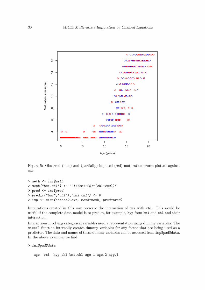
Figure 5 plots the derived maturation scores against age. Since no measurements were madebefore the age of 8 years, all scores on the left side are sums of three imputed values for gen,phb and tv. Note that imputation takes the form here of extreme extrapolation outside therange of the data. Some anomalies are present (two babies score a ’4’), but the overall patternis as expected.
Interaction terms
In some cases scientific interest focusses on interactions terms. For example, in experimentalstudies we may be interested in assessing whether the rate of change differs between twotreatment groups. In such cases, the primary goal is to get an unbiased estimate of the timeby group interaction. In general imputations should be conditional upon the interactionsof interest. However, interaction terms will be incomplete if the variables that make upthe interaction are incomplete. It is straightforward to solve this problem using passiveimputation.
Interactions between two continuous variables are often defined by subtracting the mean andtaking the product. In MICE we may say
> nhanes2.ext <- cbind(nhanes2, bmi.chl=NA)
> ini <- mice(nhanes2.ext, max=0, print=FALSE)
30 MICE: Multivariate Imputation by Chained Equations
0 5 10 15 20
46
810
1214
16
Age (years)
Mat
urat
ion
sum
sco
re
Figure 5: Observed (blue) and (partially) imputed (red) maturation scores plotted againstage.
> meth <- ini$meth
> meth["bmi.chl"] <- "˜I((bmi-25)*(chl-200))"
> pred <- ini$pred
> pred[c("bmi","chl"),"bmi.chl"] <- 0
> imp <- mice(nhanes2.ext, meth=meth, pred=pred)
Imputations created in this way preserve the interaction of bmi with chl. This would beuseful if the complete-data model is to predict, for example, hyp from bmi and chl and theirinteraction.
Interactions involving categorical variables need a representation using dummy variables. Themice() function internally creates dummy variables for any factor that are being used as apredictor. The data and names of these dummy variables can be accessed from imp$pad$data.In the above example, we find
> ini$pad$data
age bmi hyp chl bmi.chl age.1 age.2 hyp.1

Journal of Statistical Software 31
1 1 NA <NA> NA NA 0 0 NA
2 2 22.7 1 187 NA 1 0 0
3 1 NA 1 187 NA 0 0 0
4 3 NA <NA> NA NA 0 1 NA
5 1 20.4 1 113 NA 0 0 0
...
The factors age and hyp are internally represented by dummy variables age.1, age.2 andhyp.1. The interaction between age and bmi can be added as
> nhanes2.ext <- cbind(nhanes2,age.1.bmi=NA,age.2.bmi=NA)
> ini <- mice(nhanes2.ext, max=0, print=FALSE)
> meth <- ini$meth
> meth["age.1.bmi"] <- "˜I(age.1*(bmi-25))"
> meth["age.2.bmi"] <- "˜I(age.2*(bmi-25))"
> pred <- ini$pred
> pred[c("age","bmi"),c("age.1.bmi","age.2.bmi")] <- 0
> imp <- mice(nhanes2.ext, meth=meth, pred=pred, maxit=10)
Imputation of hyp and chl will now respect the interaction between age and bmi.
Squeeze
Imputed values that are implausible or impossible should not be accepted. For example,mice.impute.norm() can generate values outside the data range. Positive-valued variablescould occasionally receive negative values. For example, the following code produces a crash:
> nhanes2.ext <- cbind(nhanes2, lchl=NA)
> ini <- mice(nhanes2.ext,max=0,pri=FALSE)
> meth <- ini$meth
> meth[c("lchl","chl")] <- c("˜log(chl)","norm")
> pred <- ini$pred
> pred[c("hyp","chl"),"lchl"] <- 0
> pred["bmi","chl"] <- 0
> imp <- mice(nhanes2.ext, meth=meth, pred=pred, seed=1, maxit=10)
...
6 3 bmi hyp chl lchl
6 4 bmi hyp chl lchl
6 5 bmi hyp chl lchl
Error in `[<-.data.frame`(`*tmp*`, , i, value = list
(`log(chl)` = c(5.23110861685459, :
replacement element 1 has 24 rows, need 25
In addition: Warning message:
In log(chl) : NaNs produced
The problem here is that one of the imputed values in chl is negative. Negative values canoccur when imputing under the normal model, but leads here to a fatal error. One way to
32 MICE: Multivariate Imputation by Chained Equations
prevent this error is to squeeze the imputations into an allowable range. The squeeze()
function in MICE recodes any outlying values in the tail of the distribution to the nearestallowed value. Using meth["lchl"] <- "˜log(squeeze(chl, bounds=c(100,300)))" willsqueeze all imputed values into the range 100-300 before taking the log. This trick willsolve the problem, but does not store any squeezed values in chl, so lchl and chl becomeinconsistent. Depending on the situation, this may or may not be a problem. One way toensure consistency is to create an intermediate variable schl by passive imputation. Thus,schl contains the squeezed values, and takes over the role of chl within the algorithm. We’llsee an alternative in 3.5
Cautious remarks
There are some specific points that need attention when using passive imputation throughthe ˜ mechanism. Deterministic relations between columns remain only synchronized if thepassively imputed variable is updated immediately after any of its predictors are imputed. Soin the last example variables age.1.bmi and age.2.bmi should be updated each time after ageor bmi is imputed in order to stay synchronized. This can be done by changing the sequencein which the algorithm visits the columns. The mice() function does not automaticallychange the visiting sequence if passive variables are added. Section 3.6 provides techniquesfor setting the visiting sequence. Whether synchronization is really worthwhile will dependon the specific data at hand, but it is a healthy general strategy to pursue.
The ˜ mechanism may easily lead to highly correlated variables or linear dependencies amongpredictors. Sometimes we want this behavior on purpose, for example if we want to imputeusing both X and X2. However, linear dependencies among predictors will produce a fatalerror during imputation. In this section, our strategy has been to avoid this by requiring thateither the original or the passive variable can be a predictor. This strategy may not alwaysbe desired or feasible however.
Another point is that passive imputation may easily lock up the Gibbs sampler when it isnot done properly. Suppose that we make a copy bmi2 of bmi by passive imputation, andsubsequently use bmi2 to impute missing data in bmi. Re-imputing bmi from bmi2 will fixthe imputations to the starting imputations. This situation is easy to diagnose and correct(c.f. section 4.3).
The mice algorithm internally uses passive imputation to create dummy variables of factors.These dummy variables are created automatically and discarded within the main algorithm,and are always kept in sync with the original by passive imputation. The relevant data andsettings are stored within the list imp$pad. Normally, the user will not have to deal with this,but in case of running problems it could be useful to be aware of this. Section 4 providesmore details.
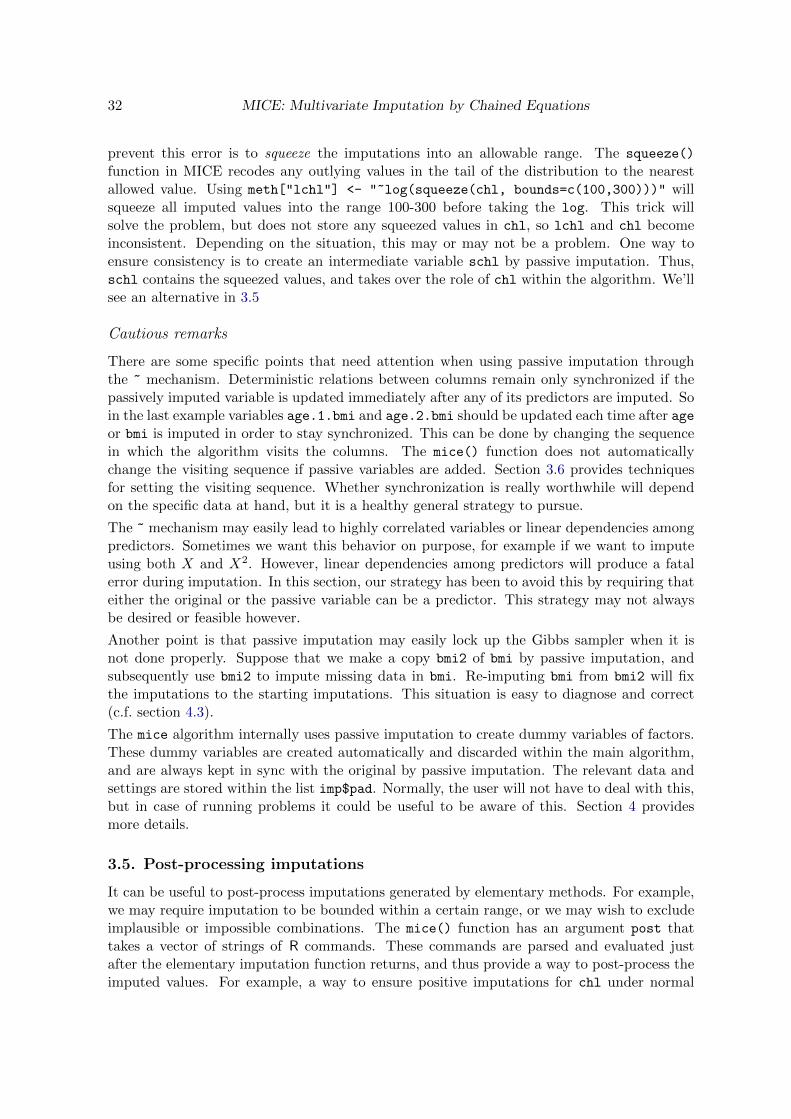
3.5. Post-processing imputations
It can be useful to post-process imputations generated by elementary methods. For example,we may require imputation to be bounded within a certain range, or we may wish to excludeimplausible or impossible combinations. The mice() function has an argument post thattakes a vector of strings of R commands. These commands are parsed and evaluated justafter the elementary imputation function returns, and thus provide a way to post-process theimputed values. For example, a way to ensure positive imputations for chl under normal
Journal of Statistical Software 33
imputation (c.f. section 3.4.5) is:
> nhanes2.ext <- cbind(nhanes2, lchl=NA)
> ini <- mice(nhanes2.ext,max=0,pri=FALSE)
> meth <- ini$meth
> meth[c("lchl","chl")] <- c("˜log(chl)","norm")
> pred <- ini$pred
> pred[c("hyp","chl"),"lchl"] <- 0
> pred["bmi","chl"] <- 0
> post <- ini$post
> post["chl"] <- "imp[[j]][,i] <- squeeze(imp[[j]][,i],c(100,300))"
> imp <- mice(nhanes2.ext, meth=meth, pred=pred, post=post, seed=1, maxit=10)
> imp$imp$chl
...
1 2 3 4 5
1 167.5031 100.0000 164.4944 246.3923 195.6364
4 159.0752 286.7699 295.2542 191.2493 184.1910
10 100.0000 255.7976 100.0000 180.3878 186.9328
11 109.5362 156.5706 148.7447 245.0541 100.0000
12 253.4219 190.5473 249.0979 232.9118 257.3956
15 143.2533 196.4840 203.3252 182.4529 156.7672
16 199.0560 100.0000 131.3612 116.2639 245.4151
20 147.4262 210.9002 249.6969 232.3344 258.4393
21 120.2079 156.9338 198.8863 195.5013 166.5104
24 241.8655 250.4261 240.6062 208.5305 300.0000
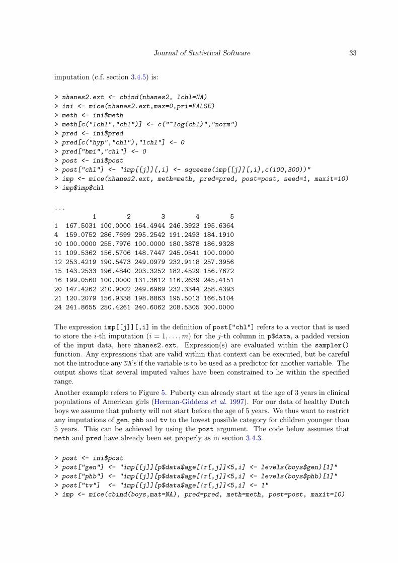
The expression imp[[j]][,i] in the definition of post["chl"] refers to a vector that is usedto store the i-th imputation (i = 1, . . . ,m) for the j-th column in p$data, a padded versionof the input data, here nhanes2.ext. Expression(s) are evaluated within the sampler()
function. Any expressions that are valid within that context can be executed, but be carefulnot the introduce any NA’s if the variable is to be used as a predictor for another variable. Theoutput shows that several imputed values have been constrained to lie within the specifiedrange.
Another example refers to Figure 5. Puberty can already start at the age of 3 years in clinicalpopulations of American girls (Herman-Giddens et al. 1997). For our data of healthy Dutchboys we assume that puberty will not start before the age of 5 years. We thus want to restrictany imputations of gen, phb and tv to the lowest possible category for children younger than5 years. This can be achieved by using the post argument. The code below assumes thatmeth and pred have already been set properly as in section 3.4.3.
> post <- ini$post
> post["gen"] <- "imp[[j]][p$data$age[!r[,j]]<5,i] <- levels(boys$gen)[1]"
> post["phb"] <- "imp[[j]][p$data$age[!r[,j]]<5,i] <- levels(boys$phb)[1]"
> post["tv"] <- "imp[[j]][p$data$age[!r[,j]]<5,i] <- 1"
> imp <- mice(cbind(boys,mat=NA), pred=pred, meth=meth, post=post, maxit=10)
34 MICE: Multivariate Imputation by Chained Equations
0 5 10 15 20
46
810
1214
16
Age (years)
Mat
urat
ion
sum
sco
re
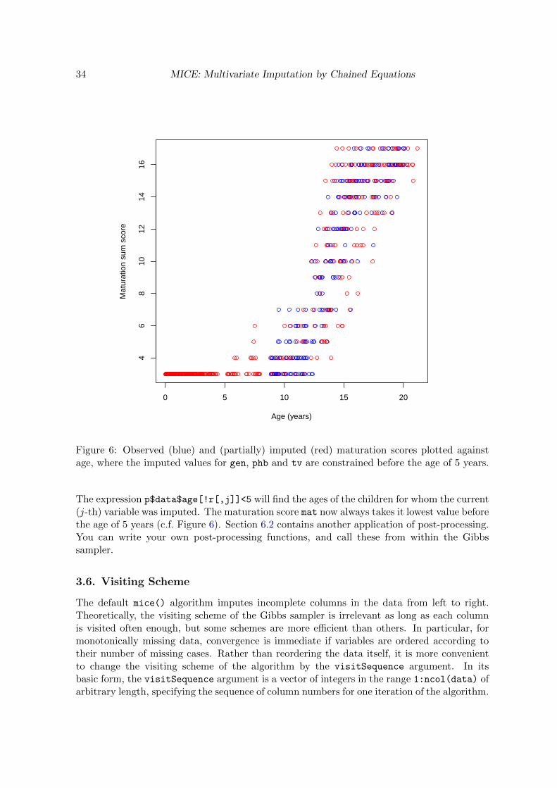
Figure 6: Observed (blue) and (partially) imputed (red) maturation scores plotted againstage, where the imputed values for gen, phb and tv are constrained before the age of 5 years.
The expression p$data$age[!r[,j]]<5 will find the ages of the children for whom the current(j-th) variable was imputed. The maturation score mat now always takes it lowest value beforethe age of 5 years (c.f. Figure 6). Section 6.2 contains another application of post-processing.You can write your own post-processing functions, and call these from within the Gibbssampler.
3.6. Visiting Scheme
The default mice() algorithm imputes incomplete columns in the data from left to right.Theoretically, the visiting scheme of the Gibbs sampler is irrelevant as long as each columnis visited often enough, but some schemes are more efficient than others. In particular, formonotonically missing data, convergence is immediate if variables are ordered according totheir number of missing cases. Rather than reordering the data itself, it is more convenientto change the visiting scheme of the algorithm by the visitSequence argument. In itsbasic form, the visitSequence argument is a vector of integers in the range 1:ncol(data) ofarbitrary length, specifying the sequence of column numbers for one iteration of the algorithm.

Journal of Statistical Software 35
Any given column may be visited more than once within the same iteration, which can beuseful to ensure proper synchronization among variables. It is mandatory that all columnswith missing data that are being used as predictors are visited, or else the function will stopwith an error.
As an example, rerun the code of section 3.4.4 to obtain imputed data imp that allow for theinteraction bmi.chl. The visiting scheme is
> imp$vis
bmi hyp chl bmi.chl
2 3 4 5
If visitSequence is not specified, the mice() function imputes the data from left to right. Inthis case, bmi.chl is calculated after chl is imputed, so at point bmi.chl is synchronized withboth bmi and chl. Note however that bmi.chl is not synchronized with bmi when imputinghyp, so bmi.chl is not representing the current interaction effect. This could result in wrongimputations. We can correct this by including an extra visit to bmi.chl after bmi has beenimputed:
> vis<-imp$vis
> vis<-append(vis,vis[4],1)
> vis
bmi bmi.chl hyp chl bmi.chl
2 5 3 4 5
> imp <- mice(nhanes2.ext, meth=meth, pred=pred, vis=vis)
iter imp variable
1 1 bmi bmi.chl hyp chl bmi.chl
1 2 bmi bmi.chl hyp chl bmi.chl
1 3 bmi bmi.chl hyp chl bmi.chl
...
The effect is that bmi.chl is now properly updated. By the way, a more efficient ordering ofthe variables is
> imp <- mice(nhanes2.ext, meth=meth, pred=pred, vis=c(2,4,5,3))
iter imp variable
1 1 bmi chl bmi.chl hyp
1 2 bmi chl bmi.chl hyp
1 3 bmi chl bmi.chl hyp
...
When the missing data pattern is close to monotone, convergence may be speeded by visitingthe columns in increasing order of the number of missing data. We can specify this order bythe "monotone" keyword as

36 MICE: Multivariate Imputation by Chained Equations
> imp <- mice(nhanes2.ext, meth=meth, pred=pred, vis="monotone")
iter imp variable
1 1 hyp bmi chl bmi.chl
1 2 hyp bmi chl bmi.chl
1 3 hyp bmi chl bmi.chl
...
4. Running MICE
4.1. Dry run
A dry run is a call to mice() with the maximum number of iterations maxit set to zero by
> ini <- mice(nhanes2, maxit=0)
A dry run is a fast way to create the mids object ini containing the default settings. Thedefault settings of the attributes of this mids object, like ini$method, ini$predictorMatrix,ini$post, and ini$visitSequence can be used to define user-specific settings. Especiallyfor datasets with many variables this is easier than defining these settings from scratch. Thistechnique was already used in many examples in section 3.
A mids object obtained with a dry run can also be used to include manually imputationsobtained from other software. It is essential that external imputations are stored in theproper format of the mids object. For example, the matrix import contains two imputationsfor nine missing values in bmi generated by other software. It can be assigned to the mids
object imp by
> import <- matrix(c(30,30,30,29,25,21,25,25,22,33,27,22,27,35,27,20,27,30),
+ byrow=T,nr=9)
> imp <- mice(nhanes)
> imp$imp$bmi[,1:2] <- import
> imp$imp$bmi
1 2 3 4 5
1 30 30 29.6 22.5 27.5
3 30 29 30.1 30.1 29.6
4 25 21 25.5 21.7 24.9
6 25 25 25.5 21.7 24.9
10 22 33 27.4 22.7 28.7
11 27 22 33.2 33.2 20.4
12 27 35 22.7 26.3 27.4
16 27 20 29.6 22.5 27.5
21 27 30 30.1 29.6 29.6

Journal of Statistical Software 37
It is important to realize that this technique assumes that the order of imputed values acrosssoftware systems is identical. Section 7 shows some alternative ways to interact with othersoftware.
The altered mids object can now be used as input for the Gibbs sampler by calling themice.mids function (see Section 4.2). Note that this requires all empty cells to be imputed,otherwise the sampler will get stuck on empty cells. Also, the altered mids object can be usedfor repeated complete data analyses by calling the with.mids function. For this use, emptycells in the imputation can be encoded by NA. The complete data method should then be ableto handle the missing data correctly.
4.2. Step by Step
The function mice.mids() takes a mids object as input, iterates maxit iterations and producesanother mids object as output. This function enables the user to split up the computations ofthe Gibbs sampler into smaller parts by providing a stopping point after every full iteration.There are various circumstances in which this might be useful:
� For large data, RAM memory may become exhausted if the number of iterations islarge. Returning to prompt/session level may alleviate these problems;
� The user wants to compute special convergence statistics at intermediate points, e.g.after each iteration, for monitoring convergence;
� For computing a ’few extra iterations’.
The imputation model itself is specified in the mice() function and cannot be changed withmice.mids (Well actually you can by tweaking the mids object directly, but this is not rec-ommended). The state of the random generator is saved with the mids object.
As a simple example, calculate two mids objects imp2 and imp as
> imp1 <- mice(nhanes, maxit=1, seed=612)
> a <- runif(10)
> imp2 <- mice.mids(imp1, maxit=3)
> imp <- mice(nhanes, maxit=4, seed=612)
Imputations in imp2 and imp are identical so all(imp2$imp$bmi==imp$imp$bmi) will yieldTRUE.
4.3. Assessing Convergence
There is no clear-cut method for determining whether the Gibbs sampling algorithm hasconverged. What is often done is to plot one or more parameters against the iteration number.The mice() function produces m parallel imputation streams. The mids object containscomponents chainMean and chainVar with the mean and variance of the imputations perstream, respectively. These can be plotted by the plot.mids object. On convergence, thedifferent streams should be freely intermingled with each other, without showing any definitetrends. Convergence is diagnosed when the variance between different sequences is no largerthan the variance with each individual sequence.
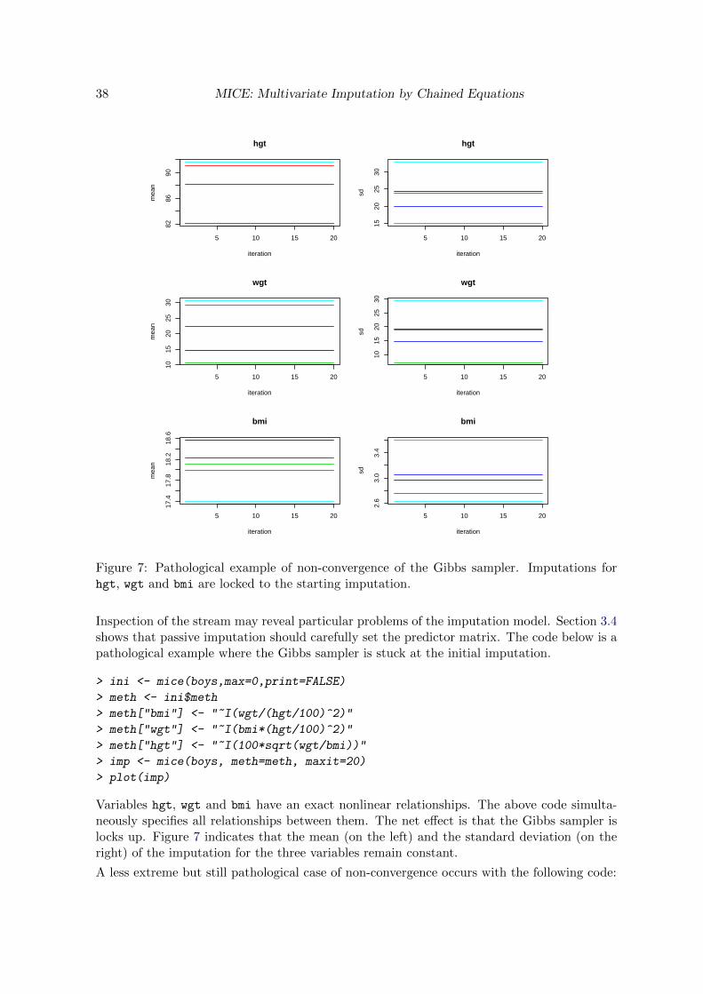
38 MICE: Multivariate Imputation by Chained Equations
5 10 15 20
8286
90
iteration
mea
nhgt
5 10 15 20
1520
2530
iteration
sd
hgt
5 10 15 20
1015
2025
30
iteration
mea
n
wgt
5 10 15 2010
1520
2530
iteration
sd
wgt
5 10 15 20
17.4
17.8
18.2
18.6
iteration
mea
n
bmi
5 10 15 20
2.6
3.0
3.4
iteration
sd
bmi
Figure 7: Pathological example of non-convergence of the Gibbs sampler. Imputations forhgt, wgt and bmi are locked to the starting imputation.
Inspection of the stream may reveal particular problems of the imputation model. Section 3.4shows that passive imputation should carefully set the predictor matrix. The code below is apathological example where the Gibbs sampler is stuck at the initial imputation.
> ini <- mice(boys,max=0,print=FALSE)
> meth <- ini$meth
> meth["bmi"] <- "˜I(wgt/(hgt/100)ˆ2)"
> meth["wgt"] <- "˜I(bmi*(hgt/100)ˆ2)"
> meth["hgt"] <- "˜I(100*sqrt(wgt/bmi))"
> imp <- mice(boys, meth=meth, maxit=20)
> plot(imp)
Variables hgt, wgt and bmi have an exact nonlinear relationships. The above code simulta-neously specifies all relationships between them. The net effect is that the Gibbs sampler islocks up. Figure 7 indicates that the mean (on the left) and the standard deviation (on theright) of the imputation for the three variables remain constant.
A less extreme but still pathological case of non-convergence occurs with the following code:
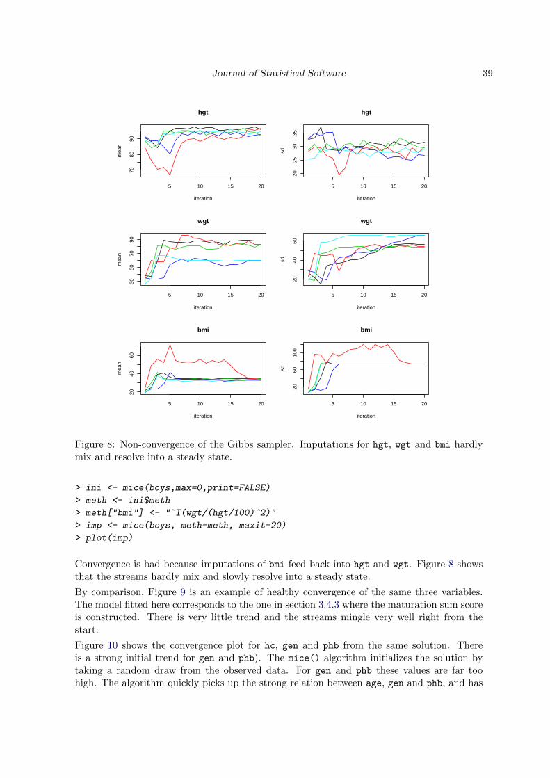
Journal of Statistical Software 39
5 10 15 20
7080
90
iteration
mea
nhgt
5 10 15 20
2025
3035
iteration
sd
hgt
5 10 15 20
3050
7090
iteration
mea
n
wgt
5 10 15 2020
4060
iteration
sd
wgt
5 10 15 20
2040
60
iteration
mea
n
bmi
5 10 15 20
2060
100
iteration
sd
bmi
Figure 8: Non-convergence of the Gibbs sampler. Imputations for hgt, wgt and bmi hardlymix and resolve into a steady state.
> ini <- mice(boys,max=0,print=FALSE)
> meth <- ini$meth
> meth["bmi"] <- "˜I(wgt/(hgt/100)ˆ2)"
> imp <- mice(boys, meth=meth, maxit=20)
> plot(imp)
Convergence is bad because imputations of bmi feed back into hgt and wgt. Figure 8 showsthat the streams hardly mix and slowly resolve into a steady state.
By comparison, Figure 9 is an example of healthy convergence of the same three variables.The model fitted here corresponds to the one in section 3.4.3 where the maturation sum scoreis constructed. There is very little trend and the streams mingle very well right from thestart.
Figure 10 shows the convergence plot for hc, gen and phb from the same solution. Thereis a strong initial trend for gen and phb). The mice() algorithm initializes the solution bytaking a random draw from the observed data. For gen and phb these values are far toohigh. The algorithm quickly picks up the strong relation between age, gen and phb, and has
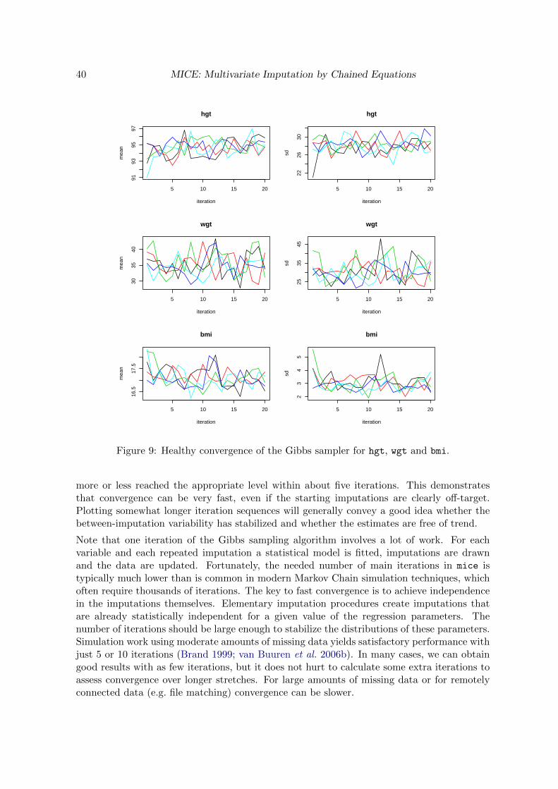
40 MICE: Multivariate Imputation by Chained Equations
5 10 15 20
9193
9597
iteration
mea
nhgt
5 10 15 20
2226
30
iteration
sd
hgt
5 10 15 20
3035
40
iteration
mea
n
wgt
5 10 15 2025
3545
iteration
sd
wgt
5 10 15 20
16.5
17.5
iteration
mea
n
bmi
5 10 15 20
23
45
iteration
sd
bmi
Figure 9: Healthy convergence of the Gibbs sampler for hgt, wgt and bmi.
more or less reached the appropriate level within about five iterations. This demonstratesthat convergence can be very fast, even if the starting imputations are clearly off-target.Plotting somewhat longer iteration sequences will generally convey a good idea whether thebetween-imputation variability has stabilized and whether the estimates are free of trend.
Note that one iteration of the Gibbs sampling algorithm involves a lot of work. For eachvariable and each repeated imputation a statistical model is fitted, imputations are drawnand the data are updated. Fortunately, the needed number of main iterations in mice istypically much lower than is common in modern Markov Chain simulation techniques, whichoften require thousands of iterations. The key to fast convergence is to achieve independencein the imputations themselves. Elementary imputation procedures create imputations thatare already statistically independent for a given value of the regression parameters. Thenumber of iterations should be large enough to stabilize the distributions of these parameters.Simulation work using moderate amounts of missing data yields satisfactory performance withjust 5 or 10 iterations (Brand 1999; van Buuren et al. 2006b). In many cases, we can obtaingood results with as few iterations, but it does not hurt to calculate some extra iterations toassess convergence over longer stretches. For large amounts of missing data or for remotelyconnected data (e.g. file matching) convergence can be slower.
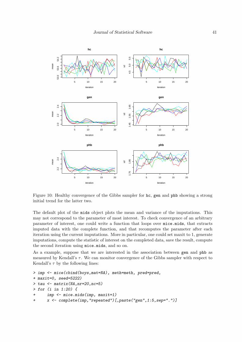
Journal of Statistical Software 41
5 10 15 20
53.0
53.6
54.2
iteration
mea
nhc
5 10 15 20
4.5
5.0
5.5
iteration
sd
hc
5 10 15 20
2.0
2.2
2.4
iteration
mea
n
gen
5 10 15 201.
451.
551.
65
iteration
sd
gen
5 10 15 20
2.2
2.4
iteration
mea
n
phb
5 10 15 20
1.75
1.85
iteration
sd
phb
Figure 10: Healthy convergence of the Gibbs sampler for hc, gen and phb showing a stronginitial trend for the latter two.
The default plot of the mids object plots the mean and variance of the imputations. Thismay not correspond to the parameter of most interest. To check convergence of an arbitraryparameter of interest, one could write a function that loops over mice.mids, that extractsimputed data with the complete function, and that recomputes the parameter after eachiteration using the current imputations. More in particular, one could set maxit to 1, generateimputations, compute the statistic of interest on the completed data, save the result, computethe second iteration using mice.mids, and so on.
As a example, suppose that we are interested in the association between gen and phb asmeasured by Kendall’s � . We can monitor convergence of the Gibbs sampler with respect toKendall’s � by the following lines:
> imp <- mice(cbind(boys,mat=NA), meth=meth, pred=pred,
+ maxit=0, seed=5222)
> tau <- matrix(NA,nr=20,nc=5)
> for (i in 1:20) {
+ imp <- mice.mids(imp, maxit=1)
+ x <- complete(imp,"repeated")[,paste("gen",1:5,sep=".")]
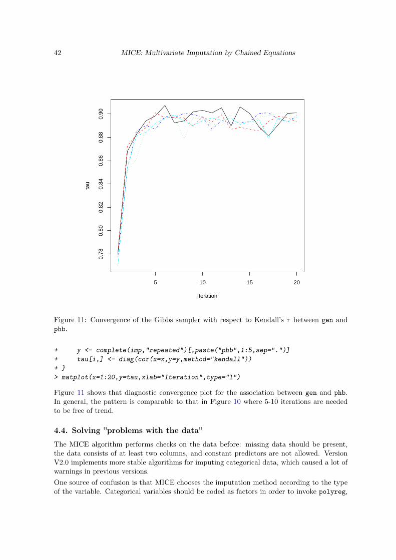
42 MICE: Multivariate Imputation by Chained Equations
5 10 15 20
0.78
0.80
0.82
0.84
0.86
0.88
0.90
Iteration
tau
Figure 11: Convergence of the Gibbs sampler with respect to Kendall’s � between gen andphb.
+ y <- complete(imp,"repeated")[,paste("phb",1:5,sep=".")]
+ tau[i,] <- diag(cor(x=x,y=y,method="kendall"))
+ }
> matplot(x=1:20,y=tau,xlab="Iteration",type="l")
Figure 11 shows that diagnostic convergence plot for the association between gen and phb.In general, the pattern is comparable to that in Figure 10 where 5-10 iterations are neededto be free of trend.
4.4. Solving ”problems with the data”
The MICE algorithm performs checks on the data before: missing data should be present,the data consists of at least two columns, and constant predictors are not allowed. VersionV2.0 implements more stable algorithms for imputing categorical data, which caused a lot ofwarnings in previous versions.
One source of confusion is that MICE chooses the imputation method according to the typeof the variable. Categorical variables should be coded as factors in order to invoke polyreg,

Journal of Statistical Software 43
otherwise pmm will be selected. Variables with many categories (>20) are often problematic.Internally, MICE will create a dummy variable for each category, which can produce very largematrices, time consuming calculations, introduce empty cell problems and cause instabilityproblems of the algorithm. For variable with many categories, we therefore recommend pmm.
The mice function was programmed for flexibility, and not to minimize the use of time orresources. Combined with the greedy nature of R in general and the fact that the methoddoes not use compiled functions, this poses some limits to the size of the data sets and thetype of data that can be analyzed. The time that mice needs depends primarily on the choiceof the elementary imputation methods. Methods like pmm and norm are fast, while others,logreg and polyreg, can be slow. If there are many categorical variables, each with manycategories, one can speed up the algorithm considerably by imputing (some of the) variablesas numerical variables with pmm instead of polyreg. Since pmm imputes only values that areobserved, the original categories of the variable are preserved.
A frequent source of problems is caused by predictors that are (almost) linearly related. For ex-ample, if one predictor can be written as a linear combination of some others, then this resultsin messages like ’Error in Solve.default(t(xobs) %*% xobs) : system is computa-
tionally singular: reciprocal condition number = 2.87491e-20’ or ’Error in sol-
ve.default(t(xobs) %*% xobs) : Lapack routine dgesv: system is exactly singular.’
The solution to collinearity is to eliminate duplicate information, for example by specifyinga reduced set of predictors via the predictorMatrix argument. Sometimes the source of theproblem is obvious, for example if there are sum scores. However, finding the sets of nearlydependent variables can prove to be difficult and laborious. One trick that we use in practiceis to study the last eigenvector of the covariance matrix of the incomplete data (after listwisedeletion). Variables with high values on that factor often cause the problems. Alternatively,one could revert to collinearity diagnostics like the VIF (Kleinbaum et al. (1988)) or graphicaldisplays (Cook and Weisberg (1999)). Pedhazur (Pedhazur (1973)) provides a good discus-sion on multicollinearity. There is certainly room for improvement here. The ambitious usermight like to write elementary imputation functions that are less sensitive to collinearity, forexample, based on ridge regression or penalized splines.
If all fails, use the debugger. Functions in mice are all full R. This allows you to trace everydetail of your calculations, and eventually track down the source of the problem. This is yourlast resort, and requires you to understand our code, which can be difficult at times, even forus. Use traceback() to find out what R was doing at the time the error occurred. In orderto use the debugger set options(error = dump.frames) before the error occurs, and thentype debugger(). This will get you to choose the local frame where the error, and inspectthe current value of local variables. If you have suggestions for improvement, please let usknow.
4.5. Checking your Imputations
Once the algorithm has converged, it is important to inspect the imputations. In general, agood imputed value is a value that could have been observed had it not been missing. In thisphase, it is often useful to report results to the investigator who understands the science behindthe data. Since there are some many aspects that we could look at, we have refrained fromimplemented specific tools. It is however not difficult with the powerful graphical functions inlattice() to make diagnostic plots for checking the imputations. We will give some examples

44 MICE: Multivariate Imputation by Chained Equations
below, following the ideas of Raghunathan and Bondarenko (2007).
The MAR assumption can never be tested from the observed data. One can however checkwhether the imputations created by mice() are plausible. As a first step one can plot densitiesof both the observed and imputed values of all variables to see whether the imputations arereasonable. Differences in the densities between the observed and imputed values may suggesta problem that needs to be further checked. The densityplot() function from the latticepackage contains can be used to create such a plot as follows:
> library(lattice)
> long <- complete(imp,"long")
> levels(long$.imp) <- paste("Imputation",1:5)
> long <- cbind(long, hc.na=is.na(imp$data$hc))
> densityplot(˜hc|.imp, data=long, group=hc.na, plot.points=FALSE,
+ ref=TRUE, xlab="Head circumference",scales=list(y=list(draw=F)),
+ par.settings=simpleTheme(col.line=rep(c("blue","red"))),
+ auto.key = list(columns=2,text=c("Observed","Imputed")))
Figure 12 shows that the imputed values are higher than the observed values. The reasonis that the probability that hc (head circumference) is missing is larger for older boys. Ingeneral, plots like this are useful to detect interesting differences between the observed andimputed data.
Another diagnostic tool involves comparing the distributions of observed and imputed dataconditional on the propensity score.(Raghunathan and Bondarenko 2007) The idea is thatthe conditional distributions should be similar if the assumed model for creating multipleimputations is a good fit. The following statements assume that the missing data indicatorhc.na for hc is also part of the imp.
> fit.hc <- with(imp, glm(hc.na˜age+wgt+hgt+mat+reg,family=binomial))
> ps <- rowMeans(sapply(fit.hc$analyses, fitted.values))
> hc.1 <- complete(imp,1)$hc
> hc.na <- is.na(imp$data$hc)
> xyplot(hc.1 ˜ ps, groups=hc.na,
+ xlab="Probability of missing head circumference",
+ ylab="Head circumference",
+ par.settings = simpleTheme(col.points = rep(c("blue","red")),
+ cex=1.2, pch=19),
+ auto.key = list(columns=2, text = c("Observed","Imputed")))
Figure 13 plots head circumference (observed and imputed) against the propensity score,where the propensity score is equal to the average over the imputations. By definition, thereare more imputed values on the right hand side of the display than on the left hand side.The striped pattern in the distribution of the propensity score is related to region (variablereg). More missing data appear in the city and in the western part of the country. If theimputation model fits well, we expect that for a given propensity score, the distribution ofthe observed and imputed data conform well. This appears to be the case here, so this plotprovides evidence that the imputations are good. Realize however that the comparison is
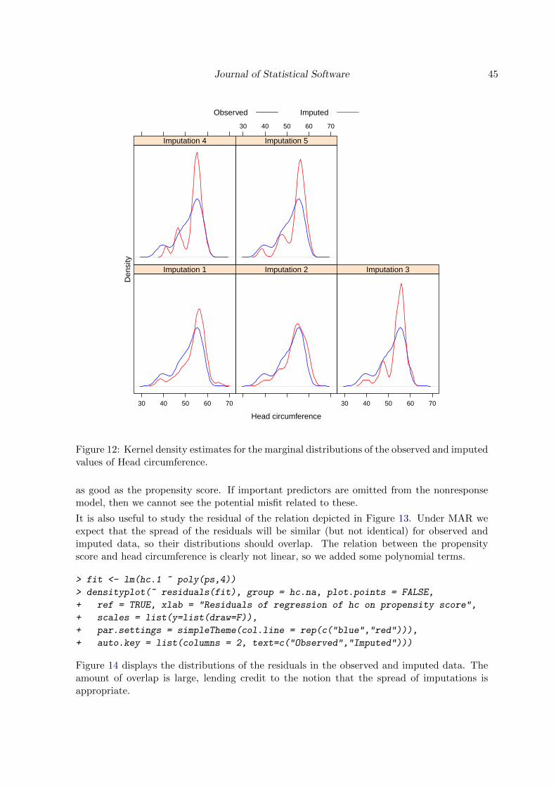
Journal of Statistical Software 45
Head circumference
Den
sity
30 40 50 60 70
Imputation 1 Imputation 2
30 40 50 60 70
Imputation 3
Imputation 4
30 40 50 60 70
Imputation 5
Observed Imputed
Figure 12: Kernel density estimates for the marginal distributions of the observed and imputedvalues of Head circumference.
as good as the propensity score. If important predictors are omitted from the nonresponsemodel, then we cannot see the potential misfit related to these.
It is also useful to study the residual of the relation depicted in Figure 13. Under MAR weexpect that the spread of the residuals will be similar (but not identical) for observed andimputed data, so their distributions should overlap. The relation between the propensityscore and head circumference is clearly not linear, so we added some polynomial terms.
> fit <- lm(hc.1 ˜ poly(ps,4))
> densityplot(˜ residuals(fit), group = hc.na, plot.points = FALSE,
+ ref = TRUE, xlab = "Residuals of regression of hc on propensity score",
+ scales = list(y=list(draw=F)),
+ par.settings = simpleTheme(col.line = rep(c("blue","red"))),
+ auto.key = list(columns = 2, text=c("Observed","Imputed")))
Figure 14 displays the distributions of the residuals in the observed and imputed data. Theamount of overlap is large, lending credit to the notion that the spread of imputations isappropriate.
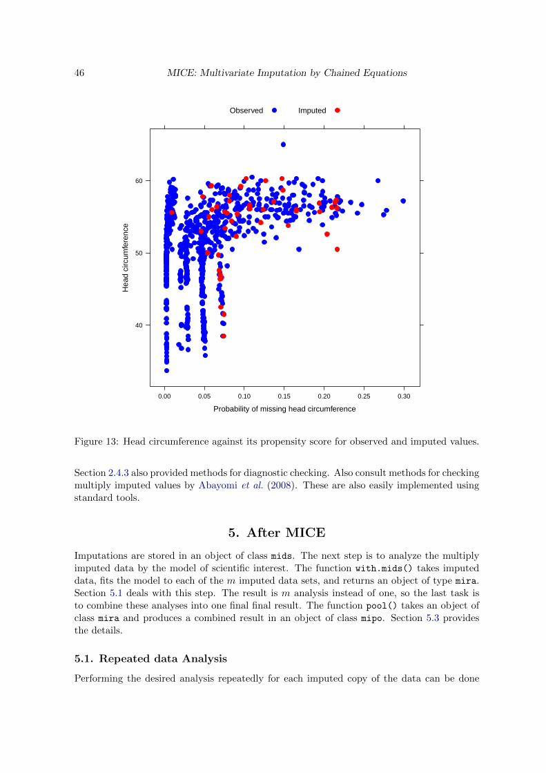
46 MICE: Multivariate Imputation by Chained Equations
Probability of missing head circumference
Hea
d ci
rcum
fere
nce
40
50
60
0.00 0.05 0.10 0.15 0.20 0.25 0.30
Observed Imputed
Figure 13: Head circumference against its propensity score for observed and imputed values.
Section 2.4.3 also provided methods for diagnostic checking. Also consult methods for checkingmultiply imputed values by Abayomi et al. (2008). These are also easily implemented usingstandard tools.
5. After MICE
Imputations are stored in an object of class mids. The next step is to analyze the multiplyimputed data by the model of scientific interest. The function with.mids() takes imputeddata, fits the model to each of the m imputed data sets, and returns an object of type mira.Section 5.1 deals with this step. The result is m analysis instead of one, so the last task isto combine these analyses into one final final result. The function pool() takes an object ofclass mira and produces a combined result in an object of class mipo. Section 5.3 providesthe details.
5.1. Repeated data Analysis
Performing the desired analysis repeatedly for each imputed copy of the data can be done
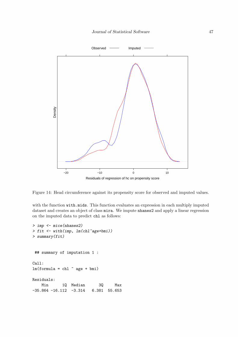
Journal of Statistical Software 47
Residuals of regression of hc on propensity score
Den
sity
−20 −10 0 10
Observed Imputed
Figure 14: Head circumference against its propensity score for observed and imputed values.
with the function with.mids. This function evaluates an expression in each multiply imputeddataset and creates an object of class mira. We impute nhanes2 and apply a linear regressionon the imputed data to predict chl as follows:
> imp <- mice(nhanes2)
> fit <- with(imp, lm(chl˜age+bmi))
> summary(fit)
## summary of imputation 1 :
Call:
lm(formula = chl ˜ age + bmi)
Residuals:
Min 1Q Median 3Q Max
-35.864 -16.112 -3.314 6.381 55.653
48 MICE: Multivariate Imputation by Chained Equations
Coefficients:
Estimate Std. Error t value Pr(>|t|)
(Intercept) -13.269 42.865 -0.310 0.759957
age2 54.892 14.159 3.877 0.000872 ***
age3 63.448 15.316 4.143 0.000462 ***
bmi 6.550 1.466 4.468 0.000212 ***
---
Residual standard error: 27.96 on 21 degrees of freedom
Multiple R-squared: 0.5829, Adjusted R-squared: 0.5233
F-statistic: 9.782 on 3 and 21 DF, p-value: 0.0003065
## summary of imputation 2 :
Call:
lm(formula = chl ˜ age + bmi)
...
We can access the results of the third imputation by fit$ana[[3]]. The with.mids()
function accepts any valid expression. For example, to calculate the contingency table ofoverweight by age per imputation, we can use the following:
> expr <- expression(ov<-cut(bmi,c(10,25,50)),table(age,ov))
> fit <- with(imp, eval(expr))
> fit$an
[[1]]
ov
age (10,25] (25,50]
1 3 9
2 3 4
3 4 2
[[2]]
ov
age (10,25] (25,50]
1 4 8
2 2 5
3 4 2
...
The function with.mids replaces lm.mids and glm.mids. For compatibility reasons, thelatter two functions remain available.
5.2. Extracting imputed data

Journal of Statistical Software 49
An alternative is to export the imputed data into a conventional rectangular form, followedby the analysis of the imputed data. The complete() function extracts imputed data setsfrom a mids object, and returns the completed data as a data frame. For example,
> com <- complete(imp, 3)
extracts the third complete data set from a multiply imputed data in imp. Specifying
> com <- complete(imp, "long")
produces a long matrix com where the m completed data matrices are vertically stacked andpadded with the imputation number in a column called .imp. This form is convenient formaking point estimates and for exporting multiply imputed data to other software. Otheroptions are broad and repeated, which produce complete data in formats that are convenientfor investigating between-imputation patterns. One could also optionally include the originalincomplete data.
An alternative way of creating the above contingency tables using complete() is:
> com <- complete(imp, "long", include=TRUE)
> by(cbind(age=com$age,ov=cut(com$bmi,c(10,25,50))), com$.imp, table)
INDICES: observed
ov
age 1 2
1 2 5
2 2 3
3 2 2
---------------------------------------
INDICES: 1
ov
age 1 2
1 3 9
2 3 4
3 4 2
---------------------------------------
INDICES: 2
ov
age 1 2
1 4 8
2 2 5
3 4 2
...
5.3. Pooling
Rubin (1987) developed a set of rules for combining the separate estimates and standarderrors from each of the m imputed datasets into an overall estimate with standard error,

50 MICE: Multivariate Imputation by Chained Equations
confidence intervals and P -values. These rules are based on asymptotic theory on the normaldistribution, and are implemented in the functions pool() and pool.scalar().
mira objects
The function pool() take an object of class mira and creates an object of class mipo (multipleimputed pooled outcomes). For example,
> fit <- with(imp, lm(chl˜age+bmi))
> est <- pool(fit)
> est
Call: pool(object = fit)
Pooled coefficients:
(Intercept) age2 age3 bmi
-34.719650 50.667652 66.633077 7.265418
Fraction of information about the coefficients missing due to nonresponse:
(Intercept) age2 age3 bmi
0.14285402 0.23395614 0.04554637 0.14242471
More detailed output can be obtained by summary(pool(fit)).
The function pool() works for any object having both coef() and vcov() methods. Thefunction tests for this, and aborts if it fails to find an appropriate method. A list of methodsfor which coef() and vcov() exists can be obtained by
> methods(coef)
> methods(vcov)
[1] coef.aov* coef.Arima* coef.default* coef.fitdistr*
coef.lda* coef.listof* coef.loglm* coef.multinom*
coef.nls* coef.nnet* coef.ridgelm*
Non-visible functions are asterisked
[1] vcov.Arima* vcov.glm* vcov.lm* vcov.mlm*
vcov.multinom* vcov.negbin* vcov.nls* vcov.polr*
vcov.rlm*
Non-visible functions are asterisked
In addition, the pool() function will also work for objects of class lme defined in the packagenlme. It is possible to pool the fixed coefficients from a linear mixed model according toRubin’s rules. By default the number of degrees of freedom is calculated using the method ofBarnard and Rubin (1999).
Scalars
The function pool.scalar pools univariate estimates of m repeated complete data analysisaccording to Rubin’s rules. The arguments of the function are two vectors containing the m

Journal of Statistical Software 51
repeated complete data estimates and their corresponding m variances. The function returnsa list containing the pooled estimate, the between, within and total variance, the relativeincrease in variance due to nonresponse, the degrees of freedom for the t reference distributionand the fraction of missing information due to nonresponse. This function is useful when theestimated parameters are not obtained through one of the regular R modeling functions.
Explained variance R2
For combining estimates of R2 and adjusted R2 one can use the function pool.r.squared.The method is based on the familiar Fisher z transformation for correlations. Its propertiesin the context of multiple imputation were studied by Harel (2009).
Model testing
The function pool.compare() compares two nested models fitted on multiply imputed data.The function implements the Wald test and the likelihood ratio test. The function can be usedto test whether one or more variables should be present in the complete-data model. Variableselection in the context of multiple imputation is somewhat different. Several strategieshave been proposed that count the number of times that variable is in the model (Brand1999; Heymans et al. 2007; Wood et al. 2008). The pool.compare() function provides analternative that takes the between-imputation variability into account.
The Wald test can be used when the completed-data estimates and their covariance matricesare known (e.g. for estimates obtained with lm), and when the dimensionality of the estimatesis not too high. The pool.compare() function with the argument method="Wald" pools theP -values for comparing the nested models using the method of Li et al. (1991).
> imp <- mice(nhanes2, pri=F)
> fit0 <- with(data=imp,expr=lm(bmi˜age+hyp))
> fit1 <- with(data=imp,expr=lm(bmi˜age+hyp+chl))
> stat <- pool.compare(fit1, fit0, method="Wald")
> stat$p
[,1]
[1,] 0.004167355
Meng and Rubin (1992) provide a procedure for testing nested hypotheses by likelihood ratiotests from multiple imputed data. The likelihood function needs to be fully specified inorder to calculate the likelihood ratio statistics at the average over the imputations of theparameter estimates under both the null and alternative hypotheses. The current version ofpool.compare() implements the likelihood function for logistic regression, i.e. complete-datamodels obtained with glm(family="binomial"). The example below illustrates the use ofthe method in the boys data. The question is whether the factor reg (region, with five levels)should be included in the logistic regression model for onset of puberty.
> imp <- mice(boys, pri=F)
> fit0 <- with(data=imp, expr=glm(I(gen>levels(gen)[1])˜hgt+hc,
+ family=binomial))
> fit1 <- with(data=imp, expr=glm(I(gen>levels(gen)[1])˜hgt+hc+reg,
52 MICE: Multivariate Imputation by Chained Equations
+ family=binomial))
> stat <- pool.compare(fit1, fit0, method="likelihood", data=imp)
> stat$p
> stat$p
[1] 9.740416e-06
The difference as measured by the likelihood ratio statistic is highly significant, which providesfirm evidence that reg should indeed be included.
6. Miscellaneous topics
6.1. Adding your own Imputation Functions
Some organizations have made considerable investments to develop procedures for imputingkey variables, like income or family size, whose values are subject to all kinds of subtleconstraints. Using one of the built-in imputation methods could be a waste of this investment,and may fail to produce what is needed.
It is possible to write your own elementary imputation function, and call this function fromwithin the Gibbs sampling algorithm. The easiest way to write such a function is to copy andmodify an existing mice.impute.xxx() function, for example mice.impute.norm(). Mostelementary imputation functions have just three arguments: the variable to be imputed y,the response indicator ry and the matrix of predictors x (without intercept). The func-tion should return a vector of length(y)-sum(ry) imputations of the correct type. Consultmice.impute.norm() or mice.impute.polyreg() for inspiration. Your new function can becalled from within the Gibbs sampler by the method argument. For example, calling yourfunction mice.impute.myfunc() for each column can be done by typing
> mice(nhanes, method="myfunc")
Using this procedure enables you to speed up the algorithm by including pre-compiled Fortranor C code, or to dump imputation models for closer inspection.
6.2. Sensitivity analysis under MNAR
A common misunderstanding about multiple imputation is that it is restricted to MAR.While it is certainly true that imputation techniques commonly assume MAR, the theoryof multiple imputation is completely general and also applies to MNAR. Under MNAR, themodel fitted to the complete cases is incorrect for the missing cases, and thus cannot be usedfor imputation. Unless we have external data, there is no way of estimating the amount oferror.
A sensible alternative is to set up a number of plausible scenarios, and investigate the conse-quences of each of them on the final inferences. Chapter 6 in Rubin (1987) contains a numberof basic techniques. Up-to-date overviews of specialized MNAR models can be found in Little(2009b) and Albert and Follmann (2009). If the influence under these scenarios is small, thenthe analysis is said to be robust against the investigated violations of the MAR mechanism.

Journal of Statistical Software 53
Suppose that we have reason to believe that our imputations made under the MAR assumptionare too low, even after accounting for the predictive information in the available data. Onesimple trick is to multiply the imputations by a factor. In mice(), this is easily achievedby post-processing imputations through the post argument. The scenario involves increasingimputations for chl by 0% (MAR), 10%, 20%, 30%, 40% and 50% (MNAR).
> ini <- mice(nhanes2,max=0,pri=FALSE)
> post <- ini$post
> k <- seq(1,1.5,0.1)
> est <- vector("list",length(k))
> for (i in 1:length(k)) {
+ post["chl"] <- paste("imp[[j]][,i] <-",k[i],"* imp[[j]][,i]")
+ imp <- mice(nhanes2, post=post, seed=10, maxit=20)
+ fit <- with(imp, lm(bmi˜age+chl))
+ est[[i]] <- summary(pool(fit))
}
The parameters of interest under these six scenarios are stored in the list est. Inspection ofthese solutions reveals that the size of k primarily increases the intercept term. There is aslightly trend that moves the model estimates towards zero if k goes up. Note that we usedfixed seed value, so all differences between scenarios are strictly due to k.
Carefully monitor convergence if variables are highly correlated. A higher imputed value inchl will produce a higher than average imputation in bmi and hyp. If relations are strong,these higher average will feedback into a higher imputations for chl, which is then multipliedby k, and so on. Such feedback could result in explosive behavior of the Gibbs sampler thatshould be diagnosed and prevented. A remedy is to remove the strongest predictors from theimputation model.
Little (2009a) stresses that all MNAR models are subject to a fundamental lack of identifica-tion. More fancy models do not make this problem go away. He therefore advocates the useof simple models, like multiplying by a factor (Rubin 1987, pp. 203) or adding offsets (vanBuuren et al. 1999). Both are basic forms of pattern-mixture models. Little (2009a, pp. 49)writes: ”The idea of adding offsets is simple, transparent, and can be readily accomplishedwith existing software.”
7. Interacting with other software
7.1. Microsoft Excel
Microsoft’s Excel is the most widely tool to store and manipulate data. Excel has strongfacilities for interactive data editing. We use Excel in combination with MICE to specifyto predictor matrix for imputation problems that involve many variables. Figure 15 showsan example for an imputation problem for longitudinal data, where we have used to Excel’sconditional formatting option for automatic coloring. It is straightforward to transfer thepredictor matrix between Excel and R by simple tab-delimited files.
7.2. SPSS
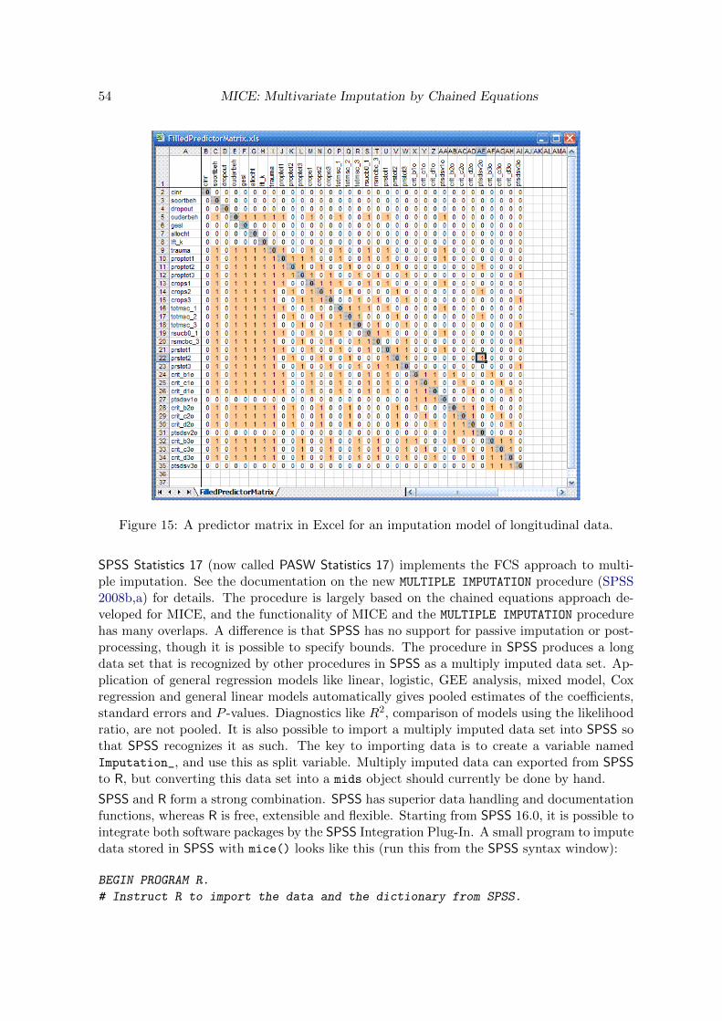
54 MICE: Multivariate Imputation by Chained Equations
Figure 15: A predictor matrix in Excel for an imputation model of longitudinal data.
SPSS Statistics 17 (now called PASW Statistics 17) implements the FCS approach to multi-ple imputation. See the documentation on the new MULTIPLE IMPUTATION procedure (SPSS2008b,a) for details. The procedure is largely based on the chained equations approach de-veloped for MICE, and the functionality of MICE and the MULTIPLE IMPUTATION procedurehas many overlaps. A difference is that SPSS has no support for passive imputation or post-processing, though it is possible to specify bounds. The procedure in SPSS produces a longdata set that is recognized by other procedures in SPSS as a multiply imputed data set. Ap-plication of general regression models like linear, logistic, GEE analysis, mixed model, Coxregression and general linear models automatically gives pooled estimates of the coefficients,standard errors and P -values. Diagnostics like R2, comparison of models using the likelihoodratio, are not pooled. It is also possible to import a multiply imputed data set into SPSS sothat SPSS recognizes it as such. The key to importing data is to create a variable namedImputation_, and use this as split variable. Multiply imputed data can exported from SPSSto R, but converting this data set into a mids object should currently be done by hand.
SPSS and R form a strong combination. SPSS has superior data handling and documentationfunctions, whereas R is free, extensible and flexible. Starting from SPSS 16.0, it is possible tointegrate both software packages by the SPSS Integration Plug-In. A small program to imputedata stored in SPSS with mice() looks like this (run this from the SPSS syntax window):
BEGIN PROGRAM R.
# Instruct R to import the data and the dictionary from SPSS.
Journal of Statistical Software 55
dict <- spssdictionary.GetDictionaryFromSPSS()
data <- spssdata.GetDataFromSPSS()
# Load mice, impute and get the original + imputed data.
library(mice)
imp <- mice(data,maxit=10)
com <- complete(imp,"long",inc=TRUE)
com <- cbind(com, Imputation_ = as.integer(com$.imp)-1)
# Export imputed data and dictionary from R to SPSS.
spssdictionary.SetDictionaryToSPSS("com", dict)
spssdata.SetDataToSPSS("com", com)
spssdictionary.EndDataStep()
END PROGRAM.
7.3. MItools
MItools (version 2.0) is a small R package available from CRAN written by T. Lumley containingtools for analyzing and pooling multiply imputed data. The multiply imputed data shouldbe of class ImputationList. A mids object (imp) can be transformed into an object of classImputationList object as follows:
> library(mitools)
> mydata <- imputationList(lapply(1:5, complete, x=imp))
Statistical analyses on these data can be done by with():
> fit <- with(mydata, expr=lm(..˜.. + ..)))
The pooled outcomes are obtained with summary(MIcombine(fit)). MIcombine() can beused for all fit objects for which a vcov() function exists, like our function pool(). Sincethis function does not exists for objects of class lme, pooling of mixed models is not possiblewith MItools. The package itself has no functions for creating imputations.
7.4. Zelig
The package Zelig (version 3.4-6, Imai et al. (2008)) offers a framework with a simple structureand syntax that encompasses a number of existing statistical methods. One of the functionsof Zelig is mi() which makes a list of imputed data sets of class mi. Zelig does not containfunctions for generating multiple imputations. When a data set of class mi is passed to thegeneral modeling function zelig(), it is recognized as an imputed data set. For a numberof modeling functions in Zelig the outcomes are then automatically pooled when the data issuch a list of imputed data sets. It is however not clear for which modeling function thisworks (ls.mixed() does not seem to be supported). The code for estimating the propensityscore model for hc (c.f. section 4.5) with zelig() is as follows:
> library(Zelig)
> imp <- cbind.mids(imp,data.frame(Rhc=is.na(boys$hc)))

56 MICE: Multivariate Imputation by Chained Equations
> mydata2 <- mi(complete(imp,1), complete(imp,2), complete(imp,3),
+ complete(imp,4),complete(imp,5))
> fit <- zelig(Rhc˜age+wgt+hgt+bmi+gen+phb+tv+reg, model="logit",
+ data=mydata2)
> summary(fit)
Model: logit
Number of multiply imputed data sets: 5
Combined results:
Call:
zelig(formula = r.hc ˜ age + wgt + hgt + bmi + gen + phb + tv +
reg, model = "logit", data = mydata2)
Coefficients:
Value Std. Error t-stat p-value
(Intercept) -3.091270 1.269657 -2.43473 0.0175574
age 0.120934 0.038184 3.16712 0.0018156
wgt -0.003175 0.018174 -0.17468 0.8620770
....
The result of zelig() is not as detailed as pool(), since the confidence intervals of theestimates and the fraction of missing information are not printed.
7.5. mi
mi is a new R package (version 0.0.7-2) for multiple imputation ((Su et al. 2009)). Theimputation method used in mi is also based on the FCS principle, and as in Zelig is called mi().The package contains modeling functions that pull together the estimates (point estimatesand their standard errors) from multiply imputed data sets for several models like lm(), glm()and lmer(). The package is quite extensive, and complements our package in some aspects,e.g. other facilities for diagnostic checking. The internal structure of class mi and class mids
is different, but it would certainly be useful to have conversion functions mi2mids() andmids2mi() in order to be able to combine the strengths of both packages.
8. Conclusion
The principle of fully conditional specification (FCS) has now gained wide acceptance. Goodsoftware is now available. Many applications using FCS have appeared, and many more willfollow. This paper documents a major update of MICE. FCS has recently been adopted andimplemented by SPSS, and was advertised by SPSS as the major methodological improvementof SPSS Statistics 17.
In the years to come, attention will shift from computational issues to the question how wecan apply the methodology in a responsible way. We need guidelines on how to report MI, weneed a better understanding of the dangers and limitations of the technique, we need pooling
Journal of Statistical Software 57
methods for special distributions, and we need entry-level texts that explain the idea and thatdemonstrate how to use the techniques in practice. Assuming that this all happens, multipleimputation using FCS will prove to be a great addition to our statistical tool chest.
Acknowledgement: Many people have been helpful in converting the original S-PLUS libraryinto the R package mice. We thank Jason Turner, Peter Malewski, Frank E. Harrell, JohnFox and Roel de Jong for their valuable contributions.
References
Abayomi K, Gelman A, Levy M (2008). “Diagnostics for multivariate imputations.” Journalof the Royal Statistical Society Series C: Applied Statistics, 57(3), 273–291.
Adamczyk A, Palmer I (2008). “Religion and initiation into marijuana use: The deterringrole of religious friends.” Journal of Drug Issues, 38(3), 717–741.
Alati R, Al Mamun A, Williams GM, O’Callaghan M, Najman JM, Bor W (2006). “In uteroalcohol exposure and prediction of alcohol disorders in early adulthood: A birth cohortstudy.” Archives of General Psychiatry, 63(9), 1009–1016.
Albert PS, Follmann D (2009). “Shared-parameter models.” In G Fitzmaurice, M Davidian,G Verbeke, G Molenberghs (eds.), “Longitudinal data analysis,” chapter 18, pp. 433–452.CRC Press, Boca Raton, FL.
Ambler G, Omar RZ, Royston P, Kinsman R, Keogh BE, Taylor KM (2005). “Generic, simplerisk stratification model for heart valve surgery.” Circulation, 112(2), 224–231.
Arnold BC, Castillo E, Sarabia JM (1999). Conditional specification of statistical models.Springer, New York.
Arnold BC, Press SJ (1989). “Compatible Conditional Distributions.” Journal of the AmericanStatistical Association, 84, 152–156.
Barnard J, Rubin DB (1999). “Small sample degrees of freedom with multiple imputation.”Biometrika, 86, 948–955.
Barosi G, Bergamaschi G, Marchetti M, Vannucchi AM, Guglielmelli P, Antonioli E, MassaM, Rosti V, Campanelli R, Villani L, Viarengo G, Gattoni E, Gerli G, Specchia G, TinelliC, Rambaldi A, Barbui T (2007). “JAK2 V617F mutational status predicts progression tolarge splenomegaly and leukemic transformation in primary myelofibrosis.” Blood, 110(12),4030–4036.
Brand JPL (1999). Development, implementation and evaluation of multiple imputationstrategies for the statistical analysis of incomplete data sets. Erasmus University, Rot-terdam.
Briggs A, Clark T, Wolstenholme J, Clarke P (2003). “Missing....presumed at random: Cost-analysis of incomplete data.” Health Economics, 12(5), 377–392.

58 MICE: Multivariate Imputation by Chained Equations
Brunner EJ, Chandola T, Marmot MG (2007). “Prospective effect of job strain on generaland central obesity in the Whitehall II Study.” American Journal of Epidemiology, 165(7),828–837.
Burton A, Billingham LJ, Bryan S (2007). “Cost-effectiveness in clinical trials: Using multipleimputation to deal with incomplete cost data.” Clinical Trials, 4(2), 154–161.
Butler RJ, Heron J (2008). “The prevalence of infrequent bedwetting and nocturnal enuresisin childhood.” Scandinavian Journal of Urology and Nephrology, 42(3), 257–264.
Byrne J, Spence MS, Fretz E, Mildenberger R, Chase A, Berry B, Pi D, Janssen C, Klinke P,Hilton D (2009). “Body Mass Index, Periprocedural Bleeding, and Outcome Following Per-cutaneous Coronary Intervention (from the British Columbia Cardiac Registry).” AmericanJournal of Cardiology, 103(4), 507–511.
Caria MP, Bellocco R, Zambon A, Horton NJ, Galanti MR (2009). “Overweight and perceptionof overweight as predictors of smokeless tobacco use and of cigarette smoking in a cohortof Swedish adolescents.” Addiction, 104(4), 661–668.
Chamberlain LJ, Crowley M, Tope D, Hodson R (2008). “Sexual harassment in organizationalcontext.” Work and Occupations, 35(3), 262–295.
Chase AJ, Fretz EB, Warburton WP, Klinke WP, Carere RG, Pi D, Berry B, Hilton JD (2008).“Association of the arterial access site at angioplasty with transfusion and mortality: TheM.O.R.T.A.L study (Mortality benefit of Reduced Transfusion after percutaneous coronaryintervention via the Arm or Leg).” Heart, 94(8), 1019–1025.
Clark TG, Altman DG (2003). “Developing a prognostic model in the presence of missingdata: An ovarian cancer case study.” Journal of Clinical Epidemiology, 56(1), 28–37.
Clark TG, Bradburn MJ, Love SB, Altman DG (2003). “Survival analysis part IV: Furtherconcepts and methods in survival analysis.” British Journal of Cancer, 89(5), 781–786.
Clark TG, Stewart ME, Altman DG, Gabra H, Smyth JF (2001). “A prognostic model forovarian cancer.” British Journal of Cancer, 85(7), 944–952.
Collins LM, Schafer JL, Kam CM (2001). “A comparison of inclusive and restrictive strategiesin modern missing data procedures.” Psychological Methods, 6(3), 330–351.
Cook RD, Weisberg S (1999). Applied regression including computing and graphics. Wiley,New York.
Cottrell G, Mary JY, Barro D, Cot M (2005). “Is malarial placental infection related toperipheral infection at any time of pregnancy?” American Journal of Tropical Medicineand Hygiene, 73(6), 1112–1118.
Cottrell G, Mary JY, Barro D, Cot M (2007). “The importance of the period of malarialinfection during pregnancy on birth weight in tropical Africa.” American Journal of TropicalMedicine and Hygiene, 76(5), 849–854.
Cummings P, Rivara FP, Olson CM, Smith KM (2006). “Changes in traffic crash mortalityrates attributed to use of alcohol, or lack of a seat belt, air bag, motorcycle helmet, orbicycle helmet, United States, 1982-2001.” Injury Prevention, 12(3), 148–154.

Journal of Statistical Software 59
Deave T, Heron J, Evans J, Emond A (2008). “The impact of maternal depression in preg-nancy on early child development.” BJOG: An International Journal of Obstetrics andGynaecology, 115(8), 1043–1051.
Den Hartog JE, Lardenoije CMJG, Severens JL, Land JA, Evers JLH, Kessels AGH (2008).“Screening strategies for tubal factor subfertility.” Human Reproduction, 23(8), 1840–1848.
Drechsler J, Rassler S (2008). “Does Convergence Really Matter?” In Shalabh, C Heumann(eds.), “Recent Advances in Linear Models and Related Areas. Essays in Honour of HelgeToutenburg,” pp. 341–355. Springer, Berlin.
Fernandes AS, Jarman IH, Etchells TA, Fonseca JM, Biganzoli E, Bajdik C, Lisboa PJG(2008). “Missing data imputation in longitudinal cohort studies - Application of PLANN-ARD in breast cancer survival.” In “Proceedings - 7th International Conference on MachineLearning and Applications, ICMLA 2008,” pp. 644–649.
Finke R, Adamczyk A (2008). “Cross-national moral beliefs: The influence of national religiouscontext.” Sociological Quarterly, 49(4), 617–652.
Garabed RB, Johnson WO, Gill J, Perez AM, Thurmond MC (2008). “Exploration of as-sociations between governance and economics and country level foot-and-mouth diseasestatus by using Bayesian model averaging.” Journal of the Royal Statistical Society.SeriesA: Statistics in Society, 171(3), 699–722.
Gelman A (2004). “Parameterization and Bayesian modeling.” Journal of the AmericanStatistical Association, 99(466), 537–545.
Gelman A, Raghunathan TE (2001). “Discussion of Arnold et al. “Conditionally specifieddistributions”.” Statistical Science, 16, 249–274.
Gerestein CG, Eijkemans MJC, De Jong D, Van Der Burg MEL, Dykgraaf RHM, Kooi GS,Baalbergen A, Burger CW, Ansink AC (2009). “The prediction of progression-free andoverall survival in women with an advanced stage of epithelial ovarian carcinoma.” BJOG:An International Journal of Obstetrics and Gynaecology, 116(3), 372–380.
Giorgi R, Belot A, Gaudart J, Launoy G, the French Network of Cancer Registries FRANCIM(2008). “The performance of multiple imputation for missing covariate data within thecontext of regression relative survival analysis.” Statistics in Medicine, 27(30), 6310–6331.
Goldstein H, Carpenter J, Kenward MG, Levin KA (2009). “Multilevel models with multi-variate mixed response types.” Statistical Modelling. In press.
Grote FK, Oostdijk W, Muinck Keizer-Schrama SM, Dekker FW, van Dommelen P, vanBuuren S, Lodder-van der Kooij AM, Verkerk PH, Wit JM (2007). “Referral patterns ofchildren with poor growth in primary health care.” BMC Public Health, 7, 77.
Grote FK, van Dommelen P, Oostdijk W, de Muinck Keizer-Schrama SMPF, Verkerk PH,Wit JM, van Buuren S (2008). “Developing evidence-based guidelines for referral for shortstature.” Archives of Disease in Childhood, 93(3), 212–217.
Harel O (2009). “The estimation of R2 and adjusted R2 in incomplete data sets using multipleimputation.” Journal of Applied Statistics, in press.

60 MICE: Multivariate Imputation by Chained Equations
Harrell FE (2001). Regression modeling strategies, with applications to linear models, logisticregression, and survival analysis. Springer, New York.
Heckerman D, Chickering DM, Meek C, Rounthwaite R, Kadie C (2001). “Dependency Net-works for Inference, Collaborative Filtering, and Data Visualisation.” Journal of MachineLearning Research, 1, 49–75.
Herman-Giddens M, Slora E, Wasserman R, Bourdony C, Bhapkar M, Koch C, Hasemeier C(1997). “Secondary sexual characteristics and menses in young girls seen in office practice:A study from the pediatric research in office settings network.” Pediatrics, 99(4), 505–512.
Heymans MW, van Buuren S, Knol DL, Van Mechelen W, De Vet HCW (2007). “Variableselection under multiple imputation using the bootstrap in a prognostic study.” BMC Med-ical Research Methodology, 7, 33. URL http://www.stefvanbuuren.nl/publications/
Variable%20selection%20-%20BMC%20MRM%202007.pdf.
Hill JL, Reiter JP, Zanutto EL (2004). “A comparison of experimental and observational dataanalyses.” In A Gelman, XL Meng (eds.), “Applied Bayesian modeling and causal inferencefrom incomplete-data perspectives,” chapter 5, pp. 49–60. Wiley, New York.
Hille ETM, Elbertse L, nebroek Gravenhorst J, Brand R, Verloove-Vanhorick SP (2005).“Nonresponse bias in a follow-up study of 19-year-old adolescents born as preterm infants.”Pediatrics, 116(5).
Hille ETM, Weisglas-Kuperus N, Van Goudoever JB, Jacobusse GW, Ens-Dokkum MH,De Groot L, Wit JM, Geven WB, Kok JH, De Kleine MJK, Kollee LAA, Mulder ALM,Van Straaten HLM, De Vries LS, Van Weissenbruch MM, Verloove-Vanhorick SP (2007).“Functional outcomes and participation in young adulthood for very preterm and very lowbirth weight infants: The Dutch project on preterm and small for gestational age infantsat 19 years of age.” Pediatrics, 120(3).
Hindorff LA, Rice KM, Lange LA, Diehr P, Halder I, Walston J, Kwok P, Ziv E, Nievergelt C,Cummings SR, Newman AB, Tracy RP, Psaty BM, Reiner AP (2008). “Common variantsin the CRP gene in relation to longevity and cause-specific mortality in older adults: TheCardiovascular Health Study.” Atherosclerosis, 197(2), 922–930.
Horton NJ, Kleinman KP (2007). “Much ado about nothing: A comparison of missing datamethods and software to fit incomplete data regression models.” American Statistician,61(1), 79–90.
Horton NJ, Lipsitz SR (2001). “Multiple imputation in practice: Comparison of softwarepackages for regression models with missing variables.” American Statistician, 55, 244–254.
Horwood J, Salvi G, Thomas K, Duffy L, Gunnell D, Hollis C, Lewis G, Menezes P, ThompsonA, Wolke D, Zammit S, Harrison G (2008). “IQ and non-clinical psychotic symptoms in 12-year-olds: Results from the ALSPAC birth cohort.” British Journal of Psychiatry, 193(3),185–191.
Hox JJ (2002). Multilevel analysis. Techniques and applications. Lawrence Erlbaum Asso-ciates, Inc., Mahwah, NJ.

Journal of Statistical Software 61
Huo D, Adebamowo CA, Ogundiran TO, Akang EE, Campbell O, Adenipekun A, CummingsS, Fackenthal J, Ademuyiwa F, Ahsan H, Olopade OI (2008). “Parity and breastfeedingare protective against breast cancer in Nigerian women.” British Journal of Cancer, 98(5),992–996.
Imai K, King G, Lau O (2008). “Toward a common framework for statistical analysis anddevelopment.” Journal of Computational and Graphical Statistics, 17(4), 1–22.
Ip EH, Wang YJ (2009). “Canonical representation of conditionally specified multivariatediscrete distributions.” Journal of Multivariate Analysis, 100(6), 1282–1290.
Jacobusse GW (2005). WinMICE user’s manual. TNO Quality of Life, Leiden. URL http:
//www.multiple-imputation.com/.
Jensen M, Roy A (2008). “Staging exchange partner choices: When do status and reputationmatter?” Academy of Management Journal, 51(3), 495–516.
Kasim RM, Raudenbush SW (1998). “Application of Gibbs sampling to nested variancecomponents models with heterogeneous within-group variance.” Journal of Educationaland Behavioral Statistics, 23(2), 93–116.
Kekitiinwa A, Lee KJ, Walker AS, Maganda A, Doerholt K, Kitaka SB, Asiimwe A, Judd A,Musoke P, Gibb DM (2008). “Differences in factors associated with initial growth, CD4, andviral load responses to ART in HIV-infected children in Kampala, Uganda, and the UnitedKingdom/Ireland.” Journal of Acquired Immune Deficiency Syndromes, 49(4), 384–392.
Kennickell AB (1991). “Imputation of the 1989 survey of consumer finances: Stochasticrelaxation and multiple imputation.” ASA 1991 Proceedings of the Section on Survey Re-searchMethods, pp. 1–10.
Klein LW, Kolm P, Xu X, Krone RJ, Anderson HV, Rumsfeld JS, Brindis RG, WeintraubWS (2009). “A Longitudinal Assessment of Coronary Interventional Program Quality. AReport From the American College of Cardiology-National Cardiovascular Data Registry.”JACC: Cardiovascular Interventions, 2(2), 136–143.
Klein MB, MacK CD, Kramer CB, Heimbach DM, Gibran NS, Rivara FP (2008). “Influenceof injury characteristics and payer status on burn treatment location in Washington State.”Journal of Burn Care and Research, 29(3), 435–440.
Kleinbaum DG, Kupper LL, Muller KE (1988). Applied regression analysis and other multi-variate methods (second edition). PWS-Kent, Boston.
Li KH, Meng XL, Raghunathan TE, Rubin DB (1991). “Significance levels from repeatedp-values with multiply-imputed data.” Statistica Sinica, 1, 65–92.
Little RJA (1988). “Missing data adjustments in large surveys (with discussion).” Journal ofBusiness Economics and Statistics, 6, 287–301.
Little RJA (2009a). “Comments on: Missing data methods in longitudinal studies: a review.”Test, 18, 47–50.

62 MICE: Multivariate Imputation by Chained Equations
Little RJA (2009b). “Selection and pattern-mixture models.” In G Fitzmaurice, M Davidian,G Verbeke, G Molenberghs (eds.), “Longitudinal data analysis,” chapter 18, pp. 409–431.CRC Press, Boca Raton, FL.
Little RJA, Rubin DB (2002). Statistical analysis with missing data (second edition). Wiley,New York.
Macleod J, Hickman M, Bowen E, Alati R, Tilling K, Smith GD (2008). “Parental drug use,early adversities, later childhood problems and children’s use of tobacco and alcohol at age10: Birth cohort study.” Addiction, 103(10), 1731–1743.
Marshall A, Billingham LJ, Bryan S (2009). “Can we afford to ignore missing data in cost-effectiveness analyses?” European Journal of Health Economics, 10(1), 1–3.
McCaul KA, Fritschi L, Baade P, Coory M (2008). “The incidence of second primary invasivemelanoma in Queensland, 1982-2003.” Cancer Causes and Control, 19(5), 451–458.
McClelland RL, Kronmal RA, Haessler J, Blumenthal RS, Goff J (2008). “Estimation ofrisk factor associations when the response is influenced by medication use: An imputationapproach.” Statistics in Medicine, 27(24), 5039–5053.
Melhem NM, Brent DA, Ziegler M, Iyengar S, Kolko D, Oquendo M, Birmaher B, Burke A,Zelazny J, Stanley B, Mann JJ (2007). “Familial pathways to early-onset suicidal behavior:Familial and individual antecedents of suicidal behavior.” American Journal of Psychiatry,164(9), 1364–1370.
Meng XL (1995). “Multiple imputation with uncongenial sources of input (with discusson).”Statistical Science, (10), 538–573.
Meng XL, Rubin DB (1992). “Performing likelihood ratio tests with multiple-imputed datasets.” Biometrika, 79(1), 103–111.
Michel L, Giorgi R, Villes V, Poizot-Martin I, Dellamonica P, Spire B, Protopopescu C,Carrieri MP (2009). “Withdrawal symptoms as a predictor of mortality in patients HIV-infected through drug use and receiving highly active antiretroviral therapy (HAART).”Drug and Alcohol Dependence, 99(1-3), 96–104.
Moons KGM, Donders R, Stijnen T, Harrell F (2006). “Using the outcome for imputation ofmissing predictor values was preferred.” Journal of Clinical Epidemiology, 59(10), 1092–1101.
Morgenstern M, Wiborg G, Isensee B, Hanewinkel R (2009). “School-based alcohol education:Results of a cluster-randomized controlled trial.” Addiction, 104(3), 402–412.
Mueller BA, Cummings P, Rivara FP, Brooks MA, Terasaki RD (2008). “Injuries of the head,face, and neck in relation to ski helmet use.” Epidemiology, 19(2), 270–276.
Mumtaz G, Tamim H, Kanaan M, Khawaja M, Khogali M, Wakim G, Yunis KA (2007). “Ef-fect of consanguinity on birth weight for gestational age in a developing country.” AmericanJournal of Epidemiology, 165(7), 742–752.

Journal of Statistical Software 63
Nash D, Katyal M, Brinkhof MWG, Keiser O, May M, Hughes R, Dabis F, Wood R, Sprinz E,Schechter M, Egger M (2008). “Long-term immunologic response to antiretroviral therapyin low-income countries: A collaborative analysis of prospective studies.” AIDS, 22(17),2291–2302.
O’Callaghan FV, O’Callaghan M, Najman JM, Williams GM, Bor W, Alati R (2006). “Pre-diction of adolescent smoking from family and social risk factors at 5 years, and maternalsmoking in pregnancy and at 5 and 14 years.” Addiction, 101(2), 282–290.
Orsini N, Bellocco R, Bottai M, Pagano M, Michaelsson K, Wolk A (2008a). “Combinedeffects of obesity and physical activity in predicting mortality among men.” Journal ofInternal Medicine, 264(5), 442–451.
Orsini N, Mantzoros CS, Wolk A (2008b). “Association of physical activity with cancerincidence, mortality, and survival: A population-based study of men.” British Journal ofCancer, 98(11), 1864–1869.
Oudshoorn K, van Buuren S, van Rijckevorsel J (1999). Flexible multiple imputationby chained equations of the AVO-95 Survey, volume PG/VGZ/00.045. TNO Preven-tion and Health, Leiden. URL http://www.stefvanbuuren.nl/publications/Flexible%
20multiple%20-%20TNO99045%201999.pdf.
Pedhazur EJ (1973). Multiple regression in behavioral research (second edition). Holt, Rine-hart and Winston, New York.
Prompers L, Schaper N, Apelqvist J, Edmonds M, Jude E, Mauricio D, Uccioli L, UrbancicV, Bakker K, Holstein P, Jirkovska A, Piaggesi A, Ragnarson-Tennvall G, Reike H, SpraulM, Van Acker K, Van Baal J, Van Merode F, Ferreira I, Huijberts M (2008). “Prediction ofoutcome in individuals with diabetic foot ulcers: Focus on the differences between individ-uals with and without peripheral arterial disease. The EURODIALE Study.” Diabetologia,51(5), 747–755.
Raghunathan T, Bondarenko I (2007). “Diagnostics for Multiple Imputations.” SSRN. URLhttp://ssrn.com/abstract=1031750.
Raghunathan TE, Lepkowski JM, van Hoewyk J, Solenberger P (2001). “A multivariatetechnique for multiply imputing missing values using a sequence of regression models.”Survey Methodology, 27, 85–95.
Rahman A, Reed E, Underwood M, Shipley ME, Omar RZ (2008). “Factors affecting self-efficacy and pain intensity in patients with chronic musculoskeletal pain seen in a specialistrheumatology pain clinic.” Rheumatology, 47(12), 1803–1808.
Ramchandani PG, Stein A, O’Connor TG, Heron J, Murray L, Evans J (2008). “Depression inmen in the postnatal period and later child psychopathology: A population cohort study.”Journal of the American Academy of Child and Adolescent Psychiatry, 47(4), 390–398.
Roudsari B, Field C, Caetano R (2008). “Clustered and missing data in the US NationalTrauma Data Bank: Implications for analysis.” Injury Prevention, 14(2), 96–100.

64 MICE: Multivariate Imputation by Chained Equations
Roudsari BS, Nathens AB, Cameron P, Civil I, Gruen RL, Koepsell TD, Lecky FE, LeferingRL, Liberman M, Mock CN, Oestern HJ, Schildhauer TA, Waydhas C, Rivara FP (2007).“International comparison of prehospital trauma care systems.” Injury, 38(9), 993–1000.
Rouxel A, Hejblum G, Bernier MO, Boelle PY, Menegaux F, Mansour G, Hoang C, AurengoA, Leenhardt L (2004). “Prognostic factors associated with the survival of patients devel-oping loco-regional recurrences of differentiated thyroid carcinomas.” Journal of ClinicalEndocrinology and Metabolism, 89(11), 5362–5368.
Royston P (2004). “Multiple imputation of missing values.” The Stata Journal, 4, 227–241.
Royston P (2005). “Multiple imputation of missing values: Update.” Stata Journal, 5(2),188–201.
Royston P, Parmar MKB, Sylvester R (2004). “Construction and validation of a prognosticmodel across several studies, with an application in superficial bladder cancer.” Statisticsin Medicine, 23(6), 907–926.
Rubin DB (1976). “Inference and missing data.” Biometrika, 63, 581–590.
Rubin DB (1987). Multiple imputation for nonresponse in surveys. Wiley, New York.
Rubin DB (1996). “Multiple Imputation after 18+ Years.” Journal of the American StatisticalAssociation, 91(434), 473–489.
Rubin DB (2003). “Nested multiple imputation of NMES via partially incompatible MCMC.”Statistica Neerlandica, 57(1), 3–18.
Rubin DM, Downes KJ, O’Reilly ALR, Mekonnen R, Luan X, Localio R (2008). “Impactof kinship care on behavioral well-being for children in out-of-home care.” Archives ofPediatrics and Adolescent Medicine, 162(6), 550–556.
Sabin CA, Lee KJ, Dunn D, Porter K, Bansi RGL, Hill T, Phillips AN, Schwenk A, LeenC, Delpech V, Anderson J, Gazzard B, Johnson M, Easterbrook P, Walsh J, Fisher M,Orkin C (2008). “Treatment switches after viral rebound in HIV-infected adults startingantiretroviral therapy: Multicentre cohort study: The United Kingdom Collaborative HIVCohort (CHIC) Study.” AIDS, 22(15), 1943–1950.
Samant IV UB, MacK CD, Koepsell T, Rivara FP, Vavilala MS (2008). “Time of hypoten-sion and discharge outcome in children with severe traumatic brain injury.” Journal ofNeurotrauma, 25(5), 495–502.
Schafer JL (1997). Analysis of incomplete multivariate data. Chapman & Hall, London.
Schafer JL, Yucel RM (2002). “Computational strategies for multivariate linear mixed-effectsmodels with missing values.” Journal of Computational and Graphical Statistics, 11(2),437–457.
Schnoll RA, Rukstalis M, Wileyto EP, Shields AE (2006). “Smoking Cessation Treatmentby Primary Care Physicians. An Update and Call for Training.” American Journal ofPreventive Medicine, 31(3), 233–239.

Journal of Statistical Software 65
Schunk D (2008). “A Markov chain Monte Carlo algorithm for multiple imputation in largesurveys.” Advances in Statistical Analysis, 92(1), 101–114.
Sharma R, Zucknick M, London R, Kacevska M, Liddle C, Clarke SJ (2008). “Systemic in-flammatory response predicts prognosis in patients with advanced-stage colorectal cancer.”Clinical Colorectal Cancer, 7(5), 331–337.
Shen Z (2000). Nested Multiple Imputation. Ph.D. thesis, Harvard University, Dept. ofStatistics.
Sisk JE, Hebert PL, Horowitz CR, McLaughlin MA, Wang JJ, Chassin MR (2006). “Effectsof nurse management on the quality of heart failure care in minority communities: Arandomized trial.” Annals of Internal Medicine, 145(4), 273–283.
Smith GCS, Crossley JA, Aitken DA, Pell JP, Cameron AD, Connor JM, Dobbie R (2004a).“First-trimester placentation and the risk of antepartum stillbirth.” Journal of the AmericanMedical Association, 292(18), 2249–2254.
Smith GCS, Wood AM, Pell JP, White IR, Crossley JA, Dobbie R (2004b). “Second-trimestermaternal serum levels of alpha-fetoprotein and the subsequent risk of sudden infant deathsyndrome.” New England Journal of Medicine, 351(10), 978–986.
Solutions S (2001). SOLAS for Missing Data Analysis. Statistical Solutions, Cork, Ireland.
Sommer M, Geurts JWJM, Stessel B, Kessels AGH, Peters ML, Patijn J, Van Kleef M, KremerB, Marcus MAE (2009). “Prevalence and predictors of postoperative pain after ear, nose,and throat surgery.” Archives of Otolaryngology - Head and Neck Surgery, 135(2), 124–130.
Souverein OW, Zwinderman AH, Tanck MWT (2006). “Multiple imputation of missing geno-type data for unrelated individuals.” Annals of Human Genetics, 70(3), 372–381.
SPSS (2008a). SPSS 17 Algorithms. SPSS Inc., Chicago, IL.
SPSS (2008b). SPSS 17 Missing Values. SPSS Inc., Chicago, IL.
Su YS, Gelman A, Hill J, M Y (2009). “Multiple Imputation with Diagnostics (mi) in R:Opening Windows into the Black Box.” Journal of Statistical Software, (forthcoming).
Sundell K, Hansson K, Lofholm CA, Olsson T, Gustle LH, Kadesjo C (2008). “The Trans-portability of Multisystemic Therapy to Sweden: Short-Term Results From a RandomizedTrial of Conduct-Disordered Youths.” Journal of Family Psychology, 22(4), 550–560.
Tanasoiu C, Colonescu C (2008). “Determinants of support for european integration: Thecase of bulgaria.” European Union Politics, 9(3), 363–377.
Templ M, Filzmoser P (2008). Visualization of missing values using the R-package VIM.Institut f. Statistik u. Wahrscheinlichkeitstheorie, Wien. URL http://www.statistik.
tuwien.ac.at/forschung/CS/CS-2008-1complete.pdf.
Thein HH, Yi Q, Dore GJ, Krahn MD (2008). “Natural history of hepatitis C virus infectionin HIV-infected individuals and the impact of HIV in the era of highly active antiretroviraltherapy: A meta-analysis.” AIDS, 22(15), 1979–1991.
66 MICE: Multivariate Imputation by Chained Equations
Tiemeier H, Van Dijck W, Hofman A, Witteman JCM, Stijnen T, Breteler MMB (2004).“Relationship between Atherosclerosis and Late-Life Depression: The Rotterdam Study.”Archives of General Psychiatry, 61(4), 369–376.
Ton TGN, Longstreth J, Koepsell T (2009). “Active and passive smoking and risk of narcolepsyin people with HLA DQB1*0602: A population-based case-control study.” Neuroepidemi-ology, 32(2), 114–121.
van Buuren S (2007). “Multiple imputation of discrete and continuous data by fully conditionalspecification.” Statistical Methods in Medical Research, 16(3), 219–242. URL http://www.
stefvanbuuren.nl/publications/MI%20by%20FCS%20-%20SMMR%202007.pdf.
van Buuren S (2010). “Multiple imputation of multilevel data.” In J Hox, K Roberts (eds.),“The Handbook of Advanced Multilevel Analysis,” chapter 0, pp. 000–000. Routledge, Mil-ton Park, UK.
van Buuren S, Boshuizen HC, Knook DL (1999). “Multiple imputation of miss-ing blood pressure covariates in survival analysis.” Statistics in Medicine, 18(6),681–694. URL http://www.stefvanbuuren.nl/publications/Multiple%20imputation%
20-%20Stat%20Med%201999.pdf.
van Buuren S, Boshuizen HC, Reijneveld SA (2006a). “Toward targeted hypertension screeningguidelines.” Medical Decision Making, 26(2), 145–153. URL http://www.stefvanbuuren.
nl/publications/Hypertension%20-%20MDM%202006.pdf.
van Buuren S, Brand JPL, Groothuis-Oudshoorn CGM, Rubin DB (2006b). “Fully conditionalspecification in multivariate imputation.” Journal of Statistical Computation and Simula-tion, 76(12), 1049–1064. URL http://www.stefvanbuuren.nl/publications/FCS%20in%
20multivariate%20imputation%20-%20JSCS%202006.pdf.
van Buuren S, Oudshoorn K (2000). Multivariate Imputation by Chained Equations:MICE V1.0 User’s manual, volume PG/VGZ/00.038. TNO Prevention and Health,Leiden. URL http://www.stefvanbuuren.nl/publications/MICE%20V1.0%20Manual%
20TNO00038%202000.pdf.
Van Den Hout WB, Goekoop-Ruiterman YPM, Allaart CF, Vries-Bouwstra JKD, HazesJMM, Kerstens PJSM, Van Zeben D, Hulsmans HMJ, De Jonge-Bok JM, De SonnavillePBJ, Dijkmans BAC, Breedveld FC (2009). “Cost-utility analysis of treatment strategiesin patients with recent-onset rheumatoid arthritis.” Arthritis Care and Research, 61(3),291–299.
van der Hulst M, Vollenbroek-Hutten M, Groothuis-Oudshoorn K, Hermens H (2008). “Mul-tidisciplinary Rehabilitation Treatment of Patients With Chronic Low Back Pain: A Prog-nostic Model for Its Outcome.” Clinical Journal of Pain, 24(5), 421–430.
Van Oijen M, De Jong FJ, Witteman JCM, Hofman A, Koudstaal PJ, Breteler MMB (2007).“Atherosclerosis and risk for dementia.” Annals of Neurology, 61(5), 403–410.
Van Vlierberghe L, Braet C, Goossens L, Rosseel Y, Mels S (2009). “Psychological disorder,symptom severity and weight loss in inpatient adolescent obesity treatment.” InternationalJournal of Pediatric Obesity, 4(1), 36–44.

Journal of Statistical Software 67
Van Wouwe JP, Lanting CI, van Dommelen P, Treffers PE, van Buuren S (2009). “Breast-feeding duration related to practised contraception in the Netherlands.” Acta Paediatrica,International Journal of Paediatrics, 98(1), 86–90. URL http://www.stefvanbuuren.nl/
publications/Breastfeeding%20duration%20-%20Acta%20Ped%202008.pdf.
Veenstra R, Lindenberg S, De Winter AF, Oldehinkel AJ, Verhulst FC, Ormel J (2005).“Bullying and victimization in elementary schools: A comparison of bullies, victims,bully/victims, and uninvolved preadolescents.” Developmental Psychology, 41(4), 672–682.
Venables WN, Ripley BD (2002). Modern applied statistics with S (fourth edition). Springer-Verlag, New York.
Walker AS, Mulenga V, Sinyinza F, Lishimpi K, Nunn A, Chintu C, Gibb DM (2006). “Deter-minants of survival without antiretroviral therapy after infancy in HIV-1-infected Zambianchildren in the CHAP trial.” Journal of Acquired Immune Deficiency Syndromes, 42(5),637–645.
Ward L, Franks P (2007). “Changes in health care expenditure associated with gaining orlosing health insurance.” Annals of Internal Medicine, 146(11), 768–774.
White I, Daniel R, Royston P (2009). “Avoiding bias due to perfect prediction in multipleimputation of incomplete categorical variables.” submitted for publication.
Wiles NJ, Jones GT, Haase AM, Lawlor DA, Macfarlane GJ, Lewis G (2008). “Physicalactivity and emotional problems amongst adolescents.” Social Psychiatry and PsychiatricEpidemiology, 43(10), 765–772.
Wolfe F, Caplan L, Michaud K (2006). “Treatment for rheumatoid arthritis and the risk of hos-pitalization for pneumonia: Associations with prednisone, disease-modifying antirheumaticdrugs, and anti-tumor necrosis factor therapy.” Arthritis and Rheumatism, 54(2), 628–634.
Wood AM, White IR, Royston P (2008). “How should variable selection be performed withmultiply imputed data?” Statistics in Medicine, 27(17), 3227–3246.
Yu LM, Burton A, Rivero-Arias O (2007). “Evaluation of software for multiple imputation ofsemi-continuous data.” Statistical Methods in Medical Research, 16, 243–258.
Yucel RM (2008). “Multiple imputation inference for multivariate multilevel continuous datawith ignorable non-response.” Philosophical Transactions of the Royal Society A, 366,2389–2403.

68 MICE: Multivariate Imputation by Chained Equations
Affiliation:
Stef van Buuren
1) Department of StatisticsTNO Quality of LifeP.O. Box 22152301 CE Leiden, The Netherlands2) Department of Methodology and Statistics, FSSUniversity of UtrechtE-mail: [email protected]: http://www.stefvanbuuren.nl
Karin Groothuis-Oudshoorn
1) Roessingh Research and DevelopmentP.O. Box 3107500 AH Enschede, The Netherlands2) University of Twente, EnschedeE-mail: [email protected]
Journal of Statistical Software http://www.jstatsoft.org/
published by the American Statistical Association http://www.amstat.org/
Volume VV, Issue II Submitted: yyyy-mm-ddMMMMMM YYYY Accepted: yyyy-mm-dd