mesoscale mapping capabilities of multisatellite altimeter missions: first results with real data in...

s 65 (2007) 190–211www.elsevier.com/locate/jmarsys

Journal of Marine System

Mesoscale mapping capabilities of multisatellite altimeter missions:First results with real data in the Mediterranean Sea

Ananda Pascual a,⁎, Marie-Isabelle Pujol a, Gilles Larnicol a,Pierre-Yves Le Traon a, Marie-Hélène Rio b

a CLS, Space Oceanography Division, Toulouse, Franceb Istituto di Scienze dell'Atmosfera e del Clima, Rome, Italy

Received 23 September 2004; accepted 23 December 2004Available online 30 October 2006

Abstract

Four altimeter missions [Jason-1, ERS-2, TOPEX/POSEIDON interleaved with Jason-1 (T/P) and Geosat Follow-On (GFO)]are intercalibrated and merged in an objective analysis scheme with the aim of improving the estimation of mesoscale surface oceancirculation in the Mediterranean Sea. A validation with independent altimetric data shows that, with the combination of threealtimeters, in regions of large mesoscale variability, the sea level and velocity can be mapped with a relative accuracy of about 6%and 23%, respectively, which is a factor of 2.2 less than the results derived from Jason-1 alone, and a factor of about 1.5 less thanthe results obtained from Jason-1+ERS-2. Mean eddy kinetic energy (EKE) is computed from the different altimeterconfigurations. It shows that the combination of Jason-1+ERS-2 fails to reproduce some intense signals. On the contrary, when T/Pis added, these features are well recovered and the EKE does not show significant discontinuities due to sampling effects. Theimpact of the fourth mission (GFO) is less critical but it also improves the representation of energetic structures. In average, themerged Jason-1+ERS-2+T/P+GFO maps yield EKE levels 15% higher than Jason-1+ERS-2. Finally, we show that theconsistency between altimetry and Sea Surface Temperature, drifting buoys and tide gauges, is significantly improved when foursatellites are merged compared to the results derived from the two-satellite configuration. This study demonstrates that, at leastthree, but preferably four, altimeter missions are needed for monitoring the Mediterranean mesoscale circulation.© 2006 Elsevier B.V. All rights reserved.

Keywords: Satellite altimetry; Sea level; Eddy Kinetic Energy; Mesoscale ocean circulation; Mediterranean Sea

1. Introduction

Satellite altimetry is considered as one of the mostimportant input datasets for operational applications, as itprovides surface dynamic topography measurements,which constitute a strong constraint to estimate and fore-

⁎ Corresponding author. Present address: Institut Mediterrani d'Es-tudis Avançats, IMEDEA, (CSIC-UIB), C/Miquel Marquès, 21; 07190Esporles; Mallorca, Spain. Tel.: +34 971 611732; fax: +34 971 611761.

E-mail address: [email protected] (A. Pascual).

0924-7963/$ - see front matter © 2006 Elsevier B.V. All rights reserved.doi:10.1016/j.jmarsys.2004.12.004

cast the three-dimensional ocean state through dataassimilation. One requirement for satellite altimetry isthat at least two altimeter missions are needed to resolvethe main space and time scales of the ocean (Koblinsky etal., 1992). The contribution of merging two altimetricmissions, TOPEX/Poseidon (T/P) and ERS-1/2, has beenwell illustrated by Ducet et al. (2000) and Ducet and LeTraon (2001). In the Mediterranean, the combination ofT/P+ERS-1/2 has also allowed a characterization of themajor changes in the Mediterranean Sea level variabilityfor the 1993–1999 period (Larnicol et al., 2002).

mailto:[email protected]

http://dx.doi.org/10.1016/j.jmarsys.2004.12.004

191A. Pascual et al. / Journal of Marine Systems 65 (2007) 190–211

Several theoretical studies have explored the impactof merging multiple-satellite altimeter missions usingsimulated data. Greenslade et al. (1997) concluded thatonly the large-scale signal can be fully resolved witheven three or four satellites. On the contrary, Le Traonand Dibarboure (1999) found that a combination ofthree satellites can actually provide an importantreduction of the velocity mean mapping error withrespect to one or two satellites (errors below 10% of thesignal variance). Le Traon et al. (2001) and Le Traonand Dibarboure (2002) carried out a similar analysis butusing a high-resolution numerical model that reproducesquite well the mesoscale in the North Atlantic. Theirmain conclusion was that high-frequency signals, notcorrectly sampled by any combination of satellites (up to4), accounted for an important contribution of thevelocity mapping errors (15% to 20%).

Le Traon et al. (2003) have successfully carried out afirst merging of GEOSAT Follow-On with T/P andERS-2. They underlined the importance of reducingmeasurement errors and inconsistencies between differ-ent missions as well as the importance of a preciseestimate of a GEOSAT Follow-On mean profile toobtain coherent data sets.

As a follow-on to the T/P mission, the French/USaltimetric satellite Jason-1 was launched in December2001. Since mid-September 2002, T/P has been flyingmidway between two adjacent Jason-1 ground-tracks.This has resulted in a track separation half that of the T/Pmission, offering a much improved sampling for thestudy of mesoscale variability. In fact, Fu et al. (2003)and Le Traon and Dibarboure (2004) have alreadyevidenced the improved spatial resolution of sea surfaceheight from the Tandem T/P–Jason-1 mission comparedto T/P or Jason-1 alone. Fu et al. (2003) have founddifferences as large as 40 cm in the western NorthAtlantic between the tandem mission and Jason-1 alone.Le Traon and Dibarboure (2004) have shown that, inareas of intense variability the sea level and velocity canbe mapped, respectively, with an accuracy of about 6%and 20% to 30%, which is a factor of two less than theresults derived from T/P or Jason-1 alone. Their resultsare consistent with Le Traon et al. (2001) and Le Traonand Dibarboure (2002) theoretical analyses. However,in none of these works any attempt to combine real datafrom four altimeter missions has been performed.

In this work we present the first results of mergingreal data from these four altimeters, with the aim ofobtaining high-resolution maps capable of monitoringthe mesoscale variability. The selected region is theMediterranean Sea. The Mediterranean is known (e.g.Larnicol et al., 2002; Hamad et al., 2005) to be an area of

complex spatio/temporal variability, where the meso-scale structures have a typical size of about 100 km,which is not fully resolved by only two altimeters (LeTraon and Dibarboure, 2004; Tai, 1998). Furthermore,the signals in the Mediterranean are quite weak, of about7–8 cm rms (Larnicol et al., 2002), and almost half ofthe variability is due to large-scale steric signals. Theremaining signals, basically associated with the meso-scale variability, are at the limit of the present altimeters'accuracy. As a consequence, the adjustment/intercali-bration between the different altimeters and thecomputation of an accurate mean sea level (to beremoved from the sea surface height in order to obtainsea level anomalies) are a crucial issue. The Mediter-ranean, in summary, appears a challenging region for amulti-satellite combination.

The paper is organized as follows: in Section 2 thedataset and data processing are presented. We also detailthe objective analysis methodology and the sampling forthe different altimeter configurations. Section 3 isentirely devoted to presenting the results. First (inSection 3.1), we show the mapping error associated witheach combination of satellites. Next (in Section 3.2), wecarry out a validation of the merged maps withindependent along track altimetric data in order toquantify the impact of the merging. The mean eddykinetic energy (EKE) obtained from the differentconfigurations is described and analyzed in Section3.3. In Section 3.4, altimetric data are compared to otherkind of data (SST, drifters and tide gauge data). Finally,in Section 4, the conclusions are outlined.

2. Datasets and data processing

2.1. Data processing

Eight months and a half of Jason-1, ERS-2, TOPEX/Poseidon interleaved (T/P) and Geosat Follow-On(GFO) delayed time data are used for this study.Jason-1 and T/P data are the M-GDR distributed byAVISO. ERS-2 data are distributed by ESA and GFOproducts by the National Oceanic and AtmosphericAdministration (NOAA). All the data sets span from thebeginning of the T/P inverleaved mission (October2002) to the end of the ERS-2 mission (mid June 2003).

For all datasets, the usual geophysical correctionshave been applied (wet and dry tropospheric, iono-spheric, electromagnetic, tides, inverse barometer, fordetails see Le Traon and Ogor, 1998; Le Traon et al.,2003 for specific corrections of GFO). Merging multi-satellite altimeter missions requires homogeneous andintercalibrated SSH data sets, especially in order to

192 A. Pascual et al. / Journal of Marine Systems 65 (2007) 190–211

reduce orbit errors of the less accurate ERS-2 and GFOmissions. Intercalibrated data sets are obtained byperforming a global crossover adjustment of the ERS-2, GFO and Jason-1 orbit, using the more precise T/Pdata as a reference (Le Traon and Ogor, 1998). Note thatJason-1 and T/P having the same accuracy, Jason-1could have also been selected as the reference mission.The data are then resampled every 7 km along the tracksusing cubic splines.

To extract the sea level anomalies (SLA) for thedifferent missions, we need to remove a mean profilebSSHN from the individual SSH measurements(SLA=SSH−bSSHN). The mean profile contains thegeoid signal but also the mean dynamic topography overthe averaging period. For Jason-1 and ERS-2 we used amean profile calculated over a 7-year period (1993–1999). For what concerns T/P interleaved and GFO,only a few months of data are available, and for thatreason, a specific processing is applied to get meanprofiles consistent with Jason-1 and ERS mean profiles(see Le Traon et al., 2003 for details on the GFO meanprofile and Le Traon and Dibarboure, 2004 for T/Pinterleaved mean profile).

Furthermore, to reduce measurement noise, the SLAare filtered with a 35-km median filter and a Lanczosfilter with a cut-off wavelength of 42 km. Finally, thedata are subsampled every second point.

2.2. Objective analysis

SLA maps combining different altimeter missions(Jason-1, Jason-1 +ERS-2, Jason-1 +ERS-2 +T/P,Jason-1+ERS-2+T/P+GFO) and covering the entireMediterranean Sea are produced every week on aregular 1/8° grid using a suboptimal space/timeobjective analysis (Bretherton et al., 1976). The methodtakes into account the long wavelength correlated errors(Le Traon and Ogor, 1998) that remain from the orbiterrors and from the atmospheric pressure effects (e.g.large-scale high-frequency barotropic signals).

In particular, the analysis is performed using spaceand time correlation functions with 100-km and 10-daycorrelation radius (zero crossing of the correlationfunction). These parameters have been obtained fromalong track correlation statistics (Pujol and Larnicol,2005). Measurement noise variance is set to 3 cm2 forJason-1 and T/P and 4.5 cm2 for ERS-2 and GFO.These values take into account the noise reduction dueto the along-track filtering (Pujol and Larnicol, 2005).Large wavelength error variance is set to 10 cm2 forJason-1 and T/P and to 25 cm2 for ERS-2 and GFO cm.Long wavelength errors due to residual orbit errors but

also tidal or inverse barometer errors and high-frequency ocean signal were derived from a specificanalysis in the Mediterranean Sea (Boone, personalcommunication, 2004). A sensitivity analysis to theinput parameters (correlation radius and measurementnoise) was performed. The space and time-scalesranged from 75 to 150 km and from 7 to 15 days,respectively and the measurement noise variance rangedfor Jason-1 and T/P from 2 cm2 to 6 cm2 and for ERS-2and GFO from 4 cm2 to 9 cm2. The tests results showthat in areas of high variability, the variance of theactual SLA mapping error (i.e., obtained from thedifference between the real along track data andreconstructed data from the maps, see Section 3.2)varies by only ±5% for different options of noise andcorrelation radius. Thus, the signal mapping is not verysensitive to the a priori choices.

2.3. Computation of eddy kinetic energy

An interesting variable to monitor the mesoscale isthe eddy kinetic energy (EKE), which is a measure ofthe degree of variability and may identify regions withhighly variable phenomena such as eddies, currentmeanders, fronts or filaments. From the SLA (η′)gridded maps it is possible to compute EKE (per unitmass) by making the assumption of geostrophy:

EKE ¼ 12

U V2g þ V V2

g

h i

U Vg ¼ −

gfAgV

Ay

V Vg ¼

gfAgV

Ax

where Ug′ and Vg′ denote the zonal and meridionalgeostrophic velocity anomalies (relative to the 7-yearmean), f is the Coriolis parameter, g is the acceleration ofgravity and the derivatives Ag V

Ay ;Ag V

Ax are computed by finitedifferences where x and y are the distances in longitudeand latitude, respectively. Velocity and EKE are moresensible to the input parameters and the actual errors canvary by±10% for different options of noise and correlationradius (same range of values as given in Section 2.2).

2.4. The different altimeter configurations

In this study we chose to analyse the followingconfigurations:

(a) One altimeter (C1): Jason-1;(b) Two altimeters (C2): Jason-1+ERS-2;


(c) Three altimeters (C3): Jason-1+ERS-2+T/P;(d) Four altimeters (C4): Jason-1+ERS-2+T/P+

GFO;

The first altimetric studies in the Mediterranean usedT/P (same orbit as Jason-1) or ERS-1 data independent-ly (Larnicol et al., 1995; Vignudelli, 1997a; Iudiconeet al., 1998). Posterior works combined T/P and ERS-2(Vignudelli, 1997b, Ayoub et al., 1998; Larnicol et al.,2002). No study has analyzed either the three- or four-altimeter configurations specifically in the Mediter-ranean. The spatial resolution for the four-altimeterconfigurations is shown in Fig. 1. Fig. 1 correspondsactually to the along-track data that are taken intoaccount to compute a map of a particular day (12November 2002), that is, all the data comprised between1 week before and 1 week after the central day. This iswhy not all the ERS-2 and GFO tracks are present, sinceERS-2 has a 35-day repeat period and GFO a 17-dayrepeat period. Fig. 1a shows that Jason-1 alone presentsa very low spatial resolution with a track separation inlongitude of 2.8°, which is equivalent to about 240 kmfor the latitudes of the Mediterranean, completelyinsufficient for mesoscale studies. The combination ofJason-1 and ERS-2 (Fig. 1b) gives an improvedcoverage and it corresponds to the reference samplingused in previous works (Ayoub et al., 1998; Larnicolet al., 2002). However a combination of Jason-1 andERS-2 represents a non optimized 2-satellite configu-ration with an irregular spatial and temporal resolution.

If we add a third satellite, i.e. T/P interleaved, whichis effectively optimized with Jason-1 as it flies half wayfrom Jason-1 tracks, the resolution is significantlyincreased, the mean separation between tracks beingnow of about 0.9° (around 80 km). Finally, thecombination of four satellites (Jason-1, ERS-2, T/Pand GFO) provides the maximum spatial resolution thatcan be achieved for the moment. Again, GFO is notoptimized with the other missions and in some regions(e.g. in the Ionian Basin) GFO tracks are very close to T/P or Jason-1 tracks, but in other areas (e.g. in the NorthWestern Basin) GFO data contribute to an importantimprovement of the resolution.

3. Results and discussion

3.1. Mapping error

The impact of merging four altimeters can be firstanalyzed considering the formal error given by the ob-jective analysis. However, as discussed by other authors(Le Traon and Dibarboure, 1999; Le Traon et al., 2001;

Leeuwenburgh and Stammer, 2002), actual errors can behigher than estimates of formal mapping errors. Thus,mapping errors are defined here as the SLA rms differ-ences (averaged over the entire period of study) betweenthe four-altimeter configuration and the other one-, two-and three-altimeter configurations (Fig. 2). In otherwords, we consider the four-altimeter configuration asthe ‘truth’ and we present the differences with respect tothe other configurations in order to investigate the im-pact of merging several satellites. For C1 (Fig. 2a)mapping errors reach values higher than 5 cm rms at thecenter of Jason-1 diamonds in areas of intense varia-bility (Alboran, Algerian, Southern Ionian and Levan-tine Basins). The average error value for the entireMediterranean is 3.05 cm rms. Obviously, the differ-ences are reduced when Jason-1 is merged with ERS-2(Fig. 2b), the mean value is now 2.23 cm rms. Many ofthe areas with rms above 5 cm rms in Fig. 2a are of about3 cm rms in Fig. 2b. However, there are still some spotswith high errors (N5 cm) in the Alboran Sea, Algerian,Ionian and Levantine Basins (in the North Adriatic Seathe error in C2 is slightly higher than in C1; the possiblereason for that is that it is a coastal and shallow areawhere Jason-1 and ERS-2 data are not necessarily com-patible and homogeneous). All these areas correspond toregions where the Jason-1+ERS-2 sampling is not suf-ficient to resolve some mesoscale structures. On thecontrary, in areas of low variability such as the Gulf ofLion or the Ligurian Sea, the rms values remain below2 cm. This indicates a good consistency between all thedata sets, thanks to the global adjustment of the lessprecise satellite orbits onto T/P, to the correction of long-wavelength errors as well as to the specific processing toobtain compatible mean profiles between the fouraltimeters.

Theoretical analyses (Le Traon and Dibarboure,1999; Le Traon et al., 2001; Le Traon and Dibarboure,2002; Chelton and Schlax, 2003) show that the samplingerrors from the T/P and Jason-1 tandem mission aresmaller than those from the combined observations ofJason-1 and ENVISAT. This is due to a non-optimizedconfiguration of Jason-1 (or T/P) and ENVISAT (orERS-1/2) which is confirmed by our results. The rmsdifferences between the four altimeters configurationand Jason-1+T/P is only 1.90 cm rms (not shown),smaller than the 2.23 cm rms for the Jason-1+ERS-2configuration. However, for the following sections wewill keep Jason-1+ERS-2 as the selected 2-altimeterconfiguration, as it corresponds to the most commonaltimeter observing system being the reference ofprevious works (Ayoub et al., 1998; Ducet et al., 2000;Ducet and Le Traon, 2001; Larnicol et al., 2002) and

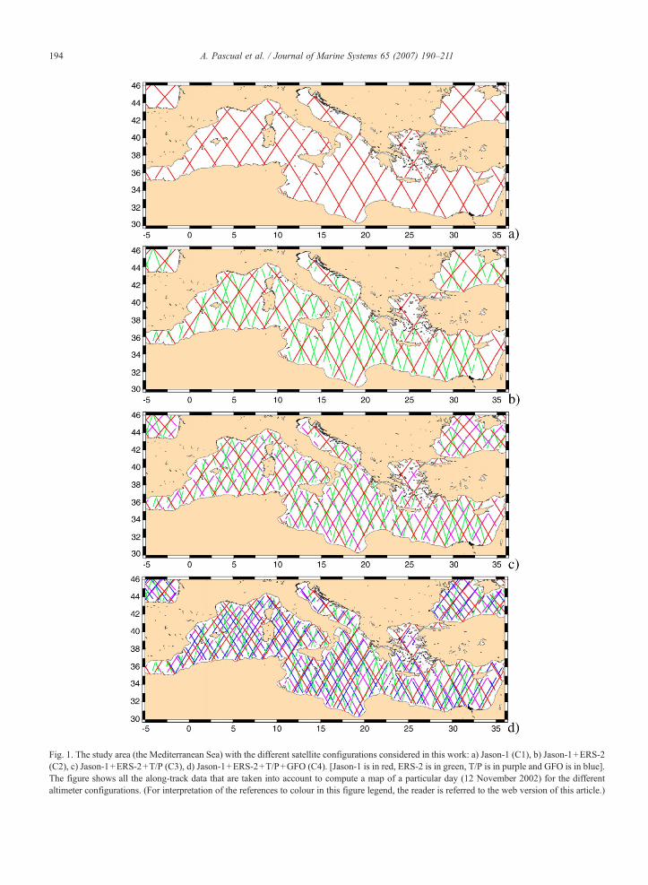
Fig. 1. The study area (the Mediterranean Sea) with the different satellite configurations considered in this work: a) Jason-1 (C1), b) Jason-1+ERS-2(C2), c) Jason-1+ERS-2+T/P (C3), d) Jason-1+ERS-2+T/P+GFO (C4). [Jason-1 is in red, ERS-2 is in green, T/P is in purple and GFO is in blue].The figure shows all the along-track data that are taken into account to compute a map of a particular day (12 November 2002) for the differentaltimeter configurations. (For interpretation of the references to colour in this figure legend, the reader is referred to the web version of this article.)


Fig. 2. Mapping error defined as rms SLA differences between the four-satellite configuration (Jason-1+ERS-2+T/P+GFO, C4) and the otherconfigurations: a) Jason-1 (C1), b) Jason-1+ERS-2 (C2), and c) Jason-1+ERS-2+T/P (C3). Units are cm. (For interpretation of the references tocolour in this figure legend, the reader is referred to the web version of this article.)


with Jason-1 and ENVISAT, it is the most likelyconfiguration to last longer in the future.

Finally, Fig. 2c depicts the averaged mapping errorsfor the three-altimeter configuration (Jason-1+ERS-2+T/P). There is a large impact of introducing T/P since themean rms value is reduced to 1.19 cm rms. The T/Ptracks can be clearly identified and the map is muchhomogeneous than the previous ones, with values al-ways lower than 5 cm. The contribution of GFO (con-tained in the reference four-satellite configuration) is

however not negligible because there are still someareas, especially in the western Alboran sea and Mersa-Mathuh area, where the differences are of about 4.5 cmrms. This means that GFO is really useful and com-plementary for areas of intense mesoscale activity.

3.2. Validation with independent altimetric data

The aim of this section is to carry out a validation ofthe merged maps from a comparison with independent


altimetric data. For this study, we consider GFO along-track data as independent data and we interpolate thecombined maps (that do not use GFO data) along thetime and position of the GFO tracks. Some tests weredone by taking ERS-2 as the independent mission andwe obtained very similar results. The same kind ofvalidation study has been performed very recently by LeTraon and Dibarboure (2004), in order to validate themerging of the Jason-1 and T/P tandem mission, byusing ERS-2 as independent data.

GFO along track data were low-pass filtered using aLanczos filter to retain wavelengths larger than 100 km.Same processing was applied to the SLA data (from thedifferent configuration maps) estimated along GFOtracks. This allows a reduction of altimeter noise whilepreserving most of the mesoscale signal.

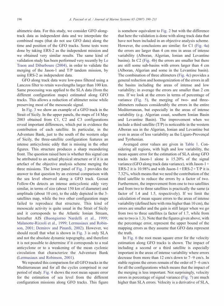
In Fig. 3 we show an example of a GFO track in theStrait of Sicily. In the upper panels, the maps of 14 May2003 obtained from C1, C2 and C3 configurationsreveal important differences, which put in evidence thecontribution of each satellite. In particular, in theAdventure Bank, just to the south of the western edgeof Sicily, the three-satellite configuration features anintense anticyclonic eddy that is missing in the otherfigures. This structure produces a sharp meanderingfront. The question raised here is whether this signal canbe attributed to an actual physical structure or if it is anartefact of the objective analysis scheme merging thethree missions. The lower panel of Fig. 3 provides theanswer to that question by an external comparison withthe sea level observed along a GFO track. GeosatFollow-On detects an intense anticyclonic eddy verysimilar, in terms of size (about 150 km of diameter) andamplitude (about 10 cm), to the eddy depicted in the 3-satellites map, while the two other configuration mapsfailed to reproduce that structure. This kind ofmesoscale activity is quite usual in the Strait of Sicilyand it corresponds to the Atlantic Ionian Stream,hereafter AIS (Buongiorno Nardelli et al., 1999;Malanotte-Rizzoli et al., 1999; Lermusiaux and Robin-son, 2001; Demirov and Pinardi, 2002). However, weshould recall that what is shown in Fig. 3 is only SLAand not the absolute dynamic topography, and thereforeit is not possible to determine if it corresponds to a realanticyclone or to a weakening of the mean cycloniccirculation that characterize the Adventure Bank(Lermusiaux and Robinson, 2001).

We repeated this comparison for all GFO tracks in theMediterranean and for all the cycles comprised in ourperiod of study. Fig. 4 shows the root mean square errorfor the estimation of sea level from the differentconfiguration missions along GFO tracks. This figure

is somehow equivalent to Fig. 2 but with the differencethat here the validation is done with along track data thathave not been included in an objective analysis scheme.However, the conclusions are similar: for C1 (Fig. 4a)the errors are larger than 4 cm rms in areas of intensevariability (Alboran, Algerian, Ionian and Levantinebasins). In C2 (Fig. 4b) the errors are smaller but thereare still some sub-basins with errors larger than 4 cm(Alboran, Algerian and some in the Levantine basin).The combination of three altimeters (Fig. 4c) provides ageneral reduction and homogenization of the errors in allthe basins including the areas of intense and lowvariability; in average the errors are smaller than 2 cmrms. If we look at the errors in terms of percentage ofvariance (Fig. 5), the merging of two- and three-altimeters reduces considerably the errors in the entireMediterranean, but especially in the areas of intensevariability (e.g. Algerian coast, southern Ionian Basinand Levantine Basin). The improvement when weinclude a third satellite (T/P) is noticeable in the westernAlboran sea in the Algerian, Ionian and Levantine buteven in areas of less variability as the Liguro-Provençaland Tyrrhenian.

Averaged error values are given in Table 1. Con-sidering all regions, with high and low variability, themean square error for the estimation of SLA along GFOtracks with Jason-1 alone is 15.20% of the signalvariance (GFO along track data variance), with Jason-1+ERS-2 it is 10.98% and with Jason-1+ERS-2+T/P it is7.32%, which means that we need the contribution of thethird satellite to reduce the errors by a factor of two.Furthermore, the improvement from one to two satellitesand from two to three satellites is practically the same (afactor of 1.4 and 1.5, respectively). If we limit thecalculation of mean square errors to the areas of intensevariability (defined here with rms higher than 10 cm), theerrors are smaller and the gain is still larger when we gofrom two to three satellites (a factor of 1.7, while fromone to two is 1.3). Note that the figures given above, withthe percentage error, represent the upper bound of themapping errors as they assume that GFO data representthe truth.

In Fig. 6 the root mean square error for the velocityestimation along GFO tracks is shown. The impact ofincluding a second or a third satellite is especiallyimportant in the areas of intense variability where errorsdecrease from more than 12 cm/s down to 7–9 cm/s. Instable regions the errors remain of the order of 5–6 cm/sfor all the configurations which means that the impact ofthe merging is less important. Not surprisingly, velocityerrors in percentage of signal variance (Fig. 7) are muchhigher than SLA errors. Velocity is a derivative of SLA,

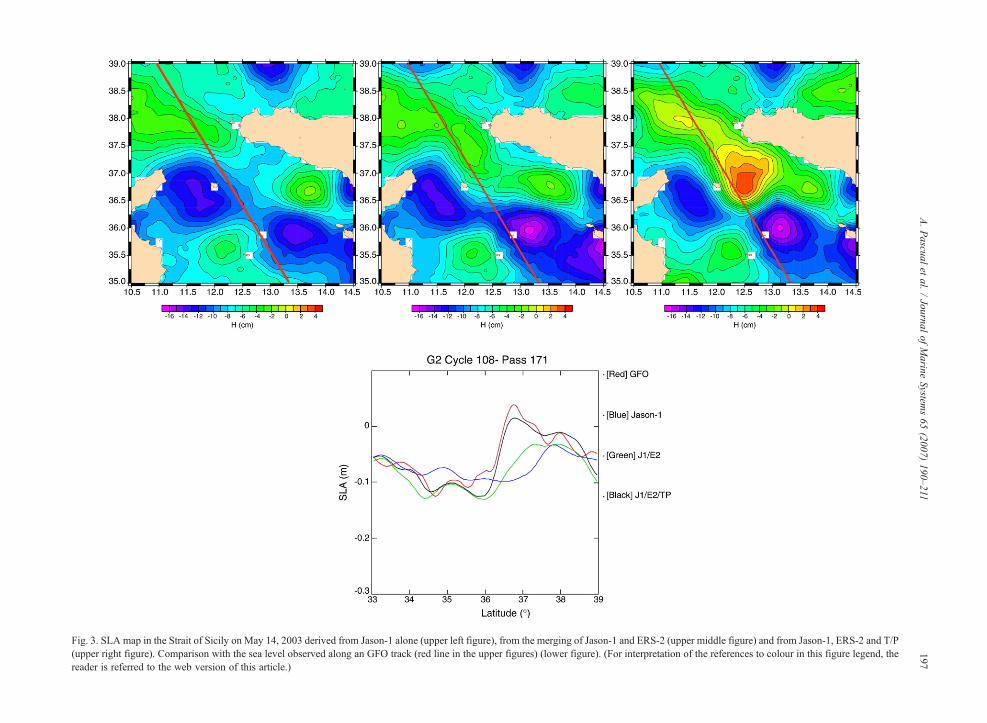
Fig. 3. SLA map in the Strait of Sicily on May 14, 2003 derived from Jason-1 alone (upper left figure), from the merging of Jason-1 and ERS-2 (upper middle figure) and from Jason-1, ERS-2 and T/P(upper right figure). Comparison with the sea level observed along an GFO track (red line in the upper figures) (lower figure). (For interpretation of the references to colour in this figure legend, thereader is referred to the web version of this article.)

197A.Pascual

etal.

/Journal

ofMarine

Systems65

(2007)190–211

Fig. 4. Root mean square error for the estimation of sea level along GFO tracks from the different satellite configurations: a) Jason-1, b) Jason-1+ERS-2, c) Jason-1+ERS-2+T/P. The data have been averaged in square boxes of 1°×1°. Units are cm. (For interpretation of the references to colourin this figure legend, the reader is referred to the web version of this article.)


and velocity mapping is much more demanding in termsof sampling. Again, the errors are larger in stable regionsand smaller in variable areas and they are reduced as thenumber of satellites increases. Errors are reduced by afactor of 1.5 from one to two satellites (choosing onlythe areas of intense variability); from two to threesatellites the reduction is by a factor of 1.2; and in total,from one to three satellites by a factor of 1.8. Le Traonand Dibarboure (2004), considered that to computecross-track velocities, more filtering of SLA data isneeded to reduce the impact of altimeter noise.Therefore, we repeated the computations but by filtering

the along track data at 150 km instead of 100 km, and,obviously, the errors decrease (see Table 2). Thecombination of three satellites (Jason-1+ERS-2+T/P)provides a mean velocity mapping error of only 23%.The relative gain from one to two satellites is now afactor of 1.5, as well as from two to three satellites,which gives a total factor of 2.2, when going from one tothree satellites.

In summary, with the combination of three altimeters,in regions of large mesoscale variability, the sea leveland velocity can be mapped respectively with anaccuracy of about 6% and 23%, which is a factor of

Fig. 5. Mean square error for the estimation of sea level along GFO tracks from the different satellite configurations: a) Jason-1, b) Jason-1+ERS-2, c)Jason-1+ERS-2+T/P. The data have been averaged in square boxes of 1°×1°.Units are% of signal variance. (For interpretation of the references to colourin this figure legend, the reader is referred to the web version of this article.)


2.2 less than the results derived from Jason-1 alone, anda factor of about 1.5 less than the results obtained fromJason-1+ERS-2. Unfortunately, the methodology ap-

Table 1Averaged mean square error for the estimation of sea level along GFOtracks from the different satellite configurations

Altimeter configuration Error (%)

Jason-1 15.20/12.16Jason-1+ERS-2 10.98/9.32Jason-1+ERS-2+T/P 7.32/5.57

The first number corresponds to the average taking into account all thedata and the second one is only considering the areas of intensevariability (rmsN10 cm). Units are % of signal variance.

plied here does not allow validating the four-satelliteconfiguration, because for that purpose a fifth altimeterwould be necessary as independent mission.

Le Traon and Dibarboure (2004) obtained similarresults (about 6% and 20–30% error for sea levelanomaly and velocity estimation, respectively) but fromthe tandem mission, that is by combining only twomissions (Jason-1+T/P). However, Le Traon andDibarboure (2004) defined the areas of intense var-iability as being characterized by rms higher than 20 cmrms. This implies that the entire Mediterranean isneglected, since the variability in the Mediterranean isweaker than 20 cm rms (this is whywe have selected here

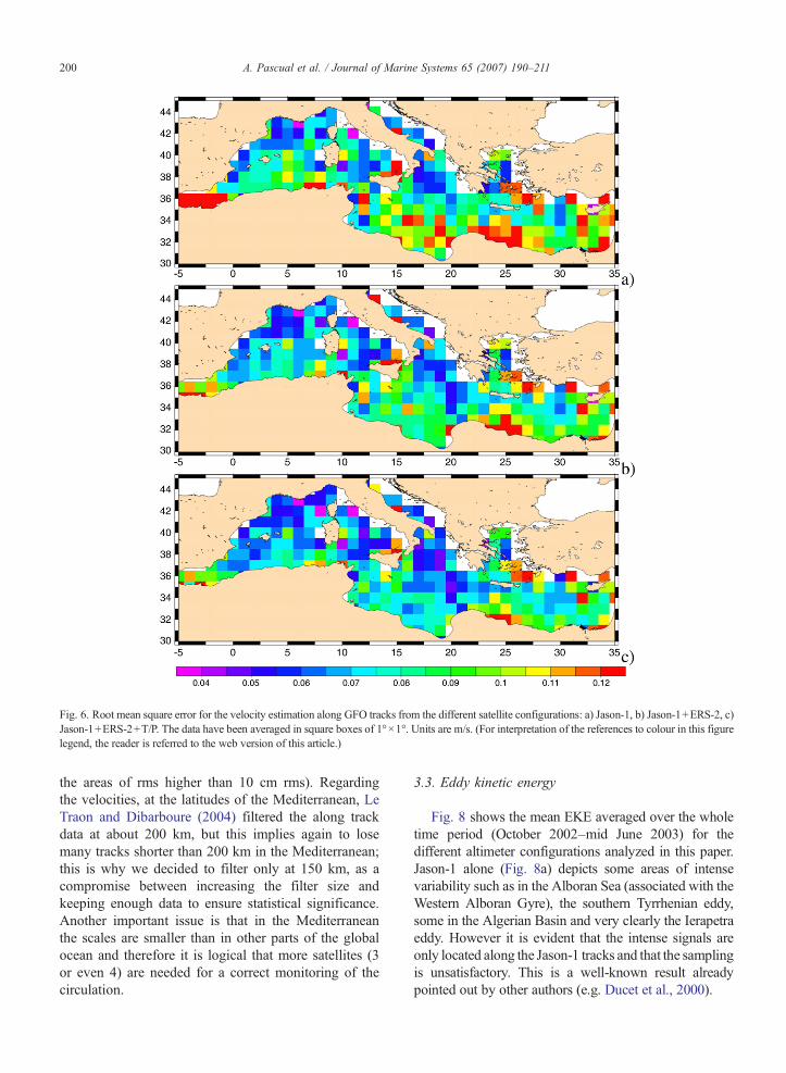
Fig. 6. Root mean square error for the velocity estimation along GFO tracks from the different satellite configurations: a) Jason-1, b) Jason-1+ERS-2, c)Jason-1+ERS-2+T/P. The data have been averaged in square boxes of 1°×1°. Units are m/s. (For interpretation of the references to colour in this figurelegend, the reader is referred to the web version of this article.)


the areas of rms higher than 10 cm rms). Regardingthe velocities, at the latitudes of the Mediterranean, LeTraon and Dibarboure (2004) filtered the along trackdata at about 200 km, but this implies again to losemany tracks shorter than 200 km in the Mediterranean;this is why we decided to filter only at 150 km, as acompromise between increasing the filter size andkeeping enough data to ensure statistical significance.Another important issue is that in the Mediterraneanthe scales are smaller than in other parts of the globalocean and therefore it is logical that more satellites (3or even 4) are needed for a correct monitoring of thecirculation.

3.3. Eddy kinetic energy

Fig. 8 shows the mean EKE averaged over the wholetime period (October 2002–mid June 2003) for thedifferent altimeter configurations analyzed in this paper.Jason-1 alone (Fig. 8a) depicts some areas of intensevariability such as in the Alboran Sea (associated with theWestern Alboran Gyre), the southern Tyrrhenian eddy,some in the Algerian Basin and very clearly the Ierapetraeddy. However it is evident that the intense signals areonly located along the Jason-1 tracks and that the samplingis unsatisfactory. This is a well-known result alreadypointed out by other authors (e.g. Ducet et al., 2000).

Fig. 7. Mean square error for the velocity estimation along GFO tracks from the different satellite configurations: a) Jason-1, b) Jason-1+ERS-2, c)Jason-1+ERS-2+T/P. The data have been averaged in square boxes of 1°×1°. Units are % of signal variance. (For interpretation of the references tocolour in this figure legend, the reader is referred to the web version of this article.)


A clear improvement is obtained with the mean EKEfor Jason-1+ERS-2 configuration (Fig. 8b). In essence,there is a more clear continuity in all the features ofEKE. In the western Mediterranean sea, the variability ofboth western and eastern Alboran gyres is better re-produced as well as the Algerian eddies that are formedbetween 5°E and 10°E. On the other hand, in the IonianBasin the differences are important since the AIS can benow identified linking the Ionian and theLevantine basins,associated with some mesoscale activity. Southwest ofPeloponnese there is a weak signal that corresponds to thePelops anticyclone (Hamad et al., 2005). Finally in theLevantine basin, the most important feature is the

Schikmona gyre (centred at ∼34°E and ∼33.5°N) thatwas clearly undersampled in the Jason-1 map.

However, Fig. 8b still presents some deficiencies.For instance, along the Libyan coast, just south ofIerapetra, there is a gap in an energetic area identified asthe Mersa-Matruth gyre (e.g. Iudicone et al., 1998). Thecombination of three satellites (Jason-1+ERS-2+T/P,Fig. 8c) confirms that this area (between 26°E and27.5°E) is characterized by an intense variability (meanEKE ∼250 cm2/s2) which is missed by the combinationof Jason-1+ERS-2 due to the poor sampling. Fig. 9shows an example of an intense anticyclonic eddy pre-sent in that area (as revealed by the SST pattern) that is

Table 2Averaged mean square error for the velocity estimation along GFOtracks from the different satellite configurations

Altimeter configuration Error (%)

Jason-1 66.37/51.11Jason-1+ERS-2 43.42/34.09Jason-1+ERS-2+T/P 36.45/22.95

The first number corresponds to the result when the data are filtered at100 km and the second one with the data filtered at 150 km. Only areasof intense variability (rmsN15 cm/s) have been considered. Units are% of signal variance.


almost missed by the two-satellite configuration but thatis much better reproduced when we include the thirdsatellite. In fact, this area has been recently defined(Larnicol et al., 2002; Hamad et al., 2005) as a preferredsite for the propagation and interaction of anticycloniceddies instead of being occupied by a single well-defined gyre. This is in agreement with our resultsbecause the Mersa-Matruth place appears more like theAlgerian Basin with intense patches of EKE all alongthe coast, in contrast to the Ierapetra and Schikmonagyres that can be clearly identified as gyre structureswith maximum EKE on the perimeter of the gyres andlow energy in the center.

Similarly, in the Western Basin, between Minorcaand Sardinia islands, the two-mission configuration isnot able to capture some of the signal that is char-acteristic of Algerian eddies detaching from the Al-gerian coast and propagating more to the North (Puillatet al., 2002). These spots are detected by the combi-nation of Jason-1+ERS-2+T/P. In the Ionian Basin, theAIS is more intense and the region of higher energy isalmost continuous (Fig. 8c).

On the contrary, along the Algerian coast, between0°E and 2.5°E, in the two-altimeter configuration there isan area of very low energy that corresponds to an area ofhigh error mapping (see Fig. 2b). The combination ofthree satellites (Fig. 8c) adds some energy but the EKElevel is not as intense as it is between 5°E and 10°E(Fig. 8c). This may indicate that the Algerian Current isquite stable in this area and that, in fact, the combinationof two satellites was not underestimating a significantportion of energy in that zone, at least during the periodof time that is studied here.

Finally, the differences between three- and four-al-timeter configurations are not very large but not negligible.In general, the fourth altimeter (GFO) contributes to theintensification of all the structures (Alboran, see the zoomin Fig. 10, Algerian eddies; a second branch of the AISmore to the south flowing along the Libyan coast at about15°E parallel to the bathymetry; some more energy in theMersa-Matruth area as well as in the Shikmona gyre).

A major conclusion is that the combination of severalaltimeters has not introduced noise in areas of lowvariability, such as the Northwestern Basin where thevariability remains weak for all the configurations; on thecontrary, the EKE has been only gained in zones that areknown to be energetic. This proves that the merging hasbeen successful.

The spatial mean is complementary to the temporalmean as it provides the temporal evolution of EKE(Fig. 11). For all configurations we observe a seasonalcycle being maximum in winter (end of January). Thisseems to correspond to the ocean response to the annualcycle of the wind stress, at least for a global scale(Stammer and Wunsch, 1999; Ducet et al., 2000). Forthe Mediterranean, the same hypotheses have beenmade and have been illustrated with modelling studies(Demirov and Pinardi, 2002; Molcard et al., 2002). Inparticular, the seasonal cycle observed in the EKEprobably corresponds to the variability of the mesoscaleactivity and also to the intensification of the generalMediterranean circulation in winter. However, thecauses of the EKE seasonality are beyond the scope ofthis work. We want to focus on the level of energy givenby the different altimeter configurations. While themean EKE for C1 is only 70.3 cm2/s2, it is 98.9 cm2/s2

for C2. This implies that the merged Jason-1+ERS-2maps yield EKE levels 40% higher than Jason-1 alone.For the global ocean, Ducet et al. (2000) found that theimpact of introducing ERS-2 signified an increase inEKE of 30%, a value slightly smaller than the oneobtained in this work, which shows that ERS-2 isessential to reproduce the relatively small structures thatcharacterize the Mediterranean. The differences be-tween two- and three-satellite configurations are smaller(mean EKE for C3 is 108.7 cm2/s2), but it still repre-sents a gain of 10% with respect to the two-satellitecombination. Finally, the contribution of the fourth sa-tellite (GFO) gives a mean EKE in C4 of 113.57 cm2/s2,i.e. 5% larger than C3. Therefore, the four-altimeterconfiguration provides a mean EKE 15% higher than thereference configuration (Jason-1+ERS-2).

3.4. Comparison with other data

In this last section we compare altimetric data with SeaSurface Temperature (SST), tide gauges and drifters withthe aim of having other independent data sets to validateand verify to what extent we are able to reproduce themesoscale in the Mediterranean with four altimeters. Thecomparison between altimetry and SST/lagrangian buoyscannot be achieved unless a Mean Dynamic Topography(MDT) is added to the SLA to get absolute values of the

Fig. 8. Mean EKE averaged over the period of study (October 2002–June 2003) for the different satellite configurations as marked in Fig. 1. Units arecm2/s2. (For interpretation of the references to colour in this figure legend, the reader is referred to the web version of this article.)


Fig. 9. Example of an eddy in the Levantine basin that is not properly detected by the 2-satellite configuration. Left panel: SST image for 13 June 2003 (CMS), where the marked rectangle correspondsto the area shown in the other two panels. Middle panel: SLA of 11 June 2003 for the Jason-1+ERS-2 configuration. Right panel: SLA of 11 June 2003 for the Jason-1+ERS-2+T/P+GFOconfiguration. Units in SST image are K and in SLA maps are cm. (For interpretation of the references to colour in this figure legend, the reader is referred to the web version of this article.)

204A.Pascual

etal.

/Journal

ofMarine

Systems65

(2007)190–211

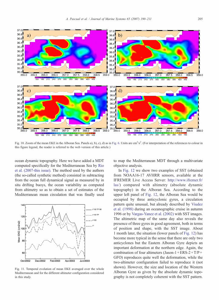
Fig. 10. Zoom of the mean EKE in the Alboran Sea. Panels a), b), c), d) as in Fig. 6. Units are cm2/s2. (For interpretation of the references to colour inthis figure legend, the reader is referred to the web version of this article.)


ocean dynamic topography. Here we have added a MDTcomputed specifically for the Mediterranean Sea by Rioet al. (2007-this issue). The method used by the authors(the so-called synthetic method) consisted in subtractingfrom the ocean full dynamical signal as measured by insitu drifting buoys, the ocean variability as computedfrom altimetry so as to obtain a set of estimates of theMediterranean mean circulation that was finally used

Fig. 11. Temporal evolution of mean EKE averaged over the wholeMediterranean and for the different altimeter configuration consideredin this study.

to map the Mediterranean MDT through a multivariateobjective analysis.

In Fig. 12 we show two examples of SST (obtainedfrom NOAA16-17 AVHRR sensors, available at theIFREMER Live Access Server: http://www.ifremer.fr/las/) compared with altimetry (absolute dynamictopography) in the Alboran Sea. According to theupper left panel of Fig. 12, the Alboran Sea would beoccupied by three anticyclonic gyres, a circulationpattern quite unusual, but already described by Viudezet al. (1998) during an oceanographic cruise in autumn1996 or by Vargas-Yanez et al. (2002) with SST images.The altimetric map of the same day also reveals thepresence of three gyres in good agreement, both in termsof position and shape, with the SST image. About1 month later, the situation (lower panels of Fig. 12) hasbecome more typical in the sense that there are only twoanticyclones but the Eastern Alboran Gyre depicts animportant deformation at the northern edge. Again, thecombination of four altimeters (Jason-1+ERS-2+T/P+GFO) reproduces quite well the deformation, while thetwo-altimeter configuration failed to reproduce it (notshown). However, the size and location of the WesternAlboran Gyre as given by the absolute dynamic topo-graphy is not completely coherent with the SST pattern.

http://www.ifremer.fr/las/

http://www.ifremer.fr/las/

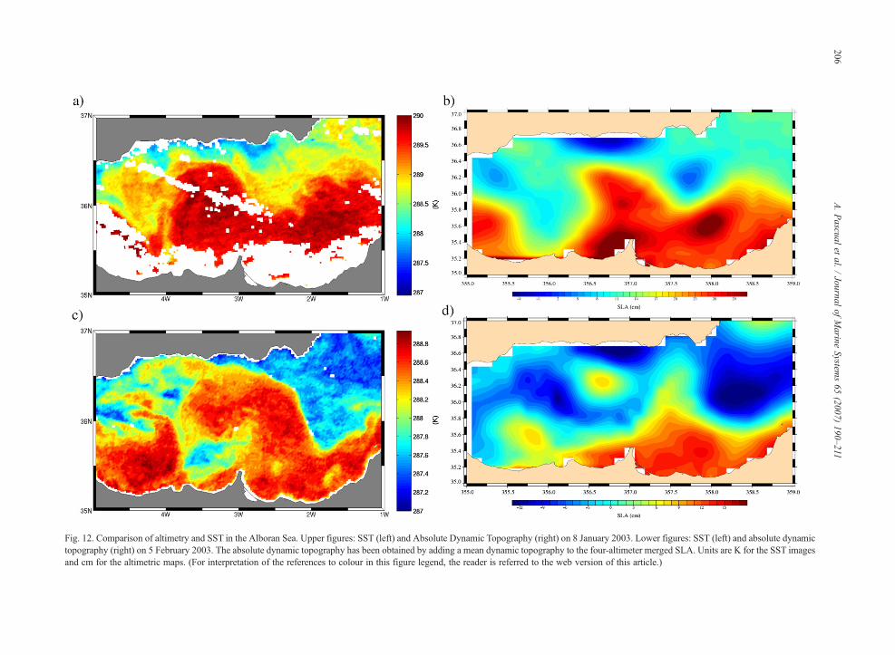
Fig. 12. Comparison of altimetry and SST in the Alboran Sea. Upper figures: SST (left) and Absolute Dynamic Topography (right) on 8 January 2003. Lower figures: SST (left) and absolute dynamictopography (right) on 5 February 2003. The absolute dynamic topography has been obtained by adding a mean dynamic topography to the four-altimeter merged SLA. Units are K for the SST imagesand cm for the altimetric maps. (For interpretation of the references to colour in this figure legend, the reader is referred to the web version of this article.)

206A.Pascual

etal.

/Journal

ofMarine

Systems65

(2007)190–211

Fig. 13. Comparison of altimetry and SST in the Algerian Basin. Upper figures: SST (left) and Absolute Dynamic Topography (right) on 15 May2003. Lower figures: SST (left) and Absolute Dynamic Topography (right) on 21 May 2003. The absolute dynamic topography has been obtained byadding a mean dynamic topography to the four-altimeter merged SLA. Units are K for the SST images and cm for the altimetric maps. (Forinterpretation of the references to colour in this figure legend, the reader is referred to the web version of this article.)


Another example of SST versus altimetry is shown inFig. 13 for the Algerian Basin. Between Sardinia and theBalearic Islands, the SST image displays (upper leftpanel) some structures that are also identified in thealtimetry field (upper right panel): a filament of warmwater with an anticyclonic curvature centred at about5°E and 41°N, an intense cyclonic eddy located to theeast of the anticyclonic filament, and, finally, south ofthese features, two anticyclonic eddies that are somehowlinked. All these features are in agreement with theabsolute dynamic topography pattern. Just 1 week later,

the outstanding feature is that the two anticyclones thatwere linked are separated by a tongue of relatively coldwater. The altimetric map also reveals the same change,the two eddies are not linked any more. We consider thatthis is a nice example illustrating how the merging offour altimeters improves not only the description of themesoscale in the spatial domain but also in the temporaldomain, since changes that take place in the scale of aweek are properly detected.

Surface drifters also provide valuable information tobe compared with altimetry. The drifting buoy data used

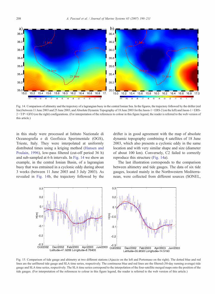
Fig. 14. Comparison of altimetry and the trajectory of a lagrangian buoy in the central Ionian Sea. In the figures, the trajectory followed by the drifter (redline) between 11 June 2003 and 25 June 2003, andAbsoluteDynamicTopography of 18 June 2003 for the Jason-1+ERS-2 (on the left) and Jason-1+ERS-2+T/P+GFO (on the right) configurations. (For interpretation of the references to colour in this figure legend, the reader is referred to the web version ofthis article.)


in this study were processed at Istituto Nazionale diOceanografia e di Geofisica Sperimentale (OGS),Trieste, Italy. They were interpolated at uniformlydistributed times using a kriging method (Hansen andPoulain, 1996), low-pass filtered (cut-off period 36 h)and sub-sampled at 6-h intervals. In Fig. 14 we show anexample, in the central Ionian Basin, of a lagrangianbuoy that was entrained in a cyclonic eddy during about3 weeks (between 11 June 2003 and 3 July 2003). Asrevealed in Fig. 14b, the trajectory followed by the

Fig. 15. Comparison of tide gauge and altimetry at two different stations (Ajlines are the unfiltered tide gauge and SLA time series, respectively. The congauge and SLA time series, respectively. The SLA time series correspond to thtide gauges. (For interpretation of the references to colour in this figure lege

drifter is in good agreement with the map of absolutedynamic topography combining 4 satellites of 18 June2003, which also presents a cyclonic eddy in the samelocation and with very similar shape and size (diameterof about 100 km). Conversely, C2 failed to correctlyreproduce this structure (Fig. 14a).

The last illustration corresponds to the comparisonbetween altimetry and tide gauges. The data of six tidegauges, located mainly in the Northwestern Mediterra-nean, were collected from different sources (SONEL,

accio on the left and Portomaso on the right). The dotted blue and redtinuous blue and red lines are the filtered (30-day running average) tidee interpolation of the four-satellite merged maps onto the position of thend, the reader is referred to the web version of this article.)

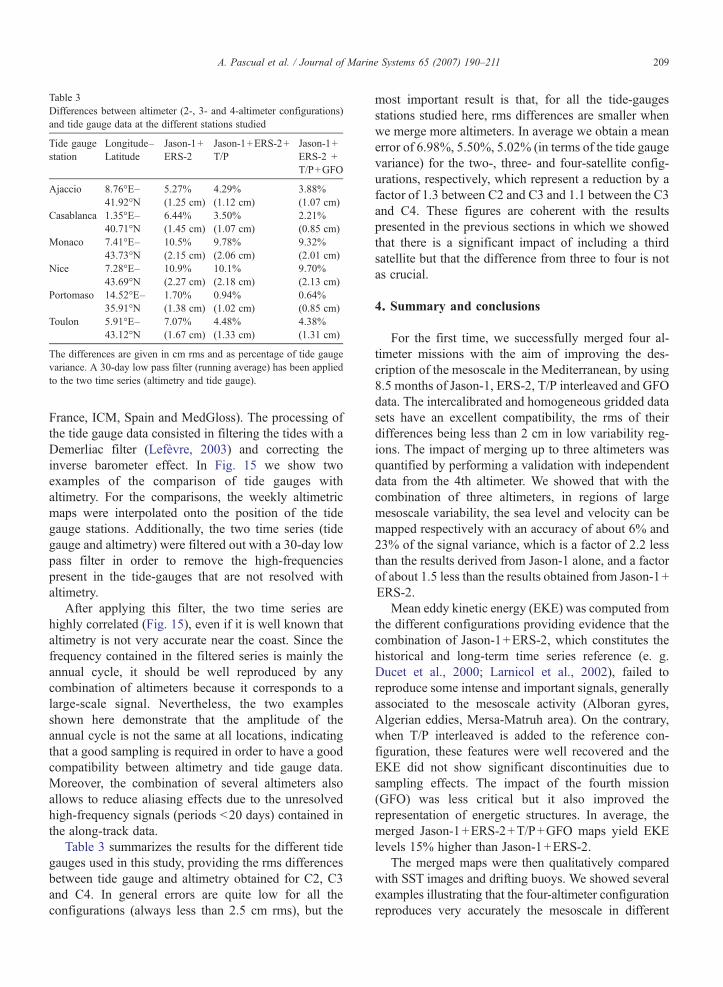
Table 3Differences between altimeter (2-, 3- and 4-altimeter configurations)and tide gauge data at the different stations studied

Tide gaugestation

Longitude–Latitude

Jason-1+ERS-2

Jason-1+ERS-2+T/P

Jason-1+ERS-2 +T/P+GFO

Ajaccio 8.76°E–41.92°N

5.27%(1.25 cm)

4.29%(1.12 cm)

3.88%(1.07 cm)

Casablanca 1.35°E–40.71°N

6.44%(1.45 cm)

3.50%(1.07 cm)

2.21%(0.85 cm)

Monaco 7.41°E–43.73°N

10.5%(2.15 cm)

9.78%(2.06 cm)

9.32%(2.01 cm)

Nice 7.28°E–43.69°N

10.9%(2.27 cm)

10.1%(2.18 cm)

9.70%(2.13 cm)

Portomaso 14.52°E–35.91°N

1.70%(1.38 cm)

0.94%(1.02 cm)

0.64%(0.85 cm)

Toulon 5.91°E–43.12°N

7.07%(1.67 cm)

4.48%(1.33 cm)

4.38%(1.31 cm)

The differences are given in cm rms and as percentage of tide gaugevariance. A 30-day low pass filter (running average) has been appliedto the two time series (altimetry and tide gauge).


France, ICM, Spain and MedGloss). The processing ofthe tide gauge data consisted in filtering the tides with aDemerliac filter (Lefèvre, 2003) and correcting theinverse barometer effect. In Fig. 15 we show twoexamples of the comparison of tide gauges withaltimetry. For the comparisons, the weekly altimetricmaps were interpolated onto the position of the tidegauge stations. Additionally, the two time series (tidegauge and altimetry) were filtered out with a 30-day lowpass filter in order to remove the high-frequenciespresent in the tide-gauges that are not resolved withaltimetry.

After applying this filter, the two time series arehighly correlated (Fig. 15), even if it is well known thataltimetry is not very accurate near the coast. Since thefrequency contained in the filtered series is mainly theannual cycle, it should be well reproduced by anycombination of altimeters because it corresponds to alarge-scale signal. Nevertheless, the two examplesshown here demonstrate that the amplitude of theannual cycle is not the same at all locations, indicatingthat a good sampling is required in order to have a goodcompatibility between altimetry and tide gauge data.Moreover, the combination of several altimeters alsoallows to reduce aliasing effects due to the unresolvedhigh-frequency signals (periods b20 days) contained inthe along-track data.

Table 3 summarizes the results for the different tidegauges used in this study, providing the rms differencesbetween tide gauge and altimetry obtained for C2, C3and C4. In general errors are quite low for all theconfigurations (always less than 2.5 cm rms), but the

most important result is that, for all the tide-gaugesstations studied here, rms differences are smaller whenwe merge more altimeters. In average we obtain a meanerror of 6.98%, 5.50%, 5.02% (in terms of the tide gaugevariance) for the two-, three- and four-satellite config-urations, respectively, which represent a reduction by afactor of 1.3 between C2 and C3 and 1.1 between the C3and C4. These figures are coherent with the resultspresented in the previous sections in which we showedthat there is a significant impact of including a thirdsatellite but that the difference from three to four is notas crucial.

4. Summary and conclusions

For the first time, we successfully merged four al-timeter missions with the aim of improving the des-cription of the mesoscale in the Mediterranean, by using8.5 months of Jason-1, ERS-2, T/P interleaved and GFOdata. The intercalibrated and homogeneous gridded datasets have an excellent compatibility, the rms of theirdifferences being less than 2 cm in low variability reg-ions. The impact of merging up to three altimeters wasquantified by performing a validation with independentdata from the 4th altimeter. We showed that with thecombination of three altimeters, in regions of largemesoscale variability, the sea level and velocity can bemapped respectively with an accuracy of about 6% and23% of the signal variance, which is a factor of 2.2 lessthan the results derived from Jason-1 alone, and a factorof about 1.5 less than the results obtained from Jason-1+ERS-2.

Mean eddy kinetic energy (EKE) was computed fromthe different configurations providing evidence that thecombination of Jason-1+ERS-2, which constitutes thehistorical and long-term time series reference (e. g.Ducet et al., 2000; Larnicol et al., 2002), failed toreproduce some intense and important signals, generallyassociated to the mesoscale activity (Alboran gyres,Algerian eddies, Mersa-Matruh area). On the contrary,when T/P interleaved is added to the reference con-figuration, these features were well recovered and theEKE did not show significant discontinuities due tosampling effects. The impact of the fourth mission(GFO) was less critical but it also improved therepresentation of energetic structures. In average, themerged Jason-1+ERS-2+T/P+GFO maps yield EKElevels 15% higher than Jason-1+ERS-2.

The merged maps were then qualitatively comparedwith SST images and drifting buoys. We showed severalexamples illustrating that the four-altimeter configurationreproduces very accurately the mesoscale in different


regions of the Mediterranean (Alboran Sea, Algerian,Ionian and Levantine Basins), improving the descriptiongiven by the combination of only two altimeters. Aquantitative comparison between altimetry and tide gaugedata (from stations located in the North WesternMediterranean) has proved the high compatibility be-tween both data sets and that the errors are reduced by afactor of 1.3 when we combined four missions withrespect to the two-mission configuration.

Based on these results, at least three altimeters areneeded for a correct monitoring of the mesoscale circu-lation in the Mediterranean Sea. In any case, the opti-mized tandem mission Jason-1+T/P interleaved ispreferable than the Jason-1+ERS-2 configuration. Ourresults are in good agreement with those obtained intheoretical studies (Le Traon and Dibarboure, 1999; LeTraon et al., 2001; Le Traon and Dibarboure, 2002) inthe sense that the contribution of a third and a fourthaltimeter is less critical than just a second one. However,we have shown that in the Mediterranean the impact ofthe third and fourth altimeters would be higher than inother parts of the ocean, probably due to the typical sizeof the structures that are not correctly sampled by theJason-1+ERS-2 configuration. Future studies shouldbe carried out over the global ocean, by using alsoENVISAT data and a longer time series.

Acknowledgements

Ananda Pascual acknowledges a Marie Curie HostIndustry Fellowship funded by the European Commis-sion (Fellowship Contract: HPMI-CT-2001-00100). Thealtimeter products were produced by SSALTO/DUACSas part of the Environment and Climate European Enactproject (EVK2-CT2001-00117) and distributed byAVISO, with support from CNES. The drifting buoydata were kindly provided by Pierre-Marie Poulain fromOGS, Italy.

References

Ayoub, N., Le Traon, P.-Y., De Mey, P., 1998. A description of theMediterranean surface variable circulation from combined ERS-1and TOPEX/POSEIDON altimetric data. J. Mar. Syst. 18 (1–3),3–40.

Bretherton, F., Davis, R., Fandry, C., 1976. A technique for objectiveanalysis and design of oceanographic experiments applied toMODE-3. Deep-Sea Res. 23, 559–582.

Buongiorno Nardelli, B., Santoleri, R., Zoffoli, S., Marullo, S., 1999.Altimetric signal and three-dimensional structure of the sea in theChannel of Sicily. J. Geophys. Res. 104 (C9), 20585–20603.

Chelton, D.B., Schlax, M.G., 2003. The accuracies of smoothed seasurface height fields constructed from tandem satellite altimeterdatasets. J. Atmos. Ocean. Technol. 20, 1276–1302.

Demirov, E., Pinardi, N., 2002. Simulation of the Mediterranean Seacirculation from 1979 to 1993: Part I. The interannual variability.J. Mar. Syst. 33–34, 23–50.

Ducet, N., Le Traon, P.Y., 2001. A comparison of surface eddy kineticenergy and Reynold stresses in the Gulf Stream and the KuroshioCurrent systems from merged TOPEX/Poseidon and ERS-1/2altimetric data. J. Geophys. Res. 106 (C8), 16603–16622.

Ducet, N., Le Traon, P.Y., Reverdin, G., 2000. Global high resolutionmapping of ocean circulation from the combination of TOPEX/POSEIDON and ERS-1/2. J. Geophys. Res. 105 (C8), 19477–19498.

Fu, L.L., Stammer, D., Leben, B.B., Chelton, D.B., 2003. Improvedspatial resolution of ocean surface topography from the TOPEX/Poseidon – Jason-1 tandem altimeter mission. EOS 84 (26),247–248 (241).

Greenslade, D.J.M., Chelton, D.B., Schlax, M.G., 1997. The mid-latitude resolution capability of sea level fields constructed fromsingle and multiple satellite altimeter datasets. J. Atmos. Ocean.Technol. 14, 849–870.

Hamad, N., Millot, C., Taupier-Letage, I., 2005. A new hypothesisabout the surface circulation in the eastern basin of the medi-terranean sea. Prog. Oceanogr. 66 (2–4), 287–298.

Hansen, D.V., Poulain, P.-M., 1996. Quality control and interpolationof WOCE/TOGA drifter data. J. Atmos. Ocean. Technol. 13 (4),900–909.

Iudicone, D., Santoleri, R., Marullo, S., Gerosa, P., 1998. Sea levelvariability and surface eddy statistics in the Mediterranean Seafrom TOPEX/POSEIDON data. J. Geophys. Res. 103 (C2),2995–3012. doi:10.1029/97JC01577.

Koblinsky, C.J., Gaspar, P., Lagerloef, G., 1992. The future ofspaceborne altimetry. Oceans and Climate Change, Joint Ocean-ographic Institutions Incorporated, Washington, D.C. 75 pp.

Larnicol, G., Le Traon, P.-Y., Ayoub, N., De Mey, P., 1995. Mean sealevel and surface circulation variability of the Mediterranean Seafrom 2 years of TOPEX/POSEIDON altimetry. J. Geophys. Res.100, 25163–25177.

Larnicol, G., Ayoub, N., Le Traon, P.-Y., 2002. Major changes inMediterranean Sea level variability from 7 years of TOPEX/POSEIDON and ERS-1/2 data. J. Mar. Syst.: 33–34, 63–89.

Lefèvre, F., 2003. Determination of instantaneous sea level on NWMediterranean Sea for RA-2 absolute calibration long term driftdetermination. Final Report. CLS, Ramonville Saint-Agne, p. 43.

Lermusiaux, P.F.J., Robinson, A.R., 2001. Features of dominantmesoscale variability, circulation patterns and dynamics in the Straitof Sicily. Deep-Sea Res., Part 1, Oceanogr. Res. Pap. 48, 1953–1997.

Leeuwenburgh, Stammer, 2002. Uncertainties in altimetry-basedvelocity estimates. J. Geophys. Res. 107 (10), 3175. doi:10.1029/2001JC000937.

Le Traon, P.Y., Dibarboure, G., 1999. Mesoscale mapping capabilitiesof multiple-satellite altimeter missions. J. Atmos. Ocean. Technol.169, 1208–1223.

Le Traon, P.Y., Dibarboure, G., 2002. Velocity mapping capabilities ofpresent and future altimeter missions: the role of high frequencysignals. J. Atmos. Ocean. Technol. 19, 2077–2088.

Le Traon, P.Y., Dibarboure, G., 2004. An illustration of the uniquecontribution of the TOPEX/Poseidon – Jason-1 tandem mission tomesoscale variability studies. Mar. Geod. 27, 3–13.

Le Traon, P.Y., Ogor, F., 1998. ERS-1/2 orbit improvement usingTOPEX/POSEIDON: the 2 cm challenge. J. Geophys. Res. 103,8045–8057.

Le Traon, P.Y., Ducet, N., Dibarboure, G., 2001. Use of a high-resolution model to analyze the mapping capabilities of multiple-altimeter missions. J. Atmos. Ocean. Technol. 18, 1277–1288.

http://dx.doi.org/10.1029/2001JC000937

http://dx.doi.org/10.1029/97JC01577


Le Traon, P.Y., Faugère, Y., Hernandez, F., Dorandeu, J., Mertz, F.,Ablain, M., 2003. Can we merge GEOSAT Follow-On withTOPEX/POSEIDON and ERS-2 for an improved description ofthe ocean circulation? J. Atmos. Ocean. Technol. 20, 889–895.

Malanotte-Rizzoli, P.,Manca, B.B., Ribera d'Alcala,M., Theocharis, A.,Brenner, S., Budillon, G., Özsoy, E., 1999. The Eastern Mediterra-nean in the 80s and in the 90s: the big transition in the intermediateand deep circulations. Dyn. Atm. Ocean 29, 365–395.

Molcard, A., Pinardi, N., Iskandarani, M., Haidvogel, D.B., 2002.Wind driven general circulation of the Mediterranean Sea sim-ulated with a Spectral Element OceanModel. Dyn. Atm. Ocean 35,97–130.

Puillat, I., Taupier-Letage, I., Millot, C., 2002. Algerian eddies lifetimecan near 3 years. J. Mar. Syst. 31 (4), 245–259.

Pujol, M.-I., Larnicol, G., 2005. Mediterranean sea eddy kinetic energyvariability from 11 years of altimetric data. J. Mar. Syst. 58,121–142.

Rio, M.H., Poulain, P.M., Pascual, A., Mauri, E., Larnicol, G., 2007. Amean dynamic topography of the Mediterranean Sea computedfrom altimetric data and in-situ measurements. J. Mar. Syst. 65,484–508 (this issue). doi:10.1016/j.jmarsys.2005.02.006.

Stammer, D.,Wunsch, C., 1999. Temporal changes in eddy energy of theoceans. Deep-Sea Res., Part 2, Top. Stud. Oceanogr. 46, 77–108.

Tai, C.K., 1998. On the spectral ranges that are resolved by a singlesatellite in exact repeat sampling configuration. J. Atmos. Ocean.Technol. 15, 1459–1470.

Vargas-Yanez,M., Plaza, F., Garcia-Lafuente, J., Sarhan, T., Vargas, J.M.,Velez-Belchi, P., 2002. About the seasonal variability of the AlboranSea circulation. J. Mar. Syst. 35, 229–248.

Vignudelli, S., 1997a. Analysis of ERS-1 altimeter collinear passes inthe Mediterranean Sea during 1992–1993. Int. J. Remote Sens. 18(3), 573–601.

Vignudelli, S., 1997b. Potential use of ERS-1 and TOPEX/Poseidonaltimeters for resolving oceanographic patterns in the AlgerianBasin. Geophys. Res. Lett. 24 (14), 1787–1790. doi:10.1029/97GL01546.

Viudez, A., Pinot, J.M., Haney, R.L., 1998. On the upper layer circulationin the Alboran Sea. J. Geophys. Res. 103 (C10), 21653–21666.

http://dx.doi.org/10.1016/j.jmarsys.2005.02.006

http://dx.doi.org/10.1029/97GL01546

mesoscale mapping capabilities of multisatellite altimeter missions: first results with real data in...

Documents