medslik-ii, a lagrangian marine surface oil spill model for … · 2016-01-24 · conceptual...

Geosci. Model Dev., 6, 1851–1869, 2013www.geosci-model-dev.net/6/1851/2013/doi:10.5194/gmd-6-1851-2013© Author(s) 2013. CC Attribution 3.0 License.

GeoscientificModel Development

Open A

ccess

MEDSLIK-II, a Lagrangian marine surface oil spill model forshort-term forecasting – Part 1: Theory

M. De Dominicis1, N. Pinardi2, G. Zodiatis3, and R. Lardner3

1Istituto Nazionale di Geofisica e Vulcanologia, Bologna, Italy2Corso di Scienze Ambientali, University of Bologna, Ravenna, Italy3Oceanography Centre, University of Cyprus, Nicosia, Cyprus

Correspondence to:M. De Dominicis ([email protected])

Received: 25 January 2013 – Published in Geosci. Model Dev. Discuss.: 8 March 2013Revised: 12 July 2013 – Accepted: 17 July 2013 – Published: 1 November 2013

Abstract. The processes of transport, diffusion and transfor-mation of surface oil in seawater can be simulated using aLagrangian model formalism coupled with Eulerian circu-lation models. This paper describes the formalism and theconceptual assumptions of a Lagrangian marine surface oilslick numerical model and rewrites the constitutive equationsin a modern mathematical framework. The Lagrangian nu-merical representation of the oil slick requires three differentstate variables: the slick, the particle and the structural statevariables. Transformation processes (evaporation, spreading,dispersion and coastal adhesion) act on the slick state vari-ables, while particle variables are used to model the transportand diffusion processes. The slick and particle variables arerecombined together to compute the oil concentration in wa-ter, a structural state variable. The mathematical and numer-ical formulation of oil transport, diffusion and transforma-tion processes described in this paper, together with the manysimplifying hypothesis and parameterizations, form the basisof a new, open source Lagrangian surface oil spill model, theso-called MEDSLIK-II, based on its precursor MEDSLIK(Lardner et al., 1998, 2006; Zodiatis et al., 2008a). Part 2of this paper describes the applications of the model to oilspill simulations that allow the validation of the model re-sults and the study of the sensitivity of the simulated oil slickto different model numerical parameterizations.

1 Introduction

Representing the transport and fate of an oil slick at the seasurface is a formidable task. Many factors affect the motionand transformation of the slick. The most relevant of these

are the meteorological and marine conditions at the air–seainterface (wind, waves and water temperature); the chemicalcharacteristics of the oil; its initial volume and release rates;and, finally, the marine currents at different space scales andtimescales. All these factors are interrelated and must be con-sidered together to arrive at an accurate numerical represen-tation of oil evolution and movement in seawater.

Oil spill numerical modelling started in the early eight-ies and, according to state-of-the-art reviews (ASCE, 1996;Reed et al., 1999), a large number of numerical Lagrangiansurface oil spill models now exist that are capable of sim-ulating three-dimensional oil transport and fate processes atthe surface. However, the analytical and discrete formalismto represent all processes of transport, diffusion and trans-formation for a Lagrangian surface oil spill model are notadequately described in the literature. An overall frameworkfor the Lagrangian numerical representation of oil slicks atsea is lacking and this paper tries to fill this gap.

Over the years, Lagrangian numerical models have de-veloped complex representations of the relevant processes:starting from two-dimensional point source particle-trackingmodels such as TESEO-PICHI (Castanedo et al., 2006;Sotillo et al., 2008), we arrive at complex oil slick polygonrepresentations and three-dimensional advection–diffusionmodels (Wang et al., 2008; Wang and Shen, 2010). Atthe time being, state-of-the-art published Lagrangian oilspill models do not include the possibility to model three-dimensional physical–chemical transformation processes.

Some of the most sophisticated Lagrangian operationalmodels are COZOIL (Reed et al., 1989), SINTEF OSCAR2000 (Reed et al., 1995), OILMAP (Spaulding et al., 1994;ASA, 1997), GULFSPILL (Al-Rabeh et al., 2000), ADIOS

Published by Copernicus Publications on behalf of the European Geosciences Union.

1852 M. De Dominicis et al.: MEDSLIK-II – Part 1: Theory

(Lehr et al., 2002), MOTHY (Daniel et al., 2003), MOHID(Carracedo et al., 2006), the POSEIDON OSM (Pollani et al.,2001; Nittis et al., 2006), OD3D (Hackett et al., 2006), theSeatrack Web SMHI model (Ambjørn, 2007), MEDSLIK(Lardner et al., 1998, 2006; Zodiatis et al., 2008a), GNOME(Zelenke et al., 2012) and OILTRANS (Berry et al., 2012).In all these papers equations and approximations are seldomgiven and the results are given as positions of the oil slick par-ticles and time evolution of the total oil volume. Moreover,the Lagrangian equations are written without a connection tothe Eulerian advection–diffusion active tracer equations eventhough in few cases (Wang and Shen, 2010) the results aregiven in terms of oil concentration.

The novelty of this paper with respect to the state-of-the-art works is the comprehensive explanation on (1) how toreconstruct an oil concentration field from the oil particlesadvection–diffusion and transformation processes, which hasnever been described in present-day literature for oil spillmodels; (2) the description of the different oil spill state vari-ables, i.e. oil slick, oil particles and structural variables; and(3) all the possible corrections to be applied to the ocean cur-rent field, when using recently available data sets from nu-merical oceanographic models.

Our work writes for the first time the conceptual frame-work for Lagrangian oil spill modelling starting from theEulerian advection–diffusion and transformation equations.Particular attention is given to the numerical grid whereoil concentration is reconstructed, the so-called tracer grid,and in Part 2 sensitivity of the oil concentration field tothis grid resolution is clarified. To obtain oil concentra-tions, here called structural state variables, we need to de-fine particle state variables for the Lagrangian representationof advection–diffusion processes and oil slick variables forthe transformation processes. In other words, our Lagrangianformalism does not consider transformation applied to singleparticles but to bulk oil slick volume state variables. Thisformalism has been used in an established Lagrangian oilspill model, MEDSLIK (Lardner et al., 1998, 2006; Zodi-atis et al., 2008a), but it has never been described in a math-ematical and numerical complete form. This has hamperedthe possibility to study the sensitivity of the numerical sim-ulations to different numerical schemes and parameter as-sumptions. A new numerical code, based upon the formal-ism explained in this paper, has been then developed, theso-called MEDSLIK-II, for the first time made available tothe research and operational community as an open sourcecode athttp://gnoo.bo.ingv.it/MEDSLIKII/(for the techni-cal specifications, see AppendixD). In Part 2 of this paperMEDSLIK-II is validated by comparing the model resultswith observations and the importance of some of the modelassumptions is tested.

MEDSLIK-II includes an innovative treatment of the sur-face velocity currents used in the Lagrangian advection–diffusion equations. In this paper, we discuss and formallydevelop the surface current components to be used from

modern state-of-the-art Eulerian operational oceanographicmodels, now available (Coppini et al., 2011; Zodiatis et al.,2012), considering high-frequency operational model cur-rents, wave-induced Stokes drift and corrections due towinds, to account for uncertainties in the Ekman currents atthe surface.

The paper is structured as follows: Sect. 2 gives anoverview of the theoretical approach used to connect thetransport and fate equations for the oil concentration to a La-grangian numerical framework; Sect. 3 describes the numer-ical model solution methods; Sects. 4 and 5 present the equa-tions describing the weathering processes; Sect. 6 illustratesthe Lagrangian equations describing the oil transport pro-cesses; Sect. 7 discusses the numerical schemes; and Sect. 8offers the conclusions.

2 Model equations and state variables

The movement of oil in the marine environment is usuallyattributed to advection by the large-scale flow field, with dis-persion caused by turbulent flow components. While the oilmoves, its concentration changes due to several physical andchemical processes known as weathering processes. The gen-eral equation for a tracer concentration,C(x,y,z, t), withunits of mass over volume, mixed in the marine environment,is

∂C

∂t+ U · ∇C = ∇ · (K∇C) +

M∑j=1

rj (x,C(x, t), t), (1)

where ∂∂t

is the local time-rate-of-change operator,U is thesea current mean field with components(U,V,W); K isthe diffusivity tensor which parameterizes the turbulent ef-fects, andrj (C) are theM transformation rates that modifythe tracer concentration by means of physical and chemicaltransformation processes.

Solving Eq. (1) numerically in an Eulerian framework isa well-known problem in oceanographic (Noye, 1987), me-teorological and atmospheric chemistry (Gurney et al., 2002,2004) and in ecosystem modelling (Sibert et al., 1999). Anumber of well-documented approximations and implemen-tations have been used over the past 30 yr for both pas-sive and active tracers (Haidvogel and Beckmann, 1999).Other methods use a Lagrangian particle numerical for-malism for pollution transport in the atmosphere (Lorimer,1986; Schreurs et al., 1987; Stohl, 1998). While the La-grangian modelling approach has been described for atmo-spheric chemistry models, nothing systematic has been doneto justify the Lagrangian formalism for the specific oil slicktransport, diffusion and transformation problem and to clar-ify the connection between the Lagrangian particle approachand the oil concentration reconstruction.

The oil concentration evolution within a Lagrangian for-malism is based on some fundamental assumptions. One of

Geosci. Model Dev., 6, 1851–1869, 2013 www.geosci-model-dev.net/6/1851/2013/

http://gnoo.bo.ingv.it/MEDSLIKII/

M. De Dominicis et al.: MEDSLIK-II – Part 1: Theory 1853

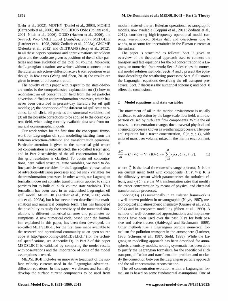
Table 1. Oil spill model state variables. Four are structural state variables or concentrations, eight are oil slick state variables used for thetransformation processes, four are particle state variables used to solve for the advection–diffusion processes.

Variable Variable type Variable name Dimensions

CS(x,y, t) Structural Oil concentration at the surface kg m−2

CD(x,y, t) Structural Oil concentration dispersed kg m−2

CC(x,y, t) Structural Oil concentration on the coast kg m−1

CB(x,y, t) Structural Oil concentration at the bottom kg m−2

VS(x,y, t) Slick Oil slick surface volume m3

VD(x,y, t) Slick Oil slick subsurface (dispersed) volume m3

V TK(x,y, t) Slick Thick part of the surface oil slick volume m3

V TN(x,y, t) Slick Thin part of the surface oil slick volume m3

ATK(t) Slick Surface area of the thick part of the surface oil slick volume m2

ATN(t) Slick Surface area of the thin part of the surface oil slick volume m2

T TK(x,y, t) Slick Surface thickness of the thick part of the surface oil slick volume m

T TN(x,y, t) Slick Surface thickness of the thin part of the surface oil slick volume m

xk(t) = (xk(t),yk(t),zk(t)) Particle Particle position m

υNE(nk, t) Particle Non-evaporative surface oil volume particle attribute m3

υE(nk, t) Particle Evaporative surface oil volume particle attribute m3

σ(nk, t) = 0,1,2,< 0 Particle Particle status index (on surface, dispersed, sedimented, on coast) –

the most important of these is the consideration that the con-stituent particles do not influence water hydrodynamics andprocesses. This assumption has limitations at the surface ofthe ocean because floating oil locally modifies air–sea inter-actions and surface wind drag. Furthermore, the constituentparticles move through infinitesimal displacements withoutinertia (like water parcels) and without interacting amongstthemselves. After such infinitesimal displacements, the vol-ume associated with each particle is modified due to thephysical and chemical processes acting on the entire slickrather than on the single particles properties. This is a fun-damental assumption that differentiates oil slick Lagrangianmodels from marine biochemical tracer Lagrangian models,where single particles undergo biochemical transformations(Woods, 2002).

If we apply these assumptions to Eq. (1), we effectivelysplit the active tracer equation into two component equations:

∂C1

∂t=

M∑j=1

rj (x,C1(x, t), t) (2)

and

∂C

∂t= −U · ∇C1 + ∇ · (K∇C1), (3)

whereC1 is the oil concentration solution solely due to theweathering processes, while the final time rate of change ofC

is given by the advection–diffusion acting onC1. The modelsolves Eq. (2) by considering the transformation processesacting on the total oil slick volume, and oil slick state vari-ables are defined. The Lagrangian particle formalism is thenapplied to solve Eq. (3), discretizing the oil slick in parti-cles with associated particle state variables, some of themdeduced from the oil slick state variables. The oil concentra-tion is then computed by assembling the particles togetherwith their associated properties. While solving Eq. (3) withLagrangian particles is well known (Griffa, 1996), the con-nection between Eqs. (2) and (3), explained in this paper, iscompletely new.

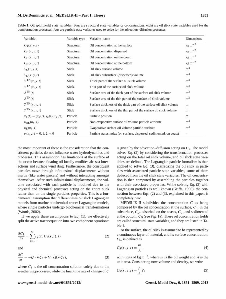
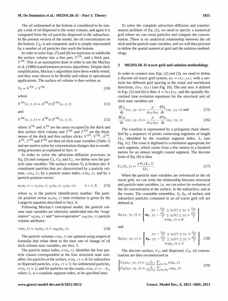
MEDSLIK-II subdivides the concentrationC as beingcomposed by the oil concentration at the surface,CS, in thesubsurface,CD, adsorbed on the coasts,CC, and sedimentedat the bottom,CB (see Fig.1a). These oil concentration fieldsare called structural state variables, and they are listed in Ta-ble1.

At the surface, the oil slick is assumed to be represented bya continuous layer of material, and its surface concentration,CS, is defined as

CS(x,y, t) =m

A, (4)

with units of kg m−2, wherem is the oil weight andA is theunit area. Considering now volume and density, we write

CS(x,y, t) =ρ

AVS. (5)

www.geosci-model-dev.net/6/1851/2013/ Geosci. Model Dev., 6, 1851–1869, 2013


x

y

z

A)

- HB Bottom

CB

CD

CC

CS

x

y

z

B)

- HB Bottom

xT

yT

zT

δxT

δyT σ=0

σ=1

- HB Bottom

σ=2

LC

x

y

z

D)

- HB Bottom

(xk, yk, zk)

xT

yT

δxT

C)

σ= -Li

δLi

Fig. 1. Schematic view of the oil tracer grids (the grey spheres represent the oil particles):(a) graphical representation of concentrationclasses;(b) 3-D view of one cell of the oil tracer grid for weathering processes:σ is the particle status index andHB indicates the bottomdepth of theδxT ,δyT cell ; (c) 2-D view of the oil tracer grid for weathering processes and coastline polygonal chain (red); and(d) 3-D viewof the oil tracer grid for advection–diffusion processes.

In the subsurface, oil is formed by droplets of various sizesthat can coalesce again with the surface oil slick or sedimentat the bottom. The subsurface or dispersed oil concentration,CD, can then be written for all droplets composing the dis-persed oil volumeVD as

CD(x,y, t) =ρ

AVD. (6)

The weathering processes in Eq. (2) are now applied toCSandCD and in particular to oil volumes:

dCS

dt=

ρ

A

dVS

dtand (7)

dCD

dt=

ρ

A

dVD

dt. (8)

The surface and dispersed oil volumes,VS andVD, are thebasic oil slick state variables of our problem (see Table1).Equations (7) and (8) are the MEDSLIK-II equations for theconcentrationC1 in Eq. (2), being split simply intoVS andVDthat are changed by weathering processes calculated usingtheMackay et al.(1980) fate algorithms that will be reviewedin Sect.4.

When the surface oil arrives close to the coasts, defined bya reference segmentLC, it can be adsorbed and the concen-tration of oil at the coasts,CC, is defined as

CC(x,y, t) =ρ

LCVC, (9)

whereVC is the adsorbed oil volume. The latter is calculatedfrom the oil particle state variables, to be described below,and there is no prognostic equation explicitly written forVC.



The oil sedimented at the bottom is considered to be sim-ply a sink of oil dispersed in the water column, and again it iscomputed from the oil particles dispersed in the subsurface.In the present version of the model, the oil concentration onthe bottom,CB, is not computed, and it is simply representedby a number of oil particles that reach the bottom.

In order to solve Eqs. (7) and (8) we need now to subdividethe surface volume into a thin part,V TN, and a thick part,V TK . This is an assumption done in order to use theMackayet al.(1980) transformation process algorithms. Despite theirsimplification, Mackay’s algorithms have been widely tested,and they were shown to be flexible and robust in operationalapplications. The surface oil volume is then written as

VS = V TN+ V TK, (10)

where

V TN(x,y, t) = ATN(t)T TN(x,y, t) (11)

and

V TK(x,y, t) = ATK(t)T TK(x,y, t). (12)

whereATK andATN are the areas occupied by the thick andthin surface slick volume andT TK andT TN are the thick-nesses of the thick and thin surface slicks.V TN, V TK , ATN,ATK , T TN andT TK are then oil slick state variables (Table1)and are used to solve for concentration changes due to weath-ering processes as explained in Sect.4.

In order to solve the advection–diffusion processes inEq. (3) and computeCS, CD andCC, we define now the par-ticle state variables. The surface volumeVS is broken intoNconstituent particles that are characterized by a particle vol-ume,υ(nk, t), by a particle status index,σ(nk, t), and by aparticle position vector:

xk(nk, t) = (xk(nk, t),yk(nk, t),zk(nk, t)), k = 1,N, (13)

where nk is the particle identification number. The parti-cle position vectorxk(nk, t) time evolution is given by theLangevin equation described in Sect.6.

Following Mackay’s conceptual model, the particle vol-ume state variables are ulteriorly subdivided into the “evap-orative” υE(nk, t) and “non-evaporative”υNE(nk, t) particlevolume attributes:

υ(nk, t) = υE(nk, t) + υNE(nk, t). (14)

The particle volumesυ(nk, t) are updated using empiricalformulas that relate them to the time rate of change of oilslick volume state variables, see Sect.5.

The particle status index,σ(nk, t), identifies the four par-ticle classes correspondent to the four structural state vari-ables: for particles at the surface,σ(nk, t) = 0; for subsurfaceor dispersed particles,σ(nk, t) = 1; for sedimented particles,σ(nk, t) = 2; and for particles on the coasts,σ(nk, t) = −Li ,whereLi is a coastline segment index, to be specified later.

To solve the complete advection–diffusion and transfor-mation problem of Eq. (1), we need to specify a numericalgrid where we can count particles and compute the concen-tration. There is no analytical relationship between the oilslick and the particle state variables, and we will then proceedto define the spatial numerical grid and the solution method-ology.

3 MEDSLIK-II tracer grid and solution methodology

In order to connect now Eqs. (2) and (3), we need to definea discrete oil tracer grid system,xT = (xT ,yT ), with a uni-form but different grid spacing in the zonal and meridionaldirections,(δxT ,δyT ) (see Fig.1b). The unit areaA definedin Eqs. (5) and (6) is thenA = δxT δyT , and the spatially dis-cretized time evolution equations for the structural and oilslick state variables are

dCS

dt(xT ,yT , t) =

ρ

δxT δyT

dVS

dt(xT ,yT , t) and (15)

dCD

dt(xT ,yT , t) =

ρ

δxT δyT

dVD

dt(xT ,yT , t) (16)

The coastline is represented by a polygonal chain identi-fied by a sequence of points connecting segments of lengthδLi , identified by the coastline segment index,Li (seeFig. 1c). The coast is digitised to a resolution appropriate foreach segment, which varies from a few metres to a hundredmetres for an almost straight coastal segment. The discreteform of Eq. (9) is then

CC(Li, t) =ρVC(Li, t)

δLi. (17)

When the particle state variables are referenced to the oiltracer grid, we can write the relationship between structuraland particle state variables, i.e. we can solve for evolution ofthe oil concentration at the surface, in the subsurface, and atthe coasts. The countable ensembles,IS,ID, of surface andsubsurface particles contained in an oil tracer grid cell aredefined as

IS(xT ,yT , t) =

nk;

xT −δxT

2 ≤ xk(t) ≤ xT +δxT

2yT −

δyT

2 ≤ yk(t) ≤ yT +δyT

2σ(nk, t) = 0

and

ID(xT ,yT , t) =

nk;

xT −δxT

2 ≤ xk(t) ≤ xT +δxT

2yT −

δyT

2 ≤ yk(t) ≤ yT +δyT

2σ(nk, t) = 1

. (18)

The discrete surface,CS, and dispersed,CD, oil concen-trations are then reconstructed as{

CS(xT ,yT , t) =ρ

δxT δyT

∑nkεIS

υ(nk, t)

CD(xT ,yT , t) =ρ

δxT δyT

∑nkεID

υ(nk, t).(19)



The oil concentration for particles on the coasts,CC(Li, t),is calculated usingIC(Li, t), which is the set of particles“beached” on the coastal segmentLi :

IC(Li, t) = {nk;σ(nk, t) = −Li}. (20)

The concentration of oil on each coastal segment is calcu-lated by

CC(Li, t) =ρ

δLi

∑nkεIC

υ(nk, t). (21)

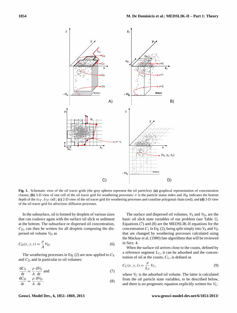
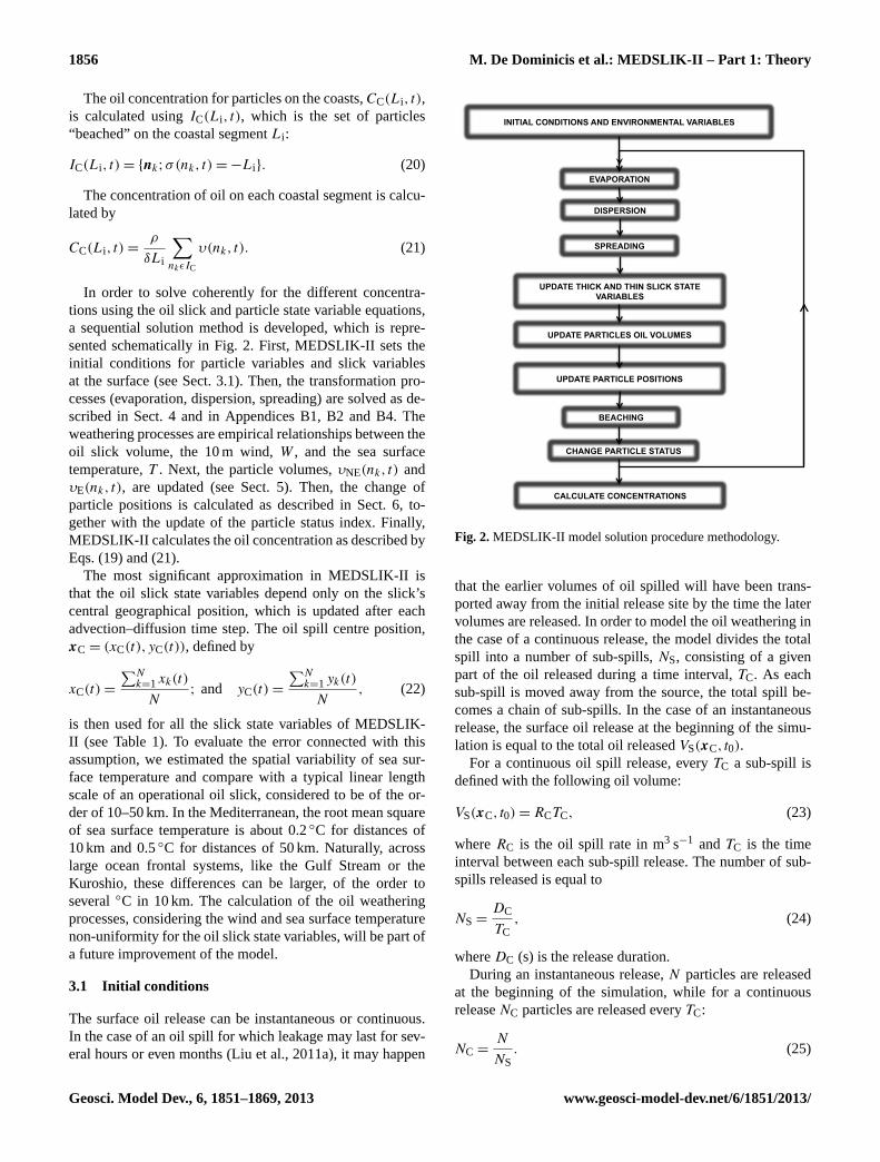
In order to solve coherently for the different concentra-tions using the oil slick and particle state variable equations,a sequential solution method is developed, which is repre-sented schematically in Fig.2. First, MEDSLIK-II sets theinitial conditions for particle variables and slick variablesat the surface (see Sect.3.1). Then, the transformation pro-cesses (evaporation, dispersion, spreading) are solved as de-scribed in Sect.4 and in AppendicesB1, B2 and B4. Theweathering processes are empirical relationships between theoil slick volume, the 10 m wind,W , and the sea surfacetemperature,T . Next, the particle volumes,υNE(nk, t) andυE(nk, t), are updated (see Sect.5). Then, the change ofparticle positions is calculated as described in Sect.6, to-gether with the update of the particle status index. Finally,MEDSLIK-II calculates the oil concentration as described byEqs. (19) and (21).

The most significant approximation in MEDSLIK-II isthat the oil slick state variables depend only on the slick’scentral geographical position, which is updated after eachadvection–diffusion time step. The oil spill centre position,xC = (xC(t),yC(t)), defined by

xC(t) =

∑Nk=1xk(t)

N; and yC(t) =

∑Nk=1yk(t)

N, (22)

is then used for all the slick state variables of MEDSLIK-II (see Table1). To evaluate the error connected with thisassumption, we estimated the spatial variability of sea sur-face temperature and compare with a typical linear lengthscale of an operational oil slick, considered to be of the or-der of 10–50 km. In the Mediterranean, the root mean squareof sea surface temperature is about 0.2◦C for distances of10 km and 0.5◦C for distances of 50 km. Naturally, acrosslarge ocean frontal systems, like the Gulf Stream or theKuroshio, these differences can be larger, of the order toseveral◦C in 10 km. The calculation of the oil weatheringprocesses, considering the wind and sea surface temperaturenon-uniformity for the oil slick state variables, will be part ofa future improvement of the model.

3.1 Initial conditions

The surface oil release can be instantaneous or continuous.In the case of an oil spill for which leakage may last for sev-eral hours or even months (Liu et al., 2011a), it may happen

INITIAL CONDITIONS AND ENVIRONMENTAL VARIABLES

EVAPORATION

DISPERSION

SPREADING

UPDATE PARTICLES OIL VOLUMES

UPDATE PARTICLE POSITIONS

CALCULATE CONCENTRATIONS

UPDATE THICK AND THIN SLICK STATE VARIABLES

BEACHING

CHANGE PARTICLE STATUS

Fig. 2.MEDSLIK-II model solution procedure methodology.

that the earlier volumes of oil spilled will have been trans-ported away from the initial release site by the time the latervolumes are released. In order to model the oil weathering inthe case of a continuous release, the model divides the totalspill into a number of sub-spills,NS, consisting of a givenpart of the oil released during a time interval,TC. As eachsub-spill is moved away from the source, the total spill be-comes a chain of sub-spills. In the case of an instantaneousrelease, the surface oil release at the beginning of the simu-lation is equal to the total oil releasedVS(xC, t0).

For a continuous oil spill release, everyTC a sub-spill isdefined with the following oil volume:

VS(xC, t0) = RCTC, (23)

whereRC is the oil spill rate in m3 s−1 andTC is the timeinterval between each sub-spill release. The number of sub-spills released is equal to

NS =DC

TC, (24)

whereDC (s) is the release duration.During an instantaneous release,N particles are released

at the beginning of the simulation, while for a continuousreleaseNC particles are released everyTC:

NC =N

NS. (25)



Each initial particle volume,υ(nk, t0), is defined as

υ(nk, t0) =NSVS(xC, t0)

N, (26)

where in the case of an instantaneous releaseNS is equal to 1.The initial evaporative and non-evaporative oil volume

components, for both instantaneous and continuous release,are defined as

υE(nk, t0) = (1−ϕNE

100)υ(nk, t0) and (27)

υNE(nk, t0) =ϕNE

100υ(nk, t0), (28)

whereϕNE is the percentage of the non-evaporative compo-nent of the oil that depends on the oil type. The initializationof the thin and thick area values is taken from the initial sur-face amount of oil released using the relative thicknesses andF , which is the area ratio of the two slick parts,ATK andATN. Using Eqs. (10), (11) and (12), we therefore write

ATN(t0) = FATK(t0) and (29)

ATK(t0) =VS(xC, t0)

T TK(xC, t0) + FT TN(xC, t0). (30)

The same formula is valid for both instantaneous or con-tinuous release. The initial valuesT TK(xC, t0), T TN(xC, t0)

andF have to be defined as input.F can be in a range be-tween 1 and 1000, standardT TK(xC, t0) are between 1×10−4

−0.02 m, whileT TN(xC, t0) lies between 1×10−6 and1×10−5 m (standard values are summarized in Table2). Fora pointwise oil spill source higher values ofT TK(xC, t0) andT TN(xC, t0) and lower values ofF are recommended. Forinitially extended oil slicks at the surface (i.e. slicks observedby satellite or aircraft), lower thicknesses and higher valuesof F can be used. In the latter case, the initial slick area,A = ATN

+ ATK , can be provided by satellite images and thethicknesses extracted from other information.

4 Time rate of change of slick state variables

Using Eq. (10), the time rate of change of oil volume is writ-ten as

∂VS

∂t=

∂V TK

∂t+

∂V TN

∂t. (31)

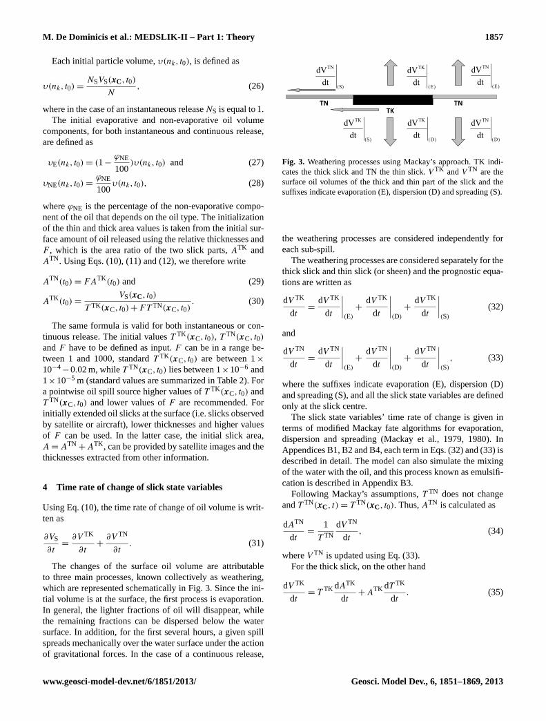
The changes of the surface oil volume are attributableto three main processes, known collectively as weathering,which are represented schematically in Fig.3. Since the ini-tial volume is at the surface, the first process is evaporation.In general, the lighter fractions of oil will disappear, whilethe remaining fractions can be dispersed below the watersurface. In addition, for the first several hours, a given spillspreads mechanically over the water surface under the actionof gravitational forces. In the case of a continuous release,

TK TN TN

Fig. 3. Weathering processes using Mackay’s approach. TK indi-cates the thick slick and TN the thin slick.V TK andV TN are thesurface oil volumes of the thick and thin part of the slick and thesuffixes indicate evaporation (E), dispersion (D) and spreading (S).

the weathering processes are considered independently foreach sub-spill.

The weathering processes are considered separately for thethick slick and thin slick (or sheen) and the prognostic equa-tions are written as

dV TK

dt=

dV TK

dt

∣∣∣∣(E)

+dV TK

dt

∣∣∣∣(D)

+dV TK

dt

∣∣∣∣(S)

(32)

and

dV TN

dt=

dV TN

dt

∣∣∣∣(E)

+dV TN

dt

∣∣∣∣(D)

+dV TN

dt

∣∣∣∣(S)

, (33)

where the suffixes indicate evaporation (E), dispersion (D)and spreading (S), and all the slick state variables are definedonly at the slick centre.

The slick state variables’ time rate of change is given interms of modified Mackay fate algorithms for evaporation,dispersion and spreading (Mackay et al., 1979, 1980). InAppendicesB1, B2 andB4, each term in Eqs. (32) and (33) isdescribed in detail. The model can also simulate the mixingof the water with the oil, and this process known as emulsifi-cation is described in AppendixB3.

Following Mackay’s assumptions,T TN does not changeandT TN(xC, t) = T TN(xC, t0). Thus,ATN is calculated as

dATN

dt=

1

T TN

dV TN

dt, (34)

whereV TN is updated using Eq. (33).For the thick slick, on the other hand

dV TK

dt= T TK dATK

dt+ ATK dT TK

dt. (35)



The area of the thick slick,ATK , only changes due tospreading, thus

dATK

dt=

dATK

dt

∣∣∣∣(S)

, (36)

where the time rate of change of the thick area due to spread-ing is given by Eq. (B20). V TK is updated using Eq. (32) andthe thickness changes are calculated diagnostically by

T TK=

V TK

ATK . (37)

5 Time rate of change of particle oil volumestate variables

The particle oil volumes, defined by Eq. (14), are changedafter the transformation processes have acted on the oil slickvariables. For all particle status indexσ(nk, t), the evapora-tive oil particle volume changes following the empirical re-lationship

υE(nk, t) =

[(1−

ϕNE

100

)− f (E)(xC, t)

]υ(nk, t0), (38)

wheref (E) is the fraction of oil evaporated defined as

f (E)(xC, t) =

V TK(xC, t)∣∣(E)

+ V TN(xC, t)∣∣(E)

V TK(t0) + V TN(t0)(39)

and V TK(xC, t)∣∣(E)

and V TN(xC, t)∣∣(E)

are the volumes ofoil evaporated from the thick and thin slicks, respectively,calculated using Eqs. (B1) and (B5).

For both “surface” and “dispersed” particles (σ(nk, t) = 0and σ(nk, t) = 1), the non-evaporative oil component,υNE(nk, t), does not change, while a certain fraction of thenon-evaporative oil component of a beached particle can bemodified due to adsorption processes occurring on a partic-ular coastal segment, seeping into the sand or forming a tarlayer on a rocky shore. For the “beached” particles, the par-ticle non-evaporative oil component is then reduced to

υNE(nk, t) = υNE(nk, t∗

0 )0.5t−t∗0

TS(Li ) , σ (nk, t) = −i, (40)

wheret∗0 is the instant at which the particle passes from sur-face to beached status and vice versa,TS(Li) is a half-lifefor seepage or any other mode of permanent attachment tothe coasts. Half-life is a parameter which describes the “ab-sorbency” of the shoreline by describing the rate of entrain-ment of oil after it has landed at a given shoreline (Shen et al.,1987). The half-life depends on the coastal type, for examplesand beach or rocky coastline. Example values are given inTable2.

6 Time rate of change of particle positions

The time rate of change of particle positions in the oil tracergrid is given bynk uncoupled Langevin equations:

dxk(t)

dt= A(xk, t) + B(xk, t)ξ(t), (41)

where the tensorA(xk, t) represents what is known as the de-terministic part of the flow field, corresponding to the meanfield U in Eq. (1), while the second term is a stochastic term,representing the diffusion term in Eq. (1). The stochastic termis composed of the tensorB(xk, t), which characterizes ran-dom motion, andξ(t), which is a random factor. If we de-fine the Wiener processW(t) =

∫ t

0 ξ(s)ds and apply the Itoassumption (Tompson and Gelhar, 1990), Eq. (41) becomesequivalent to the Ito stochastic differential equation:

dxk(t) =A(xk, t)dt + B(xk, t)dW (t), (42)

where dt is the Lagrangian time step and dW (t) is a randomincrement. The Wiener process describes the path of a par-ticle due to Brownian motion modelled by independent ran-dom increments dW (t) sampled from a normal distributionwith zero mean,〈dW(t)〉 = 0 and second order moment with〈dW · dW 〉 = dt . Thus, we can replace dW (t) in Eq. (42)with a vectorZ of independent random numbers, normallydistributed, i.e.Z ∈ N(0,1), and multiplied by

√dt :

dxk(t) =A(xk, t)dt + B(xk, t)Z√

dt . (43)

The unknown tensorsA(xk, t) andB(xk, t) in Eq. (43) aremost commonly written as (Risken, 1989):

dxk(t) = (44)

=

U(xk, t)

V (xk, t)

W(xk, t)

dt +

√2Kx 0 00

√2Ky 0

0 0√

2Kz

Z1Z2Z3

√dt,

whereA was assumed to be diagonal and equal to the Eule-rian field velocity components,B is again diagonal and equalto Kx,Ky,Kz turbulent diffusivity coefficients in the threedirections, andZ1,Z2,Z3 are random vector amplitudes. Forparticles at the surface and dispersed, Eq. (45) takes the fol-lowing form:

dxk(t) =

U(xk,yk,zk, t)

V (xk,yk,zk, t)

0

dt +

dx′

k(t)

dy′

k(t)

dz′

k(t)

, (45)

where for simplicity we have indicated with dx′

k(t), dy′

k(t),dz′

k(t) the turbulent transport terms written in Eq. (45). Forparticles at the surface, the vertical position does not change:zk = 0 and dz′

k(t) = 0. Thezk can only change when the par-ticles become dispersed and the horizontal velocity at the ver-tical position of the particle is used to displace the dispersedparticles.



The deterministic transport terms in Eq. (45) are now ex-panded in different components:

σ = 0 dxk(t) =[UC(xk,yk,0, t) + UW(xk,yk, t)

+US(xk,yk, t)]dt + dx′

k(t)

σ = 1 dxk(t) = UC(xk,yk,zk, t)dt + dx′

k(t)

, (46)

whereUC, is the Eulerian current velocity term due to a com-bination of non-local wind and buoyancy forcings, mainlycoming from operational oceanographic numerical modelforecasts or analyses;UW, called hereafter the local wind ve-locity term, is a velocity correction term due mainly to errorsin simulating the wind-driven mean surface currents (Ekmancurrents); andUS, called hereafter the wave current term, isthe velocity due to wave-induced currents or Stokes drift. Inthe following two subsections we will describe the differentvelocity components introduced in Eq. (46).

6.1 Current and local wind velocity terms

Ocean currents near the ocean surface are attributable tothe effects of atmospheric forcing, which can be subdividedinto two main categories, buoyancy fluxes and wind stresses.Wind stress forcing is by far the more important in termsof kinetic energy of the induced motion, accounting for70 % or more of current amplitude over the oceans (Wun-sch, 1998). One part of wind-induced currents is attributableto non-local winds, and is dominated by geostrophic orquasi-geostrophic dynamic balances (Pedlosky, 1986). Bydefinition, geostrophic and quasi-geostrophic motion hasa timescale of several days and characterizes oceanicmesoscale motion, a very important component of the large-scale flow field included inU . It is customary to indicate thatgeostrophic or quasi-geostrophic currents dominate belowthe mixed layer, even though they can sometimes emerge andbe dominant in the upper layer. The mixed layer dynamicsare typically considered to be ageostrophic, and the dominanttime-dependent, wind-induced currents in the surface layerare the Ekman currents due to local winds (Price et al., 1987;Lenn and Chereskin, 2009). All these components should beadequately considered in theUC field of Eq. (46). In thepast, oil spill modellers computedUC(xk, t) from clima-tological data using the geostrophic assumption (Al-Rabehet al., 2000). The ageostrophic Ekman current componentswere thus added by the termUW(xk, t). It is well knownthat Ekman currents at the surfaceUW = (UW,VW) can beparameterized as a function of wind intensity and angle be-tween winds and currents, i.e.

UW = α(Wx cosβ + Wy sinβ

)and

VW = α(−Wx sinβ + Wy cosβ

)(47)

whereWx andWy are the wind zonal and meridional compo-nents at 10 m, respectively, andα andβ are two parametersreferred to as drift factor and drift angle. There has been con-siderable dispute among modellers on the choice of the best

values of the drift factor and angle, with most models usinga value of around 3 % for the former and between 0◦and 25◦

for the latter (Al-Rabeh et al., 2000).With the advent of operational oceanography and accu-

rate operational models of circulation (Pinardi and Coppini,2010; Pinardi et al., 2003; Zodiatis et al., 2008b), currentvelocity fields can be provided by analyses and forecasts,available hourly or daily, produced by high-resolution oceangeneral circulation models (OGCMs). The wind drift termas reported in Eq. (47) may be optional when using surfacecurrents coming from an oceanographic model that resolvesthe upper ocean layer dynamics, as also found byLiu etal. (2011b) andHuntley et al.(2011). In such cases, addingUW(xk, t) could worsen the results, as shown in Fig. 2 ofPart 2. When the wind drift term is used with a 0◦ deviationangle, this term should not be considered as an Ekman cur-rent correction, but a term that could account for other near-surface processes that drive the movement of the oil slick, asshown in one case study of Part 2 (Fig. 4). This theme willbe revisited in Part 2 of this paper, where the sensitivity ofLagrangian trajectories to the different corrections applied tothe ocean current field will be assessed.

6.2 Wave current term

Waves give rise to transport of pollutants by wave-inducedvelocities that are known as Stokes drift velocity,US(xk, t)

(see AppendixC). This current component should certainlybe added to the current velocity field from OGCMs (Sobeyand Barker, 1997; Pugliese Carratelli et al., 2011; Röhrs etal., 2012), as normally most ocean models are not coupledwith wave models. Stokes drift is the net displacement of aparticle in a fluid due to wave motion, resulting essentiallyfrom the fact that the particle moves faster forward when theparticle is at the top of the wave circular orbit than it doesbackward when it is at the bottom of its orbit. Stokes drifthas been introduced into MEDSLIK-II using an analyticalformulation that depends on wind amplitude. In the future,Stokes drift should come from complex wave models, run inparallel with MEDSLIK-II.

Considering the surface, the Stokes drift velocity intensityin the direction of the wave propagation is (see AppendixC)

DS(z = 0) = 2

∞∫0

ωk(ω)S(ω)dω, (48)

whereω is angular frequency,k is wave-number, andS(ω) iswave spectrum.

Equation (48) has been implemented in MEDSLIK-II byconsidering the direction of wave propagation to be equalto the wind direction. The Stokes drift velocity components,US, are

US = DScosϑ andVS = DSsinϑ , (49)



whereϑ = arctg(

Wx

Wy

)is the wind direction, andWx andWy

are the 10 m height wind zonal and meridional components.

6.3 Turbulent diffusivity terms

It is preferable to parameterize the normally distributed ran-dom vectorZ in Eq. (42) with a random number generatoruniformly distributed between 0 and 1. We assume that theparticle moving through the fluid receives a random impulseat each time step, due to the action of incoherent turbulentmotions, and that it has no memory of its previous turbulentdisplacement. This can be written as

dx′

k(t) = (2r − 1)d , (50)

whered is the particle mean path andr is a random realnumber taking values between 0 and 1 with a uniform dis-tribution. The mean square displacement of Eq. (50) is⟨dxk

′(t)2⟩=∫ 1

0 [(2r − 1)d]2dr =13d2, (51)

while the mean square displacement of the turbulent termsin Eq. (45) is simply dx′

k(t)2= 2Kdt . Equating the mean

square displacements, we have

d2= 6Kxdt

d2= 6Kydt

d2= 6Kzdt .

(52)

Finally, the stochastic transport terms in MEDSLIK-II arethen written as

dx′

k(t) = Z1√

2Kxdt = [2r − 1]√

6Khdt

dy′

k(t) = Z2√

2Kydt = [2r − 1]√

6Khdt

dz′

k(t) = Z3√

2Kzdt = [2r − 1]√

6Kvdt,

, (53)

whereKh andKv are prescribed turbulent horizontal and ver-tical diffusivities. As for modern high resolution Eulerianmodels, horizontal diffusivity is considered to be isotropicand the values used are in the range 1–100 m2 s−1, consistentwith the estimation of Lagrangian diffusivity carried out byDe Dominicis et al.(2012) and indicated byASCE (1996).Regarding the vertical diffusion, the vertical diffusivity in themixed layer, assumed to be 30 m deep, is set to 0.01 m2 s−1,while below it is 0.0001 m2 s−1 (see Table2). This values isintermediate between the molecular viscosity value for wa-ter, i.e. 10−6 m2 s−1, usually reached below 1000 m, and themixed layer values.

7 Numerical considerations

Numerical considerations for MEDSLIK-II are connected tothe interpolation method between input fields and the oiltracer grid, to the numerical scheme used to solve Eqs. (32),(33) and (45), to the model time step and to the oil tracer gridselection.

7.1 Interpolation method

The environmental variables of interest are the atmosphericwind, the ocean currents and the sea surface temperature.They are normally supplied on a different numerical grid thanthe oil slick centre or particle locations. For the advectioncalculation, interpolation is thus required to compute the cur-rents and winds at the particle locations. While for the trans-formation processes calculation, sea surface temperature andwinds are interpolated at the slick centre.

Let us indicate with (xE,yE,zE) the numerical gridon which the environmental variables, collectively indi-cated by q, are provided by the Eulerian meteorologi-cal/oceanographic models.

First, a preprocessing procedure is needed to reconstructthe currents in the zone between the last water grid node ofthe oceanographic model and the real coastline. MEDSLIK-II employs a procedure to “extrapolate” the currents overland points and thus to add a velocity field value on land.If (xE(i),yE(i)) is considered to be a land grid node by themodel, the current velocities component,qxE(i), yE(i), at thecoastal grid point(xE(i), yE(i)), is set equal to the averageof the nearby values, when there are at least two neighbour-ing points(NWP >= 2); that means

qxE(i),yE(i) =

qxE(i+1),yE(i)+qxE(i−1),yE(i)+qxE(i),yE(i−1)+qxE(i),yE(i+1)

NWP.

(54)

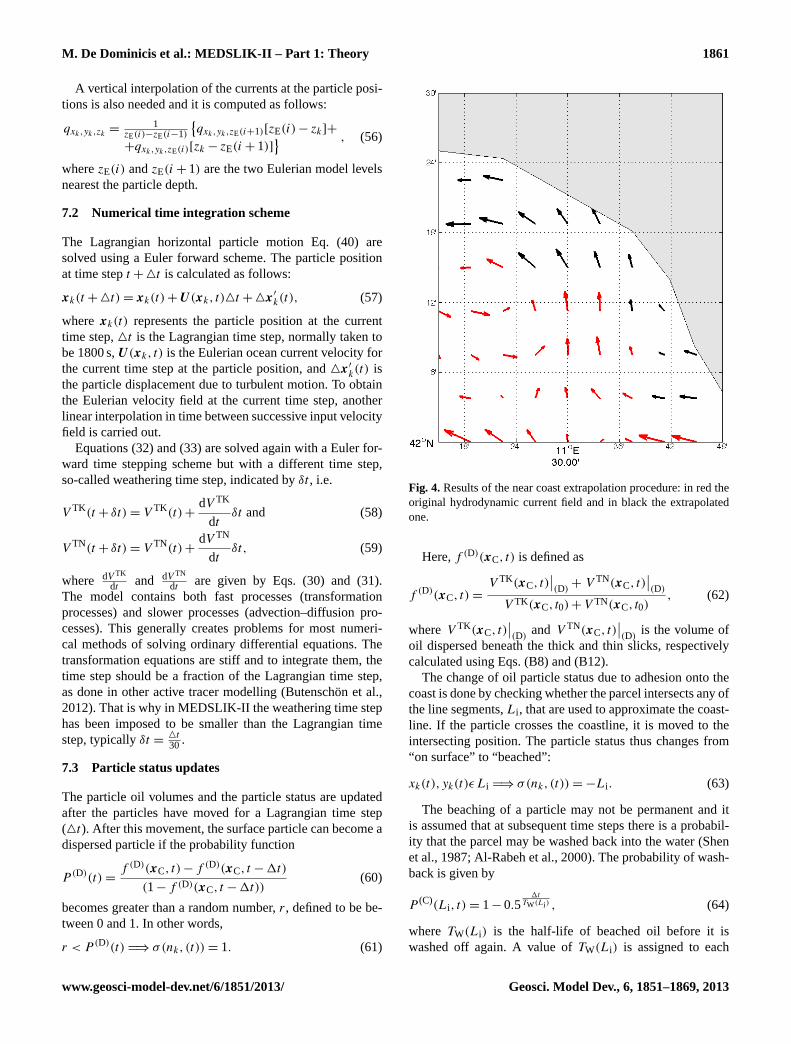
The result of this extrapolation is shown in Fig.4. If thecurrent velocities components are given on a staggered grid, afurther initial interpolation is also needed to bring both com-ponents on the same grid point before the extrapolation isdone.

Then, the winds and currents are computed at the parti-cle position(xk,yk), for a fixed depthzE, with the followinginterpolation algorithm:

q1 = qxE(i),yE(i)[xE(i + 1) − xk]

q2 = qxE(i+1),yE(i)[xk − xT (i)]

q3 = qxE(i),yE(i+1)[xE(i + 1) − xk]

q4 = qxE(i+1),yE(i+1)[xk − xE(i)]

qxk,yk=

(q1+ q2)[yE(i + 1) − yk] + (q3+ q4)[yk − yE(i)]

1xE1yE. (55)

where (xk,yk) is the particle position referenced to theoil tracer grid, (xE(i),yE(i)), (xE(i + 1),yE(i)), (xE(i +

1),yE(i+1)), and(xE(i),yE(i+1)) are the four external fieldgrid points nearest the particle position and1xE,1yE arethe horizontal grid spacings of the Eulerian model (oceano-graphic or meteorological). Using the same algorithm, thewind and sea surface temperature are interpolated to the oilslick centre,(xC(t),yC(t)), defined by Eq. (22).



A vertical interpolation of the currents at the particle posi-tions is also needed and it is computed as follows:

qxk,yk,zk=

1zE(i)−zE(i−1)

{qxk,yk,zE(i+1)[zE(i) − zk]+

+qxk,yk,zE(i)[zk − zE(i + 1)]} , (56)

wherezE(i) andzE(i + 1) are the two Eulerian model levelsnearest the particle depth.

7.2 Numerical time integration scheme

The Lagrangian horizontal particle motion Eq. (40) aresolved using a Euler forward scheme. The particle positionat time stept + 4t is calculated as follows:

xk(t + 4t) = xk(t) + U(xk, t)4t + 4x′

k(t), (57)

wherexk(t) represents the particle position at the currenttime step,4t is the Lagrangian time step, normally taken tobe 1800 s,U(xk, t) is the Eulerian ocean current velocity forthe current time step at the particle position, and4x′

k(t) isthe particle displacement due to turbulent motion. To obtainthe Eulerian velocity field at the current time step, anotherlinear interpolation in time between successive input velocityfield is carried out.

Equations (32) and (33) are solved again with a Euler for-ward time stepping scheme but with a different time step,so-called weathering time step, indicated byδt , i.e.

V TK(t + δt) = V TK(t) +dV TK

dtδt and (58)

V TN(t + δt) = V TN(t) +dV TN

dtδt, (59)

where dV TK

dtand dV TN

dtare given by Eqs. (30) and (31).

The model contains both fast processes (transformationprocesses) and slower processes (advection–diffusion pro-cesses). This generally creates problems for most numeri-cal methods of solving ordinary differential equations. Thetransformation equations are stiff and to integrate them, thetime step should be a fraction of the Lagrangian time step,as done in other active tracer modelling (Butenschön et al.,2012). That is why in MEDSLIK-II the weathering time stephas been imposed to be smaller than the Lagrangian timestep, typicallyδt =

4t30 .

7.3 Particle status updates

The particle oil volumes and the particle status are updatedafter the particles have moved for a Lagrangian time step(4t). After this movement, the surface particle can become adispersed particle if the probability function

P (D)(t) =f (D)(xC, t) − f (D)(xC, t − 1t)

(1− f (D)(xC, t − 1t))(60)

becomes greater than a random number,r, defined to be be-tween 0 and 1. In other words,

r < P (D)(t) H⇒ σ(nk, (t)) = 1. (61)

Fig. 4. Results of the near coast extrapolation procedure: in red theoriginal hydrodynamic current field and in black the extrapolatedone.

Here,f (D)(xC, t) is defined as

f (D)(xC, t) =

V TK(xC, t)∣∣(D)

+ V TN(xC, t)∣∣(D)

V TK(xC, t0) + V TN(xC, t0), (62)

where V TK(xC, t)∣∣(D)

and V TN(xC, t)∣∣(D)

is the volume ofoil dispersed beneath the thick and thin slicks, respectivelycalculated using Eqs. (B8) and (B12).

The change of oil particle status due to adhesion onto thecoast is done by checking whether the parcel intersects any ofthe line segments,Li , that are used to approximate the coast-line. If the particle crosses the coastline, it is moved to theintersecting position. The particle status thus changes from“on surface” to “beached”:

xk(t),yk(t)ε Li H⇒ σ(nk, (t)) = −Li . (63)

The beaching of a particle may not be permanent and itis assumed that at subsequent time steps there is a probabil-ity that the parcel may be washed back into the water (Shenet al., 1987; Al-Rabeh et al., 2000). The probability of wash-back is given by

P (C)(Li, t) = 1− 0.51t

TW(Li ) , (64)

where TW(Li) is the half-life of beached oil before it iswashed off again. A value ofTW(Li) is assigned to each



coastal segment depending on the coastal type. Examplevalues are given in Table2. At each time step, for each“beached” particle a random number generator,r, is calledup and the parcel is released back into the water (its statusreturns to “surface”) if

r < P (C)(t) H⇒ σ(nk, (t)) = 0. (65)

When a particle is washed back, it is of course depleted bythe oil that has become permanently attached (Eq.40) andits new position is calculated using Eq. (46). The model doesnot follow any further the oil fraction that is permanently de-posited on the coast. It is important to realize that whole par-ticles are not lost as permanently beached, but only a fractionof them. The actual number of particles remains constant.

The deposition of a particle on the bottom is the onlycase in which a particle is lost from the model. However,no proper parameterization of sedimentation is now includedinto the model. The particles are considered to be lost fromthe water column when they are less than 20 cm from thebottom. Thus, the particle status changes from “dispersed”to “sedimented” can be written as

HB(xk,yk) − zk < 20 cmH⇒ σ(nk, (t)) = 2, (66)

whereHB(xk,yk) is the bottom depth below the particle po-sition.

7.4 Oil tracer grid and number of particles

The oil tracer grid resolution,δxT , and the total number ofparticles,N , used to discretize the oil concentration for ad-vection and diffusion processes are important numerical con-siderations for ensuring the correct reproduction of oil distri-bution in space and time.

Regarding the oil tracer grid resolution, the scale analysisof the stochastic Eq. (42) gives us two limiting spatial scales:

LA = U4t ≈ 180 m andLT =√

K4t ≈ 60 m, (67)

whereLA is the advective scale (consideringU = 0.1 m s−1

and a model time step4t = 1800 s), whileLT is the diffusionscale (considering a diffusivity K= 2 m2 s−1). The oil tracergrid spatial resolution,δxT , and the model time step must bechosen in order to have

LT < δxT < LA . (68)

A method is needed for estimating the required number ofparticles and the minimum oil tracer grid spatial resolution.The oil concentration on the water surface (see Eq.19) at theinitial time can be written in the limit of one particle in thetracer grid cell and assuming no evaporation and beaching,using Eq. (26), as

CS(xT ,yT , t) =NSVS(xC, t0)

N

ρ

δxT δyT

. (69)

Deciding which minimum/maximum concentration is pos-sible for any given problem, we can use Eq. (69) to find themaximum/minimum number of particles, given a(δxT ,δyT ).Thus

Nmax=

NSVS(xC, t0)

CSminδxT δyT

ρ andNmin=

NSVS(xC, t0)

CSmaxδxT δyT

ρ,

(70)

whereNS is equal to 1 in the case of an instantaneous release.Equation (70) can be used to provide an estimate of the

number of particles for a given spill scenario and oil tracergrid discretization, knowing the lower concentration level ofinterest. In Part 2 of this paper (De Dominicis et al., 2013),several sensitivity experiments will be carried out to showthe impact of different choices regarding number of particlesand tracer grid spatial resolution.

8 Conclusions

This paper presents a formal description of a Lagrangianmarine surface oil spill model with surface weathering pro-cesses included. An accurate description of a state-of-the-artoil spill model is lacking in the scientific literature. Handin hand with the release of MEDSLIK-II as an open sourcemodel, we want to make available the accurate description ofthe theoretical framework behind an oil spill model, so as tofacilitate understanding of the many modelling assumptionsand enable the model to be further improved in the future.

In particular, this paper focuses on the description of theLagrangian formalism for the specific oil slick transport, dif-fusion and transformation problem, with particular attentionon the clarification of the connection between the Lagrangianparticle approach and the oil concentration reconstruction. Inorder to solve the advection–diffusion–transformation equa-tion for the oil spill concentration, MEDSLIK-II definesthree kinds of model state variables: slick, particle and struc-tural variables. Oil slick state variables are used to solve thetransformation processes, that act on the entire surface oilslick, and they give information on the volume, area andthickness of the oil slick. The advection–diffusion processesare solved using a Lagrangian particle formalism, meaningthat the oil slick is broken into a number of constituent par-ticles characterized by particle state variables. The model re-constructs the oil concentration by considering three concen-tration classes: at the surface, dispersed in the water columnand on the coast. Those concentration fields are structuralstate variables that are computed by an appropriate mergingof information for oil slick and particle state variables.

The transformation processes considered in MEDSLIK-IIare valid for a surface oil release: the oil at the surface can bechanged by evaporation and spreading, submerged by disper-sion processes or adsorbed on the coast for a certain amountof time. Once the oil is dispersed in the water column, itis affected only by the diffusion and advection processes.



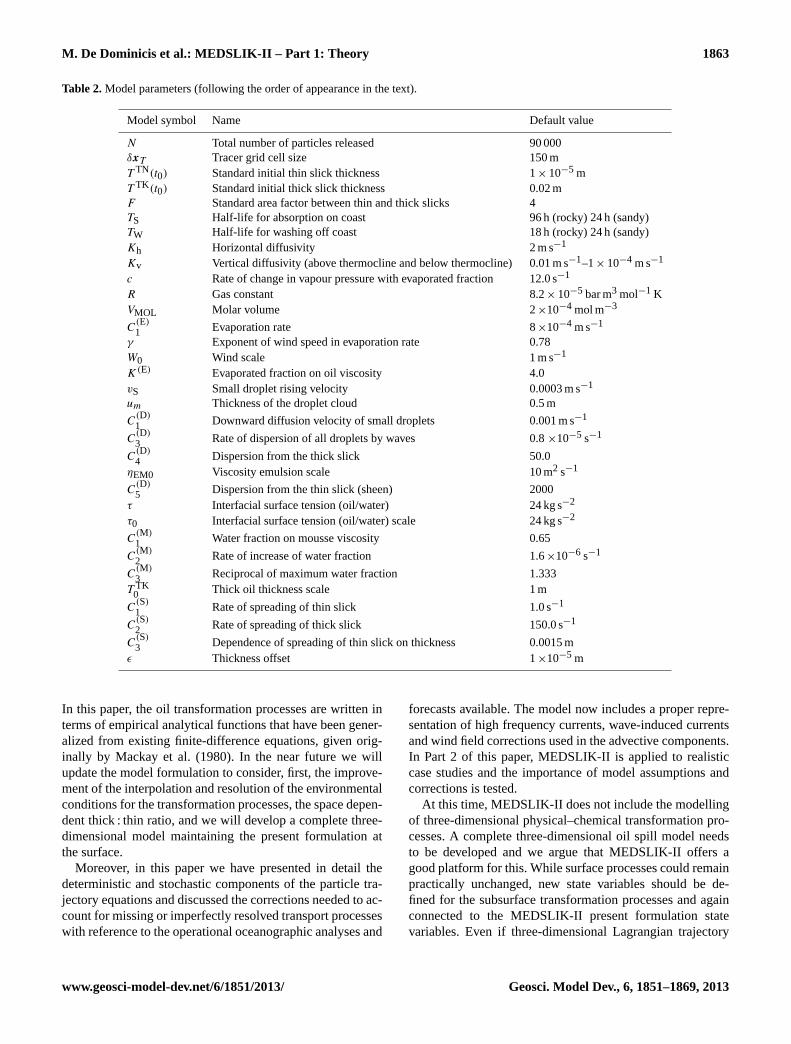
Table 2.Model parameters (following the order of appearance in the text).

Model symbol Name Default value

N Total number of particles released 90 000δxT Tracer grid cell size 150 mT TN(t0) Standard initial thin slick thickness 1× 10−5 mT TK(t0) Standard initial thick slick thickness 0.02 mF Standard area factor between thin and thick slicks 4TS Half-life for absorption on coast 96 h (rocky) 24 h (sandy)TW Half-life for washing off coast 18 h (rocky) 24 h (sandy)Kh Horizontal diffusivity 2 m s−1

Kv Vertical diffusivity (above thermocline and below thermocline) 0.01 m s−1–1× 10−4 m s−1

c Rate of change in vapour pressure with evaporated fraction 12.0 s−1

R Gas constant 8.2× 10−5 bar m3 mol−1 KVMOL Molar volume 2×10−4 mol m−3

C(E)1 Evaporation rate 8×10−4 m s−1

γ Exponent of wind speed in evaporation rate 0.78W0 Wind scale 1 m s−1

K(E) Evaporated fraction on oil viscosity 4.0vS Small droplet rising velocity 0.0003 m s−1

um Thickness of the droplet cloud 0.5 m

C(D)1 Downward diffusion velocity of small droplets 0.001 m s−1

C(D)3 Rate of dispersion of all droplets by waves 0.8×10−5 s−1

C(D)4 Dispersion from the thick slick 50.0

ηEM0 Viscosity emulsion scale 10 m2 s−1

C(D)5 Dispersion from the thin slick (sheen) 2000

τ Interfacial surface tension (oil/water) 24 kg s−2

τ0 Interfacial surface tension (oil/water) scale 24 kg s−2

C(M)1 Water fraction on mousse viscosity 0.65

C(M)2 Rate of increase of water fraction 1.6×10−6 s−1

C(M)3 Reciprocal of maximum water fraction 1.333

T TK0 Thick oil thickness scale 1 m

C(S)1 Rate of spreading of thin slick 1.0 s−1

C(S)2 Rate of spreading of thick slick 150.0 s−1

C(S)3 Dependence of spreading of thin slick on thickness 0.0015 m

ε Thickness offset 1×10−5 m

In this paper, the oil transformation processes are written interms of empirical analytical functions that have been gener-alized from existing finite-difference equations, given orig-inally by Mackay et al.(1980). In the near future we willupdate the model formulation to consider, first, the improve-ment of the interpolation and resolution of the environmentalconditions for the transformation processes, the space depen-dent thick : thin ratio, and we will develop a complete three-dimensional model maintaining the present formulation atthe surface.

Moreover, in this paper we have presented in detail thedeterministic and stochastic components of the particle tra-jectory equations and discussed the corrections needed to ac-count for missing or imperfectly resolved transport processeswith reference to the operational oceanographic analyses and

forecasts available. The model now includes a proper repre-sentation of high frequency currents, wave-induced currentsand wind field corrections used in the advective components.In Part 2 of this paper, MEDSLIK-II is applied to realisticcase studies and the importance of model assumptions andcorrections is tested.

At this time, MEDSLIK-II does not include the modellingof three-dimensional physical–chemical transformation pro-cesses. A complete three-dimensional oil spill model needsto be developed and we argue that MEDSLIK-II offers agood platform for this. While surface processes could remainpractically unchanged, new state variables should be de-fined for the subsurface transformation processes and againconnected to the MEDSLIK-II present formulation statevariables. Even if three-dimensional Lagrangian trajectory



equations have been used by different oceanographic com-munities, particular work will be required to adapt mod-elling assumptions to the specific oil transformation pro-cesses in the water column. This paper might offer the nec-essary detailed description of the present-day Lagrangianoil spill model assumptions so that the extension to three-dimensional marine oil dynamics and transformation will bepossible in the near future.

Appendix A

Oil density

The oil density depends on the oil type which is classified us-ing the American Petroleum Institute gravity, or API gravity,which is a measure of how heavy or light a petroleum liquidis compared to water. From API gravity it is possible to cal-culate oil density. The conversion from API to density firstrequires conversion to specific gravity:

SG=141.5

(API + 131.5). (A1)

The specific gravity can subsequently be converted to den-sity:

ρ = SGρW, (A2)

where ρW is the water density assumed to be equal to1026 kg m−3.

In MEDSLIK-II the density remains constant over time:temperature expansions and emulsification effects are notconsidered in the density calculation. Using this hypothesis,MEDSLIK-II concentrations are valid only for short-termforecasting and in the absence of abrupt changes of tempera-ture.

Appendix B

Time rate of change of oil slick state variables

B1 Evaporation

Evaporation changes the volume of the thick and thin partsof the slick, and is the major transformation process afterthe initial oil release at the surface. The volume of oil lostby evaporation is computed using Mackay’s algorithm forevaporation (Mackay et al., 1980). Given the assumption thattransformation processes are evaluated at the slick centre, thetime rate of change of the volume lost by evaporation fromthe thick slick,V TK , is expressed as

dV TK

dt

∣∣∣∣(E)

=dfTK

dt

∣∣∣∣(E)

[V TK(t0) + V TN(t0)

], (B1)

whereV TK(t0) andV TN(t0) are the initial thick and thin slick

volumes, respectively, anddfTKdt

∣∣∣(E)

is the time rate of change

of the fraction of oil evaporated. For the thick oil slick, thetime rate of change of the fraction of oil evaporated is

dfTK

dt

∣∣∣∣(E)

=P0e

−cfTK t

PoilKM

ATK

V TK (1− fTK) (B2)

and

Poil =RT

VMOL, (B3)

wherePoil (bar) is the oil vapour pressure,P0 is the ini-tial vapour pressure (which depends on the oil type used),c (s−1) is a constant that measures the rate of decrease ofvapour pressure with the fraction already evaporated,ATK(t)

is the area of the thick part of the slick,KM (m s−1) is theevaporative exposure to wind,T (K) is the temperature,R(bar m3 mol−1 K) is the gas constant andVMOL (mol m−3) isthe molar volume of the oil. ForKM we assume

KM = C(E)1 (3.6

W

W0)γ , (B4)

where WW0

is the non-dimensional 10 m wind modulus (W0 is

1 m s−1), γ is a constant, andC(E)1 (m s−1) is the evaporation

rate. The standard values ofc, R, VMOL , γ andC(E)1 are given

in Table2.For the thin slick oil, the time rate of change of the volume

is equal to

dV TN

dt

∣∣∣∣(E)

=dfTN

dt

∣∣∣∣(E)

[V TK(t0) + V TN(t0)

], (B5)

where dfTNdt

∣∣∣(E)

is the time rate of change of the oil fraction

evaporated from the thin slick.The evaporative component in the thin slick is assumed to

disappear immediately, but the thin slick, through the spread-ing process, is fed by oil from the thick slick that in generalhas not yet fully evaporated. Equating the oil content of thethin slick before and after the flow of oil coming from thethick slick, we obtain

dfTN

dt

∣∣∣∣(E)

=dV TN

dt

∣∣∣∣(S)

(fMAX − fTK)

V TN , (B6)

wherefMAX is the initial fraction of the evaporative compo-nent, which represents the maximum value that the oil frac-tion evaporated from the thin slick can attain. Evaporationleads to an increase in the viscosity of the oil, which is cal-culated using

η = η0eK(E)fTK , (B7)

whereη0 (m2 s−1) is the initial viscosity (which depends onthe oil type used) andK(E) is a constant that determines theincrease of viscosity with evaporation (see Table2).



B2 Dispersion

The oil dispersion processes occurring on an oil volume re-leased at the surface were framed in empirical formulas de-veloped byMackay et al.(1979). Wave action drives oil intothe water, forming a cloud of droplets beneath the spill. Thedroplets are classified as either large droplets that rapidly riseand coalesce again with the surface spill, or small dropletsthat rise more slowly, and may be immersed long enoughto diffuse into the lower water column layers. In the lattercase, they are lost from the surface spill and considered tobe permanently dispersed. The criterion that distinguishesthe small droplets is that their rising velocity under buoy-ancy forces is comparable to their diffusive velocity, whilefor large droplets the rising velocity is much larger.

The time rate of change of the thick slick volume due towater column dispersal of small droplets is given by

dV TK

dt

∣∣∣∣(D)

=1

2

(CD

1 − vS

)CSATK

+dXS

dt, (B8)

whereC(D)1 (m s−1) is the downward diffusive velocity of

the small droplets, andvS (m s−1) is the rising velocity of thesmall droplets.C(D)

1 andvS are constant parameters listed inTable2; cs is the fraction of the small droplets; andXs is thevolume of small droplets beneath the thick slick. The amountof small droplets is equal to

XS = CSumATK, (B9)

whereum (m) is the vertical thickness of the droplet cloud(see Table2). The large droplets are not regarded as dispersedsince they eventually re-coalesce with the slick. The fractionof the small droplets is calculated using the following expres-sion:

CS =

2C(D)3

(WW0

+ 1)2

T TKSTK

vS+ C(D)1

, (B10)

whereC(D)3 (s−1) is a constant which controls the rate of dis-

persion of all droplets by waves (see Table2), WW0

is the non-dimensional wind speed at the oil slick centre, andSTK isthe fraction of small droplets in the dispersed oil beneath thethick slick, equal to

STK =

[1+ C

(D)4

(ηEM

ηEM0

) 12(

T TK

10−3T TK0

)(τ

τ0

)]−1

,

(B11)

whereC(D)4 controls the fraction of droplets below a critical

size,τ is the interfacial surface tension between oil and wa-ter (kg s−2) andηEM (m2 s−1) is the emulsified oil viscositythat will be defined later. The standard values ofC

(D)4 , τ , τ0,

ηEM0, andT TK0 are listed in Table2. For the thin slick dis-

persion only small droplets are considered. It is assumed thatthese droplets are all lost from the surface spill at the follow-ing rate:

dV TN

dt

∣∣∣∣(D)

= C(D)3

(W

W0+ 1

)2

T TNATNSTN and (B12)

STN =

(1+ C

(D)5

τ

τ0

)−1

, (B13)

whereC(D)5 is control dispersion from the thin slick (see Ta-

ble 2), WW0

is the non-dimensional wind speed at the oil slickcentre andSTN is the fraction of small droplets in the dis-persed oil beneath the thin slick.

B3 Emulsification

Emulsification refers to the process by which water becomesmixed with the oil in the slick. The main effect of emulsifi-cation is to form a mousse with viscosityηEM given by

ηEM = ηexp

[2.5f W

1− C(M)1 f W

], (B14)

whereη is defined by Eq. (B7), f W is the fraction of waterin the oil-water mousse andC(M)

1 is a constant which con-trols the effect of water fraction on mousse viscosity (seeTable 2). Emulsification is assumed to continue untilηEMreaches a maximum valueηMAX corresponding to a moussecomposed of floating tar balls. Mackay’s model for the timerate of change off W is (Mackay et al., 1979)

df W

dt

∣∣∣∣(M)

= C(M)2

(W

W0+ 1

)2[1− C

(M)3 f W

], (B15)

where WW0

is the non-dimensional wind speed calculated at

the slick centre,C(M)2 (s−1) is a constant which controls

the rate of water absorption in the mousse andC(M)3 is a

constant which controls the maximum water fraction in themousse (see Table2).

According to Eqs. (B14) and (B15) emulsification influ-ences the mousse viscosity, which, in turn, influences disper-sion (see Eq.B11).

B4 Spreading

Spreading consists of two processes: the first is the area lostdue to oil converted from the thick to the thin slick and thesecond corresponds to Fay’s gravity-viscous phase of spread-ing (Al-Rabeh et al., 2000). The thin and thick slick volume



rates due to spreading are then written as

dV TK

dt

∣∣∣∣(S)

= −dV TN

dt

∣∣∣∣(S)

+ T TKFG and (B16)

dV TN

dt

∣∣∣∣(S)

= T TN dATN

dt

∣∣∣∣(S)

, (B17)

where FG is defined later and correspond to Fay’s gravityspreading. Mackay’s model (Mackay et al., 1979, 1980) ap-proximates the thin slick area increment by

dATN

dt

∣∣∣∣(S)

= C(S)1

(ATN)1/3(

T TK0

)4/3exp

(−C

(S)3

T TK + ε

), (B18)

whereC(S)1 (s−1) is the constant rate of spreading of the thin

slick, andC(S)3 (m) controls the dependence on thickness of

the spreading of the thin slick, andε is a constant parameter.C

(S)1 , C(S)

3 andε standard values are listed in Table2. For thethick slick, Fay’s spreading is assumed to be written as

FG= C(S)2

(ATK)1/3(

T TK)4/3, (B19)

whereC(S)2 (s−1) is a constant rate of spreading of the thick

slick (see Table2).The time rate of change of the area of the thick slick due

to spreading is

dATK

dt

∣∣∣∣(S)

=1

T TK

dV TK

dt

∣∣∣∣(S)

. (B20)

Mechanical spreading is considered to occur for an initialperiod of 48 h after the oil release or until the thickness of thethick part of the slick,T TK , determined by Eq. (35), becomesequal to that of the thin slick,T TN. If this occurs the modelterminates all further spreading and from that point the slickis modelled as a thin slick only.

Appendix C

Stokes drift

Stokes drift velocity is the difference between the averageLagrangian flow velocity of fluid particles and the averageEulerian flow velocity of the fluid at a fixed position (the av-erage is usually taken over one wave period). Stokes driftvelocity is given by (Stokes, 1847)

DS(ω,z) = a2ωkcosh[2k(Z + H)]

2sinh2(KH), (C1)

whereω is the angular frequency,k is the wave number,ais the wave amplitude andH is the depth of the ocean. Thehorizontal component of Stokes drift velocity,DS, for deep-water waves(H → ∞) is approximately

DS(ω,z) u ωka2e2kz. (C2)

As it can be seen, Stokes drift velocity is a nonlinear quan-tity in terms of wave amplitude, and it decays exponentiallywith depth.

In MEDSLIK-II, the Stokes drift calculation is based on adiscrete wave spectrum approach. We start from the follow-ing two expressions: the average of the wave spectrum,S, isequal to the variance of the surface displacement,ζ :⟨ζ 2⟩=

∫S(ω)dω, (C3)

and the wave energy is related to the variance of sea surfacedisplacement by

E = ρWg⟨ζ 2⟩=

1

2ρWga2, (C4)

where ρW is water density andg is gravity. Then, fromEqs. (C3) and (C4), we obtain the relation between the waveamplitude and wave spectrum:

a2= 2

⟨ζ 2⟩= 2

∞∫0

S(ω)dω. (C5)

Introducing Eq. (C5) into Eq. (C2), the Stokes drift formu-lation becomes

DS(z) = 2

∞∫0

ωk(ω)S(ω)e2k(ω)zdω. (C6)

The wave spectrum,S, to be introduced into Eq. (C6),can be calculated using empirical parameterizations, that de-scribe the wave spectrum as a function of wind speed. Wehave chosen to use the Joint North Sea Wave Project (JON-SWAP) spectrum parameterization (Hasselmann et al.,1973), taking the wind and fetch into account:

S(ω) =εg

ω5exp

[−

5

4

(ωP

ω

)4]γ r . (C7)

The parametersr, ε, ωp, γ, andφ were determined duringthe JONSWAP experiment and are expressed by the follow-ing formulae:

r = exp

[−

(ω − ωP )2

2φ2ω2P

]; ε = 0.076

(W2

Fg

)0.22

;

ωP = 22

(g2

FW

) 13

; γ = 3.3;andφ =

{0.07 ω ≤ ωP

0.09 ω ≥ ωP

(C8)

whereF is the fetch, which is the distance over which thewind blows with constant velocity, andW is the wind ve-locity intensity at 10 m over the sea surface. In practice, thefetch is calculated as the minimum distance between the oilslick centre and the coast in the opposite direction of the winddirection.



From the wave spectrum, the significant wave height canbe also calculated. It is defined as the average height of thehighest third of the waves, during a fixed sampling interval,and it can be written as

HS = 4

√∫S(ω)dω. (C9)

Appendix D

Technical specifications

The oil spill model code MEDSLIK-II is freely availableand can be downloaded together with the User Manual, testcase data and output example from the websitehttp://gnoo.bo.ingv.it/MEDSLIKII/. MEDSLIK-II is available under theGNU General Public License (Version 3, 29 June 2007).The code is written in Fortran77, Python and Shell script-ing. The model can run on any workstation and laptop. Thearchitecture currently supported is Linux (tested on Ubuntu10.04 LTS). The software requirements are a Fortran com-piler (gfortran is fully compatible) and NetCDF libraries.

Acknowledgements.This work was funded by MyOcean Projectand MEDESS4MS Project.

Edited by: D. Ham

References

Al-Rabeh, A. H., Lardner, R. W., and Gunay, N.: Gulfspill Version2.0: a software package for oil spills in the Arabian Gulf, Envi-ron. Modell. Softw., 15, 425–442, 2000.

Ambjörn, C.: Seatrack Web, Forecasts of Oil Spills, a New Version,Environ. Res. Eng. Manage., 3, 60–66, 2007.

ASA: OILMAP for Windows (technical manual), Narrangansett,Rhode Island: ASA Inc, 1997.

ASCE: State-of-the-Art Review of Modeling Transport and Fate ofOil Spills, J. Hydraulic Eng., 122, 594–609, 1996.

Berry, A., Dabrowski, T., and Lyons, K.: The oil spill model OIL-TRANS and its application to the Celtic Sea, Mar. Pollut. Bull.,64, 2489–2501, 2012.

Butenschön, M. and Zavatarelli, M., and Vichi, M.: Sensitivity ofa marine coupled physical biogeochemical model to time res-olution, integration scheme and time splitting method, OceanModel., 52, 36–53, 2012.

Carracedo, P., Torres-López, S., Barreiro, M., Montero, P., Balseiro,C., Penabad, E., Leitao, P., and Pérez-Muñuzuri, V.: Improve-ment of pollutant drift forecast system applied to the Prestige oilspills in Galicia Coast (NW of Spain): Development of an oper-ational system, Mar. Pollut. Bull., 53, 350–360, 2006.

Castanedo, S., Medina, R., Losada, I. J., Vidal, C., Mendez, F. J.,Osorio, A., Juanes, J. A., and Puente, A.: The Prestige oil spillin Cantabria Bay of Biscay). Part I: Operational forecasting sys-tem for quick response, risk assessment, and protection of naturalresources, J. Coast. Res., 22, 1474–1489, 2006.

Coppini, G., De Dominicis, M., Zodiatis, G., Lardner, R., Pinardi,N., Santoleri, R., Colella, S., Bignami, F., Hayes, D. R., Soloviev,D., Georgiou, G., and Kallos, G.: Hindcast of oil-spill pollutionduring the Lebanon crisis in the Eastern Mediterranean, July–August 2006, Mar. Pollut. Bullet., 62, 140–153, 2011.

Daniel, P., Marty, F., Josse, P., Skandrani, C., and Benshila, R.:Improvement of drift calculation in Mothy operational oil spillprediction system, in: International Oil Spill Conference (Van-couver, Canadian Coast Guard and Environment Canada), vol. 6,2003.

De Dominicis, M., Leuzzi, G., Monti, P., Pinardi, N., andPoulain, P.: Eddy diffusivity derived from drifter data for dis-persion model applications, Ocean Dynam., 62, 1381–1398,doi:10.1007/s10236-012-0564-2, 2012.

De Dominicis, M., Pinardi, N., Zodiatis, G., and Archetti, R.:MEDSLIK-II, a Lagrangian marine surface oil spill model forshort-term forecasting – Part 2: Numerical simulations and vali-dations, Geosci. Model Dev., 6, 1871–1888, doi:10.5194/gmd-6-1871-2013, 2013.

Griffa, A.: Applications of stochastic particle models to oceano-graphic problems, in: Stochastic modelling in physical oceanog-raphy, Progress in Probability, 39, 113–140, 1996.

Gurney, K., Law, R., Denning, A., Rayner, P., Baker, D., Bous-quet, P., Bruhwiler, L., Chen, Y. H., Ciais, P., Fan, S., Fung,I. Y., Gloor, M., Heimann, M., Higuchi, K., John, J., Maki,T., Maksyutov, S., Masarie, K., Peylin, P., Prather, M., Pak, B.C., Randerson, J., Sarmiento, J., Taguchi, S., Takahashi, T., andYuen, C.-W.: Towards robust regional estimates of CO2 sourcesand sinks using atmospheric transport models, Nature, 415, 626–630, 2002.

Gurney, K., Law, R., Denning, A., Rayner, P., Pak, B., Baker, D.,Bousquet, P., Bruhwiler, L., Chen, Y., Ciais, P., Fung, I. Y.,Heimann, M., John, J., Maki, T., Maksyutov, S., Peylin, P.,Prather, M., and Taguchi, S.: Transcom 3 inversion intercom-parison: Model mean results for the estimation of seasonal car-bon sources and sinks, Global Biogeochem. Cy., 18, GB1010,doi:10.1029/2003GB002111, 2004.

Hackett, B., Breivik, Ø., and Wettre, C.: Forecasting the Drift of Ob-jects and Substances in the Ocean, Ocean Weather Forecasting,Springer, Netherlands, 507–523, 2006.

Haidvogel, D. B. and Beckmann, A.: Numerical ocean circulationmodeling, Imperial College Pr, 318 pp., ISBN 9781860941146,1999.

Hasselmann, K., Barnett, T., Bouws, E., Carlson, H., Cartwright,D., Enke, K., Ewing, J., Gienapp, H., Hasselmann, D., Kruse-man, P., Meerburg, A., Mller, P., Olbers, D., Richter, K., Sell, W.,and Walden, H.: Measurements of wind-wave growth and swelldecay during the Joint North Sea Wave Project (JONSWAP),Ergänzungsheft zur Deutschen Hydrographischen ZeitschriftReihe, A8–12, 1973.

Huntley, H. S., Lipphardt, B. L., and Kirwan, A. D.: Surface driftpredictions of the Deepwater Horizon spill: The Lagrangian per-spective, in: Monitoring and Modeling the Deepwater Horizon




http://dx.doi.org/10.1007/s10236-012-0564-2

http://dx.doi.org/10.5194/gmd-6-1871-2013

http://dx.doi.org/10.5194/gmd-6-1871-2013

http://dx.doi.org/10.1029/2003GB002111


Oil Spill: A Record-Breaking Enterprise, Geophys. Monogr. Ser.,195, 179–195, 2011

Lardner, R., Zodiatis, G., Loizides, L., and Demetropoulos, A.:An operational oil spill model for the Levantine Basin (EasternMediterranean Sea), in: International Symposium on Marine Pol-lution, 1998.

Lardner, R., Zodiatis, G., Hayes, D., and Pinardi, N.: Applicationof the MEDSLIK Oil Spill Model to the Lebanese Spill of July2006, European Group of Experts on Satellite Monitoring of SeaBased Oil Pollution, European Communities, 2006.

Lehr, W., Jones, R., Evans, M., Simecek-Beatty, D., and Overstreet,R.: Revisions of the ADIOS oil spill model, Environ. Modell.Softw., 17, 189–197, 2002.

Lenn, Y. D. and Chereskin, T. K.: Observations of Ekman currentsin the Southern Ocean, J. Phys. Oceanogr., 39, 768–779, 2009.

Liu, Y., MacFadyen, A., Ji, Z.-G., and Weisberg, R. H.: Introductionto Monitoring and Modeling the Deepwater Horizon Oil Spill, in:Monitoring and Modeling the Deepwater Horizon Oil Spill: ARecord-Breaking Enterprise, Geophys. Monogr. Ser., 195, 1–7,2011a.

Liu, Y., Weisberg, R. H., Hu, C., and Zheng, L.: Trajectory fore-cast as a rapid response to the Deepwater Horizon oil spill, in:Monitoring and Modeling the Deepwater Horizon Oil Spill: ARecord-Breaking Enterprise, Geophys. Monogr. Ser., 195, 153–165, 2011b.

Lorimer, G.: The kernel method for air quality modelling– I, Math-ematical foundation, Atmos. Environ. (1967), 20, 1447–1452,1986.

Mackay, D., Buist, I., Mascarenhas, R., and Paterson, S.: Oil spillprocesses and models. Report to Research and Development Di-vision, Environment Emergency Branch, Environmental ImpactControl Directorate, Environmental Protection Service, Environ-ment Canada, Ottawa, 1979.

Mackay, D., Paterson, S., and Trudel, B.: A mathematical modelof oil spill behaviour, Report to Research and Development Di-vision, Environment Emergency Branch, Environmental ImpactControl Directorate, Environmental Protection Service, Environ-ment Canada, Ottawa, 1980.

Nittis, K., Perivoliotis, L., Korres, G., Tziavos, C., and Thanos, I.:Operational monitoring and forecasting for marine environmen-tal applications in the Aegean Sea, Environ. Modell. Softw., 21,243–257, 2006.

Noye, J.: Numerical methods for solving the transport equation,Num. Model. Application Mar. Syst., 145, 195–229, 1987.

Pedlosky, J.: The buoyancy and wind-driven ventilated thermocline,J. Phys. Oceanogr., 16, 1077–1087, 1986.

Pinardi, N. and Coppini, G.: Preface “Operational oceanography inthe Mediterranean Sea: the second stage of development”, OceanSci., 6, 263–267, doi:10.5194/os-6-263-2010, 2010.

Pinardi, N., Allen, I., Demirov, E., De Mey, P., Korres, G., Las-caratos, A., Le Traon, P.-Y., Maillard, C., Manzella, G., andTziavos, C.: The Mediterranean ocean forecasting system: firstphase of implementation (1998–2001), Ann. Geophys., 21, 3–20,doi:10.5194/angeo-21-3-2003, 2003.

Pollani, A., Triantafyllou, G., Petihakis, G., Nittis, K., Dounas, C.,and Christoforos, K.: The Poseidon operational tool for the pre-diction of floating pollutant transport, Mar. Pollut. Bull., 43, 270–278, 2001.

Price, J. F., Weller, R. A., and Schudlich, R. R.: Wind-driven oceancurrents and Ekman transport, Science, 238, 1534–1538, 1987.

Pugliese Carratelli, E., Dentale F., and Reale F.: On the effects ofwave-induced drift and dispersion in the Deepwater Horizon oilspill, in: Monitoring and Modeling the Deepwater Horizon OilSpill: A Record-Breaking Enterprise, Geophys. Monogr. Ser.,195, 197–204, 2011.

Reed, M., Gundlach, E., and Kana, T.: A coastal zone oil spillmodel: development and sensitivity studies, Oil Chem. Pollut.,5, 411–449, 1989.

Reed, M., Aamo, O. M., and Daling, P. S.: Quantitative analysisof alternate oil spill response strategies using OSCAR, Spill Sci.Technol. Bull., 2, 67–74, 1995.

Reed, M., Johansen, Ø., Brandvik, P. J., Daling, P., Lewis, A.,Fiocco, R., Mackay, D., and Prentki, R.: Oil Spill Modeling to-wards the Close of the 20th Century: Overview of the State ofthe Art, Spill Sci. Technol. Bull., 5, 3–16, 1999.

Risken, H.: The Fokker-Planck equation, Springer, 475 pp., ISBN354061530X, 9783540615309, 1989.

Röhrs, J., Christensen, K. H., Hole, L. R., Broström, G., Driv-dal, M., and Sundby, S.: Observation-based evaluation of surfacewave effects on currents and trajectory forecasts, Ocean Dynam-ics, 62, 10-12, 1519–1533, 2012.

Schreurs, P., Mewis, J., and Havens, J.: Numerical aspects of aLagrangian particle model for atmospheric dispersion of heavygases, J. Hazardous Materials, 17, 61–80, doi:10.1016/0304-3894(87)85042-2, 1987.

Shen, H. T., Yapa, P. D., and Petroski, M. E.: A Simulation Modelfor Oil Slick Transport in Lakes, Water Resour. Res., 23, 1949–1957, 1987.

Sibert, J. R., Hampton, J., Fournier, D. A., and Bills, P. J.: Anadvection-diffusion-reaction model for the estimation of fishmovement parameters from tagging data, with application toskipjack tuna (Katsuwonus pelamis), Canadian J. Fish. AquaticSci., 56, 925–938, 1999.

Sobey, R. J. and Barker, C. H.: Wave-driven transport of surface oil,J. Coastal Res., 13, 490–496, 1997.

Sotillo, M., Alvarez Fanjul, E., Castanedo, S., Abascal, A., Menen-dez, J., Emelianov, M., Olivella, R., García-Ladona, E., Ruiz-Villarreal, M., Conde, J., Gøomez, M., Conde, P., Gutierrez, A.,and Medina, R.: Towards an operational system for oil-spill fore-cast over Spanish waters: Initial developments and implementa-tion test, Mar. Pollut. Bull., 56, 686–703, 2008.

Spaulding, M., Kolluru, V., Anderson, E., and Howlett, E.: Applica-tion of three-dimensional oil spill model (WOSM/OILMAP) tohindcast the Braer spill, Spill Sci. Technol. Bull., 1, 23–35, 1994.

Stohl, A.: Computation, accuracy and applications of trajectories– A review and bibliography, Atmos. Environ., 32, 947–966,doi:10.1016/S1352-2310(97)00457-3, 1998.

Stokes, G.: On the theory of oscillatory waves, Transactions of theCambridge Philosophical Society, 8, 441–473, 1847.

Tompson, A. and Gelhar, L.: Numerical Simulation of Solute Trans-port in Three-Dimensional, Randomly Heterogeneous PorousMedia, Water Resour. Res., 26, 2541–2562, 1990.

Wang, J. and Shen, Y.: Development of an integrated model sys-tem to simulate transport and fate of oil spills in seas, Sci. ChinaTechnol. Sci., 53, 2423–2434, 2010.


http://dx.doi.org/10.5194/os-6-263-2010

http://dx.doi.org/10.5194/angeo-21-3-2003

http://dx.doi.org/10.1016/0304-3894(87)85042-2

http://dx.doi.org/10.1016/0304-3894(87)85042-2

http://dx.doi.org/10.1016/S1352-2310(97)00457-3


Wang, S., Shen, Y., Guo, Y., and Tang, J.: Three-dimensional nu-merical simulation for transport of oil spills in seas, Ocean Eng.,35, 503–510, 2008.

Woods, J.: Primitive equation modelling of plankton ecosystems,Ocean Forecasting, Conceptual Basis and Applications, editedby: Pinardi, N. and Woods, J., Springer-Verlag Berlin Heidel-berg, 2002.

Wunsch, C.: The work done by the wind on the oceanic generalcirculation, J. Phys. Oceanogr., 28, 2332–2340, 1998.

Zelenke, B., O’Connor, C., Barker, C., Beegle-Krause, C. J.,and Eclipse, L. (Eds.): General NOAA Operational ModelingEnvironment (GNOME) Technical Documentation, US Dept.of Commerce, NOAA Technical Memorandum NOS OR&R40. Seattle, WA: Emergency Response Division, NOAA, 105pp., available at:http://response.restoration.noaa.gov/gnome_manual, 2012.

Zodiatis, G., Lardner, R., Hayes, D., Georgiou, G., Pinardi, N., DeDominicis, M., and Panayidou, X.: The Mediterranean oil spilland trajectory prediction model in assisting the EU responseagencie, in: Congreso Nacional de Salvamento en la Mar, Cadiz,2–4 October, libro de actas, 535–547, 2008a.

Zodiatis, G., Lardner, R., Hayes, D. R., Georgiou, G., Sofianos,S., Skliris, N., and Lascaratos, A.: Operational ocean forecast-ing in the Eastern Mediterranean: implementation and evalua-tion, Ocean Sci., 4, 31–47, doi:10.5194/os-4-31-2008, 2008b.

Zodiatis, G., Lardner, R., Solovyov, D., Panayidou, X., and De Do-minicis, M.: Predictions for oil slicks detected from satellite im-ages using MyOcean forecasting data, Ocean Sci., 8, 1105–1115,doi:10.5194/os-8-1105-2012, 2012.


http://response.restoration.noaa.gov/gnome_manual

http://response.restoration.noaa.gov/gnome_manual

http://dx.doi.org/10.5194/os-4-31-2008

http://dx.doi.org/10.5194/os-8-1105-2012

medslik-ii, a lagrangian marine surface oil spill model for … · 2016-01-24 · conceptual...

Documents