medical image segmentation using weak priors
TRANSCRIPT

Research Collection
Doctoral Thesis
Medical Image Segmentation using Weak Priors
Author(s): Gass, Tobias
Publication Date: 2014
Permanent Link: https://doi.org/10.3929/ethz-a-010340283
Rights / License: In Copyright - Non-Commercial Use Permitted
This page was generated automatically upon download from the ETH Zurich Research Collection. For moreinformation please consult the Terms of use.
ETH Library
DISS. ETH NO. 22146
Medical Image Segmentationusing Weak Priors
A thesis submitted to attain the degree of
DOCTOR OF SCIENCES of ETH ZURICH(Dr. sc. ETH Zurich)
presented by
Tobias GassDipl.-Inform., RWTH Aachen University
born on 25.07.1979citizen of Germany
accepted on the recommendation of
Prof. Dr. Gábor Székely, examinerProf. Dr. Hans-Peter Meinzer, co-examiner
Prof. Dr. Orçun Göksel, co-examiner
2014


Abstract
Image segmentation is a core technique in medical image analysis. By enabling seman-tic interpretability of raw image data, it allows both medical experts and automatic pro-cessing software to diagnose and to plan for the treatment of pathologies with greateraccuracy and efficiency. An additional use-case for segmentations is to learn models ofanatomical variability, for example statistical shape models, which are an important toolin clinical workflows. Such models have been used to recognize diseases and injuries, todrive reconstructive surgery and patient-specific implant design, and in robust automaticsegmentation of anatomical structures.
One critical requirement for statistical shape models or similarly powerful segmentationmethods is their dependence on a large database of segmented images, which containsstrong prior knowledge about the organ and/or its shape. Such database then cannotbe built without human assistance, since most automatic segmentation methods requirestrong prior knowledge as said before. In order to break this vicious circle of mutual de-pendency, it is the goal of this thesis to investigate and develop reliable and accurate auto-matic segmentation methods which require only weak prior information such as a singleannotated image, or a database of unsegmented images to learn general prior knowledge.The following two main approaches are explored in this thesis.
First, a novel technique has been developed which allows for the simultaneous registrationof a single segmented image (atlas) to an unsegmented image, while also segmenting thelatter based on an intensity model. This approach enables the segmentation goal functionto be included into the registration criterion, while using the atlas as a weak shape prior.
The second approach utilizes the information contained in a set of unsegmented imagesto improve atlas-based segmentation. Motivated by semi-supervised techniques in ma-chine learning, three different algorithms have been developed. The first proposed tech-nique utilizes unsegmented images along with their automatic, atlas based segmentationsas weak atlases, which can then be used to generate additional segmentation hypothesesfor each unsegmented image. Such segmentation hypotheses are then fused analogouslyto multi-atlas segmentation methods. This was shown to greatly increase the accuracyand reliability of the atlas-based segmentation. Similarly, another technique has beenproposed to fuse registration hypotheses, which can be obtained either by running multi-ple registration algorithms/parametrizations or by composing registrations along indirect

ii
paths between images. The fusion of such registrations then optimizes a joint similarityand deformation smoothness criterion, and was shown to improve registration fidelity andatlas-based segmentation quality. Lastly, a novel algorithm has been developed whichaims at rectifying pair-wise non-rigid registrations by optimizing group-wise registrationconsistency, which previously has been used in the literature often for estimating the fi-delity of registration algorithms.
All methods have been experimentally evaluated on synthetic and clinical images fromdifferent modalities (CT and MR) and with different target structures (mandibular boneand Corpus Callosum). The fidelity of the resulting segmentations was demonstrated tobe improved consistently compared to other segmentation methods that use weak priors.Crucially, worst-case performance was seen to improve substantially, which facilitates thedeployment of automatic segmentation methods in scenarios without human supervision.

Zusammenfassung
Die Bildsegmentierung ist ein wichtiges Verfahren in der Analyse medizinischer Bilder.Sie erlaubt die semantische Interpretierbarkeit von Bild-Rohdaten und ermöglicht es da-durch sowohl medizinischen Experten als auch automatischer Software Pathologien mitgrösserer Genauigkeit und Effizienz zu diagnostizieren und zu behandeln. Segmentie-rungen können weiterhin benutzt werden um Modelle der anatomischen Variabilität zulernen. Solche Techniken, zum Beispiel statistische Formmodelle, sind wichtige Werk-zeuge in klinischen Prozessen. Ihr Anwendungsbereich reicht von der Erkennung vonKrankheiten und Verletzungen, über rekonstruirende Chirurgie und Implantat-Design, biszu robuster Segmentierung anatomischer Strukturen.
Eine essentielle Voraussetzung für die Berechnung statistischer Formmodelle oder ähn-lich mächtiger Segmentierungsmethoden ist das Vorhandensein einer umfangreichen Da-tenbank von segmentierten Bildern, welche starkes Vorwissen über ein Organ und seineForm enthält. Die Erstellung solch einer Datenbank muss dann mit Unterstützung durchmedizischine Experten erfolgen, da automatische Segmentierungsmethoden häufig aufdas starke Vorwissen einer solchen Datenbank angewiesen sind. Das Ziel dieser Arbeitwar es, dieses Abhängigkeitsverhältnis zu durchbrechen indem verlässliche und akku-rate Segmentierungsmethoden entwickelt werden, welche nur schwaches Vorwissen be-nötigen. Dieses kann beispielsweise von einem einzelnen segmentierten Bild, oder einerDatenbank von unsegmentierten Bildern gelernt beziehungsweise abgeleitet werden. Diefolgenden zwei Leit-Ansätze wurden in dieser Arbeit verfolgt.
Als Erstes wurde ein neuer Algorithmus entwickelt, der es ermöglicht ein Bild basie-rend auf einem Intensitätsmodell zu segmentieren und gleichzeitig ein einzelnes segmen-tiertes Bild (Atlas) nicht-linear zu registrieren. Dieser Ansatz erlaubt die Inklusion derSegmentierungs-Zielfunktion in die Registrierung, und damit die Verwendung des Atlasals schwaches Vorwissen über die Form.
Der zweite Ansatz verwendet die Information, die in einer Menge von unsegmentiertenBildern vorhanden ist, um Atlas-basierte Segmentierung zu verbessern. Motiviert durchsemi-supervised learning in maschinellem Lernen wurden drei unterschiedliche Algo-rithmen entwickelt. Die erste Methode verwendet unsegmentierte Bilder zusammen mitihrer automatischen, Atlas-basierenden Segmentierung als schwache Atlasse. Diese kón-nen dann benutzt werden um zusätzliche Segmentierungs-Hypothesen zu generieren, wel-

iv
che dann analog zu Multi-Atlas Segmentierungsmethoden kombiniert werden können,was die Verlässlichkeit und Genauigkeit der Segmentierung stark verbessert. Ähnlich da-zu kombiniert der zweite Algorithmus Verformungs-Hypothesen, welche durch mehrfa-ches Ausführen von unterschiedlichen Registrierungs-Methoden oder Parametrisierun-gen, oder durch die Komposition von Registrierungen über indirekte Pfade zwischenBildern berechnet werden können. Diese Hypothesen werden in dem vorgeschlagenemAlgorithmus durch die Optimierung eines Kriteriums fusioniert, welches Bildähnlichkeitund Verformungsglattheit kombiniert. Die berechneten Verformungen resultieren in ver-besster Registrierungs- und Atlas-basierender Segmentierungsqualität. Zuletzt wurde einneuer Algorithmus entwickelt, welcher zum Ziel hat paar-weiser nichtlinearer Registrie-rungen zu Rektifizieren indem die Konsistenz der Registrierungen in einer Gruppe vonBildern optimiert wird.
Alle Methoden wurden experimentell auf synthetischen und klinischen Daten unterschied-licher Modalität (CT und MR), und mit unterschiedlichen Zielorganen (Kieferknochenund Corpus Callosum) validiert und evaluiert. Es konnte gezeigt werden dass die Qualitätder resultierenden Segmentierungen konsistent besser ist als andere Segmentierungsver-fahren die schwaches Vorwissen verwenden. Entscheidenderweise konnte die Qualitätder schlechtesten Resultate substantiell verbessert werden, was den Einsatz von automa-tischen Segmentierungsmethoden in Szenarien ohne menschliche Kontrolle vereinfacht.
Acknowledgments
First and foremost, I would like to express my gratitude to Prof. Gábor Székely, who hasgiven me the opportunity to explore the exciting field of medical image analysis as part ofthe Computer Vision Lab at ETH Zurich. His support and confidence in my work, alongwith many interesting discussions and valuable feedback, has shaped not only this thesisbut also my relationship with this field of research. I would also like to thank Prof. Hans-Peter Meinzer, who has kindly agreed to review this thesis and to serve as committeemember of my doctoral defense. Many thanks also to Dr. Remi Blanc, who supervised meduring the beginning of my thesis and helped to set the path for this work. Furthermore, Iwant to express my profound gratitude to Prof. Orçun Göksel for his advice, never-endingvigor, enthusiasm and support in countless productive meetings and collaborative work.
I also owe gratitude to the CO-ME network, which has created a fantastic environmentfor scientific research and exchange. In addition to funding the research in this thesisas part of the Swiss NCCR CO-ME, it provided invaluable opportunities to network andcollaborate.
I would like to thank Thomas Deselaers and Henning Mueller for introducing me to (med-ical) computer vision and nurturing my interest in research.
Many thanks also to my colleagues at the Computer Vision Lab, who made the chal-lenging task of stumbling towards scientific merit (and/or the PhD degree) enjoyable. Inparticular, I would like to thank my ’extended office’ mates Fabian, Valeria, Henning,Severin, Rasmus and Marko for entertainment, advice, enough coffee and creating anoverall fun atmosphere.
I want to thank my parents for being great examples in being curious, open, confident andhappy, and motivating and enabling me, among a lot of things, to strive for a PhD degree. Iwant to thank my brother for all the games we played, sports we learned, fights we foughtand adventures we shared. My grandparents for being everything I can imagine wantingthem to be, and passing on their love for the mountains, which is one of the reasons Iwent to Switzerland. Finally, I am incredibly grateful for the chance to explore, enjoy andshare life with Charlotte.
Contents
1 Introduction 11.1 Semi-Automatic Segmentation . . . . . . . . . . . . . . . . . . . . . . . 21.2 Automatic Segmentation . . . . . . . . . . . . . . . . . . . . . . . . . . 3
1.2.1 Priors in Automatic Segmentation . . . . . . . . . . . . . . . . . 31.2.1.1 Appearance Priors . . . . . . . . . . . . . . . . . . . . 41.2.1.2 Shape Priors . . . . . . . . . . . . . . . . . . . . . . . 51.2.1.3 Combined Priors . . . . . . . . . . . . . . . . . . . . . 5
1.2.2 Semi-Supervised Segmentation . . . . . . . . . . . . . . . . . . . 61.3 Goals . . . . . . . . . . . . . . . . . . . . . . . . . . . . . . . . . . . . 71.4 Contributions and Organization . . . . . . . . . . . . . . . . . . . . . . . 8
2 Auxiliary Anatomical Labels for Joint Segmentation and Non-RigidAtlas Registration 112.1 Introduction . . . . . . . . . . . . . . . . . . . . . . . . . . . . . . . . . 122.2 Method . . . . . . . . . . . . . . . . . . . . . . . . . . . . . . . . . . . 13
2.2.1 Joint Registration and Segmentation . . . . . . . . . . . . . . . . 142.2.2 Auxiliary Labels . . . . . . . . . . . . . . . . . . . . . . . . . . 15
2.2.2.1 Coherence Potentials foe Auxiliary Labels . . . . . . . 162.3 Experimental Evaluation . . . . . . . . . . . . . . . . . . . . . . . . . . 16
2.3.1 Discussion . . . . . . . . . . . . . . . . . . . . . . . . . . . . . . 182.4 Conclusions . . . . . . . . . . . . . . . . . . . . . . . . . . . . . . . . . 19
3 Simultaneous Segmentation and Multi-Resolution Nonrigid AtlasRegistration 213.1 Introduction . . . . . . . . . . . . . . . . . . . . . . . . . . . . . . . . . 223.2 Background and Notation . . . . . . . . . . . . . . . . . . . . . . . . . . 263.3 Simultaneous Registration and Segmentation . . . . . . . . . . . . . . . 283.4 Implementation using Markov Random Fields . . . . . . . . . . . . . . . 30
3.4.1 Two-Layer Graph . . . . . . . . . . . . . . . . . . . . . . . . . . 313.4.2 SRS using a Multi-Resolution Framework . . . . . . . . . . . . . 323.4.3 Algorithm . . . . . . . . . . . . . . . . . . . . . . . . . . . . . . 35
3.4.3.1 Potential Functions . . . . . . . . . . . . . . . . . . . . 353.4.4 Implementation of ARS . . . . . . . . . . . . . . . . . . . . . . 37
3.5 Experimental Evaluation . . . . . . . . . . . . . . . . . . . . . . . . . . 383.6 Discussion . . . . . . . . . . . . . . . . . . . . . . . . . . . . . . . . . . 453.7 Conclusions . . . . . . . . . . . . . . . . . . . . . . . . . . . . . . . . . 49
4 Semi-supervised Segmentation Using Multiple Segmentation Hy-potheses from a Single Atlas 514.1 Introduction . . . . . . . . . . . . . . . . . . . . . . . . . . . . . . . . . 514.2 Label Propagation . . . . . . . . . . . . . . . . . . . . . . . . . . . . . . 534.3 Compact Graphs . . . . . . . . . . . . . . . . . . . . . . . . . . . . . . . 544.4 Results and Discussion . . . . . . . . . . . . . . . . . . . . . . . . . . . 554.5 Conclusions . . . . . . . . . . . . . . . . . . . . . . . . . . . . . . . . . 59
5 Registration Fusion using Markov Random Fields 615.1 Introduction . . . . . . . . . . . . . . . . . . . . . . . . . . . . . . . . . 615.2 Registration Fusion using an MRF . . . . . . . . . . . . . . . . . . . . . 63
5.2.1 MRegFuse with Folding Removal (MRegFuseR) . . . . . . . . . . . 655.2.2 Pair-wise and Population-Based Registration Fusion . . . . . . . . 66
5.3 Experimental Results . . . . . . . . . . . . . . . . . . . . . . . . . . . . 675.3.1 Discussion . . . . . . . . . . . . . . . . . . . . . . . . . . . . . . 70
5.4 Conclusions . . . . . . . . . . . . . . . . . . . . . . . . . . . . . . . . . 71
6 Consistency-Based Rectification of Non-Rigid Registrations 736.1 Introduction . . . . . . . . . . . . . . . . . . . . . . . . . . . . . . . . . 746.2 Notation and Background . . . . . . . . . . . . . . . . . . . . . . . . . . 776.3 Method . . . . . . . . . . . . . . . . . . . . . . . . . . . . . . . . . . . 78
6.3.1 CBRR Algorithm: Consistency . . . . . . . . . . . . . . . . . . . 796.3.2 CBRR Algorithm: Prior . . . . . . . . . . . . . . . . . . . . . . 806.3.3 Casting into a System of Linear Equations . . . . . . . . . . . . . 816.3.4 Iterative Refinement . . . . . . . . . . . . . . . . . . . . . . . . 836.3.5 Implementation . . . . . . . . . . . . . . . . . . . . . . . . . . . 83
6.4 Experimental Results . . . . . . . . . . . . . . . . . . . . . . . . . . . . 846.4.1 Synthetic Images . . . . . . . . . . . . . . . . . . . . . . . . . . 846.4.2 2D MR Images . . . . . . . . . . . . . . . . . . . . . . . . . . . 866.4.3 3D CT Segmentation . . . . . . . . . . . . . . . . . . . . . . . . 896.4.4 4D Liver MRI Motion Estimation . . . . . . . . . . . . . . . . . 926.4.5 Discussion . . . . . . . . . . . . . . . . . . . . . . . . . . . . . . 92
6.5 Conclusions . . . . . . . . . . . . . . . . . . . . . . . . . . . . . . . . . 96
7 Summary and Perspectives 97
Bibliography 101
viii
List of Figures
1.1 Data requirements and examples for strong and weak priors . . . . . . . . 31.2 Vicious circle for robust automatic segmentation . . . . . . . . . . . . . . 7
2.1 Auxiliary-label joint segmentation and registration . . . . . . . . . . . . . 132.2 Pipeline for obtaining the auxiliary-labelled atlas segmentation . . . . . . 162.3 Progression of coherence potential . . . . . . . . . . . . . . . . . . . . . 172.4 Example segmentations of the corpus callosum . . . . . . . . . . . . . . 182.5 Effect of coherence potential weight on single- and aux-label ARS. . . . . 19
3.1 A synthetic example comparing SRS to traditional methods . . . . . . . . 223.2 Product-label SRS vs. our sum-label SRS . . . . . . . . . . . . . . . . . 233.3 Bayesiean network and factor graph for the SRS MAP problem . . . . . . 293.4 Schematic of a local pixel neighborhood in the SRS MRF defined on the
pixel level . . . . . . . . . . . . . . . . . . . . . . . . . . . . . . . . . . 313.5 Illustration of the SRS-MRF using different resolutions for registration
and segmentation subgraphs . . . . . . . . . . . . . . . . . . . . . . . . 333.6 Progression of the SRS algorithm on a 2D MRI corpus callosum segmen-
tation task . . . . . . . . . . . . . . . . . . . . . . . . . . . . . . . . . . 343.7 Minimizing one instance of the SRS energy using α-expansion graph-cuts
and TRW-S. . . . . . . . . . . . . . . . . . . . . . . . . . . . . . . . . . 383.8 Deformed segmentation SA(T )and segmentation estimate SX for single-
label SRS and multi-label SRS. . . . . . . . . . . . . . . . . . . . . . . . 413.9 Sample segmentations using the different approaches . . . . . . . . . . . 423.10 Distribution of the results for mandibular bone and CC l1o experiments . 443.11 Results of all the methods on five different examples . . . . . . . . . . . . 453.12 Facial feature tracking example in a video sequence . . . . . . . . . . . . 46
4.1 Illustration of standard atlas based segmentation and our proposed method 534.2 Sample results for both datasets . . . . . . . . . . . . . . . . . . . . . . . 564.3 Segmentation accuracy (Dice) of traditional single atlas based segmenta-
tion and our proposed method with LAW fusion for each atlas and targetimage combination . . . . . . . . . . . . . . . . . . . . . . . . . . . . . 57
4.4 Dice metric for support sample selection for a single atlas using randomselection, GSW-based, individual ARE, and ARE-G ranking criteria . . . 58
ix
5.1 Schematic of the proposed MRF fusion . . . . . . . . . . . . . . . . . . . 635.2 Unary potentials for MRegFuse . . . . . . . . . . . . . . . . . . . . . . . 655.3 Population-based registration hypotheses generation . . . . . . . . . . . . 665.4 Example fusion result for independently computed registrations . . . . . . 685.5 Two registration examples showing the Jacobian determinant values for
MRegFuse and MRegFuseR . . . . . . . . . . . . . . . . . . . . . . . . . . 695.6 Regularization and folding in MRegFuse . . . . . . . . . . . . . . . . . . . 70
6.1 (a) Group-wise registration to the mean image (center), implicitly imply-ing complete consistency via the inferred inter-image registrations (dashed).CBRR utilises the information from the complete set of pair-wise registra-tions (b). In this set, it aims at reducing the registration inconsistency bymodifying pair-wise transformations such that the differences ~r betweendirect and indirect transformations are minimised (c). This is done simul-taneously for all pair-wise transformations using all possible registrationtriplets. This allows us to exploit the redundant information from multipleloops for each transformation (d). . . . . . . . . . . . . . . . . . . . . . . 76
6.2 Inconsistency and target registration error (TRE) for registration loops in4D liver MRI sequences. Each point indicates the inconsistency of oneloop of three registrations and the average TRE of those three registra-tions, and the blue line is a least-square fit with r=0.77 denoting the Pear-son correlation. For more details on the data and registration algorithmsplease see Sec. 6.4.4. . . . . . . . . . . . . . . . . . . . . . . . . . . . . 79
6.3 Local normalized cross correlation (LNCC) weight used for the CBRRregularizer. Shown are target image, deformed source, and LNCC weightcomputed with σ = 4 mm and γ = 10 for sample pairs from the MRI(top) and CT (bottom) datasets. . . . . . . . . . . . . . . . . . . . . . . 80
6.4 Relative improvement using CBRR on synthetic data using random ground-truth deformations of varying complexity, additive random errors withvariable magnitude and frequency, and varying CBRR grid resolution. . . 86
6.5 Data generation for the 2D MR experiment. First, image X1 is registeredto the remaining images Xi, resulting in transformations T1,i (top left).Then, X1 is deformed using the estimated transformation and 50% SNRGaussian noise (ζ) is added, generating new images X ′i (top right). Pair-wise transformations Ti,j between all X ′i are known analytically throughthe registrations from X1. The image set X1, X
′2, . . . , X
′N is then used
as the experimental dataset and the known dense correspondences Ti,j asthe ground-truth in evaluation. . . . . . . . . . . . . . . . . . . . . . . . 87
6.6 Relative ATE improvement using CBRR with an increasing number of 2DMR images. Each experiment is repeated 10 times with randomly selectedimages. The standard deviation of the results is shown by the error bars. . 88
6.7 Right: Improvements through CBRR over multiple iterations. . . . . . . . 89

6.8 CBRR of MRF (top) and demons (bottom) registration on the 2D MRIdata. Shown are from left to right: target image, deformed source, trueregistration error, error of rectified registration and the source image de-formed by the rectified registration. The hue of the color in the errorvisualizations indicates its orientation, while the saturation correspondsto the error magnitude. . . . . . . . . . . . . . . . . . . . . . . . . . . . 90
6.9 Surface distance of ground-truth jawbone segmentation to MRF-registeredsource (left) and subsequent CBRR (right). Best viewed in color. . . . . . 90
6.10 Segmentation overlap percentiles on the 3D CT dataset. Each datapointshows the maximum Dice coefficient for a given percentage of the 210total pair-wise registrations. . . . . . . . . . . . . . . . . . . . . . . . . . 91
6.11 Inconsistency and TRE of one loop of sequence1 before and after usingCBRR for the PTV registration method. Mid-sagittal slices are shownfor MRIs, inconsistency, and TRE extrapolated using thin-plate splines.CBRR was computed on a longer sequence using 11 images and 110 reg-istrations in total. . . . . . . . . . . . . . . . . . . . . . . . . . . . . . . 93
6.12 TRE before and after CBRR on the 4D Liver MRI sequences. Each pointshows the error for a single landmark before (x-axis) and after (y-axis)CBRR. Note that points blow the y = x line indicate a reduction in errorusing CBRR. . . . . . . . . . . . . . . . . . . . . . . . . . . . . . . . . 94
6.13 Mid-coronal slices of the mean images of the 3D CT dataset for (a) group-wise and (b) CBRR registration. For CBRR, one image was chosen asreference to which all images were aligned for averaging. We deformedthe group-wise mean to the same image to allow a better comparison. . . . 94
List of Tables
2.1 Segmentation results for joint segmentation and registration . . . . . . . . 17
3.1 Evaluation datasets . . . . . . . . . . . . . . . . . . . . . . . . . . . . . 393.2 Parameters for the different experimetns . . . . . . . . . . . . . . . . . . 393.3 Average segmentation quality metrics in the 3D CT mandibular bone seg-
mentation task . . . . . . . . . . . . . . . . . . . . . . . . . . . . . . . . 403.4 Average segmentation quality metrics in the 2D MR corpus callosum seg-
mentation task . . . . . . . . . . . . . . . . . . . . . . . . . . . . . . . . 433.5 Landmark registration error (mm) on the CC . . . . . . . . . . . . . . . . 43
xi
4.1 Mean segmentation accuracy from leave-one-out evaluation on the MR(2D) and CT (3D) datasets. . . . . . . . . . . . . . . . . . . . . . . . . . 57
5.1 Results using independently computed registrations and their fusion . . . 675.2 Fusing registrations obtained by automatic hypothesis generation in sets
of mutually registered images . . . . . . . . . . . . . . . . . . . . . . . . 69
6.1 Left: Average transformation error (ATE), inconsistency C and pearsoncorrelation ρ of estimated and true registration error magnitude for the 2DMRI experiments using simulated transformations before and after usingCBRR. We also compare CBRR to locally averaged weighting (LWA), anearlier version of this work (CLERC) presented in [Gass et al., 2014c],and AQUIRC [Datteri and Dawant, 2012], which computes a dimension-less estimate of registration error which can be correlated with the trueerror. . . . . . . . . . . . . . . . . . . . . . . . . . . . . . . . . . . . . . 88
6.2 Quantitative evaluation of CBRR and comparison to group-wise registra-tion on the 3D CT dataset. Mean TRE, mean surface distance (MSD),Hausdorff distance (HD) and inconsistency C are given in mm. . . . . . . 91
6.3 Quantitative evaluation of CBRR on the 4D liver MRI sequences. The av-erage run time is the average time required to process one of the sequenceswith 11 breathing phases of 3D MR. . . . . . . . . . . . . . . . . . . . . 93

1Introduction
Imaging has become an invaluable tool in medical workflow by enabling non-invasivemapping of subject anatomies. In order to maximize the utility of image data, it is oftenimperative to semantically interpret the images, for example by delineating organs. Typi-cal imaging technologies only allow for the extraction of low-level semantic information,e.g. the local radiation absorption in computer tomography (CT). While some imagingresponses can be clearly identified (e.g. air in CT), the appearance of organs is often onlyunique with respect to the tissue which leads to ambiguities when discriminating betweenorgans of a similar tissue type, e.g. bones or muscles. An additional challenge is that mostimaging technologies require a trade-off between image quality versus imaging time (e.g.in MR) and radiation exposure (e.g. in CT). Consequently, low resolution and low signal-to-noise-ratio further impair the interpretability of medical images.
In order to facilitate semantic interpretation of medical images, one of the most importanttechniques is the segmentation of such images. Here, a segmentation is a partition of animage into (typically disjunct) regions. Such partitions can then be labeled according totheir anatomical or functional characteristics, thereby enabling a semantic interpretationof the data. This then opens up a multitude of possibilities of further processing andanalysis in clinical scenarios. For diagnosis, a segmentation can for example be used tomeasure brain athropy which is an indicator for Alzheimers disease [Scahill et al., 2002].Segmentations also enable many treatment procedures, where one of the most widely de-ployed techniques is organ delineation for radiotherapy (RT) planning [Pekar et al., 2004].While this is done mostly manually by an expert, a visualization of the surrounding or-gans and the tumor can help in guiding the planning to avoid tissue damage [Bondiauet al., 2005]. A rich database of segmented organs can also be used for further automaticanalysis of appearance and morphology. For instance, automatically trained appearancemodels can then be used to detect tumors or aid automatic segmentation methods. Fur-thermore, statistical models of organ shapes can be inferred, leading to a wide range ofpossible applications: Given a pathological case (for example due to trauma or malforma-tion), the most similar normal organ can be computed and used for reconstructive surgeryor implant design [Zachow et al., 2005]. It also allows for the estimation of 3D shapesfrom 2D images [Kurazume et al., 2009], which can reduce the radiation exposure of
2 1. INTRODUCTION
patients. Furthermore, statistical shape models are widely used in automatic segmenta-tion methods [Heimann and Meinzer, 2009] due to their adherence to anatomical priorknowledge.
1.1 Semi-Automatic Segmentation
Due to the critical nature of medical procedures for the well-being of patients, all stepsin such workflows should be as accurate as possible. For the segmentation of medicalimages, this has traditionally led to a high dependency on human experts, who are trainedwell and have the necessary prior knowledge on both the anatomical and the imagingside. A critical aspect of such manual segmentation is the availability and cost of timespent by an experienced clinician to annotate images. In order to alleviate this burden,several semi-automatic techniques have been developed to assist an expert in performingthis task. Aside from directly drawing a segmentation on the image or directly manipu-lating a template surface [McInerney and Terzopoulos, 1999], one of the most commonmethods in this context is region growing [Hojjatoleslami and Kittler, 1998], where a usersets an adaptive threshold that is used to label connected regions. A refinement then typ-ically facilitates connecting multiple such regions allowing for labeling anatomies withinhomegeneous intensities. An advanced method is grab-cut [Rother et al., 2004], wherea user labels distinctive foreground and background pixels. These labels are then used totrain generative appearance models for foreground and background, and a Markov ran-dom field (MRF) is used to find a spatially coherent segmentation. This segmentation isthen used as new initial labels and the process is repeated until convergence.
The cost associated with human-expert based segmentation methods limits the availabilityof advanced medical procedures to a broader range of patients [Olabarriaga and Smeul-ders, 2001]. Additionally, such segmentations are hardly ever objective, and significantvariability in segmentation results has been found in both intra- and inter-rater compari-son studies [Pizer et al., 1990, Fontana et al., 1993, Udupa, 1997, Yamamoto et al., 1999].Furthermore, clinical segmentations are often performed with a specific goal or tech-nology in mind, limiting their generalization capabilities. For instance, a segmentationoutline meant to be used for radiotherapy (RT) targeting can be adjusted based on theprior knowledge of the clinician with regards to characteristic of the RT beam and theknown/assumed locations of cancer, e.g. such that margins are wide around such criticalsegmentation borders. This means that such label might be originally intended to de-lineate a specific organ, but is altered in practice with the intended goal of RT in mind.This limits its generalizability, prohibiting the usage in different scenarios as for examplelearning of organ appearance. A further complication in human-assisted segmentationis that current computer systems mostly visualize 3D anatomies as 2D renderings. Thisleads to a tedious and error prone process when relying on human feedback, where it isfor example still very common that segmentations are performed on a slice-by-slice basis.
1.2. AUTOMATIC SEGMENTATION 3
Inferred from Example
Stro
ngpr
ior
Statistical shape model
Wea
kpr
ior
and(or)
Atlas registration
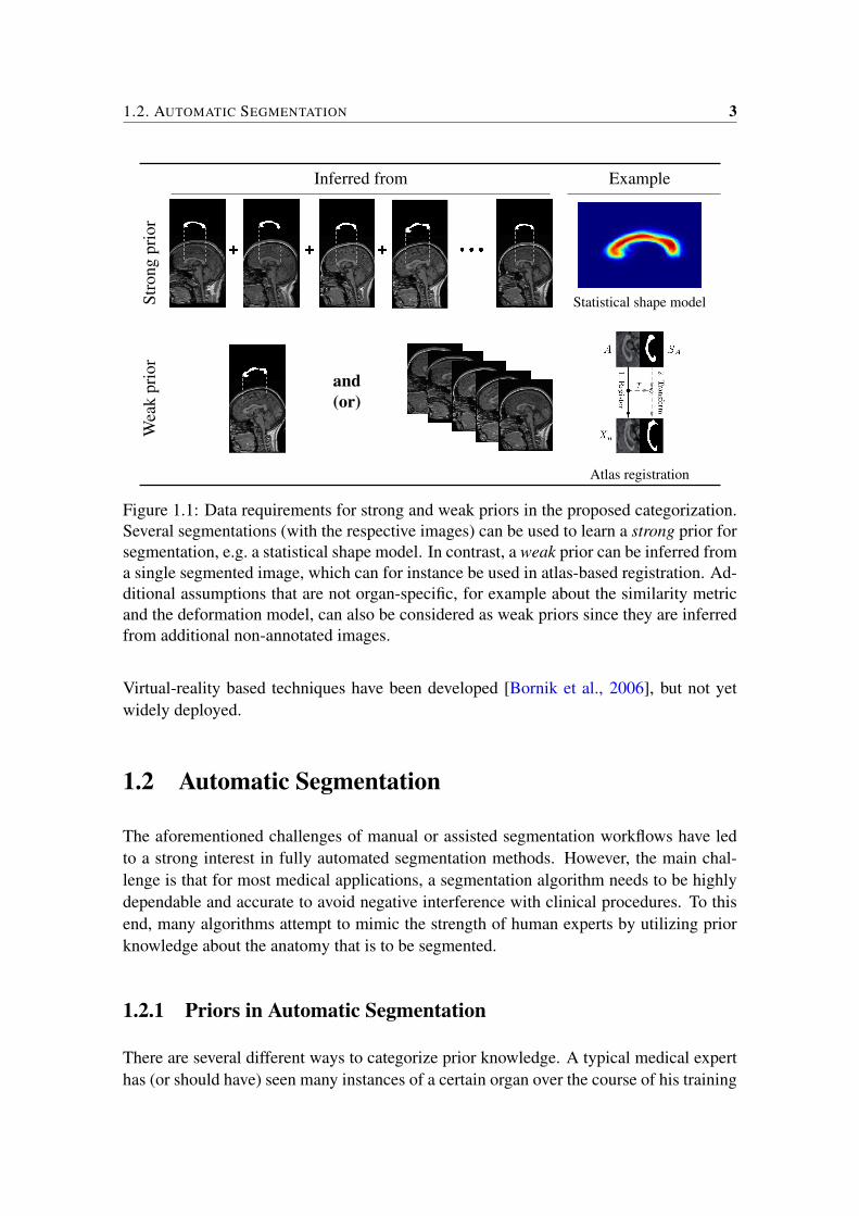
Figure 1.1: Data requirements for strong and weak priors in the proposed categorization.Several segmentations (with the respective images) can be used to learn a strong prior forsegmentation, e.g. a statistical shape model. In contrast, a weak prior can be inferred froma single segmented image, which can for instance be used in atlas-based registration. Ad-ditional assumptions that are not organ-specific, for example about the similarity metricand the deformation model, can also be considered as weak priors since they are inferredfrom additional non-annotated images.
Virtual-reality based techniques have been developed [Bornik et al., 2006], but not yetwidely deployed.
1.2 Automatic Segmentation
The aforementioned challenges of manual or assisted segmentation workflows have ledto a strong interest in fully automated segmentation methods. However, the main chal-lenge is that for most medical applications, a segmentation algorithm needs to be highlydependable and accurate to avoid negative interference with clinical procedures. To thisend, many algorithms attempt to mimic the strength of human experts by utilizing priorknowledge about the anatomy that is to be segmented.
1.2.1 Priors in Automatic Segmentation
There are several different ways to categorize prior knowledge. A typical medical experthas (or should have) seen many instances of a certain organ over the course of his training

4 1. INTRODUCTION
in at least one imaging modality, and potentially also observed it directly during surgery oras anatomical or histological specimen. This enables such expert to form an expectation ofthe typical shape and appearance of the organ, along with an expectation of the variabilityof these parameters. Analogously, algorithms can learn prior knowledge from annotateddata automatically. For the purpose of this thesis, prior knowledge which is similar tothe knowledge of an expert will be denominated as a strong prior, as it is inferred froma population of organ-specific samples. In contrast, a weak prior is then either organ-specific or population-based. This means that it can for instance be inferred from a singleinstance of the organ (organ-specific) or from a population of images without annotation.Fig. 1.1 visualizes the above-mentioned prior concept and gives examples of segmentationmethods which use such priors.
It is further possible to differentiate priors by their type, where appearance and shape aredistinctive characteristics, which will be explained in the following sections.
1.2.1.1 Appearance Priors
The term “appearance” is most commonly used in computer vision to describe features ofthe intensity distribution of an image. Herein, it will be used to denote the features thatsupport the intended segmentation of an organ or anatomical structure. A typical weakappearance prior is for example an intensity value used for thresholding [Fu and Mui,1981]. A noteable application for this is the segmentation of cortical bone in CT, wheresuch bone typically has the highest X-ray absorption rate and therefore appears as thebrightest structure in images. Note that such prior is then unspecific with regard to bone(as prosthesis and teeth may appear even brighter) or regard to a particular bone, and thuscan be considered weak in the proposed categorization.
More sophisticated appearance models for example based on support vector machines [Corteset al., 1995, Ricci and Perfetti, 2007] or random forests [Breiman, 2001, Lempitsky et al.,2009] are typically learned from a collection of pre-annotated images and can thereforebe categorized as strong priors. Due to the amount and variety of information captured,e.g. texture or local shape, such classifiers can then be targeted more specifically at indi-vidual organs. One of the crucial drawbacks of such methods is that they typically treateach pixel in the image independent of all others. This local approach is therefore highlysusceptible to noise or inhomogeneous appearance. These challenges can be alleviatedby incorporating spatial context in the segmentation method. Here, one general assump-tion is that appearance should be homogeneous within image regions, and inhomegeneousbetween them [Fu and Mui, 1981]. Such spatial context can again be general, anatomy-unspecific and therefore weak, as for example, employed in MRF-segmentation [Boykovand Jolly, 2000] in which a first-order Markov assumption encourages solutions that arepair-wise constant. Such pair-wise terms can also be adapted to favor boundaries betweenthe target object and background, where it is then common to learn such terms from popu-lations of images in conditional random field (CRF) approaches [Lafferty et al., 2001,Lee
1.2. AUTOMATIC SEGMENTATION 5
et al., 2005], which is thus considered here to use a strong prior. Alternative methodslearn appearance with spatial context using random forests [Criminisi et al., 2011].
1.2.1.2 Shape Priors
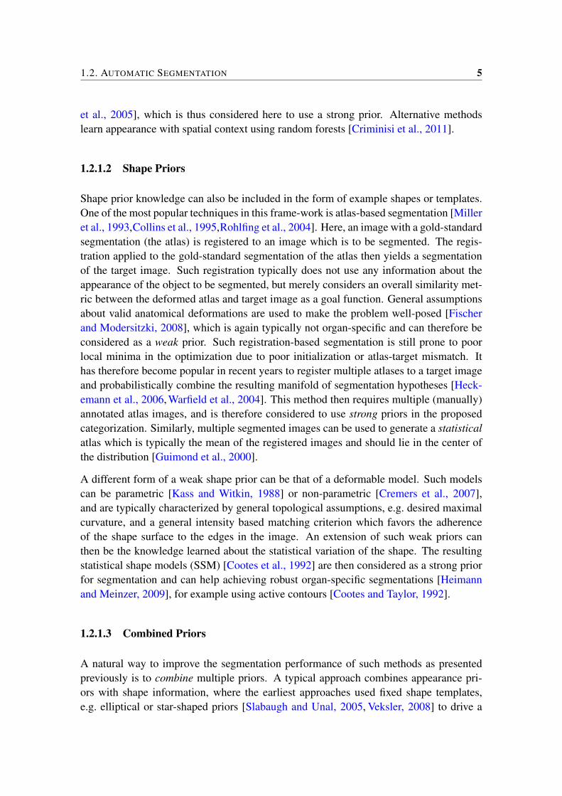
Shape prior knowledge can also be included in the form of example shapes or templates.One of the most popular techniques in this frame-work is atlas-based segmentation [Milleret al., 1993,Collins et al., 1995,Rohlfing et al., 2004]. Here, an image with a gold-standardsegmentation (the atlas) is registered to an image which is to be segmented. The regis-tration applied to the gold-standard segmentation of the atlas then yields a segmentationof the target image. Such registration typically does not use any information about theappearance of the object to be segmented, but merely considers an overall similarity met-ric between the deformed atlas and target image as a goal function. General assumptionsabout valid anatomical deformations are used to make the problem well-posed [Fischerand Modersitzki, 2008], which is again typically not organ-specific and can therefore beconsidered as a weak prior. Such registration-based segmentation is still prone to poorlocal minima in the optimization due to poor initialization or atlas-target mismatch. Ithas therefore become popular in recent years to register multiple atlases to a target imageand probabilistically combine the resulting manifold of segmentation hypotheses [Heck-emann et al., 2006, Warfield et al., 2004]. This method then requires multiple (manually)annotated atlas images, and is therefore considered to use strong priors in the proposedcategorization. Similarly, multiple segmented images can be used to generate a statisticalatlas which is typically the mean of the registered images and should lie in the center ofthe distribution [Guimond et al., 2000].
A different form of a weak shape prior can be that of a deformable model. Such modelscan be parametric [Kass and Witkin, 1988] or non-parametric [Cremers et al., 2007],and are typically characterized by general topological assumptions, e.g. desired maximalcurvature, and a general intensity based matching criterion which favors the adherenceof the shape surface to the edges in the image. An extension of such weak priors canthen be the knowledge learned about the statistical variation of the shape. The resultingstatistical shape models (SSM) [Cootes et al., 1992] are then considered as a strong priorfor segmentation and can help achieving robust organ-specific segmentations [Heimannand Meinzer, 2009], for example using active contours [Cootes and Taylor, 1992].
1.2.1.3 Combined Priors
A natural way to improve the segmentation performance of such methods as presentedpreviously is to combine multiple priors. A typical approach combines appearance pri-ors with shape information, where the earliest approaches used fixed shape templates,e.g. elliptical or star-shaped priors [Slabaugh and Unal, 2005, Veksler, 2008] to drive a
6 1. INTRODUCTION
MRF-based segmentation. In order to enable improved organ-specific segmentations,such general templates were replaced by shape models derived from aligned trainingshapes [Leventon et al., 2000, Rousson and Paragios, 2002, Ali et al., 2007]. In theseapproaches, the shape model is aligned to an image to be segmented which allows for pe-nalizing unlikely shapes. To overcome the often limited generalizability of SSMs alone,they are often used as regularizers, for example, by spatially constraining a graph-cutbased segmentation [Majeed et al., 2012]. In that work, a shape model can also be re-fitted using information from graph-cut segmentation and the process can be iterated untilconvergence. Alternatively, it is also possible to learn the statistical spatial variation ofthe appearance in combination with the variability of the shape. Such active appearancemodels (AAM, [Cootes et al., 2001]) combine a strong appearance model learned fromthe training population with a strong shape prior in the form of a statistical shape model.
1.2.2 Semi-Supervised Segmentation
Besides such priors learned from annotated images as detailed in the previous sections,semi-supervised learning is a thriving research domain, which originated in the machinelearning community [Chapelle et al., 2006]. Its underlying idea is to utilize the informa-tion that is contained in unlabeled samples for augmenting any other given prior knowl-edge.
In medical imaging, such information about shape and appearance can be obtained byanalyzing groups of images and introduce high-level assumptions about the relations ofthe images in this group. These assumptions are often general, and not anatomy-specificand can therefore be categorized as weak priors. For example, it can be assumed thatan anatomical structure to be segmented should have similar appearance across multipleimages. This assumption can then be used to co-segment two or more images by trainingforeground/background appearance models on both images jointly which is expected toincrease robustness [Rother et al., 2006,Han et al., 2011]. Since intensities alone are rarelya sufficient information cue for medical image segmentation, it is often required that theimages are brought into correspondence such that corresponding voxels then should havethe same segmentation label across all images. Two main approaches have been developedto achieve this goal: Joint segmentation and registration, pioneered by [Wyatt and Noble,2003], aims at improving both registration and segmentation by modeling them as a jointprocess. This work has inspired a large body of literature, which extends the originallyrigid, MRF-based technique to different non-rigid registration methods [Mahapatra andSun, 2012], variational segmentation methods [Ghosh et al., 2010], or additional bias fieldcorrection [Pohl et al., 2005]. While the original approach of [Wyatt and Noble, 2003]was formulated for any number of images, most of the joint segmentation and registrationapproaches focus on pairs of images.
1.3. GOALS 7
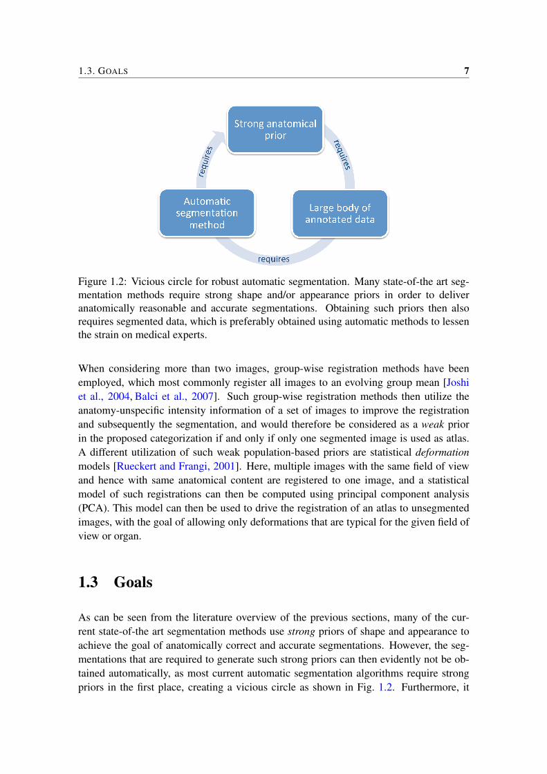
Figure 1.2: Vicious circle for robust automatic segmentation. Many state-of-the art seg-mentation methods require strong shape and/or appearance priors in order to deliveranatomically reasonable and accurate segmentations. Obtaining such priors then alsorequires segmented data, which is preferably obtained using automatic methods to lessenthe strain on medical experts.
When considering more than two images, group-wise registration methods have beenemployed, which most commonly register all images to an evolving group mean [Joshiet al., 2004, Balci et al., 2007]. Such group-wise registration methods then utilize theanatomy-unspecific intensity information of a set of images to improve the registrationand subsequently the segmentation, and would therefore be considered as a weak priorin the proposed categorization if and only if only one segmented image is used as atlas.A different utilization of such weak population-based priors are statistical deformationmodels [Rueckert and Frangi, 2001]. Here, multiple images with the same field of viewand hence with same anatomical content are registered to one image, and a statisticalmodel of such registrations can then be computed using principal component analysis(PCA). This model can then be used to drive the registration of an atlas to unsegmentedimages, with the goal of allowing only deformations that are typical for the given field ofview or organ.
1.3 Goals
As can be seen from the literature overview of the previous sections, many of the cur-rent state-of-the art segmentation methods use strong priors of shape and appearance toachieve the goal of anatomically correct and accurate segmentations. However, the seg-mentations that are required to generate such strong priors can then evidently not be ob-tained automatically, as most current automatic segmentation algorithms require strongpriors in the first place, creating a vicious circle as shown in Fig. 1.2. Furthermore, it

8 1. INTRODUCTION
was frequently observed that strong priors do not generalize well over different popu-lations [Blezek and Miller, 2007, Blanc et al., 2009], thus furthering the need for large,diverse bodies of segmented data from which to generate population-specific priors. It isthe goal of this thesis to develop efficient automatic methods for segmenting groups ofimages, such that the resulting data can then be used to break such vicious circle, i.e. as aset of annotations to build strong priors from. The developed segmentation methods willthus not use any form of strong priors, since such information for most anatomies do notexist or require large amounts of time to obtain by means of manual annotation.
1.4 Contributions and Organization
To achieve the aforementioned goals, the approaches investigated in this thesis focus onatlas-based segmentation, where such atlas is to be registered non-rigidly to an unseg-mented image with the purpose of transferring the atlas segmentation onto the target. Thischoice is motivated by the fact that such atlas-based segmentation can achieve reasonablesegmentation quality even with a limited, weak prior in the form of only a single atlasimage with segmentation annotation. It is, however, well-known that image registration istremendously difficult. Even if images are noise-free, and correspondences between im-ages exist, the widely used intensity based registration goal functions are only surrogatemeasures of registration quality, which leads to an ill-posed problem. The inclusion ofspatial regularization then results in an NP-complete elastic matching problem [Keysersand Unger, 2003], which makes it impossible to guarantee globally optimal solutions us-ing typical polynomial time registration algorithms. This thesis therefore aims at develop-ing algorithms to alleviate these challenges in non-rigid registration. Two main directionsare then investigated:
1. As far as segmentation is concerned, the non-rigid registration is only a means to anend, with the goal function only indirectly related to the actual segmentation goal.It is thus investigated to which extent the inclusion of a segmentation criterion inthe pair-wise registration goal function can benefit both the registration and thesegmentation targets.
2. This thesis also investigates means to explicitly utilize the information containedin the group of un-segmented images. In the spirit of semi-supervised learning,methods that can utilize such information to improve the segmentation of all imagesin a set using only weak priors are developed.
Specifically, the contributions presented in the thesis, and subsequently the structure ofthis manuscript, are as follows:

1.4. CONTRIBUTIONS AND ORGANIZATION 9
In the next two chapters, a novel method for simultaneous segmentation and non-rigidatlas registration using discrete optimization is developed. Chapter 2 focuses on the prob-lem of weak appearance priors for segmentation, which can lead to ill-posedness of jointregistration and segmentation (JRS). An algorithm is proposed that iterates between reg-istering the atlas and segmenting the target image, while penalizing the difference be-tween target segmentation and deformed atlas segmentation using a novel distance-basedpenalty in a discrete optimization framework. In order to deal with the ambiguity of theweak intensity prior, which is learned from the atlas image and segmentation, the JRSmodel is augmented by an auxiliary segmentation label which corresponds to tissue withthe same appearance as the target anatomy, e.g. other bone when a specific bone should besegmented. Chapter 3 then utilizes these techniques, but further develops a truly simulta-neous optimization of segmentation and registration in contrast to the alternating solutionof the previous chapter. A fundamental challenge of such simultaneous optimization isthe different levels of detail in which segmentation and registration are commonly solved,with segmentation being estimated at pixel-level and registration being commonly esti-mated based on a coarse grid of control points. To overcome this, a novel two-layerMarkov Random-Field (MRF) algorithm is proposed, where the structure is justified by arigorous probabilistic analysis of the underlying Bayesian optimization problem.
Chapter 4 then investigates a semi-supervised segmentation strategy where each unseg-mented image is first segmented by regular atlas-based segmentation, and then utilized asa weak atlas which can be used to generate additional segmentation hypotheses for theremaining unsegmented images. This results in several segmentation estimates for eachimage, which are fused analogously to multi-atlas segmentation. In the straight-forwardimplementation, a quadratic number of registrations is required, registering each imageto all remaining images. To overcome this computational burden, a support-sample se-lection strategy is devised which enables the automatic selection of a limited number ofunsegmented images as weak atlases in linear time, thus reducing the number of requiredadditional registrations.
Chapter 5 extends this concept to registrations, in contrast to segmentations as in theprevious chapter. Here, compositions of registrations along indirect paths between twoimages are used to generate additional registration hypotheses. Since no sound method tofuse such multiple registrations existed yet, a novel registration fusion method is devel-oped which allows for the joint optimization of an image similarity criterion and defor-mation smoothness in a discrete optimization framework. This general method can alsobe used to fuse registrations obtained in other settings as the group-wise scenario, for ex-ample, running different registration methods or parametrizations. This can alleviate theselection of the most appropriate registration algorithm or parametrization for new dataor application scenarios.
While the registration fusion presented in the previous chapter focuses on registrationsmoothness and post-registration image similarity, a novel registration post-processingmethod based on registration consistency is proposed in Chapter 6. Such consistency re-

10 1. INTRODUCTION
flects the assumption that correspondences should generally exist not only between imagepairs, but also between all images in a set of images. This criterion has been frequentlyused to quantify the quality of a registration algorithm, but had not yet been used as a goalfunction to be optimized within groups of images. In order to tackle the challenging opti-mization task of finding consistent correspondences between all images in a set of images,the problem is formulated as a registration post-processing step and it is cast as a linearleast-squares optimization problem, for which efficient algorithms exist. The resultingconsistent registrations are shown to improve not only the dense registration accuracy,but also the pair-wise post-registration segmentation overlap between the segmentationestimate and the ground-truth.
The thesis is concluded by a summary in Chapter 7, which briefly compares the proposedtechniques and gives an outlook on possible further research.
Chapters 2-5 have been published in peer-reviewed journals and conference proceedingsas [Gass et al., 2014a] [Gass et al., 2014e] [Gass et al., 2012] [Gass et al., 2014d]. Chapter6 is currently under review as [Gass et al., 2014b]. A preliminary version of the work inChapter 6 has been presented in [Gass et al., 2014c].

2Auxiliary Anatomical Labels for JointSegmentation and Non-Rigid AtlasRegistration
This paper studies improving joint segmentation and registration by introducing auxil-iary labels for anatomy that has similar appearance to the target anatomy while not beingpart of that target. Such auxiliary labels help avoid false positive labelling of non-targetanatomy by resolving ambiguity. A known registration of a segmented atlas can helpidentify where a target segmentation should lie. Conversely, segmentations of anatomy intwo images can help them be better registered. Joint segmentation and registration is thena method that can leverage information from both registration and segmentation to helpone another. It has received increasing attention recently in the literature. Often, merely asingle organ of interest is labelled in the atlas. In the presense of other anatomical struc-tures with similar appearance, this leads to ambiguity in intensity based segmentation; forexample, when segmenting individual bones in CT images where other bones share thesame intensity profile. To alleviate this problem, we introduce automatic generation of ad-ditional labels in atlas segmentations, by marking similar-appearance non-target anatomywith an auxiliary label. Information from the auxiliary-labeled atlas segmentation is thenincorporated by using a novel coherence potential, which penalizes differences betweenthe deformed atlas segmentation and the target segmentation estimate. We validated thison a joint segmentation-registration approach that iteratively alternates between register-ing an atlas and segmenting the target image to find a final anatomical segmentation. Theresults show that automatic auxiliary labelling outperforms the same approach using a sin-gle label atlasses, for both mandibular bone segmentation in 3D-CT and corpus callosumsegmentation in 2D-MRI.
This chapter has been published as: Gass, T., Szekely, G., and Goksel, O. (2014a). Auxiliary Anatom-ical Labels for Joint Segmentation and Atlas Registration. In Proc. SPIE Medical Imaging, volume 9034,page 90343T
12 2. AUXILIARY ANATOMICAL LABELS FOR JRS
2.1 Introduction
In computer vision, in general, and medical imaging, in particular, the segmentation ofan image is a common problem that has been studied extensively in the literature. Pos-sible approaches can be categorized by the amount of prior knowledge they use, suchas intensity-based segmentation on the one end of the spectrum and model-based seg-mentation on the other. Intensity-based segmentation typically involves a local classifierto determine the type of tissue that a pixel most likely belongs to. It can additionallyregularize such segmentation, for example using Markov random fields (MRF) [Boykovand Funke-Lea, 2006]. This method is typically fast, but lacks anatomical correctnessas neither absolute nor relative spatial locations (e.g., shapes) are taken into account.Due to its weak dependency on manual annotations, many recent studies have focusedon registration-based segmentation [Glocker et al., 2008] where a single reference (at-las) image is registered to a target image. The resulting transformation is then applied tothe labelled atlas, which yields a segmentation of the target image. While being widelyused in medical imaging, image registration alone cannot solve the segmentation task byitself as it is known to be an ill-posed problem [Fischer and Modersitzki, 2008]. Thisis because anatomical correspondences, which are not guaranteed to exist, are computedusing surrogate criteria such as intensity similarity. In addition, the problem of non-rigid registration is known to be NP-complete [Keysers and Unger, 2003], thus makingapproximative algorithms prone to local optima, for example due to poor initialization.Increasing the amount of prior knowledge is a common remedy for such problems, forexample by including multiple or statistical atlases [Rohlfing et al., 2005, Heckemannet al., 2006, Glocker et al., 2007].
In order to alleviate such problems, joint optimization of segmentation and registrationwas first proposed by [Wyatt and Noble, 2003]. Such methods allow segmentation andregistration processes to mutually benefit from one another. On the one hand, knowing thesegmentation of both target and atlas images one can greatly improve their registration.On the other hand, knowing the perfect correspondences between such two images willimprove, and even solve completely, the (atlas-based) segmentation problem. Accord-ingly, several approaches for such joint registration and segmentation have been proposedin the literature, focusing on alternating registration and segmentation (ARS) methods.
An ARS approach that alternates between estimating a rigid deformation using Powells’method and updating the segmentation using iterative conditional modes (ICM) in anMRF was proposed in [Wyatt and Noble, 2003]. Another approach based on MRFs thatalternates between solving one MRF to optimize registration parameters and to updatesegmentation probabilities, and a second MRF to solve the segmentation itself was intro-duced in [Xiaohua et al., 2004]. A Bayesian framework to alternate between updatingthe registration and estimating intensity “nuisance” parameters while marginalizing overpossible anatomical labels using an EM algorithm was presented in [Pohl et al., 2005].There have also been studies on alternating registration and segmentation in variational
2.2. METHOD 13
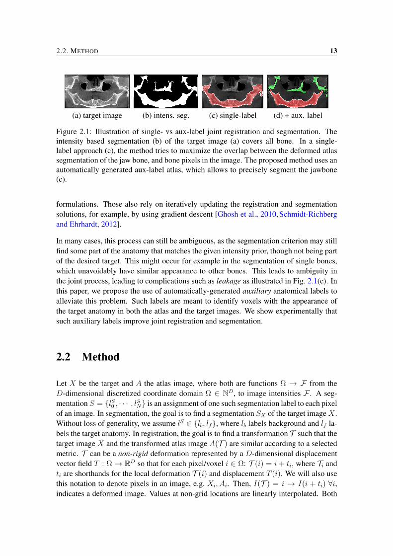
(a) target image (b) intens. seg. (c) single-label (d) + aux. label
Figure 2.1: Illustration of single- vs aux-label joint registration and segmentation. Theintensity based segmentation (b) of the target image (a) covers all bone. In a single-label approach (c), the method tries to maximize the overlap between the deformed atlassegmentation of the jaw bone, and bone pixels in the image. The proposed method uses anautomatically generated aux-label atlas, which allows to precisely segment the jawbone(c).
formulations. Those also rely on iteratively updating the registration and segmentationsolutions, for example, by using gradient descent [Ghosh et al., 2010, Schmidt-Richbergand Ehrhardt, 2012].
In many cases, this process can still be ambiguous, as the segmentation criterion may stillfind some part of the anatomy that matches the given intensity prior, though not being partof the desired target. This might occur for example in the segmentation of single bones,which unavoidably have similar appearance to other bones. This leads to ambiguity inthe joint process, leading to complications such as leakage as illustrated in Fig. 2.1(c). Inthis paper, we propose the use of automatically-generated auxiliary anatomical labels toalleviate this problem. Such labels are meant to identify voxels with the appearance ofthe target anatomy in both the atlas and the target images. We show experimentally thatsuch auxiliary labels improve joint registration and segmentation.
2.2 Method
Let X be the target and A the atlas image, where both are functions Ω → F from theD-dimensional discretized coordinate domain Ω ∈ ND, to image intensities F . A seg-mentation S = lS0 , · · · , lSN is an assignment of one such segmentation label to each pixelof an image. In segmentation, the goal is to find a segmentation SX of the target imageX .Without loss of generality, we assume lS ∈ lb, lf, where lb labels background and lf la-bels the target anatomy. In registration, the goal is to find a transformation T such that thetarget image X and the transformed atlas image A(T ) are similar according to a selectedmetric. T can be a non-rigid deformation represented by a D-dimensional displacementvector field T : Ω→ RD so that for each pixel/voxel i ∈ Ω: T (i) = i + ti, where Ti andti are shorthands for the local deformation T (i) and displacement T (i). We will also usethis notation to denote pixels in an image, e.g. Xi, Ai. Then, I(T ) = i → I(i + ti) ∀i,indicates a deformed image. Values at non-grid locations are linearly interpolated. Both

14 2. AUXILIARY ANATOMICAL LABELS FOR JRS
finding a displacement vector field T and a segmentation SX can be defined as separateenergy minimization problems as follows:
SX = arg minSX
∑i∈Ω
ψsegi (lSi ) +
∑j∈N (i)
λijsegΨsegij
(lSi , l
Sj
) (2.1)
T = arg minT
∑i∈Ω
ψregi (lRi ) +
∑j∈N (i)
λregΨregij (lRi , l
Rj )
, (2.2)
where N (i) denotes the neighbors of a pixel i and ψ,Ψ are unary and pairwise potentialfunctions, and λ are weights. The solutions ensure a smooth labelling of the image and canbe found efficiently using graph-based methods such as α-expansion graphcuts [Boykovet al., 2001]. We follow standard approaches for both segmentation and registration, usingHounsfield-unit based segmentation potentials as described in [Furnstahl et al., 2008] forbone segmentation in CT, and learned potential functions in the case of brain MR data. Forthe registration process, we follow the approach of [Glocker et al., 2008], with normalizedcross-correlation as the image similarity metric.
2.2.1 Joint Registration and Segmentation
As a joint technique, we implement an alternating registration and segmentation(ARS)procedure similar to [Wyatt and Noble, 2003]. In ARS, the estimated solution for onesubproblem is used as prior knowledge in the other in an iterative manner.
Using MRF approaches for both segmentation and non-rigid registration, we define anadditional energy that links the deformed atlas segmentation and the target segmentation,namely coherence energy Ecoh(SX , SA(T )). We compute this energy using a distanceweighted overlap penalty between the target segmentation and the deformed atlas seg-mentation as follows:
Ecoh(SA, SX , T ) =∑i
(1− δ(lSi , SA(Ti)))Ψcoh(lRi , lSi ) (2.3)
Ψcoh(lRi , lSi ) =
DlSi (Ti)2
2τ 2, (2.4)
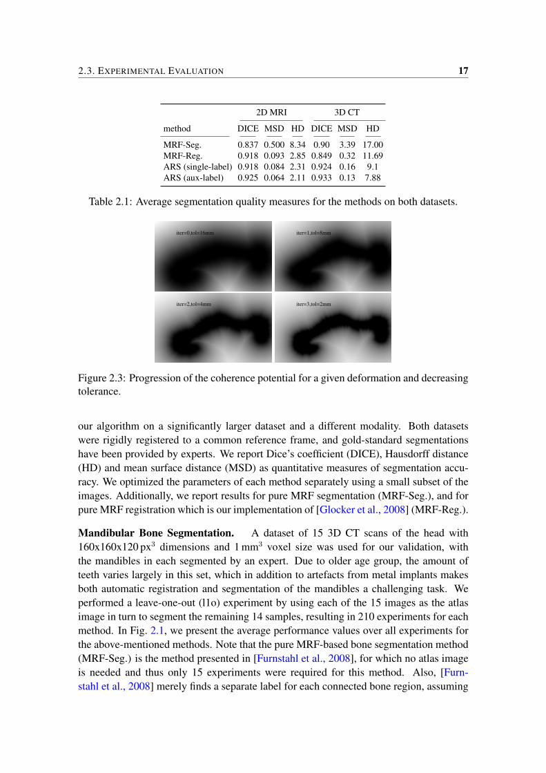
where δ is the Kronecker-delta, DlSi denotes the distance transform of SA with respect tolabel lSi and τ is a tolerance parameter, which we decrease after each ARS iteration, start-ing from an empirically-set tolerance of 16mm as can be seen in Fig. 2.3. This decrease intolerance was motivated by the fact that the expected difference between deformed atlassegmentation and target segmentation is larger in earlier levels compared to later stages.In experiments, a small tolerance in early levels was observed to undesirably force thetarget segmentation to be grossly dissimilar from the true segmentation, which in turn

2.2. METHOD 15
leads to a local optimum in the iterative registration process. This was mitigated by theabove-mentioned adaptive setting.
The ARS algorithm then alternates between estimating the registration and the segmenta-tion as follows:
T n+1 = arg minTEreg(X,A, T ) + λcohE
coh(SA, SnX , T )) (2.5)
Sn+1X = arg max
SX
Eseg(X,SX) + λcohEcoh(SA, SX , T
n+1), (2.6)
where λcoh weights the influence of the coherence energy, which is included in the MRFbased solver as a unary potential. Note that in the first iteration, no estimate of the seg-mentation is known and a regular registration is computed. We check for convergence bycomputing the overlap between Sn and Sn−1. The algorithm exits, if this overlap reaches99% or a maximum of 10 iterations is reached.
2.2.2 Auxiliary Labels
Naturally, any criterion similar to Ecoh(SX , SA(T )) will favor a high overlap between asingle-label atlas segmentation and any pixels which satisfy an intensity model for thisanatomy. This may lead to a sub-optimal solution in the joint registration and segmenta-tion process, where the atlas segmentation is forced to overlap with non-target anatomypixels. An example is given in Fig. 2.1, where the mandibular bone is extended into theskull. While this effect may partly be mitigated by strong regularization, this would thennot only deteriorate results in regions where high flexibility is necessary, but also couldmake the algorithm more sensitive to initialization.
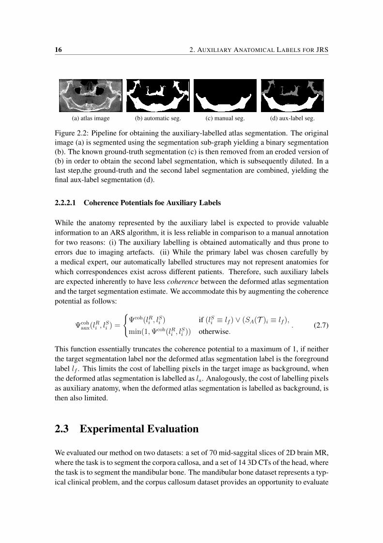
We thus propose auxiliary anatomical labels in both the atlas and the target segmentationin order to prevent such false positives in ARS segmentation. Such auxiliary labels canbe obtained automatically using the following procedure:
1. An automatic binary segmentation SA of the atlas image is computed using Eq. (2.1).
2. The ground-truth atlas segmentation is dilated and subsequently subtracted fromthe estimate SA. Such dilatation helps remove minor artefacts near the boundary ofthe ground-truth segmentation.
3. The auxiliary label la is then assigned to the remaining voxels in SA before com-bining it with the ground-truth SA to generate an aux-label atlas segmentation.
An example of this process is shown in Fig. 2.2.
16 2. AUXILIARY ANATOMICAL LABELS FOR JRS
(a) atlas image (b) automatic seg. (c) manual seg. (d) aux-label seg.
Figure 2.2: Pipeline for obtaining the auxiliary-labelled atlas segmentation. The originalimage (a) is segmented using the segmentation sub-graph yielding a binary segmentation(b). The known ground-truth segmentation (c) is then removed from an eroded version of(b) in order to obtain the second label segmentation, which is subsequently diluted. In alast step,the ground-truth and the second label segmentation are combined, yielding thefinal aux-label segmentation (d).
2.2.2.1 Coherence Potentials foe Auxiliary Labels
While the anatomy represented by the auxiliary label is expected to provide valuableinformation to an ARS algorithm, it is less reliable in comparison to a manual annotationfor two reasons: (i) The auxiliary labelling is obtained automatically and thus prone toerrors due to imaging artefacts. (ii) While the primary label was chosen carefully bya medical expert, our automatically labelled structures may not represent anatomies forwhich correspondences exist across different patients. Therefore, such auxiliary labelsare expected inherently to have less coherence between the deformed atlas segmentationand the target segmentation estimate. We accommodate this by augmenting the coherencepotential as follows:
Ψcohaux(lRi , l
Si ) =
Ψcoh(lRi , l
Si ) if (lSi ≡ lf ) ∨ (SA(T )i ≡ lf ),
min(1,Ψcoh(lRi , lSi )) otherwise.
. (2.7)
This function essentially truncates the coherence potential to a maximum of 1, if neitherthe target segmentation label nor the deformed atlas segmentation label is the foregroundlabel lf . This limits the cost of labelling pixels in the target image as background, whenthe deformed atlas segmentation is labelled as la. Analogously, the cost of labelling pixelsas auxiliary anatomy, when the deformed atlas segmentation is labelled as background, isthen also limited.
2.3 Experimental Evaluation
We evaluated our method on two datasets: a set of 70 mid-saggital slices of 2D brain MR,where the task is to segment the corpora callosa, and a set of 14 3D CTs of the head, wherethe task is to segment the mandibular bone. The mandibular bone dataset represents a typ-ical clinical problem, and the corpus callosum dataset provides an opportunity to evaluate
2.3. EXPERIMENTAL EVALUATION 17
2D MRI 3D CT
method DICE MSD HD DICE MSD HD
MRF-Seg. 0.837 0.500 8.34 0.90 3.39 17.00MRF-Reg. 0.918 0.093 2.85 0.849 0.32 11.69ARS (single-label) 0.918 0.084 2.31 0.924 0.16 9.1ARS (aux-label) 0.925 0.064 2.11 0.933 0.13 7.88
Table 2.1: Average segmentation quality measures for the methods on both datasets.
iter=0,tol=16mm iter=1,tol=8mm
iter=2,tol=4mm iter=3,tol=2mm
Figure 2.3: Progression of the coherence potential for a given deformation and decreasingtolerance.
our algorithm on a significantly larger dataset and a different modality. Both datasetswere rigidly registered to a common reference frame, and gold-standard segmentationshave been provided by experts. We report Dice’s coefficient (DICE), Hausdorff distance(HD) and mean surface distance (MSD) as quantitative measures of segmentation accu-racy. We optimized the parameters of each method separately using a small subset of theimages. Additionally, we report results for pure MRF segmentation (MRF-Seg.), and forpure MRF registration which is our implementation of [Glocker et al., 2008] (MRF-Reg.).
Mandibular Bone Segmentation. A dataset of 15 3D CT scans of the head with160x160x120 px3 dimensions and 1 mm3 voxel size was used for our validation, withthe mandibles in each segmented by an expert. Due to older age group, the amount ofteeth varies largely in this set, which in addition to artefacts from metal implants makesboth automatic registration and segmentation of the mandibles a challenging task. Weperformed a leave-one-out (l1o) experiment by using each of the 15 images as the atlasimage in turn to segment the remaining 14 samples, resulting in 210 experiments for eachmethod. In Fig. 2.1, we present the average performance values over all experiments forthe above-mentioned methods. Note that the pure MRF-based bone segmentation method(MRF-Seg.) is the method presented in [Furnstahl et al., 2008], for which no atlas imageis needed and thus only 15 experiments were required for this method. Also, [Furn-stahl et al., 2008] merely finds a separate label for each connected bone region, assuming
18 2. AUXILIARY ANATOMICAL LABELS FOR JRS
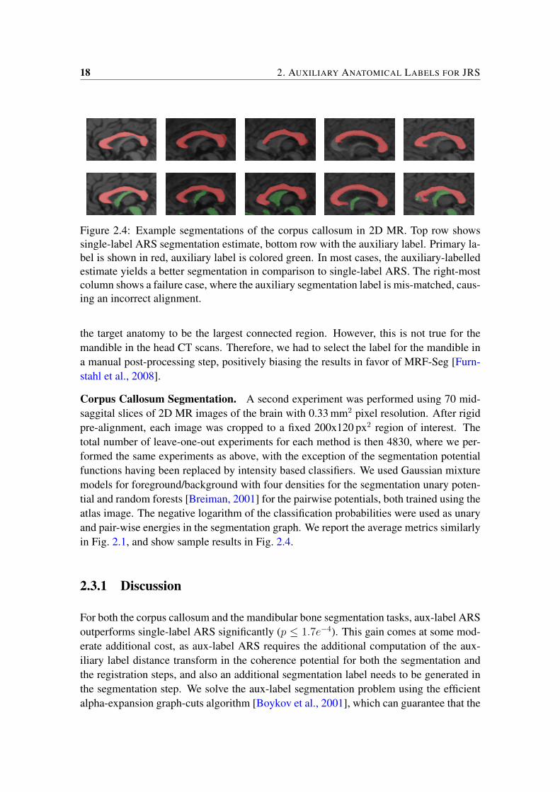
Figure 2.4: Example segmentations of the corpus callosum in 2D MR. Top row showssingle-label ARS segmentation estimate, bottom row with the auxiliary label. Primary la-bel is shown in red, auxiliary label is colored green. In most cases, the auxiliary-labelledestimate yields a better segmentation in comparison to single-label ARS. The right-mostcolumn shows a failure case, where the auxiliary segmentation label is mis-matched, caus-ing an incorrect alignment.
the target anatomy to be the largest connected region. However, this is not true for themandible in the head CT scans. Therefore, we had to select the label for the mandible ina manual post-processing step, positively biasing the results in favor of MRF-Seg [Furn-stahl et al., 2008].
Corpus Callosum Segmentation. A second experiment was performed using 70 mid-saggital slices of 2D MR images of the brain with 0.33 mm2 pixel resolution. After rigidpre-alignment, each image was cropped to a fixed 200x120 px2 region of interest. Thetotal number of leave-one-out experiments for each method is then 4830, where we per-formed the same experiments as above, with the exception of the segmentation potentialfunctions having been replaced by intensity based classifiers. We used Gaussian mixturemodels for foreground/background with four densities for the segmentation unary poten-tial and random forests [Breiman, 2001] for the pairwise potentials, both trained using theatlas image. The negative logarithm of the classification probabilities were used as unaryand pair-wise energies in the segmentation graph. We report the average metrics similarlyin Fig. 2.1, and show sample results in Fig. 2.4.
2.3.1 Discussion
For both the corpus callosum and the mandibular bone segmentation tasks, aux-label ARSoutperforms single-label ARS significantly (p ≤ 1.7e−4). This gain comes at some mod-erate additional cost, as aux-label ARS requires the additional computation of the aux-iliary label distance transform in the coherence potential for both the segmentation andthe registration steps, and also an additional segmentation label needs to be generated inthe segmentation step. We solve the aux-label segmentation problem using the efficientalpha-expansion graph-cuts algorithm [Boykov et al., 2001], which can guarantee that the
2.4. CONCLUSIONS 19
0.65
0.7
0.75
0.8
0.85
0.9
0.95
0.01 0.1 1 10 100 1000 10000
2
4
6
8
10
12
14S
eg
me
nta
tio
n o
ve
rla
p [
Dic
e]
Ha
usd
orf
f d
ista
nce
[m
m]
coherence weight
single label [Dice]single label [HD]
aux-label [Dice]aux-label [HD]
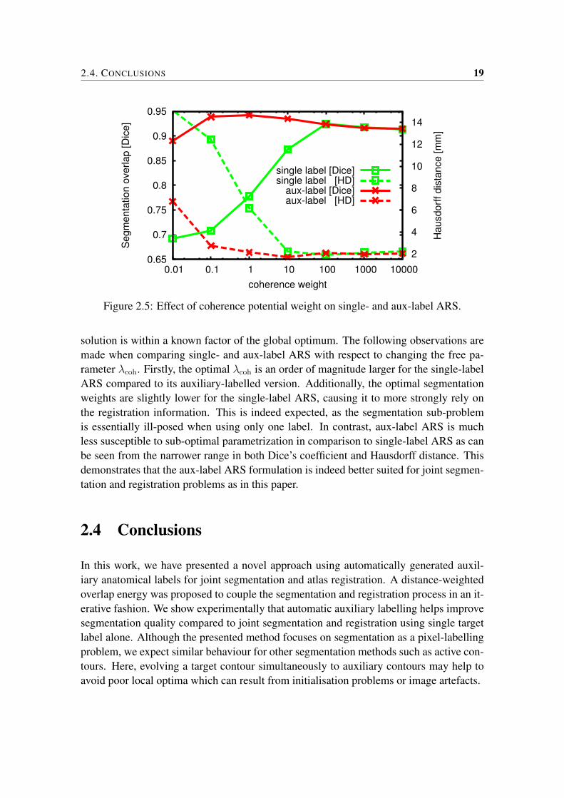
Figure 2.5: Effect of coherence potential weight on single- and aux-label ARS.
solution is within a known factor of the global optimum. The following observations aremade when comparing single- and aux-label ARS with respect to changing the free pa-rameter λcoh. Firstly, the optimal λcoh is an order of magnitude larger for the single-labelARS compared to its auxiliary-labelled version. Additionally, the optimal segmentationweights are slightly lower for the single-label ARS, causing it to more strongly rely onthe registration information. This is indeed expected, as the segmentation sub-problemis essentially ill-posed when using only one label. In contrast, aux-label ARS is muchless susceptible to sub-optimal parametrization in comparison to single-label ARS as canbe seen from the narrower range in both Dice’s coefficient and Hausdorff distance. Thisdemonstrates that the aux-label ARS formulation is indeed better suited for joint segmen-tation and registration problems as in this paper.
2.4 Conclusions
In this work, we have presented a novel approach using automatically generated auxil-iary anatomical labels for joint segmentation and atlas registration. A distance-weightedoverlap energy was proposed to couple the segmentation and registration process in an it-erative fashion. We show experimentally that automatic auxiliary labelling helps improvesegmentation quality compared to joint segmentation and registration using single targetlabel alone. Although the presented method focuses on segmentation as a pixel-labellingproblem, we expect similar behaviour for other segmentation methods such as active con-tours. Here, evolving a target contour simultaneously to auxiliary contours may help toavoid poor local optima which can result from initialisation problems or image artefacts.

3Simultaneous Segmentation andMulti-Resolution Nonrigid AtlasRegistration
In this paper, a novel Markov random field (MRF) based approach is presented for seg-menting medical images while simultaneously registering an atlas non-rigidly. In the liter-ature, both segmentation and registration have been studied extensively. For applicationsthat involve both, such as segmentation via atlas-based registration, earlier studies pro-posed addressing these problems iteratively by feeding the output of each to initialize theother. This scheme, however, cannot guarantee an optimal solution for the combined taskat hand, since these two individual problems are then treated separately. In this paper, weformulate simultaneous registration and segmentation (SRS) as a maximum a-posteriori(MAP) problem. We decompose the resulting probabilities such that the MAP inferencecan be done using MRFs. An efficient hierarchical implementation is employed, allowingcoarse-to-fine registration while estimating segmentation at pixel level. The method isevaluated on two clinical datasets: mandibular bone segmentation in 3D CT and corpuscallosum segmentation in 2D mid-saggital slices of brain MRI. A video tracking exampleis also given. Our implementation allows us to directly compare the proposed methodwith the individual segmentation/registration and the iterative approach using the exactsame potential functions. In a leave-one-out evaluation, SRS demonstrated more accurateresults in terms of Dice overlap and surface distance metrics for both datasets. We alsoshow quantitatively that the SRS method is less sensitive to the errors in the registrationas opposed to the iterative approach.
This chapter has been published as: Gass, T., Szekely, G., and Goksel, O. (2014e). SimultaneousSegmentation and Multi-Resolution Nonrigid Atlas Registration. IEEE Transactions on Image Processing,23(7):2931–2943
22 3. SIMULTANEOUS SEGMENTATION AND ATLAS REGISTRATION
Input Reg. Seg. SRS
A SA X T reg(A) T reg(SA) SsegX T srs(A) T srs(SA) Ssrs
X
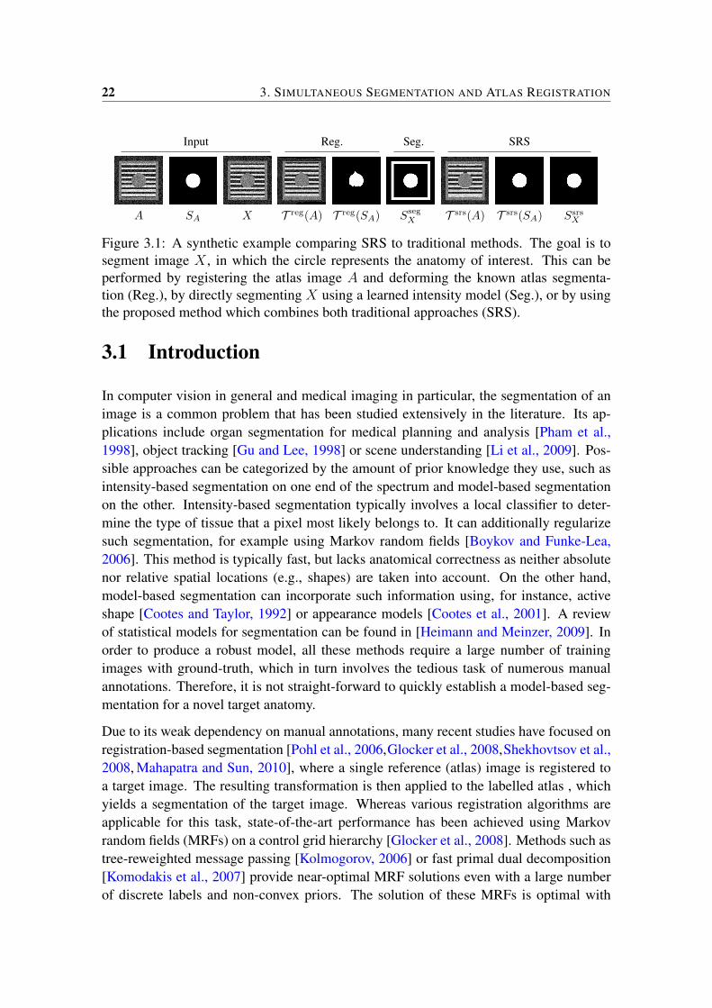
Figure 3.1: A synthetic example comparing SRS to traditional methods. The goal is tosegment image X , in which the circle represents the anatomy of interest. This can beperformed by registering the atlas image A and deforming the known atlas segmenta-tion (Reg.), by directly segmenting X using a learned intensity model (Seg.), or by usingthe proposed method which combines both traditional approaches (SRS).
3.1 Introduction
In computer vision in general and medical imaging in particular, the segmentation of animage is a common problem that has been studied extensively in the literature. Its ap-plications include organ segmentation for medical planning and analysis [Pham et al.,1998], object tracking [Gu and Lee, 1998] or scene understanding [Li et al., 2009]. Pos-sible approaches can be categorized by the amount of prior knowledge they use, such asintensity-based segmentation on one end of the spectrum and model-based segmentationon the other. Intensity-based segmentation typically involves a local classifier to deter-mine the type of tissue that a pixel most likely belongs to. It can additionally regularizesuch segmentation, for example using Markov random fields [Boykov and Funke-Lea,2006]. This method is typically fast, but lacks anatomical correctness as neither absolutenor relative spatial locations (e.g., shapes) are taken into account. On the other hand,model-based segmentation can incorporate such information using, for instance, activeshape [Cootes and Taylor, 1992] or appearance models [Cootes et al., 2001]. A reviewof statistical models for segmentation can be found in [Heimann and Meinzer, 2009]. Inorder to produce a robust model, all these methods require a large number of trainingimages with ground-truth, which in turn involves the tedious task of numerous manualannotations. Therefore, it is not straight-forward to quickly establish a model-based seg-mentation for a novel target anatomy.
Due to its weak dependency on manual annotations, many recent studies have focused onregistration-based segmentation [Pohl et al., 2006,Glocker et al., 2008,Shekhovtsov et al.,2008, Mahapatra and Sun, 2010], where a single reference (atlas) image is registered toa target image. The resulting transformation is then applied to the labelled atlas , whichyields a segmentation of the target image. Whereas various registration algorithms areapplicable for this task, state-of-the-art performance has been achieved using Markovrandom fields (MRFs) on a control grid hierarchy [Glocker et al., 2008]. Methods such astree-reweighted message passing [Kolmogorov, 2006] or fast primal dual decomposition[Komodakis et al., 2007] provide near-optimal MRF solutions even with a large numberof discrete labels and non-convex priors. The solution of these MRFs is optimal with
3.1. INTRODUCTION 23
(a) Multi-res. reg. (b) Pixel-level seg.
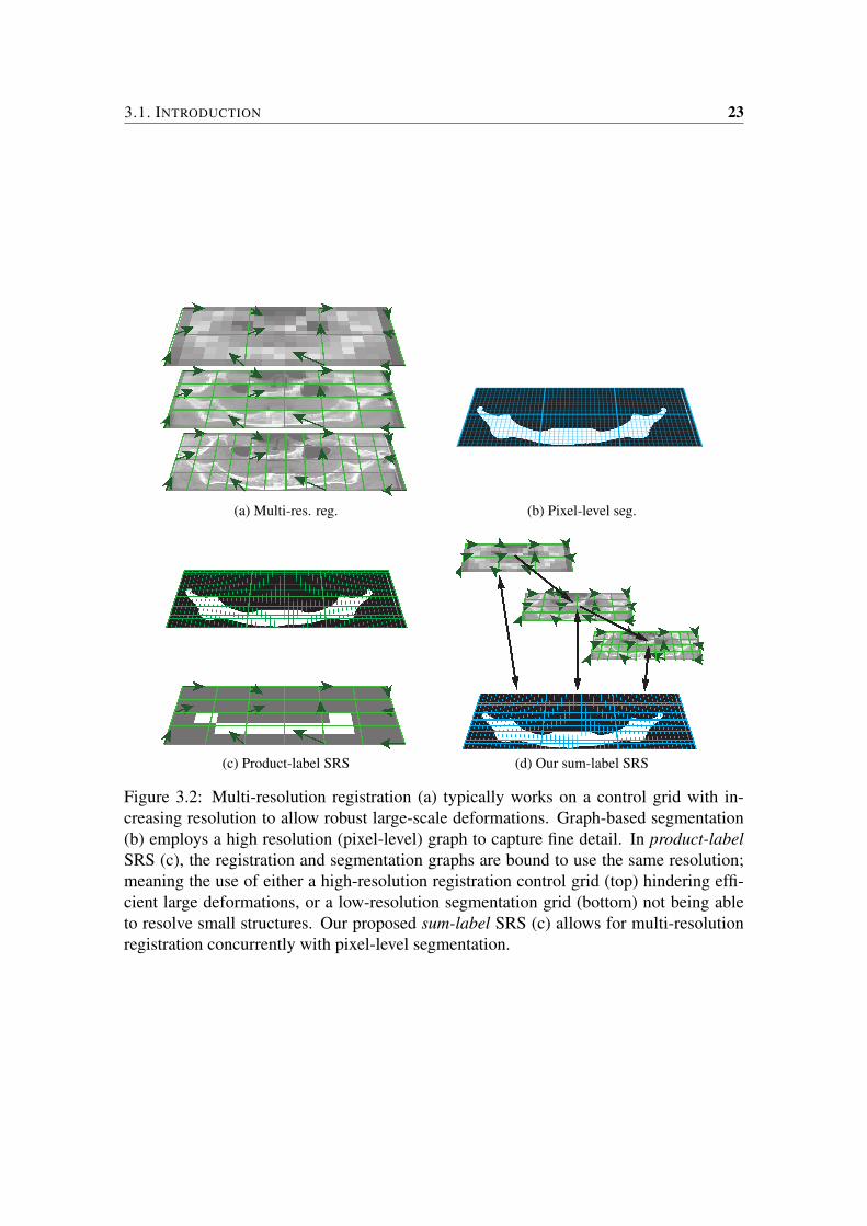
(c) Product-label SRS (d) Our sum-label SRS
Figure 3.2: Multi-resolution registration (a) typically works on a control grid with in-creasing resolution to allow robust large-scale deformations. Graph-based segmentation(b) employs a high resolution (pixel-level) graph to capture fine detail. In product-labelSRS (c), the registration and segmentation graphs are bound to use the same resolution;meaning the use of either a high-resolution registration control grid (top) hindering effi-cient large deformations, or a low-resolution segmentation grid (bottom) not being ableto resolve small structures. Our proposed sum-label SRS (c) allows for multi-resolutionregistration concurrently with pixel-level segmentation.
24 3. SIMULTANEOUS SEGMENTATION AND ATLAS REGISTRATION
respect to a selected criterion, often defined as a global similarity metric to reduce thedifference between the target image and the deformed atlas image. While being widelyused in medical imaging, image registration alone cannot solve the segmentation task byitself as it is considered to be an ill-posed problem [Fischer and Modersitzki, 2008]. Thisis because anatomical correspondences, which are not guaranteed to exist, are computedusing surrogate criteria such as intensity similarity. In addition, the problem of non-rigid registration is known to be NP-complete [Keysers and Unger, 2003], thus makingapproximative algorithms prone to local optima, for example due to poor initialization.Increasing the amount of prior knowledge is a common remedy for such problems, forexample by including statistical or multiple atlases [Rohlfing et al., 2005, Heckemannet al., 2006, Glocker et al., 2007].
Joint optimization of the segmentation and registration was first proposed by [Wyatt andNoble, 2003]. In alternating registration and segmentation(ARS), the estimated solu-tion for one subproblem is used as prior knowledge in the other in an iterative manner,whereas simultaneous registration and segmentation(SRS) aims at optimizing both goalsat the same time. A comparison of individual and joint approaches is demonstrated on asynthetic example in Fig. 3.1. To the best of our knowledge, almost all approaches pub-lished so far in the field have followed the ARS approach; the wording “simultaneous”was used commonly, though it was not used per se as defined above. The method pro-posed in [Wyatt and Noble, 2003] alternates between estimating a rigid transformationusing Powells’ method and updating the segmentation using iterative conditional modes(ICM) in an MRF. [Pohl et al., 2006] proposed a Bayesian framework in which they al-ternate between updating the registration and estimating intensity “nuisance” parameterswhile marginalizing over possible anatomical labels using an EM algorithm. [Xiaohuaet al., 2004] proposed an ARS approach based on MRFs. Their method alternates be-tween solving one MRF that optimizes registration parameters and updates segmentationprobabilities, and a second MRF solving the segmentation. There have been also stud-ies on alternating registration and segmentation in variational formulations, which alsorely on iteratively updating the registration and segmentation solutions, for example, byusing gradient descent [Wang et al., 2006a, Ghosh et al., 2010, Schmidt-Richberg andEhrhardt, 2012]. For example, a method which alternates between updating the deforma-tion field using a quasi-Newton optimization method and evolving a contour in the targetimage while constraining the distance between deformed atlas and said target contour wasproposed in [Wang et al., 2006a]. It is also possible to combine registration with model-based segmentation as shown in [Lu and Duncan, 2012], where point-based registrationand active-shape segmentation trained from manually annotated images are employed formutual benefit.
For non-medical applications, optical flow [Horn and Schunck, 1981] has been frequentlyused for estimating the motion in image sequences or stereo images. Such inter-frameflow estimations may though fail in the presence of occlusions – a problem indeed similarto its medical image registration counterpart when posed as a lack of complete correspon-
3.1. INTRODUCTION 25
dences between frames. To alleviate this, several studies focused on estimating opticalflow while jointly computing a segmentation. For example, [Sudderth and Black, 2012]segments an image sequence into layers while estimating flow. Information from sucha sequence then helps resolve occlusions. A different technique was presented in [Leiand Yang, 2009], where optical flow is computed on a hierarchy of over-segmentationsbased on super-pixels. Note that such techniques do not operate on 3D images. Further-more, they are not designed to accommodate large deformations expected in inter-patientregistration. Therefore, those methods are not applicable in our targeted domain.
For simultaneous registration and image based segmentation, Markov random field basedapproaches are attractive due to the following reasons: (i) Image segmentation is naturallya discrete labelling problem, for which MRFs can efficiently find excellent solutions. (ii)Registration can also be defined as a discrete optimization problem [Glocker et al., 2008],which does not rely on gradients and is thus potentially less sensitive to local minima, forexample, due to poor initialisation. Two recent methods in the literature have exploredsuch MRF-based simultaneous segmentation and registration: In [Mahapatra and Sun,2012], intra-patient time-series image registration was shown to be improved by simulta-neously estimating a segmentation of target and floating image using a user-defined ROI.This work does not use an atlas segmentation and targets only small displacements, whichwill prevent inter-patient registration. In [Parisot et al., 2012], a healthy brain was regis-tered to one with a tumor while the tumor in the target was being segmented. This methodinfers tumor tissue from registration non-overlap (tear), and vice versa. Note that, simi-larly to [Mahapatra and Sun, 2012], this work does not use an atlas segmentation either,as the healthy atlas does not contain a tumor.
Compared to other SRS approaches in the literature, we target inter-patient atlas-basedsegmentation. Indeed, our SRS technique was developed to address several aspects re-quired for this task, for which other existing approaches are not suitable. The biggestdifference of our SRS technique from other approaches is our design to accommodatedifferent levels of detail for the segmentation and registration subproblems concurrently.Without allowing for different levels of detail, an SRS solution will either be unable torobustly model large deformations (e.g., in [Mahapatra and Sun, 2012]) inevitable in inter-atlas registrations; or will lead to very coarse segmentations (e.g., in [Parisot et al., 2012])unusable for precise delineation. Our method not only can handle both of those at thesame time, but it also can do this without increasing the computational cost significantly,due to the treatment of the solution label-space. To clarify such difference, we name thepreviously proposed techniques product-label SRS, as they search for a discrete labellingin the product label space of segmentation and registration labels. Our method can incontrast be called sum-label SRS, as its solution label space is the union of segmentationand registration label spaces and therefore the total number of labels is the sum of thenumber of registration and segmentation labels. This fundamental difference is illustratedon MRF-graphs in Fig. 3.2. Different levels of detail are accommodated in this paper byour novel two-layer graph structure connected by inter-layer edges that model a coher-

26 3. SIMULTANEOUS SEGMENTATION AND ATLAS REGISTRATION
ence potential. Thanks to our elaborate probabilistic derivation of the underlying SRSproblem, we could then soundly define each component of such a two-layer model by asuitable energy term.
Accordingly, the contributions of this paper can be listed as follows: (i.) Our novel si-multaneous registration and segmentation method allows pixel-level segmentation withsimultaneous multi-level non-rigid registration. (ii.) In contrast to previous SRS-like ap-proaches, our work utilizes a known atlas segmentation. (iii.) Our SRS model is deriventhrough a rigorous Bayesian analysis of the underlying maximum a posteriori problem.(iv.) Experimental comparison between alternating and simultaneous segmentation andregistration approaches is presented within the same framework.
This paper is structured as follows. First, we introduce the general concepts and ournotation. Next, our decomposition of the underlying MAP criterion is presented. Then,the structure of the resulting MRF is given, followed by our implementation. The paperis concluded with an experimental evaluation on two clinical datasets.
3.2 Background and Notation
Let X be the target and A the atlas image, where both are functions Ω → F . Ω ∈ND is the D-dimensional discretized coordinate domain, and F is an arbitrary featuredescriptor, e.g. the image intensity in many cases or a feature vector. A segmentationS = lS0 , · · · , lSN is an assignement of one segmentation label lS out of the set of allsegmentation labels LS to each of the N pixels of an image. In a plain segmentation task,the segmentation SX of the target image X is sought. In contrast, in a plain registrationtask the goal is to find a transformation T such that the target imageX and the transformedatlas image A(T ) become similar according to an appropriately selected measure. In ourcase, T is a non-rigid deformation represented by a D-dimensional displacement vectorfield T : Ω→ RD so that for each pixel/voxel i ∈ Ω:
T (i) = i+ Ti. (3.1)
Ti and Ti are short-hands for the local deformation T (i) and displacement T (i). Wewill also use this notation to denote pixels in an image I as Ii, e.g. Xi, Ai. I(T ) = i →I(i+ Ti) ∀i, indicates a deformed image. Values at non-grid locations are interpolated.
Both finding a displacement vector field T and finding a segmentation SX can be definedas separate maximum a-posteriori (MAP) problems as follows:
SX = arg maxSX
p(SX |X) (3.2)
T = arg maxT
p(T |X,A) (3.3)
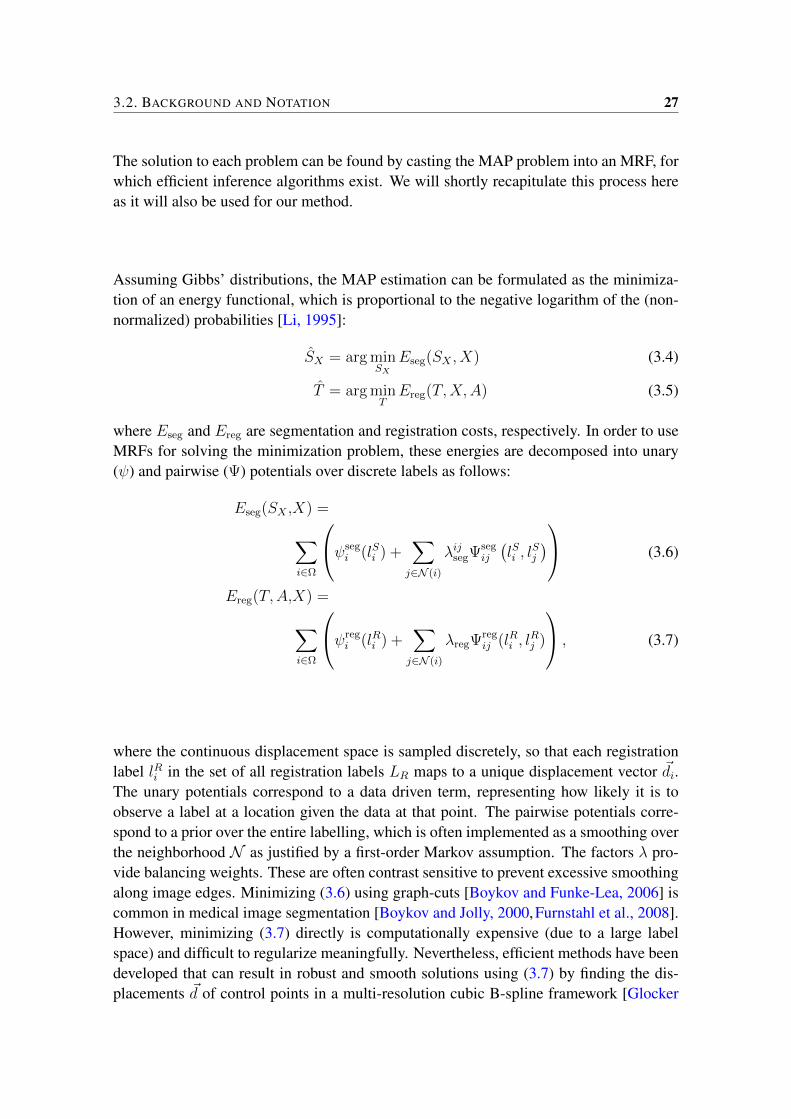
3.2. BACKGROUND AND NOTATION 27
The solution to each problem can be found by casting the MAP problem into an MRF, forwhich efficient inference algorithms exist. We will shortly recapitulate this process hereas it will also be used for our method.
Assuming Gibbs’ distributions, the MAP estimation can be formulated as the minimiza-tion of an energy functional, which is proportional to the negative logarithm of the (non-normalized) probabilities [Li, 1995]:
SX = arg minSX
Eseg(SX , X) (3.4)
T = arg minTEreg(T,X,A) (3.5)
where Eseg and Ereg are segmentation and registration costs, respectively. In order to useMRFs for solving the minimization problem, these energies are decomposed into unary(ψ) and pairwise (Ψ) potentials over discrete labels as follows:
Eseg(SX ,X) =∑i∈Ω
ψsegi (lSi ) +
∑j∈N (i)
λijsegΨsegij
(lSi , l
Sj
) (3.6)
Ereg(T,A,X) =∑i∈Ω
ψregi (lRi ) +
∑j∈N (i)
λregΨregij (lRi , l
Rj )
, (3.7)
where the continuous displacement space is sampled discretely, so that each registrationlabel lRi in the set of all registration labels LR maps to a unique displacement vector ~di.The unary potentials correspond to a data driven term, representing how likely it is toobserve a label at a location given the data at that point. The pairwise potentials corre-spond to a prior over the entire labelling, which is often implemented as a smoothing overthe neighborhood N as justified by a first-order Markov assumption. The factors λ pro-vide balancing weights. These are often contrast sensitive to prevent excessive smoothingalong image edges. Minimizing (3.6) using graph-cuts [Boykov and Funke-Lea, 2006] iscommon in medical image segmentation [Boykov and Jolly, 2000,Furnstahl et al., 2008].However, minimizing (3.7) directly is computationally expensive (due to a large labelspace) and difficult to regularize meaningfully. Nevertheless, efficient methods have beendeveloped that can result in robust and smooth solutions using (3.7) by finding the dis-placements ~d of control points in a multi-resolution cubic B-spline framework [Glocker

28 3. SIMULTANEOUS SEGMENTATION AND ATLAS REGISTRATION
et al., 2008]. Such control points are placed on a coarse Cartesian grid, which allowscomputing the displacement at a position ~x = (x, y) as follows:
T (~x) =3∑l=0
3∑m=0
Bl(u)Bm(v)~di+l,j+m, (3.8)
where i and j are the indices of the closest grid control point to ~x; u and v are the nor-malized distances to this control point; and Bl is the lth B-spline basis function. Thethree-dimensional interpolation can be defined analogously.
Given the atlas segmentation SA, one iteration of the alternating approach ARS can beformulated similarly to [Wyatt and Noble, 2003] as:
T n+1 = arg maxT
p(T |X,A, SA, SnX) (3.9)
Sn+1X = arg max
SX
p(SX |X,A, SA, T n+1). (3.10)
where T 0 is initialized using plain (often intensity-based) registration and the optimizationis terminated upon convergence of these terms. Note that here each maximization problemcan be solved using MRFs, iterative methods or a combination thereof, as investigated indifferent studies in the literature.
3.3 Simultaneous Registration and Segmentation
In simultaneous registration and segmentation (SRS), one seeks for the segmentation SXand the displacement field T that maximize the joint posterior probability given the targetand atlas image and the atlas segmentation:
(SX , T ) = arg maxSX ,T
p(SX , T |X,A, SA). (3.11)
As this posterior distribution is not trivial to model, let alone devise an algorithm to findthe MAP solution, we first decompose this full problem within the Bayesian framework
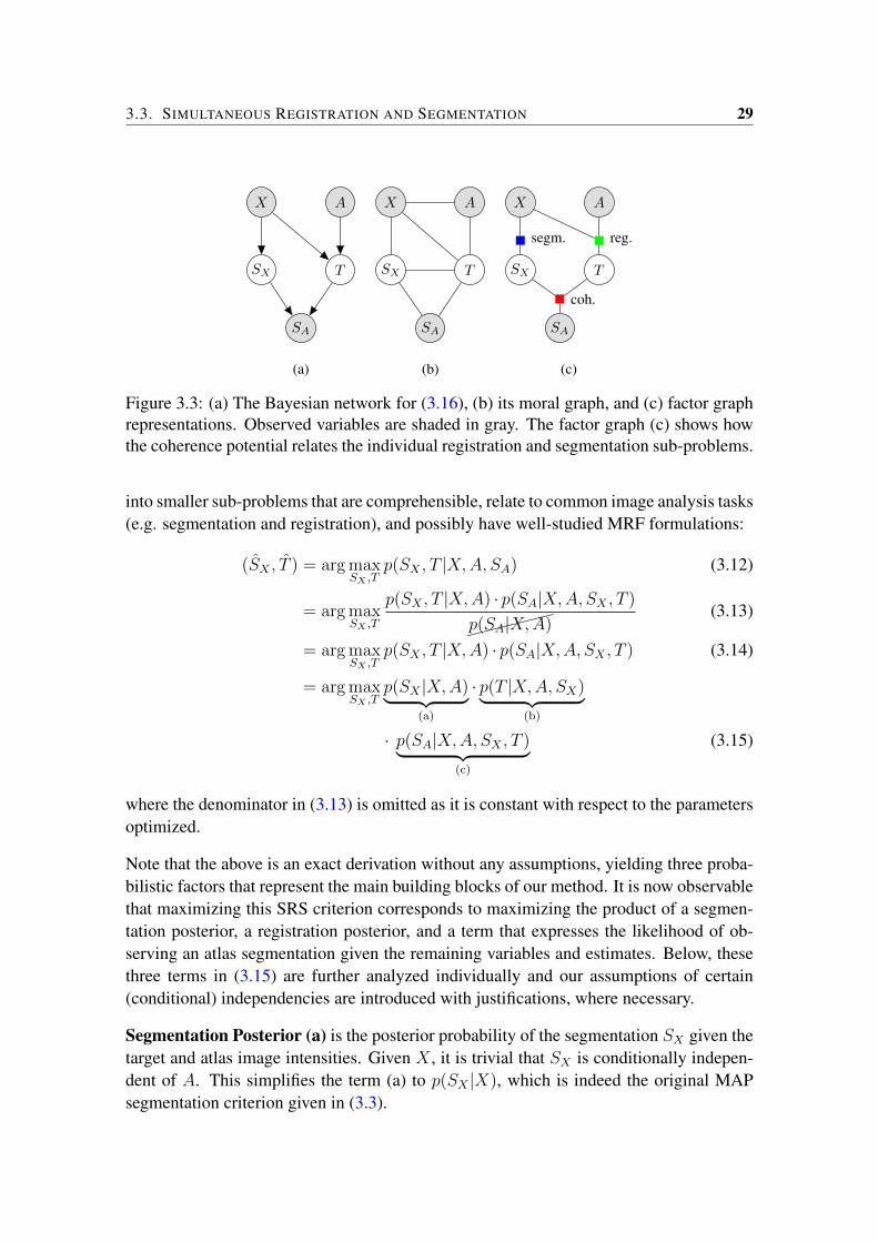
3.3. SIMULTANEOUS REGISTRATION AND SEGMENTATION 29
X A
SX T
SA
(a)
X A
SX T
SA
(b)
X A
SX T
SA
segm. reg.
coh.
(c)
Figure 3.3: (a) The Bayesian network for (3.16), (b) its moral graph, and (c) factor graphrepresentations. Observed variables are shaded in gray. The factor graph (c) shows howthe coherence potential relates the individual registration and segmentation sub-problems.
into smaller sub-problems that are comprehensible, relate to common image analysis tasks(e.g. segmentation and registration), and possibly have well-studied MRF formulations:
(SX , T ) = arg maxSX ,T
p(SX , T |X,A, SA) (3.12)
= arg maxSX ,T
p(SX , T |X,A) · p(SA|X,A, SX , T )
p(SA|X,A)
(3.13)
= arg maxSX ,T
p(SX , T |X,A) · p(SA|X,A, SX , T ) (3.14)
= arg maxSX ,T
p(SX |X,A)︸ ︷︷ ︸(a)
· p(T |X,A, SX)︸ ︷︷ ︸(b)
· p(SA|X,A, SX , T )︸ ︷︷ ︸(c)
(3.15)
where the denominator in (3.13) is omitted as it is constant with respect to the parametersoptimized.
Note that the above is an exact derivation without any assumptions, yielding three proba-bilistic factors that represent the main building blocks of our method. It is now observablethat maximizing this SRS criterion corresponds to maximizing the product of a segmen-tation posterior, a registration posterior, and a term that expresses the likelihood of ob-serving an atlas segmentation given the remaining variables and estimates. Below, thesethree terms in (3.15) are further analyzed individually and our assumptions of certain(conditional) independencies are introduced with justifications, where necessary.
Segmentation Posterior (a) is the posterior probability of the segmentation SX given thetarget and atlas image intensities. Given X , it is trivial that SX is conditionally indepen-dent of A. This simplifies the term (a) to p(SX |X), which is indeed the original MAPsegmentation criterion given in (3.3).

30 3. SIMULTANEOUS SEGMENTATION AND ATLAS REGISTRATION
Registration Posterior (b) is the posterior probability of the deformation T given thetarget and atlas intensities, as well as the target segmentation SX . Here, we introduce theassumption that T is independent of SX , givenA andX . Note that this effectively restrictsthe use of smoothing the deformation differently at object boundaries defined by SX .Nevertheless, such smoothing is already not feasible at coarse levels of deformation weemploy. The final term is then identical to the MAP criterion given for image registrationin (3.3).
Coherence (c) is the probability of observing SA, given SX , T,X,A. This term thuscontrols the similarity of the (deformed) atlas segmentation and the target segmentationestimates. It can be simplified by assuming that SA is independent of X,A, given SXand T . It is important to note that this term motivates the modelling of uncertainty in theSRS process, since it expresses a probabilistic relation between SX and SA(T ) rather thanassuming SX = SA(T ).
The observations above then lead to the following final MAP formulation for simultane-ous segmentation and registration:
(SX , T ) = arg maxSX ,T
p(SX |X)︸ ︷︷ ︸segmentation
p(T |A,X)︸ ︷︷ ︸registration
p(SA|SX , T )︸ ︷︷ ︸coherence
, (3.16)
where the segmentation SX and the registration T are connected (indirectly) through thecoherence factor p(SA|SX , T ). This is visualized formally in Fig. 3.3, where the Bayesiannetwork defined by (3.16) and its conversion to a factor graph are shown. This definitionhas the advantage that both the registration and the segmentation appear in a common,well-studied form and thus both can be estimated using well-known, state-of-the-art tech-niques. In addition, the coherence term can be implemented efficiently as we will showbelow .
3.4 Implementation using Markov Random Fields
In order to solve the MAP problem, we cast it into an MRF, for which efficient inferencealgorithms exist. We will first motivate and describe the structure of the MRF beforedetailing the implementation of the potential functions and its optimization.
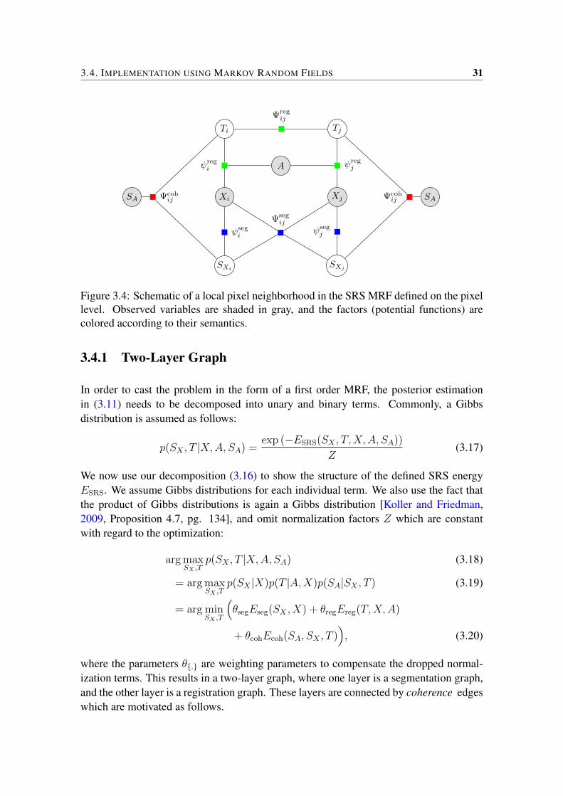
3.4. IMPLEMENTATION USING MARKOV RANDOM FIELDS 31
Ti Tj
A
SA Xi Xj SA
SXiSXj
Ψregij
ψregi ψreg
j
ψsegi
ψsegj
Ψsegij
Ψcohij Ψcoh
ij
Figure 3.4: Schematic of a local pixel neighborhood in the SRS MRF defined on the pixellevel. Observed variables are shaded in gray, and the factors (potential functions) arecolored according to their semantics.
3.4.1 Two-Layer Graph
In order to cast the problem in the form of a first order MRF, the posterior estimationin (3.11) needs to be decomposed into unary and binary terms. Commonly, a Gibbsdistribution is assumed as follows:
p(SX , T |X,A, SA) =exp (−ESRS(SX , T,X,A, SA))
Z(3.17)
We now use our decomposition (3.16) to show the structure of the defined SRS energyESRS. We assume Gibbs distributions for each individual term. We also use the fact thatthe product of Gibbs distributions is again a Gibbs distribution [Koller and Friedman,2009, Proposition 4.7, pg. 134], and omit normalization factors Z which are constantwith regard to the optimization:
arg maxSX ,T
p(SX , T |X,A, SA) (3.18)
= arg maxSX ,T
p(SX |X)p(T |A,X)p(SA|SX , T ) (3.19)
= arg minSX ,T
(θsegEseg(SX , X) + θregEreg(T,X,A)
+ θcohEcoh(SA, SX , T )), (3.20)
where the parameters θ. are weighting parameters to compensate the dropped normal-ization terms. This results in a two-layer graph, where one layer is a segmentation graph,and the other layer is a registration graph. These layers are connected by coherence edgeswhich are motivated as follows.
32 3. SIMULTANEOUS SEGMENTATION AND ATLAS REGISTRATION
The coherence potential couples the registration and segmentation potential by introduc-ing the likelihood of observing an atlas segmentation given registration and target seg-mentation estimates. Intuitively, it shall yield a high probability, when the deformed atlassegmentation SA(T ) can be well explained by the target segmentation SX . The likeli-hoods can be computed locally analogously to the unary potentials in (3.6) and (3.7).Then, the coherence term in (3.16) can be rewritten as:
p(SA|SX , T ) = p(SA(T )|SX) (3.21)
=∏i∈Ω
pi(SA(Ti)|lSi ) . (3.22)
This allows modelling the coherence for each pixel individually, and to convert it into anenergy similar to (3.6):
Ecoh(SA, T, SX) =∑i∈Ω
Ψcohij (lRi , l
Si ), (3.23)
where Ψcohij ∝ − log(pi(SA(Ti)|lSi )) is a pairwise potential function over the joint label
space of the segmentation and registration labels which will be defined in Sec. 3.4.3.This definition of the coherence potentials along with the segmentation and registrationenergies defined in (3.6,3.7) entails an MRF on the pixel level which is shown in Fig. 3.4.As mentioned earlier, this will make the method either computationally expensive or limitthe possible range of deformations. We thus propose the following novel multi-resolutionframework for SRS.
3.4.2 SRS using a Multi-Resolution Framework
Despite a coarse-to-fine approach for registration and different grid resolutions/iterationsthereby employed, we perform segmentation at a fine level at all times. Accordingly, thesegmentation energy Eseg is implemented as given in (3.6) at pixel resolution similarlyto conventional MRF-based segmentation methods. For the registration, however, we usea multi-resolution registration approach [Glocker et al., 2008], where only the displace-ments of a coarse (Cartesian) control grid are estimated iteratively. Similarly to [Glockeret al., 2008], such grid displacements are applied to the full-resolution image at each itera-tion using B-spline transform as in (3.8). Then, the Ereg in MRF can be defined similarlyto (3.7), but now on a graph Greg with nodes representing grid corner displacements asfollows:
Ereg(T,A,X) =∑i∈Greg
(ψregi (lRi ) +
∑j∈N (i)
Ψregij (lRi , l
Rj )
)(3.24)
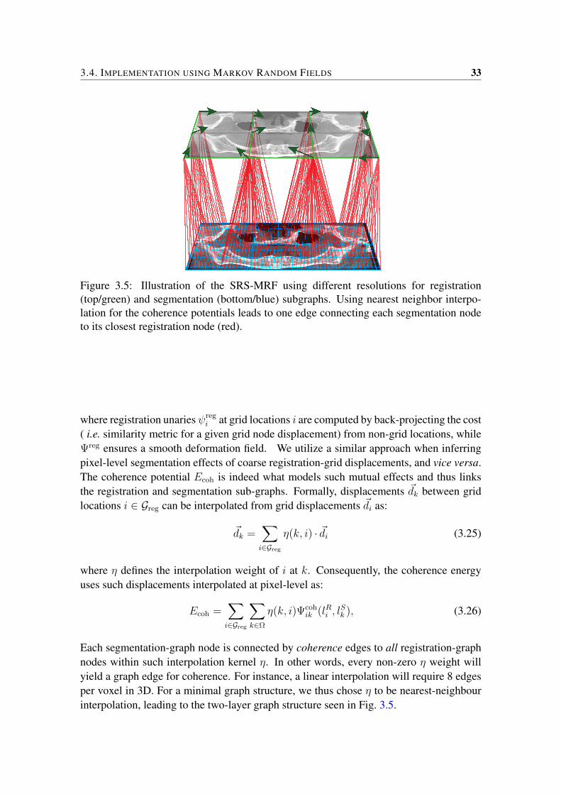
3.4. IMPLEMENTATION USING MARKOV RANDOM FIELDS 33
Figure 3.5: Illustration of the SRS-MRF using different resolutions for registration(top/green) and segmentation (bottom/blue) subgraphs. Using nearest neighbor interpo-lation for the coherence potentials leads to one edge connecting each segmentation nodeto its closest registration node (red).
where registration unariesψregi at grid locations i are computed by back-projecting the cost
( i.e. similarity metric for a given grid node displacement) from non-grid locations, whileΨreg ensures a smooth deformation field. We utilize a similar approach when inferringpixel-level segmentation effects of coarse registration-grid displacements, and vice versa.The coherence potential Ecoh is indeed what models such mutual effects and thus linksthe registration and segmentation sub-graphs. Formally, displacements ~dk between gridlocations i ∈ Greg can be interpolated from grid displacements ~di as:
~dk =∑i∈Greg
η(k, i) · ~di (3.25)
where η defines the interpolation weight of i at k. Consequently, the coherence energyuses such displacements interpolated at pixel-level as:
Ecoh =∑i∈Greg
∑k∈Ω
η(k, i)Ψcohik (lRi , l
Sk ), (3.26)
Each segmentation-graph node is connected by coherence edges to all registration-graphnodes within such interpolation kernel η. In other words, every non-zero η weight willyield a graph edge for coherence. For instance, a linear interpolation will require 8 edgesper voxel in 3D. For a minimal graph structure, we thus chose η to be nearest-neighbourinterpolation, leading to the two-layer graph structure seen in Fig. 3.5.
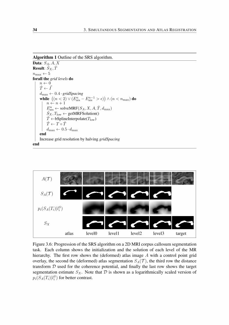
34 3. SIMULTANEOUS SEGMENTATION AND ATLAS REGISTRATION
Algorithm 1 Outline of the SRS algorithm.Data: SA, A,XResult: SX , Tnmax ← 5forall the grid levels do
n← 0T ← ~Idmax ← 0.4 · gridSpacingwhile
((n < 2) ∨ (Ensrs − En−1
srs > ε))∧ (n < nmax) do
n← n+ 1Ensrs ← solveMRF(SA, X,A, T , dmax)SX , Tlow ← getMRFSolution()T ←bSplineInterpolate(Tlow)T ← T Tdmax ← 0.5 · dmax
endIncrease grid resolution by halving gridSpacing
end
A(T )
SA(T )
pi(SA(Ti)|lSi )
SX
atlas level0 level1 level2 level3 target
Figure 3.6: Progression of the SRS algorithm on a 2D MRI corpus callosum segmentationtask. Each column shows the initialization and the solution of each level of the MRhierarchy. The first row shows the (deformed) atlas image A with a control point gridoverlay, the second the (deformed) atlas segmentation SA(T ), the third row the distancetransform D used for the coherence potential, and finally the last row shows the targetsegmentation estimate SX . Note that D is shown as a logarithmically scaled version ofpi(SA(Ti)|lSi ) for better contrast.
3.4. IMPLEMENTATION USING MARKOV RANDOM FIELDS 35
3.4.3 Algorithm
Having defined the MRF structure above, we now summarize our algorithm next. As amulti-resolution approach, it solves a sequence of individual MRFs with different regis-tration control grid resolutions. The deformations from each step are then composed toinitialize the next step. This process is outlined in Alg. 1.
We start with a coarse displacement control grid and interpolate the costs of labellingpixels at sub-grid level. We use a B-spline interpolation to interpolate the full deforma-tion once the displacements of grid control points are optimized [Szeliski and Coughlan,1997]. This interpolation is then used for the composition of the deformations at fullresolution as follows:
T = T T , T (i) = T (T (i)) + T (i). (3.27)
For efficiency reasons, we always keep the last deformation in memory at this full resolu-tion, as we would need to interpolate multiple times in the registration unary and coher-ence potentials. The coarsest control grid divides the shortest edge of the image by 3 andtries to keep square (or cubic in 3D) grid cells. This allows capturing large deformationsin registration. Similarly to [Glocker et al., 2008], the control grid resolution is doubledat each level, where the displacement parameters are optimized iteratively for each reso-lution until the convergence of the MRF energy. Such inner iterations of SRS, labelled nin Alg. 1, allows us to find precise displacements by re-sampling the displacement labelspace. The maximum sampled displacement at each inner iteration is set to be 40% ofthe control grid spacing. This guarantees that deformations are diffeomorphic when B-spline interpolating them at non-grid locations [Rueckert et al., 2006]. At each iteration,the maximum displacement dmax is then halved to increase the precision of registrationestimates (down to sub-pixel displacements) using only a limited number of displacementlabels for an efficient MRF implementation. We sample the displacements uniformly to a9 × 9 grid in 2D, while restricting the sampling to the principal axes in 3D for increasedefficiency. For the registration similarity metric, both target and atlas images are downsampled by a factor linked to the grid resolution, after smoothing with a Gaussian kernelto avoid aliasing. The kernel size of the Gaussian was set to ~σ = 0.5 ∗ (∆target−∆source),where ∆target is the target spacing, and ∆source is the spacing of the original image.
3.4.3.1 Potential Functions
In this section, we present the individual potential functions used in our approach. Wedemonstrate the flexibility of our method by using domain-specific segmentation poten-tials, which only need to satisfy general properties as imposed by the used MRF optimizer.We will explain the coherence potential in detail, while only briefly summarizing the re-maining functions as they are standard methods.
36 3. SIMULTANEOUS SEGMENTATION AND ATLAS REGISTRATION
Coherence Pairwise Ψcohij : As explained in (3.22), the coherence potential is based on
pixel-wise comparisons between the deformed atlas segmentation and the target segmen-tation estimate. We model the probability pi(SA(Ti)|lSi ) as a Gaussian based on the dis-tance of a point i and the nearest point in SA(T ) with the segmentation label lSi . LetDlSi denote the distance transform of SA with respect to label lSi . Then, we compute theprobability as:
pi(SA(Ti)|lSi
)∝ exp
(−DlSi (Ti)2
2τ 2
), (3.28)
where τ is a tolerance parameter, which we set based on multi-resolution level. Thiscan be seen in the third row of Fig. 3.6, where we started with a tolerance of 16 mmwhich is halved at every subsequent level of hierarchy. This is motivated by the fact thatthe expected difference between deformed atlas segmentation and target segmentationis larger in earlier levels compared to later stages. In experiments, a small tolerance inearly levels was observed to force the target segmentation to be grossly dissimilar to thetrue segmentation, leading to a local optimum in the iterative registration process sincethe deformed atlas segmentation has not yet aligned properly. This is mitigated by theadaptive tolerance setting proposed before. Taking the negative logarithm of (3.28), thisthen results in the following potential function:
Ψcohij (lRi , l
Si ) =
DlSi (Ti)2
2τ 2, (3.29)
We threshold the distance transforms to be≥ 0, so that the potential is zero when the labelof the deformed atlas segmentation is equal to the segmentation label, i.e. SA(Ti) = lSi .
Segmentation Unary ψsegi : Depending on the image domain, we use a different segmen-
tation potential. For CT bone images, we use a threshold-based potential using the knownHounsfield units (HU) for cortical bone (>500) and air (<-300) as presented in [Furnstahlet al., 2008]. For the brain MR images, we train a Gaussian mixture model (GMM) withtwo densities per class on the atlas (image+segmentation) and use the negative logarithmas the potential.
Segmentation Pairwise Ψsegij : Similar to the segmentation unaries, we also use domain
specific pairwise segmentation potential. For the CT images, we also use the potential of[Furnstahl et al., 2008], which is based on the contrast of a sheetness filtered version ofthe CT image [Descoteaux et al., 2006]. For the MR images, we train a random forest(RF) classifier [Breiman, 2001] using each pair of neighboring atlas image pixels as input
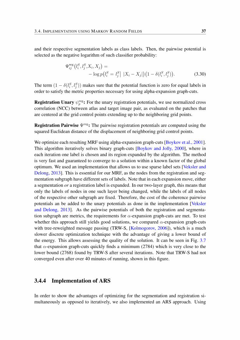
3.4. IMPLEMENTATION USING MARKOV RANDOM FIELDS 37
and their respective segmentation labels as class labels. Then, the pairwise potential isselected as the negative logarithm of such classifier probability:
Ψsegij
(lSi , l
Sj ,Xi, Xj
)=
− log p(lSi = lSj
∣∣ |Xi −Xj|)(
1− δ(lSi , lSj )). (3.30)
The term (1 − δ(lSi , lSj )) makes sure that the potential function is zero for equal labels inorder to satisfy the metric properties necessary for using alpha-expansion graph-cuts.
Registration Unary ψregp : For the unary registration potentials, we use normalized cross
correlation (NCC) between atlas and target image pair, as evaluated on the patches thatare centered at the grid control points extending up to the neighboring grid points.
Registration Pairwise Ψreg: The pairwise registration potentials are computed using thesquared Euclidean distance of the displacement of neighboring grid control points.
We optimize each resulting MRF using alpha-expansion graph-cuts [Boykov et al., 2001].This algorithm iteratively solves binary graph-cuts [Boykov and Jolly, 2000], where ineach iteration one label is chosen and its region expanded by the algorithm. The methodis very fast and guaranteed to converge to a solution within a known factor of the globaloptimum. We used an implementation that allows us to use sparse label sets [Veksler andDelong, 2013]. This is essential for our MRF, as the nodes from the registration and seg-mentation subgraph have different sets of labels. Note that in each expansion move, eithera segmentation or a registration label is expanded. In our two-layer graph, this means thatonly the labels of nodes in one such layer being changed, while the labels of all nodesof the respective other subgraph are fixed. Therefore, the cost of the coherence pairwisepotentials an be added to the unary potentials as done in the implementation [Vekslerand Delong, 2013]. As the pairwise potentials of both the registration and segmenta-tion subgraph are metrics, the requirements for α-expansion graph-cuts are met. To testwhether this approach still yields good solutions, we compared α-expansion graph-cutswith tree-reweighted message passing (TRW-S, [Kolmogorov, 2006]), which is a muchslower discrete optimization technique with the advantage of giving a lower bound ofthe energy. This allows assessing the quality of the solution. It can be seen in Fig. 3.7that α-expansion graph-cuts quickly finds a minimum (2784) which is very close to thelower bound (2768) found by TRW-S after several iterations. Note that TRW-S had notconverged even after over 40 minutes of running, shown in this figure.
3.4.4 Implementation of ARS
In order to show the advantages of optimizing for the segmentation and registration si-multaneously as opposed to iteratively, we also implemented an ARS approach. Using
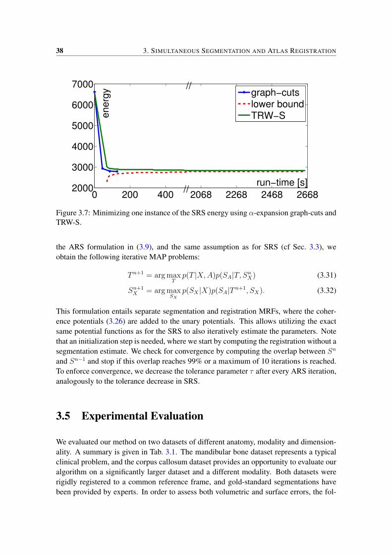
38 3. SIMULTANEOUS SEGMENTATION AND ATLAS REGISTRATION
0 200 400 2068 2268 2468 26682000
3000
4000
5000
6000
7000
run−time [s]
en
erg
y
//
//graph−cutslower boundTRW−S
Figure 3.7: Minimizing one instance of the SRS energy using α-expansion graph-cuts andTRW-S.
the ARS formulation in (3.9), and the same assumption as for SRS (cf Sec. 3.3), weobtain the following iterative MAP problems:
T n+1 = arg maxT
p(T |X,A)p(SA|T, SnX) (3.31)
Sn+1X = arg max
SX
p(SX |X)p(SA|T n+1, SX). (3.32)
This formulation entails separate segmentation and registration MRFs, where the coher-ence potentials (3.26) are added to the unary potentials. This allows utilizing the exactsame potential functions as for the SRS to also iteratively estimate the parameters. Notethat an initialization step is needed, where we start by computing the registration without asegmentation estimate. We check for convergence by computing the overlap between Sn
and Sn−1 and stop if this overlap reaches 99% or a maximum of 10 iterations is reached.To enforce convergence, we decrease the tolerance parameter τ after every ARS iteration,analogously to the tolerance decrease in SRS.
3.5 Experimental Evaluation
We evaluated our method on two datasets of different anatomy, modality and dimension-ality. A summary is given in Tab. 3.1. The mandibular bone dataset represents a typicalclinical problem, and the corpus callosum dataset provides an opportunity to evaluate ouralgorithm on a significantly larger dataset and a different modality. Both datasets wererigidly registered to a common reference frame, and gold-standard segmentations havebeen provided by experts. In order to assess both volumetric and surface errors, the fol-
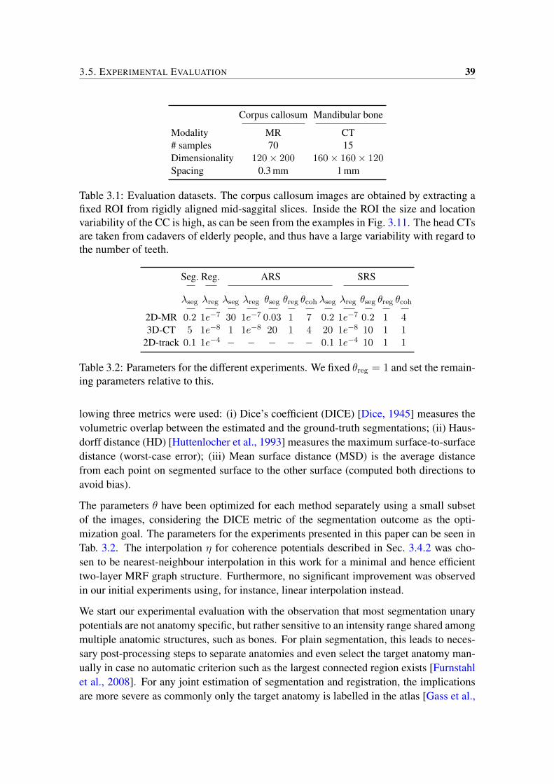
3.5. EXPERIMENTAL EVALUATION 39
Corpus callosum Mandibular bone
Modality MR CT# samples 70 15Dimensionality 120× 200 160× 160× 120Spacing 0.3 mm 1 mm
Table 3.1: Evaluation datasets. The corpus callosum images are obtained by extracting afixed ROI from rigidly aligned mid-saggital slices. Inside the ROI the size and locationvariability of the CC is high, as can be seen from the examples in Fig. 3.11. The head CTsare taken from cadavers of elderly people, and thus have a large variability with regard tothe number of teeth.
Seg. Reg. ARS SRS
λseg λreg λseg λreg θseg θreg θcoh λseg λreg θseg θreg θcoh
2D-MR 0.2 1e−7 30 1e−7 0.03 1 7 0.2 1e−7 0.2 1 43D-CT 5 1e−8 1 1e−8 20 1 4 20 1e−8 10 1 1
2D-track 0.1 1e−4 − − − − − 0.1 1e−4 10 1 1
Table 3.2: Parameters for the different experiments. We fixed θreg = 1 and set the remain-ing parameters relative to this.
lowing three metrics were used: (i) Dice’s coefficient (DICE) [Dice, 1945] measures thevolumetric overlap between the estimated and the ground-truth segmentations; (ii) Haus-dorff distance (HD) [Huttenlocher et al., 1993] measures the maximum surface-to-surfacedistance (worst-case error); (iii) Mean surface distance (MSD) is the average distancefrom each point on segmented surface to the other surface (computed both directions toavoid bias).
The parameters θ have been optimized for each method separately using a small subsetof the images, considering the DICE metric of the segmentation outcome as the opti-mization goal. The parameters for the experiments presented in this paper can be seen inTab. 3.2. The interpolation η for coherence potentials described in Sec. 3.4.2 was cho-sen to be nearest-neighbour interpolation in this work for a minimal and hence efficienttwo-layer MRF graph structure. Furthermore, no significant improvement was observedin our initial experiments using, for instance, linear interpolation instead.
We start our experimental evaluation with the observation that most segmentation unarypotentials are not anatomy specific, but rather sensitive to an intensity range shared amongmultiple anatomic structures, such as bones. For plain segmentation, this leads to neces-sary post-processing steps to separate anatomies and even select the target anatomy man-ually in case no automatic criterion such as the largest connected region exists [Furnstahlet al., 2008]. For any joint estimation of segmentation and registration, the implicationsare more severe as commonly only the target anatomy is labelled in the atlas [Gass et al.,
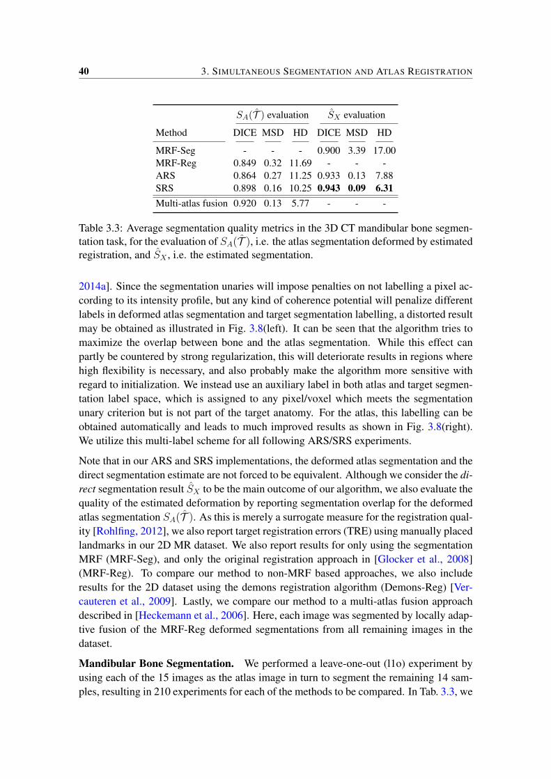
40 3. SIMULTANEOUS SEGMENTATION AND ATLAS REGISTRATION
SA(T ) evaluation SX evaluation
Method DICE MSD HD DICE MSD HD
MRF-Seg - - - 0.900 3.39 17.00MRF-Reg 0.849 0.32 11.69 - - -ARS 0.864 0.27 11.25 0.933 0.13 7.88SRS 0.898 0.16 10.25 0.943 0.09 6.31Multi-atlas fusion 0.920 0.13 5.77 - - -
Table 3.3: Average segmentation quality metrics in the 3D CT mandibular bone segmen-tation task, for the evaluation of SA(T ), i.e. the atlas segmentation deformed by estimatedregistration, and SX , i.e. the estimated segmentation.
2014a]. Since the segmentation unaries will impose penalties on not labelling a pixel ac-cording to its intensity profile, but any kind of coherence potential will penalize differentlabels in deformed atlas segmentation and target segmentation labelling, a distorted resultmay be obtained as illustrated in Fig. 3.8(left). It can be seen that the algorithm tries tomaximize the overlap between bone and the atlas segmentation. While this effect canpartly be countered by strong regularization, this will deteriorate results in regions wherehigh flexibility is necessary, and also probably make the algorithm more sensitive withregard to initialization. We instead use an auxiliary label in both atlas and target segmen-tation label space, which is assigned to any pixel/voxel which meets the segmentationunary criterion but is not part of the target anatomy. For the atlas, this labelling can beobtained automatically and leads to much improved results as shown in Fig. 3.8(right).We utilize this multi-label scheme for all following ARS/SRS experiments.
Note that in our ARS and SRS implementations, the deformed atlas segmentation and thedirect segmentation estimate are not forced to be equivalent. Although we consider the di-rect segmentation result SX to be the main outcome of our algorithm, we also evaluate thequality of the estimated deformation by reporting segmentation overlap for the deformedatlas segmentation SA(T ). As this is merely a surrogate measure for the registration qual-ity [Rohlfing, 2012], we also report target registration errors (TRE) using manually placedlandmarks in our 2D MR dataset. We also report results for only using the segmentationMRF (MRF-Seg), and only the original registration approach in [Glocker et al., 2008](MRF-Reg). To compare our method to non-MRF based approaches, we also includeresults for the 2D dataset using the demons registration algorithm (Demons-Reg) [Ver-cauteren et al., 2009]. Lastly, we compare our method to a multi-atlas fusion approachdescribed in [Heckemann et al., 2006]. Here, each image was segmented by locally adap-tive fusion of the MRF-Reg deformed segmentations from all remaining images in thedataset.
Mandibular Bone Segmentation. We performed a leave-one-out (l1o) experiment byusing each of the 15 images as the atlas image in turn to segment the remaining 14 sam-ples, resulting in 210 experiments for each of the methods to be compared. In Tab. 3.3, we
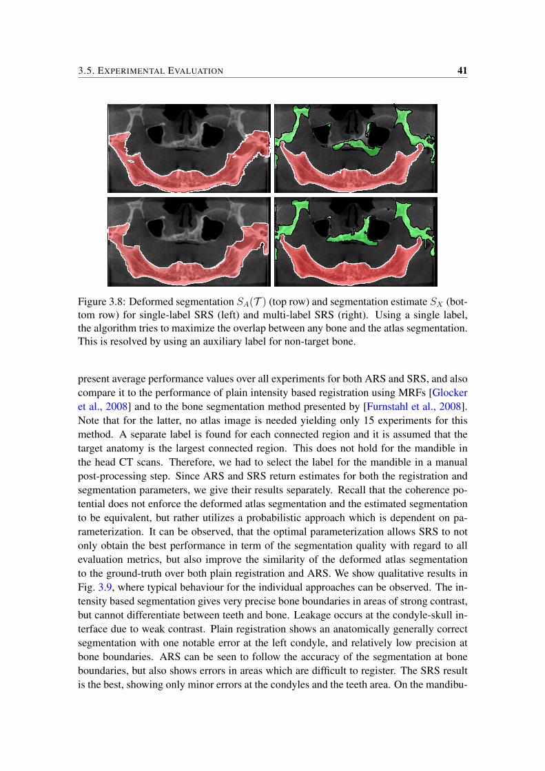
3.5. EXPERIMENTAL EVALUATION 41
Figure 3.8: Deformed segmentation SA(T ) (top row) and segmentation estimate SX (bot-tom row) for single-label SRS (left) and multi-label SRS (right). Using a single label,the algorithm tries to maximize the overlap between any bone and the atlas segmentation.This is resolved by using an auxiliary label for non-target bone.
present average performance values over all experiments for both ARS and SRS, and alsocompare it to the performance of plain intensity based registration using MRFs [Glockeret al., 2008] and to the bone segmentation method presented by [Furnstahl et al., 2008].Note that for the latter, no atlas image is needed yielding only 15 experiments for thismethod. A separate label is found for each connected region and it is assumed that thetarget anatomy is the largest connected region. This does not hold for the mandible inthe head CT scans. Therefore, we had to select the label for the mandible in a manualpost-processing step. Since ARS and SRS return estimates for both the registration andsegmentation parameters, we give their results separately. Recall that the coherence po-tential does not enforce the deformed atlas segmentation and the estimated segmentationto be equivalent, but rather utilizes a probabilistic approach which is dependent on pa-rameterization. It can be observed, that the optimal parameterization allows SRS to notonly obtain the best performance in term of the segmentation quality with regard to allevaluation metrics, but also improve the similarity of the deformed atlas segmentationto the ground-truth over both plain registration and ARS. We show qualitative results inFig. 3.9, where typical behaviour for the individual approaches can be observed. The in-tensity based segmentation gives very precise bone boundaries in areas of strong contrast,but cannot differentiate between teeth and bone. Leakage occurs at the condyle-skull in-terface due to weak contrast. Plain registration shows an anatomically generally correctsegmentation with one notable error at the left condyle, and relatively low precision atbone boundaries. ARS can be seen to follow the accuracy of the segmentation at boneboundaries, but also shows errors in areas which are difficult to register. The SRS resultis the best, showing only minor errors at the condyles and the teeth area. On the mandibu-
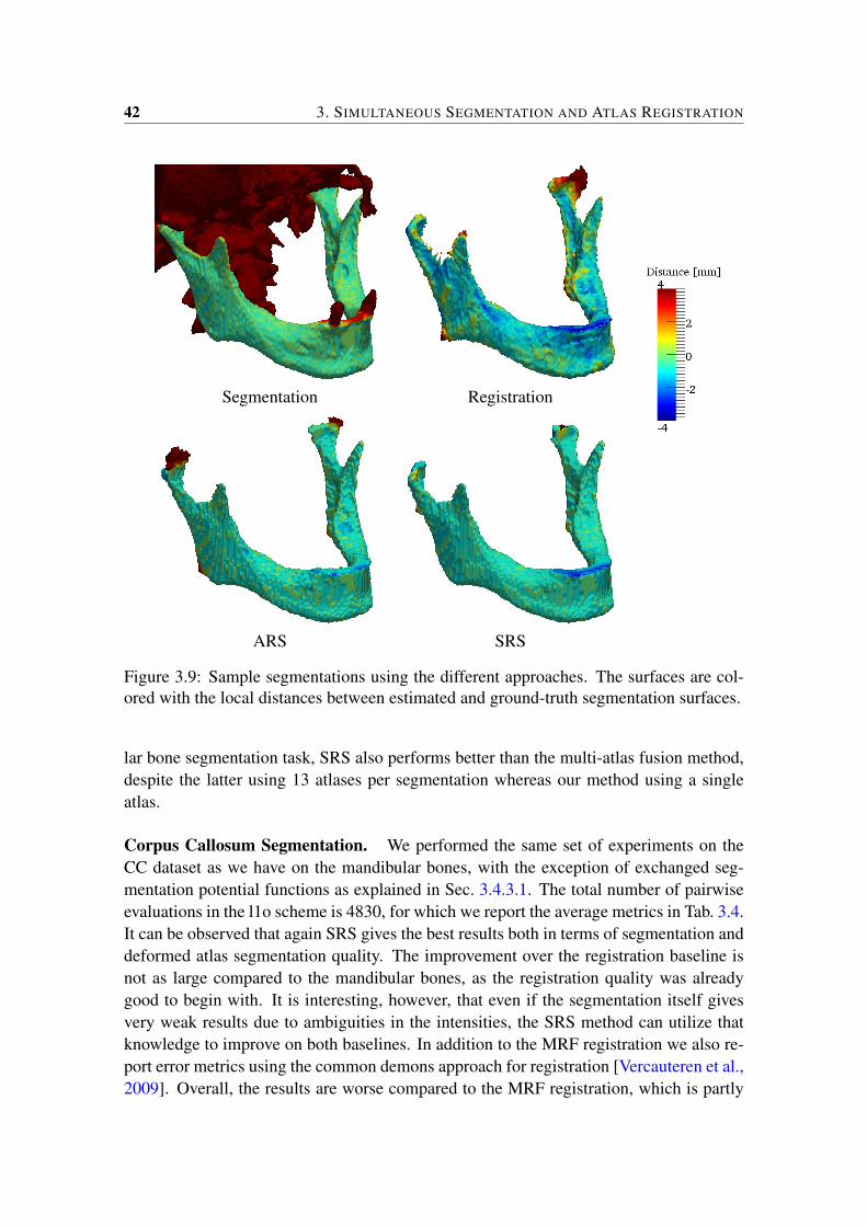
42 3. SIMULTANEOUS SEGMENTATION AND ATLAS REGISTRATION
Segmentation Registration
ARS SRS
Figure 3.9: Sample segmentations using the different approaches. The surfaces are col-ored with the local distances between estimated and ground-truth segmentation surfaces.
lar bone segmentation task, SRS also performs better than the multi-atlas fusion method,despite the latter using 13 atlases per segmentation whereas our method using a singleatlas.
Corpus Callosum Segmentation. We performed the same set of experiments on theCC dataset as we have on the mandibular bones, with the exception of exchanged seg-mentation potential functions as explained in Sec. 3.4.3.1. The total number of pairwiseevaluations in the l1o scheme is 4830, for which we report the average metrics in Tab. 3.4.It can be observed that again SRS gives the best results both in terms of segmentation anddeformed atlas segmentation quality. The improvement over the registration baseline isnot as large compared to the mandibular bones, as the registration quality was alreadygood to begin with. It is interesting, however, that even if the segmentation itself givesvery weak results due to ambiguities in the intensities, the SRS method can utilize thatknowledge to improve on both baselines. In addition to the MRF registration we also re-port error metrics using the common demons approach for registration [Vercauteren et al.,2009]. Overall, the results are worse compared to the MRF registration, which is partly
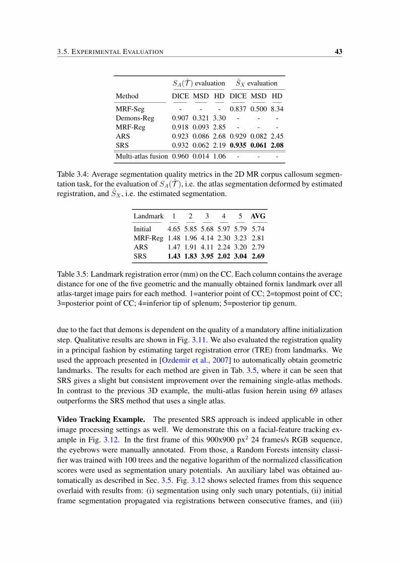
3.5. EXPERIMENTAL EVALUATION 43
SA(T ) evaluation SX evaluation
Method DICE MSD HD DICE MSD HD
MRF-Seg - - - 0.837 0.500 8.34Demons-Reg 0.907 0.321 3.30 - - -MRF-Reg 0.918 0.093 2.85 - - -ARS 0.923 0.086 2.68 0.929 0.082 2.45SRS 0.932 0.062 2.19 0.935 0.061 2.08Multi-atlas fusion 0.960 0.014 1.06 - - -
Table 3.4: Average segmentation quality metrics in the 2D MR corpus callosum segmen-tation task, for the evaluation of SA(T ), i.e. the atlas segmentation deformed by estimatedregistration, and SX , i.e. the estimated segmentation.
Landmark 1 2 3 4 5 AVG
Initial 4.65 5.85 5.68 5.97 5.79 5.74MRF-Reg 1.48 1.96 4.14 2.30 3.23 2.81ARS 1.47 1.91 4.11 2.24 3.20 2.79SRS 1.43 1.83 3.95 2.02 3.04 2.69
Table 3.5: Landmark registration error (mm) on the CC. Each column contains the averagedistance for one of the five geometric and the manually obtained fornix landmark over allatlas-target image pairs for each method. 1=anterior point of CC; 2=topmost point of CC;3=posterior point of CC; 4=inferior tip of splenum; 5=posterior tip genum.
due to the fact that demons is dependent on the quality of a mandatory affine initializationstep. Qualitative results are shown in Fig. 3.11. We also evaluated the registration qualityin a principal fashion by estimating target registration error (TRE) from landmarks. Weused the approach presented in [Ozdemir et al., 2007] to automatically obtain geometriclandmarks. The results for each method are given in Tab. 3.5, where it can be seen thatSRS gives a slight but consistent improvement over the remaining single-atlas methods.In contrast to the previous 3D example, the multi-atlas fusion herein using 69 atlasesoutperforms the SRS method that uses a single atlas.
Video Tracking Example. The presented SRS approach is indeed applicable in otherimage processing settings as well. We demonstrate this on a facial-feature tracking ex-ample in Fig. 3.12. In the first frame of this 900x900 px2 24 frames/s RGB sequence,the eyebrows were manually annotated. From those, a Random Forests intensity classi-fier was trained with 100 trees and the negative logarithm of the normalized classificationscores were used as segmentation unary potentials. An auxiliary label was obtained au-tomatically as described in Sec. 3.5. Fig. 3.12 shows selected frames from this sequenceoverlaid with results from: (i) segmentation using only such unary potentials, (ii) initialframe segmentation propagated via registrations between consecutive frames, and (iii)
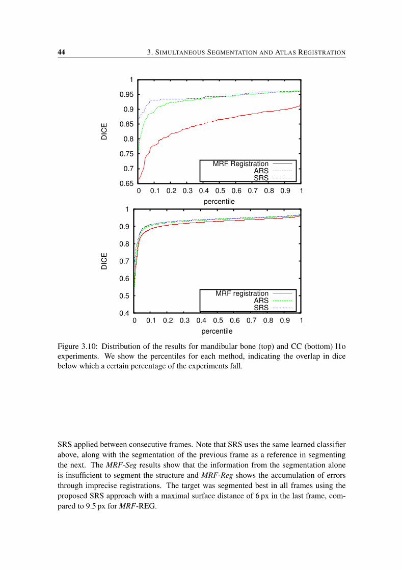
44 3. SIMULTANEOUS SEGMENTATION AND ATLAS REGISTRATION
0.65
0.7
0.75
0.8
0.85
0.9
0.95
1
0 0.1 0.2 0.3 0.4 0.5 0.6 0.7 0.8 0.9 1
DIC
E
percentile
MRF RegistrationARSSRS
0.4
0.5
0.6
0.7
0.8
0.9
1
0 0.1 0.2 0.3 0.4 0.5 0.6 0.7 0.8 0.9 1
DIC
E
percentile
MRF registrationARSSRS
Figure 3.10: Distribution of the results for mandibular bone (top) and CC (bottom) l1oexperiments. We show the percentiles for each method, indicating the overlap in dicebelow which a certain percentage of the experiments fall.
SRS applied between consecutive frames. Note that SRS uses the same learned classifierabove, along with the segmentation of the previous frame as a reference in segmentingthe next. The MRF-Seg results show that the information from the segmentation aloneis insufficient to segment the structure and MRF-Reg shows the accumulation of errorsthrough imprecise registrations. The target was segmented best in all frames using theproposed SRS approach with a maximal surface distance of 6 px in the last frame, com-pared to 9.5 px for MRF-REG.
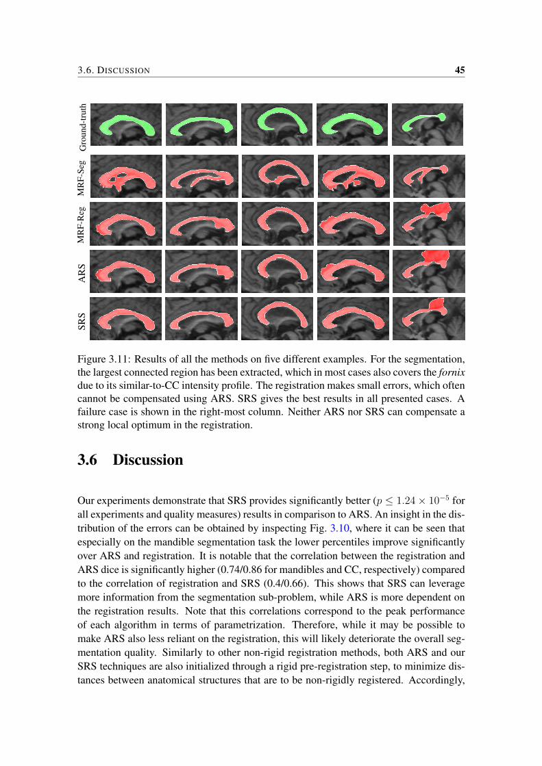
3.6. DISCUSSION 45G
roun
d-tr
uth
MR
F-Se
gM
RF-
Reg
AR
SSR
S
Figure 3.11: Results of all the methods on five different examples. For the segmentation,the largest connected region has been extracted, which in most cases also covers the fornixdue to its similar-to-CC intensity profile. The registration makes small errors, which oftencannot be compensated using ARS. SRS gives the best results in all presented cases. Afailure case is shown in the right-most column. Neither ARS nor SRS can compensate astrong local optimum in the registration.
3.6 Discussion
Our experiments demonstrate that SRS provides significantly better (p ≤ 1.24× 10⁻⁵ forall experiments and quality measures) results in comparison to ARS. An insight in the dis-tribution of the errors can be obtained by inspecting Fig. 3.10, where it can be seen thatespecially on the mandible segmentation task the lower percentiles improve significantlyover ARS and registration. It is notable that the correlation between the registration andARS dice is significantly higher (0.74/0.86 for mandibles and CC, respectively) comparedto the correlation of registration and SRS (0.4/0.66). This shows that SRS can leveragemore information from the segmentation sub-problem, while ARS is more dependent onthe registration results. Note that this correlations correspond to the peak performanceof each algorithm in terms of parametrization. Therefore, while it may be possible tomake ARS also less reliant on the registration, this will likely deteriorate the overall seg-mentation quality. Similarly to other non-rigid registration methods, both ARS and ourSRS techniques are also initialized through a rigid pre-registration step, to minimize dis-tances between anatomical structures that are to be non-rigidly registered. Accordingly,
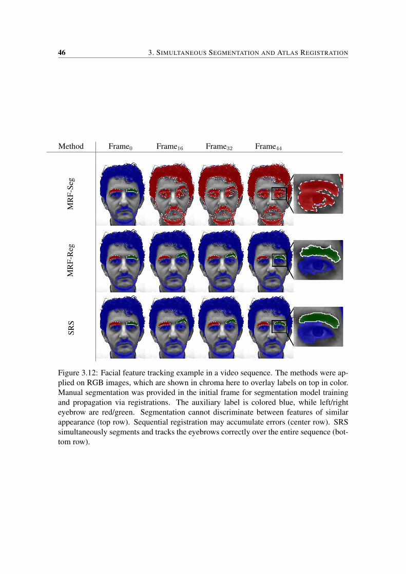
46 3. SIMULTANEOUS SEGMENTATION AND ATLAS REGISTRATION
Method Frame0 Frame16 Frame32 Frame44
MR
F-Se
gM
RF-
Reg
SRS
Figure 3.12: Facial feature tracking example in a video sequence. The methods were ap-plied on RGB images, which are shown in chroma here to overlay labels on top in color.Manual segmentation was provided in the initial frame for segmentation model trainingand propagation via registrations. The auxiliary label is colored blue, while left/righteyebrow are red/green. Segmentation cannot discriminate between features of similarappearance (top row). Sequential registration may accumulate errors (center row). SRSsimultaneously segments and tracks the eyebrows correctly over the entire sequence (bot-tom row).

3.6. DISCUSSION 47
the capture range of such a deformable registration can be perceived as the likelihood ofreaching a satisfactory local optimum. This is indeed what we believe as one of the ma-jor reasons behind why SRS provides a significant improvement over ARS. Even thoughboth methods have the same theoretical deformation range, the distance-based segmenta-tion information provided to SRS by its coherence potential is seen to improve the fidelityof such achieved local optimum.
Formally, the computational complexity of our SRS implementation can be divided intothree parts: (i) computation of registration unary potentials, and (ii) computation of dis-tance transforms, (iii) solution of MRF using alpha-expansion graph-cuts. An upperbound for the first is O(rga), where r=|LR| is the number of registration labels, g isthe number of nodes in the registration graph G and a is the size of the local supportarea defined by η. The computation time of the registration unaries was reduced con-siderably by using efficient similarity metrics such as local normalized cross correlation(LNCC) [Cachier et al., 2003], which uses convolution with Gaussian kernels. The dis-tance transform of each segmentation label can be computed in linear time with respect tothe number of pixels N in the image, resulting in a complexity of O(Ns), where s=|LS|is the number of segmentation labels. α-expansion in general needs O(lBiα) run-time,where l is the number of labels, B is the complexity of a binary graph-cut, and iα is thenumber of required alpha-expansion iterations (typically about three). Since the binarygraphs to be solved in SRS differ depending on whether a segmentation or a registra-tion label is expanded, we describe the complexity as O(iα(sBS + rBR)), where sub-scripts R and S denote the registration and segmentation sub-domains, respectively. BS
is O(N2CS), where CS is the cost of the minimal cut and BR is analogously O(g2CR).This needs to be solved multiple times for each multi-resolution level, where the last levelwill have the highest complexity. Therefore, an upper bound to the complexity of SRS isgiven by
O(mimax(rgmaxamax + s+ iα(sN2CS + rg2CR))),
where m is the number of multi-resolution levels, imax is the maximum number of itera-tions at that level, and gmax and amax are the maximal sizes of, respectively, registrationgraph and local support area at the highest multi-resolution level.
Although neither [Mahapatra and Sun, 2012] nor [Parisot et al., 2012] performs SRSusing an atlas segmentation, they both use discrete MRFs to solve simultaneous seg-mentation and registration problems. Therefore, below we compare our method to thosefrom an algorithmic viewpoint, where the main distinction is their use of the full prod-uct label space LT × LS . While this may facilitate a joint regularization of segmentationand registration [Mahapatra and Sun, 2012] or an adaptive thresholding of registrationsimilarity [Parisot et al., 2012], it raises two main difficulties. First is the substantiallylarger label space. For example, dense displacement sampling in 2D with 7 samples peraxis and ten segmentation labels yields 72 · 10 = 490 labels in the product label space,while only 72 + 10 = 59 labels in the sum label space used by our SRS implementation.Since the complexity of discrete optimization algorithms depends on the number of labels
48 3. SIMULTANEOUS SEGMENTATION AND ATLAS REGISTRATION
(e.g. alpha expansions complexity is linear with the number of labels), this greatly ef-fects computational efficiency. Second is the use of one single grid for both segmentationand registration. For the task of [Mahapatra and Sun, 2012] to improve fine registrationof time-series images, a high resolution (pixel-level) control grid is used, requiring over5 min per iteration for our 2D images, compared to ≈1 min runtime for our entire seg-mentation/registration. To avoid tearing, hard-constraints were used in [Mahapatra andSun, 2012] such that the difference between neighboring displacements should be smallerthan
√3 pixel. However, not only that folding can still occur when deformations from
succeeding iterations are composed, but also a dense registration label space is requiredto allow sufficient deformation flexibility, which in turn would yield an infeasible numberof labels for our application. For instance, for the same displacement range (60 pixel or20 mm) as in our 2D experiments, (2 ∗ 60 + 1)2 = 14641 registration labels would beneeded. In contrast, [Parisot et al., 2012] uses the multi-resolution hierarchy of [Glockeret al., 2008], where segmentation labels are assigned at the same resolution as the regis-tration grid. Therefore, at initial coarse levels to allow for large displacements, the coarsesegmentation resolution does not allow small structures to be detected. We implementedthis in our algorithm by fixing the segmentation grid resolution to the registration grid res-olution. On the 2D dataset, this yielded a DICE coefficient of 0.8 which is significantlyworse than any reported result in Tab. 3.4.
SRS using a fixed number of iterations is also faster compared to ARS. Indeed, the fullSRS optimization runs under 2 min in 2D and 50 min in 3D on average with an ITK im-plementation in C++ on an Intel Core i7 1.6GHz processor. In comparison, one ARSiteration takes 0.5 min in 2D, 13 min in 3D and does often not converge in 10 iterations,causing it to be slower on average. Still, such run-time requirements can be seen as alimiting factor of our SRS method. However, other methods to achieve similar perfor-mance may require similar run-time in the form of multiple non-rigid registrations, ontop of additional manual labor to generate a larger amount of prior knowledge. This isdemonstrated in our comparison of SRS to multi-atlas fusion, which is the state-of-the-artin image segmentation [Rohlfing et al., 2005, Heckemann et al., 2006]. While multi-atlasfusion outperforms SRS on the 2D MRI data, 69 atlas segmentations were fused to seg-ment one image. This amount of prior knowledge is hard to obtain in clinical scenarios.In contrast, on the 3D CT bone segmentation task, the amount of prior knowledge is morelimited (14 fused segmentations per target). Here, it can be seen that SRS outperformsmulti-atlas fusion with regard to volume overlap and mean surface distance, while beingslightly less robust in terms of Hausdorff distance. This can be attributed to the difficultregistration procedure caused by different anatomies and artifacts caused by dental im-plants on the one side, and intensity based bone segmentation being a well defined taskon the other side. While multi-atlas fusion can only rely on the difficult registrations, SRSis able to successfully combine segmentation and registration information, which yieldsvery good results despite using an order of magnitude less prior knowledge.

3.7. CONCLUSIONS 49
3.7 Conclusions
In this work, we have presented a novel approach for simultaneous registration and seg-mentation (SRS). We have employed a Bayesian derivation to obtain a formulation of thesimultaneous model, which can be solved using discrete MRFs on a control grid hierar-chy. The solution for each MRF is found efficiently by using alpha-expansion graph-cuts.Making use of multi-resolution non-rigid registration in conjunction with pixel-level seg-mentation, our method allows a precise, robust segmentation of target images using onlya single atlas image. We show experimentally that SRS is more accurate and less depen-dent on the registration in comparison to an iterative optimization using the same criterion.Theoretically, our method estimates all parameters simultaneously using the proposed for-mulation in this paper. However, memory requirements make a hierarchical displacementrefinement approach necessary, which is solved using a sequence of MRFs. In the future,we plan to address this implementation constraint. We also envision increased perfor-mance by using classifiers which can make use of context, e.g. local shape, contrast andtexture.

4Semi-supervised Segmentation UsingMultiple Segmentation Hypothesesfrom a Single Atlas
A semi-supervised segmentation method using a single atlas is presented in this paper.Traditional atlas-based segmentation suffers from either a strong bias towards the se-lected atlas or the need for manual effort to create multiple atlas images. Similar tosemi-supervised learning in computer vision, we study a method which exploits informa-tion contained in a set of unlabelled images by mutually registering them non-rigidly andpropagating the single atlas segmentation over multiple such registration paths to eachtarget. These multiple segmentation hypotheses are then fused by local weighting basedon registration similarity. Our results on two datasets of different anatomies and imagemodalities, corpus callosum MR and mandible CT images, show a significant improve-ment in segmentation accuracy compared to traditional single atlas based segmentation.We also show that the bias towards the selected atlas is minimized using our method.Additionally, we devise a method for the selection of intermediate targets used for prop-agation, in order to reduce the number of necessary inter-target registrations without lossof final segmentation accuracy.
4.1 Introduction
Image segmentation is an essential problem in medical image processing. Among au-tomatic segmentation methods, the amount of prior information needed is a major dis-tinguishing characteristic of different approaches. It is desirable to limit the constraintsposed by prior knowledge both to retain generalizability and to reduce the effort required
This chapter has been published as: Gass, T., Szekely, G., and Goksel, O. (2012). Semi-supervisedSegmentation Using Multiple Segmentation Hypotheses from a Single Atlas. In Proc. MICCAI Workshopon Medical Computer Vision, pages 29–37
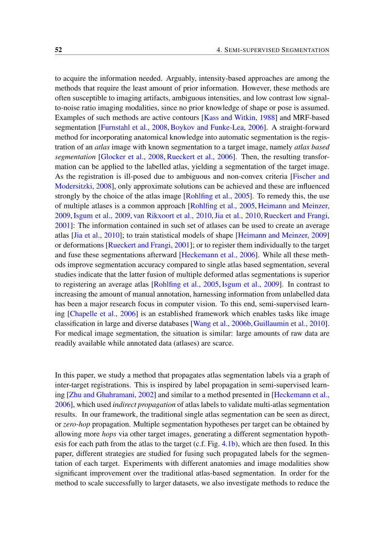
52 4. SEMI-SUPERVISED SEGMENTATION
to acquire the information needed. Arguably, intensity-based approaches are among themethods that require the least amount of prior information. However, these methods areoften susceptible to imaging artifacts, ambiguous intensities, and low contrast low signal-to-noise ratio imaging modalities, since no prior knowledge of shape or pose is assumed.Examples of such methods are active contours [Kass and Witkin, 1988] and MRF-basedsegmentation [Furnstahl et al., 2008, Boykov and Funke-Lea, 2006]. A straight-forwardmethod for incorporating anatomical knowledge into automatic segmentation is the regis-tration of an atlas image with known segmentation to a target image, namely atlas basedsegmentation [Glocker et al., 2008, Rueckert et al., 2006]. Then, the resulting transfor-mation can be applied to the labelled atlas, yielding a segmentation of the target image.As the registration is ill-posed due to ambiguous and non-convex criteria [Fischer andModersitzki, 2008], only approximate solutions can be achieved and these are influencedstrongly by the choice of the atlas image [Rohlfing et al., 2005]. To remedy this, the useof multiple atlases is a common approach [Rohlfing et al., 2005, Heimann and Meinzer,2009, Isgum et al., 2009, van Rikxoort et al., 2010, Jia et al., 2010, Rueckert and Frangi,2001]: The information contained in such set of atlases can be used to create an averageatlas [Jia et al., 2010]; to train statistical models of shape [Heimann and Meinzer, 2009]or deformations [Rueckert and Frangi, 2001]; or to register them individually to the targetand fuse these segmentations afterward [Heckemann et al., 2006]. While all these meth-ods improve segmentation accuracy compared to single atlas based segmentation, severalstudies indicate that the latter fusion of multiple deformed atlas segmentations is superiorto registering an average atlas [Rohlfing et al., 2005, Isgum et al., 2009]. In contrast toincreasing the amount of manual annotation, harnessing information from unlabelled datahas been a major research focus in computer vision. To this end, semi-supervised learn-ing [Chapelle et al., 2006] is an established framework which enables tasks like imageclassification in large and diverse databases [Wang et al., 2006b,Guillaumin et al., 2010].For medical image segmentation, the situation is similar: large amounts of raw data arereadily available while annotated data (atlases) are scarce.
In this paper, we study a method that propagates atlas segmentation labels via a graph ofinter-target registrations. This is inspired by label propagation in semi-supervised learn-ing [Zhu and Ghahramani, 2002] and similar to a method presented in [Heckemann et al.,2006], which used indirect propagation of atlas labels to validate multi-atlas segmentationresults. In our framework, the traditional single atlas segmentation can be seen as direct,or zero-hop propagation. Multiple segmentation hypotheses per target can be obtained byallowing more hops via other target images, generating a different segmentation hypoth-esis for each path from the atlas to the target (c.f. Fig. 4.1b), which are then fused. In thispaper, different strategies are studied for fusing such propagated labels for the segmen-tation of each target. Experiments with different anatomies and image modalities showsignificant improvement over the traditional atlas-based segmentation. In order for themethod to scale successfully to larger datasets, we also investigate methods to reduce the
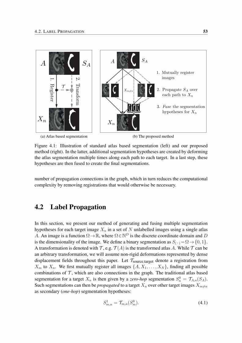
4.2. LABEL PROPAGATION 53
Xn
2.Tran
sformg
1.Register
T
SAA
(a) Atlas based segmentation
Xm =n
1. Mutually registerimages
2. Propagate SA overeach path to Xn
3. Fuse the segmentationhypotheses for Xn
Xn
A SA
(b) The proposed method
Figure 4.1: Illustration of standard atlas based segmentation (left) and our proposedmethod (right). In the latter, additional segmentation hypotheses are created by deformingthe atlas segmentation multiple times along each path to each target. In a last step, thesehypotheses are then fused to create the final segmentations.
number of propagation connections in the graph, which in turn reduces the computationalcomplexity by removing registrations that would otherwise be necessary.
4.2 Label Propagation
In this section, we present our method of generating and fusing multiple segmentationhypotheses for each target image Xn in a set of N unlabelled images using a single atlasA. An image is a function Ω→R, where Ω∈ND is the discrete coordinate domain and Dis the dimensionality of the image. We define a binary segmentation as S( · ) =Ω→0, 1.A transformation is denoted with T , e.g. T (A) is the transformed atlasA. While T can bean arbitrary transformation, we will assume non-rigid deformations represented by densedisplacement fields throughout this paper. Let Tsource,target denote a registration fromXm to Xn. We first mutually register all images A,X1, . . . , XN, finding all possiblecombinations of T , which are also connections in the graph. The traditional atlas basedsegmentation for a target Xn is then given by a zero-hop segmentation S0
n = TA,n(SA).Such segmentations can then be propagated to a targetXn over other target imagesXm6=nas secondary (one-hop) segmentation hypotheses:
S1m,n = Tm,n(S0
m). (4.1)

54 4. SEMI-SUPERVISED SEGMENTATION
These hypotheses must then be fused: We use a function F to first generate a spatialsegmentation probability map Sn = Ω → [0, 1] and subsequently binarize this usingthresholding. The said probability map is generated as a weighted average of the zero-and one-hop segmentation hypotheses:
Sn = F(S0n, S1
m,n|m 6= n)
=1∑λ
(λ0nS
0n +
∑m 6=n
λ1m,nS
1m,n
). (4.2)
We propose and evaluate two different strategies for the choice of weights λ:
Global Similarity Weighting (GSW) : Assuming correlation between segmentation ac-curacy and a normalized post-registration similarity fG, the latter can be used as a scalarweight. Using the zero-hop deformed atlas image A0
n=TA,n(A) , the zero-hop weight isthen λ0
n=fG(Xn, A0n) . The atlas image is propagated analogously to the atlas segmentation
along each path, i.e. A1m,n= Tm,n(A0
m) , which leads to one-hop weights as follows:
λ1m,n = fG
(Xn, A
1m,n
). (4.3)
Locally Adaptive Weighting (LAW) : In contrast to the constant weights per hypothesisin GSW, a spatially-varying local weighting scheme is used:
λ1m,n(p) = fL
(Xn(p), A1
m,n(p)),∀p ∈ Ω . (4.4)
In contrast to GSW, such locally adaptive weighting is expected to leverage useful infor-mation even from partially mis-registered images.
4.3 Compact Graphs
To use all one-hop segmentation hypotheses, all graph connections should be computedrequiring N2 registrations. With large datasets this may easily become computationallychallenging. Below, different methods are proposed for selecting a target image subset X,called support-samples, that will act as intermediate nodes via which the atlas segmen-tation is propagated using (4.1). Reducing the size K=|X| then decrease the number ofedges in G and hence the number of necessary inter-target registrations. A natural choiceis to sort nodes by their GSW-based zero-hop weights λ0
n, as this corresponds to imagesimilarity to deformed atlas, and to use the highest ranked images as support samples. Wecall this GSW-based ranking. This scheme makes two assumptions: first, that it is utmostimportant to propagate ‘good’ zero-hop segmentations; and second, that the quality ofthese segmentations can be assessed reliably using the similarity function f . Using our

4.4. RESULTS AND DISCUSSION 55
label propagation framework, we propose the following two additional ranking criteriafor selecting support samples.
In segmenting a target Xn, we wish to quantify how reliable a one-hop segmentationhypotesis S1
m,n via an intermediate node Xm is. As we only know the segmentation ofthe atlas, we define an atlas reconstruction error (ARE) for such quantification. Ex-ploiting the fact that most non-rigid registration algorithms are not symmetric, we com-pute deformations Tm,A to obtain back-propagated one-hop atlas segmentation hypothesesS1m,A=Tm,A(S0
m) via each graph node. Then, ARE for each node is defined based on Dice’ssimilarity coefficient:
ARE (m) = 1− Dice(SA, S
1m,A
), (4.5)
and support samples are selected from the smallest error nodes. While such ranking isexpected to perform superior to GSW-based ranking, it cannot ensure that complementaryinformation is contained in the set. For example, a subset X might have individually lowAREs, however, their one-hop hypotheses may all contain similar errors which are thenamplified when they are fused to create a target segmentation. It is thus desirable to finda complementary basis, where each support sample is likely to contain information thatother samples do not provide. We therefore propose a groupwise error criterion (ARE-G)to score a set of K graph nodes:
ARE-G(SA, m1, . . . ,mK) = 1− Dice(SA, F
(S1m1,A
, . . . , S1mK ,A
)), (4.6)
where F is the fusion function in (4.2). As it is not feasible to evaluate all(NK
)K-sized sets
of support samples, we rely on a greedy scheme where we pick the first support samplebased on its individual ARE, and iteratively add support samples that reduce ARE-G themost.
4.4 Results and Discussion
We evaluated our method using a set of 70 mid-saggital slices of MR brain scans con-taining the corpus callosum and a set of 15 3D CT scans of the head. Both datasets wererigidly pre-aligned. In the MR dataset a fixed region of interest containing the corpuscallosum was cropped out in all images. The images are 120x200 pixels with 0.3 mmspacing in the MR dataset and 160x160x129 voxels with 1 mm spacing in the CT dataset.We used the Dice coefficient to measure volume overlap, the Hausdorff distance (HD) forestimating maximum surface-to-surface distance, and the mean surface distance (MSD)as an additional distance based metric. In both datasets we performed a leave-one-out(l1o) evaluation scheme, using each image as atlas in turn to segment all remaining im-ages. We used our own implementation of the MRF-based registration in [Glocker et al.,2008] as the registration method of choice in our experiments. We used normalized cross
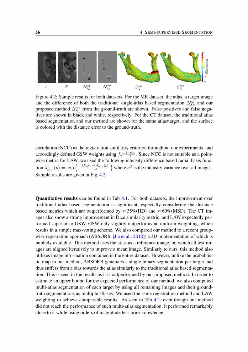
56 4. SEMI-SUPERVISED SEGMENTATION
A X ∆tradSX
∆propSX
S tradX Sprop
X
MR
6
4
2
0
2
4
6
Dista
nce
[mm
]
Figure 4.2: Sample results for both datasets. For the MR dataset, the atlas, a target imageand the difference of both the traditional single-atlas based segmentation ∆trad
SXand our
proposed method ∆propSX
from the ground-truth are shown. False positives and false nega-tives are shown in black and white, respectively. For the CT dataset, the traditional atlasbased segmentation and our method are shown for the same atlas/target, and the surfaceis colored with the distance error to the ground-truth.
correlation (NCC) as the registration similarity criterion throughout our experiments, andaccordingly defined GSW weights using fG=1−NCC
2. Since NCC is not suitable as a point-
wise metric for LAW, we used the following intensity difference based radial basis func-tion λ1
m,n(p) = exp(− |Xn(p)−A1
m,n(p)|σ2
)where σ2 is the intensity variance over all images.
Sample results are given in Fig. 4.2.
Quantitative results can be found in Tab. 4.1. For both datasets, the improvement overtraditional atlas based segmentation is significant, especially considering the distancebased metrics which are outperformed by ≈ 35%(HD) and ≈ 60%(MSD). The CT im-ages also show a strong improvement in Dice similarity metric, and LAW expectedly per-formed superior to GSW. GSW only slightly outperforms an uniform weighting, whichresults in a simple max-voting scheme. We also compared our method to a recent group-wise registration approach (ABSORB [Jia et al., 2010]) a 3D implementation of which ispublicly available. This method uses the atlas as a reference image, on which all test im-ages are aligned iteratively to improve a mean image. Similarly to ours, this method alsoutilizes image information contained in the entire dataset. However, unlike the probablis-tic map in our method, ABSORB generates a single binary segmentation per target andthus suffers from a bias towards the atlas similarly to the traditional atlas based segmenta-tion. This is seen in the results as it is outperformed by our proposed method. In order toestimate an upper bound for the expected performance of our method, we also computedmulti-atlas segmentation of each target by using all remaining images and their ground-truth segmentations as multiple atlases. We used the same registration method and LAWweighting to achieve comparable results. As seen in Tab. 4.1, even though our methoddid not reach the performance of such multi-atlas segmentation, it performed remarkablyclose to it while using orders of magnitude less prior knowledge.
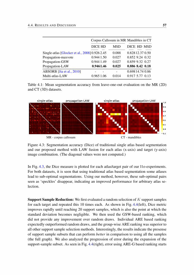
4.4. RESULTS AND DISCUSSION 57
Corpus Callosum in MR Mandibles in CT
DICE HD MSD DICE HD MSD
Single-atlas [Glocker et al., 2008] 0.926 2.45 0.088 0.82812.37 0.50Propagation-maxvote 0.944 1.50 0.027 0.852 9.24 0.32Propagation-GSW 0.944 1.49 0.027 0.859 9.32 0.27Propagation-LAW 0.9461.46 0.025 0.886 8.42 0.18ABSORB [Jia et al., 2010] - - - 0.69814.74 0.86Multi-atlas-LAW 0.965 1.06 0.014 0.917 5.77 0.13
Table 4.1: Mean segmentation accuracy from leave-one-out evaluation on the MR (2D)and CT (3D) datasets.
MR - corpus callosum CT - mandibles
Figure 4.3: Segmentation accuracy (Dice) of traditional single atlas based segmentationand our proposed method with LAW fusion for each atlas (x-axis) and target (y-axis)image combination. (The diagonal values were not computed.)
In Fig. 4.3, the Dice measure is plotted for each atlas/target pair of our l1o-experiments.For both datasets, it is seen that using traditional atlas based segmentation some atlaseslead to sub-optimal segmentations. Using our method, however, these sub-optimal pairsseen as ‘speckles’ disappear, indicating an improved performance for arbitrary atlas se-lection.
Support Sample Reduction: We first evaluated a random selection ofK support samplesfor each target and repeated this 10 times each. As shown in Fig. 4.4(left), Dice metricimproves rapidly until reaching 20 support samples, which is also the point at which thestandard deviation becomes negligible. We then used the GSW-based ranking, whichdid not provide any improvement over random draws. Individual ARE based rankingexpectedly outperformed random draws, and the group-wise ARE ranking was superior toall other support sample selection methods. Interestingly, the results indicate the presenseof support sample subsets that can perform better in comparison to using all the samples(the full graph). We also analyzed the progression of error during the expansion of thesupport-sample subset. As seen in Fig. 4.4(right), error using ARE-G based ranking starts
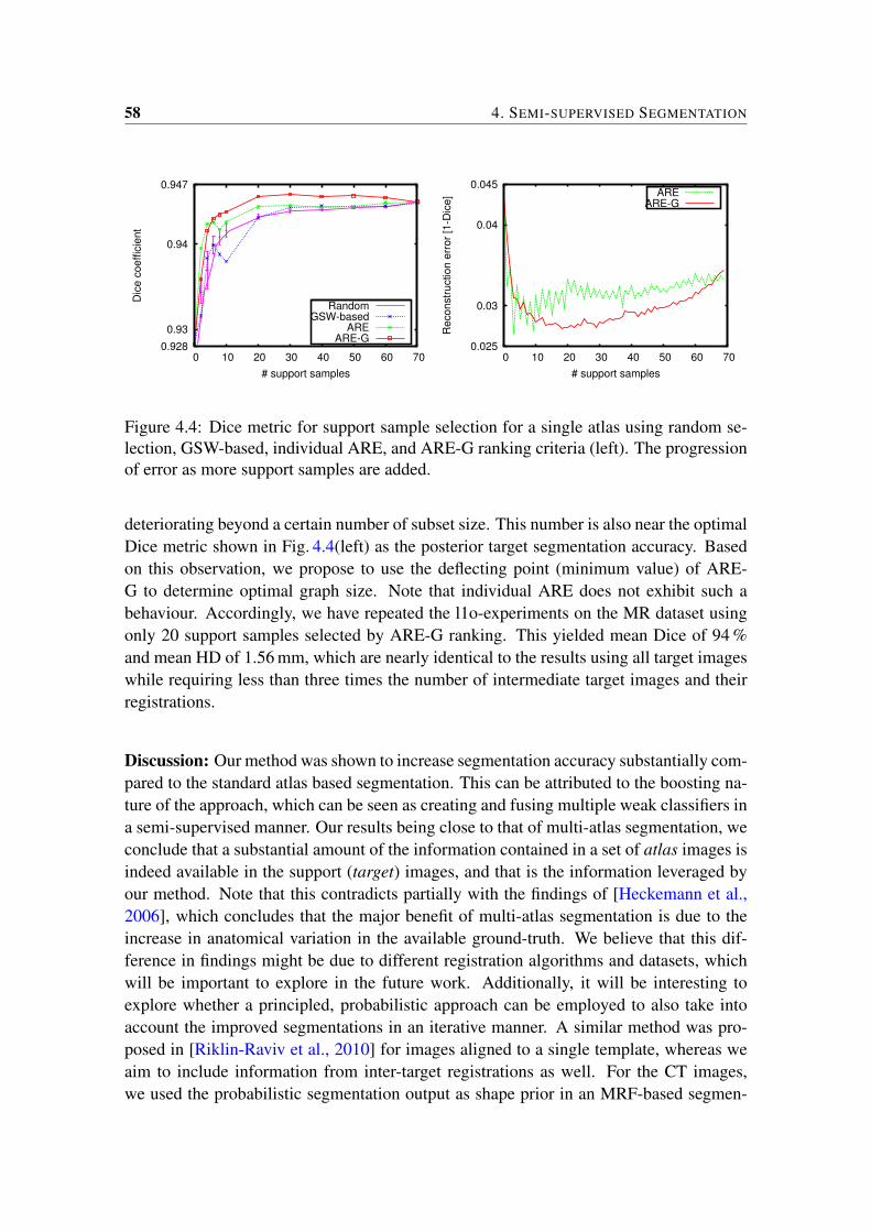
58 4. SEMI-SUPERVISED SEGMENTATION
0.928
0.93
0.94
0.947
0 10 20 30 40 50 60 70
Dic
e c
oe
ffic
ien
t
# support samples
RandomGSW-based
AREARE-G
0.025
0.03
0.04
0.045
0 10 20 30 40 50 60 70
Re
co
nstr
uctio
n e
rro
r [1
-Dic
e]
# support samples
AREARE-G
Figure 4.4: Dice metric for support sample selection for a single atlas using random se-lection, GSW-based, individual ARE, and ARE-G ranking criteria (left). The progressionof error as more support samples are added.
deteriorating beyond a certain number of subset size. This number is also near the optimalDice metric shown in Fig. 4.4(left) as the posterior target segmentation accuracy. Basedon this observation, we propose to use the deflecting point (minimum value) of ARE-G to determine optimal graph size. Note that individual ARE does not exhibit such abehaviour. Accordingly, we have repeated the l1o-experiments on the MR dataset usingonly 20 support samples selected by ARE-G ranking. This yielded mean Dice of 94 %and mean HD of 1.56 mm, which are nearly identical to the results using all target imageswhile requiring less than three times the number of intermediate target images and theirregistrations.
Discussion: Our method was shown to increase segmentation accuracy substantially com-pared to the standard atlas based segmentation. This can be attributed to the boosting na-ture of the approach, which can be seen as creating and fusing multiple weak classifiers ina semi-supervised manner. Our results being close to that of multi-atlas segmentation, weconclude that a substantial amount of the information contained in a set of atlas images isindeed available in the support (target) images, and that is the information leveraged byour method. Note that this contradicts partially with the findings of [Heckemann et al.,2006], which concludes that the major benefit of multi-atlas segmentation is due to theincrease in anatomical variation in the available ground-truth. We believe that this dif-ference in findings might be due to different registration algorithms and datasets, whichwill be important to explore in the future work. Additionally, it will be interesting toexplore whether a principled, probabilistic approach can be employed to also take intoaccount the improved segmentations in an iterative manner. A similar method was pro-posed in [Riklin-Raviv et al., 2010] for images aligned to a single template, whereas weaim to include information from inter-target registrations as well. For the CT images,we used the probabilistic segmentation output as shape prior in an MRF-based segmen-
4.5. CONCLUSIONS 59
tation [Furnstahl et al., 2008]. This led to a considerable improvement in results with amean Dice of 93 %. As this relies on strong edges to find bone boundaries, it does notyield a significant improvement in the MR images.
4.5 Conclusions
We presented a novel method that augments single-atlas based segmentation using multi-ple segmentation hypotheses for each target obtained by propagating atlas segmentationalong different paths. This outperforms both the traditional single-atlas based registrationand group-wise registration. We also demonstrated that a smaller set of support samplesproviding complementary information can be found automatically. Using such reducedset of support samples both decreases the computational complexity of the method andimproves the results as redundant and possibly detrimental information is then discarded.

5Registration Fusion using MarkovRandom Fields
Image registration is a ubiquitous technique in medical imaging. However, finding cor-respondences reliably between images is a difficult task since the registration problemis ill-posed and registration algorithms are only capable of finding local optima. Thismakes it challenging to find a suitable registration method and parametrization for a spe-cific application. To alleviate such problems, multiple registrations can be fused which istypically done by weighted averaging, which is sensitive to outliers and can not guaranteethat registrations improve. In contrast, in this work we present a Markov random fieldbased technique which fuses registrations by explicitly minimizing local dissimilaritiesof deformed source and target image, while penalizing non-smooth deformations. Weadditionally propose a registration propagation technique which combines multiple reg-istration hypotheses which are obtained from different indirect paths in a set of mutuallyregistered images. Our fused registrations are experimentally shown to improve pair-wisecorrespondences in terms of average deformation error (ADE) and target registration error(TRE) as well as improving post-registration segmentation overlap.
5.1 Introduction
Image registration is at the core of a multitude of medical image analysis techniques. It en-ables ubiquitous methods such as atlas generation, atlas-based segmentation, multi-modalinformation fusion, pre-operative planning and intra-operative guidance. High registra-tion reliability and accuracy are critical for the success of any applied method. However,it is well known that the registration problem is ill-posed [Fischer and Modersitzki, 2008]when anatomical correspondences are established using image similarity. Artefacts fromthe imaging process (noise, bias) and from discretizing the continuous spatial domain into
This chapter has been published as: Gass, T., Szekely, G., and Goksel, O. (2014d). Registration Fusionusing Markov Random Fields. In Biomedical Image Registration, page to appear
62 5. REGISTRATION FUSION USING MARKOV RANDOM FIELDS
pixels/voxels further complicate the image registration process. Numerous techniqueshave been developed to cope with these challenges. Firstmost, registration algorithmstypically include regularization terms that penalize anatomically unreasonable deforma-tions such as due to folding or tearing. For example, Markov random field (MRF) basedregistration penalizes deformations with large Euclidean distance between displacementsof neighboring points [Glocker et al., 2008]. Other approaches include Gaussian smooth-ing of velocity and update fields [Thirion, 1998], or they restrict the type of deformationto be diffeomorphic (smoothly invertable) [Vercauteren et al., 2009]. A comprehensiveoverview of registration regularization is given in [Cachier and Ayache, 2001]. Higher-level prior knowledge can also be used to regularize registration algorithm. For example,it is reasonable to expect that the outcome of registering image A to B should be thesame as inverting the registration from B to A. Such registration symmetry has beensuccesfully enforced for example in the demons [Vercauteren et al., 2008] and SyN reg-istration algorithms [Avants et al., 2008a]. One key challenge of regularized registrationis that the resulting elastic matching problem is NP-complete [Keysers and Unger, 2003]and therefore solutions can be found only approximatively, typically following the gra-dient of the objective function. To avoid poor local optima in such optimizations, mostnon-rigid registration methods require a suitable initialisation from another robust rigidor affine registration algorithm. Multi-resolution pyramids are frequently used to preventalgorithms from falling into local minima due to fine detail in early stages of the registra-tion [Rueckert et al., 1999]. Despite these advances, medical image registration is still anopen problem.
It is known from information theory that many weak information sources can be combinedinto strong information for example via boosting [Schapire, 1990]. This is reflected by thetrend in medical image segmentation, where state-of-the art results are achieved by fusingsegmentation hypotheses obtained from multiple atlases [Heckemann et al., 2006]. Opti-cal flow can computed by fusing multiple hypotheses using a mixed continuous-discreteapproach [Lempitsky et al., 2008]. There also exist studies that present methods to fusemultiple hypotheses for landmark detection [Iglesias and Karssemeijer, 2009, Santemizet al., 2013], which can be seen as a sparse registration problem. Some of the fusionmethods are specific to the chosen detection method, for example choosing landmarksbased on the cumulative score of multiple support vector machines that are independentlytrained [Santemiz et al., 2013]. A more general technique was presented in [Iglesias andKarssemeijer, 2009], where multiple landmark hypotheses obtained from different atlaseswere fused using similarity weighted averaging. Such averaging can be also applied todense registration fusion, but has two drawbacks: First, averaging can give no guaranteethat the result improves the registration fidelity, or that it even improves any image-to-image similarity. Second, the average may easily result in anatomically unreasonabledeformations since there is no straight-forward way to regularize the result.
In this paper, we formulate the registration fusion as an optimization problem where theobjective function is designed such that post-registration image similarity is maximized
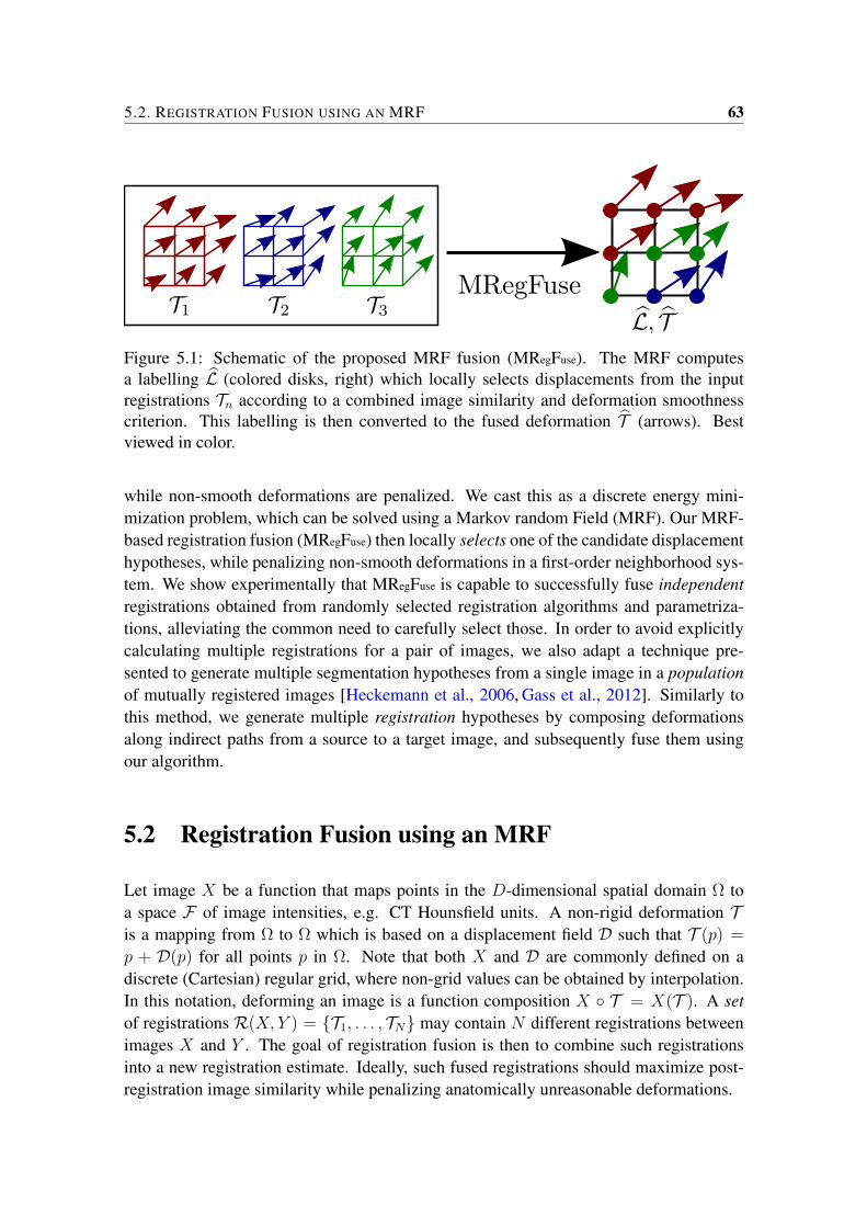
5.2. REGISTRATION FUSION USING AN MRF 63
Figure 5.1: Schematic of the proposed MRF fusion (MRegFuse). The MRF computesa labelling L (colored disks, right) which locally selects displacements from the inputregistrations Tn according to a combined image similarity and deformation smoothnesscriterion. This labelling is then converted to the fused deformation T (arrows). Bestviewed in color.
while non-smooth deformations are penalized. We cast this as a discrete energy mini-mization problem, which can be solved using a Markov random Field (MRF). Our MRF-based registration fusion (MRegFuse) then locally selects one of the candidate displacementhypotheses, while penalizing non-smooth deformations in a first-order neighborhood sys-tem. We show experimentally that MRegFuse is capable to successfully fuse independentregistrations obtained from randomly selected registration algorithms and parametriza-tions, alleviating the common need to carefully select those. In order to avoid explicitlycalculating multiple registrations for a pair of images, we also adapt a technique pre-sented to generate multiple segmentation hypotheses from a single image in a populationof mutually registered images [Heckemann et al., 2006, Gass et al., 2012]. Similarly tothis method, we generate multiple registration hypotheses by composing deformationsalong indirect paths from a source to a target image, and subsequently fuse them usingour algorithm.
5.2 Registration Fusion using an MRF
Let image X be a function that maps points in the D-dimensional spatial domain Ω toa space F of image intensities, e.g. CT Hounsfield units. A non-rigid deformation Tis a mapping from Ω to Ω which is based on a displacement field D such that T (p) =
p + D(p) for all points p in Ω. Note that both X and D are commonly defined on adiscrete (Cartesian) regular grid, where non-grid values can be obtained by interpolation.In this notation, deforming an image is a function composition X T = X(T ). A setof registrations R(X, Y ) = T1, . . . , TN may contain N different registrations betweenimages X and Y . The goal of registration fusion is then to combine such registrationsinto a new registration estimate. Ideally, such fused registrations should maximize post-registration image similarity while penalizing anatomically unreasonable deformations.

64 5. REGISTRATION FUSION USING MARKOV RANDOM FIELDS
We propose a discrete optimization method which locally selects one displacement of Nhypotheses based on local image similarity and global registration smoothness (Fig. 5.1).To this end, we define a discrete label domain L = 1, . . . , N, such that each label luniquely refers to a registration Tl ∈ R(X, Y ). Then, a labelling L : Ω→ L assigns a la-bel lp to every pixel/voxel p of an image. Finally, such labelling defines the correspondingregistration TL as follows:
TL : Ω→ Ω : p→ Tlp(p). (5.1)
This allows us to define the discrete optimization problem as energy minimization ina first-order Markov random field (MRF), for which efficient solvers exist. The MRFenergy is commonly defined as a sum of potential functions defined on a graph whichtypically is the lattice of pixels/voxels in computer vision. The goal of the MRF is thento assign a label lp to each graph node p such that a energy-criterion is minimized. Theenergy that we minimize for our registration fusion problem can then be formalized asfollows:
L = arg minL′
∑p∈Ω
Vp(lp) + λ∑
q∈N (p)
Vpq(lp, lq)
, (5.2)
where the unary term Vp(lp) is the data fitness at point p for label lp, and Vpq is a pairwiseenergy term which allows implementing prior knowledge about the spatial smoothness ofthe solution, and λ is the weighting for the latter.
Unary Term Vp. This term penalizes choosing labels that result in low similarity Φ ofimage X and deformed image Y (Tlp) at location p as follows:
Vp(lp) = 1− Φ(X, Y (Tlp), p
). (5.3)
We use local normalized cross correlation (LNCC) [Cachier et al., 2003] as a robust sim-ilarity metric, which was successfully utilized earlier to locally rank segmentation hy-potheses in [Cardoso et al., 2012]. LNCC is smooth, and can be efficiently computedusing convolutions with Gaussian kernels of size σ. From the LNCC metric, we computethe similarity
Φ(X, Y (Tlp), p
)=
(1 + LNCCσ(X, Y (Tlp), p)
2
)γ, (5.4)
which normalizes LNCC to the range [0, 1]. γ is used to scale the similarity such thatcontributions from individual registrations are well spread [Iglesias and Karssemeijer,2009]. An example of such unary potentials is shown in Fig. 5.2.
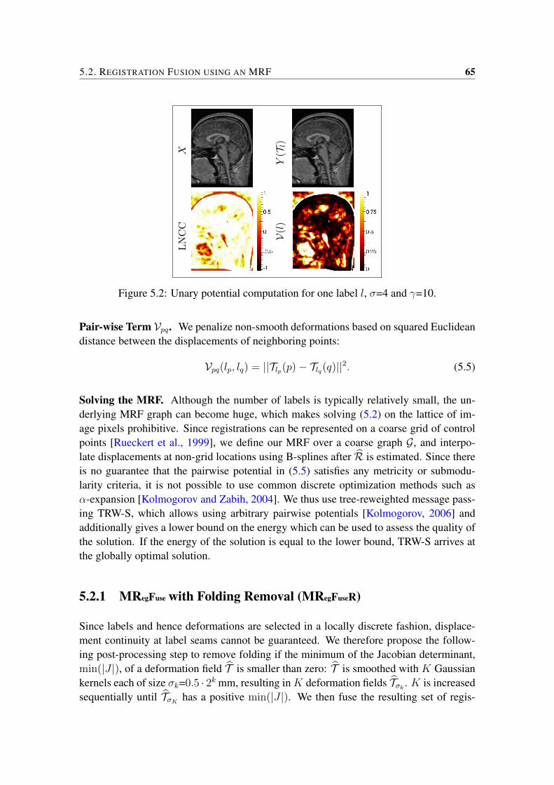
5.2. REGISTRATION FUSION USING AN MRF 65
X
Y(Tl)
LN
CC
V(l)
Figure 5.2: Unary potential computation for one label l, σ=4 and γ=10.
Pair-wise Term Vpq. We penalize non-smooth deformations based on squared Euclideandistance between the displacements of neighboring points:
Vpq(lp, lq) = ||Tlp(p)− Tlq(q)||2. (5.5)
Solving the MRF. Although the number of labels is typically relatively small, the un-derlying MRF graph can become huge, which makes solving (5.2) on the lattice of im-age pixels prohibitive. Since registrations can be represented on a coarse grid of controlpoints [Rueckert et al., 1999], we define our MRF over a coarse graph G, and interpo-late displacements at non-grid locations using B-splines after R is estimated. Since thereis no guarantee that the pairwise potential in (5.5) satisfies any metricity or submodu-larity criteria, it is not possible to use common discrete optimization methods such asα-expansion [Kolmogorov and Zabih, 2004]. We thus use tree-reweighted message pass-ing TRW-S, which allows using arbitrary pairwise potentials [Kolmogorov, 2006] andadditionally gives a lower bound on the energy which can be used to assess the quality ofthe solution. If the energy of the solution is equal to the lower bound, TRW-S arrives atthe globally optimal solution.
5.2.1 MRegFuse with Folding Removal (MRegFuseR)
Since labels and hence deformations are selected in a locally discrete fashion, displace-ment continuity at label seams cannot be guaranteed. We therefore propose the follow-ing post-processing step to remove folding if the minimum of the Jacobian determinant,min(|J |), of a deformation field T is smaller than zero: T is smoothed with K Gaussiankernels each of size σk=0.5 · 2k mm, resulting inK deformation fields Tσk . K is increasedsequentially until TσK has a positive min(|J |). We then fuse the resulting set of regis-
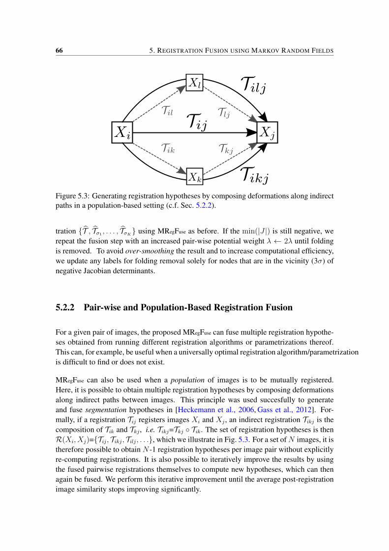
66 5. REGISTRATION FUSION USING MARKOV RANDOM FIELDS
Figure 5.3: Generating registration hypotheses by composing deformations along indirectpaths in a population-based setting (c.f. Sec. 5.2.2).
tration T , Tσ1 , . . . , TσK using MRegFuse as before. If the min(|J |) is still negative, werepeat the fusion step with an increased pair-wise potential weight λ ← 2λ until foldingis removed. To avoid over-smoothing the result and to increase computational efficiency,we update any labels for folding removal solely for nodes that are in the vicinity (3σ) ofnegative Jacobian determinants.
5.2.2 Pair-wise and Population-Based Registration Fusion
For a given pair of images, the proposed MRegFuse can fuse multiple registration hypothe-ses obtained from running different registration algorithms or parametrizations thereof.This can, for example, be useful when a universally optimal registration algorithm/parametrizationis difficult to find or does not exist.
MRegFuse can also be used when a population of images is to be mutually registered.Here, it is possible to obtain multiple registration hypotheses by composing deformationsalong indirect paths between images. This principle was used succesfully to generateand fuse segmentation hypotheses in [Heckemann et al., 2006, Gass et al., 2012]. For-mally, if a registration Tij registers images Xi and Xj , an indirect registration Tikj is thecomposition of Tik and Tkj , i.e. Tikj=Tkj Tik. The set of registration hypotheses is thenR(Xi, Xj)=Tij, Tikj, Tilj, . . ., which we illustrate in Fig. 5.3. For a set ofN images, it istherefore possible to obtain N -1 registration hypotheses per image pair without explicitlyre-computing registrations. It is also possible to iteratively improve the results by usingthe fused pairwise registrations themselves to compute new hypotheses, which can thenagain be fused. We perform this iterative improvement until the average post-registrationimage similarity stops improving significantly.
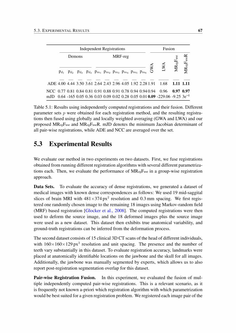
5.3. EXPERIMENTAL RESULTS 67
Independent Registrations Fusion
Demons MRF-reg
GW
A
LWA
MR
egFu
se
MR
egFu
seR
pd1 pd2 pd3 pd4 pm1 pm2 pm3 pm4 pm5 pm6
ADE 4.00 4.44 3.50 3.61 2.64 2.43 2.96 4.05 1.92 2.28 1.91 1.68 1.11 1.11
NCC 0.77 0.81 0.84 0.81 0.91 0.88 0.91 0.78 0.94 0.94 0.94 0.96 0.97 0.97mJD 0.64 -165 0.05 0.36 0.03 0.09 0.02 0.28 0.05 0.01 0.09 -229.06 -9.25 3e-4
Table 5.1: Results using independently computed registrations and their fusion. Differentparameter sets p were obtained for each registration method, and the resulting registra-tions then fused using globally and locally weighted averaging (GWA and LWA) and ourproposed MRegFuse and MRegFuseR. mJD denotes the minimum Jacobian determinant ofall pair-wise registrations, while ADE and NCC are averaged over the set.
5.3 Experimental Results
We evaluate our method in two experiments on two datasets. First, we fuse registrationsobtained from running different registration algorithms with several different parametriza-tions each. Then, we evaluate the performance of MRegFuse in a group-wise registrationapproach.
Data Sets. To evaluate the accuracy of dense registrations, we generated a dataset ofmedical images with known dense correspondences as follows: We used 19 mid-saggitalslices of brain MRI with 481×374 px2 resolution and 0.3 mm spacing. We first regis-tered one randomly chosen image to the remaining 18 images using Markov-random field(MRF) based registration [Glocker et al., 2008]. The computed registrations were thenused to deform the source image, and the 18 deformed images plus the source imagewere used as a new dataset. This dataset then exhibits true anatomical variability, andground-truth registrations can be inferred from the deformation process.
The second dataset consists of 15 clinical 3D CT scans of the head of different individuals,with 160×160×129 px3 resolution and unit spacing. The presence and the number ofteeth vary substantially in this dataset. To evaluate registration accuracy, landmarks wereplaced at anatomically identifiable locations on the jawbone and the skull for all images.Additionally, the jawbone was manually segmented by experts, which allows us to alsoreport post-registration segmentation overlap for this dataset.
Pair-wise Registration Fusion. In this experiment, we evaluated the fusion of mul-tiple independently computed pair-wise registrations. This is a relevant scenario, as itis frequently not known a-priori which registration algorithm with which parametrizationwould be best suited for a given registration problem. We registered each image pair of the
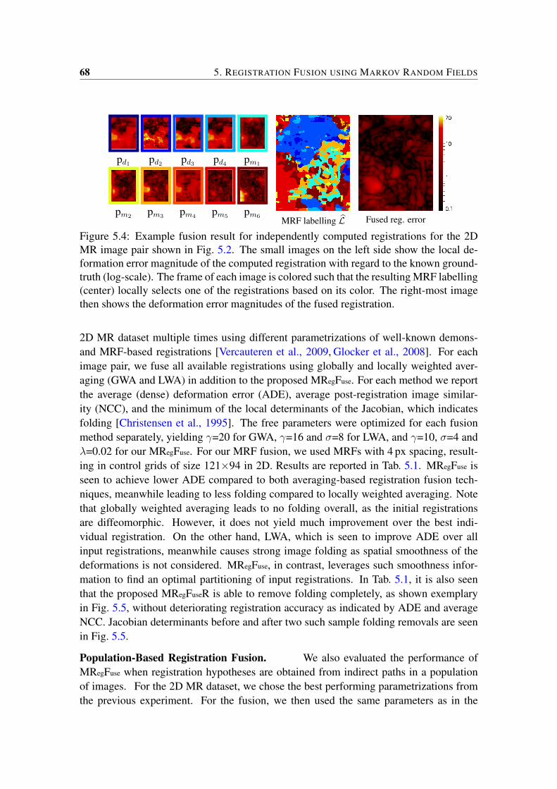
68 5. REGISTRATION FUSION USING MARKOV RANDOM FIELDS
pd1 pd2 pd3 pd4 pm1
pm2 pm3 pm4 pm5 pm6MRF labelling L Fused reg. error
Figure 5.4: Example fusion result for independently computed registrations for the 2DMR image pair shown in Fig. 5.2. The small images on the left side show the local de-formation error magnitude of the computed registration with regard to the known ground-truth (log-scale). The frame of each image is colored such that the resulting MRF labelling(center) locally selects one of the registrations based on its color. The right-most imagethen shows the deformation error magnitudes of the fused registration.
2D MR dataset multiple times using different parametrizations of well-known demons-and MRF-based registrations [Vercauteren et al., 2009, Glocker et al., 2008]. For eachimage pair, we fuse all available registrations using globally and locally weighted aver-aging (GWA and LWA) in addition to the proposed MRegFuse. For each method we reportthe average (dense) deformation error (ADE), average post-registration image similar-ity (NCC), and the minimum of the local determinants of the Jacobian, which indicatesfolding [Christensen et al., 1995]. The free parameters were optimized for each fusionmethod separately, yielding γ=20 for GWA, γ=16 and σ=8 for LWA, and γ=10, σ=4 andλ=0.02 for our MRegFuse. For our MRF fusion, we used MRFs with 4 px spacing, result-ing in control grids of size 121×94 in 2D. Results are reported in Tab. 5.1. MRegFuse isseen to achieve lower ADE compared to both averaging-based registration fusion tech-niques, meanwhile leading to less folding compared to locally weighted averaging. Notethat globally weighted averaging leads to no folding overall, as the initial registrationsare diffeomorphic. However, it does not yield much improvement over the best indi-vidual registration. On the other hand, LWA, which is seen to improve ADE over allinput registrations, meanwhile causes strong image folding as spatial smoothness of thedeformations is not considered. MRegFuse, in contrast, leverages such smoothness infor-mation to find an optimal partitioning of input registrations. In Tab. 5.1, it is also seenthat the proposed MRegFuseR is able to remove folding completely, as shown exemplaryin Fig. 5.5, without deteriorating registration accuracy as indicated by ADE and averageNCC. Jacobian determinants before and after two such sample folding removals are seenin Fig. 5.5.
Population-Based Registration Fusion. We also evaluated the performance ofMRegFuse when registration hypotheses are obtained from indirect paths in a populationof images. For the 2D MR dataset, we chose the best performing parametrizations fromthe previous experiment. For the fusion, we then used the same parameters as in the
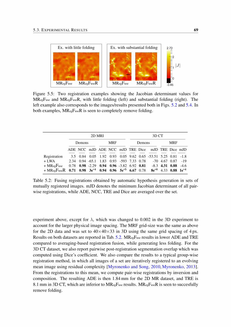
5.3. EXPERIMENTAL RESULTS 69
Ex. with little folding
MRegFuse MRegFuseR
Ex. with substantial folding
MRegFuse MRegFuseR
|J |
Figure 5.5: Two registration examples showing the Jacobian determinant values forMRegFuse and MRegFuseR, with little folding (left) and substantial folding (right). Theleft example also corresponds to the images/results presented both in Figs. 5.2 and 5.4. Inboth examples, MRegFuseR is seen to completely remove folding.
2D MRI 3D CT
Demons MRF Demons MRF
ADE NCC mJD ADE NCC mJD TRE Dice mJD TRE Dice mJD
Registration 3.5 0.84 0.05 1.92 0.93 0.05 9.62 0.65 -53.51 5.25 0.81 -1.8+ LWA 2.34 0.94 -65.1 1.83 0.93 -593 7.33 0.78 -70 4.67 0.87 -19+ MRegFuse 0.78 0.98 -2.29 0.94 0.96 -3.82 6.92 0.81 -8.3 4.31 0.88 -4.6+ MRegFuseR 0.71 0.98 3e-4 0.94 0.96 5e-5 6.67 0.78 8e-6 4.33 0.88 1e-4
Table 5.2: Fusing registrations obtained by automatic hypothesis generation in sets ofmutually registered images. mJD denotes the minimum Jacobian determinant of all pair-wise registrations, while ADE, NCC, TRE and Dice are averaged over the set.
experiment above, except for λ, which was changed to 0.002 in the 3D experiment toaccount for the larger physical image spacing. The MRF grid-size was the same as abovefor the 2D data and was set to 40×40×33 in 3D using the same grid spacing of 4 px.Results on both datasets are reported in Tab. 5.2. MRegFuse results in lower ADE and TREcompared to averaging-based registration fusion, while generating less folding. For the3D CT dataset, we also report pairwise post-registration segmentation overlap which wascomputed using Dice’s coefficient. We also compare the results to a typical group-wiseregistration method, in which all images of a set are iteratively registered to an evolvingmean image using residual complexity [Myronenko and Song, 2010, Myronenko, 2013].From the registrations to this mean, we compute pair-wise registrations by inversion andcomposition. The resulting ADE is then 1.84 mm for the 2D MR dataset, and TRE is8.1 mm in 3D CT, which are inferior to MRegFuse results. MRegFuseR is seen to succesfullyremove folding.
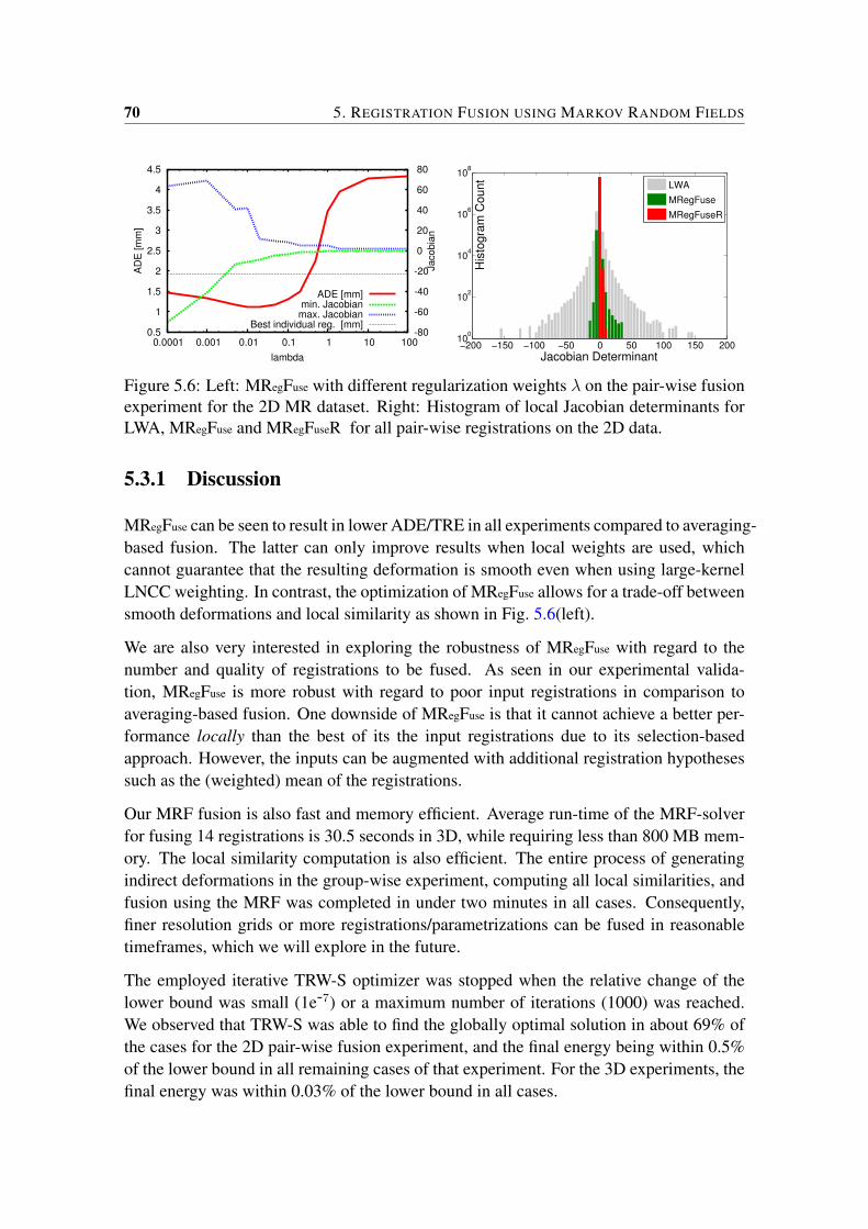
70 5. REGISTRATION FUSION USING MARKOV RANDOM FIELDS
0.5
1
1.5
2
2.5
3
3.5
4
4.5
0.0001 0.001 0.01 0.1 1 10 100-80
-60
-40
-20
0
20
40
60
80
AD
E [
mm
]
Ja
co
bia
n
lambda
ADE [mm]min. Jacobian
max. JacobianBest individual reg. [mm]
−200 −150 −100 −50 0 50 100 150 20010
0
102
104
106
108
Jacobian Determinant
His
togra
m C
ount
LWA
MRegFuse
MRegFuseR
Figure 5.6: Left: MRegFuse with different regularization weights λ on the pair-wise fusionexperiment for the 2D MR dataset. Right: Histogram of local Jacobian determinants forLWA, MRegFuse and MRegFuseR for all pair-wise registrations on the 2D data.
5.3.1 Discussion
MRegFuse can be seen to result in lower ADE/TRE in all experiments compared to averaging-based fusion. The latter can only improve results when local weights are used, whichcannot guarantee that the resulting deformation is smooth even when using large-kernelLNCC weighting. In contrast, the optimization of MRegFuse allows for a trade-off betweensmooth deformations and local similarity as shown in Fig. 5.6(left).
We are also very interested in exploring the robustness of MRegFuse with regard to thenumber and quality of registrations to be fused. As seen in our experimental valida-tion, MRegFuse is more robust with regard to poor input registrations in comparison toaveraging-based fusion. One downside of MRegFuse is that it cannot achieve a better per-formance locally than the best of its the input registrations due to its selection-basedapproach. However, the inputs can be augmented with additional registration hypothesessuch as the (weighted) mean of the registrations.
Our MRF fusion is also fast and memory efficient. Average run-time of the MRF-solverfor fusing 14 registrations is 30.5 seconds in 3D, while requiring less than 800 MB mem-ory. The local similarity computation is also efficient. The entire process of generatingindirect deformations in the group-wise experiment, computing all local similarities, andfusion using the MRF was completed in under two minutes in all cases. Consequently,finer resolution grids or more registrations/parametrizations can be fused in reasonabletimeframes, which we will explore in the future.
The employed iterative TRW-S optimizer was stopped when the relative change of thelower bound was small (1e-7) or a maximum number of iterations (1000) was reached.We observed that TRW-S was able to find the globally optimal solution in about 69% ofthe cases for the 2D pair-wise fusion experiment, and the final energy being within 0.5%of the lower bound in all remaining cases of that experiment. For the 3D experiments, thefinal energy was within 0.03% of the lower bound in all cases.
5.4. CONCLUSIONS 71
As can be seen from the experimental results, the fused registrations still exhibit foldingas indicated by the negative Jacobian determinants. However, both the minima presentedin the tables, as well as the distribution of all such values that can be seen in Fig. 5.6(right)show that the folding is less severe compared to LWA-fusion. Additionally, the proposedMRegFuseR algorithm can be used to remove folding by fusing the original MRegFuse resultwith smoothed versions of itself. This process is seen to retain the high registration ac-curacy of MRegFuse, even with potential (minor) ADE/TRE improvements as seen in thepopulation-based demons experiments in Tab. 5.2. Using the described kernel pyramid,the folding removal in 3D examples needed on average K=4.4 additional smoothed de-formation fields and 12 iterations to remove folding entirely. Since the number of graphlabels during folding removal is significantly smaller compared to the MRegFuse step, therandom field is solved much quicker at 1.5 s on average. The folding removal adds lessthan one minute on average to the registration fusion process. Potentially, such foldingremoval can be applied as a post-processing step to any other registration method thatmay yield non-positive Jacobian determinants.
5.4 Conclusions
We have presented a novel algorithm for registration fusion, which locally selects dis-placements from multiple registration hypotheses. An MRF is used to find an optimalsolution in terms of local post-registration similarity and registration smoothness. Thisalgorithm can furthermore be used to automatically remove inevitable folding at labelseams. The proposed MRegFuse algorithm has been shown to be able to fuse registrationsfrom random parametrizations of different registration algorithms such that the fused reg-istrations exhibit higher accuracy than any of the input registrations. This is a relevantscenario for many image registration applications, where it is typically challenging tochoose and parametrize a registration method correctly. We have also demonstrated thatregistration hypotheses can be obtained automatically within a set of mutually registeredimages, which allows improving the average pair-wise registration accuracy by using theproposed registration fusion.

6Consistency-Based Rectification ofNon-Rigid Registrations
In this paper we present a novel technique to rectify non-rigid registrations by improv-ing their group-wise consistency, which is a widely-used unsupervised measure to assesspair-wise registration quality. While pair-wise registration methods cannot guarantee anygroup-wise consistency, group-wise approaches typically enforce perfect consistency byregistering all images to a common reference. However, errors in individual registrationsto the reference then propagate, distorting the mean and accumulating in the pair-wiseregistrations inferred via the reference. Furthermore, the assumption that perfect cor-respondences exist is not always true, e.g. for inter-patient registration. The proposedconsistency-based registration rectification (CBRR) method addresses these issues byminimizing the group-wise inconsistency of all pair-wise registrations using a regular-ized least-squares algorithm. The regularization controls the adherence to the originalregistration, which is additionally weighted by the local post-registration similarity. Thisallows CBRR to adaptively improve consistency while locally preserving accurate pair-wise registrations. We show that the resulting registrations are not only more consistent,but also have lower average transformation error when compared to known transforma-tions in simulated data. On clinical data, we show improvements of up to 50% TRE inbreathing motion estimation from 4D MRI, and improvements in atlas-based segmenta-tion quality of up to 65% in terms of mean surface distance in 3D CT. Such improvementwas observed consistently using different registration algorithms, dimensionality (2D/3D)and modalities (MRI/CT).
This chapter is currently in review as: Gass, T., Székely, G., and Goksel, O. (2014b). Consistency-Based Rectification of Non-Rigid Registrations. Journal of Medical Imaging, page submitted for review .A preliminary version of this work has been published as: Gass, T., Szekely, G., and Goksel, O. (2014c).Detection and Correction of Inconsistency-based Errors in Non-Rigid Registration. In Proc. SPIE MedicalImaging, volume 9034, page 90341B .
74 6. CONSISTENCY-BASED REGISTRATION RECTIFICATION
6.1 Introduction
Image registration is an essential tool in medical image analysis. It enables applicationssuch as atlas-based segmentation [Rohlfing et al., 2005], statistical model building, andautomatic landmark detection. In many of these tasks, high registration accuracy is criti-cal, but difficult to achieve since the registration problem is known to be ill-posed [Fischerand Modersitzki, 2008] with anatomical correspondences estimated merely using visualsimilarity. Regularization terms based on global smoothness assumptions are commonlyutilized to facilitate anatomically reasonable transformations. However, the resulting elas-tic matching problem is very difficult, and its approximations lead to registration algo-rithms which are only locally optimal. Techniques such as multi-resolution registrationare widely employed to reduce the likelihood of poor local optima [Lee et al., 1997].
There have been several studies that aimed at detecting registration inaccuracies or er-rors posterior to registration. Some of these were based on intensity measures, e.g. usingthe multiple Gaussian state-space [Crum et al., 2004], voxel-statistics based on activeappearance models from registered images [Schestowitz et al., 2006] or supervised learn-ing [Muenzing et al., 2012b, Lotfi et al., 2013]. However, it was shown that such voxelsimilarity metrics are indeed not suitable indicators of registration quality due to homoge-neous tissue regions, partial volume effects, and anatomies of similar appearance [Crumet al., 2003, Rohlfing, 2012]. While independent labelling of landmarks or anatomic re-gions can be used to measure registration fidelity, this requires invaluable time and ef-fort of trained medical personnel, which an automatic registration is supposed to avoidin the first place. To estimate the uncertainty in single pair-wise registrations, differentmethods such as the Cramér-Rao bound [Robinson and Milanfar, 2004], bootstrap re-sampling [Kybic, 2010] or Markov Chain Monte-Carlo (MCMC) [Risholm et al., 2013]have been proposed, often increasing the complexity of a registration algorithm by ordersof magnitude. Recently, such uncertainty estimations have been utilized to improve regis-trations by adaptively estimating an optimal regularization weight [Simpson et al., 2013]or by re-registering uncertain regions in a boosting framework [Muenzing et al., 2012a].
Moving from pairs of images to groups, it is possible to investigate the consistency of mul-tiple registrations as a measure of registration fidelity [Pennec and Thirion, 1997, Woodset al., 1998, Holden et al., 2000, Christensen and Johnson, 2001, Rohlfing, 2012, Datteriand Dawant, 2012]. The most common application of this has been the evaluation andcomparison of registration algorithms by computing the residual norm of inconsistenciesin pair-wise registrations [Woods et al., 1998, Rohlfing, 2012]. Recently, a method wasproposed to exploit redundancy in multiple registration circles for estimating the spatiallocation and magnitude of errors in pair-wise registrations [Datteri and Dawant, 2012].Using a simplified model for the accumulation of registration errors, this method can es-timate a dimensionless measure for local registration error, which was shown therein tocorrelate with true errors. A similar method was also used to predict the segmentation
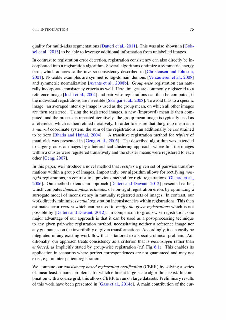
6.1. INTRODUCTION 75
quality for multi-atlas segmentations [Datteri et al., 2011]. This was also shown in [Gok-sel et al., 2013] to be able to leverage additional information from unlabelled images.
In contrast to registration error detection, registration consistency can also directly be in-corporated into a registration algorithm. Several algorithms optimize a symmetric energyterm, which adheres to the inverse consistency described in [Christensen and Johnson,2001]. Noteable examples are symmetric log-domain demons [Vercauteren et al., 2008]and symmetric normalization [Avants et al., 2008b]. Group-wise registration can natu-rally incorporate consistency criteria as well. Here, images are commonly registered to areference image [Joshi et al., 2004] and pair-wise registrations can then be computed, ifthe individual registrations are invertible [Skrinjar et al., 2008]. To avoid bias to a specificimage, an averaged intensity image is used as the group mean, on which all other imagesare then registered. Using the registered images, a new (improved) mean is then com-puted, and the process is repeated iteratively. the group mean image is typically used asa reference, which is then refined iteratively. In order to ensure that the group mean is ina natural coordinate system, the sum of the registrations can additionally be constrainedto be zero [Bhatia and Hajnal, 2004]. A transitive registration method for triplets ofmanifolds was presented in [Geng et al., 2005]. The described algorithm was extendedto larger groups of images by a hierarchical clustering approach, where first the imageswithin a cluster were registered transitively and the cluster means were registered to eachother [Geng, 2007].
In this paper, we introduce a novel method that rectifies a given set of pairwise transfor-mations within a group of images. Importantly, our algorithm allows for rectifying non-rigid registrations, in contrast to a previous method for rigid registrations [Glatard et al.,2006]. Our method extends an approach [Datteri and Dawant, 2012] presented earlier,which computes dimensionless estimates of non-rigid registration errors by optimizing asurrogate model of inconsistency in mutually registered sets of images. In contrast, ourwork directly minimizes actual registration inconsistencies within registrations. This thenestimates error vectors which can be used to rectify the given registrations which is notpossible by [Datteri and Dawant, 2012]. In comparison to group-wise registration, onemajor advantage of our approach is that it can be used as a post-processing techniqueto any given pair-wise registration method, necessitating neither a reference image norany guarantees on the invertibility of given transformations. Accordingly, it can easily beintegrated in any existing work-flow that is tailored to a specific clinical problem. Ad-ditionally, our approach treats consistency as a criterion that is encouraged rather thanenforced, as implicitly stated by group-wise registration (c.f. Fig. 6.1). This enables itsapplication in scenarios where perfect correspondences are not guaranteed and may notexist, e.g. in inter-patient registration.
We compute our consistency based registration rectification (CBRR) by solving a seriesof linear least-squares problems, for which efficient large-scale algorithms exist. In com-bination with a coarse grid, this allows CBRR to run on large datasets. Preliminary resultsof this work have been presented in [Gass et al., 2014c]. A main contribution of the cur-
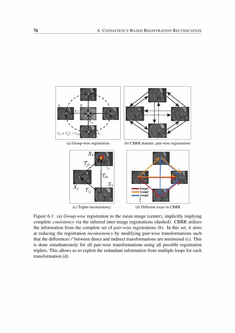
76 6. CONSISTENCY-BASED REGISTRATION RECTIFICATION
(a) Group-wise registration (b) CBRR domain: pair-wise registrations
(c) Triplet inconsistency (d) Different loops in CBRR
Figure 6.1: (a) Group-wise registration to the mean image (center), implicitly implyingcomplete consistency via the inferred inter-image registrations (dashed). CBRR utilisesthe information from the complete set of pair-wise registrations (b). In this set, it aimsat reducing the registration inconsistency by modifying pair-wise transformations suchthat the differences ~r between direct and indirect transformations are minimised (c). Thisis done simultaneously for all pair-wise transformations using all possible registrationtriplets. This allows us to exploit the redundant information from multiple loops for eachtransformation (d).
6.2. NOTATION AND BACKGROUND 77
rent paper is an improved formulation of the CBRR problem which (i) requires only halfof the free variables compared to [Gass et al., 2014c]; (ii) requires fewer weighting pa-rameters; and (iii) allows for an iterative rectification process yielding better accuracy foremployed approximations and thereby improving the resulting registrations. We presenta thorough evaluation of CBRR on fully synthetic and clinical data. Consistency is shownto improve on datasets of 2D and 3D images, while average transformation error, targetregistration error, and segmentation overlap improve substantially, regardless of initialregistration algorithm and image modality. Such measures are also shown to outperforma common group-wise registration algorithm.
This paper is structured as follows: First, we introduce the notation used in this paper,along with a presentation of common concepts regarding consistency. Subsequently, wedescribe our CBRR algorithm before presenting experimental results and a discussionthereof.
6.2 Notation and Background
An image X is a function that maps points in the D-dimensional spatial domain Ω toa space I of image intensities, e.g. CT Hounsfield units. A non-rigid transformationT is a mapping from Ω to Ω. T is based on a displacement field D such that T (p) =
p+D(p) for all points p in Ω. Note that both X and D are commonly defined on discrete(Cartesian) regular grids, where non-grid values can be obtained by interpolation. In thisnotation, deforming an image is a function composition X T = X(T ). Composing twotransformations is also a function composition: (T2 T1) (p) = p + D1(p) + D2(T1(p)). denotes the composition operator, read from right to left. Therefore, T2 T1 meanstransformation T2 applied after T1.
Several studies [Rohlfing, 2012, Woods et al., 1998, Holden et al., 2000, Christensen andJohnson, 2001] have presented methods for estimating registration accuracy using theconsistency of a pairwise transformation set (PTS):
R = Tij|i 6= j; i, j ∈ 1, · · · , N
between images of a set X = X1, · · · , XN. Tij then denotes the transformation ofimage Xi to Xj . As originally introduced in [Woods et al., 1998], a perfect registra-tion should lead to consistent correspondences over the entire set of images. Inverseconsistency as given in [Rohlfing, 2012, Christensen and Johnson, 2001] stipulates thatregistering Xi to Xj should result in the same transformation as the inversion of the trans-formation from registering Xj to Xi. Formally, it requires Tij Tji = I, where I is theidentity transform. Another form of consistency is based on registration circuits [Holden
78 6. CONSISTENCY-BASED REGISTRATION RECTIFICATION
et al., 2000], where any composition of transformations in a circle should result in theidentity transform; for instance, for a circle of three transformations:
Tij Tjk Tki = I. (6.1)
Transitivity has also been used for consistency evaluation [Christensen and Johnson, 2003].Intuitively, transitivity entails that composing two transformations from registering Xi toXj and Xj to Xk should result in the same transformation as registering Xi to Xk:
Tik = Tij Tjk. (6.2)
Note that transitivity and circuit consistency follow from each other when the transforma-tions are symmetric. A general definition of consistency is the following: Let Φn
ij be theset of all paths of length n such that each path p ∈ Φn
ij is a composition of n transforma-tions T1, T2, · · · , Tn that registers Xi to Xj . Then, the PTS R is (m,n)-consistent iffp = q for all transformations p ∈ Φm
ij and q ∈ Φnij . In this notation, inverse consistency
can be denoted as (2, 0)-consistency, circuit consistency as (3, 0)-consistency for circuitsof length 3 and transitivity as (2, 1)-consistency. Since each pair p and q share the samestart and end points, we will henceforth refer to each such pair as a loop. Then, the in-consistency can be quantified using the residual vector fields rpq = p− q for p ∈ Φm
ij andq ∈ Φn
ij . In this notation the metric for algorithmic efficacy of a transformation can becomputed as the mean over the norms of all rpq [Song et al., 2010].
6.3 Method
In this section, we introduce our algorithm for Consistency-Based Registration Rectifica-tion (CBRR). The goal of the method is to improve pair-wise registrations by minimisingan inconsistency criterion C defined as the average norm of the inconsistency residuals r.Note that consistency is only a necessary condition for correct registrations. This can in-tuitively be observed when considering the set of identity transforms, which are perfectlyconsistent but are unlikely to register images properly. This effect can also partly be seenin Fig. 6.2, where several loops with low inconsistency but substantial registration errorscan be observed. We therefore additionally constrain the solution of CBRR by penalizinglarge deviations from the input PTS R using a function F . This then makes use of thefact that a prior PTSR contains useful information.
We define our CBRR algorithm as the minimisation of the inconsistency criterion C for agiven input PTSR obtained using an arbitrary registration method as follows:
R′ = arg minRC(R) + λF(R, R), (6.3)

6.3. METHOD 79
0
1
2
3
4
5
6
7
8
0 2 4 6 8 10 12 14
avg
. T
RE
[m
m]
Inconsistency [mm]
r=0.77
Registration algorithm ARegistration algorithm B
Figure 6.2: Inconsistency and target registration error (TRE) for registration loops in4D liver MRI sequences. Each point indicates the inconsistency of one loop of threeregistrations and the average TRE of those three registrations, and the blue line is a least-square fit with r=0.77 denoting the Pearson correlation. For more details on the data andregistration algorithms please see Sec. 6.4.4.
where R′ is the rectified PTS and λ is the weight controlling its adherence to the priortransformations.
6.3.1 CBRR Algorithm: Consistency
CBRR minimises the aggregate inconsistency that is induced by all loops in the set ofpair-wise transformations:
C(R) =N∑i=1
N∑j=1j 6=i
∑p∈Φm
ij
∑q∈Φn
ij
||p− q||2 . (6.4)
A desireable property of such inconsistency criterion is redundancy, which means thateach pair-wise registration occurs in the residual of multiple loops. This is an importantcue for determining the cause of inconsistencies in a registration. For example, considera PTS R where only one transformation Tij has errors which cause inconsistencies. Anyconsistency loop containing Tij will therefore have a non-negative residual r, the cause ofwhich cannot easily be located using only information from said loops alone. However,since every transformation other than Tij will also contribute to multiple loops that all havezero residuals, it is thus inferable that the cause of inconsistency originates from Tij . It isobservable that such redundancy is created for any m and n when m + n > 2. However,the number of summands in (6.4) increases exponentially with m and n. Furthermore,each transformation composition, especially in longer paths, will require interpolationand therefore loses accuracy. This motivates our choice of consistency criterion as (2, 1)-
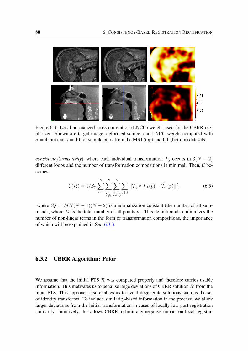
80 6. CONSISTENCY-BASED REGISTRATION RECTIFICATION
Figure 6.3: Local normalized cross correlation (LNCC) weight used for the CBRR reg-ularizer. Shown are target image, deformed source, and LNCC weight computed withσ = 4 mm and γ = 10 for sample pairs from the MRI (top) and CT (bottom) datasets.
consistency(transitivity), where each individual transformation Tij occurs in 3(N − 2)
different loops and the number of transformation compositions is minimal. Then, C be-comes:
C(R) = 1/ZC
N∑i=1
N∑j=1j 6=i
N∑k=1k 6=i,j
∑p∈Ω
||Tij Tjk(p)− Tik(p)||2, (6.5)
where ZC = MN(N − 1)(N − 2) is a normalization constant (the number of all sum-mands, where M is the total number of all points p). This definition also minimizes thenumber of non-linear terms in the form of transformation compositions, the importanceof which will be explained in Sec. 6.3.3.
6.3.2 CBRR Algorithm: Prior
We assume that the initial PTS R was computed properly and therefore carries usableinformation. This motivates us to penalise large deviations of CBRR solution R′ from theinput PTS. This approach also enables us to avoid degenerate solutions such as the setof identity transforms. To include similarity-based information in the process, we allowlarger deviations from the initial transformation in cases of locally low post-registrationsimilarity. Intuitively, this allows CBRR to limit any negative impact on local registra-

6.3. METHOD 81
tion accuracy while improving consistency. We then define such penalty function F asfollows:
F(R,R) = 1/ZF
N∑i=1
N∑j=1j 6=i
∑p∈Ω
Ψij(p)||Tij(p)− Tij(p)||2, (6.6)
where p ∈ Ω is a (discrete) point, ZF = MN(N − 1) is a normalization constant, andΨij is the local similarity between the transformed image Xi(Tij) and Xj .
We use local normalized cross correlation (LNCC) [Cachier et al., 2003] as the localsimilarity metric, which was successfully utilized to locally rank segmentation hypothesesin [Cardoso et al., 2012]. LNCC can be computed efficiently as follows:
LNCC(Xi, Xj, p) =〈Xi, Xj〉(p)σXi
(p) σXj(p)
(6.7)
〈Xi, Xj〉(p) = Xi ·Xj(p)−Xi(p) ·Xj(p) (6.8)
X = GσG ∗X (6.9)
σ2Xi
(p) = Xi2(p)−Xi
2(p), (6.10)
where ∗ is the convolution operator and GσG is a Gaussian kernel with standard deviationσG . From the LNCC metric, we compute the weights
Ψij =
(1.0− LNCC(Xi(Tij), Xj)
2
)γ, (6.11)
which normalizes LNCC to the range [0, 1] and subsequently applies a contrast scalingusing γ. The resulting local weights are shown on an example in Fig. 6.3.
6.3.3 Casting into a System of Linear Equations
We find a solution for (6.3) by casting it as a linear least-squares optimization problem,for which efficient large-scale algorithms exist. The only non-linear term is the transfor-mation composition in (6.5), which we approximate as follows:
Tij Tjk − Tik = Dij(Tjk) + Djk − Dik (6.12)
≈ Dij(Tjk) + Djk − Dik, (6.13)
by substituting the unknown true transformation Tjk in (6.12) with the observed transfor-mation Tjk when it is used to deform the displacement field Dij .

82 6. CONSISTENCY-BASED REGISTRATION RECTIFICATION
This allows us to rewrite the minimization problem in the form of x′ = minx|Ax − b|2,
where x is the column vector of all grid-point displacement variables for all transforma-tions in R. Then, x has MN(N − 1) entries and has the form
x =[D1,2(p1), · · · , Dij(pm), · · · , DN−1,N(pM)
]T(6.14)
The matrix A and the vector b can be decomposed into two parts, AC and bC for theconsistency criterion and AF and bF for the regularization term:
x′ = minx
∣∣∣∣[ACAF]
x−[bCbF
]∣∣∣∣2 . (6.15)
Each row of AC consists of 0s and ±1s such that multiplication with x yields one of thesummands of the consistency criterion. The locations of the nonzero entries correspond tothe locations of the respective displacements in the vector x and can be calculated with thehelp of an indexing function idx that returns the index of displacement p in transformationTij as follows:
idx : N3 → N : idx(i, j, p)→ 1, . . . ,MN(N − 1) (6.16)
Then, each row r ofAc corresponding to a consistency term Dij(Tjk(p))+Djk(p)−Dik(p)has the following entries in columns c:
AC(r, c) =
1 , if c = idx(i, j, Tjk(p)) or c = idx(j, k, (p))
−1 , if c = idx(i, k, p)
0 , otherwise.
(6.17)
All corresponding entries in bC are then zero, since we want the inconsistency to vanish.When Tjk(p) is not on a grid point, we use linear interpolation:
Dij(Tjk(p)) + Djk(p)− Dik(p) ≈
∑p′∈N (Tjk(p))
ν(p′) · Dij(p′)
+ Djk(p)− Dik(p),
(6.18)
where N returns the grid neighborhood of a non-grid point, and ν computes the inter-polation weights. Thus, such consistency-expressing rows in AC can contain up to 10non-zero elements in 3D, where the first non-grid point is interpolated from 8 neighbor-ing grid points.
AF is a square, diagonal matrix such that the multiplication of one row of AF with x andsubtracting the corresponding entry of bF yields one of the prior terms λΨij(p)Dij(p) −λΨij(p)Dij(p) being minimized. In the same notation as above, this can be expressed as:
6.3. METHOD 83
AF(r, c) =
λΨij(p) , if r = c
0 , otherwise.(6.19)
bF(c) = λΨij(p)Dij(p) (6.20)
with c = idx(i, j, p). (6.21)
6.3.4 Iterative Refinement
In order to improve the approximation in (6.13), we employ a fixed point iterative updatescheme. In each iteration t, a new PTS Rt is computed, where R0 is the CBRR initial-isation from a prior registration. The estimate of the last iteration is then used for theapproximation in (6.13) as follows:
T tij T tjk − T tik ≈ Dtij(T t−1jk ) +Dtjk −Dtik. (6.22)
This allows the approximation to become more accurate as the difference between T t−1
and T t becomes smaller. The iterative process can also be used to update the priorterm. Since we assume that the input registration contains errors, adhering too stronglyto it might deteriorate the results of the algorithm. A straight-forward way to check forimprovements during the iterations is to compare the local post-registration similarities.We therefore re-compute the local similarity weights Ψt after every iteration, and keeptrack of the locally best encountered value along with the corresponding displacement:
(Ψbest,Dbest)ijp =
(Ψt,Dt)ijp , if Ψt
ij(p) > Ψbestij (p)
(Ψbest,Dbest)ijp , otherwise,(6.23)
where we moved the sub-indices outside of the tuples for readability. Then, we changethe prior terms in (6.6) to penalize differences from these current best estimates:
F(R,Rbest) = 1/ZF
N∑i=1
N∑j=1j 6=i
∑p∈Ω
Ψbestij (p)||Dij(p)−Dbest
ij (p)||2. (6.24)
6.3.5 Implementation
The number of equations grows with the cube of the number of images, N , and linearlywith the number of pixels, M . However, efficient algorithms for solving large-scale linear
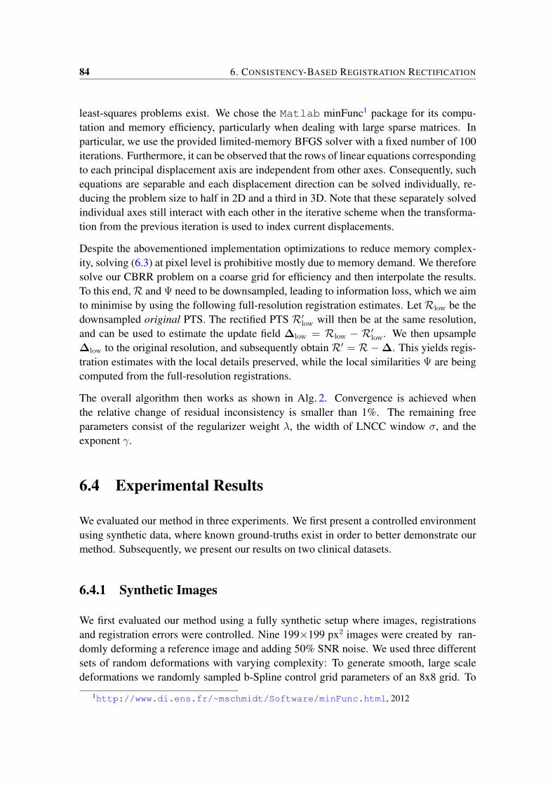
84 6. CONSISTENCY-BASED REGISTRATION RECTIFICATION
least-squares problems exist. We chose the Matlab minFunc1 package for its compu-tation and memory efficiency, particularly when dealing with large sparse matrices. Inparticular, we use the provided limited-memory BFGS solver with a fixed number of 100iterations. Furthermore, it can be observed that the rows of linear equations correspondingto each principal displacement axis are independent from other axes. Consequently, suchequations are separable and each displacement direction can be solved individually, re-ducing the problem size to half in 2D and a third in 3D. Note that these separately solvedindividual axes still interact with each other in the iterative scheme when the transforma-tion from the previous iteration is used to index current displacements.
Despite the abovementioned implementation optimizations to reduce memory complex-ity, solving (6.3) at pixel level is prohibitive mostly due to memory demand. We thereforesolve our CBRR problem on a coarse grid for efficiency and then interpolate the results.To this end,R and Ψ need to be downsampled, leading to information loss, which we aimto minimise by using the following full-resolution registration estimates. Let Rlow be thedownsampled original PTS. The rectified PTS R′low will then be at the same resolution,and can be used to estimate the update field ∆low = Rlow − R′low. We then upsample∆low to the original resolution, and subsequently obtain R′ = R−∆. This yields regis-tration estimates with the local details preserved, while the local similarities Ψ are beingcomputed from the full-resolution registrations.
The overall algorithm then works as shown in Alg. 2. Convergence is achieved whenthe relative change of residual inconsistency is smaller than 1%. The remaining freeparameters consist of the regularizer weight λ, the width of LNCC window σ, and theexponent γ.
6.4 Experimental Results
We evaluated our method in three experiments. We first present a controlled environmentusing synthetic data, where known ground-truths exist in order to better demonstrate ourmethod. Subsequently, we present our results on two clinical datasets.
6.4.1 Synthetic Images
We first evaluated our method using a fully synthetic setup where images, registrationsand registration errors were controlled. Nine 199×199 px2 images were created by ran-domly deforming a reference image and adding 50% SNR noise. We used three differentsets of random deformations with varying complexity: To generate smooth, large scaledeformations we randomly sampled b-Spline control grid parameters of an 8x8 grid. To
1http://www.di.ens.fr/~mschmidt/Software/minFunc.html, 2012
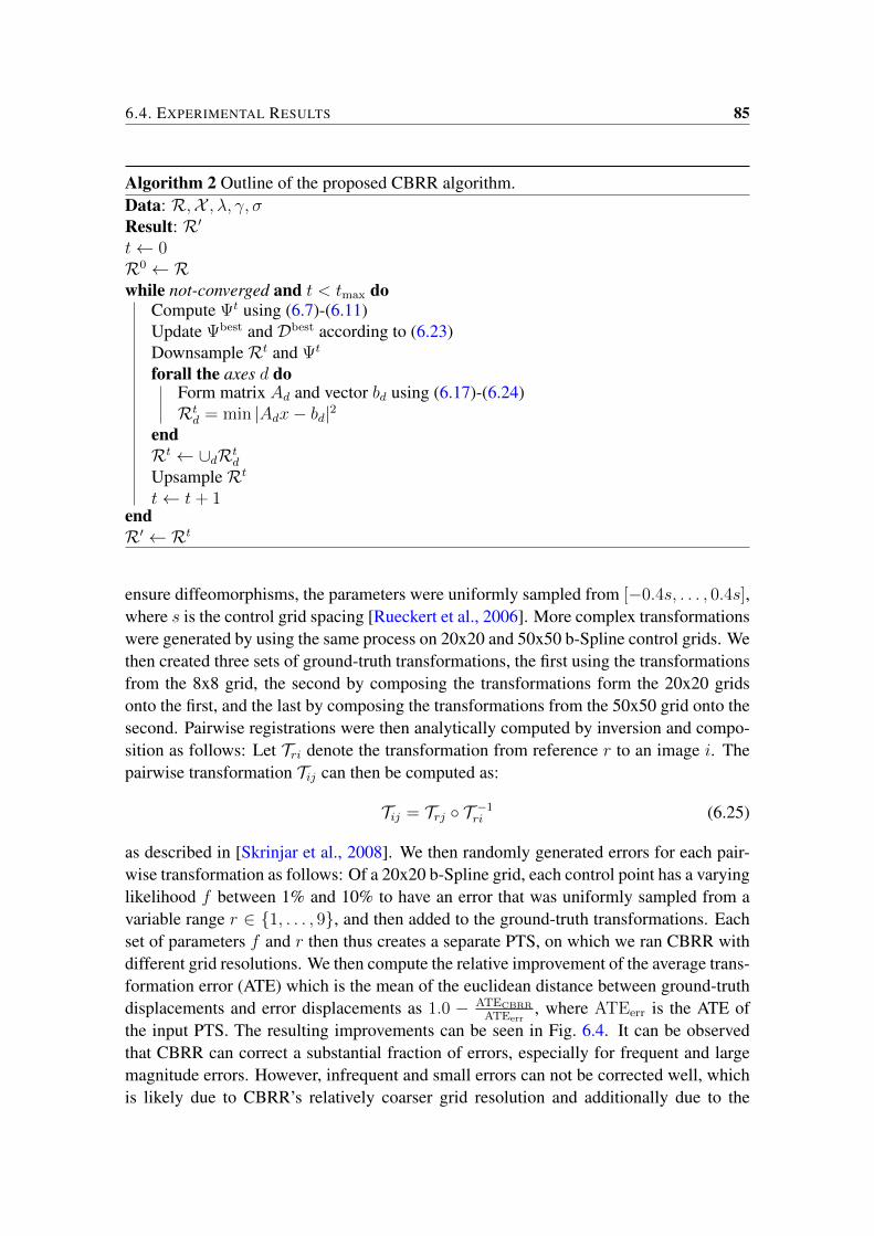
6.4. EXPERIMENTAL RESULTS 85
Algorithm 2 Outline of the proposed CBRR algorithm.Data: R,X , λ, γ, σResult: R′t← 0R0 ← Rwhile not-converged and t < tmax do
Compute Ψt using (6.7)-(6.11)Update Ψbest and Dbest according to (6.23)DownsampleRt and Ψt
forall the axes d doForm matrix Ad and vector bd using (6.17)-(6.24)Rtd = min |Adx− bd|2
endRt ← ∪dRt
d
UpsampleRt
t← t+ 1endR′ ← Rt
ensure diffeomorphisms, the parameters were uniformly sampled from [−0.4s, . . . , 0.4s],where s is the control grid spacing [Rueckert et al., 2006]. More complex transformationswere generated by using the same process on 20x20 and 50x50 b-Spline control grids. Wethen created three sets of ground-truth transformations, the first using the transformationsfrom the 8x8 grid, the second by composing the transformations form the 20x20 gridsonto the first, and the last by composing the transformations from the 50x50 grid onto thesecond. Pairwise registrations were then analytically computed by inversion and compo-sition as follows: Let Tri denote the transformation from reference r to an image i. Thepairwise transformation Tij can then be computed as:
Tij = Trj T −1ri (6.25)
as described in [Skrinjar et al., 2008]. We then randomly generated errors for each pair-wise transformation as follows: Of a 20x20 b-Spline grid, each control point has a varyinglikelihood f between 1% and 10% to have an error that was uniformly sampled from avariable range r ∈ 1, . . . , 9, and then added to the ground-truth transformations. Eachset of parameters f and r then thus creates a separate PTS, on which we ran CBRR withdifferent grid resolutions. We then compute the relative improvement of the average trans-formation error (ATE) which is the mean of the euclidean distance between ground-truthdisplacements and error displacements as 1.0 − ATECBRR
ATEerr, where ATEerr is the ATE of
the input PTS. The resulting improvements can be seen in Fig. 6.4. It can be observedthat CBRR can correct a substantial fraction of errors, especially for frequent and largemagnitude errors. However, infrequent and small errors can not be corrected well, whichis likely due to CBRR’s relatively coarser grid resolution and additionally due to the
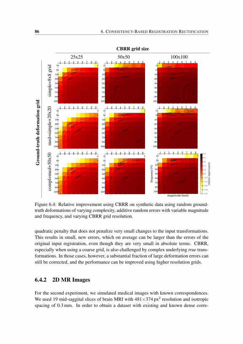
86 6. CONSISTENCY-BASED REGISTRATION RECTIFICATION
CBRR grid size
25x25 50x50 100x100
Gro
und-
trut
hde
form
atio
ngr
id
sim
ple=
8x8
grid
1 2 3 4 5 6 7 8 9
magnitude [mm]
1
5
10
20
30
50
70
90
100
freq
uenc
y[%
]
0.000
0.200
0.400
−1.0
−0.8
−0.6
−0.4
−0.2
0.0
0.2
0.4
0.6
0.8
1.0
rela
tive
impr
ovem
ent
1 2 3 4 5 6 7 8 9
magnitude [mm]
1
5
10
20
30
50
70
90
100fr
eque
ncy
[%]
0.000 0.2000.400
0.600
0.650
−1.0
−0.8
−0.6
−0.4
−0.2
0.0
0.2
0.4
0.6
0.8
1.0
rela
tive
impr
ovem
ent
1 2 3 4 5 6 7 8 9
magnitude [mm]
1
5
10
20
30
50
70
90
100
freq
uenc
y[%
]
0.200 0.400
0.600
0.650
0.700
0.700
0.700
−1.0
−0.8
−0.6
−0.4
−0.2
0.0
0.2
0.4
0.6
0.8
1.0
rela
tive
impr
ovem
ent
med
=sim
ple+
20x2
0 1 2 3 4 5 6 7 8 9
magnitude [mm]
1
5
10
20
30
50
70
90
100
freq
uenc
y[%
]
0.000
0.200
0.400
−1.0
−0.8
−0.6
−0.4
−0.2
0.0
0.2
0.4
0.6
0.8
1.0re
lati
veim
prov
emen
t1 2 3 4 5 6 7 8 9
magnitude [mm]
1
5
10
20
30
50
70
90
100
freq
uenc
y[%
]
0.0000.200
0.400
0.600
0.650
−1.0
−0.8
−0.6
−0.4
−0.2
0.0
0.2
0.4
0.6
0.8
1.0
rela
tive
impr
ovem
ent
1 2 3 4 5 6 7 8 9
magnitude [mm]
1
5
10
20
30
50
70
90
100
freq
uenc
y[%
]
0.0000.000
0.2000.400
0.600
0.650
−1.0
−0.8
−0.6
−0.4
−0.2
0.0
0.2
0.4
0.6
0.8
1.0
rela
tive
impr
ovem
ent
com
pl=m
ed+5
0x50
1 2 3 4 5 6 7 8 9
magnitude [mm]
1
5
10
20
30
50
70
90
100
freq
uenc
y[%
]
0.000
0.200
0.400
−1.0
−0.8
−0.6
−0.4
−0.2
0.0
0.2
0.4
0.6
0.8
1.0
rela
tive
impr
ovem
ent
1 2 3 4 5 6 7 8 9
magnitude [mm]
1
5
10
20
30
50
70
90
100
freq
uenc
y[%
]
0.0000.200
0.400
0.600
−1.0
−0.8
−0.6
−0.4
−0.2
0.0
0.2
0.4
0.6
0.8
1.0re
lati
veim
prov
emen
t1 2 3 4 5 6 7 8 9
magnitude [mm]
1
5
10
20
30
50
70
90
100
freq
uenc
y[%
]
0.0000.200
0.400
0.600
0.650
−1.0
−0.8
−0.6
−0.4
−0.2
0.0
0.2
0.4
0.6
0.8
1.0
rela
tive
impr
ovem
ent
Figure 6.4: Relative improvement using CBRR on synthetic data using random ground-truth deformations of varying complexity, additive random errors with variable magnitudeand frequency, and varying CBRR grid resolution.
quadratic penalty that does not penalize very small changes to the input transformations.This results in small, new errors, which on average can be larger than the errors of theoriginal input registration, even though they are very small in absolute terms. CBRR,especially when using a coarse grid, is also challenged by complex underlying true trans-formations. In those cases, however, a substantial fraction of large deformation errors canstill be corrected, and the performance can be improved using higher resolution grids.
6.4.2 2D MR Images
For the second experiment, we simulated medical images with known correspondences.We used 19 mid-saggital slices of brain MRI with 481×374 px2 resolution and isotropicspacing of 0.3 mm. In order to obtain a dataset with existing and known dense corre-
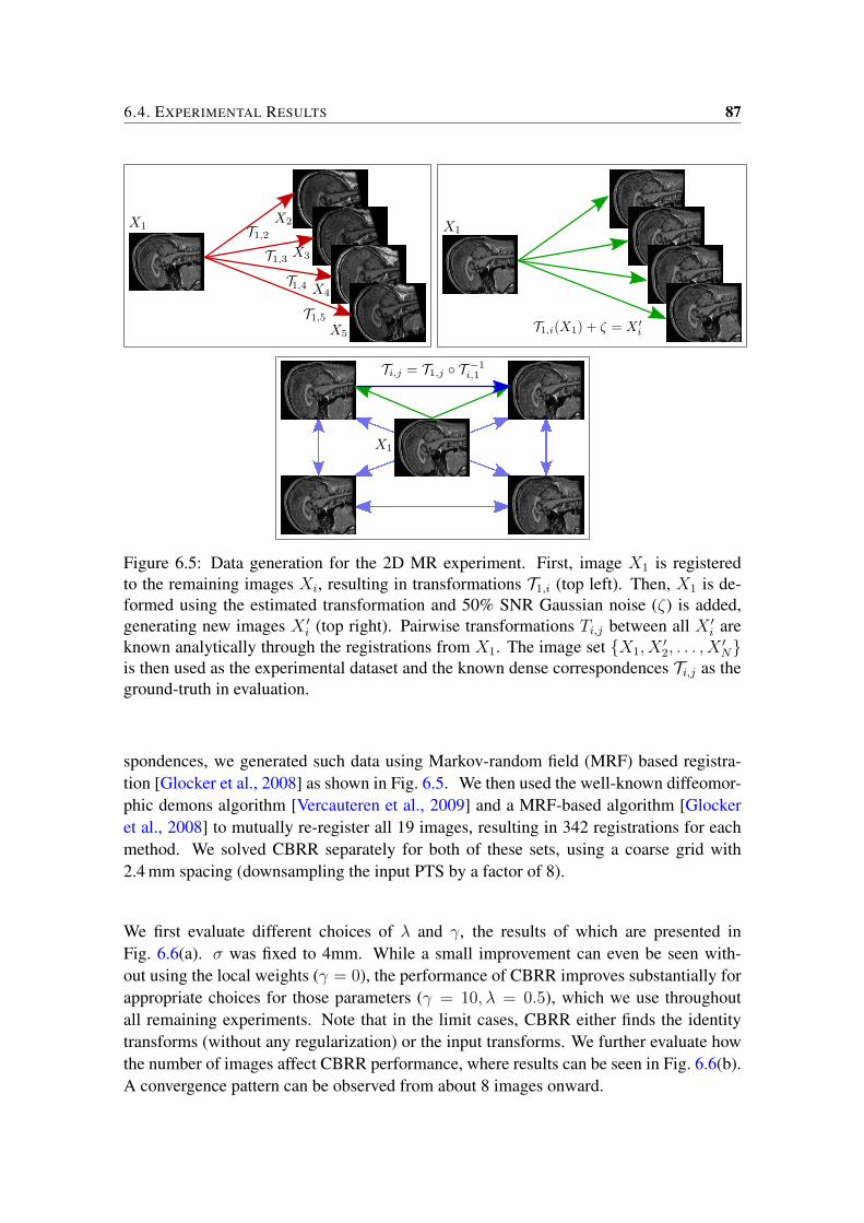
6.4. EXPERIMENTAL RESULTS 87
Figure 6.5: Data generation for the 2D MR experiment. First, image X1 is registeredto the remaining images Xi, resulting in transformations T1,i (top left). Then, X1 is de-formed using the estimated transformation and 50% SNR Gaussian noise (ζ) is added,generating new images X ′i (top right). Pairwise transformations Ti,j between all X ′i areknown analytically through the registrations from X1. The image set X1, X
′2, . . . , X
′N
is then used as the experimental dataset and the known dense correspondences Ti,j as theground-truth in evaluation.
spondences, we generated such data using Markov-random field (MRF) based registra-tion [Glocker et al., 2008] as shown in Fig. 6.5. We then used the well-known diffeomor-phic demons algorithm [Vercauteren et al., 2009] and a MRF-based algorithm [Glockeret al., 2008] to mutually re-register all 19 images, resulting in 342 registrations for eachmethod. We solved CBRR separately for both of these sets, using a coarse grid with2.4 mm spacing (downsampling the input PTS by a factor of 8).
We first evaluate different choices of λ and γ, the results of which are presented inFig. 6.6(a). σ was fixed to 4mm. While a small improvement can even be seen with-out using the local weights (γ = 0), the performance of CBRR improves substantially forappropriate choices for those parameters (γ = 10, λ = 0.5), which we use throughoutall remaining experiments. Note that in the limit cases, CBRR either finds the identitytransforms (without any regularization) or the input transforms. We further evaluate howthe number of images affect CBRR performance, where results can be seen in Fig. 6.6(b).A convergence pattern can be observed from about 8 images onward.
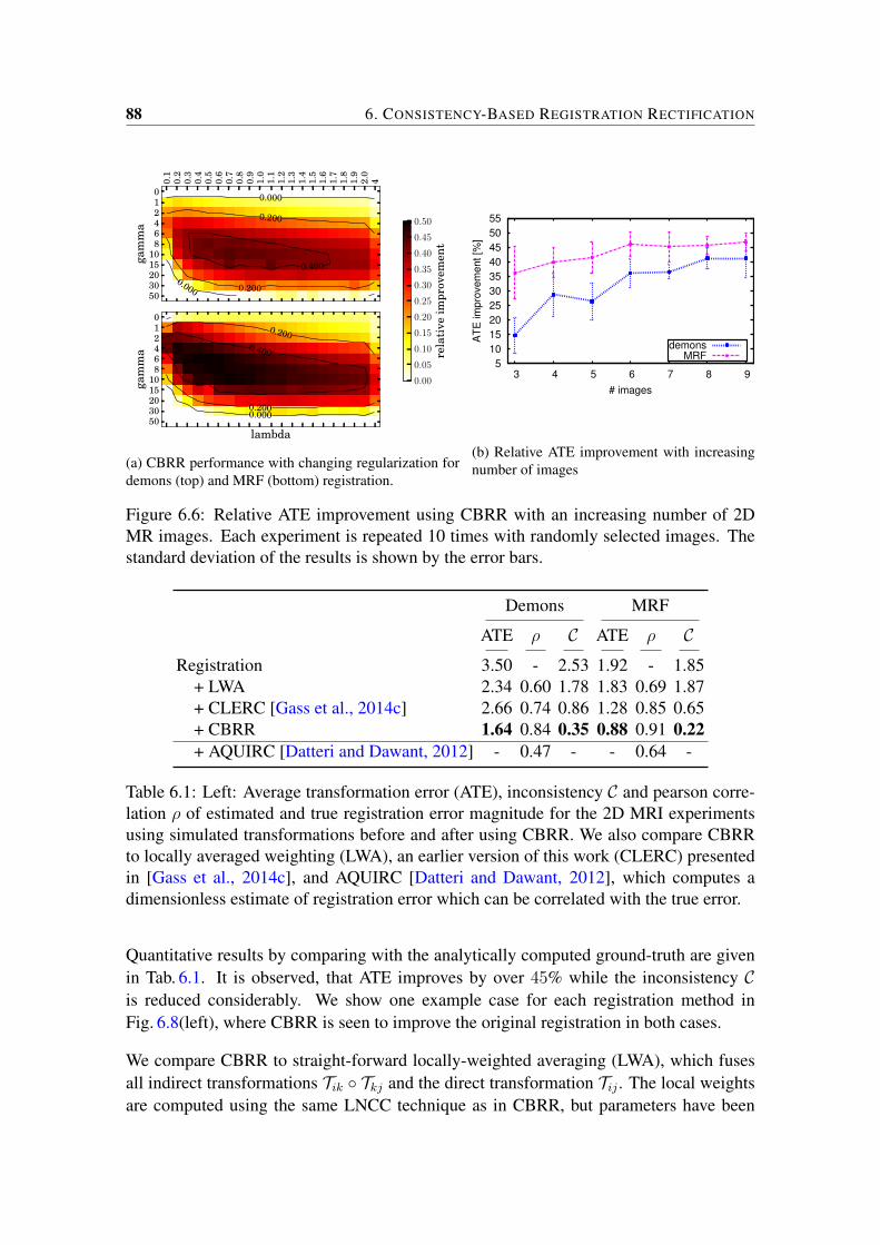
88 6. CONSISTENCY-BASED REGISTRATION RECTIFICATION
0.1
0.2
0.3
0.4
0.5
0.6
0.7
0.8
0.9
1.0
1.1
1.2
1.3
1.4
1.5
1.6
1.7
1.8
1.9
2.0
4
lambda
012468
1015203050
gam
ma
0.000
0.000
0.200
0.200
0.400
0.00
0.05
0.10
0.15
0.20
0.25
0.30
0.35
0.40
0.45
0.50
rela
tive
impr
ovem
ent
0.1
0.2
0.3
0.4
0.5
0.6
0.7
0.8
0.9
1.0
1.1
1.2
1.3
1.4
1.5
1.6
1.7
1.8
1.9
2.0
4lambda
012468
1015203050
gam
ma
0.000
0.000
0.200
0.200
0.400
0.00
0.05
0.10
0.15
0.20
0.25
0.30
0.35
0.40
0.45
0.50
rela
tive
impr
ovem
ent
0.1
0.2
0.3
0.4
0.5
0.6
0.7
0.8
0.9
1.0
1.1
1.2
1.3
1.4
1.5
1.6
1.7
1.8
1.9
2.0
4
lambda
012468
1015203050
gam
ma
0.000
0.200
0.200
0.400
0.00
0.05
0.10
0.15
0.20
0.25
0.30
0.35
0.40
0.45
0.50
rela
tive
impr
ovem
ent
(a) CBRR performance with changing regularization fordemons (top) and MRF (bottom) registration.
5
10
15
20
25
30
35
40
45
50
55
3 4 5 6 7 8 9
AT
E im
pro
vem
ent [%
]
# images
demonsMRF
(b) Relative ATE improvement with increasingnumber of images
Figure 6.6: Relative ATE improvement using CBRR with an increasing number of 2DMR images. Each experiment is repeated 10 times with randomly selected images. Thestandard deviation of the results is shown by the error bars.
Demons MRF
ATE ρ C ATE ρ CRegistration 3.50 - 2.53 1.92 - 1.85
+ LWA 2.34 0.60 1.78 1.83 0.69 1.87+ CLERC [Gass et al., 2014c] 2.66 0.74 0.86 1.28 0.85 0.65+ CBRR 1.64 0.84 0.35 0.88 0.91 0.22+ AQUIRC [Datteri and Dawant, 2012] - 0.47 - - 0.64 -
Table 6.1: Left: Average transformation error (ATE), inconsistency C and pearson corre-lation ρ of estimated and true registration error magnitude for the 2D MRI experimentsusing simulated transformations before and after using CBRR. We also compare CBRRto locally averaged weighting (LWA), an earlier version of this work (CLERC) presentedin [Gass et al., 2014c], and AQUIRC [Datteri and Dawant, 2012], which computes adimensionless estimate of registration error which can be correlated with the true error.
Quantitative results by comparing with the analytically computed ground-truth are givenin Tab. 6.1. It is observed, that ATE improves by over 45% while the inconsistency Cis reduced considerably. We show one example case for each registration method inFig. 6.8(left), where CBRR is seen to improve the original registration in both cases.
We compare CBRR to straight-forward locally-weighted averaging (LWA), which fusesall indirect transformations Tik Tkj and the direct transformation Tij . The local weightsare computed using the same LNCC technique as in CBRR, but parameters have been
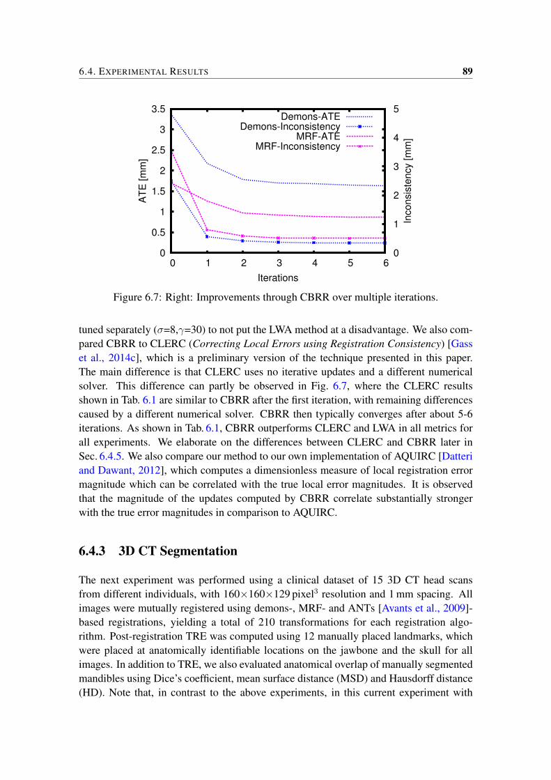
6.4. EXPERIMENTAL RESULTS 89
0
0.5
1
1.5
2
2.5
3
3.5
0 1 2 3 4 5 6 0
1
2
3
4
5
AT
E [
mm
]
Inco
nsis
ten
cy [
mm
]
Iterations
Demons-ATEDemons-Inconsistency
MRF-ATEMRF-Inconsistency
Figure 6.7: Right: Improvements through CBRR over multiple iterations.
tuned separately (σ=8,γ=30) to not put the LWA method at a disadvantage. We also com-pared CBRR to CLERC (Correcting Local Errors using Registration Consistency) [Gasset al., 2014c], which is a preliminary version of the technique presented in this paper.The main difference is that CLERC uses no iterative updates and a different numericalsolver. This difference can partly be observed in Fig. 6.7, where the CLERC resultsshown in Tab. 6.1 are similar to CBRR after the first iteration, with remaining differencescaused by a different numerical solver. CBRR then typically converges after about 5-6iterations. As shown in Tab. 6.1, CBRR outperforms CLERC and LWA in all metrics forall experiments. We elaborate on the differences between CLERC and CBRR later inSec. 6.4.5. We also compare our method to our own implementation of AQUIRC [Datteriand Dawant, 2012], which computes a dimensionless measure of local registration errormagnitude which can be correlated with the true local error magnitudes. It is observedthat the magnitude of the updates computed by CBRR correlate substantially strongerwith the true error magnitudes in comparison to AQUIRC.
6.4.3 3D CT Segmentation
The next experiment was performed using a clinical dataset of 15 3D CT head scansfrom different individuals, with 160×160×129 pixel3 resolution and 1 mm spacing. Allimages were mutually registered using demons-, MRF- and ANTs [Avants et al., 2009]-based registrations, yielding a total of 210 transformations for each registration algo-rithm. Post-registration TRE was computed using 12 manually placed landmarks, whichwere placed at anatomically identifiable locations on the jawbone and the skull for allimages. In addition to TRE, we also evaluated anatomical overlap of manually segmentedmandibles using Dice’s coefficient, mean surface distance (MSD) and Hausdorff distance(HD). Note that, in contrast to the above experiments, in this current experiment with
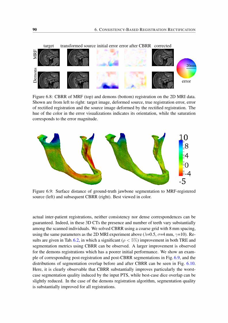
90 6. CONSISTENCY-BASED REGISTRATION RECTIFICATION
target transformed source initial error error after CBRR corrected
MR
F
20mm
errorDem
ons
Figure 6.8: CBRR of MRF (top) and demons (bottom) registration on the 2D MRI data.Shown are from left to right: target image, deformed source, true registration error, errorof rectified registration and the source image deformed by the rectified registration. Thehue of the color in the error visualizations indicates its orientation, while the saturationcorresponds to the error magnitude.
Figure 6.9: Surface distance of ground-truth jawbone segmentation to MRF-registeredsource (left) and subsequent CBRR (right). Best viewed in color.
actual inter-patient registrations, neither consistency nor dense correspondences can beguaranteed. Indeed, in these 3D CTs the presence and number of teeth vary substantiallyamong the scanned individuals. We solved CBRR using a coarse grid with 8 mm spacing,using the same parameters as the 2D MRI experiment above (λ=0.5, σ=4 mm, γ=10). Re-sults are given in Tab. 6.2, in which a significant (ρ < 5%) improvement in both TRE andsegmentation metrics using CBRR can be observed. A larger improvement is observedfor the demons registrations which has a poorer initial performance. We show an exam-ple of corresponding post-registration and post-CBRR segmentations in Fig. 6.9, and thedistributions of segmentation overlap before and after CBRR can be seen in Fig. 6.10.Here, it is clearly observable that CBRR substantially improves particularly the worst-case segmentation quality induced by the input PTS, while best-case dice overlap can beslightly reduced. In the case of the demons registration algorithm, segmentation qualityis substantially improved for all registrations.
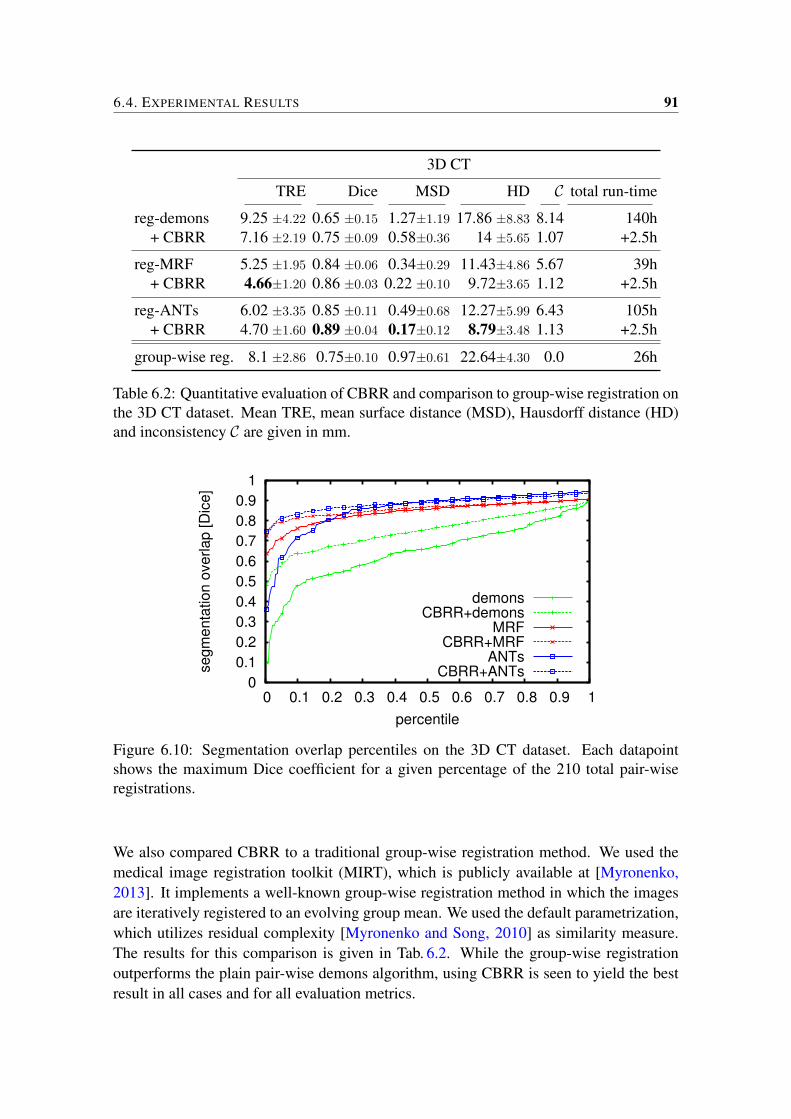
6.4. EXPERIMENTAL RESULTS 91
3D CT
TRE Dice MSD HD C total run-time
reg-demons 9.25 ±4.22 0.65 ±0.15 1.27±1.19 17.86 ±8.83 8.14 140h+ CBRR 7.16 ±2.19 0.75 ±0.09 0.58±0.36 14 ±5.65 1.07 +2.5h
reg-MRF 5.25 ±1.95 0.84 ±0.06 0.34±0.29 11.43±4.86 5.67 39h+ CBRR 4.66±1.20 0.86 ±0.03 0.22 ±0.10 9.72±3.65 1.12 +2.5h
reg-ANTs 6.02 ±3.35 0.85 ±0.11 0.49±0.68 12.27±5.99 6.43 105h+ CBRR 4.70 ±1.60 0.89 ±0.04 0.17±0.12 8.79±3.48 1.13 +2.5h
group-wise reg. 8.1 ±2.86 0.75±0.10 0.97±0.61 22.64±4.30 0.0 26h
Table 6.2: Quantitative evaluation of CBRR and comparison to group-wise registration onthe 3D CT dataset. Mean TRE, mean surface distance (MSD), Hausdorff distance (HD)and inconsistency C are given in mm.
0
0.1
0.2
0.3
0.4
0.5
0.6
0.7
0.8
0.9
1
0 0.1 0.2 0.3 0.4 0.5 0.6 0.7 0.8 0.9 1
segm
enta
tion o
verlap [D
ice]
percentile
demonsCBRR+demons
MRFCBRR+MRF
ANTsCBRR+ANTs
Figure 6.10: Segmentation overlap percentiles on the 3D CT dataset. Each datapointshows the maximum Dice coefficient for a given percentage of the 210 total pair-wiseregistrations.
We also compared CBRR to a traditional group-wise registration method. We used themedical image registration toolkit (MIRT), which is publicly available at [Myronenko,2013]. It implements a well-known group-wise registration method in which the imagesare iteratively registered to an evolving group mean. We used the default parametrization,which utilizes residual complexity [Myronenko and Song, 2010] as similarity measure.The results for this comparison is given in Tab. 6.2. While the group-wise registrationoutperforms the plain pair-wise demons algorithm, using CBRR is seen to yield the bestresult in all cases and for all evaluation metrics.
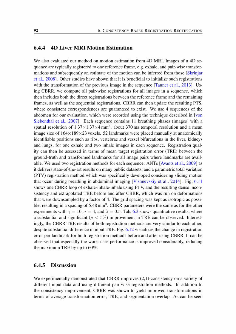
92 6. CONSISTENCY-BASED REGISTRATION RECTIFICATION
6.4.4 4D Liver MRI Motion Estimation
We also evaluated our method on motion estimation from 4D MRI. Images of a 4D se-quence are typically registered to one reference frame, e.g. exhale, and pair-wise transfor-mations and subsequently an estimate of the motion can be inferred from those [Skrinjaret al., 2008]. Other studies have shown that it is beneficial to initialize such registrationswith the transformation of the previous image in the sequence [Tanner et al., 2013]. Us-ing CBRR, we compute all pair-wise registrations for all images in a sequence, whichthen includes both the direct registrations between the reference frame and the remainingframes, as well as the sequential registrations. CBRR can then update the resulting PTS,where consistent correspondences are guaranteed to exist. We use 4 sequences of theabdomen for our evaluation, which were recorded using the technique described in [vonSiebenthal et al., 2007]. Each sequence contains 11 breathing phases (images) with aspatial resolution of 1.37×1.37×4 mm3, about 370 ms temporal resolution and a meanimage size of 164×189×23 voxels. 52 landmarks were placed manually at anatomicallyidentifiable positions such as ribs, vertebrae and vessel bifurcations in the liver, kidneysand lungs, for one exhale and two inhale images in each sequence. Registration qual-ity can then be assessed in terms of mean target registration error (TRE) between theground-truth and transformed landmarks for all image pairs where landmarks are avail-able. We used two registration methods for each sequence: ANTs [Avants et al., 2009] asit delivers state-of-the-art results on many public datasets, and a parametric total variation(PTV) registration method which was specifically developed considering sliding motionthat occur during breathing in abdominal imaging [Vishnevskiy et al., 2014]. Fig. 6.11shows one CBRR loop of exhale-inhale-inhale using PTV, and the resulting dense incon-sistency and extrapolated TRE before and after CBRR, which was run on deformationsthat were downsampled by a factor of 4. The grid spacing was kept as isotropic as possi-ble, resulting in a spacing of 5.48 mm3. CBRR parameters were the same as for the otherexperiments with γ = 10, σ = 4, and λ = 0.5. Tab. 6.3 shows quantitative results, wherea substantial and significant (ρ < 5%) improvement in TRE can be observed. Interest-ingly, the CBRR TRE results of both registration methods are very similar to each other,despite substantial difference in input TRE. Fig. 6.12 visualizes the change in registrationerror per landmark for both registration methods before and after using CBRR. It can beobserved that especially the worst-case performance is improved considerably, reducingthe maximum TRE by up to 60%.
6.4.5 Discussion
We experimentally demonstrated that CBRR improves (2,1)-consistency on a variety ofdifferent input data and using different pair-wise registration methods. In addition tothe consistency improvement, CBRR was shown to yield improved transformations interms of average transformation error, TRE, and segmentation overlap. As can be seen
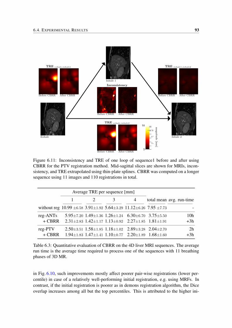
6.4. EXPERIMENTAL RESULTS 93
Exhale Inhale 2
Inhale 1
Inconsistency
Before CBRR After CBRR
magnitu
de[m
m]
TRE exhale,inhale2
Before CBRR After CBRR
TRE exhale,inhale1
Before CBRR After CBRR
TRE inhale1,inhale2
Before CBRR After CBRR
Figure 6.11: Inconsistency and TRE of one loop of sequence1 before and after usingCBRR for the PTV registration method. Mid-sagittal slices are shown for MRIs, incon-sistency, and TRE extrapolated using thin-plate splines. CBRR was computed on a longersequence using 11 images and 110 registrations in total.
Average TRE per sequence [mm]
1 2 3 4 total mean avg. run-time
without reg 10.99 ±6.58 3.91±1.92 5.64±3.29 11.12±6.26 7.95 ±7.73 -
reg-ANTs 5.95±7.20 1.49±1.36 1.26±1.24 6.30±6.70 3.75±5.50 10h+ CBRR 2.31±2.83 1.42±1.17 1.13±0.92 2.27±1.85 1.81±1.91 +3h
reg-PTV 2.50±3.51 1.58±1.85 1.18±1.02 2.89±3.28 2.04±2.70 2h+ CBRR 1.94±1.83 1.47±1.41 1.10±0.77 2.20±1.89 1.68±1.60 +3h
Table 6.3: Quantitative evaluation of CBRR on the 4D liver MRI sequences. The averagerun time is the average time required to process one of the sequences with 11 breathingphases of 3D MR.
in Fig. 6.10, such improvements mostly affect poorer pair-wise registrations (lower per-centile) in case of a relatively well-performing initial registration, e.g. using MRFs. Incontrast, if the initial registration is poorer as in demons registration algorithm, the Diceoverlap increases among all but the top percentiles. This is attributed to the higher ini-
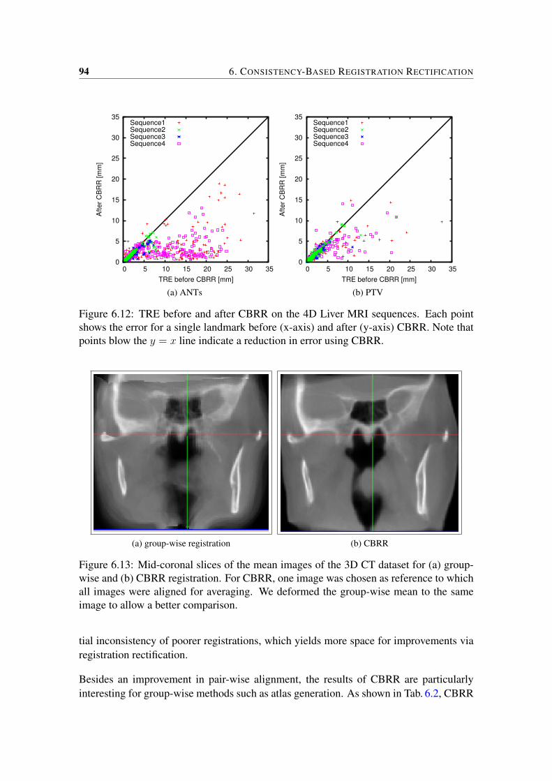
94 6. CONSISTENCY-BASED REGISTRATION RECTIFICATION
0
5
10
15
20
25
30
35
0 5 10 15 20 25 30 35
Aft
er
CB
RR
[m
m]
TRE before CBRR [mm]
Sequence1Sequence2Sequence3Sequence4
(a) ANTs
0
5
10
15
20
25
30
35
0 5 10 15 20 25 30 35
Aft
er
CB
RR
[m
m]
TRE before CBRR [mm]
Sequence1Sequence2Sequence3Sequence4
(b) PTV
Figure 6.12: TRE before and after CBRR on the 4D Liver MRI sequences. Each pointshows the error for a single landmark before (x-axis) and after (y-axis) CBRR. Note thatpoints blow the y = x line indicate a reduction in error using CBRR.
(a) group-wise registration (b) CBRR
Figure 6.13: Mid-coronal slices of the mean images of the 3D CT dataset for (a) group-wise and (b) CBRR registration. For CBRR, one image was chosen as reference to whichall images were aligned for averaging. We deformed the group-wise mean to the sameimage to allow a better comparison.
tial inconsistency of poorer registrations, which yields more space for improvements viaregistration rectification.
Besides an improvement in pair-wise alignment, the results of CBRR are particularlyinteresting for group-wise methods such as atlas generation. As shown in Tab. 6.2, CBRR
6.4. EXPERIMENTAL RESULTS 95
can out-perform group-wise registration quantitatively. A typical qualitative result ofgroup-wise registration is the resulting mean image, which represents the center of thedistribution. Here, a sharp mean image is an indicator for the successful alignment of allimages to such mean. We present mean images using registrations from CBRR and group-wise registrations in Fig. 6.13. Since CBRR does not return the center of the distributiondirectly, the images are in the reference space of one randomly chosen image for bettercomparison. It can be seen that the CBRR mean is much sharper than the group-wisemean, indicating that group-wise registration could not align the images satisfactorily inthis task.
Note that CBRR yields satisfactory results in all tests with an uniform parametrization.Note that further experiment-specific improvement is possible, in particular by adjustingλ to incorporate prior knowledge on the expected error. Different choices of the localsimilarity metric can also be beneficial, especially for multi-modal data.
CBRR can also be interpreted as a detection method for inconsistency-based registrationerrors. Based on the difference between the estimated and the original registrations, onecan estimate local error magnitudes. These estimations can be evaluated through ground-truth local-error magnitudes, for experiments for which those are known. This allows for acomparison with AQUIRC [Datteri and Dawant, 2012], which computes a dimension-lessmeasure of local error magnitude based on (3,0)-consistency. We used our own implemen-tation of their technique, the results of which were presented in Tab. 6.1. Note that CBRRcould also be adapted to utilize (3,0)-consistency, but would require an additional approx-imation (c.f. Sec. 6.3.3) for the additional transformation composition, which would makethe implementation more complicated and the solution less robust. The error magnitudesestimated by CBRR correlate much stronger with the true error magnitudes in compar-ison to AQUIRC, in addition to surpassing our earlier algorithm CLERC [Gass et al.,2014c]. Additionally, both CLERC and CBRR estimate actual error vectors in contrast tothe dimension-less measure being reported by AQUIRC. The difference in performancebetween CBRR and CLERC can mainly be explained through the additional iterative re-finement in CBRR, which improves the approximation in (6.12). An additional benefit ofCBRR is that it requires to only estimate registration variables, in contrast to registrationand error variables in CLERC. This makes it computationally more efficient and easier toparametrize since one less parameter is required.
Still, the bottleneck of the proposed CBRR algorithm is its large memory requirementsince all the displacement variables are estimated simultaneously. This contrasts theAQUIRC approach [Datteri and Dawant, 2012], which can solve for the error at everyspatial location independently. In our experiments, the memory utilization reached up to15 GB for the 3D CT segmentation experiment. The main factor for this is the numberof non-zero entries in A, which is proportional to N3M , where M denotes the numberof coarse grid points. Note that we keep only the downsampled pair-wise registrationsin memory, while re-loading the full resolution registrations only on demand. We imple-mented our CBRR prototype in C++/ITK. Constructed systems of equations are solved
96 6. CONSISTENCY-BASED REGISTRATION RECTIFICATION
using the minFunc solver called via the Matlab engine interface for C++. The equationsystem itself is not particularly large in memory, requiring about 6GB including all auxil-iary variables for the 15 3D CT image problem. However, a significant memory overheadis needed in Matlab for passing and solving the problem. Therefore, using a dedicatedC++ solver might be one approach to reducing memory demands. Additionally, our ex-periments showed that satisfactory results can be already achieved with a limited numberof images (c.f. Fig. 6.6). For instance, reducing the number of images from 15 to 7 inthe 3D case would reduce the memory requirements by a factor of 8. One advantage ofCBRR is the speed with which all pair-wise registrations are updated. One full iteration,which updates 210 3D registrations, takes about 30 minutes, including the computationof pair-wise local similarities. This is about 80 times as fast as computing all pair-wiseregistrations using MRFs. Since the proposed approach is likely to be used in an offlinefashion, it would be reasonable to trade off run-time for decreased memory usage, therebyalso allowing for more images and/or higher resolution transformations.
A strong point of CBRR is that it is independent of the used registration algorithm, andimposes no restrictions on the spatial smoothness of the transformations. This enablesits application also in challenging scenarios as in registration with sliding motion, as canbe seen from the results on the 4D MRI experiment, where substantial improvements areseen both for a smooth (ANTs) and for a sliding-motion enabled registration method.
6.5 Conclusions
We presented a novel population-based method for refining pair-wise registrations byreducing their inconsistency. By formulating the task as a linear least-squares problem,we obtain an efficient algorithm that is able to resolve such inconsistencies in groups ofup to 15 3D images simultaneously, which is, to the best of our knowledge, not possiblewith any other technique. In contrast to group-wise registration, our method is arguablybetter suited for inter-patient registration, as correspondences need not be perfect acrossall images. Instead, a trade-off is achieved, balancing group-wise consistency and pair-wise visual similarity. Experimentally, our approach was shown to be able to not onlyincrease consistency, but also improve segmentation overlap in atlas-based segmentation,and target registration error in both inter- and intra-patient registration, where the latter isan important problem e.g. for breathing motion estimation.
7Summary and Perspectives
In this thesis, several methods for medical image segmentation using weak priors havebeen presented. Each chapter was published separately in peer-reviewed journals andconference proceedings. Since each article, and therefore chapter, already contains aspecific discussion of the presented algorithm and perspectives, this summary focuses onmore generic observations and implications.
In Chap. 2, an iterative algorithm for joint segmentation and registration has been inves-tigated that utilizes the given segmentation of an atlas and penalizes deviations betweendeformed atlas segmentation and an intensity-based segmentation of the target image us-ing a distance function. This allows the optimization to avoid poor local optima in earlystages of the iterative registration. Still, this definition of the joint segmentation and reg-istration problem is inherently ill-posed as such since it relies on the overlap between thedeformed atlas segmentation and any voxel which matches the intensity model of the tar-get anatomy. In medical imaging, such intensity models are often not organ-, but rathertissue-specific, e.g. the well-known threshold in Hounsfield units for the bone. To create amore robust optimization problem, it has been proposed in this chapter to use an auxiliarysegmentation label in both atlas and target, which accounts for any structure that fits theintensity model but does not cover the target anatomy.
Chap. 3 extends on the previous chapter by developing a simultaneous non-rigid regis-tration and segmentation (SRS) method, in contrast to many studies in the literature thatutilize alternating optimization schemes. The goal function is obtained through a rigor-ous analysis of the underlying MAP problem, and a novel two-layer Markov random fieldis proposed which allows for estimating registration and segmentation variables at differ-ent levels of detail. As one of the first studies in the literature, the presented approachallows for the direct comparison of alternating and simultaneous solvers for this problem,and it is demonstrated that SRS achieves superior segmentation fidelity in terms of bothoverlap- and distance based criteria. Such improvements over standard registration-basedsegmentation and the alternating approach have been mainly observed in the lower per-centiles with regard to pair-wise post registration segmentation overlap in a leave-one-outstudy. This demonstrates the increased robustness with regard to atlas-target mismatch or
98 7. SUMMARY AND PERSPECTIVES
poor local optima. While achieving the best segmentation quality on the 3D CT datasetof all algorithms presented in this thesis, the presented method has two drawbacks: (i)the registration algorithm uses to a discrete optimization scheme, and (which might notbe preferable for a specific application, or available due to patents on the optimizationtechniques) (ii) there are eight free parameters which need to be set specifically for eachtask.
The algorithms presented in the remaining chapters of this thesis address these challengesby utilizing semi-supervised techniques which can leverage information from sets of un-segmented images. Crucially, they all act as post-processing given a set of non-rigidregistrations as input. This addresses challenge (i) of the previous section since it allowsfor using the result of any available registration algorithm. This can be important forclinical applications where personnel might be familiar with or constrained to a specificimplementation in their work-flow. Furthermore, it can be observed that the algorithms inthe following chapters use fewer parameters (two in Chap. 4 and three in chapters 5 and6) in addition to those used by the registration. Those parameters generalize quite welland can be applied with little adjustments when dealing with different segmentation tasksand image modalities. This is a major benefit which makes it much easier, in comparisonto SRS, to use those semi-supervised methods out-of-the-box.
To differentiate further, the algorithms presented in chapters 4 and 5, respectively, com-bine automatically generated segmentation and registration hypotheses. In both cases, itis assumed that the intermediate registration steps between atlas and target may containinformation which complements the direct registration of atlas and target. This is consis-tent with the literature, where it was frequently observed that a certain fit between atlasand target images is necessary to obtain satisfactory segmentation performance when us-ing conventional atlas-based segmentation. This challenge can at least partly be overcomeby the proposed methods, as also observed from the segmentation results which exhibitincreased robustness with regard to atlas selection (c.f. Fig. 4.3a).
The algorithm presented in Chap. 6 aims at a similar goal compared to the previous twochapters, but replaces the heuristic fusion of segmentation/registration hypotheses witha more principled goal function: By optimizing the consistency of the set of pair-wiseregistrations in a least-squares optimization framework, information from all pair-wiseregistrations are combined in order to update all pair-wise registrations simultaneously.Interestingly, this approach can not surpass the registration and segmentation fidelity ofthe algorithms presented in chapters 4 and 5. This can be attributed to the cubic complex-ity of CBRR with regard to the number of images, in contrast to the quadratic complexityof the other two methods. This necessitates a coarser control grid resolution (8 px inCBRR vs. 4 px in MRegFuse), which prohibits an explicit computation of high-frequencydeformation detail. However, the registrations computed by CBRR have the benefit ofbeing optimized for registration consistency, which can be useful in certain scenarios asdiscussed in the following.

99
The algorithms presented in this thesis have been demonstrated to improve the fidelity ofregistration-based segmentation methods using weak priors. It is important to considerthe different use-cases for such automatically generated segmentations. While they canbe used directly, for example to guide dose estimation in radiotherapy, a set of segmentedimages can also be used to generate strong prior knowledge, for example in the formof a statistical shape model. The use of such automatically generated segmentations incontrast to manual, gold-standard segmentations for the generation of strong prior knowl-edge has not yet been studied comprehensively and shall be a topic for further research.For the purpose of generating such models with strong prior knowledge, it is especiallyinteresting to consider other additional information besides the segmentation results thatis generated by the proposed algorithms. For example, the consistent registrations ofCBRR can contribute to solving the challenging correspondence problem in statisticalshape model generation from binary segmentations.
In the future, it will be interesting to further investigate both weak prior combinations andsemi-supervised segmentation methods. As demonstrated in this thesis, it can be benefi-cial to formulate target criteria which are as similar to the intended goal as possible. Also,the exploration of correspondences between unsegmented images appears promising forthe advancement of segmentation algorithms. While often being computationally chal-lenging, pair-wise registrations between such unsegmented images may carry valuableinformation which have not yet been widely used. In this thesis, this approach has beendemonstrated to benefit even small sets of images with strong variability, where commongroup-wise methods do not perform satisfactorily.


Bibliography
[Ali et al., 2007] Ali, A., Farag, A., and El-Baz, A. (2007). Graph Cuts Framework forKidney Segmentation with Prior Shape Constraints. In Ayache, N., Ourselin, S., andMaeder, A., editors, Proc. Medical Image Computing and Computer-Assisted Inter-vention, volume 4791 of Lecture Notes in Computer Science, pages 384–392. SpringerBerlin Heidelberg. 1.2.1.3
[Avants et al., 2008a] Avants, B., Epstein, C., Grossman, M., and Gee, J. (2008a). Sym-metric Diffeomorphic Image Registration with Cross-Correlation: Evaluating Auto-mated Labeling of Elderly and Neurodegenerative Brain. Medical Image Analysis,12(1):26–41. 5.1
[Avants et al., 2009] Avants, B., Tustison, N., and Song, G. (2009). Advanced Normal-ization Tools (ANTS). Insight Journal, pages 1–35. 6.4.3, 6.4.4
[Avants et al., 2008b] Avants, B. B., Epstein, C. L., Grossman, M., and Gee, J. C.(2008b). Symmetric diffeomorphic image registration with cross-correlation: evalu-ating automated labeling of elderly and neurodegenerative brain. Medical Image Anal-ysis, 12(1):26–41. 6.1
[Balci et al., 2007] Balci, S. K., Golland, P., Shenton, M., and Wells, W. (2007). Free-form B-spline deformation model for groupwise registration. In Proc. Medical ImageComputing and Computer-Assisted Intervention, volume 10, pages 23–30. NIH PublicAccess. 1.2.2
[Bhatia and Hajnal, 2004] Bhatia, K. K. and Hajnal, J. (2004). Consistent groupwisenon-rigid registration for atlas construction. In Proc IEEE International Symposiumon Biomedical Imaging, pages 908–911. 6.1
[Blanc et al., 2009] Blanc, R., Reyes, M., Seiler, C., and Székely, G. (2009). Conditionalvariability of statistical shape models based on surrogate variables. In Proc. MedicalImage Computing and Computer-Assisted Intervention, pages 84–91. 1.3
[Blezek and Miller, 2007] Blezek, D. and Miller, J. (2007). Atlas stratification. MedicalImage Analysis, 11(5):443–457. 1.3
[Bondiau et al., 2005] Bondiau, P.-Y., Malandain, G., Chanalet, S., Marcy, P.-Y.,Habrand, J.-L., Fauchon, F., Paquis, P., Courdi, A., Commowick, O., Rutten, I., andAyache, N. (2005). Atlas-based automatic segmentation of MR images: validation
102 BIBLIOGRAPHY
study on the brainstem in radiotherapy context. International journal of radiation on-cology, biology, physics, 61(1):289–98. 1
[Bornik et al., 2006] Bornik, A., Beichel, R., and Schmalstieg, D. (2006). Interactiveediting of segmented volumetric datasets in a hybrid 2D/3D virtual environment. Pro-ceedings of the ACM symposium on Virtual reality software and technology - VRST’06, page 197. 1.1
[Boykov and Funke-Lea, 2006] Boykov, Y. and Funke-Lea, G. (2006). Graph Cutsand Efficient N-D Image Segmentation. International Journal of Computer Vision,70(2):109–131. 2.1, 3.1, 3.2, 4.1
[Boykov and Jolly, 2000] Boykov, Y. and Jolly, M.-p. (2000). Interactive Organ Segmen-tation Using Graph Cuts. Organ, The, pages 276–286. 1.2.1.1, 3.2, 3.4.3.1
[Boykov et al., 2001] Boykov, Y., Veksler, O., and Zabih, R. (2001). Fast ApproximateEnergy Minimization via Graph Cuts. IEEE Transactions on Pattern Analysis andMachine Intelligence, 23(11):1222–1239. 2.2, 2.3.1, 3.4.3.1
[Breiman, 2001] Breiman, L. (2001). Random forests. Machine learning, 45(1):5–32.1.2.1.1, 2.3, 3.4.3.1
[Cachier and Ayache, 2001] Cachier, P. and Ayache, N. (2001). Regularization in ImageNon-Rigid Registration: I. Trade-off between Smoothness and Intensity Similarity.Technical report, INRIA. 5.1
[Cachier et al., 2003] Cachier, P., Bardinet, E., Dormont, D., Pennec, X., and Ayache, N.(2003). Iconic feature based nonrigid registration: the PASHA algorithm. ComputerVision and Image Understanding, 89(2-3):272–298. 3.6, 5.2, 6.3.2
[Cardoso et al., 2012] Cardoso, M. J., Modat, M., Ourselin, S., Keihaninejad, S., andCash, D. (2012). Multi-STEPS: Multi-label similarity and truth estimation for propa-gated segmentations. In Mathematical Methods in Biomedical Image Analysis, pages153–158. 5.2, 6.3.2
[Chapelle et al., 2006] Chapelle, O., Schölkopf, B., and Zien, A., editors (2006). Semi-supervised learning, volume 2. MIT press Cambridge, MA. 1.2.2, 4.1
[Christensen and Johnson, 2001] Christensen, G. E. and Johnson, H. J. (2001). Consis-tent image registration. IEEE Transactions on Medical Imaging, 20(7):568–582. 6.1,6.2
[Christensen and Johnson, 2003] Christensen, G. E. and Johnson, H. J. (2003). Invert-ibility and transitivity analysis for nonrigid image registration. Journal of ElectronicImaging, 12(1):106. 6.2
[Christensen et al., 1995] Christensen, G. E., Rabbitt, R. D., Miller, M. I., Joshi, S. C.,Grenander, U., and Coogan, T. A. (1995). Topological Properties of Smooth AnatomicMaps. In Proc. Information Processing in Medical Imaging, pages 101–112. Springer.5.3
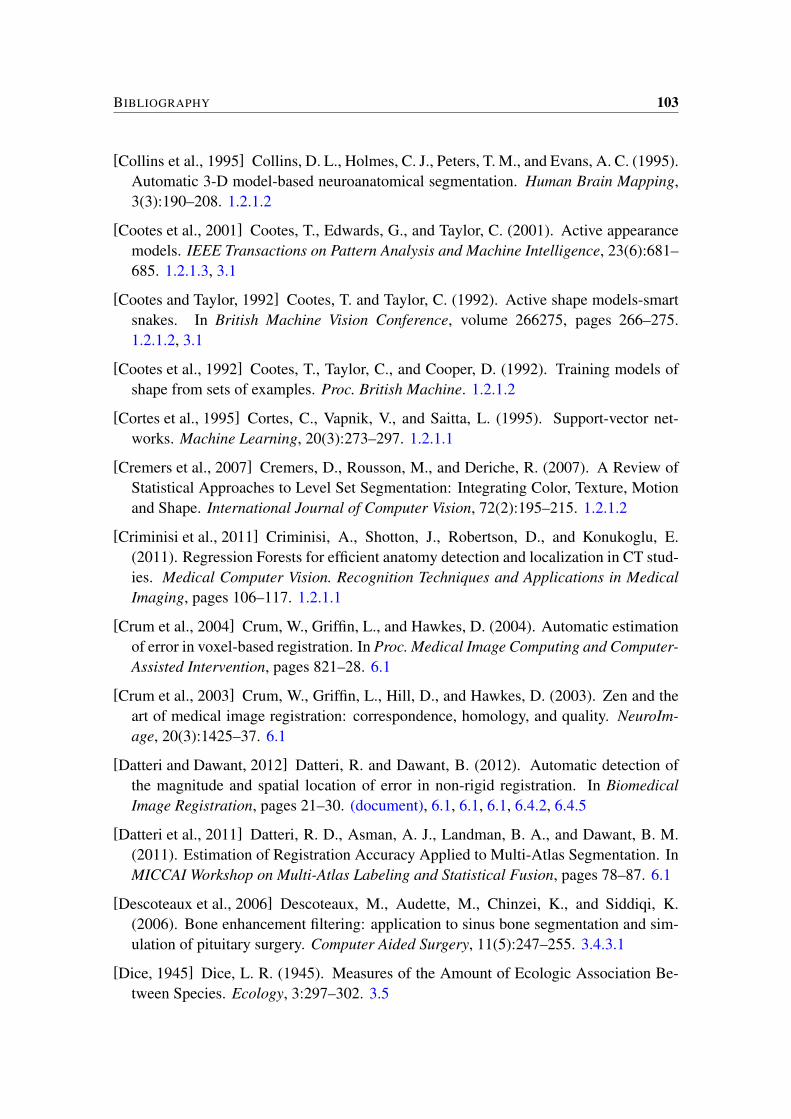
BIBLIOGRAPHY 103
[Collins et al., 1995] Collins, D. L., Holmes, C. J., Peters, T. M., and Evans, A. C. (1995).Automatic 3-D model-based neuroanatomical segmentation. Human Brain Mapping,3(3):190–208. 1.2.1.2
[Cootes et al., 2001] Cootes, T., Edwards, G., and Taylor, C. (2001). Active appearancemodels. IEEE Transactions on Pattern Analysis and Machine Intelligence, 23(6):681–685. 1.2.1.3, 3.1
[Cootes and Taylor, 1992] Cootes, T. and Taylor, C. (1992). Active shape models-smartsnakes. In British Machine Vision Conference, volume 266275, pages 266–275.1.2.1.2, 3.1
[Cootes et al., 1992] Cootes, T., Taylor, C., and Cooper, D. (1992). Training models ofshape from sets of examples. Proc. British Machine. 1.2.1.2
[Cortes et al., 1995] Cortes, C., Vapnik, V., and Saitta, L. (1995). Support-vector net-works. Machine Learning, 20(3):273–297. 1.2.1.1
[Cremers et al., 2007] Cremers, D., Rousson, M., and Deriche, R. (2007). A Review ofStatistical Approaches to Level Set Segmentation: Integrating Color, Texture, Motionand Shape. International Journal of Computer Vision, 72(2):195–215. 1.2.1.2
[Criminisi et al., 2011] Criminisi, A., Shotton, J., Robertson, D., and Konukoglu, E.(2011). Regression Forests for efficient anatomy detection and localization in CT stud-ies. Medical Computer Vision. Recognition Techniques and Applications in MedicalImaging, pages 106–117. 1.2.1.1
[Crum et al., 2004] Crum, W., Griffin, L., and Hawkes, D. (2004). Automatic estimationof error in voxel-based registration. In Proc. Medical Image Computing and Computer-Assisted Intervention, pages 821–28. 6.1
[Crum et al., 2003] Crum, W., Griffin, L., Hill, D., and Hawkes, D. (2003). Zen and theart of medical image registration: correspondence, homology, and quality. NeuroIm-age, 20(3):1425–37. 6.1
[Datteri and Dawant, 2012] Datteri, R. and Dawant, B. (2012). Automatic detection ofthe magnitude and spatial location of error in non-rigid registration. In BiomedicalImage Registration, pages 21–30. (document), 6.1, 6.1, 6.1, 6.4.2, 6.4.5
[Datteri et al., 2011] Datteri, R. D., Asman, A. J., Landman, B. A., and Dawant, B. M.(2011). Estimation of Registration Accuracy Applied to Multi-Atlas Segmentation. InMICCAI Workshop on Multi-Atlas Labeling and Statistical Fusion, pages 78–87. 6.1
[Descoteaux et al., 2006] Descoteaux, M., Audette, M., Chinzei, K., and Siddiqi, K.(2006). Bone enhancement filtering: application to sinus bone segmentation and sim-ulation of pituitary surgery. Computer Aided Surgery, 11(5):247–255. 3.4.3.1
[Dice, 1945] Dice, L. R. (1945). Measures of the Amount of Ecologic Association Be-tween Species. Ecology, 3:297–302. 3.5
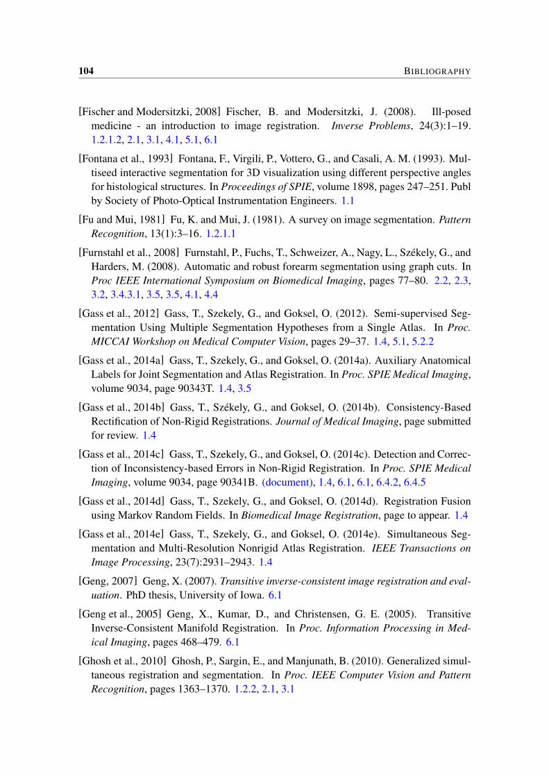
104 BIBLIOGRAPHY
[Fischer and Modersitzki, 2008] Fischer, B. and Modersitzki, J. (2008). Ill-posedmedicine - an introduction to image registration. Inverse Problems, 24(3):1–19.1.2.1.2, 2.1, 3.1, 4.1, 5.1, 6.1
[Fontana et al., 1993] Fontana, F., Virgili, P., Vottero, G., and Casali, A. M. (1993). Mul-tiseed interactive segmentation for 3D visualization using different perspective anglesfor histological structures. In Proceedings of SPIE, volume 1898, pages 247–251. Publby Society of Photo-Optical Instrumentation Engineers. 1.1
[Fu and Mui, 1981] Fu, K. and Mui, J. (1981). A survey on image segmentation. PatternRecognition, 13(1):3–16. 1.2.1.1
[Furnstahl et al., 2008] Furnstahl, P., Fuchs, T., Schweizer, A., Nagy, L., Székely, G., andHarders, M. (2008). Automatic and robust forearm segmentation using graph cuts. InProc IEEE International Symposium on Biomedical Imaging, pages 77–80. 2.2, 2.3,3.2, 3.4.3.1, 3.5, 3.5, 4.1, 4.4
[Gass et al., 2012] Gass, T., Szekely, G., and Goksel, O. (2012). Semi-supervised Seg-mentation Using Multiple Segmentation Hypotheses from a Single Atlas. In Proc.MICCAI Workshop on Medical Computer Vision, pages 29–37. 1.4, 5.1, 5.2.2
[Gass et al., 2014a] Gass, T., Szekely, G., and Goksel, O. (2014a). Auxiliary AnatomicalLabels for Joint Segmentation and Atlas Registration. In Proc. SPIE Medical Imaging,volume 9034, page 90343T. 1.4, 3.5
[Gass et al., 2014b] Gass, T., Székely, G., and Goksel, O. (2014b). Consistency-BasedRectification of Non-Rigid Registrations. Journal of Medical Imaging, page submittedfor review. 1.4
[Gass et al., 2014c] Gass, T., Szekely, G., and Goksel, O. (2014c). Detection and Correc-tion of Inconsistency-based Errors in Non-Rigid Registration. In Proc. SPIE MedicalImaging, volume 9034, page 90341B. (document), 1.4, 6.1, 6.1, 6.4.2, 6.4.5
[Gass et al., 2014d] Gass, T., Szekely, G., and Goksel, O. (2014d). Registration Fusionusing Markov Random Fields. In Biomedical Image Registration, page to appear. 1.4
[Gass et al., 2014e] Gass, T., Szekely, G., and Goksel, O. (2014e). Simultaneous Seg-mentation and Multi-Resolution Nonrigid Atlas Registration. IEEE Transactions onImage Processing, 23(7):2931–2943. 1.4
[Geng, 2007] Geng, X. (2007). Transitive inverse-consistent image registration and eval-uation. PhD thesis, University of Iowa. 6.1
[Geng et al., 2005] Geng, X., Kumar, D., and Christensen, G. E. (2005). TransitiveInverse-Consistent Manifold Registration. In Proc. Information Processing in Med-ical Imaging, pages 468–479. 6.1
[Ghosh et al., 2010] Ghosh, P., Sargin, E., and Manjunath, B. (2010). Generalized simul-taneous registration and segmentation. In Proc. IEEE Computer Vision and PatternRecognition, pages 1363–1370. 1.2.2, 2.1, 3.1
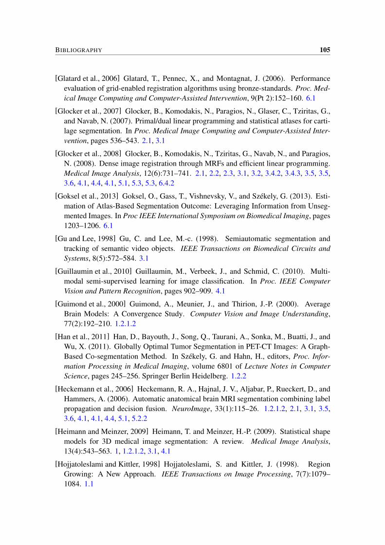
BIBLIOGRAPHY 105
[Glatard et al., 2006] Glatard, T., Pennec, X., and Montagnat, J. (2006). Performanceevaluation of grid-enabled registration algorithms using bronze-standards. Proc. Med-ical Image Computing and Computer-Assisted Intervention, 9(Pt 2):152–160. 6.1
[Glocker et al., 2007] Glocker, B., Komodakis, N., Paragios, N., Glaser, C., Tziritas, G.,and Navab, N. (2007). Primal/dual linear programming and statistical atlases for carti-lage segmentation. In Proc. Medical Image Computing and Computer-Assisted Inter-vention, pages 536–543. 2.1, 3.1
[Glocker et al., 2008] Glocker, B., Komodakis, N., Tziritas, G., Navab, N., and Paragios,N. (2008). Dense image registration through MRFs and efficient linear programming.Medical Image Analysis, 12(6):731–741. 2.1, 2.2, 2.3, 3.1, 3.2, 3.4.2, 3.4.3, 3.5, 3.5,3.6, 4.1, 4.4, 4.1, 5.1, 5.3, 5.3, 6.4.2
[Goksel et al., 2013] Goksel, O., Gass, T., Vishnevsky, V., and Székely, G. (2013). Esti-mation of Atlas-Based Segmentation Outcome: Leveraging Information from Unseg-mented Images. In Proc IEEE International Symposium on Biomedical Imaging, pages1203–1206. 6.1
[Gu and Lee, 1998] Gu, C. and Lee, M.-c. (1998). Semiautomatic segmentation andtracking of semantic video objects. IEEE Transactions on Biomedical Circuits andSystems, 8(5):572–584. 3.1
[Guillaumin et al., 2010] Guillaumin, M., Verbeek, J., and Schmid, C. (2010). Multi-modal semi-supervised learning for image classification. In Proc. IEEE ComputerVision and Pattern Recognition, pages 902–909. 4.1
[Guimond et al., 2000] Guimond, A., Meunier, J., and Thirion, J.-P. (2000). AverageBrain Models: A Convergence Study. Computer Vision and Image Understanding,77(2):192–210. 1.2.1.2
[Han et al., 2011] Han, D., Bayouth, J., Song, Q., Taurani, A., Sonka, M., Buatti, J., andWu, X. (2011). Globally Optimal Tumor Segmentation in PET-CT Images: A Graph-Based Co-segmentation Method. In Székely, G. and Hahn, H., editors, Proc. Infor-mation Processing in Medical Imaging, volume 6801 of Lecture Notes in ComputerScience, pages 245–256. Springer Berlin Heidelberg. 1.2.2
[Heckemann et al., 2006] Heckemann, R. A., Hajnal, J. V., Aljabar, P., Rueckert, D., andHammers, A. (2006). Automatic anatomical brain MRI segmentation combining labelpropagation and decision fusion. NeuroImage, 33(1):115–26. 1.2.1.2, 2.1, 3.1, 3.5,3.6, 4.1, 4.1, 4.4, 5.1, 5.2.2
[Heimann and Meinzer, 2009] Heimann, T. and Meinzer, H.-P. (2009). Statistical shapemodels for 3D medical image segmentation: A review. Medical Image Analysis,13(4):543–563. 1, 1.2.1.2, 3.1, 4.1
[Hojjatoleslami and Kittler, 1998] Hojjatoleslami, S. and Kittler, J. (1998). RegionGrowing: A New Approach. IEEE Transactions on Image Processing, 7(7):1079–1084. 1.1
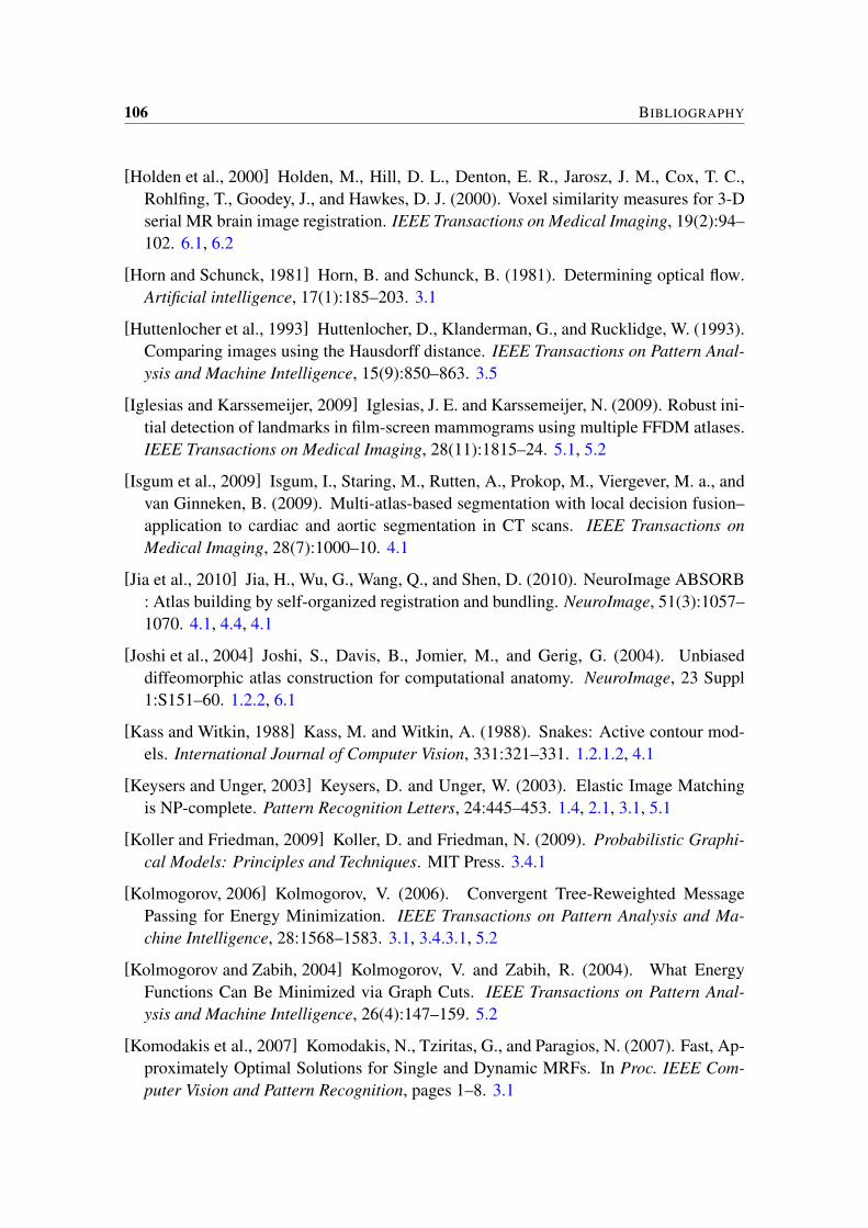
106 BIBLIOGRAPHY
[Holden et al., 2000] Holden, M., Hill, D. L., Denton, E. R., Jarosz, J. M., Cox, T. C.,Rohlfing, T., Goodey, J., and Hawkes, D. J. (2000). Voxel similarity measures for 3-Dserial MR brain image registration. IEEE Transactions on Medical Imaging, 19(2):94–102. 6.1, 6.2
[Horn and Schunck, 1981] Horn, B. and Schunck, B. (1981). Determining optical flow.Artificial intelligence, 17(1):185–203. 3.1
[Huttenlocher et al., 1993] Huttenlocher, D., Klanderman, G., and Rucklidge, W. (1993).Comparing images using the Hausdorff distance. IEEE Transactions on Pattern Anal-ysis and Machine Intelligence, 15(9):850–863. 3.5
[Iglesias and Karssemeijer, 2009] Iglesias, J. E. and Karssemeijer, N. (2009). Robust ini-tial detection of landmarks in film-screen mammograms using multiple FFDM atlases.IEEE Transactions on Medical Imaging, 28(11):1815–24. 5.1, 5.2
[Isgum et al., 2009] Isgum, I., Staring, M., Rutten, A., Prokop, M., Viergever, M. a., andvan Ginneken, B. (2009). Multi-atlas-based segmentation with local decision fusion–application to cardiac and aortic segmentation in CT scans. IEEE Transactions onMedical Imaging, 28(7):1000–10. 4.1
[Jia et al., 2010] Jia, H., Wu, G., Wang, Q., and Shen, D. (2010). NeuroImage ABSORB: Atlas building by self-organized registration and bundling. NeuroImage, 51(3):1057–1070. 4.1, 4.4, 4.1
[Joshi et al., 2004] Joshi, S., Davis, B., Jomier, M., and Gerig, G. (2004). Unbiaseddiffeomorphic atlas construction for computational anatomy. NeuroImage, 23 Suppl1:S151–60. 1.2.2, 6.1
[Kass and Witkin, 1988] Kass, M. and Witkin, A. (1988). Snakes: Active contour mod-els. International Journal of Computer Vision, 331:321–331. 1.2.1.2, 4.1
[Keysers and Unger, 2003] Keysers, D. and Unger, W. (2003). Elastic Image Matchingis NP-complete. Pattern Recognition Letters, 24:445–453. 1.4, 2.1, 3.1, 5.1
[Koller and Friedman, 2009] Koller, D. and Friedman, N. (2009). Probabilistic Graphi-cal Models: Principles and Techniques. MIT Press. 3.4.1
[Kolmogorov, 2006] Kolmogorov, V. (2006). Convergent Tree-Reweighted MessagePassing for Energy Minimization. IEEE Transactions on Pattern Analysis and Ma-chine Intelligence, 28:1568–1583. 3.1, 3.4.3.1, 5.2
[Kolmogorov and Zabih, 2004] Kolmogorov, V. and Zabih, R. (2004). What EnergyFunctions Can Be Minimized via Graph Cuts. IEEE Transactions on Pattern Anal-ysis and Machine Intelligence, 26(4):147–159. 5.2
[Komodakis et al., 2007] Komodakis, N., Tziritas, G., and Paragios, N. (2007). Fast, Ap-proximately Optimal Solutions for Single and Dynamic MRFs. In Proc. IEEE Com-puter Vision and Pattern Recognition, pages 1–8. 3.1
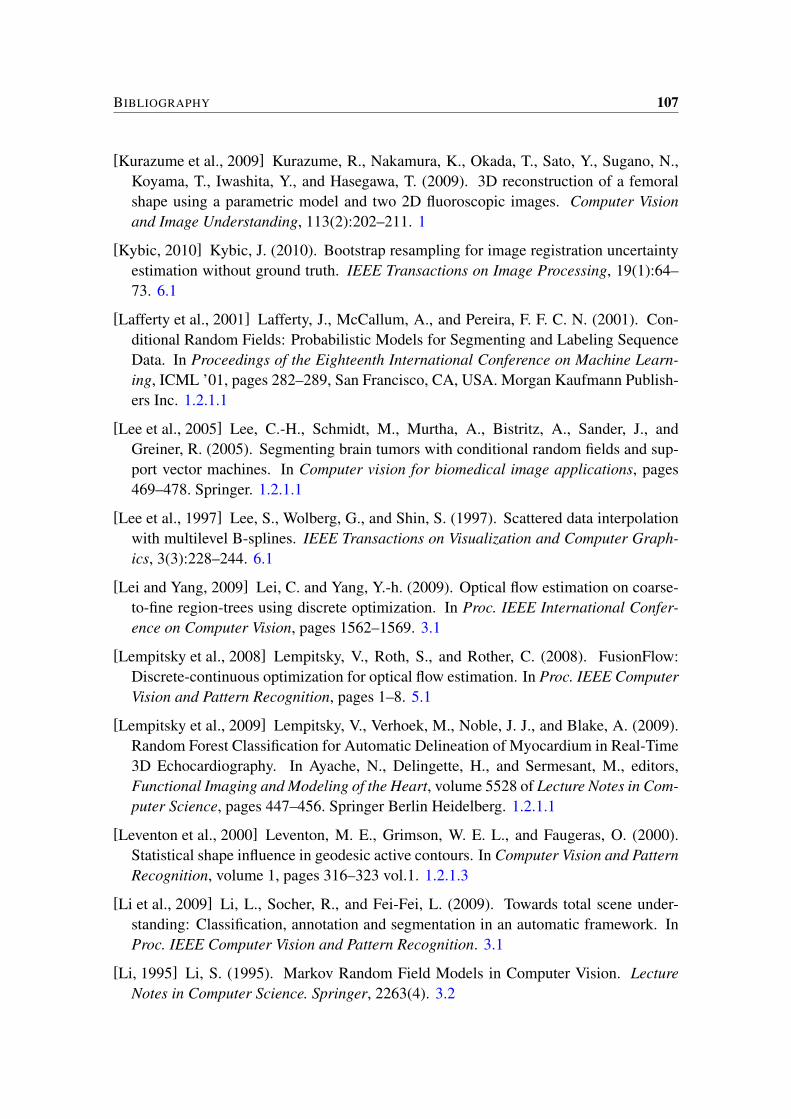
BIBLIOGRAPHY 107
[Kurazume et al., 2009] Kurazume, R., Nakamura, K., Okada, T., Sato, Y., Sugano, N.,Koyama, T., Iwashita, Y., and Hasegawa, T. (2009). 3D reconstruction of a femoralshape using a parametric model and two 2D fluoroscopic images. Computer Visionand Image Understanding, 113(2):202–211. 1
[Kybic, 2010] Kybic, J. (2010). Bootstrap resampling for image registration uncertaintyestimation without ground truth. IEEE Transactions on Image Processing, 19(1):64–73. 6.1
[Lafferty et al., 2001] Lafferty, J., McCallum, A., and Pereira, F. F. C. N. (2001). Con-ditional Random Fields: Probabilistic Models for Segmenting and Labeling SequenceData. In Proceedings of the Eighteenth International Conference on Machine Learn-ing, ICML ’01, pages 282–289, San Francisco, CA, USA. Morgan Kaufmann Publish-ers Inc. 1.2.1.1
[Lee et al., 2005] Lee, C.-H., Schmidt, M., Murtha, A., Bistritz, A., Sander, J., andGreiner, R. (2005). Segmenting brain tumors with conditional random fields and sup-port vector machines. In Computer vision for biomedical image applications, pages469–478. Springer. 1.2.1.1
[Lee et al., 1997] Lee, S., Wolberg, G., and Shin, S. (1997). Scattered data interpolationwith multilevel B-splines. IEEE Transactions on Visualization and Computer Graph-ics, 3(3):228–244. 6.1
[Lei and Yang, 2009] Lei, C. and Yang, Y.-h. (2009). Optical flow estimation on coarse-to-fine region-trees using discrete optimization. In Proc. IEEE International Confer-ence on Computer Vision, pages 1562–1569. 3.1
[Lempitsky et al., 2008] Lempitsky, V., Roth, S., and Rother, C. (2008). FusionFlow:Discrete-continuous optimization for optical flow estimation. In Proc. IEEE ComputerVision and Pattern Recognition, pages 1–8. 5.1
[Lempitsky et al., 2009] Lempitsky, V., Verhoek, M., Noble, J. J., and Blake, A. (2009).Random Forest Classification for Automatic Delineation of Myocardium in Real-Time3D Echocardiography. In Ayache, N., Delingette, H., and Sermesant, M., editors,Functional Imaging and Modeling of the Heart, volume 5528 of Lecture Notes in Com-puter Science, pages 447–456. Springer Berlin Heidelberg. 1.2.1.1
[Leventon et al., 2000] Leventon, M. E., Grimson, W. E. L., and Faugeras, O. (2000).Statistical shape influence in geodesic active contours. In Computer Vision and PatternRecognition, volume 1, pages 316–323 vol.1. 1.2.1.3
[Li et al., 2009] Li, L., Socher, R., and Fei-Fei, L. (2009). Towards total scene under-standing: Classification, annotation and segmentation in an automatic framework. InProc. IEEE Computer Vision and Pattern Recognition. 3.1
[Li, 1995] Li, S. (1995). Markov Random Field Models in Computer Vision. LectureNotes in Computer Science. Springer, 2263(4). 3.2

108 BIBLIOGRAPHY
[Lotfi et al., 2013] Lotfi, T., Tang, L., Andrews, S., and Hamarneh, G. (2013). ImprovingProbabilistic Image Registration via Reinforcement Learning and Uncertainty Evalu-ation. In Wu, G., Zhang, D., Shen, D., Yan, P., Suzuki, K., and Wang, F., editors,Machine Learning in Medical Imaging, volume 8184 of Lecture Notes in ComputerScience, pages 187–194. Springer International Publishing. 6.1
[Lu and Duncan, 2012] Lu, C. and Duncan, J. (2012). A coupled segmentation and reg-istration framework for medical image analysis using robust point matching and activeshape model. In Mathematical Methods in Biomedical Image Analysis, pages 129–136.3.1
[Mahapatra and Sun, 2010] Mahapatra, D. and Sun, Y. (2010). MRF based joint registra-tion and segmentation of dynamic renal MR images. In Proc. SPIE Medical Imaging,pages 754617–6. 3.1
[Mahapatra and Sun, 2012] Mahapatra, D. and Sun, Y. (2012). Integrating segmentationinformation for improved MRF-based elastic image registration. IEEE Transactionson Image Processing, pages 1–13. 1.2.2, 3.1, 3.6
[Majeed et al., 2012] Majeed, T., Fundana, K., Luthi, M., Kiriyanthan, S., Beinemann,J., and Cattin, P. C. (2012). Using a flexibility constrained 3D statistical shape modelfor robust MRF-based segmentation. IEEE Workshop on Mathematical Methods inBiomedical Image Analysis, pages 57–64. 1.2.1.3
[McInerney and Terzopoulos, 1999] McInerney, T. and Terzopoulos, D. (1999). Topol-ogy adaptive deformable surfaces for medical image volume segmentation. IEEETransactions on Medical Imaging, 18(10):840–50. 1.1
[Miller et al., 1993] Miller, M. I., Christensen, G. E., Amit, Y., and Grenander, U. (1993).Mathematical textbook of deformable neuroanatomies. Proceedings of the NationalAcademy of Sciences, 90(24):11944–11948. 1.2.1.2
[Muenzing et al., 2012a] Muenzing, S., Ginneken, B. V., Viergever, M. A., and Pluim, J.P. W. (2012a). DIRBoost: An algorithm for boosting deformable image registration.In International Symposium on Biomedical Imaging, pages 1339–1342. 6.1
[Muenzing et al., 2012b] Muenzing, S. E. A., van Ginneken, B., Murphy, K., and Pluim,J. P. W. (2012b). Supervised quality assessment of medical image registration: appli-cation to intra-patient CT lung registration. Medical image analysis, 16(8):1521–31.6.1
[Myronenko, 2013] Myronenko, A. (2013). Groupwise Image Registration,https://sites.google.com/site/myronenko/software. 5.3, 6.4.3
[Myronenko and Song, 2010] Myronenko, A. and Song, X. (2010). Intensity-based im-age registration by minimizing residual complexity. IEEE Transactions on MedicalImaging, 29(11):1882–1891. 5.3, 6.4.3
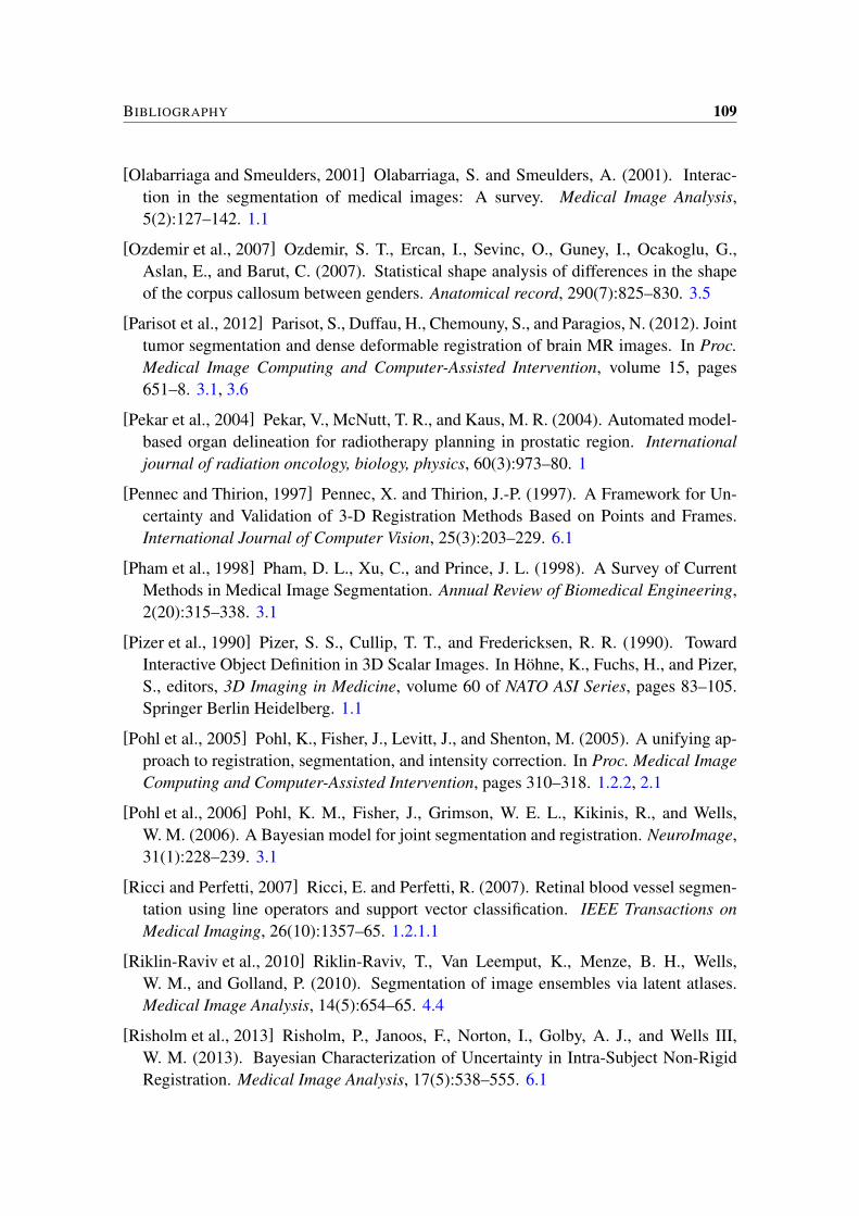
BIBLIOGRAPHY 109
[Olabarriaga and Smeulders, 2001] Olabarriaga, S. and Smeulders, A. (2001). Interac-tion in the segmentation of medical images: A survey. Medical Image Analysis,5(2):127–142. 1.1
[Ozdemir et al., 2007] Ozdemir, S. T., Ercan, I., Sevinc, O., Guney, I., Ocakoglu, G.,Aslan, E., and Barut, C. (2007). Statistical shape analysis of differences in the shapeof the corpus callosum between genders. Anatomical record, 290(7):825–830. 3.5
[Parisot et al., 2012] Parisot, S., Duffau, H., Chemouny, S., and Paragios, N. (2012). Jointtumor segmentation and dense deformable registration of brain MR images. In Proc.Medical Image Computing and Computer-Assisted Intervention, volume 15, pages651–8. 3.1, 3.6
[Pekar et al., 2004] Pekar, V., McNutt, T. R., and Kaus, M. R. (2004). Automated model-based organ delineation for radiotherapy planning in prostatic region. Internationaljournal of radiation oncology, biology, physics, 60(3):973–80. 1
[Pennec and Thirion, 1997] Pennec, X. and Thirion, J.-P. (1997). A Framework for Un-certainty and Validation of 3-D Registration Methods Based on Points and Frames.International Journal of Computer Vision, 25(3):203–229. 6.1
[Pham et al., 1998] Pham, D. L., Xu, C., and Prince, J. L. (1998). A Survey of CurrentMethods in Medical Image Segmentation. Annual Review of Biomedical Engineering,2(20):315–338. 3.1
[Pizer et al., 1990] Pizer, S. S., Cullip, T. T., and Fredericksen, R. R. (1990). TowardInteractive Object Definition in 3D Scalar Images. In Höhne, K., Fuchs, H., and Pizer,S., editors, 3D Imaging in Medicine, volume 60 of NATO ASI Series, pages 83–105.Springer Berlin Heidelberg. 1.1
[Pohl et al., 2005] Pohl, K., Fisher, J., Levitt, J., and Shenton, M. (2005). A unifying ap-proach to registration, segmentation, and intensity correction. In Proc. Medical ImageComputing and Computer-Assisted Intervention, pages 310–318. 1.2.2, 2.1
[Pohl et al., 2006] Pohl, K. M., Fisher, J., Grimson, W. E. L., Kikinis, R., and Wells,W. M. (2006). A Bayesian model for joint segmentation and registration. NeuroImage,31(1):228–239. 3.1
[Ricci and Perfetti, 2007] Ricci, E. and Perfetti, R. (2007). Retinal blood vessel segmen-tation using line operators and support vector classification. IEEE Transactions onMedical Imaging, 26(10):1357–65. 1.2.1.1
[Riklin-Raviv et al., 2010] Riklin-Raviv, T., Van Leemput, K., Menze, B. H., Wells,W. M., and Golland, P. (2010). Segmentation of image ensembles via latent atlases.Medical Image Analysis, 14(5):654–65. 4.4
[Risholm et al., 2013] Risholm, P., Janoos, F., Norton, I., Golby, A. J., and Wells III,W. M. (2013). Bayesian Characterization of Uncertainty in Intra-Subject Non-RigidRegistration. Medical Image Analysis, 17(5):538–555. 6.1
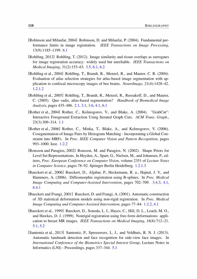
110 BIBLIOGRAPHY
[Robinson and Milanfar, 2004] Robinson, D. and Milanfar, P. (2004). Fundamental per-formance limits in image registration. IEEE Transactions on Image Processing,13(9):1185–1199. 6.1
[Rohlfing, 2012] Rohlfing, T. (2012). Image similarity and tissue overlaps as surrogatesfor image registration accuracy: widely used but unreliable. IEEE Transactions onMedical Imaging, 31(2):153–63. 3.5, 6.1, 6.2
[Rohlfing et al., 2004] Rohlfing, T., Brandt, R., Menzel, R., and Maurer, C. R. (2004).Evaluation of atlas selection strategies for atlas-based image segmentation with ap-plication to confocal microscopy images of bee brains. NeuroImage, 21(4):1428–42.1.2.1.2
[Rohlfing et al., 2005] Rohlfing, T., Brandt, R., Menzel, R., Russakoff, D., and Maurer,C. (2005). Quo vadis, atlas-based segmentation? Handbook of Biomedical ImageAnalysis, pages 435–486. 2.1, 3.1, 3.6, 4.1, 6.1
[Rother et al., 2004] Rother, C., Kolmogorov, V., and Blake, A. (2004). "GrabCut":Interactive Foreground Extraction Using Iterated Graph Cuts. ACM Trans. Graph.,23(3):309–314. 1.1
[Rother et al., 2006] Rother, C., Minka, T., Blake, A., and Kolmogorov, V. (2006).Cosegmentation of Image Pairs by Histogram Matching - Incorporating a Global Con-straint into MRFs. In Proc. IEEE Computer Vision and Pattern Recognition, pages993–1000. Ieee. 1.2.2
[Rousson and Paragios, 2002] Rousson, M. and Paragios, N. (2002). Shape Priors forLevel Set Representations. In Heyden, A., Sparr, G., Nielsen, M., and Johansen, P., ed-itors, Proc. European Conference on Computer Vision, volume 2351 of Lecture Notesin Computer Science, pages 78–92. Springer Berlin Heidelberg. 1.2.1.3
[Rueckert et al., 2006] Rueckert, D., Aljabar, P., Heckemann, R. a., Hajnal, J. V., andHammers, A. (2006). Diffeomorphic registration using B-splines. In Proc. MedicalImage Computing and Computer-Assisted Intervention, pages 702–709. 3.4.3, 4.1,6.4.1
[Rueckert and Frangi, 2001] Rueckert, D. and Frangi, A. (2001). Automatic constructionof 3D statistical deformation models using non-rigid registration. In Proc. MedicalImage Computing and Computer-Assisted Intervention, pages 77–84. 1.2.2, 4.1
[Rueckert et al., 1999] Rueckert, D., Sonoda, L. I., Hayes, C., Hill, D. L., Leach, M. O.,and Hawkes, D. J. (1999). Nonrigid registration using free-form deformations: appli-cation to breast MR images. IEEE Transactions on Medical Imaging, 18(8):712–21.5.1, 5.2
[Santemiz et al., 2013] Santemiz, P., Spreeuwers, L. J., and Veldhuis, R. N. J. (2013).Automatic landmark detection and face recognition for side-view face images. InInternational Conference of the Biometrics Special Interest Group, Lecture Notes inInformatics (LNI) - Proceedings, pages 337–344. 5.1
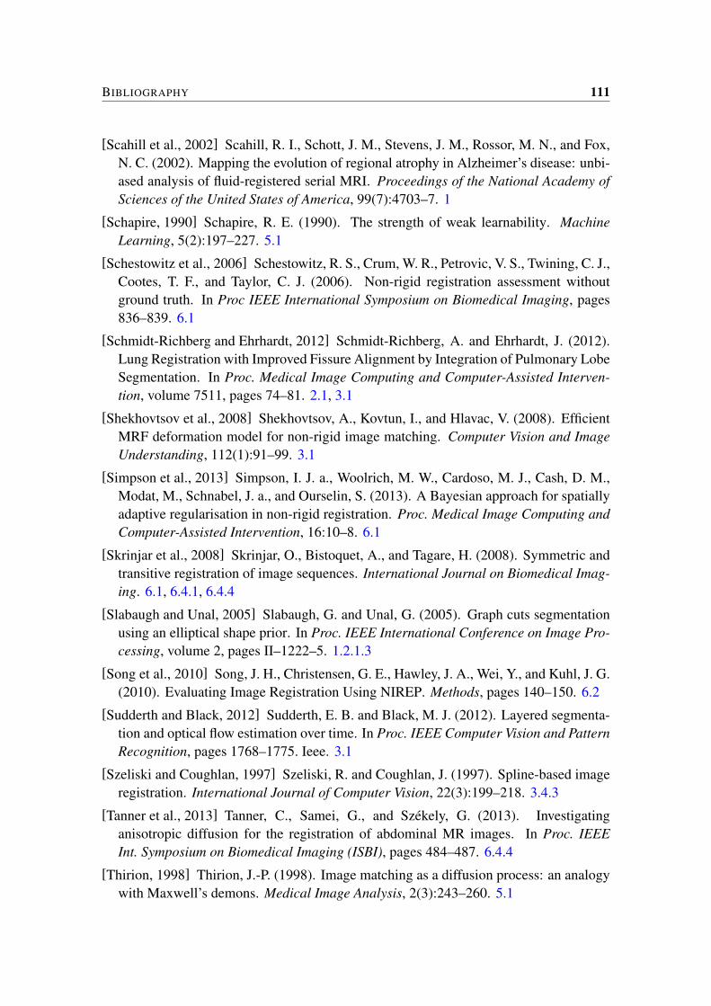
BIBLIOGRAPHY 111
[Scahill et al., 2002] Scahill, R. I., Schott, J. M., Stevens, J. M., Rossor, M. N., and Fox,N. C. (2002). Mapping the evolution of regional atrophy in Alzheimer’s disease: unbi-ased analysis of fluid-registered serial MRI. Proceedings of the National Academy ofSciences of the United States of America, 99(7):4703–7. 1
[Schapire, 1990] Schapire, R. E. (1990). The strength of weak learnability. MachineLearning, 5(2):197–227. 5.1
[Schestowitz et al., 2006] Schestowitz, R. S., Crum, W. R., Petrovic, V. S., Twining, C. J.,Cootes, T. F., and Taylor, C. J. (2006). Non-rigid registration assessment withoutground truth. In Proc IEEE International Symposium on Biomedical Imaging, pages836–839. 6.1
[Schmidt-Richberg and Ehrhardt, 2012] Schmidt-Richberg, A. and Ehrhardt, J. (2012).Lung Registration with Improved Fissure Alignment by Integration of Pulmonary LobeSegmentation. In Proc. Medical Image Computing and Computer-Assisted Interven-tion, volume 7511, pages 74–81. 2.1, 3.1
[Shekhovtsov et al., 2008] Shekhovtsov, A., Kovtun, I., and Hlavac, V. (2008). EfficientMRF deformation model for non-rigid image matching. Computer Vision and ImageUnderstanding, 112(1):91–99. 3.1
[Simpson et al., 2013] Simpson, I. J. a., Woolrich, M. W., Cardoso, M. J., Cash, D. M.,Modat, M., Schnabel, J. a., and Ourselin, S. (2013). A Bayesian approach for spatiallyadaptive regularisation in non-rigid registration. Proc. Medical Image Computing andComputer-Assisted Intervention, 16:10–8. 6.1
[Skrinjar et al., 2008] Skrinjar, O., Bistoquet, A., and Tagare, H. (2008). Symmetric andtransitive registration of image sequences. International Journal on Biomedical Imag-ing. 6.1, 6.4.1, 6.4.4
[Slabaugh and Unal, 2005] Slabaugh, G. and Unal, G. (2005). Graph cuts segmentationusing an elliptical shape prior. In Proc. IEEE International Conference on Image Pro-cessing, volume 2, pages II–1222–5. 1.2.1.3
[Song et al., 2010] Song, J. H., Christensen, G. E., Hawley, J. A., Wei, Y., and Kuhl, J. G.(2010). Evaluating Image Registration Using NIREP. Methods, pages 140–150. 6.2
[Sudderth and Black, 2012] Sudderth, E. B. and Black, M. J. (2012). Layered segmenta-tion and optical flow estimation over time. In Proc. IEEE Computer Vision and PatternRecognition, pages 1768–1775. Ieee. 3.1
[Szeliski and Coughlan, 1997] Szeliski, R. and Coughlan, J. (1997). Spline-based imageregistration. International Journal of Computer Vision, 22(3):199–218. 3.4.3
[Tanner et al., 2013] Tanner, C., Samei, G., and Székely, G. (2013). Investigatinganisotropic diffusion for the registration of abdominal MR images. In Proc. IEEEInt. Symposium on Biomedical Imaging (ISBI), pages 484–487. 6.4.4
[Thirion, 1998] Thirion, J.-P. (1998). Image matching as a diffusion process: an analogywith Maxwell’s demons. Medical Image Analysis, 2(3):243–260. 5.1
112 BIBLIOGRAPHY
[Udupa, 1997] Udupa, J. K. (1997). Multiple sclerosis lesion quantification using fuzzy-connectedness principles. IEEE Transactions on Medical Imaging, 16(5):598–609.1.1
[van Rikxoort et al., 2010] van Rikxoort, E. M., Isgum, I., Arzhaeva, Y., Staring, M.,Klein, S., Viergever, M. a., Pluim, J. P. W., and van Ginneken, B. (2010). Adaptive localmulti-atlas segmentation: application to the heart and the caudate nucleus. MedicalImage Analysis, 14(1):39–49. 4.1
[Veksler, 2008] Veksler, O. (2008). Star shape prior for graph-cut image segmentation.In European Conference on Computer Vision, pages 454–467. 1.2.1.3
[Veksler and Delong, 2013] Veksler, O. and Delong, A. (2013). Multi-Label Optimiza-tion using Graph-Cuts, http://vision.csd.uwo.ca/code/. 3.4.3.1
[Vercauteren et al., 2008] Vercauteren, T., Pennec, X., Perchant, A., and Ayache, N.(2008). Symmetric log-domain diffeomorphic Registration: a demons-based approach.In Proc. Medical Image Computing and Computer-Assisted Intervention, pages 754–61. 5.1, 6.1
[Vercauteren et al., 2009] Vercauteren, T., Pennec, X., Perchant, A., and Ayache, N.(2009). Diffeomorphic demons: efficient non-parametric image registration. Neu-roImage, 45(1 Suppl):61–72. 3.5, 3.5, 5.1, 5.3, 6.4.2
[Vishnevskiy et al., 2014] Vishnevskiy, V., Gass, T., Székely, G., and Goksel, O. (2014).Total Variation Regularization of Displacements in Parametric Image Registration. InProc. MICCAI Workshop on Abdominal Imaging, volume 8676 of Lecture Note inComputer Science (LNCS), page in press. 6.4.4
[von Siebenthal et al., 2007] von Siebenthal, M., Székely, G., Gamper, U., Boesiger, P.,Lomax, A., and Cattin, P. (2007). 4D MR imaging of respiratory organ motion and itsvariability. Physics in medicine and biology, 52(6):1547–64. 6.4.4
[Wang et al., 2006a] Wang, F., Vemuri, B. C., and Eisenschenk, S. J. (2006a). Joint reg-istration and segmentation of neuroanatomic structures from brain MRI. Academicradiology, 13(9):1104–11. 3.1
[Wang et al., 2006b] Wang, F., Wang, J., Zhang, C., Shen, H. C., Bay, C. W., and Kong,H. (2006b). Semi-Supervised Classification Using Linear Neighborhood Propagation.Science And Technology. 4.1
[Warfield et al., 2004] Warfield, S., Zou, K., and Wells, W. M. (2004). Simultaneoustruth and performance level estimation (STAPLE): an algorithm for the validation ofimage segmentation. IEEE Transactions on Medical Imaging, 23(7):903–921. 1.2.1.2
[Woods et al., 1998] Woods, R. P., Grafton, S. T., Holmes, C. J., Cherry, S. R., and Mazz-iotta, J. C. (1998). Automated image registration: I. General methods and intrasubject,intramodality validation. Journal of Computer Assisted Tomography, 22(1):139–52.6.1, 6.2

BIBLIOGRAPHY 113
[Wyatt and Noble, 2003] Wyatt, P. and Noble, J. (2003). MAP MRF joint segmentationand registration of medical images. Medical Image Analysis, 7(4):539–552. 1.2.2, 2.1,2.2.1, 3.1, 3.2
[Xiaohua et al., 2004] Xiaohua, C., Brady, M., and Rueckert, D. (2004). Simultaneoussegmentation and registration for medical image. In Proc. Medical Image Computingand Computer-Assisted Intervention, pages 663–670. 2.1, 3.1
[Yamamoto et al., 1999] Yamamoto, M., Nagata, Y., Okajima, K., Ishigaki, T., Murata,R., Mizowaki, T., Kokubo, M., and Hiraoka, M. (1999). Differences in target out-line delineation from CT scans of brain tumours using different methods and differentobservers. Radiotherapy and Oncology, 50(2):151–156. 1.1
[Zachow et al., 2005] Zachow, S., Lamecker, H., Elsholtz, B., and Stiller, M. (2005).Reconstruction of mandibular dysplasia using a statistical 3D shape model. In Pro-ceedings of the 19th International Congress and Exhibition on Computer Assisted Ra-diology and Surgery, volume 1281, pages 1238–1243. 1
[Zhu and Ghahramani, 2002] Zhu, X. and Ghahramani, Z. (2002). Learning from labeledand unlabeled data with label propagation. Technical report, School Comput. Sci.,Carnegie Mellon Univ. 4.1