measuring urban sprawl and validating sprawl measures · metropolitan counties or statistically...
TRANSCRIPT
1
Abstract
Across the nation, the debate over metropolitan sprawl and its impacts continues. A decade ago, Smart
Growth America (SGA) and the U.S. Environmental Protection Agency (EPA) sought to raise the level of
this debate by sponsoring groundbreaking research on sprawl and its quality-of-life consequences
(Ewing et al. 2002; Ewing et al. 2003a, 2003b, 2003c). The original sprawl indices were made available to
researchers who wished to explore the various costs and benefits of sprawl. They have been widely used
in outcome-related research, particularly in connection with public health. Sprawl has been linked to
physical inactivity, obesity, traffic fatalities, poor air quality, residential energy use, emergency response
times, teenage driving, lack of social capital, and private-vehicle commute distances and times (Ewing et
al. 2003a; Ewing et al. 2003b; Ewing et al. 2003c; Kelly-Schwartz et al. 2004; Sturm and Cohen 2004; Cho
et al. 2006; Doyle et al. 2006; Ewing et al. 2006; Kahn 2006; Kim et al. 2006; Plantinga and Bernell 2007;
Ewing and Rong 2008; Joshu et al. 2008; Stone 2008; Trowbridge and McDonald 2008; Fan and Song
2009; McDonald and Trowbridge 2009; Trowbridge et al. 2009; Lee et al. 2009; Nguyen 2010; Stone et
al. 2010; Schweitzer and Zhou 2010; Zolnik 2011; Holcombe and Williams 2012; Griffin et al. 2013;
Bereitschaft and Debbage 2013).
In this study for the National Cancer Institute, the Brookings Institution, and Smart Growth America, we
begin in Chapter 1 by updating the original county indices to 2010. As one would expect, the degree of
county sprawl does not change dramatically over a 10-year period. Also, given their fixed boundaries,
most counties become more compact (denser and with smaller blocks) over the 10-year period. Sprawl
occurs mainly as previously rural counties (in 2000) outside metropolitan areas become low density
suburbs and exurbs of metropolitan areas (in 2010).
In Chapter 2, we develop refined versions of the indices that incorporate more measures of the built
environment. The refined indices capture four distinct dimensions of sprawl, thereby characterizing
county sprawl in all its complexity. The four are development density, land use mix, population and
employment centering, and street accessibility. The dimensions of the new county indices parallel the
metropolitan indices developed by Ewing et al. (2002), basically representing the relative accessibility
provided by the county. The simple structure of the original county sprawl index has become more
complex, but also more nuanced and comprehensive, in line with definitions of sprawl in the technical
literature.
In Chapter 3, we develop metropolitan sprawl indices that, like the refined county indices, have four
distinct dimensions-- development density, land use mix, population and employment centering, and
street accessibility. Compared to metropolitan sprawl indices from the early 2000s, these new indices

2
incorporate more variables and hence have more construct validity. For example, the earlier effort
defined density strictly in terms of population concentrations, while this effort considers employment
concentrations as well. The reason for developing metropolitan sprawl indices, rather than limiting
ourselves to counties, is that metropolitan areas are natural units of analysis for certain quality-of-life
outcomes.
In Chapter 4, we conduct one of the first longitudinal analysis of sprawl to see which areas are sprawling
more over time, and which are sprawling less or actually becoming more compact. To conduct such as
analysis, we need to employ a new level of geography, the census urbanized area. In contrast of
counties and metropolitan areas, urbanized areas expand incrementally as areas grow and rural tracts
are converted to urban and suburban uses. The analysis shows that, on average, urban sprawl in the U.S.
increased between 2000 and 2010, but that there are many exceptions to this generalization.
Finally, in chapter 5, we develop compactness indices for census tracts within metropolitan areas. We
know from the travel and public health literatures that there is a demand in the research community for
built environmental metrics at the sub-county level, what might be described as the community or
neighborhood scale.
The appendices provide values of compactness/sprawl indices for census tracts, counties, metropolitan
areas, and urbanized areas. Data are available in electronic form at http://gis.cancer.gov/tools/urban-
sprawl/
3
Table of Contents Abstract ......................................................................................................................................................... 1
Chapter 1. Updated County Sprawl Index .................................................................................................... 5
Update to 2010 ......................................................................................................................................... 7
Chapter 2. Refined County Sprawl Measures ............................................................................................. 11
Density .................................................................................................................................................... 11
Mixed Use ............................................................................................................................................... 12
Centering ................................................................................................................................................. 14
Street Accessibility .................................................................................................................................. 17
Relationship Among Compactness Factors ............................................................................................. 18
Composite Index ..................................................................................................................................... 18
Greater Validity of New Index ................................................................................................................. 20
Chapter 3. Derivation of Metropolitan Sprawl Indices ............................................................................... 25
Methods .................................................................................................................................................. 25
Sample ........................................................................................................................................... 25
Variables ........................................................................................................................................ 26
Results ..................................................................................................................................................... 28
Individual Compactness/Sprawl Factors ........................................................................................ 28
Overall Compactness/Sprawl Index for 2010 ................................................................................ 30
Discussion................................................................................................................................................ 32
Chapter 4. Urbanized Areas: A Longitudinal Analysis ................................................................................. 79
Methods .................................................................................................................................................. 79
Sample ........................................................................................................................................... 79
Variables ........................................................................................................................................ 79
Results ..................................................................................................................................................... 82
Individual Compactness/Sprawl Factors ........................................................................................ 82
Overall Compactness/Sprawl Index for 2010 ................................................................................ 83
Overall Compactness/Sprawl Index for 2000 ................................................................................ 84
Discussion................................................................................................................................................ 85
Chapter 5. Derivation of Census Tract Sprawl Indices ................................................................................ 86
Chapter 6. Conclusion ................................................................................................................................. 87
References .................................................................................................................................................. 88
4
Appendix A. County Compactness Indices for 2010, 2000, and Changes .................................................. 91
Appendix B. County Compactness Factors and Composite Indices for 2010 .......................................... 115
Appendix C. 2010 Metropolitan Indices ................................................................................................... 141
Appendix D. Urbanized Areas Compactness Indices 2010 ....................................................................... 149
Appendix E. Urbanized Areas Compactness Indices 2000 ........................................................................ 154
5
Chapter 1. Updated County Sprawl Index
Ewing et al. (2003b; 2003c) originally estimated a single county sprawl index for each of 448
metropolitan counties or statistically equivalent entities (e.g., independent towns and cities). These
counties comprised the 101 most populous metropolitan statistical areas, consolidated metropolitan
statistical areas, and New England county metropolitan areas in the United States as of the 1990 census,
the latest year for which metropolitan boundaries were defined as that study began. Nonmetropolitan
counties, and metropolitan counties in smaller metropolitan areas, were excluded from the sample.
More than 183 million Americans, nearly two-thirds of the United States population, lived in these 448
counties in 2000.
Six variables were part of the original county sprawl index (as shown in Table 1). U.S. Census data were
used to derive three population density measures for each county:
gross population density in persons per square mile (popden)
percentage of the county population living at low suburban densities, specifically, densities
between 100 and 1,500 persons per square mile, corresponding to less than one housing unit
per acre (lt1500)
percentage of the county population living at medium to high urban densities, specifically, more
than 12,500 persons per square mile, corresponding to about 8 housing units per acre, the lower
limit of density needed to support mass transit (gt12500)
In deriving population density measures, census tracts were excluded if they had fewer than 100
residents per square mile (corresponding to rural areas, desert tracts, and other undeveloped lands).
Ewing et al. were only concerned with sprawl in developed areas where the vast majority of residents
live.
A fourth density variable was derived from estimated urban land area for each county from the National
Resources Inventory of the U.S. Department of Agriculture.
net population density of urban places within the county (urbden)
Data reflecting street accessibility for each county were also obtained from the U.S. Census. Street
accessibility is related to block size since smaller blocks translate into shorter and more direct routes. A
census block is defined as a statistical area bounded on all sides by streets, roads, streams, railroad
tracks, or geopolitical boundary lines, in most cases. A traditional urban neighborhood is composed of
intersecting bounding streets that form a grid, with houses built on the four sides of the block, facing
these streets. The length of each side of that block, and therefore its block size, is relatively small. By
contrast, a contemporary suburban neighborhood does not make connections between adjacent cul-de-
sacs or loop roads. Instead, local streets only connect with the street at the subdivision entrance, which
is on one side of the block boundary. Thus, the length of a side of this block is quite large, and the block
itself often encloses multiple subdivisions to form a superblock, a half mile or more on a side. Large
block sizes indicate a relative paucity of street connections and alternate routes.
6
Two street accessibility variables were computed for each county:
average block size (avgblk)
percentage of blocks with areas less than 1/100 square mile, the size of a typical traditional
urban block bounded by sides just over 500 feet in length (smlblk).
Blocks larger than one square mile were excluded from these calculations, since they were likely to be in
rural or other undeveloped areas.
The six variables were combined into one factor representing the degree of sprawl within the county.
This was accomplished via principal component analysis, an analytical technique that takes a large
number of correlated variables and extracts a small number of factors that embody the common
variance in the original data set. The extracted factors, or principal components, are weighted
combinations of the original variables. When a variable is given a great deal of weight in constructing a
principal component, we say that the variable loads heavily on that component. The greater the
correlation between an original variable and a principal component, the greater the loading and the
more weight the original variable is given in the overall principal component score. The more highly
correlated the original variables, the more variance is captured by a single principal component.
The principal component selected to represent sprawl was the one capturing the largest share of
common variance among the six variables, that is, the one upon which the observed variables loaded
most heavily. This one component accounted for almost two-thirds of the variance in the dataset.
Because this component captured the majority of the combined variance of these variables, no
subsequent components were considered.
To arrive at a final index, Ewing et al. transformed the principal component, which had a mean of 0 and
standard deviation of 1, to a scale with a mean of 100 and standard deviation of 25. This transformation
produced a more familiar metric (like an IQ scale) and ensured that all values would be positive, thereby
allowing us to take natural logarithms and estimate elasticities.
The bigger the value of the index, the more compact the county. The smaller the value, the more
sprawling the county. Scores ranged from a high of 352 to a low of 63. At the most compact end of the
scale were four New York City boroughs, Manhattan, Brooklyn, Bronx, and Queens; San Francisco
County; Hudson County (Jersey City); Philadelphia County; and Suffolk County (Boston). At the most
sprawling end of the scale were outlying counties of metropolitan areas in the Southeast and Midwest
such as Goochland County in the Richmond, VA metropolitan area and Geauga County in the Cleveland,
OH metropolitan area. The county sprawl index was positively skewed. Most counties clustered around
intermediate levels of sprawl. In the U.S., few counties approach the densities of New York or San
Francisco.
For these counties, the original sprawl index was validated against journey to work, adult obesity, and
traffic fatality data (Ewing et al. 2003a; Ewing et al. 2003b; Ewing et al. 2003c). Later, the same county
sprawl index was used to model the built environment in a study of youth obesity (Ewing et al. 2006).
For this study, the index was computed for additional counties or county equivalents in order to have
7
sprawl data for more National Longitudinal Survey of Youth (NLSY97) respondents. The 954 counties or
county equivalents in the expanded sample represented the vast majority of counties lying within U.S.
metropolitan areas, as defined by the U.S. Census Bureau in December 2003. Almost 82% of the U.S.
population lived in metropolitan counties for which county sprawl indices were now available. Most
recent research on sprawl and its impacts has made use of this expanded dataset.
Update to 2010
In updating the original county sprawl index to 2010, five of the six variables were derived in the exact
same way as for 1990 and 2000. U.S. Census files for summary levels 140 (census tracts) and 101
(census blocks) were downloaded from American FactFinder. Population data were extracted for all
census tracts in all metropolitan counties. Land area data were extracted for all census blocks in all
metropolitan counties. Ninety-nine metropolitan counties were lost to the sample because they had no
census tracts averaging 100 persons per square mile or more. They were deemed to be rural.
The sixth variable, net density of urban areas within the county, was originally computed using data on
“urban and built up uses” from the National Resources Inventory of the U.S. Department of Agriculture.
The most recent NRI (2007) does not provide data at the county level. Therefore the U.S. Geological
Survey’s National Land Cover Database (NLCD) was used instead. NLCD serves as the definitive Landsat-
based, 30-meter resolution, land cover database for the Nation. It is a raster dataset providing spatial
reference for land surface classification (for example, urban, agriculture, forest). It can be geo-
processed to any geographic unit.
For the current work, the urban land area was generated at the county level using NLCD 2006 (the latest
product) and county geography (2010) for the entire U.S. Using the “Tabulate Area” spatial analyst tool
within ArcGIS, urban land areas within each county were calculated. The noncontiguous areas in the
same county were aggregated resulting in total urban area in square miles. The value codes treated as
urban were:
21. Developed, Open Space - Areas with a mixture of some constructed materials, but mostly
vegetation in the form of lawn grasses. Impervious surfaces account for less than 20% of total
cover. These areas most commonly include large-lot single-family housing units, parks, golf
courses, and vegetation planted in developed settings for recreation, erosion control, or
aesthetic purposes.
22. Developed, Low Intensity - Areas with a mixture of constructed materials and vegetation.
Impervious surfaces account for 20% to 49% percent of total cover. These areas most commonly
include single-family housing units.
23. Developed, Medium Intensity – Areas with a mixture of constructed materials and
vegetation. Impervious surfaces account for 50% to 79% of the total cover. These areas most
commonly include single-family housing units.
8
24. High Intensity - Highly developed areas where people reside or work in high numbers.
Examples include apartment complexes, row houses and commercial/industrial. Impervious
surfaces account for 80% to 100% of the total cover.
The NRI and NLCD datasets are fairly comparable (see Appendix A), making the county sprawl indices for
1990, 2000, and 2010 fairly comparable. However, NLCD is only available for the continental U.S.
Therefore counties and county equivalents from Alaska, Hawaii, and Puerto Rico, 72 in total, were lost to
the sample.
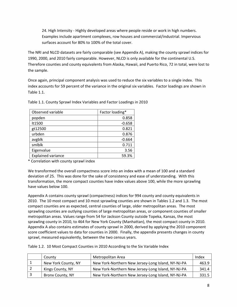
Once again, principal component analysis was used to reduce the six variables to a single index. This
index accounts for 59 percent of the variance in the original six variables. Factor loadings are shown in
Table 1.1.
Table 1.1. County Sprawl Index Variables and Factor Loadings in 2010
Observed variable Factor loading*
popden 0.858
lt1500 -0.658
gt12500 0.821
urbden 0.876
avgblk -0.664
smlblk 0.711
Eigenvalue 3.56
Explained variance 59.3%
* Correlation with county sprawl index
We transformed the overall compactness score into an index with a mean of 100 and a standard deviation of 25. This was done for the sake of consistency and ease of understanding. With this transformation, the more compact counties have index values above 100, while the more sprawling have values below 100.
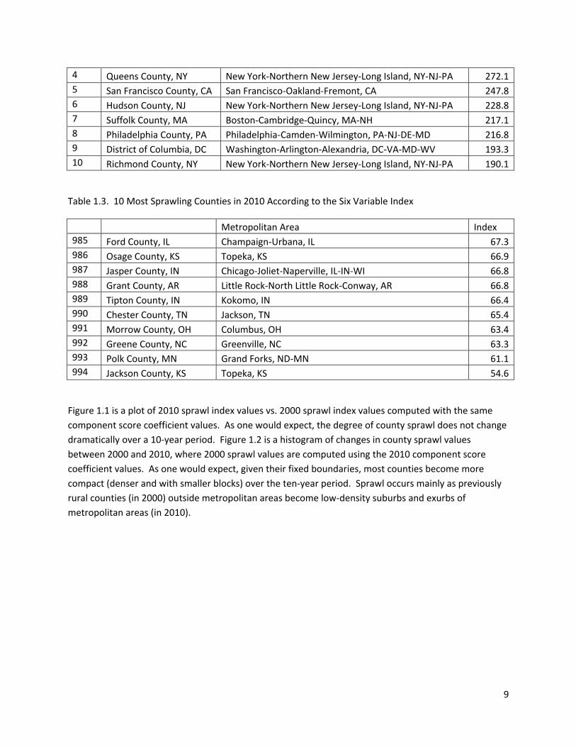
Appendix A contains county sprawl (compactness) indices for 994 county and county equivalents in 2010. The 10 most compact and 10 most sprawling counties are shown in Tables 1.2 and 1.3. The most compact counties are as expected, central counties of large, older metropolitan areas. The most sprawling counties are outlying counties of large metropolitan areas, or component counties of smaller metropolitan areas. Values range from 54 for Jackson County outside Topeka, Kansas, the most sprawling county in 2010, to 464 for New York County (Manhattan), the most compact county in 2010. Appendix A also contains estimates of county sprawl in 2000, derived by applying the 2010 component score coefficient values to data for counties in 2000. Finally, the appendix presents changes in county sprawl, measured equivalently, between the two census years.
Table 1.2. 10 Most Compact Counties in 2010 According to the Six Variable Index
County Metropolitan Area Index
1 New York County, NY New York-Northern New Jersey-Long Island, NY-NJ-PA 463.9
2 Kings County, NY New York-Northern New Jersey-Long Island, NY-NJ-PA 341.4
3 Bronx County, NY New York-Northern New Jersey-Long Island, NY-NJ-PA 331.5
9
4 Queens County, NY New York-Northern New Jersey-Long Island, NY-NJ-PA 272.1
5 San Francisco County, CA San Francisco-Oakland-Fremont, CA 247.8
6 Hudson County, NJ New York-Northern New Jersey-Long Island, NY-NJ-PA 228.8
7 Suffolk County, MA Boston-Cambridge-Quincy, MA-NH 217.1
8 Philadelphia County, PA Philadelphia-Camden-Wilmington, PA-NJ-DE-MD 216.8
9 District of Columbia, DC Washington-Arlington-Alexandria, DC-VA-MD-WV 193.3
10 Richmond County, NY New York-Northern New Jersey-Long Island, NY-NJ-PA 190.1
Table 1.3. 10 Most Sprawling Counties in 2010 According to the Six Variable Index
Metropolitan Area Index
985 Ford County, IL Champaign-Urbana, IL 67.3
986 Osage County, KS Topeka, KS 66.9
987 Jasper County, IN Chicago-Joliet-Naperville, IL-IN-WI 66.8
988 Grant County, AR Little Rock-North Little Rock-Conway, AR 66.8
989 Tipton County, IN Kokomo, IN 66.4
990 Chester County, TN Jackson, TN 65.4
991 Morrow County, OH Columbus, OH 63.4
992 Greene County, NC Greenville, NC 63.3
993 Polk County, MN Grand Forks, ND-MN 61.1
994 Jackson County, KS Topeka, KS 54.6
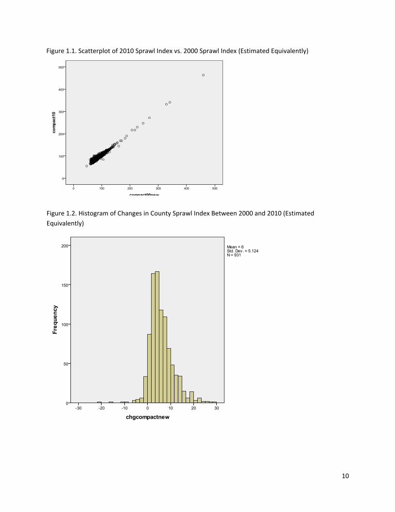
Figure 1.1 is a plot of 2010 sprawl index values vs. 2000 sprawl index values computed with the same
component score coefficient values. As one would expect, the degree of county sprawl does not change
dramatically over a 10-year period. Figure 1.2 is a histogram of changes in county sprawl values
between 2000 and 2010, where 2000 sprawl values are computed using the 2010 component score
coefficient values. As one would expect, given their fixed boundaries, most counties become more
compact (denser and with smaller blocks) over the ten-year period. Sprawl occurs mainly as previously
rural counties (in 2000) outside metropolitan areas become low-density suburbs and exurbs of
metropolitan areas (in 2010).
10
Figure 1.1. Scatterplot of 2010 Sprawl Index vs. 2000 Sprawl Index (Estimated Equivalently)
Figure 1.2. Histogram of Changes in County Sprawl Index Between 2000 and 2010 (Estimated
Equivalently)
11
Chapter 2. Refined County Sprawl Measures
A literature review by Ewing (1997) found poor accessibility to be the common denominator of sprawl.
Sprawl is viewed as any development pattern in which related land uses have poor access to one
another, leaving residents with no alternative to long distance trips by automobile. Compact
development, the polar opposite, is any development pattern in which related land uses are highly
accessible to one another, thus minimizing automobile travel and attendant social, economic, and
environmental costs. The following patterns are most often identified in the literature: scattered or
leapfrog development, commercial strip development, uniform low-density development, or single-use
development (with different land uses segregated from one another, as in bedroom communities). In
scattered or leapfrog development, residents and service providers must pass by vacant land on their
way from one developed use to another. In classic strip development, the consumer must pass other
uses on the way from one store to the next; it is the antithesis of multipurpose travel to an activity
center. Of course, in low-density, single-use development, everything is far apart due to large private
land holdings and segregation of land uses.
While the technical literature on sprawl focuses on land use patterns that produce poor regional
accessibility, poor accessibility is also a product of fragmented street networks that separate urban
activities more than need be. When asked, planners now routinely associate sprawl with sparse street
networks as well as dispersed land use patterns.
The original county sprawl index operationalized only two dimensions of urban form—residential
density and street accessibility. Our grant from the National Institutes of Health (NIH) provides for the
development of refined measures of county compactness or, conversely, county sprawl. These measures
are modeled after the more complete metropolitan sprawl indices developed by Ewing et al. (2002).
The refined indices operationalize four dimensions, thereby characterizing county sprawl in all its
complexity. The four are density, mix, centering, and street accessibility. The dimensions of the new
county indices parallel the metropolitan indices, basically representing the relative accessibility provided
by the county.
The full set of variables was used to derive a refined set of compactness/sprawl factors using principal
component analysis. One principal component represents population density, another land use mix, a
third centering, and a fourth street accessibility. County principal component values, standardized such
that the mean value of each is 100 and the standard deviation is 25, are presented in Appendix B. The
simple structure of the original county sprawl index has become more complex, but also more nuanced
and comprehensive, in line with definitions of sprawl in the technical literature.
Density
Low residential density is on everyone’s list of sprawl indicators. Our first four density variables are the
same as in the original sprawl index, gross density of urban and suburban census tracts (popden),
percentage of the population living at low suburban densities (lt1500), percentage of the population
12
living at medium to high urban densities (gt12500), and urban density based on the National Land Cover
Database (urbden).
The fifth density variable is analogous to the first, except it is derived with employment data from the
Local Employment Dynamics (LED) database rather than population data from the 2010 Census. The LED
database is assembled by the Census Bureau through a voluntary partnership with state labor market
information agencies. The data provide unprecedented details about America's jobs, workers, and local
economies. The LED data, available from 2002 to 2010, are collected at census block geography level
and can be aggregated to any larger geography, in this case block groups. LED variables include total
number of jobs, average age of workers, monthly earnings, and as of 2009 sex, race, ethnicity, and
education levels. In this case, LED data were processed for the year 2010. The data were aggregated
from census block geography to census block group geography to generate total jobs by two-digit NAICS
code for every block group in the nation, except those in Massachusetts, which doesn’t participate in
the program. The density variable derived from the LED database is:
gross employment density of urban and suburban census tracts (empden)
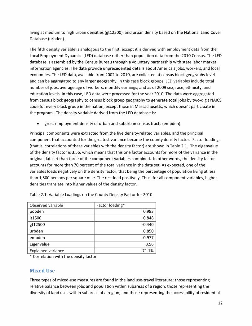
Principal components were extracted from the five density-related variables, and the principal
component that accounted for the greatest variance became the county density factor. Factor loadings
(that is, correlations of these variables with the density factor) are shown in Table 2.1. The eigenvalue
of the density factor is 3.56, which means that this one factor accounts for more of the variance in the
original dataset than three of the component variables combined. In other words, the density factor
accounts for more than 70 percent of the total variance in the data set. As expected, one of the
variables loads negatively on the density factor, that being the percentage of population living at less
than 1,500 persons per square mile. The rest load positively. Thus, for all component variables, higher
densities translate into higher values of the density factor.
Table 2.1. Variable Loadings on the County Density Factor for 2010
Observed variable Factor loading*
popden 0.983
lt1500 0.848
gt12500 -0.440
urbden 0.850
empden 0.977
Eigenvalue 3.56
Explained variance 71.1%
* Correlation with the density factor
Mixed Use
Three types of mixed-use measures are found in the land use-travel literature: those representing
relative balance between jobs and population within subareas of a region; those representing the
diversity of land uses within subareas of a region; and those representing the accessibility of residential
13
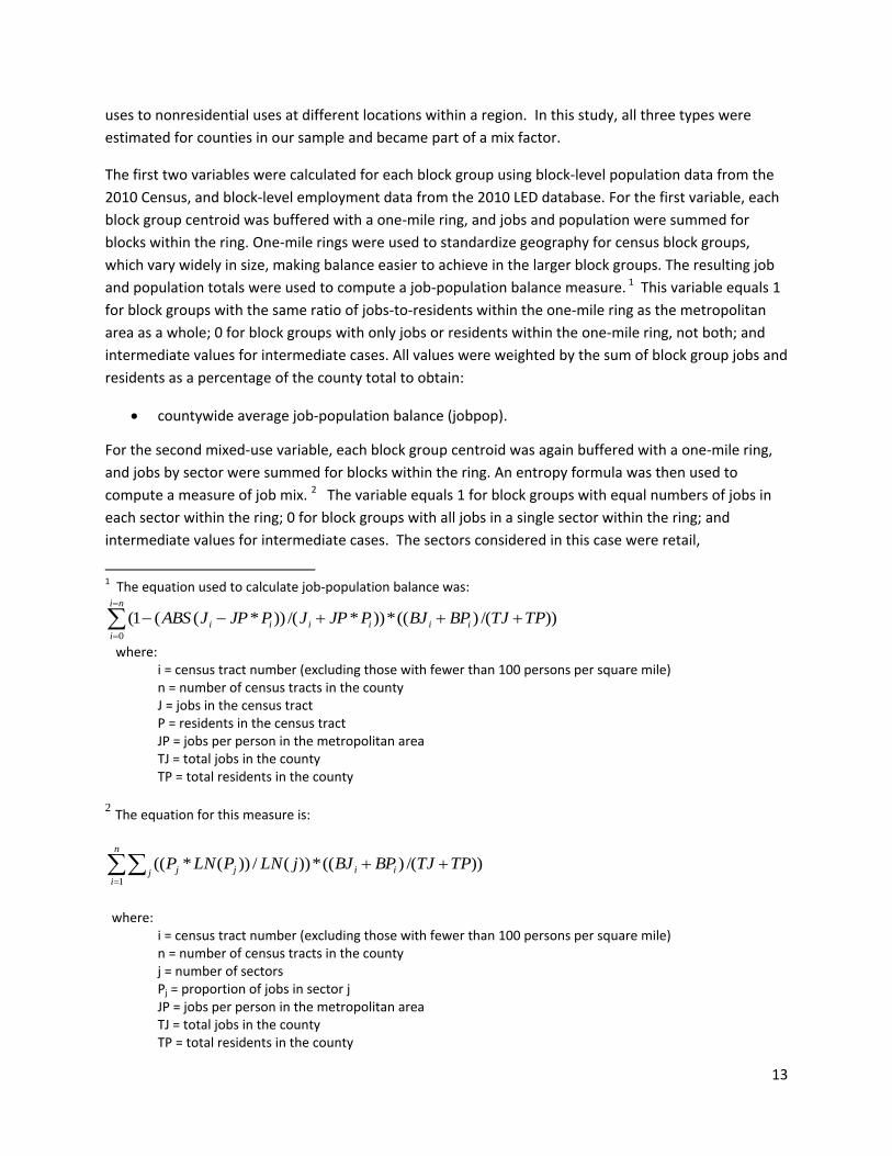
uses to nonresidential uses at different locations within a region. In this study, all three types were
estimated for counties in our sample and became part of a mix factor.
The first two variables were calculated for each block group using block-level population data from the
2010 Census, and block-level employment data from the 2010 LED database. For the first variable, each
block group centroid was buffered with a one-mile ring, and jobs and population were summed for
blocks within the ring. One-mile rings were used to standardize geography for census block groups,
which vary widely in size, making balance easier to achieve in the larger block groups. The resulting job
and population totals were used to compute a job-population balance measure. 1 This variable equals 1
for block groups with the same ratio of jobs-to-residents within the one-mile ring as the metropolitan
area as a whole; 0 for block groups with only jobs or residents within the one-mile ring, not both; and
intermediate values for intermediate cases. All values were weighted by the sum of block group jobs and
residents as a percentage of the county total to obtain:
countywide average job-population balance (jobpop).
For the second mixed-use variable, each block group centroid was again buffered with a one-mile ring,
and jobs by sector were summed for blocks within the ring. An entropy formula was then used to
compute a measure of job mix. 2 The variable equals 1 for block groups with equal numbers of jobs in
each sector within the ring; 0 for block groups with all jobs in a single sector within the ring; and
intermediate values for intermediate cases. The sectors considered in this case were retail,
1 The equation used to calculate job-population balance was:
ni
i
iiiiii TPTJBPBJPJPJPJPJABS0
))/()((*))*/())*((1(
where: i = census tract number (excluding those with fewer than 100 persons per square mile) n = number of census tracts in the county J = jobs in the census tract P = residents in the census tract JP = jobs per person in the metropolitan area TJ = total jobs in the county TP = total residents in the county
2 The equation for this measure is:
n
i
iij jj TPTJBPBJjLNPLNP1
))/()((*))(/))(*((
where: i = census tract number (excluding those with fewer than 100 persons per square mile) n = number of census tracts in the county j = number of sectors Pj = proportion of jobs in sector j JP = jobs per person in the metropolitan area TJ = total jobs in the county TP = total residents in the county
14
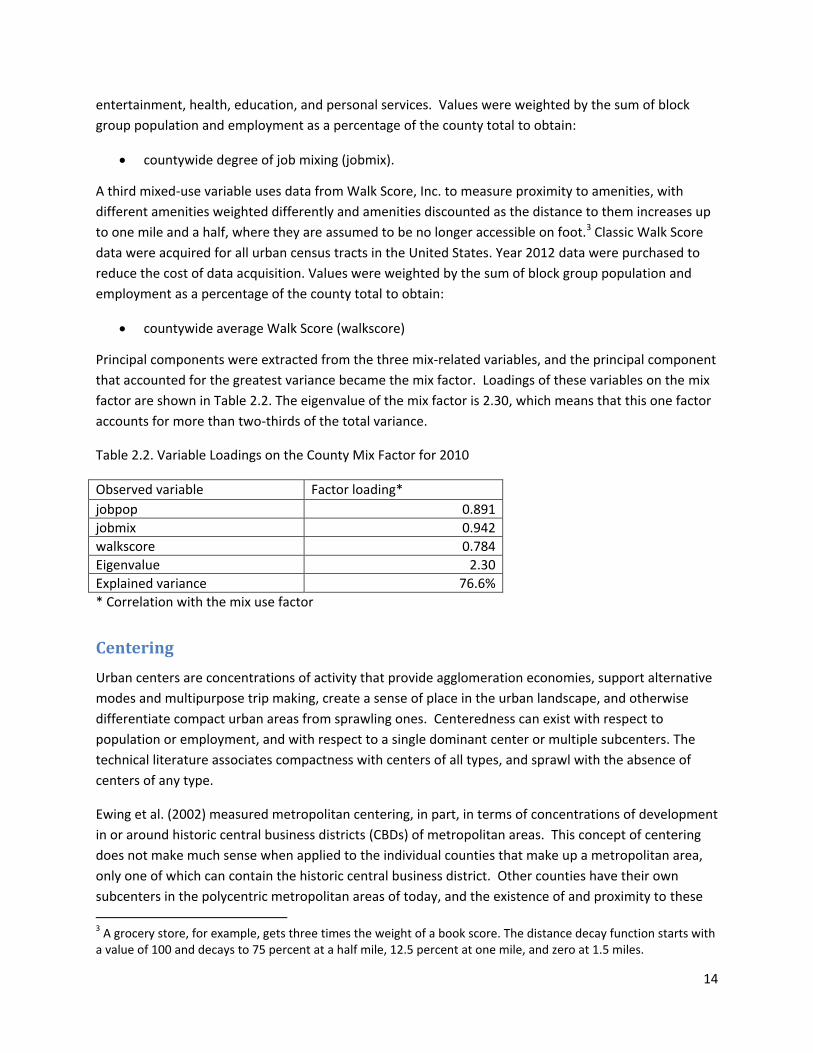
entertainment, health, education, and personal services. Values were weighted by the sum of block
group population and employment as a percentage of the county total to obtain:
countywide degree of job mixing (jobmix).
A third mixed-use variable uses data from Walk Score, Inc. to measure proximity to amenities, with
different amenities weighted differently and amenities discounted as the distance to them increases up
to one mile and a half, where they are assumed to be no longer accessible on foot.3 Classic Walk Score
data were acquired for all urban census tracts in the United States. Year 2012 data were purchased to
reduce the cost of data acquisition. Values were weighted by the sum of block group population and
employment as a percentage of the county total to obtain:
countywide average Walk Score (walkscore)
Principal components were extracted from the three mix-related variables, and the principal component
that accounted for the greatest variance became the mix factor. Loadings of these variables on the mix
factor are shown in Table 2.2. The eigenvalue of the mix factor is 2.30, which means that this one factor
accounts for more than two-thirds of the total variance.
Table 2.2. Variable Loadings on the County Mix Factor for 2010
Observed variable Factor loading*
jobpop 0.891
jobmix 0.942
walkscore 0.784
Eigenvalue 2.30
Explained variance 76.6%
* Correlation with the mix use factor
Centering
Urban centers are concentrations of activity that provide agglomeration economies, support alternative
modes and multipurpose trip making, create a sense of place in the urban landscape, and otherwise
differentiate compact urban areas from sprawling ones. Centeredness can exist with respect to
population or employment, and with respect to a single dominant center or multiple subcenters. The
technical literature associates compactness with centers of all types, and sprawl with the absence of
centers of any type.
Ewing et al. (2002) measured metropolitan centering, in part, in terms of concentrations of development
in or around historic central business districts (CBDs) of metropolitan areas. This concept of centering
does not make much sense when applied to the individual counties that make up a metropolitan area,
only one of which can contain the historic central business district. Other counties have their own
subcenters in the polycentric metropolitan areas of today, and the existence of and proximity to these
3 A grocery store, for example, gets three times the weight of a book score. The distance decay function starts with a value of 100 and decays to 75 percent at a half mile, 12.5 percent at one mile, and zero at 1.5 miles.
15
are what distinguish counties with concentrations of activity from those without. Four measures of
centering were derived for metropolitan counties:
The first centering measure came straight out of the 2010 census:
coefficient of variation in census block group population densities, defined as the standard
deviation of block group densities divided by the average density of block groups. The more
variation in densities around the mean, the more centering and/or subcentering exists within
the county (varpop)
The second centering measure was derived from the LED database and is analogous to the first
measure, except for its use of employment density by block group rather than population density to
compute:
coefficient of variation in census block group employment densities, defined as the standard
deviation of block group densities divided by the average density of block groups. The more
variation in densities around the mean, the more centering and/or subcentering exists within
the county (varemp)
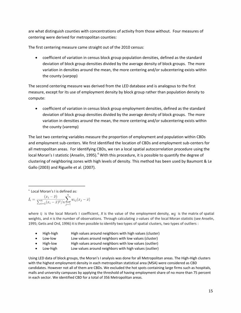
The last two centering variables measure the proportion of employment and population within CBDs
and employment sub-centers. We first identified the location of CBDs and employment sub-centers for
all metropolitan areas. For identifying CBDs, we ran a local spatial autocorrelation procedure using the
local Moran’s I statistic (Anselin, 1995).4 With this procedure, it is possible to quantify the degree of
clustering of neighboring zones with high levels of density. This method has been used by Baumont & Le
Gallo (2003) and Riguelle et al. (2007).
Local Moran’s I is defined as:
where Ii is the local Moran’s I coefficient, X is the value of the employment density, wij is the matrix of spatial
weights, and n is the number of observations. Through calculating z-values of the local Moran statistic (see Anselin,
1995; Getis and Ord, 1996) it is then possible to identify two types of spatial clusters, two types of outliers :
High-high High values around neighbors with high values (cluster)
Low-low Low values around neighbors with low values (cluster)
High-low High values around neighbors with low values (outlier)
Low-high Low values around neighbors with high values (outlier) Using LED data of block groups, the Moran’s I analysis was done for all Metropolitan areas. The High-High clusters with the highest employment density in each metropolitan statistical area (MSA) were considered as CBD candidates. However not all of them are CBDs. We excluded the hot spots containing large firms such as hospitals, malls and university campuses by applying the threshold of having employment share of no more than 75 percent in each sector. We identified CBD for a total of 356 Metropolitan areas.
16
Having CBDs for 356 metropolitan areas, we identified employment sub-centers as the positive residuals
estimated from an exponential employment density function using Geographically Weighted Regression
method (GWR).5 In the literature, urban sub-centers are areas with significantly higher employment
density than the surrounding areas (McDonald 1987). To identify sub-centers, researchers have used
several types of procedures: a minimum density procedure (Giuliano and Small 1991), identification of
local peaks (Craig & Ng, 2001), and a nonparametric method (McMillen 2004). The last of these methods
works best, according to literature review by Lee (2007). Using this procedure, we found 224
metropolitan areas to be monocentric (have only one center), 132 to be polycentric (have more than
one center), and 18 metropolitan areas to be dispersed (have no CBD and no sub-center). This
procedure resulted in two new centering variables. These findings were validated by inspecting Google
Earth satellite images to identify concentrations of activity, and see whether they corresponded to our
findings with GWR.
Percentage of county population in CBD or sub-centers (popcen)
Percentage of county employment in CBD or sub-centers (empcen)
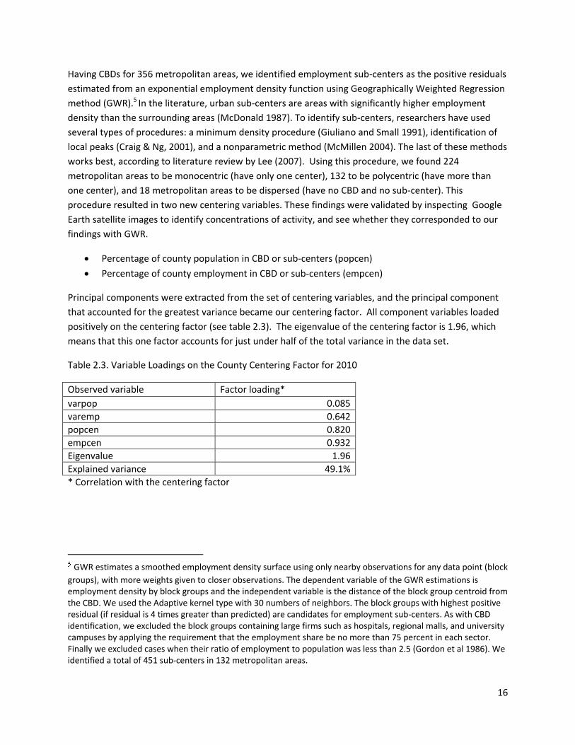
Principal components were extracted from the set of centering variables, and the principal component
that accounted for the greatest variance became our centering factor. All component variables loaded
positively on the centering factor (see table 2.3). The eigenvalue of the centering factor is 1.96, which
means that this one factor accounts for just under half of the total variance in the data set.
Table 2.3. Variable Loadings on the County Centering Factor for 2010
Observed variable Factor loading*
varpop 0.085
varemp 0.642
popcen 0.820
empcen 0.932
Eigenvalue 1.96
Explained variance 49.1%
* Correlation with the centering factor
GWR estimates a smoothed employment density surface using only nearby observations for any data point (block
groups), with more weights given to closer observations. The dependent variable of the GWR estimations is employment density by block groups and the independent variable is the distance of the block group centroid from the CBD. We used the Adaptive kernel type with 30 numbers of neighbors. The block groups with highest positive residual (if residual is 4 times greater than predicted) are candidates for employment sub-centers. As with CBD identification, we excluded the block groups containing large firms such as hospitals, regional malls, and university campuses by applying the requirement that the employment share be no more than 75 percent in each sector. Finally we excluded cases when their ratio of employment to population was less than 2.5 (Gordon et al 1986). We identified a total of 451 sub-centers in 132 metropolitan areas.
17
Street Accessibility
In the refined sprawl indices, two street variables are the same as in the original county sprawl index: average block size excluding rural blocks of more than one square mile (avgblk) and percentage of small urban blocks of less than one hundredth of a square mile (smlblk). To these two street accessibility variables were added. The two new street variables are:
intersection density for urban and suburban census tracts within the county, excluding ruraltracts with gross densities of less than 100 persons per square mile (intden)
percentage of 4-or-more-way intersections, again excluding rural tracts (4-way)
Intersection density captures both block length and street connectivity. Percentage of 4-or-more-way intersections provides a pure measure of street connectivity, as 4-way intersections provide more routing options than 3-way intersections.
Starting with a 2006 national dataset of street centerlines generated by TomTom that ships with ArcGIS, we produced a national database of street intersection locations, including for each intersection feature a count of streets that meet there. The TomTom dataset includes one centerline feature for each road segment running between neighboring intersections; i.e. every intersection is the spatially coincident endpoint of 3 or more road segments.6
The resulting national intersection database contains 13.1 million features; 77% of these are three-way intersections, and the remaining 23% are four- or more-way intersections. Total counts of 3- and 4-or-more-way intersections were tabulated for census tracts, and census tracts were aggregated to obtain county-level data. For each county, the total number of intersections in urban and suburban tracts was divided by the land area to obtain intersection density (intden), while the number of 4-or-more-way intersections was multiplied by 100 and divided by the total number of intersections to obtain the percentage of 4-or-more way intersections (4way).
6 Intersection features were created as follows: Using Census Feature Class Code (CFCC) values, we filtered out all freeways, unpaved tracks, and other roadways that don't function as pedestrian routes. Divided roadways, which from a pedestrian mobility perspective function similarly to undivided roadways of the same functional class, were represented in the source data as pairs of (roughly) parallel centerline segments. These were identified by CFCC value and merged into single segments using GIS tools. Streets intersecting the original divided roadways were trimmed or extended to the new merged centerlines, and the new merged centerlines were split at each intersection with side streets such that centerline features only intersect each other at feature endpoints. Roundabouts were assumed to function similarly to single 4+-way intersections, rather than close-set clusters of intersections joining the roundabout proper and the incoming streets. As such, centroids of roundabout circles were located and assigned an assumed count of four incoming streets; endpoints of incoming street features were ignored.
With the corrected street centerline data prepared, we generated point features at both endpoints of each street segment. Points closer together than 12m were adjusted to be spatially coincident in order to control for any possible remaining geometric errors related to divided roadways. We then used GIS tools to count the number of points (representing ends of street segments) coinciding at any location. Locations with point counts of one (dead ends) or two (locations where a roadway changes name, functional class, or other attribute) were discarded as non-street intersections. Remaining locations were flagged with attributes indicating whether a point was a three-way or a four- or more-way intersection.
18
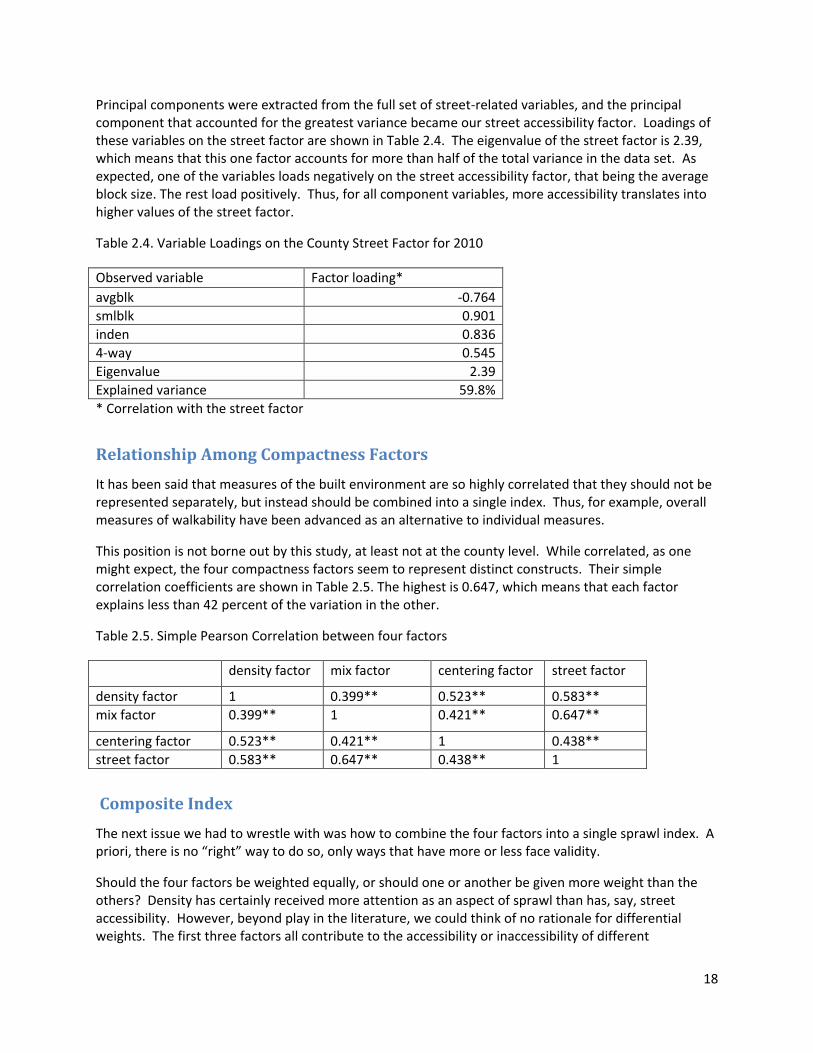
Principal components were extracted from the full set of street-related variables, and the principal component that accounted for the greatest variance became our street accessibility factor. Loadings of these variables on the street factor are shown in Table 2.4. The eigenvalue of the street factor is 2.39, which means that this one factor accounts for more than half of the total variance in the data set. As expected, one of the variables loads negatively on the street accessibility factor, that being the average block size. The rest load positively. Thus, for all component variables, more accessibility translates into higher values of the street factor.
Table 2.4. Variable Loadings on the County Street Factor for 2010
Observed variable Factor loading*
avgblk -0.764
smlblk 0.901
inden 0.836
4-way 0.545
Eigenvalue 2.39
Explained variance 59.8%
* Correlation with the street factor
Relationship Among Compactness Factors
It has been said that measures of the built environment are so highly correlated that they should not be represented separately, but instead should be combined into a single index. Thus, for example, overall measures of walkability have been advanced as an alternative to individual measures.
This position is not borne out by this study, at least not at the county level. While correlated, as one might expect, the four compactness factors seem to represent distinct constructs. Their simple correlation coefficients are shown in Table 2.5. The highest is 0.647, which means that each factor explains less than 42 percent of the variation in the other.
Table 2.5. Simple Pearson Correlation between four factors
density factor mix factor centering factor street factor
density factor 1 0.399** 0.523** 0.583**
mix factor 0.399** 1 0.421** 0.647**
centering factor 0.523** 0.421** 1 0.438**
street factor 0.583** 0.647** 0.438** 1
Composite Index
The next issue we had to wrestle with was how to combine the four factors into a single sprawl index. A priori, there is no “right” way to do so, only ways that have more or less face validity.
Should the four factors be weighted equally, or should one or another be given more weight than the others? Density has certainly received more attention as an aspect of sprawl than has, say, street accessibility. However, beyond play in the literature, we could think of no rationale for differential weights. The first three factors all contribute to the accessibility or inaccessibility of different
19
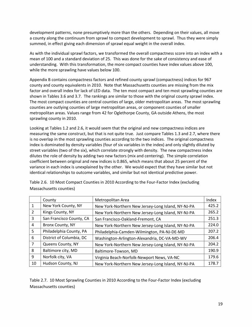
development patterns, none presumptively more than the others. Depending on their values, all move a county along the continuum from sprawl to compact development to sprawl. Thus they were simply summed, in effect giving each dimension of sprawl equal weight in the overall index.
As with the individual sprawl factors, we transformed the overall compactness score into an index with a mean of 100 and a standard deviation of 25. This was done for the sake of consistency and ease of understanding. With this transformation, the more compact counties have index values above 100, while the more sprawling have values below 100.
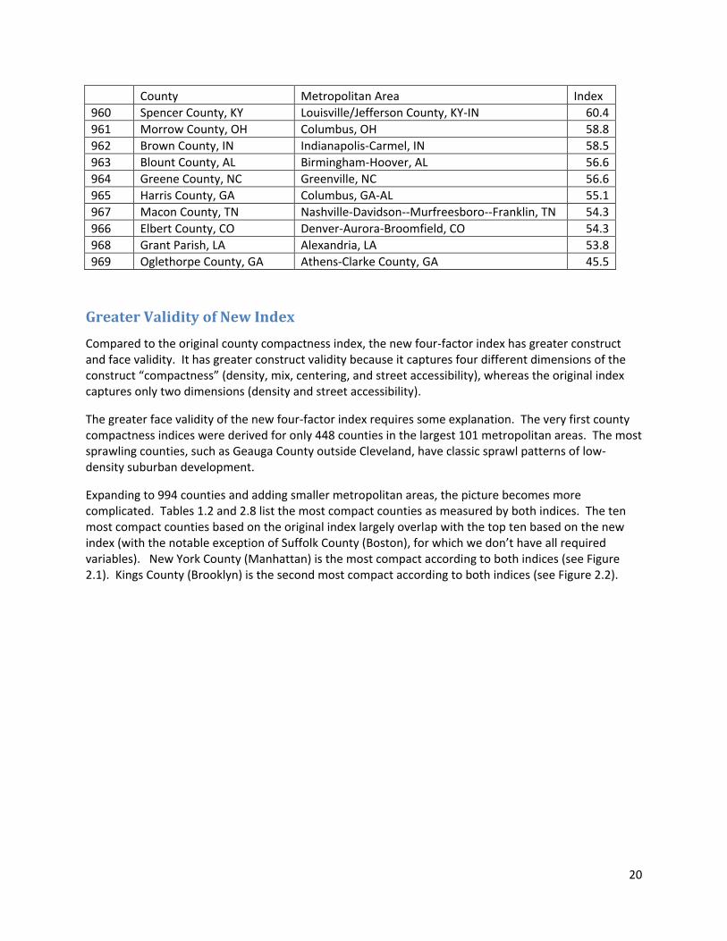
Appendix B contains compactness factors and refined county sprawl (compactness) indices for 967 county and county equivalents in 2010. Note that Massachusetts counties are missing from the mix factor and overall index for lack of LED data. The ten most compact and ten most sprawling counties are shown in Tables 3.6 and 3.7. The rankings are similar to those with the original county sprawl index. The most compact counties are central counties of large, older metropolitan areas. The most sprawling counties are outlying counties of large metropolitan areas, or component counties of smaller metropolitan areas. Values range from 42 for Oglethorpe County, GA outside Athens, the most sprawling county in 2010.
Looking at Tables 1.2 and 2.6, it would seem that the original and new compactness indices are measuring the same construct, but that is not quite true. Just compare Tables 1.3 and 2.7, where there is no overlap in the most sprawling counties according to the two indices. The original compactness index is dominated by density variables (four of six variables in the index) and only slightly diluted by street variables (two of the six), which correlate strongly with density. The new compactness index dilutes the role of density by adding two new factors (mix and centering). The simple correlation coefficient between original and new indices is 0.865, which means that about 25 percent of the variance in each index is unexplained by the other. We would expect that they have similar but not identical relationships to outcome variables, and similar but not identical predictive power.
Table 2.6. 10 Most Compact Counties in 2010 According to the Four-Factor Index (excluding
Massachusetts counties)
County Metropolitan Area Index
1 New York County, NY New York-Northern New Jersey-Long Island, NY-NJ-PA 425.2
2 Kings County, NY New York-Northern New Jersey-Long Island, NY-NJ-PA 265.2
3 San Francisco County, CA San Francisco-Oakland-Fremont, CA 251.3
4 Bronx County, NY New York-Northern New Jersey-Long Island, NY-NJ-PA 224.0
5 Philadelphia County, PA Philadelphia-Camden-Wilmington, PA-NJ-DE-MD 207.2
6 District of Columbia, DC Washington-Arlington-Alexandria, DC-VA-MD-WV 206.4
7 Queens County, NY New York-Northern New Jersey-Long Island, NY-NJ-PA 204.2
8 Baltimore city, MD Baltimore-Towson, MD 190.9
9 Norfolk city, VA Virginia Beach-Norfolk-Newport News, VA-NC 179.6
10 Hudson County, NJ New York-Northern New Jersey-Long Island, NY-NJ-PA 178.7
Table 2.7. 10 Most Sprawling Counties in 2010 According to the Four-Factor Index (excluding
Massachusetts counties)
20
County Metropolitan Area Index
960 Spencer County, KY Louisville/Jefferson County, KY-IN 60.4
961 Morrow County, OH Columbus, OH 58.8
962 Brown County, IN Indianapolis-Carmel, IN 58.5
963 Blount County, AL Birmingham-Hoover, AL 56.6
964 Greene County, NC Greenville, NC 56.6
965 Harris County, GA Columbus, GA-AL 55.1
967 Macon County, TN Nashville-Davidson--Murfreesboro--Franklin, TN 54.3
966 Elbert County, CO Denver-Aurora-Broomfield, CO 54.3
968 Grant Parish, LA Alexandria, LA 53.8
969 Oglethorpe County, GA Athens-Clarke County, GA 45.5
Greater Validity of New Index
Compared to the original county compactness index, the new four-factor index has greater construct and face validity. It has greater construct validity because it captures four different dimensions of the construct “compactness” (density, mix, centering, and street accessibility), whereas the original index captures only two dimensions (density and street accessibility).
The greater face validity of the new four-factor index requires some explanation. The very first county compactness indices were derived for only 448 counties in the largest 101 metropolitan areas. The most sprawling counties, such as Geauga County outside Cleveland, have classic sprawl patterns of low-density suburban development.
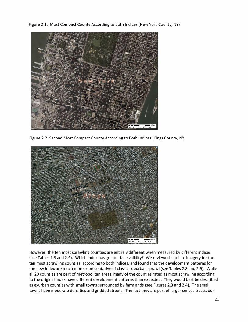
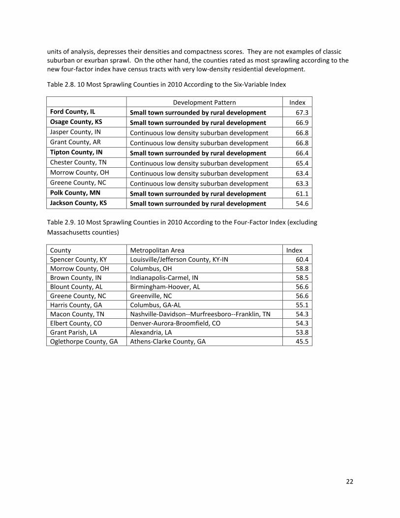
Expanding to 994 counties and adding smaller metropolitan areas, the picture becomes more complicated. Tables 1.2 and 2.8 list the most compact counties as measured by both indices. The ten most compact counties based on the original index largely overlap with the top ten based on the new index (with the notable exception of Suffolk County (Boston), for which we don’t have all required variables). New York County (Manhattan) is the most compact according to both indices (see Figure 2.1). Kings County (Brooklyn) is the second most compact according to both indices (see Figure 2.2).
21
Figure 2.1. Most Compact County According to Both Indices (New York County, NY)
Figure 2.2. Second Most Compact County According to Both Indices (Kings County, NY)
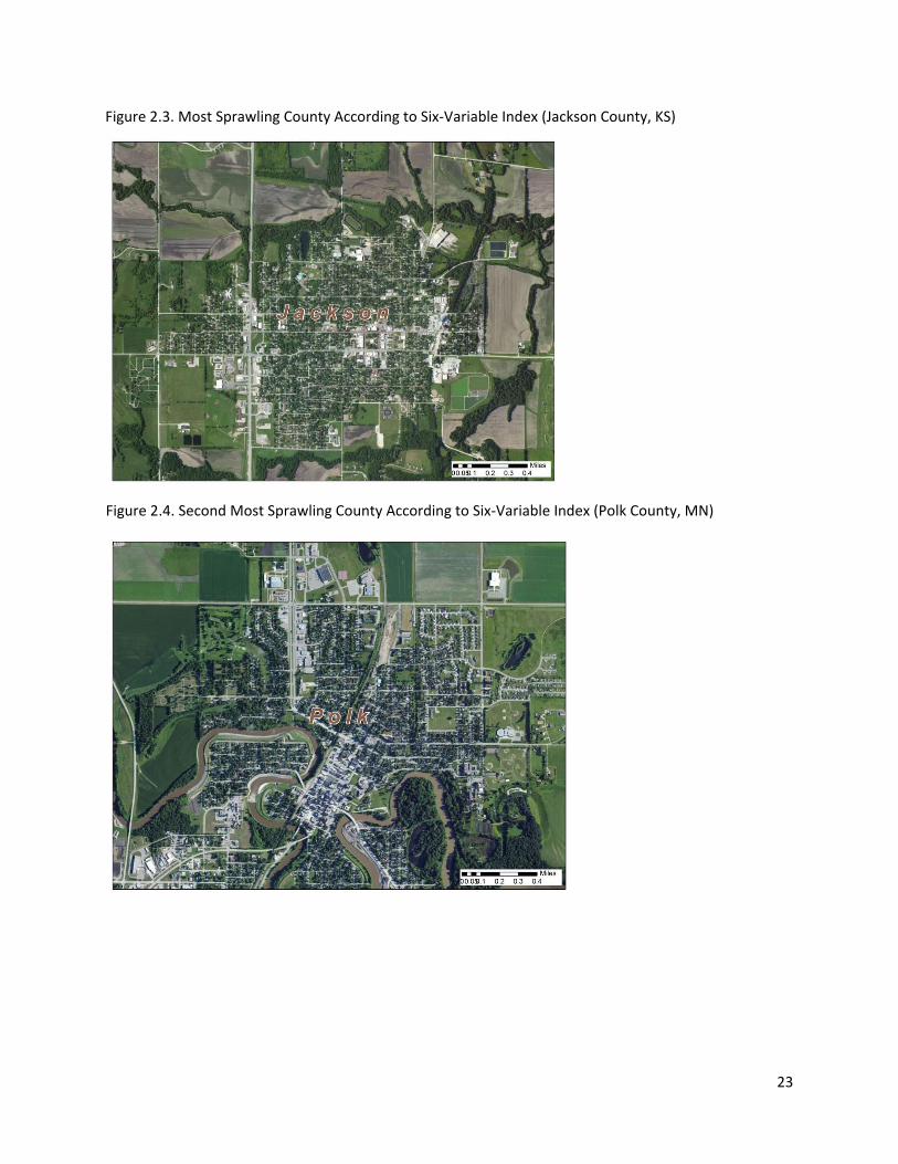
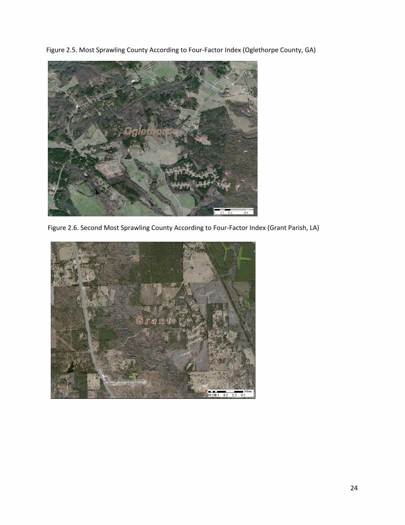
However, the ten most sprawling counties are entirely different when measured by different indices (see Tables 1.3 and 2.9). Which index has greater face validity? We reviewed satellite imagery for the ten most sprawling counties, according to both indices, and found that the development patterns for the new index are much more representative of classic suburban sprawl (see Tables 2.8 and 2.9). While all 20 counties are part of metropolitan areas, many of the counties rated as most sprawling according to the original index have different development patterns than expected. They would best be described as exurban counties with small towns surrounded by farmlands (see Figures 2.3 and 2.4). The small towns have moderate densities and gridded streets. The fact they are part of larger census tracts, our
22
units of analysis, depresses their densities and compactness scores. They are not examples of classic suburban or exurban sprawl. On the other hand, the counties rated as most sprawling according to the new four-factor index have census tracts with very low-density residential development.
Table 2.8. 10 Most Sprawling Counties in 2010 According to the Six-Variable Index
Development Pattern Index
Ford County, IL Small town surrounded by rural development 67.3
Osage County, KS Small town surrounded by rural development 66.9
Jasper County, IN Continuous low density suburban development 66.8
Grant County, AR Continuous low density suburban development 66.8
Tipton County, IN Small town surrounded by rural development 66.4
Chester County, TN Continuous low density suburban development 65.4
Morrow County, OH Continuous low density suburban development 63.4
Greene County, NC Continuous low density suburban development 63.3
Polk County, MN Small town surrounded by rural development 61.1
Jackson County, KS Small town surrounded by rural development 54.6
Table 2.9. 10 Most Sprawling Counties in 2010 According to the Four-Factor Index (excluding
Massachusetts counties)
County Metropolitan Area Index
Spencer County, KY Louisville/Jefferson County, KY-IN 60.4
Morrow County, OH Columbus, OH 58.8
Brown County, IN Indianapolis-Carmel, IN 58.5
Blount County, AL Birmingham-Hoover, AL 56.6
Greene County, NC Greenville, NC 56.6
Harris County, GA Columbus, GA-AL 55.1
Macon County, TN Nashville-Davidson--Murfreesboro--Franklin, TN 54.3
Elbert County, CO Denver-Aurora-Broomfield, CO 54.3
Grant Parish, LA Alexandria, LA 53.8
Oglethorpe County, GA Athens-Clarke County, GA 45.5
23
Figure 2.3. Most Sprawling County According to Six-Variable Index (Jackson County, KS)
Figure 2.4. Second Most Sprawling County According to Six-Variable Index (Polk County, MN)
24
Figure 2.5. Most Sprawling County According to Four-Factor Index (Oglethorpe County, GA)
Figure 2.6. Second Most Sprawling County According to Four-Factor Index (Grant Parish, LA)
25
Chapter 3. Derivation of Metropolitan Sprawl Indices
Sprawl is ordinarily conceptualized at the metropolitan level, encompassing cities and their suburbs. When we say Atlanta sprawls badly, we are probably referring to metropolitan Atlanta, not the city of Atlanta or Fulton County. The focus up to this point in the report has been on counties, because counties are typically smaller than metropolitan areas and more homogeneous than metropolitan areas. They more closely correspond to the environment in which individuals live, work, and play on a daily basis, and hence are affected by the built environment. But certain phenomena are manifested at the regional or metropolitan level, such as ozone levels and racial segregation. So in this chapter we derive metropolitan sprawl indices.
Methods
Sample
The unit of analysis in this study is the metropolitan area. A metropolitan area is a region that consists of a densely populated urban core and its less-populated surrounding territories that are economically and socially linked to it. The criteria of defining metropolitan areas changed in 2003. Smaller MSAs remained the same, but larger metropolitan areas, previously referred to as consolidated metropolitan statistical areas (CMSAs) are now defined as MSAs. Different portions of CMSAs, previously referred to as primary metropolitan statistical areas (PMSAs), have been redefined and reconfigured as metropolitan divisions. For example, the old New York CMSA consisted of eleven counties in two states and four PMSAs: New York PMSA, Nassau-Suffolk PMSA, Dutchess County PMSA and Newburgh, NY-PA PMSA. The current New York MSA consists of twenty-three counties in three states and four metropolitan divisions. The New York MSA now is strikingly heterogeneous, whereas the old New York PMSA contained only the five boroughs that make up New York City. Metropolitan divisions do not perfectly substitute for PMSAs, as they have different size thresholds (2.5 million vs. 1 million population), but they come as close to representing homogenous units as we can come with current census geography. Metropolitan divisions are designated for each of the eleven largest MSAs.7 The sample in this study is limited to medium and large metropolitan areas, and metropolitan divisions where they are defined. It initially included a total of 228 areas with more than 200,000 population in 2010. The rationale for thus limiting our sample is simple: the concept of sprawl has particular relevance to large areas where the economic, social, and environmental consequences of sprawl can be significant. The concept of sprawl does not have much relevance to small MSAs such as Lewiston, ID and Casper, WY. Parenthetically, a total of seven metropolitan areas and divisions were ultimately dropped from our sample due to the lack of local employment dynamics (LED) data, a key data source for measuring sprawl. These metropolitan areas, or a portion of them, are located in Massachusetts, which does not participate in the LED program. This reduces the final sample size to 221 MSAs and metropolitan divisions.
7 The metropolitan divisions, as components of MSAs, somewhat resemble PMSAs under the old system. However, PMSAs were much more common. The higher population threshold for establishing metropolitan divisions (at least 2.5 million), opposed to the threshold of at least 1 million to establish PMSAs, means that the new system contains twenty-nine metropolitan divisions within eleven MSAs, compared to seventy-three PMSAs within eighteen CMSAs under the old system.
26
Variables
Development Density
Our first five density variables are the same as in the original sprawl index (Ewing et al., 2002): gross density of urban and suburban census tracts (popden), percentage of the population living at low suburban densities (lt1500), percentage of the population living at medium to high urban densities (gt12500), and urban density based on the National Land Cover Database (urbden). These variables are measured the same way for metropolitan areas as for counties (see Chapter 2). A fifth variable is the estimated density at the center of the metropolitan area derived from a negative exponential density function (dgcent). The function assumes the form: Di = Do exp (-b di). where: Di = the density of census tract i Do = the estimated density at the center of the metropolitan area b = the estimated density gradient or rate of decline of density with distance di = the distance of the census tract from the center of the principal city The higher the central density, and the steeper the density function, the more compact the metropolitan area (in a monocentric sense).8 The sixth density variable, which is new, is analogous to the first, except it is derived with employment data from the Local Employment Dynamics (LED) database (empden). The LED data were aggregated from census block geography to generate total jobs by 2-digit NAICS code for every block group in the nation. This was then divided by land area to produce a density measure. The last two variables are related to employment centers identified by the authors as a part of this study. For more information on how the centers were identified for MSAs see “Activity Centering” in Chapter 3.The two variables are weighted average population density (popdcen) and weighted average employment density (empdcen) of all centers within a metropolitan area. The average densities were weighted by the sum of block group jobs and residents as a percentage of the MSA total.
Land Use Mix
The two mixed-use variables were calculated for each block group’s buffer using block-level population data from the 2010 Census, and block-level employment data from the 2010 LED database. The first variable is a job-population balance measure (jobpop). This variable equals 1 for block groups with the same ratio of jobs-to-residents within the one-mile ring as the metropolitan area as a whole; 0 for block groups with only jobs or residents within the one-mile ring, not both; and intermediate values for
8 The function was estimated as follows. The principal cities of the metro areas were identified as the first-named cities in the 1990 definitions of those areas. Their centers were determined by locating central business district tracts within the principal cities as specified in the 1980 STF3 file. 1980 designations were adopted because central business districts have not been designated since then. The means of the latitudes and longitudes of the centroids of those central business district tracts were taken as the metropolitan centers. The distances from the centers to all tracts were calculated using an ArcGIS. Finally, a negative exponential density function was fit to the resulting data points to estimate the intercept and density gradient.
27
intermediate cases. All values were weighted by the sum of block group jobs and residents as a percentage of the MSA total. 9 We also derived a job mix variable (jobmix). The variable, an entropy measure, equals 1 for block groups with equal numbers of jobs in each sector; 0 for block groups with all jobs in a single sector within the ring; and intermediate values for intermediate cases. The sectors considered in this case were retail, entertainment, health, education, and personal services. Values were weighted by the sum of block group population and employment as a percentage of the MSA total. A third mixed-use variable is metropolitan weighted average Walk Score (walkscore). It was computed using data from Walk Score, Inc. to measure proximity to amenities, with different amenities weighted differently and amenities discounted as the distance to them increases up to one mile and a half, where they are assumed to be no longer accessible on foot.10 Classic Walk Score data were acquired for all urban census tracts in the United States. Values were weighted by the sum of census tract population and employment as a percentage of the MSA total.
Activity Centering
The first centering variable came straight out of Ewing et al. (2002) and the 2010 census. It is the coefficient of variation in census block group population densities, defined as the standard deviation of block group densities divided by the average density of block groups (varpop). The more variation in population densities around the mean, the more centering and/or subcentering exists within the MSA. The second centering variable is analogous to the first, except it is derived with employment data from the LED database. It is the coefficient of variation in census block group employment densities, defined as the standard deviation of block group densities divided by the average density of block groups (varemp). The more variation in employment densities around the mean, the more centering and/or subcentering exists within the MSAs. The third variable contributing to the centering factor is the density gradient moving outward from the CBD, estimated with a negative exponential density function. The faster density declines with distance from the center, the more centered (in a monocentric sense) the metropolitan area will be (dgrad). The next two centering variables measure the proportion of employment and population within CBDs and employment sub-centers. For computing them, we first identified the location of CBDs and employment sub-centers for all metropolitan areas (see “Activity Centering” section on Chapter 3). This procedure resulted in two new centering variables as the percentage of MSA population (popcen) and employment (empcen) in CBDs and sub-centers.
Street Accessibility
Street accessibility is related to block size since smaller blocks translate into shorter and more direct routes. Large block sizes indicate a lack of street connections and alternate routes. So, three street accessibility variables were computed for each MSA based on blocks size: average block length (avgblklngh), average block size (avgblksze) and the percentage of blocks that are less than 1/100 square mile, which is the typical size of an urban block (smlblk).
9 See “land use mix” section for the formula used for computing job-population balance and job mix measures. 10 A grocery store, for example, gets three times the weight of a book score. The distance decay function starts with
a value of 100 and decays to 75 percent at a half mile, 12.5 percent at one mile, and zero at 1.5 miles.
28
These three variables were part of Ewing et al.’s original sprawl metrics. To them, we have added two new variables. They are intersection density and percentage of 4-or-more way intersections. Intersections are where street connections are made and cars must stop to allow pedestrians to cross. The higher the intersection density, the more walkable the city (Jacobs, 1993). Intersection density has become the most common metric in studies of built environmental impacts on individual travel behavior (Ewing and Cervero, 2010). Another common metric in such studies is the percentage of 4-or-more-way intersections (Ewing and Cervero, 2010). This metric provides the purest measure of street connectivity, as 4-way intersections provide more routing options than 3-way intersections. A high percentage of 4-way intersections does not guarantee walkability, as streets may connect at 4-way intersections in a super grid of arterials. But it does guarantee routing options. For each MSA, the total number of intersections in the urbanized portion of MSA was divided by the land area to obtain intersection density (intden), while the number of 4-or-more-way intersections was multiplied by 100 and divided by the total number of intersections to obtain the percentage of 4-or-more way intersections (4way).
Results
Individual Compactness/Sprawl Factors
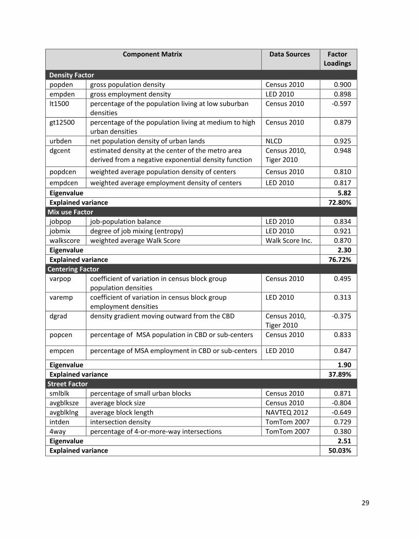
For each dimension of sprawl, we ran principal component analysis on the measured variables, and the principal component that captured the largest share of common variance among the measured variables was selected to represent that dimension. Factor loadings (the correlation between a variable and a principal component), eigenvalues (the explanatory power of a single principal component), and percentages of explained variance are shown in Table 3.1. The eigenvalue of the density factor is 5.82, which indicates that this one factor accounts for about three quarters of the total variance in the dataset. As anticipated, the percentage of the population living at less than 1,500 persons per square mile loads negatively on the density factor. The rest load positively. The eigenvalue for the mix factor is 2.30, which indicates that this one factor accounts for more than three quarter of the total variance in the dataset. All component variables load positively on the mix factor. The eigenvalue of the centering factor is 1.90, which indicates that this factor accounts for about 38% of the total variance in the datasets. The density gradient loads negatively on centering factor as expected. The rest load positively. The eigenvalue of the street factor is 2.51, which indicates that this factor accounts for more than a half of the total variance in the dataset. As expected, the average block size and average block length load negatively on the street accessibility factor. The rest load positively.
Table 3.1: Variable Loadings of Four Factors for 2010
29
Component Matrix Data Sources Factor Loadings
Density Factor
popden gross population density Census 2010 0.900
empden gross employment density LED 2010 0.898
lt1500
percentage of the population living at low suburban densities
Census 2010 -0.597
gt12500
percentage of the population living at medium to high urban densities
Census 2010 0.879
urbden net population density of urban lands NLCD 0.925
dgcent estimated density at the center of the metro area derived from a negative exponential density function
Census 2010, Tiger 2010
0.948
popdcen weighted average population density of centers Census 2010 0.810
empdcen weighted average employment density of centers LED 2010 0.817
Eigenvalue 5.82
Explained variance 72.80%
Mix use Factor
jobpop job-population balance LED 2010 0.834
jobmix degree of job mixing (entropy) LED 2010 0.921
walkscore weighted average Walk Score Walk Score Inc. 0.870
Eigenvalue 2.30
Explained variance 76.72%
Centering Factor
varpop coefficient of variation in census block group population densities
Census 2010 0.495
varemp coefficient of variation in census block group employment densities
LED 2010 0.313
dgrad density gradient moving outward from the CBD Census 2010, Tiger 2010
-0.375
popcen percentage of MSA population in CBD or sub-centers Census 2010 0.833
empcen percentage of MSA employment in CBD or sub-centers LED 2010 0.847
Eigenvalue 1.90
Explained variance 37.89%
Street Factor
smlblk percentage of small urban blocks Census 2010 0.871
avgblksze average block size Census 2010 -0.804
avgblklng average block length NAVTEQ 2012 -0.649
intden intersection density TomTom 2007 0.729
4way percentage of 4-or-more-way intersections TomTom 2007 0.380
Eigenvalue 2.51
Explained variance 50.03%
30
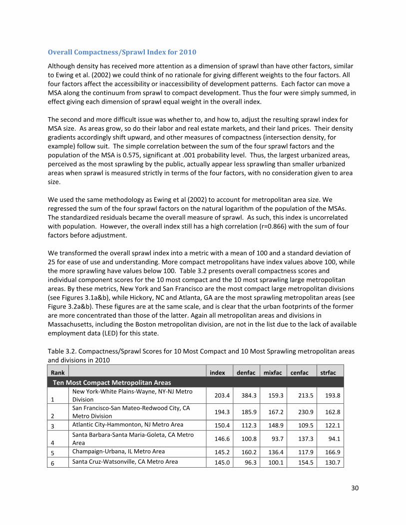
Overall Compactness/Sprawl Index for 2010
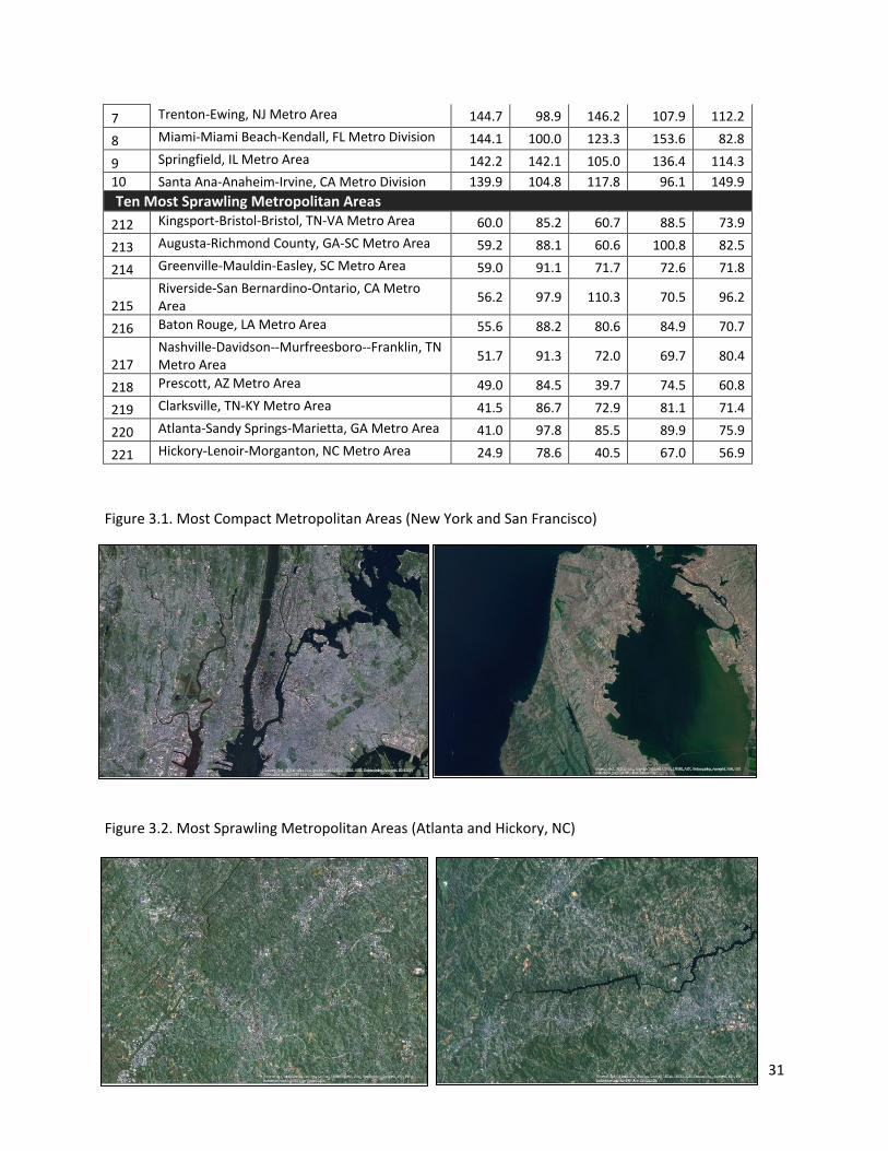
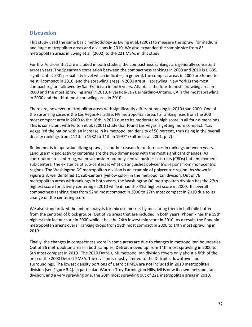
Although density has received more attention as a dimension of sprawl than have other factors, similar to Ewing et al. (2002) we could think of no rationale for giving different weights to the four factors. All four factors affect the accessibility or inaccessibility of development patterns. Each factor can move a MSA along the continuum from sprawl to compact development. Thus the four were simply summed, in effect giving each dimension of sprawl equal weight in the overall index. The second and more difficult issue was whether to, and how to, adjust the resulting sprawl index for MSA size. As areas grow, so do their labor and real estate markets, and their land prices. Their density gradients accordingly shift upward, and other measures of compactness (intersection density, for example) follow suit. The simple correlation between the sum of the four sprawl factors and the population of the MSA is 0.575, significant at .001 probability level. Thus, the largest urbanized areas, perceived as the most sprawling by the public, actually appear less sprawling than smaller urbanized areas when sprawl is measured strictly in terms of the four factors, with no consideration given to area size. We used the same methodology as Ewing et al (2002) to account for metropolitan area size. We regressed the sum of the four sprawl factors on the natural logarithm of the population of the MSAs. The standardized residuals became the overall measure of sprawl. As such, this index is uncorrelated with population. However, the overall index still has a high correlation (r=0.866) with the sum of four factors before adjustment. We transformed the overall sprawl index into a metric with a mean of 100 and a standard deviation of 25 for ease of use and understanding. More compact metropolitans have index values above 100, while the more sprawling have values below 100. Table 3.2 presents overall compactness scores and individual component scores for the 10 most compact and the 10 most sprawling large metropolitan areas. By these metrics, New York and San Francisco are the most compact large metropolitan divisions (see Figures 3.1a&b), while Hickory, NC and Atlanta, GA are the most sprawling metropolitan areas (see Figure 3.2a&b). These figures are at the same scale, and is clear that the urban footprints of the former are more concentrated than those of the latter. Again all metropolitan areas and divisions in Massachusetts, including the Boston metropolitan division, are not in the list due to the lack of available employment data (LED) for this state.
Table 3.2. Compactness/Sprawl Scores for 10 Most Compact and 10 Most Sprawling metropolitan areas and divisions in 2010
Rank index denfac mixfac cenfac strfac
Ten Most Compact Metropolitan Areas
1 New York-White Plains-Wayne, NY-NJ Metro Division
203.4 384.3 159.3 213.5 193.8
2 San Francisco-San Mateo-Redwood City, CA Metro Division
194.3 185.9 167.2 230.9 162.8
3 Atlantic City-Hammonton, NJ Metro Area 150.4 112.3 148.9 109.5 122.1
4 Santa Barbara-Santa Maria-Goleta, CA Metro Area
146.6 100.8 93.7 137.3 94.1
5 Champaign-Urbana, IL Metro Area 145.2 160.2 136.4 117.9 166.9
6 Santa Cruz-Watsonville, CA Metro Area 145.0 96.3 100.1 154.5 130.7
31
7 Trenton-Ewing, NJ Metro Area 144.7 98.9 146.2 107.9 112.2
8 Miami-Miami Beach-Kendall, FL Metro Division 144.1 100.0 123.3 153.6 82.8
9 Springfield, IL Metro Area 142.2 142.1 105.0 136.4 114.3
10 Santa Ana-Anaheim-Irvine, CA Metro Division 139.9 104.8 117.8 96.1 149.9
Ten Most Sprawling Metropolitan Areas
212 Kingsport-Bristol-Bristol, TN-VA Metro Area 60.0 85.2 60.7 88.5 73.9
213 Augusta-Richmond County, GA-SC Metro Area 59.2 88.1 60.6 100.8 82.5
214 Greenville-Mauldin-Easley, SC Metro Area 59.0 91.1 71.7 72.6 71.8
215 Riverside-San Bernardino-Ontario, CA Metro Area
56.2 97.9 110.3 70.5 96.2
216 Baton Rouge, LA Metro Area 55.6 88.2 80.6 84.9 70.7
217 Nashville-Davidson--Murfreesboro--Franklin, TN Metro Area
51.7 91.3 72.0 69.7 80.4
218 Prescott, AZ Metro Area 49.0 84.5 39.7 74.5 60.8
219 Clarksville, TN-KY Metro Area 41.5 86.7 72.9 81.1 71.4
220 Atlanta-Sandy Springs-Marietta, GA Metro Area 41.0 97.8 85.5 89.9 75.9
221 Hickory-Lenoir-Morganton, NC Metro Area 24.9 78.6 40.5 67.0 56.9
Figure 3.1. Most Compact Metropolitan Areas (New York and San Francisco)
Figure 3.2. Most Sprawling Metropolitan Areas (Atlanta and Hickory, NC)
32
Discussion
This study used the same basic methodology as Ewing et al. (2002) to measure the sprawl for medium and large metropolitan areas and divisions in 2010. We also expanded the sample size from 83 metropolitan areas in Ewing et al. (2002) to the 221 MSAs in this study. For the 76 areas that are included in both studies, the compactness rankings are generally consistent across years. The Spearman correlation between the compactness rankings in 2000 and 2010 is 0.635, significant at .001 probability level which indicates, in general, the compact areas in 2000 are found to be still compact in 2010; and the sprawling areas in 2000 are still sprawling. New York is the most compact region followed by San Francisco in both years. Atlanta is the fourth most sprawling area in 2000 and the most sprawling area in 2010. Riverside-San Bernardino-Ontario, CA is the most sprawling in 2000 and the third most sprawling area in 2010. There are, however, metropolitan areas with significantly different ranking in 2010 than 2000. One of the surprising cases is the Las Vegas-Paradise, NV metropolitan area. Its ranking rises from the 30th most compact area in 2000 to the 16th in 2010 due to its moderate to high score in all four dimensions. This is consistent with Fulton et al. (2001) study that found Las Vegas is getting more compact. “Las Vegas led the nation with an increase in its metropolitan density of 50 percent, thus rising in the overall density rankings from 114th in 1982 to 14th in 1997” (Fulton et al. 2001, p: 7). Refinements in operationalizing sprawl, is another reason for differences in rankings between years. Land use mix and activity centering are the two dimensions with the most significant changes. As contributors to centering, we now consider not only central business districts (CBDs) but employment sub-centers. The existence of sub-centers is what distinguishes polycentric regions from monocentric regions. The Washington DC metropolitan division is an example of polycentric region. As shown in Figure 3.3, we identified 11 sub-centers (yellow color) in the metropolitan division. Out of 76 metropolitan areas with rankings in both years, the Washington DC metropolitan division has the 27th highest score for activity centering in 2010 while it had the 41st highest score in 2000. Its overall compactness ranking rises from 52nd most compact in 2000 to 27th most compact in 2010 due to its change on the centering score. We also standardized the unit of analysis for mix use metrics by measuring them in half mile buffers from the centroid of block groups. Out of 76 areas that are included in both years, Phoenix has the 19th highest mix factor score in 2000 while it has the 24th lowest mix score in 2010. As a result, the Phoenix metropolitan area’s overall ranking drops from 18th most compact in 2000 to 14th most sprawling in 2010. Finally, the changes in compactness score in some areas are due to changes in metropolitan boundaries. Out of 76 metropolitan areas in both samples, Detroit moved up from 14th most sprawling in 2000 to 5th most compact in 2010. The 2010 Detroit, MI metropolitan division covers only about a fifth of the area of the 2000 Detroit PMSA. The division is mostly limited to the Detroit’s downtown and surroundings. The lowest density portions of Detroit PMSA are not included in 2010 metropolitan division (see Figure 3.4). In particular, Warren-Troy-Farmington Hills, MI is now its own metropolitan division, and a very sprawling one, the 20th most sprawling out of 221 metropolitan areas in 2010.
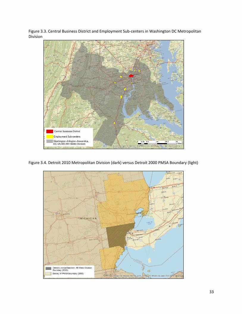
33
Figure 3.3. Central Business District and Employment Sub-centers in Washington DC Metropolitan Division
Figure 3.4. Detroit 2010 Metropolitan Division (dark) versus Detroit 2000 PMSA Boundary (light)
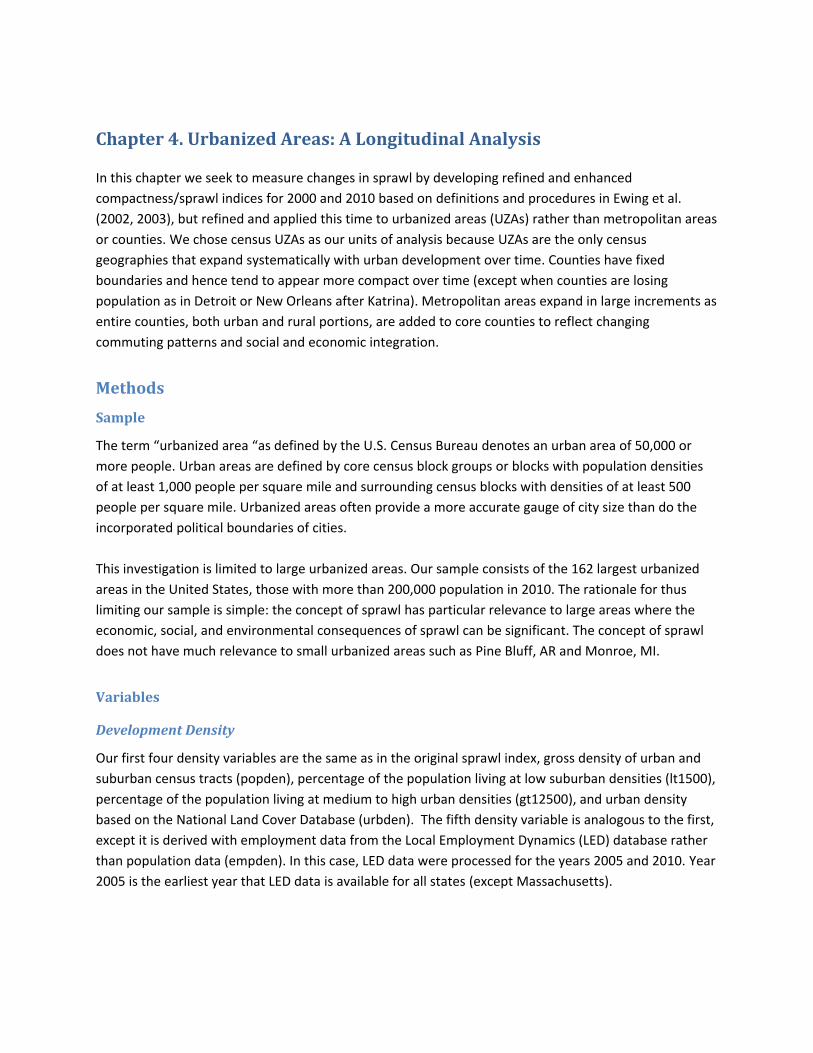
Chapter 4. Urbanized Areas: A Longitudinal Analysis
In this chapter we seek to measure changes in sprawl by developing refined and enhanced
compactness/sprawl indices for 2000 and 2010 based on definitions and procedures in Ewing et al.
(2002, 2003), but refined and applied this time to urbanized areas (UZAs) rather than metropolitan areas
or counties. We chose census UZAs as our units of analysis because UZAs are the only census
geographies that expand systematically with urban development over time. Counties have fixed
boundaries and hence tend to appear more compact over time (except when counties are losing
population as in Detroit or New Orleans after Katrina). Metropolitan areas expand in large increments as
entire counties, both urban and rural portions, are added to core counties to reflect changing
commuting patterns and social and economic integration.
Methods
Sample
The term “urbanized area “as defined by the U.S. Census Bureau denotes an urban area of 50,000 or
more people. Urban areas are defined by core census block groups or blocks with population densities
of at least 1,000 people per square mile and surrounding census blocks with densities of at least 500
people per square mile. Urbanized areas often provide a more accurate gauge of city size than do the
incorporated political boundaries of cities.
This investigation is limited to large urbanized areas. Our sample consists of the 162 largest urbanized
areas in the United States, those with more than 200,000 population in 2010. The rationale for thus
limiting our sample is simple: the concept of sprawl has particular relevance to large areas where the
economic, social, and environmental consequences of sprawl can be significant. The concept of sprawl
does not have much relevance to small urbanized areas such as Pine Bluff, AR and Monroe, MI.
Variables
Development Density
Our first four density variables are the same as in the original sprawl index, gross density of urban and
suburban census tracts (popden), percentage of the population living at low suburban densities (lt1500),
percentage of the population living at medium to high urban densities (gt12500), and urban density
based on the National Land Cover Database (urbden). The fifth density variable is analogous to the first,
except it is derived with employment data from the Local Employment Dynamics (LED) database rather
than population data (empden). In this case, LED data were processed for the years 2005 and 2010. Year
2005 is the earliest year that LED data is available for all states (except Massachusetts).
MEASURING URBAN SPRAWL AND VALIDATING SPRAWL MEASURES
80
Land Use Mix
Although using the same variables as Ewing et al. (2002) to operationalize mixed use, we computed
them differently using one-mile buffers around the centers of block groups rather than computing them
within the boundaries of block groups.
The two mixed use variables were calculated for each block group’s buffer using block-level population
data from the 2010 Census, and block-level employment data from the 2010 LED database. The resulting
job and population totals were used to compute a job-population balance measure (jobpop). This
variable equals 1 for block groups with the same ratio of jobs-to-residents within the one-mile ring as
the urbanized area as a whole; 0 for block groups with only jobs or residents within the one-mile ring,
not both; and intermediate values for intermediate cases. All values were weighted by the sum of block
group jobs and residents as a percentage of the UZA total.
For the second mixed-use variable, each block group centroid was again buffered with a one-mile ring,
and jobs by sector were summed for blocks within the ring. An entropy formula was then used to
compute a measure of job mix (jobmix). The variable equals 1 for block groups with equal numbers of
jobs in each sector within the ring; 0 for block groups with all jobs in a single sector within the ring; and
intermediate values for intermediate cases. The sectors considered in this case were retail,
entertainment, health, education, and personal services. Values were weighted by the sum of block
group population and employment as a percentage of the urbanized areas total. 11
Unlike the mixed use factors at the county and metropolitan levels, the mixed use factor at the
urbanized area level does not include a third variables, Walk Score. The reason is simple. This is
longitudinal comparison of sprawl in 2000 and 2010, and Walk Score data were not available until 2007.
Activity Centering
The first centering variable came straight out of Ewing et al. (2002, 2003) and the 2010 census. It is the
coefficient of variation in census block group population densities, defined as the standard deviation of
block group densities divided by the average density of block groups (varpop). The more variation in
population densities around the mean, the more centering and/or subcentering exists within the
urbanized areas.
The second centering variable is analogous to the first, except it is derived with employment data from
the LED database. It is the coefficient of variation in census block group employment densities, defined
as the standard deviation of block group densities divided by the average density of block groups
(varemp). The more variation in employment densities around the mean, the more centering and/or
subcentering exists within the urbanized areas.
11 See “land use mix” section for the formula used for computing job-population balance and job mix measures.
MEASURING URBAN SPRAWL AND VALIDATING SPRAWL MEASURES
81
The next two centering variables measure the proportion of employment and population within CBDs
and employment sub-centers. We first identified the location of CBDs and employment sub-centers for
all metropolitan areas (see Chapter 3). This procedure resulted in two new centering variables as the
percentage of UZA population (popcen) and employment (empcen) in CBDs and sub-centers.
Street Accessibility
Street accessibility is related to block size since smaller blocks translate into shorter and more direct
routes. Large block sizes indicate a relative paucity of street connections and alternate routes. So, two
street accessibility variables were computed for each urbanized area: average block size (avgblk) and
percentage of blocks with areas less than 1/100 square mile, the size of a typical traditional urban block
bounded by sides just over 500 feet in length (smlblk).
These two variables were part of Ewing et al.’s original sprawl metrics. To them, we have added two
new variables. They are intersection density and percentage of 4-or-more way intersections.
For each UZA, the total number of intersections in the UZA was divided by the land area to obtain
intersection density (intden), while the number of 4-or-more-way intersections was multiplied by 100
and divided by the total number of intersections to obtain the percentage of 4-or-more way
intersections (4way).
Statistical Methods
In this study we use two statistical methods. Principal component analysis (a type of factor analysis) is
used to derive individual compactness indices that represent the built environments of UZAs. Then
linear regression analysis is used to relate these indices to transportation outcomes, controlling for
influences other than the built environment.
For each dimension of sprawl, principal components were extracted from the component variables. The
principal component selected to represent the dimension was the one capturing the largest share of
common variance among the component variables, that is, the one upon which the observed variables
loaded most heavily. Because, in this study, the first component captured the majority of the combined
variance of these variables, no subsequent components were considered.
The other statistical method used in this study is linear regression (ordinary least squares or OLS). Our
dependent variables were logged so as to be normally distributed and hence properly modeled with
regression analysis. As for the independent variables (control variables), we transformed all variables
into log form to achieve a better fit with the data, reduce the influence of outliers, and adjust for
nonlinearity of the data. The transformations have the added advantage of allowing us to interpret
regression coefficients as elasticities. An elasticity is a percentage change in one variable that
accompanies a one percent change in another variable. Elasticities are the most common measures of
effect size in both economics and planning.
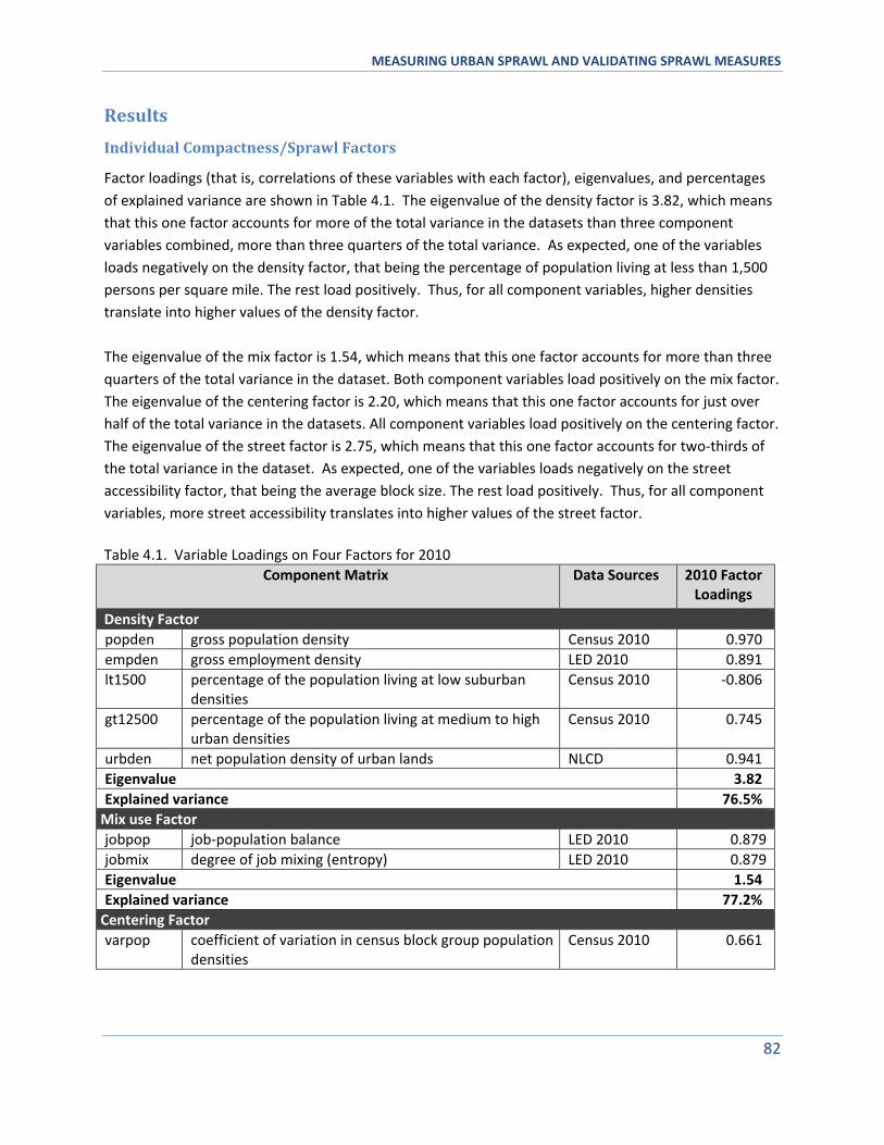
MEASURING URBAN SPRAWL AND VALIDATING SPRAWL MEASURES
82
Results
Individual Compactness/Sprawl Factors
Factor loadings (that is, correlations of these variables with each factor), eigenvalues, and percentages
of explained variance are shown in Table 4.1. The eigenvalue of the density factor is 3.82, which means
that this one factor accounts for more of the total variance in the datasets than three component
variables combined, more than three quarters of the total variance. As expected, one of the variables
loads negatively on the density factor, that being the percentage of population living at less than 1,500
persons per square mile. The rest load positively. Thus, for all component variables, higher densities
translate into higher values of the density factor.
The eigenvalue of the mix factor is 1.54, which means that this one factor accounts for more than three
quarters of the total variance in the dataset. Both component variables load positively on the mix factor.
The eigenvalue of the centering factor is 2.20, which means that this one factor accounts for just over
half of the total variance in the datasets. All component variables load positively on the centering factor.
The eigenvalue of the street factor is 2.75, which means that this one factor accounts for two-thirds of
the total variance in the dataset. As expected, one of the variables loads negatively on the street
accessibility factor, that being the average block size. The rest load positively. Thus, for all component
variables, more street accessibility translates into higher values of the street factor.
Table 4.1. Variable Loadings on Four Factors for 2010
Component Matrix Data Sources 2010 Factor Loadings
Density Factor
popden gross population density Census 2010 0.970
empden gross employment density LED 2010 0.891
lt1500
percentage of the population living at low suburban densities
Census 2010 -0.806
gt12500
percentage of the population living at medium to high urban densities
Census 2010 0.745
urbden net population density of urban lands NLCD 0.941
Eigenvalue 3.82
Explained variance 76.5%
Mix use Factor
jobpop job-population balance LED 2010 0.879
jobmix degree of job mixing (entropy) LED 2010 0.879
Eigenvalue 1.54
Explained variance 77.2%
Centering Factor
varpop coefficient of variation in census block group population densities
Census 2010 0.661
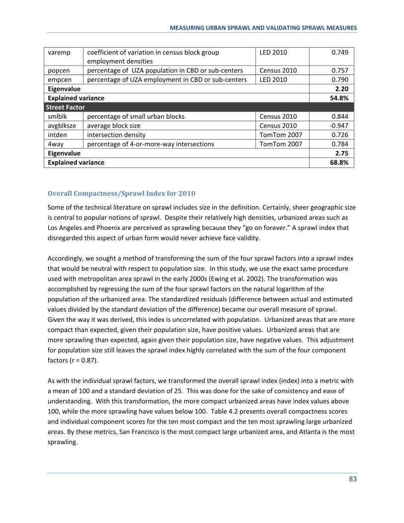
MEASURING URBAN SPRAWL AND VALIDATING SPRAWL MEASURES
83
varemp coefficient of variation in census block group employment densities
LED 2010 0.749
popcen percentage of UZA population in CBD or sub-centers Census 2010 0.757
empcen percentage of UZA employment in CBD or sub-centers LED 2010 0.790
Eigenvalue 2.20
Explained variance 54.8%
Street Factor
smlblk percentage of small urban blocks Census 2010 0.844
avgblksze average block size Census 2010 -0.947
intden intersection density TomTom 2007 0.726
4way percentage of 4-or-more-way intersections TomTom 2007 0.784
Eigenvalue 2.75
Explained variance 68.8%
Overall Compactness/Sprawl Index for 2010
Some of the technical literature on sprawl includes size in the definition. Certainly, sheer geographic size
is central to popular notions of sprawl. Despite their relatively high densities, urbanized areas such as
Los Angeles and Phoenix are perceived as sprawling because they “go on forever.” A sprawl index that
disregarded this aspect of urban form would never achieve face validity.
Accordingly, we sought a method of transforming the sum of the four sprawl factors into a sprawl index
that would be neutral with respect to population size. In this study, we use the exact same procedure
used with metropolitan area sprawl in the early 2000s (Ewing et al. 2002). The transformation was
accomplished by regressing the sum of the four sprawl factors on the natural logarithm of the
population of the urbanized area. The standardized residuals (difference between actual and estimated
values divided by the standard deviation of the difference) became our overall measure of sprawl.
Given the way it was derived, this index is uncorrelated with population. Urbanized areas that are more
compact than expected, given their population size, have positive values. Urbanized areas that are
more sprawling than expected, again given their population size, have negative values. This adjustment
for population size still leaves the sprawl index highly correlated with the sum of the four component
factors (r = 0.87).
As with the individual sprawl factors, we transformed the overall sprawl index (index) into a metric with
a mean of 100 and a standard deviation of 25. This was done for the sake of consistency and ease of
understanding. With this transformation, the more compact urbanized areas have index values above
100, while the more sprawling have values below 100. Table 4.2 presents overall compactness scores
and individual component scores for the ten most compact and the ten most sprawling large urbanized
areas. By these metrics, San Francisco is the most compact large urbanized area, and Atlanta is the most
sprawling.
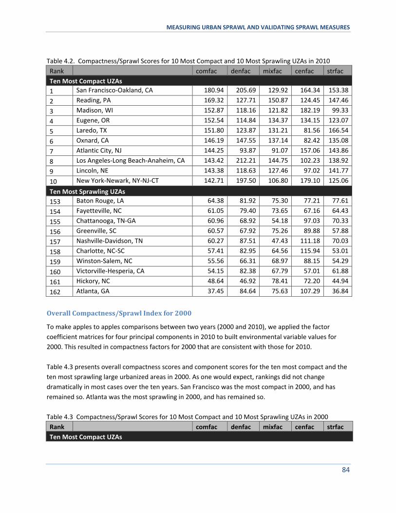
MEASURING URBAN SPRAWL AND VALIDATING SPRAWL MEASURES
84
Table 4.2. Compactness/Sprawl Scores for 10 Most Compact and 10 Most Sprawling UZAs in 2010
Rank comfac denfac mixfac cenfac strfac
Ten Most Compact UZAs
1 San Francisco-Oakland, CA 180.94 205.69 129.92 164.34 153.38
2 Reading, PA 169.32 127.71 150.87 124.45 147.46
3 Madison, WI 152.87 118.16 121.82 182.19 99.33
4 Eugene, OR 152.54 114.84 134.37 134.15 123.07
5 Laredo, TX 151.80 123.87 131.21 81.56 166.54
6 Oxnard, CA 146.19 147.55 137.14 82.42 135.08
7 Atlantic City, NJ 144.25 93.87 91.07 157.06 143.86
8 Los Angeles-Long Beach-Anaheim, CA 143.42 212.21 144.75 102.23 138.92
9 Lincoln, NE 143.38 118.63 127.46 97.02 141.77
10 New York-Newark, NY-NJ-CT 142.71 197.50 106.80 179.10 125.06
Ten Most Sprawling UZAs
153 Baton Rouge, LA 64.38 81.92 75.30 77.21 77.61
154 Fayetteville, NC 61.05 79.40 73.65 67.16 64.43
155 Chattanooga, TN-GA 60.96 68.92 54.18 97.03 70.33
156 Greenville, SC 60.57 67.92 75.26 89.88 57.88
157 Nashville-Davidson, TN 60.27 87.51 47.43 111.18 70.03
158 Charlotte, NC-SC 57.41 82.95 64.56 115.94 53.01
159 Winston-Salem, NC 55.56 66.31 68.97 88.15 54.29
160 Victorville-Hesperia, CA 54.15 82.38 67.79 57.01 61.88
161 Hickory, NC 48.64 46.92 78.41 72.20 44.94
162 Atlanta, GA 37.45 84.64 75.63 107.29 36.84
Overall Compactness/Sprawl Index for 2000
To make apples to apples comparisons between two years (2000 and 2010), we applied the factor
coefficient matrices for four principal components in 2010 to built environmental variable values for
2000. This resulted in compactness factors for 2000 that are consistent with those for 2010.
Table 4.3 presents overall compactness scores and component scores for the ten most compact and the
ten most sprawling large urbanized areas in 2000. As one would expect, rankings did not change
dramatically in most cases over the ten years. San Francisco was the most compact in 2000, and has
remained so. Atlanta was the most sprawling in 2000, and has remained so.
Table 4.3 Compactness/Sprawl Scores for 10 Most Compact and 10 Most Sprawling UZAs in 2000
Rank comfac denfac mixfac cenfac strfac
Ten Most Compact UZAs
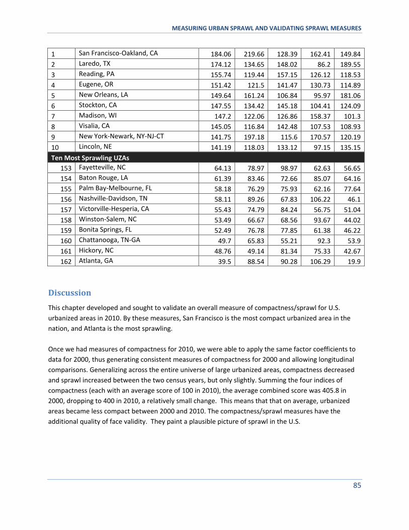
MEASURING URBAN SPRAWL AND VALIDATING SPRAWL MEASURES
85
1 San Francisco-Oakland, CA 184.06 219.66 128.39 162.41 149.84
2 Laredo, TX 174.12 134.65 148.02 86.2 189.55
3 Reading, PA 155.74 119.44 157.15 126.12 118.53
4 Eugene, OR 151.42 121.5 141.47 130.73 114.89
5 New Orleans, LA 149.64 161.24 106.84 95.97 181.06
6 Stockton, CA 147.55 134.42 145.18 104.41 124.09
7 Madison, WI 147.2 122.06 126.86 158.37 101.3
8 Visalia, CA 145.05 116.84 142.48 107.53 108.93
9 New York-Newark, NY-NJ-CT 141.75 197.18 115.6 170.57 120.19
10 Lincoln, NE 141.19 118.03 133.12 97.15 135.15
Ten Most Sprawling UZAs
153 Fayetteville, NC 64.13 78.97 98.97 62.63 56.65
154 Baton Rouge, LA 61.39 83.46 72.66 85.07 64.16
155 Palm Bay-Melbourne, FL 58.18 76.29 75.93 62.16 77.64
156 Nashville-Davidson, TN 58.11 89.26 67.83 106.22 46.1
157 Victorville-Hesperia, CA 55.43 74.79 84.24 56.75 51.04
158 Winston-Salem, NC 53.49 66.67 68.56 93.67 44.02
159 Bonita Springs, FL 52.49 76.78 77.85 61.38 46.22
160 Chattanooga, TN-GA 49.7 65.83 55.21 92.3 53.9
161 Hickory, NC 48.76 49.14 81.34 75.33 42.67
162 Atlanta, GA 39.5 88.54 90.28 106.29 19.9
Discussion
This chapter developed and sought to validate an overall measure of compactness/sprawl for U.S.
urbanized areas in 2010. By these measures, San Francisco is the most compact urbanized area in the
nation, and Atlanta is the most sprawling.
Once we had measures of compactness for 2010, we were able to apply the same factor coefficients to
data for 2000, thus generating consistent measures of compactness for 2000 and allowing longitudinal
comparisons. Generalizing across the entire universe of large urbanized areas, compactness decreased
and sprawl increased between the two census years, but only slightly. Summing the four indices of
compactness (each with an average score of 100 in 2010), the average combined score was 405.8 in
2000, dropping to 400 in 2010, a relatively small change. This means that that on average, urbanized
areas became less compact between 2000 and 2010. The compactness/sprawl measures have the
additional quality of face validity. They paint a plausible picture of sprawl in the U.S.
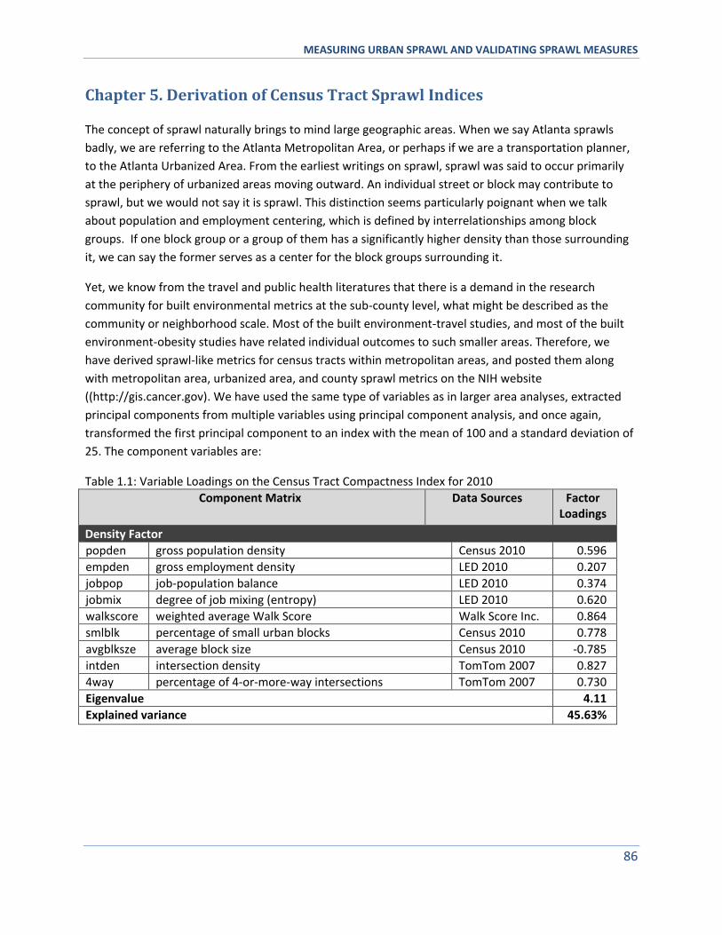
MEASURING URBAN SPRAWL AND VALIDATING SPRAWL MEASURES
86
Chapter 5. Derivation of Census Tract Sprawl Indices
The concept of sprawl naturally brings to mind large geographic areas. When we say Atlanta sprawls
badly, we are referring to the Atlanta Metropolitan Area, or perhaps if we are a transportation planner,
to the Atlanta Urbanized Area. From the earliest writings on sprawl, sprawl was said to occur primarily
at the periphery of urbanized areas moving outward. An individual street or block may contribute to
sprawl, but we would not say it is sprawl. This distinction seems particularly poignant when we talk
about population and employment centering, which is defined by interrelationships among block
groups. If one block group or a group of them has a significantly higher density than those surrounding
it, we can say the former serves as a center for the block groups surrounding it.
Yet, we know from the travel and public health literatures that there is a demand in the research
community for built environmental metrics at the sub-county level, what might be described as the
community or neighborhood scale. Most of the built environment-travel studies, and most of the built
environment-obesity studies have related individual outcomes to such smaller areas. Therefore, we
have derived sprawl-like metrics for census tracts within metropolitan areas, and posted them along
with metropolitan area, urbanized area, and county sprawl metrics on the NIH website
((http://gis.cancer.gov). We have used the same type of variables as in larger area analyses, extracted
principal components from multiple variables using principal component analysis, and once again,
transformed the first principal component to an index with the mean of 100 and a standard deviation of
25. The component variables are:
Table 1.1: Variable Loadings on the Census Tract Compactness Index for 2010
Component Matrix Data Sources Factor Loadings
Density Factor
popden gross population density Census 2010 0.596
empden gross employment density LED 2010 0.207
jobpop job-population balance LED 2010 0.374
jobmix degree of job mixing (entropy) LED 2010 0.620
walkscore weighted average Walk Score Walk Score Inc. 0.864
smlblk percentage of small urban blocks Census 2010 0.778
avgblksze average block size Census 2010 -0.785
intden intersection density TomTom 2007 0.827
4way percentage of 4-or-more-way intersections TomTom 2007 0.730
Eigenvalue 4.11
Explained variance 45.63%
MEASURING URBAN SPRAWL AND VALIDATING SPRAWL MEASURES
87
Chapter 6. Conclusion
This study has updated a county and metropolitan compactness/sprawl indices, widely used by planning and public researchers since their release in 2002 and 2003. The updated indices reflect conditions on the ground circa 2010.
This study has also developed new measures of compactness/sprawl that incorporate additional dimensions of the construct “sprawl,” and used additional variables to operationalize these dimensions. The four dimensions, measured individually and with a composite index, are development density, land use mix, activity centering, and street accessibility. Measures, presented in the Appendices, are immediately available to study the costs and benefits of different urban forms.
Using updated and enhanced measures of compactness/sprawl, this study has validated both the original and new indices, and largely validated the individual measures representing the four dimensions of sprawl. These new results mirror and confirm the earlier findings of Ewing et al. (2002, 2003a, 2003b, 2003c). If anything, relationships of sprawl to important quality-of-life outcomes are stronger than in the original studies.
An obvious question is whether the new measures have more face, construct, and internal validity than the original compactness/sprawl indices, and thus should substitute for the original indices in future research. They have more face validity because places that fit the definition of sprawl in satellite imagery rank lowest on compactness. They have more construct validity because they capture more aspect of sprawl. As for internal validity, they generally outperform the original county sprawl indices as predictors of negative outcomes.
The new multi-dimensional factors representing density, mix, centering, and streets are somewhat correlated, of course, but still quite distinct in their relationships to outcomes. We can see these being used to determine which specific aspects of sprawl result in costs and benefits.
MEASURING URBAN SPRAWL AND VALIDATING SPRAWL MEASURES
88
References
Anselin, L. (1995). Local indicators of spatial association—LISA. Geographical analysis, 27(2), 93-115.
Baumont, C., Ertur, C., Le Gallo, J. (2003). 4 Spatial Convergence Clubs and the European Regional
Growth Process, 1980. European regional growth, 131.
Bereitschaft, B., and K. Debbage. 2013. Urban Form, Air Pollution, and CO2 Emissions in Large U.S.
Metropolitan Areas. The Professional Geographer, 65(4), 612–635.
Cho, S., Z. Chen, S.T. Yen, and D.B. Eastwood. 2006. The Effects of Urban Sprawl on Body Mass Index:
Where People Live Does Matter. The 52nd Annual ACCI Conference, Baltimore, Maryland, March 15–18.
Craig, S. G., and P. T. Ng. 2001. Using quantile smoothing splines to identify employment subcenters in a
multicentric urban area. Journal of Urban Economics 49: 100-120.
Doyle, S., A. Kelly-Schwartz, M. Schlossberg, and J. Stockard. 2006. Active Community Environments and
Health: The Relationship of Walkable and Safe Communities to Individual Health. Journal of the
American Planning Association. 72(1), 19–31.
Ewing, R. (1997). Is Los Angeles-style sprawl desirable? Journal of the American Planning Association,
63(1), 107-126.
Ewing, R. and Cervero, R. (2001). Travel and the built environment. Transportation Research Record,
1780, 87-114.
Ewing R, Pendall R, Chen D. 2002. Measuring Sprawl and Its Impacts. Washington, DC: Smart Growth
America.
Ewing, R., R. Pendall, and D. Chen. 2003a. Measuring Sprawl and Its Transportation Impacts.
Transportation Research Record. 1832: 175-183.
Ewing R.,T. Schmid, R. Killingsworth, A. Zlot, and S. Raudenbush. 2003b. Relationship Between Urban
Sprawl and Physical Activity, Obesity, and Morbidity. American Journal of Health Promotion.18:47-57.
Ewing, R., R. Schieber and C. Zegeer. 2003c. Urban Sprawl as a Risk Factor in Motor Vehicle Occupant
and Pedestrian Fatalities, American Journal of Public Health 93: 1541-1545.
Ewing R., R. Brownson, and D. Berrigan. 2006. Relationship Between Urban Sprawl and Weight of U.S.
Youth. American Journal of Preventive Medicine. 31: 464-474.
Ewing, R. and F. Rong. 2008. Impact of Urban Form on U.S. Residential Energy Use. Housing Policy
Debate. 19: 1-30.
MEASURING URBAN SPRAWL AND VALIDATING SPRAWL MEASURES
89
Ewing, R., Cervero, R.: Travel and the built environment: a meta-analysis. Journal of the American
Planning Association 76(3), 265–294 (2010)
Fan, Y. and Y. Song. 2009. Is Sprawl Associated with a Widening Urban–Suburban Mortality Gap? Journal
of Urban Health: Bulletin of the New York Academy of Medicine. 86(5): 708-728.
Fulton, W. Pendall, R, Nguyen. M. and Harrison, A. 2001. Who Sprawls Most? How Growth Patterns
Differ Across the U.S., Center for Urban & Metropolitan Policy, The Brookings Institution, Washington,
D.C.
Giuliano, G., & Small, K. A. (1991). Subcenters in the Los Angeles region.Regional science and urban
economics, 21(2), 163-182.
Griffin, B.A., Eibner, C., Bird, C.E., Jewell, A., Margolis, K., Shih, R., Escarce, J.J. (2013). The Relationship
between Urban Sprawl and Coronary Heart Disease in Women. Health & place, 20, 51–61.
Holcombe, R.G., and Williams, D.W. (2012). Urban Sprawl and Transportation Externalities. The Review
of Regional Studies, 40(3), 257-272.
Joshu, C. E., Boehmer, T. K., Brownson, R. C., & Ewing, R. (2008). Personal, neighbourhood and urban
factors associated with obesity in the United States. Journal of Epidemiology and community Health, 62,
202-208.
Kahn, M.E. 2006. The Quality of Life in Sprawled versus Compact Cities,” prepared for the OECD ECMT
Regional Round, Berkeley, California, March 2006, Table 137, 27–28.
Kelly-Schwartz, A., J. Stockard, S. Doyle, and M. Schlossberg (2004). Is Sprawl Unhealthy? A Multilevel
Analysis of the Relationship of Metropolitan Sprawl to the Health of Individuals. Journal of Planning
Education and Research. 24: 184–196.
Kim, D., Subramanian, S.V., Gortmaker, S.L., Kawachi, I. (2006). U.S. state-and county-level social capital
in relation to obesity and physical inactivity: a multilevel, multivariable analysis. Social science &
medicine, 63(4), 1045-1059.
Lee, I.M., R. Ewing, and H.D. Sesso. 2009. The Built Environment and Physical Activity Levels: The
Harvard Alumni Health Study. American Journal of Preventive Medicine, 37(4): 293-298.
Lee, B. (2007). “EDGE” OR “EDGELESS” CITIES? URBAN SPATIAL STRUCTURE IN US METROPOLITAN
AREAS, 1980 TO 2000*. Journal of Regional Science, 47(3), 479-515.
McDonald, N., Trowbridge, M. (2009). Does the built environment affect when American teens become
drivers? Evidence from the 2001 National Household Travel Survey. Journal of Safety Research, 40(3),
177-183.
MEASURING URBAN SPRAWL AND VALIDATING SPRAWL MEASURES
90
McMillen, D. P. (2004). Employment densities, spatial autocorrelation, and subcenters in large
metropolitan areas. Journal of Regional Science, 44(2), 225-244.
Nguyen D, 2010. Evidence of the impacts of urban sprawl on social capital. Environment and Planning B:
Planning and Design 37(4) 610 – 627.
Plantinga, A. and S. Bernell. 2007. The Association between Urban Sprawl and Obesity: Is It a Two-Way
Street? Journal of Regional Science, 47(5): 857–879.
Riguelle, F., Thomas, I., Verhetsel, A. (2007). Measuring urban polycentrism: a European case study and
its implications. Journal of Economic Geography, 7(2), 193-215.
Schweitzer, L. and Zhou, J. 2010. Neighborhood Air Quality Outcomes in Compact and Sprawled Regions,
Journal of the American Planning Association, 76(3): 363-371
Stone, B. 2008. Urban Sprawl and Air Quality in Large U.S. Cities. Journal of Environmental Management,
86:688-698.
Stone, B., J. Hess, H. Frumkin. 2010. Urban Form and Extreme Heat Events: Are Sprawling Cities More
Vulnerable to Climate Change than Compact Cities? Environmental Health Perspectives, 118(10): 1425-
1428.
Sturm, R. and D. Cohen. 2004. Suburban Sprawl and Physical and Mental Health, Public Health
118(7) 488-496.
Trowbridge, M. J. and N. C. McDonald. 2008. Urban Sprawl and Miles Driven Daily by Teenagers in the
United States. American Journal of Preventive Medicine 34(3): 202-206.
Trowbridge, MJ, Gurka, MJ, O’Connor, R. 2009. Urban Sprawl and Delayed Ambulance Arrival in the
United States. American Journal of Preventive Medicine. 37(5), 428-432.
Zolnik E J, 2011, "The effect of sprawl on private-vehicle commuting outcomes" Environment and
Planning A 43(8) 1875 – 1893.
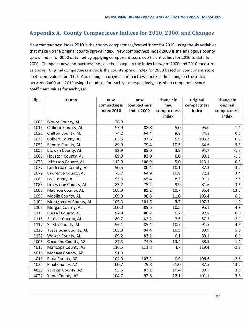
MEASURING URBAN SPRAWL AND VALIDATING SPRAWL MEASURES
91
Appendix A. County Compactness Indices for 2010, 2000, and Changes
New compactness index 2010 is the county compactness/sprawl index for 2010, using the six variables
that make up the original county sprawl index. New compactness index 2000 is the analogous county
sprawl index for 2000 obtained by applying component score coefficient values for 2010 to data for
2000. Change in new compactness index is the change in the index between 2000 and 2010 measured
as above. Original compactness index is the county sprawl index for 2000 based on component score
coefficient values for 2000. And change in original compactness index is the change in the index
between 2000 and 2010 using the indices for each year respectively, based on component score
coefficient values for each year.
fips county new compactness index 2010
new compactness index 2000
change in new
compactness index
original compactness
index
change in original
compactness index
1009 Blount County, AL 76.9 1015 Calhoun County, AL 93.9 88.8 5.0 95.0 -1.1
1021 Chilton County, AL 74.2 64.4 9.8 74.1 0.1
1033 Colbert County, AL 103.6 97.6 5.9 103.2 0.3
1051 Elmore County, AL 89.9 79.4 10.5 84.6 5.3
1055 Etowah County, AL 92.9 89.0 3.9 94.7 -1.8
1069 Houston County, AL 89.0 83.0 6.0 90.1 -1.1
1073 Jefferson County, AL 113.9 108.9 5.0 113.1 0.8
1077 Lauderdale County, AL 90.5 80.4 10.1 87.3 3.2
1079 Lawrence County, AL 75.7 64.9 10.8 72.2 3.4
1081 Lee County, AL 93.6 85.4 8.3 91.1 2.5
1083 Limestone County, AL 85.2 75.2 9.9 81.6 3.6
1089 Madison County, AL 108.9 89.2 19.7 95.4 13.5
1097 Mobile County, AL 109.9 98.8 11.0 103.4 6.5
1101 Montgomery County, AL 105.3 101.6 3.7 107.3 -1.9
1103 Morgan County, AL 100.0 89.6 10.5 95.1 4.9
1113 Russell County, AL 92.9 86.2 6.7 92.8 0.1
1115 St. Clair County, AL 89.7 82.2 7.5 87.5 2.1
1117 Shelby County, AL 96.1 85.4 10.7 91.5 4.6
1125 Tuscaloosa County, AL 105.0 94.4 10.5 99.9 5.0
1127 Walker County, AL 89.2 83.1 6.1 89.1 0.1
4005 Coconino County, AZ 87.3 74.0 13.4 88.5 -1.1
4013 Maricopa County, AZ 116.5 111.8 4.7 119.4 -2.8
4015 Mohave County, AZ 91.3 4019 Pima County, AZ 104.0 103.2 0.9 106.6 -2.6
4021 Pinal County, AZ 100.7 79.8 21.0 87.5 13.2
4025 Yavapai County, AZ 93.5 83.1 10.4 90.5 3.1
4027 Yuma County, AZ 104.7 92.6 12.1 101.1 3.6
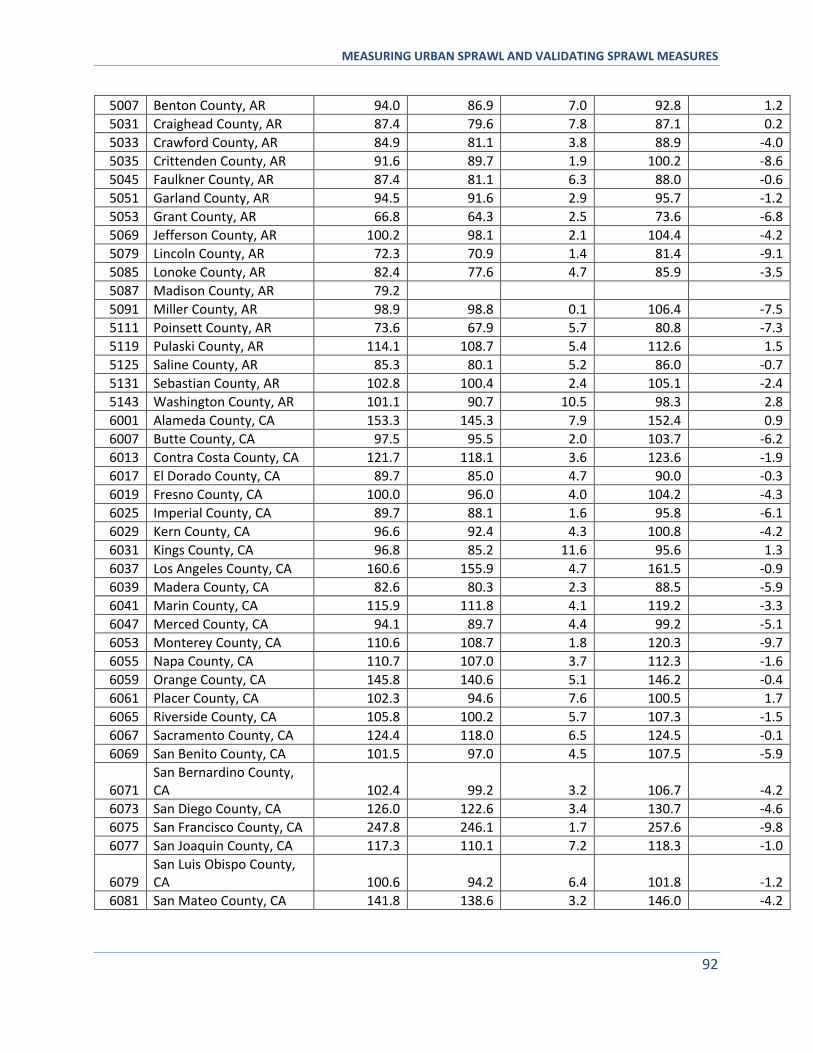
MEASURING URBAN SPRAWL AND VALIDATING SPRAWL MEASURES
92
5007 Benton County, AR 94.0 86.9 7.0 92.8 1.2
5031 Craighead County, AR 87.4 79.6 7.8 87.1 0.2
5033 Crawford County, AR 84.9 81.1 3.8 88.9 -4.0
5035 Crittenden County, AR 91.6 89.7 1.9 100.2 -8.6
5045 Faulkner County, AR 87.4 81.1 6.3 88.0 -0.6
5051 Garland County, AR 94.5 91.6 2.9 95.7 -1.2
5053 Grant County, AR 66.8 64.3 2.5 73.6 -6.8
5069 Jefferson County, AR 100.2 98.1 2.1 104.4 -4.2
5079 Lincoln County, AR 72.3 70.9 1.4 81.4 -9.1
5085 Lonoke County, AR 82.4 77.6 4.7 85.9 -3.5
5087 Madison County, AR 79.2 5091 Miller County, AR 98.9 98.8 0.1 106.4 -7.5
5111 Poinsett County, AR 73.6 67.9 5.7 80.8 -7.3
5119 Pulaski County, AR 114.1 108.7 5.4 112.6 1.5
5125 Saline County, AR 85.3 80.1 5.2 86.0 -0.7
5131 Sebastian County, AR 102.8 100.4 2.4 105.1 -2.4
5143 Washington County, AR 101.1 90.7 10.5 98.3 2.8
6001 Alameda County, CA 153.3 145.3 7.9 152.4 0.9
6007 Butte County, CA 97.5 95.5 2.0 103.7 -6.2
6013 Contra Costa County, CA 121.7 118.1 3.6 123.6 -1.9
6017 El Dorado County, CA 89.7 85.0 4.7 90.0 -0.3
6019 Fresno County, CA 100.0 96.0 4.0 104.2 -4.3
6025 Imperial County, CA 89.7 88.1 1.6 95.8 -6.1
6029 Kern County, CA 96.6 92.4 4.3 100.8 -4.2
6031 Kings County, CA 96.8 85.2 11.6 95.6 1.3
6037 Los Angeles County, CA 160.6 155.9 4.7 161.5 -0.9
6039 Madera County, CA 82.6 80.3 2.3 88.5 -5.9
6041 Marin County, CA 115.9 111.8 4.1 119.2 -3.3
6047 Merced County, CA 94.1 89.7 4.4 99.2 -5.1
6053 Monterey County, CA 110.6 108.7 1.8 120.3 -9.7
6055 Napa County, CA 110.7 107.0 3.7 112.3 -1.6
6059 Orange County, CA 145.8 140.6 5.1 146.2 -0.4
6061 Placer County, CA 102.3 94.6 7.6 100.5 1.7
6065 Riverside County, CA 105.8 100.2 5.7 107.3 -1.5
6067 Sacramento County, CA 124.4 118.0 6.5 124.5 -0.1
6069 San Benito County, CA 101.5 97.0 4.5 107.5 -5.9
6071 San Bernardino County, CA 102.4 99.2 3.2 106.7 -4.2
6073 San Diego County, CA 126.0 122.6 3.4 130.7 -4.6
6075 San Francisco County, CA 247.8 246.1 1.7 257.6 -9.8
6077 San Joaquin County, CA 117.3 110.1 7.2 118.3 -1.0
6079 San Luis Obispo County, CA 100.6 94.2 6.4 101.8 -1.2
6081 San Mateo County, CA 141.8 138.6 3.2 146.0 -4.2
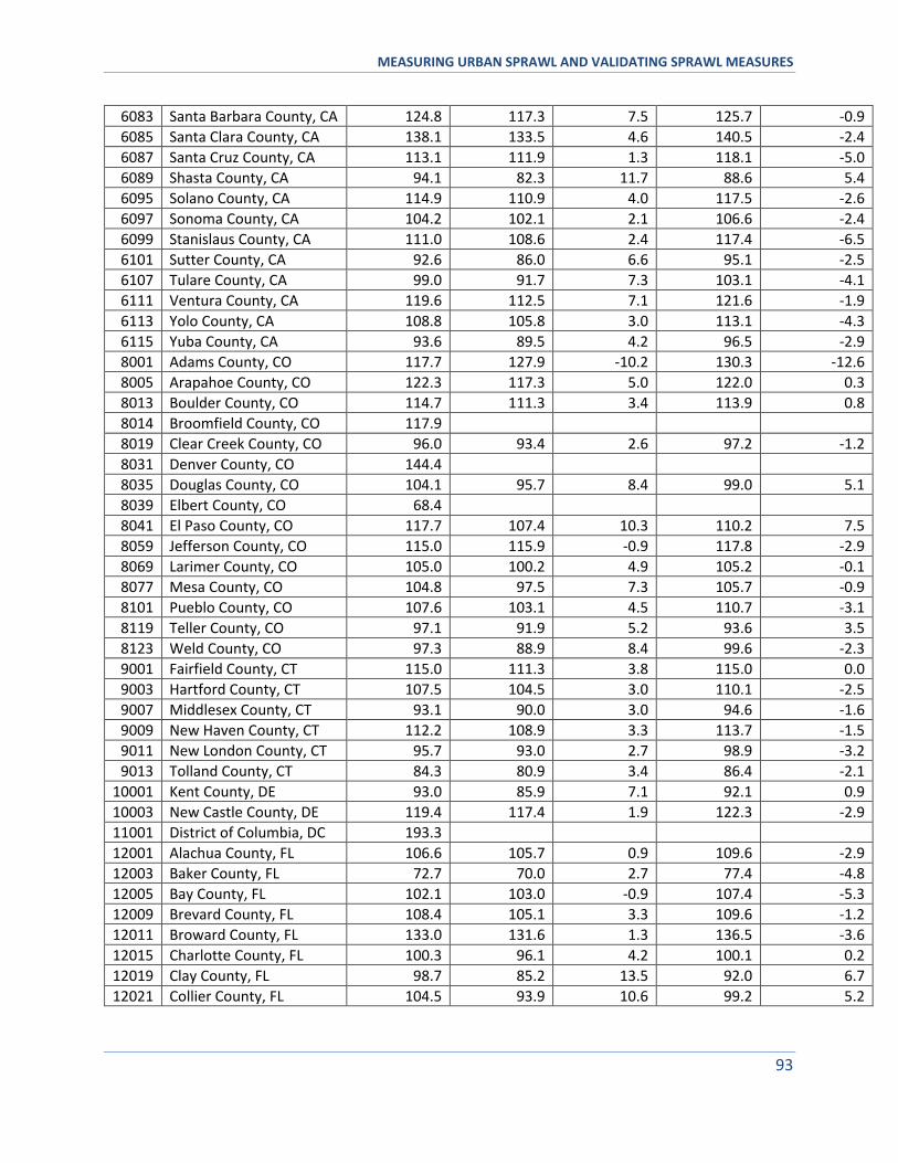
MEASURING URBAN SPRAWL AND VALIDATING SPRAWL MEASURES
93
6083 Santa Barbara County, CA 124.8 117.3 7.5 125.7 -0.9
6085 Santa Clara County, CA 138.1 133.5 4.6 140.5 -2.4
6087 Santa Cruz County, CA 113.1 111.9 1.3 118.1 -5.0
6089 Shasta County, CA 94.1 82.3 11.7 88.6 5.4
6095 Solano County, CA 114.9 110.9 4.0 117.5 -2.6
6097 Sonoma County, CA 104.2 102.1 2.1 106.6 -2.4
6099 Stanislaus County, CA 111.0 108.6 2.4 117.4 -6.5
6101 Sutter County, CA 92.6 86.0 6.6 95.1 -2.5
6107 Tulare County, CA 99.0 91.7 7.3 103.1 -4.1
6111 Ventura County, CA 119.6 112.5 7.1 121.6 -1.9
6113 Yolo County, CA 108.8 105.8 3.0 113.1 -4.3
6115 Yuba County, CA 93.6 89.5 4.2 96.5 -2.9
8001 Adams County, CO 117.7 127.9 -10.2 130.3 -12.6
8005 Arapahoe County, CO 122.3 117.3 5.0 122.0 0.3
8013 Boulder County, CO 114.7 111.3 3.4 113.9 0.8
8014 Broomfield County, CO 117.9 8019 Clear Creek County, CO 96.0 93.4 2.6 97.2 -1.2
8031 Denver County, CO 144.4 8035 Douglas County, CO 104.1 95.7 8.4 99.0 5.1
8039 Elbert County, CO 68.4 8041 El Paso County, CO 117.7 107.4 10.3 110.2 7.5
8059 Jefferson County, CO 115.0 115.9 -0.9 117.8 -2.9
8069 Larimer County, CO 105.0 100.2 4.9 105.2 -0.1
8077 Mesa County, CO 104.8 97.5 7.3 105.7 -0.9
8101 Pueblo County, CO 107.6 103.1 4.5 110.7 -3.1
8119 Teller County, CO 97.1 91.9 5.2 93.6 3.5
8123 Weld County, CO 97.3 88.9 8.4 99.6 -2.3
9001 Fairfield County, CT 115.0 111.3 3.8 115.0 0.0
9003 Hartford County, CT 107.5 104.5 3.0 110.1 -2.5
9007 Middlesex County, CT 93.1 90.0 3.0 94.6 -1.6
9009 New Haven County, CT 112.2 108.9 3.3 113.7 -1.5
9011 New London County, CT 95.7 93.0 2.7 98.9 -3.2
9013 Tolland County, CT 84.3 80.9 3.4 86.4 -2.1
10001 Kent County, DE 93.0 85.9 7.1 92.1 0.9
10003 New Castle County, DE 119.4 117.4 1.9 122.3 -2.9
11001 District of Columbia, DC 193.3 12001 Alachua County, FL 106.6 105.7 0.9 109.6 -2.9
12003 Baker County, FL 72.7 70.0 2.7 77.4 -4.8
12005 Bay County, FL 102.1 103.0 -0.9 107.4 -5.3
12009 Brevard County, FL 108.4 105.1 3.3 109.6 -1.2
12011 Broward County, FL 133.0 131.6 1.3 136.5 -3.6
12015 Charlotte County, FL 100.3 96.1 4.2 100.1 0.2
12019 Clay County, FL 98.7 85.2 13.5 92.0 6.7
12021 Collier County, FL 104.5 93.9 10.6 99.2 5.2
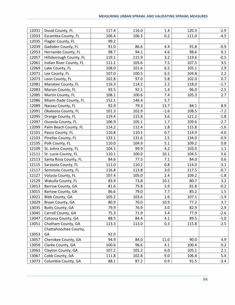
MEASURING URBAN SPRAWL AND VALIDATING SPRAWL MEASURES
94
12031 Duval County, FL 117.4 116.0 1.4 120.3 -2.9
12033 Escambia County, FL 106.4 106.3 0.2 111.0 -4.5
12035 Flagler County, FL 99.2 12039 Gadsden County, FL 91.0 86.6 4.4 91.8 -0.9
12053 Hernando County, FL 98.7 94.1 4.6 98.6 0.1
12057 Hillsborough County, FL 119.1 115.9 3.2 119.6 -0.5
12061 Indian River County, FL 111.1 103.6 7.5 107.5 3.5
12069 Lake County, FL 108.0 101.6 6.5 105.1 2.9
12071 Lee County, FL 107.0 100.5 6.5 104.8 2.2
12073 Leon County, FL 102.8 97.0 5.8 102.0 0.7
12081 Manatee County, FL 116.3 114.2 2.2 118.0 -1.7
12083 Marion County, FL 93.5 92.1 1.4 96.0 -2.5
12085 Martin County, FL 108.1 100.6 7.4 105.3 2.7
12086 Miami-Dade County, FL 152.1 146.4 5.7 12089 Nassau County, FL 92.9 79.3 13.7 84.1 8.9
12091 Okaloosa County, FL 101.3 102.9 -1.6 108.5 -7.2
12095 Orange County, FL 119.4 115.8 3.6 121.2 -1.8
12097 Osceola County, FL 106.9 105.1 1.7 109.6 -2.7
12099 Palm Beach County, FL 114.2 112.4 1.8 115.8 -1.6
12101 Pasco County, FL 110.8 110.1 0.7 114.9 -4.0
12103 Pinellas County, FL 133.1 131.6 1.5 134.0 -0.9
12105 Polk County, FL 110.0 104.9 5.1 109.2 0.8
12109 St. Johns County, FL 104.1 99.9 4.2 103.0 1.1
12111 St. Lucie County, FL 110.1 100.0 10.1 104.5 5.6
12113 Santa Rosa County, FL 84.6 77.5 7.1 84.0 0.6
12115 Sarasota County, FL 111.0 110.2 0.8 114.0 -3.1
12117 Seminole County, FL 116.8 113.8 3.0 117.5 -0.7
12127 Volusia County, FL 107.4 105.0 2.4 109.2 -1.8
12129 Wakulla County, FL 83.9 73.8 10.1 80.7 3.2
13013 Barrow County, GA 81.6 75.8 5.9 81.8 -0.2
13015 Bartow County, GA 86.6 79.0 7.7 85.2 1.5
13021 Bibb County, GA 105.2 103.6 1.6 107.1 -1.9
13029 Bryan County, GA 80.9 70.0 10.9 77.2 3.7
13035 Butts County, GA 79.9 76.9 3.0 82.9 -2.9
13045 Carroll County, GA 75.3 71.9 3.4 77.9 -2.6
13047 Catoosa County, GA 88.5 84.4 4.1 89.5 -1.0
13051 Chatham County, GA 113.3 113.0 0.3 115.8 -2.5
13053 Chattahoochee County, GA 92.0
13057 Cherokee County, GA 94.9 84.0 11.0 90.0 4.9
13059 Clarke County, GA 100.6 96.6 4.1 100.4 0.2
13063 Clayton County, GA 107.2 101.2 6.0 105.1 2.1
13067 Cobb County, GA 111.8 102.8 9.0 106.4 5.4
13073 Columbia County, GA 88.1 87.2 0.9 91.5 -3.4
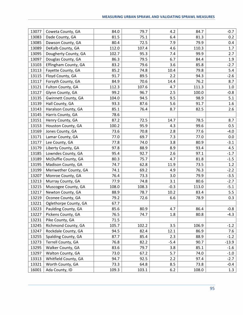
MEASURING URBAN SPRAWL AND VALIDATING SPRAWL MEASURES
95
13077 Coweta County, GA 84.0 79.7 4.2 84.7 -0.7
13083 Dade County, GA 81.5 75.1 6.4 81.3 0.2
13085 Dawson County, GA 80.4 72.5 7.9 79.9 0.4
13089 DeKalb County, GA 112.0 107.4 4.6 110.3 1.7
13095 Dougherty County, GA 102.7 95.3 7.4 99.9 2.7
13097 Douglas County, GA 86.3 79.5 6.7 84.4 1.9
13103 Effingham County, GA 83.2 79.6 3.6 85.8 -2.7
13113 Fayette County, GA 85.2 74.8 10.4 79.8 5.4
13115 Floyd County, GA 91.7 89.5 2.2 94.3 -2.6
13117 Forsyth County, GA 84.9 70.6 14.4 76.2 8.7
13121 Fulton County, GA 112.3 107.6 4.7 111.3 1.0
13127 Glynn County, GA 99.2 96.7 2.5 100.0 -0.8
13135 Gwinnett County, GA 104.0 94.5 9.5 98.9 5.1
13139 Hall County, GA 93.3 87.6 5.6 91.7 1.6
13143 Haralson County, GA 85.1 76.4 8.7 82.5 2.6
13145 Harris County, GA 78.6 13151 Henry County, GA 87.2 72.5 14.7 78.5 8.7
13153 Houston County, GA 100.2 95.9 4.3 99.6 0.5
13169 Jones County, GA 73.6 70.8 2.8 77.6 -4.0
13171 Lamar County, GA 77.0 69.7 7.3 77.0 0.0
13177 Lee County, GA 77.8 74.0 3.8 80.9 -3.1
13179 Liberty County, GA 97.8 88.9 8.9 93.4 4.5
13185 Lowndes County, GA 95.4 92.7 2.6 97.1 -1.7
13189 McDuffie County, GA 80.3 75.7 4.7 81.8 -1.5
13195 Madison County, GA 74.7 62.8 11.9 73.5 1.2
13199 Meriwether County, GA 74.1 69.2 4.9 76.3 -2.2
13207 Monroe County, GA 76.4 73.3 3.0 79.9 -3.5
13213 Murray County, GA 77.9 74.8 3.1 80.6 -2.7
13215 Muscogee County, GA 108.0 108.3 -0.3 113.0 -5.1
13217 Newton County, GA 88.9 78.7 10.2 83.4 5.5
13219 Oconee County, GA 79.2 72.6 6.6 78.9 0.3
13221 Oglethorpe County, GA 67.7 13223 Paulding County, GA 85.6 80.9 4.7 86.4 -0.8
13227 Pickens County, GA 76.5 74.7 1.8 80.8 -4.3
13231 Pike County, GA 71.5 13245 Richmond County, GA 105.7 102.2 3.5 106.9 -1.2
13247 Rockdale County, GA 94.5 82.4 12.1 86.9 7.6
13255 Spalding County, GA 87.7 85.4 2.3 88.9 -1.2
13273 Terrell County, GA 76.8 82.2 -5.4 90.7 -13.9
13295 Walker County, GA 83.6 79.7 3.8 85.1 -1.6
13297 Walton County, GA 73.0 67.2 5.7 74.0 -1.0
13313 Whitfield County, GA 94.7 92.5 2.2 97.4 -2.7
13321 Worth County, GA 73.3 64.8 8.5 73.8 -0.4
16001 Ada County, ID 109.3 103.1 6.2 108.0 1.3
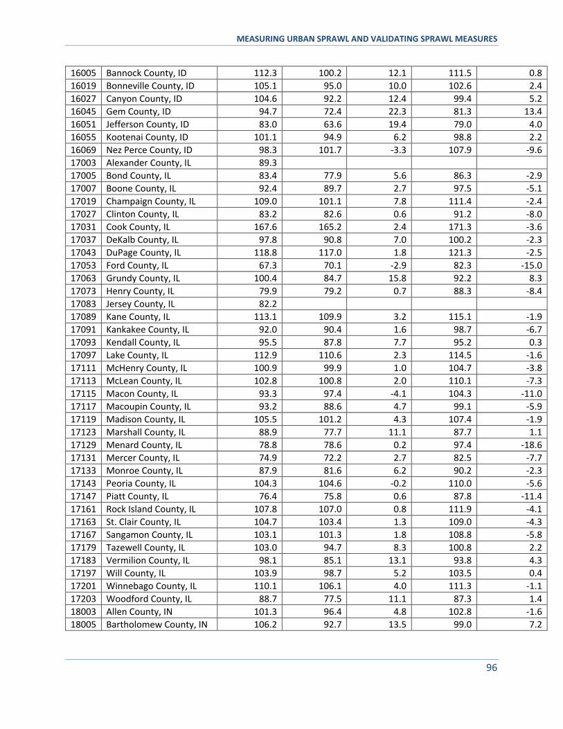
MEASURING URBAN SPRAWL AND VALIDATING SPRAWL MEASURES
96
16005 Bannock County, ID 112.3 100.2 12.1 111.5 0.8
16019 Bonneville County, ID 105.1 95.0 10.0 102.6 2.4
16027 Canyon County, ID 104.6 92.2 12.4 99.4 5.2
16045 Gem County, ID 94.7 72.4 22.3 81.3 13.4
16051 Jefferson County, ID 83.0 63.6 19.4 79.0 4.0
16055 Kootenai County, ID 101.1 94.9 6.2 98.8 2.2
16069 Nez Perce County, ID 98.3 101.7 -3.3 107.9 -9.6
17003 Alexander County, IL 89.3 17005 Bond County, IL 83.4 77.9 5.6 86.3 -2.9
17007 Boone County, IL 92.4 89.7 2.7 97.5 -5.1
17019 Champaign County, IL 109.0 101.1 7.8 111.4 -2.4
17027 Clinton County, IL 83.2 82.6 0.6 91.2 -8.0
17031 Cook County, IL 167.6 165.2 2.4 171.3 -3.6
17037 DeKalb County, IL 97.8 90.8 7.0 100.2 -2.3
17043 DuPage County, IL 118.8 117.0 1.8 121.3 -2.5
17053 Ford County, IL 67.3 70.1 -2.9 82.3 -15.0
17063 Grundy County, IL 100.4 84.7 15.8 92.2 8.3
17073 Henry County, IL 79.9 79.2 0.7 88.3 -8.4
17083 Jersey County, IL 82.2 17089 Kane County, IL 113.1 109.9 3.2 115.1 -1.9
17091 Kankakee County, IL 92.0 90.4 1.6 98.7 -6.7
17093 Kendall County, IL 95.5 87.8 7.7 95.2 0.3
17097 Lake County, IL 112.9 110.6 2.3 114.5 -1.6
17111 McHenry County, IL 100.9 99.9 1.0 104.7 -3.8
17113 McLean County, IL 102.8 100.8 2.0 110.1 -7.3
17115 Macon County, IL 93.3 97.4 -4.1 104.3 -11.0
17117 Macoupin County, IL 93.2 88.6 4.7 99.1 -5.9
17119 Madison County, IL 105.5 101.2 4.3 107.4 -1.9
17123 Marshall County, IL 88.9 77.7 11.1 87.7 1.1
17129 Menard County, IL 78.8 78.6 0.2 97.4 -18.6
17131 Mercer County, IL 74.9 72.2 2.7 82.5 -7.7
17133 Monroe County, IL 87.9 81.6 6.2 90.2 -2.3
17143 Peoria County, IL 104.3 104.6 -0.2 110.0 -5.6
17147 Piatt County, IL 76.4 75.8 0.6 87.8 -11.4
17161 Rock Island County, IL 107.8 107.0 0.8 111.9 -4.1
17163 St. Clair County, IL 104.7 103.4 1.3 109.0 -4.3
17167 Sangamon County, IL 103.1 101.3 1.8 108.8 -5.8
17179 Tazewell County, IL 103.0 94.7 8.3 100.8 2.2
17183 Vermilion County, IL 98.1 85.1 13.1 93.8 4.3
17197 Will County, IL 103.9 98.7 5.2 103.5 0.4
17201 Winnebago County, IL 110.1 106.1 4.0 111.3 -1.1
17203 Woodford County, IL 88.7 77.5 11.1 87.3 1.4
18003 Allen County, IN 101.3 96.4 4.8 102.8 -1.6
18005 Bartholomew County, IN 106.2 92.7 13.5 99.0 7.2
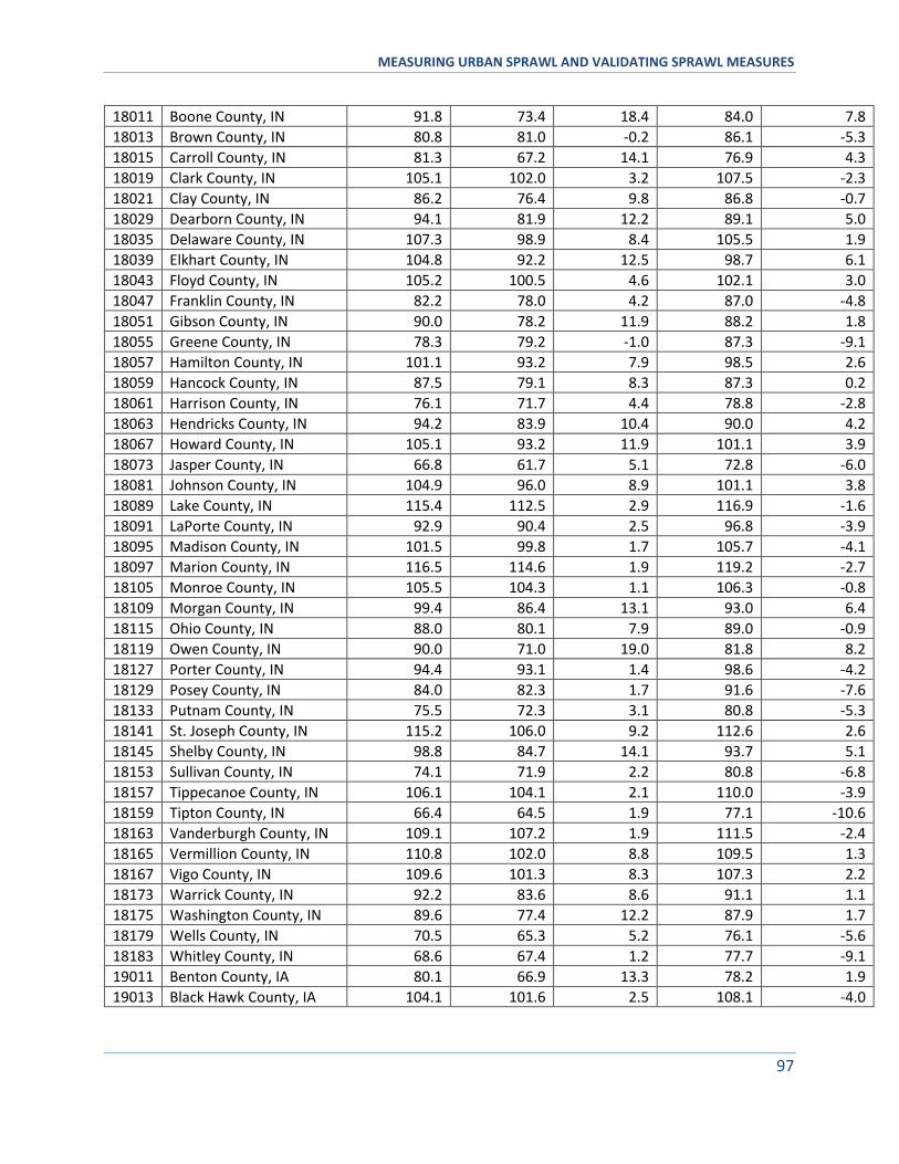
MEASURING URBAN SPRAWL AND VALIDATING SPRAWL MEASURES
97
18011 Boone County, IN 91.8 73.4 18.4 84.0 7.8
18013 Brown County, IN 80.8 81.0 -0.2 86.1 -5.3
18015 Carroll County, IN 81.3 67.2 14.1 76.9 4.3
18019 Clark County, IN 105.1 102.0 3.2 107.5 -2.3
18021 Clay County, IN 86.2 76.4 9.8 86.8 -0.7
18029 Dearborn County, IN 94.1 81.9 12.2 89.1 5.0
18035 Delaware County, IN 107.3 98.9 8.4 105.5 1.9
18039 Elkhart County, IN 104.8 92.2 12.5 98.7 6.1
18043 Floyd County, IN 105.2 100.5 4.6 102.1 3.0
18047 Franklin County, IN 82.2 78.0 4.2 87.0 -4.8
18051 Gibson County, IN 90.0 78.2 11.9 88.2 1.8
18055 Greene County, IN 78.3 79.2 -1.0 87.3 -9.1
18057 Hamilton County, IN 101.1 93.2 7.9 98.5 2.6
18059 Hancock County, IN 87.5 79.1 8.3 87.3 0.2
18061 Harrison County, IN 76.1 71.7 4.4 78.8 -2.8
18063 Hendricks County, IN 94.2 83.9 10.4 90.0 4.2
18067 Howard County, IN 105.1 93.2 11.9 101.1 3.9
18073 Jasper County, IN 66.8 61.7 5.1 72.8 -6.0
18081 Johnson County, IN 104.9 96.0 8.9 101.1 3.8
18089 Lake County, IN 115.4 112.5 2.9 116.9 -1.6
18091 LaPorte County, IN 92.9 90.4 2.5 96.8 -3.9
18095 Madison County, IN 101.5 99.8 1.7 105.7 -4.1
18097 Marion County, IN 116.5 114.6 1.9 119.2 -2.7
18105 Monroe County, IN 105.5 104.3 1.1 106.3 -0.8
18109 Morgan County, IN 99.4 86.4 13.1 93.0 6.4
18115 Ohio County, IN 88.0 80.1 7.9 89.0 -0.9
18119 Owen County, IN 90.0 71.0 19.0 81.8 8.2
18127 Porter County, IN 94.4 93.1 1.4 98.6 -4.2
18129 Posey County, IN 84.0 82.3 1.7 91.6 -7.6
18133 Putnam County, IN 75.5 72.3 3.1 80.8 -5.3
18141 St. Joseph County, IN 115.2 106.0 9.2 112.6 2.6
18145 Shelby County, IN 98.8 84.7 14.1 93.7 5.1
18153 Sullivan County, IN 74.1 71.9 2.2 80.8 -6.8
18157 Tippecanoe County, IN 106.1 104.1 2.1 110.0 -3.9
18159 Tipton County, IN 66.4 64.5 1.9 77.1 -10.6
18163 Vanderburgh County, IN 109.1 107.2 1.9 111.5 -2.4
18165 Vermillion County, IN 110.8 102.0 8.8 109.5 1.3
18167 Vigo County, IN 109.6 101.3 8.3 107.3 2.2
18173 Warrick County, IN 92.2 83.6 8.6 91.1 1.1
18175 Washington County, IN 89.6 77.4 12.2 87.9 1.7
18179 Wells County, IN 70.5 65.3 5.2 76.1 -5.6
18183 Whitley County, IN 68.6 67.4 1.2 77.7 -9.1
19011 Benton County, IA 80.1 66.9 13.3 78.2 1.9
19013 Black Hawk County, IA 104.1 101.6 2.5 108.1 -4.0
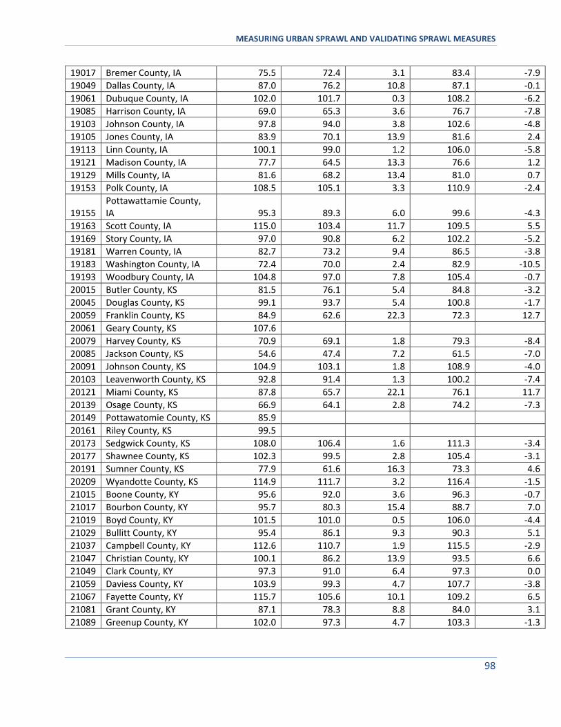
MEASURING URBAN SPRAWL AND VALIDATING SPRAWL MEASURES
98
19017 Bremer County, IA 75.5 72.4 3.1 83.4 -7.9
19049 Dallas County, IA 87.0 76.2 10.8 87.1 -0.1
19061 Dubuque County, IA 102.0 101.7 0.3 108.2 -6.2
19085 Harrison County, IA 69.0 65.3 3.6 76.7 -7.8
19103 Johnson County, IA 97.8 94.0 3.8 102.6 -4.8
19105 Jones County, IA 83.9 70.1 13.9 81.6 2.4
19113 Linn County, IA 100.1 99.0 1.2 106.0 -5.8
19121 Madison County, IA 77.7 64.5 13.3 76.6 1.2
19129 Mills County, IA 81.6 68.2 13.4 81.0 0.7
19153 Polk County, IA 108.5 105.1 3.3 110.9 -2.4
19155 Pottawattamie County, IA 95.3 89.3 6.0 99.6 -4.3
19163 Scott County, IA 115.0 103.4 11.7 109.5 5.5
19169 Story County, IA 97.0 90.8 6.2 102.2 -5.2
19181 Warren County, IA 82.7 73.2 9.4 86.5 -3.8
19183 Washington County, IA 72.4 70.0 2.4 82.9 -10.5
19193 Woodbury County, IA 104.8 97.0 7.8 105.4 -0.7
20015 Butler County, KS 81.5 76.1 5.4 84.8 -3.2
20045 Douglas County, KS 99.1 93.7 5.4 100.8 -1.7
20059 Franklin County, KS 84.9 62.6 22.3 72.3 12.7
20061 Geary County, KS 107.6 20079 Harvey County, KS 70.9 69.1 1.8 79.3 -8.4
20085 Jackson County, KS 54.6 47.4 7.2 61.5 -7.0
20091 Johnson County, KS 104.9 103.1 1.8 108.9 -4.0
20103 Leavenworth County, KS 92.8 91.4 1.3 100.2 -7.4
20121 Miami County, KS 87.8 65.7 22.1 76.1 11.7
20139 Osage County, KS 66.9 64.1 2.8 74.2 -7.3
20149 Pottawatomie County, KS 85.9 20161 Riley County, KS 99.5 20173 Sedgwick County, KS 108.0 106.4 1.6 111.3 -3.4
20177 Shawnee County, KS 102.3 99.5 2.8 105.4 -3.1
20191 Sumner County, KS 77.9 61.6 16.3 73.3 4.6
20209 Wyandotte County, KS 114.9 111.7 3.2 116.4 -1.5
21015 Boone County, KY 95.6 92.0 3.6 96.3 -0.7
21017 Bourbon County, KY 95.7 80.3 15.4 88.7 7.0
21019 Boyd County, KY 101.5 101.0 0.5 106.0 -4.4
21029 Bullitt County, KY 95.4 86.1 9.3 90.3 5.1
21037 Campbell County, KY 112.6 110.7 1.9 115.5 -2.9
21047 Christian County, KY 100.1 86.2 13.9 93.5 6.6
21049 Clark County, KY 97.3 91.0 6.4 97.3 0.0
21059 Daviess County, KY 103.9 99.3 4.7 107.7 -3.8
21067 Fayette County, KY 115.7 105.6 10.1 109.2 6.5
21081 Grant County, KY 87.1 78.3 8.8 84.0 3.1
21089 Greenup County, KY 102.0 97.3 4.7 103.3 -1.3
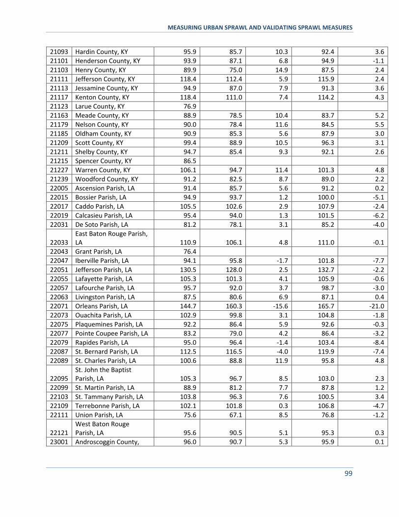
MEASURING URBAN SPRAWL AND VALIDATING SPRAWL MEASURES
99
21093 Hardin County, KY 95.9 85.7 10.3 92.4 3.6
21101 Henderson County, KY 93.9 87.1 6.8 94.9 -1.1
21103 Henry County, KY 89.9 75.0 14.9 87.5 2.4
21111 Jefferson County, KY 118.4 112.4 5.9 115.9 2.4
21113 Jessamine County, KY 94.9 87.0 7.9 91.3 3.6
21117 Kenton County, KY 118.4 111.0 7.4 114.2 4.3
21123 Larue County, KY 76.9 21163 Meade County, KY 88.9 78.5 10.4 83.7 5.2
21179 Nelson County, KY 90.0 78.4 11.6 84.5 5.5
21185 Oldham County, KY 90.9 85.3 5.6 87.9 3.0
21209 Scott County, KY 99.4 88.9 10.5 96.3 3.1
21211 Shelby County, KY 94.7 85.4 9.3 92.1 2.6
21215 Spencer County, KY 86.5 21227 Warren County, KY 106.1 94.7 11.4 101.3 4.8
21239 Woodford County, KY 91.2 82.5 8.7 89.0 2.2
22005 Ascension Parish, LA 91.4 85.7 5.6 91.2 0.2
22015 Bossier Parish, LA 94.9 93.7 1.2 100.0 -5.1
22017 Caddo Parish, LA 105.5 102.6 2.9 107.9 -2.4
22019 Calcasieu Parish, LA 95.4 94.0 1.3 101.5 -6.2
22031 De Soto Parish, LA 81.2 78.1 3.1 85.2 -4.0
22033 East Baton Rouge Parish, LA 110.9 106.1 4.8 111.0 -0.1
22043 Grant Parish, LA 76.4 22047 Iberville Parish, LA 94.1 95.8 -1.7 101.8 -7.7
22051 Jefferson Parish, LA 130.5 128.0 2.5 132.7 -2.2
22055 Lafayette Parish, LA 105.3 101.3 4.1 105.9 -0.6
22057 Lafourche Parish, LA 95.7 92.0 3.7 98.7 -3.0
22063 Livingston Parish, LA 87.5 80.6 6.9 87.1 0.4
22071 Orleans Parish, LA 144.7 160.3 -15.6 165.7 -21.0
22073 Ouachita Parish, LA 102.9 99.8 3.1 104.8 -1.8
22075 Plaquemines Parish, LA 92.2 86.4 5.9 92.6 -0.3
22077 Pointe Coupee Parish, LA 83.2 79.0 4.2 86.4 -3.2
22079 Rapides Parish, LA 95.0 96.4 -1.4 103.4 -8.4
22087 St. Bernard Parish, LA 112.5 116.5 -4.0 119.9 -7.4
22089 St. Charles Parish, LA 100.6 88.8 11.9 95.8 4.8
22095 St. John the Baptist Parish, LA 105.3 96.7 8.5 103.0 2.3
22099 St. Martin Parish, LA 88.9 81.2 7.7 87.8 1.2
22103 St. Tammany Parish, LA 103.8 96.3 7.6 100.5 3.4
22109 Terrebonne Parish, LA 102.1 101.8 0.3 106.8 -4.7
22111 Union Parish, LA 75.6 67.1 8.5 76.8 -1.2
22121 West Baton Rouge Parish, LA 95.6 90.5 5.1 95.3 0.3
23001 Androscoggin County, 96.0 90.7 5.3 95.9 0.1
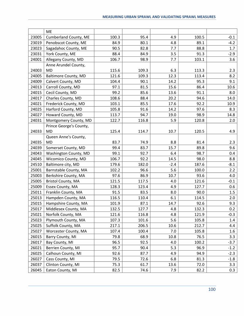
MEASURING URBAN SPRAWL AND VALIDATING SPRAWL MEASURES
100
ME
23005 Cumberland County, ME 100.3 95.4 4.9 100.5 -0.1
23019 Penobscot County, ME 84.9 80.1 4.8 89.1 -4.2
23023 Sagadahoc County, ME 90.5 82.8 7.7 88.8 1.7
23031 York County, ME 88.4 84.9 3.5 91.3 -2.9
24001 Allegany County, MD 106.7 98.9 7.7 103.1 3.6
24003 Anne Arundel County, MD 115.6 109.3 6.3 113.3 2.3
24005 Baltimore County, MD 121.6 109.3 12.3 113.4 8.2
24009 Calvert County, MD 104.4 90.1 14.2 95.3 9.1
24013 Carroll County, MD 97.1 81.5 15.6 86.4 10.6
24015 Cecil County, MD 99.2 85.6 13.6 91.1 8.0
24017 Charles County, MD 108.6 88.4 20.2 94.6 14.0
24021 Frederick County, MD 103.1 85.5 17.6 92.2 10.9
24025 Harford County, MD 105.8 91.6 14.2 97.6 8.3
24027 Howard County, MD 113.7 94.7 19.0 98.9 14.8
24031 Montgomery County, MD 122.7 116.8 5.9 120.8 2.0
24033 Prince George's County, MD 125.4 114.7 10.7 120.5 4.9
24035 Queen Anne's County, MD 83.7 74.9 8.8 81.4 2.3
24039 Somerset County, MD 99.4 83.7 15.7 89.8 9.6
24043 Washington County, MD 99.1 92.7 6.4 98.7 0.4
24045 Wicomico County, MD 106.7 92.2 14.5 98.0 8.8
24510 Baltimore city, MD 179.6 182.0 -2.4 187.6 -8.1
25001 Barnstable County, MA 102.2 96.6 5.6 100.0 2.2
25003 Berkshire County, MA 97.6 86.9 10.7 93.6 4.0
25005 Bristol County, MA 121.5 117.5 4.0 121.6 -0.1
25009 Essex County, MA 128.3 123.4 4.9 127.7 0.6
25011 Franklin County, MA 91.5 83.5 8.0 90.0 1.5
25013 Hampden County, MA 116.5 110.4 6.1 114.5 2.0
25015 Hampshire County, MA 101.9 87.1 14.7 92.6 9.3
25017 Middlesex County, MA 132.5 127.7 4.8 132.3 0.2
25021 Norfolk County, MA 121.6 116.8 4.8 121.9 -0.3
25023 Plymouth County, MA 107.3 101.6 5.6 105.8 1.4
25025 Suffolk County, MA 217.1 206.5 10.6 212.7 4.4
25027 Worcester County, MA 107.4 100.4 7.0 105.8 1.6
26015 Barry County, MI 79.8 68.9 10.8 76.5 3.3
26017 Bay County, MI 96.5 92.5 4.0 100.2 -3.7
26021 Berrien County, MI 95.7 90.4 5.3 96.9 -1.2
26025 Calhoun County, MI 92.6 87.7 4.9 94.9 -2.3
26027 Cass County, MI 79.5 72.6 6.8 81.3 -1.8
26037 Clinton County, MI 75.3 61.7 13.6 72.0 3.3
26045 Eaton County, MI 82.5 74.6 7.9 82.2 0.3
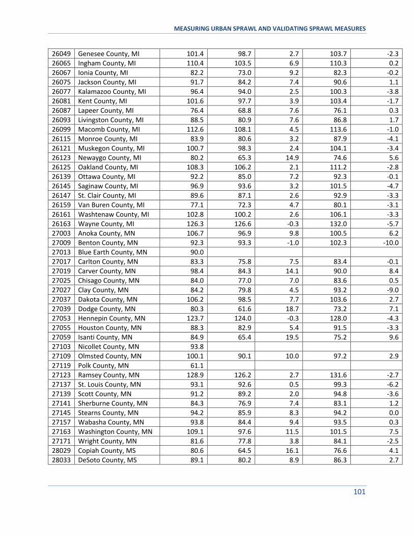
MEASURING URBAN SPRAWL AND VALIDATING SPRAWL MEASURES
101
26049 Genesee County, MI 101.4 98.7 2.7 103.7 -2.3
26065 Ingham County, MI 110.4 103.5 6.9 110.3 0.2
26067 Ionia County, MI 82.2 73.0 9.2 82.3 -0.2
26075 Jackson County, MI 91.7 84.2 7.4 90.6 1.1
26077 Kalamazoo County, MI 96.4 94.0 2.5 100.3 -3.8
26081 Kent County, MI 101.6 97.7 3.9 103.4 -1.7
26087 Lapeer County, MI 76.4 68.8 7.6 76.1 0.3
26093 Livingston County, MI 88.5 80.9 7.6 86.8 1.7
26099 Macomb County, MI 112.6 108.1 4.5 113.6 -1.0
26115 Monroe County, MI 83.9 80.6 3.2 87.9 -4.1
26121 Muskegon County, MI 100.7 98.3 2.4 104.1 -3.4
26123 Newaygo County, MI 80.2 65.3 14.9 74.6 5.6
26125 Oakland County, MI 108.3 106.2 2.1 111.2 -2.8
26139 Ottawa County, MI 92.2 85.0 7.2 92.3 -0.1
26145 Saginaw County, MI 96.9 93.6 3.2 101.5 -4.7
26147 St. Clair County, MI 89.6 87.1 2.6 92.9 -3.3
26159 Van Buren County, MI 77.1 72.3 4.7 80.1 -3.1
26161 Washtenaw County, MI 102.8 100.2 2.6 106.1 -3.3
26163 Wayne County, MI 126.3 126.6 -0.3 132.0 -5.7
27003 Anoka County, MN 106.7 96.9 9.8 100.5 6.2
27009 Benton County, MN 92.3 93.3 -1.0 102.3 -10.0
27013 Blue Earth County, MN 90.0 27017 Carlton County, MN 83.3 75.8 7.5 83.4 -0.1
27019 Carver County, MN 98.4 84.3 14.1 90.0 8.4
27025 Chisago County, MN 84.0 77.0 7.0 83.6 0.5
27027 Clay County, MN 84.2 79.8 4.5 93.2 -9.0
27037 Dakota County, MN 106.2 98.5 7.7 103.6 2.7
27039 Dodge County, MN 80.3 61.6 18.7 73.2 7.1
27053 Hennepin County, MN 123.7 124.0 -0.3 128.0 -4.3
27055 Houston County, MN 88.3 82.9 5.4 91.5 -3.3
27059 Isanti County, MN 84.9 65.4 19.5 75.2 9.6
27103 Nicollet County, MN 93.8 27109 Olmsted County, MN 100.1 90.1 10.0 97.2 2.9
27119 Polk County, MN 61.1 27123 Ramsey County, MN 128.9 126.2 2.7 131.6 -2.7
27137 St. Louis County, MN 93.1 92.6 0.5 99.3 -6.2
27139 Scott County, MN 91.2 89.2 2.0 94.8 -3.6
27141 Sherburne County, MN 84.3 76.9 7.4 83.1 1.2
27145 Stearns County, MN 94.2 85.9 8.3 94.2 0.0
27157 Wabasha County, MN 93.8 84.4 9.4 93.5 0.3
27163 Washington County, MN 109.1 97.6 11.5 101.5 7.5
27171 Wright County, MN 81.6 77.8 3.8 84.1 -2.5
28029 Copiah County, MS 80.6 64.5 16.1 76.6 4.1
28033 DeSoto County, MS 89.1 80.2 8.9 86.3 2.7
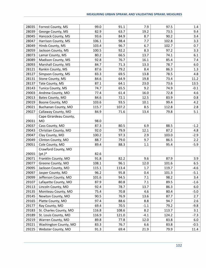
MEASURING URBAN SPRAWL AND VALIDATING SPRAWL MEASURES
102
28035 Forrest County, MS 99.0 91.1 7.9 97.5 1.4
28039 George County, MS 82.9 63.7 19.2 73.5 9.4
28045 Hancock County, MS 93.6 84.9 8.7 90.2 3.4
28047 Harrison County, MS 106.1 98.4 7.7 102.8 3.3
28049 Hinds County, MS 103.4 96.7 6.7 102.7 0.7
28059 Jackson County, MS 100.5 92.2 8.3 97.2 3.3
28073 Lamar County, MS 80.2 66.5 13.7 74.1 6.1
28089 Madison County, MS 92.8 76.7 16.1 85.4 7.4
28093 Marshall County, MS 84.7 71.3 13.3 78.7 6.0
28121 Rankin County, MS 87.6 79.2 8.4 86.3 1.3
28127 Simpson County, MS 83.3 69.5 13.8 78.5 4.8
28131 Stone County, MS 84.6 64.9 19.8 73.4 11.2
28137 Tate County, MS 87.1 64.1 23.0 73.6 13.5
28143 Tunica County, MS 74.7 65.5 9.2 74.9 -0.1
29003 Andrew County, MO 77.4 61.4 16.0 72.8 4.6
29013 Bates County, MO 84.6 72.1 12.5 83.9 0.8
29019 Boone County, MO 103.6 93.5 10.1 99.4 4.2
29021 Buchanan County, MO 115.7 107.2 8.5 112.8 2.8
29027 Callaway County, MO 84.9 71.6 13.4 79.8 5.1
29031 Cape Girardeau County, MO 98.0
29037 Cass County, MO 87.3 80.5 6.9 88.5 -1.2
29043 Christian County, MO 92.0 79.9 12.1 87.2 4.8
29047 Clay County, MO 100.2 97.3 2.9 103.0 -2.9
29049 Clinton County, MO 88.7 79.0 9.7 86.5 2.2
29051 Cole County, MO 89.4 88.3 1.1 95.4 -5.9
29055 Crawford County, MO (pt.)* 82.6
29071 Franklin County, MO 91.8 82.2 9.6 87.9 3.9
29077 Greene County, MO 108.1 96.1 12.0 101.6 6.5
29095 Jackson County, MO 115.1 113.4 1.7 119.7 -4.6
29097 Jasper County, MO 96.2 95.8 0.4 101.3 -5.1
29099 Jefferson County, MO 101.6 94.5 7.1 98.2 3.4
29107 Lafayette County, MO 87.9 80.8 7.1 89.5 -1.6
29113 Lincoln County, MO 92.4 78.7 13.7 86.3 6.0
29135 Moniteau County, MO 75.4 70.8 4.6 80.4 -5.0
29145 Newton County, MO 90.5 76.9 13.6 87.7 2.7
29165 Platte County, MO 97.4 88.6 8.8 94.7 2.6
29177 Ray County, MO 69.4 70.5 -1.1 79.2 -9.8
29183 St. Charles County, MO 116.8 108.6 8.2 113.7 3.1
29189 St. Louis County, MO 116.9 121.0 -4.1 124.2 -7.3
29219 Warren County, MO 89.8 77.8 12.0 83.8 6.0
29221 Washington County, MO 83.3 76.7 6.6 83.8 -0.5
29225 Webster County, MO 91.3 69.4 21.9 79.9 11.4
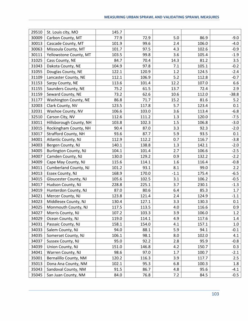
MEASURING URBAN SPRAWL AND VALIDATING SPRAWL MEASURES
103
29510 St. Louis city, MO 145.7 30009 Carbon County, MT 77.9 72.9 5.0 86.9 -9.0
30013 Cascade County, MT 101.9 99.6 2.4 106.0 -4.0
30063 Missoula County, MT 101.7 97.5 4.3 102.6 -0.9
30111 Yellowstone County, MT 103.5 99.8 3.6 105.4 -1.9
31025 Cass County, NE 84.7 70.4 14.3 81.2 3.5
31043 Dakota County, NE 104.9 97.8 7.1 105.1 -0.2
31055 Douglas County, NE 122.1 120.9 1.2 124.5 -2.4
31109 Lancaster County, NE 112.1 106.9 5.2 112.8 -0.7
31153 Sarpy County, NE 113.6 101.4 12.2 107.0 6.6
31155 Saunders County, NE 75.2 61.5 13.7 72.4 2.9
31159 Seward County, NE 73.2 62.6 10.6 112.0 -38.8
31177 Washington County, NE 86.8 71.7 15.2 81.6 5.2
32003 Clark County, NV 123.5 117.8 5.7 123.4 0.1
32031 Washoe County, NV 106.6 103.0 3.6 113.4 -6.8
32510 Carson City, NV 112.6 111.2 1.3 120.0 -7.5
33011 Hillsborough County, NH 103.8 102.3 1.5 106.8 -3.0
33015 Rockingham County, NH 90.4 87.0 3.3 92.3 -2.0
33017 Strafford County, NH 93.6 87.7 5.9 93.5 0.1
34001 Atlantic County, NJ 112.9 112.2 0.7 116.7 -3.8
34003 Bergen County, NJ 140.1 138.8 1.3 142.1 -2.0
34005 Burlington County, NJ 104.1 101.4 2.7 106.6 -2.5
34007 Camden County, NJ 130.0 129.2 0.9 132.2 -2.2
34009 Cape May County, NJ 115.6 114.1 1.6 116.4 -0.8
34011 Cumberland County, NJ 101.2 93.1 8.1 99.0 2.2
34013 Essex County, NJ 168.9 170.0 -1.1 175.4 -6.5
34015 Gloucester County, NJ 105.6 102.5 3.1 106.2 -0.5
34017 Hudson County, NJ 228.8 225.1 3.7 230.1 -1.3
34019 Hunterdon County, NJ 87.0 80.6 6.4 85.3 1.7
34021 Mercer County, NJ 123.8 121.4 2.4 124.9 -1.1
34023 Middlesex County, NJ 130.4 127.1 3.3 130.3 0.1
34025 Monmouth County, NJ 117.5 113.5 4.0 116.6 0.9
34027 Morris County, NJ 107.2 103.3 3.9 106.0 1.2
34029 Ocean County, NJ 119.0 114.1 4.9 117.6 1.4
34031 Passaic County, NJ 158.1 154.0 4.1 157.1 1.0
34033 Salem County, NJ 94.0 88.1 5.9 94.1 -0.1
34035 Somerset County, NJ 106.1 98.1 8.0 102.0 4.1
34037 Sussex County, NJ 95.0 92.2 2.8 95.9 -0.8
34039 Union County, NJ 151.0 146.8 4.2 150.7 0.3
34041 Warren County, NJ 98.6 97.0 1.7 100.7 -2.1
35001 Bernalillo County, NM 120.2 116.3 3.9 117.7 2.5
35013 Dona Ana County, NM 102.1 95.3 6.8 100.3 1.8
35043 Sandoval County, NM 91.5 86.7 4.8 95.6 -4.1
35045 San Juan County, NM 84.0 76.8 7.2 84.5 -0.5
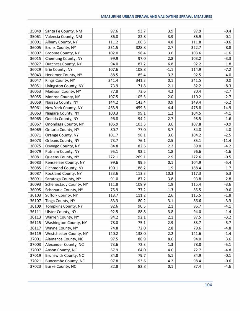
MEASURING URBAN SPRAWL AND VALIDATING SPRAWL MEASURES
104
35049 Santa Fe County, NM 97.6 93.7 3.9 97.9 -0.4
35061 Valencia County, NM 86.8 82.8 3.9 86.9 -0.1
36001 Albany County, NY 111.2 106.5 4.8 111.8 -0.6
36005 Bronx County, NY 331.5 328.8 2.7 322.7 8.8
36007 Broome County, NY 102.0 98.4 3.6 103.6 -1.6
36015 Chemung County, NY 99.9 97.0 2.8 103.2 -3.3
36027 Dutchess County, NY 94.0 87.2 6.8 92.2 1.8
36029 Erie County, NY 107.6 108.8 -1.1 114.9 -7.2
36043 Herkimer County, NY 88.5 85.4 3.2 92.5 -4.0
36047 Kings County, NY 341.4 341.3 0.1 341.5 0.0
36051 Livingston County, NY 73.9 71.8 2.1 82.2 -8.3
36053 Madison County, NY 77.8 73.6 4.2 80.4 -2.7
36055 Monroe County, NY 107.5 105.5 2.0 110.2 -2.7
36059 Nassau County, NY 144.2 143.4 0.9 149.4 -5.2
36061 New York County, NY 463.9 459.5 4.4 478.8 -14.9
36063 Niagara County, NY 100.3 99.1 1.2 104.5 -4.1
36065 Oneida County, NY 96.8 94.2 2.7 98.5 -1.6
36067 Onondaga County, NY 106.9 103.3 3.6 107.8 -0.9
36069 Ontario County, NY 80.7 77.0 3.7 84.8 -4.0
36071 Orange County, NY 101.7 98.1 3.6 104.2 -2.5
36073 Orleans County, NY 73.7 76.1 -2.5 85.1 -11.4
36075 Oswego County, NY 84.8 82.6 2.2 89.0 -4.2
36079 Putnam County, NY 95.1 93.2 1.8 96.6 -1.6
36081 Queens County, NY 272.1 269.1 2.9 272.6 -0.5
36083 Rensselaer County, NY 99.6 99.5 0.1 104.9 -5.4
36085 Richmond County, NY 190.1 188.2 1.9 188.4 1.7
36087 Rockland County, NY 123.6 113.3 10.3 117.3 6.3
36091 Saratoga County, NY 91.0 87.2 3.8 93.8 -2.8
36093 Schenectady County, NY 111.8 109.9 1.9 115.4 -3.6
36095 Schoharie County, NY 75.9 77.2 -1.3 85.5 -9.6
36103 Suffolk County, NY 113.7 111.2 2.6 115.5 -1.8
36107 Tioga County, NY 83.3 80.2 3.1 86.6 -3.3
36109 Tompkins County, NY 92.6 90.5 2.1 96.7 -4.1
36111 Ulster County, NY 92.5 88.8 3.8 94.0 -1.4
36113 Warren County, NY 94.2 92.1 2.1 97.5 -3.2
36115 Washington County, NY 78.0 75.1 2.9 83.7 -5.7
36117 Wayne County, NY 74.8 72.0 2.8 79.6 -4.8
36119 Westchester County, NY 140.2 138.0 2.2 141.6 -1.4
37001 Alamance County, NC 97.5 88.9 8.6 94.0 3.6
37003 Alexander County, NC 73.6 72.3 1.3 78.8 -5.1
37007 Anson County, NC 67.9 64.0 4.0 72.7 -4.8
37019 Brunswick County, NC 84.8 79.7 5.1 84.9 -0.1
37021 Buncombe County, NC 97.8 93.6 4.2 98.4 -0.6
37023 Burke County, NC 82.8 82.8 0.1 87.4 -4.6
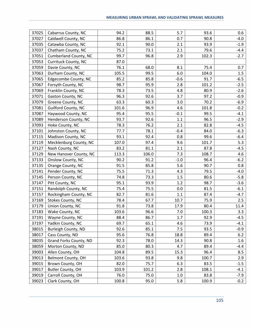
MEASURING URBAN SPRAWL AND VALIDATING SPRAWL MEASURES
105
37025 Cabarrus County, NC 94.2 88.5 5.7 93.6 0.6
37027 Caldwell County, NC 86.8 86.1 0.7 90.8 -4.0
37035 Catawba County, NC 92.1 90.0 2.1 93.9 -1.9
37037 Chatham County, NC 75.2 73.1 2.1 79.6 -4.4
37051 Cumberland County, NC 99.7 96.8 2.9 102.3 -2.7
37053 Currituck County, NC 87.0 37059 Davie County, NC 76.1 68.0 8.1 75.4 0.7
37063 Durham County, NC 105.5 99.5 6.0 104.0 1.5
37065 Edgecombe County, NC 85.2 85.8 -0.6 91.7 -6.5
37067 Forsyth County, NC 98.7 95.9 2.8 101.2 -2.5
37069 Franklin County, NC 78.3 73.5 4.8 80.9 -2.6
37071 Gaston County, NC 96.3 92.6 3.7 97.2 -0.9
37079 Greene County, NC 63.3 60.3 3.0 70.2 -6.9
37081 Guilford County, NC 101.6 96.9 4.6 101.8 -0.2
37087 Haywood County, NC 95.4 95.5 -0.1 99.5 -4.1
37089 Henderson County, NC 93.7 92.6 1.1 96.5 -2.9
37093 Hoke County, NC 78.3 76.2 2.1 82.8 -4.5
37101 Johnston County, NC 77.7 78.1 -0.4 84.0 -6.3
37115 Madison County, NC 93.1 92.4 0.8 99.6 -6.4
37119 Mecklenburg County, NC 107.0 97.4 9.6 101.7 5.3
37127 Nash County, NC 83.2 81.1 2.1 87.8 -4.5
37129 New Hanover County, NC 113.3 106.0 7.3 108.7 4.6
37133 Onslow County, NC 90.2 91.2 -1.0 96.4 -6.2
37135 Orange County, NC 91.5 85.8 5.6 90.7 0.8
37141 Pender County, NC 75.5 71.3 4.3 79.5 -4.0
37145 Person County, NC 74.8 73.3 1.5 80.6 -5.8
37147 Pitt County, NC 95.1 93.9 1.2 98.7 -3.6
37151 Randolph County, NC 75.4 75.5 0.0 81.5 -6.1
37157 Rockingham County, NC 82.7 81.6 1.1 87.4 -4.7
37169 Stokes County, NC 78.4 67.7 10.7 75.9 2.5
37179 Union County, NC 91.8 73.8 17.9 80.4 11.4
37183 Wake County, NC 103.6 96.6 7.0 100.3 3.3
37191 Wayne County, NC 88.4 86.7 1.7 92.9 -4.5
37197 Yadkin County, NC 69.7 65.1 4.6 73.9 -4.1
38015 Burleigh County, ND 92.6 85.1 7.5 93.5 -0.9
38017 Cass County, ND 95.6 76.8 18.8 89.4 6.2
38035 Grand Forks County, ND 92.3 78.0 14.3 90.8 1.6
38059 Morton County, ND 85.0 80.3 4.7 89.4 -4.4
39003 Allen County, OH 104.8 89.5 15.3 96.4 8.5
39013 Belmont County, OH 103.6 93.8 9.8 100.7 2.9
39015 Brown County, OH 82.0 75.7 6.3 83.5 -1.5
39017 Butler County, OH 103.9 101.2 2.8 108.1 -4.1
39019 Carroll County, OH 76.0 75.0 1.0 83.8 -7.9
39023 Clark County, OH 100.8 95.0 5.8 100.9 -0.2
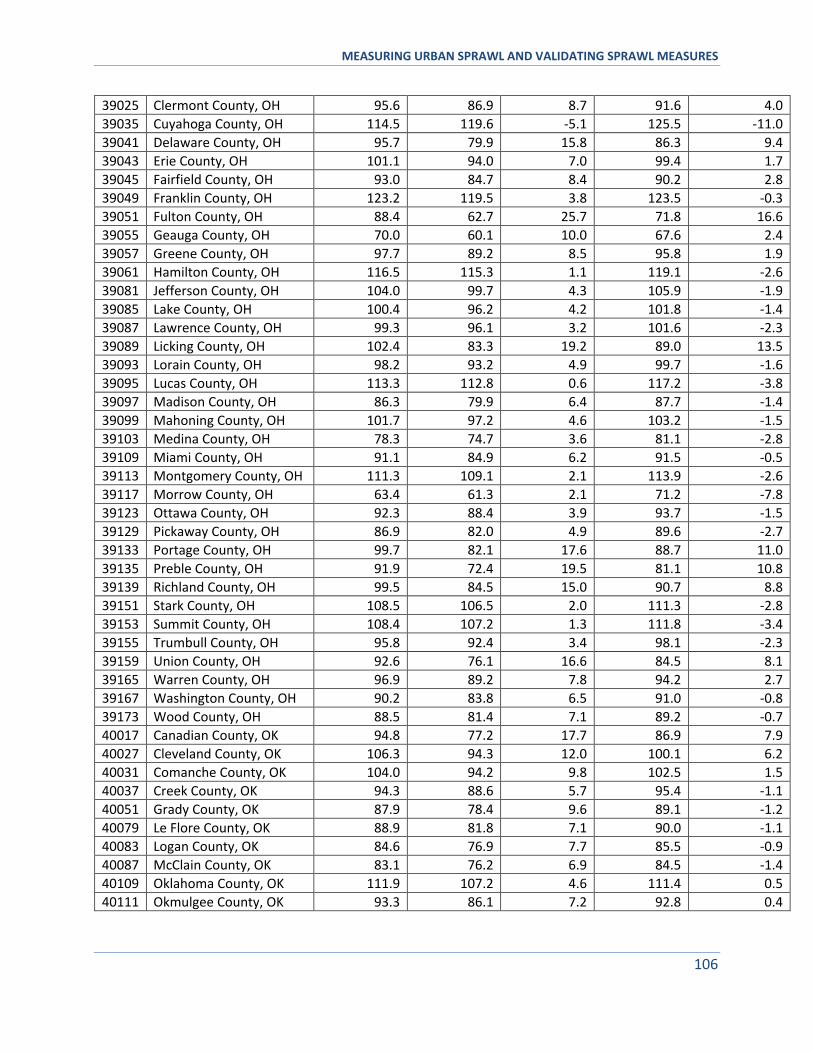
MEASURING URBAN SPRAWL AND VALIDATING SPRAWL MEASURES
106
39025 Clermont County, OH 95.6 86.9 8.7 91.6 4.0
39035 Cuyahoga County, OH 114.5 119.6 -5.1 125.5 -11.0
39041 Delaware County, OH 95.7 79.9 15.8 86.3 9.4
39043 Erie County, OH 101.1 94.0 7.0 99.4 1.7
39045 Fairfield County, OH 93.0 84.7 8.4 90.2 2.8
39049 Franklin County, OH 123.2 119.5 3.8 123.5 -0.3
39051 Fulton County, OH 88.4 62.7 25.7 71.8 16.6
39055 Geauga County, OH 70.0 60.1 10.0 67.6 2.4
39057 Greene County, OH 97.7 89.2 8.5 95.8 1.9
39061 Hamilton County, OH 116.5 115.3 1.1 119.1 -2.6
39081 Jefferson County, OH 104.0 99.7 4.3 105.9 -1.9
39085 Lake County, OH 100.4 96.2 4.2 101.8 -1.4
39087 Lawrence County, OH 99.3 96.1 3.2 101.6 -2.3
39089 Licking County, OH 102.4 83.3 19.2 89.0 13.5
39093 Lorain County, OH 98.2 93.2 4.9 99.7 -1.6
39095 Lucas County, OH 113.3 112.8 0.6 117.2 -3.8
39097 Madison County, OH 86.3 79.9 6.4 87.7 -1.4
39099 Mahoning County, OH 101.7 97.2 4.6 103.2 -1.5
39103 Medina County, OH 78.3 74.7 3.6 81.1 -2.8
39109 Miami County, OH 91.1 84.9 6.2 91.5 -0.5
39113 Montgomery County, OH 111.3 109.1 2.1 113.9 -2.6
39117 Morrow County, OH 63.4 61.3 2.1 71.2 -7.8
39123 Ottawa County, OH 92.3 88.4 3.9 93.7 -1.5
39129 Pickaway County, OH 86.9 82.0 4.9 89.6 -2.7
39133 Portage County, OH 99.7 82.1 17.6 88.7 11.0
39135 Preble County, OH 91.9 72.4 19.5 81.1 10.8
39139 Richland County, OH 99.5 84.5 15.0 90.7 8.8
39151 Stark County, OH 108.5 106.5 2.0 111.3 -2.8
39153 Summit County, OH 108.4 107.2 1.3 111.8 -3.4
39155 Trumbull County, OH 95.8 92.4 3.4 98.1 -2.3
39159 Union County, OH 92.6 76.1 16.6 84.5 8.1
39165 Warren County, OH 96.9 89.2 7.8 94.2 2.7
39167 Washington County, OH 90.2 83.8 6.5 91.0 -0.8
39173 Wood County, OH 88.5 81.4 7.1 89.2 -0.7
40017 Canadian County, OK 94.8 77.2 17.7 86.9 7.9
40027 Cleveland County, OK 106.3 94.3 12.0 100.1 6.2
40031 Comanche County, OK 104.0 94.2 9.8 102.5 1.5
40037 Creek County, OK 94.3 88.6 5.7 95.4 -1.1
40051 Grady County, OK 87.9 78.4 9.6 89.1 -1.2
40079 Le Flore County, OK 88.9 81.8 7.1 90.0 -1.1
40083 Logan County, OK 84.6 76.9 7.7 85.5 -0.9
40087 McClain County, OK 83.1 76.2 6.9 84.5 -1.4
40109 Oklahoma County, OK 111.9 107.2 4.6 111.4 0.5
40111 Okmulgee County, OK 93.3 86.1 7.2 92.8 0.4
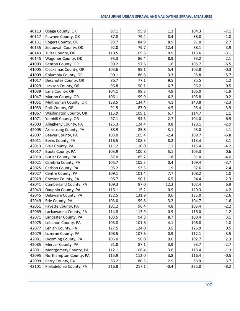
MEASURING URBAN SPRAWL AND VALIDATING SPRAWL MEASURES
107
40113 Osage County, OK 97.1 95.9 1.2 104.3 -7.1
40117 Pawnee County, OK 87.8 79.4 8.4 88.8 -1.0
40131 Rogers County, OK 93.7 84.9 8.9 91.0 2.7
40135 Sequoyah County, OK 92.0 79.7 12.4 88.1 3.9
40143 Tulsa County, OK 110.5 109.6 0.9 113.6 -3.1
40145 Wagoner County, OK 95.3 86.4 8.9 93.2 2.1
41003 Benton County, OR 99.2 97.6 1.6 105.7 -6.5
41005 Clackamas County, OR 103.6 98.1 5.4 103.8 -0.3
41009 Columbia County, OR 90.1 86.8 3.3 95.8 -5.7
41017 Deschutes County, OR 86.7 77.1 9.5 85.5 1.2
41029 Jackson County, OR 96.8 90.1 6.7 96.2 0.5
41039 Lane County, OR 104.1 99.2 4.9 106.0 -1.9
41047 Marion County, OR 106.1 99.9 6.2 105.8 0.2
41051 Multnomah County, OR 138.5 134.4 4.1 140.8 -2.3
41053 Polk County, OR 91.5 87.0 4.5 95.4 -3.9
41067 Washington County, OR 115.9 109.1 6.7 114.7 1.1
41071 Yamhill County, OR 97.1 94.5 2.7 104.0 -6.9
42003 Allegheny County, PA 125.3 124.4 0.8 128.1 -2.9
42005 Armstrong County, PA 88.9 85.8 3.1 93.0 -4.1
42007 Beaver County, PA 103.0 105.4 -2.4 109.7 -6.8
42011 Berks County, PA 116.5 108.3 8.2 113.4 3.1
42013 Blair County, PA 111.2 110.0 1.1 115.4 -4.2
42017 Bucks County, PA 105.9 100.8 5.1 105.3 0.6
42019 Butler County, PA 87.0 85.2 1.8 91.0 -4.0
42021 Cambria County, PA 105.7 105.3 0.4 109.4 -3.7
42025 Carbon County, PA 95.2 93.3 1.9 97.6 -2.4
42027 Centre County, PA 109.1 101.4 7.7 108.2 1.0
42029 Chester County, PA 96.7 90.1 6.5 94.4 2.3
42041 Cumberland County, PA 109.3 97.0 12.3 102.4 6.9
42043 Dauphin County, PA 116.1 115.2 0.9 120.3 -4.2
42045 Delaware County, PA 132.5 131.9 0.6 135.0 -2.6
42049 Erie County, PA 103.0 99.8 3.2 104.7 -1.6
42051 Fayette County, PA 101.2 96.4 4.8 103.4 -2.2
42069 Lackawanna County, PA 114.8 113.9 0.9 116.0 -1.2
42071 Lancaster County, PA 103.5 94.8 8.7 100.4 3.1
42075 Lebanon County, PA 105.8 101.6 4.1 106.8 -1.0
42077 Lehigh County, PA 127.5 124.0 3.5 126.9 0.5
42079 Luzerne County, PA 108.5 107.6 0.9 112.1 -3.5
42081 Lycoming County, PA 105.0 96.0 9.0 102.7 2.3
42085 Mercer County, PA 91.0 87.1 3.9 93.7 -2.7
42091 Montgomery County, PA 112.1 108.4 3.6 113.4 -1.3
42095 Northampton County, PA 115.9 112.0 3.8 116.4 -0.5
42099 Perry County, PA 83.2 80.3 2.9 86.9 -3.7
42101 Philadelphia County, PA 216.8 217.1 -0.4 225.0 -8.2
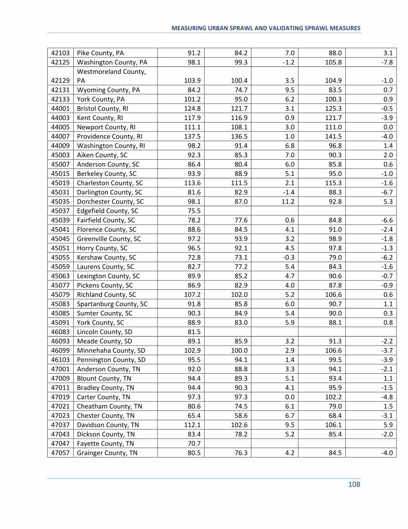
MEASURING URBAN SPRAWL AND VALIDATING SPRAWL MEASURES
108
42103 Pike County, PA 91.2 84.2 7.0 88.0 3.1
42125 Washington County, PA 98.1 99.3 -1.2 105.8 -7.8
42129 Westmoreland County, PA 103.9 100.4 3.5 104.9 -1.0
42131 Wyoming County, PA 84.2 74.7 9.5 83.5 0.7
42133 York County, PA 101.2 95.0 6.2 100.3 0.9
44001 Bristol County, RI 124.8 121.7 3.1 125.3 -0.5
44003 Kent County, RI 117.9 116.9 0.9 121.7 -3.9
44005 Newport County, RI 111.1 108.1 3.0 111.0 0.0
44007 Providence County, RI 137.5 136.5 1.0 141.5 -4.0
44009 Washington County, RI 98.2 91.4 6.8 96.8 1.4
45003 Aiken County, SC 92.3 85.3 7.0 90.3 2.0
45007 Anderson County, SC 86.4 80.4 6.0 85.8 0.6
45015 Berkeley County, SC 93.9 88.9 5.1 95.0 -1.0
45019 Charleston County, SC 113.6 111.5 2.1 115.3 -1.6
45031 Darlington County, SC 81.6 82.9 -1.4 88.3 -6.7
45035 Dorchester County, SC 98.1 87.0 11.2 92.8 5.3
45037 Edgefield County, SC 75.5 45039 Fairfield County, SC 78.2 77.6 0.6 84.8 -6.6
45041 Florence County, SC 88.6 84.5 4.1 91.0 -2.4
45045 Greenville County, SC 97.2 93.9 3.2 98.9 -1.8
45051 Horry County, SC 96.5 92.1 4.5 97.8 -1.3
45055 Kershaw County, SC 72.8 73.1 -0.3 79.0 -6.2
45059 Laurens County, SC 82.7 77.2 5.4 84.3 -1.6
45063 Lexington County, SC 89.9 85.2 4.7 90.6 -0.7
45077 Pickens County, SC 86.9 82.9 4.0 87.8 -0.9
45079 Richland County, SC 107.2 102.0 5.2 106.6 0.6
45083 Spartanburg County, SC 91.8 85.8 6.0 90.7 1.1
45085 Sumter County, SC 90.3 84.9 5.4 90.0 0.3
45091 York County, SC 88.9 83.0 5.9 88.1 0.8
46083 Lincoln County, SD 81.5 46093 Meade County, SD 89.1 85.9 3.2 91.3 -2.2
46099 Minnehaha County, SD 102.9 100.0 2.9 106.6 -3.7
46103 Pennington County, SD 95.5 94.1 1.4 99.5 -3.9
47001 Anderson County, TN 92.0 88.8 3.3 94.1 -2.1
47009 Blount County, TN 94.4 89.3 5.1 93.4 1.1
47011 Bradley County, TN 94.4 90.3 4.1 95.9 -1.5
47019 Carter County, TN 97.3 97.3 0.0 102.2 -4.8
47021 Cheatham County, TN 80.6 74.5 6.1 79.0 1.5
47023 Chester County, TN 65.4 58.6 6.7 68.4 -3.1
47037 Davidson County, TN 112.1 102.6 9.5 106.1 5.9
47043 Dickson County, TN 83.4 78.2 5.2 85.4 -2.0
47047 Fayette County, TN 70.7 47057 Grainger County, TN 80.5 76.3 4.2 84.5 -4.0
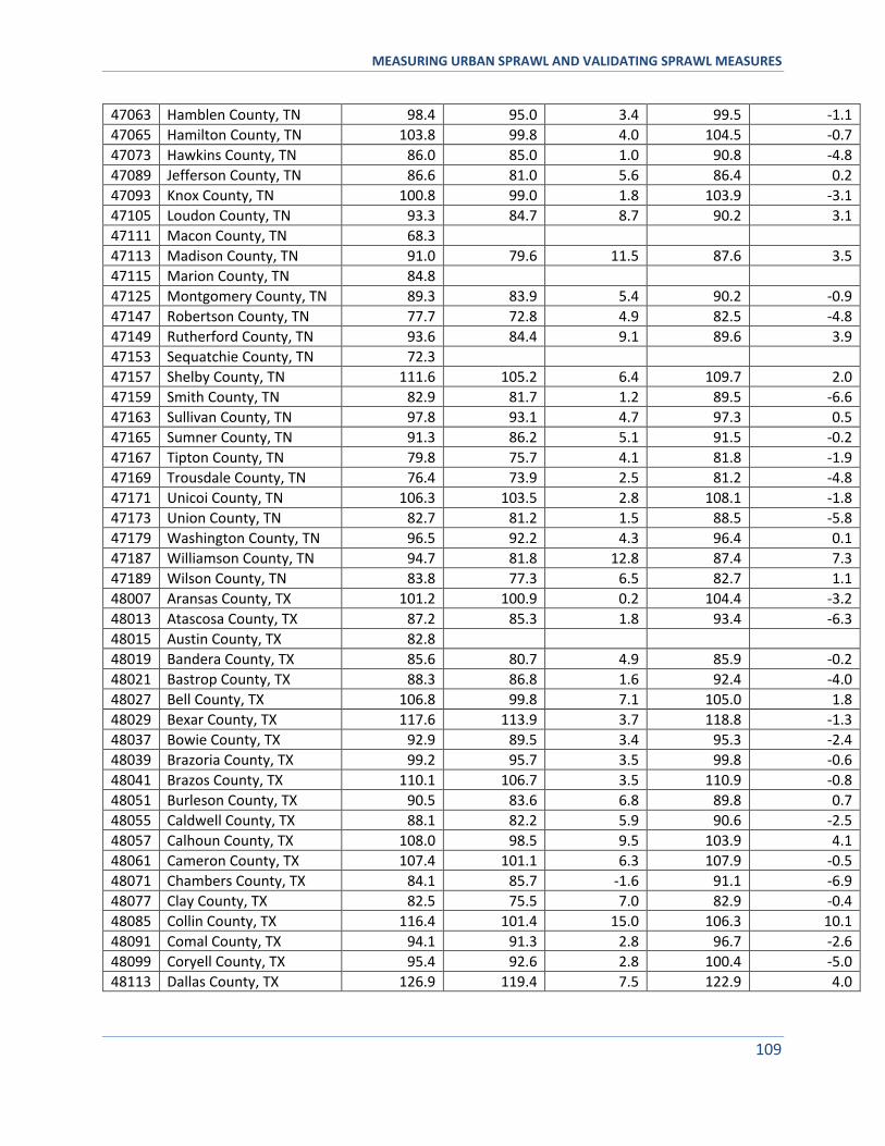
MEASURING URBAN SPRAWL AND VALIDATING SPRAWL MEASURES
109
47063 Hamblen County, TN 98.4 95.0 3.4 99.5 -1.1
47065 Hamilton County, TN 103.8 99.8 4.0 104.5 -0.7
47073 Hawkins County, TN 86.0 85.0 1.0 90.8 -4.8
47089 Jefferson County, TN 86.6 81.0 5.6 86.4 0.2
47093 Knox County, TN 100.8 99.0 1.8 103.9 -3.1
47105 Loudon County, TN 93.3 84.7 8.7 90.2 3.1
47111 Macon County, TN 68.3 47113 Madison County, TN 91.0 79.6 11.5 87.6 3.5
47115 Marion County, TN 84.8 47125 Montgomery County, TN 89.3 83.9 5.4 90.2 -0.9
47147 Robertson County, TN 77.7 72.8 4.9 82.5 -4.8
47149 Rutherford County, TN 93.6 84.4 9.1 89.6 3.9
47153 Sequatchie County, TN 72.3 47157 Shelby County, TN 111.6 105.2 6.4 109.7 2.0
47159 Smith County, TN 82.9 81.7 1.2 89.5 -6.6
47163 Sullivan County, TN 97.8 93.1 4.7 97.3 0.5
47165 Sumner County, TN 91.3 86.2 5.1 91.5 -0.2
47167 Tipton County, TN 79.8 75.7 4.1 81.8 -1.9
47169 Trousdale County, TN 76.4 73.9 2.5 81.2 -4.8
47171 Unicoi County, TN 106.3 103.5 2.8 108.1 -1.8
47173 Union County, TN 82.7 81.2 1.5 88.5 -5.8
47179 Washington County, TN 96.5 92.2 4.3 96.4 0.1
47187 Williamson County, TN 94.7 81.8 12.8 87.4 7.3
47189 Wilson County, TN 83.8 77.3 6.5 82.7 1.1
48007 Aransas County, TX 101.2 100.9 0.2 104.4 -3.2
48013 Atascosa County, TX 87.2 85.3 1.8 93.4 -6.3
48015 Austin County, TX 82.8 48019 Bandera County, TX 85.6 80.7 4.9 85.9 -0.2
48021 Bastrop County, TX 88.3 86.8 1.6 92.4 -4.0
48027 Bell County, TX 106.8 99.8 7.1 105.0 1.8
48029 Bexar County, TX 117.6 113.9 3.7 118.8 -1.3
48037 Bowie County, TX 92.9 89.5 3.4 95.3 -2.4
48039 Brazoria County, TX 99.2 95.7 3.5 99.8 -0.6
48041 Brazos County, TX 110.1 106.7 3.5 110.9 -0.8
48051 Burleson County, TX 90.5 83.6 6.8 89.8 0.7
48055 Caldwell County, TX 88.1 82.2 5.9 90.6 -2.5
48057 Calhoun County, TX 108.0 98.5 9.5 103.9 4.1
48061 Cameron County, TX 107.4 101.1 6.3 107.9 -0.5
48071 Chambers County, TX 84.1 85.7 -1.6 91.1 -6.9
48077 Clay County, TX 82.5 75.5 7.0 82.9 -0.4
48085 Collin County, TX 116.4 101.4 15.0 106.3 10.1
48091 Comal County, TX 94.1 91.3 2.8 96.7 -2.6
48099 Coryell County, TX 95.4 92.6 2.8 100.4 -5.0
48113 Dallas County, TX 126.9 119.4 7.5 122.9 4.0
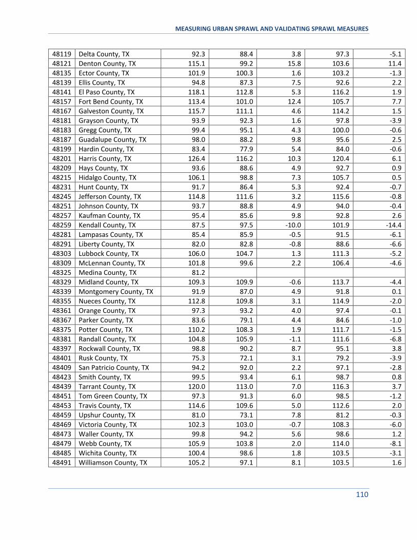
MEASURING URBAN SPRAWL AND VALIDATING SPRAWL MEASURES
110
48119 Delta County, TX 92.3 88.4 3.8 97.3 -5.1
48121 Denton County, TX 115.1 99.2 15.8 103.6 11.4
48135 Ector County, TX 101.9 100.3 1.6 103.2 -1.3
48139 Ellis County, TX 94.8 87.3 7.5 92.6 2.2
48141 El Paso County, TX 118.1 112.8 5.3 116.2 1.9
48157 Fort Bend County, TX 113.4 101.0 12.4 105.7 7.7
48167 Galveston County, TX 115.7 111.1 4.6 114.2 1.5
48181 Grayson County, TX 93.9 92.3 1.6 97.8 -3.9
48183 Gregg County, TX 99.4 95.1 4.3 100.0 -0.6
48187 Guadalupe County, TX 98.0 88.2 9.8 95.6 2.5
48199 Hardin County, TX 83.4 77.9 5.4 84.0 -0.6
48201 Harris County, TX 126.4 116.2 10.3 120.4 6.1
48209 Hays County, TX 93.6 88.6 4.9 92.7 0.9
48215 Hidalgo County, TX 106.1 98.8 7.3 105.7 0.5
48231 Hunt County, TX 91.7 86.4 5.3 92.4 -0.7
48245 Jefferson County, TX 114.8 111.6 3.2 115.6 -0.8
48251 Johnson County, TX 93.7 88.8 4.9 94.0 -0.4
48257 Kaufman County, TX 95.4 85.6 9.8 92.8 2.6
48259 Kendall County, TX 87.5 97.5 -10.0 101.9 -14.4
48281 Lampasas County, TX 85.4 85.9 -0.5 91.5 -6.1
48291 Liberty County, TX 82.0 82.8 -0.8 88.6 -6.6
48303 Lubbock County, TX 106.0 104.7 1.3 111.3 -5.2
48309 McLennan County, TX 101.8 99.6 2.2 106.4 -4.6
48325 Medina County, TX 81.2 48329 Midland County, TX 109.3 109.9 -0.6 113.7 -4.4
48339 Montgomery County, TX 91.9 87.0 4.9 91.8 0.1
48355 Nueces County, TX 112.8 109.8 3.1 114.9 -2.0
48361 Orange County, TX 97.3 93.2 4.0 97.4 -0.1
48367 Parker County, TX 83.6 79.1 4.4 84.6 -1.0
48375 Potter County, TX 110.2 108.3 1.9 111.7 -1.5
48381 Randall County, TX 104.8 105.9 -1.1 111.6 -6.8
48397 Rockwall County, TX 98.8 90.2 8.7 95.1 3.8
48401 Rusk County, TX 75.3 72.1 3.1 79.2 -3.9
48409 San Patricio County, TX 94.2 92.0 2.2 97.1 -2.8
48423 Smith County, TX 99.5 93.4 6.1 98.7 0.8
48439 Tarrant County, TX 120.0 113.0 7.0 116.3 3.7
48451 Tom Green County, TX 97.3 91.3 6.0 98.5 -1.2
48453 Travis County, TX 114.6 109.6 5.0 112.6 2.0
48459 Upshur County, TX 81.0 73.1 7.8 81.2 -0.3
48469 Victoria County, TX 102.3 103.0 -0.7 108.3 -6.0
48473 Waller County, TX 99.8 94.2 5.6 98.6 1.2
48479 Webb County, TX 105.9 103.8 2.0 114.0 -8.1
48485 Wichita County, TX 100.4 98.6 1.8 103.5 -3.1
48491 Williamson County, TX 105.2 97.1 8.1 103.5 1.6
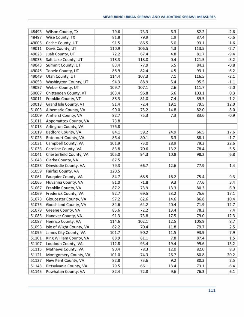
MEASURING URBAN SPRAWL AND VALIDATING SPRAWL MEASURES
111
48493 Wilson County, TX 79.6 73.3 6.3 82.2 -2.6
48497 Wise County, TX 81.8 79.9 1.9 87.4 -5.6
49005 Cache County, UT 91.5 86.5 5.0 93.1 -1.6
49011 Davis County, UT 110.9 106.5 4.3 113.5 -2.7
49023 Juab County, UT 72.2 67.4 4.8 81.7 -9.4
49035 Salt Lake County, UT 118.3 118.0 0.4 121.5 -3.2
49043 Summit County, UT 83.4 77.9 5.5 84.2 -0.8
49045 Tooele County, UT 86.9 82.4 4.5 93.1 -6.2
49049 Utah County, UT 114.4 107.3 7.1 116.5 -2.1
49053 Washington County, UT 94.3 88.9 5.4 95.5 -1.1
49057 Weber County, UT 109.7 107.1 2.6 111.7 -2.0
50007 Chittenden County, VT 103.4 96.8 6.6 103.1 0.3
50011 Franklin County, VT 88.3 81.0 7.4 89.5 -1.2
50013 Grand Isle County, VT 91.4 72.4 19.1 79.5 12.0
51003 Albemarle County, VA 90.0 75.2 14.8 82.0 8.0
51009 Amherst County, VA 82.7 75.3 7.3 83.6 -0.9
51011 Appomattox County, VA 73.8 51013 Arlington County, VA 176.8 51019 Bedford County, VA 84.1 59.2 24.9 66.5 17.6
51023 Botetourt County, VA 86.4 80.1 6.3 88.1 -1.7
51031 Campbell County, VA 101.9 73.0 28.9 79.3 22.6
51033 Caroline County, VA 83.8 70.6 13.2 78.4 5.5
51041 Chesterfield County, VA 105.0 94.3 10.8 98.2 6.8
51043 Clarke County, VA 87.5 51053 Dinwiddie County, VA 79.3 66.7 12.6 77.9 1.4
51059 Fairfax County, VA 120.5 51061 Fauquier County, VA 84.7 68.5 16.2 75.4 9.3
51065 Fluvanna County, VA 81.0 71.8 9.3 77.6 3.4
51067 Franklin County, VA 87.2 73.9 13.3 80.3 6.9
51069 Frederick County, VA 92.7 69.5 23.2 75.6 17.1
51073 Gloucester County, VA 97.2 82.6 14.6 86.8 10.4
51075 Goochland County, VA 84.6 64.2 20.4 71.9 12.7
51079 Greene County, VA 85.6 72.2 13.4 78.2 7.4
51085 Hanover County, VA 91.3 73.8 17.5 79.0 12.3
51087 Henrico County, VA 114.6 102.1 12.5 105.9 8.7
51093 Isle of Wight County, VA 82.2 70.4 11.8 79.7 2.5
51095 James City County, VA 101.7 90.2 11.5 93.9 7.9
51101 King William County, VA 88.9 81.1 7.8 87.4 1.5
51107 Loudoun County, VA 112.8 93.4 19.4 99.6 13.2
51115 Mathews County, VA 90.4 78.3 12.0 82.0 8.3
51121 Montgomery County, VA 101.0 74.3 26.7 80.8 20.2
51127 New Kent County, VA 82.8 73.6 9.2 80.3 2.5
51143 Pittsylvania County, VA 79.5 66.1 13.4 73.1 6.4
51145 Powhatan County, VA 82.4 72.8 9.6 76.3 6.1
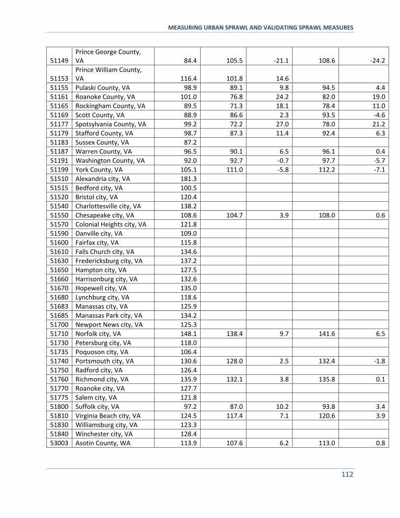
MEASURING URBAN SPRAWL AND VALIDATING SPRAWL MEASURES
112
51149 Prince George County, VA 84.4 105.5 -21.1 108.6 -24.2
51153 Prince William County, VA 116.4 101.8 14.6
51155 Pulaski County, VA 98.9 89.1 9.8 94.5 4.4
51161 Roanoke County, VA 101.0 76.8 24.2 82.0 19.0
51165 Rockingham County, VA 89.5 71.3 18.1 78.4 11.0
51169 Scott County, VA 88.9 86.6 2.3 93.5 -4.6
51177 Spotsylvania County, VA 99.2 72.2 27.0 78.0 21.2
51179 Stafford County, VA 98.7 87.3 11.4 92.4 6.3
51183 Sussex County, VA 87.2 51187 Warren County, VA 96.5 90.1 6.5 96.1 0.4
51191 Washington County, VA 92.0 92.7 -0.7 97.7 -5.7
51199 York County, VA 105.1 111.0 -5.8 112.2 -7.1
51510 Alexandria city, VA 181.3 51515 Bedford city, VA 100.5 51520 Bristol city, VA 120.4 51540 Charlottesville city, VA 138.2 51550 Chesapeake city, VA 108.6 104.7 3.9 108.0 0.6
51570 Colonial Heights city, VA 121.8 51590 Danville city, VA 109.0 51600 Fairfax city, VA 115.8 51610 Falls Church city, VA 134.6 51630 Fredericksburg city, VA 137.2 51650 Hampton city, VA 127.5 51660 Harrisonburg city, VA 132.6 51670 Hopewell city, VA 135.0 51680 Lynchburg city, VA 118.6 51683 Manassas city, VA 125.9 51685 Manassas Park city, VA 134.2 51700 Newport News city, VA 125.3 51710 Norfolk city, VA 148.1 138.4 9.7 141.6 6.5
51730 Petersburg city, VA 118.0 51735 Poquoson city, VA 106.4 51740 Portsmouth city, VA 130.6 128.0 2.5 132.4 -1.8
51750 Radford city, VA 126.4 51760 Richmond city, VA 135.9 132.1 3.8 135.8 0.1
51770 Roanoke city, VA 127.7 51775 Salem city, VA 121.8 51800 Suffolk city, VA 97.2 87.0 10.2 93.8 3.4
51810 Virginia Beach city, VA 124.5 117.4 7.1 120.6 3.9
51830 Williamsburg city, VA 123.3 51840 Winchester city, VA 128.4 53003 Asotin County, WA 113.9 107.6 6.2 113.0 0.8
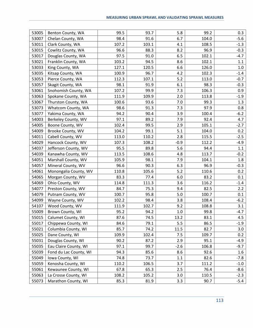
MEASURING URBAN SPRAWL AND VALIDATING SPRAWL MEASURES
113
53005 Benton County, WA 99.5 93.7 5.8 99.2 0.3
53007 Chelan County, WA 98.4 91.6 6.7 104.0 -5.6
53011 Clark County, WA 107.2 103.1 4.1 108.5 -1.3
53015 Cowlitz County, WA 96.6 88.3 8.2 96.9 -0.3
53017 Douglas County, WA 97.5 91.0 6.5 102.1 -4.7
53021 Franklin County, WA 103.2 94.5 8.6 102.1 1.1
53033 King County, WA 127.1 120.5 6.6 126.0 1.0
53035 Kitsap County, WA 100.9 96.7 4.2 102.3 -1.4
53053 Pierce County, WA 112.3 107.1 5.2 113.0 -0.7
53057 Skagit County, WA 98.1 91.9 6.1 98.3 -0.3
53061 Snohomish County, WA 107.2 99.9 7.3 106.3 0.9
53063 Spokane County, WA 111.9 109.9 2.0 113.8 -1.9
53067 Thurston County, WA 100.6 93.6 7.0 99.3 1.3
53073 Whatcom County, WA 98.6 91.3 7.3 97.9 0.8
53077 Yakima County, WA 94.2 90.4 3.9 100.4 -6.2
54003 Berkeley County, WV 97.1 89.2 7.9 92.4 4.7
54005 Boone County, WV 102.4 99.5 2.9 105.1 -2.7
54009 Brooke County, WV 104.2 99.1 5.1 104.0 0.2
54011 Cabell County, WV 113.0 110.2 2.8 115.5 -2.5
54029 Hancock County, WV 107.3 108.2 -0.9 112.2 -4.9
54037 Jefferson County, WV 95.5 89.8 5.6 94.4 1.1
54039 Kanawha County, WV 113.5 108.6 4.8 113.7 -0.2
54051 Marshall County, WV 105.9 98.1 7.9 104.1 1.8
54057 Mineral County, WV 96.6 90.3 6.3 96.9 -0.3
54061 Monongalia County, WV 110.8 105.6 5.2 110.6 0.2
54065 Morgan County, WV 83.3 77.4 6.0 83.2 0.1
54069 Ohio County, WV 114.8 111.3 3.6 116.2 -1.4
54077 Preston County, WV 84.7 75.3 9.4 82.5 2.2
54079 Putnam County, WV 100.7 95.8 5.0 100.7 0.1
54099 Wayne County, WV 102.2 98.4 3.8 108.4 -6.2
54107 Wood County, WV 111.9 102.7 9.2 108.8 3.1
55009 Brown County, WI 95.2 94.2 1.0 99.8 -4.7
55015 Calumet County, WI 87.6 74.5 13.2 83.1 4.5
55017 Chippewa County, WI 84.6 79.1 5.5 86.5 -1.9
55021 Columbia County, WI 85.7 74.2 11.5 82.7 3.0
55025 Dane County, WI 109.9 102.4 7.5 109.7 0.2
55031 Douglas County, WI 90.2 87.2 2.9 95.1 -4.9
55035 Eau Claire County, WI 97.1 99.7 -2.6 106.8 -9.7
55039 Fond du Lac County, WI 94.3 85.6 8.6 92.6 1.6
55049 Iowa County, WI 74.8 73.7 1.1 82.6 -7.8
55059 Kenosha County, WI 110.2 106.5 3.7 111.2 -1.0
55061 Kewaunee County, WI 67.8 65.3 2.5 76.4 -8.6
55063 La Crosse County, WI 108.2 105.2 3.0 110.5 -2.3
55073 Marathon County, WI 85.3 81.9 3.3 90.7 -5.4
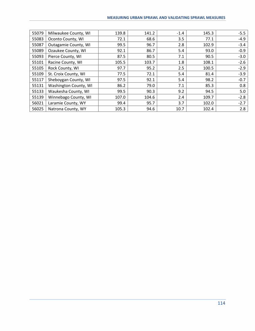
MEASURING URBAN SPRAWL AND VALIDATING SPRAWL MEASURES
114
55079 Milwaukee County, WI 139.8 141.2 -1.4 145.3 -5.5
55083 Oconto County, WI 72.1 68.6 3.5 77.1 -4.9
55087 Outagamie County, WI 99.5 96.7 2.8 102.9 -3.4
55089 Ozaukee County, WI 92.1 86.7 5.4 93.0 -0.9
55093 Pierce County, WI 87.5 80.5 7.1 90.5 -3.0
55101 Racine County, WI 105.5 103.7 1.8 108.1 -2.6
55105 Rock County, WI 97.7 95.2 2.5 100.5 -2.9
55109 St. Croix County, WI 77.5 72.1 5.4 81.4 -3.9
55117 Sheboygan County, WI 97.5 92.1 5.4 98.2 -0.7
55131 Washington County, WI 86.2 79.0 7.1 85.3 0.8
55133 Waukesha County, WI 99.5 90.3 9.2 94.5 5.0
55139 Winnebago County, WI 107.0 104.6 2.4 109.7 -2.8
56021 Laramie County, WY 99.4 95.7 3.7 102.0 -2.7
56025 Natrona County, WY 105.3 94.6 10.7 102.4 2.8
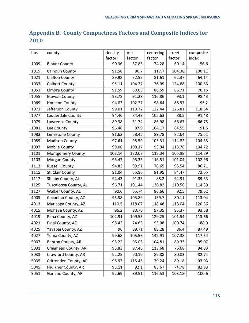
MEASURING URBAN SPRAWL AND VALIDATING SPRAWL MEASURES
115
Appendix B. County Compactness Factors and Composite Indices for
2010
fips county density factor
mix factor
centering factor
street factor
composite index
1009 Blount County 90.36 37.85 74.28 60.14 56.6
1015 Calhoun County 91.58 86.7 117.7 104.38 100.11
1021 Chilton County 89.98 52.55 81.61 62.37 64.14
1033 Colbert County 95.11 104.27 76.99 124.68 100.33
1051 Elmore County 91.59 60.63 86.59 85.71 76.15
1055 Etowah County 93.78 91.28 116.86 93.1 98.43
1069 Houston County 94.83 102.37 98.64 88.97 95.2
1073 Jefferson County 99.01 110.72 122.44 126.81 118.64
1077 Lauderdale County 94.46 84.43 105.63 88.5 91.48
1079 Lawrence County 89.38 51.74 86.98 66.67 66.75
1081 Lee County 96.48 87.9 104.17 84.55 91.5
1083 Limestone County 91.62 58.45 89.78 82.64 75.51
1089 Madison County 97.61 98.59 103.31 114.82 104.53
1097 Mobile County 99.06 108.17 93.94 113.78 104.72
1101 Montgomery County 102.14 120.67 118.34 105.98 114.89
1103 Morgan County 96.47 95.35 116.51 101.04 102.96
1113 Russell County 94.83 90.91 78.65 93.54 86.71
1115 St. Clair County 91.04 55.96 81.95 84.47 72.65
1117 Shelby County, AL 94.43 91.33 88.2 92.91 89.53
1125 Tuscaloosa County, AL 96.71 101.44 136.82 110.56 114.39
1127 Walker County, AL 90.6 65.74 86.66 92.5 79.62
4005 Coconino County, AZ 95.58 105.89 159.7 80.11 113.04
4013 Maricopa County, AZ 110.5 118.07 118.48 118.04 120.56
4015 Mohave County, AZ 96.2 90.76 97.35 95.37 93.58
4019 Pima County, AZ 102.91 109.55 129.25 101.54 113.66
4021 Pinal County, AZ 96.42 74.63 93.08 100.74 88.9
4025 Yavapai County, AZ 96 89.71 88.28 86.4 87.49
4027 Yuma County, AZ 99.68 105.56 142.91 107.38 117.54
5007 Benton County, AR 95.22 95.05 104.81 89.33 95.07
5031 Craighead County, AR 95.83 97.46 113.68 76.68 94.83
5033 Crawford County, AR 92.25 90.19 82.88 80.03 82.74
5035 Crittenden County, AR 96.93 115.43 79.24 89.18 93.93
5045 Faulkner County, AR 95.11 92.1 83.67 74.78 82.83
5051 Garland County, AR 92.69 89.51 116.53 103.18 100.6
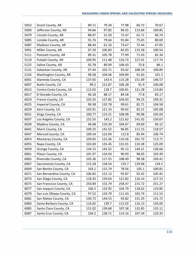
MEASURING URBAN SPRAWL AND VALIDATING SPRAWL MEASURES
116
5053 Grant County, AR 89.11 79.34 77.98 60.72 70.67
5069 Jefferson County, AR 94.66 97.82 96.55 113.66 100.85
5079 Lincoln County, AR 88.97 51.59 72.47 62.71 60.74
5085 Lonoke County, AR 91.76 79.64 91.84 75.65 80.69
5087 Madison County, AR 88.44 61.16 73.67 72.44 67.05
5091 Miller County, AR 97.29 106.83 82.03 115.58 100.54
5111 Poinsett County, AR 89.31 105.78 77.99 71.03 82.34
5119 Pulaski County, AR 100.95 111.48 116.72 127.01 117.74
5125 Saline County, AR 92.78 80.99 106.43 75.8 86.1
5131 Sebastian County, AR 97.44 103.71 93.42 108.24 100.89
5143 Washington County, AR 98.58 104.46 109.89 91.83 101.5
6001 Alameda County, CA 137.65 143.4 115.28 151.09 146.57
6007 Butte County, CA 99.2 121.87 106.28 91.9 106.08
6013 Contra Costa County, CA 112.02 128.7 100.81 121.28 119.84
6017 El Dorado County, CA 96.18 88.17 84.58 77.8 83.17
6019 Fresno County, CA 103.35 127.85 104.03 94.25 109.31
6025 Imperial County, CA 99.38 132.78 99.61 82.71 104.58
6029 Kern County, CA 102.91 121.33 99.62 92.21 105.08
6031 Kings County, CA 100.77 115.21 108.98 90.98 105.04
6037 Los Angeles County, CA 152.55 145.2 121.62 141.02 150.67
6039 Madera County, CA 96.68 110.34 104.67 69.69 94.12
6041 Marin County, CA 109.25 141.52 96.85 111.15 118.57
6047 Merced County, CA 100.54 122.04 112.8 85.94 106.74
6053 Monterey County, CA 109.05 122.36 110.26 101.72 113.71
6055 Napa County, CA 102.69 135.45 131.01 110.28 125.09
6059 Orange County, CA 134.15 142.55 95.13 144.21 136.66
6061 Placer County, CA 101.97 116.93 90.93 98.05 102.49
6065 Riverside County, CA 105.36 117.55 108.49 98.38 109.41
6067 Sacramento County, CA 115.28 128.54 135.7 129.68 134.5
6069 San Benito County, CA 103.1 115.79 78.56 105.1 100.81
6071 San Bernardino County, CA 106.82 122.13 95.87 92.42 105.45
6073 San Diego County, CA 118.35 129.64 121.82 116.14 127.15
6075 San Francisco County, CA 250.84 153.79 258.47 215.72 251.27
6077 San Joaquin County, CA 106.5 132.92 104.79 118.62 119.85
6079 San Luis Obispo County, CA 97.52 124.79 111.43 102.74 111.53
6081 San Mateo County, CA 130.72 144.53 93.82 131.35 131.72
6083 Santa Barbara County, CA 116.62 139.7 112.02 116.13 126.69
6085 Santa Clara County, CA 131.02 139.68 107.58 132.85 135.11
6087 Santa Cruz County, CA 104.2 138.71 114.16 107.34 120.35
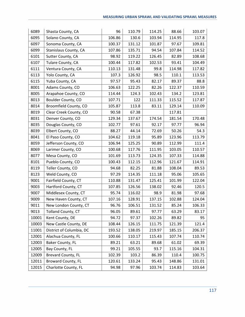
MEASURING URBAN SPRAWL AND VALIDATING SPRAWL MEASURES
117
6089 Shasta County, CA 96 110.79 114.25 88.66 103.07
6095 Solano County, CA 106.86 130.6 103.94 114.95 117.8
6097 Sonoma County, CA 100.37 131.12 101.87 97.67 109.81
6099 Stanislaus County, CA 107.86 135.71 94.54 107.84 114.52
6101 Sutter County, CA 98.92 119.22 126.45 82.89 108.68
6107 Tulare County, CA 100.44 117.82 102.53 93.41 104.49
6111 Ventura County, CA 110.13 131.48 99.8 114.98 117.82
6113 Yolo County, CA 107.3 126.92 98.5 110.1 113.53
6115 Yuba County, CA 97.57 95.43 82.17 89.37 88.8
8001 Adams County, CO 106.63 122.25 82.26 122.37 110.59
8005 Arapahoe County, CO 114.44 124.3 102.43 134.2 123.81
8013 Boulder County, CO 107.71 122 111.33 115.52 117.87
8014 Broomfield County, CO 105.87 113.8 83.11 129.14 110.09
8019 Clear Creek County, CO 90.58 67.38 117.81
8031 Denver County, CO 129.34 137.67 174.54 181.54 170.48
8035 Douglas County, CO 102.77 97.61 92.17 97.77 96.94
8039 Elbert County, CO 88.27 44.14 72.69 50.26 54.3
8041 El Paso County, CO 104.62 119.18 95.89 123.96 113.79
8059 Jefferson County, CO 106.94 125.25 90.89 112.99 111.4
8069 Larimer County, CO 100.68 117.76 111.95 103.05 110.57
8077 Mesa County, CO 101.69 113.73 124.35 107.33 114.88
8101 Pueblo County, CO 100.43 112.15 112.96 121.67 114.91
8119 Teller County, CO 94.68 82.25 81.88 108.04 89.53
8123 Weld County, CO 97.29 114.35 111.18 95.06 105.65
9001 Fairfield County, CT 110.88 131.47 125.41 101.99 122.04
9003 Hartford County, CT 107.85 126.56 138.02 92.46 120.5
9007 Middlesex County, CT 95.74 116.02 98.9 81.98 97.68
9009 New Haven County, CT 107.16 128.91 137.15 102.88 124.04
9011 New London County, CT 96.76 106.51 131.52 85.24 106.33
9013 Tolland County, CT 96.05 89.61 97.77 63.29 83.17
10001 Kent County, DE 94.72 97.37 102.26 89.82 95
10003 New Castle County, DE 108.44 126.15 111.75 121.39 121.4
11001 District of Columbia, DC 193.52 138.05 219.97 185.15 206.37
12001 Alachua County, FL 100.66 110.17 115.43 107.74 110.74
12003 Baker County, FL 89.21 63.21 89.68 61.02 69.39
12005 Bay County, FL 99.21 105.55 93.7 115.16 104.31
12009 Brevard County, FL 102.39 103.2 86.39 110.4 100.75
12011 Broward County, FL 120.61 133.24 95.43 148.86 131.01
12015 Charlotte County, FL 94.98 97.96 103.74 114.83 103.64
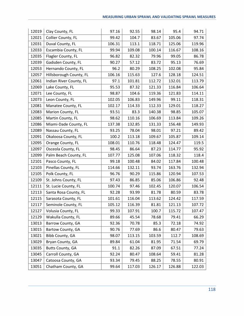
MEASURING URBAN SPRAWL AND VALIDATING SPRAWL MEASURES
118
12019 Clay County, FL 97.16 92.55 98.14 95.4 94.71
12021 Collier County, FL 99.42 104.7 83.67 105.06 97.74
12031 Duval County, FL 106.31 113.1 118.71 125.06 119.96
12033 Escambia County, FL 99.94 109.08 100.14 116.67 108.16
12035 Flagler County, FL 96.82 82.32 79.96 99.05 86.78
12039 Gadsden County, FL 90.27 57.12 83.72 95.13 76.69
12053 Hernando County, FL 96.2 80.29 108.25 102.08 95.84
12057 Hillsborough County, FL 106.16 115.63 127.6 128.18 124.51
12061 Indian River County, FL 97.1 101.81 112.72 132.01 113.79
12069 Lake County, FL 95.53 87.32 121.33 116.84 106.64
12071 Lee County, FL 98.87 104.6 119.36 121.83 114.11
12073 Leon County, FL 102.05 106.83 149.96 99.11 118.31
12081 Manatee County, FL 102.17 114.33 112.33 129.01 118.27
12083 Marion County, FL 93.51 83.3 140.38 98.85 105.07
12085 Martin County, FL 98.62 110.16 106.69 113.84 109.26
12086 Miami-Dade County, FL 137.38 132.85 131.33 156.48 149.93
12089 Nassau County, FL 93.25 78.04 98.01 97.21 89.42
12091 Okaloosa County, FL 100.2 113.18 109.67 105.87 109.14
12095 Orange County, FL 108.01 110.76 118.48 124.47 119.5
12097 Osceola County, FL 98.45 86.64 87.23 114.77 95.92
12099 Palm Beach County, FL 107.77 125.08 107.06 118.32 118.4
12101 Pasco County, FL 99.18 100.48 84.02 117.84 100.48
12103 Pinellas County, FL 114.66 132.11 93.74 163.76 132.94
12105 Polk County, FL 96.76 90.29 115.86 120.94 107.53
12109 St. Johns County, FL 97.43 86.85 85.06 106.86 92.48
12111 St. Lucie County, FL 100.74 97.46 102.45 120.07 106.54
12113 Santa Rosa County, FL 92.28 93.99 81.78 80.59 83.78
12115 Sarasota County, FL 101.61 116.04 113.62 124.42 117.59
12117 Seminole County, FL 105.12 116.39 81.81 121.13 107.72
12127 Volusia County, FL 99.33 107.91 100.7 115.72 107.47
12129 Wakulla County, FL 89.66 45.54 78.68 79.41 66.29
13013 Barrow County, GA 92.36 70.78 85.3 72.18 74.92
13015 Bartow County, GA 90.76 77.69 86.6 80.47 79.63
13021 Bibb County, GA 98.07 113.15 103.59 112.7 108.69
13029 Bryan County, GA 89.84 61.04 81.95 71.54 69.79
13035 Butts County, GA 91.1 82.26 87.09 67.51 77.24
13045 Carroll County, GA 92.24 80.47 108.64 59.41 81.28
13047 Catoosa County, GA 93.34 79.45 88.25 78.55 80.91
13051 Chatham County, GA 99.64 117.03 126.17 126.88 122.03
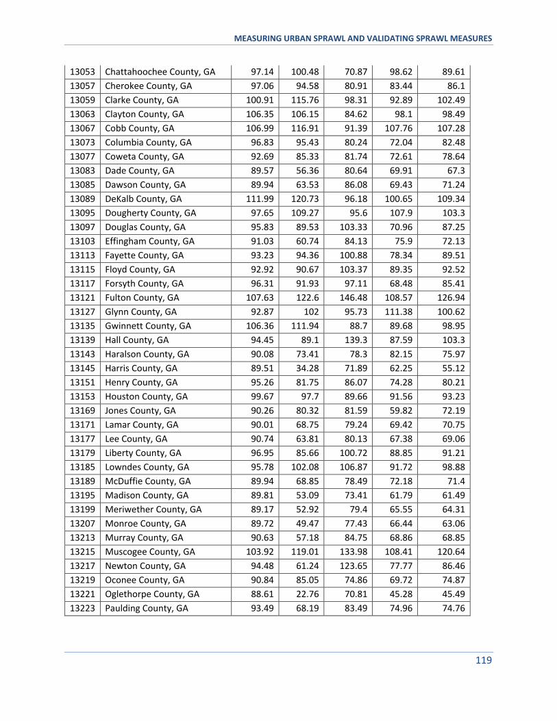
MEASURING URBAN SPRAWL AND VALIDATING SPRAWL MEASURES
119
13053 Chattahoochee County, GA 97.14 100.48 70.87 98.62 89.61
13057 Cherokee County, GA 97.06 94.58 80.91 83.44 86.1
13059 Clarke County, GA 100.91 115.76 98.31 92.89 102.49
13063 Clayton County, GA 106.35 106.15 84.62 98.1 98.49
13067 Cobb County, GA 106.99 116.91 91.39 107.76 107.28
13073 Columbia County, GA 96.83 95.43 80.24 72.04 82.48
13077 Coweta County, GA 92.69 85.33 81.74 72.61 78.64
13083 Dade County, GA 89.57 56.36 80.64 69.91 67.3
13085 Dawson County, GA 89.94 63.53 86.08 69.43 71.24
13089 DeKalb County, GA 111.99 120.73 96.18 100.65 109.34
13095 Dougherty County, GA 97.65 109.27 95.6 107.9 103.3
13097 Douglas County, GA 95.83 89.53 103.33 70.96 87.25
13103 Effingham County, GA 91.03 60.74 84.13 75.9 72.13
13113 Fayette County, GA 93.23 94.36 100.88 78.34 89.51
13115 Floyd County, GA 92.92 90.67 103.37 89.35 92.52
13117 Forsyth County, GA 96.31 91.93 97.11 68.48 85.41
13121 Fulton County, GA 107.63 122.6 146.48 108.57 126.94
13127 Glynn County, GA 92.87 102 95.73 111.38 100.62
13135 Gwinnett County, GA 106.36 111.94 88.7 89.68 98.95
13139 Hall County, GA 94.45 89.1 139.3 87.59 103.3
13143 Haralson County, GA 90.08 73.41 78.3 82.15 75.97
13145 Harris County, GA 89.51 34.28 71.89 62.25 55.12
13151 Henry County, GA 95.26 81.75 86.07 74.28 80.21
13153 Houston County, GA 99.67 97.7 89.66 91.56 93.23
13169 Jones County, GA 90.26 80.32 81.59 59.82 72.19
13171 Lamar County, GA 90.01 68.75 79.24 69.42 70.75
13177 Lee County, GA 90.74 63.81 80.13 67.38 69.06
13179 Liberty County, GA 96.95 85.66 100.72 88.85 91.21
13185 Lowndes County, GA 95.78 102.08 106.87 91.72 98.88
13189 McDuffie County, GA 89.94 68.85 78.49 72.18 71.4
13195 Madison County, GA 89.81 53.09 73.41 61.79 61.49
13199 Meriwether County, GA 89.17 52.92 79.4 65.55 64.31
13207 Monroe County, GA 89.72 49.47 77.43 66.44 63.06
13213 Murray County, GA 90.63 57.18 84.75 68.86 68.85
13215 Muscogee County, GA 103.92 119.01 133.98 108.41 120.64
13217 Newton County, GA 94.48 61.24 123.65 77.77 86.46
13219 Oconee County, GA 90.84 85.05 74.86 69.72 74.87
13221 Oglethorpe County, GA 88.61 22.76 70.81 45.28 45.49
13223 Paulding County, GA 93.49 68.19 83.49 74.96 74.76
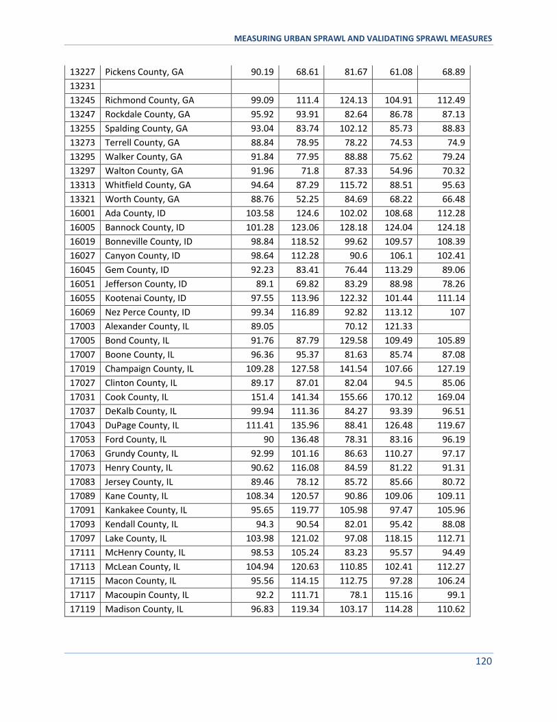
MEASURING URBAN SPRAWL AND VALIDATING SPRAWL MEASURES
120
13227 Pickens County, GA 90.19 68.61 81.67 61.08 68.89
13231
13245 Richmond County, GA 99.09 111.4 124.13 104.91 112.49
13247 Rockdale County, GA 95.92 93.91 82.64 86.78 87.13
13255 Spalding County, GA 93.04 83.74 102.12 85.73 88.83
13273 Terrell County, GA 88.84 78.95 78.22 74.53 74.9
13295 Walker County, GA 91.84 77.95 88.88 75.62 79.24
13297 Walton County, GA 91.96 71.8 87.33 54.96 70.32
13313 Whitfield County, GA 94.64 87.29 115.72 88.51 95.63
13321 Worth County, GA 88.76 52.25 84.69 68.22 66.48
16001 Ada County, ID 103.58 124.6 102.02 108.68 112.28
16005 Bannock County, ID 101.28 123.06 128.18 124.04 124.18
16019 Bonneville County, ID 98.84 118.52 99.62 109.57 108.39
16027 Canyon County, ID 98.64 112.28 90.6 106.1 102.41
16045 Gem County, ID 92.23 83.41 76.44 113.29 89.06
16051 Jefferson County, ID 89.1 69.82 83.29 88.98 78.26
16055 Kootenai County, ID 97.55 113.96 122.32 101.44 111.14
16069 Nez Perce County, ID 99.34 116.89 92.82 113.12 107
17003 Alexander County, IL 89.05 70.12 121.33
17005 Bond County, IL 91.76 87.79 129.58 109.49 105.89
17007 Boone County, IL 96.36 95.37 81.63 85.74 87.08
17019 Champaign County, IL 109.28 127.58 141.54 107.66 127.19
17027 Clinton County, IL 89.17 87.01 82.04 94.5 85.06
17031 Cook County, IL 151.4 141.34 155.66 170.12 169.04
17037 DeKalb County, IL 99.94 111.36 84.27 93.39 96.51
17043 DuPage County, IL 111.41 135.96 88.41 126.48 119.67
17053 Ford County, IL 90 136.48 78.31 83.16 96.19
17063 Grundy County, IL 92.99 101.16 86.63 110.27 97.17
17073 Henry County, IL 90.62 116.08 84.59 81.22 91.31
17083 Jersey County, IL 89.46 78.12 85.72 85.66 80.72
17089 Kane County, IL 108.34 120.57 90.86 109.06 109.11
17091 Kankakee County, IL 95.65 119.77 105.98 97.47 105.96
17093 Kendall County, IL 94.3 90.54 82.01 95.42 88.08
17097 Lake County, IL 103.98 121.02 97.08 118.15 112.71
17111 McHenry County, IL 98.53 105.24 83.23 95.57 94.49
17113 McLean County, IL 104.94 120.63 110.85 102.41 112.27
17115 Macon County, IL 95.56 114.15 112.75 97.28 106.24
17117 Macoupin County, IL 92.2 111.71 78.1 115.16 99.1
17119 Madison County, IL 96.83 119.34 103.17 114.28 110.62
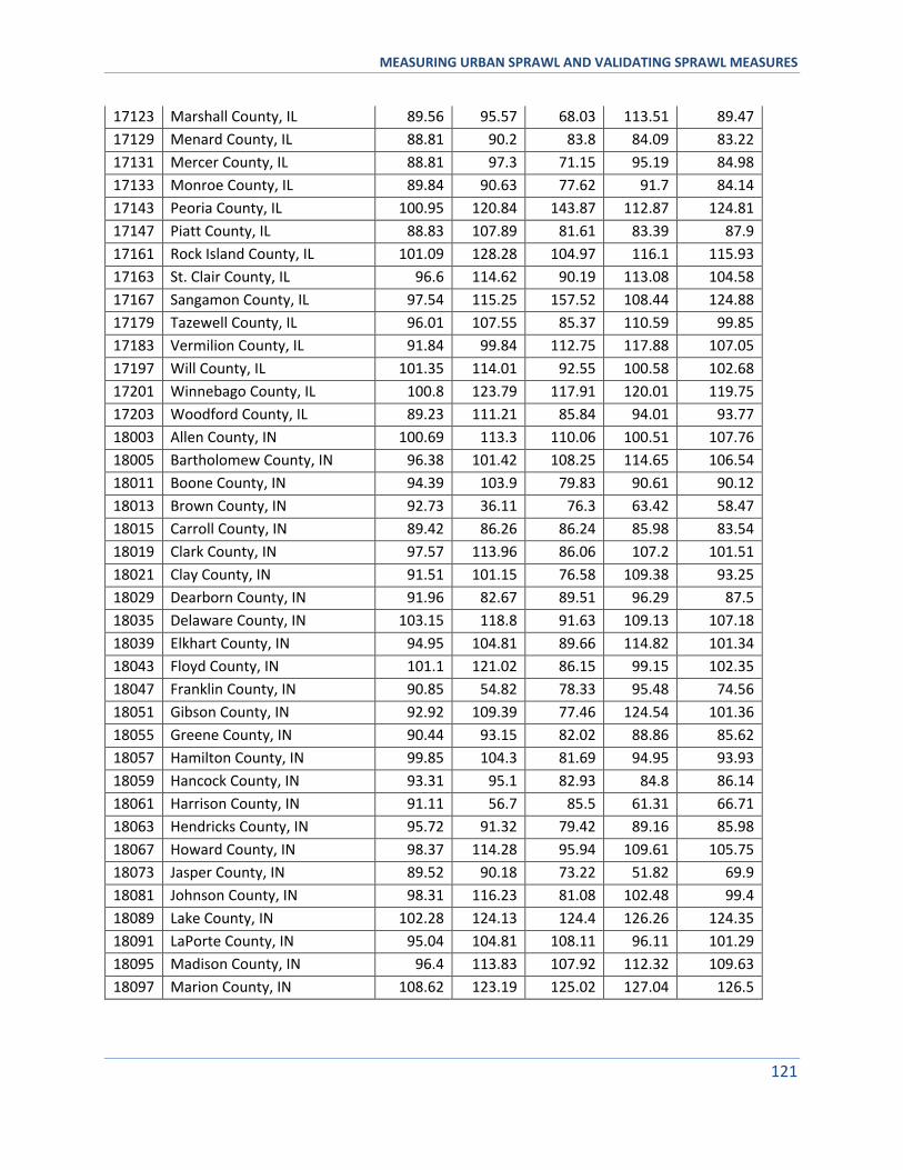
MEASURING URBAN SPRAWL AND VALIDATING SPRAWL MEASURES
121
17123 Marshall County, IL 89.56 95.57 68.03 113.51 89.47
17129 Menard County, IL 88.81 90.2 83.8 84.09 83.22
17131 Mercer County, IL 88.81 97.3 71.15 95.19 84.98
17133 Monroe County, IL 89.84 90.63 77.62 91.7 84.14
17143 Peoria County, IL 100.95 120.84 143.87 112.87 124.81
17147 Piatt County, IL 88.83 107.89 81.61 83.39 87.9
17161 Rock Island County, IL 101.09 128.28 104.97 116.1 115.93
17163 St. Clair County, IL 96.6 114.62 90.19 113.08 104.58
17167 Sangamon County, IL 97.54 115.25 157.52 108.44 124.88
17179 Tazewell County, IL 96.01 107.55 85.37 110.59 99.85
17183 Vermilion County, IL 91.84 99.84 112.75 117.88 107.05
17197 Will County, IL 101.35 114.01 92.55 100.58 102.68
17201 Winnebago County, IL 100.8 123.79 117.91 120.01 119.75
17203 Woodford County, IL 89.23 111.21 85.84 94.01 93.77
18003 Allen County, IN 100.69 113.3 110.06 100.51 107.76
18005 Bartholomew County, IN 96.38 101.42 108.25 114.65 106.54
18011 Boone County, IN 94.39 103.9 79.83 90.61 90.12
18013 Brown County, IN 92.73 36.11 76.3 63.42 58.47
18015 Carroll County, IN 89.42 86.26 86.24 85.98 83.54
18019 Clark County, IN 97.57 113.96 86.06 107.2 101.51
18021 Clay County, IN 91.51 101.15 76.58 109.38 93.25
18029 Dearborn County, IN 91.96 82.67 89.51 96.29 87.5
18035 Delaware County, IN 103.15 118.8 91.63 109.13 107.18
18039 Elkhart County, IN 94.95 104.81 89.66 114.82 101.34
18043 Floyd County, IN 101.1 121.02 86.15 99.15 102.35
18047 Franklin County, IN 90.85 54.82 78.33 95.48 74.56
18051 Gibson County, IN 92.92 109.39 77.46 124.54 101.36
18055 Greene County, IN 90.44 93.15 82.02 88.86 85.62
18057 Hamilton County, IN 99.85 104.3 81.69 94.95 93.93
18059 Hancock County, IN 93.31 95.1 82.93 84.8 86.14
18061 Harrison County, IN 91.11 56.7 85.5 61.31 66.71
18063 Hendricks County, IN 95.72 91.32 79.42 89.16 85.98
18067 Howard County, IN 98.37 114.28 95.94 109.61 105.75
18073 Jasper County, IN 89.52 90.18 73.22 51.82 69.9
18081 Johnson County, IN 98.31 116.23 81.08 102.48 99.4
18089 Lake County, IN 102.28 124.13 124.4 126.26 124.35
18091 LaPorte County, IN 95.04 104.81 108.11 96.11 101.29
18095 Madison County, IN 96.4 113.83 107.92 112.32 109.63
18097 Marion County, IN 108.62 123.19 125.02 127.04 126.5
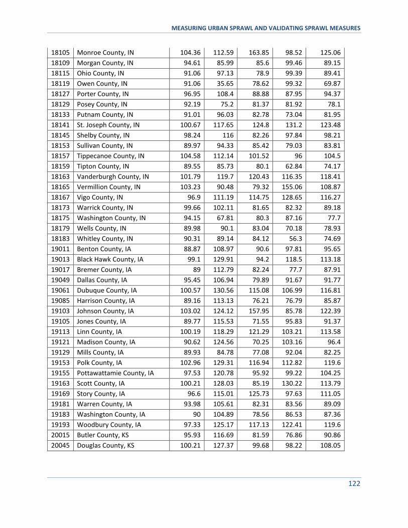
MEASURING URBAN SPRAWL AND VALIDATING SPRAWL MEASURES
122
18105 Monroe County, IN 104.36 112.59 163.85 98.52 125.06
18109 Morgan County, IN 94.61 85.99 85.6 99.46 89.15
18115 Ohio County, IN 91.06 97.13 78.9 99.39 89.41
18119 Owen County, IN 91.06 35.65 78.62 99.32 69.87
18127 Porter County, IN 96.95 108.4 88.88 87.95 94.37
18129 Posey County, IN 92.19 75.2 81.37 81.92 78.1
18133 Putnam County, IN 91.01 96.03 82.78 73.04 81.95
18141 St. Joseph County, IN 100.67 117.65 124.8 131.2 123.48
18145 Shelby County, IN 98.24 116 82.26 97.84 98.21
18153 Sullivan County, IN 89.97 94.33 85.42 79.03 83.81
18157 Tippecanoe County, IN 104.58 112.14 101.52 96 104.5
18159 Tipton County, IN 89.55 85.73 80.1 62.84 74.17
18163 Vanderburgh County, IN 101.79 119.7 120.43 116.35 118.41
18165 Vermillion County, IN 103.23 90.48 79.32 155.06 108.87
18167 Vigo County, IN 96.9 111.19 114.75 128.65 116.27
18173 Warrick County, IN 99.66 102.11 81.65 82.32 89.18
18175 Washington County, IN 94.15 67.81 80.3 87.16 77.7
18179 Wells County, IN 89.98 90.1 83.04 70.18 78.93
18183 Whitley County, IN 90.31 89.14 84.12 56.3 74.69
19011 Benton County, IA 88.87 108.97 90.6 97.81 95.65
19013 Black Hawk County, IA 99.1 129.91 94.2 118.5 113.18
19017 Bremer County, IA 89 112.79 82.24 77.7 87.91
19049 Dallas County, IA 95.45 106.94 79.89 91.67 91.77
19061 Dubuque County, IA 100.57 130.56 115.08 106.99 116.81
19085 Harrison County, IA 89.16 113.13 76.21 76.79 85.87
19103 Johnson County, IA 103.02 124.12 157.95 85.78 122.39
19105 Jones County, IA 89.77 115.53 71.55 95.83 91.37
19113 Linn County, IA 100.19 118.29 121.29 103.21 113.58
19121 Madison County, IA 90.62 124.56 70.25 103.16 96.4
19129 Mills County, IA 89.93 84.78 77.08 92.04 82.25
19153 Polk County, IA 102.96 129.31 116.94 112.82 119.6
19155 Pottawattamie County, IA 97.53 120.78 95.92 99.22 104.25
19163 Scott County, IA 100.21 128.03 85.19 130.22 113.79
19169 Story County, IA 96.6 115.01 125.73 97.63 111.05
19181 Warren County, IA 93.98 105.61 82.31 83.56 89.09
19183 Washington County, IA 90 104.89 78.56 86.53 87.36
19193 Woodbury County, IA 97.33 125.17 117.13 122.41 119.6
20015 Butler County, KS 95.93 116.69 81.59 76.86 90.86
20045 Douglas County, KS 100.21 127.37 99.68 98.22 108.05
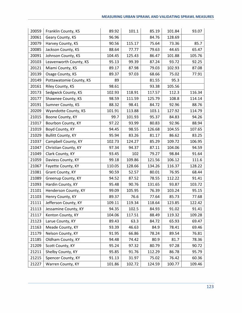
MEASURING URBAN SPRAWL AND VALIDATING SPRAWL MEASURES
123
20059 Franklin County, KS 89.92 101.1 85.19 101.84 93.07
20061 Geary County, KS 96.96 84.76 128.69
20079 Harvey County, KS 90.56 115.17 75.64 73.36 85.7
20085 Jackson County, KS 88.64 77.77 79.63 44.65 65.47
20091 Johnson County, KS 104.45 125.43 86.47 101.88 105.76
20103 Leavenworth County, KS 95.13 99.39 87.24 93.72 92.25
20121 Miami County, KS 89.17 87.98 79.03 102.93 87.08
20139 Osage County, KS 89.37 97.03 68.66 75.02 77.91
20149 Pottawatomie County, KS 89 81.55 95.3
20161 Riley County, KS 98.61 93.38 105.56
20173 Sedgwick County, KS 102.93 118.91 117.57 112.3 116.34
20177 Shawnee County, KS 98.59 111.59 125.79 108.8 114.14
20191 Sumner County, KS 88.32 98.41 84.72 92.96 88.76
20209 Wyandotte County, KS 101.91 113.88 103.1 127.92 114.79
21015 Boone County, KY 99.7 101.93 95.37 84.83 94.26
21017 Bourbon County, KY 97.22 93.99 80.83 92.96 88.94
21019 Boyd County, KY 94.45 98.55 126.68 104.55 107.65
21029 Bullitt County, KY 95.94 83.26 81.17 86.62 83.25
21037 Campbell County, KY 102.73 124.27 85.29 109.72 106.95
21047 Christian County, KY 97.34 94.37 87.11 104.06 94.59
21049 Clark County, KY 93.45 102 79.27 98.84 91.64
21059 Daviess County, KY 99.18 109.86 121.56 106.12 111.6
21067 Fayette County, KY 110.05 128.66 134.26 116.37 128.22
21081 Grant County, KY 90.59 52.57 80.01 76.95 68.44
21089 Greenup County, KY 94.52 87.52 78.55 112.22 91.41
21093 Hardin County, KY 95.48 90.76 131.65 93.87 103.72
21101 Henderson County, KY 99.09 105.95 76.39 103.24 95.15
21103 Henry County, KY 89.37 76.6 77.64 85.73 77.68
21111 Jefferson County, KY 109.11 119.34 118.64 123.85 122.42
21113 Jessamine County, KY 94.35 102.5 84.93 91.02 91.41
21117 Kenton County, KY 104.06 117.51 88.49 119.32 109.28
21123 Larue County, KY 89.43 63.3 84.72 65.93 69.47
21163 Meade County, KY 93.39 46.63 84.9 78.41 69.46
21179 Nelson County, KY 91.95 66.86 78.24 89.54 76.81
21185 Oldham County, KY 94.48 74.42 80.9 81.7 78.36
21209 Scott County, KY 95.24 97.32 80.79 97.28 90.72
21211 Shelby County, KY 95.85 91.76 112.29 86.78 95.79
21215 Spencer County, KY 91.13 31.97 75.02 76.42 60.36
21227 Warren County, KY 101.86 102.72 124.59 100.77 109.46
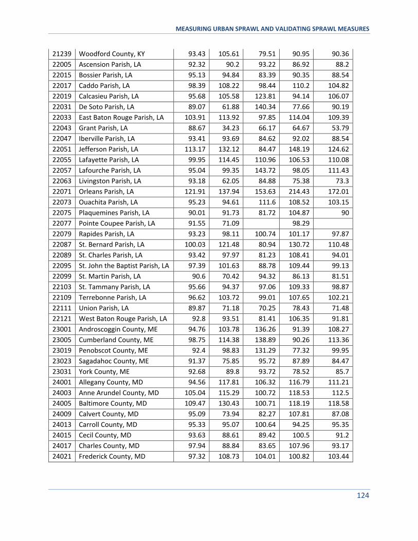
MEASURING URBAN SPRAWL AND VALIDATING SPRAWL MEASURES
124
21239 Woodford County, KY 93.43 105.61 79.51 90.95 90.36
22005 Ascension Parish, LA 92.32 90.2 93.22 86.92 88.2
22015 Bossier Parish, LA 95.13 94.84 83.39 90.35 88.54
22017 Caddo Parish, LA 98.39 108.22 98.44 110.2 104.82
22019 Calcasieu Parish, LA 95.68 105.58 123.81 94.14 106.07
22031 De Soto Parish, LA 89.07 61.88 140.34 77.66 90.19
22033 East Baton Rouge Parish, LA 103.91 113.92 97.85 114.04 109.39
22043 Grant Parish, LA 88.67 34.23 66.17 64.67 53.79
22047 Iberville Parish, LA 93.41 93.69 84.62 92.02 88.54
22051 Jefferson Parish, LA 113.17 132.12 84.47 148.19 124.62
22055 Lafayette Parish, LA 99.95 114.45 110.96 106.53 110.08
22057 Lafourche Parish, LA 95.04 99.35 143.72 98.05 111.43
22063 Livingston Parish, LA 93.18 62.05 84.88 75.38 73.3
22071 Orleans Parish, LA 121.91 137.94 153.63 214.43 172.01
22073 Ouachita Parish, LA 95.23 94.61 111.6 108.52 103.15
22075 Plaquemines Parish, LA 90.01 91.73 81.72 104.87 90
22077 Pointe Coupee Parish, LA 91.55 71.09 98.29
22079 Rapides Parish, LA 93.23 98.11 100.74 101.17 97.87
22087 St. Bernard Parish, LA 100.03 121.48 80.94 130.72 110.48
22089 St. Charles Parish, LA 93.42 97.97 81.23 108.41 94.01
22095 St. John the Baptist Parish, LA 97.39 101.63 88.78 109.44 99.13
22099 St. Martin Parish, LA 90.6 70.42 94.32 86.13 81.51
22103 St. Tammany Parish, LA 95.66 94.37 97.06 109.33 98.87
22109 Terrebonne Parish, LA 96.62 103.72 99.01 107.65 102.21
22111 Union Parish, LA 89.87 71.18 70.25 78.43 71.48
22121 West Baton Rouge Parish, LA 92.8 93.51 81.41 106.35 91.81
23001 Androscoggin County, ME 94.76 103.78 136.26 91.39 108.27
23005 Cumberland County, ME 98.75 114.38 138.89 90.26 113.36
23019 Penobscot County, ME 92.4 98.83 131.29 77.32 99.95
23023 Sagadahoc County, ME 91.37 75.85 95.72 87.89 84.47
23031 York County, ME 92.68 89.8 93.72 78.52 85.7
24001 Allegany County, MD 94.56 117.81 106.32 116.79 111.21
24003 Anne Arundel County, MD 105.04 115.29 100.72 118.53 112.5
24005 Baltimore County, MD 109.47 130.43 100.71 118.19 118.58
24009 Calvert County, MD 95.09 73.94 82.27 107.81 87.08
24013 Carroll County, MD 95.33 95.07 100.64 94.25 95.35
24015 Cecil County, MD 93.63 88.61 89.42 100.5 91.2
24017 Charles County, MD 97.94 88.84 83.65 107.96 93.17
24021 Frederick County, MD 97.32 108.73 104.01 100.82 103.44
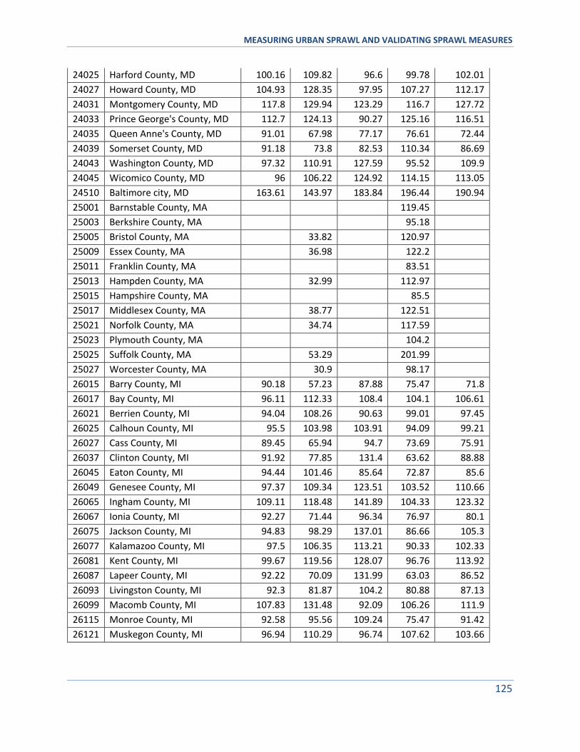
MEASURING URBAN SPRAWL AND VALIDATING SPRAWL MEASURES
125
24025 Harford County, MD 100.16 109.82 96.6 99.78 102.01
24027 Howard County, MD 104.93 128.35 97.95 107.27 112.17
24031 Montgomery County, MD 117.8 129.94 123.29 116.7 127.72
24033 Prince George's County, MD 112.7 124.13 90.27 125.16 116.51
24035 Queen Anne's County, MD 91.01 67.98 77.17 76.61 72.44
24039 Somerset County, MD 91.18 73.8 82.53 110.34 86.69
24043 Washington County, MD 97.32 110.91 127.59 95.52 109.9
24045 Wicomico County, MD 96 106.22 124.92 114.15 113.05
24510 Baltimore city, MD 163.61 143.97 183.84 196.44 190.94
25001 Barnstable County, MA 119.45
25003 Berkshire County, MA 95.18
25005 Bristol County, MA 33.82 120.97
25009 Essex County, MA 36.98 122.2
25011 Franklin County, MA 83.51
25013 Hampden County, MA 32.99 112.97
25015 Hampshire County, MA 85.5
25017 Middlesex County, MA 38.77 122.51
25021 Norfolk County, MA 34.74 117.59
25023 Plymouth County, MA 104.2
25025 Suffolk County, MA 53.29 201.99
25027 Worcester County, MA 30.9 98.17
26015 Barry County, MI 90.18 57.23 87.88 75.47 71.8
26017 Bay County, MI 96.11 112.33 108.4 104.1 106.61
26021 Berrien County, MI 94.04 108.26 90.63 99.01 97.45
26025 Calhoun County, MI 95.5 103.98 103.91 94.09 99.21
26027 Cass County, MI 89.45 65.94 94.7 73.69 75.91
26037 Clinton County, MI 91.92 77.85 131.4 63.62 88.88
26045 Eaton County, MI 94.44 101.46 85.64 72.87 85.6
26049 Genesee County, MI 97.37 109.34 123.51 103.52 110.66
26065 Ingham County, MI 109.11 118.48 141.89 104.33 123.32
26067 Ionia County, MI 92.27 71.44 96.34 76.97 80.1
26075 Jackson County, MI 94.83 98.29 137.01 86.66 105.3
26077 Kalamazoo County, MI 97.5 106.35 113.21 90.33 102.33
26081 Kent County, MI 99.67 119.56 128.07 96.76 113.92
26087 Lapeer County, MI 92.22 70.09 131.99 63.03 86.52
26093 Livingston County, MI 92.3 81.87 104.2 80.88 87.13
26099 Macomb County, MI 107.83 131.48 92.09 106.26 111.9
26115 Monroe County, MI 92.58 95.56 109.24 75.47 91.42
26121 Muskegon County, MI 96.94 110.29 96.74 107.62 103.66
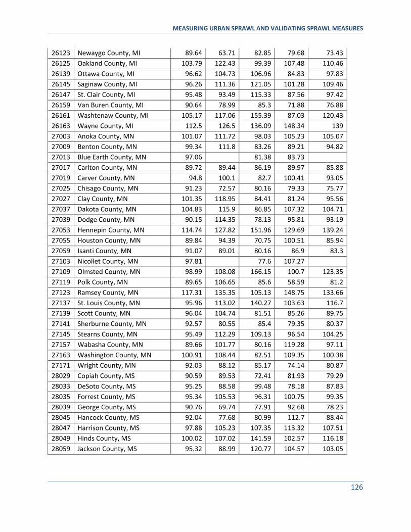
MEASURING URBAN SPRAWL AND VALIDATING SPRAWL MEASURES
126
26123 Newaygo County, MI 89.64 63.71 82.85 79.68 73.43
26125 Oakland County, MI 103.79 122.43 99.39 107.48 110.46
26139 Ottawa County, MI 96.62 104.73 106.96 84.83 97.83
26145 Saginaw County, MI 96.26 111.36 121.05 101.28 109.46
26147 St. Clair County, MI 95.48 93.49 115.33 87.56 97.42
26159 Van Buren County, MI 90.64 78.99 85.3 71.88 76.88
26161 Washtenaw County, MI 105.17 117.06 155.39 87.03 120.43
26163 Wayne County, MI 112.5 126.5 136.09 148.34 139
27003 Anoka County, MN 101.07 111.72 98.03 105.23 105.07
27009 Benton County, MN 99.34 111.8 83.26 89.21 94.82
27013 Blue Earth County, MN 97.06 81.38 83.73
27017 Carlton County, MN 89.72 89.44 86.19 89.97 85.88
27019 Carver County, MN 94.8 100.1 82.7 100.41 93.05
27025 Chisago County, MN 91.23 72.57 80.16 79.33 75.77
27027 Clay County, MN 101.35 118.95 84.41 81.24 95.56
27037 Dakota County, MN 104.83 115.9 86.85 107.32 104.71
27039 Dodge County, MN 90.15 114.35 78.13 95.81 93.19
27053 Hennepin County, MN 114.74 127.82 151.96 129.69 139.24
27055 Houston County, MN 89.84 94.39 70.75 100.51 85.94
27059 Isanti County, MN 91.07 89.01 80.16 86.9 83.3
27103 Nicollet County, MN 97.81 77.6 107.27
27109 Olmsted County, MN 98.99 108.08 166.15 100.7 123.35
27119 Polk County, MN 89.65 106.65 85.6 58.59 81.2
27123 Ramsey County, MN 117.31 135.35 105.13 148.75 133.66
27137 St. Louis County, MN 95.96 113.02 140.27 103.63 116.7
27139 Scott County, MN 96.04 104.74 81.51 85.26 89.75
27141 Sherburne County, MN 92.57 80.55 85.4 79.35 80.37
27145 Stearns County, MN 95.49 112.29 109.13 96.54 104.25
27157 Wabasha County, MN 89.66 101.77 80.16 119.28 97.11
27163 Washington County, MN 100.91 108.44 82.51 109.35 100.38
27171 Wright County, MN 92.03 88.12 85.17 74.14 80.87
28029 Copiah County, MS 90.59 89.53 72.41 81.93 79.29
28033 DeSoto County, MS 95.25 88.58 99.48 78.18 87.83
28035 Forrest County, MS 95.34 105.53 96.31 100.75 99.35
28039 George County, MS 90.76 69.74 77.91 92.68 78.23
28045 Hancock County, MS 92.04 77.68 80.99 112.7 88.44
28047 Harrison County, MS 97.88 105.23 107.35 113.32 107.51
28049 Hinds County, MS 100.02 107.02 141.59 102.57 116.18
28059 Jackson County, MS 95.32 88.99 120.77 104.57 103.05
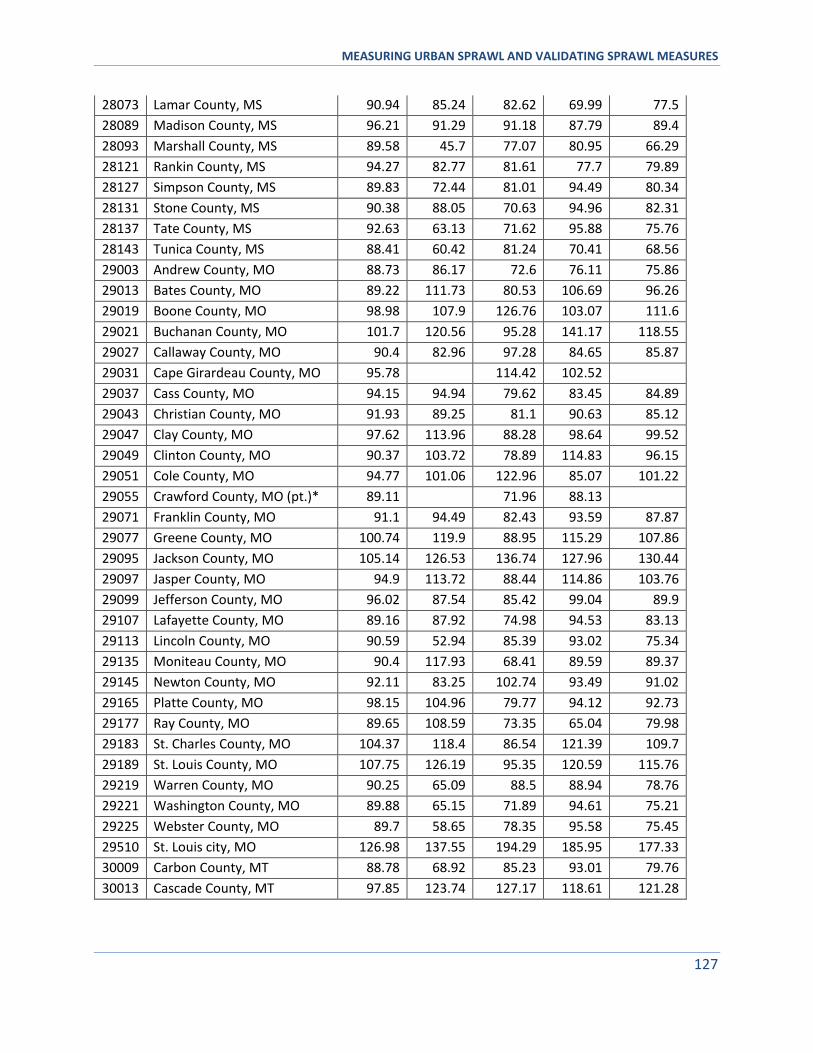
MEASURING URBAN SPRAWL AND VALIDATING SPRAWL MEASURES
127
28073 Lamar County, MS 90.94 85.24 82.62 69.99 77.5
28089 Madison County, MS 96.21 91.29 91.18 87.79 89.4
28093 Marshall County, MS 89.58 45.7 77.07 80.95 66.29
28121 Rankin County, MS 94.27 82.77 81.61 77.7 79.89
28127 Simpson County, MS 89.83 72.44 81.01 94.49 80.34
28131 Stone County, MS 90.38 88.05 70.63 94.96 82.31
28137 Tate County, MS 92.63 63.13 71.62 95.88 75.76
28143 Tunica County, MS 88.41 60.42 81.24 70.41 68.56
29003 Andrew County, MO 88.73 86.17 72.6 76.11 75.86
29013 Bates County, MO 89.22 111.73 80.53 106.69 96.26
29019 Boone County, MO 98.98 107.9 126.76 103.07 111.6
29021 Buchanan County, MO 101.7 120.56 95.28 141.17 118.55
29027 Callaway County, MO 90.4 82.96 97.28 84.65 85.87
29031 Cape Girardeau County, MO 95.78 114.42 102.52
29037 Cass County, MO 94.15 94.94 79.62 83.45 84.89
29043 Christian County, MO 91.93 89.25 81.1 90.63 85.12
29047 Clay County, MO 97.62 113.96 88.28 98.64 99.52
29049 Clinton County, MO 90.37 103.72 78.89 114.83 96.15
29051 Cole County, MO 94.77 101.06 122.96 85.07 101.22
29055 Crawford County, MO (pt.)* 89.11 71.96 88.13
29071 Franklin County, MO 91.1 94.49 82.43 93.59 87.87
29077 Greene County, MO 100.74 119.9 88.95 115.29 107.86
29095 Jackson County, MO 105.14 126.53 136.74 127.96 130.44
29097 Jasper County, MO 94.9 113.72 88.44 114.86 103.76
29099 Jefferson County, MO 96.02 87.54 85.42 99.04 89.9
29107 Lafayette County, MO 89.16 87.92 74.98 94.53 83.13
29113 Lincoln County, MO 90.59 52.94 85.39 93.02 75.34
29135 Moniteau County, MO 90.4 117.93 68.41 89.59 89.37
29145 Newton County, MO 92.11 83.25 102.74 93.49 91.02
29165 Platte County, MO 98.15 104.96 79.77 94.12 92.73
29177 Ray County, MO 89.65 108.59 73.35 65.04 79.98
29183 St. Charles County, MO 104.37 118.4 86.54 121.39 109.7
29189 St. Louis County, MO 107.75 126.19 95.35 120.59 115.76
29219 Warren County, MO 90.25 65.09 88.5 88.94 78.76
29221 Washington County, MO 89.88 65.15 71.89 94.61 75.21
29225 Webster County, MO 89.7 58.65 78.35 95.58 75.45
29510 St. Louis city, MO 126.98 137.55 194.29 185.95 177.33
30009 Carbon County, MT 88.78 68.92 85.23 93.01 79.76
30013 Cascade County, MT 97.85 123.74 127.17 118.61 121.28
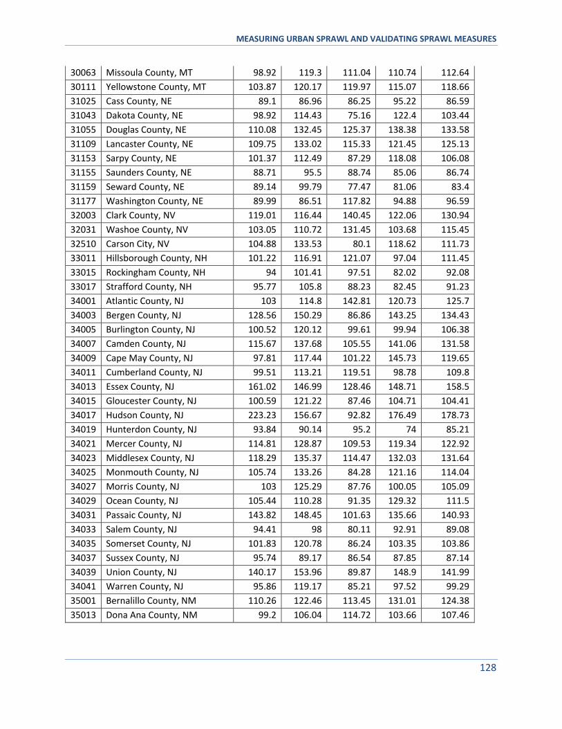
MEASURING URBAN SPRAWL AND VALIDATING SPRAWL MEASURES
128
30063 Missoula County, MT 98.92 119.3 111.04 110.74 112.64
30111 Yellowstone County, MT 103.87 120.17 119.97 115.07 118.66
31025 Cass County, NE 89.1 86.96 86.25 95.22 86.59
31043 Dakota County, NE 98.92 114.43 75.16 122.4 103.44
31055 Douglas County, NE 110.08 132.45 125.37 138.38 133.58
31109 Lancaster County, NE 109.75 133.02 115.33 121.45 125.13
31153 Sarpy County, NE 101.37 112.49 87.29 118.08 106.08
31155 Saunders County, NE 88.71 95.5 88.74 85.06 86.74
31159 Seward County, NE 89.14 99.79 77.47 81.06 83.4
31177 Washington County, NE 89.99 86.51 117.82 94.88 96.59
32003 Clark County, NV 119.01 116.44 140.45 122.06 130.94
32031 Washoe County, NV 103.05 110.72 131.45 103.68 115.45
32510 Carson City, NV 104.88 133.53 80.1 118.62 111.73
33011 Hillsborough County, NH 101.22 116.91 121.07 97.04 111.45
33015 Rockingham County, NH 94 101.41 97.51 82.02 92.08
33017 Strafford County, NH 95.77 105.8 88.23 82.45 91.23
34001 Atlantic County, NJ 103 114.8 142.81 120.73 125.7
34003 Bergen County, NJ 128.56 150.29 86.86 143.25 134.43
34005 Burlington County, NJ 100.52 120.12 99.61 99.94 106.38
34007 Camden County, NJ 115.67 137.68 105.55 141.06 131.58
34009 Cape May County, NJ 97.81 117.44 101.22 145.73 119.65
34011 Cumberland County, NJ 99.51 113.21 119.51 98.78 109.8
34013 Essex County, NJ 161.02 146.99 128.46 148.71 158.5
34015 Gloucester County, NJ 100.59 121.22 87.46 104.71 104.41
34017 Hudson County, NJ 223.23 156.67 92.82 176.49 178.73
34019 Hunterdon County, NJ 93.84 90.14 95.2 74 85.21
34021 Mercer County, NJ 114.81 128.87 109.53 119.34 122.92
34023 Middlesex County, NJ 118.29 135.37 114.47 132.03 131.64
34025 Monmouth County, NJ 105.74 133.26 84.28 121.16 114.04
34027 Morris County, NJ 103 125.29 87.76 100.05 105.09
34029 Ocean County, NJ 105.44 110.28 91.35 129.32 111.5
34031 Passaic County, NJ 143.82 148.45 101.63 135.66 140.93
34033 Salem County, NJ 94.41 98 80.11 92.91 89.08
34035 Somerset County, NJ 101.83 120.78 86.24 103.35 103.86
34037 Sussex County, NJ 95.74 89.17 86.54 87.85 87.14
34039 Union County, NJ 140.17 153.96 89.87 148.9 141.99
34041 Warren County, NJ 95.86 119.17 85.21 97.52 99.29
35001 Bernalillo County, NM 110.26 122.46 113.45 131.01 124.38
35013 Dona Ana County, NM 99.2 106.04 114.72 103.66 107.46
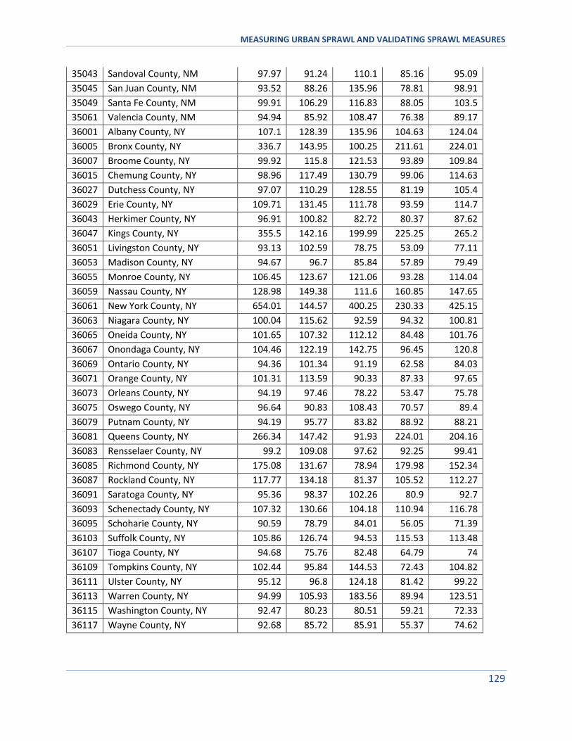
MEASURING URBAN SPRAWL AND VALIDATING SPRAWL MEASURES
129
35043 Sandoval County, NM 97.97 91.24 110.1 85.16 95.09
35045 San Juan County, NM 93.52 88.26 135.96 78.81 98.91
35049 Santa Fe County, NM 99.91 106.29 116.83 88.05 103.5
35061 Valencia County, NM 94.94 85.92 108.47 76.38 89.17
36001 Albany County, NY 107.1 128.39 135.96 104.63 124.04
36005 Bronx County, NY 336.7 143.95 100.25 211.61 224.01
36007 Broome County, NY 99.92 115.8 121.53 93.89 109.84
36015 Chemung County, NY 98.96 117.49 130.79 99.06 114.63
36027 Dutchess County, NY 97.07 110.29 128.55 81.19 105.4
36029 Erie County, NY 109.71 131.45 111.78 93.59 114.7
36043 Herkimer County, NY 96.91 100.82 82.72 80.37 87.62
36047 Kings County, NY 355.5 142.16 199.99 225.25 265.2
36051 Livingston County, NY 93.13 102.59 78.75 53.09 77.11
36053 Madison County, NY 94.67 96.7 85.84 57.89 79.49
36055 Monroe County, NY 106.45 123.67 121.06 93.28 114.04
36059 Nassau County, NY 128.98 149.38 111.6 160.85 147.65
36061 New York County, NY 654.01 144.57 400.25 230.33 425.15
36063 Niagara County, NY 100.04 115.62 92.59 94.32 100.81
36065 Oneida County, NY 101.65 107.32 112.12 84.48 101.76
36067 Onondaga County, NY 104.46 122.19 142.75 96.45 120.8
36069 Ontario County, NY 94.36 101.34 91.19 62.58 84.03
36071 Orange County, NY 101.31 113.59 90.33 87.33 97.65
36073 Orleans County, NY 94.19 97.46 78.22 53.47 75.78
36075 Oswego County, NY 96.64 90.83 108.43 70.57 89.4
36079 Putnam County, NY 94.19 95.77 83.82 88.92 88.21
36081 Queens County, NY 266.34 147.42 91.93 224.01 204.16
36083 Rensselaer County, NY 99.2 109.08 97.62 92.25 99.41
36085 Richmond County, NY 175.08 131.67 78.94 179.98 152.34
36087 Rockland County, NY 117.77 134.18 81.37 105.52 112.27
36091 Saratoga County, NY 95.36 98.37 102.26 80.9 92.7
36093 Schenectady County, NY 107.32 130.66 104.18 110.94 116.78
36095 Schoharie County, NY 90.59 78.79 84.01 56.05 71.39
36103 Suffolk County, NY 105.86 126.74 94.53 115.53 113.48
36107 Tioga County, NY 94.68 75.76 82.48 64.79 74
36109 Tompkins County, NY 102.44 95.84 144.53 72.43 104.82
36111 Ulster County, NY 95.12 96.8 124.18 81.42 99.22
36113 Warren County, NY 94.99 105.93 183.56 89.94 123.51
36115 Washington County, NY 92.47 80.23 80.51 59.21 72.33
36117 Wayne County, NY 92.68 85.72 85.91 55.37 74.62
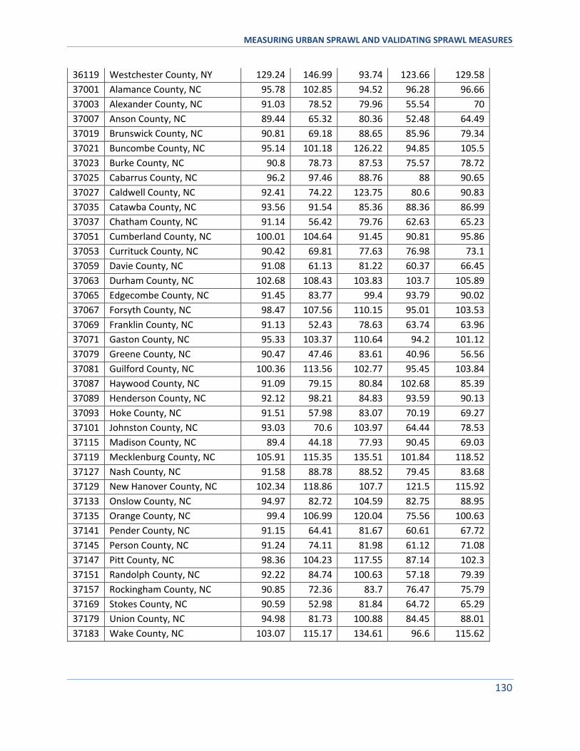
MEASURING URBAN SPRAWL AND VALIDATING SPRAWL MEASURES
130
36119 Westchester County, NY 129.24 146.99 93.74 123.66 129.58
37001 Alamance County, NC 95.78 102.85 94.52 96.28 96.66
37003 Alexander County, NC 91.03 78.52 79.96 55.54 70
37007 Anson County, NC 89.44 65.32 80.36 52.48 64.49
37019 Brunswick County, NC 90.81 69.18 88.65 85.96 79.34
37021 Buncombe County, NC 95.14 101.18 126.22 94.85 105.5
37023 Burke County, NC 90.8 78.73 87.53 75.57 78.72
37025 Cabarrus County, NC 96.2 97.46 88.76 88 90.65
37027 Caldwell County, NC 92.41 74.22 123.75 80.6 90.83
37035 Catawba County, NC 93.56 91.54 85.36 88.36 86.99
37037 Chatham County, NC 91.14 56.42 79.76 62.63 65.23
37051 Cumberland County, NC 100.01 104.64 91.45 90.81 95.86
37053 Currituck County, NC 90.42 69.81 77.63 76.98 73.1
37059 Davie County, NC 91.08 61.13 81.22 60.37 66.45
37063 Durham County, NC 102.68 108.43 103.83 103.7 105.89
37065 Edgecombe County, NC 91.45 83.77 99.4 93.79 90.02
37067 Forsyth County, NC 98.47 107.56 110.15 95.01 103.53
37069 Franklin County, NC 91.13 52.43 78.63 63.74 63.96
37071 Gaston County, NC 95.33 103.37 110.64 94.2 101.12
37079 Greene County, NC 90.47 47.46 83.61 40.96 56.56
37081 Guilford County, NC 100.36 113.56 102.77 95.45 103.84
37087 Haywood County, NC 91.09 79.15 80.84 102.68 85.39
37089 Henderson County, NC 92.12 98.21 84.83 93.59 90.13
37093 Hoke County, NC 91.51 57.98 83.07 70.19 69.27
37101 Johnston County, NC 93.03 70.6 103.97 64.44 78.53
37115 Madison County, NC 89.4 44.18 77.93 90.45 69.03
37119 Mecklenburg County, NC 105.91 115.35 135.51 101.84 118.52
37127 Nash County, NC 91.58 88.78 88.52 79.45 83.68
37129 New Hanover County, NC 102.34 118.86 107.7 121.5 115.92
37133 Onslow County, NC 94.97 82.72 104.59 82.75 88.95
37135 Orange County, NC 99.4 106.99 120.04 75.56 100.63
37141 Pender County, NC 91.15 64.41 81.67 60.61 67.72
37145 Person County, NC 91.24 74.11 81.98 61.12 71.08
37147 Pitt County, NC 98.36 104.23 117.55 87.14 102.3
37151 Randolph County, NC 92.22 84.74 100.63 57.18 79.39
37157 Rockingham County, NC 90.85 72.36 83.7 76.47 75.79
37169 Stokes County, NC 90.59 52.98 81.84 64.72 65.29
37179 Union County, NC 94.98 81.73 100.88 84.45 88.01
37183 Wake County, NC 103.07 115.17 134.61 96.6 115.62
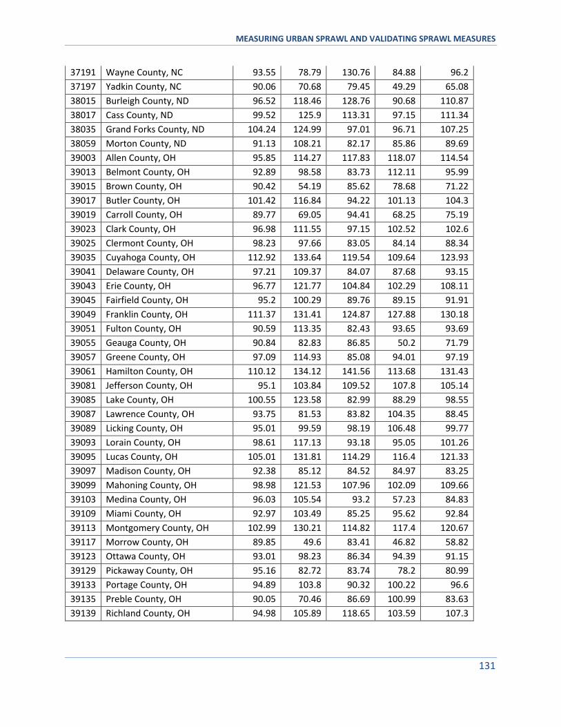
MEASURING URBAN SPRAWL AND VALIDATING SPRAWL MEASURES
131
37191 Wayne County, NC 93.55 78.79 130.76 84.88 96.2
37197 Yadkin County, NC 90.06 70.68 79.45 49.29 65.08
38015 Burleigh County, ND 96.52 118.46 128.76 90.68 110.87
38017 Cass County, ND 99.52 125.9 113.31 97.15 111.34
38035 Grand Forks County, ND 104.24 124.99 97.01 96.71 107.25
38059 Morton County, ND 91.13 108.21 82.17 85.86 89.69
39003 Allen County, OH 95.85 114.27 117.83 118.07 114.54
39013 Belmont County, OH 92.89 98.58 83.73 112.11 95.99
39015 Brown County, OH 90.42 54.19 85.62 78.68 71.22
39017 Butler County, OH 101.42 116.84 94.22 101.13 104.3
39019 Carroll County, OH 89.77 69.05 94.41 68.25 75.19
39023 Clark County, OH 96.98 111.55 97.15 102.52 102.6
39025 Clermont County, OH 98.23 97.66 83.05 84.14 88.34
39035 Cuyahoga County, OH 112.92 133.64 119.54 109.64 123.93
39041 Delaware County, OH 97.21 109.37 84.07 87.68 93.15
39043 Erie County, OH 96.77 121.77 104.84 102.29 108.11
39045 Fairfield County, OH 95.2 100.29 89.76 89.15 91.91
39049 Franklin County, OH 111.37 131.41 124.87 127.88 130.18
39051 Fulton County, OH 90.59 113.35 82.43 93.65 93.69
39055 Geauga County, OH 90.84 82.83 86.85 50.2 71.79
39057 Greene County, OH 97.09 114.93 85.08 94.01 97.19
39061 Hamilton County, OH 110.12 134.12 141.56 113.68 131.43
39081 Jefferson County, OH 95.1 103.84 109.52 107.8 105.14
39085 Lake County, OH 100.55 123.58 82.99 88.29 98.55
39087 Lawrence County, OH 93.75 81.53 83.82 104.35 88.45
39089 Licking County, OH 95.01 99.59 98.19 106.48 99.77
39093 Lorain County, OH 98.61 117.13 93.18 95.05 101.26
39095 Lucas County, OH 105.01 131.81 114.29 116.4 121.33
39097 Madison County, OH 92.38 85.12 84.52 84.97 83.25
39099 Mahoning County, OH 98.98 121.53 107.96 102.09 109.66
39103 Medina County, OH 96.03 105.54 93.2 57.23 84.83
39109 Miami County, OH 92.97 103.49 85.25 95.62 92.84
39113 Montgomery County, OH 102.99 130.21 114.82 117.4 120.67
39117 Morrow County, OH 89.85 49.6 83.41 46.82 58.82
39123 Ottawa County, OH 93.01 98.23 86.34 94.39 91.15
39129 Pickaway County, OH 95.16 82.72 83.74 78.2 80.99
39133 Portage County, OH 94.89 103.8 90.32 100.22 96.6
39135 Preble County, OH 90.05 70.46 86.69 100.99 83.63
39139 Richland County, OH 94.98 105.89 118.65 103.59 107.3
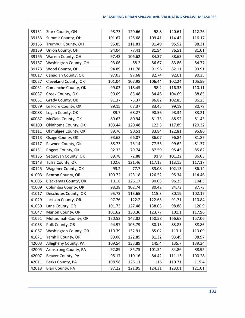
MEASURING URBAN SPRAWL AND VALIDATING SPRAWL MEASURES
132
39151 Stark County, OH 98.73 120.66 98.8 120.61 112.26
39153 Summit County, OH 101.67 125.68 109.41 114.42 116.17
39155 Trumbull County, OH 95.85 111.81 91.49 95.52 98.31
39159 Union County, OH 94.04 77.41 81.94 86.51 81.01
39165 Warren County, OH 97.43 106.62 84.37 88.63 92.75
39167 Washington County, OH 93.06 88.2 86.67 83.86 84.77
39173 Wood County, OH 94.89 111.78 91.96 82.11 93.91
40017 Canadian County, OK 97.03 97.68 82.74 92.01 90.35
40027 Cleveland County, OK 101.04 107.98 106.44 102.24 105.59
40031 Comanche County, OK 99.03 118.45 98.2 116.33 110.11
40037 Creek County, OK 90.09 85.48 84.46 104.69 88.85
40051 Grady County, OK 91.37 75.37 86.82 102.85 86.23
40079 Le Flore County, OK 89.15 67.37 83.45 99.19 80.78
40083 Logan County, OK 89.7 68.27 90.56 98.34 83.21
40087 McClain County, OK 89.63 80.94 81.73 88.92 81.43
40109 Oklahoma County, OK 103.44 120.48 122.5 117.89 120.32
40111 Okmulgee County, OK 89.76 90.51 83.84 122.81 95.86
40113 Osage County, OK 93.63 66.07 86.07 96.84 81.87
40117 Pawnee County, OK 88.73 75.14 77.53 99.62 81.37
40131 Rogers County, OK 92.33 79.74 87.59 95.45 85.82
40135 Sequoyah County, OK 89.78 72.88 91.9 101.22 86.03
40143 Tulsa County, OK 102.6 121.46 117.13 113.15 117.17
40145 Wagoner County, OK 93.2 77.7 83.08 102.13 86.14
41003 Benton County, OR 100.72 123.18 126.52 95.34 114.46
41005 Clackamas County, OR 101.8 126.17 90.03 96.25 104.5
41009 Columbia County, OR 93.28 102.74 80.42 84.73 87.73
41017 Deschutes County, OR 95.73 115.65 115.3 80.19 102.17
41029 Jackson County, OR 97.76 122.2 122.65 91.71 110.84
41039 Lane County, OR 101.73 127.48 138.05 98.88 120.9
41047 Marion County, OR 101.62 130.36 123.77 101.1 117.96
41051 Multnomah County, OR 120.53 142.82 150.58 166.68 157.06
41053 Polk County, OR 94.97 105.79 80.13 83.85 88.86
41067 Washington County, OR 110.39 132.91 85.02 113.1 113.09
41071 Yamhill County, OR 99.08 122.85 81.32 93.49 98.97
42003 Allegheny County, PA 109.54 133.89 145.4 135.7 139.34
42005 Armstrong County, PA 92.89 85.75 101.54 84.86 88.95
42007 Beaver County, PA 95.17 110.16 84.42 111.13 100.28
42011 Berks County, PA 108.58 126.11 116 110.71 119.4
42013 Blair County, PA 97.22 121.95 124.31 123.01 121.01
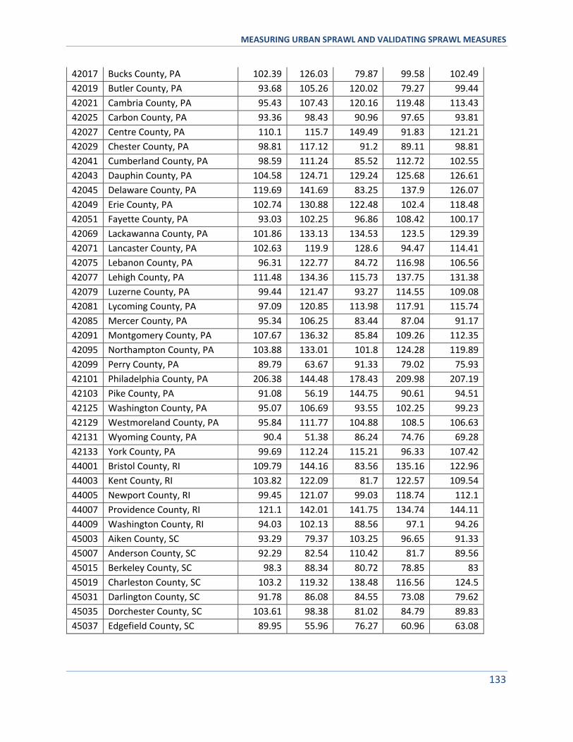
MEASURING URBAN SPRAWL AND VALIDATING SPRAWL MEASURES
133
42017 Bucks County, PA 102.39 126.03 79.87 99.58 102.49
42019 Butler County, PA 93.68 105.26 120.02 79.27 99.44
42021 Cambria County, PA 95.43 107.43 120.16 119.48 113.43
42025 Carbon County, PA 93.36 98.43 90.96 97.65 93.81
42027 Centre County, PA 110.1 115.7 149.49 91.83 121.21
42029 Chester County, PA 98.81 117.12 91.2 89.11 98.81
42041 Cumberland County, PA 98.59 111.24 85.52 112.72 102.55
42043 Dauphin County, PA 104.58 124.71 129.24 125.68 126.61
42045 Delaware County, PA 119.69 141.69 83.25 137.9 126.07
42049 Erie County, PA 102.74 130.88 122.48 102.4 118.48
42051 Fayette County, PA 93.03 102.25 96.86 108.42 100.17
42069 Lackawanna County, PA 101.86 133.13 134.53 123.5 129.39
42071 Lancaster County, PA 102.63 119.9 128.6 94.47 114.41
42075 Lebanon County, PA 96.31 122.77 84.72 116.98 106.56
42077 Lehigh County, PA 111.48 134.36 115.73 137.75 131.38
42079 Luzerne County, PA 99.44 121.47 93.27 114.55 109.08
42081 Lycoming County, PA 97.09 120.85 113.98 117.91 115.74
42085 Mercer County, PA 95.34 106.25 83.44 87.04 91.17
42091 Montgomery County, PA 107.67 136.32 85.84 109.26 112.35
42095 Northampton County, PA 103.88 133.01 101.8 124.28 119.89
42099 Perry County, PA 89.79 63.67 91.33 79.02 75.93
42101 Philadelphia County, PA 206.38 144.48 178.43 209.98 207.19
42103 Pike County, PA 91.08 56.19 144.75 90.61 94.51
42125 Washington County, PA 95.07 106.69 93.55 102.25 99.23
42129 Westmoreland County, PA 95.84 111.77 104.88 108.5 106.63
42131 Wyoming County, PA 90.4 51.38 86.24 74.76 69.28
42133 York County, PA 99.69 112.24 115.21 96.33 107.42
44001 Bristol County, RI 109.79 144.16 83.56 135.16 122.96
44003 Kent County, RI 103.82 122.09 81.7 122.57 109.54
44005 Newport County, RI 99.45 121.07 99.03 118.74 112.1
44007 Providence County, RI 121.1 142.01 141.75 134.74 144.11
44009 Washington County, RI 94.03 102.13 88.56 97.1 94.26
45003 Aiken County, SC 93.29 79.37 103.25 96.65 91.33
45007 Anderson County, SC 92.29 82.54 110.42 81.7 89.56
45015 Berkeley County, SC 98.3 88.34 80.72 78.85 83
45019 Charleston County, SC 103.2 119.32 138.48 116.56 124.5
45031 Darlington County, SC 91.78 86.08 84.55 73.08 79.62
45035 Dorchester County, SC 103.61 98.38 81.02 84.79 89.83
45037 Edgefield County, SC 89.95 55.96 76.27 60.96 63.08
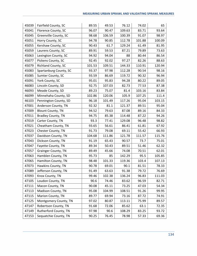
MEASURING URBAN SPRAWL AND VALIDATING SPRAWL MEASURES
134
45039 Fairfield County, SC 89.55 49.53 76.12 74.02 65
45041 Florence County, SC 96.07 90.47 109.63 83.71 93.64
45045 Greenville County, SC 98.68 106.59 100.39 91.07 98.97
45051 Horry County, SC 94.78 90.85 112.78 101.88 100.09
45055 Kershaw County, SC 90.43 61.7 129.24 61.49 81.95
45059 Laurens County, SC 89.91 59.53 87.21 79.89 73.63
45063 Lexington County, SC 94.92 94.04 88 80.44 86.54
45077 Pickens County, SC 92.45 92.02 97.27 82.26 88.63
45079 Richland County, SC 101.53 109.51 144.33 110.91 120.94
45083 Spartanburg County, SC 93.37 97.98 112.28 90.54 98.16
45085 Sumter County, SC 93.59 86.69 119.72 90.32 96.94
45091 York County, SC 95.01 95.83 94.28 80.22 89.05
46083 Lincoln County, SD 92.75 107.03 82.73 77.53 87.38
46093 Meade County, SD 89.23 75.07 81.4 103.16 83.84
46099 Minnehaha County, SD 102.86 120.06 105.9 107.25 111.4
46103 Pennington County, SD 96.18 101.49 117.26 95.04 103.15
47001 Anderson County, TN 92.32 81.1 121.37 89.51 95.04
47009 Blount County, TN 94.52 79.63 87.08 89.16 84.33
47011 Bradley County, TN 94.75 85.38 114.48 87.22 94.26
47019 Carter County, TN 93.3 77.41 129.08 96.48 98.82
47021 Cheatham County, TN 93.65 56.61 86.41 61.81 67.92
47023 Chester County, TN 91.73 79.08 69.11 55.42 66.93
47037 Davidson County, TN 104.68 111.86 121.78 111.57 115.76
47043 Dickson County, TN 91.19 65.43 90.57 73.7 75.01
47047 Fayette County, TN 89.34 50.43 89.51 51.46 62.32
47057 Grainger County, TN 89.49 45.66 74.08 70.51 62.01
47063 Hamblen County, TN 95.73 85 142.29 95.5 105.85
47065 Hamilton County, TN 98.48 101.33 119.36 103.4 107.13
47073 Hawkins County, TN 90.78 69.01 90.1 81.51 78.33
47089 Jefferson County, TN 91.49 63.63 91.38 79.72 76.69
47093 Knox County, TN 99.46 102.38 136.24 96.83 111.03
47105 Loudon County, TN 90.6 74.46 83.62 96.59 82.71
47111 Macon County, TN 90.08 45.11 73.25 47.03 54.34
47113 Madison County, TN 95.08 104.99 108.51 91.26 99.95
47115 Marion County, TN 89.77 69.94 73.16 87.72 74.91
47125 Montgomery County, TN 97.02 80.87 113.11 75.99 89.57
47147 Robertson County, TN 91.68 72.06 85.62 63.1 72.35
47149 Rutherford County, TN 97.98 90.6 108.29 83.25 93.72
47153 Sequatchie County, TN 90.25 76.45 78.98 57.33 69.36
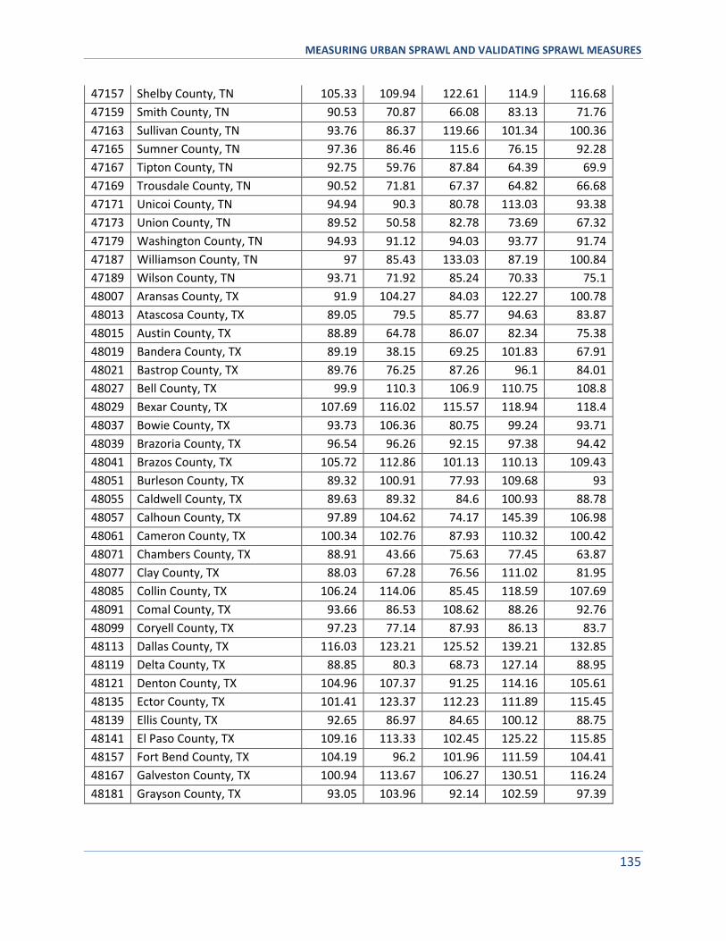
MEASURING URBAN SPRAWL AND VALIDATING SPRAWL MEASURES
135
47157 Shelby County, TN 105.33 109.94 122.61 114.9 116.68
47159 Smith County, TN 90.53 70.87 66.08 83.13 71.76
47163 Sullivan County, TN 93.76 86.37 119.66 101.34 100.36
47165 Sumner County, TN 97.36 86.46 115.6 76.15 92.28
47167 Tipton County, TN 92.75 59.76 87.84 64.39 69.9
47169 Trousdale County, TN 90.52 71.81 67.37 64.82 66.68
47171 Unicoi County, TN 94.94 90.3 80.78 113.03 93.38
47173 Union County, TN 89.52 50.58 82.78 73.69 67.32
47179 Washington County, TN 94.93 91.12 94.03 93.77 91.74
47187 Williamson County, TN 97 85.43 133.03 87.19 100.84
47189 Wilson County, TN 93.71 71.92 85.24 70.33 75.1
48007 Aransas County, TX 91.9 104.27 84.03 122.27 100.78
48013 Atascosa County, TX 89.05 79.5 85.77 94.63 83.87
48015 Austin County, TX 88.89 64.78 86.07 82.34 75.38
48019 Bandera County, TX 89.19 38.15 69.25 101.83 67.91
48021 Bastrop County, TX 89.76 76.25 87.26 96.1 84.01
48027 Bell County, TX 99.9 110.3 106.9 110.75 108.8
48029 Bexar County, TX 107.69 116.02 115.57 118.94 118.4
48037 Bowie County, TX 93.73 106.36 80.75 99.24 93.71
48039 Brazoria County, TX 96.54 96.26 92.15 97.38 94.42
48041 Brazos County, TX 105.72 112.86 101.13 110.13 109.43
48051 Burleson County, TX 89.32 100.91 77.93 109.68 93
48055 Caldwell County, TX 89.63 89.32 84.6 100.93 88.78
48057 Calhoun County, TX 97.89 104.62 74.17 145.39 106.98
48061 Cameron County, TX 100.34 102.76 87.93 110.32 100.42
48071 Chambers County, TX 88.91 43.66 75.63 77.45 63.87
48077 Clay County, TX 88.03 67.28 76.56 111.02 81.95
48085 Collin County, TX 106.24 114.06 85.45 118.59 107.69
48091 Comal County, TX 93.66 86.53 108.62 88.26 92.76
48099 Coryell County, TX 97.23 77.14 87.93 86.13 83.7
48113 Dallas County, TX 116.03 123.21 125.52 139.21 132.85
48119 Delta County, TX 88.85 80.3 68.73 127.14 88.95
48121 Denton County, TX 104.96 107.37 91.25 114.16 105.61
48135 Ector County, TX 101.41 123.37 112.23 111.89 115.45
48139 Ellis County, TX 92.65 86.97 84.65 100.12 88.75
48141 El Paso County, TX 109.16 113.33 102.45 125.22 115.85
48157 Fort Bend County, TX 104.19 96.2 101.96 111.59 104.41
48167 Galveston County, TX 100.94 113.67 106.27 130.51 116.24
48181 Grayson County, TX 93.05 103.96 92.14 102.59 97.39
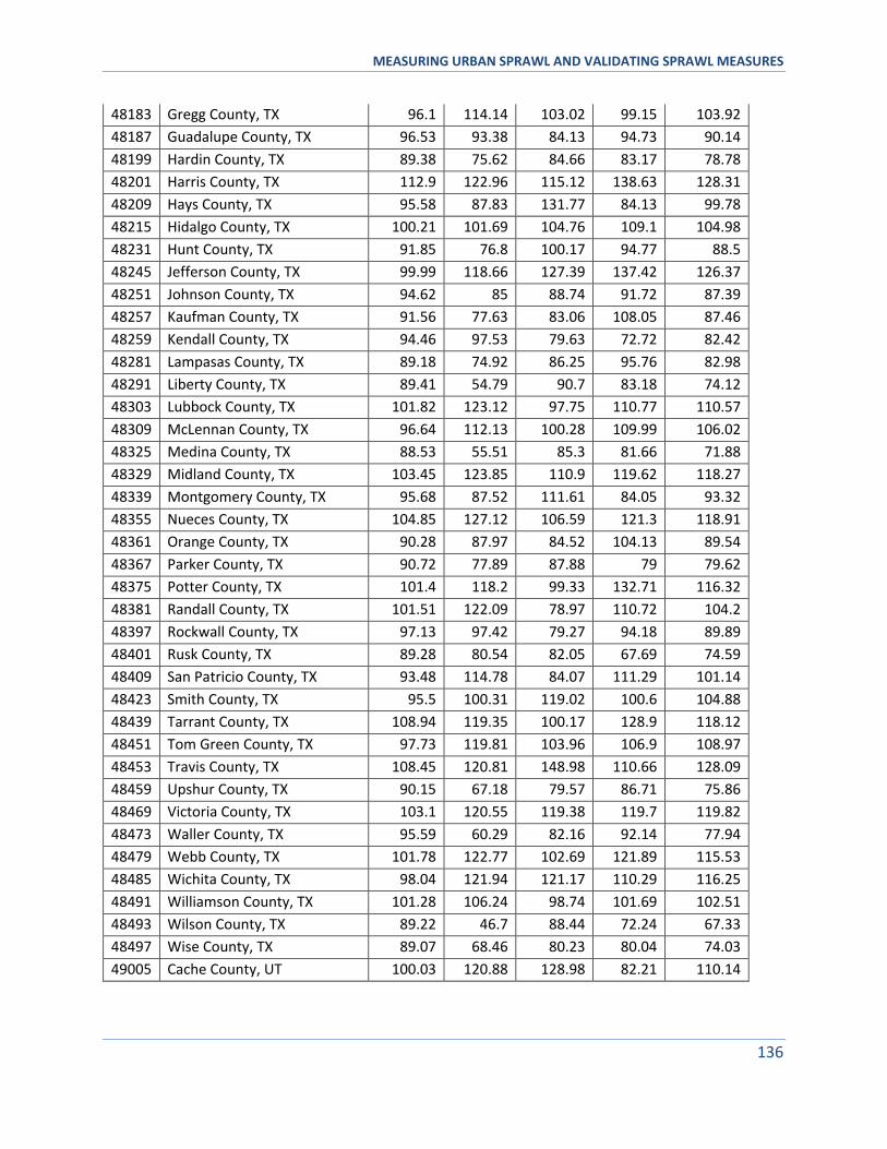
MEASURING URBAN SPRAWL AND VALIDATING SPRAWL MEASURES
136
48183 Gregg County, TX 96.1 114.14 103.02 99.15 103.92
48187 Guadalupe County, TX 96.53 93.38 84.13 94.73 90.14
48199 Hardin County, TX 89.38 75.62 84.66 83.17 78.78
48201 Harris County, TX 112.9 122.96 115.12 138.63 128.31
48209 Hays County, TX 95.58 87.83 131.77 84.13 99.78
48215 Hidalgo County, TX 100.21 101.69 104.76 109.1 104.98
48231 Hunt County, TX 91.85 76.8 100.17 94.77 88.5
48245 Jefferson County, TX 99.99 118.66 127.39 137.42 126.37
48251 Johnson County, TX 94.62 85 88.74 91.72 87.39
48257 Kaufman County, TX 91.56 77.63 83.06 108.05 87.46
48259 Kendall County, TX 94.46 97.53 79.63 72.72 82.42
48281 Lampasas County, TX 89.18 74.92 86.25 95.76 82.98
48291 Liberty County, TX 89.41 54.79 90.7 83.18 74.12
48303 Lubbock County, TX 101.82 123.12 97.75 110.77 110.57
48309 McLennan County, TX 96.64 112.13 100.28 109.99 106.02
48325 Medina County, TX 88.53 55.51 85.3 81.66 71.88
48329 Midland County, TX 103.45 123.85 110.9 119.62 118.27
48339 Montgomery County, TX 95.68 87.52 111.61 84.05 93.32
48355 Nueces County, TX 104.85 127.12 106.59 121.3 118.91
48361 Orange County, TX 90.28 87.97 84.52 104.13 89.54
48367 Parker County, TX 90.72 77.89 87.88 79 79.62
48375 Potter County, TX 101.4 118.2 99.33 132.71 116.32
48381 Randall County, TX 101.51 122.09 78.97 110.72 104.2
48397 Rockwall County, TX 97.13 97.42 79.27 94.18 89.89
48401 Rusk County, TX 89.28 80.54 82.05 67.69 74.59
48409 San Patricio County, TX 93.48 114.78 84.07 111.29 101.14
48423 Smith County, TX 95.5 100.31 119.02 100.6 104.88
48439 Tarrant County, TX 108.94 119.35 100.17 128.9 118.12
48451 Tom Green County, TX 97.73 119.81 103.96 106.9 108.97
48453 Travis County, TX 108.45 120.81 148.98 110.66 128.09
48459 Upshur County, TX 90.15 67.18 79.57 86.71 75.86
48469 Victoria County, TX 103.1 120.55 119.38 119.7 119.82
48473 Waller County, TX 95.59 60.29 82.16 92.14 77.94
48479 Webb County, TX 101.78 122.77 102.69 121.89 115.53
48485 Wichita County, TX 98.04 121.94 121.17 110.29 116.25
48491 Williamson County, TX 101.28 106.24 98.74 101.69 102.51
48493 Wilson County, TX 89.22 46.7 88.44 72.24 67.33
48497 Wise County, TX 89.07 68.46 80.23 80.04 74.03
49005 Cache County, UT 100.03 120.88 128.98 82.21 110.14
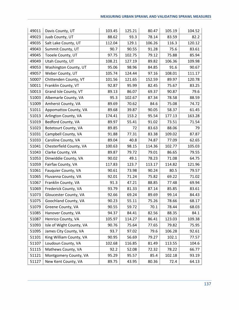
MEASURING URBAN SPRAWL AND VALIDATING SPRAWL MEASURES
137
49011 Davis County, UT 103.45 125.21 80.47 105.19 104.52
49023 Juab County, UT 88.62 93.3 78.14 83.59 82.2
49035 Salt Lake County, UT 112.04 129.1 106.26 116.3 120.12
49043 Summit County, UT 90.7 90.55 91.28 75.6 83.61
49045 Tooele County, UT 97.75 102.75 79.12 75.88 85.94
49049 Utah County, UT 108.21 127.19 89.82 106.36 109.98
49053 Washington County, UT 95.06 98.96 84.85 91.6 90.67
49057 Weber County, UT 105.74 124.44 97.16 108.01 111.17
50007 Chittenden County, VT 101.56 121.65 152.59 89.97 120.78
50011 Franklin County, VT 92.87 95.99 82.45 75.67 83.25
50013 Grand Isle County, VT 89.13 86.07 69.37 90.87 79.6
51003 Albemarle County, VA 95.3 102.67 87.34 78.58 88.59
51009 Amherst County, VA 89.69 70.62 84.6 75.08 74.72
51011 Appomattox County, VA 89.68 39.87 90.05 58.37 61.45
51013 Arlington County, VA 174.41 153.2 95.54 177.13 163.28
51019 Bedford County, VA 89.97 55.41 91.02 73.51 71.54
51023 Botetourt County, VA 89.85 72 83.63 88.06 79
51031 Campbell County, VA 91.88 77.31 83.38 109.02 87.87
51033 Caroline County, VA 89.04 40.8 74.87 77.09 62.65
51041 Chesterfield County, VA 100.63 98.15 114.36 102.77 105.03
51043 Clarke County, VA 89.87 79.72 79.01 86.65 79.55
51053 Dinwiddie County, VA 90.02 49.1 78.23 71.08 64.75
51059 Fairfax County, VA 117.83 123.7 113.17 114.82 121.96
51061 Fauquier County, VA 90.61 73.98 90.24 80.5 79.57
51065 Fluvanna County, VA 92.01 71.24 75.82 69.22 71.02
51067 Franklin County, VA 91.3 47.21 88.85 77.48 69.94
51069 Frederick County, VA 93.79 81.33 87.14 85.85 83.61
51073 Gloucester County, VA 92.66 69.24 89.69 99.14 84.43
51075 Goochland County, VA 90.23 55.11 75.26 78.66 68.17
51079 Greene County, VA 90.55 59.72 70.1 78.44 68.03
51085 Hanover County, VA 94.37 84.41 82.56 88.35 84.1
51087 Henrico County, VA 105.97 114.27 86.41 123.03 109.38
51093 Isle of Wight County, VA 90.76 75.64 77.65 79.82 75.95
51095 James City County, VA 93.7 97.02 79.6 106.28 92.61
51101 King William County, VA 90.95 56.69 79.27 102.1 77.57
51107 Loudoun County, VA 102.68 116.85 81.49 113.55 104.6
51115 Mathews County, VA 92.2 52.08 72.32 78.22 66.77
51121 Montgomery County, VA 95.29 95.57 85.4 102.18 93.19
51127 New Kent County, VA 89.75 43.95 80.36 72.4 64.13
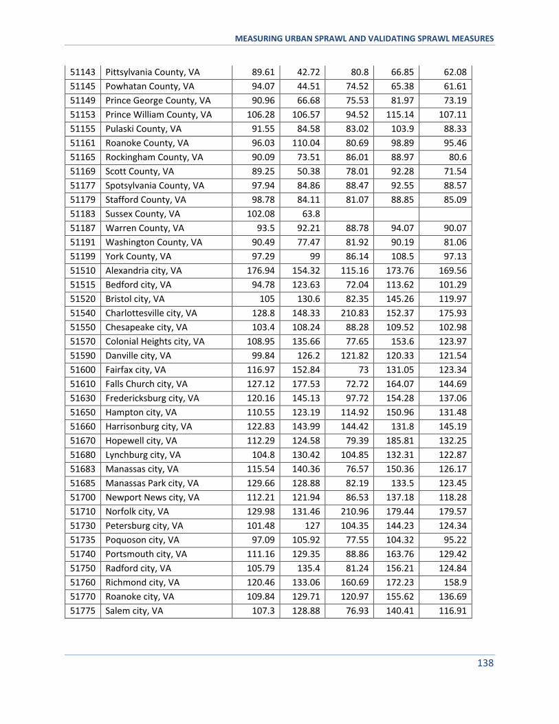
MEASURING URBAN SPRAWL AND VALIDATING SPRAWL MEASURES
138
51143 Pittsylvania County, VA 89.61 42.72 80.8 66.85 62.08
51145 Powhatan County, VA 94.07 44.51 74.52 65.38 61.61
51149 Prince George County, VA 90.96 66.68 75.53 81.97 73.19
51153 Prince William County, VA 106.28 106.57 94.52 115.14 107.11
51155 Pulaski County, VA 91.55 84.58 83.02 103.9 88.33
51161 Roanoke County, VA 96.03 110.04 80.69 98.89 95.46
51165 Rockingham County, VA 90.09 73.51 86.01 88.97 80.6
51169 Scott County, VA 89.25 50.38 78.01 92.28 71.54
51177 Spotsylvania County, VA 97.94 84.86 88.47 92.55 88.57
51179 Stafford County, VA 98.78 84.11 81.07 88.85 85.09
51183 Sussex County, VA 102.08 63.8
51187 Warren County, VA 93.5 92.21 88.78 94.07 90.07
51191 Washington County, VA 90.49 77.47 81.92 90.19 81.06
51199 York County, VA 97.29 99 86.14 108.5 97.13
51510 Alexandria city, VA 176.94 154.32 115.16 173.76 169.56
51515 Bedford city, VA 94.78 123.63 72.04 113.62 101.29
51520 Bristol city, VA 105 130.6 82.35 145.26 119.97
51540 Charlottesville city, VA 128.8 148.33 210.83 152.37 175.93
51550 Chesapeake city, VA 103.4 108.24 88.28 109.52 102.98
51570 Colonial Heights city, VA 108.95 135.66 77.65 153.6 123.97
51590 Danville city, VA 99.84 126.2 121.82 120.33 121.54
51600 Fairfax city, VA 116.97 152.84 73 131.05 123.34
51610 Falls Church city, VA 127.12 177.53 72.72 164.07 144.69
51630 Fredericksburg city, VA 120.16 145.13 97.72 154.28 137.06
51650 Hampton city, VA 110.55 123.19 114.92 150.96 131.48
51660 Harrisonburg city, VA 122.83 143.99 144.42 131.8 145.19
51670 Hopewell city, VA 112.29 124.58 79.39 185.81 132.25
51680 Lynchburg city, VA 104.8 130.42 104.85 132.31 122.87
51683 Manassas city, VA 115.54 140.36 76.57 150.36 126.17
51685 Manassas Park city, VA 129.66 128.88 82.19 133.5 123.45
51700 Newport News city, VA 112.21 121.94 86.53 137.18 118.28
51710 Norfolk city, VA 129.98 131.46 210.96 179.44 179.57
51730 Petersburg city, VA 101.48 127 104.35 144.23 124.34
51735 Poquoson city, VA 97.09 105.92 77.55 104.32 95.22
51740 Portsmouth city, VA 111.16 129.35 88.86 163.76 129.42
51750 Radford city, VA 105.79 135.4 81.24 156.21 124.84
51760 Richmond city, VA 120.46 133.06 160.69 172.23 158.9
51770 Roanoke city, VA 109.84 129.71 120.97 155.62 136.69
51775 Salem city, VA 107.3 128.88 76.93 140.41 116.91
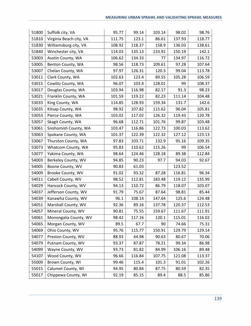
MEASURING URBAN SPRAWL AND VALIDATING SPRAWL MEASURES
139
51800 Suffolk city, VA 95.77 99.14 103.14 98.02 98.76
51810 Virginia Beach city, VA 111.75 123.1 86.61 137.93 118.77
51830 Williamsburg city, VA 108.92 118.37 158.9 136.03 138.61
51840 Winchester city, VA 114.03 135.13 133.91 150.19 142.1
53003 Asotin County, WA 106.62 134.33 77 134.97 116.72
53005 Benton County, WA 98.56 118.73 109.61 97.28 107.64
53007 Chelan County, WA 97.97 126.31 120.3 99.04 113.78
53011 Clark County, WA 102.63 123.4 89.55 105.28 106.59
53015 Cowlitz County, WA 96.07 103.4 128.01 99 108.37
53017 Douglas County, WA 103.94 116.98 82.17 91.3 98.23
53021 Franklin County, WA 101.59 119.22 82.23 111.14 104.48
53033 King County, WA 114.85 128.93 159.34 131.7 142.6
53035 Kitsap County, WA 98.92 107.82 115.62 96.04 105.81
53053 Pierce County, WA 103.02 117.02 126.32 119.43 120.78
53057 Skagit County, WA 96.68 112.71 101.76 99.87 103.48
53061 Snohomish County, WA 103.47 116.86 122.73 100.03 113.62
53063 Spokane County, WA 101.37 122.39 122.32 127.12 123.13
53067 Thurston County, WA 97.83 103.71 132.9 95.16 109.35
53073 Whatcom County, WA 95.83 110.62 115.26 99 106.54
53077 Yakima County, WA 98.64 124.46 128.18 89.38 112.84
54003 Berkeley County, WV 94.85 90.23 97.7 94.03 92.67
54005 Boone County, WV 90.83 61.03 123.52
54009 Brooke County, WV 91.02 93.32 87.28 116.81 96.34
54011 Cabell County, WV 98.52 112.81 183.48 119.12 135.99
54029 Hancock County, WV 94.13 110.72 86.79 118.07 103.07
54037 Jefferson County, WV 91.79 75.67 87.64 98.81 85.44
54039 Kanawha County, WV 96.1 108.14 147.64 125.6 124.48
54051 Marshall County, WV 92.36 89.16 137.78 120.37 112.53
54057 Mineral County, WV 90.81 75.55 159.67 111.67 111.91
54061 Monongalia County, WV 98.42 117.16 120.1 115.01 116.02
54065 Morgan County, WV 89.5 67.7 90 74.66 75.31
54069 Ohio County, WV 95.76 115.77 150.91 129.79 129.14
54077 Preston County, WV 88.93 44.98 90.63 80.67 70.06
54079 Putnam County, WV 93.37 87.87 78.21 99.34 86.98
54099 Wayne County, WV 93.73 81.82 84.99 106.16 89.48
54107 Wood County, WV 96.66 116.84 107.75 121.08 113.37
55009 Brown County, WI 99.46 115.4 101.3 91.01 102.26
55015 Calumet County, WI 94.95 80.84 87.75 80.59 82.35
55017 Chippewa County, WI 92.19 85.15 89.4 88.5 85.86
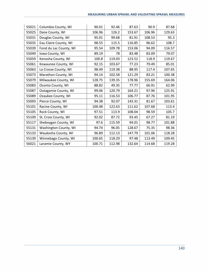
MEASURING URBAN SPRAWL AND VALIDATING SPRAWL MEASURES
140
55021 Columbia County, WI 90.01 92.46 87.63 90.9 87.68
55025 Dane County, WI 106.96 126.2 153.67 106.96 129.63
55031 Douglas County, WI 95.01 99.68 81.91 108.53 95.3
55035 Eau Claire County, WI 98.55 115.5 116.85 96.62 108.7
55039 Fond du Lac County, WI 95.54 109.78 153.06 94.09 116.57
55049 Iowa County, WI 89.19 78 83.48 83.09 79.07
55059 Kenosha County, WI 100.8 119.03 123.52 118.9 119.67
55061 Kewaunee County, WI 92.15 103.67 77.23 79.49 85.01
55063 La Crosse County, WI 98.49 119.38 88.95 117.4 107.65
55073 Marathon County, WI 94.14 102.58 121.29 83.21 100.38
55079 Milwaukee County, WI 128.75 139.35 178.96 155.69 164.06
55083 Oconto County, WI 88.82 49.35 77.77 66.91 62.99
55087 Outagamie County, WI 99.06 120.79 164.21 97.96 125.91
55089 Ozaukee County, WI 95.11 116.53 106.77 87.76 101.95
55093 Pierce County, WI 94.38 92.07 143.31 81.67 103.61
55101 Racine County, WI 100.48 122.63 111.62 107.68 113.4
55105 Rock County, WI 97.51 113.9 108.04 98.59 105.7
55109 St. Croix County, WI 92.02 87.72 93.45 67.27 81.19
55117 Sheboygan County, WI 97.6 115.59 94.01 98.77 101.88
55131 Washington County, WI 94.74 96.05 128.67 75.35 98.36
55133 Waukesha County, WI 96.89 112.13 147.79 101.06 118.28
55139 Winnebago County, WI 100.65 118.29 97.48 113.49 109.45
56021 Laramie County, WY 100.71 112.98 132.64 114.68 119.28
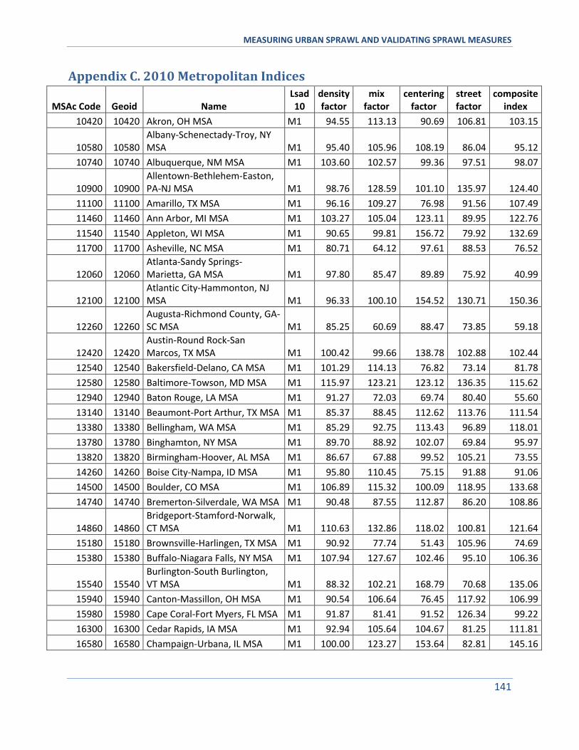
MEASURING URBAN SPRAWL AND VALIDATING SPRAWL MEASURES
141
Appendix C. 2010 Metropolitan Indices
MSAc Code Geoid Name Lsad 10
density factor
mix factor
centering factor
street factor
composite index
10420 10420 Akron, OH MSA M1 94.55 113.13 90.69 106.81 103.15
10580 10580 Albany-Schenectady-Troy, NY MSA M1 95.40 105.96 108.19 86.04 95.12
10740 10740 Albuquerque, NM MSA M1 103.60 102.57 99.36 97.51 98.07
10900 10900 Allentown-Bethlehem-Easton, PA-NJ MSA M1 98.76 128.59 101.10 135.97 124.40
11100 11100 Amarillo, TX MSA M1 96.16 109.27 76.98 91.56 107.49
11460 11460 Ann Arbor, MI MSA M1 103.27 105.04 123.11 89.95 122.76
11540 11540 Appleton, WI MSA M1 90.65 99.81 156.72 79.92 132.69
11700 11700 Asheville, NC MSA M1 80.71 64.12 97.61 88.53 76.52
12060 12060 Atlanta-Sandy Springs-Marietta, GA MSA M1 97.80 85.47 89.89 75.92 40.99
12100 12100 Atlantic City-Hammonton, NJ MSA M1 96.33 100.10 154.52 130.71 150.36
12260 12260 Augusta-Richmond County, GA-SC MSA M1 85.25 60.69 88.47 73.85 59.18
12420 12420 Austin-Round Rock-San Marcos, TX MSA M1 100.42 99.66 138.78 102.88 102.44
12540 12540 Bakersfield-Delano, CA MSA M1 101.29 114.13 76.82 73.14 81.78
12580 12580 Baltimore-Towson, MD MSA M1 115.97 123.21 123.12 136.35 115.62
12940 12940 Baton Rouge, LA MSA M1 91.27 72.03 69.74 80.40 55.60
13140 13140 Beaumont-Port Arthur, TX MSA M1 85.37 88.45 112.62 113.76 111.54
13380 13380 Bellingham, WA MSA M1 85.29 92.75 113.43 96.89 118.01
13780 13780 Binghamton, NY MSA M1 89.70 88.92 102.07 69.84 95.97
13820 13820 Birmingham-Hoover, AL MSA M1 86.67 67.88 99.52 105.21 73.55
14260 14260 Boise City-Nampa, ID MSA M1 95.80 110.45 75.15 91.88 91.06
14500 14500 Boulder, CO MSA M1 106.89 115.32 100.09 118.95 133.68
14740 14740 Bremerton-Silverdale, WA MSA M1 90.48 87.55 112.87 86.20 108.86
14860 14860 Bridgeport-Stamford-Norwalk, CT MSA M1 110.63 132.86 118.02 100.81 121.64
15180 15180 Brownsville-Harlingen, TX MSA M1 90.92 77.74 51.43 105.96 74.69
15380 15380 Buffalo-Niagara Falls, NY MSA M1 107.94 127.67 102.46 95.10 106.36
15540 15540 Burlington-South Burlington, VT MSA M1 88.32 102.21 168.79 70.68 135.06
15940 15940 Canton-Massillon, OH MSA M1 90.54 106.64 76.45 117.92 106.99
15980 15980 Cape Coral-Fort Myers, FL MSA M1 91.87 81.41 91.52 126.34 99.22
16300 16300 Cedar Rapids, IA MSA M1 92.94 105.64 104.67 81.25 111.81
16580 16580 Champaign-Urbana, IL MSA M1 100.00 123.27 153.64 82.81 145.16
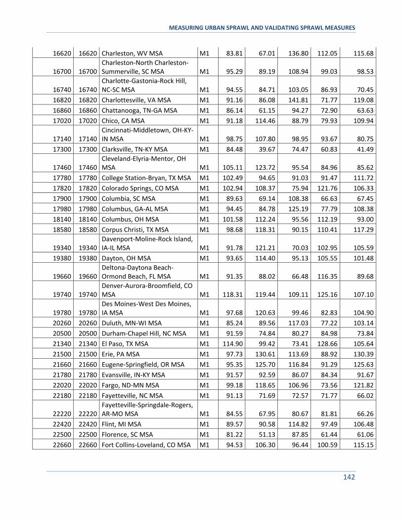
MEASURING URBAN SPRAWL AND VALIDATING SPRAWL MEASURES
142
16620 16620 Charleston, WV MSA M1 83.81 67.01 136.80 112.05 115.68
16700 16700 Charleston-North Charleston-Summerville, SC MSA M1 95.29 89.19 108.94 99.03 98.53
16740 16740 Charlotte-Gastonia-Rock Hill, NC-SC MSA M1 94.55 84.71 103.05 86.93 70.45
16820 16820 Charlottesville, VA MSA M1 91.16 86.08 141.81 71.77 119.08
16860 16860 Chattanooga, TN-GA MSA M1 86.14 61.15 94.27 72.90 63.63
17020 17020 Chico, CA MSA M1 91.18 114.46 88.79 79.93 109.94
17140 17140 Cincinnati-Middletown, OH-KY-IN MSA M1 98.75 107.80 98.95 93.67 80.75
17300 17300 Clarksville, TN-KY MSA M1 84.48 39.67 74.47 60.83 41.49
17460 17460 Cleveland-Elyria-Mentor, OH MSA M1 105.11 123.72 95.54 84.96 85.62
17780 17780 College Station-Bryan, TX MSA M1 102.49 94.65 91.03 91.47 111.72
17820 17820 Colorado Springs, CO MSA M1 102.94 108.37 75.94 121.76 106.33
17900 17900 Columbia, SC MSA M1 89.63 69.14 108.38 66.63 67.45
17980 17980 Columbus, GA-AL MSA M1 94.45 84.78 125.19 77.79 108.38
18140 18140 Columbus, OH MSA M1 101.58 112.24 95.56 112.19 93.00
18580 18580 Corpus Christi, TX MSA M1 98.68 118.31 90.15 110.41 117.29
19340 19340 Davenport-Moline-Rock Island, IA-IL MSA M1 91.78 121.21 70.03 102.95 105.59
19380 19380 Dayton, OH MSA M1 93.65 114.40 95.13 105.55 101.48
19660 19660 Deltona-Daytona Beach-Ormond Beach, FL MSA M1 91.35 88.02 66.48 116.35 89.68
19740 19740 Denver-Aurora-Broomfield, CO MSA M1 118.31 119.44 109.11 125.16 107.10
19780 19780 Des Moines-West Des Moines, IA MSA M1 97.68 120.63 99.46 82.83 104.90
20260 20260 Duluth, MN-WI MSA M1 85.24 89.56 117.03 77.22 103.14
20500 20500 Durham-Chapel Hill, NC MSA M1 91.59 74.84 80.27 84.98 73.84
21340 21340 El Paso, TX MSA M1 114.90 99.42 73.41 128.66 105.64
21500 21500 Erie, PA MSA M1 97.73 130.61 113.69 88.92 130.39
21660 21660 Eugene-Springfield, OR MSA M1 95.35 125.70 116.84 91.29 125.63
21780 21780 Evansville, IN-KY MSA M1 91.57 92.59 86.07 84.34 91.67
22020 22020 Fargo, ND-MN MSA M1 99.18 118.65 106.96 73.56 121.82
22180 22180 Fayetteville, NC MSA M1 91.13 71.69 72.57 71.77 66.02
22220 22220 Fayetteville-Springdale-Rogers, AR-MO MSA M1 84.55 67.95 80.67 81.81 66.26
22420 22420 Flint, MI MSA M1 89.57 90.58 114.82 97.49 106.48
22500 22500 Florence, SC MSA M1 81.22 51.13 87.85 61.44 61.06
22660 22660 Fort Collins-Loveland, CO MSA M1 94.53 106.30 96.44 100.59 115.15
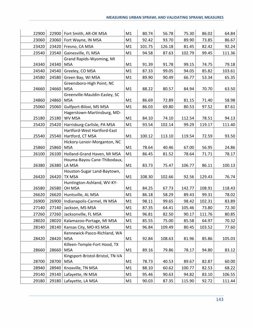
MEASURING URBAN SPRAWL AND VALIDATING SPRAWL MEASURES
143
22900 22900 Fort Smith, AR-OK MSA M1 80.74 56.78 75.30 86.02 64.84
23060 23060 Fort Wayne, IN MSA M1 92.42 93.70 89.90 73.85 86.67
23420 23420 Fresno, CA MSA M1 101.75 126.18 81.45 82.42 92.24
23540 23540 Gainesville, FL MSA M1 94.58 87.63 102.79 99.45 111.36
24340 24340 Grand Rapids-Wyoming, MI MSA M1 91.39 91.78 99.15 74.75 79.18
24540 24540 Greeley, CO MSA M1 87.33 99.05 94.05 85.82 103.61
24580 24580 Green Bay, WI MSA M1 89.90 90.49 66.77 53.34 65.35
24660 24660 Greensboro-High Point, NC MSA M1 88.22 80.57 84.94 70.70 63.50
24860 24860 Greenville-Mauldin-Easley, SC MSA M1 86.69 72.89 81.15 71.40 58.98
25060 25060 Gulfport-Biloxi, MS MSA M1 86.03 69.80 80.53 97.52 87.61
25180 25180 Hagerstown-Martinsburg, MD-WV MSA M1 84.10 74.10 112.54 78.51 94.13
25420 25420 Harrisburg-Carlisle, PA MSA M1 93.54 102.14 99.29 119.17 111.40
25540 25540 Hartford-West Hartford-East Hartford, CT MSA M1 100.12 113.10 119.54 72.59 93.50
25860 25860 Hickory-Lenoir-Morganton, NC MSA M1 78.64 40.46 67.00 56.95 24.86
26100 26100 Holland-Grand Haven, MI MSA M1 86.45 81.52 78.64 71.71 78.17
26380 26380 Houma-Bayou Cane-Thibodaux, LA MSA M1 83.73 75.47 106.77 86.11 100.13
26420 26420 Houston-Sugar Land-Baytown, TX MSA M1 108.30 102.66 92.56 129.43 76.74
26580 26580 Huntington-Ashland, WV-KY-OH MSA M1 84.25 67.73 142.77 108.91 118.43
26620 26620 Huntsville, AL MSA M1 86.18 58.29 89.43 99.31 78.02
26900 26900 Indianapolis-Carmel, IN MSA M1 98.11 99.65 98.42 102.31 83.89
27140 27140 Jackson, MS MSA M1 87.35 64.41 105.46 73.80 72.30
27260 27260 Jacksonville, FL MSA M1 96.81 82.50 90.17 111.76 80.85
28020 28020 Kalamazoo-Portage, MI MSA M1 85.55 75.00 85.58 64.97 70.32
28140 28140 Kansas City, MO-KS MSA M1 96.84 109.49 80.45 103.52 77.60
28420 28420 Kennewick-Pasco-Richland, WA MSA M1 92.84 108.63 81.96 85.86 105.03
28660 28660 Killeen-Temple-Fort Hood, TX MSA M1 89.16 79.86 78.17 94.80 83.12
28700 28700 Kingsport-Bristol-Bristol, TN-VA MSA M1 78.73 40.53 89.67 82.87 60.00
28940 28940 Knoxville, TN MSA M1 88.10 60.62 100.77 82.53 68.22
29140 29140 Lafayette, IN MSA M1 95.46 90.63 94.82 83.10 106.55
29180 29180 Lafayette, LA MSA M1 90.03 87.35 115.90 92.72 111.44
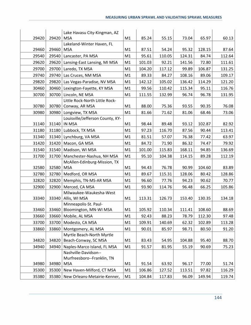
MEASURING URBAN SPRAWL AND VALIDATING SPRAWL MEASURES
144
29420 29420 Lake Havasu City-Kingman, AZ MSA M1 85.24 55.15 73.04 65.97 60.13
29460 29460 Lakeland-Winter Haven, FL MSA M1 87.51 54.24 95.32 128.15 87.64
29540 29540 Lancaster, PA MSA M1 95.61 110.05 124.31 84.74 112.64
29620 29620 Lansing-East Lansing, MI MSA M1 101.03 92.21 141.56 72.80 111.61
29700 29700 Laredo, TX MSA M1 104.20 117.12 99.89 106.87 131.25
29740 29740 Las Cruces, NM MSA M1 89.33 84.27 108.16 89.06 109.17
29820 29820 Las Vegas-Paradise, NV MSA M1 142.12 105.02 136.42 114.29 121.20
30460 30460 Lexington-Fayette, KY MSA M1 99.56 110.42 115.34 95.11 116.76
30700 30700 Lincoln, NE MSA M1 111.55 132.99 96.74 96.78 131.95
30780 30780 Little Rock-North Little Rock-Conway, AR MSA M1 88.00 75.36 93.55 90.35 76.08
30980 30980 Longview, TX MSA M1 81.66 71.62 81.06 68.46 73.06
31140 31140 Louisville/Jefferson County, KY-IN MSA M1 98.44 89.48 93.12 102.87 82.92
31180 31180 Lubbock, TX MSA M1 97.23 116.70 87.56 90.44 113.41
31340 31340 Lynchburg, VA MSA M1 81.51 57.07 76.38 77.42 63.97
31420 31420 Macon, GA MSA M1 84.72 71.90 86.32 74.47 79.92
31540 31540 Madison, WI MSA M1 101.00 115.83 168.11 94.85 136.69
31700 31700 Manchester-Nashua, NH MSA M1 95.10 104.38 114.15 89.28 112.19
32580 32580 McAllen-Edinburg-Mission, TX MSA M1 94.43 76.78 90.99 104.60 83.89
32780 32780 Medford, OR MSA M1 89.67 115.31 128.06 80.42 128.86
32820 32820 Memphis, TN-MS-AR MSA M1 96.60 77.76 94.23 90.62 70.77
32900 32900 Merced, CA MSA M1 93.90 114.76 96.48 66.25 105.86
33340 33340 Milwaukee-Waukesha-West Allis, WI MSA M1 113.31 126.73 153.40 130.35 134.18
33460 33460 Minneapolis-St. Paul-Bloomington, MN-WI MSA M1 105.92 110.34 111.41 108.60 88.69
33660 33660 Mobile, AL MSA M1 92.43 88.23 78.79 112.30 97.48
33700 33700 Modesto, CA MSA M1 109.91 140.69 62.32 102.89 113.28
33860 33860 Montgomery, AL MSA M1 90.01 85.97 98.71 80.50 91.20
34820 34820 Myrtle Beach-North Myrtle Beach-Conway, SC MSA M1 83.43 54.95 104.88 95.40 88.70
34940 34940 Naples-Marco Island, FL MSA M1 91.57 81.95 55.19 90.69 75.23
34980 34980
Nashville-Davidson--Murfreesboro--Franklin, TN MSA M1 91.54 63.92 96.17 77.00 51.74
35300 35300 New Haven-Milford, CT MSA M1 106.86 127.52 113.51 97.82 116.29
35380 35380 New Orleans-Metairie-Kenner, M1 104.84 117.83 96.09 149.94 119.74
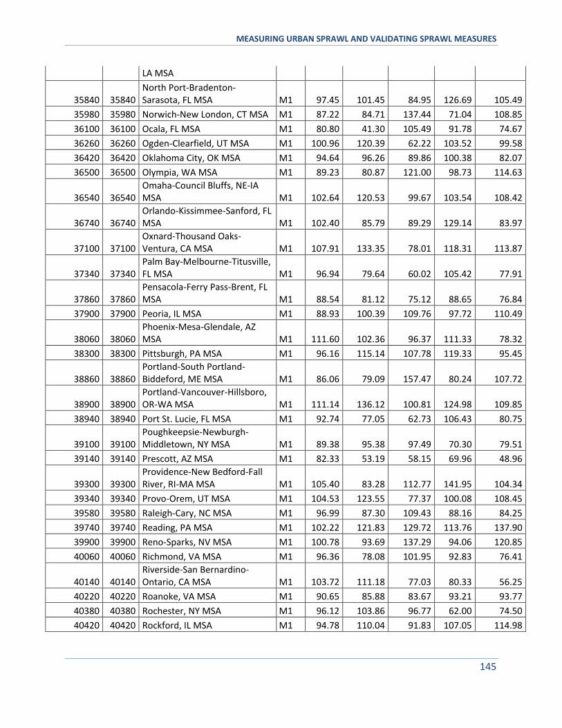
MEASURING URBAN SPRAWL AND VALIDATING SPRAWL MEASURES
145
LA MSA
35840 35840 North Port-Bradenton-Sarasota, FL MSA M1 97.45 101.45 84.95 126.69 105.49
35980 35980 Norwich-New London, CT MSA M1 87.22 84.71 137.44 71.04 108.85
36100 36100 Ocala, FL MSA M1 80.80 41.30 105.49 91.78 74.67
36260 36260 Ogden-Clearfield, UT MSA M1 100.96 120.39 62.22 103.52 99.58
36420 36420 Oklahoma City, OK MSA M1 94.64 96.26 89.86 100.38 82.07
36500 36500 Olympia, WA MSA M1 89.23 80.87 121.00 98.73 114.63
36540 36540 Omaha-Council Bluffs, NE-IA MSA M1 102.64 120.53 99.67 103.54 108.42
36740 36740 Orlando-Kissimmee-Sanford, FL MSA M1 102.40 85.79 89.29 129.14 83.97
37100 37100 Oxnard-Thousand Oaks-Ventura, CA MSA M1 107.91 133.35 78.01 118.31 113.87
37340 37340 Palm Bay-Melbourne-Titusville, FL MSA M1 96.94 79.64 60.02 105.42 77.91
37860 37860 Pensacola-Ferry Pass-Brent, FL MSA M1 88.54 81.12 75.12 88.65 76.84
37900 37900 Peoria, IL MSA M1 88.93 100.39 109.76 97.72 110.49
38060 38060 Phoenix-Mesa-Glendale, AZ MSA M1 111.60 102.36 96.37 111.33 78.32
38300 38300 Pittsburgh, PA MSA M1 96.16 115.14 107.78 119.33 95.45
38860 38860 Portland-South Portland-Biddeford, ME MSA M1 86.06 79.09 157.47 80.24 107.72
38900 38900 Portland-Vancouver-Hillsboro, OR-WA MSA M1 111.14 136.12 100.81 124.98 109.85
38940 38940 Port St. Lucie, FL MSA M1 92.74 77.05 62.73 106.43 80.75
39100 39100 Poughkeepsie-Newburgh-Middletown, NY MSA M1 89.38 95.38 97.49 70.30 79.51
39140 39140 Prescott, AZ MSA M1 82.33 53.19 58.15 69.96 48.96
39300 39300 Providence-New Bedford-Fall River, RI-MA MSA M1 105.40 83.28 112.77 141.95 104.34
39340 39340 Provo-Orem, UT MSA M1 104.53 123.55 77.37 100.08 108.45
39580 39580 Raleigh-Cary, NC MSA M1 96.99 87.30 109.43 88.16 84.25
39740 39740 Reading, PA MSA M1 102.22 121.83 129.72 113.76 137.90
39900 39900 Reno-Sparks, NV MSA M1 100.78 93.69 137.29 94.06 120.85
40060 40060 Richmond, VA MSA M1 96.36 78.08 101.95 92.83 76.41
40140 40140 Riverside-San Bernardino-Ontario, CA MSA M1 103.72 111.18 77.03 80.33 56.25
40220 40220 Roanoke, VA MSA M1 90.65 85.88 83.67 93.21 93.77
40380 40380 Rochester, NY MSA M1 96.12 103.86 96.77 62.00 74.50
40420 40420 Rockford, IL MSA M1 94.78 110.04 91.83 107.05 114.98
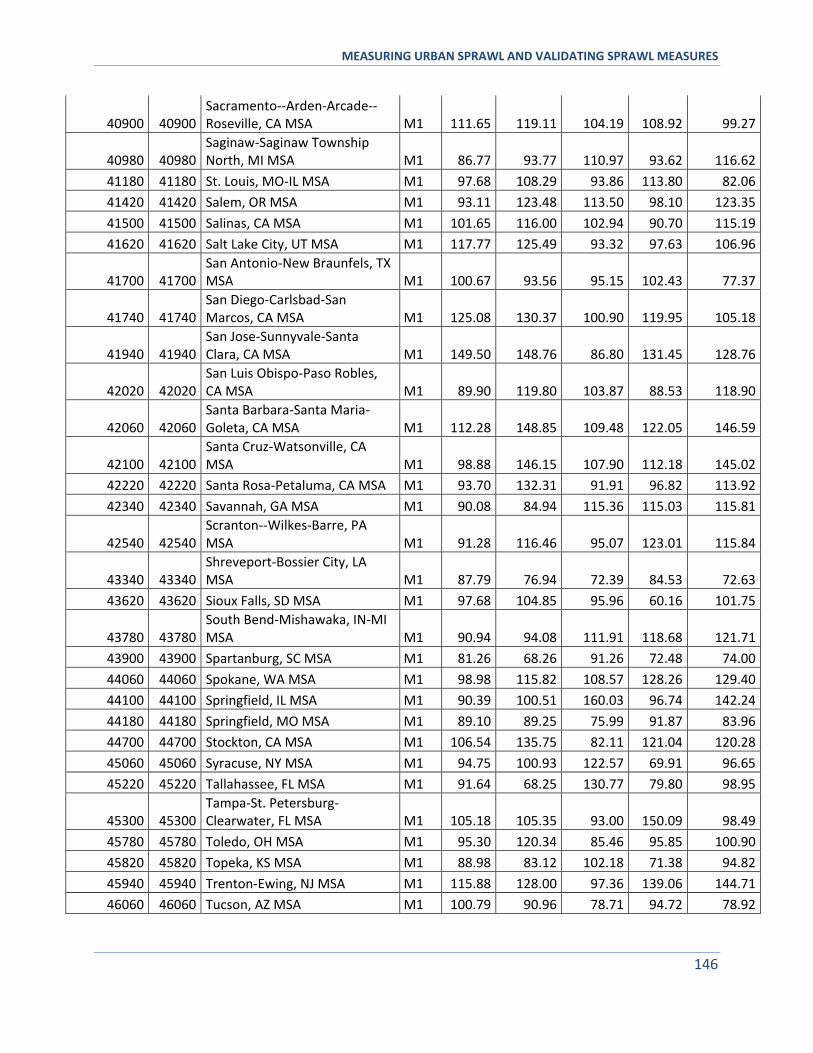
MEASURING URBAN SPRAWL AND VALIDATING SPRAWL MEASURES
146
40900 40900 Sacramento--Arden-Arcade--Roseville, CA MSA M1 111.65 119.11 104.19 108.92 99.27
40980 40980 Saginaw-Saginaw Township North, MI MSA M1 86.77 93.77 110.97 93.62 116.62
41180 41180 St. Louis, MO-IL MSA M1 97.68 108.29 93.86 113.80 82.06
41420 41420 Salem, OR MSA M1 93.11 123.48 113.50 98.10 123.35
41500 41500 Salinas, CA MSA M1 101.65 116.00 102.94 90.70 115.19
41620 41620 Salt Lake City, UT MSA M1 117.77 125.49 93.32 97.63 106.96
41700 41700 San Antonio-New Braunfels, TX MSA M1 100.67 93.56 95.15 102.43 77.37
41740 41740 San Diego-Carlsbad-San Marcos, CA MSA M1 125.08 130.37 100.90 119.95 105.18
41940 41940 San Jose-Sunnyvale-Santa Clara, CA MSA M1 149.50 148.76 86.80 131.45 128.76
42020 42020 San Luis Obispo-Paso Robles, CA MSA M1 89.90 119.80 103.87 88.53 118.90
42060 42060 Santa Barbara-Santa Maria-Goleta, CA MSA M1 112.28 148.85 109.48 122.05 146.59
42100 42100 Santa Cruz-Watsonville, CA MSA M1 98.88 146.15 107.90 112.18 145.02
42220 42220 Santa Rosa-Petaluma, CA MSA M1 93.70 132.31 91.91 96.82 113.92
42340 42340 Savannah, GA MSA M1 90.08 84.94 115.36 115.03 115.81
42540 42540 Scranton--Wilkes-Barre, PA MSA M1 91.28 116.46 95.07 123.01 115.84
43340 43340 Shreveport-Bossier City, LA MSA M1 87.79 76.94 72.39 84.53 72.63
43620 43620 Sioux Falls, SD MSA M1 97.68 104.85 95.96 60.16 101.75
43780 43780 South Bend-Mishawaka, IN-MI MSA M1 90.94 94.08 111.91 118.68 121.71
43900 43900 Spartanburg, SC MSA M1 81.26 68.26 91.26 72.48 74.00
44060 44060 Spokane, WA MSA M1 98.98 115.82 108.57 128.26 129.40
44100 44100 Springfield, IL MSA M1 90.39 100.51 160.03 96.74 142.24
44180 44180 Springfield, MO MSA M1 89.10 89.25 75.99 91.87 83.96
44700 44700 Stockton, CA MSA M1 106.54 135.75 82.11 121.04 120.28
45060 45060 Syracuse, NY MSA M1 94.75 100.93 122.57 69.91 96.65
45220 45220 Tallahassee, FL MSA M1 91.64 68.25 130.77 79.80 98.95
45300 45300 Tampa-St. Petersburg-Clearwater, FL MSA M1 105.18 105.35 93.00 150.09 98.49
45780 45780 Toledo, OH MSA M1 95.30 120.34 85.46 95.85 100.90
45820 45820 Topeka, KS MSA M1 88.98 83.12 102.18 71.38 94.82
45940 45940 Trenton-Ewing, NJ MSA M1 115.88 128.00 97.36 139.06 144.71
46060 46060 Tucson, AZ MSA M1 100.79 90.96 78.71 94.72 78.92
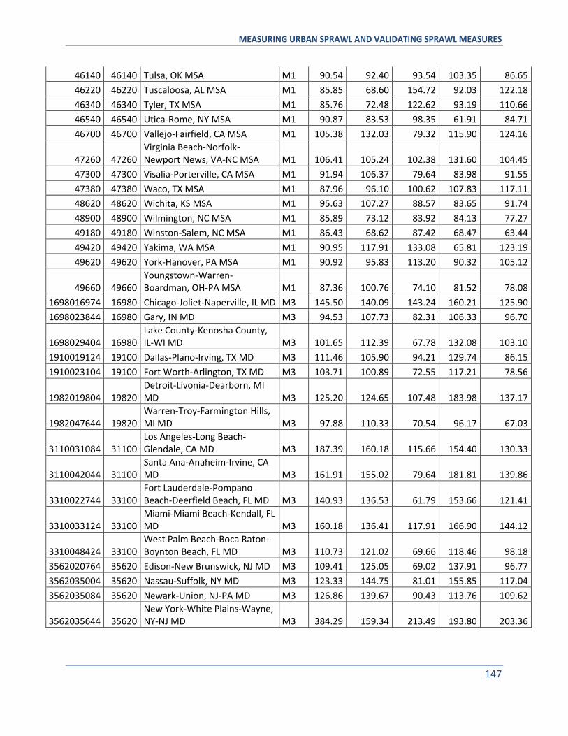
MEASURING URBAN SPRAWL AND VALIDATING SPRAWL MEASURES
147
46140 46140 Tulsa, OK MSA M1 90.54 92.40 93.54 103.35 86.65
46220 46220 Tuscaloosa, AL MSA M1 85.85 68.60 154.72 92.03 122.18
46340 46340 Tyler, TX MSA M1 85.76 72.48 122.62 93.19 110.66
46540 46540 Utica-Rome, NY MSA M1 90.87 83.53 98.35 61.91 84.71
46700 46700 Vallejo-Fairfield, CA MSA M1 105.38 132.03 79.32 115.90 124.16
47260 47260 Virginia Beach-Norfolk-Newport News, VA-NC MSA M1 106.41 105.24 102.38 131.60 104.45
47300 47300 Visalia-Porterville, CA MSA M1 91.94 106.37 79.64 83.98 91.55
47380 47380 Waco, TX MSA M1 87.96 96.10 100.62 107.83 117.11
48620 48620 Wichita, KS MSA M1 95.63 107.27 88.57 83.65 91.74
48900 48900 Wilmington, NC MSA M1 85.89 73.12 83.92 84.13 77.27
49180 49180 Winston-Salem, NC MSA M1 86.43 68.62 87.42 68.47 63.44
49420 49420 Yakima, WA MSA M1 90.95 117.91 133.08 65.81 123.19
49620 49620 York-Hanover, PA MSA M1 90.92 95.83 113.20 90.32 105.12
49660 49660 Youngstown-Warren-Boardman, OH-PA MSA M1 87.36 100.76 74.10 81.52 78.08
1698016974 16980 Chicago-Joliet-Naperville, IL MD M3 145.50 140.09 143.24 160.21 125.90
1698023844 16980 Gary, IN MD M3 94.53 107.73 82.31 106.33 96.70
1698029404 16980 Lake County-Kenosha County, IL-WI MD M3 101.65 112.39 67.78 132.08 103.10
1910019124 19100 Dallas-Plano-Irving, TX MD M3 111.46 105.90 94.21 129.74 86.15
1910023104 19100 Fort Worth-Arlington, TX MD M3 103.71 100.89 72.55 117.21 78.56
1982019804 19820 Detroit-Livonia-Dearborn, MI MD M3 125.20 124.65 107.48 183.98 137.17
1982047644 19820 Warren-Troy-Farmington Hills, MI MD M3 97.88 110.33 70.54 96.17 67.03
3110031084 31100 Los Angeles-Long Beach-Glendale, CA MD M3 187.39 160.18 115.66 154.40 130.33
3110042044 31100 Santa Ana-Anaheim-Irvine, CA MD M3 161.91 155.02 79.64 181.81 139.86
3310022744 33100 Fort Lauderdale-Pompano Beach-Deerfield Beach, FL MD M3 140.93 136.53 61.79 153.66 121.41
3310033124 33100 Miami-Miami Beach-Kendall, FL MD M3 160.18 136.41 117.91 166.90 144.12
3310048424 33100 West Palm Beach-Boca Raton-Boynton Beach, FL MD M3 110.73 121.02 69.66 118.46 98.18
3562020764 35620 Edison-New Brunswick, NJ MD M3 109.41 125.05 69.02 137.91 96.77
3562035004 35620 Nassau-Suffolk, NY MD M3 123.33 144.75 81.01 155.85 117.04
3562035084 35620 Newark-Union, NJ-PA MD M3 126.86 139.67 90.43 113.76 109.62
3562035644 35620 New York-White Plains-Wayne, NY-NJ MD M3 384.29 159.34 213.49 193.80 203.36
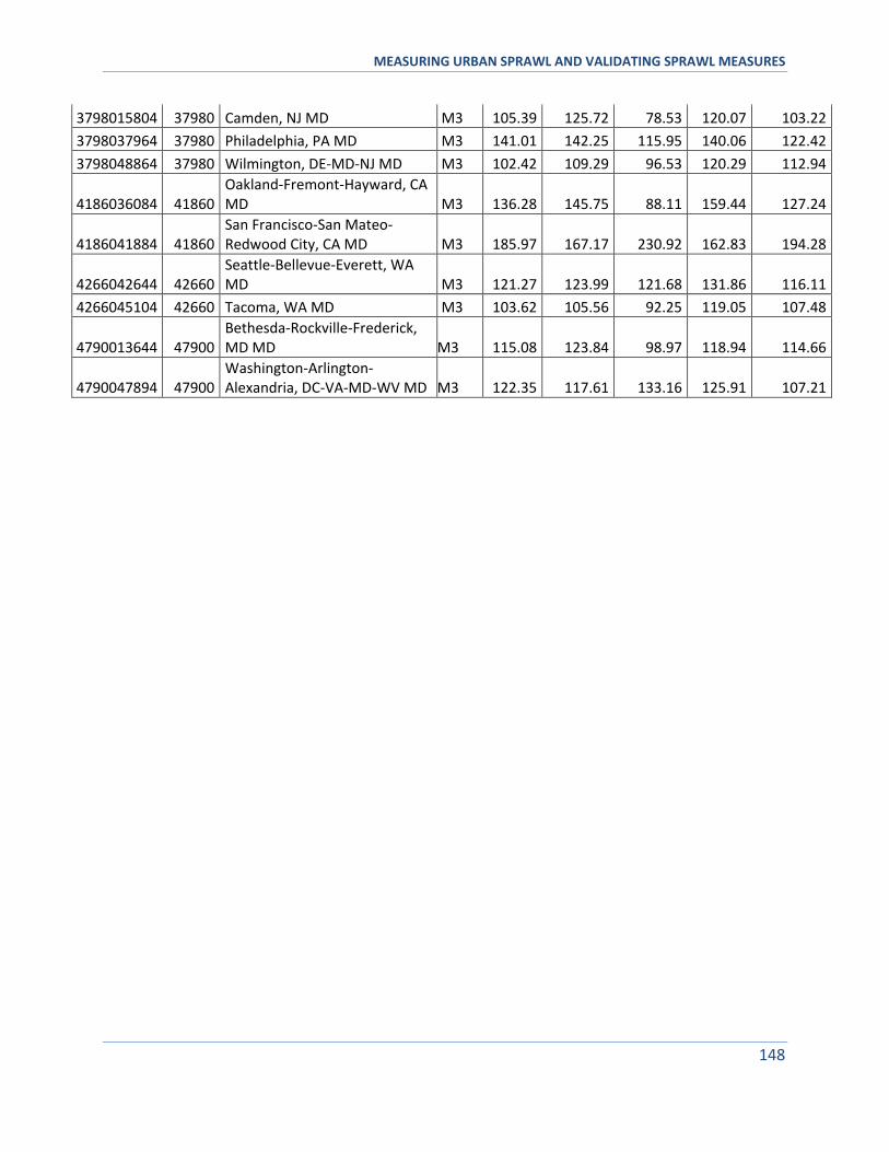
MEASURING URBAN SPRAWL AND VALIDATING SPRAWL MEASURES
148
3798015804 37980 Camden, NJ MD M3 105.39 125.72 78.53 120.07 103.22
3798037964 37980 Philadelphia, PA MD M3 141.01 142.25 115.95 140.06 122.42
3798048864 37980 Wilmington, DE-MD-NJ MD M3 102.42 109.29 96.53 120.29 112.94
4186036084 41860 Oakland-Fremont-Hayward, CA MD M3 136.28 145.75 88.11 159.44 127.24
4186041884 41860 San Francisco-San Mateo-Redwood City, CA MD M3 185.97 167.17 230.92 162.83 194.28
4266042644 42660 Seattle-Bellevue-Everett, WA MD M3 121.27 123.99 121.68 131.86 116.11
4266045104 42660 Tacoma, WA MD M3 103.62 105.56 92.25 119.05 107.48
4790013644 47900 Bethesda-Rockville-Frederick, MD MD M3 115.08 123.84 98.97 118.94 114.66
4790047894 47900 Washington-Arlington-Alexandria, DC-VA-MD-WV MD M3 122.35 117.61 133.16 125.91 107.21
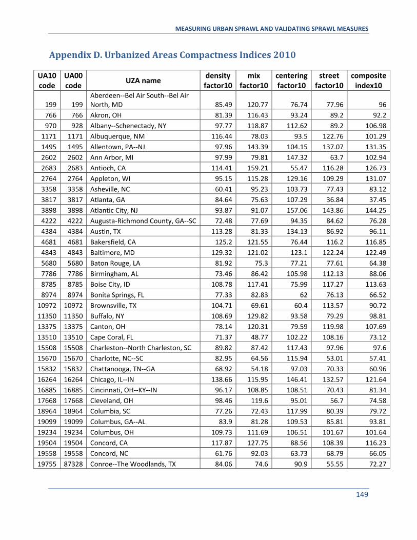
MEASURING URBAN SPRAWL AND VALIDATING SPRAWL MEASURES
149
Appendix D. Urbanized Areas Compactness Indices 2010
UA10 code
UA00 code
UZA name density factor10
mix factor10
centering factor10
street factor10
composite index10
199 199 Aberdeen--Bel Air South--Bel Air North, MD 85.49 120.77 76.74 77.96 96
766 766 Akron, OH 81.39 116.43 93.24 89.2 92.2
970 928 Albany--Schenectady, NY 97.77 118.87 112.62 89.2 106.98
1171 1171 Albuquerque, NM 116.44 78.03 93.5 122.76 101.29
1495 1495 Allentown, PA--NJ 97.96 143.39 104.15 137.07 131.35
2602 2602 Ann Arbor, MI 97.99 79.81 147.32 63.7 102.94
2683 2683 Antioch, CA 114.41 159.21 55.47 116.28 126.73
2764 2764 Appleton, WI 95.15 115.28 129.16 109.29 131.07
3358 3358 Asheville, NC 60.41 95.23 103.73 77.43 83.12
3817 3817 Atlanta, GA 84.64 75.63 107.29 36.84 37.45
3898 3898 Atlantic City, NJ 93.87 91.07 157.06 143.86 144.25
4222 4222 Augusta-Richmond County, GA--SC 72.48 77.69 94.35 84.62 76.28
4384 4384 Austin, TX 113.28 81.33 134.13 86.92 96.11
4681 4681 Bakersfield, CA 125.2 121.55 76.44 116.2 116.85
4843 4843 Baltimore, MD 129.32 121.02 123.1 122.24 122.49
5680 5680 Baton Rouge, LA 81.92 75.3 77.21 77.61 64.38
7786 7786 Birmingham, AL 73.46 86.42 105.98 112.13 88.06
8785 8785 Boise City, ID 108.78 117.41 75.99 117.27 113.63
8974 8974 Bonita Springs, FL 77.33 82.83 62 76.13 66.52
10972 10972 Brownsville, TX 104.71 69.61 60.4 113.57 90.72
11350 11350 Buffalo, NY 108.69 129.82 93.58 79.29 98.81
13375 13375 Canton, OH 78.14 120.31 79.59 119.98 107.69
13510 13510 Cape Coral, FL 71.37 48.77 102.22 108.16 73.12
15508 15508 Charleston--North Charleston, SC 89.82 87.42 117.43 97.96 97.6
15670 15670 Charlotte, NC--SC 82.95 64.56 115.94 53.01 57.41
15832 15832 Chattanooga, TN--GA 68.92 54.18 97.03 70.33 60.96
16264 16264 Chicago, IL--IN 138.66 115.95 146.41 132.57 121.64
16885 16885 Cincinnati, OH--KY--IN 96.17 108.85 108.51 70.43 81.34
17668 17668 Cleveland, OH 98.46 119.6 95.01 56.7 74.58
18964 18964 Columbia, SC 77.26 72.43 117.99 80.39 79.72
19099 19099 Columbus, GA--AL 83.9 81.28 109.53 85.81 93.81
19234 19234 Columbus, OH 109.73 111.69 106.51 101.67 101.64
19504 19504 Concord, CA 117.87 127.75 88.56 108.39 116.23
19558 19558 Concord, NC 61.76 92.03 63.73 68.79 66.05
19755 87328 Conroe--The Woodlands, TX 84.06 74.6 90.9 55.55 72.27
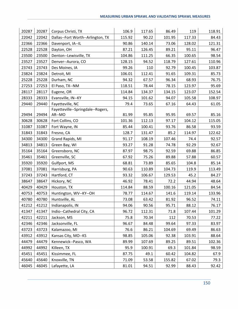
MEASURING URBAN SPRAWL AND VALIDATING SPRAWL MEASURES
150
20287 20287 Corpus Christi, TX 106.9 117.65 86.49 119 118.91
22042 22042 Dallas--Fort Worth--Arlington, TX 115.92 90.22 101.95 117.33 84.43
22366 22366 Davenport, IA--IL 90.86 140.14 73.06 128.02 121.31
22528 22528 Dayton, OH 87.21 126.45 89.21 95.11 96.47
23500 23500 Denton--Lewisville, TX 104.86 111.25 66.35 100.65 98.54
23527 23527 Denver--Aurora, CO 128.15 94.52 118.79 127.61 110.96
23743 23743 Des Moines, IA 99.26 110 92.79 100.45 103.87
23824 23824 Detroit, MI 106.01 112.41 91.65 109.31 85.73
25228 25228 Durham, NC 94.32 67.57 96.34 68.93 76.75
27253 27253 El Paso, TX--NM 118.51 78.44 78.15 123.97 95.69
28117 28117 Eugene, OR 114.84 134.37 134.15 123.07 152.54
28333 28333 Evansville, IN--KY 94.15 101.62 94.07 105.58 108.97
29440 29440 Fayetteville, NC 79.4 73.65 67.16 64.43 61.05
29494 29494 Fayetteville--Springdale--Rogers, AR--MO 81.99 95.85 95.95 69.57 85.16
30628 30628 Fort Collins, CO 101.36 112.13 97.17 104.12 115.05
31087 31087 Fort Wayne, IN 85.44 100.41 93.76 86.58 93.59
31843 31843 Fresno, CA 128.7 131.47 85.2 114.97 122.62
34300 34300 Grand Rapids, MI 91.17 108.19 107.46 74.4 92.57
34813 34813 Green Bay, WI 93.27 91.28 74.78 92.29 92.67
35164 35164 Greensboro, NC 87.97 98.75 92.59 69.88 86.85
35461 35461 Greenville, SC 67.92 75.26 89.88 57.88 60.57
35920 35920 Gulfport, MS 68.81 73.89 85.65 104.8 85.14
37081 37081 Harrisburg, PA 90.63 110.89 104.73 119.9 113.49
37243 37243 Hartford, CT 93.32 106.67 129.53 45.2 84.27
38647 38647 Hickory, NC 46.92 78.41 72.2 44.94 48.64
40429 40429 Houston, TX 114.84 88.59 100.16 121.05 84.54
40753 40753 Huntington, WV--KY--OH 78.77 114.67 141.6 119.14 133.96
40780 40780 Huntsville, AL 73.08 63.42 81.92 96.52 74.11
41212 41212 Indianapolis, IN 94.06 90.56 95.71 88.12 76.17
41347 41347 Indio--Cathedral City, CA 96.72 112.31 71.8 107.44 101.29
42211 42211 Jackson, MS 75.8 70.34 112 70.53 77.22
42346 42346 Jacksonville, FL 96.67 84.48 99.64 97.33 83.97
43723 43723 Kalamazoo, MI 76.6 86.21 104.69 69.49 86.63
43912 43912 Kansas City, MO--KS 98.85 105.06 92.38 103.91 88.64
44479 44479 Kennewick--Pasco, WA 89.99 107.69 89.25 89.51 102.36
44992 44992 Killeen, TX 95.9 100.91 69.3 101.84 98.59
45451 45451 Kissimmee, FL 87.75 49.1 60.42 104.82 67.9
45640 45640 Knoxville, TN 71.09 53.58 155.82 67.02 79.3
46045 46045 Lafayette, LA 81.01 94.51 92.99 88.43 92.42
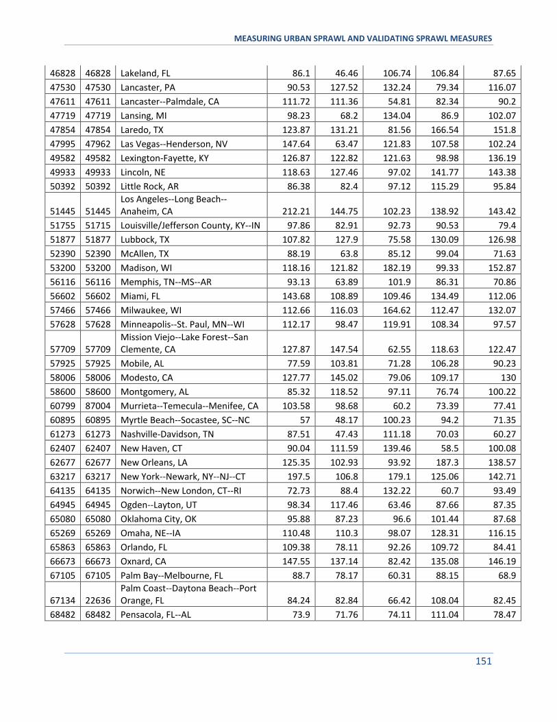
MEASURING URBAN SPRAWL AND VALIDATING SPRAWL MEASURES
151
46828 46828 Lakeland, FL 86.1 46.46 106.74 106.84 87.65
47530 47530 Lancaster, PA 90.53 127.52 132.24 79.34 116.07
47611 47611 Lancaster--Palmdale, CA 111.72 111.36 54.81 82.34 90.2
47719 47719 Lansing, MI 98.23 68.2 134.04 86.9 102.07
47854 47854 Laredo, TX 123.87 131.21 81.56 166.54 151.8
47995 47962 Las Vegas--Henderson, NV 147.64 63.47 121.83 107.58 102.24
49582 49582 Lexington-Fayette, KY 126.87 122.82 121.63 98.98 136.19
49933 49933 Lincoln, NE 118.63 127.46 97.02 141.77 143.38
50392 50392 Little Rock, AR 86.38 82.4 97.12 115.29 95.84
51445 51445 Los Angeles--Long Beach--Anaheim, CA 212.21 144.75 102.23 138.92 143.42
51755 51715 Louisville/Jefferson County, KY--IN 97.86 82.91 92.73 90.53 79.4
51877 51877 Lubbock, TX 107.82 127.9 75.58 130.09 126.98
52390 52390 McAllen, TX 88.19 63.8 85.12 99.04 71.63
53200 53200 Madison, WI 118.16 121.82 182.19 99.33 152.87
56116 56116 Memphis, TN--MS--AR 93.13 63.89 101.9 86.31 70.86
56602 56602 Miami, FL 143.68 108.89 109.46 134.49 112.06
57466 57466 Milwaukee, WI 112.66 116.03 164.62 112.47 132.07
57628 57628 Minneapolis--St. Paul, MN--WI 112.17 98.47 119.91 108.34 97.57
57709 57709 Mission Viejo--Lake Forest--San Clemente, CA 127.87 147.54 62.55 118.63 122.47
57925 57925 Mobile, AL 77.59 103.81 71.28 106.28 90.23
58006 58006 Modesto, CA 127.77 145.02 79.06 109.17 130
58600 58600 Montgomery, AL 85.32 118.52 97.11 76.74 100.22
60799 87004 Murrieta--Temecula--Menifee, CA 103.58 98.68 60.2 73.39 77.41
60895 60895 Myrtle Beach--Socastee, SC--NC 57 48.17 100.23 94.2 71.35
61273 61273 Nashville-Davidson, TN 87.51 47.43 111.18 70.03 60.27
62407 62407 New Haven, CT 90.04 111.59 139.46 58.5 100.08
62677 62677 New Orleans, LA 125.35 102.93 93.92 187.3 138.57
63217 63217 New York--Newark, NY--NJ--CT 197.5 106.8 179.1 125.06 142.71
64135 64135 Norwich--New London, CT--RI 72.73 88.4 132.22 60.7 93.49
64945 64945 Ogden--Layton, UT 98.34 117.46 63.46 87.66 87.35
65080 65080 Oklahoma City, OK 95.88 87.23 96.6 101.44 87.68
65269 65269 Omaha, NE--IA 110.48 110.3 98.07 128.31 116.15
65863 65863 Orlando, FL 109.38 78.11 92.26 109.72 84.41
66673 66673 Oxnard, CA 147.55 137.14 82.42 135.08 146.19
67105 67105 Palm Bay--Melbourne, FL 88.7 78.17 60.31 88.15 68.9
67134 22636 Palm Coast--Daytona Beach--Port Orange, FL 84.24 82.84 66.42 108.04 82.45
68482 68482 Pensacola, FL--AL 73.9 71.76 74.11 111.04 78.47

MEASURING URBAN SPRAWL AND VALIDATING SPRAWL MEASURES
152
68509 68509 Peoria, IL 85.82 104.21 125.17 113.45 120.49
69076 69076 Philadelphia, PA--NJ--DE--MD 127.16 124.32 131.46 105.73 109.05
69184 69184 Phoenix--Mesa, AZ 119.2 79.12 99.99 106.59 80.27
69697 69697 Pittsburgh, PA 93.7 119.21 125.55 117.1 109.25
71263 71263 Portland, ME 88.48 123.43 148.13 85.12 130.27
71317 71317 Portland, OR--WA 127.64 129.26 107.58 135.17 126.14
71479 71479 Port St. Lucie, FL 78.65 57.1 76.99 103.04 71.26
71803 71803 Poughkeepsie--Newburgh, NY--NJ 75.26 112.65 121.96 43.25 84.82
72559 72559 Provo--Orem, UT 113.81 130.08 77.33 100.13 110.6
73261 73261 Raleigh, NC 90.27 77.3 112.47 54.9 68.86
73693 73693 Reading, PA 127.71 150.87 124.45 147.46 169.32
74179 74179 Reno, NV--CA 101.13 59.47 123.12 94.24 95.67
74746 74746 Richmond, VA 94.09 83.03 111.23 109.31 93.1
75340 75340 Riverside--San Bernardino, CA 119.16 112.94 81.81 82.29 84.2
75421 75421 Roanoke, VA 83.87 108.45 81.82 110.57 105.72
75664 75664 Rochester, NY 103 101.93 103.14 61.44 85.12
75718 75718 Rockford, IL 86.89 103.05 96.03 119.57 109.98
76474 76474 Round Lake Beach--McHenry--Grayslake, IL--WI 80.35 83.85 79.57 90.59 81.75
77068 77068 Sacramento, CA 125.63 104.85 109.31 107.52 106.02
77770 77770 St. Louis, MO--IL 100.04 114.26 104.27 110.7 96.18
78229 78229 Salem, OR 115.59 125.71 112.5 103.81 133.51
78499 78499 Salt Lake City--West Valley City, UT 130.73 116.64 84.13 99.9 105.81
78580 78580 San Antonio, TX 113.62 85.4 92.02 104.86 85.2
78904 78904 San Francisco--Oakland, CA 205.69 129.92 164.34 153.38 180.94
79039 79039 San Jose, CA 181.13 136.26 86.67 127.03 139.98
79309 79309 Santa Clarita, CA 120.29 129.69 81.81 93.51 119.53
79606 79606 Sarasota--Bradenton, FL 84.4 94.94 93.16 115.72 93.95
79768 79768 Savannah, GA 82.3 96.52 110.11 111.85 109.61
80227 80227 Scranton, PA 95.52 145.27 102.54 133.3 135.5
80389 80389 Seattle, WA 118.83 89.41 142.43 110.09 104.65
81739 81739 Shreveport, LA 80.89 74.13 70.96 102.49 79.07
83116 83116 South Bend, IN--MI 79.42 91.31 105.6 129.25 110.77
83764 83764 Spokane, WA 97.43 109.36 103.98 141.33 125.49
83953 83953 Springfield, MO 86.57 110.76 68.49 115.03 101.06
85087 85087 Stockton, CA 126.41 131.34 98.73 117.22 134.67
86302 86302 Syracuse, NY 100.81 110.01 133.54 85.98 116.05
86464 86464 Tallahassee, FL 97.65 71.33 144.71 84.14 109.39
86599 86599 Tampa--St. Petersburg, FL 103.05 92.69 93.15 122.73 87.63
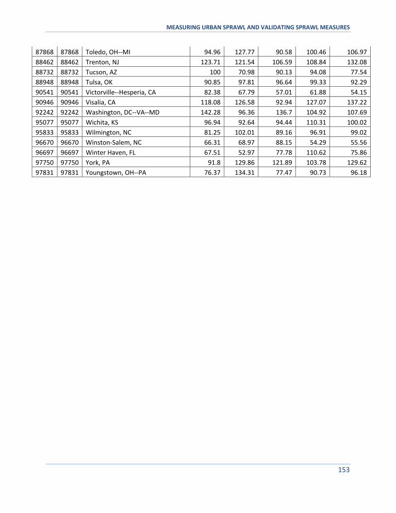
MEASURING URBAN SPRAWL AND VALIDATING SPRAWL MEASURES
153
87868 87868 Toledo, OH--MI 94.96 127.77 90.58 100.46 106.97
88462 88462 Trenton, NJ 123.71 121.54 106.59 108.84 132.08
88732 88732 Tucson, AZ 100 70.98 90.13 94.08 77.54
88948 88948 Tulsa, OK 90.85 97.81 96.64 99.33 92.29
90541 90541 Victorville--Hesperia, CA 82.38 67.79 57.01 61.88 54.15
90946 90946 Visalia, CA 118.08 126.58 92.94 127.07 137.22
92242 92242 Washington, DC--VA--MD 142.28 96.36 136.7 104.92 107.69
95077 95077 Wichita, KS 96.94 92.64 94.44 110.31 100.02
95833 95833 Wilmington, NC 81.25 102.01 89.16 96.91 99.02
96670 96670 Winston-Salem, NC 66.31 68.97 88.15 54.29 55.56
96697 96697 Winter Haven, FL 67.51 52.97 77.78 110.62 75.86
97750 97750 York, PA 91.8 129.86 121.89 103.78 129.62
97831 97831 Youngstown, OH--PA 76.37 134.31 77.47 90.73 96.18
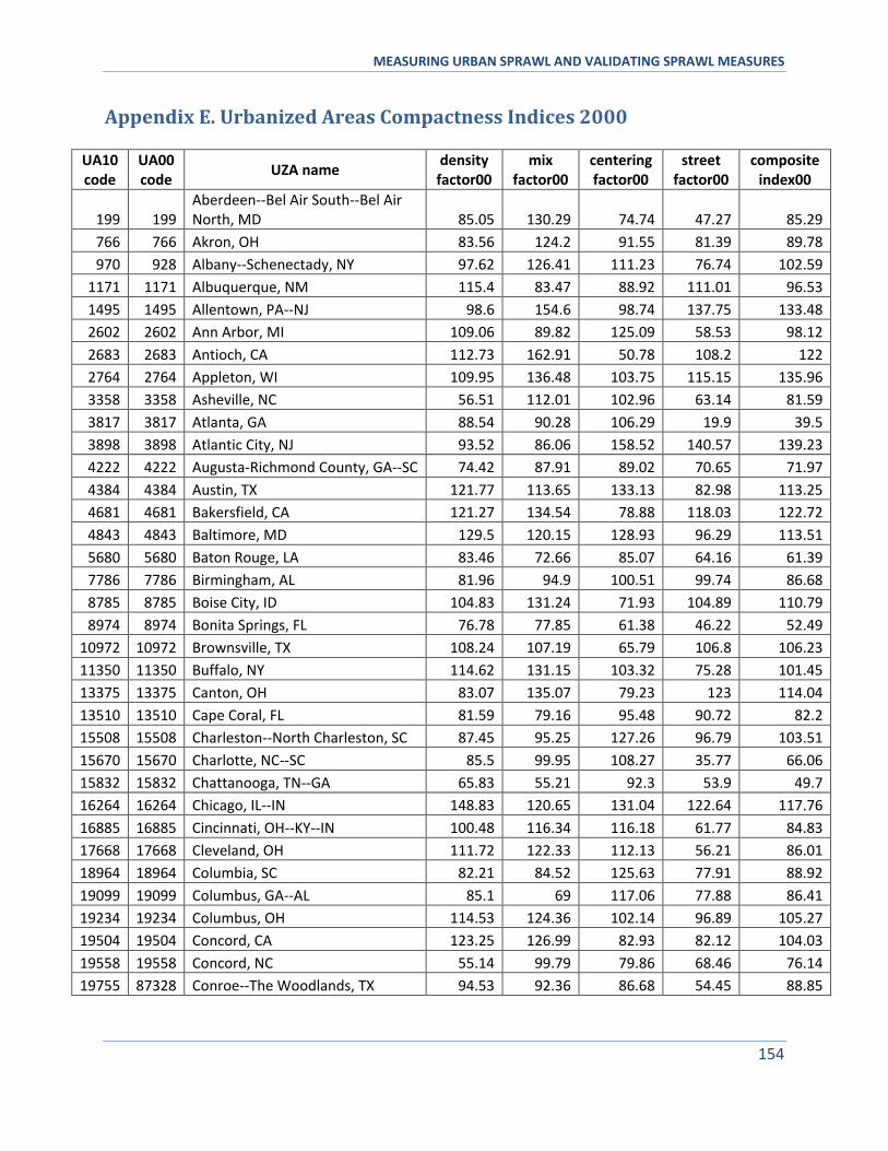
MEASURING URBAN SPRAWL AND VALIDATING SPRAWL MEASURES
154
Appendix E. Urbanized Areas Compactness Indices 2000
UA10 code
UA00 code
UZA name density factor00
mix factor00
centering factor00
street factor00
composite index00
199 199 Aberdeen--Bel Air South--Bel Air North, MD 85.05 130.29 74.74 47.27 85.29
766 766 Akron, OH 83.56 124.2 91.55 81.39 89.78
970 928 Albany--Schenectady, NY 97.62 126.41 111.23 76.74 102.59
1171 1171 Albuquerque, NM 115.4 83.47 88.92 111.01 96.53
1495 1495 Allentown, PA--NJ 98.6 154.6 98.74 137.75 133.48
2602 2602 Ann Arbor, MI 109.06 89.82 125.09 58.53 98.12
2683 2683 Antioch, CA 112.73 162.91 50.78 108.2 122
2764 2764 Appleton, WI 109.95 136.48 103.75 115.15 135.96
3358 3358 Asheville, NC 56.51 112.01 102.96 63.14 81.59
3817 3817 Atlanta, GA 88.54 90.28 106.29 19.9 39.5
3898 3898 Atlantic City, NJ 93.52 86.06 158.52 140.57 139.23
4222 4222 Augusta-Richmond County, GA--SC 74.42 87.91 89.02 70.65 71.97
4384 4384 Austin, TX 121.77 113.65 133.13 82.98 113.25
4681 4681 Bakersfield, CA 121.27 134.54 78.88 118.03 122.72
4843 4843 Baltimore, MD 129.5 120.15 128.93 96.29 113.51
5680 5680 Baton Rouge, LA 83.46 72.66 85.07 64.16 61.39
7786 7786 Birmingham, AL 81.96 94.9 100.51 99.74 86.68
8785 8785 Boise City, ID 104.83 131.24 71.93 104.89 110.79
8974 8974 Bonita Springs, FL 76.78 77.85 61.38 46.22 52.49
10972 10972 Brownsville, TX 108.24 107.19 65.79 106.8 106.23
11350 11350 Buffalo, NY 114.62 131.15 103.32 75.28 101.45
13375 13375 Canton, OH 83.07 135.07 79.23 123 114.04
13510 13510 Cape Coral, FL 81.59 79.16 95.48 90.72 82.2
15508 15508 Charleston--North Charleston, SC 87.45 95.25 127.26 96.79 103.51
15670 15670 Charlotte, NC--SC 85.5 99.95 108.27 35.77 66.06
15832 15832 Chattanooga, TN--GA 65.83 55.21 92.3 53.9 49.7
16264 16264 Chicago, IL--IN 148.83 120.65 131.04 122.64 117.76
16885 16885 Cincinnati, OH--KY--IN 100.48 116.34 116.18 61.77 84.83
17668 17668 Cleveland, OH 111.72 122.33 112.13 56.21 86.01
18964 18964 Columbia, SC 82.21 84.52 125.63 77.91 88.92
19099 19099 Columbus, GA--AL 85.1 69 117.06 77.88 86.41
19234 19234 Columbus, OH 114.53 124.36 102.14 96.89 105.27
19504 19504 Concord, CA 123.25 126.99 82.93 82.12 104.03
19558 19558 Concord, NC 55.14 99.79 79.86 68.46 76.14
19755 87328 Conroe--The Woodlands, TX 94.53 92.36 86.68 54.45 88.85
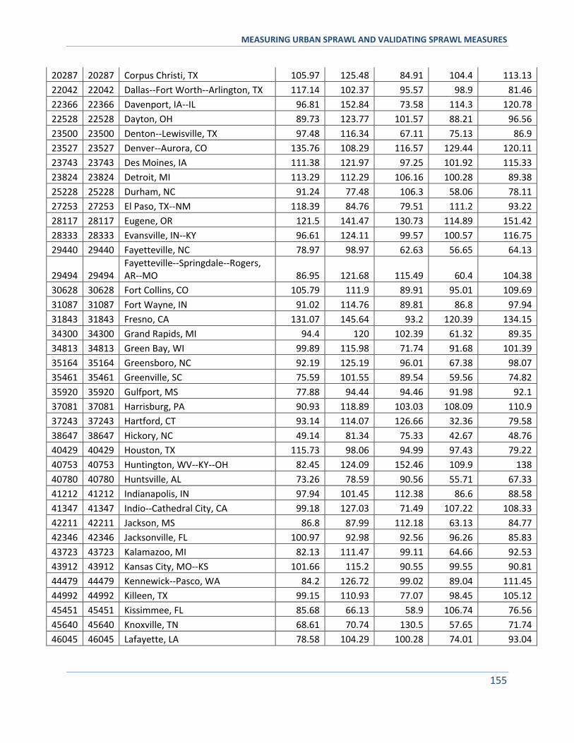
MEASURING URBAN SPRAWL AND VALIDATING SPRAWL MEASURES
155
20287 20287 Corpus Christi, TX 105.97 125.48 84.91 104.4 113.13
22042 22042 Dallas--Fort Worth--Arlington, TX 117.14 102.37 95.57 98.9 81.46
22366 22366 Davenport, IA--IL 96.81 152.84 73.58 114.3 120.78
22528 22528 Dayton, OH 89.73 123.77 101.57 88.21 96.56
23500 23500 Denton--Lewisville, TX 97.48 116.34 67.11 75.13 86.9
23527 23527 Denver--Aurora, CO 135.76 108.29 116.57 129.44 120.11
23743 23743 Des Moines, IA 111.38 121.97 97.25 101.92 115.33
23824 23824 Detroit, MI 113.29 112.29 106.16 100.28 89.38
25228 25228 Durham, NC 91.24 77.48 106.3 58.06 78.11
27253 27253 El Paso, TX--NM 118.39 84.76 79.51 111.2 93.22
28117 28117 Eugene, OR 121.5 141.47 130.73 114.89 151.42
28333 28333 Evansville, IN--KY 96.61 124.11 99.57 100.57 116.75
29440 29440 Fayetteville, NC 78.97 98.97 62.63 56.65 64.13
29494 29494 Fayetteville--Springdale--Rogers, AR--MO 86.95 121.68 115.49 60.4 104.38
30628 30628 Fort Collins, CO 105.79 111.9 89.91 95.01 109.69
31087 31087 Fort Wayne, IN 91.02 114.76 89.81 86.8 97.94
31843 31843 Fresno, CA 131.07 145.64 93.2 120.39 134.15
34300 34300 Grand Rapids, MI 94.4 120 102.39 61.32 89.35
34813 34813 Green Bay, WI 99.89 115.98 71.74 91.68 101.39
35164 35164 Greensboro, NC 92.19 125.19 96.01 67.38 98.07
35461 35461 Greenville, SC 75.59 101.55 89.54 59.56 74.82
35920 35920 Gulfport, MS 77.88 94.44 94.46 91.98 92.1
37081 37081 Harrisburg, PA 90.93 118.89 103.03 108.09 110.9
37243 37243 Hartford, CT 93.14 114.07 126.66 32.36 79.58
38647 38647 Hickory, NC 49.14 81.34 75.33 42.67 48.76
40429 40429 Houston, TX 115.73 98.06 94.99 97.43 79.22
40753 40753 Huntington, WV--KY--OH 82.45 124.09 152.46 109.9 138
40780 40780 Huntsville, AL 73.26 78.59 90.56 55.71 67.33
41212 41212 Indianapolis, IN 97.94 101.45 112.38 86.6 88.58
41347 41347 Indio--Cathedral City, CA 99.18 127.03 71.49 107.22 108.33
42211 42211 Jackson, MS 86.8 87.99 112.18 63.13 84.77
42346 42346 Jacksonville, FL 100.97 92.98 92.56 96.26 85.83
43723 43723 Kalamazoo, MI 82.13 111.47 99.11 64.66 92.53
43912 43912 Kansas City, MO--KS 101.66 115.2 90.55 99.55 90.81
44479 44479 Kennewick--Pasco, WA 84.2 126.72 99.02 89.04 111.45
44992 44992 Killeen, TX 99.15 110.93 77.07 98.45 105.12
45451 45451 Kissimmee, FL 85.68 66.13 58.9 106.74 76.56
45640 45640 Knoxville, TN 68.61 70.74 130.5 57.65 71.74
46045 46045 Lafayette, LA 78.58 104.29 100.28 74.01 93.04
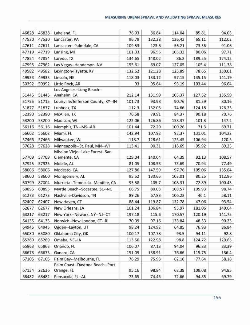
MEASURING URBAN SPRAWL AND VALIDATING SPRAWL MEASURES
156
46828 46828 Lakeland, FL 76.03 86.84 114.04 85.81 94.03
47530 47530 Lancaster, PA 96.79 132.28 126.42 65.11 112.02
47611 47611 Lancaster--Palmdale, CA 109.53 123.6 56.21 73.56 91.06
47719 47719 Lansing, MI 101.03 96.55 105.33 80.06 97.71
47854 47854 Laredo, TX 134.65 148.02 86.2 189.55 174.12
47995 47962 Las Vegas--Henderson, NV 155.61 69.07 127.05 105.4 111.38
49582 49582 Lexington-Fayette, KY 132.62 121.28 125.89 78.65 130.01
49933 49933 Lincoln, NE 118.03 133.12 97.15 135.15 141.19
50392 50392 Little Rock, AR 93 95.64 93.19 103.44 96.64
51445 51445 Los Angeles--Long Beach--Anaheim, CA 212.14 131.99 105.37 127.52 135.59
51755 51715 Louisville/Jefferson County, KY--IN 101.73 93.98 90.76 81.59 80.16
51877 51877 Lubbock, TX 112.3 132.03 74.66 124.18 126.23
52390 52390 McAllen, TX 76.58 79.91 84.37 90.18 70.76
53200 53200 Madison, WI 122.06 126.86 158.37 101.3 147.2
56116 56116 Memphis, TN--MS--AR 101.44 72.29 100.26 71.3 69.71
56602 56602 Miami, FL 142.94 107.92 93.37 131.01 104.22
57466 57466 Milwaukee, WI 118.7 128.61 125.45 106.94 120.5
57628 57628 Minneapolis--St. Paul, MN--WI 113.41 90.31 118.69 95.92 89.25
57709 57709 Mission Viejo--Lake Forest--San Clemente, CA 129.04 140.04 64.39 92.13 108.57
57925 57925 Mobile, AL 81.05 108.53 73.69 70.94 77.49
58006 58006 Modesto, CA 127.86 147.59 97.76 105.06 135.64
58600 58600 Montgomery, AL 95.52 130.65 103.01 80.25 112.96
60799 87004 Murrieta--Temecula--Menifee, CA 95.58 105.7 108.31 72.89 100.43
60895 60895 Myrtle Beach--Socastee, SC--NC 66.75 80.03 108.57 105.93 98.74
61273 61273 Nashville-Davidson, TN 89.26 67.83 106.22 46.1 58.11
62407 62407 New Haven, CT 88.44 119.87 132.78 47.06 93.54
62677 62677 New Orleans, LA 161.24 106.84 95.97 181.06 149.64
63217 63217 New York--Newark, NY--NJ--CT 197.18 115.6 170.57 120.19 141.75
64135 64135 Norwich--New London, CT--RI 70.09 97.16 133.84 48.33 90.23
64945 64945 Ogden--Layton, UT 98.24 124.92 64.85 76.93 86.84
65080 65080 Oklahoma City, OK 100.17 107.78 93.5 94.11 92.8
65269 65269 Omaha, NE--IA 113.56 122.98 98.8 124.72 120.65
65863 65863 Orlando, FL 106.07 87.13 94.04 96.83 83.39
66673 66673 Oxnard, CA 151.09 138.91 76.66 115.75 136.4
67105 67105 Palm Bay--Melbourne, FL 76.29 75.93 62.16 77.64 58.18
67134 22636 Palm Coast--Daytona Beach--Port Orange, FL 95.16 98.84 68.39 109.08 94.85
68482 68482 Pensacola, FL--AL 73.65 74.45 72.66 94.85 69.79
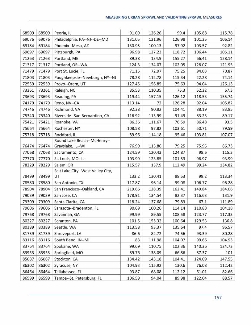
MEASURING URBAN SPRAWL AND VALIDATING SPRAWL MEASURES
157
68509 68509 Peoria, IL 91.09 126.26 99.4 105.88 115.78
69076 69076 Philadelphia, PA--NJ--DE--MD 131.05 121.96 126.98 101.25 106.14
69184 69184 Phoenix--Mesa, AZ 130.95 100.13 97.92 103.57 92.82
69697 69697 Pittsburgh, PA 96.98 127.23 118.72 106.44 105.11
71263 71263 Portland, ME 89.38 134.9 155.27 66.41 128.14
71317 71317 Portland, OR--WA 124.3 134.07 102.05 128.07 121.95
71479 71479 Port St. Lucie, FL 71.15 72.97 75.25 94.03 70.87
71803 71803 Poughkeepsie--Newburgh, NY--NJ 78.28 112.78 115.34 22.28 74.14
72559 72559 Provo--Orem, UT 127.45 156.85 75.63 94.04 126.13
73261 73261 Raleigh, NC 85.53 110.35 75.3 52.22 67.3
73693 73693 Reading, PA 119.44 157.15 126.12 118.53 155.74
74179 74179 Reno, NV--CA 113.14 72 126.28 92.04 105.82
74746 74746 Richmond, VA 92.38 90.82 104.41 88.19 83.85
75340 75340 Riverside--San Bernardino, CA 116.92 113.99 91.49 83.23 89.17
75421 75421 Roanoke, VA 86.36 111.67 76.59 86.48 93.5
75664 75664 Rochester, NY 108.58 97.82 103.61 50.71 79.59
75718 75718 Rockford, IL 89.96 114.18 95.46 103.81 107.07
76474 76474 Round Lake Beach--McHenry--Grayslake, IL--WI 76.99 115.86 79.25 75.95 86.73
77068 77068 Sacramento, CA 124.59 120.43 124.87 98.6 115.3
77770 77770 St. Louis, MO--IL 103.99 123.85 101.53 96.97 93.99
78229 78229 Salem, OR 115.57 137.9 112.49 99.24 134.82
78499 78499 Salt Lake City--West Valley City, UT 133.2 130.41 88.53 99.2 113.34
78580 78580 San Antonio, TX 117.87 96.14 99.08 106.77 96.28
78904 78904 San Francisco--Oakland, CA 219.66 128.39 162.41 149.84 184.06
79039 79039 San Jose, CA 178.91 134.54 82.37 116.63 131.9
79309 79309 Santa Clarita, CA 118.24 137.68 79.83 67.1 111.89
79606 79606 Sarasota--Bradenton, FL 90.69 100.26 114.14 110.88 104.18
79768 79768 Savannah, GA 99.99 89.55 108.58 123.77 117.33
80227 80227 Scranton, PA 101.5 155.32 100.64 129.53 136.8
80389 80389 Seattle, WA 113.58 93.37 135.64 97.4 96.57
81739 81739 Shreveport, LA 86.6 82.72 74.56 93.39 80.28
83116 83116 South Bend, IN--MI 83 111.98 104.07 99.66 104.93
83764 83764 Spokane, WA 99.69 110.75 102.36 140.36 124.73
83953 83953 Springfield, MO 89.76 138.09 66.86 87.37 101
85087 85087 Stockton, CA 134.42 145.18 104.41 124.09 147.55
86302 86302 Syracuse, NY 104.93 115.92 130.6 76.08 112.42
86464 86464 Tallahassee, FL 93.87 68.08 112.12 61.01 82.66
86599 86599 Tampa--St. Petersburg, FL 106.59 94.04 89.98 122.04 88.57
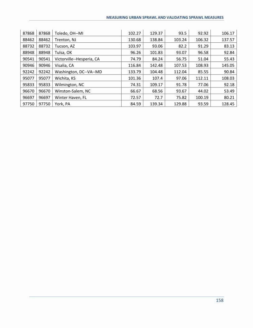
MEASURING URBAN SPRAWL AND VALIDATING SPRAWL MEASURES
158
87868 87868 Toledo, OH--MI 102.27 129.37 93.5 92.92 106.17
88462 88462 Trenton, NJ 130.68 138.84 103.24 106.32 137.57
88732 88732 Tucson, AZ 103.97 93.06 82.2 91.29 83.13
88948 88948 Tulsa, OK 96.26 101.83 93.07 96.58 92.84
90541 90541 Victorville--Hesperia, CA 74.79 84.24 56.75 51.04 55.43
90946 90946 Visalia, CA 116.84 142.48 107.53 108.93 145.05
92242 92242 Washington, DC--VA--MD 133.79 104.48 112.04 85.55 90.84
95077 95077 Wichita, KS 101.36 107.4 97.06 112.11 108.03
95833 95833 Wilmington, NC 74.31 109.17 91.78 77.06 92.18
96670 96670 Winston-Salem, NC 66.67 68.56 93.67 44.02 53.49
96697 96697 Winter Haven, FL 72.57 72.7 75.82 100.19 80.21
97750 97750 York, PA 84.59 139.34 129.88 93.59 128.45