Measuring the Stringency of Land-Use Regulation: The Case

of China’s Building-Height Limits

Jan K. Brueckner, Shihe Fu, Yizhen Gu and Junfu Zhang∗

March 23, 2016

Abstract

This paper develops a new approach for measuring the stringency of a major form

of land-use regulation, building-height restrictions, and it applies the method to an

extraordinary dataset of land-lease transactions from China. Our theory shows that

the elasticity of land price with respect to the floor-area ratio (FAR), an indicator of

the allowed building height for the parcel, is a measure of the regulation’s stringency

(the extent to which FAR is kept below the free-market level). Using a national sample,

estimation that allows this elasticity to be city-specific shows substantial variation in

the stringency of FAR regulation across Chinese cities, and additional evidence suggests

that stringency depends on certain city characteristics in a predictable fashion. Single-

city estimation for the large Beijing subsample, where site characteristics can be added

to the regression, indicates that the stringency of FAR regulation varies with certain site

characteristics, again in a predictable way (being high near the Tiananmen historical

sites). Further results using a different dataset show that FAR limits in Beijing are

adjusted in reponse to demand forces created by new subway stops.

Keywords: Floor-area ratio, density restriction, urban development, China.

JEL Classification: R14, R52.

∗Brueckner is a professor of economics at UC Irvine (E-mail: jkbrueck@uci.edu). Fu is a professor ofeconomics at Southwestern University of Finance and Economics (E-mail: fush@swufe.edu.cn). Gu is anassistant professor of economics at the Institute of Economic and Social Research at Jinan University (E-mail: yizhengu@gmail.com). Zhang is an associate professor of economics at Clark University (E-mail:juzhang@clarku.edu). We thank Paul Cheshire, Jeffrey Cohen, Gilles Duranton, Yuming Fu, Steve Ross,Xin Zhang, and audiences at the University of Connecticut, USC, University of Nevada-Las Vegas, the 2015Urban Economics Association Conference, the 2015 ASSA Annual Meetings, and the CES North Americanconference at Purdue University for their comments and suggestions.

1

1 Introduction

Land-use regulation has been a long-time focus of research by economists and other scholars.

Regulations are imposed in virtually every country in the world and take a variety of

forms. They include traditional zoning laws, which are designed to allocate land to different

uses while spatially separating them; restrictions on the density of development, which

range from building-height limits to minimum lot-size requirements to street set-back rules;

and restrictions on the volume of development, which include urban growth boundaries

that limit the land area available for development and annual caps on building permits.

Empirical research on land-use regulation has mainly focused on its impact on the prices

of both housing and land, although a few studies measure its effect on the rate of new

construction (see Gyourko and Molloy (2014) for an up-to-date survey). The evidence

shows that regulations tend to raise housing prices, a consequence of their tendency to

restrict housing supply, an effect that is separately documented in other studies.

The fact that regulations have price effects indicates that they are binding on devel-

opment decisions. While this is an important finding, the literature to date contains few

attempts to measure the stringency of land-use regulations, namely, the extent to which

they cause development decisions to diverge from free-market outcomes. For example, highly

stringent density restrictions would reduce development density far below the unregulated

level, while less-stringent regulations would have a milder effect. A highly stringent urban

growth boundary would constrain a city’s footprint to be much smaller than its free-market

size, while a less-stringent one would leave the footprint almost unaffected. Stringent zoning

regulations could seriously skew a city’s division of land between residential and commercial

uses away from a free-market division.

One line of work that provides a measure of regulatory stringency was originated by

Glaeser et al. (2005). They compare the marginal value of floor space estimated from an

hedonic model to construction cost per square foot for residential buildings in Manhattan,

with the gap (denoted the “regulatory tax”) being an index of the extent to which regula-

tions restrict development density below market levels.1 The present paper develops and

applies a distinctly different method for evaluating the stringency of land-use regulation.

The method is developed theoretically, and it is then applied to an extraordinary dataset

of land-lease transactions in China. We focus on the regulated floor-area ratio (FAR) for

leased parcels, which limits the ratio of the floor area within the proposed building to the

parcel’s lot size. Although FAR is affected by the amount of open space left on the lot,

it is effectively a measure of the allowed building height. A stringent FAR limit will thus

constrain the building height to be much lower than the one the developer would choose

in the absence of regulation. The unconstrained FAR is, of course, unobservable in the

presence of the regulation, which means that the stringency of FAR limit cannot be gauged

1Further references to related work can be found in Gyourko and Molloy (2014).

2

directly. However, we demonstrate theoretically that the stringency of the limit can be

inferred from the connection between land prices for leased parcels (which are available in

the data) and their FAR limits, and we then use this connection to evaluate the stringency

of FAR regulation in Chinese cities.

Because FAR regulation reduces the profitability of development, it reduces the devel-

oper’s willingness-to-pay for the land and thus its value. Accordingly, a higher allowed FAR,

by loosening the constraint on development, will raise the land price for the parcel. But

our theory shows that a more-precise conclusion can be derived. We show that the elastic-

ity of land price with respect to the FAR limit depends on the ratio of the unconstrained

and regulated FAR levels. In particular, this elasticity is large when that ratio is large, or

when the unconstrained FAR is high relative to the regulated FAR. Thus, relaxing a highly

stringent FAR limit (one with a high ratio) leads to a greater percentage increase in land

price than relaxing a less-stringent limit, an intuitively sensible conclusion.

We exploit this result using a land-lease dataset that consists of over 50,000 transactions

across more than 200 cities during the 2002-2011 period. Our results allow us to gauge the

restrictiveness of FAR regulation in China. We view FAR restrictiveness as being city-

specific, running a land-value regression using lease transactions from all cities but allowing

each city to have a different elasticity of individual parcel values with respect to parcel-

specific FAR limits. The estimated elasticity coefficients then tell us which Chinese cities

are most restrictive in their regulation of FAR. Under a second approach, we focus on a single

large city (Beijing), allowing the land-price/FAR elasticity (and thus FAR restrictiveness)

to vary according to site characteristics such as distance from the historic city center.

In a companion regression to the first exercise, we relates the restrictiveness of FAR at

the city level (as captured by city-specific coefficients in the land-price regression) to city

characteristics. Finally, using a different dataset for Beijing that shows FAR limits for

existing properties rather than new leases, we explore the factors that cause regulated FAR

levels to change over time.

While our method could be applied to land-value/FAR data from any country, China’s

rapid urban growth generates an ideal dataset, with a large volume of transactions and

considerable regulatory detail. Beyond its methodological contribution, the paper’s focus

on China helps to overcome a shortage of information about land-use regulation in one of the

world’s fastest growing economies. Only two rigorous studies (to the best of our knowledge)

have previously investigated China’s FAR restrictions. Fu and Somerville (2001) develop a

theoretical model and then show empirically that restricted FAR values deviate from the

developer’s optimal value in a way that reflects the local government’s goals. In a more

recent paper, Cai, Wang, and Zhang (2016) investigate abrogations of FAR restrictions in

China as a result of corruption. Using a unique dataset, they find that FAR is higher for

transactions that involve corruption and that corruption is more likely to influence on FAR

3

for parcels in desirable locations.2

The plan of the paper is as follows. Section 2 provides an overview of the institutional

setting in which land-lease transactions occur. Section 3 presents the theoretical model

and discusses empirical implementation. Section 4 discusses the determinants of regulated

FAR levels. Section 5 describes the national dataset and presents the results of the intercity

regressions. Section 6 presents the regression results using the Beijing portion of the national

data and then presents regressions using the separate Beijing dataset on FAR values for

existing properties. Section 7 offers conclusions.

2 Institutional Background

China is experiencing rapid urbanization, with the share of the urbanized population rising

from 21 percent in 1982 to over 50 percent today. This fast urban population growth

has been accommodated by an unprecedented spatial expansion of the country’s urbanized

areas. In 1982, China’s built-up urbanized area was 7,438 square kilometers. By 2011, it

had risen to 43,603 square kilometers.3

This explosive urbanization was fueled by rapid conversion of land from rural to urban

use, a process facilitated by local governments. By Chinese law, urban land is owned by the

state, and rural land is owned by local economic collectives. To facilitate urban expansion,

local governments acquire land from farmers at the urban fringe, paying compensation that

is often substantially below market value (Ding 2007, Hui et al. 2013). The local govern-

ments then transfer land-use rights to independent developers via a leasehold, generating

revenue that can be used for public investment and other purposes.4 In earlier years, lease

payments were decided through negotiations between land developers and government of-

ficials, which were conducive to corruption. Since 2004, local governments have used land

auctions to make the transactions of land-use rights more transparent. The maximum term

of the land lease is 70 years for residential uses, 50 years for industrial uses, and 40 years

for commercial uses.5

A local government’s land-use plan stipulates how a developer can use the leased land.

The plan usually specifies the usage type, indicating whether the land is for residential,

commercial, or industrial development, and it contains density restrictions, including the

FAR, green coverage, and sometimes a separate explicit height limit. In other countries

2A few related studies examine FAR regulation in other countries. Using data on 273 land lots in theTokyo area, Gao et al. (2006) estimate hedonic regressions to explore the effect of FAR restrictions on landprices. Brueckner and Sridhar (2012) measure welfare gains from relaxation of FAR restrictions in India.Barr and Cohen (2014) describe the FAR gradient and its evolution in New York City.

3See Ministry of Housing and Urban-Rural Development (2012) and National Bureau of Statistics ofChina (1983, 2012).

4Following a major tax reform in 1994, which weakened the tax base for local governments, local govern-ment officials learned that selling land-use rights is an effective way to generate revenue (Cao et al. 2008).In recent years, around 50 percent of local government revenue has come from land leases (Liu et al. 2012).

5When different branches of the government need land for construction of public infrastructure or militaryfacilities, land-use rights can be obtained through a direct allocation.

4

such as the United States, land-use regulations also restrict development density, but these

restrictions typically apply to many land parcels in a large section of a city. The unique

characteristic of urban planning in China is that controls and restrictions are designed and

implemented at the land parcel level. For our study, this unique institutional arrange-

ment allows us to study FAR restrictions at the land parcel level, both theoretically and

empirically.

As will be seen shortly, a local government interested in maximizing revenue from land

leases would impose no land-use restrictions at all, recognizing that unrestricted profit-

maximization on the part of developers leads to the highest land price. FAR restrictions

will be desirable, however, once it is recognized that the high densities associated with high

FARs impose costs on the local government, including the cost of providing supporting

infrastructure to the newly built community. As a result, local officials will not allow devel-

opers to set an unrestricted, profit-maximizing FAR, which would maximize land revenue,

but will instead sacrifice revenue by restricting the allowable FAR, with the goal of limiting

the infrastructure costs associated with higher densities.6 In this sense, local officials behave

as net revenue maximizers, taking the public costs associated with land development into

account.7 The resulting restrictions then generate an association between land price for a

site and its FAR limit, and by studying the strength of this association, we can infer the

restrictiveness of the limit.

3 Measuring FAR stringency

3.1 Theory

To explore the connection between land price and FAR, consider the standard urban land-

use model, as in Brueckner (1987). While this model is static, ignoring the long-lived

nature of housing, the following analysis can be adapted easily to the case where a housing

investment earns revenue over an extended period, as in Arnott and Lewis (1979). Let r

denote the land price per acre and p denote the price per square foot of housing, which

depends on a vector Z of locational attributes, including distance to the CBD, that affect

the attractiveness of the site (thus, p = p(Z)). Let h(S) denote square feet of housing

output per acre as a function of structural density S, which equals housing capital per acre

(h is concave, satisfying h′ > 0 and h′′ < 0). The housing developer’s profit per acre is

6It is a well-known theoretical point that FAR and other housing density restrictions can be explainedby invoking population-density externalities. See, for example, Bertaud and Brueckner (2005), Joshi andKono (2009), Kono and Joshi (2012), Kono et al. (2010), Mills (2005), Pines and Kono (2012), and Wheaton(1998).

7Lichtenberg and Ding (2009) have similarly treated local government officials in China as rational decisionmakers in the context of land conversion for urban uses, and Zhang (2011) assumes local government officialsto be rational revenue maximizers in a study of inter-jurisdictional competition for FDI in China. Asshown by Li and Zhou (2005) and follow-up research, better economic performance increases a local leader’sprobability of being promoted and decreases the probability of his or her career termination.

5

given by

π = ph(S) − iS − r, (1)

where i is the cost per unit of capital. The first-order condition for choice of S in the

absence of an FAR limit is

ph′(S) = i, (2)

and the S satisfying (2) is denoted S∗. The land price is then given by the zero profit

condition:

r = ph(S∗) − iS∗. (3)

An FAR limit imposes a maximal value for h(S), denoted h, which in turn imposes a

maximal value of S. This value is denoted S, and it satisfies h(S) = h. The effect of S on

the land price r is considered first, with the link between r and h analyzed below. Faced

with the FAR limit, developers will set S = S, and the land price will be given by

r = ph(S) − iS. (4)

The derivative of land price with respect to S is

∂r

∂S= ph′(S) − i > 0, (5)

where the inequality follows because the FAR constraint is binding, with S restricted below

its optimal value. If the FAR limit is not binding, then it will have no effect on development

decisions and thus no effect on r. In addition, the land price will depend on the vector Z:

∂r

∂Z=∂p

∂Zh(S). (6)

A higher value of a favorable site characteristic j such as accessibility to employment, for

which ∂p/∂Zj > 0, will raise the land price.8

Consider the elasticity of land price with respect to S, which is given by

Er,S ≡ ∂r

∂S

S

r=

[ph′(S) − i]S

ph(S) − iS. (7)

Since concavity of h means that h′(S)S < h(S), Er,S in (7) is less than unity, so that the

elasticity of land value with respect to a binding S limit is less than one.

To get additional information, ph′(S∗) = i can be used to eliminate i in (7). Doing so,

8An equivalent, but less familiar, modeling approach treats h rather than S as the choice variable, makinguse of a convext cost function c(h) (profit per acre is then ph− c(h) − r).

6

the expression becomes

Er,S =

[ph′

(S)− ph′ (S∗)

]S

ph(S)− ph′ (S∗)S

=

[h′(S)− h′ (S∗)

]S

h(S)− h′ (S∗)S

, (8)

showing that Er,S depends on S∗ as well as S (note that p cancels). At this point, it is

useful to impose a standard functional form for h. If h(S) = Sβ, with β < 1, then (8)

becomes

Er,S =

[βS

β−1 − β (S∗)β−1]S

Sβ − β (S∗)β−1 S

=βS

β−1 − β (S∗)β−1

Sβ−1 − β (S∗)β−1

=(S∗/S)1−β − 11β (S∗/S)1−β − 1

. (9)

Thus, the elasticity of land price with respect to S depends on the ratio of the developer’s

optimal S (S∗) to the restricted level, S. Furthermore, differentiation of (9) shows that

∂Er,S

∂(S∗/S)> 0, (10)

so that the elasticity is large when the restricted S lies far below the optimal value (making

S∗/S large). In other words, the percentage increase in land price from relaxing a very tight

S limit is greater than the percentage increase from relaxing a looser limit, a conclusion

that matches intuition.

Since h(S) = h implies Sβ

= h under the chosen functional form, it follows that S =

h1/β

. Therefore, the elasticity of land price with respect to h, denoted Er,h, equals 1/β

times the elasticity with respect to S, so that

Er,h ≡ ∂r

∂h

h

r=

Er,Sβ

. (11)

Given (11), it follows that Er,h, like Er,S , is increasing in S∗/S:

∂Er,h

∂(S∗/S)> 0. (12)

Thus, the percentage increase in land price from relaxing a tight FAR limit is greater than

the increase from relaxing a loose one. Note that since both Er,S and β are less than 1, the

elasticity Er,h can be either larger or smaller than 1, in contrast to Er,S itself.

As seen below, the empirical model will generate an estimate of Er,h, which is denoted

θ. Treating θ as a known value and imposing a value for β, (9) can then be solved for

the ratio S/S∗, which then allows the ratio of the FARs to be computed. The solution is

h(S)/h(S∗) = [(1− θ)/(1− θ/β)]−β/(1−β). Therefore, using the estimated θ and a value for

β, the actual ratio of the regulated and free-market FARs can be derived.

While the possibility of bribery has apparently been reduced by adoption of an auction

7

format for the lease transactions, it may still be present in some cases (Cai et al., 2013). To

see how bribery affects the previous results, suppose the developer can raise the effective

S by the factor σ > 1 by paying a bribe equal to 1 − λ of his revenue. This bribe is paid

to an official different from the one who sets S, a decision explained below (the mayor,

for example, rather than the city planner). The effective FAR limit is then σS, while the

observed limit remains at S, and p is replaced by λp. It can be shown that, in the elasticity

formula (9), the 1’s in both numerator and denominator are replaced by σ1−β/λ > 1. While

this change affects the magnitude of the elasticity, it does not alter the central conclusion

from (12) that the elasticity Er,h is increasing in S∗/S. However, holding S∗/S fixed, it

is easily seen that the presence of bribery reduces the elasticity. This conclusion follows

because the elasticity expression is decreasing in σ1−β/λ and because this expression takes

the smaller value of 1 in the absence of bribery.

3.2 Empirical implementation

The result in (12) can be exploited via estimation of a land price regression relating the

log of land price to the log of the FAR limit along with the vector Z. In a single city, the

regression would have the form

ln ri = α+ θ lnFARi + Ziγ + εi, (13)

where θ is the elasticity of land price with respect to FAR, γ is the vector of coefficients

on site characteristics, ε is the error term, and i denotes individual land parcels. Our first

exercise is to estimate this model using the entire national data set, assuming a uniform

elasticity θ but allowing intercepts to differ across cities and the administrative districts

within them, as well as by time (a typical city contains around 5 districts). Under this

approach (13) becomes

ln rjcdt = αcdt + θ lnFARjcdt + εjcdt, (14)

where j denotes parcels, c cities, d districts, and t years. City-district by year fixed effects

are denoted by αcdt. Note that these fixed effects subsume the Z variable from (13).

A second approach is to allow the elasticity θ to be city-specific, so that (14) becomes

ln rjcdt = αcdt + θc lnFARjcdt + εjcdt. (15)

To interpret (15), suppose that some cities are highly restrictive in their FAR regulations,

with the S values for individual parcels far below the optimal S∗ values, while the other

cities are less restrictive, with S’s closer to the S∗’s. Then, the estimated θc’s for the

cities in the first group would be larger than the estimated θc’s for cities in the second

group. Therefore, differences across cities in estimated θ values reflect differences in the

8

restrictiveness of their FAR regulations.

Alternatively, a variant of the regression in (13) could be used to explore how FAR

restrictiveness varies across locations within a single large city, which has enough parcel

observations to carry out a regression. To make such an inference, the impact of FAR

on land price could be allowed to depend on site characteristics, measurement of which is

infeasible in the large national dataset but is practicable in a smaller single-city sample. For

example, suppose FAR restrictiveness depends on distance from the city center, denoted

by x, with the relationship between S and S∗ depending in some fashion on this distance

measure (x is one element of Z). This outcome could be captured by dropping the cd index

and rewriting the regression in (14) as

ln rit = α+ βt + θ lnFARit + η(xi ∗ lnFARit) + Ziγ + εit, (16)

with FAR now also appearing in an interaction term involving x. If the estimated η is

negative, the implication is that FAR restrictiveness is lower farther from the city center,

while a positive η would indicate that greater restrictiveness farther from the center.

As seen in section 3.1, the land-price elasticity for an individual parcel depends on the

ratio S∗/S. If this ratio were identical for all parcels (with the regulated FAR a uniform

fraction of the free-market value), then the elasticity would be constant across parcels.

More realistically, the ratio will vary across parcels (with some central tendency), so that

the estimated θ for a city will be an average elasticity across its parcels. In the same way,

elasticities will vary across parcels if some land leases are affected by bribery while others

are not (recall the change in the elasticity formula in (9)). The estimated elasticity for a

city with a mix of corrupt and non-corrupt lease transaction will then be an average value

across these types of parcels. Recall, though, that regardless of whether or not bribery

is present, the elasticity is still increasing in S∗/S, thus indicating the stringency of the

(stated) FAR limit.

Another possibility is that some cities are uniformly more corrupt than others, so that

most lease transactions in one city involve bribery while few do in another city. Recalling

that bribery reduces the magnitude of θ, the difference in θ between the cities will then

reflect the difference in the stringency of their FAR limits along with any difference in

corruption. However, if the auction method indeed limits bribery and if corruption is more

parcel-specific than city-specific, this potential barrier to interpretation of the results may

not be a concern. This view is buttressed by a 2009 investigation of 73,139 land leases, which

revealed that planned FARs were illegally adjusted in only 2.72% of the leases, suggesting

the bribery is fairly rare (http://china.findlaw.cn/fagui/p 1/340505.html, in Chinese). See

also Cai et al. (2016).

9

4 Determinants of FAR limits

4.1 Theory

The analysis so far has taken the FAR limit as given, but there is reason to believe that

government officials pursue their own goals when setting FAR limits, potentially making

FAR endogenous. Consider a local government official’s decision to choose the FAR for a

land parcel. Like the developer, the official understands the determination of land prices and

also recognizes that the development generates some extra public infrastructure costs for

the local government in the amount of K(S) (for roads, sewers, water lines, etc). K ′(S) > 0

holds because denser development requires more and/or better supporting infrastructure.

We assume that the local government official seeks to maximize the net revenue from land

development:

r −K(S) = ph(S) − iS −K(S). (17)

Thus, the government official’s optimal structural density S satisfies the condition

ph′(S) −K ′(S) = i. (18)

Recall that, at the developer’s optimal density S∗, ph′(S∗) = i. Given that h′ > 0, h′′ < 0,

and K ′ > 0, it follows that S < S∗. As a result, the government-imposed FAR, h = h(S),

is below h(S∗), and it will thus be binding.

Equation (18) implies that the variables Z affecting the housing price p (e.g., local

amenities) will in turn influence the FAR limit chosen by the government, and that any

variables V affecting the government’s marginal infrastructure cost (K ′) will also affect the

FAR limit. Therefore9

h = h(Z, V ). (19)

4.2 Empirical implications

Some site characteristics contained in Z will be unobserved and thus present in the error

term ε in (13). But, from (19), these unobserved elements of Z will also influence h. Thus,

9This analysis, as well as that in section 3, treats the housing price p as fixed and unaffected by thechange in S for an individual parcel. While this assumption is realistic, it may not be correct to viewhousing prices as independent of a city’s overall land-use regulation policy. For example, a city wishing toexercise market power over prices may restrict housing supply by limiting FAR values throughout the city,thus raising p at all locations. Although possible in a “closed” city with a captive population, this exerciseof market power is not possible in an “open” city, where migration is free and residents therefore enjoy anexternally fixed utility level. Viewing S as a city-wide choice, exercise of market power would introduce a∂p/∂S term in (18), but this term may simply call for adding city-level variables (determinants of marketpower) to the determinants of h in (19). As for the land-price regression in (10), which is identified byvariation in prices and FAR values within districts and across years, the market-power issue is not relevant.The exercise of market power will simply raise city-wide land prices, thus being captured by the city fixedeffect. The identifying variation holds housing prices p fixed, regardless of whether or not their level hasbeen determined by a city’s exploitation of market power.

10

the FAR limit in (13) (which is h) will be correlated with the error term. As a result, the

coefficients from OLS estimation of (14), (15), and (16) are likely to be biased.

One solution to this problem is to rely on an instrumental variables approach, perhaps

using as instruments for FAR variables that appear in V in (19). In the single-city regression

for Beijing, we use this IV approach, relying on district dummy variables as instruments,

which could capture infrastructure costs and other factors affecting regulation. Beijing has

18 districts, much more than the typical city (which has 5). Since city-level instruments

are difficult to find, we take a different approach in the intercity regressions in dealing

with potential correlation between FAR and omitted variables. Our approach is to use a

locational fixed effect more refined than the city-district by year effects used in our baseline

regressions (which use only an average of 5 locational dummies per year). We identify small

clusters of close-by land leases, most of which contain just two parcels. Using cluster instead

of city-district fixed effects, we estimate the relationship between log land price and log FAR

using only within-cluster variations, relying on a relatively large number of clusters. The

idea is that, if two parcels are next to each other, then they probably have very similar site

attributes, although the FAR values chosen by the city planners may differ. Therefore, if

we focus on variations among leases in close physical proximity and still find that a higher

FAR leads to a higher land price, then this effect is likely to be causal, netting out the effect

of unobserved factors. More detail on this “matched pair” approach are provided below.

5 Intercity Analysis

5.1 Data sources

This section presents results from the intercity analysis, where (14) and (15) are estimated

using the national dataset. To generate this dataset, we use both proprietary and public

data sources. The main data come from the China Index Academy (CIA), the largest

independent research institute in China focusing on real estate and land issues. CIA aims

to provide comprehensive and accurate real estate and land data as well as related market

consulting services. One of CIA’s major products is its database on land transactions in over

200 cities across China. Our extract of the data was generated in early 2012. It contains

information on over 120,000 land transactions during 2002-2011, although various exclusions

due to missing data and other factors reduce the usable number of observations to around

50,000.10 Our analysis focuses on residential and commercial land; lease transactions for

other uses (industry, warehouse, public facilities, education, etc.) are dropped. For each

land parcel, we know its location, usage type, planned floor area, planned FAR, planned

green coverage, planned structural density, the auction start and end days, price per unit of

10CIA’s data collection effort focuses primarily on transactions using land auctions. Since land auctionswere not common before 2002, their data coverage in those early years appears to be very poor, leading usto drop pre-2002 observations.

11

Table 1: Average maximum allowed floor area ratios

Land for residential uses Land for commercial uses

By city sizeMean FAR No. of obs. Mean FAR No. of obs.

Population ≥ 2 million 2.352 15,024 2.516 12,819

2 million > Pop. > 1 million 2.456 7,820 2.427 6,644

Population ≤ 1 million 2.425 6,505 2.316 5,117

By year of transactionMean FAR No. of obs. Mean FAR No. of obs.

2002-2003 1.846 733 2.419 405

2004-2005 2.083 1,920 2.104 1,804

2006-2007 2.298 3,732 2.425 3,253

2008-2009 2.368 6,508 2.488 5,509

2010-2011 2.487 16,906 2.488 13,609

Classification of city size is based on population in 2005.

planned floor area, price per unit of land, required deposit for bidders, minimum incremental

bid, winner of the auction, selling price, and transaction date.

In some cases, the FAR restriction is specified as a single number. In other cases, it is

given as a range, in which case we use the upper limit of the range. To reduce the influence

of extreme observations, we dropped the outliers from the top and bottom one percent of

land prices and from the top and bottom one percent of maximum allowed FAR.

Table 1 presents descriptive statistics from the CIA data. The upper panel shows the

average maximum allowed FAR by city size. For residential land uses, it is the medium-

sized cities that allow the highest FARs; for commercial land uses, larger cities tend to

have higher FARs. It should be noted, however, that since new land leases tend to be

on homogeneous, converted agricultural land near the edges of cities, not in the high-rise

centers, no particular connection of FAR to overall population is predicted.

The lower panel of Table 1 shows the average maximum allowed FAR in different time

periods. For both residential and commercial land uses, the maximum allowed FAR has

tended to rise over time.11 During the 2002-2011 decade, housing prices grew increasingly

faster in Chinese cities, and city planners might have adjusted their expectations of housing-

price growth rates accordingly. Both higher and faster-growing housing prices would imply

higher allowed FARs over time, as suggested by (18).

Figure 1 shows a map of China indicating cities where the CIA data on land auctions

11The higher mean FAR for commercial land in 2002-2003 comes from a very small sample, which is notrepresentative because, at that time, some land transactions were not conducted through auction and thuswould not be captured by the data.

12

Figure 1: Floor area ratio restrictions in Chinese cities

Note: The size of the circle represents the 2010 population of the city; the height of the barrepresents average maximum allowed floor area ratios in the city over different years.

13

are collected. Each blue circle indicates the size of the city by 2010 population; the height

of the bar represents the average FAR for residential land in the city. Cities covered by the

data are mostly in the East or central region, and very few are in the West, reflecting the

distribution of population and economic activity in the country.

5.2 Results using city-district fixed effects

Table 2 presents estimation results for the land-price regressions, relying on city-district by

year fixed effects. Whereas our model was developed in the context of residential land uses,

we run the same set of regressions with commercial land transactions for comparison.12 We

first estimate equation (14), where a uniform nationwide θ is assumed, and the results are

presented in panel A. Controlling for over 3000 city-district by year fixed effects, we find that

log land price is indeed positively associated with log FAR, indicating that FAR restrictions

are binding on average. This finding emerges for both residential and commercial leases,

although the coefficient for residential leases is much larger. Note that the standard errors

for the regression are clustered at the city-district level.13

Panel B of Table 2 shows the results from estimation of (15), where the θ coefficients

are allowed to vary across cities (standard errors are now clustered by city). To improve the

precision of estimation, we estimate separate coefficients only for cities with 100 or more

lease transactions in the sample and lump all other cities into one group. For residential

leases, we estimated 73 city-specific coefficients. The average of these estimates is 0.7481,

almost identical to the single coefficient estimated in panel A (0.7466). The coefficients range

from -0.0110 to 1.5543, and almost all are positive. For commercial leases, we estimated

62 city-specific coefficients. The average is 0.5927, also fairly close to the single estimate in

panel A (0.5669). All of the coefficients are positive, ranging from 0.1025 to 1.2307.

In panels (i) and (ii) of Figure 2, we plot the distributions of city-specific coefficients.

For both residential and commercial land, there is a great deal of heterogeneity in the

estimated coefficients. Although, for residential land, the average coefficient is 0.75, some

cities at the lower end of the distribution have coefficients very close to zero, suggesting

that land prices and regulated FAR are hardly correlated in those cities. By contrast, at

the upper end of the distribution, some cites have coefficients higher than 1. Overall, these

results suggest that the stringency of FAR regulations varies a great deal across cities.

Whereas the limits are hardly restrictive in some cities (generating θ coefficients close to

zero), in other cities they represent a serious constraint on development density, generating

12There are many land leases that are planned for “mixed” (both residential and commercial) uses. Weinclude these observations in both the residential and commercial samples.

13For 36% (10,507 out of 29,349) of the residential land parcels and 37% (9,086 out of 24,580) of thecommercial land parcels, a minimum FAR requirement is also specified in the CIA data. We estimate aset of regressions similar to those in panel A, using minimum instead of maximum FAR as the independentvariable. The coefficients, 0.589 and 0.500 for residential and commercial land respectively, are also positiveand highly significant. These results suggest that the minimum FAR requirement is not binding, in whichcase the coefficient would be negative.

14

Table 2: Regressions of land price on FAR

Dependent variable: Log unit land price

Variable (1)Residential Land

(2)Commercial Land

A. Same coefficient in all cities, full sampleLog floor area ratio 0.7466***

(0.0303)0.5669***(0.0204)

City-district by year fixedeffects

Yes Yes

Adjusted R2 0.6345 0.5850Number of observations 29,349 24,580

B. Allow for different coefficients across cities, full sampleLog floor area ratio 73 city-specific coefficients

Mean: 0.7481Std. dev.: 0.3250

62 city-specific coefficientsMean: 0.5927

Std. dev.: 0.2502City-district by year fixedeffects

Yes Yes

Adjusted R2 0.6424 0.5911Number of observations 29,349 24,580

C. Same coefficient in all cities, matched sampleLog floor area ratio 0.3572***

(0.0782)0.3641***(0.0649)

Cluster fixed effects Yes YesAdjusted R2 0.9431 0.9322Number of observations 5,675 4,052

D. Allow for different coefficients across cities, matched sampleLog floor area ratio 38 city-specific coefficients

Mean: 0.2876Std. dev.: 0.3472

27 city-specific coefficientsMean: 0.2572

Std. dev.: 0.4323Cluster fixed effects Yes YesAdjusted R2 0.9455 0.9351Number of observations 5,675 4,052

Standard errors (in parenthesis) are clustered by city-district in panels A and B and by city in panels C

and D. ***: p < 0.01. Although not reported in the table, a constant is included in every regression. The

regressions in column (1) of panels A and B include 3,500 city-district by year fixed effects; the regressions

in column (2) of panels A and B include 3,225 city-district by year fixed effects. The regressions in column

(1) of panels C and D include 1,874 cluster fixed effects; the regressions in column (2) of panels C and D

include 1,410 cluster fixed effects. In the matched sample, observations are classified into the same cluster

if they are in the same city, same district, same year, planned for the same type of land use, and the first 12

Chinese characters of their addresses are identical. The regressions in panel B allow each city with 100 or

more observations to have a specific coefficient. The regressions in panel D allow each city with 50 or more

observations to have a specific coefficient.15

Figure 2: Distributions of city-specific coefficients

(i) 73 city-specific coefficients for residential land, full sample (ii) 62 city-specific coefficients for commercial land, full sample

(iii) 38 city-specific coefficients for residential land, matched sample (iv) 27 city-specific coefficients for commercial land, matched sample

01

23

4D

ensi

ty

0 .5 1 1.5Residential_Land_Coefficients

01

23

45

Den

sity

0 .5 1 1.5Commercial_Land_Coefficients

01

23

Den

sity

-.5 0 .5 1Residential_Land_Coefficients

01

23

Den

sity

-1 -.5 0 .5 1 1.5Commercial_Land_Coefficients

16

large positive coefficients.

5.3 Results using cluster fixed effects (matched-pair approach)

We now turn to the matched-pair approach for dealing with potential endogeneity of FAR.

As explained above, the approach creates clusters of nearby parcels, whose unobservable

characteristics are likely to be similar. Parcels in each cluster are indicated by a separate

fixed effect, with the clusters being much smaller than city-districts and thus more numer-

ous. Since clusters are year-specific, year fixed effects are unneeded. Two or more parcels

of land are categorized into the same cluster if

• they are located in the same city, the same district, and sold in the same year;

• they have exactly the same land-use type;14

• the first 12 Chinese characters in their addresses are identical.15

Since parcels that are not near other parcels are not part of a cluster, these parcels are

dropped, leading to 5,675 observations in 1,874 clusters for the residential land sample and

4,052 observations in 1,410 clusters for the commercial land sample.16 We refer to these

data as the matched sample.

A natural question is why parcels in close proximity would have different FAR limits, as

required to estimate a land-price effect based on intra-cluster FAR variation. Planners may

impose different limits due to a housing sunlight standard, under which a southern parcel

in a cluster should have a lower FAR than its northern neighbor; to differences in the sizes

and shapes of parcels; to view considerations, which dictate a mix of building heights in an

area; and to differences in required nearby infrastructure (roads and parks).

14Even within residential or commercial land uses, there are many different specific use types. For example,within residential use, there are “residential housing,” “ordinary housing,” “affordable housing,” “residentialhousing and retailing,” “residential housing and daycare,” “residential housing and public facilities,” etc. Weconsider each use type a unique one as long as it is specified using a unique sequence of Chinese characters.This is a very narrow definition. For example, among Beijing’s 327 residential land transactions, there are138 distinctive use types by our definition.

15The address is taken from land-auction listings. Since information on province and city is self-evident insuch listings, the address information starts with city district name, county name (in case it is a conversionof rural land to urban use), or street name. Since, at the time of land auction, the development projectusually does not yet have a formal address, this variable often simply lists some streets as the boundaries ofthe land parcel. Two parcels for which part of the address or the whole address (in case the address is nomore than 12 characters long) are identical are almost surely located along the same street or in the samevillage (if on the urban fringe). The actual spatial proximity of parcels within clusters cannot be checked formost of the data because of the absence of geocoding. But since geocoding was carried out for the Beijingsubsample (see section 6.1 below), we can calculate intra-cluster distances, measured using the minimumdistance between the edges of any two parcels within a cluster. The median distance is 397 meters, andonly one parcel is more than 2.5 km away from other parcels in the cluster. Although there is considerablevariation, these intra-cluster distances are reasonably small, especially given that most of the land parcelsare at the urban fringe.

16For residential land, 66.49% of the clusters have only a pair of parcels, 22.41% have 3 or 4 parcels, andthe rest (11.10%) have 5 or more parcels. For commercial land, 68.72% of the clusters have only a pair ofparcels, 21.35% have 3 or 4 parcels, and the rest (9.93%) have 5 or more parcels.

17

Regression results using the matched sample are presented in panels C and D of Table

2. Panel C shows the results from single-coefficient regressions, which should be compared

to those in panel A. For both residential and commercial land, the coefficient is now much

smaller. For residential land, the coefficient is 0.3572, compared to 0.7466 estimated using

the whole sample and controlling for city-district by year fixed effects. For commercial land,

the coefficient is 0.3641 compared to 0.5669. Both estimates are still highly significant.

These smaller coefficients indeed suggest that there is some omitted-variable bias in the

coefficients estimated using the whole sample.

Panel D of Table 2 shows the results of the regression with city-specific θ coefficients

estimated from the matched sample. To improve the precision of estimation, we only es-

timate separate coefficients for cities with at least 50 observations, with the other cities

lumped together. Consequently, we have 38 city-specific coefficients for residential land and

27 coefficients for commercial land. Panels (iii) and (iv) in Figure 2 show the distributions

of coefficients estimated using the matched sample, for residential and commercial land

respectively. For residential land, the coefficients estimated using the matched sample are

mostly smaller than those estimated using the whole sample; the distribution in panel (iii)

looks like the one in panel (i) shifted to the left. For commercial land, the coefficients esti-

mated using the matched sample not only have a lower average but also are more dispersed.

Overall, most cities still have positive coefficients, as suggested by our model.

As explained above, the estimated θ can be used along with a value of β to infer the

value of the h(S)/h(S∗) ratio. Assuming β = 0.6 (as in Bertaud and Brueckner (2005)),

and using the average residential θ value from panel D of Table 2, the formula from above

yields h(S)/h(S∗) = 0.62. Thus, the results suggest that the average residential FAR limit

is about two-thirds of the free-market value.

5.4 Comparisons across cities

It is interesting to observe exactly where different cities lie in the distribution of coefficients.

To address this question, we list all the coefficients for the residential regressions in the

Appendix Table A-1. The list on the left of the table comes from the regressions in panel

B of Table 2, which use city-district by year effects, while the second list comes from the

matched-pair regressions of panel D.

Among the cities with the smallest coefficients in first list, Qinhuangdao, Erdos, and

Yingkou are well-known for their fast pace of urban construction. In recent years, they

are often cited as examples of the Chinese housing bubble, having so many newly built

but empty housing units that the cities are often referred to as “ghost cities.”17 These

cities have small coefficients perhaps because they have been in a building spree where FAR

17Time magazine recently posted a set of photos of Erdos on its website (seehttp://content.time.com/time/photogallery/0,29307,1975397,00.html). They call it “a modern ghosttown.”

18

restrictions are loose and thus often not binding. Xi’an, also with a small coefficient, is a

city that has a long and rich history. It served as the capital of China during Zhou, Qin,

Han, Sui, and Tang dynasties. More importantly, Xi’an is the only large city in China

today that has preserved a magnificent city wall. The wall was constructed in the late 14th

century, and it surrounds the present city center, being 12 kilometers in circumference, 12

meters high, and 15-18 meters thick at the base. While land is generally more valuable close

to city center because it is closer to employment and many city amenities, planners may

have imposed lower floor area ratios in this area to protect the beauty of the city wall and

other historical sites in Xi’an. This mechanism implies a negative relationship between log

land price and log FAR, which could cancel the positive correlation posited in our model

and thus lead to a coefficient close to zero.

Cities with the largest coefficients include Nantong, Jiujiang, Kunming, Nanning, and

Yancheng. These are all low-profile cities, whose relatively short buildings suggest that FAR

limits are highly stringent. By contrast, it is perhaps somewhat surprising to see that the

largest Chinese cities, such as Shanghai, Beijing, Tianjin, Chongqing, and Guangzhou, all

have below-average coefficients. That is, despite the government’s explicit policy to control

growth in these mega-cities, their FAR limits do not seem to be more restrictive than those

in many other cities.

The second list in the Appendix Table contains the 38 city-specific residential coef-

ficients from the matched sample, for comparison with those estimated from the whole

sample. Xi’an, which has the second smallest coefficient in the left column, now has too

few observations in the matched sample and does not have a separate coefficient. Erdos’

coefficient becomes bigger. Qinhuangdao and Yingkou are now joined by Foshan, Shanghai,

and Tianjin to form the five cities with the smallest coefficients. Looking down the lists, we

see that the relative ranks of many cities have changed between the two sets of estimates.

Zhengzhou, Harbin, Luzhou, Shenyang, and Huizhou have the largest coefficients in the

right column. Overall, the estimates from the matched sample still show a great deal of

heterogeneity across cites. Whereas FAR restrictions are hardly binding in some cities, they

impose a serious constraint in other cities. In this latter group, housing density in newly

developed areas would be higher if not for the stringent restrictions.

5.5 Allowing the FAR elasticity to vary across cities and time

Although city-specific θ’s have been allowed, a further generalization would allow the elas-

ticities to vary both by city and time. Data limitations make it undesirable to estimate θ’s

with both i and t subcripts, but a different approach is to interact FAR with a variable that

may affect regulatory stringency and that varies across cities and time. One such variable

would be a measure of employment-growth pressure, which may affect both the free-market

and regulated FARs and thus their ratio. Rather than using a city’s actual employment

growth, reliance on a Bartik (1991) index, which weights sectoral employment growth rates

19

at the national level by the city’s sectoral employment shares, may be preferable. Appendix

Table A-2 reports results when two variants of the Bartik index are interacted with FAR,

and the results tend to show positive interaction coefficients. These coefficients suggest that

the stringency of FAR regulation, as reflected in the elasticity of land price with respect to

FAR, is greater during periods of rapid employment growth. S∗/S thus tends to be high

when growth is rapid, possibly because S∗ rises faster than S in such periods. While this

conclusion is suggestive, we believe that regulatory stringency is best viewed as changing

slowly over time, making an empirical specification like this one less appropriate than one

that treats θ as intertemporally constant.

5.6 Aggregate lease-revenue impact of raising FAR: An example

It is interesting to explore the effect of higher FAR limits on a representative city’s revenue

from land leases. Consider the city of Ningbo, a large coastal city in Zhejiang Province

whose residential θ estimate from the matched sample is 0.288, almost exactly the mean

of the city-specific residential θ’s. During 2002-2011, 584 residential lease transaction oc-

curred in Ningbo. Converting prices to their 2010 values, these transactions generated

103.32 billion yuan for Ningbo’s government, about 10.33 billion yuan per year (equal to

approximately one-third of the government’s total revenue, from the 2011 Urban Statistical

Yearbook). Now suppose that the FAR for each transaction were increased by 0.72 (equal to

one standard deviation for the entire sample). Using the 0.288 coefficient for Ningbo, total

lease revenue would have increased to 114.26 billion yuan, for a gain of 10.6%. Therefore,

Ningbo sacrificed considerable revenue because of its FAR limits, presumably with the goal

of saving infrastructure costs.

5.7 The determinants of FAR stringency

The next step in the analysis is to explore the determinants of FAR stringency, which is

done by regressing the city-specific θ estimates on city characteristics. While it is also

possible to regress actual FAR values on city characteristics to explore the determinants of

the height limits, that exercise is not particularly informative.18 The stringency analysis

focuses on three main city characteristics: the presence of historical-cultural sites; whether

the city has an official “tourist city” designation; and the share of the industrial sector (the

“second” sector) in the city’s GDP. We expect that historic sites will lead to stringent FAR

regulation, as discussed earlier, and that a “tourist city” designation may have the same

effect. We expect that a large industrial presence might relax FAR limits as cities attempt

to build housing for workers in this important sector.

In addition to variables capturing these effects, we also include four “control” variables

from the China Urban Statistical Yearbook, even though their effects are sometimes difficult

18With most lease transactions on the fringes of cities near homogeneous agricultural land, it is not cleartheoretically how city characteristics should affect the chosen FARs.

20

to predict. These variables are city population, city fiscal revenue (which excludes land-

lease revenue), the number of city buses operated, and the city’s miles of paved road. The

last three variables are expressed in per capita terms, and all are logged. While most

land leasing occurs on agricultural land near the city’s edge, its overall population may

still have an effect on stringency. Substantial other-source city revenue would help cover

infrastructure costs, reducing the need to limit FARs and thus reducing stringency. Low

transportation costs (as captured by the last two variables) tend to raise the attractiveness

of land near the urban fringe and thus free-market FARs at these fringe locations (where

leasing occurs), with possible effects on stringency.

Table 3 presents the regression results, which are shown for both the full and matched

samples and for both residential and commercial leases. The observation counts are equal to

the numbers of distinct cities in the two samples: 73 and 37, respectively, in the residential

case. Panel A of Table 3 shows results for the case where the number of historical sites

in the city is the focal variable. Its coefficient is positive and significant at the 10% level

in the residential matched-sample regression, consistent with the expectation of stringent

FAR regulation in historical cities. None of the control-variable coefficients is statistically

significant, however. With the control-variable coefficients suppressed, panel B of Table

3 shows the estimated coefficients of a dummy variable indicating that the city had not

been designated a tourist city by 2004, indicating low attractiveness for tourism.19 While

neither dummy coefficient is significant in the residential regressions, the matched-sample

commercial regression has a coefficient that is negative and significant at the 5% level, as

expected. Commercial FAR stringency is thus low in cities with few tourist attractions

requiring protection.

Panel C of Table 3 shows the coefficients of the variable equal to the industrial share of

city GDP. As expected, this variable’s matched-sample residential coefficient is significantly

negative (at the 10% level), indicating low FAR stringency in industrial cities. However,

commercial FAR stringency is high in such cities, as seen in the matched-sample regression.

Evidently, a high industrial share, by yielding a low commercial share, means little pressure

to provide commercial space, allowing stringent commercial FAR regulation.20 Only a few

control-variable coefficients are significant in the regressions of panels C and D 21

While the effects shown in Table 3 are not particularly robust, appearing only in a

few regressions, they nevertheless provide some evidence that FAR stringency varies across

cities in a fashion consistent with intuition. By contrast, other city characteristics such as

19Every few years, the central government adds a number of new cities to the list of tourist cities. If alarge city, like those in the matched sample, had still not been designated as a tourist city by 2004, it musthave very few tourist attractions (historical-cultural sites, as well as man-made/natural beauties such asfamous gardens, lakes, and mountains). Tangshan is a good example.

20Note that the results in Appendix Table A-2 provide contrasting results, showing that residential FARstringency is high when employment growth across all sectors is rapid. However, the fact that stringency isallowed to vary with time in those regressions makes them mostly noncomparable to those in Table 3.

21The coefficient of paved road has significant negative coefficients in the matched-sample commercialregressions in both panels B and C, consistent with expectations.

21

weather quality (measured by January temperature) that have no obvious association with

FAR stringency in fact generate no significant coefficients in other, unreported regressions.

6 Beijing Analysis

6.1 Land prices and regulated FAR in Beijing

We now turn to the city of Beijing and analyze the land-price effects of FAR restrictions

within this single city. We estimate equation (16), which allows the elasticity of land price

with respect to FAR to vary with site characteristics. To construct the sample for our

analysis, we extract all of the 327 residential lease transactions in the Beijing metropolitan

area from the nationwide land-auction data. For each parcel of land, a detailed map is

available from the online record of the land transaction, which we use to obtain its longitude-

latitude coordinates. We then use GIS tools to construct site attributes, including the

distance to employment centers, local infrastructure, and various amenities.

The first regression, shown in column (1) of Table 4, omits the interaction term in (16),

regressing log land price on log FAR together with year fixed effects and site attribute

variables, including distances to the CBD, the nearest major road, the nearest high school,

and the nearest park. As in the regressions using the national dataset, log FAR has a

positive coefficient. In addition, the land price falls with distance to the CBD and distance

to the nearest park, a pattern that persists in the other regressions in Table 4.

To cope with potential endogeneity, we instrument log FAR with dummies for each

of the 17 districts in Beijing. The idea is that district governments may have different

infrastructure costs and different preferences for regulatory stringency, with both differences

having no direct effect on land prices after controlling for site attributes. As seen in column

(2) of the table, the two-stage least squares coefficient of log FAR is still positive and

highly significant. Although the instruments pass the over-identifying test, the first stage

F statistic (equal to 3.43) suggests a potential problem of instrument weakness.

In columns (3) and (4), we interact log FAR with the distance to Tiananmen in both the

OLS and 2SLS estimations. Tiananmen is at the center of a cluster of low-density historical

sites and government complexes. The Forbidden City, Tiananmen Square, the Great Hall

of the People, and Zhongnanhai (headquarters for the Communist Party and the State

Council) are all within a mile of Tiananmen. Thus, we suspect that the stringency of FAR

limits is highest in the areas surrounding Tiananmen and declines moving away from it.

Our regression analysis confirms this expectation. In particular, with negative estimated

interaction coefficients, both the OLS and 2SLS results show that the coefficient of log FAR

decreases with distance to Tiananmen, suggesting that FAR restrictions are less stringent

farther away from this historical area.22 Note that this conclusion also provides an internal

check on the model’s predictions. In particular, since FAR limits are known to be tight in

22For an attempt to estimate the cost of the building-height restrictions in Beijing, see Ding (2013).

22

Table 3: Regressions of FAR stringency on city characteristics

Variable ResidentialLand θ̂c

(1)

ResidentialLand θ̂c

(2)

CommercialLand θ̂c

(3)

CommercialLand θ̂c

(4)

A. FAR stringency and historical cultural heritage

Number of historical-culturalsites in city

-0.001(0.002)

0.009(0.005)*

0.001(0.001)

-0.005(0.009)

Log population size 0.071(0.083)

-0.155(0.128)

0.049(0.066)

0.077(0.185)

Log per capita city revenue 0.012(0.082)

-0.090(0.115)

-0.013(0.078)

0.232(0.220)

Log per capita public buses 0.067(0.074)

-0.023(0.132)

0.056(0.059)

0.057(0.195)

Log per capita paved roadarea

-0.077(0.113)

-0.091(0.179)

-0.069(0.097)

-0.467(0.276)

Constant 0.565(0.484)

1.647(0.792)**

0.605(0.456)

-0.377(1.430)

R2 0.02 0.12 0.04 0.13

Number of observations 73 37 62 26

B. FAR stringency and tourist status

Designated as tourist cityafter 2004

-0.067(0.135)

0.073(0.208)

-0.168(0.109)

-0.859(0.367)**

R2 0.02 0.12 0.04 0.13

C. FAR stringency and industry structure

Share of second sector incity’s GDP in 2005

0.001(0.004)

-0.013(0.007)*

-0.003(0.003)

0.027(0.012)**

R2 0.02 0.12 0.04 0.13

Standard errors are in parenthesis. Regressions in panels B and C include a constrant and the sameset of controls as in panel A. Sample sizes in panels B and C are the same as in panel A. All controlvariables are in 2005 values. ***: p < 0.01; **: p < 0.05; *: p < 0.1.

Data source for historical-cultural sites: http://www.bjww.gov.cn/wbsj/zdwbdw.htm.Data source for designated tourist cities: http://www.chinacity.org.cn/csph/csph/49786.htmlShare of second sector in city’s GDP is from the 2006 edition of the China Urban Statistical Yearbook.

23

Table 4: Regressions of land price on FAR: Beijing subsample

Dependent Variable: Log unit land price(1)

OLS(2)

2SLS(3)

OLS(4)

2SLS

Log FAR 0.647***(0.151)

0.984***(0.135)

3.800***(0.981)

3.076***(1.108)

Log FAR*Log distance toTiananmen

-0.306***(0.093)

-0.194*(0.101)

Log distance to CBD -0.381***(0.102)

-0.323***(0.116)

-0.283**(0.103)

-0.244**(0.114)

Log distance to nearestmajor road

0.017(0.040)

0.021(0.033)

0.011(0.038)

0.019(0.030)

Log distance to nearesthigh school

-0.019(0.033)

0.018(0.038)

-0.003(0.035)

0.038(0.035)

Log distance to nearestpark

-0.319***(0.063)

-0.292***(0.068)

-0.246***(0.084)

-0.238***(0.093)

Constant Yes Yes Yes Yes

Year dummies Yes Yes Yes Yes

First-stage F statistic 3.43

Sargan over-id testp-value

0.388 0.084

Number of obs. 327 327 327 327

Standard errors (in parenthesis) are clustered by city district. ***: p < 0.01; **: p < 0.05; *:p < 0.1. Endogenous variable in Column (2): Log FAR. Instrumental variables in Column (2): 17district dummies. Endogenous variables in Column (4): Log FAR and Log FAR*Log distance toTiananmen. Instrumental variables in Column (4): 17 district dummies, Log distance to Tiananmen,and their interactions.

24

the Tiananmen area, while the results show that this area has the highest elasticity of land

price with respect to FAR, the link between stringency and this elasticity is independently

confirmed.23

6.2 Adjustment of FAR levels in Beijing

Complementing the analysis in section 5.7, this section provides a different perspective on

the determinants of regulated FAR levels by exploring the factors that led to adjustments in

FAR levels for existing properties in Beijing over the 1999-2006 period. At issue is whether

FAR adjustments respond to market pressures, reflecting a degree of efficiency in urban

plannning. The analysis below uses the Detailed Planning Dataset (DPD) created by the

Beijing Institute of City Planning, the government agency in charge of urban planning in

the city of Beijing. In contrast to the CIA data used above, which exists because every

local government must release this information as it auctions the use right for a parcel, the

DPD’s information on FAR restrictions comes directly from the planning agency in the city

of Beijing, having been tabulated regardless of whether or not its use right was transferred

during our study period.24

In the empirical analysis below, we again study land parcels in residential and commer-

cial uses and focus on those parcels that have the same land-use type in both the 1999 and

2006 plans. Our study sample includes 2,589 residential land parcels and 2,822 commercial

land parcels. For residential land, the average planned FAR was 1.99 in 1999 and 2.23 in

2006; this ratio was adjusted upward for 35.9 percent of the parcels and adjusted downward

for 10.1 percent of the parcels (see Table 5). For commercial land, the average planned FAR

was 2.11 in 1999 and 2.36 in 2006; this ratio was adjusted upward for 34.3 percent of the

parcels and adjusted downward for 21.4 percent of the parcels.

For each land parcel observed in both 1999 and 2006, the DPD data contain information

on local amenities, such as the distance to the city center, to the closest hospital, and to

the closest park. This information is available for 2006 only, but the amenities are unlikely

to have changed during the 1999-2006 period. However, access to the subway system is

23Instead of using the instrumental variable approach, we also tried to control for unobserved site attributesusing cluster dummies, as in the approach used above in Table 2. However, the sample size for clusteredland parcels is very small: we can only identify 53 residential land parcels in 22 clusters in the Beijing area.The results similarly suggest that the FAR restrictions are less stringent further away from Tiananmen, butthe estimates are imprecise because of the small sample size.

24In 1999, a detailed planning exercise was carried out for the Central Area of Beijing City, which consistsof the districts of Dongcheng, Xicheng, Chongwen, Xuanwu, Haidian, Chaoyang, Fengtai, and Shijingshan.For each land parcel, the 1999 plan specifies its land-use type as well as development restrictions includingbuilding height, floor-area ratio, ratio of green space, and residential density. In 2006, there was anotherround of detailed planning in Beijing. For each land parcel, the same kind of information is available asin 1999. Our analysis here focuses on the Central Area of Beijing, as covered by both the 1999 and the2006 plans. Changes in planned FARs between 1999 and 2006 are identified by spatially linking these twodatasets. We overlay the centroids of land parcels in 1999 (the point file) with land parcels in 2006 (thepolygon file) using ArcGIS. For each land parcel in 1999, its information in 2006 is obtained from the 2006land parcel in which the 1999 centroid is located.

25

Table 5: FAR changes between 1999 and 2006

Residential Land Commercial Land

Mean Std Dev Mean Std Dev

FAR in 1999 1.993 0.602 2.107 1.937

FAR in 2006 2.234 0.873 2.359 1.513

Observations % Observations %

FAR increased 930 35.9 968 34.3

FAR unchanged 1,398 54.0 1,250 44.3

FAR decreased 261 10.1 604 21.4

Total 2,589 100 2,822 100

Land parcels included in the left column were specified for “residential” uses for both 1999 and 2006plans; land parcels included in the right column were specified for “commercial” uses for both 1999and 2006 plans.

another important amenity, and because of dramatic expansion of the system in the early

2000s, access is likely to have changed over the period for a typical parcel. Fortunately, the

DPD data contain the distance to the closest subway station in both 1999 and 2006.25 We

examine changes in regulated FAR in the city of Beijing in response to demand pressure,

exploiting the variation created by the rapid expansion of the city’s subway system.26

The estimating equation is

∆ lnFARjd = ρd + φ∆Djd + Zjdγ + υjd, (20)

where ∆ lnFARjd is the change in regulated FAR for land parcel j in district d of Beijing, ρd

is a district-specific intercept, ∆Djd represents the change in distance to the closest subway

station (as new subway lines are constructed), Zjd is a vector of time-invariant locational

characteristics, and υjd is the error term. We expect improved subway access to lead to an

upward adjustment of FAR, so that φ < 0.

Table 6 presents the regression results, starting with a simple specification where the

25A map of areas covered by the 2006 planning, which is available on request, reveals a few facts worthnoting: (1) Tiananmen (at the center of the map) and its surrounding areas have very low FARs, consistentwith the preservation of historical sites, as noted above; (2) The central business district and the financialdistrict have mostly commercial land with very high FARs; (3) FARs are generally higher in the northwestthan in the south.

26The construction of the Beijing subway system started in the 1960s, and the system evolved slowlyduring the next three decades. By 1999, the system consisted of only two lines: line 1 and the ring line. In2001, Beijing was selected as the host of the 2008 Olympic Games, which spurred a massive construction ofinfrastructure in the city, including several new subway lines. By the end of 2003, line 13, line 5, and theBatong line were put into service. By the summer of 2008, line 10, line 8, and the Airport line were also inoperation. These dramatic changes altered the local conditions for many land parcels in the city. We takeadvantage of these spatially varying shocks, investigating their effects on regulated FARs. For related workon the effect of subway proximity on Beijing property values, see Li et al. (2015), Wang (2015) and Zhengand Kahn (2008, 2013).

26

Table 6: Regression relating FAR changes to their determinants, 1999-2006

Dependent Variable: Changes in log FAR between 1999 and 2006

Residential Land Commercial Land(1) (2) (3) (4)

Change in log distance tonearest subway station

-0.0186**(0.0061)

-0.0166**(0.0064)

-0.0164(0.0101)

-0.0249(0.0139)

Log FAR in 1999 -0.3307***(0.0311)

-0.376***(0.041)

-0.2309***(0.0523)

-0.2603***(0.0482)

Log distance to nearestsubway station in 1999

-0.0410**(0.0167)

-0.0958**(0.0306)

Log distance toTiananmen

0.1854***(0.0372)

0.1840***(0.0513)

Log distance to 2nd RingRoad

-0.0362**(0.0131)

-0.0487**(0.0164)

Log distance to nearesthighway

0.0366(0.0223)

0.0493(0.0267)

Log distance to nearestkey middle school

0.0003(0.0146)

0.0160(0.0123)

Log distance to nearesthospital

0.0017(0.0128)

0.0399**(0.0148)

Log distance to nearestpark

0.0238**(0.0081)

0.0469***(0.0070)

Constant Yes Yes Yes Yes

District dummies No Yes No Yes

Adjusted R2 0.0886 0.1241 0.0830 0.1435

Number of obs. 2,588 2,588 2,772 2,772

Standard errors (in parenthesis) are clustered by city district. ***: p < 0.01; **: p < 0.05; *:p < 0.1. There are eight district dummies.

27

change in log FAR between 1999 and 2006 is related only to the change in log distance

to the nearest subway station, controlling for the 1999 log FAR level (columns (1) and

(3)). The residential φ coefficient is negative and significant, indicating that, as expected,

a reduction in distance to the nearest subway station leads to an upward adjustment in

FAR. The φ coefficient in the commercial regression is also negative and of the same order

of magnitude, although it is less precisely estimated. In both regressions, an initially high

FAR level moderates the upward adjustment over the 1999-2006 period.

In an alternative specification (columns (2) and (4)), we further control for distance to

the nearest subway station in 1999, distance to Tiananmen, distance to the Second Ring

Road, distance to the nearest highway, distance to the nearest key middle school, distance

to the nearest hospital, distance to the nearest park (with all distances in logs), and city

district dummies. Although these local characteristics were hardly changing between 1999

and 2006 (being measured by 2006 values), changes in development pressure could have

been correlated with local conditions, as measured by these variables. For residential land,

the key subway access coefficient hardly changes after all these controls are added, still

being negative and statistically significant. For commercial land, the key coefficient is also

negative but again statistically insignificant.

Among the control variables, the positive and significant coefficient on log distance to

Tiananmen shows that land parcels closer to this site are less likely to have their FARs

adjusted upward between 1999 and 2006, in line with previous results. Distance to the

Second Ring Road and distance to the nearest park also have significant coefficients in both

samples, with FAR more (less) likely to be adjusted upward closer to the Ring Road (closer

to parks), patterns consistent with casual observation. Note also that, for a given reduction

in log distance to a subway station, the upward FAR adjustment is smaller the worse is the

initial level of subway access (log distance to a station in 1999).

Overall, the results in Table 6 suggest that FAR restrictions tend to be relaxed over

time for residential land parcels in areas experiencing upward shifts in demand, as captured

most prominently by improved subway access. This finding suggests that Beijing planners

adjusted their regulations in response to market pressure, as economic efficiency would

dictate. However, a cautionary note concerns potential endogeneity bias. It is possible

that new subway stops are located in areas with unobservable characteristics that also favor

increases in FAR, implying that the change in the distance to the nearest subway stop is

negatively correlated with the regression error term. While this possibility means that the

FAR coefficient may be somewhat downward biased, it is unlikely that any such bias fully

accounts for the observed negative effect.

28

7 Conclusion

This paper has developed a new approach for measuring the stringency of a major form

of land-use regulation, building-height restrictions, and it has applied the method to an

extraordinary dataset of land-lease transactions from China. Our theory shows that the

elasticity of land price with respect to the FAR limit is a measure of the regulation’s strin-

gency (the extent to which FAR is kept below the free-market level). Using a national

sample, estimation that allows this elasticity to be city-specific shows substantial variation

in the stringency of FAR regulation across Chinese cities, and additional evidence suggests

that stringency depends on certain city characteristics in a predictable fashion. Single-city

estimation for the large Beijing subsample, where site characteristics can be added to the

regression, indicates that the stringency of FAR regulation varies with certain site char-

acteristics, again in a predictable way (being high near the Tiananmen historical sites).

Additional results for Beijing relying on a different data set show that FAR limits for pre-

viously developed sites are appropriately adjusted upward in response to demand pressure

introduced by new subway stations.

Our method for measuring the stringency of land-use regulation reflects the intuitive

notion that relaxing a very tight regulation should raise the price of land by more than

relaxing a loose regulation. This method could be applied to height regulations in countries

other than China (assuming suitable data is available), and it could also be applied to any

regulation that, like FAR, involves a continuous index. Such regulations would include other

types of density regulations or building set-back rules, for example. Like the regulatory tax

of Glaeser et al. (2005), our method invites wide application.

29

References

[1] Arnott, Richard J., and Frank D. Lewis (1979). “The Transition of Land to Urban

Use,” Journal of Political Economy 87, 161-169.

[2] Barr, Jason, and Jeffrey P. Cohen (2014). “The Floor Area Ratio Gradient: New York

City, 1890-2009,” Regional Science and Urban Economics 48, 110-119.

[3] Bartik, Timothy J. (1991). Who Benefits From State and Local Economic Development

Policies? Kalamazoo, MI: W.E. Upjohn Institute for Employment Research.

[4] Bertaud, Alain, and Jan K. Brueckner (2005). “Analyzing Building Height Restrictions:

Predicted Impacts and Welfare Costs,” Regional Science and Urban Economics 35,

109-125.

[5] Brueckner, Jan K. (1987). “The Structure of Urban Equilibria: A Unified Treatment

of the Muth-Mills Model,” in Edwin S. Mills, ed., Handbook of Regional and Urban

Economics, Vol. 2, North Holland, pp. 821-845.

[6] Brueckner, Jan K., and Kala Seetharam Sridhar (2012). “Measuring Welfare Gains

from Relaxation of Land-Use Restrictions: The Case of India’s Building-Height Lim-

its,” Regional Science and Urban Economics 42, 1061-1067.

[7] Cai, Hongbin, J. Vernon Henderson, and Qinghua Zhang (2013). “China’s Land Market

Auctions: Evidence of Corruption?” RAND Journal of Economics 44, 488-521.

[8] Cai, Hongbin, Zhi Wang, and Qinghua Zhang (2016). “To Build Above the Limit? Im-

plementation of Land Use Regulations in Urban China,” Journal of Urban Economics,

forthcoming.

[9] Cao, Guangzhong, Changchun Feng , and Ran Tao (2008). “Local ‘Land Finance’ in

China’s Urban Expansion: Challenges and Solutions,” China & World Economy 16,

19-30.

[10] Ding, Chengri (2007). “Policy and Praxis of Land Acquisition in China,” Land Use

Policy 24, 1-13.

[11] Ding, Chengri (2013). “Building Height Restrictions, Land Development and Economic

Costs,” Land Use Policy 30, 485-495.

[12] Fu, Yuming, and C. Tsuriel Somerville (2001). “Site Density Restrictions: Measure-

ment and Empirical Analysis,” Journal of Urban Economics 49, 404-423.

[13] Gao, Xiaolu, Yasushi Asami, and Wataru Katsumata (2006). “Evaluating Land-Use

Restrictions Concerning the Floor Area Ratio of Lots,” Environment and Planning C:

Government and Policy 24, 515-532.

30

[14] Glaeser, Edward L., Joseph Gyourko and Raven E. Saks (2005). “Why is Manhattan So

Expensive? Regulation and the Rise in Housing Prices,” Journal of Law and Economics

48, 331-369.

[15] Gyourko, Joseph, and Raven Molloy (2014). “Regulation and Housing Supply,” In:

Gilles Duranton, J. Vernon Henderson and William Strange (eds.) Handbook of Regional

and Urban Economics, Vol. 5, forthcoming.

[16] Hui, Eddie Chi Man, Hai Jun Bao, and Xiao Ling Zhang (2013). “The policy and praxis

of compensation for land expropriations in China: An appraisal from the perspective

of social exclusion,” Land Use Policy 32, 309-316.

[17] Joshi, Kirti Kusum, and Tatsuhito Kono (2009). “Optimization of Floor Area Ratio

Regulation in a Growing City,” Regional Science and Urban Economics 39, 502-511.

[18] Kono, Tatsuhito, and Kirti Kusum Joshi (2012). “A New Interpretation on the Optimal

Density Regulations: Closed and Open City,” Journal of Housing Economics 21, 223-

234.

[19] Kono, Tatsuhito, Takayuki Kaneko, and Hisa Morisugi (2010). “Necessity of Minimum

Floor Area Ratio Regulation: A Second-Best Policy,” Annals of Regional Science 44,

523-539.

[20] Li, Hongbin and Li-An Zhou (2005). “Political Turnover and Economic Performance:

The Incentive Role of Personnel Control in China,” Journal of Public Economics 89,

1743-1762.

[21] Li, Shanjun, Jun Yang, Ping Qin, and Shun Chonabayashi (2015). “Wheels of Fortune:

Subway Expansion and Property Values in Beijing,” Environment for Development

Discussion Paper EfD DP 15-30.

[22] Lichtenberg, Erik and Chengri Ding (2009). “Local Officials as Land Developers: Urban

Spatial Expansion in China,” Journal of Urban Economics 66, 57-64.

[23] Liu, Jia, Jiannan Wu, Liang Ma (2012). “The Promotion of Local Government Officials

and Land Finance: An Empirical Study Based on Prefectural-Level Panel Data in

China,” Journal of Public Management 9, 11-23. (In Chinese)

[24] Mills, Edwin S. (2005). “Why Do We Have Urban Density Controls?” Real Estate

Economics 33, 571-585.

[25] Ministry of Housing and Urban-Rural Development (2012). China Urban Construction

Statistical Yearbook. Beijing: China Planning Press.

[26] National Bureau of Statistics of China (1983). China Statistical Yearbook. Beijing:

China Statistics Press.

31

[27] National Bureau of Statistics of China (2012). China Statistical Yearbook. Beijing:

China Statistics Press.

[28] Pines, David, and Tatsuhito Kono (2012). “FAR Regulations and Unpriced Transport

Congestion,” Regional Science and Urban Economics 42, 931-937.

[29] Wang, Xiyan (2015). “Subway Capitalization Effect in Beijing: Theory and Evidence

on the Variation of the Subway Proximity Premium,” Papers in Regional Science, in

press.

[30] Wheaton, William C. (1998). “Land Use and Density in Cities with Congestion,” Jour-

nal of Urban Economics 43, 258-272.

[31] World Bank, and Development Research Center of the State Council, the People’s

Republic of China (2014). Urban China : Toward Efficient, Inclusive, and Sustainable

Urbanization. Washington, DC: World Bank.

[32] Zhang, Junfu (2011). “Interjurisdictional Competition for FDI: The Case of China’s

‘Development Zone Fever’,” Regional Science and Urban Economics 41, 145-159.

[33] Zheng, Siqi, and Matthew Kahn (2008). “Land and Residential Property Markets in

a Booming Economy New Evidence from Beijing,” Journal of Urban Economics 63,

43-757.

[34] Zheng, Siqi, and Matthew Kahn (2013). “Does Government Investment in Local Public

Goods Spur Gentrification? Evidence from Beijing,” Real Estate Economics 41, 1-26.

32

Appendix Table A-1: City-specific coefficients for residential land

Estimated using the full sample Estimated using the matched sample

1. Qinhuangdao -0.0112. Xi’an -0.0113. Erdos 0.0274. Kaifeng 0.1035. Yingkou 0.1206. Zhongshan 0.2347. Quanzhou 0.2688. Anshan 0.2969. Shanghai 0.31610. Foshan 0.32311. Ezhou 0.38212. Yangzhou 0.42513. Tangshan 0.42814. Zibo 0.49615. Linyi 0.51016. Guangzhou 0.53817. Chengdu 0.54718. Weifang 0.54919. Suqian 0.56420. Suzhou 0.57321. Ji’nan 0.63722. Urumqi 0.65923. Lianyungang 0.66224. Jilin 0.67225. Tianjin 0.68726. Huzhou 0.68827. Hohhot 0.70228. Huizhou 0.71729. Beijing 0.72430. Jinzhou 0.73531. Yantai 0.74132. Chongqing 0.74433. Taiyuan 0.75134. Luoyang 0.76535. Hefei 0.76836. Nanjing 0.77537. Shaoxing 0.77538. Wuhan 0.78839. Qingdao 0.799

40. Hangzhou 0.802

41. Other cities 0.81242. Fuzhou 0.81543. Dongguan 0.82744. Wuxi 0.84145. Ningbo 0.84346. Guiyang 0.85647. Changzhou 0.85748. Langfang 0.86749. Changchun 0.89350. Shenzhen 0.89451. Weihai 0.90452. Zhengzhou 0.90853. Taizhou 0.91354. Fushun 0.92855. Dalian 0.94156. Shenyang 0.94557. Huaian 0.96058. Nanchang 0.96359. Changsha 0.96460. Xiamen 0.97261. Daqing 1.00562. Zhenjiang 1.02663. Xuzhou 1.04364. Harbin 1.08465. Jiaxing 1.08566. Nanchong 1.08667. Mianyang 1.11468. Changde 1.13769. Yancheng 1.24270. Nanning 1.28971. Kunming 1.31872. Jiujiang 1.453

73. Nantong 1.554

1. Foshan -0.5572. Shanghai -0.4743. Qinhuangdao -0.4624. Tianjin -0.2695. Yingkou 0.0006. Kunming 0.0037. Anshan 0.0068. Urumqi 0.0989. Nantong 0.11210. Fushun 0.12911. Linyi 0.13612. Ezhou 0.18013. Suzhou 0.20514. Zhongshan 0.21415. Chengdu 0.22216. Wuhan 0.24217. Weifang 0.24618. Ningbo 0.28819. Yancheng 0.31720. Hangzhou 0.32121. Tangshan 0.32722. Jiaxing 0.33023. Other cities 0.33324. Changsha 0.36825. Langfang 0.45726. Lianyungang 0.46627. Erdos 0.48228. Qingdao 0.48629. Ji’nan 0.49330. Quanzhou 0.50631. Chongqing 0.54732. Dalian 0.55433. Yantai 0.56534. Huizhou 0.60735. Shenyang 0.75636. Luzhou 0.85237. Harbin 0.863

38. Zhengzhou 0.978

City-specific coefficients in the left columns are from the estimation of equation (15) using the wholesample; they correspond to the summary in panel B of Table 2. City-specific coefficients in theright column are from the estimation of the cluster version of (15) using the matched sample; theycorrespond to the summary in panel D of Table 2.

33

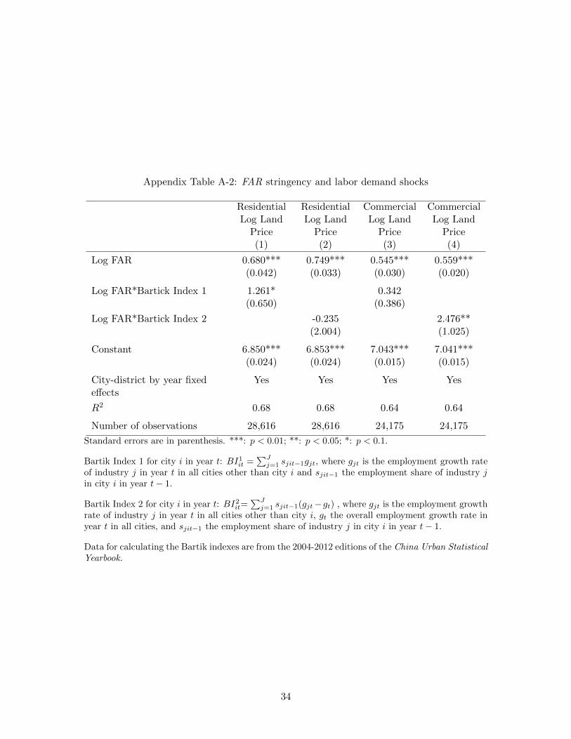
Appendix Table A-2: FAR stringency and labor demand shocks

ResidentialLog Land

Price(1)

ResidentialLog Land

Price(2)

CommercialLog Land

Price(3)

CommercialLog Land

Price(4)

Log FAR 0.680***(0.042)

0.749***(0.033)

0.545***(0.030)

0.559***(0.020)

Log FAR*Bartick Index 1 1.261*(0.650)

0.342(0.386)

Log FAR*Bartick Index 2 -0.235(2.004)

2.476**(1.025)

Constant 6.850***(0.024)

6.853***(0.024)

7.043***(0.015)

7.041***(0.015)

City-district by year fixedeffects

Yes Yes Yes Yes

R2 0.68 0.68 0.64 0.64

Number of observations 28,616 28,616 24,175 24,175

Standard errors are in parenthesis. ***: p < 0.01; **: p < 0.05; *: p < 0.1.

Bartik Index 1 for city i in year t: BI1it =∑J

j=1 sjit−1gjt, where gjt is the employment growth rateof industry j in year t in all cities other than city i and sjit−1 the employment share of industry jin city i in year t− 1.

Bartik Index 2 for city i in year t: BI2it=∑J

j=1 sjit−1(gjt−gt) , where gjt is the employment growthrate of industry j in year t in all cities other than city i, gt the overall employment growth rate inyear t in all cities, and sjit−1 the employment share of industry j in city i in year t− 1.

Data for calculating the Bartik indexes are from the 2004-2012 editions of the China Urban StatisticalYearbook.

34