Page 1

Measuring the conductivity of very dilute electrolyte solutions, drop by

drop

Leandro Martínez

Institute of Chemistry, University of Campinas, Campinas, Sao Paulo 13083-970, Brazil

ABSTRACT

The study of the conductivity of electrolyte solutions is important for practical applications and for the

understanding of ion mobility. Because of that, undergraduate experiments on ionic conductivity are

common practice in first year general chemistry or more advanced physical chemisdegreetry

laboratories. Often, the conductivities are measured for solutions prepared for various salts, in a range

of concentrations, and the relationship between solution conductivity and concentration is interpreted

in terms of the Kohlrausch law. Extrapolation of the molar conductivities to infinite dilution allows the

study of the individual ionic conductivities. In practice, the preparation of dilute solutions for these

experiments can be cumbersome, because small electrolyte contaminations can dominate the

conductivity of the solutions. Additionally, significant amounts of reactants, particularly deionized

water, must be used. Here, a simple experimental procedure is proposed to obtain the concentration

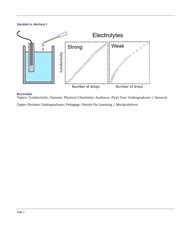
dependence of ionic conductivities for very dilute (sub-millimolar) electrolyte solutions. The experiment

consists in measuring the conductivity of solutions of increasing concentration prepared by dropping

the electrolyte solution into a single initial vessel of deionized water. The range of concentrations

achieved is one in which the conductivities vary linearly with the concentrations, such that the molar

conductivities can be obtained directly without the use of the Kohlrausch equation. The simplicity of

the experimental procedure leads the students to obtain very good quality results using minimal

amounts of materials. Examples are presented for the conductivities of various strong electrolytes, and

for weak acetic acid electrolyte, for which the conductivity is dependent on the degree of dissociation

even at very low concentrations.

Page 2

GRAPHICAL ABSTRACT

KEYWORDS

Topics: Conductivity; Domain: Physical Chemistry; Audience: First-Year Undergraduate / General;

Upper-Division Undergraduate; Pedagogy: Hands-On Learning / Manipulatives.

Page 3

The study of the conductivity of electrolyte solutions is important for the development of

electrochemical devices,1,2 for the characterization of the dissociation equilibrium of weak

electrolytes,2–4 and for the fundamental understanding of charge transport by ions.5 Therefore,

experiments in general chemistry and physical chemistry laboratories are widespread in

undergraduate chemistry courses, and are subject to many educational developments, from the

development of conductivity measuring apparatus to the preparation and study of specific

electrolytes.1,2

Typically, the conductivity 𝜅 of electrolyte solutions is measured for electrolyte solutions with

concentrations in the range of 10-3 to 10-1 mol L-1, as solutions in this range of concentrations can be

easily prepared.2,5,6 The molar conductivity Λ𝑚 (Λ𝑚 = 𝜅/𝑐) of strong electrolyte solutions can be nicely

fit by the Kohlrausch equation, 7

𝚲𝒎 = 𝚲𝒎∘ − 𝑲√𝒄

(1)

where Λ𝑚∘ is the molar conductivity at infinite dilution and c is the concentration of the solution. The

molar conductivity of weak electrolytes, on the other hand, is dependent on the degree of dissociation

of the electrolyte. At the limit of very dilute solutions, the Ostwald dilution law is expected to be

followed,

𝟏

𝚲𝐦=

𝟏

𝚲𝒎∘

+𝚲𝐦

(𝚲𝒎∘ )𝟐

𝑪𝑨

𝑲𝒅

(2)

The molar conductivity at infinite dilution can be decomposed into the contributions of each

ion,

𝚲𝒎∘ = 𝝂+𝝀+ + 𝝂−𝝀−

(3)

where 𝜆+ and 𝜆− are the ionic conductivities of the positive and negative ions, respectively, and 𝜈+ and

𝜈− are their stoichiometric coefficients in the salt molecular formula. From the concentration

dependence of the molar conductivity of each salt, it is possible to obtain the molar conductivities at

infinite dilution through Equation 1. If salts sharing the same ions are studied, it is possible to obtain

Page 4

by solving a linear system of equations the ionic conductivities, which are intrinsic properties of the

transport of each ion in the solvent studied.

Currently, portable conductivimeters with µS cm-1 sensitivity are accessible to undergraduate

laboratories, and are robust enough to be manipulated by students of any level. In principle, this

sensitivity would allow the study of electrolyte solutions with concentrations in the micromolar to

millimolar range. The difficulty in obtaining good quality conductivity measures is associated mainly to

the preparation of the solutions, manipulation, and cleaning of the apparatus, because small

contaminants of concentrated solutions of electrolytes can dominate the conductivity measures of

more dilute solutions. In the dynamics of an undergraduate laboratory experiment, with limited time

available, our experience is that many students fail to obtain conductivity measures which fit the

expected equations and the discussion of the results becomes impaired.

Here, a simple experimental procedure is proposed to perform a laboratory experiment on the

conductivity of electrolyte solutions at sub-millimolar concentrations. The procedure consists of

dropping the electrolyte solution to an initial volume of deionized water. The method saves significant

quantities of material and the results obtained are robust and reproducible.

Curriculum context

The strategy was practiced in laboratories of general chemistry and laboratories of physical chemistry

taught to students of Engineering and Chemistry of the University of Campinas (UNICAMP).

First-year undergraduate students of Mechanical Engineering were introduced to the concept

of ionic conductivity in the context of understanding electrolytic cells and ionic current. The

experiment was performed in the “QG100 – Chemistry” course of the University of Campinas, which

consists in a 2 hour lecture coupled to a 2 hour laboratory practice. In this case, the laboratory

practice was performed by a group of about 70 students which formed groups of 3 students. Each

group was responsible for conducting conductivity measures for a two different electrolytes. In this

Page 5

case, the outcome was that the students were able to probe and discuss qualitatively the differences in

ionic conductivities of different cations and anions, by comparing the results with the ones of other

groups.

The same experimental strategy was used in the “QF632 – Experimental Physical Chemistry I”

course of the Institute of Chemistry of the University of Campinas, which is taught to second year

undergraduates of the Chemistry course. Each practice consists of a two-hour lecture followed by a

four-hour practice. The experiment was performed by groups of 3 students, formed from classes of

about 30 students. In this case, given the greater student training and increased laboratory time, the

groups performed the conductivity measures for several (up to four) electrolytes, including a weak

electrolyte for every group. The students were then guided through the construction of Ostwald

dilution plots and the discussion on degrees of dissociation, conductivities, and ionic transport

mechanisms.

In both cases, the quality of the results obtained on the conductivity measures was similar to

that presented in this article. Since in the range of concentrations probed the conductivity of strong

electrolytes is linear with concentration, the possibility of decomposing the salt conductivity in

individual ionic conductivities can be discussed without appealing to ionic interactions and deviations

from ideality. Therefore, the students can readily associate the different salt conductivities with the

transport velocities of the ions in solution. These velocities can be discussed qualitatively or

quantitatively, depending on student background and lecture time.

EXPERIMENTAL PROCEDURE

In brief, the procedure consists on measuring the conductivity of solutions of electrolytes with

increasing concentration, which are prepared simply by dropping the stock electrolyte solution into a

sample of initially deionized water of known volume. The volume of the drop was determined

previously by weighing samples of 20 drops and averaging. The conductivity was measured after each

Page 6

drop addition, after a proper stabilization time. All the measurements were performed with solutions

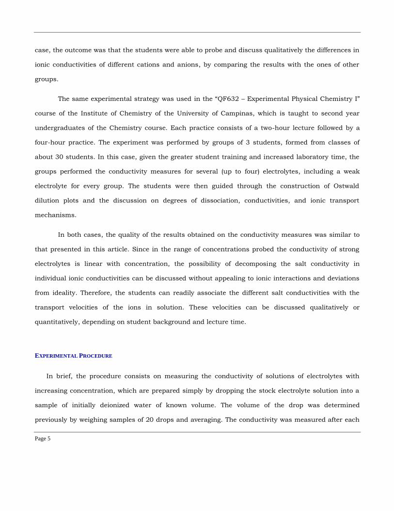
thermalized at the desired temperature (298K) by coupling to a thermal bath, as shown in Figure 1.

Additional experimental details, involving the careful cleaning and calibration of the conductivimeter

are similar to other procedures proposed for the study of electrolyte conductivities in general chemistry

and physical chemistry undergraduate laboratories, and are described in the Supplementary

Information.2,5

Figure 1. Experimental arrangement for conductivity measurements. The conductivimeter is placed inside a thermalized vessel containing deionized water.

Drops of an electrolyte solution are added to the system under constant stirring. The conductivity is measured after the addition of each drop, after a proper

delay for the homogenization of the solution and stabilization of the measured conductivity.

HAZARDS

The solutions used are usually very dilute and do not have significant hazard. Leftover solutions can

be disposed down the drain.

RESULTS AND DATA ANALYSIS

Page 7

Drop volume and error

The drop volume was estimated by measuring the mass of 20 drops and averaging for a single drop.

The densities of the solutions were considered to be the same of that of water at the same

temperature. Alternatively, they could be determined by the students. Five estimates of the drop

volume were obtained to compute an average, using each electrolyte solution studied.

A typical drop volume was of about 0.05 mL. The initial volume of water was proposed to be of

150 mL, such that the addition of 100 drops represented less than 4% of the total volume of the

solution. The students used a spreadsheet to compute the total volume of the solution after the

addition of each drop for computing the concentrations. At the same time, the error associated with

ignoring the volume of the solution added was discussed: If the electrolyte solution has a

concentration of 0.05 mol L-1, the concentration of the solution after the addition of the first drop is

~1.7 × 10-5 mol L-1. After the addition of 100 drops, the concentration rises to ~1.7 × 10-3 mol L-1. Thus,

most of the experiment was performed in the sub-millimolar concentration range.

As an advanced topic, the teacher might want to discuss how to estimate the variation in the

volume of a single drop from the standard deviation of the means measured. Indeed, each volume

estimate was obtained by averaging the volume of 20 drops. Therefore, the standard deviation

obtained between the estimates was the standard deviation of a mean. The standard deviation of

individual estimates (𝑆𝐷) is related to the standard deviation of the mean (𝑆𝐷�̄�) through 𝑆𝐷 = 𝑆𝐷�̄�√𝑁,

where N is the number of samples used to compute the mean.8 A typical result was to obtain a

standard deviation of the mean of the weights of 20 drops of 1-2%, such that the variation in the

volume of a single drop was of the order of 4-8%. The volume, and thus the concentration, error after

the addition of N drops was estimated as the standard error of the mean of N drops, and was of the

order of (4-8)/√𝑁%. The greatest error in the concentration estimate is associated to the addition of

the first drop, and was reasonably estimated to be below 10%, not compromising overall quality of the

results.

Page 8

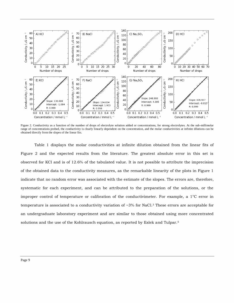
Strong electrolytes

The molar conductivity of strong electrolytes is expected to follow the Kohlrausch law (Equation 1). For

sufficiently dilute solutions, however, Λ𝑚∘ ≫ 𝐾√𝑐, and thus the molar conductivity is expected to be

approximately constant and equal to the molar conductivity at infinite dilution (Λ𝑚 ≈ Λ𝑚∘ ). In other

words, since 𝜅 = Λ𝑚𝑐, if one plots the conductivity 𝜅 as a function of the concentration, a linear

correlation with slope Λ𝑚∘ is expected.

In Figure 2 we display the results obtained by students at the regular course "QF632 -

Experimental Physical Chemistry – I" of the Institute of Chemistry of the University of Campinas

(UNICAMP), for strong electrolytes. The range of concentrations achieved was within 10-5 and 0.5×10-3

mol L-1 for the addition of up to 100 drops of 0.05 mol L-1 electrolyte solutions into initial deionized

water volumes varying between 150 and 250 mL, depending on the student's solution preparation

details. All experiments were performed at 298K, within the precision of the thermostatic bath

available. We plot here the conductivity as a function of the number of drops added or concentrations,

up to 0.5×10-3 mol L-1. In this range of concentrations, the linearity of the conductivity with the

concentration is clear, as shown in Figure 2, and suggests that the approximation that Λ𝑚∘ ≫ 𝐾√𝑐 can

be used. The data obtained can be fit by linear equations with correlation coefficients greater than

0.997 in all cases. The slopes provide directly the molar conductivity in this range of concentrations,

which is constant and expected to be a good approximation of the molar conductivity at infinite

dilution.

Page 9

Figure 2. Conductivity as a function of the number of drops of electrolyte solution added or concentrations, for strong electrolytes. At the sub-millimolar

range of concentrations probed, the conductivity is clearly linearly dependent on the concentration, and the molar conductivities at infinite dilutions can be

obtained directly from the slopes of the linear fits.

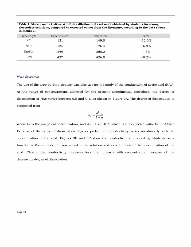
Table 1 displays the molar conductivities at infinite dilution obtained from the linear fits of

Figure 2 and the expected results from the literature. The greatest absolute error in this set is

observed for KCl and is of 12.6% of the tabulated value. It is not possible to attribute the imprecision

of the obtained data to the conductivity measures, as the remarkable linearity of the plots in Figure 1

indicate that no random error was associated with the estimate of the slopes. The errors are, therefore,

systematic for each experiment, and can be attributed to the preparation of the solutions, or the

improper control of temperature or calibration of the conductivimeter. For example, a 1°C error in

temperature is associated to a conductivity variation of ~3% for NaCl.3 These errors are acceptable for

an undergraduate laboratory experiment and are similar to those obtained using more concentrated

solutions and the use of the Kohlrausch equation, as reported by Eslek and Tulpar.5

Page 10

Table 1. Molar conductivities at infinite dilution in S cm2 mol-1 obtained by students for strong electrolyte solutions, compared to expected values from the literature, according to the data shown in Figure 1.

Electrolyte Experimental Expected Error

KCl 131 149.8 -12.6%

NaCl 135 126.4 +6.8%

Na2SO4 249 260.2 -4.3%

HCl 427 426.0 +0.2%

Weak electrolytes

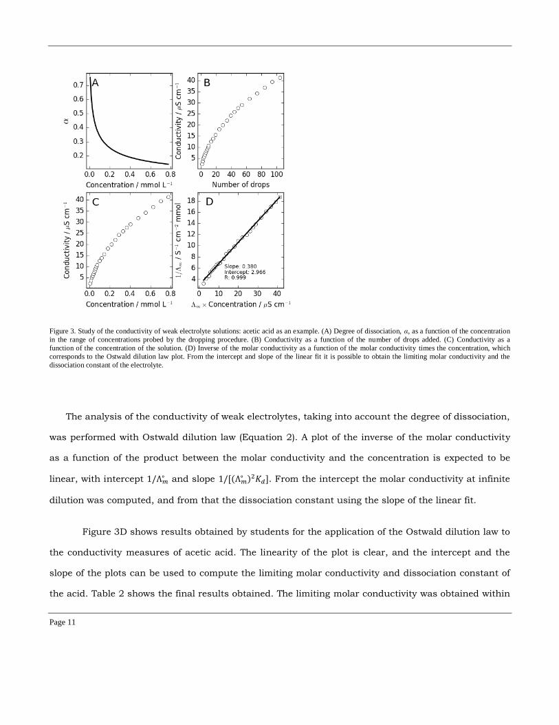
The use of the drop by drop strategy was also use for the study of the conductivity of acetic acid (HAc).

At the range of concentrations achieved by the present experimental procedure, the degree of

dissociation of HAc varies between 0.8 and 0.1, as shown in Figure 3A. The degree of dissociation is

computed from

𝐾𝑑 =𝛼2𝐶𝐴

1 − 𝛼

where 𝐶𝐴 is the analytical concentration, and Kd = 1.75×10-5, which is the expected value for T=298K.9

Because of the range of dissociation degrees probed, the conductivity varies non-linearly with the

concentration of the acid. Figures 3B and 3C show the conductivities obtained by students as a

function of the number of drops added to the solution and as a function of the concentration of the

acid. Clearly, the conductivity increases less than linearly with concentration, because of the

decreasing degree of dissociation.

Page 11

Figure 3. Study of the conductivity of weak electrolyte solutions: acetic acid as an example. (A) Degree of dissociation, α, as a function of the concentration

in the range of concentrations probed by the dropping procedure. (B) Conductivity as a function of the number of drops added. (C) Conductivity as a

function of the concentration of the solution. (D) Inverse of the molar conductivity as a function of the molar conductivity times the concentration, which

corresponds to the Ostwald dilution law plot. From the intercept and slope of the linear fit it is possible to obtain the limiting molar conductivity and the

dissociation constant of the electrolyte.

The analysis of the conductivity of weak electrolytes, taking into account the degree of dissociation,

was performed with Ostwald dilution law (Equation 2). A plot of the inverse of the molar conductivity

as a function of the product between the molar conductivity and the concentration is expected to be

linear, with intercept 1/Λ𝑚∘ and slope 1/[(Λ𝑚

∘ )2𝐾𝑑]. From the intercept the molar conductivity at infinite

dilution was computed, and from that the dissociation constant using the slope of the linear fit.

Figure 3D shows results obtained by students for the application of the Ostwald dilution law to

the conductivity measures of acetic acid. The linearity of the plot is clear, and the intercept and the

slope of the plots can be used to compute the limiting molar conductivity and dissociation constant of

the acid. Table 2 shows the final results obtained. The limiting molar conductivity was obtained within

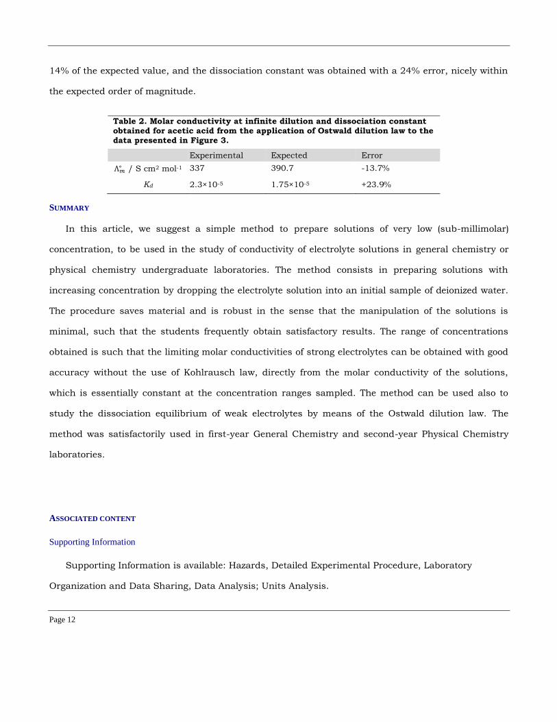
Page 12

14% of the expected value, and the dissociation constant was obtained with a 24% error, nicely within

the expected order of magnitude.

Table 2. Molar conductivity at infinite dilution and dissociation constant obtained for acetic acid from the application of Ostwald dilution law to the data presented in Figure 3.

Experimental Expected Error

Λ𝑚∘ / S cm2 mol-1 337 390.7 -13.7%

Kd 2.3×10-5 1.75×10-5 +23.9%

SUMMARY

In this article, we suggest a simple method to prepare solutions of very low (sub-millimolar)

concentration, to be used in the study of conductivity of electrolyte solutions in general chemistry or

physical chemistry undergraduate laboratories. The method consists in preparing solutions with

increasing concentration by dropping the electrolyte solution into an initial sample of deionized water.

The procedure saves material and is robust in the sense that the manipulation of the solutions is

minimal, such that the students frequently obtain satisfactory results. The range of concentrations

obtained is such that the limiting molar conductivities of strong electrolytes can be obtained with good

accuracy without the use of Kohlrausch law, directly from the molar conductivity of the solutions,

which is essentially constant at the concentration ranges sampled. The method can be used also to

study the dissociation equilibrium of weak electrolytes by means of the Ostwald dilution law. The

method was satisfactorily used in first-year General Chemistry and second-year Physical Chemistry

laboratories.

ASSOCIATED CONTENT

Supporting Information

Supporting Information is available: Hazards, Detailed Experimental Procedure, Laboratory

Organization and Data Sharing, Data Analysis; Units Analysis.

Page 13

AUTHOR INFORMATION

Corresponding Author

*E-mail: leandro@iqm.unicamp.br

ACKNOWLEDGMENTS

The author thanks the financial support of FAPESP (Grants 2010/16947-9, 2013/05475-7, and

2013/08293-7).

REFERENCES

(1) Set, S.; Kita, M. Development of a Handmade Conductivity Measurement Apparatus and Application to

Vegetables and Fruits. J. Chem. Educ. 2014, 91 (6), 892–897 DOI: 10.1021/ed400611q.

(2) Nyasulu, F.; Moehring, M.; Arthasery, P.; Barlag, R. K a and K b from pH and Conductivity Measurements: A

General Chemistry Laboratory Exercise. J. Chem. Educ. 2011, 88 (5), 640–642 DOI: 10.1021/ed100132m.

(3) Nyasulu, F.; Stevanov, K.; Barlag, R. Exploring Fundamental Concepts in Aqueous Solution Conductivity: A

General Chemistry Laboratory Exercise. J. Chem. Educ. 2010, 87 (12), 1364–1366 DOI: 10.1021/ed100385s.

(4) Eslek, Z.; Tulpar, A. Following Precipitation Reactions with Conductivity Measurements. J. Chem. Educ. 2013,

90 (12), 1668–1670 DOI: 10.1021/ed300594f.

(5) Eslek, Z.; Tulpar, A. Solution Preparation and Conductivity Measurements: An Experiment for Introductory

Chemistry. J. Chem. Educ. 2013, 90 (12), 1665–1667 DOI: 10.1021/ed300593t.

(6) Atkins, P.; de Paula, J. Physical Chemistry; W. H. Freeman, 2009.

(7) Garland, C. W.; Nibler, J. W.; Shoemaker, D. P. Experiment 17: Conductance of solutions. In: Experiments in

Physical Chemistry. 8th Ed. McGraw-Hill, 2009.

(8) Altman, D. G.; Bland, J. M. Standard deviations and standard errors. BMJ 2005, 331 (7521), 903 DOI:

10.1136/bmj.331.7521.903.

(9) Cohn, E. J.; Heyroth, F. F.; Menkin, M. F. THE DISSOCIATION CONSTANT OF ACETIC ACID AND THE

Page 14

ACTIVITY COEFFICIENTS OF THE IONS IN CERTAIN ACETATE SOLUTIONS 1. J. Am. Chem. Soc. 1928, 50

(3), 696–714 DOI: 10.1021/ja01390a012.