Measuring fractional charge and statistics in fractional quantum Hall fluidsthrough noise experiments

Eun-Ah Kim,1,2 Michael J. Lawler,1 Smitha Vishveshwara,1 and Eduardo Fradkin1

1Department of Physics, University of Illinois at Urbana-Champaign, 1110 West Green Street, Urbana, Illinois 61801-3080, USA2Stanford Institute for Theoretical Physics and Department of Physics, Stanford University, Stanford, California 94305, USA

�Received 13 April 2006; published 27 October 2006�

A central long standing prediction of the theory of fractional quantum Hall �FQH� states that it is a topo-logical fluid whose elementary excitations are vortices with fractional charge and fractional statistics. Yet, theunambiguous experimental detection of this fundamental property, that the vortices have fractional statistics,has remained an open challenge. Here we propose a three-terminal “T junction” as an experimental setup forthe direct and independent measurement of the fractional charge and statistics of fractional quantum Hallquasiparticles via cross current noise measurements. We present a nonequilibrium calculation of the quantumnoise in the T-junction setup for FQH Jain states. We show that the cross current correlation �noise� can bewritten in a simple form, a sum of two terms, which reflects the braiding properties of the quasiparticles: thestatistics dependence captured in a factor of cos � in one of two contributions. Through analyzing these twocontributions for different parameter ranges that are experimentally relevant, we demonstrate that the noise atfinite temperature reveals signatures of generalized exclusion principles, fractional exchange statistics andfractional charge. We also predict that the vortices of Laughlin states exhibit a “bunching” effect, while higherstates in the Jain sequences exhibit an “antibunching” effect.

DOI: 10.1103/PhysRevB.74.155324 PACS number�s�: 73.23.�b, 71.10.Pm, 73.50.Td, 73.43.Jn

I. INTRODUCTION

Bose-Einstein statistics of photons and Fermi-Dirac statis-tics of electrons hold keys to two major triumphs of quantummechanics: the explanation of the blackbody radiation �thatstarted quantum mechanics� and the periodic table. The spin-statistics theorem states that particles with integer �half-integer� spins are bosons �fermions� and that the correspond-ing second-quantized fields obey canonical equal timecommutation �anticommutation� relations. In three spatial di-mensions, the spin can only be integer or half-integer sincethe fields should transform as an irreducible representation ofthe Lorentz group SO�3, 1� �relativistic� or SO�3� �nonrela-tivistic�. Consequently particles in three-dimensional �3D�space have either bosonic or fermionic statstics. In one spa-tial dimension �1D� on the other hand, neither fermions norhardcore bosons can experience their statistics since theycannot go past each other. As a result, statistics is essentiallyarbitrary in one spatial dimension �which in some sense caneven be regarded as a matter of definition.� In particular, theexcitations of �integrable� one-dimensional systems are topo-logical solitons which have a two-body S matrix which ac-quires a phase factor upon the exchange of the positions ofthe solitons. In this sense, one can assign an intermediatestatistics to the solitons. However in two spatial dimensionsthe situation is quite different. It has long been known1,2 thatin two dimensions an intermediate form of statistics, frac-tional statistics is possible. A specific quantum mechanicalconstruction of a particle with fractional statistics, proposedand dubbed an anyon by Wilczek,2 consists of a particle ofcharge q bound to a solenoid with flux �, where q� bears anoninteger ratio to the fundamental flux quantum �0. In thispaper, we study the 2D setting of the quantum Hall system asan arena for displaying such fractional statistics, and proposea concrete experiment for measuring its effects.

Not long after the first observation of the fractional quan-tum Hall �FQH� effect,3 Laughlin proposed that the quasipar-

ticles �QP’s� and quasiholes �QH’s� of these incompressiblefluids carry a fractional charge e*= ±�e determined by theprecisely quantized Hall conductance �=1/ �2n+1� for aninteger n �for Laughlin states�4. Soon after, it was shown thatthese QP’s, would have fractional braiding statistics,5,6 i.e.,the two QP joint wave function would gain a complex valuedphase factor interpolating between 1 �boson� and −1�fermion� upon exchange:

��r1,r2� = ei���r2,r1� �1.1�

with 0����. In the anyonic picture, the statistical anglecorresponds to �=�q� /�0. Laughlin QP’s are a specific ex-ample with q=�. In order to compute the statistical angle �,Arovas et al.5 first considered the the adiabatic process ofone QP encircling another. By calculating the Berry phaseassociated with this process they showed that the two QPwave function ��r1 ,r2� gains an extra “statistical phase” ofei2�� in addition to the magnetic flux induced Aharonov-Bohm phase upon encircling. An adiabatic exchange of twoQP’s can be achieved by moving one QP only half its wayaround the other and shifting both of them rigidly to end upin interchanged initial positions. They thus argued that thephase factor picked up by a two QP joint wave function uponthis exchange process should be precisely half of what it isfor a round trip and hence �=��.

From a more general standpoint, anyons are excitationswhich carry a representation of the braid group �see below�.This is possible both for nonrelativistic particles in highmagnetic fields �as we will be interested in here� as well assome field-theoretic relativistic models. As in the FQH ex-ample, the quantum mechanical amplitudes for processes in-volving two or more of these particles �regarded as low-energy excitations from some more complicated system� arerepresented by world lines which never cross �as if they hada hard-core repulsion�. In �2+1� dimensions different histo-

PHYSICAL REVIEW B 74, 155324 �2006�

1098-0121/2006/74�15�/155324�23� ©2006 The American Physical Society155324-1

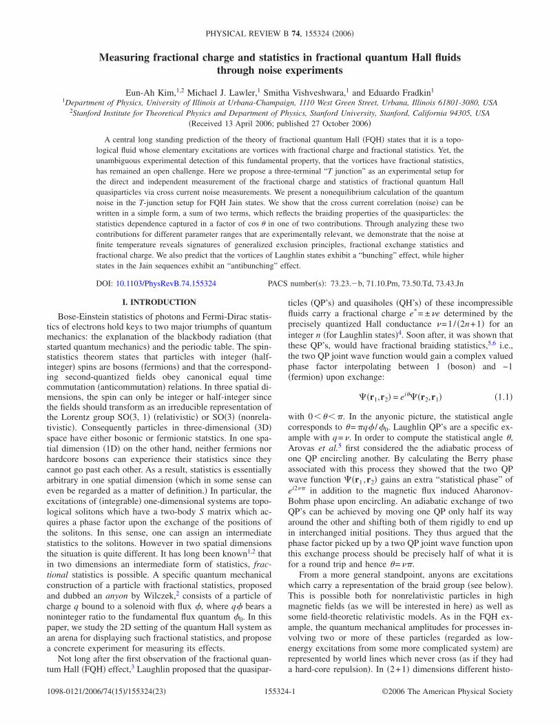
ries of these particles can be classified according to the to-pological invariants of the knots formed by their world lines�see Fig. 1�. These topological invariants are representationsof a group, the braid group. The statistical angle is one suchlabel and it corresponds to an Abelian �one-dimensional� rep-resentation of the braid group. Most quantum Hall states areAbelian �in this sense�. However a number of non-Abelianstates have been constructed �e.g., �=5/2, 12/5, and a fewothers�.

Fractional �or braid� statistics is a generalization of theconcept that fermions have wave functions which are oddupon exchange �i.e., thus they obey the Pauli exclusion prin-ciple� while bosons have wave functions which are odd uponexchange. The notion of statistics is �as its name indicates�also related to the problem of counting states. Some yearsago, Haldane7 introduced the concept of exclusion statistics,which is a generalization of the Pauli exclusion principle forfermions. Exclusion statistics in finite systems is determinedby how much an addition of a particle diminishes the numberof available states for yet another addition. For fermions, thenumber of states will diminish by 1 if a particle is added tothe system while for bosons, the number of states would staythe same; Haldane’s idea was to consider more general pos-sibilities interpolating between fermions and bosons. Al-though the Hilbert space counting definition of statistics andthe braiding definition of statistics coincide with one anotherfor Laughlin states, the two definitions are not equivalent ingeneral. It was argued by Haldane,7 and shown explicitly byVan Elburg and Schoutens,8 that the QP’s of the FQH statesalso obey a form of exclusion statistics.

Fractional charge and statistics are fundamental propertiesof QP’s emerging from the strongly interacting FQH liquid.Each of the filling factors � displaying precise quantizationof fractional Hall conductance �xy =�e2 /h represent a distinctphase characterized by nontrivial internal order—topologicalorder—which is robust against arbitrary perturbations.9,10

The measurement of fractional statistics will prove the exis-tence of such topological order. While there is substantialexperimental evidence for the fractional charge of these QP’sand QH’s,11–14 in particular from two-terminal noise experi-ments, similar evidence for statistical properties or the con-

nection between two distinct ways of determining statistics isstill lacking. The main challenge in detection of anyons is tomanipulate these “emergent particles” which cannot be takenoutside the 2D system and to measure the effect of statisticalphase. In this paper, we show that the noise in current fluc-tuations in a three-terminal geometry �a “T junction”� inFQH Jain states15 behaves as in a Hanbury-Brown and Twiss�HBT� interferometer16 with clear and independent signa-tures of fractional charge, fractional statistics and exclusionstatistics.

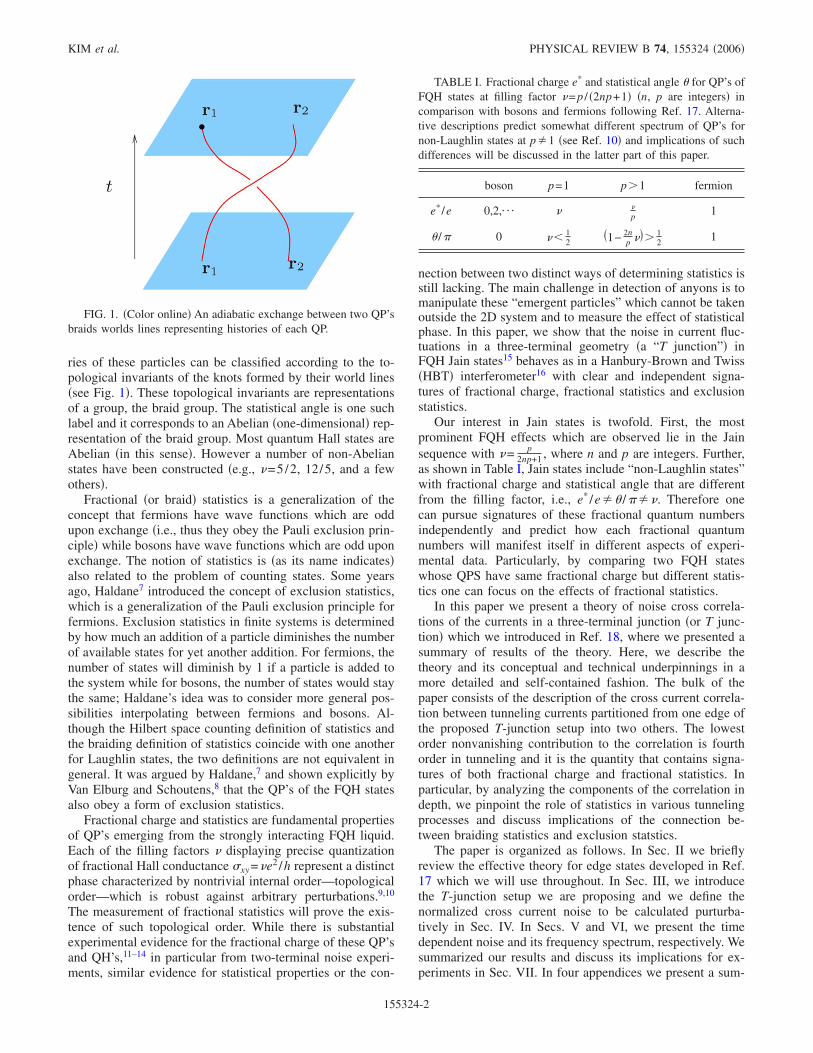
Our interest in Jain states is twofold. First, the mostprominent FQH effects which are observed lie in the Jainsequence with �= p

2np+1 , where n and p are integers. Further,as shown in Table I, Jain states include “non-Laughlin states”with fractional charge and statistical angle that are differentfrom the filling factor, i.e., e* /e�� /���. Therefore onecan pursue signatures of these fractional quantum numbersindependently and predict how each fractional quantumnumbers will manifest itself in different aspects of experi-mental data. Particularly, by comparing two FQH stateswhose QPS have same fractional charge but different statis-tics one can focus on the effects of fractional statistics.

In this paper we present a theory of noise cross correla-tions of the currents in a three-terminal junction �or T junc-tion� which we introduced in Ref. 18, where we presented asummary of results of the theory. Here, we describe thetheory and its conceptual and technical underpinnings in amore detailed and self-contained fashion. The bulk of thepaper consists of the description of the cross current correla-tion between tunneling currents partitioned from one edge ofthe proposed T-junction setup into two others. The lowestorder nonvanishing contribution to the correlation is fourthorder in tunneling and it is the quantity that contains signa-tures of both fractional charge and fractional statistics. Inparticular, by analyzing the components of the correlation indepth, we pinpoint the role of statistics in various tunnelingprocesses and discuss implications of the connection be-tween braiding statistics and exclusion statstics.

The paper is organized as follows. In Sec. II we brieflyreview the effective theory for edge states developed in Ref.17 which we will use throughout. In Sec. III, we introducethe T-junction setup we are proposing and we define thenormalized cross current noise to be calculated purturba-tively in Sec. IV. In Secs. V and VI, we present the timedependent noise and its frequency spectrum, respectively. Wesummarized our results and discuss its implications for ex-periments in Sec. VII. In four appendices we present a sum-

FIG. 1. �Color online� An adiabatic exchange between two QP’sbraids worlds lines representing histories of each QP.

TABLE I. Fractional charge e* and statistical angle � for QP’s ofFQH states at filling factor �= p / �2np+1� �n, p are integers� incomparison with bosons and fermions following Ref. 17. Alterna-tive descriptions predict somewhat different spectrum of QP’s fornon-Laughlin states at p�1 �see Ref. 10� and implications of suchdifferences will be discussed in the latter part of this paper.

boson p=1 p1 fermion

e* /e 0,2,¯ � �

p1

� /� 0 �� 12

�1− 2np �� 1

21

KIM et al. PHYSICAL REVIEW B 74, 155324 �2006�

155324-2

mary of the theory of the edge states that we use here �Ap-pendix A�, of the Schwinger-Keldysh technique andconventions �Appendix B�, some useful identities for vertexoperators �Appendix C�, and the unitary Klein factors �Ap-pendix D�.

II. AN EFFECTIVE THEORY FOR EDGE STATES

In this section, we summarize the properties of edge statesfor the Jain sequence and their associated quasiparticles.While the creation of QP excitations in the 2D bulk of FQHsystems has an associated energy gap �i.e., FQH liquid isincompressible�, the one-dimensional �1D� boundary definedby a confining potential can support gapless excitations.10,19

Further there is a striking one-to-one correspondence be-tween QP states in the bulk and at the edge making the FQHliquid holographic.19 Given that edge states comprise an ef-fective 1D system propagating only along the direction dic-tated by the magnetic field �a chiral Luttinger liquid10,19�,they can be described in terms of chiral bosons using thestandard bosonization approach. The edge effective Lagrang-ian density for Jain states, derived from the boundary term ofthe fermionic Chern-Simons theory20 by López andFradkin17 is given by

L0 =1

4���x�c�− �t�c − �x�c�

+ limvN→0+

1

4��x�N��t�N + vN�x�N� , �2.1�

where �c is a right moving charge mode whose speed is setto be vc=1 ��− with g=1/� and v=1 case of Appendix A�and �N is the nonpropagating charge neutral topologicalmode obtained as a vN→0+ limit of a right mover with gN=−1. Note that for the purpose of regularization and to care-fully keep track of short time behavior which is crucial forensuring the correct statistics, we shall keep a neutral modespeed vN and take the limit vN→0 only at the very end.

The normal ordered vertex operator creating a quasiparti-cle excitation on this edge, with fractional quantum numberstabulated in Table I, is given by17

† � :e−i��1/p��c+�1+�1/p��N�: � :e−i�: , �2.2�

where we define a short hand notation � to represent theappropriate linear combination of the charge mode and thetopological mode

�� �1

p�c +�1 +

1

p�N� . �2.3�

By noting the equal time commutator for the new field �being

���x,t�,��x�,t�� = i�� �p2 −

1

p− 1�sgn�x − x��

= − i� sgn�x − x�� �2.4�

the quantum numbers of † can be verified as follows. Thecharge density operator j0� 1

2��x�c measures the charge of

the QP operator since �j0�x� ,†�x���� e*

e �x−x��†�x��. Byexpanding the vertex operator Eq. �2.2�, this commutator canbe calculated order by order to give

�j0�x�,†�x��� =1

2���x�c�x�,e−i�1/p��c�x���

= −1

2�

i

p�x��c�x�,�c�x��� + ¯

=1

2�

��

p�x sgn�x − x�� + ¯

=�

p �x − x��†�x�� , �2.5�

hence e* /e= �p . As for statistics, using the Campbell-Baker-

Hausdorff �CBH� formula for exponential of operators A,

eAeB=eBeAe�A,B�, the statistical angle of the QP operator canbe calculated via exchange of QP positions at equal time asthe following:

†�x�†�x�� = †�x��†�x�e−���x�,��x���

= †�x��†�x�ei� sgn�x−x��, �2.6�

which confirms �= �1− 2np �� modulo 2�.

Combining charge mode and neutral mode propagator,one can obtain the propagator for the field �:

��x,t���0,0� =1

p2 �c�x,t��c�0,0� + �1 +1

p�

��N�x,t��N�0,0�

= −�

p2 ln� �0 + i�t − x��0

�+ i lim

vN→0+

�

2�1 +

1

p�sgn�vNt − x� .

�2.7�

From Eq. �2.7�, one arrives at the following form for the QPpropagator at zero temperature �see Appendix C�:

�x,t�†�0,0� = e��x,t���0,0�

= limvN→0+

� �0

�0 + i�t − x���/p2

e−i��/2��1+1/p�sgn�vNt−x�.

�2.8�

Equation �2.8� shows that the QP operators have the scalingdimension K

2 = �

2p2 = 12p�2np+1� . Further, as �→0+, the limit x

→0− of Eq. �2.8� becomes

�0−,t�†�0,0� = t

�0 −K

ei� sgn�t� �2.9�

with the explicit dependence on the statistical angle emerg-ing in the long wavelength limit. This equal position propa-gator, which explicitly encodes information on statistics,plays a prominent role in subsequent point-contact tunnelingcalculations. Most importantly, the amplitude of the propa-

MEASURING FRACTIONAL CHARGE AND STATISTICS… PHYSICAL REVIEW B 74, 155324 �2006�

155324-3

gator Eq. �2.9� is governed by the scaling dimension but thephase is solely determined by the statistical angle.

Since edge states are gapless excitations, they act as win-dows for experimental probes to observe features of the FQHdroplet. In particular, tunneling between edges allows a vi-able access to single QP properties, provided the tunnelingpath lie inside the FQH liquid �QP’s only exist within theliquid�.21 In fact, such tunneling has been successfully usedin a geometry hosting a single point contact and two edgesfor the detection of fractional charge through shot noisemeasurements.12–14 In principle, two edges would suffice foranyonic exchange as well with QP’s from each edge ex-changing positions via tunneling through the 2D FQH bulk.However, in order to detect the phase information, the pathof exchange needs to be intercepted, for instance, by insert-ing a third edge and allowing QP exchange between first twoedges to go through the third edge. This third edge thus actsat once as a stage and an “observation deck.” Further, if thefirst two edges are each adding/removing QP’s to the thirdedge, one should be able to see the generalized exclusionprinciple in action by probing the third edge. In the nextsection, we propose a “T-junction” interferometer as a mini-mal realization of such a situation.

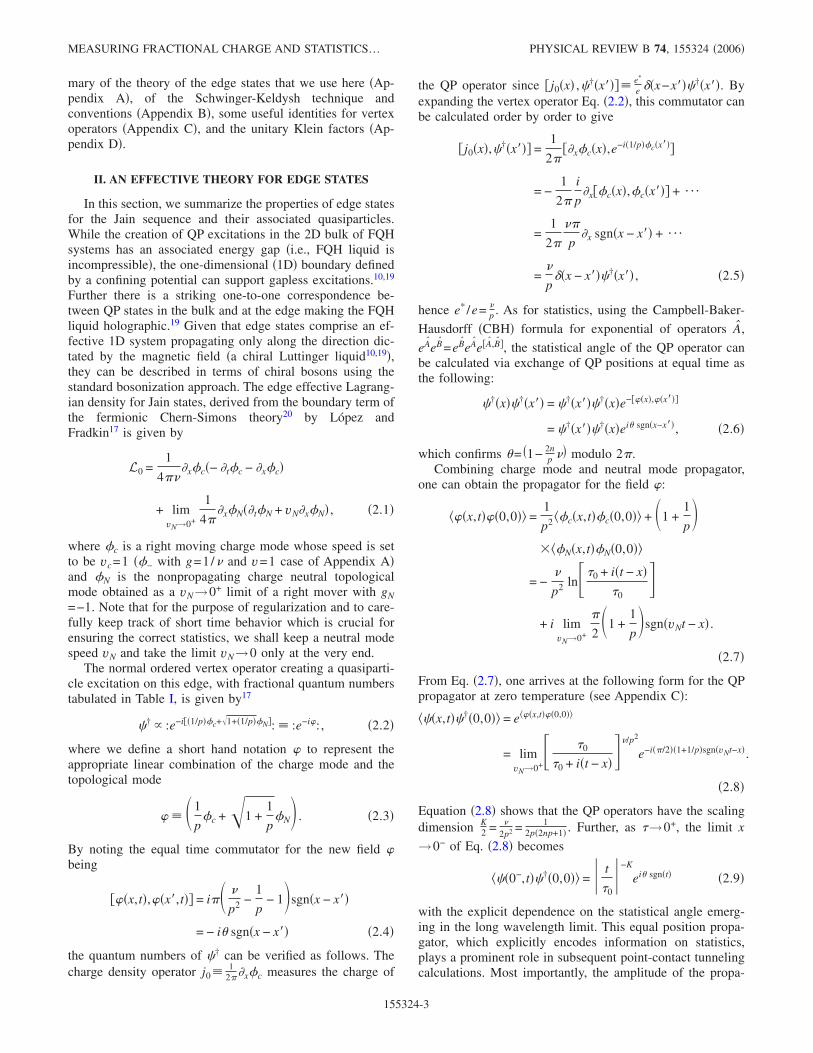
III. THE T-JUNCTION SETUP

In our proposed T-junction interferometer of the typeshown in Fig. 2, top gates can be used to define and bringtogether three edge states l=0,1 ,2 which are separated fromeach other by ohmic contacts. Two edges l=1 and l=2 eachseparately form tunnel junctions with edge 0 and upon set-ting the edge 0 at relative voltage V to the two others, QP’sare driven to tunnel between edge 0 and edges 1,2.

Denoting charge and neutral modes for edge l=0,1 ,2 by�c

l �xl , t� and �Nl �xl , t�, respectively, each edge state l in the

absence of tunneling �hence the superscript 0� can be de-scribed by Lagrangian densities of the form in Eq. �2.1�:

Ll�0� =

1

4���xl�c

l �− �t�cl − �xl

�cl � +

1

4���xl�N

l �t�Nl � ,

�3.1�

where xl now represents the curvilinear abscissa along eachedge, and the total Lagrangian density becomes

L�0� = �l=0,1,2

Ll�0�. �3.2�

Boson fields �cl and �N

l each have the same properties �suchas commutation relations and propagators� as �c and �N of asingle edge described in the Sec. II. Fields of different edgescommute with each other, i.e.,

��c/Nl ,�c/N

m � = 0, for l � m �3.3�

for l ,m=0,1 ,2. Within each edge l, a vertex operator ei�l,where �l again is a short hand notation � defined in Eq. �2.3�for each edge l, describes a QP excitation l

† in that edge.However, since �l’s are constructed to commute between dif-ferent edges, we need to introduce unitary Klein factors Flwith the appropriate algebra, as shown in the Appendix D, togive the correct QP statistics upon exchange between differ-ent edges. Hence, we have

l† =

1�2�a0

Flei��1/p��c

l +�1+�1/p��Nl � �

1�2�a0

Flei�l, �3.4�

where a0 is the short distance cutoff and the Klein factorsobey the statistical rules

FlFm = e−i�lmFmFl �3.5�

where �lm=−�ml and �02=�21=−�10=�. Notice the Kleinfactors do not affect the statistics between operators on thesame edge since �ll=0 from the requirement �lm=−�ml.

Now, if we set the the distance between two tunnelingpoints on edge 0 to be a small positive real number a �whichwe later send to zero� and the tunneling point on edge 1, 2 tobe the origin for the abscissa coordinate of edge 1, 2, thenQP’s tunnel at two locations x0=−a /2�X1 and x0=a /2�X2 on edge 0 and at x1=0, x2=0 on edges 1, 2. The opera-

tor Vj�t� which tunnels one QP from the edge 0 to edges j=1,2 at time t can then be written in the following form:

Vj†�t� � 0�Xj,t� j

†�0,t� = F0Fj−1ei�0�Xj,t�e−i�j�0,t�. �3.6�

The additional term in the Lagrangian due to the presence ofthe tunneling can be written as Lint=Lint,1+Lint,2 �Refs. 22and 23� with tunneling term involving edges j=1,2 given by

Lint,j�t� = − � jVj†�t� + H.c., �3.7�

where � j is the tunneling amplitude between edges 0 and j=1,2. The nonequilibrium situation of setting a constant dcvoltage bias V between edges 0 and j corresponds to substi-tuting � j by � je

−i�0t in Eq. �3.7�, where the Josephson fre-quency is explicitly determined by the fractional charge to be�0�e*V /� �the Peierls substitution22,24,25�. Using theHeisenberg equations of motion for the total charge Ql

=�dxlj0l�xl� of edge l where j0l�xl�= 12��x�c

l is the chargedensity operator for edge l, as was done by Chamon24,25 for

FIG. 2. �Color online� The proposed T-junction setup. Solid�blue� lines represent edge states where the edge state 0 is held atpotential V relative to edges 1 and 2, i.e., V0−V1=V0−V2=V.Dashed �red� lines show paths of two quasiparticle tunnelingthrough a FQH liquid from edge state 0 to edge 1 at x0=−a /2�X1, x1=0; from edge 0 to edge 2 at x0=a /2�X2, x2=0. Thedirect tunneling between edge 1 and 2 is turned off by setting thetwo edges at equal potential.

KIM et al. PHYSICAL REVIEW B 74, 155324 �2006�

155324-4

Laughlin states, one can show that the tunneling current op-

erator I j�t� from edge 0 to edge j is given by

I j�t� = ie*

�� j�ei�0tVj

† − e−i�0tVj� ,

�ie*��=±�� je

i��0tVj���, �3.8�

where we assumed � j to be real and introduced the notation

Vj†� Vj

�+� and Vj � Vj�−�, i.e.,

Vj����t� = �F0Fj

−1��ei��0�Xj,t�e−i��j�0,t�, �3.9�

to represent the summation over hermitian conjugates in acompact form. Notice that �=+ corresponds to a QP tunnel-ing from the edge j to 0 and �=− corresponds to a reversedirection tunneling.

We treat the nonequilibrium situation within theSchwinger-Keldysh formalism22–28 for computing expecta-tion values of operators. As a simple example, the expecta-tion value of the current on edge j takes the following formup to a normalization factor:

Ij =1

2 ��=±

TKIj�t��ei�KLint,j�tj�dtj0, �3.10�

where � labels the branch of the Keldysh contour: �=+ forthe forward branch �t=−�→�� and �=− for the backwardbranch �t=�→−��. TK indicates that the operators insidebrackets should be contour ordered before taking the expec-tation value, and 0 indicates the expectation value with re-spect to the free action S0=�Kdt�d3xL0 where the free La-grangian density L0 was given in Eq. �3.2�.

Our goal is to identify a measurable quantity that dis-tinctly captures the role of the statistical angle � which fea-tures in the single QP operator shown in Eq. �2.6�. The nor-malized cross correlation �noise� S�t� between tunnelingcurrent fluctuations ��Il= Il− Il�:

S�t − t�� ��I1�t��I2�t��

I1I2�3.11�

turns out to be the simplest quantity that can exhibit thesubtle signatures of statistics and distinguish them fromthose of fractional charge. In fact, in contrast to shot noise,this cross current correlation S�t− t�� carries statistical infor-mation even at the lowest nontrivial order, which we calcu-late perturbatively in the next section.

IV. PERTURBATIVE CALCULATION

In this section, we perform a detailed analysis of the nor-malized cross correlation at fourth �lowest nonvanishing�order in tunneling. We calculate the two point correlation andfour point correlation functions required to calculate thecross correlation in terms of edge state properties. We ana-lyze the detailed behavior of the cross correlation over dif-ferent Keldysh time domains and pinpoint the effects of sta-tistics, specifically drawing the connection between braiding

statistics and exclusion statistics. We show that cross corre-lation can be expressed in terms of two universal scalingfunctions and that the statistical dependence ultimately takeson a remarkably simple form.

It must be remarked that since the perturbation introducedin Eq. �3.7� is relevant in the renormalization group sense,perturbation theory is valid only under certain conditions.Specifically, perturbation holds as long as energies involved,such as voltage and temperature, are higher than a crossoverenergy scale proportional to �1/�1−K�. For energies muchlower than this cross-over scale, QP tunneling between edgesbecomes large enough to break the Hall droplet into smallerdisconnected regions and one needs an appropriate dual pic-ture to properly address the strong coupling fixed point. Forobserving the effects of statistics as prescribed by the corre-lation calculated here, it is imperative that the system re-mains in the perturbative regime.

The unnormalized cross correlation I1I2S�t− t��= �I1�t��I2�t��, where ¯ represents expectation valuewith respect to the full Lagrangian in the presence of tunnel-ing events, can be written in terms of expectation values withrespect to the free theory 0¯ as

I1I2S�t − t��

=1

4 ��,��

TKI1�t��I2�t����ei�KLint,1�t1�dt1+i�KLint,2�t2�dt20

−1

4 ��,��

TKI1�t��ei�KLint,1�t1�dt10

�TKI2�t����ei�KLint,2�t2�dt20. �4.1�

By expanding the exponentials in Eq. �4.1�, we can cal-culate the cross correlation perturbatively in the tunnelingamplitude � j. Since the tunneling operator is relevant in theRG sense �its scaling dimension is less than 1�, the perturba-tion theory will break down in the infrared �IR� limit. How-ever, the finite temperature in our case provides a natural IRcutoff making this perturvative calculation meaningful. Infact, we will show in the following sections that the strongeststatistical dependence is obtained at temperatures compa-rable to the bias voltage.

Clearly the lowest nonvanishing term in the perturbationexpansion is of order ��1�2�2. Using the expression for thetunneling current operator in Eq. �3.8�, the first term of Eq.�4.1� to this order can be written as

I1�t�I2�t���2� � �− i�2�ie*�21

4 ��,��,�1,�2

��,��

����1�2��1�2�2

�� dt1dt2ei��0�t−t1�+i���0�t�−t2�

� TKV1����t��V2

�����t����V1�−���t1

�1�V2�−����t2

�2�0,

�4.2�

where we used the fact that the Keldysh contour time-integral in the exponent can be represented using the contourbranch index ��

MEASURING FRACTIONAL CHARGE AND STATISTICS… PHYSICAL REVIEW B 74, 155324 �2006�

155324-5

�K

dt = ���=±

��� dt �4.3�

and the charge neutrality condition discussed in Appendix Cwhich enforces �1=−� and �2=−��. Similarly, the expecta-tion value of the current for the second term of Eq. �4.1�becomes

I1�2� =1

2 ��=±1

��,�1

�− i��ie*���1

�� dt1���1�2ei��0�t−t1�TKV1����t��V1

�−���t1�1�0� .

�4.4�

Putting Eqs. �4.2� and �4.4� together, we arrive at the follow-ing expression for the lowest nonvanishing term of the un-normalized cross current correlation

I1I2S�2��t − t�� =1

4�e*�2 �

�,��,�1,�2

��,��

����1�2��1�2�2

�� dt1dt2ei��0�t−t1�+i���0�t�−t2�

� �TKV1����t��V2

�����t����V1�−���t1

�1�

�V2�−����t2

�2�0 − TKV1����t��V1

�−���t1�1�0

�TKV2�����t����V2

�−����t2�2�0� . �4.5�

We now evaluate the two point function and the four pointfunction, and then combine them to obtain a simplified for-mula for I1I2S�2��t− t�� from Eq. �4.5�.

A. The two point function

Using Eq. �3.6� and the result of Appendix C to calculatethe chiral boson vertex correlation function, we find

TKV1����t��V1

�−���t1�1�0 = �F0F1

−1���F0F1−1�−�

�TKei��0�X1,t��e−i��0�X1,t1�1�

� TKei��1�0,t��e−i��1�0,t1�1� �4.6�

=exp�G�,�1�0,t − t1��

�exp�G�,�1�0,t − t1�� , �4.7�

where G�,���x−x� , t− t���TK�l�x , t���l�x� , t����0 is theKeldysh ordered and regulated �l propagator for all l whichwill be discussed below in detail for both zero temperatureand finite temperatures. Here we also used the fact that �l’sare independent from each other for different l’s. Notice thatthe Klein factor contribution simply becomes an identity for

a two point function of the tunneling operator V1. Hence,Klein factors are not necessary in calculations involving twopoint functions alone, and in fact, this is the reason that thelowest order contribution to shot noise does not contain sta-tistical information. However, as we show below, Klein fac-tors have nontrivial contributions in the four point functionwhich appears in the first term of Eq. �4.1�.

We now focus on the form of G�,���−a , t− t�� in the limita→0+. From the detailed analysis of Appendix B, the con-tour ordered propagators for �c and �N takes the followingforms at finite temperatures:

TK�c�x,t���c�x�,t���� = − � ln� sin�

���0 + i��,���t − t����t − t�� − �x − x����

��0

�� �4.8�

TK�N�x,t���N�x�,t���� = limvN→0+

− i�

2��,�� sgn�vN�t − t�� − �x − x��� . �4.9�

Hence the contour ordered propagator for � represented by G in Eqs. �4.7� and �4.18� can be written as

G�,���− a,t − t�� = −�

p2 ln� sin�

���0 + i��,���t − t���t − t� + a��

��0

�� + lim

vN→0+i�

2�1

p+ 1���,���t − t��sgn�vN�t − t�� + a� .

�4.10�

For the case of interest, i.e., a→0+ in the limit �0→0+, the above takes the following form �see Appendix B�:

KIM et al. PHYSICAL REVIEW B 74, 155324 �2006�

155324-6

G�,���0−,t − t�� = ln C�t − t�;T,K� + i

�

2��,���t − t��sgn�t − t�� ,

�4.11�

where we have introduced a notation for the amplitude of theQP propagator that depends on the temperature T and thescaling dimension K=� / p2:

C�t;T,K� ����0�K

�sinh �kBTt�K�4.12�

and defined

��,���t − t�� � �� + ��

2sgn�t − t�� −

� − ��

2� . �4.13�

We can now calculate the expectation value of the tunnel-ing current I1 of Eq. �4.4� to order O��1

2� using Eqs. �4.7�and �4.10�,

I1�t���2� = e*��1�2��

�� dt1ei��0�t−t1�����C�t − t1�2

�4.14�

with the statistical factor

���� = ���1

�1ei���,�1�t−t1�sgn�t−t1�� = 2i sin � . �4.15�

Notice that the resulting I1�t�� is independent of � and is aconstant independent of t, as applicable for a steady statecurrent.

B. The four point function

Following a procedure similar to the one that led up to Eq.�4.7�, we find that the four point function becomes

TKV1����t��V2

�����t����V1�−���t1

�1�V2�−����t2

�2�0

= TKei��0�X1,t��ei���0�X2,t����e−i��0�X1,t1�1�e−i���0�X2,t2

�2�0TKei��1�0,t��e−i��1�0,t1�1�0

�TKei���2�0,t����e−i���2�0,t2�2�0TK�F0F1

−1���F0F2−1����F0F1

−1�−��F0F2−1�−��0 �4.16�

=e�G�,�1�0,t−t1�+G��,�2

�0,t�−t2�+���G�,�2�−a,t−t2�+���G���1

�−a,t�−t1�−���G����a,t−t��−���G�1�2�−a,t1−t2��

�eG��1�0,t−t1�eG���2

�0,t�−t2�TK�F0F1−1���F0F2

−1����F0F1−1�−��F0F2

−1�−��0 �4.17�

=e2�G��1�0,t−t1�+G���2

�0,t�−t2�� e����G�,�2�−a,t−t2�+G���1

�a,t�−t1��

e����G����−a,t−t��+G�1�2�−a,t1−t2��

TK�F0F1−1���F0F2

−1����F0F1−1�−��F0F2

−1�−��0,

�4.18�

where we used Eq. �C6� for the case N=4 to calculate thefour vertex correlator for the second equality and used thefact that X1−X2=−a.

The factor involving four sets of Klein factors of the form�F0Fj

−1�± in the Eq. �4.18� has to be appropriately rearrangedthrough proper exchange rules �D2� and �D5� as the tunnel-

ing operators Vj�t��’s get rearranged for Keldysh contour or-dering. Since contour ordering depends on time arguments ofthe tunneling operators, Klein factors effectively become en-dowed with dynamics in the sense that where each of thesefour times fall on the contour determines whether Klein fac-tors associated with tunneling at each time have to be movedor not.23 In order to rearrange four sets of combined Kleinfactors of the form �F0Fj

−1���t�� involved in Eq. �4.18�, wehave to take six different possible pairs and contour orderwithin each pair. This process can be thought of as a full“contraction” where pairs of Klein factors can be treated akinto propagators.

These contour ordered Klein factor “propagators” werecalculated in Appendix D to be

TK�F0F1−1���t���F0F2

−1����t����0 = ei�����/2�sgn�X1−X2���,���t−t��

= e−i�����/2���,���t−t�� �4.19�

TK�F0F2−1���t���F0F1

−1����t����0 = ei�����/2� sgn�X2−X1���,���t−t��

= e−i�����/2����,��t�−t�, �4.20�

where ��,���t� is defined in Eq. �4.13�. Further using the factthat F0Fj

−1 commutes with itself gives

TK�F0Fj−1���t���F0Fj

−1�−���t����0 = 1. �4.21�

Expressing the Klein factor contribution in Eq. �4.18� interms of the six possible pairs and using their forms given byEqs. �4.20� and �4.21� simplifies it to the form

MEASURING FRACTIONAL CHARGE AND STATISTICS… PHYSICAL REVIEW B 74, 155324 �2006�

155324-7

e−i�����/2���,�2�t−t2�e−i�����/2���1,���t1−t��

e−i�����/2���,���t−t��e−i�����/2���1,�2�t1−t2�

. �4.22�

Hence, we can rewrite the four point function of Eq. �4.18� as

TKV1����t��V2

�����t����V1�−���t1

�1�V2�−����t2

�2�0 = e2�G��1�0,t−t1�+G���2

�0,t�−t2��e����G�,�2

�−a,t−t2�−i��/2���,�2�t−t2�+G�1,���−a,t1−t��−i��/2���1,���t1−t���

e����G�,���−a,t−t��−i��/2���,���t−t��+G�1,�2�−a,t1−t2�−i��/2���1,�2

�t1−t2��,

�4.23�

where we used the fact that G�,���x−x� , t− t��=G��,��x�−x , t�− t�, as is pointed out in Appendix B, to replaceG��,�1

�a , t�− t1� by G�1,���−a , t1− t��.Furthermore, observing the following:

G�,���0−,t − t�� − i

�

2��,���t − t��

= − K ln� sinh���t − t���

���0

�� + i

�

2��1 − sgn�t − t���

�4.24�

=G�,−��0−,t − t�� , �4.25�

where we have used Eqs. �4.11� and �4.13�, the four pointfunction of Eq. �4.23� further simplifies to the final form

TKV1����t��V2

�����t����V1�−���t1

�1�V2�−����t2

�2�0

= e2�G��1�0,t−t1�+G���2

�0,t�−t2��

�e����G�,−��0−,t−t2�+G�1,−�1

�0−,t1−t���

e����G�,−��0−,t−t��+G�1,−�1�0−,t1−t2��

�4.26�

����0�2K

sinh��t − t1��

2K

���0�2K

sinh��t� − t2��

2K

�

sinh��t1 − t2��

�K sinh��t − t���

�K sinh

��t1 − t���

�K sinh��t − t2��

�K�ei�

��,��,�1,�2�t,t�,t1,t2�, �4.27�

where we defined ����� noting that Eq. �4.23� depends onlyon the product ��� and collected all contributions to thephase factor by defining the following function:

���,��,�1,�2�t,t�,t1,t2�

� ���,�1�t − t1� + ����,�2

�t� − t2�

− ��

2�� sgn�t − t2� − � sgn�t − t���

− ��

2��1 sgn�t1 − t�� − �1�t1 − t2�� �4.28�

=− ��

2�sgn�t − t1� + � sgn�t − t2�

− � sgn�t − t�� − 1� + ���

2

��1 − sgn�t� − t2�� − �1�

2

��− sgn�t − t1� + � sgn�t1 − t��

− � sgn�t1 − t2� − 1� + �2�

2

��1 + sgn�t� − t2�� . �4.29�

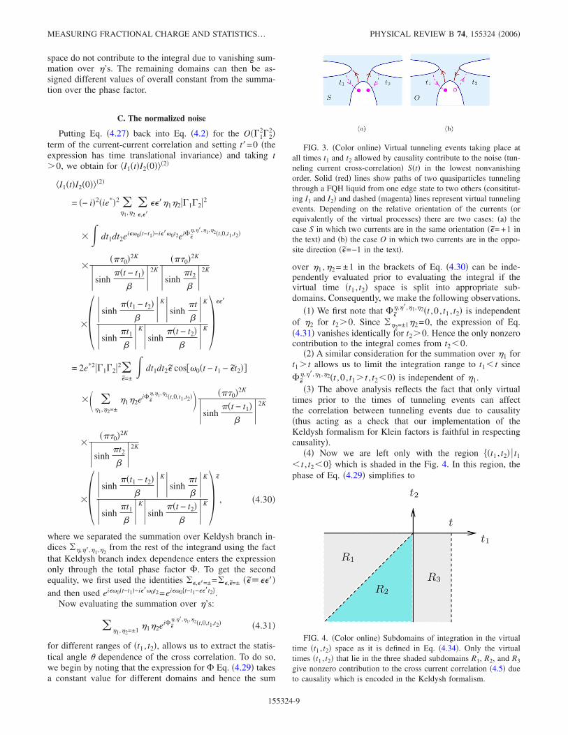
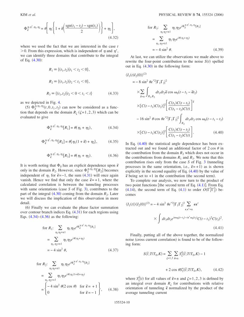
Note that ����� depends only on the relative directionsof tunneling, that is �= +1 for correlations between contribu-tions to I1 and I2 in the same orientation ��=��� and �=−1for correlations between contributions to I1 and I2 in theopposite orientation ��=−���. Each case of �=± is illustratedin Fig. 3 labeled S /O, respectively. The fact that the phasefactor � depends on these relative orientations allows us tounderstand the statistical angle dependent contribution to thenoise in connection with exclusion statistics7 as we will dis-cuss in the next section. Another important observation to bemade in Eq. �4.29� is that the time dependence of the phasefactor is such that it only depends on the sign of various timedifferences. Hence as we integrate over virtual times t1 andt2, to evaluate I1�t�I2�0� according to Eq. �4.2�, the domainof integration in �t1 , t2� space can be divided into subdomainsas shown in Fig. 4 and the phase factors for a given set ofKeldysh branch indices �’s and relative orientation of tun-neling � may be computed. Since integration is additive, wecan consider each domain’s contribution separately and lateradd them up to unravel the effect of the phase factor. Asimple analysis to follow shows that large parts of the �t1 , t2�

KIM et al. PHYSICAL REVIEW B 74, 155324 �2006�

155324-8

space do not contribute to the integral due to vanishing sum-mation over �’s. The remaining domains can then be as-signed different values of overall constant from the summa-tion over the phase factor.

C. The normalized noise

Putting Eq. �4.27� back into Eq. �4.2� for the O��12�2

2�term of the current-current correlation and setting t�=0 �theexpression has time translational invariance� and taking t0, we obtain for I1�t�I2�0��2�

I1�t�I2�0��2�

= �− i�2�ie*�2 ��1,�2

��,��

����1�2��1�2�2

�� dt1dt2ei��0�t−t1�−i���0t2ei���,��,�1,�2�t,0,t1,t2�

����0�2K

sinh��t − t1��

2K

���0�2K

sinh�t2

� 2K

�� sinh��t1 − t2��

K sinh�t

� K

sinh�t1

� K sinh

��t − t2��

K����

= 2e*2��1�2�2��=±

� dt1dt2� cos��0�t − t1 − �t2��

�� ��1,�2=±

�1�2ei���,�1,�2�t,0,t1,t2�� ���0�2K

sinh��t − t1��

2K

����0�2K

sinh�t2

� 2K

�� sinh��t1 − t2��

K sinh�t

� K

sinh�t1

� K sinh

��t − t2��

K��

, �4.30�

where we separated the summation over Keldysh branch in-dices ��,��,�1,�2

from the rest of the integrand using the factthat Keldysh branch index dependence enters the expressiononly through the total phase factor �. To get the secondequality, we first used the identities ��,��=±=��,�=± �������and then used ei��0�t−t1�−i���0t2 =ei��0�t−t1−���t2�.

Now evaluating the summation over �’s:

��1,�2=±1�1�2ei�

��,��,�1,�2�t,0,t1,t2� �4.31�

for different ranges of �t1 , t2�, allows us to extract the statis-tical angle � dependence of the cross correlation. To do so,we begin by noting that the expression for � Eq. �4.29� takesa constant value for different domains and hence the sum

over �1 ,�2= ±1 in the brackets of Eq. �4.30� can be inde-pendently evaluated prior to evaluating the integral if thevirtual time �t1 , t2� space is split into appropriate sub-domains. Consequently, we make the following observations.

�1� We first note that ���,��,�1,�2�t ,0 , t1 , t2� is independent

of �2 for t20. Since ��2=±1�2=0, the expression of Eq.�4.31� vanishes identically for t20. Hence the only nonzerocontribution to the integral comes from t2�0.

�2� A similar consideration for the summation over �1 fort1 t allows us to limit the integration range to t1� t since

���,��,�1,�2�t ,0 , t1 t , t2�0� is independent of �1.�3� The above analysis reflects the fact that only virtual

times prior to the times of tunneling events can affectthe correlation between tunneling events due to causality�thus acting as a check that our implementation of theKeldysh formalism for Klein factors is faithful in respectingcausality�.

�4� Now we are left only with the region ��t1 , t2� � t1

� t , t2�0� which is shaded in the Fig. 4. In this region, thephase of Eq. �4.29� simplifies to

FIG. 3. �Color online� Virtual tunneling events taking place atall times t1 and t2 allowed by causality contribute to the noise �tun-neling current cross-correlation� S�t� in the lowest nonvanishingorder. Solid �red� lines show paths of two quasiparticles tunnelingthrough a FQH liquid from one edge state to two others �consititut-ing I1 and I2� and dashed �magenta� lines represent virtual tunnelingevents. Depending on the relative orientation of the currents �orequivalently of the virtual processes� there are two cases: �a� thecase S in which two currents are in the same orientation ��= +1 inthe text� and �b� the case O in which two currents are in the oppo-site direction ��=−1 in the text�.

FIG. 4. �Color online� Subdomains of integration in the virtualtime �t1 , t2� space as it is defined in Eq. �4.34�. Only the virtualtimes �t1 , t2� that lie in the three shaded subdomains R1, R2, and R3

give nonzero contribution to the cross current correlation �4.5� dueto causality which is encoded in the Keldysh formalism.

MEASURING FRACTIONAL CHARGE AND STATISTICS… PHYSICAL REVIEW B 74, 155324 �2006�

155324-9

���,��,�1,�2 = ���1�1 + �� sgn�t1 − t2� − sgn�t1�

2�� + �2� ,

�4.32�

where we used the fact that we are interested in the case t0. From this expression, which is independent of � and ��,we can identify three domains that contribute to the integralof Eq. �4.30�:

R1 � ��t1,t2��t1� t2� 0� ,

R2 � ��t1,t2��t2� t1� 0� ,

R3 � ��t1,t2��t2� 0� t1� t� �4.33�

as we depicted in Fig. 4.�5� ��

�,�1,�2�t ,0 , t1 , t2� can now be considered as a func-tion that depends on the domain R� ��=1,2 ,3� which can beevaluated to give

���,��,�1,�2�R1� = ���1 + �2� , �4.34�

���,��,�1,�2�R2� = ���1�1 + �� + �2� , �4.35�

���,��,�1,�2�R3� = ���1 + �2� . �4.36�

It is worth noting that �� has an explicit dependence upon �only in the domain R2. However, since ��

�,�1,�2�R2� becomesindependent of �1 for �=−1, the sum �4.31� will once againvanish. Hence we find that only the case �= +1, where thecalculated correlation is between the tunneling processeswith same orientations �case S of Fig. 3�, contributes to thepart of the integral �4.30� coming from the domain R2. Laterwe will discuss the implication of this observation in moredetail.

�6� Finally we can evaluate the phase factor summationover contour branch indices Eq. �4.31� for each regions usingEqs. �4.34�–�4.36� as the following:

for R1: ��1�2=±1

�1�2ei���,��,�1,�2�R1�

= ��1,�2=±1

�1�2ei���1+�2�

= − 4 sin2 � , �4.37�

for R2: ��1�2=±1

�1�2ei���,��,�1,�2�R2�

= ��1,�2=±1

�1�2ei���1�1+��+�2�

= �− 4 sin2 ��2 cos �� for � = + 1

0 for � = − 1� , �4.38�

for R3: ��1�2=±1

�1�2ei���,��,�1,�2�R3�

= ��1,�2=±1

�1�2ei���1+�2�

= − 4 sin2 � . �4.39�

At last, we can utilize the observations we made above torewrite the four-point contribution to the noise S�t� spelledout in Eq. �4.30� in the following form:

I1�t�I2�0��2�

= − 8 sin2 �e*2��1�2�2

���=±�

R1,R3

dt1dt2� cos �0�t − t1 − �t2�

��C�t − t1�C�t2��2�C�t1�C�t − t2�C�t1 − t2�C�t�� �

− 16 sin2 � cos �e*2��1�2�2�R2

dt1dt2 cos �0�t − t1 − t2�

��C�t − t1�C�t2��2�C�t1�C�t − t2�C�t1 − t2�C�t�� . �4.40�

In Eq. �4.40� the statistical angle dependence has been ex-tracted out and we found an additional factor of 2 cos � inthe contribution from the domain R2 which does not occur inthe contributions from domains R1 and R3. We note that thiscontribution rises only from the case S of Fig. 3 �tunnelingprocesses in the same orientation, i.e., �= +1� as is shownexplicitly in the second equality of Eq. �4.40� by the value of� being set to +1 in the contribution �the second term�.

To complete our analysis, we now turn to the product oftwo point functions �the second term of Eq. �4.1��. From Eq.�4.14�, the second term of Eq. �4.1� to order O��1

2�22� be-

comes

I1�t�I2�0��2� = − 4 sin2 �e*2��1�2�2 ��,��=±

���

�� dt1dt2ei��0�t−t1�−i���0�t2�C�t − t1�2C�t2�2.

�4.41�

Finally, putting all of the above together, the normalizednoise �cross current correlation� is found to be of the follow-ing form:

S�t;T/T0,K� = ��=1,3

��=±

S���t;T/T0,K� − 1

+ 2 cos �S2+�t;T/T0,K� , �4.42�

where S���t� for all values of �=± and �=1,2 ,3 is defined by

an integral over domain R� for contributions with relativeorientation of tunneling � normalized by the product of theaverage tunneling current

KIM et al. PHYSICAL REVIEW B 74, 155324 �2006�

155324-10

S���t;T/T0,K� �

��R�

dt1dt2 cos�t − t1 − �t2��C�t − t1�C�t2��2�C�t1�C�t − t2�

C�t1 − t2�C�t�� �

���=±1

���=1,2,3

�R��

dt1dt2 cos�t − t1 − ��t2�C�t − t1�2C�t2�2

, �4.43�

where we defined the dimensionless time t��0t and alsointroduced a notation for the temperature equivalent to theJosephson frequency to be T0���0 /kB and used the fact thatC�t ;T ,K�=C�t ;T /T0 ,K� from Eq. �4.12�. Note that since wechose to study the normalized noise, all cutoff dependenceand tunneling amplitude dependence in the noise is elimi-nated through normalization since they enter as common fac-tors for numerator and denominator of Eq. �4.43�.

D. Discussion

Now we can define two scaling functions A and B thatdepend on the scaling dimension K, the Josephson frequency�0=e*V /� �or T0� and the temperature as

A��0t;T/T0,K� � ��=1,3

��=±

S����0t;T/T0,K� − 1,

B�t;T/T0,K� � 2S2+��0t;T/T0,K� . �4.44�

We can thus rewrite Eq. �4.42� as a sum of two scaling func-tions, corresponding to a “direct term” and an “exchangeterm” which depends explicitly on cos �:

S��0t;T

T0,K� = A��0t;

T

T0,K� + cos �B��0t;

T

T0,K� ,

�4.45�

where T0=��0 /kB. Hence we were able to extract the statis-tical angle dependence of the noise in the form of the factorof cos � in the second term while both of the scaling func-tions A and B do not depend on the statistics. Equation�4.45� is the key result of this paper. One can gain furtherinsight by recognizing the fact that the domain R1 �whichcontributes to A� and R2 �which contributes to B� are relatedto each other via exchange of virtual times t1 and t2 �see Fig.4�. In the following we discuss the physics behind the factorcos � in Eq. �4.45� with an eye towards bridging the connec-tion between exclusion statistics and exchange statistics inour setup.

This expression displays a number of noteworthy proper-ties.

�a� This finite temperature result is applicable to all Jainstates �in contrast to recent zero temperature results onLaughlin states22,29� and it is a universal scaling function tothe lowest order in perturbation theory which is valid pro-vided the tunneling current is small compared to the Hallcurrent.

�b� Fractional charge and statistics play fundamentallydistinct roles, each entering Eq. �4.45� through different fea-

tures: fractional charge through �0=e*V /� and fractionalstatistics through the cos � factor.

�c� Given that for Laughlin states ��� /2 and cos �0,the exchange term in Eq. �4.45� provides largely positive�“bunching,” bosonlike� contributions to the noise whereasfor non-Laughlin states with �� /2, its contribution islargely negative �“antibunching,” fermionlike�.

�d� The fact that only case S, of Fig. 2, contributes to thisfactor can be viewed as a manifestation of a generalizedexclusion principle7 since the virtual processes in this caseinvolves adding a QP to edge 0 in the presence of another. Itis noteworthy that we arrived at an observable consequenceof a generalized exclusion principle given that Eq. �4.45� wasderived using anyonic commutation rules prescribed bybraiding statistics.5

A few remarks are in order here. For the function in Eq.�4.45� to be observable, given that it is the ratio between thecross-current correlations and the average values of the cur-rents involved, the former needs to be at least comparable tothe latter. As mentioned above, the form of the function onlytakes into account the lowest order terms in tunneling; whenhigher order terms become important, the function no longerremains universal in that it exhibits an explicit dependenceon tunneling amplitudes. We assumed that tunneling fromedge 0 occurred from a single point. In our calculations, wecould have in principle retained the separation scale “a” forpoints from which QP’s tunnel into edges 1 and 2, respec-tively. Then, 1 /a would enter the problem as another energyscale. The scaling function would depend on another param-eter �0a and the cross-current correlations would decay withseparation length.

As one might expect from the simple form of the statisti-cal angle dependence of Eq. �4.45�, this expression can beunderstood in terms of simple pictures in which the setupsimultaneously acts as an accessible stage for exchange pro-cesses and a testbed for generalized exclusion. To see that theform of Eq. �4.45� derives directly from exchange of QP’sbetween edges 1 and 2 via edge 0, we first note that infor-mation regarding anyonic exchange statistics and relatedtime ordering of events is carried as a phase factor in the QPpropagators. Contour ordering of events and associated time-dependent shuffling is completely contained in this exchangestatistics phase factor. The following analysis of tunnelingevents and their effect on the phase factor not only showsthat the simple cos � factor in Eq. �4.45� naturally emergesfrom the events associated with exchange statistics, but thatit is also a manifestation of exclusion statistics.

Given that causality constrains lowest order virtual pro-cesses to occur at times t1 and t2 within domains R1, R2, andR3 of Fig. 4, a QP/QP from edge 1 cannot exchange with a

MEASURING FRACTIONAL CHARGE AND STATISTICS… PHYSICAL REVIEW B 74, 155324 �2006�

155324-11

QP/QH from edge 2 when t10 �domain R3� since QP/QHtunnels between edge 2 and edge 0 via virtual process at timet2�0 and back at time 0 before anything happens between 1and 0. Hence it is clear as to why S3

� coming from domain R3contributes to A and an uncorrelated two-point piece is sub-tracted out.

Now for domains R1 and R2, there is an overlap �t1− t2� inthe times during which QP/QH’s from edge 1 and edge 2stay in edge 0 and hence can experience statistics inducedinterference. Between R1 and R2, the only pairs of timewhose relative orders change from one domain to the other ist1 and t2 and hence R1 and R2 are related to each other viaexchange of entities involved in the virtual processes occur-ring at t1 and t2. For both domains, depending on the relativeorientations of the currents, the virtual tunneling processesleave two distinct pairs of objects at edge 0 as shown inFig. 3.

In case S ��= +1�, where I1 and I2 have the same orien-tation, the entities left behind are a pair of QP’s. Hence thedomain R2 is related to the domain R1 via exchange of thesetwo identical particles. This exchange between two QP’sbrings in an additional phase factor of ei�1� in Eq. �4.38� forthe case �=+ that adds �constructive interference� to thephase factor ei�1�+i�2� that is common to all three domains�see Eqs. �4.37�–�4.39�� and also to the uncorrelated piece.Since the � independent phase factor sum for domains R1,−4 sin2 �, is the same as that of the uncorrelated piece thatnormalizes the noise �and that for the domain R3�, it cancelsupon normalization while the phase factor sum from the caseS of domain R2 results in the factor of 2 cos �=sin 2� / sin �.As a consequence S1

� is a part of A without statistical angledependence while S2

+ enters B. In case O ��=−1�, on theother hand, tunneling currents have opposite orientationsleaving one QP and one QH behind. Exchange between QPand QH brings in an additional phase of e−i�1� in R2 �see Eq.�4.38� for �=−� that cancels with the common phase factorei�1� �destructive interference� resulting in sin��−��=0 forthe phase factor sum. Hence there is no S2

− contribution to Bbut only S2

+ constitutes B.The generalized exclusion statistics is defined by counting

the change in the one particle Hilbert space dimensions d�for particles of species � as particles are added �keeping theboundary conditions and the size of the system constant� inthe presence of other particles.7,8 The defining quantity forthis description of fractional statistics is the statistical inter-action g��

�da = − ��

g���N�, �4.46�

where ��N�� is a set of allowed changes of the particle num-bers at fixed size and boundary conditions boundary condi-tions. For bosons �without hardcore� g��=0, while the Pauliexclusion principle for fermions correspond to g��= ��.Thus, while the presence of bosons does not change theavailable number of states for an additional boson, the pres-ence of a fermion reduces the number of available states byone. Once one understands the one particle Hilbert space ofthe particle of interest, the statistical interaction g�� can be

calculated through state counting and for FQH QP’s suchprogram can be carried out using conformal field theory�CFT� as shown by van Elburg and Schoutens.8

However, the connection between this definition and anexperimentally measurable quantity has not been clear so far.Further, the connection between fractional statistics definedthrough exclusion and anyonic statistics defined through ex-change has not been clearly established for the followingreason. The anyonic exchange for FQH QP’s based on braidgroups defined in Refs. 1 and 2 is achieved through attachingChern-Simons flux to hardcore bosons30 or spinlessfermions.20 However, how such flux attachments would af-fect Hilbert space dimensions is not obvious. For LaughlinQP’s, one can use the knowledge of the chiral Hilbert spacefrom CFT �Ref. 8� to find that the two definitions coincide.Nonetheless, an equivalent understanding for non-Laughlinstates are still lacking.

In our setup, it is quite clear that only virtual processesoccurring in domains R1 and R2 with �= +1 �case S in Fig. 3�host the situation of a QP being added in the presence of theother. The difference between R1 and R2 is the following: InR1, a QP from edge 2 tunnels in to edge 0 at time t2 andleaves at time 0 with the QP from edge 1 present throughout.In R2, however, a QP from edge 1 tunnels in to the edge 0 attime t1 later “pushing” a QP to edge 2 at time t2. Thereforevirtual processes occurring in domain R2 should be affectedby statistical interaction of the generalized exclusion prin-ciple and we can understand why S2

+ alone consists the sta-tistics dependent term from this simple reasoning.

It is astonishingly consistent that the processes contribut-ing to noise in which the generalized exclusion principleshould manifest itself are the ones that are associated withthe simple factor cos � considering that the statistical angle iswhat defines exchange �braiding� statistics. The fact that ourresults describe an experimentally measurable quantitymakes it even more interesting. Although the manner inwhich the factor can be related to g�� defined in Eq. �4.46�needs further investigation, it is clear from our choice ofsetup which allows access to the phase gain upon exchangewhile satisfying conditions for observation of generalized ex-clusion principle, that the connection exists. In the followingsections, we analyze the scaling functions A�t� and B�t� aftercarrying out the integration over respective domains numeri-cally and show that the noise experiment of the type pro-posed here can be used to detect and measure fractional sta-tistics.

V. THE TIME DEPENDENT NOISE S„t… ANALYSIS

Since the definite double integral in the numerator of theexpression for S�

� Eq. �4.43� does not grant an analytic ex-pression in closed form, we evaluate S�

� numerically. Theintegrable singularity in the vicinity of the domain boundaryis regulated through a short time cutoff �0. A natural choicefor this cutoff that is intrinsic to QH system would be theinverse cyclotron frequency �c

−1, with �c��1 meV for themagnetic field of order 10 T required for the FQH. As wewill discuss later, given that �c is such a high energy scalewhen compared to other important energy scales of the setup,

KIM et al. PHYSICAL REVIEW B 74, 155324 �2006�

155324-12

namely the Josephson frequency �0��e*V and the tempera-ture kBT, as ought to be the case, all interesting features ofthe noise turn out to be cutoff independent.

Before we discuss the results of our numerical integration,we can gain some insight by looking into the asymptoticbehavior of S�

���0t� in the short time limit kBTt ,�0t�1 andin the long time limit kBTt ,�0t�1. In the short time limit,the numerator of Eq. �4.43� becomes

S���t� � ��kBTt��K�

R�

dt1dt2 cos�t1 + �t2�

� �C�t1�C�t2��2 C�t1�C�t2�

C�t1 − t2� �, �5.1�

where we used

limt→0

C�t� � ��kBTt�−K. �5.2�

Since the domain size of R3 is proportional to t, the integralin Eq. �5.1� is negligible for �=3 and hence we can ignoreS3�’s contribution to A as t→0. However since the integral in

Eq. �5.1� is independent of t for domains R1 and R2, S1−�t�

diverges as �kBTt�−K for �=− as t→0 and both S1+�t� and S2

+

vanish as �kBTt�K. As a result, A�t� defined in Eq. �4.44� isdominated by S1

− in the short time limit and we find

�A�t�� � �kBTt�−K�1 + ¯ � . �5.3�

On the other hand,

�B�t�� = 2�S2+�t�� � �kBTt�K. �5.4�

In the long time limit, the numerator of Eq. �4.43� can beapproximated for �=1,2 �S1

� and S2+� by

S���t� � �e−2K��kBTt��

R�

dt1dt2 cos�t − t1 − �t2�

� C�t2�2 C�t1�

C�t1 − t2� � �5.5�

which vanishes as e−2K��kBTt� multiplied by an oscillating fac-tor. Also, since the size of the domain R3 grows with t, S3

+

and S3− become finite and we find

limt→�

�S3+�t� + S3

−�t�� − 1 = 0. �5.6�

Therefore one can expect both A�t� and B�t� to vanish ex-ponentially in the long time limit due to thermal fluctuations.

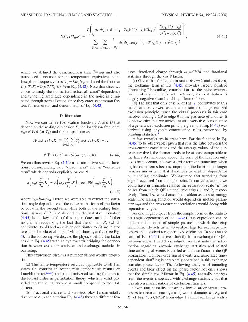
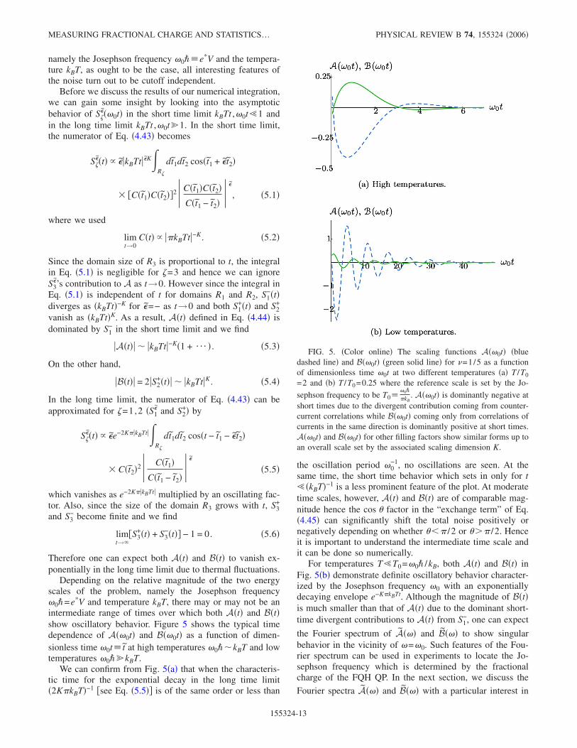
Depending on the relative magnitude of the two energyscales of the problem, namely the Josephson frequency�0�=e*V and temperature kBT, there may or may not be anintermediate range of times over which both A�t� and B�t�show oscillatory behavior. Figure 5 shows the typical timedependence of A��0t� and B��0t� as a function of dimen-sionless time �0t� t at high temperatures �0��kBT and lowtemperatures �0��kBT.

We can confirm from Fig. 5�a� that when the characteris-tic time for the exponential decay in the long time limit�2K�kBT�−1 �see Eq. �5.5�� is of the same order or less than

the oscillation period �0−1, no oscillations are seen. At the

same time, the short time behavior which sets in only for t� �kBT�−1 is a less prominent feature of the plot. At moderatetime scales, however, A�t� and B�t� are of comparable mag-nitude hence the cos � factor in the “exchange term” of Eq.�4.45� can significantly shift the total noise positively ornegatively depending on whether ��� /2 or �� /2. Henceit is important to understand the intermediate time scale andit can be done so numerically.

For temperatures T�T0=�0� /kB, both A�t� and B�t� inFig. 5�b� demonstrate definite oscillatory behavior character-ized by the Josephson frequency �0 with an exponentiallydecaying envelope e−K�kBTt. Although the magnitude of B�t�is much smaller than that of A�t� due to the dominant short-time divergent contributions to A�t� from S1

−, one can expect

the Fourier spectrum of A��� and B��� to show singularbehavior in the vicinity of �=�0. Such features of the Fou-rier spectrum can be used in experiments to locate the Jo-sephson frequency which is determined by the fractionalcharge of the FQH QP. In the next section, we discuss the

Fourier spectra A��� and B��� with a particular interest in

FIG. 5. �Color online� The scaling functions A��0t� �bluedashed line� and B��0t� �green solid line� for �=1/5 as a functionof dimensionless time �0t at two different temperatures �a� T /T0

=2 and �b� T /T0=0.25 where the reference scale is set by the Jo-

sephson frequency to be T0��0�

�kB. A��0t� is dominantly negative at

short times due to the divergent contribution coming from counter-current correlations while B��0t� coming only from correlations ofcurrents in the same direction is dominantly positive at short times.A��0t� and B��0t� for other filling factors show similar forms up toan overall scale set by the associated scaling dimension K.

MEASURING FRACTIONAL CHARGE AND STATISTICS… PHYSICAL REVIEW B 74, 155324 �2006�

155324-13

extracting signatures of fractional statistics and fractionalcharge.

VI. FREQUENCY SPECTRUM S„�…

As with the time dependent noise, it can be seen from Eq.�4.42� that the frequency spectrum of the normalized noise

also gets contributions S�� from different domains R� as the

following:

S��� = �−�

�

dtei�tS�t� � ��=1,3

��=±

S����� + 2 cos �S2

+��� .

�6.1�

Noting the fact that the oscillatory time dependence of allS���t� comes from the factor cos��0�t− t1− �t2�� in Eq. �4.43�

�t��0t�, we can use the identity

cos��0�t − t1 − �t2�� = cos��0t�cos��0�t1 + �t2��

+ sin��0t�sin��0�t1 + �t2�� �6.2�

to factor out oscillatory factors from each S���t� as the follow-

ing:

S���t� � �cos��0t�F���t� + sin��0t�H�

��t�� , �6.3�

where the decaying envelope functions F���t� and H���t� are

defined by

F���t� � ��R�

dt1dt2 cos��0�t1 + �t2��

��C�t − t1�C�t2��2�C�t1�C�t − t2�

C�t1 − t2�C�t�� �, �6.4�

H���t� � ��

R�

dt1dt2 sin��0�t1 + �t2��

��C�t − t1�C�t2��2�C�t1�C�t − t2�

C�t1 − t2�C�t�� � �6.5�

from Eq. �6.2� and Eq. �4.43�.It is clear from Eq. �6.3� that S����

� is a convolution of anoscillating part and the envelopes which we may simplycompute. Thus we have

S����� �

1

2�F���� + �0� + F���� − �0��

+1

2i�H�

��� + �0� + H���� − �0�� , �6.6�

with

F����� = �−�

�

dtF���t�ei�t = 2�0

�

dt cos �tF���t� ,

H����� = �

−�

�

dtH���t�ei�t = 2i�

0

�

dt sin �tH���t� , �6.7�

where we used the fact that F���t� is even in t while H���t� is

odd in t. Hence we can understand the frequency spectrum

by investigating frequency spectra F�����, H����� and super-

posing them with their centers shifted by ±�0. One important

observation to be made in Eq. �6.7� is the fact that F����� is

an even function of � while H����� is an odd function of �.

As we discussed in the previous section �see Eq. �5.5��, S���t�

decays exponentially as e−2K�kBTt in the long time limit�K�kBTt��1 and hence

F���t� � H�

��t� → e−2K�kBTt �6.8�

in the long time limit as well. As a result, the form of F�����is a broadened peak at �=0 with the width of the peak2K�kBT determined by the temperature and the scaling di-

mension of FQH QP. Similarly, H����� takes the form of a

derivative of a peak with the same width. The characteristic

behavior of F����� and H����� is plotted in Fig. 7.

From the definition of the “direct” and “exchange” terms

in Eq. �4.44�, we can express A��� and B��� in terms of

F����� and H����� as

A��� = ��=1,3

��=±

1

2�F����0 + �;T,K� + F����0 − �;T,K��

+ ��=1,3

��=±

1

2i�H�

���0 + �;T,K� − H����0 − �;T,K�� ,

�6.9�

B��� =1

2�F2

+��0 + �;T,K� + F2+��0 − �;T,K��

+1

2i�H2

+��0 + �;T,K� − H2+��0 − �;T,K�� .

�6.10�

In the rest of this section, we use the properties of F����� and

H����� to understand and discuss A��� and B��� in two fre-

quency regimes of interest: low frequency ���0 and nearJosephson frequency ���0.

For ���0, both A��� and B��� collect tail ends of

shifted F����� and H�����. Naturally, they show white noise

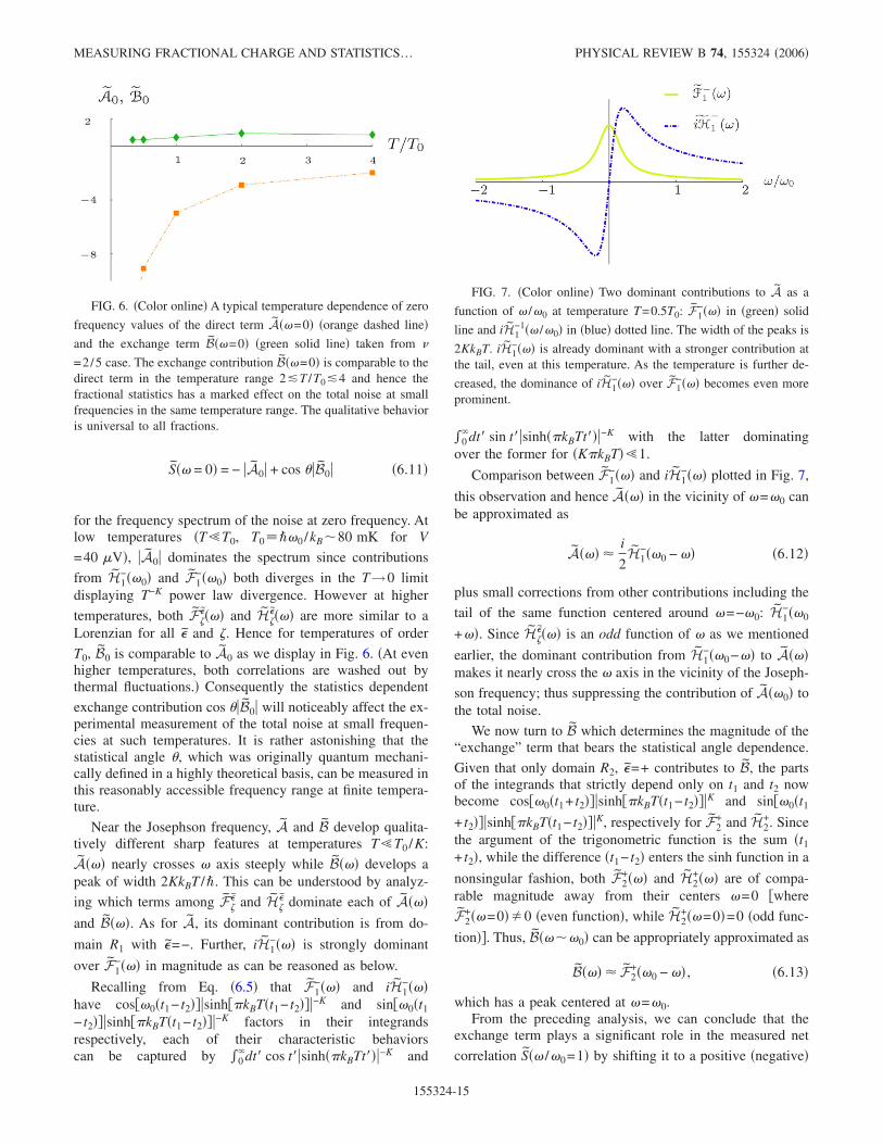
behavior and hence we focus on zero frequency values

A��=0��A0 and B��=0�� B0 which depend only on the

temperature �see Fig. 6�. The direct term A0 is negative dueto its dominant contributions coming from �=− processes indomain R1 with the opposite orientation of the currents as

illustrated in case O of Fig. 3. On the other hand, B0 ispositive as it only involves case S��= + � from domain R2. Asa result, Eq. �4.45� translates to

KIM et al. PHYSICAL REVIEW B 74, 155324 �2006�

155324-14

S�� = 0� = − �A0� + cos ��B0� �6.11�

for the frequency spectrum of the noise at zero frequency. Atlow temperatures �T�T0, T0���0 /kB�80 mK for V

=40 �V�, �A0� dominates the spectrum since contributions

from H1−��0� and F1

−��0� both diverges in the T→0 limitdisplaying T−K power law divergence. However at higher

temperatures, both F����� and H����� are more similar to a

Lorenzian for all � and �. Hence for temperatures of order

T0, B0 is comparable to A0 as we display in Fig. 6. �At evenhigher temperatures, both correlations are washed out bythermal fluctuations.� Consequently the statistics dependent

exchange contribution cos ��B0� will noticeably affect the ex-perimental measurement of the total noise at small frequen-cies at such temperatures. It is rather astonishing that thestatistical angle �, which was originally quantum mechani-cally defined in a highly theoretical basis, can be measured inthis reasonably accessible frequency range at finite tempera-ture.

Near the Josephson frequency, A and B develop qualita-tively different sharp features at temperatures T�T0 /K:

A��� nearly crosses � axis steeply while B��� develops apeak of width 2KkBT /�. This can be understood by analyz-

ing which terms among F�� and H�� dominate each of A���

and B���. As for A, its dominant contribution is from do-

main R1 with �=−. Further, iH1−��� is strongly dominant

over F1−��� in magnitude as can be reasoned as below.

Recalling from Eq. �6.5� that F1−��� and iH1

−���have cos��0�t1− t2���sinh��kBT�t1− t2���−K and sin��0�t1

− t2���sinh��kBT�t1− t2���−K factors in their integrandsrespectively, each of their characteristic behaviorscan be captured by �0

�dt� cos t��sinh��kBTt���−K and

�0�dt� sin t��sinh��kBTt���−K with the latter dominating

over the former for �K�kBT��1.

Comparison between F1−��� and iH1

−��� plotted in Fig. 7,

this observation and hence A��� in the vicinity of �=�0 canbe approximated as

A��� �i

2H1

−��0 − �� �6.12�

plus small corrections from other contributions including the

tail of the same function centered around �=−�0: H1−��0

+��. Since H����� is an odd function of � as we mentioned

earlier, the dominant contribution from H1−��0−�� to A���

makes it nearly cross the � axis in the vicinity of the Joseph-

son frequency; thus suppressing the contribution of A��0� tothe total noise.

We now turn to B which determines the magnitude of the“exchange” term that bears the statistical angle dependence.

Given that only domain R2, �=+ contributes to B, the partsof the integrands that strictly depend only on t1 and t2 nowbecome cos��0�t1+ t2���sinh��kBT�t1− t2���K and sin��0�t1

+ t2���sinh��kBT�t1− t2���K, respectively for F2+ and H2

+. Sincethe argument of the trigonometric function is the sum �t1

+ t2�, while the difference �t1− t2� enters the sinh function in a

nonsingular fashion, both F2+��� and H2

+��� are of compa-rable magnitude away from their centers �=0 �where

F2+��=0��0 �even function�, while H2

+��=0�=0 �odd func-

tion��. Thus, B����0� can be appropriately approximated as

B��� � F2+��0 − �� , �6.13�

which has a peak centered at �=�0.From the preceding analysis, we can conclude that the

exchange term plays a significant role in the measured net

correlation S�� /�0=1� by shifting it to a positive �negative�

FIG. 6. �Color online� A typical temperature dependence of zero

frequency values of the direct term A��=0� �orange dashed line�and the exchange term B��=0� �green solid line� taken from �

=2/5 case. The exchange contribution B��=0� is comparable to thedirect term in the temperature range 2 T /T0 4 and hence thefractional statistics has a marked effect on the total noise at smallfrequencies in the same temperature range. The qualitative behavioris universal to all fractions.

FIG. 7. �Color online� Two dominant contributions to A as a

function of � /�0 at temperature T=0.5T0: F1−��� in �green� solid

line and iH1−1�� /�0� in �blue� dotted line. The width of the peaks is

2KkBT. iH1−��� is already dominant with a stronger contribution at

the tail, even at this temperature. As the temperature is further de-

creased, the dominance of iH1−��� over F1

−��� becomes even moreprominent.

MEASURING FRACTIONAL CHARGE AND STATISTICS… PHYSICAL REVIEW B 74, 155324 �2006�

155324-15

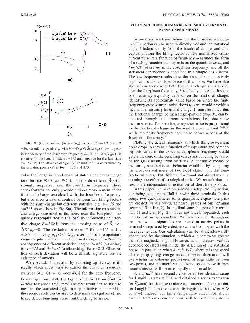
value for Laughlin �non-Laughlin� states since the exchangeterm has cos �0 �cos ��0�, and the direct term A��� isstrongly suppressed near the Josephson frequency. Thesesharp features not only provide a direct measurement of thefractional charge associated with the Josephson frequency,but also allow a natural contrast between two filling factorswith the same charge but different statistics, e.g., �=1/5 and�=2/5, as we show in Fig. 8�a�. The information on statisticsand charge contained in the noise near the Josephson fre-quency is recapitulated in Fig. 8�b� by introducing an effec-

tive charge e��� /V from the crossing point of S, i.e.,

S�� /�0�=0. The deviation between e for �=1/5 and �=2/5—satisfying e1/5�e*� e2/5 over a broad temperaturerange despite their common fractional charge e*=e /5—is aconsequence of different statistical angles �=� /5 �bunching�for �=1/5 and �=3� /5 �antibunching� for �=2/5. Observa-tion of such deviation will be a definite signature for theexistence of anyons.

We conclude this section by summing up the two mainresults which show ways to extract the effect of fractional

statistics S��=0�=−�A0�+cos ��B0� for the zero frequency

Fourier spectrum plotted in Fig. 6; e* defined from S��� for� near Josephson frequency. The first result can be used tomeasure the statistical angle in a quantitative manner whilethe second result can be used to determine the sgn�cos �� andhence detect bunching versus antibunching behavior.

VII. CONCLUDING REMARKS AND MULTI-TERMINALNOISE EXPERIMENTS

In summary, we have shown that the cross-current noisein a T junction can be used to directly measure the statisticalangle � independently from the fractional charge, and con-ceptually, from the filling factor �. The normalized cross-current noise as a function of frequency � assumes the formof a scaling function that depends on the quantities � /�0 and��0 /kT, where �0 is the Josephson frequency, and all thestatistical dependence is contained in a simple cos � factor.The low frequency results show that there is a quantitativelysignificant statistics dependence of this noise. We have alsoshown how to measure both fractional charge and statisticsnear the Josephson frequency. Specifically, since the Joseph-son frequency explicitly depends on the fractional charge,identifying its approximate value based on where the finitefrequency cross-current noise drops to zero would provide ameans of measuring fractional charge. It must be noted thatthe fractional charge, being a single-particle property, can bedetected through autocurrent correlations, i.e., shot noisemeasurements. The zero frequency shot noise is proportionalto the fractional charge in the weak tunneling limit12–14,31

while the finite frequency shot noise shows a peak at theJosephson frequency.25

Plotting the actual frequency at which the cross-currentnoise drops to zero as a function of temperature and compar-ing this value to the expected Josephson frequency wouldgive a measure of the bunching versus antibunching behaviorof the QP’s arising from statistics. A definitive means ofmeasuring such statistical behavior would be by comparingthe cross-current noise of two FQH states with the samefractional charge but different fractional statistics, thus pin-pointing the effect of topological order. We remark that ourresults are independent of nonuniversal short time physics.

In this paper, we have considered a setup, the T junction,consisting of quantum Hall bar with three terminals. In thissetup, two quasiparticles �or a quasiparticle-quasihole pair�are created �or destroyed� at nearby places of one terminal�terminal 0 in Fig. 2�. In the final state the two other termi-nals �1 and 2 in Fig. 2�, which are widely separated, eachdetects just one quasiparticle. We have assumed throughoutthat the two quasiparticles are created at nearby points interminal 0 separated by a distance a small compared with themagnetic length. Our calculation can be straightforwardlygeneralized for the situation in which a is somewhat greaterthan the magnetic length. However, as a increases, variousdecoherence effects will hinder the detection of the statisticalphase. In particular, when a!v� /kBT, where v is the speedof the propagating charge mode, thermal fluctuation willoverwhelm the coherent propagation of edge state betweentwo points, and the interference effects associated with frac-tional statistics will become rapidly unobservable.

Safi et al.22 have recently considered the identical setupfor Laughlin states at T=0 and obtained a series expression

for S��=0� for the case O alone as a function of � �note thatfor Laughlin states one cannot distinguish � from K or e* /eor � /��. Indeed, our finite temperature calculation showsthat the total cross current noise will be completely domi-

FIG. 8. �Color online� �a� S�� /�0� for �=1/5 and 2/5 for T

=20, 40 mK, respectively, with V�40 �V. S�� /�0� shows a peak

in the vicinity of the Josephson frequency �0. At �0, S�� /�0=1� ispositive for the Laughlin state �=1/5 and negative for the Jain state�=2/5. �b� The effective charge e�T� in units of e is determined bythe crossing points of �a� for �=1/5 and 2/5.

KIM et al. PHYSICAL REVIEW B 74, 155324 �2006�

155324-16

nated by case O as T→0 which was the case of interest inRef. 22. However, our study also shows that, at finite tem-peratures, case S brings in an explicit statistics dependence inthe form of cos � which can be distinguished from the effectof the fractional charge and the scaling dimension for non-Laughlin states. Furthermore, even at relatively low tempera-ture at which most noise experiments involving QH systemstake place �see below�, this statistics dependent contributionwas found to be of comparable magnitude as the statisticsindependent contribution. It is rather encouraging to find thata purely quantum mechanical property such as statistics canin principle be observed in our setup at nonzero tempera-tures. In fact it is precisely the finite temperature that assistsprocesses that are sensitive to statistics. A closely relatedsetup is the four terminal case studied �only for Laughlinstates at T=0� by Vishveshwara in Ref. 29, where the crosscurrent noise at equal times t=0 was calculated for the con-tribution that involves all four terminals. We should note,however, that even in this case, an actual measurement of thecross-correlation will have contributions from correlation be-tween three of the four terminals which is precisely S�t� wehave calculated here. A number of interesting interferometershave been proposed to detect fractional statistics,32–35 noneof which has yet been realized experimentally, except possi-bly for the recent experiments of Refs. 36–38. Theoreticalschemes to measure non-Abelian statistics have also beenproposed.39,40

Here we have presented the calculation using the edgestate theory constructed by Lopez and Fradkin for Jainstates.17 However, as long as one can limit oneself to a singlepropagating mode by either choosing the most relevant modeof hierarchical picture �see below� or by using Lopez-Fradkin picture which only has one propagating mode bydesign, the theory presented here is applicable and couldindeed be used to compare predictions from different de-scriptions.

For the T-junction setup studied here, the hierarchical pic-ture would imply multiple propagating edge modes for non-Laughlin states. In Ref. 10, Wen derived the effective theoryfor edge states of hierarchical FQH states followingHaldanes hierarchical construction.41 According to the hier-archical theory, the �=2/5 FQH state is generated by thecondensation of quasiparticles on top of the �=1/3 FQHstate. Thus the 2/5 state contains two components of incom-pressible fluids. If we consider a special edge potential suchthat the FQH state consists of two droplets, then in this pic-ture, one is the electron condensate with a filling fraction�1=1/3 and radius r1, and the other is the quasiparticle con-densate �on top of the 1/3 state� with a filling fraction�2=1/15 �note 1/3+1/15=2/5� and radius r2�r1.Recently, one of us used this picture42 to account for thesuperperiod Aharonov-Bohm oscillations observed in recentexperiments,36–38 where the smooth edge potential could in-deed have created two droplet situation. On the other hand, ifthe edge is sharply defined so that there can be direct tunnel-ing between descendant states �2/5 state, for example�, it isreasonable to consider the tunneling current being domi-nantly carried by the mode which has the smallest scalingdimension �that is “most” relevant in the renormalizationgroup sense�. In Wen’s theory, although the primary edge QP

mode carries e*=1/5, � /�=K=3/5, it is actually the QPmode with e*=� /�=K=2/5 that is most relevant,10 which isquite different from the e*=1/5, � /�=3/5, K=1/10 for thecharge mode in Lopez-Fradkin picture. In fact, given that ourcalculation is applicable to alternate pictures which comewith different predictions, an experiment such as the oneproposed here, where the charge and statistics of Jain statequasiparticles can separately be identified, becomes all themore immediate.

Turning to experiments, some recent measurements in aquantum interferometer geometry were interpreted to implyfractional statistics. An effective charge extracted in recentshot noise experiments43 was somewhat larger than the mini-mum quasiparticle charge, suggesting bunching behavior.Observation of Aharonov-Bohm oscillations with a superpe-riod in an antidot36–38 have also been ascribed to statisticaleffects. However, the noise measurements we propose herewill allow for a direct and independent way of measuringboth fractional statistics and charge separately. Low fre-quency prediction have the advantage of yielding quantita-tively significant statistics dependence of the noise. Near theJosephson frequency, our prediction has the strength of prob-ing both charge and statistics simultaneously. The geometryproposed and the required experimental conditions are allvery much within current capabilities. The T-junction setupis reminiscent of the multilead geometry employed in effec-tive charge measurement, though, the issue of whether or notthe fabricated T junction would form a single point contactwould be relevant. Typical parameters used in noiseexperiments14,43 are bias voltages of 10–150 �V �corre-sponding to a Josephson frequency �0�1 GHz�, and tem-peratures of 10–100 mK. These parameters access the ratiosof T /T0 shown here, making our proposal plausible. The pa-rameter regime in which the perturbative results for cross-current correlations are valid depends on the interedge tun-neling amplitude and consequently on fabrication. Thecondition �on applied voltage and temperature� for remainingin this regime is that the ratio between tunneling current andmaximum edge state current �e2V /h be small, i.e., of order0.1.

A definitive measurement of anyonic statistics, such as theone proposed here, would be one of the first instances ofexperimentally establishing the existence of topologicalorder.10,19 Employing topological order has recently emergedas a possible route to decoherence free quantumcomputing.44 Clear signatures of fractional statistics wouldmark the very first steps towards bringing some of thesefascinating ideas to life.

ACKNOWLEDGMENTS

This work was supported in part by the National ScienceFoundation through Grant Nos. DMR 04-42537 �E.K., M.L.,E.F.�, DOE-MRL DEFG02-91-ER45439 �S.V.�, by the Re-search Board of the University of Illinois �E.F., M.L.�, andby a Stanford Institute for Theoretical Physics �E.K.�. Wethank F.D.M. Haldane for illuminating discussions regardingexclusion statistics in the setup of this paper and C. Chamonfor many helpful comments �particularly on Klein factors�.

MEASURING FRACTIONAL CHARGE AND STATISTICS… PHYSICAL REVIEW B 74, 155324 �2006�

155324-17

We also thank M. Heiblum and C. Marcus for discussions onnoise experiments. We thank E. Ardonne for many helpfuldiscussions.

APPENDIX A: CHIRAL AND NONCHIRAL BOSONCOMMUTATION RELATIONS AND CORRELATION

FUNCTIONS

In this appendix we quantize the chiral boson theory andcalculate its correlation function. We also extend this calcu-lation to the case of a neutral topological field that is non-propagating.

The Lagrangian density for a left/right moving free mass-less chiral boson field �±�x±vt� propagating with speed v is

L± =g

4��x�±�±�t�± − v�x�±� �A1�

with the corresponding action S0=�d2rL, where r�= �x , t� andg is a positive real parameter. Notice that the Lagrangian isinvariant under an arbitrary overall shift of the field �±, i.e.,

L±��±�r��� = L±��±�r�� + �� �A2�

with an arbitrary constant �. Hence L± is independent of thezero mode of �±.

Correct quantization of these chiral bosons can beachieved by the following equal time commutation relations

��±�x,t�, ±g

4��x��±�x�,t�� =

1

2i �x − x�� , �A3�

where the factor of 12 comes from the fact that �± are non-

local fields with respect to the nonchiral boson ���−+�+occupying only half the phase space of �. The nonchiralboson � is a true local field and it can be quantized in theusual way. We will find below that Eq. �A3� is indeed thecorrect commutation relations consistent with the commuta-tion relations of nonchiral boson. To find the nonchiral bosonLagrangian using a path integral, we need another �dual�nonchiral bosonic field � to change the basis from �− and �+to � and �. Hence we define

�� �− − �+ �A4�

and write �± in terms of � and � as the following:

�+ =1

2�� − ��, �− =

1

2�� + �� . �A5�

Then the total Lagrangian for two fields can be written interms of � and � as

L+ + L− = −g

8���x��t� + �x��t� + v��x��2 + v��x��2�

�A6�

and the path integral for two chiral fields can be written as apath integral for two nonchiral fields to give

Z =� D�−� D�+ei�d2r�L++L−�

=� D�� D�e−i�g/8���d2r�v��x��2+2�t��x�+v��x��2�. �A7�

Now we can integrate � out from the above equation

Z =� D�ei�d2r�g/8���1/v��t��2−v��x��2� �A8�

to obtain the Lagrangian for the nonchiral field �

L��� =g

8��1

v��t��2 − v��x��2� . �A9�

We can find the canonical conjugate of �, "� in the usualway to be

"� � L �t�

=1

v

g

4��t� �A10�

with the equal time commutation relation

���x�,"��x��� = i �x − x�� . �A11�

However, since �=�−�x−vt�+�+�x+vt�

�t� = �t��− + �+� = − v�x��− + �+� = − v�x� �A12�

which means �x� is proportional to the canonical conjugate"�:

"� = −g

4��x� �A13�

and hence Eq. �A11� can be rewritten as

���x�,�x���x��� = − i4�

g �x − x�� . �A14�

From Eqs. �A5� and �A14� one can check that Eq. �A3� in-deed is the correct way of quantizing the chiral modes.

Now integrating both sides of Eq. �A3� withrespect to x�−x and noting that �x�−x��±�x� ,�±�x���= ��±�x� ,�x��±�x���− ��x�±�x� ,�±�x���, one finds the follow-ing equal time commutation relations for left/right movingbosons �±

��+�x�,�+�x��� = − i�

gsgn�x − x�� ,

��−�x�,�−�x��� = i�

gsgn�x − x�� . �A15�

To calculate the chiral boson propagator, we first define agenerating functional

�Z�a� =� D�±ei�d2r�L±��±��+a�±�

= Z�0�e−�1/2��d2r�d2r�a�r�M±−1�r−r��a�r��, �A16�

where we defined the differential operator associated withthe Lagrangian L±

KIM et al. PHYSICAL REVIEW B 74, 155324 �2006�

155324-18

M± � ig

2��x�±�t − v�x� . �A17�

Now the propagator is nothing but the inverse of M since

G±�r� − r��� = �±�r���±�r��� = − ln Z�a� a�r�� a�r���

a=0

= M±−1�r� − r��� , �A18�

and can be calculated using a Fourier transformation with theproper epsilon prescription for a time ordered propagator�substituting � with �+ i� sgn��� in the limit �→0+�:

G±�r�� =� dkd�

�2��2

2�

ig

ei�kx−�t�

ik�#i�� + i� sgn���� − ivk�

= i� dkd�

2�

1

g

e−i��t±kx�

k�� + i� sgn��� − vk�

=1

g� dk

k�e−ik�vt±x�−k�0$�k�$�t�

− eik�vt±x�+k�0$�− k�$�− t�� . �A19�

Here we introduced a UV �short distance� cutoff �0 and usedthe fact that the � contour integral has to be closed in thelower �upper� half plane for t0 �t�0� and sgn���=sgn�k� near the pole at �=vk. Notice that the left �right�moving propagator G+ �G−� indeed depends only on vt+x�vt−x�, i.e., �±�x , t�=�±�vt±x�. It is clear from Eq. �A19�that G�r� has a logarithmic divergence in the small k �IR�limit. However, one can define a finite quantity by subtract-ing the equal position propagator G�0�, which also has alogarithmic divergence, and obtain the following:

G±�r�� � G±�r�� − G±�0�

=1

g� dk

k��e−ik�vt±x�−k�0 − 1�$�k�$�t�

− �eik�vt±x�+k�0 − 1�$�− k�$�− t��

= −1

gln� �0 + i sgn�t��vt ± x�

�0� . �A20�

At finite temperatures T, the regulated and time orderedpropagator can be calculated from Eq. �A20� via conformalmapping to take the following form:

G±�x�,t� = −1

gln�

�

��0

sin���0

�+ i sgn�t�

�

��vt ± x��� ,

�A21�

where �=1/ �kBT� is the inverse temperature with kB beingthe Boltzmann constant.

In the nonpropagating limit of vN→0+, Eq. �A1� becomesthe Lagrangian for a topological field17,45 as the following:

LN =gN

4��x�N�t�N, �A22�

where gN can be either positive or negative real number. LNis still invariant under an arbitrary overall shift of the topo-logical field �N and the propagator for the topological fieldcan be calculated in the similar way as for the chiral field:

T�N�r���N�0� = −i

gN� dkd�

2�

ei�kx−�t�

k�

= −i

gN

1

2��− i�$�t� + i�$�− t��

��i�$�x� − i�$�− x��

= −i

gN

�

2sgn�t�sgn�x�

= limvN→0+

i

gN

�

2sgn�t�sgn�vNt + x� ,

�A23�

where the limit should be taken at the end of any calculationthat uses �N�r���N�0�.

APPENDIX B: CONTOUR ORDERED (KELDYSH)PROPAGATORS FOR CHIRAL BOSONS

Here we derive the contour ordered Green functions forchiral bosons described by the Lagrangian �A1� and topo-logical modes described by Eq. �A22�. Time ordered propa-gator can be thought of as a sum of two terms depending onthe sign of �t− t��:

T��x,t���x�,t�� =$�t − t����x,t���x�,t��

+$�t� − t���x�,t����x,t� . �B1�

In the same way, a contour ordered propagator is determinedby the order in which different times appear on the contoursketched in Fig. 9

G�,���x − x�,t − t�� = TK��x,t����x�,t����

� ���x,t����x�,t���� for t�Kt���,

��x�,t������x,t�� for t���Kt�,�

�B2�

where we used the expression tKt� to denote t appearinglater than t� in the contour. Clearly when both times occur in

FIG. 9. The Keldysh contour from t=−� to t=� along the for-ward branch ��= + �, and back to t=−� along the backward branch��=−�.

MEASURING FRACTIONAL CHARGE AND STATISTICS… PHYSICAL REVIEW B 74, 155324 �2006�

155324-19

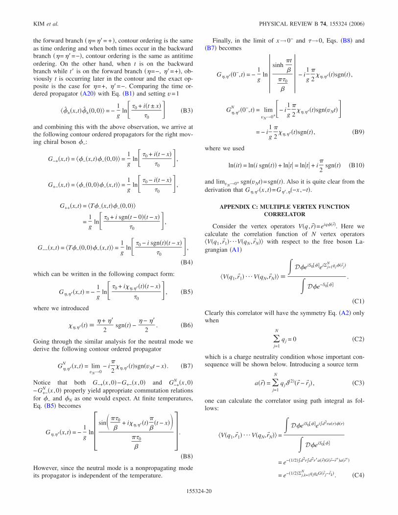
the forward branch ��=��= + �, contour ordering is the sameas time ordering and when both times occur in the backwardbranch ��=��=−�, contour ordering is the same as antitimeordering. On the other hand, when t is on the backwardbranch while t� is on the forward branch ��=−, ��=+�, ob-viously t is occurring later in the contour and the exact op-posite is the case for �=+, ��=−. Comparing the time or-dered propagator �A20� with Eq. �B1� and setting v=1

�±�x,t��±�0,0� = −1

gln� �0 + i�t ± x�

�0� �B3�

and combining this with the above observation, we arrive atthe following contour ordered propagators for the right mov-ing chiral boson �−:

G−+�x,t� = �−�x,t��−�0,0� =1

gln� �0 + i�t − x�

�0� ,

G+−�x,t� = �−�0,0��−�x,t� =1

gln� �0 − i�t − x�

�0� ,

G++�x,t� = T�−�x,t��−�0,0�

=1

gln� �0 + i sgn�t − 0��t − x�

�0� ,

G−−�x,t� = T�−�0,0��−�x,t� =1

gln� �0 − i sgn�t��t − x�

�0� ,

�B4�

which can be written in the following compact form:

G�,���x,t� = −1

gln� �0 + i��,���t��t − x�

�0� , �B5�

where we introduced

��,���t� �� + ��

2sgn�t� −

� − ��

2. �B6�

Going through the similar analysis for the neutral mode wederive the following contour ordered propagator

G�,��N �x,t� = lim

vN→0− i�

2��,���t�sgn�vNt − x� . �B7�

Notice that both G−+�x ,0�−G+−�x ,0� and G−+N �x ,0�

−G+−N �x ,0� properly yield appropriate commutation relations

for �− and �N as one would expect. At finite temperatures,Eq. �B5� becomes

G�,���x,t� = −1

gln� sin���0

�+ i��,���t�

�

��t − x��

��0

�� .

�B8�

However, since the neutral mode is a nonpropagating modeits propagator is independent of the temperature.

Finally, in the limit of x→0− and �→0, Eqs. �B8� and�B7� becomes

G�,���0−,t� = −

1

gln� sinh

�t

�

��0

�� − i

1

g

�

2��,���t�sgn�t� ,

G�,��N �0−,t� = lim

vN→0+�− i

1

g

�

2��,���t�sgn�vNt��

= − i1

g

�

2��,���t�sgn�t� , �B9�

where we used

ln�it� = ln�i sgn�t�� + ln�t� = ln�t� + i�

2sgn�t� �B10�

and limvN→0+ sgn�vNt�=sgn�t�. Also it is quite clear from thederivation that G�,���x , t�=G��,��−x ,−t�.

APPENDIX C: MULTIPLE VERTEX FUNCTIONCORRELATOR

Consider the vertex operators V�q ,r��=eiq��r��. Here wecalculate the correlation function of N vertex operatorsV�q1 ,r�1�¯V�qN ,r�N� with respect to the free boson La-grangian �A1�

V�q1,r�1� ¯ V�qN,r�N� �� D�eiS0���ei�j=1

N qj��r�j�

� D�e−S0���

.

�C1�

Clearly this correlator will have the symmetry Eq. �A2� onlywhen

�j=1

N

qj = 0 �C2�

which is a charge neutrality condition whose important con-sequence will be shown below. Introducing a source term

a�r�� = �j=1

N

qj �2��r� − r� j� , �C3�

one can calculate the correlator using path integral as fol-lows:

V�q1,r�1� ¯ V�qN,r�N� =� D�eiS0���ei�d2ra�r���r�

� D�eiS0���

= e−�1/2��d2r�d2r�a�r��G�r�−r���a�r���

= e−�1/2��j,k=1N qjqkG�r�j−r�k�. �C4�

KIM et al. PHYSICAL REVIEW B 74, 155324 �2006�

155324-20

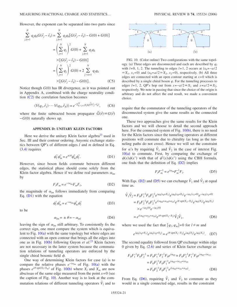
However, the exponent can be separated into two parts since

�j,k=1

N

qjqkG�r� j − r�k� = �j,k=1

N

qjqk�G�r� j − r�k� − G�0� + G�0��

= ��j=1

N

qj�2

G�0� + �j,k=1

N

qjqk

��G�r� j − r�k� − G�0��

= ��j=1

N

qj�2

G�0� + 2 �jk=1

N

qjqk

��G�r� j − r�k� − G�0�� . �C5�

Notice though G�0� has IR divergence, as it was pointed outin Appendix A, combined with the charge neutrality condi-tion �C2� the correlation function becomes

V�q1,r�1� ¯ V�qN,r�N� = e−�kj=1N qjqkG�r�j−r�k�, �C6�

where the finite subtracted boson propagator G�r���G�r��−G�0� naturally shows up.

APPENDIX D: UNITARY KLEIN FACTORS

Here we derive the unitary Klein factor algebra23 used inSec. III and their contour ordering. Anyonic exchange statis-tics between QP’s of different edges l and m defined in Eq.�3.4� requires

l†m

† = e±i�m†l

†. �D1�

However, since boson fields commute between differentedges, the statistical phase should come solely from theKlein factor algebra. Hence if we define real parameters �lmby

FlFm = e−i�lmFmFl, �D2�

the magnitude of �lm follows immediately from comparingEq. �D1� with the equation

l†m

† = e−i�lmm†l

† �D3�

to be

�lm = ± � = − �ml �D4�

leaving the sign of �lm still arbitrary. To consistently fix thecorrect sign, one must compare the system which is equiva-lent to Fig. 10�a� with the same topology but where edges areconnected with an open contour that brings all the edges intoone as in Fig. 10�b� following Guyon et al.23 Klein factorsare not necessary in the latter system because the commuta-tion relations of tunneling operators are enforced by thesingle chiral bosonic field �.

One way of determining Klein factors for case �a� is tocompare the relative phases e−i�lm of Fig. 10�a� with thephases ei� sgn�Xl−Xm� of Fig. 10�b� where Xl and Xm are nowabscissas of the same edge measured from the point x=0 �seethe caption of Fig. 10�. Another way is to look at the com-

mutation relations of different tunneling operators Vl and to

require that the commutator of the tunneling operators of thedisconnected system give the same results as the connectedone.

These two approaches give the same results for the Kleinfactors and we will choose to detail the second approachhere. For the connected system of Fig. 10�b�, there is no needfor the Klein factors since the tunneling operators at differentpositions will commute due to chirality �as long as the tun-neling paths do not cross�. Hence we will set the constraint

for �’s by requiring V1 and V2 in the case of interest Fig.10�a� to commute. First, by comparing the exchange of�x��x�� with that of †�x��x�� using the CBH formula,one finds that the definition of Eq. �D2� implies

FlFm−1 = ei�lmFm

−1Fl. �D5�

With Eqs. �D2� and �D5� we can exchange V1 and V2 at equaltime as.

V1V2 = F0F1−1F0F2

−1ei�0�x0=X1�ei�0�x0=X2�e−i�1�x1=0�e−i�2�x2=0�

= F0F2−1F0F2

−1ei��02+�10+�21�ei� sgn�X1−X2�ei�0�X2�ei�0�X1�

�e−i�2�0�e−i�1�0�

= ei��02+�21+�10�ei� sgn�X1−X2�V2V1, �D6�

where we used the fact that ��l ,�m�=0 for l�m and

ei�0�x0=X1�ei�0�x0=X2� = ei� sgn�X1−X2�ei�0�X2�ei�0�X1�. �D7�

The second equality followed from QP exchange within edge0 given by Eq. �2.6� and series of Klein factor exchange as

F0F1−1F0F2

−1 = F0F1−1F2

−1F0ei�02 = F0F2−1F1

−1F0ei�02−i�12

= F0F2−1F0F1

−1ei�02−i�12+i�10

= F0F2−1F0F1

−1ei��02+�21+�10�. �D8�

From Eq. �D6�, requiring V1 and V2 to commute as theywould in a single connected edge, results in the constraint

FIG. 10. �Color online� Two configurations with the same topol-ogy. �a� Three edges are disconnected and each are described by �l

with l=0, 1, 2. The tunneling to edges l=1, 2 occurs at �x0=−a /2�X1, x1=0� and �x0=a /2�X2, x2=0�, respectively. �b� All threeedges are connected with an open contour starting at x=0 which isdescribed by a single chiral boson �. For the tunneling processes toedges l=1, 2, QP’s hop out from x=−a /2�X1 and x=a /2�X2,respectively. We note in passing that since the choice of the origin isarbitrary and do not affect the end result, we made a convenientchoice.

MEASURING FRACTIONAL CHARGE AND STATISTICS… PHYSICAL REVIEW B 74, 155324 �2006�

155324-21

�02 + �21 + �10 + � sgn�X1 − X2� = 0, �D9�

which allows us to define �02=�21=−�10=� since X2−X1=a0 �see the caption of Fig. 10�. Further we can conclude

F0F1−1F0F2

−1 = F0F2−1F0F1

−1ei�. �D10�

Now we determine the contour ordered Klein factor“propagator” TK�F0F1

−1���t���F0F2−1����t����0 based on Eq.

�D10�. We first note contour ordering means that �F0F1−1���t��

and �F0F2−1����t���� need to be exchanged whenever t���

Kt�, i.e.,

TK�F0F1−1���t���F0F2

−1����t����0

= ��F0F1−1���t���F0F2

−1����t���� for t�Kt���,

�F0F2−1����t�����F0F1

−1���t�� for t���Kt�.��D11�

From Eq. �D10�, it is clear that a consistent way ofdefining the contour ordered propagator is to assign arelative phase factor of e−i� sgn�X1−X2� between t���Kt�

case �in which the Klein factors need to be exchanged forcontour ordering� and t�Kt��� case �in which no exchange

is neccesary�. Further in order for TKV1�t��V2�t����= TKV2�t����V1�t�� to hold, which would be the case for theconnected edge and which connects us back to the basis forthe derivation of Eq. �D10�, we require

TK�F0F1−1���t���F0F2

−1����t����

= TK�F0F2−1����t�����F0F1

−1���t�� . �D12�

This last requirement can be satisfied by assigning half of therelative phase factor e−i� sgn�X1−X2� to each case of Eq. �D11�and we arrive at the following form:

TK�F0F1−1���t���F0F2

−1����t����0

= ei�����/2�sgn�X1−X2���,���t−t�� = e−i�����/2���,���t−t��,

�D13�

where we used the definition of ��,���t− t�� introducedfor the contour ordered propagator of chiral bosons inEq. �B6�.

1 J. Leinaas and J. Myerheim, Nuovo Cimento Soc. Ital. Fis., B 37,1 �1977�.

2 F. Wilczek, Phys. Rev. Lett. 48, 1144 �1982�.3 D. C. Tsui, H. L. Störmer, and A. C. Gossard, Phys. Rev. Lett.

48, 1559 �1982�.4 R. B. Laughlin, Phys. Rev. Lett. 50, 1395 �1983�.5 D. Arovas, J. R. Schrieffer, and F. Wilczek, Phys. Rev. Lett. 53,

722 �1984�.6 B. I. Halperin, Phys. Rev. Lett. 52, 1583 �1984�.7 F. D. M. Haldane, Phys. Rev. Lett. 67, 937 �1991�.8 R. A. J. van Elburg and K. Schoutens, Phys. Rev. B 58, 15704

�1998�.9 X. G. Wen and Q. Niu, Phys. Rev. B 41, 9377 �1990�.

10 X. G. Wen, Am. J. Optom. Physiol. Opt. 44, 405 �1995�.11 V. J. Goldman and B. Su, Science 267, 1010 �1995�.12 R. de Picciotto, M. Reznikov, M. Heiblum, V. Umansky, G. Bu-

nin, and D. Mahalu, Nature �London� 389, 162 �1997�.13 L. Saminadayar, D. C. Glattli, Y. Jin, and B. Etienne, Phys. Rev.

Lett. 79, 2526 �1997�.14 M. Reznikov, R. de Picciotto, T. G. Griffiths, M. Heiblum, and V.

Umansky, Nature �London� 399, 238 �1999�.15 J. K. Jain, Phys. Rev. Lett. 63, 199 �1989�.16 R. Hanbury-Brown and Q. R. Twiss, Nature �London� 177, 27

�1956�.17 A. López and E. Fradkin, Phys. Rev. B 59, 15323 �1999�.18 E.-A. Kim, M. Lawler, S. Vishveshwara, and E. Fradkin, Phys.

Rev. Lett. 95, 176402 �2005�.19 X. G. Wen, Phys. Rev. B 41, 12838 �1990�.20 A. López and E. Fradkin, Phys. Rev. B 44, 5246 �1991�.21 A. Chang, Rev. Mod. Phys. 75, 1449 �2003�.22 I. Safi, P. Devillard, and T. Martin, Phys. Rev. Lett. 86, 4628

�2001�.

23 R. Guyon, P. Devillard, T. Martin, and I. Safi, Phys. Rev. B 65,153304 �2002�.

24 C. de C. Chamon, D. E. Freed, and X. G. Wen, Phys. Rev. B 51,2363 �1995�.

25 C. de C. Chamon, D. E. Freed, and X. G. Wen, Phys. Rev. B 53,4033 �1996�.

26 L. V. Keldysh, Zh. Eksp. Teor. Fiz. 47, 1515 �1964� �Sov. Phys.JETP 20, 1018 �1965��.

27 L. P. Kadanoff and G. Baym, Quantum Statistical Mechanics�Benjamin, New York, 1962�.

28 J. Rammer and H. Smith, Rev. Mod. Phys. 58, 323 �1986�.29 S. Vishveshwara, Phys. Rev. Lett. 91, 196803 �2003�.30 S. C. Zhang, T. H. Hansson, and S. Kivelson, Phys. Rev. Lett. 62,

82 �1989�.31 C. L. Kane and M. P. A. Fisher, Phys. Rev. Lett. 68, 1220 �1992�;

72, 724 �1994�.32 J. K. Jain, S. A. Kivelson, and D. J. Thouless, Phys. Rev. Lett. 71,

3003 �1993�.33 C. de C. Chamon, D. E. Freed, S. A. Kivelson, S. L. Sondhi, and

X. G. Wen, Phys. Rev. B 55, 2331 �1997�.34 C. L. Kane, Phys. Rev. Lett. 90, 226802 �2003�.35 K. T. Law, D. E. Feldman, and Y. Gefen Phys. Rev. B 74, 045319

�2006�.36 F. E. Camino, W. Zhou, and V. J. Goldman, Phys. Rev. Lett. 95,

246802 �2005�.37 F. E. Camino, W. Xhou, and V. J. Goldman, cond-mat/0510764

�unpublished�.38 W. Zhou, F. E. Camino, and V. J. Goldman, cond-mat/01512329

�unpublished�.39 E. Fradkin, C. Nayak, A. Tsvelik, and F. Wilczek, Nucl. Phys. B

516, 704 �1998�.40 S. Das Sarma, M. Freedman, and C. Nayak, Phys. Rev. Lett. 94,

KIM et al. PHYSICAL REVIEW B 74, 155324 �2006�

155324-22

166802 �2005�.41 F. D. M. Haldane, Phys. Rev. Lett. 51, 605 �1983�.42 E.-A. Kim, cond-mat/0604359 �unpublished�.43 Y. C. Chung, M. Heiblum, and V. Umansky, Phys. Rev. Lett. 91,

216804 �2003�.44 A. Y. Kitaev, Ann. Phys. �N.Y.� 303, 2 �2003�.45 D. H. Lee and X. G. Wen, cond-mat/9809160 �unpublished�.

MEASURING FRACTIONAL CHARGE AND STATISTICS… PHYSICAL REVIEW B 74, 155324 �2006�

155324-23