measurements for estimation of carbon stocks -...
TRANSCRIPT
Measurements for Estimation of Carbon Stocks in Aff orestation and Reforestation Project Activities under the Clean Development Mechanism
A Field Manual

Measurements for Estimation of Carbon Stocks in Afforestation and Reforestation Project Activities under the Clean Development Mechanism
A Field Manual
© 2015 UNFCCC
United Nations Framework Convention on Climate Change
All rights reserved
Unless otherwise noted in this document, content of this publication may be freely reproduced in part or in full, provided the source is
acknowledged.
This document may be referenced as:
UNFCCC (2015). Measurements for Estimation of Carbon Stocks in Afforestation and Reforestation Project Activities under the Clean
Development Mechanism: A Field Manual
For further information please contact:
United Nations Climate Change Secretariat (UNFCCC)
Platz der Vereinten Nationen 1
53113 Bonn, Germany
Telephone +49 (228) 815 10 00
Telefax +49 (228) 815 19 99
Email [email protected]
www.unfccc.int
This publication is available online at <http://www.unfccc.int>
Please report any errors in this publication to [email protected]
Disclaimer
This publication is issued for public information purposes and does not in any way substitute, modify, override or otherwise imply specific
interpretation of official UNFCCC documents.
No warranty is offered that this manual presents all the regulatory requirements that apply to a particular CDM project activity. It is the
responsibility of the user to be aware of the latest requirements applicable to the particular case and the circumstances of their project activity.
While reasonable efforts have been made to ensure the accuracy, correctness and reliability of the information contained in this publication,
the UNFCCC Secretariat and all persons acting for it accept no liability for the accuracy of or inferences from the material contained in this
publication and expressly disclaim liability for any person’s loss arising directly or indirectly from inferences drawn, deductions made, or
acts done in reliance on this publication.
ISBN 978-92-9219-135-1
United NationsFramework Convention on Climate Change
5
Measurements for Estimation of Carbon Stocks
in Afforestation and Reforestation Project Activities under the Clean Development Mechanism
CONTENTS
FOREWORD . . . . . . . . . . . . . . . . . . . . . . . . . . . . . . . . . . . . . . . . . . . . . . . . . . . . . . . 7
PREFACE . . . . . . . . . . . . . . . . . . . . . . . . . . . . . . . . . . . . . . . . . . . . . . . . . . . . . . . . . 8
CHAPTER 1 INTRODUCTION . . . . . . . . . . . . . . . . . . . . . . . . . . . . . . . . . . . . . . . . 10
1.1 Purpose of the manual . . . . . . . . . . . . . . . . . . . . . . . . . . . . . . . . . . . . . . . . . 10
1.2 Scope of the manual . . . . . . . . . . . . . . . . . . . . . . . . . . . . . . . . . . . . . . . . . . . 11
1.3 Structure of the manual . . . . . . . . . . . . . . . . . . . . . . . . . . . . . . . . . . . . . . . . 11
CHAPTER 2 CARBON POOLS IN AFFORESTATION AND REFORESTATION PROJECT ACTIVITIES UNDER THE CLEAN DEVELOPMENT MECHANISM . . . . . . . . . . . .12
2.1 Carbon pools in A/R CDM projects . . . . . . . . . . . . . . . . . . . . . . . . . . . . . . . 12
2.2 Estimation of carbon stocks in carbon pools . . . . . . . . . . . . . . . . . . . . . . . 13
2.2.1 Estimation by default factors . . . . . . . . . . . . . . . . . . . . . . . . . . . . . 13
2.2.2 Estimation by modelling . . . . . . . . . . . . . . . . . . . . . . . . . . . . . . . . . 14
2.2.3 Estimation by measurement . . . . . . . . . . . . . . . . . . . . . . . . . . . . . 14
2.3 Field measurement standards . . . . . . . . . . . . . . . . . . . . . . . . . . . . . . . . . . . 14
CHAPTER 3 MEASUREMENT OF LAND AREAS . . . . . . . . . . . . . . . . . . . . . . . . . 15
3.1 Measurement of land areas . . . . . . . . . . . . . . . . . . . . . . . . . . . . . . . . . . . . . 15
3.2 Land survey by using satellite-based navigation system . . . . . . . . . . . . 15
3.2.1 Basic concepts . . . . . . . . . . . . . . . . . . . . . . . . . . . . . . . . . . . . . . . . . 16
3.2.2 Sources of errors . . . . . . . . . . . . . . . . . . . . . . . . . . . . . . . . . . . . . . . 17
3.2.3 Step-wise method for GPS survey . . . . . . . . . . . . . . . . . . . . . . . . . 17
CHAPTER 4 SAMPLING PLAN . . . . . . . . . . . . . . . . . . . . . . . . . . . . . . . . . . . . . . . 19
4.1 Sampling design . . . . . . . . . . . . . . . . . . . . . . . . . . . . . . . . . . . . . . . . . . . . . . 19
4.2 Sampling plan . . . . . . . . . . . . . . . . . . . . . . . . . . . . . . . . . . . . . . . . . . . . . . . . 19
4.2.1 Stratification . . . . . . . . . . . . . . . . . . . . . . . . . . . . . . . . . . . . . . . . . . . 19
4.2.2 Shape of sample plots . . . . . . . . . . . . . . . . . . . . . . . . . . . . . . . . . . . 21
4.2.3 Size of sample plots . . . . . . . . . . . . . . . . . . . . . . . . . . . . . . . . . . . . . 22
4.2.4 Sample size and allocation . . . . . . . . . . . . . . . . . . . . . . . . . . . . . . . 25
4.2.5 Sample selection . . . . . . . . . . . . . . . . . . . . . . . . . . . . . . . . . . . . . . . 25
United NationsFramework Convention on Climate Change
6
Measurements for Estimation of Carbon Stocks
in Afforestation and Reforestation Project Activities under the Clean Development Mechanism
Contents
CHAPTER 5 CONDUCTING MEASUREMENTS IN SAMPLE PLOTS . . . . . . . . . . 26
5.1 Establishment of fixed area sample plots . . . . . . . . . . . . . . . . . . . . . . . . . 26
5.1.1 Locating sample plot centre . . . . . . . . . . . . . . . . . . . . . . . . . . . . . . 26
5.1.2 Plot boundary demarcation . . . . . . . . . . . . . . . . . . . . . . . . . . . . . . 27
5.1.3 Procedure for plot boundary establishment . . . . . . . . . . . . . . . . 29
5.2 Measurements in fixed area sample plots . . . . . . . . . . . . . . . . . . . . . . . . . 32
5.2.1 Measurement of trees . . . . . . . . . . . . . . . . . . . . . . . . . . . . . . . . . . . 32
5.2.2 Measurement of shrubs . . . . . . . . . . . . . . . . . . . . . . . . . . . . . . . . . 40
5.2.3 Measurement of dead wood . . . . . . . . . . . . . . . . . . . . . . . . . . . . . 40
5.2.4 Measurement of litter . . . . . . . . . . . . . . . . . . . . . . . . . . . . . . . . . . . 41
5.3 Establishment of variable area sample plots . . . . . . . . . . . . . . . . . . . . . . . 41
5.4 Measurements in variable area sample plots . . . . . . . . . . . . . . . . . . . . . . 42
CHAPTER 6 QUALITY ASSURANCE AND QUALITY CONTROL . . . . . . . . . . . . . 44
6.1 QA/QC in forest carbon inventory . . . . . . . . . . . . . . . . . . . . . . . . . . . . . . . 44
6.2 Quality assurance . . . . . . . . . . . . . . . . . . . . . . . . . . . . . . . . . . . . . . . . . . . . . 44
6.2.1 Standardized definitions . . . . . . . . . . . . . . . . . . . . . . . . . . . . . . . . . 44
6.2.2 Standardized procedures . . . . . . . . . . . . . . . . . . . . . . . . . . . . . . . . 47
6.2.3 Documentation . . . . . . . . . . . . . . . . . . . . . . . . . . . . . . . . . . . . . . . . 49
6.2.4 Tolerances and data quality objectives . . . . . . . . . . . . . . . . . . . . . 50
6.2.5 Calibration . . . . . . . . . . . . . . . . . . . . . . . . . . . . . . . . . . . . . . . . . . . . . 51
6.3 Quality control . . . . . . . . . . . . . . . . . . . . . . . . . . . . . . . . . . . . . . . . . . . . . . . . 51
6.3.1 Field inspections . . . . . . . . . . . . . . . . . . . . . . . . . . . . . . . . . . . . . . . 51
6.3.2 Data inspections . . . . . . . . . . . . . . . . . . . . . . . . . . . . . . . . . . . . . . . . 52
APPENDIX A
Worked-out examples . . . . . . . . . . . . . . . . . . . . . . . . . . . . . . . . . . . . . . . . . . . . . . . . 54
APPENDIX B
Conversion tables . . . . . . . . . . . . . . . . . . . . . . . . . . . . . . . . . . . . . . . . . . . . . . . . . . . . 61
APPENDIX C
Glossary of CDM terms . . . . . . . . . . . . . . . . . . . . . . . . . . . . . . . . . . . . . . . . . . . . . . . . 63
APPENDIX D
List of A/R CDM regulatory documents . . . . . . . . . . . . . . . . . . . . . . . . . . . . . . . . . . 67
APPENDIX E
References . . . . . . . . . . . . . . . . . . . . . . . . . . . . . . . . . . . . . . . . . . . . . . . . . . . . . . . . . . 69

United NationsFramework Convention on Climate Change
7
Measurements for Estimation of Carbon Stocks
in Afforestation and Reforestation Project Activities under the Clean Development Mechanism
Foreword
FOREWORD
Forests are one of our planet’s most valuable resources. They are habitats that conserve biodiversity, reduce soil erosion, protect watersheds and sustain indigenous ways of life. They are natural capital that enables economic growth, and they are carbon sinks that mitigate the greenhouse gas emissions that drive climate change. For these reasons, projects that promote afforestation and reforestation are an integral part of the international effort to meet the climate change challenge.
The potential of forests requires careful project planning, implementation and monitoring. However, not all countries have the necessary expertise to effectively bring their forest projects into the Clean Development Mechanism. This manual has been developed as best practice guidance on how to monitor afforestation and reforestation project activities.
Developed by the Sustainable Development Mechanism programme of the UNFCCC with technical support from the CDM Executive Board’s Afforestation and Reforestation Working Group, this manual provides efficient, cost-effective methods for measuring carbon stocks in afforestation and reforestation projects. The goal is to increase CDM access while ensuring environmental integrity through accurate monitoring. I hope this manual helps realize the full potential of forests and helps protect and expand these valuable natural resources into the future.
Christiana Figueres Executive Secretary
United Nations Framework Convention on Climate Change 7 April 2015

United NationsFramework Convention on Climate Change
8
Measurements for Estimation of Carbon Stocks
in Afforestation and Reforestation Project Activities under the Clean Development Mechanism
Preface
PREFACE
Monitoring is a major step for the success of afforestation and reforestation CDM project activities and involves significant costs. The afforestation and reforestation methodologies approved by the Executive Board of the CDM lay down the sampling and statistical estimation methods for estimation of carbon stocks but do not prescribe the field procedures for conducting measurements. While conducting field measurements the project participants are required to follow the commonly accepted principles and practices of forest inventory and forest management in the host country. In many developing countries, particularly where the practice of scientific forest management is not long established, it may be difficult for the project participants to have access to the commonly accepted principles and practices of forest inventory. The present manual intends to fill this gap and facilitate the task of developing standard operating procedures for field measurement of carbon stocks during monitoring of project activities.
The manual brings together in one place the best practice guidance on forest inventory designs and field measurement procedures. The content has been presented in a lucid and accessible manner and includes where necessary step-wise procedures, illustrations and fully worked-out examples.
This manual is not a regulatory document and does not contain any new requirement beyond the requirements prescribed in the approved CDM methodologies and tools. Instead, the manual provides guidance on meeting, in a cost-effective manner, the requirements prescribed in the methodologies and tools. Use of the manual will enhance consistency and quality in monitoring reports of registered project activities apart from facilitating the accessibility of the CDM standards and building capacity of project participants.
I would like to thank the secretariat team for their work leading to this highly accessible and useful publication. Special thanks are due to the members of the Afforestation and Reforestation Working Group whose critical review and valuable inputs resulted in the high quality of the final publication.
John Kilani Director, Sustainable Development Mechanisms programme
United Nations Framework Convention on Climate Change 7 April 2015
United NationsFramework Convention on Climate Change
9
Measurements for Estimation of Carbon Stocks
in Afforestation and Reforestation Project Activities under the Clean Development Mechanism
ABBREVIATIONS AND ACRONYMS
A/R afforestation or reforestation
BAF basal area factor
CDM clean development mechanism
CMP Conference of the Parties serving as the meeting of the Parties to the Kyoto Protocol
dbh diameter at breast height (of a tree)
DOE designated operational entity
DOM dead organic matter
FAO Food and Agriculture Organization (of the United Nations)
GHG greenhouse gas
GIS geographical information system
GNSS global navigation satellite system
GPS global positioning system
IPCC Intergovernmental Panel on Climate Change
LULUCF land use, land-use change and forestry
QA quality assurance
QC quality control
SI International System (Sytème international) of units
SOC soil organic carbon
SSC A/R small-scale afforestation or reforestation
tCER temporary certified emission reduction
UNFCCC United Nations Framework Convention on Climate Change
UNITS OF MEASUREMENT
ha hectare
m metre
t tonne (metric)
tCO2e tonne carbon dioxide equivalent

United NationsFramework Convention on Climate Change
10
Measurements for Estimation of Carbon Stocks
in Afforestation and Reforestation Project Activities under the Clean Development Mechanism
CHAPTER 1 INTRODUCTION
Summary This chapter explains the purpose, the organization and the structure of the manual. It also describes the scope of the manual and points to other clean development mechanism documents relating to afforestation and reforestation project activities which should be consulted along with this manual.
1 .1 PURPOSE OF THE MANUAL
This manual is intended to serve as a guide for conducting measurements for estimation of carbon stocks in afforestation and reforestation (A/R) project activities under the clean development mechanism (CDM).
Approved A/R CDM methodological standards1 provide the methodological requirements for estimation of carbon stocks and changes in carbon stocks in carbon pools, including requirements that apply to measurement-based estimation methods. Measurement-based estimation methods are mainly applied in the monitoring of project activities although such methods can also be applied in the baseline.
A/R CDM methodological standards require that “the commonly accepted principles and practices of forest inventory and forest management in the host country” should be followed while monitoring A/R CDM project activities. Where such principles and practices are not available, the “standard operating procedures (SOPs) and quality assurance/quality control (QA/QC) procedures for inventory operations, including field data collection and data management, shall be identified, recorded and applied”.2 The methodologies further provide that SOPs available from published handbooks, or from the IPCC Good Practice Guidance for Land Use, Land-Use Change and Forestry 20033 (hereinafter referred to as IPCC-GPG-LULUCF 2003), can be used where the commonly accepted principles and practices of forest inventory and forest management in the host country are not available to the project participants.
The present manual aims to assist project participants in meeting the requirements in respect of forest carbon inventory methods suitable for the monitoring of A/R CDM project activities. Where the commonly accepted principles and practices of forest inventory and forest management in the host country are non-existent or are not available to project participants, the guidance and the field procedures provided in this manual can serve as the basis for developing project-specific field measurement SOPs and related QA/QC procedures for the purpose of the monitoring of A/R CDM project activities.
This manual should be used along with other relevant CDM documents, particularly the A/R CDM methodological standards, the CDM Project Standard and the CDM Validation and Verification Standard.4 The manual should also be seen as a
1) In this manual the term ‘A/R CDM methodological standards’ means the approved A/R CDM methodologies and methodological tools. Current versions of the A/R methodological standards can be found on the CDM website at <https://cdm.unfccc.int/methodologies/index.html>. A more complete list of the CDM documents relevant to A/R CDM project activities is provided in Appendix D of this manual.
2) AR-AM0014, paragraph 24; AR-ACM003, paragraph 23; AR-AMS003, paragraph 27; and AR-AMS007, paragraph 27. See also AR-TOOL-12, section 8.2 and AR-TOOL-14, section 12.2. URL: <https://cdm.unfccc.int/methodologies/index.html>
3) Available at <http://www.ipcc-nggip.iges.or.jp/public/gpglulucf/ gpglulucf_contents.html>.
4) Current versions of the CDM Project Standard and the CDM Validation and Verification Standard can be accessed from the CDM website at <http://cdm.unfccc.int/Reference/Standards/index.html>
Measurements for Estimation of Carbon Stocks
in Afforestation and Reforestation Project Activities under the Clean Development Mechanism
Chapter 1 Introduction
United NationsFramework Convention on Climate Change
11
complementary resource to the other A/R CDM manual titled Afforestation and Reforestation Projects under the Clean Development Mechanism: A Reference Manual5 which aims to assist project participants in the development and registration of A/R CDM project design documents.
The present manual is not a regulatory document. The practical guidance provided in this manual should not be taken as a substitute for the requirements contained approved A/R CDM methodological standards or as professional advice in the context of the specific circumstances of individual project activities.
1 .2 SCOPE OF THE MANUAL
This manual describes procedures for conducting field measurements in only those carbon pools in which the carbon stocks are required to be estimated through measurement-based methods under the approved A/R CDM methodological standards. The approved A/R CDM methodological standards do not require field measurements in the carbon pools of belowground biomass and soil organic carbon and therefore field procedures for conducting measurements in these carbon pools are not included in the manual.
The manual does not create new methodological requirements or imply new methodological approaches besides or beyond those contained in the approved A/R CDM methodological standards. It only describes field procedures for the implementation of the methodological approaches allowed or required under the approved A/R CDM methodological standards. If there are any discrepancies between the information contained in this manual and the approved A/R CDM methodological standards, the latter shall prevail.
1 .3 STRUCTURE OF THE MANUAL
This manual consists of six chapters and five appendices. Following the present introductory chapter, Chapter 2 describes the carbon pools subject to accounting under A/R CDM project activities and the methodological choices relating to their estimation. Chapter 3 describes field procedures for measurement of land areas. Chapter 4 provides a brief description of the sampling designs that are allowed under the A/R CDM methodological standards. Chapter 5 describes the field procedures for conducting measurements in sample plots. This is the most important chapter and constitutes a major part of this manual. Finally, Chapter 6 describes how to develop and implement quality assurance and quality control (QA/QC) procedures in a forest carbon inventory.
Appendix A contains worked out examples illustrating practical implementation of sampling designs and statistical calculations. Appendix B contains unit conversion tables that can be used as a convenient reference during field work. Appendix C contains a brief glossary of terms related to A/R CDM project activities. Appendix D provides a list of the CDM regulatory documents related to A/R CDM project activities. Appendix E contains references for the readers who are interested in further information on the subject matter covered in this manual.
5) Available at <http://unfccc.int/2625>
United NationsFramework Convention on Climate Change
12
Measurements for Estimation of Carbon Stocks
in Afforestation and Reforestation Project Activities under the Clean Development Mechanism
CHAPTER 2 CARBON POOLS IN AFFORESTATION AND REFORESTATION PROJECT ACTIVITIES UNDER THE CLEAN DEVELOPMENT MECHANISM
Summary Afforestation and reforestation project activities under the clean development mechanism achieve carbon mitigation by increasing carbon stocks in the selected carbon pools. This chapter describes the carbon pools and the available choices for estimation and accounting of carbon stocks and changes in carbon stocks in the carbon pools.
2 .1 CARBON POOLS IN A/R CDM PROJECTS
A/R CDM project activities recognize five carbon pools: aboveground biomass, belowground biomass, dead wood, litter and soil organic carbon.
The five carbon pools are defined as follows6:
a) Aboveground biomass All living biomass above the soil including stem, stump, branches, bark, seeds, and foliage.
b) Belowground biomass All living biomass of live roots. Fine roots of less than 2 mm diameter (suggested) are sometimes excluded because these often cannot be distinguished empirically from soil organic matter or litter.
c) Dead wood All non-living woody biomass not contained in the litter, either standing, lying on the ground or in the soil. Dead wood includes wood lying on the surface, dead roots, and stumps larger than or equal to 10 cm in diameter or any other diameter used by the country hosting the project.
d) Litter All non-living biomass with a diameter less than a minimum diameter chosen by the host country (for example, 10 cm), lying dead or in various states of decomposition above the mineral or organic soil. This includes the litter, fumic and humic layers. Live fine roots (of less than the suggested diameter limit for belowground biomass) are included in litter where they cannot be distinguished from it empirically.
e) Soil organic carbon Organic carbon in mineral and organic soils (including peat) to a specified depth chosen by the host country and applied consistently through the time series. Live fine roots (of less than the suggested diameter limit for belowground biomass) are included with soil organic matter where they cannot be distinguished from it empirically.
Accounting of the aboveground biomass and the belowground biomass carbon pools is mandatory in all A/R CDM project activities. The three other carbon pools may be optionally excluded from accounting if implementation of the project activity is not likely to cause a decrease in the carbon stocks in these carbon pools.7
6) The agreed rules of A/R CDM project activities (the Modalities and procedures for afforestation and reforestation clean development activities, as contained in the annex to decision 5/CMP.1) do not define carbon pools; rather, they only list the carbon pools. The A/R CDM methodologies provide that where terms are not defined within the methodologies, the definitions contained in the CDM Glossary or those contained in the annex to IPCC-GPG-LULUCF 2003 should be used. The definitions of carbon pools presented in this section have been taken from IPCC-GPG-LULUCF 2003.
7) AR-ACM0003, paragraph 9 and the corresponding paragraphs in the other approved A/R CDM methodologies.
United NationsFramework Convention on Climate Change
13
Measurements for Estimation of Carbon Stocks
in Afforestation and Reforestation Project Activities under the Clean Development Mechanism
Chapter 2 Carbon pools in afforestation and reforestation project activities under the clean development mechanism
2 .2 ESTIMATION OF CARBON STOCKS IN CARBON POOLS
Estimation of carbon stocks in carbon pools is carried out by applying the methods provided in the approved A/R CDM methodological standards.8 In general, the approved A/R CDM methodological standards employ the following approaches, or combination thereof, for estimation of carbon stocks and changes in carbon stocks:
a) Estimation by default factors; b) Estimation by modelling; c) Estimation by measurement.
A brief description of the three approaches is provided in the sub-section below.
2.2.1 Estimation by default factors
Some carbon pools or components of carbon pools can be estimated on the basis of default factors. Often this approach is applied when estimation based on measurement would not be cost-effective because the benefits of gains in precision resulting from the use of measurement-based estimation methods would not justify the corresponding increase in monitoring cost.
The following examples illustrate how estimation by applying default factors is carried out under A/R CDM methodological standards:
a) Carbon stock in the belowground biomass is estimated as a fixed percentage of the carbon stock in the aboveground biomass. The methods for estimation of this percentage (called the root-to-shoot ratio) are provided in the approved A/R methodological standards.
b) Aboveground biomass in trees in the baseline (but not in the project monitoring) can be estimated as a fraction of the default value of the mean aboveground forest biomass in the country where the A/R CDM project activity is located. The default value of the mean aboveground forest biomass in a country is taken from IPCC-GPG-LULUCF 2003 unless transparent and verifiable information can be provided to justify a different value.9 A similar approach is applied for estimation of the change in aboveground biomass in trees in the baseline.10
c) Shrub biomass is estimated as a fixed fraction of the default aboveground biomass in forest in the country where the A/R CDM project activity is located. The fraction is determined by the shrub crown cover and the default value of the shrub-to-forest biomass ratio at full crown cover.11
d) Carbon stocks in the carbon pools of dead wood and litter can be estimated as a fixed percentage of the carbon stock in tree biomass.12
e) Change in the carbon stock in the soil organic carbon pool is estimated on the basis of the relative stock change factors for the land-use transition from the baseline to the project. The default values of the relative stock change factors are provided in the relevant tool,13 although other values of these factors can be used if transparent and verifiable information is provided to justify such values.
8) This manual does not describe the methods and equations for conversion of field measurements into estimated carbon stocks. The reader should consult the approved A/R CDM methodologies and tools for such methods and equations.
9) AR-TOOL14, section 8.3
10) AR-TOOL14, section 6.3
11) AR-TOOL14, section 11
12) AR-TOOL12, section 6.2
United NationsFramework Convention on Climate Change
14
Measurements for Estimation of Carbon Stocks
in Afforestation and Reforestation Project Activities under the Clean Development Mechanism
Chapter 2 Carbon pools in afforestation and reforestation project activities under the clean development mechanism
2.2.2 Estimation by modelling
Estimation by modelling is used only in ex ante estimation of carbon stocks and changes in carbon stocks. For example, estimation of the change in the carbon stock in trees in the baseline, or in the project, can be modelled from diameter increments estimated from past data applicable to the project conditions.
2.2.3 Estimation by measurement
The carbon stock in aboveground tree biomass is estimated from measurements conducted in sample plots. Tree measurements in sample plots are converted into tree biomass either by using allometric equations (tree biomass equations) or by using volume equations in combination with wood density and biomass expansion factors.
Other pools in which the carbon stocks can be optionally estimated by measurement-based methods are the carbon pools of dead wood and litter.
2 .3 FIELD MEASUREMENT STANDARDS
The approved A/R CDM methodological standards do not prescribe detailed procedures for conducting field measurements of carbon stocks in carbon pools. Field measurements are required to be conducted according to the commonly accepted principles and practices of forest inventory and forest management in the host country, or by applying the standard operating procedures available from published handbooks or IPCC-GPG-LULUCF 2003.14
Where a national forest inventory organisation does not exist in the country in which the project is located, or nationally accepted standard operating procedures are not available to the project participants, the standard operating procedures developed on the basis of the guidance provided in the present manual can be applied. The guidance and the field procedures contained in this manual are based on commonly accepted forest inventory practices and are consistent with the guidance provided in IPCC-GPG-LULUCF 2003.
13) A/R Methodological tool: “Tool for estimation of change in soil organic carbon stocks due to the implementation of A/R CDM project activities”
14) AR-TOOL14, section 12.2
United NationsFramework Convention on Climate Change
15
Measurements for Estimation of Carbon Stocks
in Afforestation and Reforestation Project Activities under the Clean Development Mechanism
CHAPTER 3 MEASUREMENT OF LAND AREAS
Summary Estimation of the area of land subjected to an afforestation and reforestation project activity is essential for estimation of total carbon stocks and changes in carbon stocks. The project area may be divided into strata and the same or different measurements may be conducted across the strata. Areas of individual strata need to be known with required precision in order to derive a precise estimate of carbon stocks. This chapter describes cost-effective survey methods for measurement of land areas.
3 .1 MEASUREMENT OF LAND AREAS
A/R CDM methodological standards require that forest carbon inventory be conducted in order to determine the estimated value of carbon stocks per hectare within the project boundary. Often the project area is delineated into one or more estimation strata for reasons of efficiency of estimation. Measurement of the areas of the strata may thus be required for efficient conduct of a forest carbon inventory. If the project area, or the area to be inventoried, is already delineated on sufficiently accurate forest management maps, cadastral maps or other maps prepared during the project development phase, there may be no need to conduct a field survey to determine land areas at the time of inventorying. Determination of boundaries and estimation of land areas may, however, be required for delineation of strata reflecting the actual distribution of carbon stocks at the time of verification.15
An accurate map may be produced by applying any accurate survey method, such as a chain and compass survey, a theodolite survey, a total station survey, or a survey based on satellite navigation systems.
In recent times, the availability, reliability, coverage and accuracy of survey based on satellite navigation systems, particularly the Global Positioning System (GPS), has improved, and consequently the use of satellite navigation systems for surveying land areas has become highly cost-effective. An additional advantage of this method of land survey is that this method produces georeferenced data which can be easily migrated to a geographical information system (GIS) platform for mapping and analysis.
This manual provides guidance and field procedures only in respect of surveying based on satellite navigation systems. For the use of other methods of surveying, the reader is invited to refer to the relevant sources listed in Appendix E.
3 .2 LAND SURVEY BY USING A SATELLITE NAVIGATION SYSTEM
A satellite navigation system is a system of satellites that provides autonomous geospatial positioning. A satellite navigation system with global coverage is called a global navigation satellite system (GNSS).16
15) In cases where the strata boundaries can be drawn on the map on the basis of aerial photographs or other remotely sensed data of sufficient accuracy, the areas of strata can be determined from the maps. If strata are delineated on the ground by conducting field reconnaissance, the boundaries of the strata will have to be transferred to the maps. In such cases, some form of surveying will be required.
16) Examples of GNSS are the Global Positioning System (GPS) of the US, the GLONASS system of Russia, the Galileo system of Europe, the Compass system of China, and the Regional Navigational Satellite System of India.
United NationsFramework Convention on Climate Change
16
Measurements for Estimation of Carbon Stocks
in Afforestation and Reforestation Project Activities under the Clean Development Mechanism
Chapter 3 Measurement of land areas
A commonly used GNSS is the Global Positioning System (GPS) developed and operated by the United States Department of Defense.17 The GPS is extensively used for civilian navigation, surveying and scientific applications worldwide. In this manual, only the land surveying method using a GPS receiver is described.
When used appropriately, the GPS provides surveying and mapping data of high accuracy. GPS-based data collection is much faster than conventional surveying and thus reduces the amount of equipment and labour required. Unlike conventional surveying methods, the surveying method using a GPS receiver is not bound by constraints such as line-of-sight visibility between survey stations (i.e. the point locations on the ground whose coordinates are to be determined). The survey stations can be deployed at greater distances from each other and can be positioned accurately anywhere with a good view of the sky.
3.2.1 Basic concepts
As GPS-based surveying is relatively new and evolving, readers may find it useful to familiarize themselves with the basic GPS-related concepts and terminology.
GPS receiverA GPS receiver is a device that can receive and interpret GPS satellite signals and thereby calculate its own georeferenced position. A receiver can be stationary (e.g. a base-station GPS receiver) or mobile (e.g. handheld or vehicle mounted receiver). A mobile GPS receiver is also called a rover when used in conjunction with a base-station GPS receiver.18
Autonomous GPS positioningThe positioning produced in real time by a GPS receiver in a stand-alone configuration is called autonomous positioning. An autonomously positioning receiver can be operated in one of the following two modes while surveying an open or a closed traverse: Static traversing In this mode, the receiver is made stationary for at least
a few minutes at each data collection point on the traverse so that a more precise position of the point is recorded. This stop-and-go mode is also called the route mode.
Dynamic traversing In this mode the receiver moves continuously along the traverse to be surveyed and records its instantaneous positions at fixed intervals of time, thus producing a smoothed profile of the traverse. While this method produces more accurately the shape of the traverse, the precision of area estimation will not necessarily be high. This mode is also called the track mode.
Differential GPS positioningMore precise positioning can be produced by combining the autonomously acquired data with the data simultaneously acquired by another receiver (e.g. data from a receiver serving as a base GPS station). This mode of combining data from two GPS receivers is known as differential GPS (or DGPS) and can achieve far greater accuracy than autonomous positioning. When a rover uses the data broadcast by a base station for correcting its autonomous positions in real time, the rover is said to be functioning in a real-time kinematic (RTK) mode.
17) The satellite constellation that forms the basis of the GPS consists of 31 satellites and is known as NAVSTAR (short for navigation satellite timing and ranging).
18) Commercially available GPS receivers are sometimes categorized as recreational grade, mapping grade, and survey grade receivers. However, with advancing technologies the boundaries between these categories, set in terms of precision and data handling capabilities, are becoming somewhat blurred.
United NationsFramework Convention on Climate Change
17
Measurements for Estimation of Carbon Stocks
in Afforestation and Reforestation Project Activities under the Clean Development Mechanism
Chapter 3 Measurement of land areas
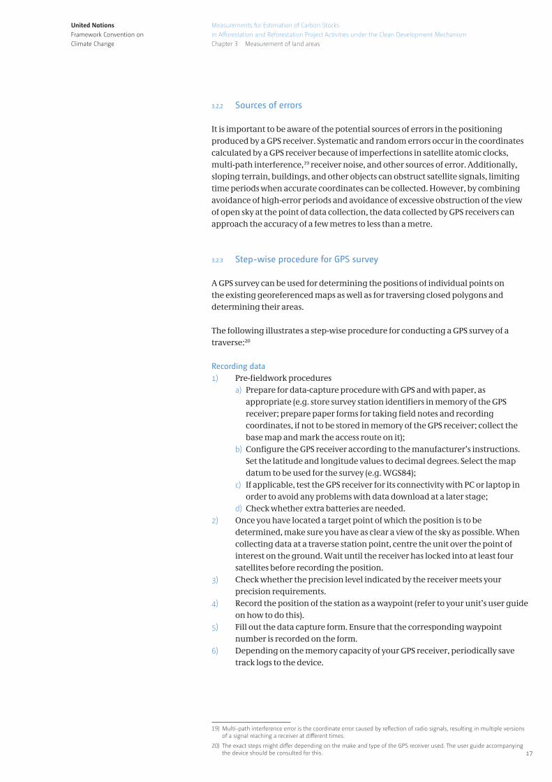
3.2.2 Sources of errors
It is important to be aware of the potential sources of errors in the positioning produced by a GPS receiver. Systematic and random errors occur in the coordinates calculated by a GPS receiver because of imperfections in satellite atomic clocks, multi-path interference,19 receiver noise, and other sources of error. Additionally, sloping terrain, buildings, and other objects can obstruct satellite signals, limiting time periods when accurate coordinates can be collected. However, by combining avoidance of high-error periods and avoidance of excessive obstruction of the view of open sky at the point of data collection, the data collected by GPS receivers can approach the accuracy of a few metres to less than a metre.
3.2.3 Step-wise procedure for GPS survey
A GPS survey can be used for determining the positions of individual points on the existing georeferenced maps as well as for traversing closed polygons and determining their areas.
The following illustrates a step-wise procedure for conducting a GPS survey of a traverse:20
Recording data1) Pre-fieldwork procedures a) Prepare for data-capture procedure with GPS and with paper, as
appropriate (e.g. store survey station identifiers in memory of the GPS receiver; prepare paper forms for taking field notes and recording coordinates, if not to be stored in memory of the GPS receiver; collect the base map and mark the access route on it);
b) Configure the GPS receiver according to the manufacturer’s instructions. Set the latitude and longitude values to decimal degrees. Select the map datum to be used for the survey (e.g. WGS84);
c) If applicable, test the GPS receiver for its connectivity with PC or laptop in order to avoid any problems with data download at a later stage;
d) Check whether extra batteries are needed.2) Once you have located a target point of which the position is to be
determined, make sure you have as clear a view of the sky as possible. When collecting data at a traverse station point, centre the unit over the point of interest on the ground. Wait until the receiver has locked into at least four satellites before recording the position.
3) Check whether the precision level indicated by the receiver meets your precision requirements.
4) Record the position of the station as a waypoint (refer to your unit’s user guide on how to do this).
5) Fill out the data capture form. Ensure that the corresponding waypoint number is recorded on the form.
6) Depending on the memory capacity of your GPS receiver, periodically save track logs to the device.
19) Multi-path interference error is the coordinate error caused by reflection of radio signals, resulting in multiple versions of a signal reaching a receiver at different times.
20) The exact steps might differ depending on the make and type of the GPS receiver used. The user guide accompanying the device should be consulted for this.

United NationsFramework Convention on Climate Change
18
Measurements for Estimation of Carbon Stocks
in Afforestation and Reforestation Project Activities under the Clean Development Mechanism
Chapter 3 Measurement of land areas
Producing map and calculating areaDepending on the capability of the receiver, data can be captured manually or stored in the receiver memory. The receiver may also be capable of processing the stored data, producing the map and estimating the distances and areas along with related uncertainties.
The data may also be transferred to a computer-based GIS application so that any further use of the data is seamlessly facilitated. This can be a significant convenience in the case where, for example, only some of the parcels or strata need to be surveyed with a GPS receiver while the rest of the parcels or strata are already delineated on documented maps.
In the simplest case, the GPS device will be capable of providing the latitudes and longitudes of the points of the surveyed traverse. These points can then be translated into local X-Y coordinates (i.e. northings and eastings) and the work of map preparation and area estimation can be carried out manually (see Appendix A for an illustrative example).
United NationsFramework Convention on Climate Change
19
Measurements for Estimation of Carbon Stocks
in Afforestation and Reforestation Project Activities under the Clean Development Mechanism
CHAPTER 4 SAMPLING PLAN
Summary The clean development mechanism methodological standards for afforestation and reforestation project activities require inventorying of forest carbon stocks by using sampling-based methods. The sampling design employed affects the cost-efficiency and precision of the estimations made thereunder. This chapter describes the sampling designs allowed under the A/R CDM methodological standards and explains how these sampling designs can be applied in practice.
4 .1 SAMPLING DESIGN
Estimation of carbon stocks in the carbon pools requires conducting forest carbon inventory based on sampling. A sampling design defines the number and spatial distribution of sample elements drawn from the sample frame. The sample frame consists of the set of all elements of interest – often all the elements constituting the population to which the estimation relates. For the purpose of carbon stock inventory based on fixed area sample plots, the population and the sampling frame are identical to the set of all possible plots of a fixed area that would cover wall-to-wall the entire area being inventoried.21 For an inventory that is based on variable area plot sampling (point sampling), the population consists of all the possible points falling in the inventoried area and hence is infinite. In this case, a sampling frame is constructed by dividing the area into a grid of square cells, the corner points (or the centre points) of which constitute the sampling frame.
The method of selection of sampling units from the sampling frame should meet the twin requirements of randomness (that is, each element of the sampling frame must have equal probability of being selected in the sample), and coverage (that is, the sample should be spread over the entire sampling frame). A commonly used sampling design in forest inventory that aims to meet these requirements in a cost-effective manner is stratified systematic sampling with a random start using fixed area sample plots.
4 .2 SAMPLING PLAN
The sampling plan of a forest carbon inventory requires decisions on the different elements of implementation of the selected sampling design.
The following aspects are considered to finalize a sampling plan:
a) Stratification; b) Shape of sample plots; c) Size of sample plots; d) Sample size and its allocation; e) Sample selection.
4.2.1 Stratification
Although stratification is not a mandatory requirement under the A/R CDM methodological standards, stratification is often desirable for cost-efficiency
21) Forest inventories commonly employ two distinct approaches to sampling: fixed area plot sampling and variable area plot sampling. Fixed area plots are also referred to as detached plots. The terms ‘plot sampling’ and ‘point sampling’ are sometimes used to contrast the two areal sampling approaches. The non-areal approach of treating individual trees as sampling units is rarely used in forest inventory.
United NationsFramework Convention on Climate Change
20
Measurements for Estimation of Carbon Stocks
in Afforestation and Reforestation Project Activities under the Clean Development Mechanism
Chapter 4 Sampling plan
considerations. The distribution of forest biomass within the project boundary is rarely, if ever, homogeneous. For efficient allocation of sample plots, the area to be inventoried is delineated into strata on the basis of the spatial pattern of distribution of carbon stocks. The ‘spatial pattern’ of distribution of carbon stocks is characterized by the following two variables:
a) The mean biomass density22 or biomass per hectare, usually expressed in tonne dry matter per hectare, as observed in sample plots; and
b) The variability of the biomass per hectare values across the sample plots.
The variability of biomass per hectare values across the inventory area can result from edaphoclimatic factors (climate and soil, aspect, slope), biological factors (species composition, age), management factors (stocking density, operations of thinning, harvest, and pruning) and disturbances (fires, pests). It is important to recognize that these factors themselves are not necessarily the preferred basis of stratification, although any of these can be the dominant determinant of biomass variability and therefore the basis of stratification.23 A single-species even-age stand is likely to qualify as a single stratum, not because of the species but because of the similar biomass per hectare values resulting from this fact. Even so, stands of different species with similar biomass per hectare values could belong to a single stratum (unless, of course, we are interested in species-wise biomass estimation for reasons other than estimation of carbon stocks).24
The area of each stratum is estimated from the delineation of the stratum boundary on the map of the inventoried area.25 The preliminary estimated mean and variance of biomass per hectare values in a stratum is used as the basis of estimation of the number of sample plots to be installed in that stratum.26
The practical application of fixed area plot sampling using systematic sample selection with a random start is illustrated through a worked example in Appendix A.
Double samplingSometimes one or more strata in the inventory area can exhibit variability of the target variable (i.e. biomass per hectare) in such a random manner that no homogeneous areas are evident (e.g. in the case where patchy growth of forest results in a clumpy structure composed of tree stands interspersed with numerous small blanks). In such a situation, delineation of strata boundaries is either not feasible or would result in defining too many strata.27 With limited possibility of gains from stratification, the sample size will have to be large in such cases. An alternative strategy to reduce the sampling cost in such cases could be to use the double sampling design.28
In double sampling, an auxiliary variable that is linearly correlated with the target variable is observed in a large first-phase sample. The auxiliary variable is so
22) In this manual we will use the terms carbon stocks and biomass almost synonymously since the two are related by a fixed constant of proportionality, viz. the carbon fraction of biomass (taken to be 0.47 for the aboveground biomass carbon pool). The sampling uncertainty of estimated carbon stocks will therefore be the same as the sampling uncertainty of estimated biomass. It is biomass that forms the direct object of estimation (target variable) in forest carbon inventories. If multiple carbon pools are being estimated in the same inventory based common sample plots, the dominant pool should form the basis of stratification (e.g. the aboveground biomass carbon pool).
23) For example, areas affected by a forest fire or areas with low growth due to poor soils can be defined as one stratum.
24) Under the A/R CDM methodological standards, the carbon fraction of biomass is taken to be the same for all species.
25) Note that field surveying may be required for delineation and determination of areas of the strata. The approaches of double sampling for stratification and sampling by post-stratification do not require delineation of strata boundaries. However, these methods are not included under the A/R CDM methodological standards.
26) The A/R CDM methodological tool Calculation of the number of sample plots for measurements within A/R CDM project activities provides the method of calculation of the number of sample plots, although any other statistical tools or package can be used for this purpose.
27) A diminishing return sets in when the project area is divided into too many strata. A small stratum will get fewer sample plots allocated and the within-stratum variance will become larger.
28) In forest inventory literature this design is also called two-phase sampling. This term should not be confused with two-stage sampling which is another name for two-stage cluster sampling.
United NationsFramework Convention on Climate Change
21
Measurements for Estimation of Carbon Stocks
in Afforestation and Reforestation Project Activities under the Clean Development Mechanism
Chapter 4 Sampling plan
selected that the cost of measurement of this variable is only a fraction of the cost of measurement of the target variable.29 In the second phase of sampling, a sub-sample is drawn from the first-phase sample and the target variable is measured in each sampling unit contained in the sub-sample. The mean and the variance of the target variable estimated from the second-phase sample are then updated by applying a regression-based adjustment which makes use of the information contained in the more extensive first-phase sample.30
The practical application of double sampling is illustrated by an example in Appendix A.
4.2.2 Shape of sample plots
Fixed area sample plots can be circular, square, rectangular, or any other shape, including a composite shape made from a number of simple geometric shapes. The plot shape should be selected in view of the specific circumstances of the forest area being inventoried.
Circular plotsCircular plots are easy to establish as only one linear measurement, the plot radius, is required. A circular plot has the lowest perimeter-to-area ratio and thus is least vulnerable to errors due to incorrect omission or inclusion of trees close to the plot boundary. In dense stands with low visibility, however, more time is required for identifying trees hidden behind other trees.
Square or rectangular plotsIn square or rectangular plots it is easier to identify and tally trees in the plot once the plot boundary has been established on the ground. These plots can be efficient in strata with high stocking density. However, square and rectangular plots are relatively difficult to establish on the ground.
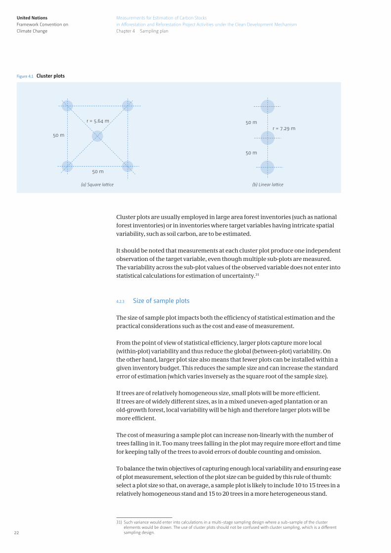
Cluster plots A cluster plot, sometimes called a combined or composite plot, consists of a number of smaller circular or rectangular plots spread out to form a geometrical figure such as a triangle or a rectangle. The objective of the composite shape is to better capture the local variability without increasing the total area sampled. However, more time is required for demarcation of the boundaries of multiple sub-plots and determination of trees located close to sub-plot boundaries as in or out.
Figure 4.1 below shows two examples of cluster plot configuration. Either of these cluster plots can be used in place of a compact circular or square plot of 500 sqm. In the configuration shown in Figure 4.1(a), five smaller circular plots, each of 100 sqm, are laid out in a square lattice spread over a linear extent of 50 m in either direction. In the configuration shown in Figure 4.1(b), three circular plots, each of 167 sqm, are laid out in linear lattice spread over a linear extent of 100 m. Of course, any other geometrical shape could have been used for the lattice. The scale over which the major part of the spatial variability of the target variable occurs should be taken into consideration while determining the extent of areal spread of the lattice. For example, the distance between sub-plots would be different for observations of littler biomass per hectare and tree biomass per hectare, as littler biomass per hectare usually shows variability over much shorter distances than tree biomass per hectare.
29) For example, measurement of basal area in a plot costs only a fraction of the cost of measuring plot biomass. Basal area has a strong correlation with plot biomass. Some vegetation indices constructed from remotely sensed data can have a significant correlation with biomass. The plot values of these indices can be easily constructed in a very large sample, or even over the entire sampling frame of a stratum.
30) As a result of the adjustment, the mean may be revised either upwards or downwards but the variance will always be lower than the variance estimated from the smaller sample. For estimation of the adjusted variance see AR-TOOL-14, equation (19).
United NationsFramework Convention on Climate Change
22
Measurements for Estimation of Carbon Stocks
in Afforestation and Reforestation Project Activities under the Clean Development Mechanism
Chapter 4 Sampling plan
(a) Square lattice (b) Linear lattice
50 m
50 m
r = 5.64 m
50 m
50 mr = 7.29 m
Figure 4.1 Cluster plots
Cluster plots are usually employed in large area forest inventories (such as national forest inventories) or in inventories where target variables having intricate spatial variability, such as soil carbon, are to be estimated.
It should be noted that measurements at each cluster plot produce one independent observation of the target variable, even though multiple sub-plots are measured. The variability across the sub-plot values of the observed variable does not enter into statistical calculations for estimation of uncertainty.31
4.2.3 Size of sample plots
The size of sample plot impacts both the efficiency of statistical estimation and the practical considerations such as the cost and ease of measurement.
From the point of view of statistical efficiency, larger plots capture more local (within-plot) variability and thus reduce the global (between-plot) variability. On the other hand, larger plot size also means that fewer plots can be installed within a given inventory budget. This reduces the sample size and can increase the standard error of estimation (which varies inversely as the square root of the sample size).
If trees are of relatively homogeneous size, small plots will be more efficient. If trees are of widely different sizes, as in a mixed uneven-aged plantation or an old-growth forest, local variability will be high and therefore larger plots will be more efficient.
The cost of measuring a sample plot can increase non-linearly with the number of trees falling in it. Too many trees falling in the plot may require more effort and time for keeping tally of the trees to avoid errors of double counting and omission.
To balance the twin objectives of capturing enough local variability and ensuring ease of plot measurement, selection of the plot size can be guided by this rule of thumb: select a plot size so that, on average, a sample plot is likely to include 10 to 15 trees in a relatively homogeneous stand and 15 to 20 trees in a more heterogeneous stand.
31) Such variance would enter into calculations in a multi-stage sampling design where a sub-sample of the cluster elements would be drawn. The use of cluster plots should not be confused with cluster sampling, which is a different sampling design.
United NationsFramework Convention on Climate Change
23
Measurements for Estimation of Carbon Stocks
in Afforestation and Reforestation Project Activities under the Clean Development Mechanism
Chapter 4 Sampling plan
Typical plot sizes used in forest inventory are 200 sqm, 400 sqm, and 500 sqm, but any size could possibly be used. Cluster plot designs can be used under appropriate conditions for reducing the plot size.
When a more precise determination of the optimum plot size is desired (e.g. in a very important stratum), a pilot study can be conducted as follows:
a) Randomly select 15 to 20 sample point locations that cover the stratum uniformly;
b) Establish and measure at each of these point locations concentric sample plots of three different sizes (small, medium and large);
c) Record the time spent in measuring each plot size;d) Calculate the variances of the mean values of the target variable measured in
the three sample plot sizes;e) The plot size that leads to the least variance per unit time is the optimum plot size.
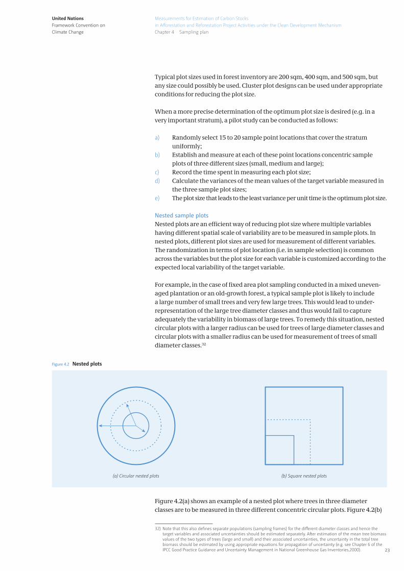
Nested sample plotsNested plots are an efficient way of reducing plot size where multiple variables having different spatial scale of variability are to be measured in sample plots. In nested plots, different plot sizes are used for measurement of different variables. The randomization in terms of plot location (i.e. in sample selection) is common across the variables but the plot size for each variable is customized according to the expected local variability of the target variable.
For example, in the case of fixed area plot sampling conducted in a mixed uneven-aged plantation or an old-growth forest, a typical sample plot is likely to include a large number of small trees and very few large trees. This would lead to under-representation of the large tree diameter classes and thus would fail to capture adequately the variability in biomass of large trees. To remedy this situation, nested circular plots with a larger radius can be used for trees of large diameter classes and circular plots with a smaller radius can be used for measurement of trees of small diameter classes.32
Figure 4.2(a) shows an example of a nested plot where trees in three diameter classes are to be measured in three different concentric circular plots. Figure 4.2(b)
32) Note that this also defines separate populations (sampling frames) for the different diameter classes and hence the target variables and associated uncertainties should be estimated separately. After estimation of the mean tree biomass values of the two types of trees (large and small) and their associated uncertainties, the uncertainty in the total tree biomass should be estimated by using appropriate equations for propagation of uncertainty (e.g. see Chapter 6 of the IPCC Good Practice Guidance and Uncertainty Management in National Greenhouse Gas Inventories,2000).
(a) Circular nested plots (b) Square nested plots
Figure 4.2 Nested plots
United NationsFramework Convention on Climate Change
24
Measurements for Estimation of Carbon Stocks
in Afforestation and Reforestation Project Activities under the Clean Development Mechanism
Chapter 4 Sampling plan
illustrates the same design for nested square plots. These nested plot designs can also be used for simultaneous inventory of different carbon pools or different components of a carbon pool (e.g. the larger plots could be used for measurement of tree biomass, the mid-sized plots could be used for measurement of shrub biomass and the small plots could be used for measurement of litter biomass).
Compared with fixed area plots, nested plots require more time to measure. The establishment of the inner plot boundaries will require time. Trees with diameters close to a diameter class threshold value will require careful examination in order to decide whether or not to measure these in a particular plot size. Any error or confusion in counting a tree as in or out of a diameter class, or in or out of a plot boundary (which might not exist as visibly marked), can lead to errors.
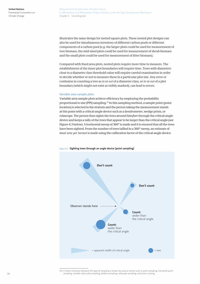
Variable area sample plotsVariable area sample plots achieve efficiency by employing the probability proportional to size (PPS) sampling.33 In this sampling method, a sample point (point location) is selected in the stratum and the person taking the measurement stands at this point with a critical-angle device such as a dendrometer, wedge prism, or relascope. The person then sights the trees around him/her through the critical-angle device and keeps a tally of the trees that appear to be larger than the critical angle (see Figure 4.3 below). A horizontal sweep of 360° is made and it is ensured that all the trees have been sighted. From the number of trees tallied in a 360° sweep, an estimate of basal area per hectare is made using the calibration factor of the critical-angle device.
33) In forest inventory literature this type of sampling is known by various names such as point sampling, horizontal point sampling, variable radius plot sampling, plotless sampling, relascope sampling, and prism cruising.
= apparent width of critical angle = tree
Figure 4.3 Sighting trees through an angle device (point sampling)
Don’t count
Don’t count
Count:wider thanthe critical angle
Count:wider thanthe critical angle
Observer stands here
United NationsFramework Convention on Climate Change
25
Measurements for Estimation of Carbon Stocks
in Afforestation and Reforestation Project Activities under the Clean Development Mechanism
Chapter 4 Sampling plan
This calibration factor is commonly called the basal area factor (BAF) of the critical-angle device. The appropriate BAF is selected keeping in view the stand density (i.e. tree stems per hectare) and the distribution of tree diameter classes. For a stratum, the BAF should be so selected that on average 5 to 12 trees would get tallied at a sample point. Commonly used BAF values are 4 m2/ha in high density stands and 1 m2/ha in low density stands with good visibility. In dense tropical rain forest, however, BAF values of up to 9 m2/ha may be appropriate.34
4.2.4 Sample size and its allocation
Once the strata boundaries have been determined and the shape and size of sample plots have been decided, the sample size (i.e. the total number of sample plots) and the allocation of the sample plots among the strata should be decided. Calculation of the total number of sample plots and their allocation among strata is carried out by applying the stepwise procedure provided in the A/R methodological tool Calculation of the number of sample plots for measurements within A/R CDM project activities, although any other software or tool, including applets freely available on the internet, can be used once the preliminary values of the stratum-wise means and coefficients of variation, and the estimated values of the strata weights, are determined. An example illustrating the practical application of the procedure for this can be found in Appendix A.
4.2.5 Sample selection
Sample selection implies drawing a sample from the sampling frame. Selection of the sampling units (sample plots or sample point locations) from the sampling frame should meet the twin objectives of randomness (to enable unbiased estimation of uncertainty) and representativeness or coverage of the area (to enable a good approximation to the population mean).
A commonly used sample selection method in forest inventory is systematic sample selection with a random start. In this method, the first sampling unit is selected in a random manner, and thereafter the remaining sampling units are so selected that the stratum area is (nearly) uniformly covered by the sample.
The practical application of this method of sample selection is explained through an illustrative example in Appendix A.
34) The choice of a BAF applies to the entire inventory, or in case of stratified sampling, to an entire stratum. In principle, choosing a different BAF at each sampling location is not allowed, as doing so would implicitly define multiple populations.
United NationsFramework Convention on Climate Change
26
Measurements for Estimation of Carbon Stocks
in Afforestation and Reforestation Project Activities under the Clean Development Mechanism
CHAPTER 5 CONDUCTING MEASUREMENTS IN SAMPLE PLOTS
Summary This chapter explains the process of conducting measurements of the variables in a sample plot. Suggested procedures include the methods of navigating to sample plot locations, establishing sample plots on ground by demarcating their boundaries, identifying trees and shrubs inside the plot and conducting the necessary measurements on these trees and shrubs. The work of conducting measurements in sample plots is the core work of a forest carbon inventory and the success of the inventory critically depends on the quality of this work.
5 .1 ESTABLISHMENT OF FIXED AREA SAMPLE PLOTS 5.1.1 Locating sample plot centre
The map locations of sample plots might have been determined in terms of local coordinates or in terms of geo-coordinates (e.g. latitudes and longitudes) determined from a map or in a GIS system. To transfer these map locations onto the ground, it will be necessary to navigate to plot centre locations in the field. The combined use of topographic maps and a GPS receiver can be an efficient way of navigating to the plot centre locations in the field. It may also be useful to enlist the help of a local guide for accessing the plot centre locations more easily.
The following stepwise procedure can be followed for this:
1) Decide the sequence in which the plots are to be established and measured. If multiple field crews are conducting the inventory simultaneously, each crew should decide this sequence among the plots under its responsibility. The sequence can be later modified as more detailed information about accessibility of individual plot locations becomes available.
2) Register the plot centre locations as GPS waypoints.35
3) Use the GPS navigation function in combination with the topographic maps or local guide’s knowledge to arrive near the plot location as far as the vehicle will go.
4) Obtain the precise GPS coordinates of the point under open sky that is nearest to the estimated location of the sample plot centre (the plot centre may or may not be under open sky).
5) Calculate the precise displacement of the plot centre location from this point in terms of northing and easting.
6) Use a tape to measure these distances and arrive at the plot centre location.7) Drive a stake (e.g. galvanized iron pipe or metal tube) at the precise location of
the plot centre.8) If obstacles prevent driving a stake at the plot centre (e.g. because of the
presence of a tree, rock, river, etc.), the stake should be fixed as close as possible to the plot centre and the distance and bearing (in degrees) of the plot centre from the stake location should be measured and recorded.
35) “Plot centre” is the centre of a circular plot. In the case of a square or rectangular plot, it could be a corner (usually the south-west corner) or the point of intersection of its diagonals. In the case of a cluster plot, the centre of the composite geometric figure (the lattice) is the plot centre. In the case of a nested plot, the centre of the largest plot is the plot centre.
United NationsFramework Convention on Climate Change
27
Measurements for Estimation of Carbon Stocks
in Afforestation and Reforestation Project Activities under the Clean Development Mechanism
Chapter 5 Conducting measurements in sample plots
9) In the vicinity of the plot centre identify at least three prominently visible fixed reference points (e.g. rock outcrop, a feature of a large tree, or a tag fixed on a witness tree). Measure distances and bearings of the plot centre from the fixed reference points and record these.
10) The geo-coordinates of the reference points are determined with the help of a GPS receiver and are recorded. Reference photos may also be taken.
11) In the case of a temporary plot, the reference points should enable quick relocation of the plot centre for re-checking of measurements for quality control.
12) In the case of a permanent plot, due regard should be paid to the probability of the reference points being durable enough within the envisaged timeframe of future measurements.
It may be useful to take photographs of the plot location site as well as of key features along the route during the access to the plot (such as road or path junctions, or settlements) that can help orient travel in the future to the plot location. A sketch of the access route should be drawn on the topographic map and should be attached to the field data form, with indications of the reference points that will facilitate relocation of the plot. If required, coloured flagging tape should be placed on trees along the access route. The tape should be visible enough to facilitate the return of the field team out of the plot location. In the case of a permanent plot, a photo from the plot centre should be taken for each of the reference features and recorded with an appropriate description.
5.1.2 Plot boundary demarcation
The correct and precise demarcation of the plot boundary is important to avoid errors and bias in estimation.
The following aspects should be taken into consideration while conducting plot boundary demarcation in the field:
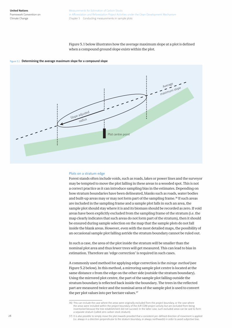
Ground slopeFixed area plot sampling is based on the assumption that sample plots are laid out in the horizontal plane. If a sample plot is located on sloping ground, a slope correction should be applied to account for the fact that distances measured along a slope become smaller when they are projected on the horizontal plane. In the case of circular plots, the slope correction can be applied by enlarging the radius of the plot by a factor of where is the slope of the ground in the direction of the average maximum slope. In the case of a square plot, the sides perpendicular to the direction of the average maximum slope should remain unaffected and the sides parallel to the direction of the average maximum slope should be enlarged by a factor of .
United NationsFramework Convention on Climate Change
28
Measurements for Estimation of Carbon Stocks
in Afforestation and Reforestation Project Activities under the Clean Development Mechanism
Chapter 5 Conducting measurements in sample plots
Figure 5.1 below illustrates how the average maximum slope at a plot is defined when a compound ground slope exists within the plot.
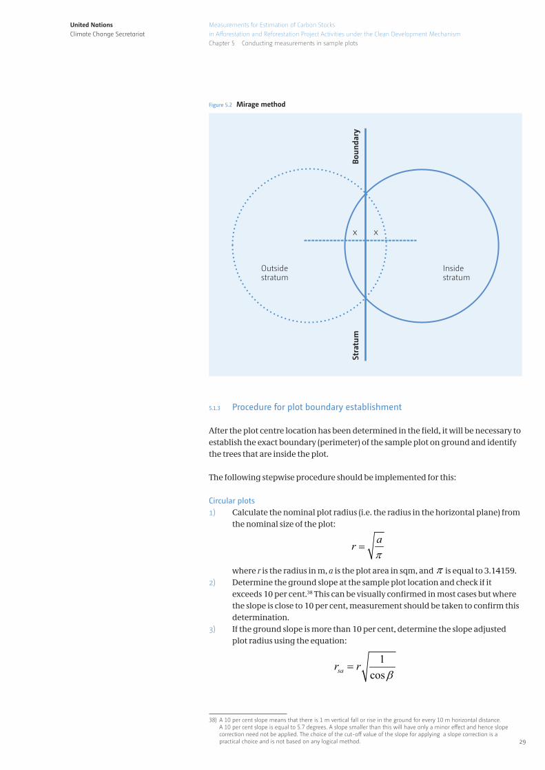
Plots on a stratum edge Forest stands often include voids, such as roads, lakes or power lines and the surveyor may be tempted to move the plot falling in these areas to a wooded spot. This is not a correct practice as it can introduce sampling bias in the estimates. Depending on how stratum boundaries have been delineated, blanks such as roads, water bodies and built-up areas may or may not form part of the sampling frame.36 If such areas are included in the sampling frame and a sample plot falls in such an area, the sample plot should stay where it is and its biomass should be recorded as zero. If void areas have been explicitly excluded from the sampling frame of the stratum (i.e. the map clearly indicates that such areas do not form part of the stratum), then it should be ensured during sample selection on the map that the sample plots do not fall inside the blank areas. However, even with the most detailed maps, the possibility of an occasional sample plot falling astride the stratum boundary cannot be ruled out.
In such a case, the area of the plot inside the stratum will be smaller than the nominal plot area and thus fewer trees will get measured. This can lead to bias in estimation. Therefore an ‘edge correction’ is required in such cases.
A commonly used method for applying edge correction is the mirage method (see Figure 5.2 below). In this method, a mirroring sample plot centre is located at the same distance x from the edge on the other side (outside the stratum boundary). Using the mirrored plot centre, the part of the sample plot falling outside the stratum boundary is reflected back inside the boundary. The trees in the reflected part are measured twice and the nominal area of the sample plot is used to convert the per plot values into per hectare values.37
Plot centre point
Slope adjusted
Average
maximum slope
radius
Figure 5.1 Determining the average maximum slope for a compound slope
36) This can include the case where the areas were originally excluded from the project boundary, or the case where the areas were included within the project boundary of the A/R CDM project activity but are excluded from being inventoried because the tree establishment did not succeed. In the latter case, such excluded areas can be said to form a separate stratum (called zero carbon stock stratum).
37) It is also possible to simply move the plot inwards provided that a consistent pre-defined direction of movement is applied (i.e. always in a direction perpendicular to the stratum boundary, or always northwards) in order to avoid subjective bias.
29
Measurements for Estimation of Carbon Stocks
in Afforestation and Reforestation Project Activities under the Clean Development Mechanism
Chapter 5 Conducting measurements in sample plots
United NationsClimate Change Secretariat
5.1.3 Procedure for plot boundary establishment
After the plot centre location has been determined in the field, it will be necessary to establish the exact boundary (perimeter) of the sample plot on ground and identify the trees that are inside the plot.
The following stepwise procedure should be implemented for this:
Circular plots1) Calculate the nominal plot radius (i.e. the radius in the horizontal plane) from the nominal size of the plot:
where r is the radius in m, a is the plot area in sqm, and π is equal to 3.14159. 2) Determine the ground slope at the sample plot location and check if it
exceeds 10 per cent.38 This can be visually confirmed in most cases but where the slope is close to 10 per cent, measurement should be taken to confirm this determination.
3) If the ground slope is more than 10 per cent, determine the slope adjusted plot radius using the equation:
38) A 10 per cent slope means that there is 1 m vertical fall or rise in the ground for every 10 m horizontal distance. A 10 per cent slope is equal to 5.7 degrees. A slope smaller than this will have only a minor effect and hence slope correction need not be applied. The choice of the cut-off value of the slope for applying a slope correction is a practical choice and is not based on any logical method.
x x
Stra
tum
Bou
ndar
y
Outsidestratum
Insidestratum
Figure 5.2 Mirage method
arπ
=
1cossar r
β=
United NationsFramework Convention on Climate Change
30
Measurements for Estimation of Carbon Stocks
in Afforestation and Reforestation Project Activities under the Clean Development Mechanism
Chapter 5 Conducting measurements in sample plots
where sar is the slope-adjusted radius, r is the nominal radius, and β is the slope of the ground in the direction of the average maximum slope rounded off to the nearest degree.
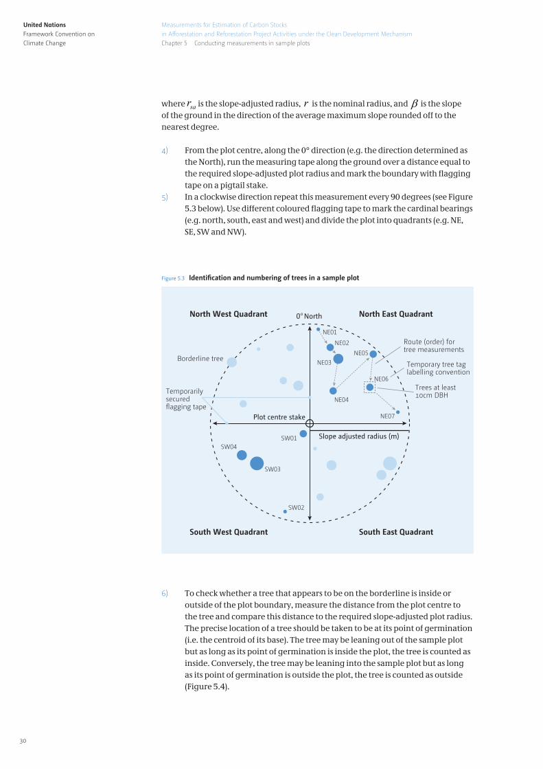
4) From the plot centre, along the 0° direction (e.g. the direction determined as the North), run the measuring tape along the ground over a distance equal to the required slope-adjusted plot radius and mark the boundary with flagging tape on a pigtail stake.
5) In a clockwise direction repeat this measurement every 90 degrees (see Figure 5.3 below). Use different coloured flagging tape to mark the cardinal bearings (e.g. north, south, east and west) and divide the plot into quadrants (e.g. NE, SE, SW and NW).
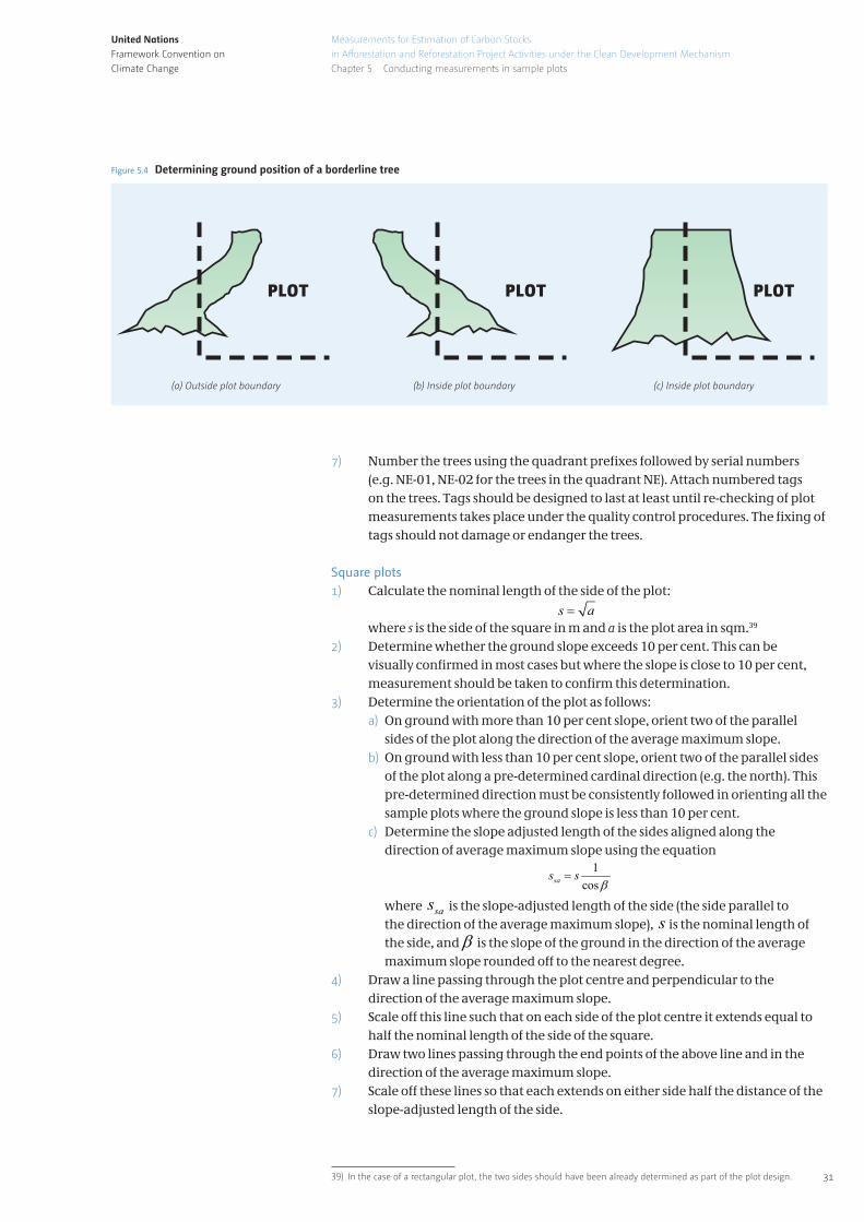
6) To check whether a tree that appears to be on the borderline is inside or outside of the plot boundary, measure the distance from the plot centre to the tree and compare this distance to the required slope-adjusted plot radius. The precise location of a tree should be taken to be at its point of germination (i.e. the centroid of its base). The tree may be leaning out of the sample plot but as long as its point of germination is inside the plot, the tree is counted as inside. Conversely, the tree may be leaning into the sample plot but as long as its point of germination is outside the plot, the tree is counted as outside (Figure 5.4).
North West Quadrant North East Quadrant
South West Quadrant South East Quadrant
Route (order) fortree measurements
Temporary tree taglabelling convention
Trees at least10cm DBHTemporarily
secured�agging tape
Borderline tree
Slope adjusted radius (m)
Plot centre stake
0 o North
SW04
SW03
SW01
NE04
NE07
NE06
NE05
NE03
NE02
NE01
SW02
Figure 5.3 Identi cation and numbering of trees in a sample plot
United NationsFramework Convention on Climate Change
31
Measurements for Estimation of Carbon Stocks
in Afforestation and Reforestation Project Activities under the Clean Development Mechanism
Chapter 5 Conducting measurements in sample plots
7) Number the trees using the quadrant prefixes followed by serial numbers (e.g. NE-01, NE-02 for the trees in the quadrant NE). Attach numbered tags on the trees. Tags should be designed to last at least until re-checking of plot measurements takes place under the quality control procedures. The fixing of tags should not damage or endanger the trees.
Square plots1) Calculate the nominal length of the side of the plot:
where s is the side of the square in m and a is the plot area in sqm.39
2) Determine whether the ground slope exceeds 10 per cent. This can be visually confirmed in most cases but where the slope is close to 10 per cent, measurement should be taken to confirm this determination.
3) Determine the orientation of the plot as follows: a) On ground with more than 10 per cent slope, orient two of the parallel
sides of the plot along the direction of the average maximum slope. b) On ground with less than 10 per cent slope, orient two of the parallel sides
of the plot along a pre-determined cardinal direction (e.g. the north). This pre-determined direction must be consistently followed in orienting all the sample plots where the ground slope is less than 10 per cent.
c) Determine the slope adjusted length of the sides aligned along the direction of average maximum slope using the equation
where sas is the slope-adjusted length of the side (the side parallel to the direction of the average maximum slope), s is the nominal length of the side, and β is the slope of the ground in the direction of the average maximum slope rounded off to the nearest degree.
4) Draw a line passing through the plot centre and perpendicular to the direction of the average maximum slope.
5) Scale off this line such that on each side of the plot centre it extends equal to half the nominal length of the side of the square.
6) Draw two lines passing through the end points of the above line and in the direction of the average maximum slope.
7) Scale off these lines so that each extends on either side half the distance of the slope-adjusted length of the side.
(a) Outside plot boundary (b) Inside plot boundary (c) Inside plot boundary
PLOT PLOT PLOT
Figure 5.4 Determining ground position of a borderline tree
39) In the case of a rectangular plot, the two sides should have been already determined as part of the plot design.
1cossas s
β=
s a=
United NationsFramework Convention on Climate Change
32
Measurements for Estimation of Carbon Stocks
in Afforestation and Reforestation Project Activities under the Clean Development Mechanism
Chapter 5 Conducting measurements in sample plots
8) Having fixed the four corners as the intersections of the extended lines, measure the diagonals of the plot and check for correctness of the plot boundary by comparing this with a computed length of the diagonals (i.e. the square root of the sum of the squares of the two mutually perpendicular sides).
9) If the computed and measured lengths of the diagonals differ by more than 5 per cent, re-check the angles and distances and re-determine the positions of the four corner points until the measured values of the diagonals are in agreement with the calculated values.
10) To check borderline trees, stretch coloured tape along each of the four sides of the square (one after another, not necessarily at the same time) and determine whether trees near the plot boundary are inside or outside of the plot.
11) Temporarily tag the trees determined to be inside the plot. Number the trees using the quadrant prefixes followed by serial numbers, e.g. NE-01, NE-02 for the trees in the quadrant NE (see Figure 5.3 above). Attach numbered tags on the trees. Tags should be designed to last at least until the re-checking of the plot measurements takes place under quality control procedures. The fixing of tags should not damage or endanger the trees.
Cluster plotsA cluster plot should be laid down following a procedure similar to the above procedure. It will require more time to precisely locate the sub-plot centres and establish the boundaries (perimeters) of the sub-plots constituting the cluster plot. The orientation of the cluster lattice should be pre-decided and should not be arbitrarily decided at the time of establishment of plots. That is, in the case of a cluster plot design shown in Figure 4.1, if two parallel sides of the lattice are aligned north-south, it should be consistently done so at all sample plot locations. Note that only the radii of the sub-plots need to be adjusted for ground slope and not the lattice distances as these distances do not enter into the calculations of the target variable and do not contribute to the bias or the variance of the estimated value of the target variable.
5 .2 MEASUREMENTS IN FIXED AREA SAMPLE PLOTS
Once the plot boundary has been established and the trees inside the plot boundary have been determined and tagged, measurements would need to be conducted on the trees and other components of carbon pools. This sub-section describes the procedures to be followed in conducting measurements in sample plots.
5.2.1 Measurement of trees
All trees that have been determined to be inside a sample plot are measured.40
Basic information about treesThe following basic information about the trees subjected to measurements should be recorded so as to facilitate any subsequent quality control work:
1) Tree species: Local name and scientific (Latin) name2) Tree status: Live standing: Leaning in/out of the plot; Live fallen: Fallen in/out of the plot3) Stem status: Forked above/below measurement level; Number of stems (stems measured separately)
40) In practice, only trees having diameter above a minimum diameter (e.g. commonly fixed as 5 cm or 10 cm) are measured. Young trees that do not meet the minimum diameter requirement are considered saplings. Biomass of saplings is either ignored or estimated by using a separate method (see AR-TOOL14, appendix 1, paragraph 3).
United NationsFramework Convention on Climate Change
33
Measurements for Estimation of Carbon Stocks
in Afforestation and Reforestation Project Activities under the Clean Development Mechanism
Chapter 5 Conducting measurements in sample plots
One or more of the dimensions of the trees determined to be inside the plot are measured, depending on the model being used for conversion of tree dimensions into tree biomass.
Tree diameter Tree diameter can be defined in different ways. It is important that the tree diameter is measured in a manner that is consistent with the model being used for conversion of tree diameter into tree biomass. For example, if the model (e.g. an allometric equation) requires root collar diameter (drc) as an input variable, measuring the diameter at breast height (dbh) will not be useful (and vice versa).
Diameter at breast height or dbh is the most commonly used tree diameter in forest inventories. It is usually defined as the over-bark tree stem diameter measured at a pre-determined height above the ground level. The pre-determined height, called the breast height, is variously fixed as 1.30 m, 1.37 m or 1.40 m in different national forest inventories. The breast height adopted for a forest carbon inventory should correspond to the definition of dbh that was used for developing the model (i.e. the volume equations or allometric equations) to be used in the inventory. If it is not known at what height the dbh was measured for developing the model being used, the dbh should be measured at a height of 1.40 m.41
The following stepwise procedure is implemented for measurement of the dbh of a tree in a sample plot:
1) Determine the highest point of mineral soil or humus layer on the uphill side at the base of the tree.
2) From this point on the ground, locate the point at a distance equal to the breast height (e.g. 1.40 m) along the stem axis.
3) Measure the stem diameter at this point to the nearest 0.1 cm using a diameter tape or diameter callipers.
4) If using diameter callipers (see Figure 5.5 below), the following precautions should be kept in mind:
a) The graduated beam of the callipers must be perfectly straight and the graduations should be clearly visible.
b) The movable and the fixed arms should run exactly parallel to each other and perpendicular to the graduated beam and the three should stay in a plane perpendicular to the axis of the tree stem.
c) The point of measurement should be correctly positioned. A wooden T-bar of height equal to the selected breast height can be used for ensuring this consistently.
d) Excessive pressure should not be exerted during measurement as it can lead to operator-bias because of squeezing of the bark. Insufficient pressure can also lead to bias as bark surface irregularities can make the recorded diameter larger than it actually is.
e) The callipers should be calibrated regularly. They should be capable of measuring diameter to the precision of 0.10 cm.
f) The stem diameter should be measured in two mutually perpendicular directions and the geometric mean of the two diameters should be recorded as the measured diameter.
41) This follows from the principle of conservativeness being applied in cases of ambiguity or uncertainty.
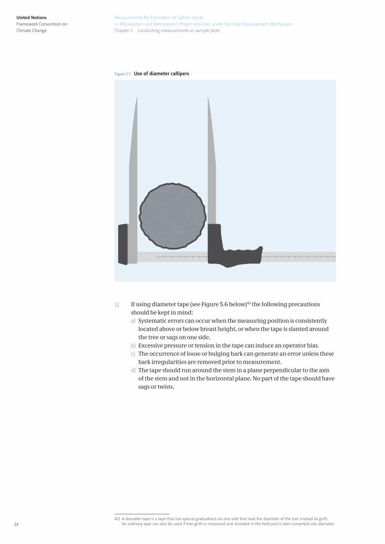
United NationsFramework Convention on Climate Change
34
Measurements for Estimation of Carbon Stocks
in Afforestation and Reforestation Project Activities under the Clean Development Mechanism
Chapter 5 Conducting measurements in sample plots
5) If using diameter tape (see Figure 5.6 below)42 the following precautions should be kept in mind:
a) Systematic errors can occur when the measuring position is consistently located above or below breast height, or when the tape is slanted around the tree or sags on one side.
b) Excessive pressure or tension in the tape can induce an operator bias. c) The occurrence of loose or bulging bark can generate an error unless these
bark irregularities are removed prior to measurement. d) The tape should run around the stem in a plane perpendicular to the axis
of the stem and not in the horizontal plane. No part of the tape should have sags or twists.
Figure 5.5 Use of diameter callipers
42) A diameter tape is a tape that has special graduations on one side that read the diameter of the tree instead its girth. An ordinary tape can also be used if tree girth is measured and recorded in the field and is later converted into diameter.
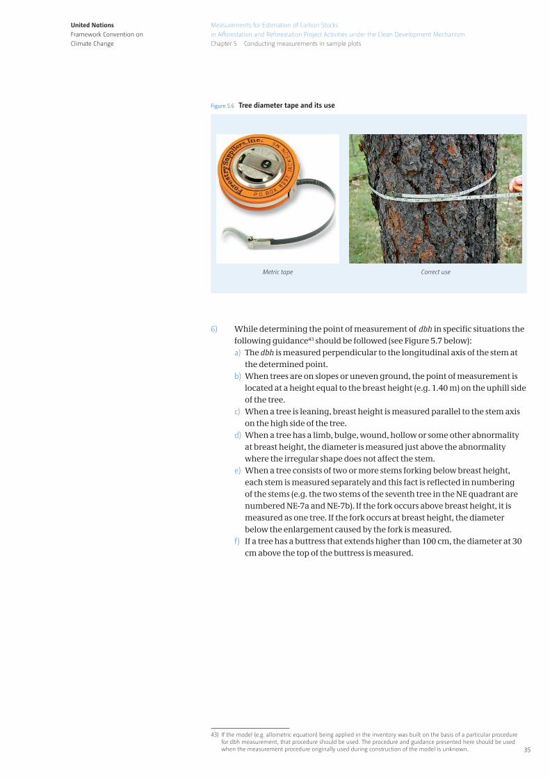
United NationsFramework Convention on Climate Change
35
Measurements for Estimation of Carbon Stocks
in Afforestation and Reforestation Project Activities under the Clean Development Mechanism
Chapter 5 Conducting measurements in sample plots
6) While determining the point of measurement of dbh in specific situations the following guidance43 should be followed (see Figure 5.7 below):
a) The dbh is measured perpendicular to the longitudinal axis of the stem at the determined point.
b) When trees are on slopes or uneven ground, the point of measurement is located at a height equal to the breast height (e.g. 1.40 m) on the uphill side of the tree.
c) When a tree is leaning, breast height is measured parallel to the stem axis on the high side of the tree.
d) When a tree has a limb, bulge, wound, hollow or some other abnormality at breast height, the diameter is measured just above the abnormality where the irregular shape does not affect the stem.
e) When a tree consists of two or more stems forking below breast height, each stem is measured separately and this fact is reflected in numbering of the stems (e.g. the two stems of the seventh tree in the NE quadrant are numbered NE-7a and NE-7b). If the fork occurs above breast height, it is measured as one tree. If the fork occurs at breast height, the diameter below the enlargement caused by the fork is measured.
f) If a tree has a buttress that extends higher than 100 cm, the diameter at 30 cm above the top of the buttress is measured.
Correct useMetric tape
Figure 5.6 Tree diameter tape and its use
43) If the model (e.g. allometric equation) being applied in the inventory was built on the basis of a particular procedure for dbh measurement, that procedure should be used. The procedure and guidance presented here should be used when the measurement procedure originally used during construction of the model is unknown.
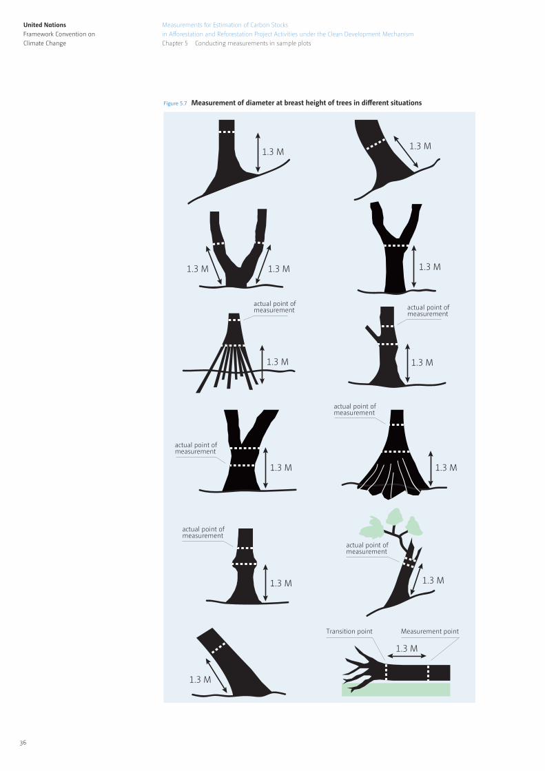
United NationsFramework Convention on Climate Change
36
Measurements for Estimation of Carbon Stocks
in Afforestation and Reforestation Project Activities under the Clean Development Mechanism
Chapter 5 Conducting measurements in sample plots
1.3 M
1.3 M
1.3 M
1.3 M
1.3 M1.3 M
Transition point Measurement point
1.3 M
actual point ofmeasurement
1.3 M1.3 M
actual point ofmeasurement
1.3 M
actual point ofmeasurement
1.3 M
actual point ofmeasurement
1.3 M
actual point ofmeasurement
1.3 M
actual point ofmeasurement
Figure 5.7 Measurement of diameter at breast height of trees in different situations
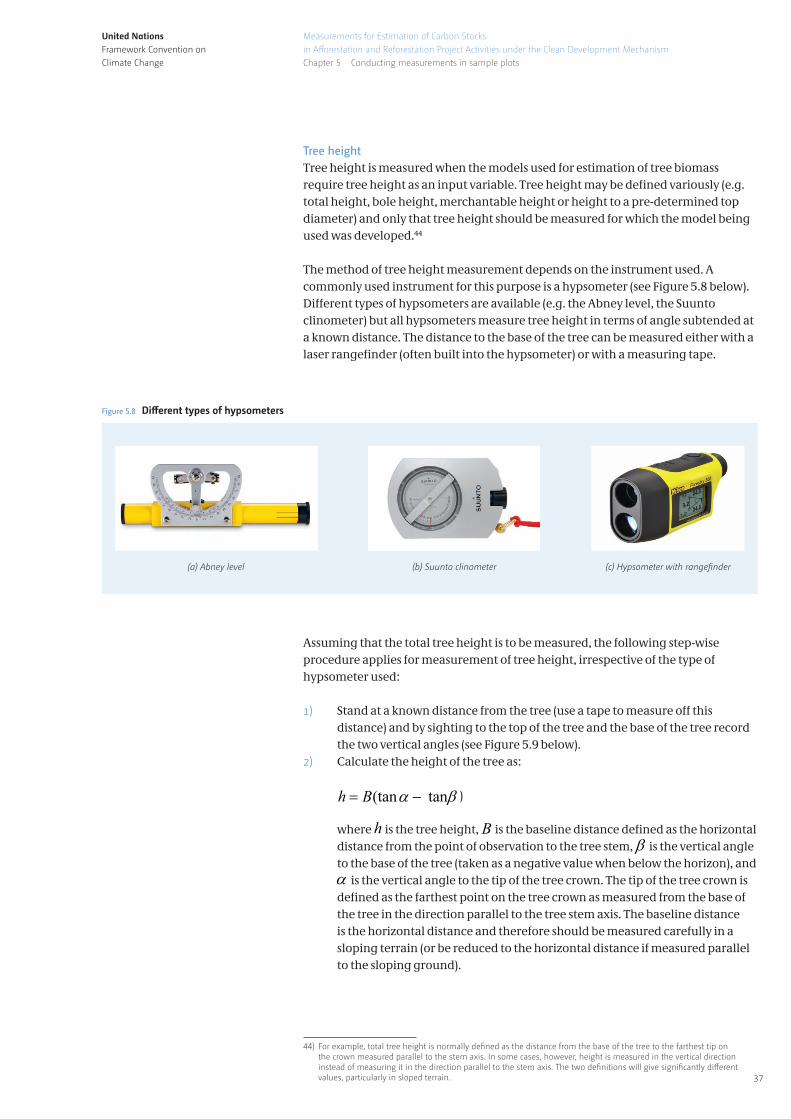
United NationsFramework Convention on Climate Change
37
Measurements for Estimation of Carbon Stocks
in Afforestation and Reforestation Project Activities under the Clean Development Mechanism
Chapter 5 Conducting measurements in sample plots
Tree height Tree height is measured when the models used for estimation of tree biomass require tree height as an input variable. Tree height may be defined variously (e.g. total height, bole height, merchantable height or height to a pre-determined top diameter) and only that tree height should be measured for which the model being used was developed.44
The method of tree height measurement depends on the instrument used. A commonly used instrument for this purpose is a hypsometer (see Figure 5.8 below). Different types of hypsometers are available (e.g. the Abney level, the Suunto clinometer) but all hypsometers measure tree height in terms of angle subtended at a known distance. The distance to the base of the tree can be measured either with a laser rangefinder (often built into the hypsometer) or with a measuring tape.
Assuming that the total tree height is to be measured, the following step-wise procedure applies for measurement of tree height, irrespective of the type of hypsometer used:
1) Stand at a known distance from the tree (use a tape to measure off this distance) and by sighting to the top of the tree and the base of the tree record the two vertical angles (see Figure 5.9 below).
2) Calculate the height of the tree as:
)
where h is the tree height, B is the baseline distance defined as the horizontal distance from the point of observation to the tree stem, β is the vertical angle to the base of the tree (taken as a negative value when below the horizon), and α is the vertical angle to the tip of the tree crown. The tip of the tree crown is defined as the farthest point on the tree crown as measured from the base of the tree in the direction parallel to the tree stem axis. The baseline distance is the horizontal distance and therefore should be measured carefully in a sloping terrain (or be reduced to the horizontal distance if measured parallel to the sloping ground).
44) For example, total tree height is normally defined as the distance from the base of the tree to the farthest tip on the crown measured parallel to the stem axis. In some cases, however, height is measured in the vertical direction instead of measuring it in the direction parallel to the stem axis. The two definitions will give significantly different values, particularly in sloped terrain.
(a) Abney level (b) Suunto clinometer (c) Hypsometer with range�nder
Figure 5.8 Different types of hypsometers
(tan tanh B α β= −
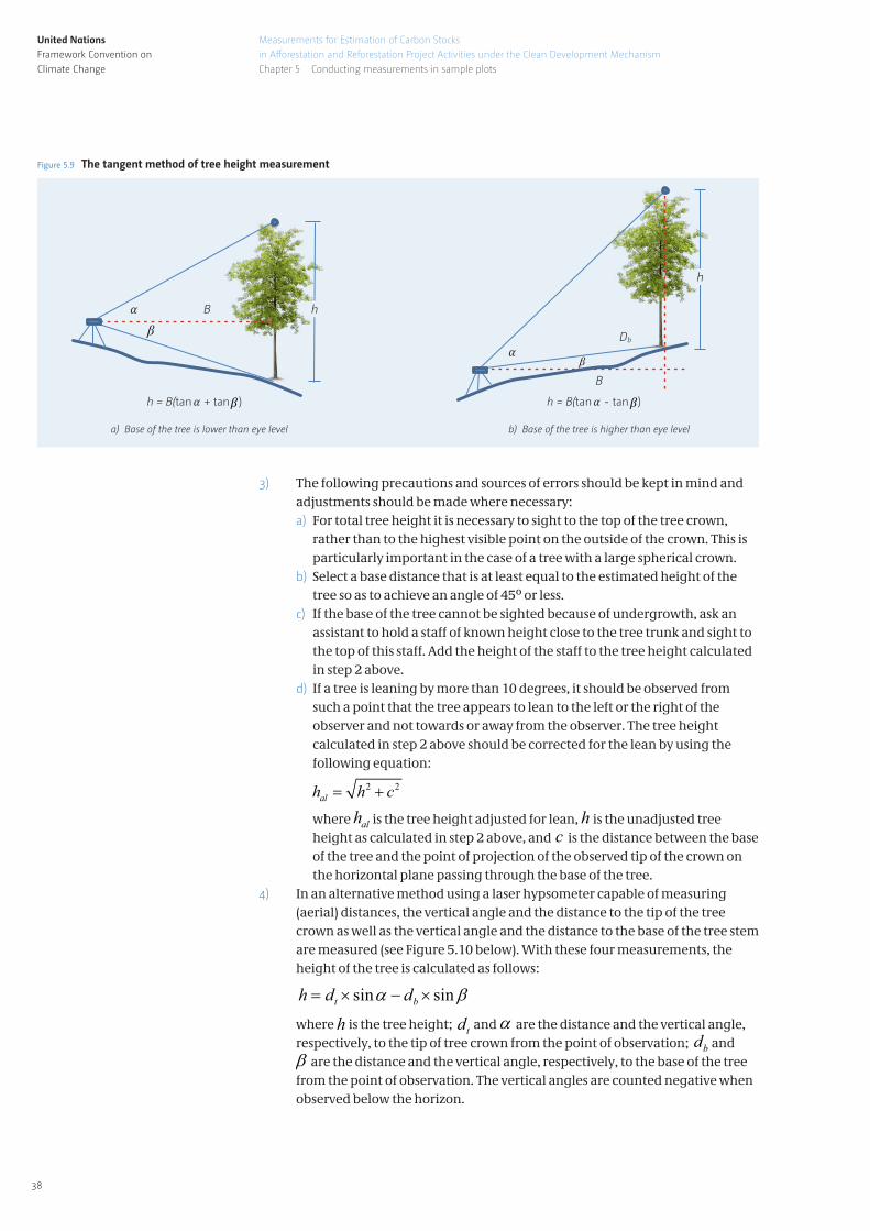
United NationsFramework Convention on Climate Change
38
Measurements for Estimation of Carbon Stocks
in Afforestation and Reforestation Project Activities under the Clean Development Mechanism
Chapter 5 Conducting measurements in sample plots
3) The following precautions and sources of errors should be kept in mind and adjustments should be made where necessary:
a) For total tree height it is necessary to sight to the top of the tree crown, rather than to the highest visible point on the outside of the crown. This is particularly important in the case of a tree with a large spherical crown.
b) Select a base distance that is at least equal to the estimated height of the tree so as to achieve an angle of 45º or less.
c) If the base of the tree cannot be sighted because of undergrowth, ask an assistant to hold a staff of known height close to the tree trunk and sight to the top of this staff. Add the height of the staff to the tree height calculated in step 2 above.
d) If a tree is leaning by more than 10 degrees, it should be observed from such a point that the tree appears to lean to the left or the right of the observer and not towards or away from the observer. The tree height calculated in step 2 above should be corrected for the lean by using the following equation:
where alh is the tree height adjusted for lean, h is the unadjusted tree height as calculated in step 2 above, and c is the distance between the base of the tree and the point of projection of the observed tip of the crown on the horizontal plane passing through the base of the tree.
4) In an alternative method using a laser hypsometer capable of measuring (aerial) distances, the vertical angle and the distance to the tip of the tree crown as well as the vertical angle and the distance to the base of the tree stem are measured (see Figure 5.10 below). With these four measurements, the height of the tree is calculated as follows:
where h is the tree height; td andα are the distance and the vertical angle, respectively, to the tip of tree crown from the point of observation; bd and β are the distance and the vertical angle, respectively, to the base of the tree from the point of observation. The vertical angles are counted negative when observed below the horizon.
a) Base of the tree is lower than eye level b) Base of the tree is higher than eye level
B
βh
h = B(tan + tan )𝛼𝛼 𝛽𝛽
B
Db
β
h
h = B(tan - tan )𝛼𝛼 𝛽𝛽
𝛼𝛼
𝛼𝛼
Figure 5.9 The tangent method of tree height measurement
2 2alh h c= +
sin sint bh d dα β= × − ×
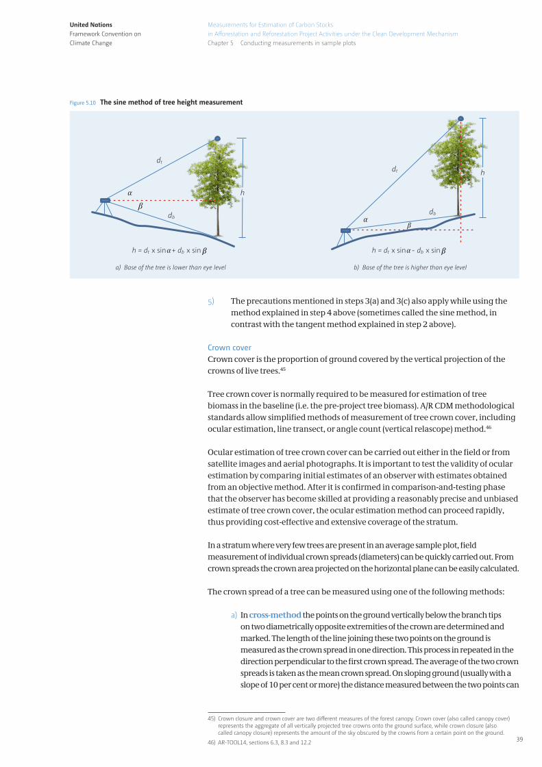
United NationsFramework Convention on Climate Change
39
Measurements for Estimation of Carbon Stocks
in Afforestation and Reforestation Project Activities under the Clean Development Mechanism
Chapter 5 Conducting measurements in sample plots
5) The precautions mentioned in steps 3(a) and 3(c) also apply while using the method explained in step 4 above (sometimes called the sine method, in contrast with the tangent method explained in step 2 above).
Crown coverCrown cover is the proportion of ground covered by the vertical projection of the crowns of live trees.45
Tree crown cover is normally required to be measured for estimation of tree biomass in the baseline (i.e. the pre-project tree biomass). A/R CDM methodological standards allow simplified methods of measurement of tree crown cover, including ocular estimation, line transect, or angle count (vertical relascope) method.46
Ocular estimation of tree crown cover can be carried out either in the field or from satellite images and aerial photographs. It is important to test the validity of ocular estimation by comparing initial estimates of an observer with estimates obtained from an objective method. After it is confirmed in comparison-and-testing phase that the observer has become skilled at providing a reasonably precise and unbiased estimate of tree crown cover, the ocular estimation method can proceed rapidly, thus providing cost-effective and extensive coverage of the stratum.
In a stratum where very few trees are present in an average sample plot, field measurement of individual crown spreads (diameters) can be quickly carried out. From crown spreads the crown area projected on the horizontal plane can be easily calculated.
The crown spread of a tree can be measured using one of the following methods:
a) In cross-method the points on the ground vertically below the branch tips on two diametrically opposite extremities of the crown are determined and marked. The length of the line joining these two points on the ground is measured as the crown spread in one direction. This process in repeated in the direction perpendicular to the first crown spread. The average of the two crown spreads is taken as the mean crown spread. On sloping ground (usually with a slope of 10 per cent or more) the distance measured between the two points can
45) Crown closure and crown cover are two different measures of the forest canopy. Crown cover (also called canopy cover) represents the aggregate of all vertically projected tree crowns onto the ground surface, while crown closure (also called canopy closure) represents the amount of the sky obscured by the crowns from a certain point on the ground.
46) AR-TOOL14, sections 6.3, 8.3 and 12.2
a) Base of the tree is lower than eye level b) Base of the tree is higher than eye level
βh
h = dt x sin + db x sin𝛼𝛼 𝛽𝛽
dbdb
dt
dt
β
h
𝛼𝛼
𝛼𝛼
h = dt x sin - db x sin𝛼𝛼 𝛽𝛽
Figure 5.10 The sine method of tree height measurement
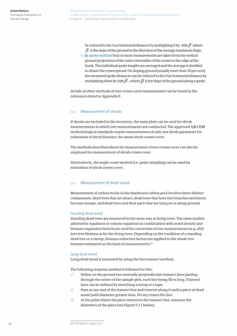
United NationsFramework Convention on Climate Change
40
Measurements for Estimation of Carbon Stocks
in Afforestation and Reforestation Project Activities under the Clean Development Mechanism
Chapter 5 Conducting measurements in sample plots
be reduced to the true horizontal distance by multiplying it by cosβ whereβ is the slope of the ground in the direction of the average maximum slope.
b) In spoke method four or more measurements are taken from the vertical ground projections of the outer extremities of the crown to the edge of the trunk. The individual spoke lengths are averaged and the average is doubled to obtain the crown spread. On sloping ground (usually more than 10 per cent) the measured spoke distances can be reduced to the true horizontal distance by multiplying these by cosβ , whereβ is the slope of the ground along a spoke.
Details of other methods of tree crown cover measurement can be found in the references listed in Appendix E.
5.2.2 Measurement of shrubs
If shrubs are included in the inventory, the same plots can be used for shrub measurements in which tree measurements are conducted. The approved A/R CDM methodological standards require measurement of only one shrub parameter for estimation of shrub biomass: the mean shrub crown cover.
The methods described above for measurement of tree crown cover can also be employed for measurement of shrub crown cover.
Alternatively, the angle count method (i.e. point sampling) can be used for estimation of shrub crown cover.
5.2.3 Measurement of dead wood
Measurement of carbon stocks in the deadwood carbon pool involves three distinct components: dead trees that are intact, dead trees that have lost branches and hence become stumps, and dead trees and their parts that are lying on or along ground.
Standing dead woodStanding dead trees are measured in the same way as living trees. The same models (allometric equations or volume equations in combination with wood density and biomass expansion factors) are used for conversion of tree measurements (e.g. dbh) into tree biomass as for the living trees. Depending on the condition of a standing dead tree or a stump, biomass reduction factors are applied to the whole tree biomass estimated on the basis of measurements.47
Lying dead woodLying dead wood is measured by using the line transect method.
The following stepwise method is followed for this:1) Define on the ground two mutually perpendicular transect lines passing
through the centre of the sample plot, each line being 50 m long. Transect lines can be defined by stretching a string or a tape.
2) Start at one end of the transect line and traverse along it until a piece of dead wood (with diameter greater than 10 cm) crosses the line.
3) At the point where the piece intersects the transect line, measure the diameters of the piece (see Figure 5.11 below).
47) AR-TOOL12, section 6.1.1
United NationsFramework Convention on Climate Change
41
Measurements for Estimation of Carbon Stocks
in Afforestation and Reforestation Project Activities under the Clean Development Mechanism
Chapter 5 Conducting measurements in sample plots
4) Determine the decay class into which the piece of wood falls, using the pre- defined decay class criteria (e.g. the machete test) and note the related density reduction factor.48
5) Input the data into the relevant equation of the A/R methodological tool Estimation of carbon stocks and change in carbon stocks in dead wood and litter in A/R CDM project activities to estimate the carbon stock in lying dead wood in the plot.
5.2.4 Measurement of litter
Litter measurements are conducted by collecting samples of litter from the same sample plots in which tree measurements are conducted. Samples of litter are collected by using a wire frame (usually 1 m square) which defines the perimeter of sub-plots for litter measurement.
The following stepwise procedure is followed for this:
1) Place the sampling frame in four randomly selected places within the sample plot so that the plot is well covered by the four locations.
2) Collect all the litter within the perimeter defined by each position of the sample frame. Mix the four litter samples into one composite sample.
3) Weigh the composite sample and record its fresh weight. 4) Take a sub-sample from the composite sample and record its fresh weight.5) Dry the sub-sample at a temperature of 70 degrees Celsius for 48 hours and
record its dry weight.6) Input the data into the relevant equation of the A/R methodological tool
Estimation of carbon stocks and change in carbon stocks in dead wood and litter in A/R CDM project activities to estimate the carbon stock in litter in the plot.
5 .3 ESTABLISHMENT OF VARIABLE AREA SAMPLE PLOTS
In variable area plot sampling, only the plot centre location needs to be established in the field, since the plot boundary is not fixed.
For establishing a plot centre location in the field, the method explained in section 5.1.2 above is followed.
Figure 5.11 Diameter is measured perpendicular to the axis of the log or branch of a log crossing the transect line
48) AR-TOOL12, section 6.1.1.4
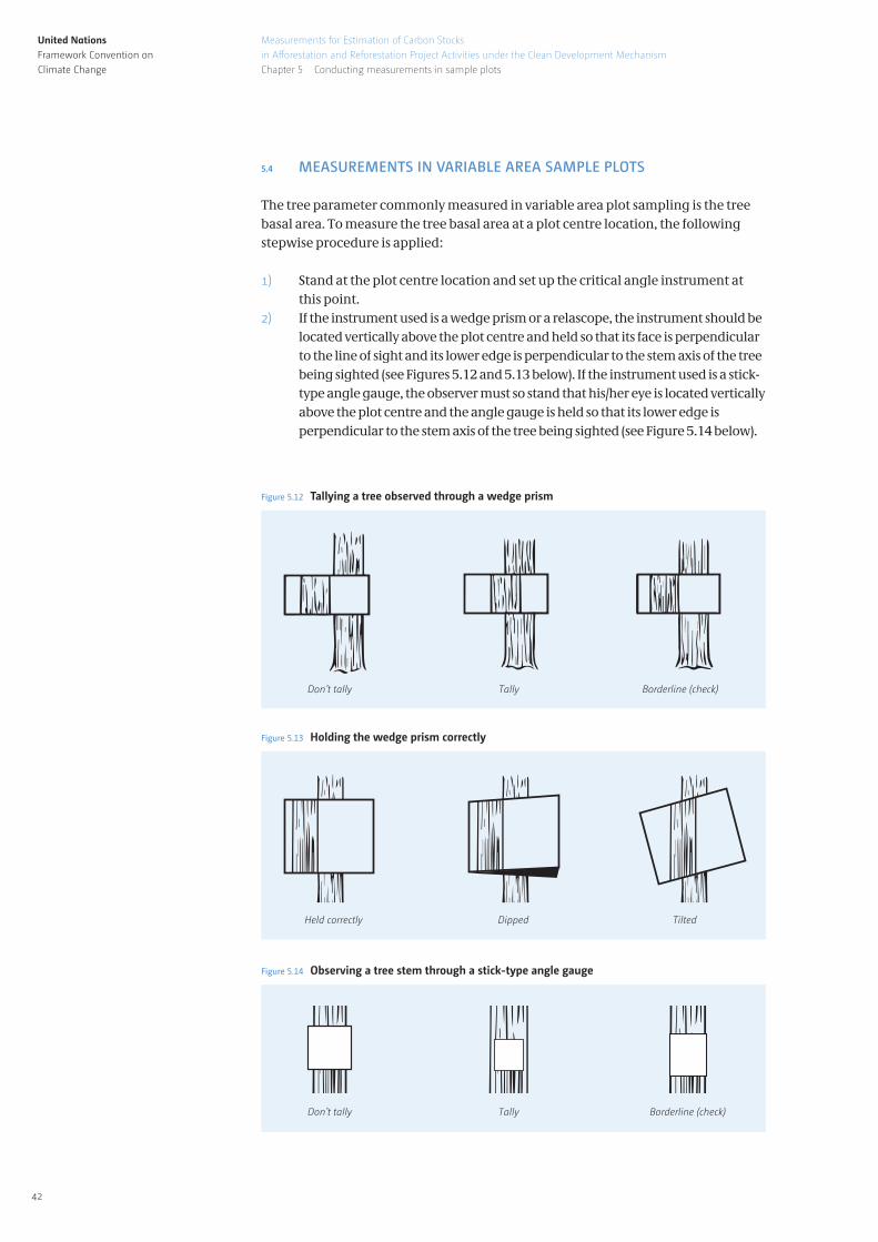
United NationsFramework Convention on Climate Change
42
Measurements for Estimation of Carbon Stocks
in Afforestation and Reforestation Project Activities under the Clean Development Mechanism
Chapter 5 Conducting measurements in sample plots
5 .4 MEASUREMENTS IN VARIABLE AREA SAMPLE PLOTS
The tree parameter commonly measured in variable area plot sampling is the tree basal area. To measure the tree basal area at a plot centre location, the following stepwise procedure is applied:
1) Stand at the plot centre location and set up the critical angle instrument at this point.
2) If the instrument used is a wedge prism or a relascope, the instrument should be located vertically above the plot centre and held so that its face is perpendicular to the line of sight and its lower edge is perpendicular to the stem axis of the tree being sighted (see Figures 5.12 and 5.13 below). If the instrument used is a stick-type angle gauge, the observer must so stand that his/her eye is located vertically above the plot centre and the angle gauge is held so that its lower edge is perpendicular to the stem axis of the tree being sighted (see Figure 5.14 below).
Don’t tally Tally Borderline (check)
Figure 5.12 Tallying a tree observed through a wedge prism
Held correctly Dipped Tilted
Figure 5.13 Holding the wedge prism correctly
Don’t tally Tally Borderline (check)
Figure 5.14 Observing a tree stem through a stick-type angle gauge
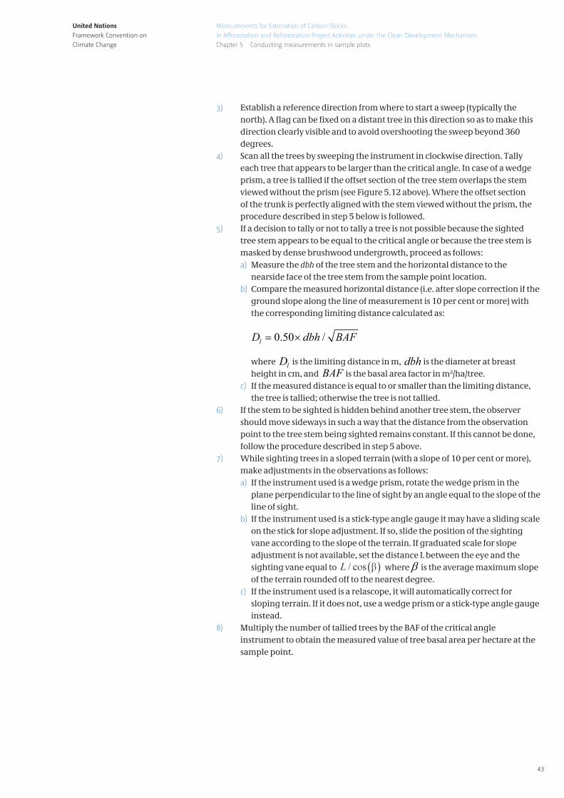
United NationsFramework Convention on Climate Change
43
Measurements for Estimation of Carbon Stocks
in Afforestation and Reforestation Project Activities under the Clean Development Mechanism
Chapter 5 Conducting measurements in sample plots
3) Establish a reference direction from where to start a sweep (typically the north). A flag can be fixed on a distant tree in this direction so as to make this direction clearly visible and to avoid overshooting the sweep beyond 360 degrees.
4) Scan all the trees by sweeping the instrument in clockwise direction. Tally each tree that appears to be larger than the critical angle. In case of a wedge prism, a tree is tallied if the offset section of the tree stem overlaps the stem viewed without the prism (see Figure 5.12 above). Where the offset section of the trunk is perfectly aligned with the stem viewed without the prism, the procedure described in step 5 below is followed.
5) If a decision to tally or not to tally a tree is not possible because the sighted tree stem appears to be equal to the critical angle or because the tree stem is masked by dense brushwood undergrowth, proceed as follows:
a) Measure the dbh of the tree stem and the horizontal distance to the nearside face of the tree stem from the sample point location.
b) Compare the measured horizontal distance (i.e. after slope correction if the ground slope along the line of measurement is 10 per cent or more) with the corresponding limiting distance calculated as:
where lD is the limiting distance in m, dbh is the diameter at breast height in cm, and BAF is the basal area factor in m2/ha/tree.
c) If the measured distance is equal to or smaller than the limiting distance, the tree is tallied; otherwise the tree is not tallied.
6) If the stem to be sighted is hidden behind another tree stem, the observer should move sideways in such a way that the distance from the observation point to the tree stem being sighted remains constant. If this cannot be done, follow the procedure described in step 5 above.
7) While sighting trees in a sloped terrain (with a slope of 10 per cent or more), make adjustments in the observations as follows:
a) If the instrument used is a wedge prism, rotate the wedge prism in the plane perpendicular to the line of sight by an angle equal to the slope of the line of sight.
b) If the instrument used is a stick-type angle gauge it may have a sliding scale on the stick for slope adjustment. If so, slide the position of the sighting vane according to the slope of the terrain. If graduated scale for slope adjustment is not available, set the distance L between the eye and the sighting vane equal to where β is the average maximum slope of the terrain rounded off to the nearest degree.
c) If the instrument used is a relascope, it will automatically correct for sloping terrain. If it does not, use a wedge prism or a stick-type angle gauge instead.
8) Multiply the number of tallied trees by the BAF of the critical angle instrument to obtain the measured value of tree basal area per hectare at the sample point.
0.50 /lD dbh BAF= ×
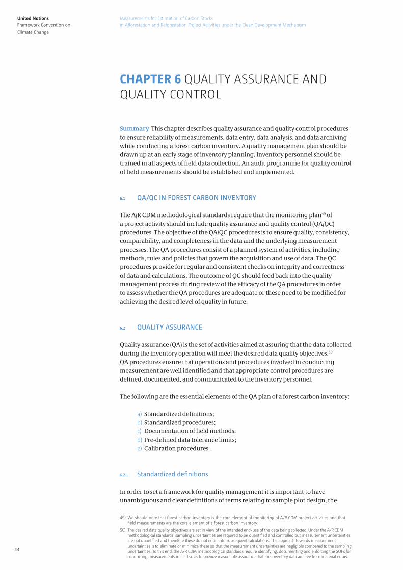
United NationsFramework Convention on Climate Change
44
Measurements for Estimation of Carbon Stocks
in Afforestation and Reforestation Project Activities under the Clean Development Mechanism
CHAPTER 6 QUALITY ASSURANCE AND QUALITY CONTROL
Summary This chapter describes quality assurance and quality control procedures to ensure reliability of measurements, data entry, data analysis, and data archiving while conducting a forest carbon inventory. A quality management plan should be drawn up at an early stage of inventory planning. Inventory personnel should be trained in all aspects of field data collection. An audit programme for quality control of field measurements should be established and implemented.
6 .1 QA/QC IN FOREST CARBON INVENTORY
The A/R CDM methodological standards require that the monitoring plan49 of a project activity should include quality assurance and quality control (QA/QC) procedures. The objective of the QA/QC procedures is to ensure quality, consistency, comparability, and completeness in the data and the underlying measurement processes. The QA procedures consist of a planned system of activities, including methods, rules and policies that govern the acquisition and use of data. The QC procedures provide for regular and consistent checks on integrity and correctness of data and calculations. The outcome of QC should feed back into the quality management process during review of the efficacy of the QA procedures in order to assess whether the QA procedures are adequate or these need to be modified for achieving the desired level of quality in future.
6 .2 QUALITY ASSURANCE
Quality assurance (QA) is the set of activities aimed at assuring that the data collected during the inventory operation will meet the desired data quality objectives.50 QA procedures ensure that operations and procedures involved in conducting measurement are well identified and that appropriate control procedures are defined, documented, and communicated to the inventory personnel.
The following are the essential elements of the QA plan of a forest carbon inventory: a) Standardized definitions; b) Standardized procedures; c) Documentation of field methods; d) Pre-defined data tolerance limits; e) Calibration procedures.
6.2.1 Standardized definitions
In order to set a framework for quality management it is important to have unambiguous and clear definitions of terms relating to sample plot design, the
49) We should note that forest carbon inventory is the core element of monitoring of A/R CDM project activities and that field measurements are the core element of a forest carbon inventory.
50) The desired data quality objectives are set in view of the intended end-use of the data being collected. Under the A/R CDM methodological standards, sampling uncertainties are required to be quantified and controlled but measurement uncertainties are not quantified and therefore these do not enter into subsequent calculations. The approach towards measurement uncertainties is to eliminate or minimize these so that the measurement uncertainties are negligible compared to the sampling uncertainties. To this end, the A/R CDM methodological standards require identifying, documenting and enforcing the SOPs for conducting measurements in field so as to provide reasonable assurance that the inventory data are free from material errors.
United NationsFramework Convention on Climate Change
45
Measurements for Estimation of Carbon Stocks
in Afforestation and Reforestation Project Activities under the Clean Development Mechanism
Chapter 6 Quality assurance and quality control
variables to be measured in a sample plot, and the data quality objectives to be met in measurement of each of these variables.
Definitions related to sample plot designs and the variables to be measured in sample plots have been discussed in the Chapters 4 and 5 of this manual. Project-specific documentation of such definitions should be prepared in a language easily understood by the inventory personnel at the time of a forest carbon inventory.
Definitions related to data quality objectives are discussed below.
Data quality objectives and indicatorsIt is important to clearly define what is meant by data quality, how data quality is to be measured, and what the data quality objectives (i.e. the minimum quality thresholds) are that must be met during the process of inventory data collection.
In the context of conducting forest carbon inventory measurements the following four data quality indicators are relevant:
a) Precision; b) Accuracy; c) Completeness; d) Comparability.
Precision is defined as the measure of agreement among repeated measurements of the same variable under identical or substantially similar conditions. The precision of a measurement depends on the measuring instrument (e.g. the least count and the stability of the instrument) as well as on how the measurements are conducted (e.g. the knowledge, ability, skill, motivation and diligence of the person conducting the measurement).
Precision is estimated by comparing the inventory measurement data with the control measurement data obtained by independently re-measuring a sub-sample of the inventory data. A common statistical estimator of precision is the standard deviation of the pairwise differences between the inventory measurement values and the control measurement values.
Accuracy is a measure of how close the measured value of a variable is to the true value of the variable. The true value of a variable is unknown but in practice it is represented by the value resulting from control measurement.
The quantitative measure of accuracy is represented by bias which is defined as the systematic or persistent deviation of the measured value from the true value.51 Bias is a reverse indicator of accuracy, i.e. the lower the bias, the higher the accuracy of the data. The data quality objective in respect of bias is that the data should be free from bias. In practice, the objective is said to be achieved if the bias is so small that it will not materially affect the desired outcomes resulting from use of the data.
Bias may originate from sources such as calibration errors and incorrect use of measurement methods or equipment.
Completeness is a measure of the amount of usable data obtained from measurement expressed as a percentage of the number of measurement data
51) Note that precision is also defined, like bias, as the difference between the measured value and the control value. What characterizes bias is the systematic or persistent deviation of measured values in one particular direction across a set of measurements or a range within a set of measurements.
United NationsFramework Convention on Climate Change
46
Measurements for Estimation of Carbon Stocks
in Afforestation and Reforestation Project Activities under the Clean Development Mechanism
Chapter 6 Quality assurance and quality control
that should have been obtained according to the sampling design. Completeness indicates how well a sampling plan was implemented.
Although completeness of data is easily expressed as a percentage of the data that should have been obtained, the data quality objective (tolerance threshold) is not easy to prescribe in quantitative terms because the effect of an incomplete dataset entering into analysis will differ greatly from case to case. For example, assume that in a hypothetical stratum a total of 24 sample plots were to be installed and measured. During the inventory, only 20 sample plots were measured because the remaining four plots were found to be inaccessible. Can the incomplete data be analysed and the necessary conclusions drawn about the mean biomass per hectare in the stratum? The answer to this question will depend on how the missing plots are distributed across the stratum. If all four missing sample plots are located on the higher reaches of steep hilly slopes, then the omission of measurements of these plots wills most likely result in significant bias since the average biomass values of the upper slope plots is not likely to be similar to that of the rest of the plots. On the other hand, if these four plots are randomly distributed across the stratum, their omission from measurement should not be a cause for serious concern. For appraisal of completeness of data, it is crucial to determine whether or not the exclusion of a part of data is likely to result in bias in the estimated mean value of the targeted population.
Hence the data quality objective of completeness should be carefully considered on a case-by-case basis by assessing how the absence of the missing data is likely to affect the decision to be made on the basis of originally planned complete set of data.
Comparability is the measure of confidence that two data sets can contribute to common interpretation and analysis of the population parameter of interest. Quantitative measures of comparability can also be generated from statistical tests that measure the similarity or difference between two data sets, but commonly comparability is assessed in qualitative terms alone. For example, in a hypothetical stratum of a forest carbon inventory, the tree dbh was being measured with diameter callipers. The callipers used by one field team broke down in the middle of their work and the remaining dbh measurements had to be conducted with a steel tape graduated to millimetres. Are the two sets of data comparable and amenable to the same analysis? In general, the answer to this question should be yes, since the precision, accuracy and reliability of the two methods of measurements are similar. More generally, one could ask: Are the data from different teams, different strata, and different regions comparable with each other? The answer to this question in general should also be yes if, at the QA stage, adequate measures were taken to ensure that the data from these various sources are comparable.
A description of the four data quality indicators and the associated data quality objectives52 are summarized in Table 6.1 below.
52) The term measurement quality objective is sometimes used instead of the term data quality objective.
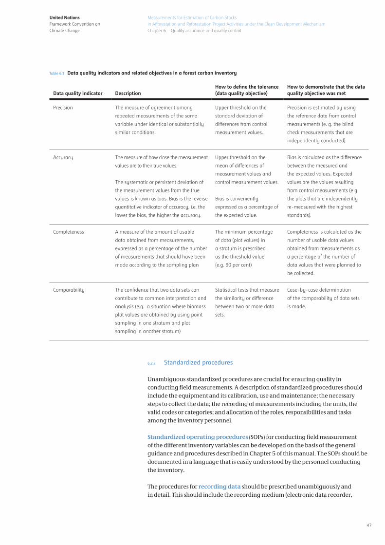
United NationsFramework Convention on Climate Change
47
Measurements for Estimation of Carbon Stocks
in Afforestation and Reforestation Project Activities under the Clean Development Mechanism
Chapter 6 Quality assurance and quality control
Data quality indicator DescriptionHow to define the tolerance(data quality objective)
How to demonstrate that the data quality objective was met
Precision The measure of agreement among
repeated measurements of the same
variable under identical or substantially
similar conditions.
Upper threshold on the
standard deviation of
differences from control
measurement values.
Precision is estimated by using
the reference data from control
measurements (e. g. the blind
check measurements that are
independently conducted).
Accuracy The measure of how close the measurement
values are to their true values.
The systematic or persistent deviation of
the measurement values from the true
values is known as bias. Bias is the reverse
quantitative indicator of accuracy, i.e. the
lower the bias, the higher the accuracy.
Upper threshold on the
mean of differences of
measurement values and
control measurement values.
Bias is conveniently
expressed as a percentage of
the expected value.
Bias is calculated as the difference
between the measured and
the expected values. Expected
values are the values resulting
from control measurements (e g
the plots that are independently
re-measured with the highest
standards).
Completeness A measure of the amount of usable
data obtained from measurements,
expressed as a percentage of the number
of measurements that should have been
made according to the sampling plan
The minimum percentage
of data (plot values) in
a stratum is prescribed
as the threshold value
(e.g. 90 per cent)
Completeness is calculated as the
number of usable data values
obtained from measurements as
a percentage of the number of
data values that were planned to
be collected.
Comparability The confidence that two data sets can
contribute to common interpretation and
analysis (e.g. a situation where biomass
plot values are obtained by using point
sampling in one stratum and plot
sampling in another stratum)
Statistical tests that measure
the similarity or difference
between two or more data
sets.
Case-by-case determination
of the comparability of data sets
is made.
Table 6.1 Data quality indicators and related objectives in a forest carbon inventory
6.2.2 Standardized procedures
Unambiguous standardized procedures are crucial for ensuring quality in conducting field measurements. A description of standardized procedures should include the equipment and its calibration, use and maintenance; the necessary steps to collect the data; the recording of measurements including the units, the valid codes or categories; and allocation of the roles, responsibilities and tasks among the inventory personnel.
Standardized operating procedures (SOPs) for conducting field measurement of the different inventory variables can be developed on the basis of the general guidance and procedures described in Chapter 5 of this manual. The SOPs should be documented in a language that is easily understood by the personnel conducting the inventory.
The procedures for recording data should be prescribed unambiguously and in detail. This should include the recording medium (electronic data recorder,
United NationsFramework Convention on Climate Change
48
Measurements for Estimation of Carbon Stocks
in Afforestation and Reforestation Project Activities under the Clean Development Mechanism
Chapter 6 Quality assurance and quality control
field computer or laptop, paper-based forms, etc.) and the persons responsible for recording and checking. Irrespective of the medium of recording being used, data descriptions (data dictionary) should be specified wherein the units, the valid range of values, and in the case of categorical variables the valid categories, should be specified clearly.
The organization of the roles, responsibilities and tasks among the different teams should be decided in advance and communicated to the inventory personnel since a forest carbon inventory generally requires individuals and teams with skills in different areas of expertise. The principal roles in an inventory team are briefly described below, although the exact organization of the team will depend on the size, complexity and scope of the inventory.
The inventory manager is the person with the overall responsibility for the successful completion of the inventory. An independent, small yet experienced, QC team should remain attached with the inventory manager. The QC team should also assist the manager in conducting training activities.
The field teams are responsible for conducting field measurements in sample plots and transmitting the data to the inventory manager or to the data analysis team. A field data collection team usually consists of a team leader and one or more assistants.
The data analysis team is one or more persons with specific expertise in statistical analysis methods, including expertise in the use of statistical software.53 Although personnel in this team should also be involved in data collection work in order to gain insight into the possible issues related to data quality, their main responsibility should be analysis of data and generation of the required reports.
A suggested organizational set up and distribution of roles and responsibilities of inventory personnel is provided in Table 6.2 below.
53) It is possible that the inventory manager possesses the necessary data analysis skills and remains responsible for analysis of the data. A more formalized organization is more likely to be the case in large and complex inventory projects.
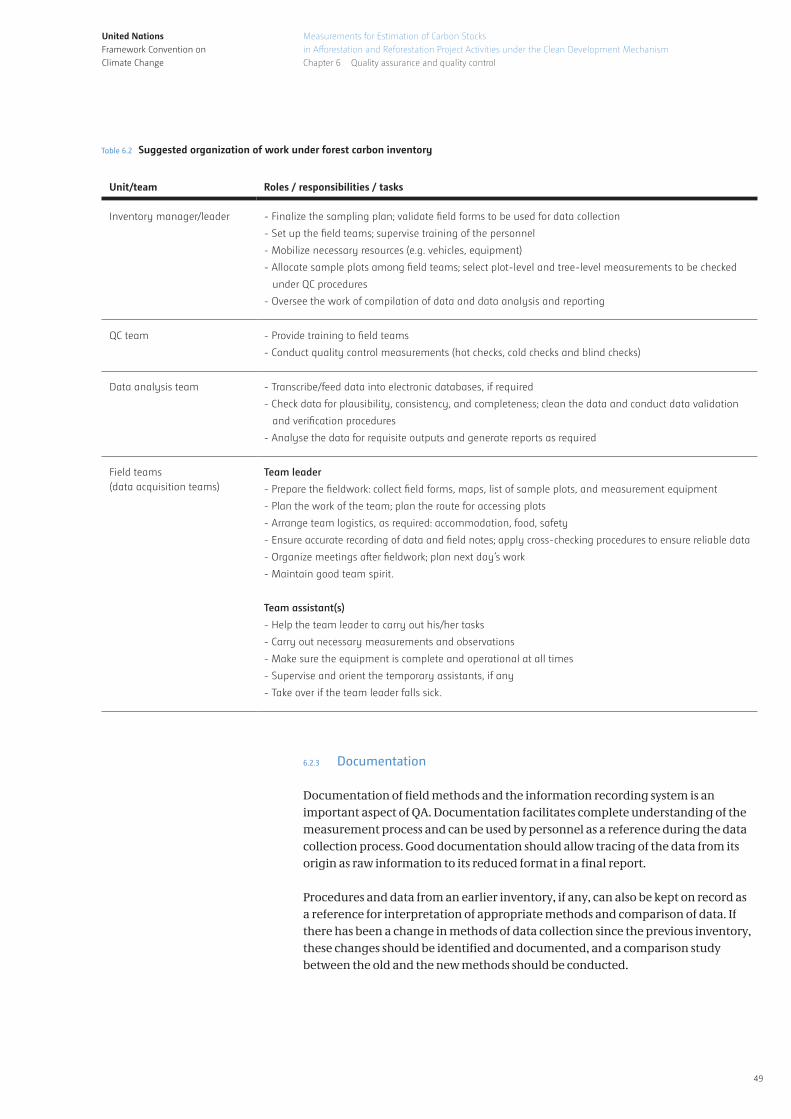
United NationsFramework Convention on Climate Change
49
Measurements for Estimation of Carbon Stocks
in Afforestation and Reforestation Project Activities under the Clean Development Mechanism
Chapter 6 Quality assurance and quality control
Unit/team Roles / responsibilities / tasks
Inventory manager/leader - Finalize the sampling plan; validate field forms to be used for data collection
- Set up the field teams; supervise training of the personnel
- Mobilize necessary resources (e.g. vehicles, equipment)
- Allocate sample plots among field teams; select plot-level and tree-level measurements to be checked
under QC procedures
- Oversee the work of compilation of data and data analysis and reporting
QC team - Provide training to field teams
- Conduct quality control measurements (hot checks, cold checks and blind checks)
Data analysis team - Transcribe/feed data into electronic databases, if required
- Check data for plausibility, consistency, and completeness; clean the data and conduct data validation
and verification procedures
- Analyse the data for requisite outputs and generate reports as required
Field teams (data acquisition teams)
Team leader
- Prepare the fieldwork: collect field forms, maps, list of sample plots, and measurement equipment
- Plan the work of the team; plan the route for accessing plots
- Arrange team logistics, as required: accommodation, food, safety
- Ensure accurate recording of data and field notes; apply cross-checking procedures to ensure reliable data
- Organize meetings after fieldwork; plan next day’s work
- Maintain good team spirit.
Team assistant(s)
- Help the team leader to carry out his/her tasks
- Carry out necessary measurements and observations
- Make sure the equipment is complete and operational at all times
- Supervise and orient the temporary assistants, if any
- Take over if the team leader falls sick.
Table 6.2 Suggested organization of work under forest carbon inventory
6.2.3 Documentation
Documentation of field methods and the information recording system is an important aspect of QA. Documentation facilitates complete understanding of the measurement process and can be used by personnel as a reference during the data collection process. Good documentation should allow tracing of the data from its origin as raw information to its reduced format in a final report.
Procedures and data from an earlier inventory, if any, can also be kept on record as a reference for interpretation of appropriate methods and comparison of data. If there has been a change in methods of data collection since the previous inventory, these changes should be identified and documented, and a comparison study between the old and the new methods should be conducted.
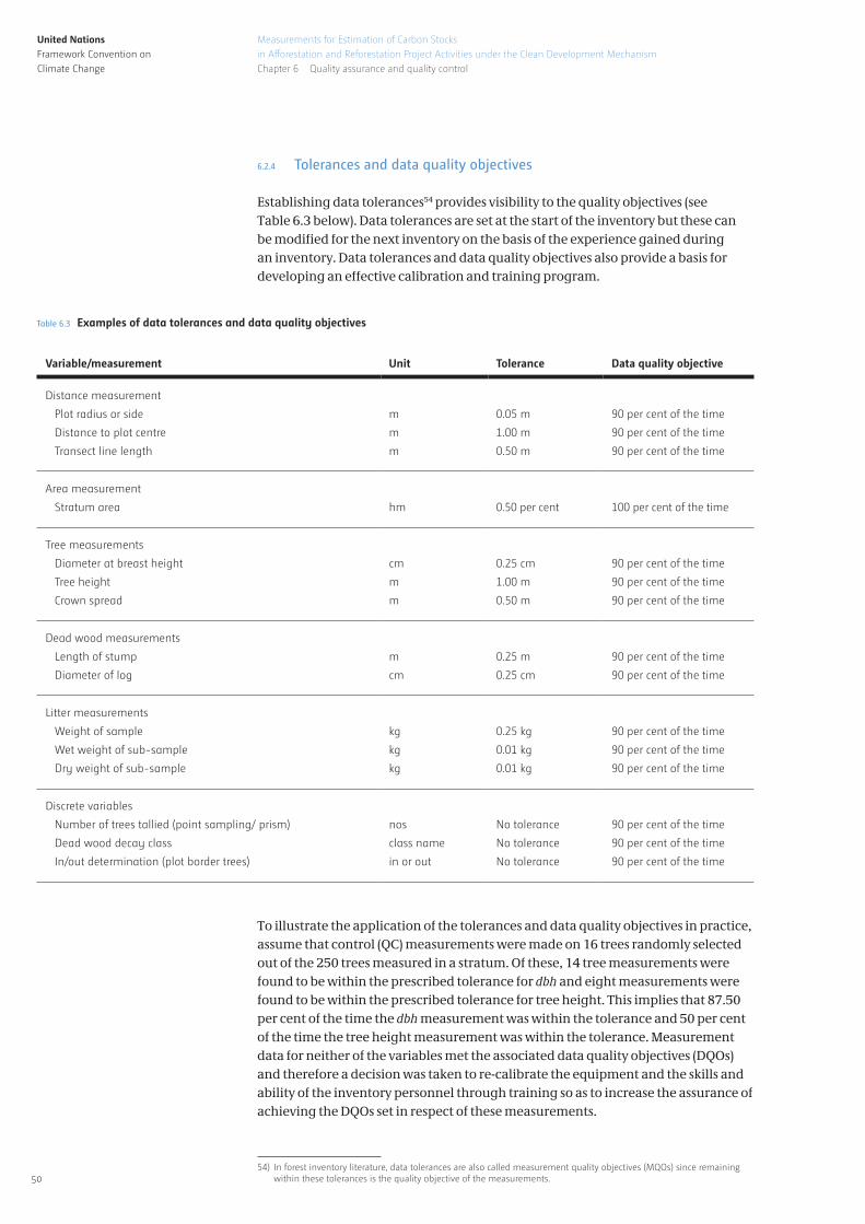
United NationsFramework Convention on Climate Change
50
Measurements for Estimation of Carbon Stocks
in Afforestation and Reforestation Project Activities under the Clean Development Mechanism
Chapter 6 Quality assurance and quality control
6.2.4 Tolerances and data quality objectives
Establishing data tolerances54 provides visibility to the quality objectives (see Table 6.3 below). Data tolerances are set at the start of the inventory but these can be modified for the next inventory on the basis of the experience gained during an inventory. Data tolerances and data quality objectives also provide a basis for developing an effective calibration and training program.
To illustrate the application of the tolerances and data quality objectives in practice, assume that control (QC) measurements were made on 16 trees randomly selected out of the 250 trees measured in a stratum. Of these, 14 tree measurements were found to be within the prescribed tolerance for dbh and eight measurements were found to be within the prescribed tolerance for tree height. This implies that 87.50 per cent of the time the dbh measurement was within the tolerance and 50 per cent of the time the tree height measurement was within the tolerance. Measurement data for neither of the variables met the associated data quality objectives (DQOs) and therefore a decision was taken to re-calibrate the equipment and the skills and ability of the inventory personnel through training so as to increase the assurance of achieving the DQOs set in respect of these measurements.
54) In forest inventory literature, data tolerances are also called measurement quality objectives (MQOs) since remaining within these tolerances is the quality objective of the measurements.
Variable/measurement Unit Tolerance Data quality objective
Distance measurement
Plot radius or side
Distance to plot centre
Transect line length
m
m
m
0.05 m
1.00 m
0.50 m
90 per cent of the time
90 per cent of the time
90 per cent of the time
Area measurement
Stratum area hm 0.50 per cent 100 per cent of the time
Tree measurements
Diameter at breast height
Tree height
Crown spread
cm
m
m
0.25 cm
1.00 m
0.50 m
90 per cent of the time
90 per cent of the time
90 per cent of the time
Dead wood measurements
Length of stump
Diameter of log
m
cm
0.25 m
0.25 cm
90 per cent of the time
90 per cent of the time
Litter measurements
Weight of sample
Wet weight of sub-sample
Dry weight of sub-sample
kg
kg
kg
0.25 kg
0.01 kg
0.01 kg
90 per cent of the time
90 per cent of the time
90 per cent of the time
Discrete variables
Number of trees tallied (point sampling/ prism)
Dead wood decay class
In/out determination (plot border trees)
nos
class name
in or out
No tolerance
No tolerance
No tolerance
90 per cent of the time
90 per cent of the time
90 per cent of the time
Table 6.3 Examples of data tolerances and data quality objectives
United NationsFramework Convention on Climate Change
51
Measurements for Estimation of Carbon Stocks
in Afforestation and Reforestation Project Activities under the Clean Development Mechanism
Chapter 6 Quality assurance and quality control
6.2.5 Calibration
Calibration involves comparison of a measurement instrument or method of unverified accuracy to a measurement instrument or method of known accuracy in order to detect any variation from the required performance specification.
In general, two distinct components of the forest carbon inventory require calibration: measurement equipment and the skills and abilities of the personnel.
Equipment calibrationThe equipment used for measurement must be prepared and calibrated at the beginning of a measurement campaign. The equipment should remain calibrated throughout the process of measurement. Commonly used measurement equipment requiring calibration includes distance measurement tape, diameter callipers, electronic distance measurement device, compass, clinometer, hypsometer, angle prim, relascope, and GPS receiver.
Personnel skill calibrationTraining is an important aspect of calibration of the skill and the ability of the inventory personnel for conducting field measurements. To achieve certification, the field team leaders and assistants should receive training and undergo testing through test measurements under the supervision of the QC team members. Training can proceed in three steps: instruction and explanation of the methodology (class room training); practice session in the field (accompanied by QC team members); and independent assessment of the performance of the field teams by the QC team.
Training is also an opportunity to get feedback from the inventory personnel on the design and implementation of inventory work as well as on the achievability of the data quality objectives within reasonable costs.
6 .3 QUALITY CONTROL
Quality control is the part of quality management focused on fulfilling quality requirements. It comprises the operational aspects mainly concerned with the assessment and appraisal of quality and determination of whether, and to what extent, the quality objectives are being met or have been met.
QC procedures in forest carbon inventory consist of inspections at two levels: field inspections and data inspection.
6.3.1 Field inspections
Field inspections are conducted by a QC team composed of experienced persons whose work is of assured quality so as to justify their measurements as the control (reference) measurements. These inspections serve the dual purpose of controlling, directing and improving the quality of the data collection work in the field and assessment and evaluation of the quality of the data collected. While the first objective is achieved through random inspections called hot checks and cold checks, the latter objective is accomplished through random inspections called blind checks.
United NationsFramework Convention on Climate Change
52
Measurements for Estimation of Carbon Stocks
in Afforestation and Reforestation Project Activities under the Clean Development Mechanism
Chapter 6 Quality assurance and quality control
Hot checks are control inspections aimed at assessing quality at an early stage and taking corrective actions where required. In hot checks the QC team visits randomly selected sample plots and observes the work of the field team during data collection and corrects any errors in the use of measurement methods or equipment or in the data collected. These early checks are also an opportunity for the field teams to provide feedback on the measurement process and equipment.
Cold checks are also mid-campaign inspections carried out on randomly selected sample plots but these are conducted in the absence of the field team responsible for the measurements. A cold check covers a complete set of core variable measurements and can include a full or partial set of other variables. The data resulting from the QC measurements during a cold check are maintained separately from the original data collected by the field team.
Blind checks are end-of-campaign inspections carried out on randomly selected sample plots and are conducted in the absence of the field team responsible for the measurements. The randomly selected check sample plots cover the entire stratum and each plot is fully re-measured by the QC team. The QC team does not have access to the field data collected by the field team (hence the term ‘blind’).
Blind check inspections are not meant to correct or improve the measurement process or the quality of individual plot measurements, but to assess the quality of the inventory data. The outcome of these inspections indicates to what extent the data quality objectives were finally met across the entire set of data collected in a measurement campaign or a stratum. The datasets resulting from the QC measurements and the original field measurements are maintained separately and the discrepancies between the two sets of data are not reconciled.
Re-measurement fractionsThe sampling fraction for test-check inspection can vary (from a few per cent to over 10 per cent) depending on the importance of a variable in the final outcome of carbon stock estimation. For example, tree dbh and tree height measurements can be checked at higher intensity than the checks on dead wood decay class, or litter weight measurements.
In general, QC measurements should aim for extensive coverage (wide probe) as well as intensive coverage (deep probe) of the inventory measurements. An example of extensive coverage could be the check measurements on the dbh data of trees randomly selected across sample plots spread over the stratum. An example of intensive coverage could be the check measurements on the entire plot data of randomly selected sample plots across the stratum.
6.3.2 Data inspection
Data inspections (also called data audits) consist of data validation and data verification. Data validation is process that evaluates the data independently of the methodological, procedural or compliance standards. It includes screening for plausibility of data and detection of potential deficiencies or bias. Many of the data validation checks are built into the portable data recorder equipment and software which greatly helps in preserving data quality.

United NationsFramework Convention on Climate Change
53
Measurements for Estimation of Carbon Stocks
in Afforestation and Reforestation Project Activities under the Clean Development Mechanism
Chapter 6 Quality assurance and quality control
Data verification is the process of evaluating the completeness, correctness, and compliance of the data set against the prescribed quality standards. Some data verification checks can be developed on the basis of statistical analysis. For example, tree level field measurement data can be checked for errors by visualizing the data through scatter plots (e.g. dbh versus tree height plots) and looking for outliers that appear to be improbable. Such outliers should be flagged and if possible the measurements should be re-checked in field. If field checking is not possible, outlier data should be omitted from calculations so as to maintain a conservative estimate of carbon stocks. Stratum boundaries and corners as well as sample plot locations can be checked against current high resolution satellite data if available.
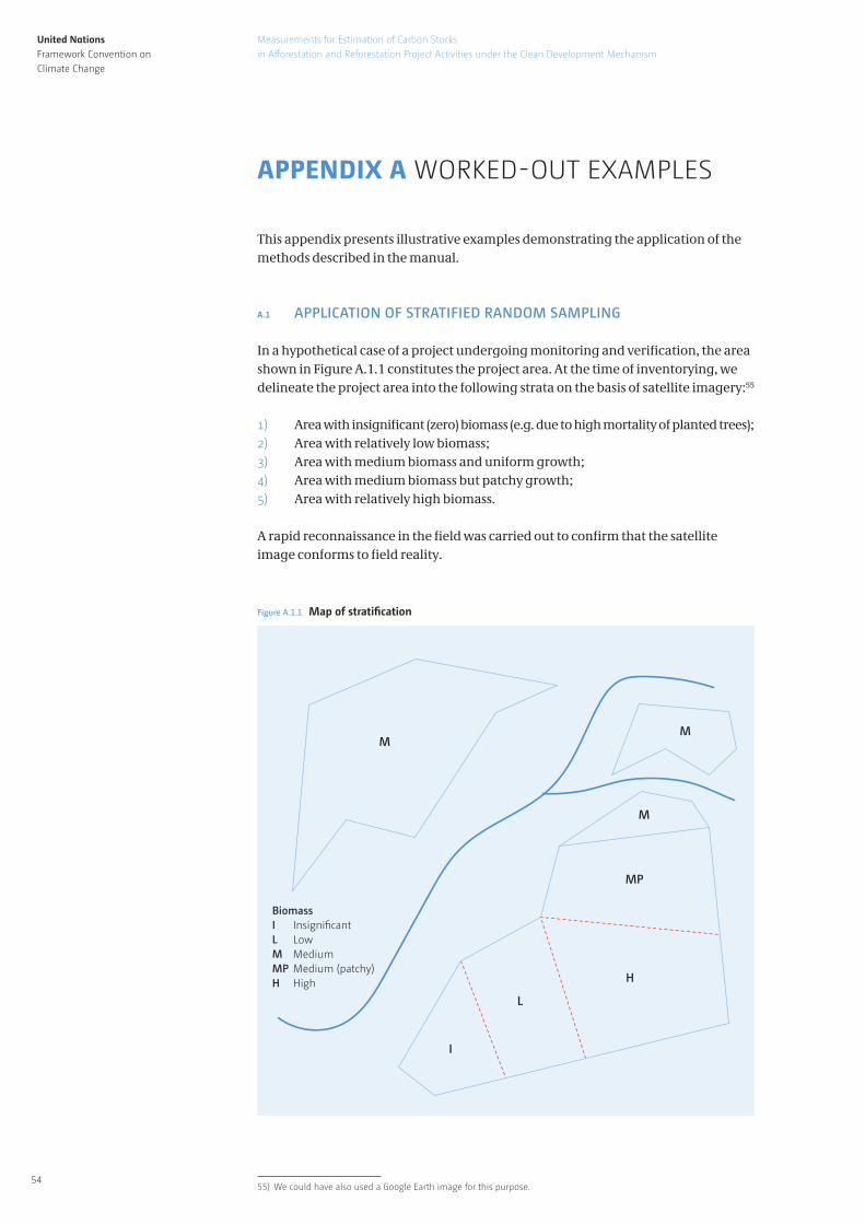
United NationsFramework Convention on Climate Change
54
Measurements for Estimation of Carbon Stocks
in Afforestation and Reforestation Project Activities under the Clean Development Mechanism
APPENDIX A WORKED-OUT EXAMPLES
This appendix presents illustrative examples demonstrating the application of the methods described in the manual.
A .1 APPLICATION OF STRATIFIED RANDOM SAMPLING
In a hypothetical case of a project undergoing monitoring and verification, the area shown in Figure A.1.1 constitutes the project area. At the time of inventorying, we delineate the project area into the following strata on the basis of satellite imagery:55
1) Area with insignificant (zero) biomass (e.g. due to high mortality of planted trees);2) Area with relatively low biomass;3) Area with medium biomass and uniform growth; 4) Area with medium biomass but patchy growth;5) Area with relatively high biomass.
A rapid reconnaissance in the field was carried out to confirm that the satellite image conforms to field reality.
55) We could have also used a Google Earth image for this purpose.
MM
M
MP
H
L
I
BiomassILMMPH
Insigni�cantLowMediumMedium (patchy)High
Figure A.1.1 Map of strati�cation
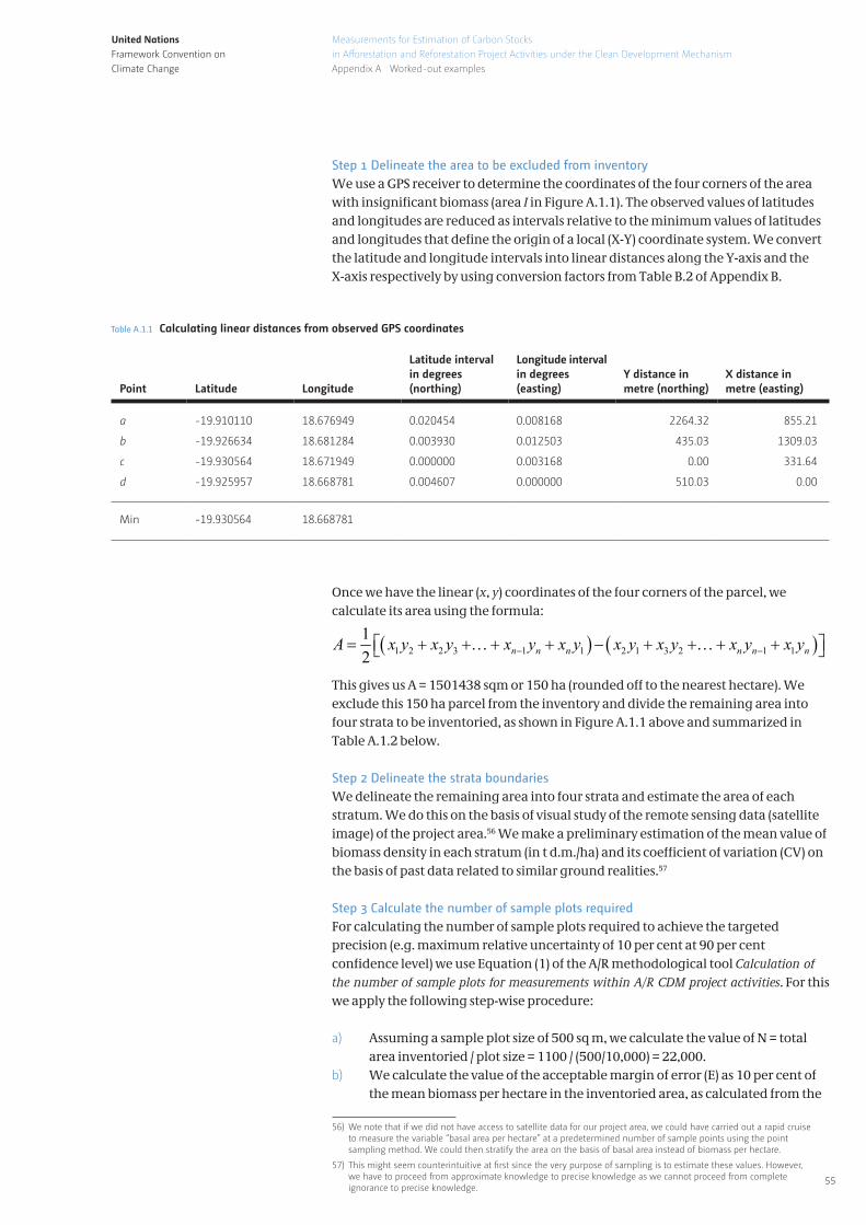
United NationsFramework Convention on Climate Change
55
Measurements for Estimation of Carbon Stocks
in Afforestation and Reforestation Project Activities under the Clean Development Mechanism
Appendix A Worked-out examples
Step 1 Delineate the area to be excluded from inventoryWe use a GPS receiver to determine the coordinates of the four corners of the area with insignificant biomass (area I in Figure A.1.1). The observed values of latitudes and longitudes are reduced as intervals relative to the minimum values of latitudes and longitudes that define the origin of a local (X-Y) coordinate system. We convert the latitude and longitude intervals into linear distances along the Y-axis and the X-axis respectively by using conversion factors from Table B.2 of Appendix B.
Once we have the linear (x, y) coordinates of the four corners of the parcel, we calculate its area using the formula:
This gives us A = 1501438 sqm or 150 ha (rounded off to the nearest hectare). We exclude this 150 ha parcel from the inventory and divide the remaining area into four strata to be inventoried, as shown in Figure A.1.1 above and summarized in Table A.1.2 below.
Step 2 Delineate the strata boundariesWe delineate the remaining area into four strata and estimate the area of each stratum. We do this on the basis of visual study of the remote sensing data (satellite image) of the project area.56 We make a preliminary estimation of the mean value of biomass density in each stratum (in t d.m./ha) and its coefficient of variation (CV) on the basis of past data related to similar ground realities.57
Step 3 Calculate the number of sample plots requiredFor calculating the number of sample plots required to achieve the targeted precision (e.g. maximum relative uncertainty of 10 per cent at 90 per cent confidence level) we use Equation (1) of the A/R methodological tool Calculation of the number of sample plots for measurements within A/R CDM project activities. For this we apply the following step-wise procedure:
a) Assuming a sample plot size of 500 sq m, we calculate the value of N = total area inventoried / plot size = 1100 / (500/10,000) = 22,000.
b) We calculate the value of the acceptable margin of error (E) as 10 per cent of the mean biomass per hectare in the inventoried area, as calculated from the
56) We note that if we did not have access to satellite data for our project area, we could have carried out a rapid cruise to measure the variable “basal area per hectare” at a predetermined number of sample points using the point sampling method. We could then stratify the area on the basis of basal area instead of biomass per hectare.
57) This might seem counterintuitive at first since the very purpose of sampling is to estimate these values. However, we have to proceed from approximate knowledge to precise knowledge as we cannot proceed from complete ignorance to precise knowledge.
Point Latitude Longitude
Latitude interval in degrees(northing)
Longitude interval in degrees(easting)
Y distance in metre (northing)
X distance in metre (easting)
a
b
c
d
-19.910110
-19.926634
-19.930564
-19.925957
18.676949
18.681284
18.671949
18.668781
0.020454
0.003930
0.000000
0.004607
0.008168
0.012503
0.003168
0.000000
2264.32
435.03
0.00
510.03
855.21
1309.03
331.64
0.00
Min -19.930564 18.668781
Table A.1.1 Calculating linear distances from observed GPS coordinates
( ) ( )1 2 2 3 1 1 2 1 3 2 1 112 n n n n n nA x y x y x y x y x y x y x y x y− − = + +…+ + − + +…+ +
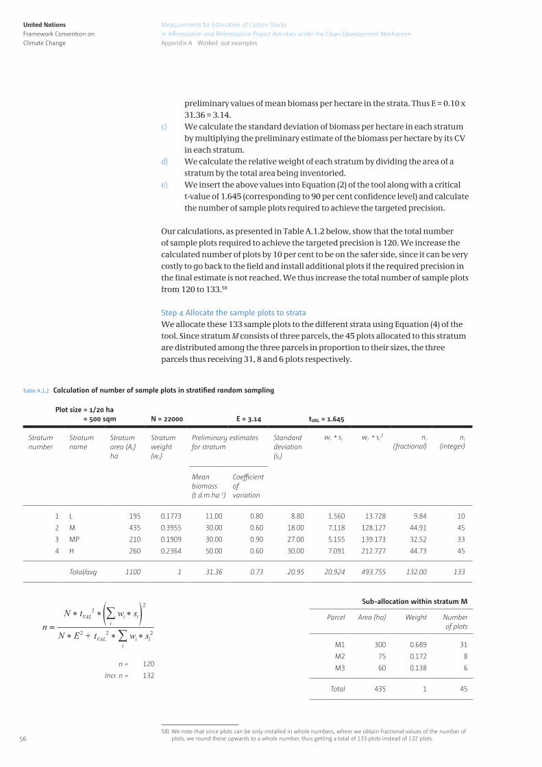
United NationsFramework Convention on Climate Change
56
Measurements for Estimation of Carbon Stocks
in Afforestation and Reforestation Project Activities under the Clean Development Mechanism
Appendix A Worked-out examples
preliminary values of mean biomass per hectare in the strata. Thus E = 0.10 x 31.36 = 3.14.
c) We calculate the standard deviation of biomass per hectare in each stratum by multiplying the preliminary estimate of the biomass per hectare by its CV in each stratum.
d) We calculate the relative weight of each stratum by dividing the area of a stratum by the total area being inventoried.
e) We insert the above values into Equation (2) of the tool along with a critical t-value of 1.645 (corresponding to 90 per cent confidence level) and calculate the number of sample plots required to achieve the targeted precision.
Our calculations, as presented in Table A.1.2 below, show that the total number of sample plots required to achieve the targeted precision is 120. We increase the calculated number of plots by 10 per cent to be on the safer side, since it can be very costly to go back to the field and install additional plots if the required precision in the final estimate is not reached. We thus increase the total number of sample plots from 120 to 133.58
Step 4 Allocate the sample plots to strataWe allocate these 133 sample plots to the different strata using Equation (4) of the tool. Since stratum M consists of three parcels, the 45 plots allocated to this stratum are distributed among the three parcels in proportion to their sizes, the three parcels thus receiving 31, 8 and 6 plots respectively.
58) We note that since plots can be only installed in whole numbers, where we obtain fractional values of the number of plots, we round these upwards to a whole number, thus getting a total of 133 plots instead of 132 plots.
Plot size = 1/20 ha = 500 sqm N = 22000 E = 3 .14 tVAL = 1 .645
Stratum number
Stratum name
Stratum area (Ai)ha
Stratum weight (wi)
Preliminary estimates for stratum
Standard deviation (si )
wi * si wi * si2 ni
( fractional)ni
(integer)
Mean biomass (t d.m.ha-1)
Coefficientofvariation
1
2
3
4
L
M
MP
H
195
435
210
260
0.1773
0.3955
0.1909
0.2364
11.00
30.00
30.00
50.00
0.80
0.60
0.90
0.60
8.80
18.00
27.00
30.00
1.560
7.118
5.155
7.091
13.728
128.127
139.173
212.727
9.84
44.91
32.52
44.73
10
45
33
45
Total/avg 1100 1 31.36 0.73 20.95 20.924 493.755 132.00 133
Table A.1.2 Calculation of number of sample plots in stratified random sampling
Sub-allocation within stratum M
Parcel Area (ha) Weight Number of plots
M1
M2
M3
300
75
60
0.689
0.172
0.138
31
8
6
Total 435 1 45
n = 120
Incr. n = 132
n =N * E2 + tVAL
2 * ∑ wi * si2
i
N * tVAL2 * ∑ wi * si
2
i( (
United NationsFramework Convention on Climate Change
57
Measurements for Estimation of Carbon Stocks
in Afforestation and Reforestation Project Activities under the Clean Development Mechanism
Appendix A Worked-out examples
A .2 APPLICATION OF DOUBLE SAMPLING
At the time of inventorying of carbon stocks in the hypothetical project described in example A.1, we note that the stratum MP (area 210 ha) shows highly patchy growth so that it is not evident how to delineate biomass strata with uniform biomass per hectare values at any spatial scale within this stratum. We therefore decide to adopt the design of double sampling for this stratum.
Step 1 Select the auxiliary variable and measure it in the first-phase sampleWe know that the variables basal area per hectare and tree biomass per hectare are linearly correlated. We decide to measure the auxiliary variable basal area per hectare in a first-phase sample of 100 sample plots. We do this by using the point sampling method. Measurement of basal area by using point sampling method costs only a fraction of the cost of measurement of biomass in sample plots.59
Step 2 Measure the target variable in the second-phase sampleIn the second-phase, we draw a random sample of 15 sample plots from the first-phase sample and we measure the tree diameters in these plots and estimate tree biomass per hectare in each of these plots.
Step 3 Regress the target variable against the auxiliary variable We then perform linear regression between the biomass values and the basal area values of the sample plots in the second-phase sample. The results of regression are summarized in Table A.2.1 below.
Step 4 Adjust mean of the target variable Using Equation (18) of the A/R CDM methodological tool Estimation of carbon stocks and change in carbon stocks of trees and shrubs in A/R CDM project activities, we calculate the adjusted mean of tree biomass per hectare values. The results of adjustment are summarized in Table A.2.2 below.
59) Note that by “measurement of the tree biomass in a sample plot” we mean measurement of the dbh and height of the trees in the sample plot and conversion of these measurement values into per hectare tree biomass in the plot.
Coefficient of regression:
Slope of regression line:
Intercept of regression line:
0.9342
8.4164
-44.2809
Table A.2.1 Regression of auxiliary variable against the target variable
Mean basal area from first-phase sample:
Mean basal area from second-phase sample:
Mean biomass per hectare from second-phase sample:
Mean biomass per hectare adjusted on the basis of regression:
21.34
20.40
127.41
135.32
Table A.2.2 Adjusted mean of the targeted variable
Step 5 Update the uncertainty of the mean Using Equation (19) of the A/R CDM methodological tool Estimation of carbon stocks and change in carbon stocks of trees and shrubs in A/R CDM project activities, we update the uncertainty of the mean tree biomass. Our data, calculations and results are laid out in Table A.2.3 below.
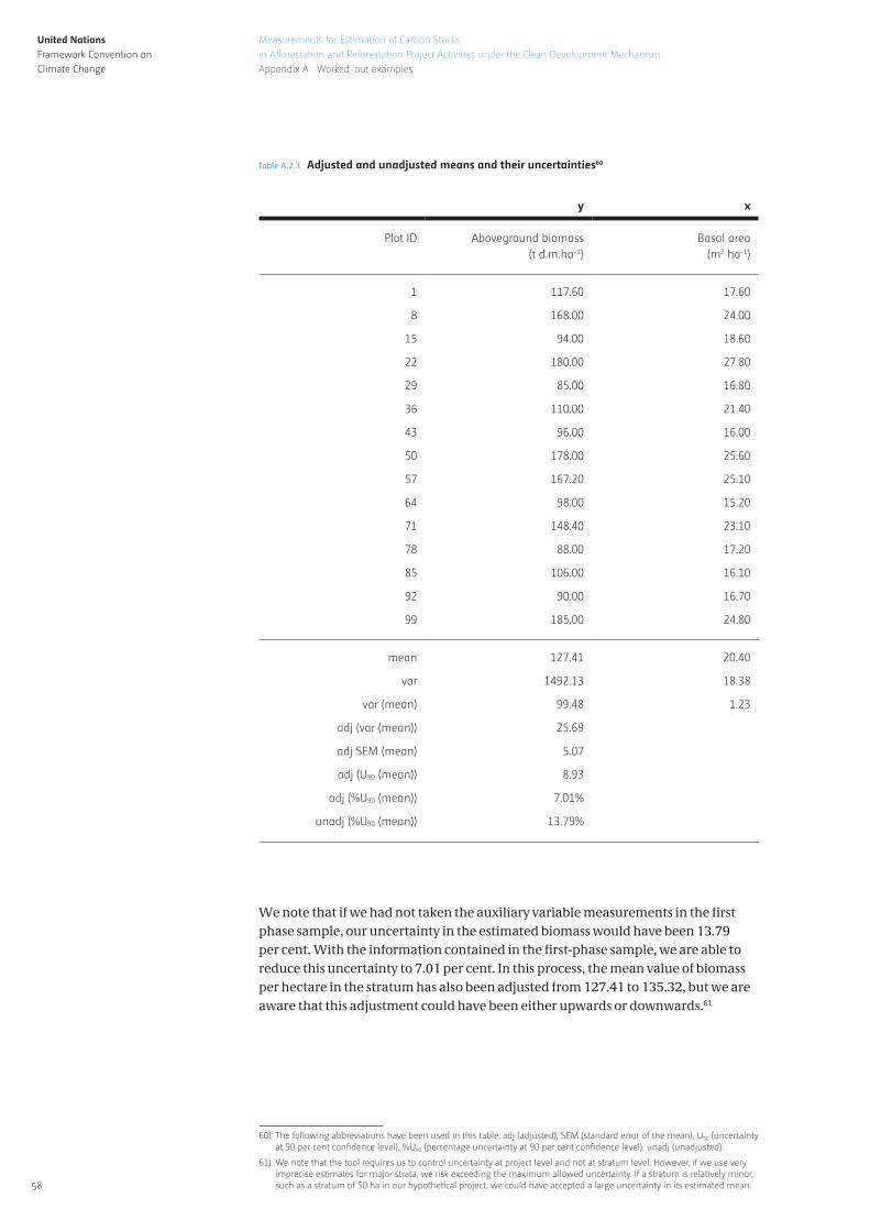
United NationsFramework Convention on Climate Change
58
Measurements for Estimation of Carbon Stocks
in Afforestation and Reforestation Project Activities under the Clean Development Mechanism
Appendix A Worked-out examples
We note that if we had not taken the auxiliary variable measurements in the first phase sample, our uncertainty in the estimated biomass would have been 13.79 per cent. With the information contained in the first-phase sample, we are able to reduce this uncertainty to 7.01 per cent. In this process, the mean value of biomass per hectare in the stratum has also been adjusted from 127.41 to 135.32, but we are aware that this adjustment could have been either upwards or downwards.61
y x
Plot ID Aboveground biomass(t d.m.ha-1)
Basal area(m2 ha-1)
1
8
15
22
29
36
43
50
57
64
71
78
85
92
99
117.60
168.00
94.00
180.00
85.00
110.00
96.00
178.00
167.20
98.00
148.40
88.00
106.00
90.00
185.00
17.60
24.00
18.60
27.80
16.80
21.40
16.00
25.60
25.10
15.20
23.10
17.20
16.10
16.70
24.80
mean
var
var (mean)
adj (var (mean))
adj SEM (mean)
adj (U90 (mean))
adj (%U90 (mean))
unadj (%U90 (mean))
127.41
1492.13
99.48
25.69
5.07
8.93
7.01%
13.79%
20.40
18.38
1.23
Table A.2.3 Adjusted and unadjusted means and their uncertainties60
60) The following abbreviations have been used in this table: adj (adjusted), SEM (standard error of the mean), U90 (uncertainty at 90 per cent confidence level), %U90 (percentage uncertainty at 90 per cent confidence level), unadj (unadjusted).
61) We note that the tool requires us to control uncertainty at project level and not at stratum level. However, if we use very imprecise estimates for major strata, we risk exceeding the maximum allowed uncertainty. If a stratum is relatively minor, such as a stratum of 50 ha in our hypothetical project, we could have accepted a large uncertainty in its estimated mean.
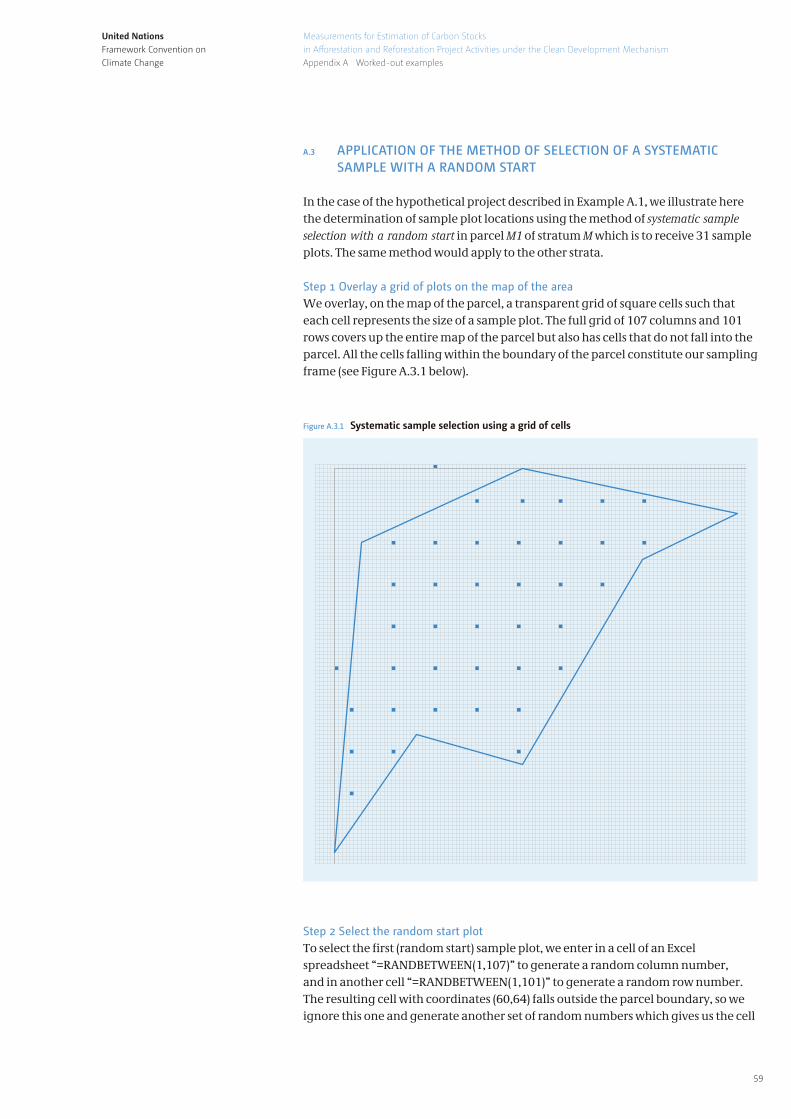
United NationsFramework Convention on Climate Change
59
Measurements for Estimation of Carbon Stocks
in Afforestation and Reforestation Project Activities under the Clean Development Mechanism
Appendix A Worked-out examples
A .3 APPLICATION OF THE METHOD OF SELECTION OF A SYSTEMATIC SAMPLE WITH A RANDOM START
In the case of the hypothetical project described in Example A.1, we illustrate here the determination of sample plot locations using the method of systematic sample selection with a random start in parcel M1 of stratum M which is to receive 31 sample plots. The same method would apply to the other strata.
Step 1 Overlay a grid of plots on the map of the area We overlay, on the map of the parcel, a transparent grid of square cells such that each cell represents the size of a sample plot. The full grid of 107 columns and 101 rows covers up the entire map of the parcel but also has cells that do not fall into the parcel. All the cells falling within the boundary of the parcel constitute our sampling frame (see Figure A.3.1 below).
Step 2 Select the random start plot To select the first (random start) sample plot, we enter in a cell of an Excel spreadsheet “=RANDBETWEEN(1,107)” to generate a random column number, and in another cell “=RANDBETWEEN(1,101)” to generate a random row number. The resulting cell with coordinates (60,64) falls outside the parcel boundary, so we ignore this one and generate another set of random numbers which gives us the cell
Figure A.3.1 Systematic sample selection using a grid of cells
United NationsFramework Convention on Climate Change
60
Measurements for Estimation of Carbon Stocks
in Afforestation and Reforestation Project Activities under the Clean Development Mechanism
Appendix A Worked-out examples
with the coordinates (87, 56) which again falls outside the parcel. We repeat this process and we get the cell coordinates of (27, 53) and this cell falls inside the parcel. This is our first (random start) sample plot.62
Step 3 Determine the plot selection interval and select the sample plotsWe now determine the X-axis and Y-axis intervals between two plots considering that we want the 31 sample plots to be evenly spread over the parcel. We calculate the value SQRT(6000/31) in Excel because with our plot size of one-twentieth of a hectare, the parcel area will accommodate a total of 6000 plots. The square root is needed because we need two equal intervals, one along the X-axis and the other along the Y-axis. This gives us an interval of 13. Using this interval, we select every 13th plot starting from the first (randomly selected) sample plot along the X-axis and likewise every 13th plot along the Y-axis until we reach the parcel boundary in each direction. We find that we can accommodate only 28 plots in this manner and therefore we downsize the interval to 12 and then re-select the plot locations and we get 34 plots which we accept.63
Step 4 Locate the sample plots on the groundIf we knew the georeferenced coordinates (e.g. the latitude and longitude) of one of these plots, we could have calculated the coordinates of all the sample plot centres and by feeding these coordinates into a GPS receiver we would be able to locate the plot centres in the field.
Step 5 Insert additional sample plots (optional)If, after conducting the inventory, we discover that we have not met the required precision and we need to install additional sample plots, we could use a similar method for insertion of additional sample plots in between these plots. For example, by joining all the plot centres we divide the stratum into a grid of 30 cells. To add 10 additional plots we will randomly select the first cell and then select every third cell in either direction. The centres of these cells will give us the locations of the additional sample plots.
62) We are aware that this somewhat elaborate process of selection of the starting cell can be substituted by subjectively picking a random cell inside the map. The only difference would be that while the process we followed is an objective process and therefore is verifiable, in the case of a subjective choice it will not be possible for a third party to verify the choice of the starting cell.
63) We understand that the sample size is not a requirement in itself; it is a means of assuring that the uncertainty in our estimate of carbon stocks will remain within the maximum allowable limit. The A/R CDM standards prescribe the requirements in terms of the maximum allowable uncertainty. As long as we can demonstrate that the uncertainty of our estimation does not exceed the maximum allowable uncertainty, the number of sample plots can somewhat exceed or fall short of the number calculated from the tool.
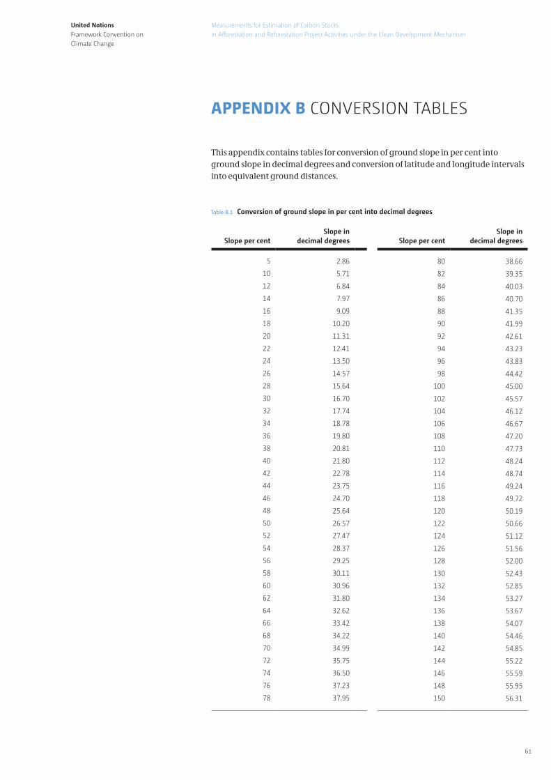
United NationsFramework Convention on Climate Change
61
Measurements for Estimation of Carbon Stocks
in Afforestation and Reforestation Project Activities under the Clean Development Mechanism
APPENDIX B CONVERSION TABLES
This appendix contains tables for conversion of ground slope in per cent into ground slope in decimal degrees and conversion of latitude and longitude intervals into equivalent ground distances.
Slope per centSlope in
decimal degrees Slope per centSlope in
decimal degrees
5
10
12
14
16
18
20
22
24
26
28
30
32
34
36
38
40
42
44
46
48
50
52
54
56
58
60
62
64
66
68
70
72
74
76
78
2.86
5.71
6.84
7.97
9.09
10.20
11.31
12.41
13.50
14.57
15.64
16.70
17.74
18.78
19.80
20.81
21.80
22.78
23.75
24.70
25.64
26.57
27.47
28.37
29.25
30.11
30.96
31.80
32.62
33.42
34.22
34.99
35.75
36.50
37.23
37.95
80
82
84
86
88
90
92
94
96
98
100
102
104
106
108
110
112
114
116
118
120
122
124
126
128
130
132
134
136
138
140
142
144
146
148
150
38.66
39.35
40.03
40.70
41.35
41.99
42.61
43.23
43.83
44.42
45.00
45.57
46.12
46.67
47.20
47.73
48.24
48.74
49.24
49.72
50.19
50.66
51.12
51.56
52.00
52.43
52.85
53.27
53.67
54.07
54.46
54.85
55.22
55.59
55.95
56.31
Table B.1 Conversion of ground slope in per cent into decimal degrees
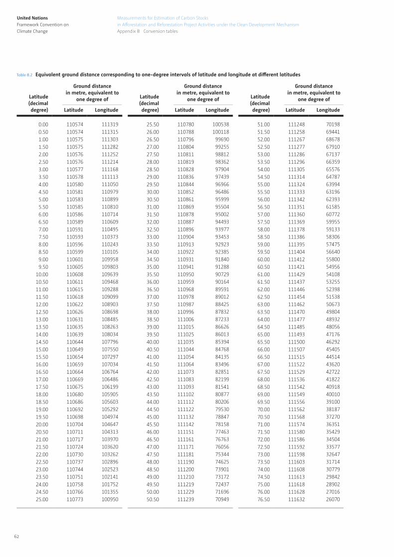
United NationsFramework Convention on Climate Change
62
Measurements for Estimation of Carbon Stocks
in Afforestation and Reforestation Project Activities under the Clean Development Mechanism
Appendix B Conversion tables
Table B.2 Equivalent ground distance corresponding to one-degree intervals of latitude and longitude at different latitudes
Latitude(decimal degree) Latitude Longitude
0.000.501.001.502.002.503.003.504.004.505.005.506.006.507.007.508.008.509.009.50
10.0010.5011.0011.5012.0012.5013.0013.5014.0014.5015.0015.5016.0016.5017.0017.5018.0018.5019.0019.5020.0020.5021.0021.5022.0022.5023.0023.5024.0024.5025.00
110574110574110575110575110576110576110577110578110580110581110583110585110586110589110591110593110596110599110601110605110608110611110615110618110622110626110631110635110639110644110649110654110659110664110669110675110680110686110692110698110704110711110717110724110730110737110744110751110758110766110773
111319111315111303111282111252111214111168111113111050110979110899110810110714110609110495110373110243110105109958109803109639109468109288109099108903108698108485108263108034107796107550107297107034106764106486106199105905105603105292104974104647104313103970103620103262102896102523102141101752101355100950
Ground distancein metre, equivalent to
one degree of Latitude(decimal degree) Latitude Longitude
51.0051.5052.0052.5053.0053.5054.0054.5055.0055.5056.0056.5057.0057.5058.0058.5059.0059.5060.0060.5061.0061.5062.0062.5063.0063.5064.0064.5065.0065.5066.0066.5067.0067.5068.0068.5069.0069.5070.0070.5071.0071.5072.0072.5073.0073.5074.0074.5075.0076.0076.50
111248111258111267111277111286111296111305111314111324111333111342111351111360111369111378111386111395111404111412111421111429111437111446111454111462111470111477111485111493111500111507111515111522111529111536111542111549111556111562111568111574111580111586111592111598111603111608111613111618111628111632
701986944168678679106713766359655766478763994631966239361585607725995559133583065747556640558005495654108532555239851538506734980448932480564717646292454054451443620427224182240918400103910038187372703635135429345043357732647317143077929842289022701626070
Ground distancein metre, equivalent to
one degree ofLatitude(decimal degree) Latitude Longitude
25.5026.0026.5027.0027.5028.0028.5029.0029.5030.0030.5031.0031.5032.0032.5033.0033.5034.0034.5035.0035.5036.0036.5037.0037.5038.0038.5039.0039.5040.0040.5041.0041.5042.0042.5043.0043.5044.0044.5045.0045.5046.0046.5047.0047.5048.0048.5049.0049.5050.0050.50
110780110788110796110804110811110819110828110836110844110852110861110869110878110887110896110904110913110922110931110941110950110959110968110978110987110996111006111015111025111035111044111054111064111073111083111093111102111112111122111132111142111151111161111171111181111190111200111210111219111229111239
10053810011899690992559881298362979049743996966964869599995504950029449393977934539292392385918409128890729901648959189012884258783287233866268601385394847688413583496828518219981541808778020679530788477815877463767637605675344746257390173172724377169670949
Ground distancein metre, equivalent to
one degree of
United NationsFramework Convention on Climate Change
63
Measurements for Estimation of Carbon Stocks
in Afforestation and Reforestation Project Activities under the Clean Development Mechanism
APPENDIX C GLOSSARY OF CDM TERMS
This appendix contains definition of CDM terms relating to A/R project activities. The user may wish to refer to the full official Glossary of CDM terms64 for a more complete collection of CDM terms and definitions.
Actual net GHG removals by sinks The sum of the verifiable changes in carbon stocks in the carbon pools within a project boundary that are attributable to an A/R or SSC A/R CDM project activity or PoA (A/R), as applicable, minus any increase in anthropogenic GHG emissions by sources (measured in carbon dioxide equivalents) within the project boundary that is caused by the implementation of the A/R or SSC A/R CDM project activity or PoA (A/R), as applicable.
AfforestationThe direct human-induced conversion of land that has not been forested for a period of at least 50 years to forested land through planting, seeding and/or human-induced promotion of natural seed sources.
A/R CDM project activityAn afforestation or reforestation measure, operation or action that aims to achieve net anthropogenic GHG removals by sinks, whether as a whole project or as a part of a project.
Baseline net GHG removals by sinksThe sum of the changes in carbon stocks in the carbon pools within the project boundary that would have occurred in the absence of the A/R or SSC A/R CDM project activity or PoA (A/R).
Carbon poolsAbove-ground biomass, below-ground biomass, litter, dead wood and soil organic carbon.
CPA (component project activity)A single measure, or a set of interrelated measures under a PoA, to reduce GHG emissions by sources or result in net anthropogenic GHG removals by sinks, applied within a designated area defined in the baseline methodology(ies).
DNA (designated national authority)The body granted responsibility by a Party, among other things and where applicable, to issue a letter of approval with respect to CDM project activities or PoAs on behalf of that Party, in accordance with the CDM rules and requirements.
DOE (designated operational entity)An entity designated by the CMP, based on a recommendation by the Board, as qualified to validate proposed CDM project activities and PoAs, as well as verify and certify reductions in anthropogenic emissions by sources of GHG and net anthropogenic GHG removals by sinks.
Eligibility of landThe determination of which land meets the conditions required to be included in an
64) Available at <http://cdm.unfccc.int/Reference/Guidclarif/glos_CDM.pdf>
United NationsFramework Convention on Climate Change
64
Measurements for Estimation of Carbon Stocks
in Afforestation and Reforestation Project Activities under the Clean Development Mechanism
Appendix C Glossary of CDM terms
A/R or SSC A/R CDM project activity or PoA (A/R), in accordance with the CDM rules and requirements.
Forest“Forest” is a minimum area of land of 0.05–1.0 hectare with tree crown cover (or equivalent stocking level) of more than 10–30 per cent with trees with the potential to reach a minimum height of 2–5 metres at maturity in situ. A forest may consist either of closed forest formations where trees of various storeys and undergrowth cover a high proportion of the ground or open forest. Young natural stands and all plantations which have yet to reach a crown density of 10–30 per cent or tree height of 2–5 metres are included under forest, as are areas normally forming part of the forest area which are temporarily unstocked as a result of human intervention such as harvesting or natural causes but which are expected to revert to forest.
GHG (greenhouse gas)A greenhouse gas listed in Annex A to the Kyoto Protocol, unless otherwise specified in a particular methodology.
Host PartyA Party involved not included in Annex I to the UNFCCC on whose territory a CDM project activity or PoA, as applicable, is physically located.
IssuanceThe instruction by the Board to the CDM Registry Administrator to issue a specified quantity of CERs, lCERs, or tCERs for a project activity or PoA, as applicable, into the pending account of the Board in the CDM registry, for subsequent distribution to accounts of project participants in accordance with the CDM rules and requirements.
lCER (long-term certified emission reduction)A unit issued pursuant to Article 12 of the Kyoto Protocol for net anthropogenic GHG removals by sinks from an A/R or SSC A/R CDM project activity or PoA (A/R), which expires at the end of the crediting period of the A/R or SSC A/R CDM project activity or PoA (A/R) for which it was issued. It is equal to one metric tonne of carbon dioxide equivalent. See also the definition of “tCER”.
LeakageThe increase in GHG emissions by sources or decrease in carbon stock in carbon pools which occurs outside the boundary of an A/R or SSC A/R CDM project activity or PoA (A/R), as applicable, which is measurable and attributable to the A/R or SSC A/R CDM project activity or PoA (A/R), as applicable.
MonitoringCollecting and archiving all relevant data necessary for estimating or measuring the net anthropogenic GHG removals by sinks.
Monitoring planThe plan which sets out the methodology to be used by project participants or CMEs for the monitoring of, and by DOEs for verification of the amount of reductions of anthropogenic emissions by sources or removals by sinks of GHGs achieved by the CDM project activity or PoA, as applicable.
United NationsFramework Convention on Climate Change
65
Measurements for Estimation of Carbon Stocks
in Afforestation and Reforestation Project Activities under the Clean Development Mechanism
Appendix C Glossary of CDM terms
Monitoring reportA report prepared by a project participant which sets out the GHG emission reductions or net GHG removals of an implemented registered CDM project activity or PoA for a particular monitoring period.
Net anthropogenic GHG removals by sinksIn the context of A/R or SSC A/R CDM project activities or PoAs (A/R), the actual net GHG removals by sinks minus the baseline net GHG removals by sinks minus leakage.
PDD (project design document)The document prepared by the project participant of a CDM project activity which sets out in detail, in accordance with the CDM rules and requirements, the CDM project activity which is to be undertaken. The form of PDD, and guidelines on preparing the PDD, are publicly available on the UNFCCC CDM website.
PoA (programme of activities)A voluntary coordinated action by a private or public entity which coordinates and implements any policy/measure or stated goal (i.e. incentive schemes and voluntary programmes), which leads to anthropogenic GHG emission reductions or net anthropogenic GHG removals by sinks that are additional to any that would occur in the absence of the PoA, via an unlimited number of CPAs.
Project boundaryBoundary that geographically delineates the A/R or SSC A/R CDM project activity or CPA (A/R) under the control of the project participant as determined in accordance with the CDM rules and requirements.
Project participantA Party involved that intends to participate, or a private and/or public entity authorized by the DNA of a Party involved to participate in a CDM project activity or PoA, as applicable.
ReforestationThe direct human-induced conversion of non-forested land to forested land through planting, seeding and/or the human-induced promotion of natural seed sources, on land that was forested but has been converted to non-forested land.
RegistrationThe formal acceptance by the Board of a CDM project activity or PoA validated by a DOE as a CDM project activity or PoA, as applicable. Registration is the prerequisite for the verification, certification and issuance of CERs, lCERs or tCERs, as applicable, related to that CDM project activity or PoA.
Small-scale A/R CDM project activityAn afforestation or reforestation measure, operation or action:
a) Where the average projected net anthropogenic GHG removals by sinks for each verification period do not exceed sixteen kilotonnes of carbon dioxide equivalent per year; and
b) Which is developed or implemented by low income communities and individuals as determined by the host Party.

United NationsFramework Convention on Climate Change
66
Measurements for Estimation of Carbon Stocks
in Afforestation and Reforestation Project Activities under the Clean Development Mechanism
Appendix C Glossary of CDM terms
tCER (temporary certified emission reduction)A unit issued pursuant to Article 12 of the Kyoto Protocol for an A/R CDM project activity or SSC A/R CDM project activity, which expires at the end of the commitment period following the one during which it was issued. It is equal to one metric tonne of carbon dioxide equivalent.
ValidationThe process of independent evaluation of a CDM project activity or PoA by a DOE against the requirements of the CDM rules and requirements, on the basis of the PDD or PoA-DD and CPA-DDs.
VerificationThe periodic independent evaluation and ex post determination by a DOE of the net anthropogenic GHG removals by sinks achieved by the A/R or SSC A/R CDM project activity or PoA.
United NationsFramework Convention on Climate Change
67
Measurements for Estimation of Carbon Stocks
in Afforestation and Reforestation Project Activities under the Clean Development Mechanism
Appendix D List of A/R CDM regulatory documents
APPENDIX D LIST OF A/R CDM REGULATORY DOCUMENTS
This appendix contains the list of the regulatory documents applicable to A/R CDM project activities. All regulatory documents can be accessed on the CDM website.65
D.1 CMP DECISIONS
Readers interested in the high-level source documents on the CDM should consult the documents listed under this section – decisions of the Conference of the Parties serving as the meeting of the Parties to the Kyoto Protocol (CMP).
D.1.1 The Kyoto Protocol
D.1.2 Decision 3/CMP.1 – Modalities and procedures for a clean development mechanism as defined in Article 12 of the Kyoto Protocol
D.1.3 Decision 5/CMP.1 – Modalities and procedures for afforestation and reforestation project activities under the clean development mechanism in the first commitment period of the Kyoto Protocol
D.1.4 Decision 6/CMP.1 – Simplified modalities and procedures for small-scale afforestation and reforestation project activities under the clean development mechanism in the first commitment period of the Kyoto Protocol and measures to facilitate their implementation
D.2 CDM STANDARDS
Readers interested in development of A/R CDM project activities should consult the documents listed under this section and the sections that follow.
D.2.1 Clean development mechanism project standardD.2.2 Clean development mechanism validation and verification standardD.2.3 Clean development mechanism project cycle procedure
D.3 A/R CDM METHODOLOGIES
D.3.1 Afforestation and reforestation of degraded mangrove habitatsD.3.2 Afforestation and reforestation of lands except wetlands
D.4 SMALL-SCALE A/R CDM METHODOLOGIES
D.4.1 Simplified baseline and monitoring methodology for small scale CDM afforestation and reforestation project activities implemented on wetlands
65) <http://cdm.unfccc.int/Reference/index.html>

United NationsFramework Convention on Climate Change
68
Measurements for Estimation of Carbon Stocks
in Afforestation and Reforestation Project Activities under the Clean Development Mechanism
Appendix D List of A/R CDM regulatory documents
D.4.2 Simplified baseline and monitoring methodology for small scale CDM afforestation and reforestation project activities implemented on lands other than wetlands
D.5 A/R CDM METHODOLOGICAL TOOLS
D.5.1 Combined tool to identify the baseline scenario and demonstrate additionality in A/R CDM project activities
D.5.2 Demonstrating eligibility of land for A/R CDM project activities
D.5.3 Estimation of carbon stocks and change in carbon stocks of trees and shrubs in A/R CDM project activities
D.5.4 Estimation of carbon stocks and change in carbon stocks in dead wood and litter in A/R CDM project activities
D.5.5 Tool for estimation of change in soil organic carbon stocks due to the implementation of A/R CDM project activities
D.5.6 Demonstrating appropriateness of allometric equations for estimation of aboveground tree biomass in A/R CDM project activities
D.5.7 Demonstrating appropriateness of volume equations for estimation of aboveground tree biomass in A/R CDM project activities
D.5.8 Estimation of non-CO2 GHG emissions resulting from burning of biomass attributable to an A/R CDM project activity
D.5.9 Estimation of the increase in GHG emissions attributable to displacement of pre-project agricultural activities in A/R CDM project activity
D.5.10 Calculation of the number of sample plots for measurements within A/R CDM project activities
D.6 A/R CDM METHODOLOGICAL GUIDELINES
D.6.1 Establishment of standardized baselines for afforestation and reforestation project activities under the CDM
D.6.2 Guidelines for completing the proposed new afforestation and reforestation baseline and monitoring methodology form
D.6.3 Guidelines on accounting of specified types of changes in A/R CDM project activities from the description in registered project design documents
United NationsFramework Convention on Climate Change
69
Measurements for Estimation of Carbon Stocks
in Afforestation and Reforestation Project Activities under the Clean Development Mechanism
Appendix E References
APPENDIX E REFERENCES
This appendix provides references that the interested readers can consult for more detailed information relating to forest inventory and other issues covered in this manual.
Anderson, J. and Mikhail, E. Surveying: Theory and Practice. McGraw Hill, 1997.
Avery, T.E., Burkhart H.E.Forest Measurements. McGraw Hill, 1994.
Cole, George M. Surveyor Reference Manual. Professional Publications Inc., 2014.
FAO. National Forest Monitoring and Assessment – Manual for Integrated Field Data Collection, Version 3.0. National Forest Monitoring and Assessment Working Paper NFMA 37/E. Rome 2012.
Freese, F. Elementary Forest Sampling. Agricultural Handbook No. 232, U.S. Department of Agriculture Forest Service, 1962.
Husch, B., Beers T. W., Kershaw, J.A. Jr. Forest Mensuration. John Wiley & Sons Inc., 2003.
Intergovernmental Panel on Climate Change. Good Practice Guidance for Land Use, Land-Use Change and Forestry. Edited by Jim Penman, Michael Gytarsky, Taka Hiraishi, Thelma Krug, Dina Kruger, Riitta Pipatti, Leandro Buendia, Kyoko Miwa, Todd Ngara, Kiyoto Tanabe and Fabian Wagner. Published by the Institute for Global Environmental Strategies (IGES), 2003.
Johnson, E. W. Forest Sampling Desk Reference. CRC Press. 2000.
Kangas, A., Maltamo, M. Forest Inventory: Methodology and Applications. Springer, 2006.
Kauffman, J.B. and Donato, D.C.Protocols for the Measurement, Monitoring and Reporting of Structure, Biomass and Carbon Stocks in Mangrove Forests. CIFOR Working Paper 86. Center for International Forestry Research, Bogor, Indonesia, 2012.

United NationsFramework Convention on Climate Change
70
Measurements for Estimation of Carbon Stocks
in Afforestation and Reforestation Project Activities under the Clean Development Mechanism
Appendix E References
Keita, N., Carfagna, E., Mu’Ammar, G. Issues and Guidelines for the Emerging Use of GPS and PDAs in Agricultural Statistics in Developing Countries. FAO, 2010. URL (accessed October 2014):<http://www.fao.org/fileadmin/templates/ess/documents/meetings_and_workshops/ICAS5/PDF/ICASV_2.2_097_Paper_Keita.pdf>
Larjavaara, M. and Muller-Landau, H. Woody Debris Rsearch Protocol: Long Transects.CTFS Global Forest Carbon Research Initiative, 2009.
Marshall, P.L., G. Davis, and Taylor., S.W. Using Line Intersect Sampling for Coarse Woody Debris: Practitioners’ Questions Addressed. Research Section, Coast Forest Region, BC Ministry of Forests. Nanaimo, British Columbia, Canada, 2003.
Shiver B. D., Borders, B. E. Sampling Techniques for Forest Resource Inventory. John Wiley & sons, Inc., 1996.
U.S. Department of Agriculture, Forest Service. Quality Assurance Plan for Annual Forest Inventory in the South. South Research Station, Forest Inventory and Analysis, Knoxville, TN, USA, 2012.
van Laar, A., Akça A. Forest Mensuration. Springer, 2010.
Van Sickle, J.GPS for Land Surveyors. CRC Press, 2008
Wenger, K.F. Forestry Handbook. John Wiley & Sons, Inc., 1984.
West, P.W. 2009.Tree and Forest Measurement. Springer-Verlag Berlin Heidelberg, 2009.