Measurement and Analysis of Real-World 802.11 MeshNetworks

Katrina LaCurts and Hari BalakrishnanMIT Computer Science and Artificial Intelligence Lab

Cambridge, Massachusetts, U.S.A.{katrina, hari}@csail.mit.edu

ABSTRACTDespite many years of work in wireless mesh networks built using802.11 radios, the performance and behavior of these networks inthe wild is not well-understood. This lack of understanding is duein part to the lack of access to data from a wide range of these net-works; most researchers have access to only one or two testbedsat any time. In recent years, however, 802.11 mesh networks net-works have been deployed commercially and have real users whouse the networks in a wide range of conditions. This paper analyzesdata collected from 1407 access points in 110 different commer-cially deployed Meraki [28] wireless mesh networks, constitutingperhaps the largest study of real-world 802.11 networks to date.

After analyzing a 24-hour snapshot of data collected from thesenetworks, we answer questions from a variety of active researchtopics, such as the accuracy of SNR-based bit rate adaptation, theimpact of opportunistic routing, and the prevalence of hidden ter-minals. The size and diversity of our data set allows us to analyzeclaims previously only made in small-scale studies. In particular,we find that the SNR of a link is a good indicator of the optimalbit rate for that link, but that one could not make an SNR-to-bitrate look-up table that was accurate for an entire network. We alsofind that an ideal opportunistic routing protocol provides little to nobenefit on most paths, and that “hidden triples”—network topolo-gies that can lead to hidden terminals—are more common than sug-gested in previous work, and increase in proportion as the bit rateincreases.

Categories and Subject DescriptorsC.4 [Performance of Systems]: Measurement techniques

General TermsMeasurement, Performance

Keywords802.11, Bit Rate Adaptation, Hidden Terminals, Measurement,Mesh, Opportunistic Routing, Wireless

Permission to make digital or hard copies of all or part of this work forpersonal or classroom use is granted without fee provided that copies arenot made or distributed for profit or commercial advantage and that copiesbear this notice and the full citation on the first page. To copy otherwise, torepublish, to post on servers or to redistribute to lists, requires prior specificpermission and/or a fee.IMC’10, November 1–3, 2010, Melbourne, Australia.Copyright 2010 ACM 978-1-4503-0057-5/10/11 ...$10.00.

1. INTRODUCTIONDespite the popularity of 802.11 networks, very little has been

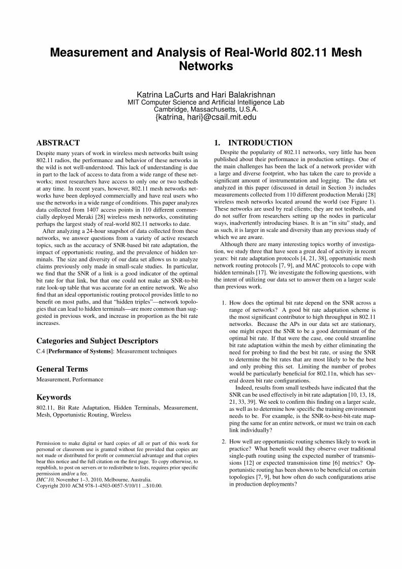
published about their performance in production settings. One ofthe main challenges has been the lack of a network provider witha large and diverse footprint, who has taken the care to provide asignificant amount of instrumentation and logging. The data setanalyzed in this paper (discussed in detail in Section 3) includesmeasurements collected from 110 different production Meraki [28]wireless mesh networks located around the world (see Figure 1).These networks are used by real clients; they are not testbeds, anddo not suffer from researchers setting up the nodes in particularways, inadvertently introducing biases. It is an “in situ” study, andas such, it is larger in scale and diversity than any previous study ofwhich we are aware.

Although there are many interesting topics worthy of investiga-tion, we study three that have seen a great deal of activity in recentyears: bit rate adaptation protocols [4, 21, 38], opportunistic meshnetwork routing protocols [7, 9], and MAC protocols to cope withhidden terminals [17]. We investigate the following questions, withthe intent of utilizing our data set to answer them on a larger scalethan previous work.

1. How does the optimal bit rate depend on the SNR across arange of networks? A good bit rate adaptation scheme isthe most significant contributor to high throughput in 802.11networks. Because the APs in our data set are stationary,one might expect the SNR to be a good determinant of theoptimal bit rate. If that were the case, one could streamlinebit rate adaptation within the mesh by either eliminating theneed for probing to find the best bit rate, or using the SNRto determine the bit rates that are most likely to be the bestand only probing this set. Limiting the number of probeswould be particularly beneficial for 802.11n, which has sev-eral dozen bit rate configurations.

Indeed, results from small testbeds have indicated that theSNR can be used effectively in bit rate adaptation [10, 13, 18,21, 33, 39]. We seek to confirm this finding on a larger scale,as well as to determine how specific the training environmentneeds to be. For example, is the SNR-to-best-bit-rate map-ping the same for an entire network, or must we train on eachlink individually?

2. How well are opportunistic routing schemes likely to work inpractice? What benefit would they observe over traditionalsingle-path routing using the expected number of transmis-sions [12] or expected transmission time [6] metrics? Op-portunistic routing has been shown to be beneficial on certaintopologies [7, 9], but how often do such configurations arisein production deployments?

Figure 1: Approximate locations of networks in our data set(some are co-located). This data set exhibits more geographicdiversity than any previous study of which we are aware.

3. How common are hidden triples—topologies that can lead tohidden terminals—in these diverse real-world deployments?Interference caused by hidden terminals can affect even anideal rate adaptation protocol, however previous studies havenot provided conclusive answers as to how frequently hiddenterminals occur. For instance, [11], [17], [23], [25], and [29],report proportions of hidden terminals ranging from 10% to50% in a particular testbed or network. The disagreementsamong these previous studies suggest that the prevalence ofhidden terminals depends heavily on the relative positions ofthe nodes and the peculiarities of each network. We mea-sure how much variation there is in the proportion of hiddentriples across different topologies and how it changes withthe transmit bit rate.

After analyzing a 24-hour snapshot of data from 1407 APs in110 networks, our main findings are as follows:

1. When trained on a particular link in a static setting, the SNRis a very good indicator of the optimal bit rate for 802.11b/gand a surprisingly good indicator for 802.11n, given the num-ber of bit rates present. For 802.11b/g networks, we find thatwhen trained on each link, the SNR can frequently predictthe best bit rate over 95% of the time. In 802.11n, we findthat a trained look-up table keyed by SNR, while not perfect,can substantially reduce the number of bit rates that need tobe probed. However, in both 802.11b/g and 802.11n, usingother links in the network to train provides little benefit, in-dicating that it would not be possible to build one SNR-to-bit-rate look-up table that worked well for an entire network.

2. Analyzing all networks with at least five access points, wefind that the expected number of transmissions incurred by anidealized opportunistic routing protocol (such as ExOR [7] orMORE [9] without overheads) would be rather small, evenif an almost-perfect bit rate adaptation algorithm were used:there is no improvement for at least 13% of node pairs, andthe median improvement is frequently less than 7%.

3. The prevalence of hidden triples—topologies where nodes Aand B cannot hear each other, but node C can hear both ofthem—depends on the bit rate. At the lowest bit rate of 1Mbit/s, and thresholding on a very low success probabilityof 10% (i.e., considering two nodes to be neighbors if theycan hear each other at least 10% of the time), we find that themedian number of hidden triples is over 13%. Hidden triplesoccur with far greater frequency at higher bit rates.

We also find that, as the bit rates increase, the probabilityof nodes hearing each other decreases. This result is hardly

surprising, but what is noteworthy is that there is a high vari-ance: the mean number of nodes that can hear each otherreduces, but the standard deviation is large. This variance im-plies that there are node pairs that are able to hear each otherat a higher bit rate but not at a lower one at around the sametime, most likely because of differences in modulation andcoding (e.g., spread spectrum vs. OFDM). As a result, onecannot always conclude that higher bit rates have poorer re-ception properties than lower ones under similar conditions.

The rest of this paper is organized as follows. After discussingrelated work in the next section, we describe the relevant featuresof our data set in Section 3. Section 4 analyzes the performance ofvarious bit rates and how it relates to SNR, Section 5 discusses theperformance of opportunistic routing vs. traditional routing, andSection 6 analyzes the frequency of hidden triples. We conclude inSection 7.

2. RELATED WORKWe break related work into four sections. First, we discuss gen-

eral wireless measurement studies. Then we address each of thetopics of our study—SNR-based bit rate adaptation, opportunisticrouting, and hidden terminals—in turn.

2.1 Wireless Measurement StudiesUnlike this paper, most previous measurement studies focus on

results from single testbeds in fairly specific locations, such as uni-versities or corporate campuses. For example, Jigsaw [11] studiesa campus network with 39 APs. Their focus is merging traces ofpacket-level data. As such, they are able to calculate packet-levelstatistics that we cannot, but must employ complicated mergingtechniques. [14], [15], and [37] also deal with packet-level char-acteristics, again for only one network.

Henderson and Kotz [19] study the use of a campus network withover 550 APs and 7000 users. They focus on what types of devicesare most prevalent on the network and the types of data being trans-ferred. Though they have a fairly large testbed, they cannot captureinter-network diversity. Other campus studies address questions oftraffic load [20, 34] and mobility [27, 35].

Other wireless measurement papers focus on single testbeds inmore diverse locations. Rodrig et al. measure wireless in a hotspotsetting [31]. They study overhead, retransmissions, and the dynam-ics of bit rate adaptation in 802.11b/g. [2] studies user behavior andnetwork performance in a conference setting, as does [22].

Though the aforementioned studies make important contribu-tions toward understanding the behavior of wireless networks, theyare all limited by the scope of their testbeds. It is not possible todetermine which characteristics of 802.11 are invariant across net-works with access to only one network. Our data set, however,gives us this capability.

2.2 SNR-based Bit Rate AdaptationMost bit rate adaptation algorithms can be divided into two

types: those that adapt based on loss rates from probes, and thosethat adapt based on a estimate of channel quality. In algorithmsin the first category, for example SampleRate [4], nodes send oc-casional probes at different bit rates, and switch to the rate thatprovides the highest throughput (throughput being a function ofthe loss rate and the bit rate). Algorithms in the second categorymeasure the channel quality in some way (e.g., by sampling theSNR), and react based on the results of this measurement. In gen-eral, poor channel quality results in decreasing the bit rate, and viceversa. Here we take a closer look at studies which use the SNR as

an estimate of channel quality in adaptation algorithms, as this isthe approach we examine in Section 4.

SGRA [39] uses estimates of the SNR on a link to calculatethresholds for each bit rate, which define the range of SNRs forwhich a particular bit rate will work well. The authors find thatthe SNR can overestimate channel quality in the presence of inter-ference. RBAR [21] uses the SNR to derive thresholds, similar toSGRA. Here, however, it is the SNR at the receiver that is used todetermine these thresholds. The receiver’s desired rate is commu-nicated via RTS/CTS packets. RBAR also depends on a theoreticalestimate of the BER to select a bit rate. Although using the SNRat the receiver is likely more accurate than using the SNR at thesender, this scheme incurs relatively high overhead. OAR [33] issimilar to RBAR in the way in which it uses the SNR, but it main-tains the temporal fairness of 802.11. Other threshold-based SNRschemes include [10], [13], and [18].

Though all of these schemes report positive results from SNR-based rate adaptation, they are all evaluated on research testbeds orin simulation. None of them have been validated on real networks,much less across networks. In Section 4, we evaluate the accuracyof SNR-based bit rate adaptation across many networks. We alsoattempt to quantify the losses that are seen when a sub-optimal bitrate is selected (a sub-optimal bit rate being one that was not thebest for a particular SNR).

Other studies have explored using the SNR for a predictor ina mobile setting [8, 24]. Because of the nature of our data, weare only able to make conclusive claims for static environments.Though we find that a per-link SNR works well in these cases, wemake no claims that this finding would hold in a mobile setting.

Finally, other studies examine using measures of channel qualityother than the SNR for adaptation algorithms, for instance [3], [16],and [30]. Though potentially more accurate, these measures can becomplicated or difficult to obtain. We focus our efforts in Section 4towards using the SNR, as we find that it is simple to determine andperforms well enough for our needs.

2.3 Opportunistic RoutingIn Section 5, we measure the possible improvements that could

be seen in our networks using opportunistic routing. Here, we pro-vide a brief summary of how opportunistic routing differs fromstandard routing. In particular, we focus on the opportunistic rout-ing protocol ExOR [7] and the contrasting shortest-path routing al-gorithms using ETX [12] and ETT [6].

The ETX of a path is the expected number of transmissions itwill take to send a packet along that path, based on the deliveryprobability of the forward and reverse paths. Unless all links areperfect, the ETX of a path will be higher than the number of hopsin the path, and it is possible for a path with a large number of hopsto have a smaller ETX metric than a path with fewer hops.

The ETT metric is similar to the ETX metric, except that it allowsfor varying bit rates. The ETT of a path is the expected amountof time it will take to send a packet along that path, based on thedelivery probability of the forward and reverse paths, as well as thebit rate chosen by each node along the path.

A potential shortcoming of this type of shortest-path routing inwireless networks is that it does not take into account the broadcastnature of wireless [7]. When the source sends a packet to the firsthop in the path, the packet may in fact reach the second hop sinceit was broadcasted. In this case, it is redundant to send the packetfrom the first hop to the second. Opportunistic routing exploits thisscenario.

ExOR [7], in particular, works as follows. The source nodebroadcasts a packet, and a subset of nodes between it and the desti-

nation receive it. These nodes coordinate amongst themselves, andthe node in that subset that is closest to the destination broadcaststhe packet. A subset of nodes receive that broadcast, and so on untilthe packet reaches its destination. Note that it is unlikely that shortpaths would see much improvement due to opportunistic routing, asthere are not as many hops in the path to skip. It is also important topoint out that the overhead required by ExOR to coordinate packetbroadcasts is not inherent to opportunistic routing. Indeed, thereare opportunistic routing protocols that operate without this typeof coordination [9]. In Section 5.4 we quantify the improvementsthat an ideal opportunistic routing protocol (one with no overhead)could incur over shortest-path routing via ETX or ETT.

2.4 Hidden TerminalsHidden terminals occur when two nodes, A and B, are within

range of a third node, C, but not within range of each other. Be-cause A and B cannot sense each other, they may send packets toC simultaneously, and those packets will collide. Different studiesfind different numbers of hidden terminals in practice: Zigzag [17]assumes that 10% of node pairs are part of hidden terminals, whileJigsaw [11] finds that up to 50% of nodes in their networks couldbe part of hidden terminals. Both of these studies, as well as oth-ers [23, 25, 29], only study hidden terminals in one network ortestbed. In Section 6, we examine how frequently hidden terminalscan occur across many networks, as well as how this frequencychanges with the transmit bit rate.

3. DATAOur data set contains anonymized measurements collected from

110 geographically disperse Meraki [28] networks. These networksinclude a total of 1407 APs, and range in size from three APs to 203APs, with a median of 7 and a mean of about 13. Of these networks,77 used only 802.11b/g radios, 31 used only 802.11n APs, and twocontained a mix of both kinds of radios. 802.11n traffic used the20MHz channel. 72 of these networks were indoor networks, 17were outdoor, and 21 included both indoor and outdoor nodes.1

All radios are made by Atheros, which makes it possible for us toconduct meaningful inter-network comparisons when dealing withthe SNR (the way in which the SNR is reported can vary acrossvendors; see Section 3.1.1). Our data is made up of measurementsfrom controlled probes sent periodically between APs in the meshat varying bit rates. Though these probes are controlled, they aresent while the network is being used by real users.

3.1 Probe DataThe probe data contains loss rates and SNRs from broadcast

probes sent by each AP every 40 seconds (this is the default re-porting rate used in Meraki networks [5]). These probes are verysimilar to those used in Roofnet [32] to calculate the ETX met-ric [12]. The loss rate between AP1 and AP2 at a particular bit rateb is calculated as the average of the loss rates of each probe sentat rate b between AP1 and AP2 over the past 800 seconds, an in-terval used to make bit rate adaptation decisions in the productionnetworks. We collect data from each node every 300 seconds; thereported loss rate data is for the past 800 seconds, so one shouldthink of the data as a sliding window of the inter-AP loss rate atdifferent bit rates.

We refer to each collection of inter-AP loss rates at a set of mea-sured bit rates as a probe set. Note that one probe set representsaggregate data from roughly 800/40 = 20 probes for each bit rate.

1We ignore these networks when classifying by environment.

We refer to the set of bit rates present in probe set P as Prates. Eachbit rate b in Prates is associated with a loss rate, bloss.

We use the loss rates and SNRs of these probes to measure theaccuracy of SNR-based bit rate adaptation algorithms in Section 4,to measure the potential improvements from opportunistic routingin Section 5, and to determine the frequency of hidden terminalsin Section 6. Before delving into these problems, we discuss twoproperties of our data set in more detail.

3.1.1 SNREach received probe has an SNR value associated with it, re-

ported by the Atheros chip and logged on the Meraki device. TheMadWiFi driver reports an “RSSI” quantity on each packet recep-tion. The 802.11 standard does not specify how this informationshould be calculated, so different chipsets and drivers behave dif-ferently. The behavior of MadWiFi on the Atheros chipset is well-documented on the MadWiFi web site2 and has been verified byvarious researchers (including us in the past). The MadWiFi docu-mentation describes the RSSI it reports as follows:

“In MadWiFi, the reported RSSI for each packet is ac-tually equivalent to the Signal-to-Noise Ratio (SNR)and hence we can use the terms interchangeably. Thisdoes not necessarily hold for other drivers though.This is because the RSSI reported by the MadWiFiHAL is a value in dB that specifies the difference be-tween the signal level and noise level for each packet.Hence the driver calculates a packet’s absolute signallevel by adding the RSSI to the absolute noise level.”

In this paper, we use the term SNR rather than RSSI because theformer is a precise term while the latter varies between vendors.

The SNR for a given probe set is not always the same becausewireless channel properties vary with time. As mentioned, eachprobe set contains data from about 20 probes per each bit rate,which are averaged to produce tuples of the form

〈Sender, Bit rate, Mean loss rate, Most recent SNR〉

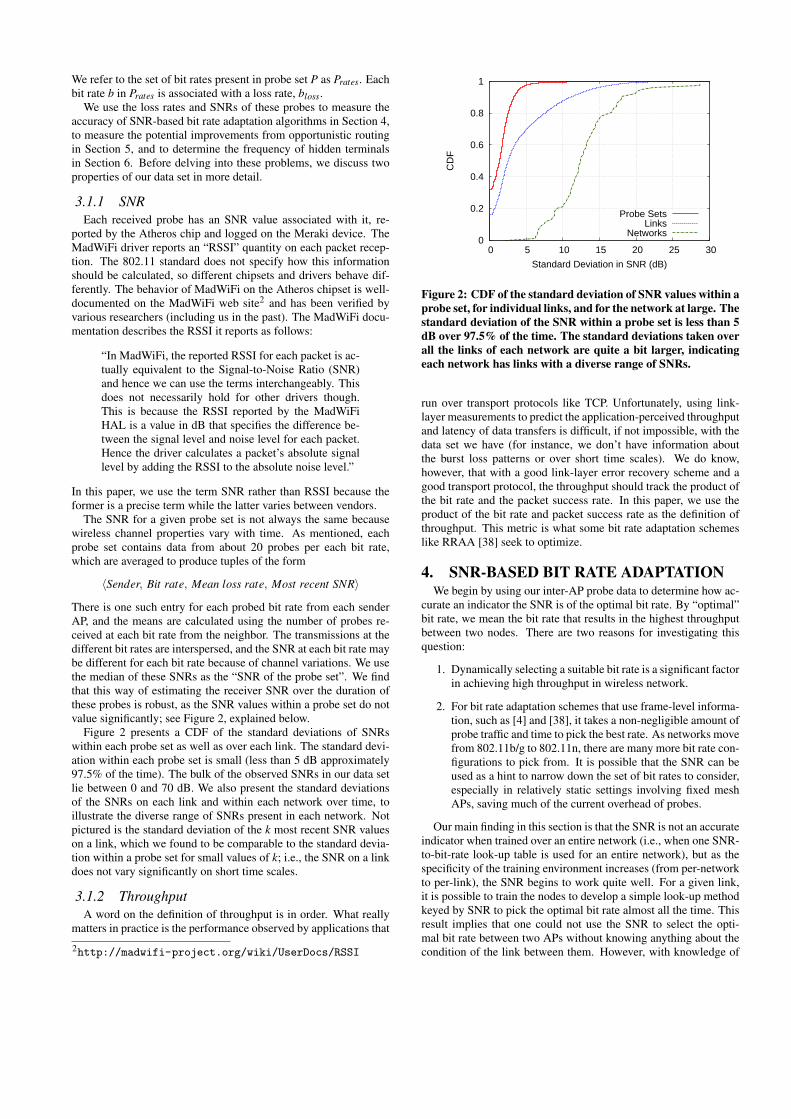
There is one such entry for each probed bit rate from each senderAP, and the means are calculated using the number of probes re-ceived at each bit rate from the neighbor. The transmissions at thedifferent bit rates are interspersed, and the SNR at each bit rate maybe different for each bit rate because of channel variations. We usethe median of these SNRs as the “SNR of the probe set”. We findthat this way of estimating the receiver SNR over the duration ofthese probes is robust, as the SNR values within a probe set do notvalue significantly; see Figure 2, explained below.

Figure 2 presents a CDF of the standard deviations of SNRswithin each probe set as well as over each link. The standard devi-ation within each probe set is small (less than 5 dB approximately97.5% of the time). The bulk of the observed SNRs in our data setlie between 0 and 70 dB. We also present the standard deviationsof the SNRs on each link and within each network over time, toillustrate the diverse range of SNRs present in each network. Notpictured is the standard deviation of the k most recent SNR valueson a link, which we found to be comparable to the standard devia-tion within a probe set for small values of k; i.e., the SNR on a linkdoes not vary significantly on short time scales.

3.1.2 ThroughputA word on the definition of throughput is in order. What really

matters in practice is the performance observed by applications that

2http://madwifi-project.org/wiki/UserDocs/RSSI

0

0.2

0.4

0.6

0.8

1

0 5 10 15 20 25 30

CD

F

Standard Deviation in SNR (dB)

Probe SetsLinks

Networks

Figure 2: CDF of the standard deviation of SNR values within aprobe set, for individual links, and for the network at large. Thestandard deviation of the SNR within a probe set is less than 5dB over 97.5% of the time. The standard deviations taken overall the links of each network are quite a bit larger, indicatingeach network has links with a diverse range of SNRs.

run over transport protocols like TCP. Unfortunately, using link-layer measurements to predict the application-perceived throughputand latency of data transfers is difficult, if not impossible, with thedata set we have (for instance, we don’t have information aboutthe burst loss patterns or over short time scales). We do know,however, that with a good link-layer error recovery scheme and agood transport protocol, the throughput should track the product ofthe bit rate and the packet success rate. In this paper, we use theproduct of the bit rate and packet success rate as the definition ofthroughput. This metric is what some bit rate adaptation schemeslike RRAA [38] seek to optimize.

4. SNR-BASED BIT RATE ADAPTATIONWe begin by using our inter-AP probe data to determine how ac-

curate an indicator the SNR is of the optimal bit rate. By “optimal”bit rate, we mean the bit rate that results in the highest throughputbetween two nodes. There are two reasons for investigating thisquestion:

1. Dynamically selecting a suitable bit rate is a significant factorin achieving high throughput in wireless network.

2. For bit rate adaptation schemes that use frame-level informa-tion, such as [4] and [38], it takes a non-negligible amount ofprobe traffic and time to pick the best rate. As networks movefrom 802.11b/g to 802.11n, there are many more bit rate con-figurations to pick from. It is possible that the SNR can beused as a hint to narrow down the set of bit rates to consider,especially in relatively static settings involving fixed meshAPs, saving much of the current overhead of probes.

Our main finding in this section is that the SNR is not an accurateindicator when trained over an entire network (i.e., when one SNR-to-bit-rate look-up table is used for an entire network), but as thespecificity of the training environment increases (from per-networkto per-link), the SNR begins to work quite well. For a given link,it is possible to train the nodes to develop a simple look-up methodkeyed by SNR to pick the optimal bit rate almost all the time. Thisresult implies that one could not use the SNR to select the opti-mal bit rate between two APs without knowing anything about thecondition of the link between them. However, with knowledge of

a link’s condition, a simple bit rate selection algorithm using theSNR would likely work very well. The caveat is that this resultholds in our data set for inter-AP communication. It is probablethat it would hold for static clients, but not as likely to hold formobile ones (see Section 4.6).

4.1 Bit Rate Selection Using SNRRecall that the SNR is a measure of how much a signal has been

corrupted by noise. Intuitively, a higher SNR indicates a “better”link, and one would expect to be able to send more information, i.e.,use a higher bit rate on that link. Similarly, a low SNR indicates apoor link, and one would expect to need a lower bit rate. It is thisintuition that motivates SNR-based bit rate adaptation. Indeed, thethroughput and optimal bit rate clearly depend on the SNR accord-ing to Shannon’s theorem, but the question is whether our relativelycoarsely-sampled SNR can be used as an accurate hint for deter-mining the correct bit rate. Our bit rate adaptation algorithm worksas follows: To select the bit rate for a link between AP1 and AP2,measure the SNR s on this link. Then, using a look-up table thatmaps SNR values to bit rates, look up s and use the correspondingbit rate.

The key question in this method is how to create the look-uptable from SNR to bit rate. For a probe set between AP1 and AP2,we define Popt as the bit rate that maximized the throughput for aparticular probe set, i.e.,

Popt = max{b× (1−bloss) : b ∈ Prates}

Given the SNR and Popt values from every probe set P in our dataset, we consider three options for creating the look-up table:

1. Network: For each network n and each SNR s representedin our data for n, assign bit rate b to s, where b is the mostfrequent value of Popt for SNR s (i.e., the bit rate that wasmost frequently the optimal bit rate for the probe sets withSNR s). For links in network n, select the bit rates by usingn’s look-up table.

2. AP: Instead of creating one look-up table per network, createone per AP. For a particular link, the source will use its ownlook-up table to select the bit rate, but this table will not varywith the destination.

3. Link: Instead of creating one look-up table per AP, createone per link. Use a link’s own table to select its bit rates.This approach differs from the AP approach in that each APnow has one table per neighbor.

As listed, each of these methods uses a more specific environ-ment than the last. As a result, each would have a different start-upcost. With the first, training needs to be done on the network as awhole, but not per-link. If one were to add a link to the network, thesame look-up table could still be used (though it may be beneficialto re-train if the network changed drastically). With the second,training would need to occur when a new node was added, but onlyat that node. With the third, training would need to occur everytime a new link was added, at both the source and destination ofthe link; this is discussed more in Section 4.5.

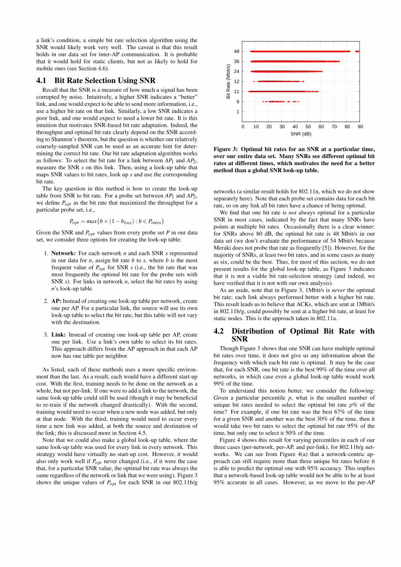
Note that we could also make a global look-up table, where thesame look-up table was used for every link in every network. Thisstrategy would have virtually no start-up cost. However, it wouldalso only work well if Popt never changed (i.e., if it were the casethat, for a particular SNR value, the optimal bit rate was always thesame regardless of the network or link that we were using). Figure 3shows the unique values of Popt for each SNR in our 802.11b/g

1

6

11

12

24

36

48

0 10 20 30 40 50 60 70 80 90

Bit

Rat

e (M

bit/s

)

SNR (dB)

Figure 3: Optimal bit rates for an SNR at a particular time,over our entire data set. Many SNRs see different optimal bitrates at different times, which motivates the need for a bettermethod than a global SNR look-up table.

networks (a similar result holds for 802.11n, which we do not showseparately here). Note that each probe set contains data for each bitrate, so on any link all bit rates have a chance of being optimal.

We find that one bit rate is not always optimal for a particularSNR in most cases, indicated by the fact that many SNRs havepoints at multiple bit rates. Occasionally there is a clear winner:for SNRs above 80 dB, the optimal bit rate is 48 Mbit/s in ourdata set (we don’t evaluate the performance of 54 Mbit/s becauseMeraki does not probe that rate as frequently [5]). However, for themajority of SNRs, at least two bit rates, and in some cases as manyas six, could be the best. Thus, for most of this section, we do notpresent results for the global look-up table, as Figure 3 indicatesthat it is not a viable bit rate-selection strategy (and indeed, wehave verified that it is not with our own analysis).

As an aside, note that in Figure 3, 1Mbit/s is never the optimalbit rate; each link always performed better with a higher bit rate.This result leads us to believe that ACKs, which are sent at 1Mbit/sin 802.11b/g, could possibly be sent at a higher bit rate, at least forstatic nodes. This is the approach taken in 802.11a.

4.2 Distribution of Optimal Bit Rate withSNR

Though Figure 3 shows that one SNR can have multiple optimalbit rates over time, it does not give us any information about thefrequency with which each bit rate is optimal. It may be the casethat, for each SNR, one bit rate is the best 99% of the time over allnetworks, in which case even a global look-up table would work99% of the time.

To understand this notion better, we consider the following:Given a particular percentile p, what is the smallest number ofunique bit rates needed to select the optimal bit rate p% of thetime? For example, if one bit rate was the best 67% of the timefor a given SNR and another was the best 30% of the time, then itwould take two bit rates to select the optimal bit rate 95% of thetime, but only one to select it 50% of the time.

Figure 4 shows this result for varying percentiles in each of ourthree cases (per-network, per-AP, and per-link), for 802.11b/g net-works. We can see from Figure 4(a) that a network-centric ap-proach can still require more than three unique bit rates before itis able to predict the optimal one with 95% accuracy. This impliesthat a network-based look-up table would not be able to be at least95% accurate in all cases. However, as we move to the per-AP

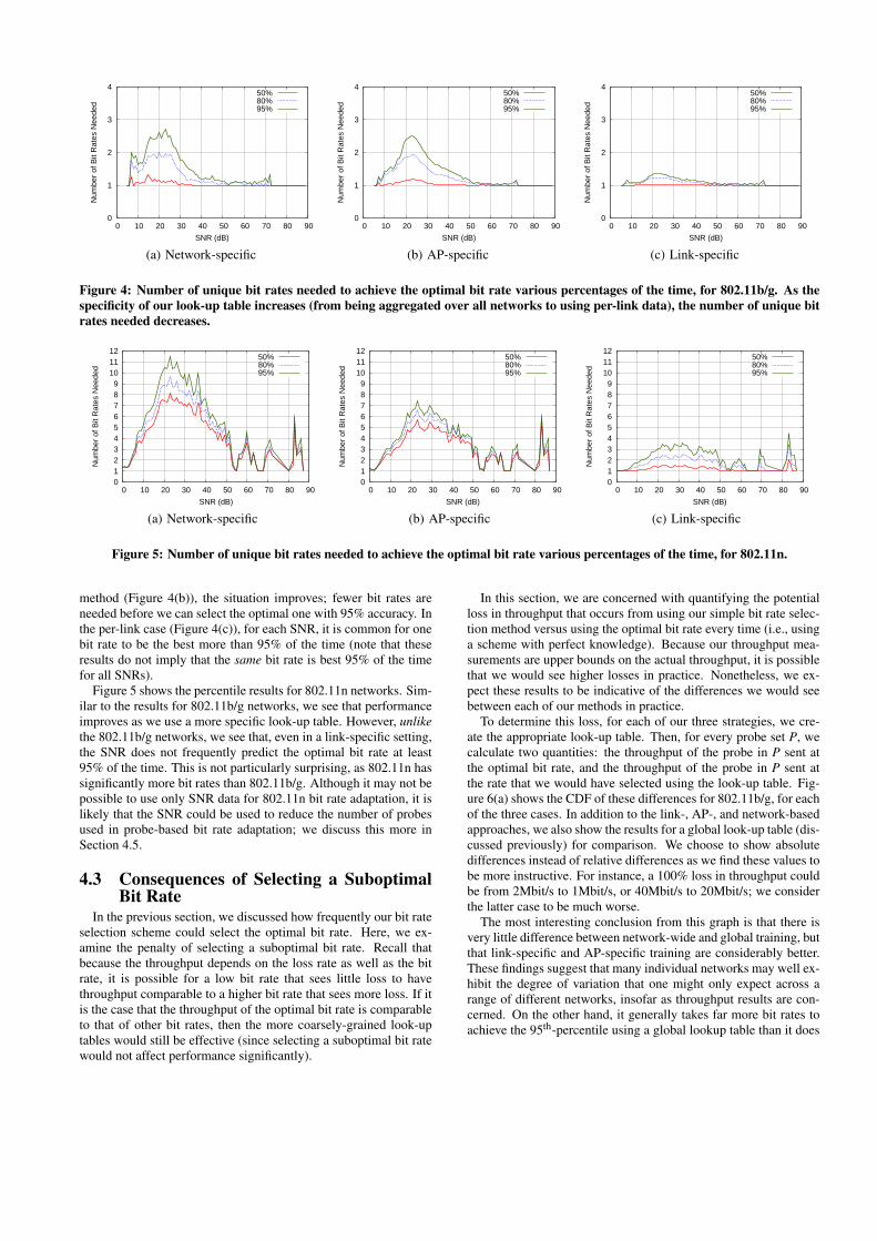
0

1

2

3

4

0 10 20 30 40 50 60 70 80 90

Num

ber

of B

it R

ates

Nee

ded

SNR (dB)

50%80%95%

(a) Network-specific

0

1

2

3

4

0 10 20 30 40 50 60 70 80 90

Num

ber

of B

it R

ates

Nee

ded

SNR (dB)

50%80%95%

(b) AP-specific

0

1

2

3

4

0 10 20 30 40 50 60 70 80 90

Num

ber

of B

it R

ates

Nee

ded

SNR (dB)

50%80%95%

(c) Link-specific

Figure 4: Number of unique bit rates needed to achieve the optimal bit rate various percentages of the time, for 802.11b/g. As thespecificity of our look-up table increases (from being aggregated over all networks to using per-link data), the number of unique bitrates needed decreases.

0 1 2 3 4 5 6 7 8 9

10 11 12

0 10 20 30 40 50 60 70 80 90

Num

ber

of B

it R

ates

Nee

ded

SNR (dB)

50%80%95%

(a) Network-specific

0 1 2 3 4 5 6 7 8 9

10 11 12

0 10 20 30 40 50 60 70 80 90

Num

ber

of B

it R

ates

Nee

ded

SNR (dB)

50%80%95%

(b) AP-specific

0 1 2 3 4 5 6 7 8 9

10 11 12

0 10 20 30 40 50 60 70 80 90

Num

ber

of B

it R

ates

Nee

ded

SNR (dB)

50%80%95%

(c) Link-specific

Figure 5: Number of unique bit rates needed to achieve the optimal bit rate various percentages of the time, for 802.11n.

method (Figure 4(b)), the situation improves; fewer bit rates areneeded before we can select the optimal one with 95% accuracy. Inthe per-link case (Figure 4(c)), for each SNR, it is common for onebit rate to be the best more than 95% of the time (note that theseresults do not imply that the same bit rate is best 95% of the timefor all SNRs).

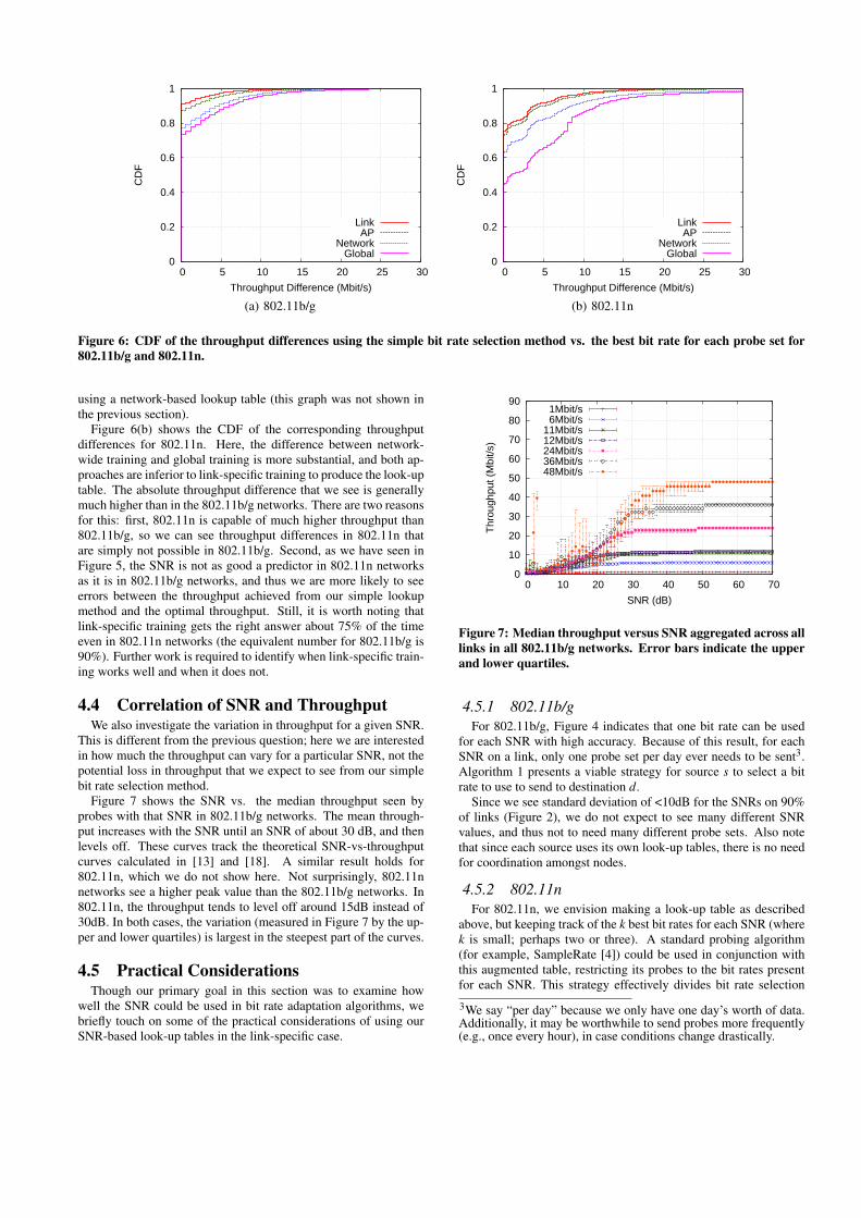
Figure 5 shows the percentile results for 802.11n networks. Sim-ilar to the results for 802.11b/g networks, we see that performanceimproves as we use a more specific look-up table. However, unlikethe 802.11b/g networks, we see that, even in a link-specific setting,the SNR does not frequently predict the optimal bit rate at least95% of the time. This is not particularly surprising, as 802.11n hassignificantly more bit rates than 802.11b/g. Although it may not bepossible to use only SNR data for 802.11n bit rate adaptation, it islikely that the SNR could be used to reduce the number of probesused in probe-based bit rate adaptation; we discuss this more inSection 4.5.

4.3 Consequences of Selecting a SuboptimalBit Rate

In the previous section, we discussed how frequently our bit rateselection scheme could select the optimal bit rate. Here, we ex-amine the penalty of selecting a suboptimal bit rate. Recall thatbecause the throughput depends on the loss rate as well as the bitrate, it is possible for a low bit rate that sees little loss to havethroughput comparable to a higher bit rate that sees more loss. If itis the case that the throughput of the optimal bit rate is comparableto that of other bit rates, then the more coarsely-grained look-uptables would still be effective (since selecting a suboptimal bit ratewould not affect performance significantly).

In this section, we are concerned with quantifying the potentialloss in throughput that occurs from using our simple bit rate selec-tion method versus using the optimal bit rate every time (i.e., usinga scheme with perfect knowledge). Because our throughput mea-surements are upper bounds on the actual throughput, it is possiblethat we would see higher losses in practice. Nonetheless, we ex-pect these results to be indicative of the differences we would seebetween each of our methods in practice.

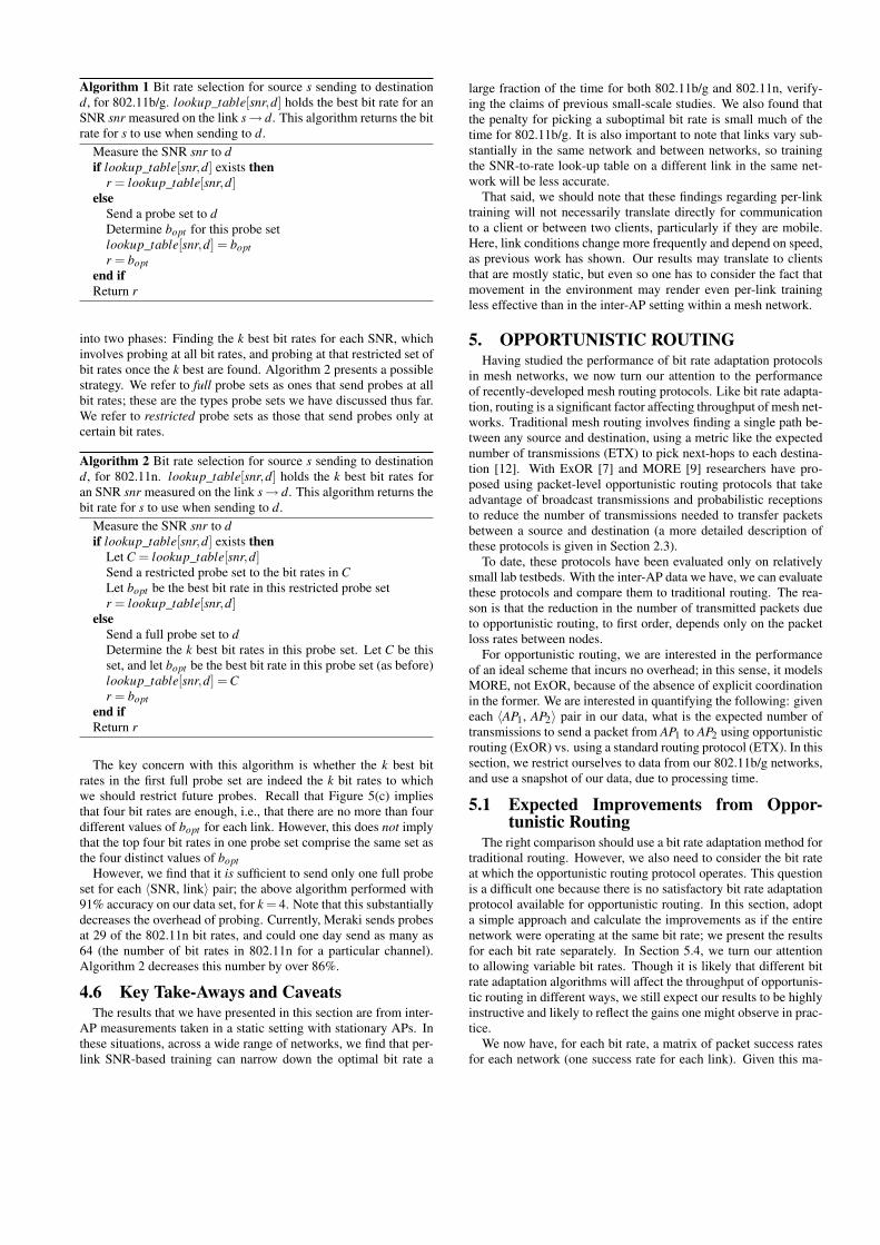
To determine this loss, for each of our three strategies, we cre-ate the appropriate look-up table. Then, for every probe set P, wecalculate two quantities: the throughput of the probe in P sent atthe optimal bit rate, and the throughput of the probe in P sent atthe rate that we would have selected using the look-up table. Fig-ure 6(a) shows the CDF of these differences for 802.11b/g, for eachof the three cases. In addition to the link-, AP-, and network-basedapproaches, we also show the results for a global look-up table (dis-cussed previously) for comparison. We choose to show absolutedifferences instead of relative differences as we find these values tobe more instructive. For instance, a 100% loss in throughput couldbe from 2Mbit/s to 1Mbit/s, or 40Mbit/s to 20Mbit/s; we considerthe latter case to be much worse.

The most interesting conclusion from this graph is that there isvery little difference between network-wide and global training, butthat link-specific and AP-specific training are considerably better.These findings suggest that many individual networks may well ex-hibit the degree of variation that one might only expect across arange of different networks, insofar as throughput results are con-cerned. On the other hand, it generally takes far more bit rates toachieve the 95th-percentile using a global lookup table than it does

0

0.2

0.4

0.6

0.8

1

0 5 10 15 20 25 30

CD

F

Throughput Difference (Mbit/s)

LinkAP

NetworkGlobal

(a) 802.11b/g

0

0.2

0.4

0.6

0.8

1

0 5 10 15 20 25 30

CD

F

Throughput Difference (Mbit/s)

LinkAP

NetworkGlobal

(b) 802.11n

Figure 6: CDF of the throughput differences using the simple bit rate selection method vs. the best bit rate for each probe set for802.11b/g and 802.11n.

using a network-based lookup table (this graph was not shown inthe previous section).

Figure 6(b) shows the CDF of the corresponding throughputdifferences for 802.11n. Here, the difference between network-wide training and global training is more substantial, and both ap-proaches are inferior to link-specific training to produce the look-uptable. The absolute throughput difference that we see is generallymuch higher than in the 802.11b/g networks. There are two reasonsfor this: first, 802.11n is capable of much higher throughput than802.11b/g, so we can see throughput differences in 802.11n thatare simply not possible in 802.11b/g. Second, as we have seen inFigure 5, the SNR is not as good a predictor in 802.11n networksas it is in 802.11b/g networks, and thus we are more likely to seeerrors between the throughput achieved from our simple lookupmethod and the optimal throughput. Still, it is worth noting thatlink-specific training gets the right answer about 75% of the timeeven in 802.11n networks (the equivalent number for 802.11b/g is90%). Further work is required to identify when link-specific train-ing works well and when it does not.

4.4 Correlation of SNR and ThroughputWe also investigate the variation in throughput for a given SNR.

This is different from the previous question; here we are interestedin how much the throughput can vary for a particular SNR, not thepotential loss in throughput that we expect to see from our simplebit rate selection method.

Figure 7 shows the SNR vs. the median throughput seen byprobes with that SNR in 802.11b/g networks. The mean through-put increases with the SNR until an SNR of about 30 dB, and thenlevels off. These curves track the theoretical SNR-vs-throughputcurves calculated in [13] and [18]. A similar result holds for802.11n, which we do not show here. Not surprisingly, 802.11nnetworks see a higher peak value than the 802.11b/g networks. In802.11n, the throughput tends to level off around 15dB instead of30dB. In both cases, the variation (measured in Figure 7 by the up-per and lower quartiles) is largest in the steepest part of the curves.

4.5 Practical ConsiderationsThough our primary goal in this section was to examine how

well the SNR could be used in bit rate adaptation algorithms, webriefly touch on some of the practical considerations of using ourSNR-based look-up tables in the link-specific case.

0

10

20

30

40

50

60

70

80

90

0 10 20 30 40 50 60 70

Thr

ough

put (

Mbi

t/s)

SNR (dB)

1Mbit/s6Mbit/s

11Mbit/s12Mbit/s24Mbit/s36Mbit/s48Mbit/s

Figure 7: Median throughput versus SNR aggregated across alllinks in all 802.11b/g networks. Error bars indicate the upperand lower quartiles.

4.5.1 802.11b/gFor 802.11b/g, Figure 4 indicates that one bit rate can be used

for each SNR with high accuracy. Because of this result, for eachSNR on a link, only one probe set per day ever needs to be sent3.Algorithm 1 presents a viable strategy for source s to select a bitrate to use to send to destination d.

Since we see standard deviation of <10dB for the SNRs on 90%of links (Figure 2), we do not expect to see many different SNRvalues, and thus not to need many different probe sets. Also notethat since each source uses its own look-up tables, there is no needfor coordination amongst nodes.

4.5.2 802.11nFor 802.11n, we envision making a look-up table as described

above, but keeping track of the k best bit rates for each SNR (wherek is small; perhaps two or three). A standard probing algorithm(for example, SampleRate [4]) could be used in conjunction withthis augmented table, restricting its probes to the bit rates presentfor each SNR. This strategy effectively divides bit rate selection

3We say “per day” because we only have one day’s worth of data.Additionally, it may be worthwhile to send probes more frequently(e.g., once every hour), in case conditions change drastically.

Algorithm 1 Bit rate selection for source s sending to destinationd, for 802.11b/g. lookup_table[snr,d] holds the best bit rate for anSNR snr measured on the link s→ d. This algorithm returns the bitrate for s to use when sending to d.

Measure the SNR snr to dif lookup_table[snr,d] exists then

r = lookup_table[snr,d]else

Send a probe set to dDetermine bopt for this probe setlookup_table[snr,d] = boptr = bopt

end ifReturn r

into two phases: Finding the k best bit rates for each SNR, whichinvolves probing at all bit rates, and probing at that restricted set ofbit rates once the k best are found. Algorithm 2 presents a possiblestrategy. We refer to full probe sets as ones that send probes at allbit rates; these are the types probe sets we have discussed thus far.We refer to restricted probe sets as those that send probes only atcertain bit rates.

Algorithm 2 Bit rate selection for source s sending to destinationd, for 802.11n. lookup_table[snr,d] holds the k best bit rates foran SNR snr measured on the link s → d. This algorithm returns thebit rate for s to use when sending to d.

Measure the SNR snr to dif lookup_table[snr,d] exists then

Let C = lookup_table[snr,d]Send a restricted probe set to the bit rates in CLet bopt be the best bit rate in this restricted probe setr = lookup_table[snr,d]

elseSend a full probe set to dDetermine the k best bit rates in this probe set. Let C be thisset, and let bopt be the best bit rate in this probe set (as before)lookup_table[snr,d] = Cr = bopt

end ifReturn r

The key concern with this algorithm is whether the k best bitrates in the first full probe set are indeed the k bit rates to whichwe should restrict future probes. Recall that Figure 5(c) impliesthat four bit rates are enough, i.e., that there are no more than fourdifferent values of bopt for each link. However, this does not implythat the top four bit rates in one probe set comprise the same set asthe four distinct values of bopt

However, we find that it is sufficient to send only one full probeset for each 〈SNR, link〉 pair; the above algorithm performed with91% accuracy on our data set, for k = 4. Note that this substantiallydecreases the overhead of probing. Currently, Meraki sends probesat 29 of the 802.11n bit rates, and could one day send as many as64 (the number of bit rates in 802.11n for a particular channel).Algorithm 2 decreases this number by over 86%.

4.6 Key Take-Aways and CaveatsThe results that we have presented in this section are from inter-

AP measurements taken in a static setting with stationary APs. Inthese situations, across a wide range of networks, we find that per-link SNR-based training can narrow down the optimal bit rate a

large fraction of the time for both 802.11b/g and 802.11n, verify-ing the claims of previous small-scale studies. We also found thatthe penalty for picking a suboptimal bit rate is small much of thetime for 802.11b/g. It is also important to note that links vary sub-stantially in the same network and between networks, so trainingthe SNR-to-rate look-up table on a different link in the same net-work will be less accurate.

That said, we should note that these findings regarding per-linktraining will not necessarily translate directly for communicationto a client or between two clients, particularly if they are mobile.Here, link conditions change more frequently and depend on speed,as previous work has shown. Our results may translate to clientsthat are mostly static, but even so one has to consider the fact thatmovement in the environment may render even per-link trainingless effective than in the inter-AP setting within a mesh network.

5. OPPORTUNISTIC ROUTINGHaving studied the performance of bit rate adaptation protocols

in mesh networks, we now turn our attention to the performanceof recently-developed mesh routing protocols. Like bit rate adapta-tion, routing is a significant factor affecting throughput of mesh net-works. Traditional mesh routing involves finding a single path be-tween any source and destination, using a metric like the expectednumber of transmissions (ETX) to pick next-hops to each destina-tion [12]. With ExOR [7] and MORE [9] researchers have pro-posed using packet-level opportunistic routing protocols that takeadvantage of broadcast transmissions and probabilistic receptionsto reduce the number of transmissions needed to transfer packetsbetween a source and destination (a more detailed description ofthese protocols is given in Section 2.3).

To date, these protocols have been evaluated only on relativelysmall lab testbeds. With the inter-AP data we have, we can evaluatethese protocols and compare them to traditional routing. The rea-son is that the reduction in the number of transmitted packets dueto opportunistic routing, to first order, depends only on the packetloss rates between nodes.

For opportunistic routing, we are interested in the performanceof an ideal scheme that incurs no overhead; in this sense, it modelsMORE, not ExOR, because of the absence of explicit coordinationin the former. We are interested in quantifying the following: giveneach 〈AP1, AP2〉 pair in our data, what is the expected number oftransmissions to send a packet from AP1 to AP2 using opportunisticrouting (ExOR) vs. using a standard routing protocol (ETX). In thissection, we restrict ourselves to data from our 802.11b/g networks,and use a snapshot of our data, due to processing time.

5.1 Expected Improvements from Oppor-tunistic Routing

The right comparison should use a bit rate adaptation method fortraditional routing. However, we also need to consider the bit rateat which the opportunistic routing protocol operates. This questionis a difficult one because there is no satisfactory bit rate adaptationprotocol available for opportunistic routing. In this section, adopta simple approach and calculate the improvements as if the entirenetwork were operating at the same bit rate; we present the resultsfor each bit rate separately. In Section 5.4, we turn our attentionto allowing variable bit rates. Though it is likely that different bitrate adaptation algorithms will affect the throughput of opportunis-tic routing in different ways, we still expect our results to be highlyinstructive and likely to reflect the gains one might observe in prac-tice.

We now have, for each bit rate, a matrix of packet success ratesfor each network (one success rate for each link). Given this ma-

0

0.2

0.4

0.6

0.8

1

0 0.2 0.4 0.6 0.8 1

CD

F

Fraction Improvement of ExOR over ETX

1 Mbit/s6 Mbit/s

11 Mbit/s12 Mbit/s24 Mbit/s36 Mbit/s48 Mbit/s

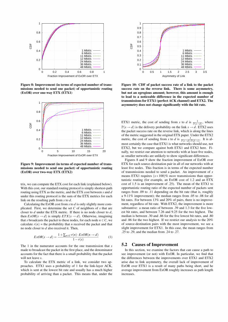
Figure 8: Improvement (in terms of expected number of trans-missions needed to send one packet) of opportunistic routing(ExOR) over one-way ETX (ETX1)

0

0.2

0.4

0.6

0.8

1

0 5 10 15 20

CD

F

Fraction Improvement of ExOR over ETX

1 Mbit/s6 Mbit/s

11 Mbit/s12 Mbit/s24 Mbit/s36 Mbit/s48 Mbit/s

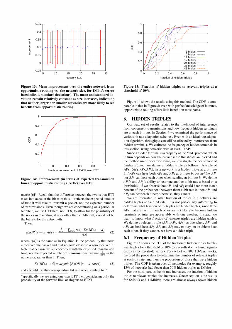
Figure 9: Improvement (in terms of expected number of trans-missions needed to send one packet) of opportunistic routing(ExOR) over two-way ETX (ETX2)

trix, we can compute the ETX cost for each link (explained below).With this cost, our standard routing protocol is simply shortest-pathrouting using ETX as the metric, and the ETX cost between s and dunder this routing protocol is the sum of the ETX metrics for eachlink on the resulting path from s to d.

Calculating the ExOR cost from s to d is only slightly more com-plicated. First, we determine the set C of neighbors of s that arecloser to d under the ETX metric. If there is no node closer to d,then ExOR(s → d) is simply ET X(s → d). Otherwise, imaginingthat s broadcasts the packet to these nodes, for each node n ∈C, wecalculate r(n) = the probability that n received the packet and thatno node closer to d also received it. Then,

ExOR(s → d) =1+∑n∈C r(n) ·ExOR(n → d)

1− r(s)(1)

The 1 in the numerator accounts for the one transmission that smade to broadcast the packet in the first place, and the denominatoraccounts for the fact that there is a small probability that the packetwill not leave s.

To calculate the ETX metric of a link, we consider two ap-proaches. ETX1 uses a probability of 1 for the link-layer ACK,which is sent at the lowest bit rate and usually has a much higherprobability of arriving than a packet. This means that, under the

0

0.1

0.2

0.3

0.4

0.5

0.6

0.7

0.8

0.9

1

0 0.5 1 1.5 2 2.5 3 3.5

CD

F

Asymmetry of Link

1 Mbit/s6 Mbit/s

11 Mbit/s12 Mbit/s24 Mbit/s36 Mbit/s48 Mbit/s

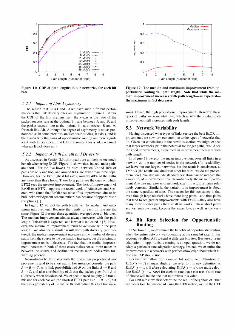
Figure 10: CDF of packet success rate of a link to the packetsuccess rate on the reverse link. There is some asymmetry,but not an egregious amount; however, this amount is enoughto lead to a noticeable difference in the expected number oftransmissions for ETX1 (perfect ACK channel) and ETX2. Theasymmetry does not change significantly with the bit rate.

ETX1 metric, the cost of sending from s to d is 1P(s→d) , where

P(s → d) is the delivery probability on the link s → d. ETX2 usesthe packet success rate on the reverse link, which is along the linesof the metric suggested in the original ETX paper. Under the ETX2metric, the cost of sending from s to d is 1

P(s→d)·P(d→s) . It is al-most certainly the case that ETX1 is what networks should use, notETX2, but we compare against both ETX1 and ETX2 here. Fi-nally, we restrict our attention to networks with at least five nodes,as smaller networks are unlikely to show significant differences.

Figures 8 and 9 show the fraction improvement of ExOR overETX for each source-destination pair in all of our networks with atleast five nodes. This fraction is in terms of the expected numberof transmissions needed to send a packet. An improvement of xmeans ETX1 requires (x ∗ 100)% more transmissions than oppor-tunistic routing (for example, an ExOR cost of 1.2 and an ETXcost of 1.5 is an improvement of .25). The mean of the ETX1 toopportunistic routing ratio of the expected number of packets sentranges from .09 to .11 depending on the bit rate (that is, roughlya 9-11% improvement); the median ranges from .05 to .08 for allbit rates. For between 13% and 20% of pairs, there is no improve-ment, regardless of bit rate. With ETX2, the improvement is moresubstantive: a mean ratio of between .39 and 1.3 for the five low-est bit rates, and between 7.26 and 9.25 for the two highest. Themedian is between .30 and .86 for the five lowest bit rates, and .80and .86 for the two highest. If we restrict our analysis to the 20%of source-destination pairs with the most improvement, we see aslight improvement for ETX1. In this case, the mean ranges from.25 to .29, and the median from .24 to .27.

5.2 Causes of ImprovementIn this section, we examine the factors that can cause a path to

see improvement (or not) with ExOR. In particular, we find thatthe differences between the improvements over ETX1 and ETX2arise due to link asymmetry, the overall lack of improvement ofExOR over ETX1 is a result of many paths being short, and heaverage improvement from ExOR roughly increases as path lengthincreases.

0

0.2

0.4

0.6

0.8

1

1 2 3 4 5 6 7 8 9

CD

F

Path Length (Number of Hops)

1 Mbit/s6 Mbit/s

11 Mbit/s12 Mbit/s24 Mbit/s36 Mbit/s48 Mbit/s

Figure 11: CDF of path lengths in our networks, for each bitrate.

5.2.1 Impact of Link AsymmetryThe reason that ETX1 and ETX2 have such different perfor-

mance is that link delivery rates are asymmetric. Figure 10 showsthe CDF of the link asymmetries: the x-axis is the ratio of thepacket success rate at the optimal bit rate between A and B, andthe packet success rate at the optimal bit rate between B and A,for each link AB. Although the degree of asymmetry is not as pro-nounced as in some previous smaller-scale studies, it exists, and isthe reason why the gains of opportunistic routing are more signif-icant with ETX2 (recall that ETX2 assumes a lossy ACK-channelwhereas ETX1 does not).

5.2.2 Impact of Path Length and DiversityAs discussed in Section 2.3, short paths are unlikely to see much

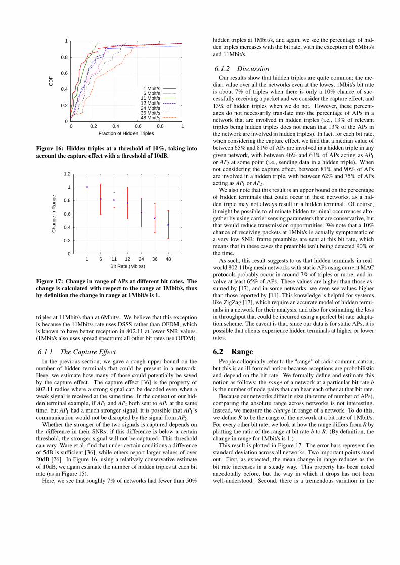
benefit when using ExOR. Figure 11 shows that, indeed, most pathsare short. For the five lowest bit rates, between 30 and 40% ofpaths are only one hop, and around 80% are fewer than three hops.However, for the two highest bit rates, roughly 40% of the pathsare more than three hops. These long paths are the ones on whichETX2 sees the greatest improvement. The lack of improvement ofExOR over ETX1 supports the recent work of Afanasyev and Sno-eren, who found that ExOR sees most of its improvement due to itsbulk-acknowledgment scheme rather than because of opportunisticreceptions [1].

In Figure 12 we plot the path length vs. the median and max-imum improvement. Because the trends for each bit rate are thesame, Figure 12 presents these quantities averaged over all bit rates.The median improvement almost always increases with the pathlength. This result is expected, and is what is indicated in [7]. How-ever, the maximum improvement tends to decrease with the pathlength. We also see a similar result with path diversity (not pic-tured): the median improvement increases as the number of diversepaths from the source to the destination increases, but the maximumimprovement tends to decrease. The fact that the median improve-ment increases in both of these cases makes sense; more nodes inbetween the source and destination means more nodes with for-warding potential.

Non-intuitively, the paths with the maximum proportional im-provements tend to be short paths. For instance, consider the pathA → B → C, with link probabilities of .9 on the links A → B andB →C, and also a probability of .3 that the packet goes from A toC directly when broadcasted. We expect to need roughly 2.2 trans-mission for each packet (the shortest ETX1 path is A → B →C, butthere is a probability of .3 that ExOR will reduce this to 1 transmis-

0

0.2

0.4

0.6

0.8

1

1 2 3 4 5 6 7 8

Impr

ovem

ent

Path Length (Number of Hops)

MedianMaximum

Figure 12: The median and maximum improvement from op-portunistic routing vs. path length. Note that while the me-dian improvement increases with path length—as expected—the maximum in fact decreases.

sion). Hence, the high proportional improvement. However, thesetypes of paths are somewhat rare, which is why the median pathimprovement still increases with path length.

5.3 Network VariabilityHaving discussed what types of links see see the best ExOR im-

provements, we now turn our attention to the types of networks thatdo. Given our conclusions in the previous section, we might expectthat larger networks (with the potential for longer paths) would seethe good improvements, as the median improvement increases withpath length.

In Figure 13 we plot the mean improvement over all links in anetwork vs. the number of nodes in the network (for readability,we leave out our largest networks, but the result is consistent), at1Mbit/s (the results are similar at other bit rates; we do not presentthem here). We also include standard deviation bars to indicate thevariability of improvement. Counter-intuitively, the mean improve-ment does not increase with network size; in fact, it remains rela-tively constant. Similarly, the variability in improvement is aboutthe same regardless of size. The reason for this constancy is thateven though large networks have more long paths—and thus pathsthat tend to see greater improvements with ExOR—they also havemany more shorter paths than small networks. These short pathssee less improvement, keeping the mean low, as well as the vari-ance.

5.4 Bit Rate Selection for OpportunisticRouting

In Section 5.1, we examined the benefits of opportunistic routingwhen the entire network was operating at the same bit rate. In thissection, we allow APs to send at different bit rates. Because bit rateadaptation in opportunistic routing is an open question, we do notadapt a particular rate adaptation strategy. Instead, we examine theimprovements in a network with perfect knowledge about which bitrate each AP should use.

Because we allow for variable bit rates, our definition ofExOR(s → d) changes slightly; we refer to this new definition asExOR′(s → d). Before calculating ExOR(s → d), we must calcu-late ExOR′(s → d,rate) for each bit rate that s can use. s’s bit rateof choice will be the one that minimizes this value.

For a bit rate r, we first determine the set C of neighbors of s thatare closer to d, but instead of using the ETX metric, we use the ETT

-0.05

0

0.05

0.1

0.15

0.2

0.25

5 10 15 20 25 30

Impr

ovem

ent

Network Size

Figure 13: Mean improvement over the entire network fromopportunistic routing vs. the network size, for 1Mbit/s (errorbars indicate standard deviations). The mean and standard de-viation remain relatively constant as size increases, indicatingthat neither larger nor smaller networks are more likely to seebenefits from opportunistic routing.

0

0.2

0.4

0.6

0.8

1

0 0.2 0.4 0.6 0.8 1

CD

F

Fraction Improvement of ExOR over ETT

Figure 14: Improvement (in terms of expected transmissiontime) of opportunistic routing (ExOR) over ETT.

metric [6]4. Recall that the difference between the two is that ETTtakes into account the bit rate; thus, it reflects the expected amountof time it will take to transmit a packet, not the expected numberof transmissions. Even though we are concentrating on a particularbit rate r, we use ETT here, not ETX, to allow for the possibility ofthe nodes in C sending at rates other than r. After all, r need not bethe bit rate for the entire path.

Then,

ExOR′(s → d,rate) =1

rate +∑n∈C r(n) ·ExOR′(n → d)1− r(s)

(2)

where r(n) is the same as in Equation 1: the probability that noden received the packet and that no node closer to d also received it.Note that because we are concerned with the expected transmissiontime, not the expected number of transmissions, we use 1

rate in thenumerator, rather than 1. Then,

ExOR′(s → d) = argmin{ExOR′(s → d,rate)} (3)

and s would use the corresponding bit rate when sending to d.4specifically we are using one-way ETT, i.e., considering only theprobability of the forward link, analogous to ETX1

0

0.2

0.4

0.6

0.8

1

0 0.2 0.4 0.6 0.8 1

CD

F

Fraction of Hidden Triples

1 Mbit/s6 Mbit/s

11 Mbit/s12 Mbit/s24 Mbit/s36 Mbit/s48 Mbit/s

Figure 15: Fraction of hidden triples to relevant triples at athreshold of 10%.

Figure 14 shows the results using this method. The CDF is com-parable to that in Figure 8; even with perfect knowledge of bit rates,opportunistic routing offers little benefit on most paths.

6. HIDDEN TRIPLESOur next set of results relates to the likelihood of interference

from concurrent transmissions and how frequent hidden terminalsare at each bit rate. In Section 4 we examined the performance ofvarious bit rate adaptation schemes. Even with an ideal rate adapta-tion algorithm, throughput can still be affected by interference fromhidden terminals. We estimate the frequency of hidden terminals inthis section, using networks with at least 10 APs.

Since a hidden terminal is a property of the MAC protocol, whichin turn depends on how the carrier sense thresholds are picked andthe method used for carrier sense, we investigate the occurrence ofhidden triples. We define a hidden triple as follows. A triple ofAPs, 〈AP1,AP2,AP3〉, in a network is a hidden triple at a bit rateb if AP2 can hear both AP1 and AP3 at bit rate b, but neither AP1nor AP3 can hear each other when sending at bit rate b. We defineAP1’s and AP2’s ability to hear one another at bit rate b based on athreshold t: if we observe that AP1 and AP2 could hear more than tpercent of the probes sent between them at bit rate b, then AP1 andAP2 can hear each other; otherwise, they cannot.

We are interested in what fraction of triples in a network arehidden triples at each bit rate. It is not particularly interesting todetermine what fraction of all triples are hidden triples, since threeAPs that are far from each other are not likely to become hiddenterminals or interfere appreciably with one another. Instead, wewant to know what fraction of relevant triples are hidden triples.We define a relevant triple 〈AP1, AP2, AP3〉 as one where AP1 andAP3 can both hear AP2; AP1 and AP3 may or may not be able to heareach other. If they cannot, we have a hidden triple.

6.1 Frequency of Hidden TriplesFigure 15 shows the CDF of the fraction of hidden triples to rele-

vant triples for a threshold of 10% (our results don’t change signifi-cantly as the threshold varies). For each of our 802.11b/g networks,we used the probe data to determine the number of relevant triplesat each bit rate, and then the proportion of those that were hiddentriples. The CDF is taken over all networks; for example, roughly13% of networks had fewer than 50% hidden triples at 1Mbit/s.

For the most part, as the bit rate increases, the fraction of hiddentriples to relevant triples also increases. One exception is the resultsfor 6Mbit/s and 11Mbit/s; there are almost always fewer hidden

0

0.2

0.4

0.6

0.8

1

0 0.2 0.4 0.6 0.8 1

CD

F

Fraction of Hidden Triples

1 Mbit/s6 Mbit/s

11 Mbit/s12 Mbit/s24 Mbit/s36 Mbit/s48 Mbit/s

Figure 16: Hidden triples at a threshold of 10%, taking intoaccount the capture effect with a threshold of 10dB.

0

0.2

0.4

0.6

0.8

1

1.2

1 6 11 12 24 36 48

Cha

nge

in R

ange

Bit Rate (Mbit/s)

Figure 17: Change in range of APs at different bit rates. Thechange is calculated with respect to the range at 1Mbit/s, thusby definition the change in range at 1Mbit/s is 1.

triples at 11Mbit/s than at 6Mbit/s. We believe that this exceptionis because the 11Mbit/s rate uses DSSS rather than OFDM, whichis known to have better reception in 802.11 at lower SNR values.(1Mbit/s also uses spread spectrum; all other bit rates use OFDM).

6.1.1 The Capture EffectIn the previous section, we gave a rough upper bound on the

number of hidden terminals that could be present in a network.Here, we estimate how many of those could potentially be savedby the capture effect. The capture effect [36] is the property of802.11 radios where a strong signal can be decoded even when aweak signal is received at the same time. In the context of our hid-den terminal example, if AP1 and AP2 both sent to AP3 at the sametime, but AP1 had a much stronger signal, it is possible that AP1’scommunication would not be disrupted by the signal from AP2.

Whether the stronger of the two signals is captured depends onthe difference in their SNRs; if this difference is below a certainthreshold, the stronger signal will not be captured. This thresholdcan vary. Ware et al. find that under certain conditions a differenceof 5dB is sufficient [36], while others report larger values of over20dB [26]. In Figure 16, using a relatively conservative estimateof 10dB, we again estimate the number of hidden triples at each bitrate (as in Figure 15).

Here, we see that roughly 7% of networks had fewer than 50%

hidden triples at 1Mbit/s, and again, we see the percentage of hid-den triples increases with the bit rate, with the exception of 6Mbit/sand 11Mbit/s.

6.1.2 DiscussionOur results show that hidden triples are quite common; the me-

dian value over all the networks even at the lowest 1Mbit/s bit rateis about 7% of triples when there is only a 10% chance of suc-cessfully receiving a packet and we consider the capture effect, and13% of hidden triples when we do not. However, these percent-ages do not necessarily translate into the percentage of APs in anetwork that are involved in hidden triples (i.e., 13% of relevanttriples being hidden triples does not mean that 13% of the APs inthe network are involved in hidden triples). In fact, for each bit rate,when considering the capture effect, we find that a median value ofbetween 65% and 81% of APs are involved in a hidden triple in anygiven network, with between 46% and 63% of APs acting as AP1or AP2 at some point (i.e., sending data in a hidden triple). Whennot considering the capture effect, between 81% and 90% of APsare involved in a hidden triple, with between 62% and 75% of APsacting as AP1 or AP2.

We also note that this result is an upper bound on the percentageof hidden terminals that could occur in these networks, as a hid-den triple may not always result in a hidden terminal. Of course,it might be possible to eliminate hidden terminal occurrences alto-gether by using carrier sensing parameters that are conservative, butthat would reduce transmission opportunities. We note that a 10%chance of receiving packets at 1Mbit/s is actually symptomatic ofa very low SNR; frame preambles are sent at this bit rate, whichmeans that in these cases the preamble isn’t being detected 90% ofthe time.

As such, this result suggests to us that hidden terminals in real-world 802.11b/g mesh networks with static APs using current MACprotocols probably occur in around 7% of triples or more, and in-volve at least 65% of APs. These values are higher than those as-sumed by [17], and in some networks, we even see values higherthan those reported by [11]. This knowledge is helpful for systemslike ZigZag [17], which require an accurate model of hidden termi-nals in a network for their analysis, and also for estimating the lossin throughput that could be incurred using a perfect bit rate adapta-tion scheme. The caveat is that, since our data is for static APs, it ispossible that clients experience hidden terminals at higher or lowerrates.

6.2 RangePeople colloquially refer to the “range” of radio communication,

but this is an ill-formed notion because receptions are probabilisticand depend on the bit rate. We formally define and estimate thisnotion as follows: the range of a network at a particular bit rate bis the number of node pairs that can hear each other at that bit rate.

Because our networks differ in size (in terms of number of APs),comparing the absolute range across networks is not interesting.Instead, we measure the change in range of a network. To do this,we define R to be the range of the network at a bit rate of 1Mbit/s.For every other bit rate, we look at how the range differs from R byplotting the ratio of the range at bit rate b to R. (By definition, thechange in range for 1Mbit/s is 1.)

This result is plotted in Figure 17. The error bars represent thestandard deviation across all networks. Two important points standout. First, as expected, the mean change in range reduces as thebit rate increases in a steady way. This property has been notedanecdotally before, but the way in which it drops has not beenwell-understood. Second, there is a tremendous variation in the

drop-off, suggesting that one cannot always conclude that higherbit rates have poorer reception properties than lower ones undersimilar conditions. Indeed, we find that roughly 26% of networksexperience at least one pair of bit rates b1 < b2 where the rangeat b2 is higher than that at b1. The majority of these cases (73%)occur with bit rates of 6Mbit/s and 11Mbit/s, again perhaps a resultof 11Mbit/s using DSSS instead of OFDM.

6.3 Impact of EnvironmentFigures 15 and 16 indicate that not all networks have similar

proportions of hidden terminals; if they did, we would see muchsteeper curves in the CDFs. Here we briefly examine the impactof the environment—indoor or outdoor—on the number of hiddentriples, as well as the range.

We have found that outdoor networks, not surprisingly, havea larger range than indoor networks (because the absolute rangedepends on the size of the network, we measured the quantityrange/size2, where size is the number of APs in the network.) In-door networks also tend to see a higher percentage of hidden triplesthan outdoor networks, most likely due to their density (indoor net-works are more likely to have nodes closer to each other). In indoornetworks (most of our data set), when taking into account the cap-ture effect, we see a median of about 7% hidden triples at a 10%threshold, at 1Mbit/s. When not considering the capture effect, wesee a median of 14%. However, when restricting ourselves to onlyoutdoor networks, these percentages drop to less than 1% and 2%,respectively.

7. CONCLUSIONThis paper analyzed data collected from over 1407 access points

in 110 commercially deployed Meraki wireless mesh networks,constituting perhaps the largest published study of real-world802.11 networks to date. We found that the SNR is not a suffi-cient determinant of the optimal bit rate within a same network, buton a given link with static nodes (APs), the SNR can be a good in-dicator with sufficient training. We found that an ideal opportunis-tic routing protocol does not reduce the number of transmissionson the majority of paths as compared to traditional unicast rout-ing. We also found that “hidden triple” situations, where a triple ofnodes A,B,C have the property that AB and BC can communicatewith each other, but AC cannot are more common than suggestedin previous work (a median of 13% of all triples in our results), andincrease in proportion as the bit rate increases.

These findings, and others in the paper, shed light on three crit-ical areas that have seen a great deal of activity in recent years:bit rate adaptation, mesh network routing, and MAC protocols toovercome interference. Bit rate adaptation and mesh routing bothsignificantly affect throughput, while interference from hidden ter-minals can be detrimental to even an ideal bit rate adaptation algo-rithm. This paper provided more conclusive answers to questionsin all of these areas, using a data set that is larger in scale and di-versity than any other of which we are aware.

8. ACKNOWLEDGMENTSWe are indebted to Cliff Frey, John Bicket, and Sanjit Biswas at

Meraki Networks for their generous help with the data collectionand for several discussions. We thank Mythili Vutukuru, LeninRavindranath, and the anonymous reviewers for their insightfulcomments. This work was supported by the National Science Foun-dation under grant CNS-0721702 and in part by Foxconn Corpora-tion.

9. REFERENCES[1] M. Afanasyev and A. Snoeren. The Importance of Being

Overheard: Throughput Gains in Wireless Mesh Networks.In Internet Measurement Conference, 2009.

[2] A. Balachandran, G. M. Voelker, P. Bahl, and P. V. Rangan.Characterizing User Behavior and Network Performance in aPublic Wireless LAN. In ACM SIGMETRICS, 2002.

[3] K. Balachandran, S. R. Kadaba, and S. Nanda. ChannelQuality Estimation and Rate Adaptation for Cellular MobileRadio. IEEE Journal on Selected Areas in Communications,17(7), 1999.

[4] J. Bicket. Bit-rate Selection in Wireless Networks. Master’sthesis, Massachusetts Institute of Technology, February2005.

[5] J. Bicket. personal communication, 2009.[6] J. Bicket, D. Aguayo, S. Biswas, and R. Morris. Architecture

and Evaluation of an Unplanned 802.11b Mesh Network. InMobiCom, 2005.

[7] S. Biswas and R. Morris. ExOR: Opportunistic Multi-hopRouting for Wireless Networks. ACM SIGCOMM, 2005.

[8] J. Camp and E. Knightly. Modulation Rate Adaptation inUrban and Vehicular Environments: Cross-layerImplementation and Experimental Evaluation. In MobiCom,2008.

[9] S. Chachulski, M. Jennings, S. Katti, and D. Katabi. TradingStructure for Randomness in Wireless OpportunisticRouting. In ACM SIGCOMM, 2007.

[10] C. Chen, E. Seo, H. Luo, and N. H. Vaidya. Rate-adaptiveFraming for Interfered Wireless Networks. In IEEEINFOCOM, 2007.

[11] Y. Cheng, J. Bellardo, P. Benkö, A. C. Snoeren, G. M.Voelker, and S. Savage. Jigsaw: Solving the Puzzle ofEnterprise 802.11 Analysis. In ACM SIGCOMM, 2006.

[12] D. S. J. De Couto, D. Aguayo, J. Bicket, and R. Morris. AHigh-throughput Path Metric for Multi-hop WirelessRouting. In MobiCom, 2003.

[13] J. del Prado Pavon and S. Choi. Link Adaptation Strategy forIEEE 802.11 WLAN via Received Signal StrengthMeasurement. In IEEE International Conference onCommunications, 2003.

[14] D. Duchamp and N. F. Reynolds. Measured Performance ofa Wireless LAN. In IEEE Conference on Local ComputerNetworks, 1992.

[15] D. Eckhardt and P. Steenkiste. Measurement and Analysis ofthe Error Characteristics of an In-Building WirelessNetwork. In ACM SIGCOMM, 1996.

[16] D. L. Goeckel. Adaptive Coding for Time-Varying ChannelsUsing Outdated Fading Estimates. IEEE Transactions onCommunications, 47(6), 1999.

[17] S. Gollakota and D. Katabi. Zigzag Decoding: CombatingHidden Terminals in Wireless Networks. In ACMSIGCOMM, 2008.

[18] I. Haratcherev, K. Langendoen, R. Lagendijk, and H. Sips.Hybrid Rate Control for IEEE 802.11. In MOBIWAC, 2004.

[19] T. Henderson, D. Kotz, and I. Abyzov. The Changing Usageof a Mature Campus-wide Wireless Network. In MobiCom,2004.

[20] F. Hernández-Campos and M. Papadopouli. A ComparativeMeasurement Study of the Workload of Wireless AccessPoints in Campus Networks. In IEEE InternationalSymposium on Personal, Indoor and Mobile RadioCommunications, 2005.

[21] G. Holland, N. Vaidya, and P. Bahl. A Rate-adaptive MACProtocol for Multi-Hop Wireless Networks. In MobiCom,2001.

[22] A. P. Jardosh, K. N. Ramachandran, K. C. Almeroth, andE. M. Belding-Royer. Understanding Link-Layer Behavior inHighly Congested IEEE 802.11b Wireless Networks. InE-WIND, 2005.

[23] G. Judd and P. Steenkiste. Using Emulation to Understandand Improve Wireless Networks and Applications. InUSENIX NSDI, 2005.

[24] G. Judd, X. Wang, and P. Steenkiste. EfficientChannel-aware Rate Adaptation in Dynamic Environments.In MobiSys, 2008.

[25] S. Khurana, A. Kahol, and A. P. Jayasumana. Effect ofHidden Terminals on the Performance of IEEE 802.11 MACProtocol. In IEEE Conference on Local Computer Networks,1998.

[26] J. Lee, W. Kim, S.-J. Lee, D. Jo, J. Ryu, T. Kwon, andY. Choi. An Experimental Study on the Capture Effect in802.11a Networks. In WiNTECH, 2007.

[27] M. McNett and G. M. Voelker. Access and Mobility ofWireless PDA Users. In SIGMOBILE, 2005.

[28] Meraki Networks. http://meraki.com.[29] P. C. Ng, S. C. Liew, K. C. Sha, and W. T. To. Experimental

Study of Hidden-node Problem in IEEE 802.11 WirelessNetworks. In ACM SIGCOMM Poster Session, 2005.

[30] M. B. Pursley and C. S. Wilkins. Adaptive Transmission forDirect-Sequence Spread-Spectrum Communications overMultipath Channels. International Journal of WirelessInformation Networks, 7(2):69–77, 2004.

[31] M. Rodrig, C. Reis, R. Mahajan, D. Wetherall, andJ. Zahorjan. Measurement-based Characterization of 802.11in a Hotspot Setting. In E-WIND, 2005.

[32] Roofnet. http://pdos.csail.mit.edu/roofnet.[33] B. Sadeghi, V. Kanodia, A. Sabharwal, and E. W. Knightly.

Opportunistic Media Access for Multirate Ad Hoc Networks.In MobiCom, 2002.

[34] D. Schwab and R. Bunt. Characterising the Use of a CampusWireless Network. In IEEE INFOCOM, 2004.

[35] D. Tang and M. Baker. Analysis of a Local-Area WirelessNetwork. In MobiCom, 2000.

[36] C. Ware, J. Judge, J. Chicharo, and E. Dutkiewicz.Unfairness and Capture Behaviour in 802.11 AdhocNetworks. In IEEE International Conference onCommunications, 2000.

[37] A. Willig, M. Kubisch, C. Hoene, and A. Wolisz.Measurements of a Wireless Link in an IndustrialEnvironment Using an IEEE 802.11-Compliant PhysicalLayer. IEEE Transactions on Industrial Electronics, 49(6),2002.

[38] S. H. Y. Wong, H. Yang, S. Lu, and V. Bharghavan. RobustRate Adaptation for 802.11 Wireless Networks. InMobiCom, 2006.

[39] J. Zhang, K. Tan, J. Zhao, H. Wu, and Y. Zhang. A PracticalSNR-Guided Rate Adaptation. In IEEE INFOCOM, 2008.