mean reversion of standard & poor's 500 index basis ... · arbitrage-induced or...
TRANSCRIPT

Mean Reversion of Standard & Poor's 500 Index Basis Changes:Arbitrage-Induced or Statistical Illusion?
Merton H. Miller; Jayaram Muthuswamy; Robert E. Whaley
The Journal of Finance, Vol. 49, No. 2. (Jun., 1994), pp. 479-513.
Stable URL:
http://links.jstor.org/sici?sici=0022-1082%28199406%2949%3A2%3C479%3AMROS%26P%3E2.0.CO%3B2-R
The Journal of Finance is currently published by American Finance Association.
Your use of the JSTOR archive indicates your acceptance of JSTOR's Terms and Conditions of Use, available athttp://www.jstor.org/about/terms.html. JSTOR's Terms and Conditions of Use provides, in part, that unless you have obtainedprior permission, you may not download an entire issue of a journal or multiple copies of articles, and you may use content inthe JSTOR archive only for your personal, non-commercial use.
Please contact the publisher regarding any further use of this work. Publisher contact information may be obtained athttp://www.jstor.org/journals/afina.html.
Each copy of any part of a JSTOR transmission must contain the same copyright notice that appears on the screen or printedpage of such transmission.
The JSTOR Archive is a trusted digital repository providing for long-term preservation and access to leading academicjournals and scholarly literature from around the world. The Archive is supported by libraries, scholarly societies, publishers,and foundations. It is an initiative of JSTOR, a not-for-profit organization with a mission to help the scholarly community takeadvantage of advances in technology. For more information regarding JSTOR, please contact [email protected].
http://www.jstor.orgWed Mar 12 12:01:17 2008

THE JOURNAL OF FINANCE 0 VOL XLIX, NO 2 J U N E 1994
Mean Reversion of Standard & Poor's 500 Index Basis Changes:Arbitrage-induced
or Statistical Illusion?
MERTON H. MILLER, JAYARAM MUTHUSWAMY, and. ROBERT E. WHALEY*
ABSTRACT
Mean reversion in stock index basis changes has been presumed to be driven by the trading activity of stock index arbitragers. We propose here instead that the observed negative autocorrelation in basis changes is mainly a statistical illusion, arising because many stocks in the index portfolio trade infrequently. Even without formal arbitrage, reported basis changes would appear negatively autocorrelated as lagging stocks eventually trade and get updated. The implications of this study go beyond index arbitrage, however. Our analysis suggests that spurious elements may creep in whenever the price-change or return series of two securities or portfolios of securities are differenced.
MEANREVERSION IN STOCK index basis changes has been amply documented. MacKinlay and Ramaswamy (1988) find significant negative first-order auto-correlation in normalized intraday basis changes of the S&P 500 index futures traded on the Chicago Mercantile Exchange (CME). Yadav and Pope (1990) find similar behavior using Financial Times Stock Exchange (FTSE) 100 index futures data from the London International Financial Futures Exchange (LIFFE), as does Lim (1990) using Nikkei 225 index futures from the Singapore International Monetary Exchange (SIMEX). The trading activ-ity of stock index arbitragers has been presumed to be driving this elastic realignment of stock index and index futures prices. When the basis widens beyond its theoretical level, arbitragers simultaneously sell index futures and buy the index portfolio, pulling the difference between the futures and index
* Miller is from the Graduate School of Business, University of Chicago. Muthuswamy is from the National University of Singapore. Whaley is from the Fuqua School of Business, Duke University. This research is supported by the Futures and Options Research Center a t Duke University. We are grateful for valuable comments and suggestions by Craig Ansley, Messod D. Beneish, Fischer Black, John Cochrane, Wayne Ferson, David Hsieh, Stephen Kaplan, Laura Kodres, Paul Kupiec, Fred Lindahl, Rob Neal, David Siegmund, Tom Smith, Ren6 Stulz, and two anonymous referees, as well as seminar participants a t the Commodity Futures Trading Com-mission (CFTC), Clemson University, Duke University, Erasmus University, Johns Hopkins University, Lava1 University, London Business School, University of Chicago, University of Karlsruhe, University of Michigan, University of North Carolina, University of Pennsylvania, University of Science and Technology a t Hong Kong, University of Toronto, University of Virginia, and the 1992 Western Finance Association meetings in San Francisco, California. We are also grateful to Carl Bell and Robert Nau for technical support and to Jim Shapiro a t the NYSE for providing the index arbitrage trading volume data.
480 The Journal of Finance
prices back to normal levels. When the basis narrows, opposite trading actions and price reactions occur.
We shall propose here an alternative explanation for the observed negative autocorrelation in basis changes, to wit, that it is mainly a statistical illusion, arising because many stocks in the index portfolio trade infrequently. Even if arbitrage in the formal sense never occurred, reported basis changes would appear to be negatively autocorrelated as lagging stocks eventually trade and get their prices updated.
Basis reversions of this kind, unrelated to arbitrage, have long been recognized when they occur at the openings on days with a heavy imbalance in overnight orders, like Monday, October 19, 1987. The futures market opened that day down seven percent, an enormous one day drop by past standards. The reported index did not fall immediately, however, because it is based on the last transaction price of each component stock, and some large capitalization stocks in the index, including IBM, did not trade at the regular opening. The index was thus reporting mainly the long-since obsolete prices of Friday's close, not the prices actually achievable at Monday's opening. As each stock in turn opened down by seven percent, the reported index level moved closer to the futures price. But the process was slow. Ninety minutes passed before the reported basis returned to its equilibrium value.'
An essentially similar, though much less obvious, illusion of mean rever- sion in the basis can arise, we will argue, even during the regular trading day if the parameters of the underlying stochastic processes driving prices in each market take on a certain constellation of values. Such estimates as we can make of these key parameters are consistent with their falling in this critical range.
The plan of this article is as follows. Section I discusses the basis and its changes in an efficiently functioning, idealized marketplace. This behavior is then contrasted with the empirical findings for a number of actual stock index and futures markets. Section I1 summarizes the essentials of price changes and basis changes for the S&P 500 index and futures during its nine-year history. We show there that, contrary to the presumed arbitrage explanation, significant negative autocorrelation in observed basis changes exists even when the level of the basis is well within the pricing bands imposed by index arbitrage transaction costs. We also show that significant, negative autocorrelation exists in the basis changes of the geometrically weighted Value Line index, where index arbitrage is impossible. Section I11 offers our alternative explanation in terms of market microstructure, and, in particular, that differences in the frequency of trading of individual stocks within the index portfolio induces the mean reversion in the basis. We model infrequent trading effects as a simple autoregressive model and analyze its implications for basis changes. In Section IV, we fit the autoregressive model to observed index level changes each day to purge the effects of infrequent
For an account of the arbitrage illusion a t the opening on Black Monday and the misunder- standings it caused, see Miller (1989) and Harris (1989).

Mean Reversion of S&P 500 Index Basis Change 48 1
trading. Subtracting the model's innovations from observed futures price changes gives a "corrected basis change series, in which, as predicted, the first-order autocorrelation is greatly reduced. Section V summarizes the article and offers some suggestions for reconciling our proposed arbitrage illusions with the observed arbitrage activity on the NYSE in recent years. Proofs of the asserted propositions are generally relegated to the appendix.
I. Theoretical Basis Change Process and Reported Behavior
In perfectly functioning markets, basis changes should be serially uncorre- lated. With security price changes being serially independent, the difference between price-change series of securities or security portfolios should also be serially independent. Yet, observed basis changes appear strongly negatively autocorrelated for different price-change interval lengths and for different markets including stock and bond indexes worldwide. This section contrasts the theoretical and empirical behavior of the stock index futures basis. Empirical values will be distinguished from their corresponding theoretical values by the superscript, o.
A. Basis and Basis Changes
The stock index basis, B,, is the difference between the futures price, F,, and the underlying stock index level, S t , at a point in time t ,
Without loss of generality, F, and St can be assumed to follow random walks with homoskedastic increments. Changes in the index level, s t = St- St- , , and the futures price, ft = Ft - F,- ,, are therefore each serially uncorrelated. Since the basis is the difference between the futures price and the stock index level, it too follows a random walk, albeit of a different error structure. Change in the basis,
is therefore serially uncorrelated.
B. Pricing Relation Between Index and Futures
Postulating that basis changes are serially uncorrelated may seem prob- lematic given the deterministic convergence of the futures price to the stock index level over the life of the futures contract. Recall that the theoretical or "cost of carry" relation between the price of the futures and the level of the stock index is
482 The Journal of Finance
where F, is the futures price a t time t and S, is the index level at time t . The riskless rate of interest, r is assumed to be a known, constant and continuous rate. Direpresents the cash dividend paid at time T~ during the futures contract life (i.e., t < r i 5 T). T is the expiration date of the futures contract, so T - t is the time to expiration of the futures contract. At time T, the futures price cash settles at (converges to) the stock index level, F~ = 3,.
At first blush, the cost of carry relation thus appears inconsistent with the basis following a random walk. Under the cost of carry relation (equation (3)) the basis converges deterministically to zero at maturity, implying, among other things, that basis changes up to maturity will have negative first-order serial dependen~e.~ Any contaminating effects of forced basis convergence can be controlled, however, by eliminating overnight price changes. Recall that under the cost of carry equation (3), the convergence of the futures price and the stock index level arises from (a) the cash dividends paid on the index portfolio and (b) the interest cost of carrying the stock index portfolio. Stocks go ex-dividend overnight, so, if overnight price changes are excluded, the forced convergence attributable to dividends is completely removed. The same is true for interest, since interest is paid only when the stock portfolio is carried overnight (i.e., no interest is paid if the stock portfolio is bought and sold within a trading day). Thus, excluding overnight price changes removes any inconsistency between the cost of carry relation and our premise that the basis follows a random walk.3
Excluding overnight price changes also means that the intraday behavior of basis changes and of changes in theoretical mispricing,
Theoretical mispricing, = F, - S,er(T--t)+ (4) z = 1
should be practically indistinguishable. Focusing on basis changes rather than changes in mispricing, however, lets us extend our sample back to the inception of the S&P 500 futures contract in April 1982. Using the mispricing
1 That dependence can be shown to be very small-on the order of -, where T is the number
T of time intervals remaining in the futures contract life. If movements of the basis of a ninety-day futures contract are examined at daily intervals, the basis changes will have first-order autocor- relation on order of -I/,, or -0.011. For movements over fifteen-minute intervals during a six-hour trading day, the expected autocorrelation in the basis changes of a ninety-day futures contract is less than -0.0005.
Another possible reason for negative autocorrelation in basis changes is that the futures price F, and the index level St may be cointegrated. Our examination of the autocorrelation function of the S&P500 basis level during the sample period indicates that the basis is nonstationary, and therefore the cointegration is unlikely.
Within the day, the basis should behave as a random walk as long as all prices are current. At the beginning of the trading day this is problematic, since the stock index level is computed and disseminated a t the opening bell, even though stocks have not yet begun trading. To ensure that the prices of all stocks within the index are current (and not prices from the close of trading on the previous day), a short interval a t the beginning of the day is also usually eliminated from our samples. The details of this exclusion are given in the next section.
483 Mean Reversion of S&P 500 Index Basis Change
variable requires a daily cash dividend series, and the cash dividend series for the S&P 500 Index was not available before June 1988.
C. Reported Behavior
The properties of observed basis are remarkably different from the unpre- dictable random walk suggested by the underlying model. In particular, high, negative first-order autocorrelation in basis changes has been reported for every international stock index/index futures ~omplex .~ MacKinlay and Ramaswamy (1988), for example, investigate basis change behavior of the CME's S&P 500 futures on a contract-by-contract basis during the period June 1983 through June 1987. They find that the average first-order autocor- relation for fifteen-minute changes in the mispricing variable (equation (4)) is -0.23 during the overall sample period; and that the first-order autocorrela- tions of individual contracts are higher later in the sample period than earlier despite the increased stock market trading activity. Using daily FTSE 100 futures and stock index data from the LIFFE during the period July 1984 through June 1988, Yadav and Pope (1990) find similar basis behavior. On a contract-by-contract basis they report an average first-order autocorrelation in the mispricing variable of -0.24 using closing prices. Like MacKinlay and Ramaswamy, Yadav and Pope find that the first-order negative autocorrela- tion becomes larger in recent years when stock market trading activity is higher. Finally, Lim (1990) examines five-minute changes in the basis of the Nikkei 225 index and futures (at the SIMEX) during 20 randomly selected days for the June 1988, September 1988, June 1989, and September 1989 contract months. Again, the first-order autocorrelation is negative on average and is largest for the most recent contract.
11. Arbitrage-induced Behavior?
As common as documentation of negative first-order autocorrelation in observed stock index basis changes is the attribution of the behavior to the actions of index arbitragers. If the basis becomes too high relative to its theoretical level, arbitragers simultaneously sell the index futures and buy the index portfolio, pulling the difference between the futures and index prices back to normal levels. If the basis becomes too low, opposite trading actions and price reactions occur. Such, at least, is the conventional wisdom. Before offering our alternative view, we will first assess the plausibility of this arbitrage-induced explanation of basis behavior. We begin with a brief description of the data.
Nor is this type of basis behavior limited to stock indexes. Huggins (1991) documents similar basis behavior for the municipal bond index futures contract traded a t the Chicago Board of Trade.

484 The Journal of Finance
A. Data Sources
Our primary source will be time and sales data for the S&P 500 futures contracts and underlying index during the period April 21, 1982 through March 31, 1991.~ These data, provided by the CME, contain the time and price (to the nearest 0.05 index points) of every futures transaction in which the price has changed from the previously recorded transaction and the S&P 500 index level (to the nearest 0.01 index points) each time it is computed and transmitted to Chicago. Prior to June 13, 1986, the index was computed approximately once a minute; but, since then it has been computed approxi- mately four times per m i n ~ t e . ~ The S&P 500 futures are on a quarterly expiration cycle (i.e., March, June, September, and December). Over our April 1982 to March 1991 sample period, we consider 36 different S&P 500 futures contracts. For a given trading day, we use only the nearby futures contract with more than five days to expiration.
A second set of futures-index data used will be for the Value Line futures traded at the Kansas City Board of Trade (KCBT). Tick Data, Inc. was the source of the time and sales data. The sample consists of 23 Value Line futures contracts traded during the period September 1, 1982 through March 11, 1988. Again, for a given trading day during the sample period, we use only the nearby futures contract with more than five days to expiration and we exclude the crash week. Like the S&P 500 futures, the Value Line futures are also on a quarterly expiration cycle (i.e., March, June, September, and December). Beginning with the June 1988 contract, the KCBT changed the futures contract's underlying index from the geometrically weighted to the arithmetically weighted Value Line Composite index.
To compute the theoretical mispricing variable for the S&P 500 futures, we need the riskless rate and the future cash dividends for the S&P 500 index portfolio. Our proxy for the riskless interest rate is the interest rate of the T-bill maturing most closely to the futures expiration, as reported in the Wall Street Journal. Our proxy for the future cash dividends is the actual cash dividends during the futures' life, as reported by The S&P 500 Information Bulletin starting in June 1988.
The final data source was the New York Stock Exchange (NYSE). The NYSE records program trading volume from its Superdot system. A program trade is defined as the simultaneous purchase or sale of a t least 15 different stocks with a total market value of $1 million or more. Since November 1989, the NYSE has broken down total program trading activity into its basic components. We use the index arbitrage component in relation to total NYSE trading volume to gauge the prevalence of index arbitrage during our sample period.
Price changes the week of October 19 through 23, 1987 have been dropped from the sample as unrepresentative of normal basis behavior. Kleidon and Whaley (1992) describe and explain the puzzling behavior of basis on those days.
See Stoll and Whaley (1990b, p. 445) for greater detail on S&P 500 index reporting.
485 Mean Reversion of ShP 500 Index Basis Change
To convert the irregularly spaced transaction prices to price changes over uniform intervals, we take the last transaction within each of three different trading intervals studied-fifteen, thirty, and sixty minutes. Each trading day is partitioned into these fixed interval lengths, beginning with the opening of the NYSE at 9 A.M. (CST) before September 30, 1985 and at 8:30 A.M.(CST) thereafter; and ending at 3 P.M. (CST), the close of the stock market.7 Since the observed index level at the beginning of the day is based largely on the previous day's closing stock prices, the first price change each day is eliminated.' Prior to September 30, 1985, for example, the first price change of the day is from 9:15 to 9:30 A.M. for the fifteen-minute series, from 9:30 to 10 A.M. for the thirty-minute series, and from 10 to 11A.M. for the sixty-minute series. For reasons noted earlier, overnight price changes are also excluded.
B. Observed Basis Change Behavior
Table I presents a broad range of sample information on the observed moments of price changes and basis changes of the S&P 500 index-futures contract during the period April 1982 through March 1991. The results are reported (in three panels) for three different trading interval lengths-fif- teen, thirty, and sixty minutes-and are noteworthy on several counts.
First, the fifteen-minute price changes in the S&P 500 index level show significant positive first-order autocorrelation. Over the entire sample period, the autocorrelation of index level changes is 0.128. This behavior, consistent with that reported in many previous studies, traces to infrequent trading of some index stocks. Because not all stocks in the index trade in every fifteen-minute interval, a market movement in one interval may not be reflected in the prices of some index portfolio stocks until later. This differen- tial, lagged adjustment of prices of portfolio stocks to new market information induces positive first-order autocorrelation in observed index level change^.^
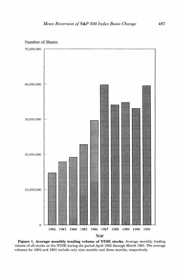
The positive autocorrelation in the fifteen-minute S&P 500 index level changes has dropped over the sample period from 0.507 in the first year, 1983, to only 0.054 in 1990, the last full year. The average monthly trading volume of stocks on the NYSE has also increased dramatically over the same period, as can be seen from Figure 1, suggesting that the rise in stock market trading volume has reduced the effects of infrequent trading on autocorrela- tion in the index.
The S&P 500 futures stay open until 3:15 P.M., fifteen minutes later than the stock market, but prices from both markets are needed to compute the basis.
'About ninety percent of the stocks in the S&P 500 index trade on the NYSE. Stoll and Whaley (1990a, p. 49) report that in 1986 the average time until the first trade of the day for NYSE stocks was 15.46 minutes. S&P 500 stocks tend to be more active than average, however. For the 500 most active stocks on the NYSE, the average time until the first trade was about five minutes.
This effect was first recognized by Fisher (1966). Subsequently, formal nontrading models showing the origins of the positive autocorrelation were developed by Cohen et al. (1978, 19791, Dimson (19791, Lo and MacKinlay (19901, and Stoll and Whaley (1990b1.

The Journal of Finance
Table I
Properties of Observed S&P 500 Basis Changes Estimated first-order autocorrelation ( 6 , ) of observed S&P 500 index changes ( so ) , S&P 500 futures price changes ( f O ) , S&P 500 index basis changes (b" ) , estimated contemporaneous correlation ( f i g ) , and the ratio of the estimated standard deviations ( R O )of observed futures price changes to index level changes computed over 15-, 30-, and 60-minute intervals. Only price changes of the nearby futures contract with more than five days to expiration are used. Overnight price changes and the first price changes each day are excluded. The sample period extends from April 21, 1982 through March 31, 1991.
Period No. of
Begins Ends Observations
15-minute price changes 4/82 3/91 4/82 12/82 1/83 12/83 1/84 12/84 1/85 12/85 1/86 12/86 1/87 12/87 1/88 12/88 1/89 12/89 1/90 12/90 1/91 3/91
30-minute price changes 4/82 3/91 4/82 12/82 1/83 12/83 1/84 12/84 1/85 12/85 1/86 12/86 1/87 12/87 1/88 12/88 1/89 12/89 1/90 12/90 1/91 3/91
60-minute price changes 4/82 3/91 4/82 12/82 1/83 12/83 1/84 12/84 1/85 12/85 1/86 12/86 1/87 12/87 1/88 12/88 1/89 12/89 1/90 12/90 1/91 3/91
51,323 3,913 5,544 5,566 5,673 6,063 5,944 6,059 5,670 5,549 1,342
25,648 1,956 2,772 2,783 2,837 3,031 2,970 3,029 2,827 2,772
671
12,128 889
1,260 1,265 1,325 1,513 1,482 1,513 1,315 1,261
305
Meun Rez?erszon of S&P 500 Index Busis Chu~zge
Number of Shares
50,000,000
Year Figure 1. Average monthly trading volume of NYSE stocks. Average monthly trading
volume of all stocks on the IWSE during the persod April 1982 through March 1991. The average volumes for 1982 and 1991 include only nine months and three months, respectively.
488 The Journal of Finance
Second, and in contrast to the index itself, fifteen-minute price changes in the index futures contract show little autocorrelation. For the overall period, the first-order autocorrelation is not only small, but is slightly negative, -0.029, reflecting almost surely the very narrow bid-ask spread in the S&P 500 futures market. The variance attributable to new information completely swamps the serial covariance attributable to the bid-ask price effect.
Third, the contemporaneous correlation between observed price changes in the index and index futures increases with the length of the trading interval. The contemporaneous correlation for the overall sample period increases from 0.683 to 0.892, for example, as the trading interval increases from fifteen minutes to sixty minutes. The longer the time interval, the less important are the infrequent trading and bid-ask price effects relative to the price change attributable to new information. Increased trading activity in both the stock and futures markets over the years has also increased the contemporaneous correlation between price changes in the two markets. The sixty-minute results show contemporaneous correlation of 0.770 in 1983 and 0.913 in 1990.
Fourth, the ratio of the standard deviations of observed futures price changes to observed index price changes, RO,is greater than one for the overall sample period and for each individual year during the sample period. Observed changes in the futures price are thus, on average, more volatile than changes in the index level.''
Finally, and most important, Table I shows persistent negative first-order autocorrelation in the basis changes of the S&P 500 index. For the fifteen- minute basis changes, the autocorrelation is -0.369 for the entire sample period, and increases from -0.098 in 1982 to -0.424 in 1991 in spite of increased trading volume in both the stock and futures markets. Lengthening the interval, moreover, does not reduce the negative autocorrelation. In fact, the autocorrelation is higher in recent years for the sixty-minute interval than it is for the fifteen-minute interval (e.g., -0.478 versus -0.424 in 1990). Clearly, neither increased trading of index stocks nor lengthening the basis change interval has reduced the mean reversion in the observed basis."
C. Basis Changes Within Transaction Cost Bands
To see whether and to what extent the observed negative autocorrelation in basis changes can be traced to the actions of index arbitragers, we perform two experiments. The first examines basis and mispricing changes after eliminating all pairs of consecutive price changes in which the absolute value
Our standard deviation ratios are higher than those implied by MacKinlay and Ramaswamy (19881, because we use price changes from the last three months of the futures contract life, whereas MacKinlay and Ramaswamy use price changes from all days during the contract life. S&P 500 futures with times to expiration greater than ninety days are thinly traded-in fact, they may not trade for hours or a t all during a trading day. Since intervals with no transaction are recorded as zero price changes, the MacKinlay and Ramaswamy estimate of the variance of futures returns is downward biased as is their estimate of the variance ratio.
11As expected, essentially the same test results are obtained for theoretical mispricing changes during the period June 1988 through March 1991.

489 Mean Reversion of S&P 500 Index Basis Change
of the theoretical mispricing (equation (4)) exceeds one-quarter of one percent of the index level a t the end of the first interval. Mispricings outside these transaction cost bands are taken as potential arbitrage opportunities. Subse- quent price changes are thus more likely to be arbitrage induced than when the mispricings are within the transaction cost bands. Note also that the transaction cost filter we apply is conservative. The transaction costs in- curred in executing profitable index arbitrage are likely to exceed the as- sumed one-quarter of one percent.12 Thus, our experiment is biased toward finding no autocorrelation in the basis changes.
Table I1 contains the test results. The low transaction cost filter does substantially reduce the number of price change observations-the number of fifteen-minute changes, for example, falling from 16,135 to 12,708, and by similar proportions for the thirty- and sixty-minute samples. Surprisingly, however, the autocorrelation of the basis changes drops only slightly from -0.416 in the overall sample to -0.360 after excluding all possible profitable arbitrage opportunities. For the longer price change intervals, the drop in correlation after the filter is applied is even smaller.
D. Value Line Results
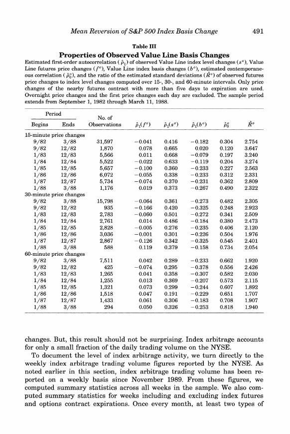
Our second test of the arbitrage explanation of the mean reversion uses data for a different stock index futures contract-one that cannot be arbi- traged against the underlying stock index portfolio. Prior to March 1988, the Value Line futures contract was written on the Value Line Composite Index. Because that index portfolio was geometrically weighted, the possibility of buying or selling a portfolio that behaved like the Value Line index was virtually ruled out.13 Table I11 contains a summary of the empirical proper- ties of the Value Line basis changes during the period when no formal arbitrage was actually being undertaken.
The results for the Value Line basis in Table I11 are remarkably similar to those reported earlier for the S&P 500 basis in Table I. Overall, the futures price changes are mildly negatively autocorrelated, and the stock index level changes are highly positively autocorrelated. Most important, the basis changes show high first-order negative autocorrelation-behavior that can- not be attributed to index arbitrage.
E. Index Arbitrage Trading Volume
Taken together, then, the Value Line and transaction cost band tests imply that formal arbitrage cannot explain the negative autocorrelation in basis
12 Neal (1992) examines actual index arbitrage programs during the first quarter of 1989 and estimates that transaction costs are 0.31 percent (i.e., 0.90 index points divided by 290.50, the average level of the S&P 500 index during his sample period).
I3 Strictly speaking, it is possible to hedge a geometrically weighted portfolio, as shown by Satchel1 and Yoon (1992). For the Value Index, however, that is not practical. Note also that arbitrage is also virtually impossible in the Chicago Board of Trade's Municipal Bond Futures Index contract, where Huggins (1991) reports substantial negative autocorrelation in basis changes.

Table I1
Properties of Observed S&P 500 Basis Changes and Observed Changes in S&P 500 Futures Mispricings
Estimated first-order autocorrelation (6,) of S&P 500 index level changes (so), futures price changes ( f " ) , basis changes ( b O ) ,theoretical futures price changes ( p ) , changes in theoretical futures mispricing (mO),estimated contemporaneous correlation (;:I, and the ratio of the estimated standard deviations ( R O ) of observed futures price changes-index level changes and of futures price changes-theoretical futures price changes computed over 15 , 30-, and 60-minute trading sessions. Only price changes of the nearby futures contract with more than five days to expiration are used. Overnight price changes and the first price changes a t the beginning of each day are excluded. The sample period extends from June 1, 1988 through March 31, 1991. Price changes based on mispricings of greater than I/, percent are eliminated.
Period
No. of
Basis Changes
No. of
Changes in Theoretical Mispricings 2
Begins Ends Observations Observations
15-minute price changes 6/88 3/91 16,135 6/88 12/88 3,574 1/89 12/89 5,670 1/90 12/90 5,549 1/91 3/91 1,342
30-minute price changes 6/88 3/91 8,057 6/88 12/88 1,787 1/89 12/89 2,827 1/90 12/90 2,772 1/91 3/91 671
60-minute price changes 6/88 3/91 3,774 6/88 12/88 893 1/89 12/89 1,315 1/90 12/90 1,261 1/91 3/91 305
Mean Reversion of S&P 500 Index Basis Change 491
Table 111
Properties of Observed Value Line Basis Changes Estimated first-order autocorrelation ( j , ) of obsemed Value Line index level changes ( s o ) ,Value Line futures price changes ( f " ) , Value Line index basis changes ( b o ) ,estimated contemporane- ous correlation ( j,"), and the ratio of the estimated standard deviations ( R o )of obsemed futures price changes to index level changes computed over 15-, 30-, and 60-minute intervals. Only price changes of the nearby futures contract with more than five days to expiration are used. Overnight price changes and the first price changes each day are excluded. The sample period extends from September 1, 1982 through March 11, 1988.
Period No. of
Begins Ends Obsemations
15-minute price changes 9/82 3/88 31,597 9/82 12/82 1,870 1/83 12/83 5,566 1/84 12/84 5,522 1/85 12/85 5,657 1/86 12/86 6,072 1/87 12/87 5,734 1/88 3/88 1,176
30-minute price changes 9/82 3/88 15,798 9/82 12/82 935 1/83 12/83 2,783 1/84 12/84 2,761 1/85 12/85 2,828 1/86 12/86 3,036 1/87 12/87 2,867 1/88 3/88 588
60-minute price changes 9/82 3/88 7,511 9/82 12/82 425 1/83 12/83 1,265 1/84 12/84 1,255 1/85 12/85 1,321 1/86 12/86 1,518 1/87 12/87 1,433 1/88 3/88 294
changes. But, this result should not be surprising. Index arbitrage accounts for only a small fraction of the daily trading volume on the NYSE.
To document the level of index arbitrage activity, we turn directly to the weekly index arbitrage trading volume figures reported by the NYSE. As noted earlier in this section, index arbitrage trading volume has been re- ported on a weekly basis since November 1989. From these figures, we computed summary statistics across all weeks in the sample. We also com- puted summary statistics for weeks including and excluding index futures and options contract expirations. Once every month, a t least two types of

492 The Journal o f Finance
index derivatives expire. Once every quarter, the week also includes the S&P 500 futures contract expiration. Since most index arbitrage activity in the United States is done in conjunction with the S&P 500 futures, we can expect to find particularly high index arbitrage activity in the quarterly expiration cycle.
Table IV shows two important results. First, the amount of index arbitrage activity as a proportion of total program trading varies considerably. Table IV
Table IV
Summary of Weekly NYSE Index Arbitrage, Program Trading, and Total Trading Volume During November 1989 through
March 1991 Summary statistics are computed across all weeks in the sample, all weeks with a nonquarterly expiration day, all weeks with a quarterly expiration day, and all weeks with no expiration day.
Index Average Daily Volume Arbitrage
(in millions) Percentage of All Trading as Percentage All All of All
Summary Index Program All Index Program Program Statistics Arbitrage Trading Trading Arbitrage Trading Trading
All weeks No, of weeks 73 73 Mean 7.2 16.5 Median 6.8 14.7 Minimum 1.1 5.1 Maximum 17.6 39.9 Standard deviation 3.4 7.3
Nonquarterly expiration-day weeks No. of weeks 11 11 Mean 9.0 21.1 Median 8.3 20.2 Minimum 3.0 11.6 Maximum 16.6 31.0 Standard deviation 4.0 6.1
Quarterly expiration-day weeks No. of weeks 6 6 Mean 14.5 34.7 Median 14.4 35.8 Minimum 12.0 25.5 Maximum 17.6 39.9 Standard deviation 2.1 4.8
Weeks not including an expiration day No. of weeks 56 56 Mean 6.0 13.6 Median 6.3 13.7 Minimum 1.1 5.1 Maximum 9.7 20.8 Standard deviation 2.0 3.5
Mean Reversion of ShP 500 Index Basis Change
shows that while index arbitrage accounts for about 43 percent of program trading on average, some weeks it is as low as low as 13.9 percent of all program trading; other weeks it is as much as 64.7 percent. Many studies use program trading volume as a proxy for the amount of index arbitrage. The reported variation implies that this can be a misleading practice. Second, index arbitrage trading volume is a very small percentage of total trading volume on the exchange. Across all weeks in the sample period, index arbitrage accounts for 4.4 percent of total NYSE trading volume. As expected, the index arbitrage activity is higher than average in the expiration weeks-8.6 percent for the "triple-witching days" and 5.3 percent for the "double-witching" days. Since that index arbitrage activity reflects position unwinding, we can reasonably exclude these weeks when assessing the degree of profit-motivated index arbitrage activity. Looking to the last panel of Table IV, we find that index arbitrage accounts for only 3.8 percent of total trading volume. Something other than index arbitrage must be driving the mean reversion in the observed basis levels.
111. Market Microstructure Explanation
What then does cause the mean reversion in the observed stock index futures basis? In this section, we argue that the observed basis change behavior arises because index stocks do not trade continuously. The nature of the mean reversion is complex and depends on a number of factors including the variances of futures price and index level changes, the contemporaneous correlation between futures price changes and changes in the index level, and the frequency of trading of index stocks. For the range of parameters typically associated with intraday stock index-futures price changes, we show that mean reversion not only is expected but also becomes more severe as trading frequency increases (but is not yet continuous).
A. Infrequent Trading and Other Microstructural Considerations
Infrequent trading has two forms. The first occurs when stocks trade every consecutive interval, but not necessarily at the close of each interval. This form of infrequency, often dubbed "nonsynchronous trading," has been stud- ied by Scholes and Williams (1977a, 197713) and Muthuswamy (1990). Infre- quent trading is also said to occur when stocks do not trade every consecutive interval. Fisher (1966), Dimson (1979), Cohen et al. (1978, 1979), Lo and MacKinlay (1990), and Stoll and Whaley (1990b) focus on this "nontrading" and its consequences.
The key to distinguishing nonsynchronous trading from nontrading is the interval over which price changes or returns are computed. When returns are measured on a monthly basis, for example, virtually all NYSE stocks will have traded a t least once, but not all stocks will have transacted exactly a t the close of trading on the last trading day of the month. That is nonsyn- chronous trading. When returns are measured over trading intervals as short
494 The Journal of Finance
as fifteen minutes, however, all NYSE stocks are unlikely to have traded at least once in every consecutive fifteen-minute interval. That is nontrading. As the trading interval shrinks, nonsynchronous trading becomes nontrading.
Before modeling the effects of infrequent trading on observed index level changes, some other microstructure effects that may influence the properties of security returns are also worth noting. Possible contamination in the true price process may arise, for example, from the random bouncing of transac- tion prices between bid and ask levels. Roll (1984) shows that bid-ask price bounce induces negative first-order autocorrelation in observed price changes even though price innovations are serially independent. In the context of this paper, the bid-ask price bounce will show up more strongly in the futures. Because the index level is an average of prices across stocks at a given point in time, the trading by some stocks traded most recently at bid prices is offset by other stocks trading most recently at ask levels.14 The futures contract, on the other hand, is a single security. Negative first-order autocorrelation in observed price changes is likely for extremely short intervals where the price movement attributable to new information may be small relative to the size of the bid-ask spread.
Besides bid-ask bounce, individual security return series may be influenced by the splitting of large buy and sell orders into two or more smaller orders. When split transactions are executed at successively higher (lower) prices, observed price changes may be positively autocorrelated. And, when security returns from different markets are compared, nonuniform delays in recording (and time stamping) transactions may attenuate otherwise perfect cross-correlation. At the portfolio level, delays may also be introduced, because reported stock transaction prices must be further manipulated in computing the S&P 500 index level.15 Finally, another consideration is mechanical failure. In his analysis of apparent delinkage between the S&P 500 futures market and the stock market on October 19, 1987, Kleidon (1992) showed that the computation of the basis was distorted by mechanical failures in the equipment for entering and removing limit orders.
Though a number of microstructure considerations can thus affect the behavior of observed basis price changes, the preponderance of past evidence indicates that intraday security price changes are negatively autocorrelated, while index level changes are positively autocorrelated. This means that the primary microstructure effects are infrequent trading of index stocks and bid-ask bounce for futures. We now try to capture their effects in simple, parsimonious time series models, which help identify the sources of the predictable patterns in observed basis changes.
14 Stoll and Whaley (1990b, pp. 451-452) develop this argument more fully. 15 Delays in computing the S&P 500 index level, once the stock transactions have been entered
on the floor of the NYSE, are minimal. The process by which the index is computed and disseminated is provided in Stoll and Whaley (1990b, p. 445, footnote 6).
495 Mean Reversion of S&P 500 Index Basis Change
B. Dynamics of Observed Index and Futures Price Changes
To model the effects of nonsynchronous trading and nontrading of index portfolio stocks on the observed changes in the index level, we use a modified AR(1) process,
where st is the true index level innovation, st" is the observed index level change, and the parameter 6 measures the degree of trading infrequency.16 The value of $ is assumed to lie between zero and one. As 6 approaches zero, trading becomes perfectly continuous. The observed change in the index level then fully captures the contemporaneous true index innovation s t , which is assumed to be a mean zero, serially uncorrelated shock variable with a homoskedastic variance, aS2.l7 At the other extreme, as $ approaches one, infrequent trading of index stocks becomes increasingly severe. The last trade for a typical stock in the index took place in some previous period. In fact, the structure of equation (5) implies that some stocks may not have traded for many periods, though the likelihood of that event declines geometrically with the order of the lag.
The process governing observed futures price changes is modeled differ- ently. Because the futures contract is a single security, its observed price changes are not smoothed by infrequent trading of the component stocks. Observed futures prices, on the other hand, may appear to bounce as succes- sive transactions are executed at bid and ask price levels. Roll (1984) shows that the bid-ask bounce induces negative serial covariance in the observed price changes series. This bounce can be modeled as an MA(1) process,
f,"= ft + eft-1, (6)
where ft is the true futures price innovation, f," is the observed index level change, and I9 is the bid-ask bounce parameter. The innovation ft is assumed to be a mean zero, serially uncorrelated shock variable with a homoskedastic variance, af2 The bid-ask bounce parameter is negative and has the range -1< I9 < 0. Holding other factors constant, the larger the bid-ask spread, the greater the absolute value of 19.
C. Observed Price Change Variances
The models of the observed index level and the observed futures price changes (equations (5) and (6)) help identify certain characteristics of the variance of observed price changes. The variance of observed changes in the
l6Appendix A contains the derivation of the modified AR(1) process. The qualifier, "modified," is used, because the lagged error term does not have the standard coefficient of one. The modified process is computationally equivalent, of course, to a standard AR(1).
l7 The zero mean assumption is made for algebraic convenience only. None of the subsequent results rely on this assumption.
The Journal of Finance
stock index level, for example, is
(See Appendix B.) Note that the variance of the observed index level changes, as!, is always less than the variance of the true index level innovations, as2, as long as the infrequency parameter is within its defined range (i.e., 0 < (b < 1). Observed stock prices, being last reported transaction prices, often trail actual market movements and therefore smooth the movements of the ob- served index level. This smoothing of index level changes reduces observed volatility relative to true volatility. To illustrate the relative size of the variance of observed index level changes, consider the autocorrelation esti- mate of 0.128 reported for the fifteen-minute interval in Table I. Using this value to approximate (b, the variance of' observed index level changes under- states the true value by nearly 23 percent.
Thc variance of the observed changes in the futures price is
Since the variance of the observed futures price changes, a;, is the sum of two components-the variance of true price changes and the variance of the price movements from bid to ask levels-the variance of the observed futures price changes index is greater than the variance of the true futures price changes as long as the bid-ask spread in the futures market is econoinically significant (i.e., 0 < 0). The larger is the bid-ask spread, the greater is a:. The estimated first-order autocorrelation of futures price changes reported earlier in Table I, however, shows that the effect of the bid-ask spread is trivial. The autocorrelation using fifteen-minute price changes (where the bid-ask price effect should be greatest) is -0.029 over the entire sample period. In other words, the variance of observed futures price changes is only about 0.08 percent larger than the true variance.''
Taken together, relations equations (7) and (8) imply that the ratio of the variance of observed futures price changes to variance of observed index level
changes, (RO)' = is greater than one where the variances of the innova- a*!'
tions of the futuresoand the index are, in fact, equal (i.e., af2 = as2).
PROPOSITION1: If the bid-ask spread in the futures m.arket is economically significant (0 < O), i f the stocks within the index portfolio trade infrequently (4 > O), and if the innovations of the futures and the index have the same variance (a; = a:), the variance ratio of observed futures price changes to observed index level changes is greater than one.
l8The first-order autocorrelation of the observed futures price changes is 0/(1 + 0'). Equating this expression to -0.029 and solving, we find that 0 is -0.02902 and hence (1 + 0 is 1.0008.

Mean Reversion of S&P 500 Index Basis Change
Proof of Proposition 1: Since 4 > 0, the variance ratio is
Q.E.D.
In other words, microstructure effects alone can cause the variance ratio of observed futures price changes to observed index level changes to exceed one.
The evidence reported in Table I is consistent with Proposition 1.All of the reported standard deviation (variance) ratios of the observed price changes, R O ,exceed one, independent of the interval length and sample period. Since the autocorrelation of the futures price changes is near zero as noted above, the standard deviation ratio results imply that the infrequent trading of stocks within the index portfolio is a more serious concern than the bid-ask price effect in the futures.
D. Dynamics of Observed Basis Changes
We turn now to the primary concern of this study-the autocorrelation of changes in the observed basis, bp = f e - sp. In particular, we show that our simple microstructure models (equations (5) and (6)) can explain not only the mean reversion in the observed basis but also the increase in mean reversion that has been experienced in recent years.
The first-order autocorrelation coefficient of bp is defined below:
PROPOSITION autocorrelation of observed basis changes in 2: The first-order terms of the true underlying parameters is
Proof of Proposition 2: See Appendix B.
If the bid-ask spread in the futures market is economically insignificant (6 = 0) and if the stocks within the index portfolio trade continuously (4 = 0), the numerator in equation (9) and hence the first-order autocorrelation of observed basis changes are zero. First-order autocorrelation vanishes only where the microstructure effects of bid-ask spreads and infrequent trading are absent.
498 The Journal of Finance
Equation (9) shows that the first-order autocorrelation of observed basis changes is a function of the five parameters 4 , 8, of, as, and of,. For greater insight into the meaning of Proposition 2, we recast equation (9) in terms of the contemporaneous correlation instead of contemporaneous covariance and then reduce the parameter space. Substituting the correlation expression, ats = Pfsfffas, we get
Next, we simplify. To begin, we assume that the variance of true futures price innovations equals the variance of true index innovations (i.e., af2 and that the futures price innovations and true index level innovations are perfectly positively correlated (i.e., pfs = + 1). Indeed, if the riskless rate of interest and the dividends on the stock index portfolio are certain, the absence of costless arbitrage opportunities in the marketplace will ensure that these conditions hold. Also, given the absence of meaningful autocorrela- tion in the observed futures price changes, we assume 8 = 0.
PROPOSITIOX3: If the bid-ask spread in the futures market is economically insignificant (8 = 01, if the stocks within the index portfolio trade infrequently ( 4 > O), and i f the innovations of the futures and the index have the same variance (of2 = .us2)and are perfectly positively correlated ( pfs = + l), the first-order autocorrelation of observed basis changes is
Proof of Proposition 3: See Appendix B.
Proposition 3 implies that the first-order autocorrelation in observed basis changes is always negative over the admissible range of values for the infrequency parameter (i.e., 0 < 4 < 1). Where 4 = 0 and hence is outside the admissible range, the variance of the basis changes is zero,lg so the autocorrelation changes are undefined. Proposition 3 also implies that as 4 becomes small the autocorrelation in basis changes becomes more negative. Apparently, infrequent trading has relatively less effect on the serial covari- ance of observed basis changes than it does on the variance. In sum, under plausible assumptions about the true, but unobservable, stock index futures basis (i.e., uf = as and pfs = + I), spurious mean reversion in the basis is the
To see this, set 0 = 4 = 0, pp = + 1,and rrf = nS in the denominator of equation (11).
0:) =
499 Mean Reversion of S&P 500 Index Basis Change
rule rather than the exception. Moreover, the mean reversion becomes greater as the frequency of stock market trading increases!
Now, we relax the certainty assumptions regarding the interest rate and the dividends of the index portfolio. If the interest rate or the dividends are uncertain, the standard deviation of the futures price innovations will exceed the standard deviation of the index innovations (i.e., af> a,) and the contem- poraneous correlation between the innovations of the futures and the index will be less than one (i.e., pfs < I)." To provide greater generality in our results, therefore, we write equation (10) as follows:
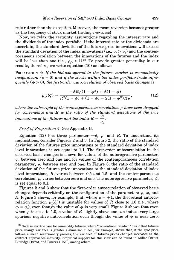
PROPOSITION4: If the bid-ask spread in the futures market is economically insignificant (%= 0) and if the stocks within the index portfolio trade infre- quently ( 4 > O), the first-order autocorrelation of observed basis changes is
where the subscripts of the contemporaneous correlation p have been dropped for convenience and R is the ratio of the standard deviations of the true
innovations of the futures and the index R = -.uf as
Proof of Proposition 4: See Appendix B.
Equation (12) has three parameters-8, p , and R . To understand its implications, consider Figures 2 and 3. In Figure 2, the ratio of the standard deviation of the futures price innovations to the standard deviation of index level innovations is set equal to 1.1.The first-order autocorrelation in the observed basis changes is shown for values of the autoregressive parameter, #, between zero and one and for values of the contemporaneous correlation parameter, p, between zero and one. In Figure 3, the ratio of the standard deviation of the futures price innovations to the standard deviation of index level innovations, R , varies between 0.5 and 1.5, and the contemporaneous correlation, p, varies between zero and one. The autoregressive parameter, 4, is set equal to 0.1.
Figures 2 and 3 show that the first-order autocorrelation of observed basis changes depends critically on the configuration of the parameters p, +, and R. Figure 3 shows, for example, that, where p = +1, the theoretical autocor- relation function p,(bp) is unstable for values of R close to 1.0 (i.e., where crf = a,), even though the value of # is very small. Figure 2 shows that even when p is close to 1.0, a value of R slightly above one can induce very large spurious negative autocorrelation even though the value of + is near zero.
20 Such is also the case for commodity futures, where "conventional wisdom" has it that futures price change variance is greater. Samuelson (19761, for example, shows that, if the spot price follows a mean reversionary process, the variance of futures prices changes increases as the contract approaches maturity. Empirical support for this view can be found in Miller (19791, Rutledge (19761, and Powers (19701, among others.

500 The Journal of Finance
Figure 2. First-order autocorrelation as a function of the infrequent trading and contemporaneous correlation. First-order autocorrelation of observed basis changes, p,(bp), as a function of the infrequent trading parameter, 4, and the contemporaneous correlation between innovations to the stock index level and the futures price innovation, p. The ratio of the standard deviation of the futures price innovation to the standard deviation of the index level innovation, R, equals 1.1.The values of p and 4 range between 0 and 1.
Figures 2 and 3 also show that our modeled microstructure effects can even produce positive autocorrelation in the observed basis changes, though only in the parameter regions where the contemporaneous correlation between the index and the futures, p, is low and/or where the ratio of the standard deviations, R , is less than one. For the S&P 500 futures basis, neither of these conditions is realistic.
An important implication of Figures 2 and 3 is that strong negative first-order autocorrelation in observed basis changes may be observed even when stocks i n the index portfolio trade nearly continuously (i.e., 4 = 0, but 4 + 0). When positive contemporaneous correlation p is coupled with values of the standard deviation ratio R in excess of one, strong negative first-order autocorrelation arises. Because infrequent trading of the stocks in the index
501 Mean Reversion of S&P 500 Index Basis Change
1 0.4 Figure 3. First-order autocorrelation as a function of contemporaneous correlation
and the ratio of standard deviations. First-order autocorrelation of observed basis changes, pl(by), as a function of the contemporaneous correlation between the innovations to the stock index level and the futures price, p, and the ratio of the standard deviation of the futures price innovation to the standard deviation of the index level innovation, R. The infrequent trading parameter, 4, equals 0.1. The value of p ranges between 0 and 1, and the value of R ranges between 0.5 and 1.5.
portfolio is well documented (i.e., 0 << 4 < I), negative and significant values of first-order autocorrelation in the observed basis changes p,(bP) are to be expected. The predicted mean reversion is merely a statistical artifact, how- ever, and has nothing to do with the actions of index arbitragers.
E. Observed Autocorrelation in Terms of Observed Parameters
Propositions 2 and 4 express the first-order autocorrelation of observed basis changes in terms of the true (unobserved) parameters af, a,, and pf,. While theory guides us as to plausible values for the contemporaneous correlation, p , and for the ratio of the standard deviations, R , expressing the
502 The Journal of Finance
functional forms of the propositions in terms of the directly observable parameters, a , ~ , and pfoso, is also useful.
The analogue to Proposition 2 in terms of the observable parameters is:
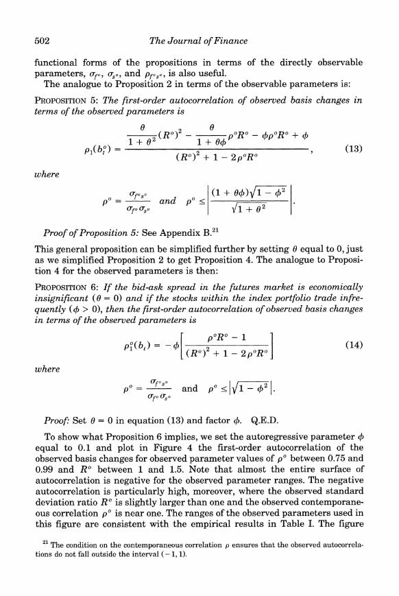
PROPOSITION5: The first-order autocorrelation of observed basis changes i n terms of the observed parameters is
where
= -f f f o s o and pO_< ff-0 f f s o
Proof of Proposition 5: See Appendix B."
This general proposition can be simplified further by setting 0 equal to 0, just as we simplified Proposition 2 to get Proposition 4. The analogue to Proposi- tion 4 for the observed parameters is then:
PROPOSITION6: I f the bid-ask spread in the futures market is economically insignificant (0 = 0) and if the stocks within the index portfolio trade infre- quently ( 4 > 01, then the first-order autocorrelation of observed basis changes in terms of the observed parameters is
where
fffosoPo = - and pOs l \ l m 1ff,,
Proofi Set 8 = 0 in equation (13) and factor 4. Q.E.D.
To show what Proposition 6 implies, we set the autoregressive parameter 4 equal to 0.1 and plot in Figure 4 the first-order autocorrelation of the observed basis changes for observed parameter values of pObetween 0.75 and 0.99 and RO between 1 and 1.5. Note that almost the entire surface of autocorrelation is negative for the observed parameter ranges. The negative autocorrelation is particularly high, moreover, where the observed standard deviation ratio RO is slightly larger than one and the observed contemporane- ous correlation pO is near one. The ranges of the observed parameters used in this figure are consistent with the empirical results in Table I. The figure
21 The condition on the contemporaneous correlation p ensures that the observed autocorrela- tions do not fall outside the interval ( - 1,l).
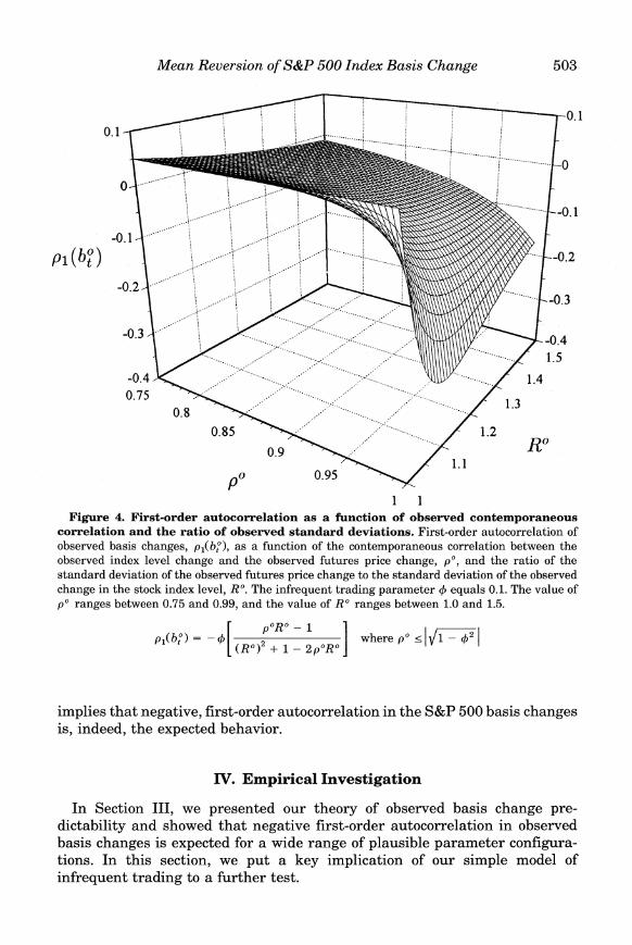
503 Mean Reversion of S&P 500 Index Basis Change
1 1 Figure 4. First-order autocorrelation as a function of observed contemporaneous
correlation and the ratio of observed standard deviations. First-order autocorrelation of observed basis changes, p,(be), as a function of the contemporaneous correlation between the observed index level change and the observed futures price change, p o , and the ratio of the standard deviation of the observed futures price change to the standard deviation of the observed change in the stock index level, Ro.The infrequent trading parameter 4 equals 0.1. The value of pO ranges between 0.75 and 0.99, and the value of Ro ranges between 1.0 and 1.5.
implies that negative, first-order autocorrelation in the S&P 500 basis changes is, indeed, the expected behavior.
IV. Empirical Investigation
In Section 111, we presented our theory of observed basis change pre- dictability and showed that negative first-order autocorrelation in observed basis changes is expected for a wide range of plausible parameter configura- tions. In this section, we put a key implication of our simple model of infrequent trading to a further test.
504 The Journal of Finance
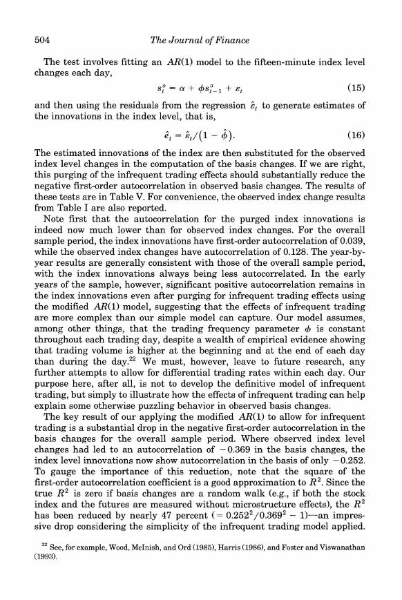
The test involves fitting an AR(1) model to the fifteen-minute index level changes each day,
s,O = a + + st (15)
and then using the residuals from the regression i., to generate estimates of the innovations in the index level, that is,
The estimated innovations of the index are then substituted for the observed index level changes in the computation of the basis changes. If we are right, this purging of the infrequent trading effects should substantially reduce the negative first-order autocorrelation in observed basis changes. The results of these tests are in Table V. For convenience, the observed index change results from Table I are also reported.
Note first that the autocorrelation for the purged index innovations is indeed now much lower than for observed index changes. For the overall sample period, the index innovations have first-order autocorrelation of 0.039, while the observed index changes have autocorrelation of 0.128. The year-by- year results are generally consistent with those of the overall sample period, with the index innovations always being less autocorrelated. In the early years of the sample, however, significant positive autocorrelation remains in the index innovations even after purging for infrequent trading effects using the modified AR(1) model, suggesting that the effects of infrequent trading are more complex than our simple model can capture. Our model assumes, among other things, that the trading frequency parameter $ is constant throughout each trading day, despite a wealth of empirical evidence showing that trading volume is higher at the beginning and at the end of each day than during the day." We must, however, leave to future research, any further attempts to allow for differential trading rates within each day. Our purpose here, after all, is not to develop the definitive model of infrequent trading, but simply to illustrate how the effects of infrequent trading can help explain some otherwise puzzling behavior in observed basis changes.
The key result of our applying the modified AR(1) to allow for infrequent trading is a substantial drop in the negative first-order autocorrelation in the basis changes for the overall sample period. Where observed index level changes had led to an autocorrelation of -0.369 in the basis changes, the index level innovations now show autocorrelation in the basis of only -0.252. To gauge the importance of this reduction, note that the square of the first-order autocorrelation coefficient is a good approximation to R2. Since the true R2 is zero if basis changes are a random walk (e.g., if both the stock index and the futures are measured without microstructure effects), the R2 has been reduced by nearly 47 percent (= 0.2522/0.3692 - 1)-an impres-sive drop considering the simplicity of the infrequent trading model applied.
22 See, for example, Wood, McInish, and Ord (19851, Harris (19861, and Foster and Viswanathan (19931.
--
---
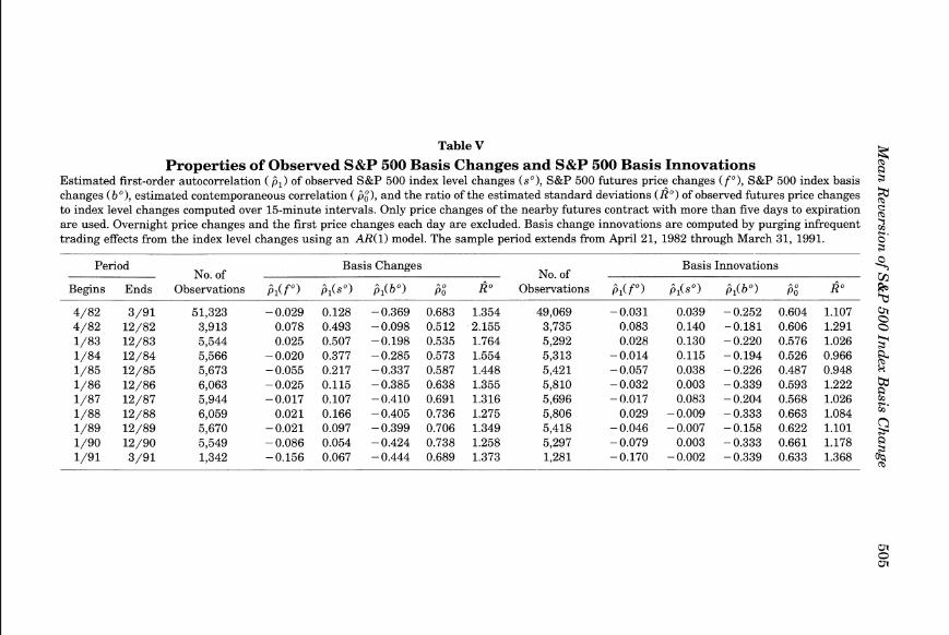
TableV %Properties of Observed S&P 500 Basis Changes and S&P 500 Basis Innovations i2
Estimated first-order autocorrelation ( f i , ) of observed S&P 500 index level changes ( s o ) ,S&P 500 futures price changes ( f o ) ,S&P 500 index basis 3
changes (b" ) ,estimated contemporaneous correlation ( fi:), and the ratio of the estimated standard deviations ( R o )of observed futures price changes $ to index level changes computed over 15-minute intervals. Only price changes of the nearby futures contract with more than five days to expiration are used. Overnight price changes and the first price changes each day are excluded. Basis change innovations are computed by purging infrequent 2 trading effects from the index level changes using an AR(1) model. The sample period extends from April 21, 1982 through March 31, 1991. F'
3
Period No. of
Basis Changes No. of
Basis Innovations Qm
Begins Ends Observations j,( f " ) fil(sO) fil(bo) j," R" Observations jl( fo) j l ( so ) j l (bo) j: R . @
4/82 3/91 51,323 0 . 0 2 9 0.128 -0.369 0.683 1.354 49,069 0 . 0 3 1 0.039 0 . 2 5 2 0.604 1.107 "n3
4/82 12/82 3,913 0.078 0.493 -0.098 0.512 2.155 3,735 0.083 0.140 -0.181 0.606 1.291 0
1/83 12/83 5,544 0.025 0.507 -0.198 0.535 1.764 5,292 0.028 0.130 -0.220 0.576 1.026 3 1/84 12/84 5,566 0 . 0 2 0 0.377 -0.285 0.573 1.554 5,313 0 . 0 1 4 0.115 0 . 1 9 4 0.526 0.966 1/85 12/85 5,673 -0.055 0.217 0 . 3 3 7 0.587 1.448 5,421 0 . 0 5 7 0.038 0 . 2 2 6 0.487 0.948 1/86 12/86 6,063 -0.025 0.115 -0.385 0.638 1.355 5,810 -0.032 0.003 -0.339 0.593 1.222 $ 1/87 12/87 5,944 0 . 0 1 7 0.107 0 . 4 1 0 0.691 1.316 5,696 0 . 0 1 7 0.083 0 . 2 0 4 0.568 1.026 g. 1/88 12/88 6,059 0.021 0.166 0 . 4 0 5 0.736 1.275 5,806 0.029 -0.009 -0.333 0.663 1.084 " 1/89 12/89 5,670 0 . 0 2 1 0.097 -0.399 0.706 1.349 5,418 -0.046 0 . 0 0 7 -0.158 0.622 1.101 9 1/90 12/90 5,549 -0.086 0.054 0 . 4 2 4 0.738 1.258 5,297 0 . 0 7 9 0.003 0 . 3 3 3 0.661 1.178 Q
1/91 3/91 1,342 -0.156 0.067 -0.444 0.689 1.373 1,281 -0.170 -0.002 -0.339 0.633 1.368 5
506 The Journal of Finance
The year-by-year results also show reductions in the level of autocorrelation, except for 1982 and 1983, when, as noted earlier, the modified AR(1) model performed less well.
The ratio of the standard deviation of futures price changes to index level changes is also reduced. Where the ratio of observed futures price change standard deviation to index level change standard deviation had been 1.354, the index level innovations now yield a ratio of only 1.107. The high ratio in the raw series had reflected the smoothing of the observed index level series by the infrequent trading of stocks within the index portfolio. When the modified AR(1) model is used to back out the estimated index innovations, the innovations have more volatility than the observed index changes, and the ratio of futures to index standard deviations is reduced.
In summary, even a simple model of infrequent trading such as the modified AR(1) model can control, to a considerable degree, the effects of infrequent trading of the stocks within the index portfolio. With this control in place, the negative first-order autocorrelation in basis changes is notice- ably reduced.
V. Summary and Conclusions
The conventional wisdom is that the mean reversion in the observed stock index basis, documented in many studies, traces to index arbitrage. This study shows, however, that index arbitrage is not the only explanation. We show, in fact, that under reasonable assumptions about infrequent trading of index portfolio stocks, strong negative first-order autocorrelation could be expected even if no formal arbitrage ever occurred. After all, there are people who can trade in both markets, and they can be expected to shift their trading as circumstances warrant.
But, if the predictability of basis changes is mainly a statistical illusion, as we have argued, why do we see so much index arbitrage on the NYSE? (See, for example, Sofianos (1990) and Neal (1992).) The answer, we have shown, is that we don't really see all that much of it. Formal index arbitrage during our sample period accounts for only about four percent of NYSE volume. And such formal arbitrage as we do see appears to serve mainly to counteract the additional drag in index adjustment induced by the very special set of rules that the NYSE imposes to create the impression of continuity in the path of prices. In a pure dealer market such as the spot market in Treasury bonds, no actual arbitrage transactions are needed to keep the spot and futures prices in line. The dealers, upon observing a jump in futures price, would simply mark their own stale quotes up or down to match. An exploitable gap does not emerge, because, effectively, the spot dealers "price off the futures" and hence eliminate any profit opportunity directly.
On the NYSE, by contrast, the specialists normally move their quotes only in response to actual transactions. They are enjoined by the terms of their franchise, moreover, to keep successive prices within one-eighth of the previ-

507 Mean Reversion of S&P 500 Index Basis Change
ous price to the maximum extent feasible. And they do succeed in doing so more than 95 percent of the time even though they may have to face large changes in their own inventories as they walk prices up or down an eighth at a time. The speed of adjustment of prices is slowed also by limit orders of other investors resting in the specialist's book. These orders cannot be made contingent on a jump in the futures price but must specifically be lifted and reset, a process that cannot always be implemented quickly, particularly when trading gets hectic. These institutionally induced lags in the adjust- ment of stock prices to jumps in the futures prices create a gap that fast moving arbitragers can exploit at the expense of the NYSE's specialists and limit-order customers.23
Although these stock market/futures market interactions have been the main focus of this article, essentially the same ingredients can be found in other market settings. The back months of most futures contracts, for exam- ple, are far less liquid than the front months. We suspect, therefore, that changes in calendar spreads (and undoubtedly also in intercommodity spreads) will exhibit the same negative autocorrelation we have documented for basis changes in the S&P500 index.
More generally, our analysis suggests similar elements are likely to creep in whenever the price-change or return series of two securities or portfolios of securities are differenced. Differencing neutralizes the common market fac- tors and highlights the differences in the microstructure of the markets in which they trade. And, as we have seen, even seemingly small differences in trading frequency or other microstructure parameters can seriously distort the statistical characteristics of the differenced series, particularly when returns are measured over very short intervals. This news will hardly be comforting to users of the increasingly available intraday price series. But at least they've been warned.
Appendix A
Derivation of Modified Autoregressive Process for Observed Index Level Changes
This appendix presents the derivation of the modified first-order autore- gressive process that describes observed level changes, that is,
23 Some dealer markets like NASDAQ in the United States or ARIEL in London require dealers to guarantee a minimum size (not always trivially small) a t their posted quotes. Similar guarantees apply in other automatic execution systems like RAES (of the CBOE). To that extent, the dealers or the system face a stale-quote, pick-off problem similar to that a t the NYSE. The much discussed, heavy use of index arbitrage in Japan is of quite a different kind. It appears to be less a matter of arbitraging prices between the spot and futures markets than of arbitraging between the retail stock commissions and the much lower commissions on futures. See Miller (1992).
508 The Journal of Finance
where s, is the true index level change, sy is the observed index level change, and 4 is the trading infrequency parameter (i.e., the higher is 4 , the lower is the frequency with which the stocks in the index trade).
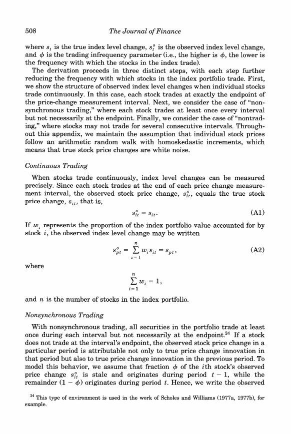
The derivation proceeds in three distinct steps, with each step further reducing the frequency with which stocks in the index portfolio trade. First, we show the structure of observed index level changes when individual stocks trade continuously. In this case, each stock trades at exactly the endpoint of the price-change measurement interval. Next, we consider the case of "non- synchronous trading," where each stock trades at least once every interval but not necessarily at the endpoint. Finally, we consider the case of "nontrad- ing," where stocks may not trade for several consecutive intervals. Through- out this appendix, we maintain the assumption that individual stock prices follow an arithmetic random walk with homoskedastic increments, which means that true stock price changes are white noise.
Continuous Trading
When stocks trade continuously, index level changes can be measured precisely. Since each stock trades a t the end of each price change measure- ment interval, the observed stock price change, s;, equals the true stock price change, sit , that is,
If wirepresents the proportion of the index portfolio value accounted for by stock i , the observed index level change may be written
where
and n is the number of stocks in the index portfolio.
Nonsynchronous Trading
With nonsynchronous trading, all securities in the portfolio trade at least once during each interval but not necessarily at the endpoint.'* If a stock does not trade at the interval's endpoint, the observed stock price change in a particular period is attributable not only to true price change innovation in that period but also to true price change innovation in the previous period. To model this behavior, we assume that. fraction 4 of the ith stock's observed price change si", is stale and originates during period t - 1, while the remainder (1 - 4) originates during period t. Hence, we write the observed
24 This type of environment is used in the work of Scholes and Williams (1977a, 1977131, for example.

509 Mean Reversion of S&P 500 Index Basis Change
stock price change as
If 4 = 0, trading is continuous. The observed price change fully captures the contemporaneous true price change as we saw in equation (A2). At the other extreme, if 4 = 1the last stock trade took place at the endpoint of interval t - 1and all of the observed price change occurs with one lag.25
With each stock's observed price change dynamics described by equation (A3), the observed index level change dynamics can be obtained by applying the index portfolio weights and summing across stocks. Under nonsyn-chronous trading, the observed index level changes may be written
Equation (A4) implies that observed index level changes follow a modified MA(1) process. The term "modified," is used because the lagged index innova- tion has a nonstandard coefficient of 4.
Nontrading
Under nontrading, stocks may not trade for several consecutive intervals. If all stocks traded a t least once every q intervals, the nonsynchronous trading analysis above could be reworked to show that observed index level changes would follow an MA(q) process." Unfortunately, this means that the ob- served index level change process depends on q different parameters, making it unwieldy. A simpler, alternative approach is to adopt a framework similar to equation (A4) above. As in equation (A4), the observed index level change depends on the contemporaneous change in the true index level weighted by 1- 4. In place of having the remaining weight on the lag be one true index level of change, however, we split the weight across an infinite number of lagged true index level changes, with the property that the weights decline geometrically with the order of the lag.27 More specifically, we write the
25 For greater generality, 4 can be made security specific. See, for example, Cohen et al. (1978, 1979) and Dimson (1979).
26 See, for example, Muthuswamy (1990). 27 Lo and MacKinlay (19901, for example, use this approach. The value (1 - 4) can be
interpreted as the probability of a trade taking place in a given interval.

510 The Journal of Finance
observed index level change process as
where the weights attached to the lag true index level changes sum to +. The benefit of invoking this assumption is that the term in squared brackets is simply 4s;. ,-,, which means that the observed portfolio price change process may be written parsimoniously as
Equation (A6) shows that observed index level changes follow a modified AR(1) process. Here the term, "modified," is used because the contemporane- ous innovation term has the coefficient (1 - 4) rather than one.
Appendix B
Proofs of Selected Propositions
Proof of Equation (7):
Q.E.D.
Proof of Proposition 2: First, consider the denominator term,
Var( b;) = Var( f," - s:)
= [a; [a,:+ - 2ups0.
We already have expressions u; and a,? in terms of the variances on the innovations (see equations (7) and (8)). To do the same for the covariance
Mean Reversion of S&P 500 Index Basis Change
term,
ap,, = E ( f,Osp)
= E [ (ft + O f t - , ) ( l - 4 ) ( l- 4 L ) - ' S t ]
= ~ [ ( f ,+ 8 f t - , ) ( l - 4 ) ( s t + +st- , + 42st-2 + ...)I = ( 1 - 4 ) E [ f t s t+ 84ft- ,s t- ,]
= ( 1 - 4 x 1 + 0 4 ) a f s .
Now, consider the numerator term for the lag one autocorrelation coefficient,
Cov(b:, bp-,) = E [ ( f t o- ~ f ) ( f , O - ~- S ~ O - ~ ) ] . Using the lag operator L where ~~x~ = the expression becomes x ~ - ~ ,
Assembling all the component terms and simplifying,
Q.E.D.
Proof of Proposition 3: Setting 8 = 0 and af = a,, equation (10)becomes

512 The Journal of Finance
Multiplying throughout by (1 + +)/as2,
Setting pfs = + 1,
Q.E.D.
Proof of Proposition 4: Setting 8 = 0, equation (10)becomes
Multiplying throughout by (1 + +)/as2and substituting R = -,af as
Q.E.D.
Proof of Proposition 5: Substituting expressions, as2=
a; U f O s O---I + R2, and afs = into equation (9), it follows that (1- +) i i + 0 4 )
Q.E.D.
REFERENCES
Cohen, Kalman J., Steven F. Maier, Robert A. Schwartz, and David K. Whitcomb, 1978, The returns generation process, returns variance, and the effect of thinness in securities mar- kets, Journal ofFinance 33, 149-167.
, 1979, On the existence of serial correlation in an efficient securities market, TIMS Studies in the Management Sciences 11,151-168.
Dimson, Elroy, 1979, Risk measurement when shares are subject to infrequent trading, Journal of Financial Economics 7, 197-226.
Fisher, Lawrence, 1966, Some new stock market indexes, Journal of Business 39, 191-225. Foster, F. Douglas, and S. Viswanathan, 1993, Variations in trading volume, return volatility,
and trading costs: Evidence on recent price formation models, Journal of Finance 48, 187-211.
Mean Reversion of S&P 500 Index Basis Change 5 13
Harris, Lawrence, 1986, A transaction data study of weekly and intradaily patterns in stock returns, Journal of Financial Economics 16, 99-117.
, 1989, The October 1987 S&P 500 stock-futures basis, Journal of Finance 44, 77-99. Huggins, Doug, 1991, An examination of mean reversion in the municipal bond index futures
basis, curriculum paper, Graduate School of Business, University of Chicago. Kleidon, Allan W., 1992, Arbitrage, nontrading and stale prices: October 1987, Journal of
Business 65, 483-507. , and Robert E. Whaley, 1992, One market? Stocks, futures and options during October
1987, Jourizal of Finance 47, 851-877. Lim, Kian-Guan, 1990, Arbitrage and price behavior of Nikkei stock index futures, ~'ournal of
Futures Markets 12, 151-161. Lo, Andrew, and A. Craig MacKinlay, 1990, An econometric analysis of infrequent trading,
Journal of Econometrics 45, 181-211. MacKinlay, A. Craig, and Krishna Ramaswamy, 1988, Index futures arbitrage and the behavior
of stock index futures prices, Reuiew of Financial Studies 1, 137-158. Miller, Katherine Dusak, 1979, The relation between volatility and maturity in futures contracts,
in R. M. Leuthold, ed.: Commodity Markets and Futures Prices (Chicago Mercantile Ex- change, Chicago).
Miller, Merton H., 1989, Equilibrium relations between cash markets and futures markets, Manuscript, Graduate School of Business, University of Chicago.
, 1992, The economics and politics of index arbitrage in the U.S. and Japan, Manuscript, Graduate School of Business, University of Chicago.
Muthuswamy, Jayaram, 1990, Nonsynchronous trading and the index actocorrelation problem, Ph.D. Dissertation, Graduate School of Business, University of Chicago.
Neal, Robert, 1992, Direct tests of index arbitrage models, Working paper, Department of Finance, University of Washington.
Powers, Mark, 1970, Does futures trading reduce price fluctuations in the cash markets?, American Economic Reuiew 60, 460-464.
Roll, Richard, 1984, A simple implicit measure of the effective bid-ask spread, Journal of Finance 39, 1127-1139.
Rutledge, David J. S., 1976, A note on the variability of futures prices, Review of Economics and Statistics 58, 118-120.
Samuelson, Paul, 1976, Is the real-world a tale told by the idiot of chance?, Reuiew of Economics and Statistics 58, 120-123.
Satchell, Stephen E., and Youngjun Yoon, 1992, Can we hedge the FT30 index?, Manuscript, Trinity College and Queens' College, Universiiy of Cambridge.
Scholes, Myron, and Joseph Williams, i977a, Estimating betas from nonsynchronous data, Journal of Financial Economics 5, 309-327.
, 1977b, Estimating betas from daily data, Working paper, Graduate School of Business, University of Chicago.
Sofianos, George, 1990, Index arbitrage profitability, Working paper 90-04, New York Stock Exchange.
Stoll, Hans R., and Robert E. Whaley, 199Oa, Stock market structure and volatility, Review of Financial Studies 3, 37-71.
, 1990b, The dynamics of stock index and stock index futures returns, Journal of Financial and Quantitative Analysis 25, 441-468.
Wood, Robert A,, Thomas H. McInish, and J . Keith Ord, 1985, An investigation of transaction data for NYSE stocks, Journal of Finance 40, 723-741.
Yadav, Pradeep K., and Peter F. Pope, 1990, Stock index futures arbitrage: International evidence, Journal of Futures Markets 10, 573-603.
You have printed the following article:
Mean Reversion of Standard & Poor's 500 Index Basis Changes: Arbitrage-Induced orStatistical Illusion?Merton H. Miller; Jayaram Muthuswamy; Robert E. WhaleyThe Journal of Finance, Vol. 49, No. 2. (Jun., 1994), pp. 479-513.Stable URL:
http://links.jstor.org/sici?sici=0022-1082%28199406%2949%3A2%3C479%3AMROS%26P%3E2.0.CO%3B2-R
This article references the following linked citations. If you are trying to access articles from anoff-campus location, you may be required to first logon via your library web site to access JSTOR. Pleasevisit your library's website or contact a librarian to learn about options for remote access to JSTOR.
[Footnotes]
1 The October 1987 S&P 500 Stock-Futures BasisLawrence HarrisThe Journal of Finance, Vol. 44, No. 1. (Mar., 1989), pp. 77-99.Stable URL:
http://links.jstor.org/sici?sici=0022-1082%28198903%2944%3A1%3C77%3ATO1S5S%3E2.0.CO%3B2-4
5 Arbitrage, Nontrading, and Stale Prices: October 1987Allan W. KleidonThe Journal of Business, Vol. 65, No. 4. (Oct., 1992), pp. 483-507.Stable URL:
http://links.jstor.org/sici?sici=0021-9398%28199210%2965%3A4%3C483%3AANASPO%3E2.0.CO%3B2-V
6 The Dynamics of Stock Index and Stock Index Futures ReturnsHans R. Stoll; Robert E. WhaleyThe Journal of Financial and Quantitative Analysis, Vol. 25, No. 4. (Dec., 1990), pp. 441-468.Stable URL:
http://links.jstor.org/sici?sici=0022-1090%28199012%2925%3A4%3C441%3ATDOSIA%3E2.0.CO%3B2-O
http://www.jstor.org
LINKED CITATIONS- Page 1 of 6 -
NOTE: The reference numbering from the original has been maintained in this citation list.
8 Stock Market Structure and VolatilityHans R. Stoll; Robert E. WhaleyThe Review of Financial Studies, Vol. 3, No. 1, National Bureau of Economic Research Conference:Stock Market Volatility and the Crash, Dorado Beach, March 16-18, 1989. (1990), pp. 37-71.Stable URL:
http://links.jstor.org/sici?sici=0893-9454%281990%293%3A1%3C37%3ASMSAV%3E2.0.CO%3B2-0
9 Some New Stock-Market IndexesLawrence FisherThe Journal of Business, Vol. 39, No. 1, Part 2: Supplement on Security Prices. (Jan., 1966), pp.191-225.Stable URL:
http://links.jstor.org/sici?sici=0021-9398%28196601%2939%3A1%3C191%3ASNSI%3E2.0.CO%3B2-A
9 The Returns Generation Process, Returns Variance, and the Effect of Thinness in SecuritiesMarketsKalman J. Cohen; Steven F. Maier; Robert A. Schwartz; David K. WhitcombThe Journal of Finance, Vol. 33, No. 1. (Mar., 1978), pp. 149-167.Stable URL:
http://links.jstor.org/sici?sici=0022-1082%28197803%2933%3A1%3C149%3ATRGPRV%3E2.0.CO%3B2-C
9 The Dynamics of Stock Index and Stock Index Futures ReturnsHans R. Stoll; Robert E. WhaleyThe Journal of Financial and Quantitative Analysis, Vol. 25, No. 4. (Dec., 1990), pp. 441-468.Stable URL:
http://links.jstor.org/sici?sici=0022-1090%28199012%2925%3A4%3C441%3ATDOSIA%3E2.0.CO%3B2-O
10 Index-Futures Arbitrage and the Behavior of Stock Index Futures PricesA. Craig MacKinlay; Krishna RamaswamyThe Review of Financial Studies, Vol. 1, No. 2. (Summer, 1988), pp. 137-158.Stable URL:
http://links.jstor.org/sici?sici=0893-9454%28198822%291%3A2%3C137%3AIAATBO%3E2.0.CO%3B2-P
14 The Dynamics of Stock Index and Stock Index Futures ReturnsHans R. Stoll; Robert E. WhaleyThe Journal of Financial and Quantitative Analysis, Vol. 25, No. 4. (Dec., 1990), pp. 441-468.Stable URL:
http://links.jstor.org/sici?sici=0022-1090%28199012%2925%3A4%3C441%3ATDOSIA%3E2.0.CO%3B2-O
http://www.jstor.org
LINKED CITATIONS- Page 2 of 6 -
NOTE: The reference numbering from the original has been maintained in this citation list.
15 The Dynamics of Stock Index and Stock Index Futures ReturnsHans R. Stoll; Robert E. WhaleyThe Journal of Financial and Quantitative Analysis, Vol. 25, No. 4. (Dec., 1990), pp. 441-468.Stable URL:
http://links.jstor.org/sici?sici=0022-1090%28199012%2925%3A4%3C441%3ATDOSIA%3E2.0.CO%3B2-O
20 Is Real-World Price a Tale Told by the Idiot of Chance?Paul A. SamuelsonThe Review of Economics and Statistics, Vol. 58, No. 1. (Feb., 1976), pp. 120-123.Stable URL:
http://links.jstor.org/sici?sici=0034-6535%28197602%2958%3A1%3C120%3AIRPATT%3E2.0.CO%3B2-O
20 A Note on the Variability of Futures PricesD. J. S. RutledgeThe Review of Economics and Statistics, Vol. 58, No. 1. (Feb., 1976), pp. 118-120.Stable URL:
http://links.jstor.org/sici?sici=0034-6535%28197602%2958%3A1%3C118%3AANOTVO%3E2.0.CO%3B2-X
20 Does Futures Trading Reduce Price Fluctuations in the Cash Markets?Mark J. PowersThe American Economic Review, Vol. 60, No. 3. (Jun., 1970), pp. 460-464.Stable URL:
http://links.jstor.org/sici?sici=0002-8282%28197006%2960%3A3%3C460%3ADFTRPF%3E2.0.CO%3B2-7
22 An Investigation of Transactions Data for NYSE StocksRobert A. Wood; Thomas H. McInish; J. Keith OrdThe Journal of Finance, Vol. 40, No. 3, Papers and Proceedings of the Forty-Third Annual MeetingAmerican Finance Association, Dallas, Texas, December 28-30, 1984. (Jul., 1985), pp. 723-739.Stable URL:
http://links.jstor.org/sici?sici=0022-1082%28198507%2940%3A3%3C723%3AAIOTDF%3E2.0.CO%3B2-Q
22 Variations in Trading Volume, Return Volatility, and Trading Costs: Evidence on RecentPrice Formation ModelsF. Douglas Foster; S. ViswanathanThe Journal of Finance, Vol. 48, No. 1. (Mar., 1993), pp. 187-211.Stable URL:
http://links.jstor.org/sici?sici=0022-1082%28199303%2948%3A1%3C187%3AVITVRV%3E2.0.CO%3B2-1
http://www.jstor.org
LINKED CITATIONS- Page 3 of 6 -
NOTE: The reference numbering from the original has been maintained in this citation list.
25 The Returns Generation Process, Returns Variance, and the Effect of Thinness in SecuritiesMarketsKalman J. Cohen; Steven F. Maier; Robert A. Schwartz; David K. WhitcombThe Journal of Finance, Vol. 33, No. 1. (Mar., 1978), pp. 149-167.Stable URL:
http://links.jstor.org/sici?sici=0022-1082%28197803%2933%3A1%3C149%3ATRGPRV%3E2.0.CO%3B2-C
References
The Returns Generation Process, Returns Variance, and the Effect of Thinness in SecuritiesMarketsKalman J. Cohen; Steven F. Maier; Robert A. Schwartz; David K. WhitcombThe Journal of Finance, Vol. 33, No. 1. (Mar., 1978), pp. 149-167.Stable URL:
http://links.jstor.org/sici?sici=0022-1082%28197803%2933%3A1%3C149%3ATRGPRV%3E2.0.CO%3B2-C
Some New Stock-Market IndexesLawrence FisherThe Journal of Business, Vol. 39, No. 1, Part 2: Supplement on Security Prices. (Jan., 1966), pp.191-225.Stable URL:
http://links.jstor.org/sici?sici=0021-9398%28196601%2939%3A1%3C191%3ASNSI%3E2.0.CO%3B2-A
Variations in Trading Volume, Return Volatility, and Trading Costs: Evidence on RecentPrice Formation ModelsF. Douglas Foster; S. ViswanathanThe Journal of Finance, Vol. 48, No. 1. (Mar., 1993), pp. 187-211.Stable URL:
http://links.jstor.org/sici?sici=0022-1082%28199303%2948%3A1%3C187%3AVITVRV%3E2.0.CO%3B2-1
The October 1987 S&P 500 Stock-Futures BasisLawrence HarrisThe Journal of Finance, Vol. 44, No. 1. (Mar., 1989), pp. 77-99.Stable URL:
http://links.jstor.org/sici?sici=0022-1082%28198903%2944%3A1%3C77%3ATO1S5S%3E2.0.CO%3B2-4
http://www.jstor.org
LINKED CITATIONS- Page 4 of 6 -
NOTE: The reference numbering from the original has been maintained in this citation list.
Arbitrage, Nontrading, and Stale Prices: October 1987Allan W. KleidonThe Journal of Business, Vol. 65, No. 4. (Oct., 1992), pp. 483-507.Stable URL:
http://links.jstor.org/sici?sici=0021-9398%28199210%2965%3A4%3C483%3AANASPO%3E2.0.CO%3B2-V
One Market? Stocks, Futures, and Options During October 1987Allan W. Kleidon; Robert E. WhaleyThe Journal of Finance, Vol. 47, No. 3, Papers and Proceedings of the Fifty-Second AnnualMeeting of the American Finance Association, New Orleans, Louisiana January 3-5, 1992. (Jul.,1992), pp. 851-877.Stable URL:
http://links.jstor.org/sici?sici=0022-1082%28199207%2947%3A3%3C851%3AOMSFAO%3E2.0.CO%3B2-7
Index-Futures Arbitrage and the Behavior of Stock Index Futures PricesA. Craig MacKinlay; Krishna RamaswamyThe Review of Financial Studies, Vol. 1, No. 2. (Summer, 1988), pp. 137-158.Stable URL:
http://links.jstor.org/sici?sici=0893-9454%28198822%291%3A2%3C137%3AIAATBO%3E2.0.CO%3B2-P
Does Futures Trading Reduce Price Fluctuations in the Cash Markets?Mark J. PowersThe American Economic Review, Vol. 60, No. 3. (Jun., 1970), pp. 460-464.Stable URL:
http://links.jstor.org/sici?sici=0002-8282%28197006%2960%3A3%3C460%3ADFTRPF%3E2.0.CO%3B2-7
A Simple Implicit Measure of the Effective Bid-Ask Spread in an Efficient MarketRichard RollThe Journal of Finance, Vol. 39, No. 4. (Sep., 1984), pp. 1127-1139.Stable URL:
http://links.jstor.org/sici?sici=0022-1082%28198409%2939%3A4%3C1127%3AASIMOT%3E2.0.CO%3B2-E
A Note on the Variability of Futures PricesD. J. S. RutledgeThe Review of Economics and Statistics, Vol. 58, No. 1. (Feb., 1976), pp. 118-120.Stable URL:
http://links.jstor.org/sici?sici=0034-6535%28197602%2958%3A1%3C118%3AANOTVO%3E2.0.CO%3B2-X
http://www.jstor.org
LINKED CITATIONS- Page 5 of 6 -
NOTE: The reference numbering from the original has been maintained in this citation list.
Is Real-World Price a Tale Told by the Idiot of Chance?Paul A. SamuelsonThe Review of Economics and Statistics, Vol. 58, No. 1. (Feb., 1976), pp. 120-123.Stable URL:
http://links.jstor.org/sici?sici=0034-6535%28197602%2958%3A1%3C120%3AIRPATT%3E2.0.CO%3B2-O
Stock Market Structure and VolatilityHans R. Stoll; Robert E. WhaleyThe Review of Financial Studies, Vol. 3, No. 1, National Bureau of Economic Research Conference:Stock Market Volatility and the Crash, Dorado Beach, March 16-18, 1989. (1990), pp. 37-71.Stable URL:
http://links.jstor.org/sici?sici=0893-9454%281990%293%3A1%3C37%3ASMSAV%3E2.0.CO%3B2-0
The Dynamics of Stock Index and Stock Index Futures ReturnsHans R. Stoll; Robert E. WhaleyThe Journal of Financial and Quantitative Analysis, Vol. 25, No. 4. (Dec., 1990), pp. 441-468.Stable URL:
http://links.jstor.org/sici?sici=0022-1090%28199012%2925%3A4%3C441%3ATDOSIA%3E2.0.CO%3B2-O
An Investigation of Transactions Data for NYSE StocksRobert A. Wood; Thomas H. McInish; J. Keith OrdThe Journal of Finance, Vol. 40, No. 3, Papers and Proceedings of the Forty-Third Annual MeetingAmerican Finance Association, Dallas, Texas, December 28-30, 1984. (Jul., 1985), pp. 723-739.Stable URL:
http://links.jstor.org/sici?sici=0022-1082%28198507%2940%3A3%3C723%3AAIOTDF%3E2.0.CO%3B2-Q
http://www.jstor.org
LINKED CITATIONS- Page 6 of 6 -
NOTE: The reference numbering from the original has been maintained in this citation list.