mean dynamic topography of the ocean derived from...

Mean Dynamic Topography of the Ocean Derived from Satellite and DriftingBuoy Data Using Three Different Techniques*

NIKOLAI MAXIMENKO,1 PETER NIILER,# MARIE-HELENE RIO,@ OLEG MELNICHENKO,&

LUCA CENTURIONI,# DON CHAMBERS,** VICTOR ZLOTNICKI,11 AND BORIS GALPERIN##

1 International Pacific Research Center, School of Ocean and Earth Science and Technology,

University of Hawaii at Manoa, Honolulu, Hawaii# Scripps Institution of Oceanography, University of California, San Diego, La Jolla, California

@ Collecte Localisation Satellites, Ramonville Saint-Agne, France& International Pacific Research Center, School of Ocean and Earth Science and Technology,

University of Hawaii at Manoa, Honolulu, Hawaii, and Marine Hydrophysical Institute,

National Academy of Sciences of Ukraine, Sevastopol, Ukraine

** Center for Space Research, The University of Texas at Austin, Austin, Texas11 Jet Propulsion Laboratory, California Institute of Technology, Pasadena, California

## College of Marine Science, University of South Florida, St.Petersburg, Florida

(Manuscript received 24 September 2008, in final form 6 February 2009)

ABSTRACT

Presented here are three mean dynamic topography maps derived with different methodologies. The first

method combines sea level observed by the high-accuracy satellite radar altimetry with the geoid model of the

Gravity Recovery and Climate Experiment (GRACE), which has recently measured the earth’s gravity with

unprecedented spatial resolution and accuracy. The second one synthesizes near-surface velocities from a

network of ocean drifters, hydrographic profiles, and ocean winds sorted according to the horizontal scales. In

the third method, these global datasets are used in the context of the ocean surface momentum balance. The

second and third methods are used to improve accuracy of the dynamic topography on fine space scales poorly

resolved in the first method. When they are used to compute a multiyear time-mean global ocean surface

circulation on a 0.58 horizontal resolution, both contain very similar, new small-scale midocean current pat-

terns. In particular, extensions of western boundary currents appear narrow and strong despite temporal

variability and exhibit persistent meanders and multiple branching. Also, the locations of the velocity con-

centrations in the Antarctic Circumpolar Current become well defined. Ageostrophic velocities reveal con-

vergent zones in each subtropical basin. These maps present a new context in which to view the continued

ocean monitoring with in situ instruments and satellites.

1. Introduction

Historical compilations of persistent ocean surface

currents present a picture where the poleward flowing

western boundary currents and their seaward extensions

are narrow and fast and the midocean currents, including

the Antarctic Circumpolar Current, are broad and slow

(Richardson 1989). In the later part of the twentieth

century, as ocean water mass properties were measured

on ever-smaller scales (Siedler et al. 2001, 193–204) and

continuous shipborne instruments for direct ocean ve-

locity observations became available, finer scales of the

midocean variability became exposed (Rudnick 1996).

This regional sampling of the ocean on the mesoscale,

at about 50-km resolution, revealed a very different

picture. The midocean became dense with eddies and

fronts (Robinson 1983), but the persistence of many of

these mesoscale features, because of lack of repeated

sampling, could not be determined. Here, we combine

new global geophysical datasets and identify many new

features of the ocean surface mesoscale circulation that

have persisted for over a decade.

* International Pacific Research Center Publication Number

576 and School of Ocean and Earth Science and Technology

Publication Number 7656.

Corresponding author address: Nikolai Maximenko, IPRC/

SOEST, University of Hawaii at Manoa, 1680 East West Road,

POST Bldg. #401, Honolulu, HI 96822.

E-mail: [email protected]

1910 J O U R N A L O F A T M O S P H E R I C A N D O C E A N I C T E C H N O L O G Y VOLUME 26

DOI: 10.1175/2009JTECHO672.1

� 2009 American Meteorological Society

For the past 15 yr, two complementary ocean ob-

serving systems have been in operation. From these

observations, a near-surface ocean velocity field can be

calculated on a repeat basis. Systematic observations of

the motion of near-surface satellite-tracked drifters

began in 1988 (Niiler 2001a). These observations made

it possible to compute significant time-mean currents at

mesoscale resolution in the North Atlantic, where the

data were sufficiently dense (Reverdin et al. 2003). The

drifter observations provide direct measurements of

local near-surface ocean currents. However, they can be

sparse and heterogeneous in space and time, rendering

time averages over a mesoscale global grid fraught with

possible sampling bias. Since 1992, multiple satellites

carrying ocean radar altimeters have provided regular

observations of sea surface height with near-mesoscale

resolution (Pascual et al. 2006). The altimetry data are

used here in two different ways. First, the difference

between a time-averaged sea surface height from al-

timetry and the geoid (a specific equipotential surface of

the earth’s gravity field) from the Gravity Recovery and

Climate Experiment (GRACE) yields one estimate of

hA, the time-averaged or mean dynamic topography

(MDT). Removal of the gravity signal is essential be-

cause it is one to two orders of magnitude larger than hA

itself (Wunsch and Gaposchkin 1980; Zlotnicki and

Marsh 1989; Nerem et al. 1990). Second, the time vari-

ability h9 is used to calculate geostrophic velocity (Stammer

1997) to remove sampling bias in the drifter data. The

latter is due to a highly heterogeneous distribution of

the Lagrangian dataset by the deployment scheme and

affected by divergent Ekman currents at the ocean

surface (Maximenko and Niiler 2008).

The horizontal momentum equation at the ocean

surface (Gill 1982),

dV

dt1 k 3 f V 5�g$(h 1 h9) 1

1

r

›t

›z, (1)

will be used here to combine these datasets, where V is

the water velocity; k is the vertical unit vector; f is the

Coriolis parameter; g is the acceleration resulting from

gravity; h and h9 are the time-mean and time-variable

dynamic topographies, respectively; r is the density of

the seawater; and ›t/›z is the vertical divergence of

horizontal turbulent stress t.

The first term on the left-hand side of Eq. (1) is the

acceleration following water particles. It is nonlinear

in the velocity V components and their spatial gradients.

Calculations from drifter data show that it is small com-

pared to other terms in the equation, except very near the

equator or on time scales shorter than several days

(Ralph et al. 1997). Because the horizontal turbulent

stress t does not appear to depend on the sea level gra-

dient $h (Large 1998), the velocity V can be decomposed

into geostrophic and Ekman components, respectively,

V 5 VG

1 VE

, (2)

such that

k 3 f VG

5�g$h and (3)

k 3 f VE

51

r

›t

›z. (4)

Analogous decomposition was tested south of Japan by

Uchida et al. (1998) and Imawaki et al. (2001) and over

the North Pacific by Uchida and Imawaki (2003).

Equations similar to Eqs. (3) and (4) are used by Ocean

Surface Current Analysis—Real time (OSCAR; avail-

able online at http://www.oscar.noaa.gov/) to compute

surface velocity from satellite sea level and wind data.

Until recently, the geoid has not been known with the

accuracy sufficient to measure h on mesoscale. Several

new, highly accurate global geoid models with improved

spatial resolution up to 300–500 km have been created

using the data from the GRACE mission (Tapley et al.

2004). In method A, we use hA computed as the dif-

ference of the Goddard Space Flight Center Mean Sea

Surface 2000 (GSFCMSS00) time-mean sea surface and

GRACE Gravity Model 2002 (GGM02C) geoid models

(available online at http://grace.jpl.nasa.gov/data/dot/;

Tapley et al. 2003; Fig. 1a).

Our study begins with this and a similar (Rio and

Hernandez 2004) satellite-based hA and refines them to

mesoscale resolution using drifter, h9, and wind data.

First, the drifter velocity, satellite sea level anomaly,

and ocean winds are used to derive statistical formulas

regressing the Ekman velocity linearly to the concurrent

wind. Then, the Ekman component is subtracted from

the drifter velocity and the geostrophic component re-

sulting from Eq. (2) is used in Eq. (3) or Eq. (1) to com-

pute two MDTs for the global ocean. Two MDTs are

presented that produce mesoscale features that are

quite independent of the details of method B, which is

described by Rio and Hernandez (2004), or method C,

which is a new development of the methodology intro-

duced by Niiler et al. (2003). The combination of the

drifter and satellite data yields ocean dynamic topog-

raphy patterns at a spatial resolution higher than that

achievable today from satellite data alone and with

better intermediate and long wavelength accuracy than

those obtainable from drifter data alone.

2. Mean circulation at 15-m depth

Mesoscale features of the global near-surface circulation

appear in the time-average motion of drifters that were

SEPTEMBER 2009 M A X I M E N K O E T A L . 1911

drogued to 15-m depths. Figure 2a shows mean stream-

lines and color-coded velocity magnitudes calculated from

the ensemble-averaged drifter velocities collected by

the National Oceanic and Atmospheric Administration

(NOAA) Atlantic Oceanographic and Meteorological

Laboratory (AOML) from February 1979 through April

2007. Data are averaged in 0.258 boxes and smoothed with

a 18 3 18 moving mean filter.

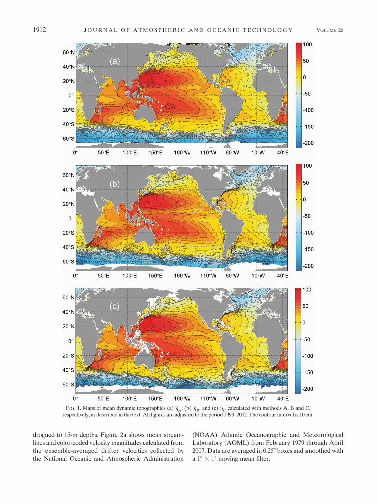
FIG. 1. Maps of mean dynamic topographies (a) hA, (b) hB, and (c) hC calculated with methods A, B and C,

respectively, as described in the text. All figures are adjusted to the period 1993–2002. The contour interval is 10 cm.


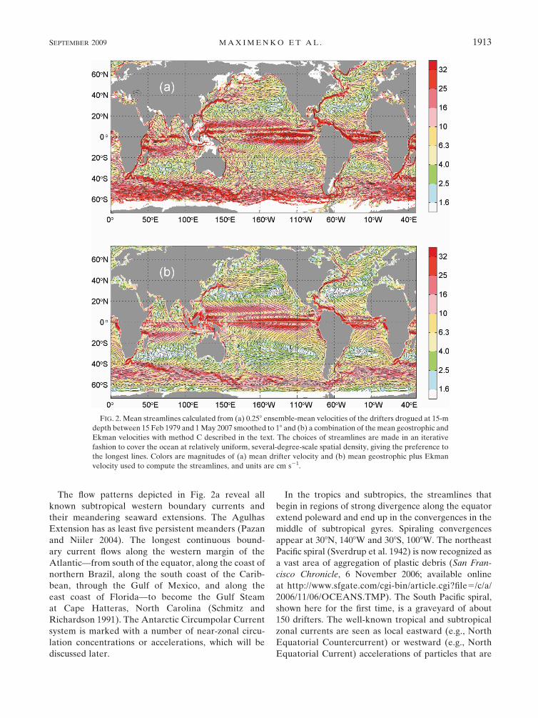
The flow patterns depicted in Fig. 2a reveal all

known subtropical western boundary currents and

their meandering seaward extensions. The Agulhas

Extension has as least five persistent meanders (Pazan

and Niiler 2004). The longest continuous bound-

ary current flows along the western margin of the

Atlantic—from south of the equator, along the coast of

northern Brazil, along the south coast of the Carib-

bean, through the Gulf of Mexico, and along the

east coast of Florida—to become the Gulf Steam

at Cape Hatteras, North Carolina (Schmitz and

Richardson 1991). The Antarctic Circumpolar Current

system is marked with a number of near-zonal circu-

lation concentrations or accelerations, which will be

discussed later.

In the tropics and subtropics, the streamlines that

begin in regions of strong divergence along the equator

extend poleward and end up in the convergences in the

middle of subtropical gyres. Spiraling convergences

appear at 308N, 1408W and 308S, 1008W. The northeast

Pacific spiral (Sverdrup et al. 1942) is now recognized as

a vast area of aggregation of plastic debris (San Fran-

cisco Chronicle, 6 November 2006; available online

at http://www.sfgate.com/cgi-bin/article.cgi?file5/c/a/

2006/11/06/OCEANS.TMP). The South Pacific spiral,

shown here for the first time, is a graveyard of about

150 drifters. The well-known tropical and subtropical

zonal currents are seen as local eastward (e.g., North

Equatorial Countercurrent) or westward (e.g., North

Equatorial Current) accelerations of particles that are

FIG. 2. Mean streamlines calculated from (a) 0.258 ensemble-mean velocities of the drifters drogued at 15-m

depth between 15 Feb 1979 and 1 May 2007 smoothed to 18 and (b) a combination of the mean geostrophic and

Ekman velocities with method C described in the text. The choices of streamlines are made in an iterative

fashion to cover the ocean at relatively uniform, several-degree-scale spatial density, giving the preference to

the longest lines. Colors are magnitudes of (a) mean drifter velocity and (b) mean geostrophic plus Ekman

velocity used to compute the streamlines, and units are cm s21.


generally flowing in the poleward direction from the

equator to converge in the centers of the subtropical

doldrums.

3. Ekman currents

To calculate h from the drifter data, first, wind-driven

Ekman currents must be isolated. In method B (Rio and

Hernandez 2003), parameterizations for monthly mean

Ekman velocities in 58 latitude bins were derived. These

parameterizations were used in this study with 6-hourly

European Centre for Medium-Range Weather Fore-

casts (ECMWF) reanalysis surface wind stress. Thus

obtained Ekman velocities were interpolated to drifter

locations and subtracted from the observed total drifter

velocities. Then, a 3-day low-pass filter was applied to

yield a geostrophic drifter velocity.

In method C (Maximenko and Niiler 2005), the right-

most terms in the momentum balance Eq. (1) are calcu-

lated from drifter and satellite data by regressing them

onto the vector winds according to

dV

dt1 k 3 f V 1 g$h9 1 g$h

A5 C � R(a) �W, (5)

where h9 is the Archiving, Validation and Interpretation

of Satellite Oceanographic data (Aviso) sea level anom-

aly (SLA; Ducet et al. 2000), hA

is the GRACE-based

MDT of method A (Tapley et al. 2004), R(a) is the ro-

tation matrix, and W is the 6-hourly, 10-m height NCEP

reanalysis wind (data available online at http://www.cdc.

noaa.gov/data/gridded/data.nmc.reanalysis.html). The

coefficient C and the rotation angle a are determined

from the 18 latitude band ensembles of the 6-hourly data

across the entire ocean basins, including the equator.

This model of the wind force, as expressed on the right-

hand side of Eq. (5), is used to compute the wind force

collocated with the drifter.

The computation of the Ekman velocity in method B is

biased toward periods between 3 and 20 days, and the

regression of the Ekman wind force in method C is biased

toward steady winds. In all cases, spatial scales of the

Ekman currents correspond to atmospheric scales and

generally are much larger than the oceanic mesoscale.

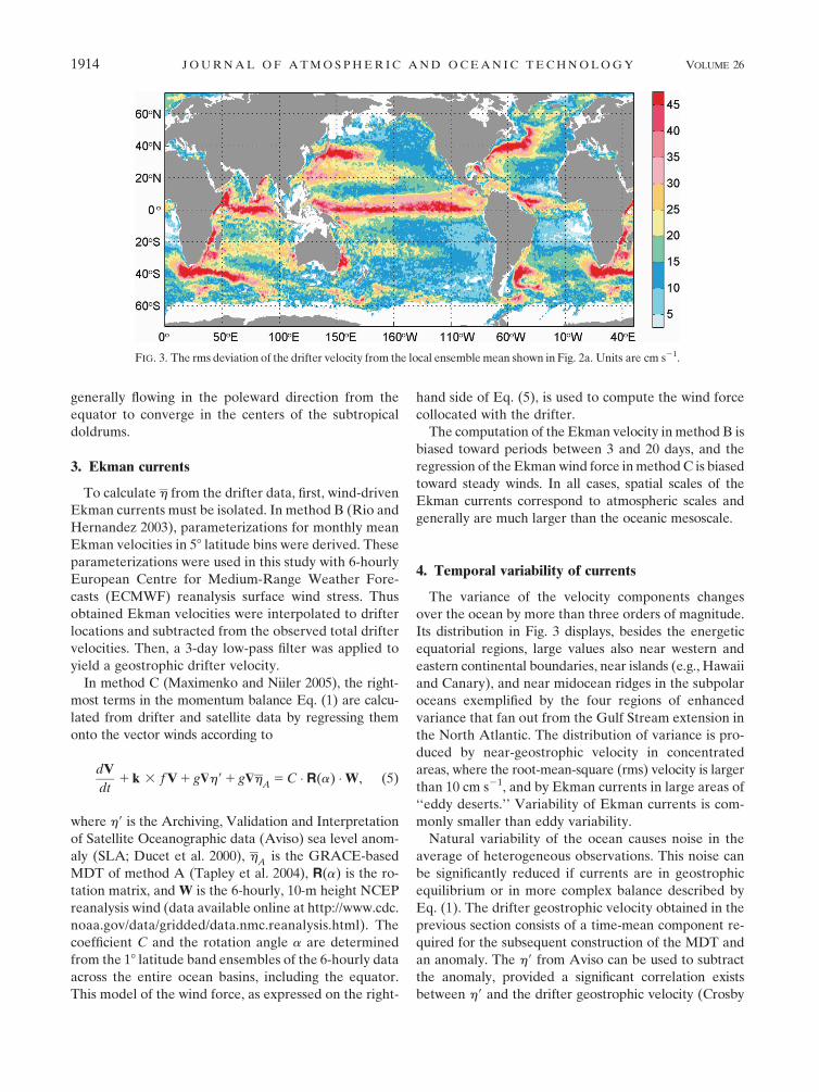
4. Temporal variability of currents

The variance of the velocity components changes

over the ocean by more than three orders of magnitude.

Its distribution in Fig. 3 displays, besides the energetic

equatorial regions, large values also near western and

eastern continental boundaries, near islands (e.g., Hawaii

and Canary), and near midocean ridges in the subpolar

oceans exemplified by the four regions of enhanced

variance that fan out from the Gulf Stream extension in

the North Atlantic. The distribution of variance is pro-

duced by near-geostrophic velocity in concentrated

areas, where the root-mean-square (rms) velocity is larger

than 10 cm s21, and by Ekman currents in large areas of

‘‘eddy deserts.’’ Variability of Ekman currents is com-

monly smaller than eddy variability.

Natural variability of the ocean causes noise in the

average of heterogeneous observations. This noise can

be significantly reduced if currents are in geostrophic

equilibrium or in more complex balance described by

Eq. (1). The drifter geostrophic velocity obtained in the

previous section consists of a time-mean component re-

quired for the subsequent construction of the MDT and

an anomaly. The h9 from Aviso can be used to subtract

the anomaly, provided a significant correlation exists

between h9 and the drifter geostrophic velocity (Crosby

FIG. 3. The rms deviation of the drifter velocity from the local ensemble mean shown in Fig. 2a. Units are cm s21.


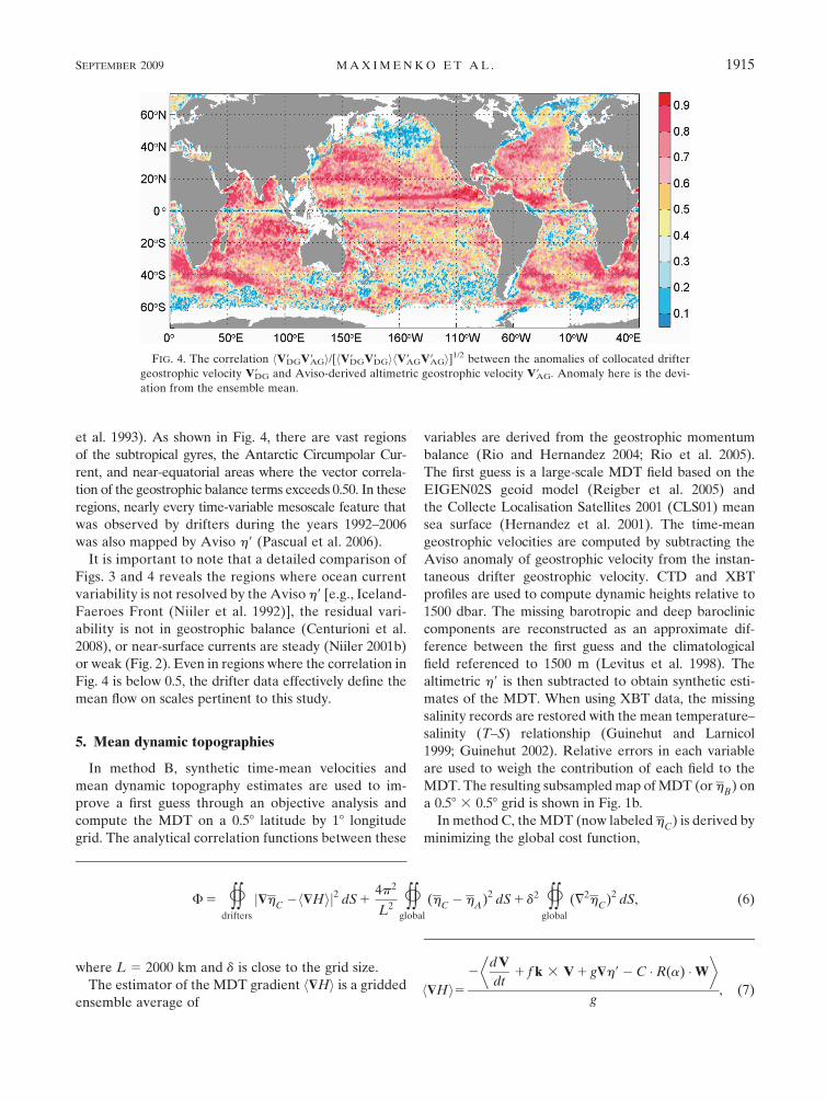
et al. 1993). As shown in Fig. 4, there are vast regions

of the subtropical gyres, the Antarctic Circumpolar Cur-

rent, and near-equatorial areas where the vector correla-

tion of the geostrophic balance terms exceeds 0.50. In these

regions, nearly every time-variable mesoscale feature that

was observed by drifters during the years 1992–2006

was also mapped by Aviso h9 (Pascual et al. 2006).

It is important to note that a detailed comparison of

Figs. 3 and 4 reveals the regions where ocean current

variability is not resolved by the Aviso h9 [e.g., Iceland-

Faeroes Front (Niiler et al. 1992)], the residual vari-

ability is not in geostrophic balance (Centurioni et al.

2008), or near-surface currents are steady (Niiler 2001b)

or weak (Fig. 2). Even in regions where the correlation in

Fig. 4 is below 0.5, the drifter data effectively define the

mean flow on scales pertinent to this study.

5. Mean dynamic topographies

In method B, synthetic time-mean velocities and

mean dynamic topography estimates are used to im-

prove a first guess through an objective analysis and

compute the MDT on a 0.58 latitude by 18 longitude

grid. The analytical correlation functions between these

variables are derived from the geostrophic momentum

balance (Rio and Hernandez 2004; Rio et al. 2005).

The first guess is a large-scale MDT field based on the

EIGEN02S geoid model (Reigber et al. 2005) and

the Collecte Localisation Satellites 2001 (CLS01) mean

sea surface (Hernandez et al. 2001). The time-mean

geostrophic velocities are computed by subtracting the

Aviso anomaly of geostrophic velocity from the instan-

taneous drifter geostrophic velocity. CTD and XBT

profiles are used to compute dynamic heights relative to

1500 dbar. The missing barotropic and deep baroclinic

components are reconstructed as an approximate dif-

ference between the first guess and the climatological

field referenced to 1500 m (Levitus et al. 1998). The

altimetric h9 is then subtracted to obtain synthetic esti-

mates of the MDT. When using XBT data, the missing

salinity records are restored with the mean temperature–

salinity (T–S) relationship (Guinehut and Larnicol

1999; Guinehut 2002). Relative errors in each variable

are used to weigh the contribution of each field to the

MDT. The resulting subsampled map of MDT (or hB) on

a 0.58 3 0.58 grid is shown in Fig. 1b.

In method C, the MDT (now labeled hC

) is derived by

minimizing the global cost function,

where L 5 2000 km and d is close to the grid size.

The estimator of the MDT gradient h$Hi is a gridded

ensemble average ofh$Hi5

2dV

dt1 f k 3 V 1 g$h9� C � R(a) �W

� �

g, (7)

FIG. 4. The correlation hV9DGV9AGi/[hV9DGV9DGihV9AGV9AGi]1/2 between the anomalies of collocated drifter

geostrophic velocity V9DG and Aviso-derived altimetric geostrophic velocity V9AG. Anomaly here is the devi-

ation from the ensemble mean.

F 5 6

drifters

j$hC�h$Hij2 dS 1

4p2

L26

global

(hC� h

A)2 dS 1 d2

6

global

(=2hC

)2 dS, (6)


which is calculated from the 6-hourly collocated data of

drifters, SLA, and wind. The map of hC

is presented in

Fig. 1c (data are available online at http://apdrc.soest.

hawaii.edu/projects/DOT). It can be shown (Maximenko

and Niiler 2005) that, on scales larger than L, hC is

strongly controlled by hA, whereas on smaller scales

it is mostly defined by the drifter-derived velocity.

Laplacian smoothing is added to reduce the grid noise. If

not blended with hA

[the second term in the right-hand

side of Eq. (6)], hC

closely follows the mean dynamic

topography of Niiler et al. (2003), which tends to slightly

overestimate the sea level difference across the main

large-scale gyres and Antarctic Circumpolar Current.

The MDTs hB and hC—derived with methods B

and C, respectively—produce remarkably consistent pic-

tures, with a global rms difference of 6.5 cm. The largest

difference is south of 558S; if this area is excluded, then

a 4.1-cm rms difference results. Methods B and C can be

viewed as adding small-scale signal to hA

. This does not

change the pattern of large-scale geostrophic circulation

(cf. Figs. 1a,c), and the rms difference between hC and hA

is 7.3 cm, which is small compared to the range of hC.

Yet, this difference is concentrated at small scales and

produces differences in spatial gradients and corre-

sponding geostrophic velocities. The rms velocities de-

rived from hC

and hA

outside the 58 equatorial band are

8.9 and 6.9 cm s21, respectively. The rms of the difference

between the two velocities is 6.7 cm s21. For comparison,

hB yields the rms velocity of 8.5 cm s21, while the rms

difference between the hB- and hC-produced velocities is

4.2 cm s21. The denser concentration of sea level isolines

in Figs. 1b,c highlights the fact that practically all current

systems are sharper and faster than one would deduct

from Fig. 1a. The difference between hA

and hC

(or hB

)

is particularly evident in geostrophic velocities shown in

Fig. 5. Although the velocities calculated from hA are

broader and weaker than the ones from hB and hC, in-

herent spatial noise contributes significantly to obscuring

the difference in the energy levels of the currents esti-

mated above.

Equation (2) suggests that a mean velocity can be

constructed by adding Ekman and geostrophic veloci-

ties. Figure 2b shows the map of such a circulation

pattern calculated from hC and C, R(a), and NCEP

10-m winds averaged over the period of 1993–2002. The

correspondence between Figs. 2a,b is quite remarkable,

thus demonstrating the validity of Eq. (2). The largest

difference between the total and the geostrophic near-

surface flow paths (Fig. 1c) is attained in the tropics where

the mean streamlines move away from the equator while

the geostrophic streamlines move toward the equator.

Generally, the mesoscale features, discernible in both

Figs. 1b,c, appear in all oceans and are nearly identical.

To a large extent, this is due to the direct observations of

velocity with drifters used in both methods described in

this paper. Moving eastward with the steady meandering

pattern of the Agulhas Current extension off the tip of

the South Africa (Ochoa and Niiler 2007), at least eight

regions of highly concentrated, or accelerated, eastward

flows of the Antarctic Circumpolar Current system can

be identified in both Figs. 1 and 2. These flow features

are real, because their near-surface vorticity balance

can be understood combining the dynamics of standing

Rossby waves and their interaction with the underlying

topographic features (Hughes 2005).

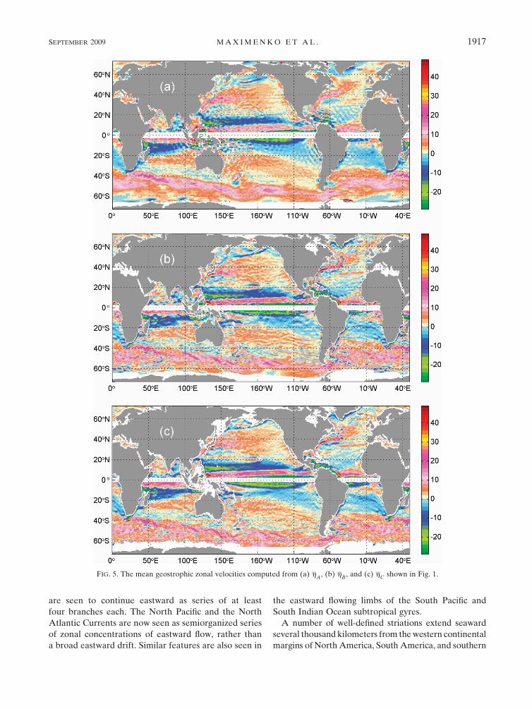
6. New features on the map of ocean circulation

The zonal geostrophic mean velocities computed

from hA

, hB

, and hC

were selectively colored in Fig. 5

to enhance values between 1 and 10 cm s21. This high-

lights many small-scale features that are embedded in

the broader flows. Each of the features can be traced

back to drifter velocities, where, however, they are not

as well defined because of the eddy noise and Ekman

currents. The pattern of the near-surface geostrophic

velocity is also interesting because it is expected to

have subsurface extension, perhaps, well into the ocean

thermocline.

In the North Pacific and North Atlantic, south of the

seaward extensions of the western boundary current are

westward flows, or the southern limbs of the Kuroshio

Extension and Gulf Stream recirculations. In both oceans,

a pattern of alternating striations continues southward. In

the North Atlantic, the eastward striation at approxi-

mately 358N is the Azores Current (Juliano and Alves

2007), now for the first time seen to be extending

westward to the longitude of Bermuda at 728W. North

of it in Fig. 5c is a coherent eastward striation, hereto-

fore not described, that connects the Mann Eddy (Mann

1967) to the coast of Portugal along 408N. A clockwise

flow is visible around the Reykjanes Ridge at 608N as

are the Iceland-Faeroes Islands Front and the Norwe-

gian Current farther to the north and east.

In the western North Pacific, the eastward stria-

tion at approximately 228N is known as the Subtropical

Countercurrent (Uda and Hasunuma 1969), but the

westward striation north of it has not been described

before. North of the Hawaiian Islands at 24.58N is an

eastward striation that was observed with expendable

velocity probes in 1985 (Niiler et al. 1991) to extend well

below the main thermocline, but its persistence was not

realized until now. The pair of alternating striations

in Figs. 5b,c west of the Hawaiian Islands is known

as the Hawaiian Lee Countercurrent (Xie et al. 2001).

The Kuroshio Extension and the Gulf Stream extension


are seen to continue eastward as series of at least

four branches each. The North Pacific and the North

Atlantic Currents are now seen as semiorganized series

of zonal concentrations of eastward flow, rather than

a broad eastward drift. Similar features are also seen in

the eastward flowing limbs of the South Pacific and

South Indian Ocean subtropical gyres.

A number of well-defined striations extend seaward

several thousand kilometers from the western continental

margins of North America, South America, and southern

FIG. 5. The mean geostrophic zonal velocities computed from (a) hA, (b) hB, and (c) hC shown in Fig. 1.


Africa. Along the California coast, these have roots in the

permanent meanders of the California Current System,

which appear to be caused by the seaward influence of its

semipermanent meanders (Centurioni et al. 2008). Off

the California coast, as well as off the coast of Chile, the

depth structure of these near-zonal flows appears also in

historical hydrographic data (Maximenko et al. 2008).

The depth structure of the strong eastward St. Helena

Current, which approaches the tip of South Africa from

the west, also appears in historical files (Juliano and

Alves 2007). Figure 5 presents a new context in which to

view the continued datasets from satellites and drifters.

Results of the Gravity Field and Steady-State Ocean

Circulation Explorer (GOCE) mission (available online

at http://www.esa.int/esaLP/LPgoce.html) are anticipated

to further improve the gravity model, and observations

currently being made by over 3000 Argo profiling floats

(available online at http://www.argo.ucsd.edu) will ex-

tend the refined pattern of the mean circulation into the

interior of the ocean.

Acknowledgments. This work was supported by the

NASA Ocean Surface Topography Science Team and

NASA GRACE Science Team. N.M. and O.M. were

also supported by NSF Grant OCE05-50853, the Japan

Agency for Marine-Earth Science and Technology

(JAMSTEC), NASA through Grant NNX07AG53G,

and NOAA through Grant NA17RJ1230. NASA and

NOAA sponsor research at the International Pacific

Research Center. B.G. was partly supported by ARO

Grant W911NF-05-1-0055 and ONR Grant N00014-07-1-

1065. Satellite altimetry data were acquired from the

Aviso and drifter data from the NOAA AOML. Help of

Dr. Yoo-Yin Kim is gratefully acknowledged.

REFERENCES

Centurioni, L. R., J. C. Ohlmann, and P. P. Niiler, 2008: Permanent

meanders in the California Current System. J. Phys. Ocean-

ogr., 38, 1690–1710.

Crosby, D. S., L. C. Breaker, and W. H. Gemmill, 1993: A pro-

posed definition for vector correlation in geophysics: Theory

and application. J. Atmos. Oceanic Technol., 10, 355–367.

Ducet, N., P. Y. LeTraon, and G. Reverdin, 2000: Global high-

resolution mapping of ocean circulation from TOPEX/

Poseidon and ERS-1 and -2. J. Geophys. Res., 105 (C8),

19 477–19 489.

Gill, A. E., 1982: Atmosphere–Ocean Dynamics. Academic Press,

662 pp.

Guinehut, S., 2002: Vers une utilisation combinee des donnees

altimetriques et des mesures des flotteurs profilants. Ph.D.

thesis, Universite Paul Sabatier, 168 pp.

——, and G. Larnicol, 1999: Impact de la salinite dans le calcul des

hauteurs dynamiques—Etude effectuee a partir des sections

WOCE de l’ocean Atlantique. Collecte Localisation Satellites

Contract CNES/CLS 794/98/CNES/7235, 27 pp.

Hernandez, F., P. Schaeffer, M.-H. Calvez, J. Dorandeu, Y. Faugere,

and F. Mertz, 2001: Surface Moyenne Oceanique: Support

Scientifique a la mission altimetrique Jason-1, et a une mission

micro-satellite altimetrique. Collecte Localisation Satellites

Final Rep. CLS/DOS/NT/00.341, 150 pp.

Hughes, C. W., 2005: Nonlinear vorticity balance of the Antarc-

tic Circumpolar Current. J. Geophys. Res., 110, C11008,

doi:10.1029/2004JC002753.

Imawaki, S., H. Uchida, H. Ichikawa, M. Fukasawa, and S. Umatani,

ASUKA Group, 2001: Satellite altimeter monitoring the Kur-

oshio Transport south of Japan. Geophys. Res. Lett., 28, 17–20.

Juliano, M. F., and M. L. G. R. Alves, 2007: The Atlantic sub-

tropical front/current systems of Azores and St. Helena.

J. Phys. Oceanogr., 37, 2573–2598.

Large, W. G., 1998: Modeling and parameterizing the ocean plane-

tary boundary layer. Ocean Modeling and Parameterization. E.

P. Chassignet and J. Verron, J., Eds., Kluwer Academic, 81–120.

Levitus, S., and Coauthors, 1998: Introduction. Vol. 1, World

Ocean Database 1998. NOAA Atlas NESDIS 18, 346 pp.

Mann, C. R., 1967: The termination of the Gulf Stream and the

beginning of the North Atlantic Current. Deep-Sea Res., 14,

337–359.

Maximenko, N. A., and P. P. Niiler, 2005: Hybrid decade-mean

global sea level with mesoscale resolution. Recent Advances

in Marine Science and Technology, 2004, N. Saxena, Ed.,

PACON International, 55–59.

——, and ——, 2008: Tracking ocean debris. IPRC Climate, Vol. 8,

No. 2, International Pacific Research Center, 14–16. [Available

online at http://iprc.soest.hawaii.edu/publications/newsletters/

newsletter_sections/iprc_climate_vol8_2/tracking_ocean_debris.

pdf.]

——, O. V. Melnichenko, P. P. Niiler, and H. Sasaki, 2008: Sta-

tionary mesoscale jet-like features in the ocean. Geophys. Res.

Lett., 35, L08603, doi:10.1029/2008GL033267.

Nerem, R. S., B. D. Tapley, and C. K. Shum, 1990: Determina-

tion of the ocean general circulation using Geosat altimetry.

J. Geophys. Res., 95 (C3), 3163–3179.

Niiler, P. P., 2001a: The world ocean surface circulation. Ocean

Circulation and Climate, G. Siedler, J. Church, and J. Gould,

Eds., Academic Press, 193–204.

——, 2001b: Global ocean circulation observations. Observing the

Oceans in the 21st Century, C. J. Koblinsky and N. R. Smith,

Eds., Australian Bureau of Meteorology, 306–323.

——, D. K. Lee, W. Young, and L. H. Hu, 1991: Expendable

current profiler (XCP) section across the North Pacific at

258N. Deep-Sea Res., 38, S45–S61.

——, S. Piacsek, L. Neuberg, and A. Warn-Varnas, 1992: Scales of

SST variability of the Iceland-Faeroe Front. J. Geophys. Res.,

97 (C11), 17 777–17 785.

——, N. A. Maximenko, and J. C. McWilliams, 2003: Dynamically

balanced absolute sea level of the global ocean derived from

near-surface velocity observations. Geophys. Res. Lett., 30,

2164, doi:10.1029/2003GL018628.

Ochoa, J., and P. P. Niiler, 2007: Vertical vorticity balance in

meanders downstream the Agulhas retroflection. J. Phys.

Oceanogr., 37, 740–744.

Pascual, A., Y. Faugere, G. Larnicol, and P.-Y. Le Traon, 2006:

Improved description of the ocean mesoscale variability by

combining four satellite altimeters. Geophys. Res. Lett., 33,

L02611, doi:10.1029/2005GL024633.

Pazan, S. E., and P. Niiler, 2004: New global drifter data set

available. Eos, Trans. Amer. Geophys. Union, 85, doi:10.1029/

2004EO020007.


Ralph, E. A., K. Bi, P. P. Niiler, and Y. A. du Penhoat, 1997: A

Lagrangian description of the western equatorial Pacific re-

sponse to the wind burst of December 1992: Heat advection in

the warm pool. J. Climate, 10, 1706–1721.

Reigber, C., R. Schmidt, F. Flechtner, R. Konig, U. Meyer, K.-H.

Neumayer, P. Schwintzer, and S. Y. Zhu, 2005: An Earth

gravity field model complete to degree and order 150 from

GRACE: EIGEN-GRACE02S. J. Geodyn., 39, 1–10.

Reverdin, G., P. P. Niiler, and H. Valdimarsson, 2003: North Atlantic

Ocean surface currents. J. Geophys. Res., 108 (C1), 3002–3004.

Richardson, P. L., 1989: Worldwide ship drift distributions identify

missing data. J. Geophys. Res., 94, 6169–6176.

Rio, M.-H., and F. Hernandez, 2003: High-frequency response

of wind-driven currents measured by drifting buoys and

altimetry over the world ocean. J. Geophys. Res., 108, 3283,

doi:10.1029/2002JC001655.

——, and ——, 2004: A mean dynamic topography computed over

the world ocean from altimetry, in situ measurements, and a

geoid model. J. Geophys. Res., 109, C12032, doi:10.1029/

2003JC002226.

——, P. Schaeffer, and J. M. Lemoine, 2005: The estimation of the

ocean mean dynamic topography through the combination of

altimetric data, in-situ measurements and GRACE geoid:

From global to regional studies. Proc. GOCINA Int. work-

shop, Luxembourg, Centre Europeen de Geodynamique et de

Seismologie.

Robinson, A. R., Ed., 1983: Eddies in Marine Science. Springer-

Verlag, 609 pp.

Rudnick, D. L., 1996: Intensive surveys of the Azores Front 2.

Inferring the geostrophic and vertical velocity fields. J. Geo-

phys. Res., 101, 16 291–16 303.

Schmitz, W. J., and P. L. Richardson, 1991: On the sources of the

Florida Current. Deep-Sea Res., 38 (Suppl.), 389–409.

Siedler, G., J. Church, and J. Gould, Eds., 2001: Ocean Circulation

and Climate. Academic Press, 715 pp.

Stammer, D., 1997: Global characteristics of ocean variability es-

timated from regional TOPEX/Poseidon altimeter measure-

ments. J. Phys. Oceanogr., 27, 1743–1769.

Sverdrup, H. U., M. W. Johnson, and R. H. Flemming, 1942: The

Oceans: Their Physics, Chemistry, and General Biology.

Prentice-Hall, 1087 pp.

Tapley, B. D., D. P. Chambers, S. Bettadpur, and J. C. Ries, 2003:

Large scale ocean circulation from the GRACE GGM01 Ge-

oid. Geophys. Res. Lett., 30, 2163, doi:10.1029/2003GL018622.

——, S. Bettadpur, M. Watkins, and C. Reigber, 2004: The Gravity

Recovery and Climate Experiment: Mission overview and

early results. Geophys. Res. Lett., 31, L09607, doi:10.1029/

2004GL019920.

Uchida, H., and S. Imawaki, 2003: Eulerian mean surface velocity

field derived by combining drifter and satellite altimeter data.

Geophys. Res. Lett., 30, 1229, doi:10.1029/2002GL016445.

——, ——, and J.-H. Hu, 1998: Comparison of Kuroshio surface

velocities derived from satellite altimeter and drifting buoy

data. J. Oceanogr., 54, 115–122.

Uda, M., and K. Hasunuma, 1969: The eastward subtropical

countercurrent in the western North Pacific Ocean. J. Ocean-

ogr. Soc. Japan, 25, 201–210.

Wunsch, C., and E. M. Gaposchkin, 1980: On using satellite al-

timetry to determine the general circulation of the oceans, with

application to geoid improvement. Rev. Geophys., 18, 725–745.

Xie, S.-P., W. T. Liu, Q. Liu, and M. Nonaka, 2001: Far-reaching

effect of the Hawaiian Islands on the Pacific Ocean-atmosphere

system. Science, 292, 2057–2060.

Zlotnicki, V., and J. G. Marsh, 1989: Altimetry, ship gravimetry,

and the general circulation of the North Atlantic. Geophys.

Res. Lett., 16, 1011–1014.


mean dynamic topography of the ocean derived from...

Documents