me964 high performance computing for engineering...
TRANSCRIPT
ME964High Performance Computing for Engineering Applications
“The real problem is not whether machines think but whether men do.”
B. F. Skinner© Dan Negrut, 2011ME964 UW-Madison
Outlining Midterm ProjectsTopic 3: GPU-based FEA
Topic 4: GPU Direct Solver for Sparse Linear Algebra
March 01, 2011

Before We Get Started…
Last time
Midterm Project topics 1 and 2
Discrete Element Method on the GPU. Area coordinator: Toby Heyn
Collision Detection on the GPU. Area coordinator: Arman Pazouki
Today
Midterm Project topics 3 and 4
Finite Element Method on the GPU. Area coordinators: Prof. Suresh and Naresh Khude
Sparse direct solver on the GPU (Cholesky). Area coordinator: Dan Negrut
Midterm Project Related Issues Midterm Project is due on 04/13 at 11:59 PM (use Learn@UW drop-box)
Intermediate report due on 03/22 at 11:59 PM (use the same Learn@UW drop-box)
Each area coordinator Will provide a test problem for you to test your GPU implementation
Will also assist you with questions related to the non-programming aspects (the “theory”) behind the topic you chose
You can continue your Midterm Project (MP) and have it become your Final Project (FP) In this case you will be expected to show how the FP implementation is superior to your MP implementation
Other issues
HW5 due tonight at 11:59 PM
Use Learn@UW drop-box to submit homework 2
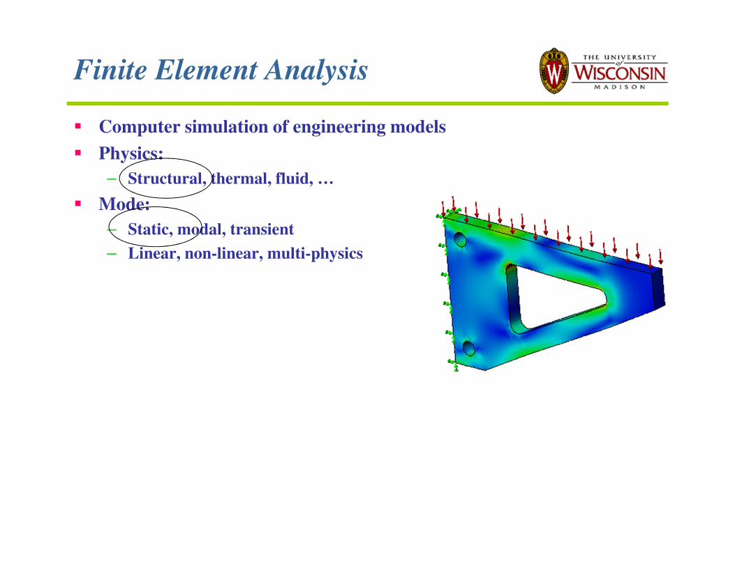
Finite Element Analysis
Computer simulation of engineering models
Physics:
– Structural, thermal, fluid, …
Mode:
– Static, modal, transient
– Linear, non-linear, multi-physics
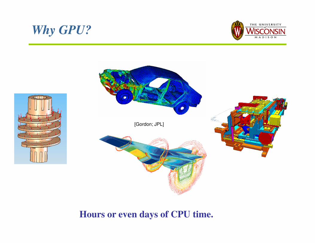
Why GPU?
Hours or even days of CPU time.
[Gordon; JPL]
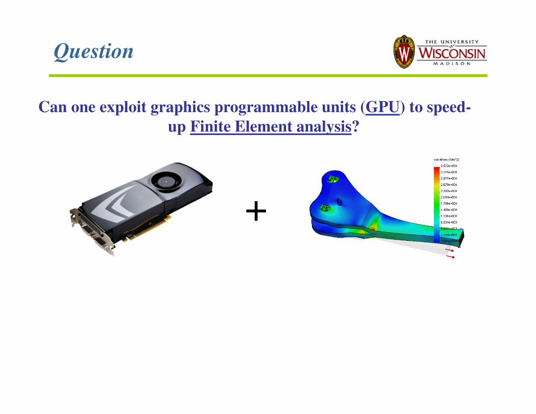
Question
Can one exploit graphics programmable units (GPU) to speed-
up Finite Element analysis?
+
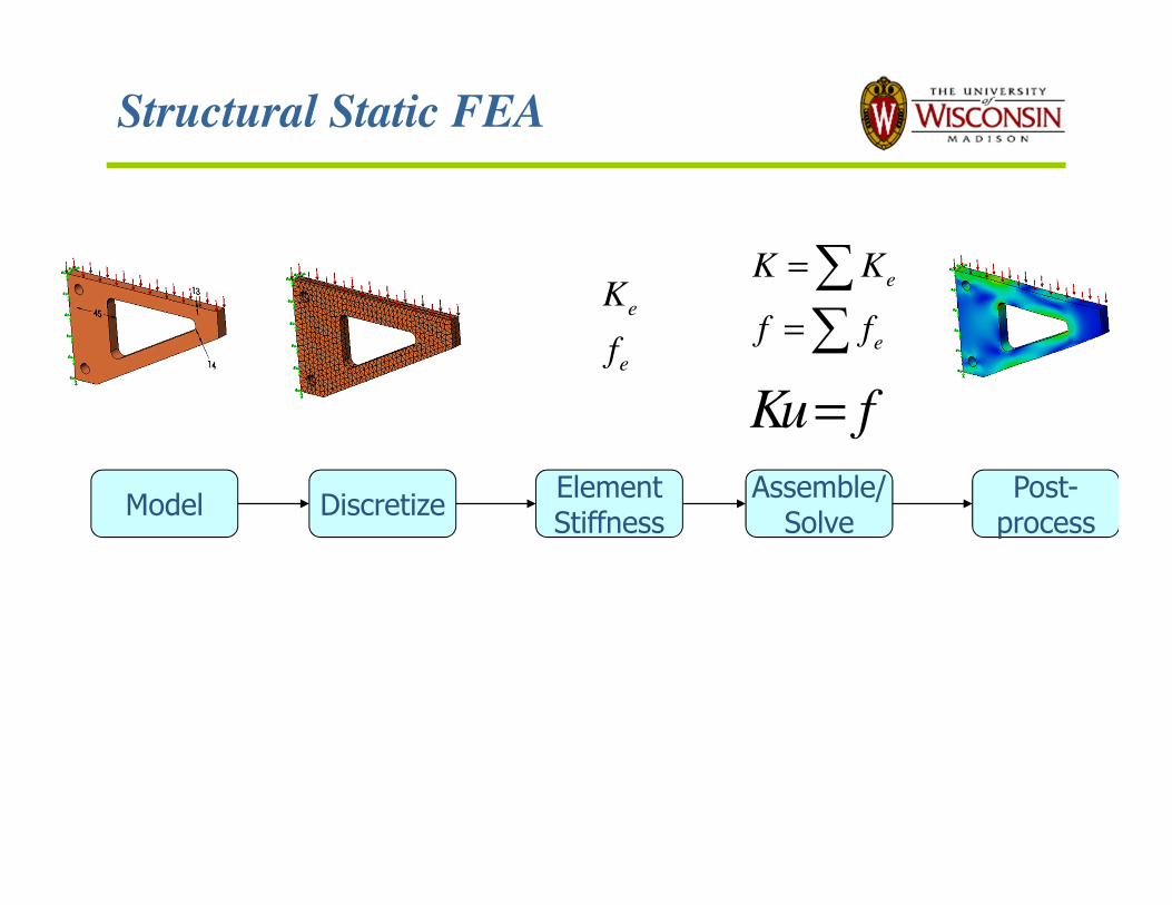
Structural Static FEA
Model DiscretizePost-
processElementStiffness
e
e
K
f
Assemble/Solve
Ku f=
e
e
K K
f f
=
=
∑∑
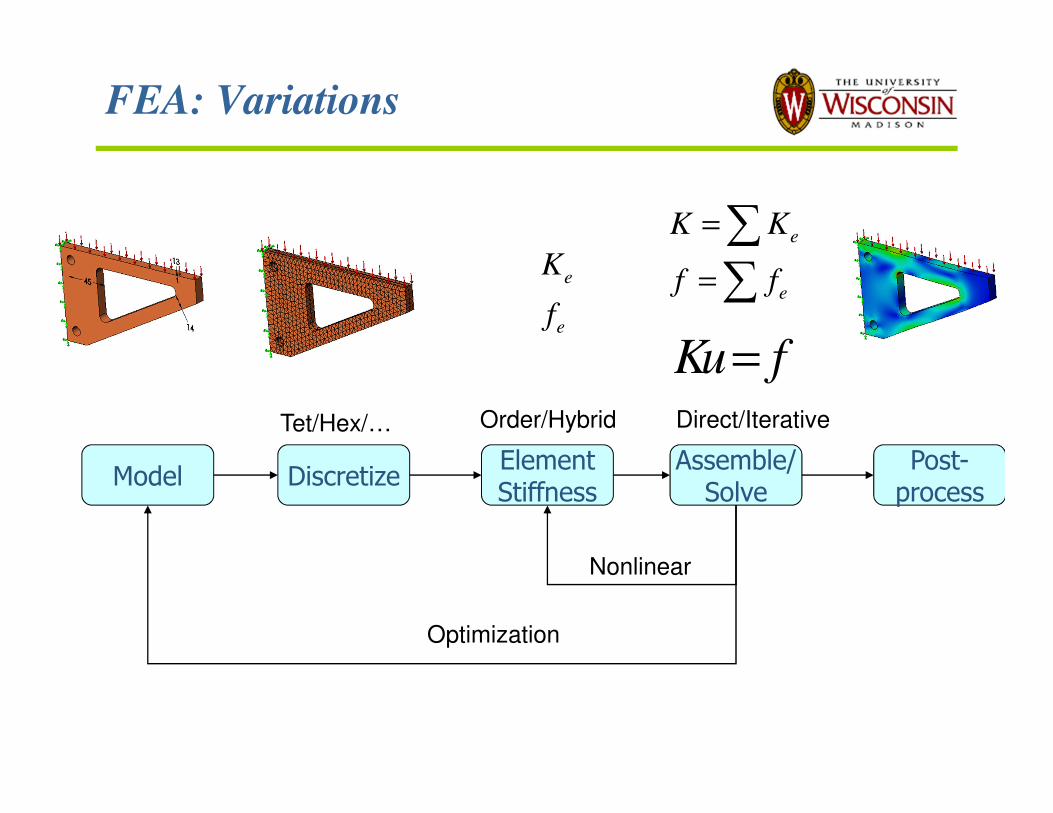
FEA: Variations
DiscretizeModelElementStiffness
Assemble/Solve
Post-process
e
e
K K
f f
=
=
∑∑
Ku f=
Nonlinear
Optimization
Tet/Hex/… Direct/IterativeOrder/Hybrid
e
e
K
f
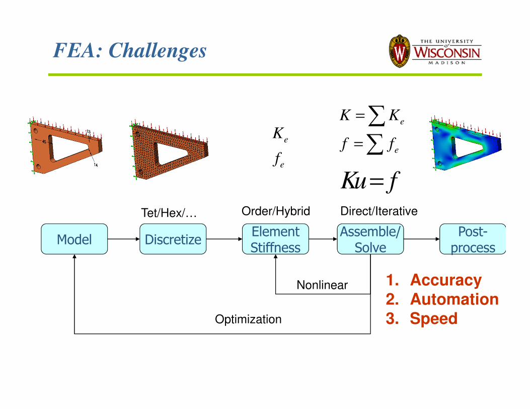
FEA: Challenges
DiscretizeModelElementStiffness
Assemble/Solve
Post-process
e
e
K K
f f
=
=
∑∑
Ku f=
Nonlinear
Optimization
Tet/Hex/… Direct/IterativeOrder/Hybrid
e
e
K
f
1. Accuracy2. Automation3. Speed
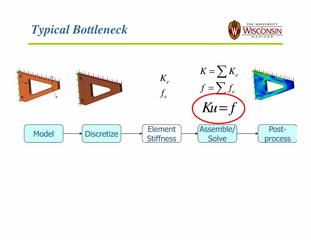
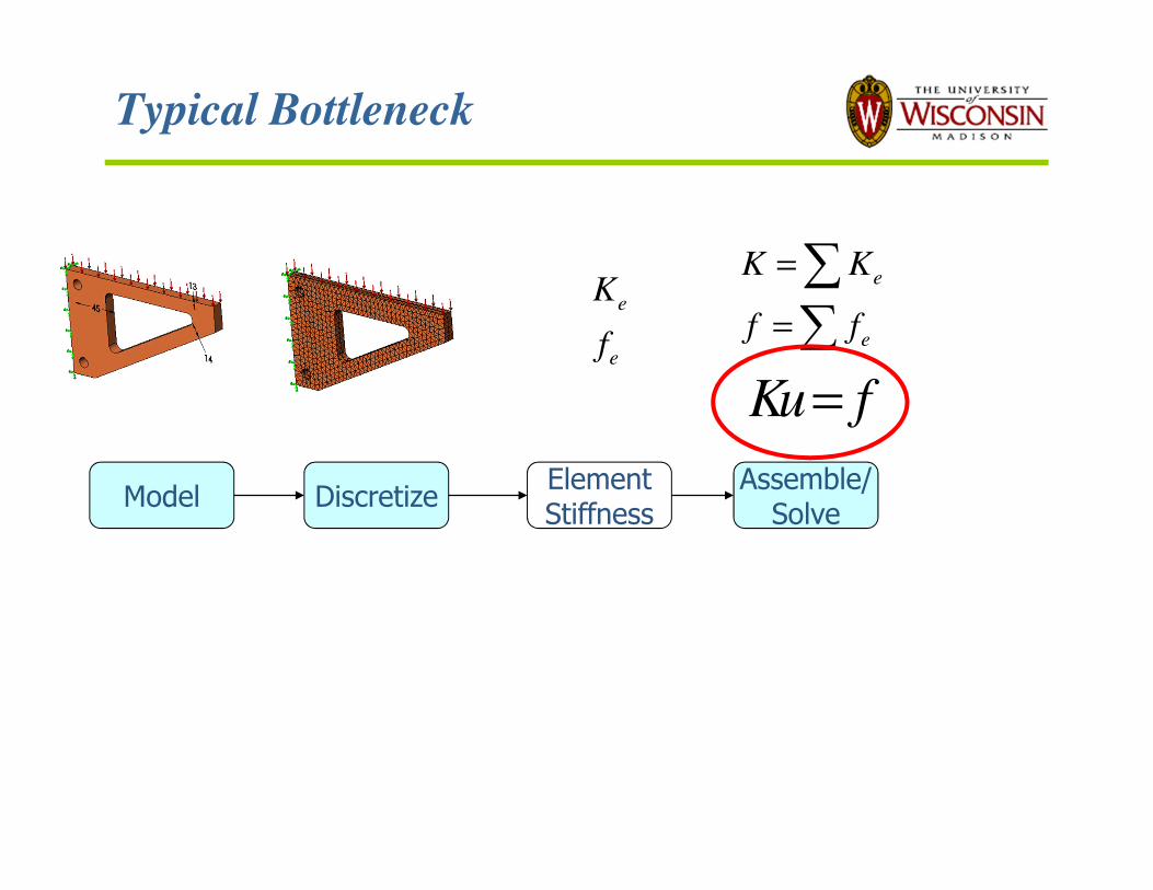
Typical Bottleneck
Model DiscretizePost-
processElementStiffness
e
e
K
f
Assemble/Solve
Ku f=
e
e
K K
f f
=
=
∑∑
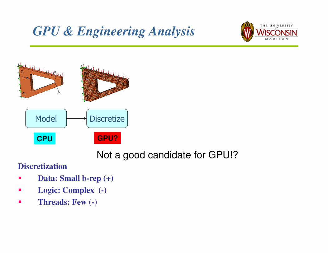
GPU & Engineering Analysis
Model Discretize
CPU GPU?
Discretization
Data: Small b-rep (+)
Logic: Complex (-)
Threads: Few (-)
Not a good candidate for GPU!?
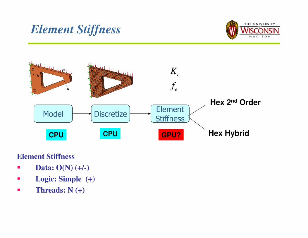
Element Stiffness
Element Stiffness
Data: O(N) (+/-)
Logic: Simple (+)
Threads: N (+)
DiscretizeModelElementStiffness
e
e
K
f
CPU CPU GPU?
Hex 2nd Order
Hex Hybrid
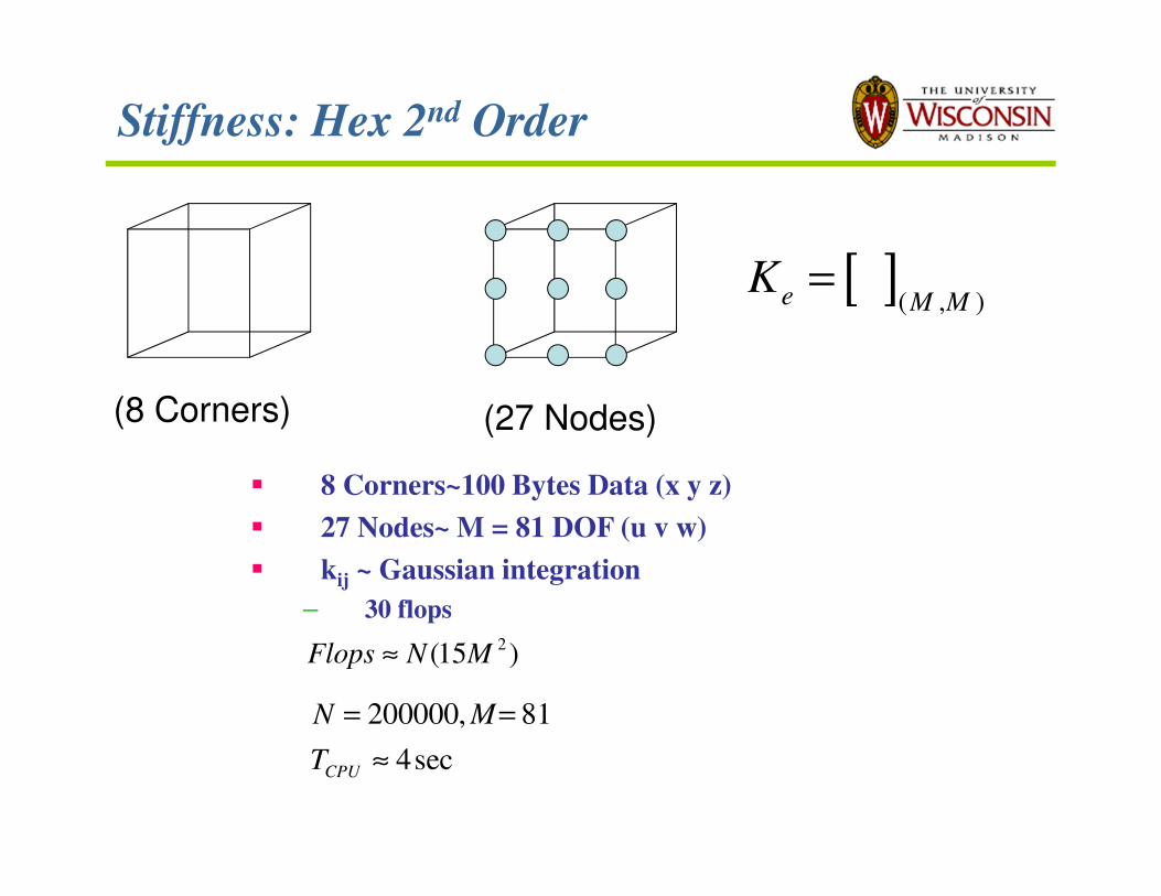
Stiffness: Hex 2nd Order
[ ]( , )e M M
K =
8 Corners~100 Bytes Data (x y z)
27 Nodes~ M = 81 DOF (u v w)
kij ~ Gaussian integration
– 30 flops
(8 Corners) (27 Nodes)
2(15 )Flops N M≈
200000, 81
4secCPU
N M
T
= =
≈
Typical Bottleneck
Model DiscretizeElementStiffness
e
e
K
f
Assemble/Solve
Ku f=
e
e
K K
f f
=
=
∑∑
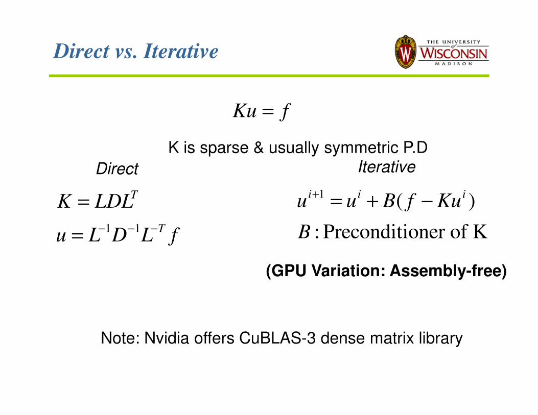
Direct vs. Iterative
Ku f=
K is sparse & usually symmetric P.D
1 1
T
T
K LDL
u L D L f− − −
=
=
Direct
1 ( )
: Preconditioner of K
i i iu u B f Ku
B
+ = + −
Iterative
(GPU Variation: Assembly-free)
Note: Nvidia offers CuBLAS-3 dense matrix library
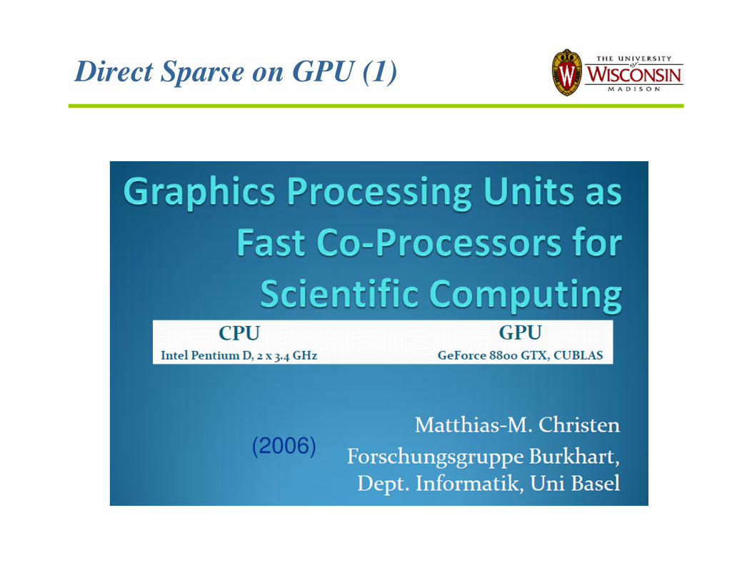
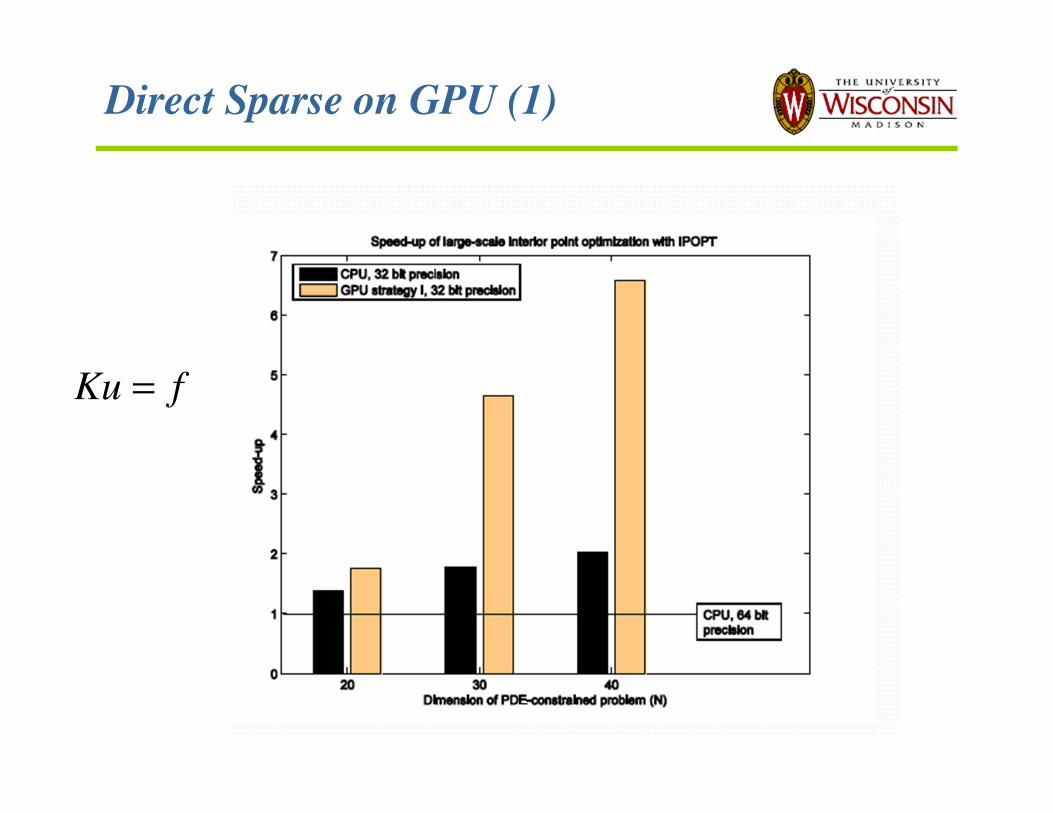
Direct Sparse on GPU (1)
(2006)
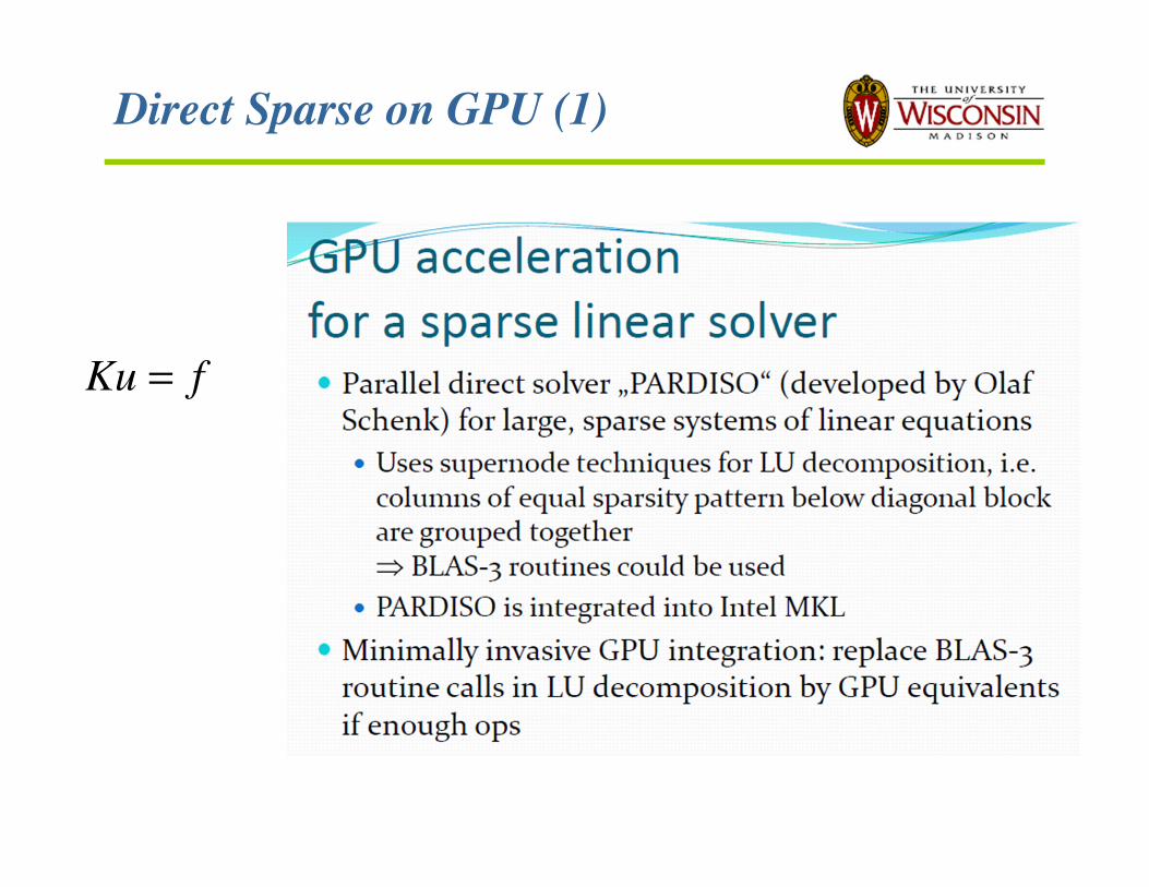
Direct Sparse on GPU (1)
Ku f=
Direct Sparse on GPU (1)
Ku f=
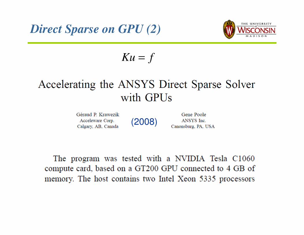
Direct Sparse on GPU (2)
Ku f=
(2008)
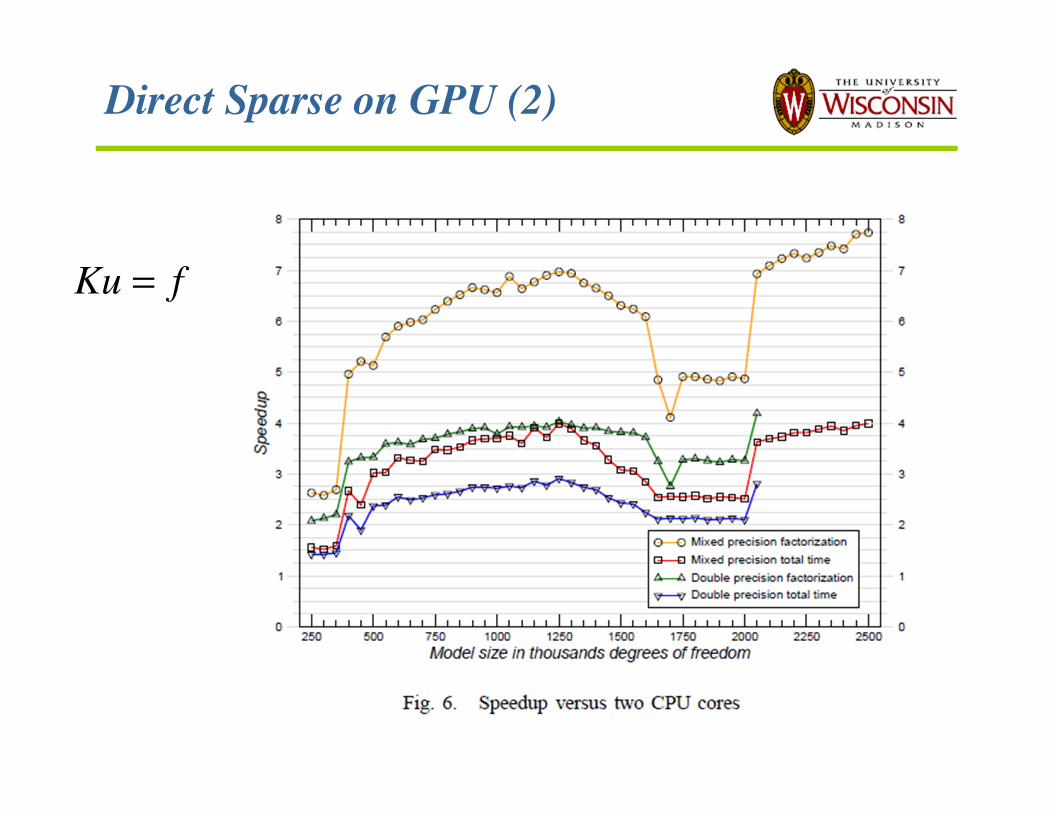
Direct Sparse on GPU (2)
Ku f=
Iterative Sparse on GPU (1)
(2008)
Jacobi preconditioned conjugate gradient
ATI GPU
Speed-up 3.5.
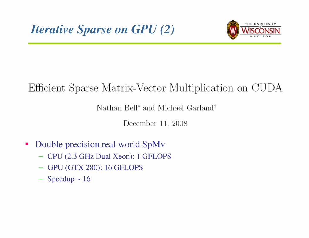
Iterative Sparse on GPU (2)
Double precision real world SpMv
– CPU (2.3 GHz Dual Xeon): 1 GFLOPS
– GPU (GTX 280): 16 GFLOPS
– Speedup ~ 16
FEA/GPU Class Projects?
1. Complete < 6 weeks
2. Important (publishable)
3. Pilot code
FEA/GPU Class Projects?
1. GPU Friendly Preconditioners for Thin Structures
– Research papers
– OpenCL and ViennaCL Pilot Code
2. Topology Optimization
– Research papers
– CUDA code
3. Others
– Can discuss …
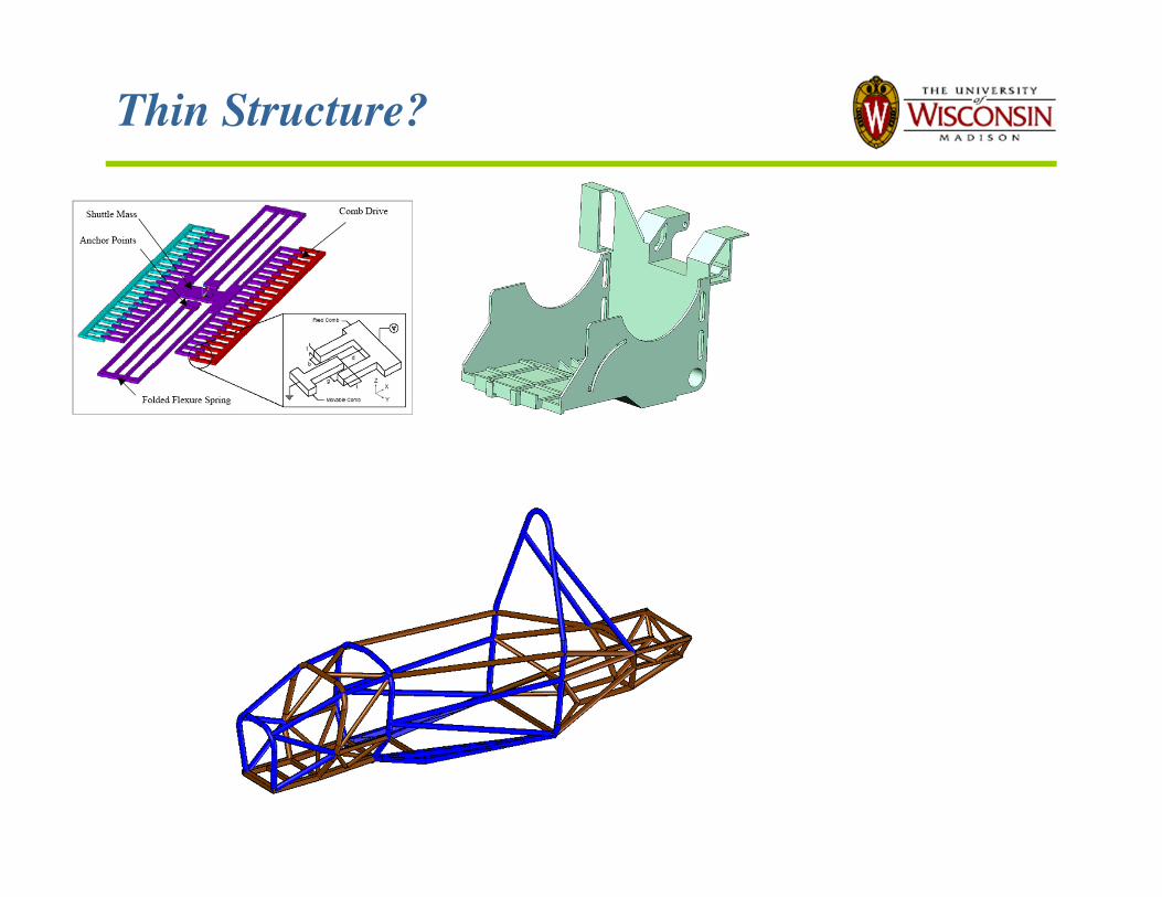
Thin Structure?
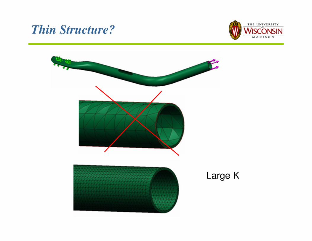
Thin Structure?
Large K
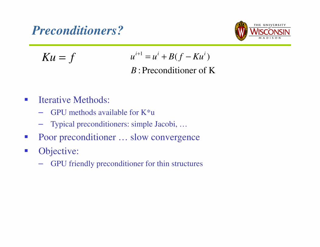
Preconditioners?
Ku f=
Iterative Methods:
– GPU methods available for K*u
– Typical preconditioners: simple Jacobi, …
Poor preconditioner … slow convergence
Objective:
– GPU friendly preconditioner for thin structures
1 ( )
: Preconditioner of K
i i iu u B f Ku
B
+ = + −
Research Publication
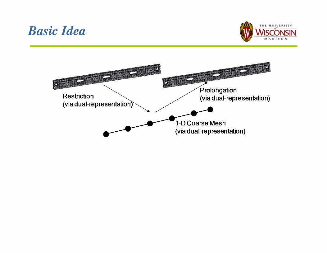
Basic Idea
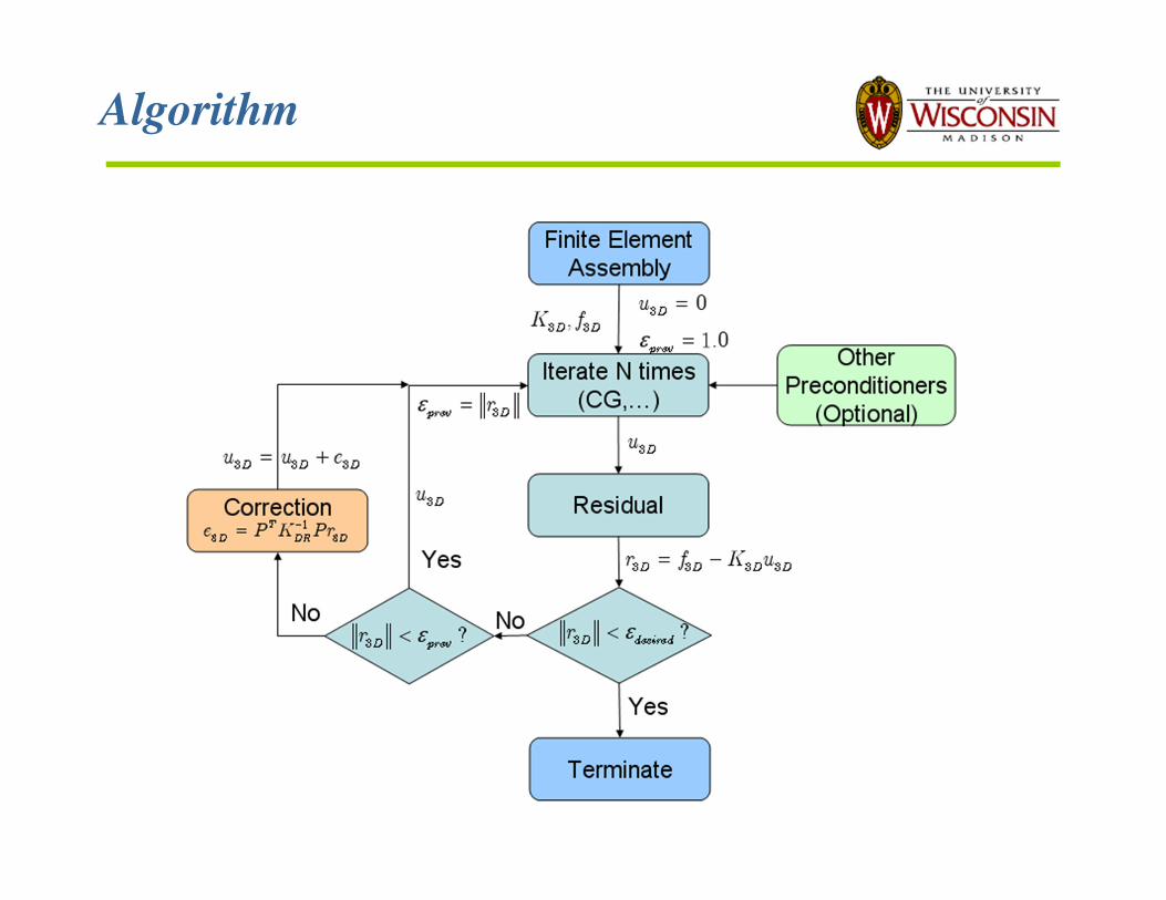
Algorithm
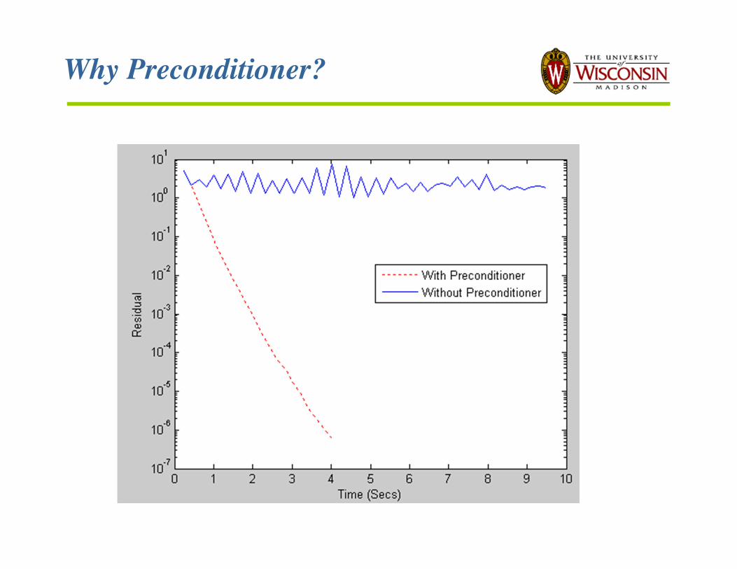
Why Preconditioner?
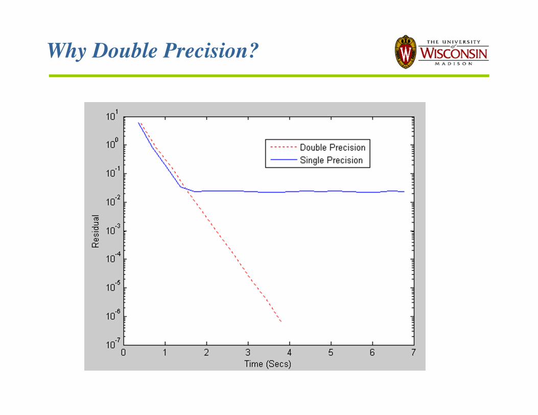
Why Double Precision?
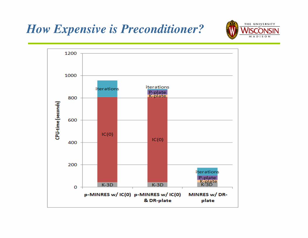
How Expensive is Preconditioner?
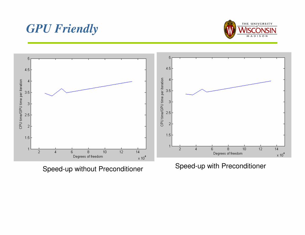
GPU Friendly
Speed-up without Preconditioner Speed-up with Preconditioner

FEA/GPU Class Projects?
1. GPU Friendly Preconditioners for Thin Structures
– Research papers
– OpenCL and ViennaCL Pilot Code
2. Topology Optimization
– Research papers
– CUDA code
3. Others
– Can discuss …
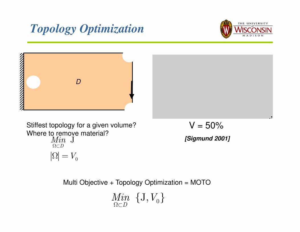
Topology Optimization
0
JD
Min
V
Ω⊂
Ω =
0 J, D
Min VΩ⊂
D
[Sigmund 2001]
V = 50%Stiffest topology for a given volume?
Where to remove material?
Multi Objective + Topology Optimization = MOTO
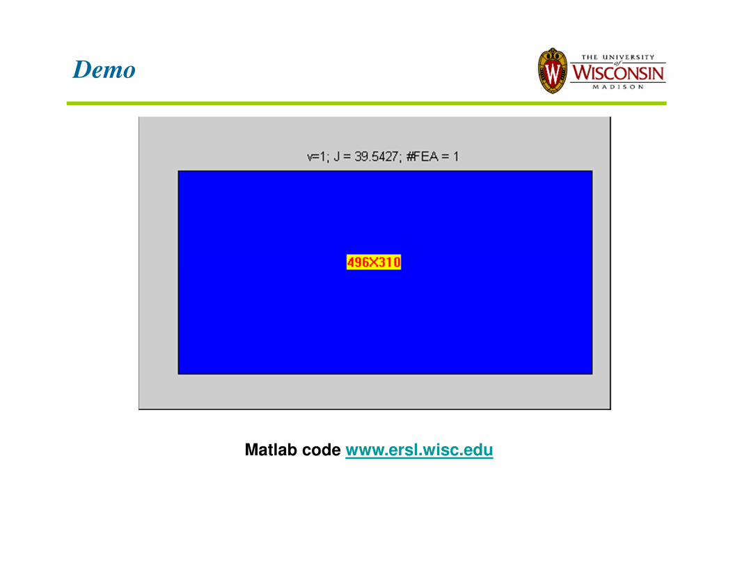
Demo
Matlab code www.ersl.wisc.edu
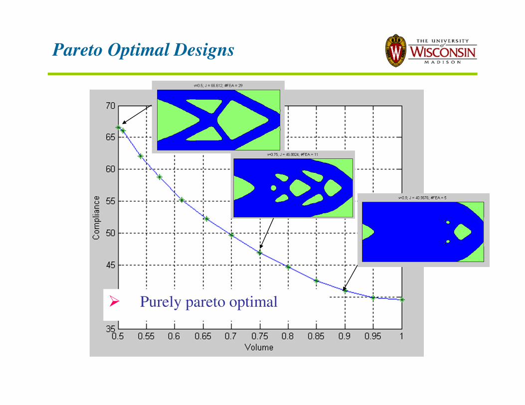
Pareto Optimal Designs
Purely pareto optimal
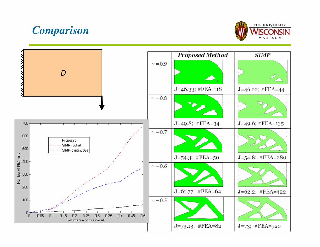
Comparison
D
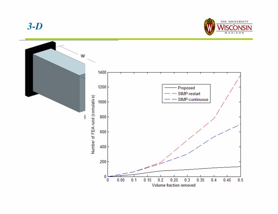
3-D
Pareto-Method SIMP
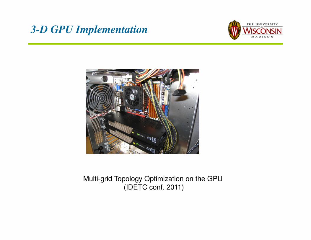
3-D GPU Implementation
Multi-grid Topology Optimization on the GPU
(IDETC conf. 2011)
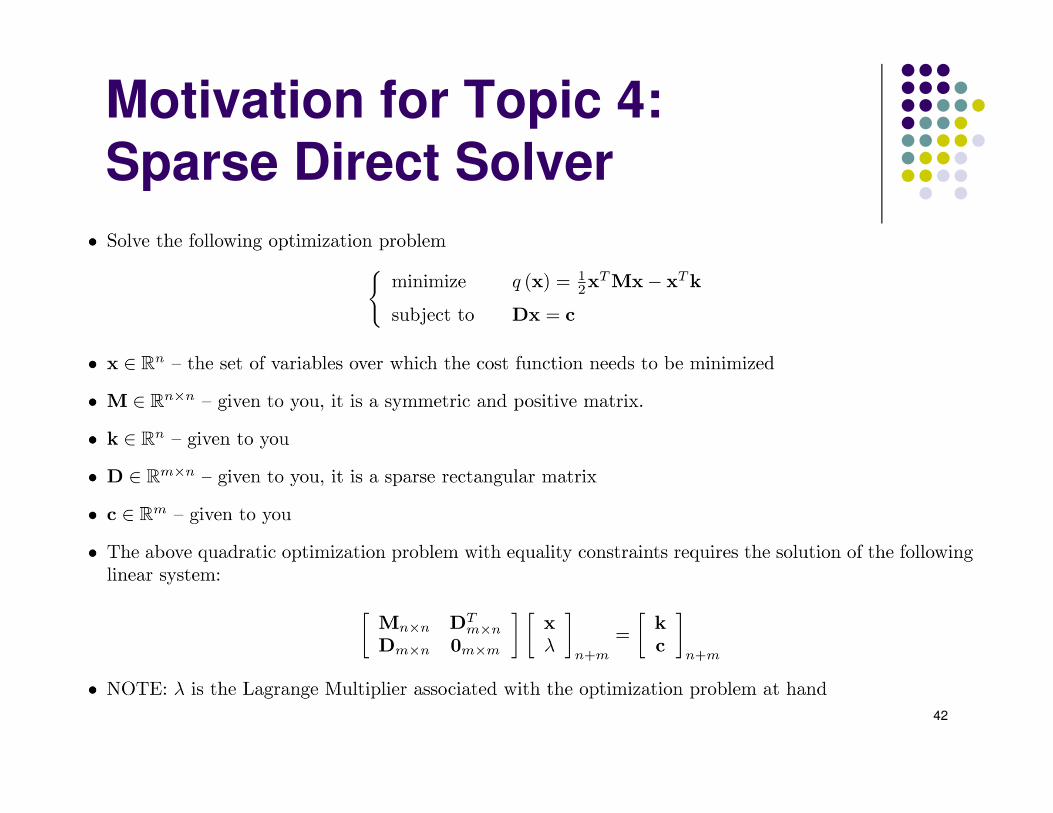
Motivation for Topic 4:Sparse Direct Solver
42
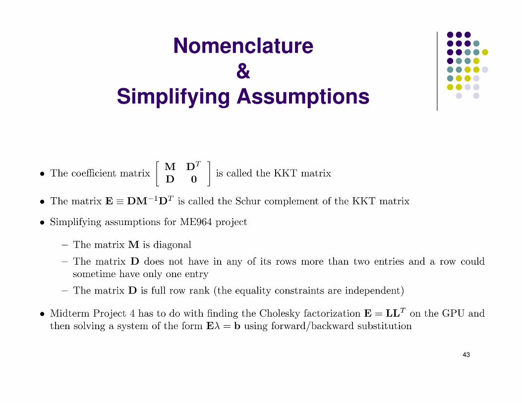
Nomenclature&
Simplifying Assumptions
43
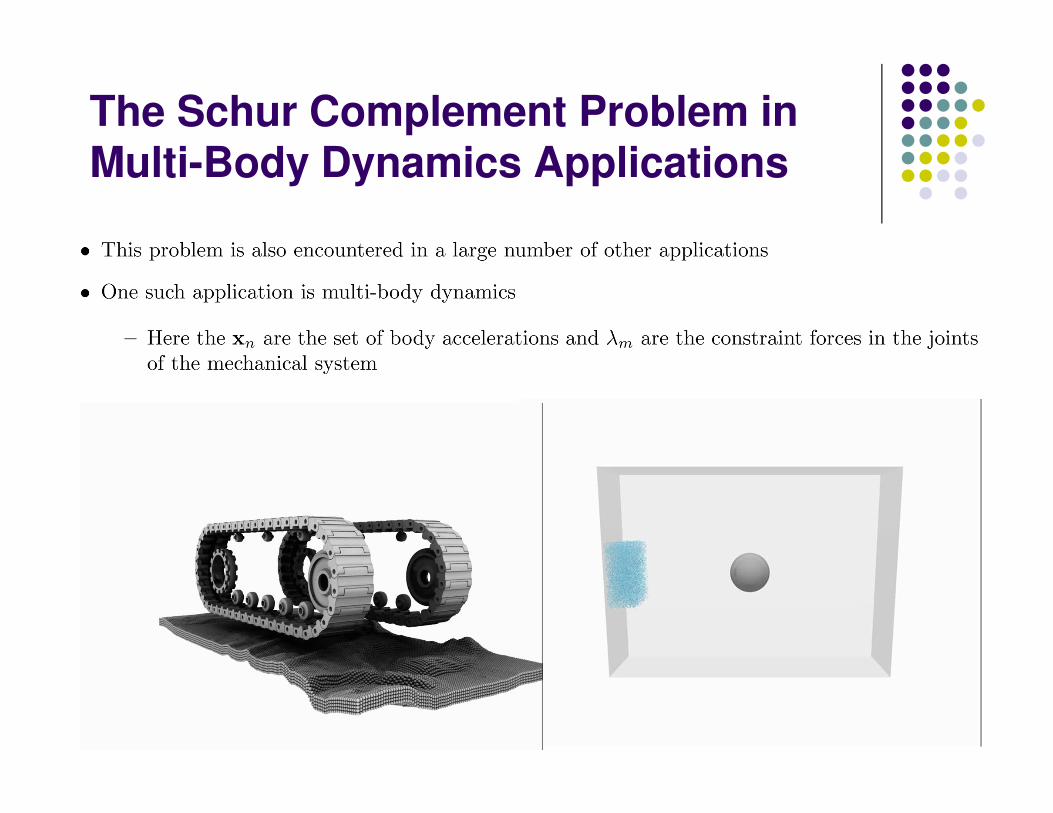
The Schur Complement Problem inMulti-Body Dynamics Applications
44
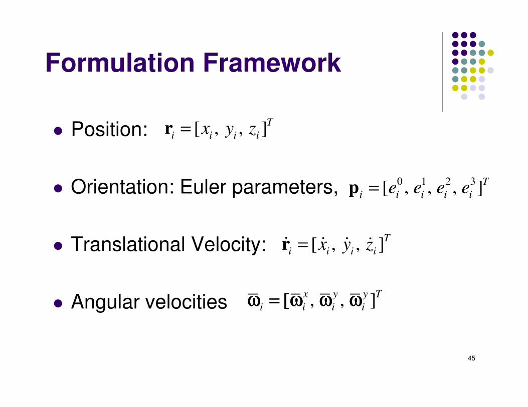
Formulation Framework
Position:
Orientation: Euler parameters,
Translational Velocity:
Angular velocities , , ]x y y T
i i i iω = [ω ω ωω = [ω ω ωω = [ω ω ωω = [ω ω ω
0 1 2 3[ , , , ]T
i i i i ie e e e=p
[ , , ]T
i i i ix y z=rɺ ɺ ɺ ɺ
[ , , ]T
i i i ix y z=r
45
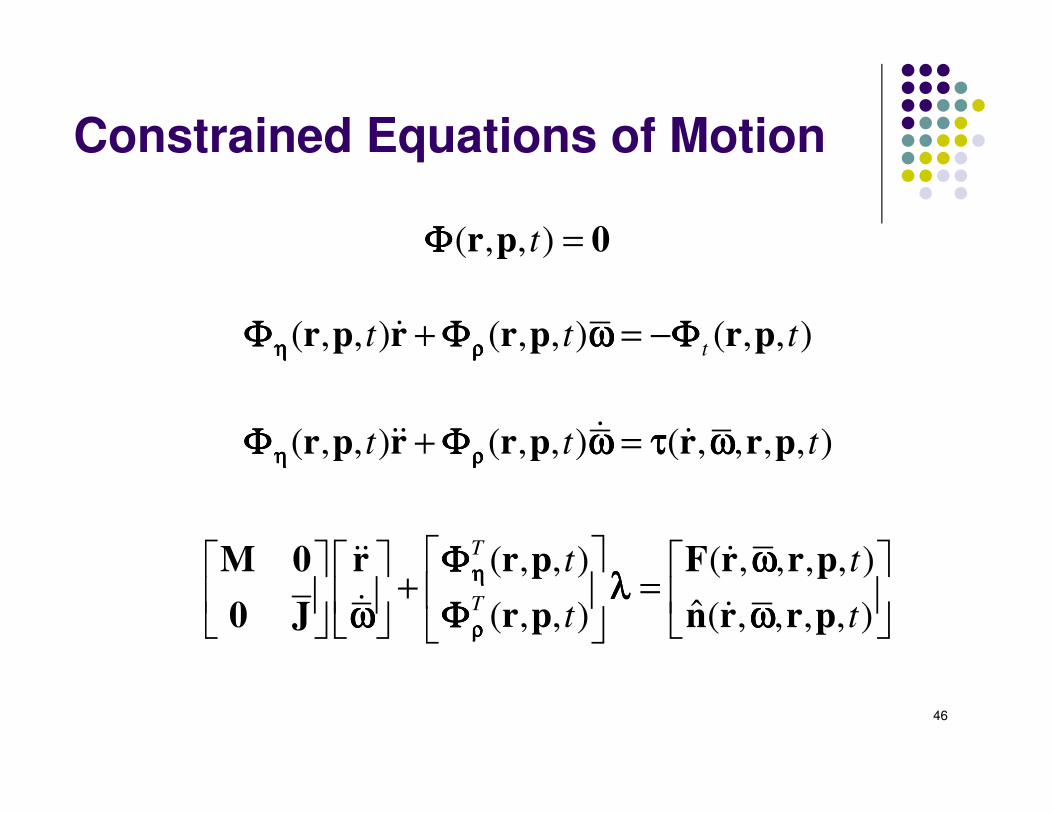
Constrained Equations of Motion
( , , )tΦΦΦΦ =r p 0
( , , ) ( , , ) ( , , )tt t tη ρη ρη ρη ρΦ Φ ω ΦΦ Φ ω ΦΦ Φ ω ΦΦ Φ ω Φ+ = −r p r r p r pɺ
( , , ) ( , , ) ( , , , , )t t tη ρη ρη ρη ρΦ Φ ω τ ωΦ Φ ω τ ωΦ Φ ω τ ωΦ Φ ω τ ω+ =r p r r p r r pɺɺɺ ɺ
( , , ) ( , , , , )
ˆ( , , ) ( , , , , )
T
T
t t
t t
ηηηη
ρρρρ
ΦΦΦΦ ωωωωλλλλ
ΦΦΦΦω ωω ωω ωω ω
+ =
r pM 0 r F r r p
r p0 J n r r p
ɺɺ ɺ
ɺ ɺ
46
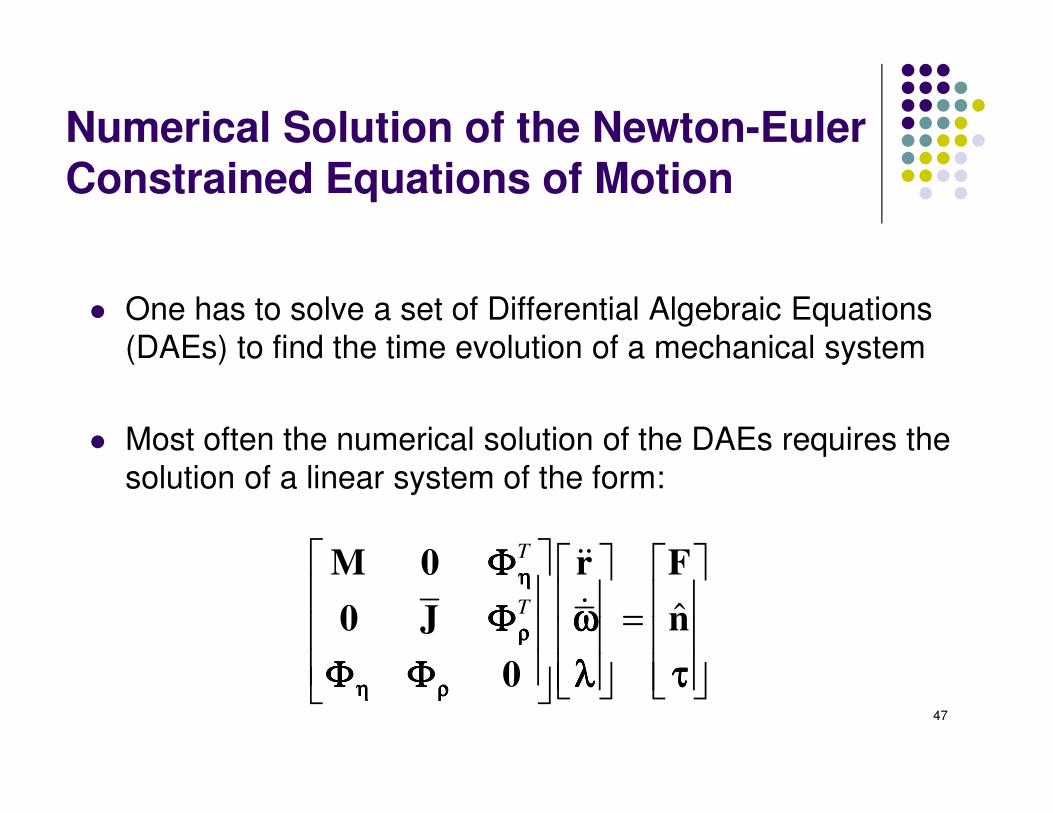
Numerical Solution of the Newton-Euler Constrained Equations of Motion
One has to solve a set of Differential Algebraic Equations
(DAEs) to find the time evolution of a mechanical system
Most often the numerical solution of the DAEs requires the
solution of a linear system of the form:
ˆ
T
T
ηηηη
ρρρρ
η ρη ρη ρη ρ
ΦΦΦΦ
Φ ωΦ ωΦ ωΦ ω
Φ Φ λ τΦ Φ λ τΦ Φ λ τΦ Φ λ τ
=
M 0 r F
0 J n
0
ɺɺ
ɺ
47
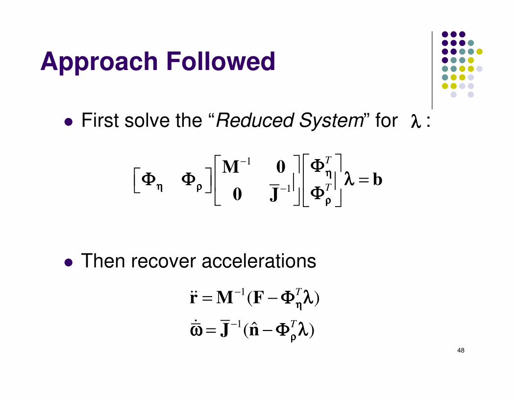
Approach Followed
First solve the “Reduced System” for :
Then recover accelerations
λλλλ
1
1
T
T
ηηηη
η ρη ρη ρη ρ
ρρρρ
ΦΦΦΦΦ Φ λΦ Φ λΦ Φ λΦ Φ λ
ΦΦΦΦ
−
−
=
M 0b
0 J
1
1
( )
ˆ( )
T
T
ηηηη
ρρρρ
Φ λΦ λΦ λΦ λ
ω Φ λω Φ λω Φ λω Φ λ
−
−
= −
= −
r M F
J n
ɺɺ
ɺ
48
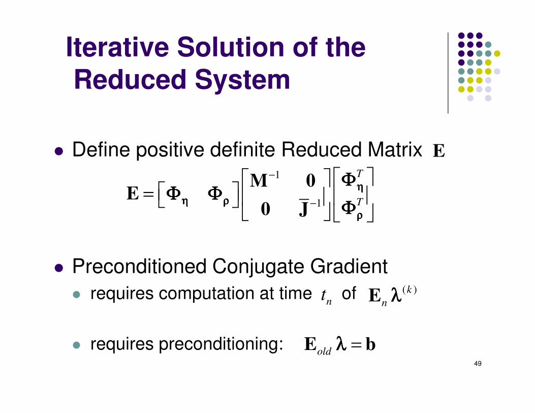
Iterative Solution of theReduced System
Define positive definite Reduced Matrix
Preconditioned Conjugate Gradient
requires computation at time of
requires preconditioning:
1
1
T
T
ηηηη
η ρη ρη ρη ρ
ρρρρ
ΦΦΦΦΦ ΦΦ ΦΦ ΦΦ Φ
ΦΦΦΦ
−
−
=
M 0E
0 J
E
nt( )k
n λλλλE
old λλλλ =E b49
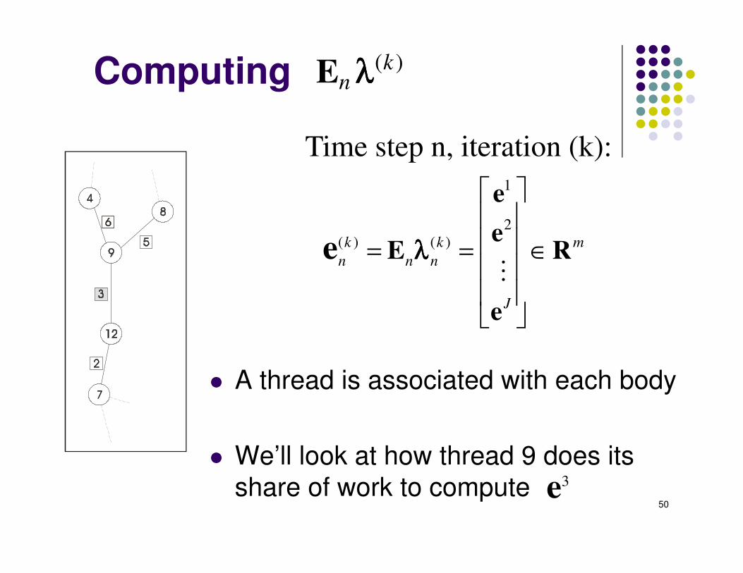
Computing
A thread is associated with each body
We’ll look at how thread 9 does its
share of work to compute
( )kn λλλλE
1
2
( ) ( )k k m
n n n
J
λλλλ
= = ∈
e
eE R
e
e⋮
3e
Time step n, iteration (k):
50
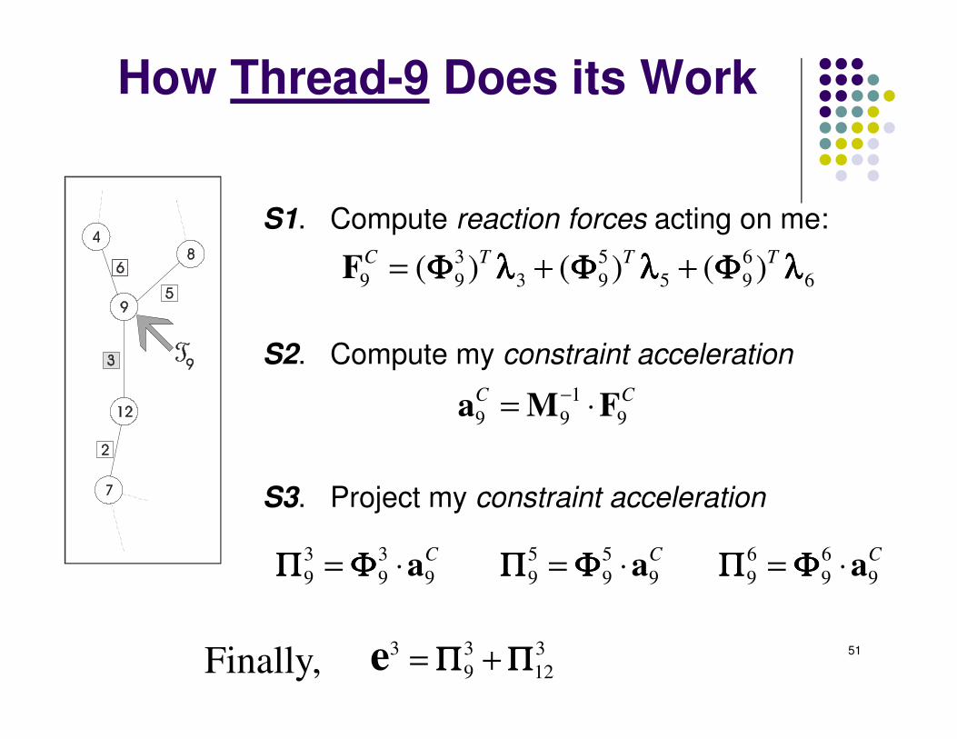
How Thread-9 Does its Work
S1. Compute reaction forces acting on me:
S2. Compute my constraint acceleration
S3. Project my constraint acceleration
3 5 6
9 9 3 9 5 9 6( ) ( ) ( )C T T TΦ λ Φ λ Φ λΦ λ Φ λ Φ λΦ λ Φ λ Φ λΦ λ Φ λ Φ λ= + +F
1
9 9 9
C C−= ⋅a M F
3 3 5 5 6 6
9 9 9 9 9 9 9 9 9
C C CΠ Φ Π Φ Π ΦΠ Φ Π Φ Π ΦΠ Φ Π Φ Π ΦΠ Φ Π Φ Π Φ= ⋅ = ⋅ = ⋅a a a
3 3 3
9 12Π ΠΠ ΠΠ ΠΠ Π= +eFinally,51
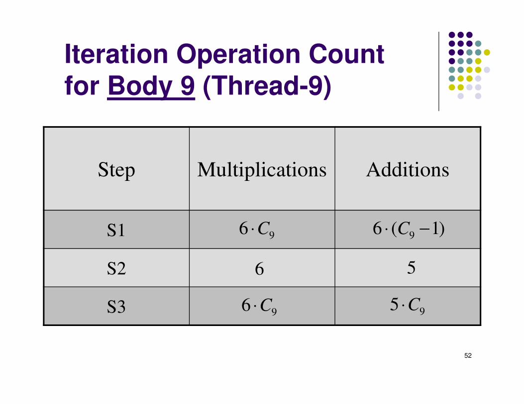
Iteration Operation Countfor Body 9 (Thread-9)
Step Multiplications Additions
S1
S2
S3
96 ( 1)C⋅ −96 C⋅
96 C⋅ 95 C⋅
56
52
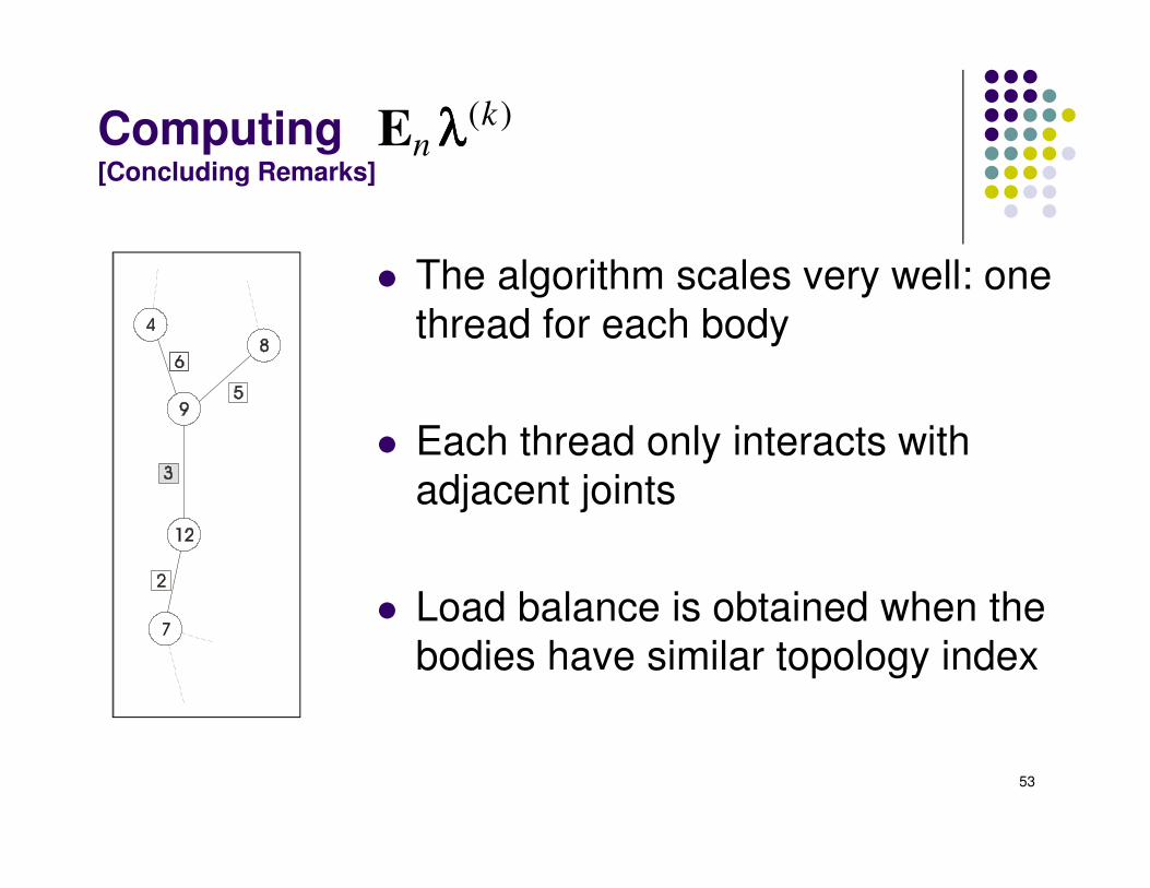
Computing [Concluding Remarks]
The algorithm scales very well: one
thread for each body
Each thread only interacts with
adjacent joints
Load balance is obtained when the
bodies have similar topology index
( )kn λλλλE
53

Direct Solution of theReduced System
54
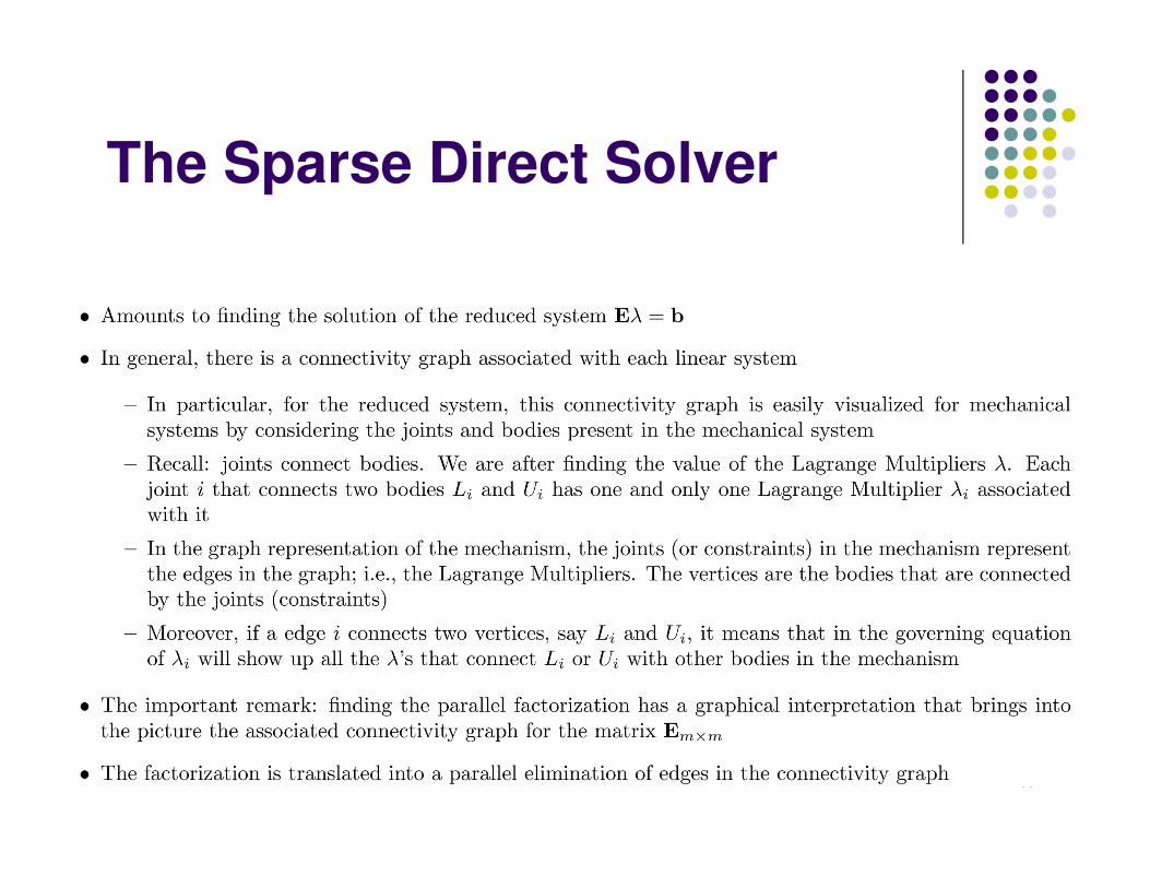
The Sparse Direct Solver
55
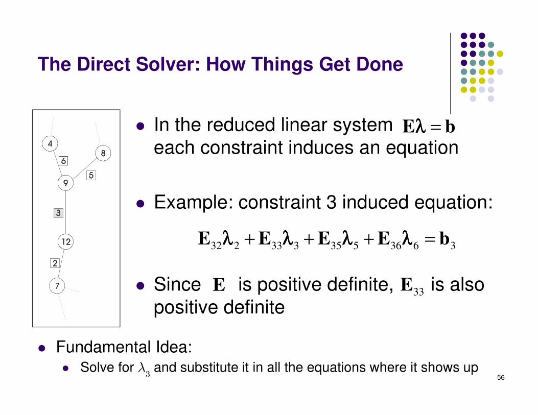
The Direct Solver: How Things Get Done
In the reduced linear system
each constraint induces an equation
Example: constraint 3 induced equation:
Since is positive definite, is also
positive definite
λλλλ =E b
32 2 33 3 35 5 36 6 3λ λ λ λλ λ λ λλ λ λ λλ λ λ λ+ + + =E E E E b
E 33E
56
Fundamental Idea: Solve for λ and substitute it in all the equations where it shows up
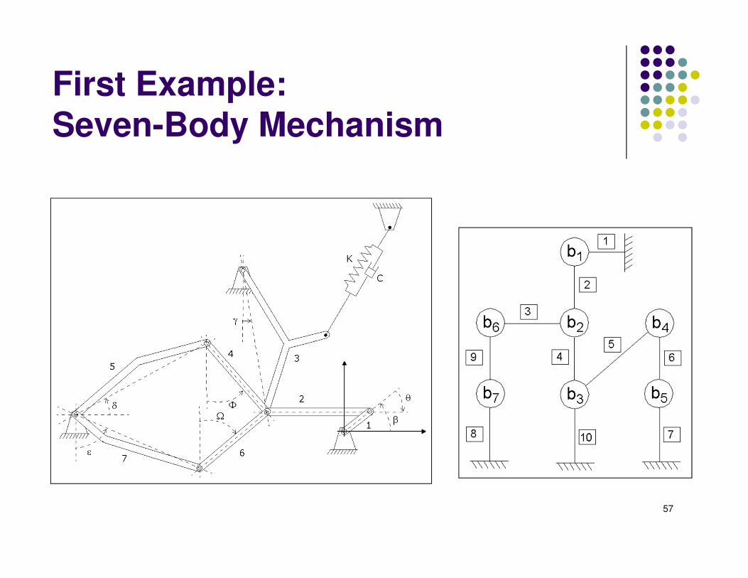
First Example: Seven-Body Mechanism
57
58
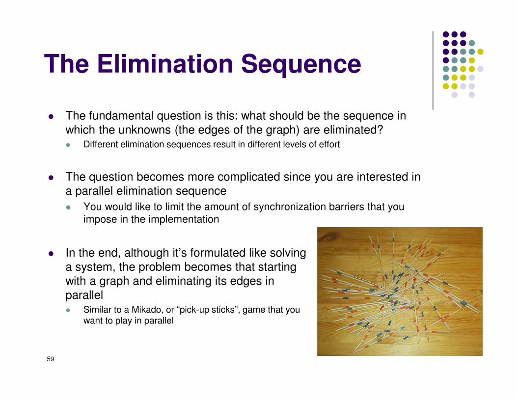
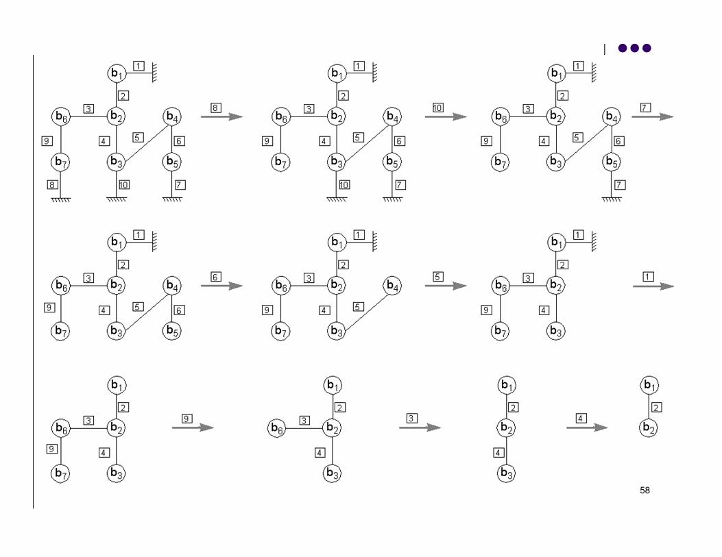
The Elimination Sequence
The fundamental question is this: what should be the sequence in
which the unknowns (the edges of the graph) are eliminated? Different elimination sequences result in different levels of effort
The question becomes more complicated since you are interested in
a parallel elimination sequence
You would like to limit the amount of synchronization barriers that you
impose in the implementation
59
In the end, although it’s formulated like solving
a system, the problem becomes that starting
with a graph and eliminating its edges in
parallel Similar to a Mikado, or “pick-up sticks”, game that you
want to play in parallel
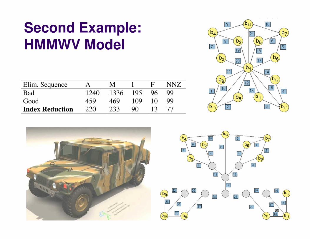
Second Example: HMMWV Model
Elim. Sequence A M I F NNZ
Bad 1240 1336 195 96 99
Good 459 469 109 10 99
Index Reduction 220 233 90 13 77
60