MCMC Methods for Multi-response Generalized

Linear Mixed Models: The MCMCglmm R Package

Jarrod HadfieldUniversity of Edinburgh

Abstract

Generalized linear mixed models provide a flexible framework for modeling a range ofdata, although with non-Gaussian response variables the likelihood cannot be obtained inclosed form. Markov chain Monte Carlo methods solve this problem by sampling from aseries of simpler conditional distributions that can be evaluated. The R package MCM-Cglmm, implements such an algorithm for a range of model fitting problems. More thanone response variable can be analysed simultaneously, and these variables are allowed tofollow Gaussian, Poisson, multi(bi)nominal, exponential, zero-inflated and censored dis-tributions. A range of variance structures are permitted for the random effects, includinginteractions with categorical or continuous variables (i.e., random regression), and morecomplicated variance structures that arise through shared ancestry, either through a pedi-gree or through a phylogeny. Missing values are permitted in the response variable(s) anddata can be known up to some level of measurement error as in meta-analysis. All sim-ulation is done in C/ C++ using the CSparse library for sparse linear systems. If youuse the software please cite this article, as published in the Journal of Statistic Software(Hadfield 2010)

Keywords: MCMC, linear mixed model, pedigree, phylogeny, animal model, multivariate,sparse, R.

Due to their flexibility, linear mixed models are now widely used across the sciences (Brownand Prescott 1999; Pinheiro and Bates 2000; Demidenko 2004). However, generalizing thesemodels to non-Gaussian data has proved difficult because integrating over the random effectsis intractable (McCulloch and Searle 2001). Although techniques that approximate these in-tegrals (Breslow and Clayton 1993) are now popular, Markov chain Monte Carlo (MCMC)methods provide an alternative strategy for marginalizing the random effects that may bemore robust (Zhao, Staudenmayer, Coull, and Wand 2006; Browne and Draper 2006). De-veloping MCMC methods for generalized linear mixed models (GLMM) is an active area ofresearch (e.g., Zeger and Karim 1991; Damien, Wakefield, and Walker 1999; Sorensen andGianola 2002; Zhao et al. 2006), and several software packages are now available that im-plement these techniques (e.g., WinBUGS (Spiegelhalter, Thomas, Best, and Lunn 2003),MLwiN (Rasbash, Steele, Browne, and Prosser 2005), glmmBUGS (Brown 2009), JAGS(Plummer 2003)). However, these methods often require a certain level of expertise on behalfof the user and may take a great deal of computing time. The MCMCglmm package for R(R Development Core Team 2009) implements Markov chain Monte Carlo routines for fittingmulti-response generalized linear mixed models. A range of distributions are supported andseveral types of variance structure for the random effects and the residuals can be fitted. Theaim is to provide routines that require little expertise on behalf of the user while reducing the

2 MCMCglmm

amount of computing time required to adequately sample the posterior distribution.

In this paper we explain the underlying structure of GLMM’s and then briefly describe ageneral strategy for estimating the parameters. Few new results are presented, and we wouldlike to acknowledge that many of the statistical results can be found in Sorensen and Gianola(2002) and many of the algorithm details that allow the models to be fitted efficiently can befound in Davis (2006). The main body of the paper introduces the software, using a workedexample taken from a quantitative genetic experiment. We end by comparing the routineswith WinBUGS (Spiegelhalter et al. 2003), and find MCMCglmm to be nearly 40 times fasterper iteration, and to have an effective sample size per iteration more than 3 times greater.

1. Model form

The model has three components: a) probability density functions that relate the data y tolatent variables l, on the link scale b) a standard linear mixed model with fixed and randompredictors applied to l and c) variance structures that describe the expected (co)variancesbetween the location effects (fixed and random effects). Although we develop these models ina Bayesian context where the distinction between fixed and random effects does not technicallyexist, we make the distinction throughout the manuscript as the terminology is well entrenchedand understood.

1.1. Probability of the data y given the latent variable l

The probability of the ith data point is represented by:

fi(yi|li) (1)

where fi is the probability density function associated with yi. For example, if yi was assumedto be Poisson distributed and we used the canonical log link function, then Equation 1 wouldhave the form:

fP (yi|λ = exp(li)) (2)

where λ is the canonical parameter of the Poisson density function fP .

1.2. Linear model for the latent variables l

The vector of latent variables are predicted by the linear model

l = Xβ + Zu + e (3)

where X is a design matrix relating fixed predictors to the data, and Z is a design matrixrelating random predictors to the data. These predictors have associated parameter vectorsβ and u, and e is a vector of residuals. In the Poisson case these residuals deal with anyover-dispersion in the data after accounting for fixed and random sources of variation.

Jarrod Hadfield 3

1.3. Variance structures for the model parameters

The location effects (β and u), and the residuals (e) are assumed to come from a multivariatenormal distribution: βu

e

∼ N β0

00

, B 0 0

0 G 00 0 R

(4)

where β0 are the prior means for the fixed effects with prior covariance matrix B, and G andR are the expected (co)variances of the random effects and residuals respectively. The zerooff-diagonal matrices imply a priori independence between fixed effects, random effects, andresiduals. Generally, G and R are large square matrices with dimensions equal to the numberof random effects and residuals. Typically they are unknown, and must be estimated from thedata, usually by assuming they are structured in a way that they can be parametrized by fewparameters. Below we will focus on the structure of G, but the same logic can be applied to R.

At its most general, MCMCglmm allows variance structures of the form:

G = (V1 ⊗A1)⊕ (V2 ⊗A2)⊕ . . . (5)

where the parameter (co)variance matrices (V) are usually low-dimensional and are to beestimated, and the structured matrices (A) are usually high dimensional and treated asknown. We will refer to terms separated by a direct sum (⊕) as component terms, and the useof a direct sum explicitly assumes random effects associated with different component termsare independent. Each component term, however, is formed through the Kronecker product(⊗) which allows for possible dependence between random effects within a component term.Equation 24 can be expanded to give:

G =

[V1 ⊗A1 0

0 V2 ⊗A2

](6)

where the zero off-diagonals represent the independence between component terms.

In the simplest models the structured matrices of each component term are often assumed tobe identity matrices and the parameter (co)variance matrices scalar variances:

V1 ⊗A1 = σ21I (7)

which assumes that random effects within a component term are independent but have acommon variance. However, independence between different levels is often too strong anassumption. For example, if we had made two visits to a sample of schools and recorded testscores for the children, we may expect dependence between measurements made in the sameschool although they were sampled at different times. If the random effects are ordered schoolswithin ages (u> = [u1 u2]) where u1 are the random effects for the schools at time periodone, and u2 for the same set of schools at time period 2, then an appropriate G componentmay have the form:

4 MCMCglmm

V1 ⊗A1 =

[σ2u1 σu1,u2σu2,u1 σ2u2

]⊗ I (8)

Here the diagonal elements model different variances for the two sampling periods, and thecovariance captures any persistent differences between schools. The identity matrix in theKronecker product implies the schools are independent. Although the assumption of inde-pendence may be adequate in many applications, there are situations where it is not tenable.For example, when data have been collected on related individuals, or related species, thencomplicated patterns of dependence can arise if the characteristics are heritable. In thesecases A is not an identity matrix but a matrix whose elements are equal to the proportion ofgenes the two individuals have in common.

2. Parameter estimation and DIC

For most types of model (non-Gaussian data) the distribution of l is not in a recognizableform and is updated using either Metropolis-Hastings updates or the slice sampling methodof (Damien et al. 1999). Latent variables whose residuals are non-independent are sampled inblocks using Metropolis-Hastings updates and an efficient proposal distribution is determinedduring the burn-in phase using adaptive methods (Haario, Saksman, and Tamminen 2001;Ovaskainen, Rekola, Meyke, and Arjas 2008). The parameters of the mixed model (β and u)follow a multivariate normal distribution and can be Gibbs sampled in a single block usingthe method of Garcia-Cortes and Sorensen (2001). This method requires solving a large, butoften sparse set of linear equations which can be done efficiently using methods provided inthe CSparse library (Davis 2006). With conjugate priors the variance structures (R and G)follow an inverse-Wishart distribution which can also be Gibbs sampled in a single block inmany instances. By fitting non-identified multiplicative working parameters for the randomeffects non-central F -distributed priors for the variance components can be fitted (Gelman2006). This involves updating the working parameters each iteration which again can beachieved using the method of Garcia-Cortes and Sorensen (2001).

The deviance and hence the deviance information criterion (DIC) can be calculated in dif-ferent ways depending on what is in ‘focus’ (Spiegelhalter, Best, Carlin, and van der Linde2002). For non-Gaussian response variables (including censored Gaussian) MCMCglmm cal-culates the deviance using the probability of the data given the latent variables. For Gaussiandata, however, the deviance is calculated using the probability of the data given the locationparameters θ> = [β u].

In the appendix the conditional distributions, and computational strategies for sampling fromthem, are described in more detail, together with a more in depth explanation on the com-putation of deviance and DIC.

3. Software

To illustrate the software we reanalyze experimental data collected on the Eurasian passerinebird, the Blue tit (Cyanistes caeruleus) (Hadfield, Nutall, Osorio, and Owens 2007). The

Jarrod Hadfield 5

data consist of measurements taken on 828 chicks distributed across 106 broods:

R> library("MCMCglmm")

R> data("BTdata")

R> BTdata[1,]

tarsus back animal dam fosternest hatchdate sex

1 -1.892297 1.146421 R187142 R187557 F2102 -0.6874021 Fem

The day after the chicks hatch, approximately half of the brood are reciprocally swapped withchicks from another nest. This results in an unbalanced cross-classified data structure wherechicks share a fosternest with both relatives and non-relatives. Using molecular methods(Griffiths, Double, Orr, and Dawson 1998) the sex of the chicks were determined in 94% ofcases, and the response variables, tarsus length and back color, were measured in all birds.The response variables are approximately normal and were mean centered and scaled to unitvariance. The date on which the chicks hatched was recorded for all nests. The parentalgeneration is assumed to consist of unrelated individuals and all chicks from the same familyare assumed to share the same mother and father. Although in this example, family structurecan be modeled more efficiently by fitting genetic mother (dam) as a random effect, we willuse the more general animal model Henderson (1976) which is parametrized in terms of therelationship matrix, A. The relationship matrix is defined by the pedigree;

R> data("BTped")

R> BTped[1,]

animal dam sire

1 R187557 <NAR> <NAR>

a 3 column data frame with an individual’s identifier (animal) in the first column and itsparental identifiers in the second and third columns. The pedigree often contains more in-dividuals than are present in the data frame (in this example the pedigree also includes theparental generation) but all animal’s in the data frame must have a row in the pedigree.

3.1. MCMCglmm arguments

The function MCMCglmm within the R library of the same name is used for model fitting.Hadfield et al. (2007) were interested in estimating the covariance between tarsus and back

for different sources of variation and to achieve this we fitted the model:

R> m1<-MCMCglmm(cbind(tarsus, back) ~ trait:sex + trait:hatchdate - 1,

R> random = ~ us(trait):animal + us(trait):fosternest, rcov = ~ us(trait):units,

R> prior = prior, family = rep("gaussian", 2), nitt = 60000, burnin = 10000,

R> thin=25, data = BTdata, pedigree=BTped)

In the following sections we work through the four main arguments taken by MCMCglmm: thosethat specify the response variables and fixed effects (fixed), the distribution of the responsevariables (family), the random effects and associated G-structure (random), and the R-structure (rcov). The syntax used to specify the model closely follows that used by asreml(Butler, Cullis, Gilmour, and Gogel 2007), an R interface to ASReml (Gilmour, Gogel, Cullis,

6 MCMCglmm

Welham, and Thompson 2002) - a program for fitting GLMM using restricted maximum like-lihood (REML).

3.2. fixed: Response variables and fixed effects

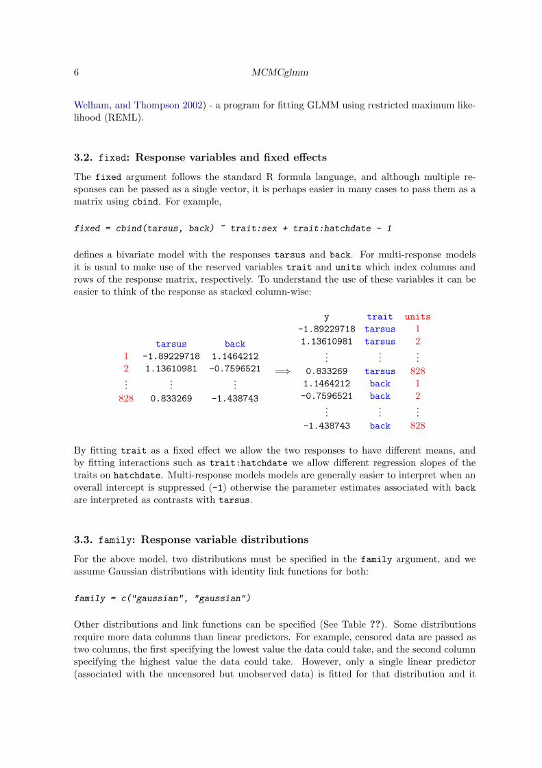
The fixed argument follows the standard R formula language, and although multiple re-sponses can be passed as a single vector, it is perhaps easier in many cases to pass them as amatrix using cbind. For example,

fixed = cbind(tarsus, back) ~ trait:sex + trait:hatchdate - 1

defines a bivariate model with the responses tarsus and back. For multi-response modelsit is usual to make use of the reserved variables trait and units which index columns androws of the response matrix, respectively. To understand the use of these variables it can beeasier to think of the response as stacked column-wise:

tarsus back

1 -1.89229718 1.1464212

2 1.13610981 -0.7596521...

......

828 0.833269 -1.438743

=⇒

y trait units

-1.89229718 tarsus 11.13610981 tarsus 2

......

...0.833269 tarsus 8281.1464212 back 1-0.7596521 back 2

......

...-1.438743 back 828

By fitting trait as a fixed effect we allow the two responses to have different means, andby fitting interactions such as trait:hatchdate we allow different regression slopes of thetraits on hatchdate. Multi-response models models are generally easier to interpret when anoverall intercept is suppressed (-1) otherwise the parameter estimates associated with back

are interpreted as contrasts with tarsus.

3.3. family: Response variable distributions

For the above model, two distributions must be specified in the family argument, and weassume Gaussian distributions with identity link functions for both:

family = c("gaussian", "gaussian")

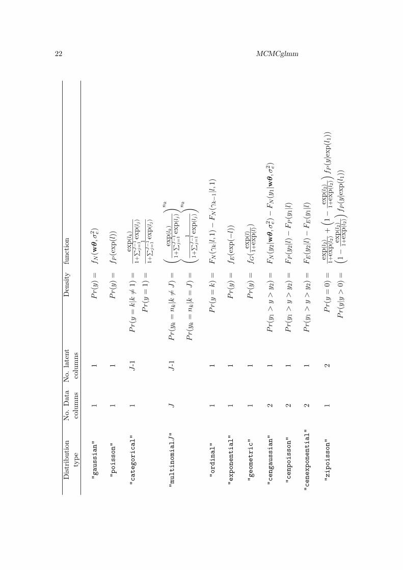
Other distributions and link functions can be specified (See Table ??). Some distributionsrequire more data columns than linear predictors. For example, censored data are passed astwo columns, the first specifying the lowest value the data could take, and the second columnspecifying the highest value the data could take. However, only a single linear predictor(associated with the uncensored but unobserved data) is fitted for that distribution and it

Jarrod Hadfield 7

should be remembered that in this case trait is really indexing linear predictors, not data.Another example of this is the binomial distribution (specified as "multinomial2" in thefamily argument) which is generally specified as a two column response of successes andfailures, but is parametrized by a single linear predictor of the log odds ratio. In addition,some distributions actually have more linear predictors than data columns. For example, thezero-inflated Poisson has two linear predictors; one for predicting zero-inflation and one forpredicting the Poisson counts. Similarly, categorical data although passed as a single responseare treated as a multinomial response with J − 1 linear predictors (where J are the numberof categories). Again, it should be remembered that in this case several levels of trait maybe associated with different aspects of the same data column.

3.4. random: Random effects and G

Simple variance structures, as represented in Equation 7, can also be specified as a standardR formula:

random = ~ fosternest + ...

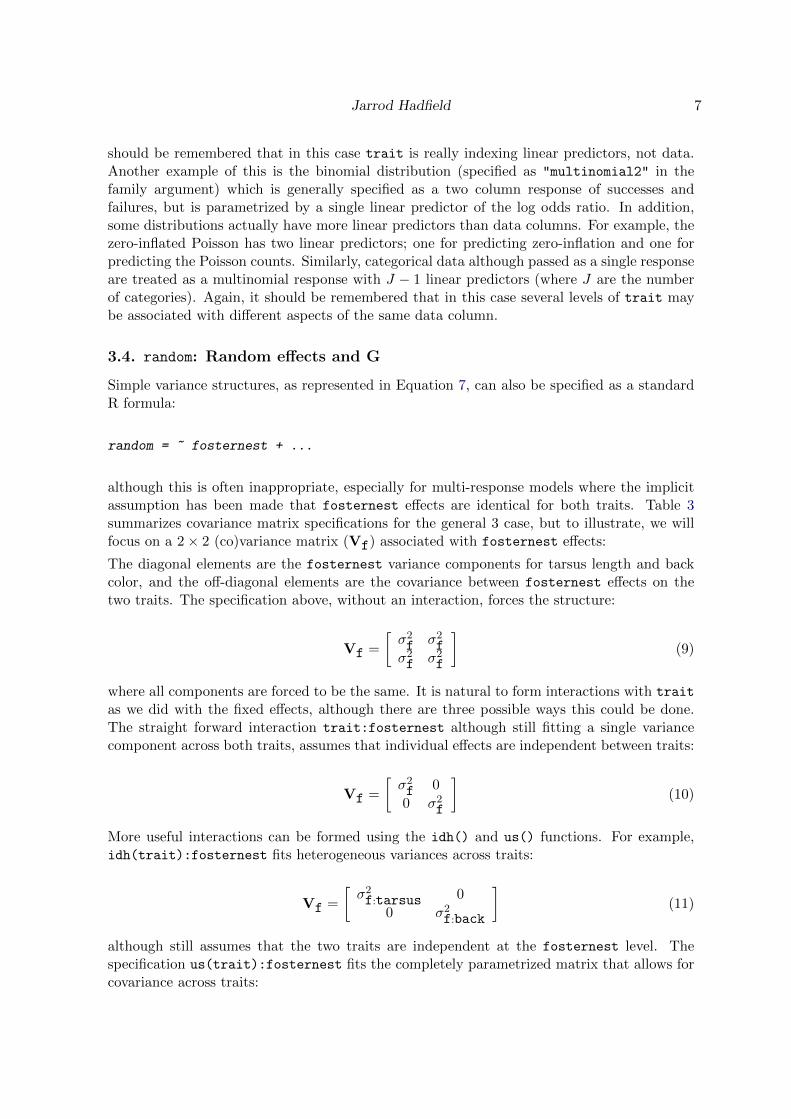
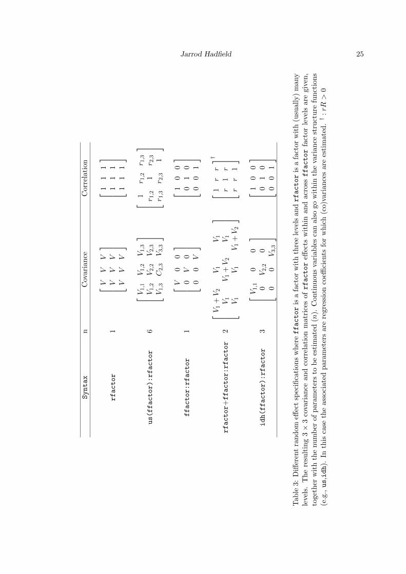
although this is often inappropriate, especially for multi-response models where the implicitassumption has been made that fosternest effects are identical for both traits. Table 3summarizes covariance matrix specifications for the general 3 case, but to illustrate, we willfocus on a 2× 2 (co)variance matrix (Vf) associated with fosternest effects:

The diagonal elements are the fosternest variance components for tarsus length and backcolor, and the off-diagonal elements are the covariance between fosternest effects on thetwo traits. The specification above, without an interaction, forces the structure:

Vf =

[σ2f σ2fσ2f σ2f

](9)

where all components are forced to be the same. It is natural to form interactions with trait

as we did with the fixed effects, although there are three possible ways this could be done.The straight forward interaction trait:fosternest although still fitting a single variancecomponent across both traits, assumes that individual effects are independent between traits:

Vf =

[σ2f 0

0 σ2f

](10)

More useful interactions can be formed using the idh() and us() functions. For example,idh(trait):fosternest fits heterogeneous variances across traits:

Vf =

[σ2f:tarsus 0

0 σ2f:back

](11)

although still assumes that the two traits are independent at the fosternest level. Thespecification us(trait):fosternest fits the completely parametrized matrix that allows forcovariance across traits:

8 MCMCglmm

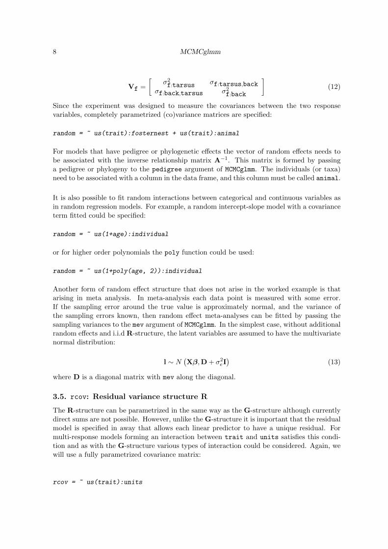
Vf =

[σ2f:tarsus σf:tarsus,back

σf:back,tarsus σ2f:back

](12)

Since the experiment was designed to measure the covariances between the two responsevariables, completely parametrized (co)variance matrices are specified:

random = ~ us(trait):fosternest + us(trait):animal

For models that have pedigree or phylogenetic effects the vector of random effects needs tobe associated with the inverse relationship matrix A−1. This matrix is formed by passinga pedigree or phylogeny to the pedigree argument of MCMCglmm. The individuals (or taxa)need to be associated with a column in the data frame, and this column must be called animal.

It is also possible to fit random interactions between categorical and continuous variables asin random regression models. For example, a random intercept-slope model with a covarianceterm fitted could be specified:

random = ~ us(1+age):individual

or for higher order polynomials the poly function could be used:

random = ~ us(1+poly(age, 2)):individual

Another form of random effect structure that does not arise in the worked example is thatarising in meta analysis. In meta-analysis each data point is measured with some error.If the sampling error around the true value is approximately normal, and the variance ofthe sampling errors known, then random effect meta-analyses can be fitted by passing thesampling variances to the mev argument of MCMCglmm. In the simplest case, without additionalrandom effects and i.i.d R-structure, the latent variables are assumed to have the multivariatenormal distribution:

l ∼ N(Xβ,D + σ2eI

)(13)

where D is a diagonal matrix with mev along the diagonal.

3.5. rcov: Residual variance structure R

The R-structure can be parametrized in the same way as the G-structure although currentlydirect sums are not possible. However, unlike the G-structure it is important that the residualmodel is specified in away that allows each linear predictor to have a unique residual. Formulti-response models forming an interaction between trait and units satisfies this condi-tion and as with the G-structure various types of interaction could be considered. Again, wewill use a fully parametrized covariance matrix:

rcov = ~ us(trait):units

Jarrod Hadfield 9

3.6. prior: Response variables and fixed effects

If not defined, default priors are used which are not proper and this can lead to both inferen-tial and numerical problems. The prior specification is passed to MCMCglmm via the argumentprior which takes a list of three elements specifying the priors for the fixed effects (B), theG-structure (G) and the R-structure (R).

For the fixed effects, a multivariate normal prior distribution can be specified through themean vector mu (β0) and a (co)variance matrix V (B) passed as list elements of B. The defaulthas a zero mean vector and a diagonal variance matrix with large variances (1e+10).

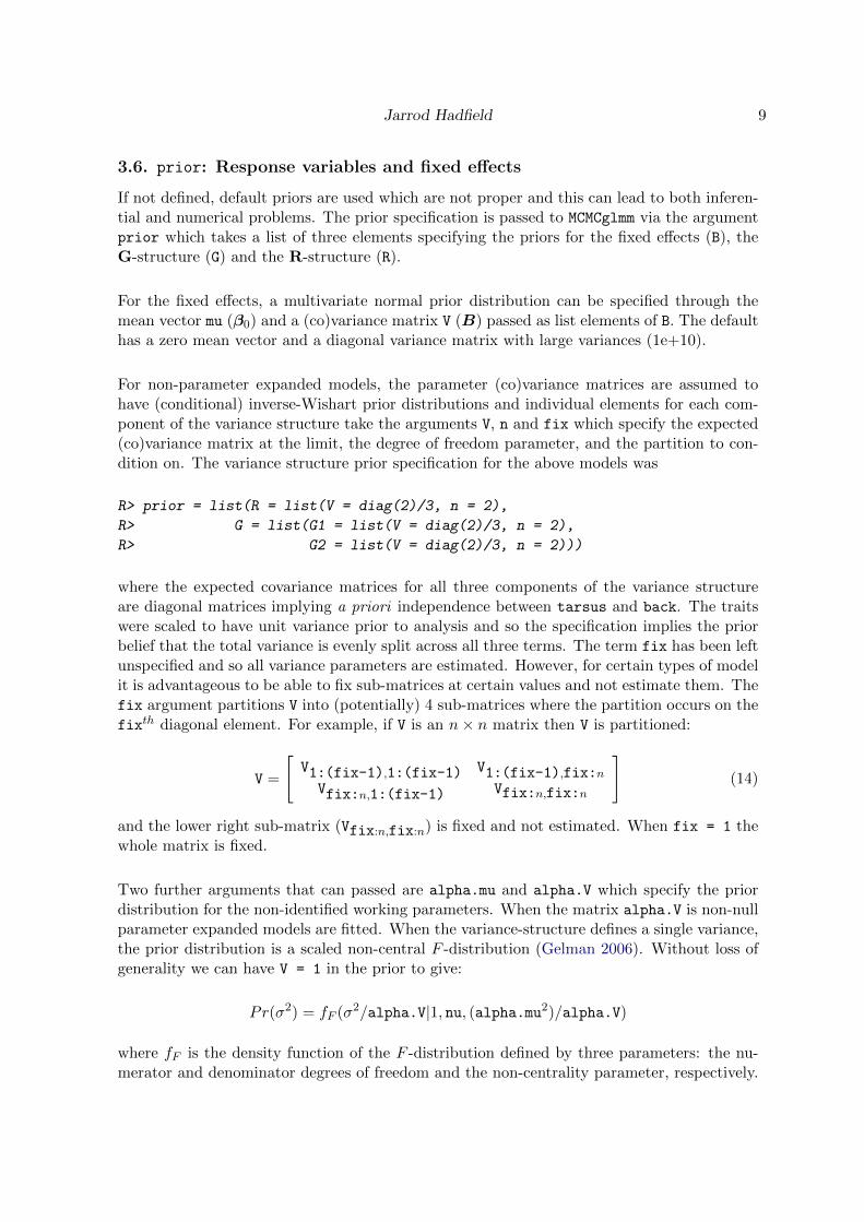
For non-parameter expanded models, the parameter (co)variance matrices are assumed tohave (conditional) inverse-Wishart prior distributions and individual elements for each com-ponent of the variance structure take the arguments V, n and fix which specify the expected(co)variance matrix at the limit, the degree of freedom parameter, and the partition to con-dition on. The variance structure prior specification for the above models was

R> prior = list(R = list(V = diag(2)/3, n = 2),

R> G = list(G1 = list(V = diag(2)/3, n = 2),

R> G2 = list(V = diag(2)/3, n = 2)))

where the expected covariance matrices for all three components of the variance structureare diagonal matrices implying a priori independence between tarsus and back. The traitswere scaled to have unit variance prior to analysis and so the specification implies the priorbelief that the total variance is evenly split across all three terms. The term fix has been leftunspecified and so all variance parameters are estimated. However, for certain types of modelit is advantageous to be able to fix sub-matrices at certain values and not estimate them. Thefix argument partitions V into (potentially) 4 sub-matrices where the partition occurs on thefixth diagonal element. For example, if V is an n× n matrix then V is partitioned:

V =

[V1:(fix-1),1:(fix-1) V1:(fix-1),fix:n

Vfix:n,1:(fix-1) Vfix:n,fix:n

](14)

and the lower right sub-matrix (Vfix:n,fix:n) is fixed and not estimated. When fix = 1 thewhole matrix is fixed.

Two further arguments that can passed are alpha.mu and alpha.V which specify the priordistribution for the non-identified working parameters. When the matrix alpha.V is non-nullparameter expanded models are fitted. When the variance-structure defines a single variance,the prior distribution is a scaled non-central F -distribution (Gelman 2006). Without loss ofgenerality we can have V = 1 in the prior to give:

Pr(σ2) = fF (σ2/alpha.V|1, nu, (alpha.mu2)/alpha.V)

where fF is the density function of the F -distribution defined by three parameters: the nu-merator and denominator degrees of freedom and the non-centrality parameter, respectively.

10 MCMCglmm

animal fosternest units DICvariance function variance function variance function

us us us 4043.8/4041.9idh us us 4050.5/4050.7idh idh us 4063.0/4062.8idh idh idh 4077.9/4076.7us idh us 4056.2/4059.2us idh idh 4091.1/4089.5idh us idh 4069.8/4069.9us us idh 4081.8/4082.4

Table 1: Deviance Information Criteria for several models where the covariance between theresponse variable for a designated source of variation was either estimated (us) or set to zero(idh). Each model was ran twice in order to asses the level of Monte Carlo error in calculatingDIC.

3.7. MCMC output

The model was ran for 60,000 iterations with a burn-in phase of 10,000 and a thinning intervalof 25. MCMCglmm returns a list with elements:

• Sol: Posterior distribution of location effects (and cutpoints for ordinal models)

• VCV: Posterior distribution of (co)variance matrices

• Liab: Posterior Distribution of latent variables

• Deviance: Deviance

• DIC: Deviance Information Criterion

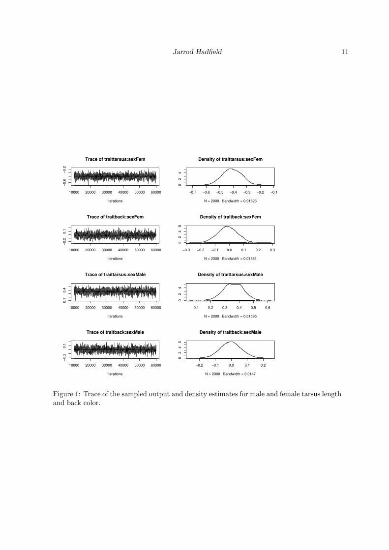
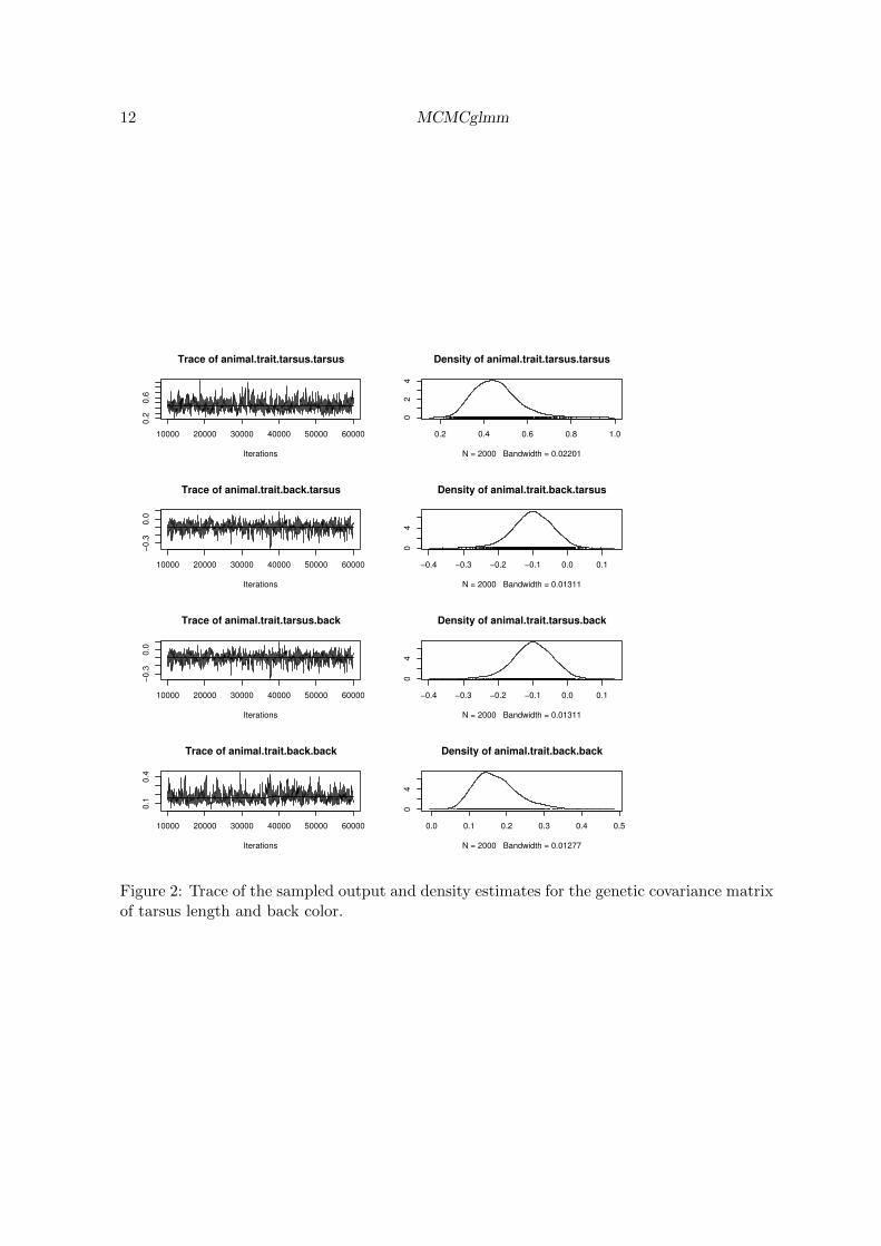
The samples from the posterior distribution are stored as mcmc objects, which can be sum-marized and visualized using the coda package (Plummer, Best, Cowles, and Vines 2008).The element Sol contains the fixed effects (β), and if pr=TRUE then also the random effects(u). The element VCV contains the parameter (co)variance matrices stacked column-wise,and if pl=TRUE then Liab contains the posterior distribution of latent variables l. The ele-ment Deviance contains the deviance at each stored iteration and DIC contains the devianceinformation criterion (Spiegelhalter et al. 2002) calculated over all iterations after burn-in.Traces of the sampled output and density estimates are shown for the effects of gender on traitexpression (Figure 1) and the genetic covariance matrix associated with animal (See Figure 2).

We also fitted alternative variance structures where some or all covariances were set to zero,and Table 1 shows the DIC for each model. The priors on the reduced models were set up sothat the marginal prior for the variances was the same as that in the full model. The samplingerror of DIC can be large and so we ran all models for an additional 500,000 iterations.

Jarrod Hadfield 11

10000 20000 30000 40000 50000 60000

−0.6

−0.2

Iterations

Trace of traittarsus:sexFem

−0.7 −0.6 −0.5 −0.4 −0.3 −0.2 −0.1

02

4

N = 2000 Bandwidth = 0.01623

Density of traittarsus:sexFem

10000 20000 30000 40000 50000 60000

−0.2

0.1

Iterations

Trace of traitback:sexFem

−0.3 −0.2 −0.1 0.0 0.1 0.2 0.3

02

46

N = 2000 Bandwidth = 0.01581

Density of traitback:sexFem

10000 20000 30000 40000 50000 60000

0.1

0.4

Iterations

Trace of traittarsus:sexMale

0.1 0.2 0.3 0.4 0.5 0.6

02

4

N = 2000 Bandwidth = 0.01595

Density of traittarsus:sexMale

10000 20000 30000 40000 50000 60000

−0.2

0.1

Iterations

Trace of traitback:sexMale

−0.2 −0.1 0.0 0.1 0.2

02

46

N = 2000 Bandwidth = 0.0147

Density of traitback:sexMale

Figure 1: Trace of the sampled output and density estimates for male and female tarsus lengthand back color.

12 MCMCglmm

10000 20000 30000 40000 50000 60000

0.2

0.6

Iterations

Trace of animal.trait.tarsus.tarsus

0.2 0.4 0.6 0.8 1.0

02

4

N = 2000 Bandwidth = 0.02201

Density of animal.trait.tarsus.tarsus

10000 20000 30000 40000 50000 60000

−0.3

0.0

Iterations

Trace of animal.trait.back.tarsus

−0.4 −0.3 −0.2 −0.1 0.0 0.1

04

N = 2000 Bandwidth = 0.01311

Density of animal.trait.back.tarsus

10000 20000 30000 40000 50000 60000

−0.3

0.0

Iterations

Trace of animal.trait.tarsus.back

−0.4 −0.3 −0.2 −0.1 0.0 0.1

04

N = 2000 Bandwidth = 0.01311

Density of animal.trait.tarsus.back

10000 20000 30000 40000 50000 60000

0.1

0.4

Iterations

Trace of animal.trait.back.back

0.0 0.1 0.2 0.3 0.4 0.5

04

N = 2000 Bandwidth = 0.01277

Density of animal.trait.back.back

Figure 2: Trace of the sampled output and density estimates for the genetic covariance matrixof tarsus length and back color.

Jarrod Hadfield 13

3.8. Comparison with WinBUGS

We also fitted an identical model in WinBUGS (code available from the author) using amultivariate extension to the method proposed by Waldmann (2009). On a 2.5Ghz dualcore MacBook Pro with 2GB RAM, MCMCglmm took 7.6 minutes and WinBUGS took4.8 hours to fit the model. Moreover, the number of effective samples was 3.2 times higherin MCMCglmm (averaged over all parameters) indicating that the chain has better mixingproperties. Because MCMCglmm samples all location parameters in a single block the gainsin efficiency are expected to be even higher when the parameters show stronger posteriorcorrelation.

14 MCMCglmm

4. Concluding remarks

This paper introduces an R package for fitting multi-response generalized linear mixed mod-els using Markov chain Monte Carlo techniques developed in quantitative genetics (Sorensenand Gianola 2002). A key aspect of these techniques is that they update all location effects(fixed and random) as a single block which results in better mixing properties and shorterchain lengths than alternative strategies. This can involve repeatedly solving a very large butsparse set of mixed model equations, and the computational cost of doing this is minimized byusing the CSparse C libraries for solving sparse linear systems (Davis 2006). For the exampledata set analysed, MCMCglmm collected 120 times more effective samples per unit time thanthe same model fitted in WinBUGS. A range of distributions for the response variables arepermitted, and flexible variance structures for the random effects and residuals included. Itis hoped that this package makes the flexibility and simplicity of generalized linear mixedmodeling available to a wider range of researchers.

Acknowledgements

This work would not have been possible without the CSparse written by Tim Davis and thecomprehensive book on MCMC and mixed models by Sorensen & Gianola. This work wasfunded by NERC and a Leverhulme trust award to Loeske Kruuk, who together with ShinichiNakagawa and two anonymous reviewers made helpful comments on this manuscript. I alsothank Dylan Childs for help with fitting the example in WinBUGS.

References

Breslow NE, Clayton DG (1993). “Approximate inference in generalized linear mixed models.”Journal of the American Statistical Association, 88(421), 9–25.

Brown H, Prescott R (1999). Applied Mixed Models in Medicine. Statistics in Practice. JohnWiley & Sons, New York.

Brown P (2009). glmmBUGS: Generalized Linear Mixed Models and Spatial Models withBUGS. R package version 1.6.4, URL http://CRAN.R-project.org/package=glmmBUGS.

Browne W, Draper D (2006). “A comparison of Bayesian and likelihood-based methods forfitting multilevel models.” Bayesian Analysis, 1(3), 473–514.

Browne WJ, Steele F, Golalizadeh M, Green MJ (2009). “The use of simple reparameter-izations to improve the efficiency of Markov chain Monte Carlo estimation for multilevelmodels with applications to discrete time survival models.” Journal of the Royal StatisticalSociety Series A - Statistics in Society, 172, 579–598.

Butler D, Cullis BR, Gilmour AR, Gogel BJ (2007). Analysis of Mixed Models for S–languageEnvironments: ASReml–R Reference Manual. Queensland DPI, Brisbane, Australia. URLhttp://www.vsni.co.uk/resources/doc/asreml-R.pdf.

Jarrod Hadfield 15

Cowles MK (1996). “Accelerating Monte Carlo Markov chain convergence for cumulative–linkgeneralized linear models.” Statistics and Computing, 6(2), 101–111.

Damien P, Wakefield J, Walker S (1999). “Gibbs sampling for Bayesian non–conjugate andhierarchical models by using auxiliary variables.” Journal of the Royal Statistical SocietySeries B-Statistical Methodology, 61, 331–344.

Davis TA (2006). Direct Methods for Sparse Linear Systems. Fundamentals of Algorithms.SIAM, Philadelphia.

Demidenko E (2004). Mixed Models: Theory and Application. Wiley Series in Probabilityand Statistics. John Wiley & Sons, New Jersey.

Garcia-Cortes LA, Sorensen D (2001). “Alternative implementations of Monte Carlo EMalgorithms for likelihood inferences.” Genetics Selection Evolution, 33(4), 443–452.

Gelman A (2006). “Prior distributions for variance parameters in hierarchical models.”Bayesian Analysis, 1(3), 515–533.

Gelman A, Carlin JB, Stern HS, Rubin DB (2004). Bayesian Data Analysis. Texts in Statis-tical Science. Chapman & Hall, 2nd edition.

Gelman A, van Dyk DA, Huang ZY, Boscardin WJ (2008). “Using redundant parameteriza-tions to fit hierarchical models.” Journal of Computational and Graphical Statistics, 17(1),95–122.

Gilmour AR, Gogel BJ, Cullis BR, Welham SJ, Thompson R (2002). ASReml User GuideRelease 1.0. VSN International Ltd, Hemel Hempstead, UK. URL http://www.VSN-Intl.

com.

Griffiths R, Double MC, Orr K, Dawson RJG (1998). “A DNA test to sex most birds.”Molecular Ecology, 7(8), 1071–1075.

Haario H, Saksman E, Tamminen J (2001). “An adaptive Metropolis algorithm.” Bernoulli,7(2), 223–242.

Hadfield JD (2010). “MCMC methods for Multi–response Generalised Linear Mixed Models:The MCMCglmm R Package.” Journal of Statistical Software, 33(2), 1–22.

Hadfield JD, Nakagawa S (2010). “General Quantitative Genetic Methods for ComparativeBiology: Phylogenies, Taxonomies, Meta-analysis and Multi-trait Models for Continuousand Categorical Characters.” Journal of Evolutionary Biology, 23(3), 494–508.

Hadfield JD, Nutall A, Osorio D, Owens IPF (2007). “Testing the phenotypic gambit: pheno-typic, genetic and environmental correlations of colour.” Journal of Evolutionary Biology,20(2), 549–557.

Henderson CR (1976). “Simple Method for Computing Inverse of a Numerator RelationshipMatrix Used in Prediction of Breeding Values.” Biometrics, 32(1), 69–83.

Korsgaard IR, Andersen AH, Sorensen D (1999). “A useful reparameterisation to obtain sam-ples from conditional inverse Wishart distributions.” Genetics Selection Evolution, 31(2),177–181.

16 MCMCglmm

Liu CH, Rubin DB, Wu YN (1998). “Parameter expansion to accelerate EM: The PX–EMalgorithm.” Biometrika, 85(4), 755–770.

Liu JS, Wu YN (1999). “Parameter expansion for data augmentation.” Journal of the Amer-ican Statistical Association, 94(448), 1264–1274.

McCulloch CE, Searle SR (2001). Generalized, Linear and Mixed Models. Wiley Series inProbability and Statistics. John Wiley & Sons, New York.

Meuwissen THE, Luo Z (1992). “Computing Inbreeding Coefficients in Large Populations.”Genetics Selection Evolution, 24(4), 305–313.

Ovaskainen O, Rekola H, Meyke E, Arjas E (2008). “Bayesian methods for analyzing move-ments in heterogeneous landscapes from mark–recapture data.” Ecology, 89(2), 542–554.

Pinheiro JC, Bates DM (2000). Mixed–effects Models in S and S-PLUS. Springer-Verlag.

Plummer M (2003). JAGS: A program for analysis of Bayesian graphical models using Gibbssampling. URL http://citeseer.ist.psu.edu/plummer03jags.html.

Plummer M, Best N, Cowles K, Vines K (2008). coda: Output analysis and diagnostics forMCMC. R package version 0.13-3, URL http://CRAN.R-project.org/package=coda.

Rasbash J, Steele F, Browne W, Prosser B (2005). A User’s Guide to MLwiN Version -2.0. University of Bristol, Bristol. URL http://www.cmm.bris.ac.uk/MLwiN/download/

manuals.shtml.

R Development Core Team (2009). R: A language and environment for statistical computing.R Foundation for Statistical Computing, Vienna, Austria. ISBN 3-900051-07-0, URL http:

//www.R-project.org.

Sorensen D, Gianola D (2002). Likelihood, Bayesian and MCMC Methods in QuantitativeGenetics. Statistics for Biology and Health. Springer-Verlag, New York.

Spiegelhalter D, Thomas A, Best N, Lunn DJ (2003). WinBUGS Version - 1.4 User Manual.MRC Biostatistics Unit, Cambridge. URL http://www.mrc-bsu.cam.ac.uk/bugs/.

Spiegelhalter DJ, Best NG, Carlin BR, van der Linde A (2002). “Bayesian measures of modelcomplexity and fit.” Proceedings of the Royal Society of London Series B - BiologicalSciences, 64(4), 583–639.

van Dyk DA, Meng XL (2001). “The art of data augmentation.” Journal of Computationaland Graphical Statistics, 10(1), 1–50.

Waldmann P (2009). “Easy and flexible Bayesian inference of quantitative genetic parame-ters.” Evolution, 63(6), 1640–1643.

Zeger SL, Karim MR (1991). “Generalized Linear Models with Random Effects - a GibbsSampling Approach.” Journal of the American Statistical Association, 86(413), 79–86.

Zhao Y, Staudenmayer J, Coull BA, Wand MP (2006). “General design Bayesian generalizedlinear mixed models.” Statistical Science, 21(1), 35–51.

Jarrod Hadfield 17

A. Appendix

A.1. Updating the latent variables l

The conditional density of l is given by:

Pr(li|y,θ,R,G) ∝ fi(yi|li)fN (ei|riR−1/i e/i, ri − riR−1/i r>i ) (15)

where fN indicates a Multivariate normal density with specified mean vector and covariancematrix. Equation 15 is the probability of the data point yi with linear predictor li on thelink scale for distribution fi, multiplied by the probability of the linear predictor residual.The linear predictor residual follows a conditional normal distribution where the conditioningis on the residuals associated with data points other than i. Vectors and matrices with therow and/or column associated with i removed are denoted /i. In practice, this conditionaldistribution only involves other residuals which are expected to show some form of residualcovariation, as defined by the R structure. Because of this we actually update latent variablesin blocks, where the block is defined as groups of residuals which are expected to be correlated:

Pr(lj |y,θ,R,G) ∝∏i∈j

pi(yi|li)fN (ej |0,Rj) (16)

where j indexes blocks of latent variables that have non-zero residual covariances. A specialcase arises for multi-parameter distributions in which each parameter is associated with alinear predictor. For example, in the zero-inflated Poisson two linear predictors are usedto model the same data point, one to predict zero-inflation, and one to predict the Poissonvariable. In this case the two linear predictors are updated in a single block even when theresidual covariance between them is set to zero, because the first probability in Equation 16cannot be factored:

Pr(lj |y,θ,R,G) ∝ pi(yi|lj)fN (ej |0,Rj) (17)

We use adaptive methods during the burn-in phase to determine an efficient multivariatenormal proposal distribution entered at the previous value of lj with covariance matrix mM.For computational efficiency we use the same M for each block j, where M is the averageposterior (co)variance of lj within blocks and is updated each iteration of the burn-in periodHaario et al. (2001). The scalar m is chosen using the method of Ovaskainen et al. (2008)so that the proportion of successful jumps is optimal, with a rate of 0.44 when lj is a scalardeclining to 0.23 when lj is high dimensional (Gelman, Carlin, Stern, and Rubin 2004).

For the standard linear mixed model with a Gaussian response and identity link, Pr(li =yi|y,θ,R,G) is always unity and so the Metropolis-Hastings steps are always omitted. Whenthe latent variables within a block j are associated with missing data then their conditionaldistribution is multivariate normal and can be Gibbs sampled directly:

Pr(lj |y,θ,R,G) ∼ N(Xjβ + Zju,Rj) (18)

18 MCMCglmm

where design matrices subscripted by j are the rows of the original design matrices associatedwith the latent variables in block j.

A.2. Updating the location vector θ =[β> u>

]>Garcia-Cortes and Sorensen (2001) provide a method for sampling θ as a complete block thatinvolves solving the sparse linear system:

θ = C−1W>R−1(l−Wθ? − e?) (19)

where C is the mixed model coefficient matrix:

C = W>R−1W +

[B−1 0

0 G−1

](20)

and W = [X Z], and B is the prior (co)variance matrix for the fixed effects.

θ? and e? are random draws from the multivariate normal distributions:

θ? ∼ N([

β0

0

],

[B 00 G

])(21)

and

e? ∼ N (Wθ?,R) (22)

θ + θ? gives a realization from the required probability distribution:

Pr(θ|l,W,R,G) (23)

Equation 19 is solved using Cholesky factorization. Because C is sparse and the pattern ofnon-zero elements fixed, an initial symbolic Cholesky factorization of PCP> is preformedwhere P is a fill-reducing permutation matrix (Davis 2006). Numerical factorization mustbe performed each iteration but the fill-reducing permutation (found via a minimum degreeordering of C + C>) reduces the computational burden dramatically compared to a directfactorization of C (Davis 2006).

Forming the inverse of the variance structures is usually simpler because they can be expressedas a series of direct sums and Kronecker products:

G = (V1 ⊗A1)⊕ (V2 ⊗A2)⊕ . . . (24)

and the inverse of such a structure has the form

G−1 =(V−11 ⊗A−11

)⊕(V−12 ⊗A−12

)⊕ . . . (25)

which involves inverting the parameter (co)variance matrices (V), which are usually of lowdimension, and inverting A. For many problems A is actually an identity matrix and so

Jarrod Hadfield 19

inversion is not required. When A is a relationship matrix associated with a pedigree, Hen-derson (1976); Meuwissen and Luo (1992) give efficient recursive algorithms for obtaining theinverse, and Hadfield and Nakagawa (2010) derive a similar procedure for phylogenies.

A.3. Updating the variance structures G and R

Components of the direct sum used to construct the desired variance structures are condi-tionally independent. The sum of squares matrix associated with each component term hasthe form:

S = U>A−1U (26)

where U is a matrix of random effects where each column is associated with the relevantrow/column of V and each row associated with the relevant row/column of A. The parameter(co)variance matrix can then be sampled from the inverse Wishart distribution:

V ∼ IW ((Sp + S)−1, np + nu) (27)

where nu is the number of rows in U, and Sp and np are the prior sum of squares and priordegrees of freedom, respectively.

In some models, some elements of a parameter (co)variance matrix cannot be estimated fromthe data and all the information comes from the prior. In these cases it can be advantageousto fix these elements at some value and Korsgaard, Andersen, and Sorensen (1999) providea strategy for sampling from a conditional inverse-Wishart distribution which is appropriatewhen the rows/columns of the parameter matrix can be permuted so that the conditioningoccurs on some diagonal sub-matrix. When this is not possible Metropolis-Hastings updatescan be made.

A.4. Ordinal models

For ordinal models it is necessary to update the cutpoints which define the bin boundariesfor latent variables associated with each category of the outcome. To achieve good mixing weused the method developed by (Cowles 1996) that allows the latent variables and cutpointsto be updated simultaneously using a Hastings-with-Gibbs update.

A.5. Parameter expansion

As the covariance matrix approaches a singularity the mixing of the chain becomes notoriouslyslow. This problem is often encountered in single-response models when a variance componentis small and the chain becomes stuck at values close to zero. Similar problems occur for theEM algorithm and (Liu, Rubin, and Wu 1998) introduced parameter expansion to speed upthe rate of convergence. The idea was quickly applied to Gibbs sampling problems Liu andWu (1999) and has now been extensively used to develop more efficient mixed-model sam-plers (e.g., van Dyk and Meng 2001; Gelman, van Dyk, Huang, and Boscardin 2008; Browne,Steele, Golalizadeh, and Green 2009).

20 MCMCglmm

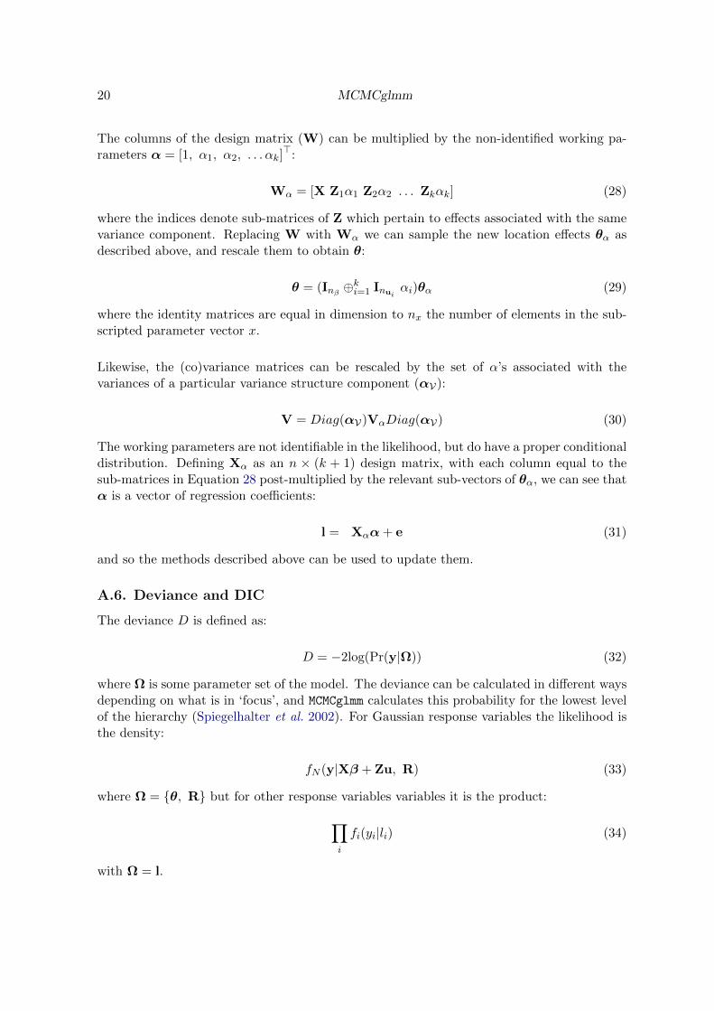
The columns of the design matrix (W) can be multiplied by the non-identified working pa-rameters α = [1, α1, α2, . . . αk]

>:

Wα = [X Z1α1 Z2α2 . . . Zkαk] (28)

where the indices denote sub-matrices of Z which pertain to effects associated with the samevariance component. Replacing W with Wα we can sample the new location effects θα asdescribed above, and rescale them to obtain θ:

θ = (Inβ ⊕ki=1 Inui

αi)θα (29)

where the identity matrices are equal in dimension to nx the number of elements in the sub-scripted parameter vector x.

Likewise, the (co)variance matrices can be rescaled by the set of α’s associated with thevariances of a particular variance structure component (αV):

V = Diag(αV)VαDiag(αV) (30)

The working parameters are not identifiable in the likelihood, but do have a proper conditionaldistribution. Defining Xα as an n × (k + 1) design matrix, with each column equal to thesub-matrices in Equation 28 post-multiplied by the relevant sub-vectors of θα, we can see thatα is a vector of regression coefficients:

l = Xαα+ e (31)

and so the methods described above can be used to update them.

A.6. Deviance and DIC

The deviance D is defined as:

D = −2log(Pr(y|Ω)) (32)

where Ω is some parameter set of the model. The deviance can be calculated in different waysdepending on what is in ‘focus’, and MCMCglmm calculates this probability for the lowest levelof the hierarchy (Spiegelhalter et al. 2002). For Gaussian response variables the likelihood isthe density:

fN (y|Xβ + Zu, R) (33)

where Ω = θ, R but for other response variables variables it is the product:∏i

fi(yi|li) (34)

with Ω = l.

Jarrod Hadfield 21

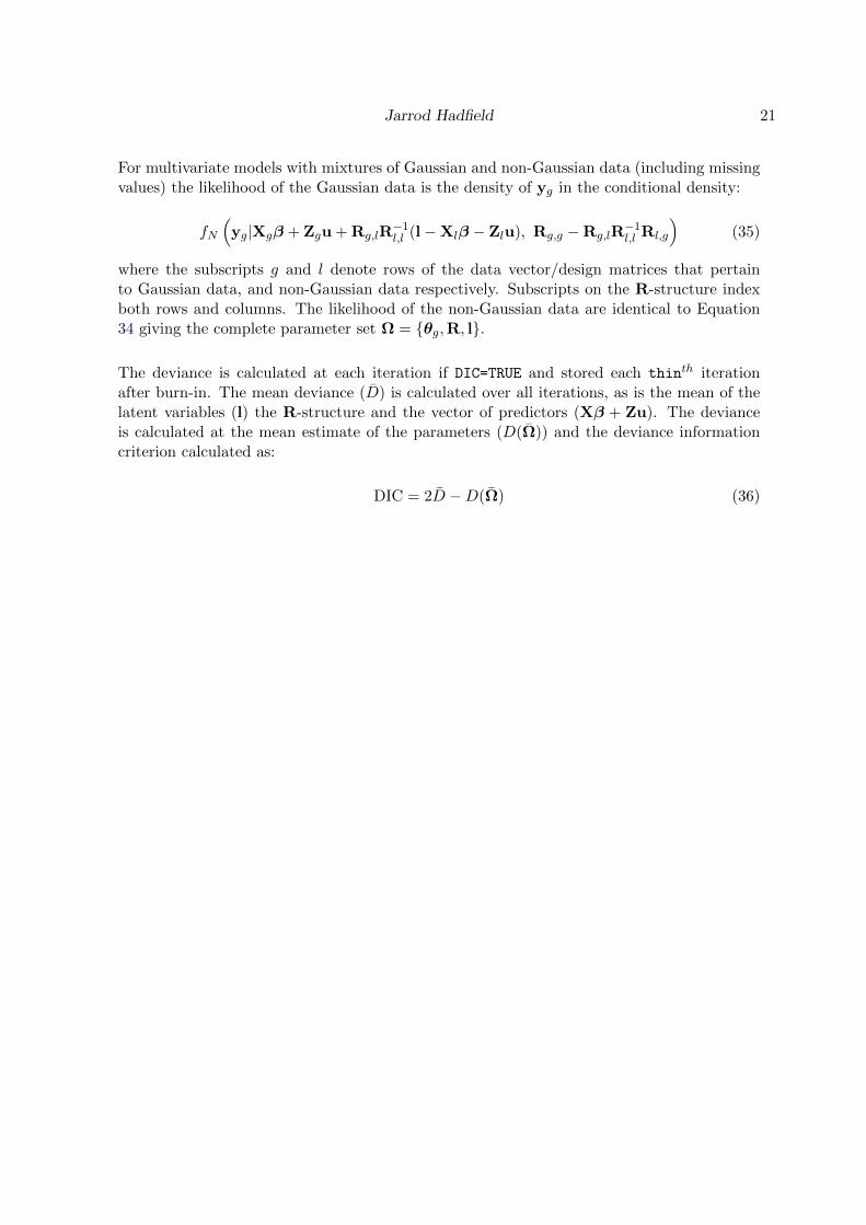
For multivariate models with mixtures of Gaussian and non-Gaussian data (including missingvalues) the likelihood of the Gaussian data is the density of yg in the conditional density:

fN

(yg|Xgβ + Zgu + Rg,lR

−1l,l (l−Xlβ − Zlu), Rg,g −Rg,lR

−1l,l Rl,g

)(35)

where the subscripts g and l denote rows of the data vector/design matrices that pertainto Gaussian data, and non-Gaussian data respectively. Subscripts on the R-structure indexboth rows and columns. The likelihood of the non-Gaussian data are identical to Equation34 giving the complete parameter set Ω = θg,R, l.

The deviance is calculated at each iteration if DIC=TRUE and stored each thinth iterationafter burn-in. The mean deviance (D) is calculated over all iterations, as is the mean of thelatent variables (l) the R-structure and the vector of predictors (Xβ + Zu). The devianceis calculated at the mean estimate of the parameters (D(Ω)) and the deviance informationcriterion calculated as:

DIC = 2D −D(Ω) (36)

22 MCMCglmm

Dis

trib

uti

onN

o.D

ata

No.

late

nt

Den

sity

funct

ion

typ

eco

lum

ns

colu

mns

"gaussian"

11

Pr(y)

=f N

(wθ,σ

2 e)

"poisson"

11

Pr(y)

=f P

(exp(l

))

"categorical"

1J

-1Pr(y

=k|k6=

1)=

exp(lk)

1+∑ J−

1j=1

exp(lj)

Pr(y

=1)

=1

1+∑ J−

1j=1

exp(lj)

"multinomialJ"

JJ

-1Pr(y k

=nk|k6=J

)=

(ex

p(lk)

1+∑ J−

1j=1

exp(lj)

) n kPr(y k

=nk|k

=J

)=

(1

1+∑ J−

1j=1

exp(lj)

) n k"ordinal"

11

Pr(y

=k)

=FN

(γk|l,

1)−FN

(γk−1|l,

1)

"exponential"

11

Pr(y)

=f E

(exp(−l)

)

"geometric"

11

Pr(y)

=f G

(ex

p(l)

1+

exp(l))

"cengaussian"

21

Pr(y 1>y>y 2

)=

FN

(y2|wθ,σ

2 e)−FN

(y1|wθ,σ

2 e)

"cenpoisson"

21

Pr(y 1>y>y 2

)=

FP

(y2|l)−FP

(y1|l)

"cenexponential"

21

Pr(y 1>y>y 2

)=

FE

(y2|l)−FE

(y1|l)

"zipoisson"

12

Pr(y

=0)

=ex

p(l2)

1+

exp(l2)

+( 1−

exp(l2)

1+

exp(l2)

) f P(y|e

xp(l1))

Pr(y|y>

0)=

( 1−

exp(l2)

1+

exp(l2)

) f P(y|e

xp(l1))

Jarrod Hadfield 23

"ztpoisson"

11

Pr(y)

=fP(y|e

xp(l))

1−fP(0|e

xp(l))

"hupoisson"

12

Pr(y

=0)

=ex

p(l2)

1+

exp(l2)

Pr(y|y>

0)=

( 1−

exp(l2)

1+

exp(l2)

) f P(y|e

xp(l1))

1−fP(0|e

xp(l1))

"zapoisson"

12

Pr(y

=0)

=1−

exp(e

xp(l2))

Pr(y|y>

0)=

exp

(exp(l2))

fP(y|e

xp(l1))

1−fP(0|e

xp(l1))

"zibinomial"

22

Pr(y 1

=0)

=ex

p(l2)

1+

exp(l2)

+( 1−

exp(l2)

1+

exp(l2)

) f B(0,n

=y 1

+y 2|

exp(l1)

1+

exp(l1))

Pr(y 1|y

1>

0)=

( 1−

exp(l2)

1+

exp(l2)

) f B(y

1,n

=y 1

+y 2|

exp(l1)

1+

exp(l1))

Table

2:

Dis

trib

uti

onty

pes

that

can

fitt

edusi

ngMCMCglmm.

The

pre

fixes

"zi","zt","hu"

and"za"

stan

dfo

rze

ro-i

nfl

ated

,ze

ro-t

runca

ted

,hurd

lean

dze

ro-a

lter

edre

spec

tive

ly.

The

pre

fix"cen"

stan

dard

sfo

rce

nso

red

wh

erey 1

andy 2

are

the

upp

eran

dlo

wer

bou

nd

sfo

rth

eunob

serv

eddatu

my.J

stan

ds

for

the

num

ber

ofca

tego

ries

inth

em

ult

inom

ial/

cate

gori

cal

dis

trib

uti

ons

and

this

mu

stb

esp

ecifi

edin

the

fam

ily

argu

men

tfo

rth

em

ult

inom

iald

istr

ibuti

on

.T

he

den

sity

funct

ion

isfo

ra

singl

edat

um

ina

un

ivar

iate

model

wit

hw

bei

ng

aro

wve

ctor

ofW

.f

andF

are

the

den

sity

and

dis

trib

uti

onfu

nct

ions

for

the

sub

scri

pte

ddis

trib

uti

on

(N=

Norm

al,P

=P

ois

son,E

=E

xp

onen

tial

,G

=G

eom

etri

c,B

=B

inom

ial)

.T

heJ−

1γ

’sin

the

ord

inal

mod

els

are

the

cutp

oin

ts,

wit

hγ1

set

toze

ro.

24 MCMCglmm

Affiliation:

Jarrod HadfieldThe EGIDepartment of ZoologyUniversity of OxfordOxford, OX1 3PS, UKE-mail: jarrod.hadfield@zoo.ox.ac.ukURL: http://www.zoo.ox.ac.uk/egi/people/researchfellows/jarrod_harrod.htm

Jarrod Hadfield 25

Syntax

nC

ovar

iance

Cor

rela

tion

rfactor

1

VV

VV

VV

VV

V

1

11

11

11

11

us(ffactor):rfactor

6

V1,1

V1,2

V1,3

V1,2

V2,2

V2,3

V1,3

C2,3

V3,3

1

r 1,2

r 1,3

r 1,2

1r 2,3

r 1,3

r 2,3

1

ffactor:rfactor

1

V0

00

V0

00

V

1

00

01

00

01

rfactor+ffactor:rfactor

2

V1

+V2

V1

V1

V1

V1

+V2

V1

V1

V1

V1

+V2

1

rr

r1

rr

r1

†

idh(ffactor):rfactor

3

V1,1

00

0V2,2

00

0V3,3

1

00

01

00

01

Table

3:

Diff

eren

tra

ndom

effec

tsp

ecifi

cati

ons

wher

effactor

isa

fact

orw

ith

thre

ele

vels

an

drfactor

isa

fact

or

wit

h(u

sually)

many

leve

ls.

The

resu

ltin

g3×

3co

vari

ance

and

corr

elat

ion

mat

rice

sof

rfactor

effec

tsw

ithin

and

acr

oss

ffactor

fact

orle

vels

are

give

n,

toge

ther

wit

hth

enum

ber

of

para

met

ers

tob

ees

tim

ated

(n).

Con

tinuou

sva

riab

les

can

also

gow

ithin

the

vari

ance

stru

cture

funct

ions

(e.g

.,us,idh).

Inth

isca

seth

eas

soci

ated

par

amet

ers

are

regr

essi

onco

effici

ents

for

wh

ich

(co)v

aria

nce

sar

ees

tim

ate

d.†

:rR

>0