Matrix functions and applications

Part II—Functions of a matrix

In Part II of this series, differential equations with constant matrix coefficients are introduced. These equations may be solved explicitly by finding the eigenvalues and by expressing the junctions of a diagonal matrix in terms of its constituent idempotents

J. S. Frame Michigan State university

2.1 M a t r i x d i f ferent ia l equat ions The matrix equat ions

dX -—= AX dt

Χ(ΰ)

x(m = c

dX\

(2.1.1)

= V (2.1.2)

in which A and ^ are Λ X M constant matrices and X, C, F a r e /2 X 1.column vectors, provide a simplified nota­tion for the two systems of η linear diff*erential equat ions in the η unknowns Xu . . . , Xn:

dxi

ώ ^ 1^ """'^' 1 = 1,2, . . . . η (2.1.3) Η

+ Σ ^^^^^ = ^ / = 1, 2, . . . , /I (2.1.4) dt^ J = i

Solutions in the one-dimensional case would be, respec­tively,

X = e'^^C

X = (cos B^^^t)C φ / s i n 5 i / 2 A

(2.1.5)

(2.1.6)

It is natural to try to define such functions as e^^ B^^^, cos B^^-^t, when A and B a r e square matrices, so that (2.1.5) and (2.1.6) will give the solutions in the general AI-dimensional case. We shall seek a closed expression for a n analytic function f(A) of a square matrix A in terms of corresponding functions of scalars.

2.2 L inear t rans format ions a n d m a t r i x eigenvectors a n d eigenvalues

An η X η matrix A maps each η X 1 column vector X into an image vector AX. A mapping in which scalar multiples and sums of vectors are mapped into corre­sponding scalar multiples and sums of their image vectors is called a linear t ransformation. A change from old coordinates X t o new coordinates Y for the same vector may be specified by any nonsingular η X η matrix S by setting

SY S-'X (2.2.1)

A corresponding change must then be made in the matrix A tha t describes the linear t ransformation X -^ AX. Since the t ransformation is linear, it maps S^^ X into S^^AX. Expressed in the new coordinate system, this is written

Y-^S-'ASY whenever X-> AX and X = SY (2.2.2)

102 IEEE s p e c t r u m A P R I L 1964

The new matrix for the linear t ransformation is S^^AS. Among the simplest to describe is a linear t ransformation that in some suitable coordinate system is represented by a diagonal matrix Λ = S~^AS with diagonal entries denoted by λι, λο, . . . , λ». It simply multiplies the newyth coordinate vector U.j (represented in the old coordinates as theyth column S.j of S) by the scalar λ/, for all y, and maps the linear combinat ions of these so-called eigen­vectors into corresponding linear combinat ions of their images.

Corresponding facts hold for the linear t ransformation of the row vectors Z ^ , which are defined by the mapping Z'^-^Z'^A.

Definition 2.2.1 A nonzero column vector X (or row vector Z ^ ) , that is mapped by an η X η matrix A into a scalar multiple λΧ (or λ Ζ Ο of itself, is called a column (or row) eigenvector of A. The corresponding scalar λ is called an eigenvalue of A. Condi t ions that the nonzero column vector X be an eigenvector of A may be written as follows:

AX = X\ or (\U - A)X = 0 (2.2.3)

Corresponding condit ions for a row eigenvector Z^ 9^ 0 are

Z'^A = λ Ζ ^ or Z^\\U - A) = 0 (2.2.4)

Each of the two systems of η equat ions in η unknowns has the solution vector 0. The vanishing of the deter­minant of the coefficient matrix XU — A, called the characteristic matrix of A, is a necessary and sufficient condition for the existence of nonzero solutions that de­termine a column eigenvector X by (2.2.3) or a row eigen­vector Z ^ by (2.2.4). This determinant D{\) is called the characteristic polynomial of A. It is the following monic polynomial of degree n:

D(\) = \\ϋ - A\ (2.2.5)

= λ'̂ + d.X^-' + d^n-^ φ . . . φ dn-i\ + dn

π (λ - λ,)^ 3 = 1

(2.2.6)

The characteristic equation D(\) = 0 has characteristic roots Xj, with characteristic multiplicities nj, that are the η eigenvalues of A. The set σ(Α) of these η eigenvalues, including repetitions, is called the spectrum of A. Their product is the determinant of A and their sum is its trace

Ml = Π λ Λ = (~ l )Vn (2.2.7)

η a

trA=^ ^ a u = = -di (2.2.8) t=i y=i

To each of the s distinct eigenvalues Xj of A there corre­sponds at least one eigenvector X 9^ 0 that satisfies (2.2.3), or Z^ 9^ 0 that satisfies (2.2.4). When all a/eigen­values of A are distinct, the corresponding η eigenvectors X constitute the columns S,j of a matrix 5 , and the eigenvalues are diagonal entries of a matrix Λ such that AS = .SA. If S is nonsingular this implies Λ = S^AS,

Example I F ind the eigenvalues and eigenvectors of the matrix

^ 1 2" 4 3

Solution:

D(X) = \XU- A\

= (λ - 1)(λ - 3) - 8

λ - 1 - 2 - 4 λ - 3

= λ2 - 4λ - 5

= (λ + 1)(λ - 5) (2.2.9)

IEEE spectrum april 1964 103

Thus the eigenvalues of are λι = — 1, λ2 = 5. Their sum is tr ^ = 1 + 3 = 4 and their product is | ̂ | = 3 - 8 = - 5 . Solution vectors X for (λ^ί/ - A)X = 0 are the eigenvectors S.^.

( - 1 - 1) - 2 - 4 ( - 1 - 3 ) J

S,i

(5 - 1) - 2 . - 4 ( 5 - 3 ) J

1̂ X2j

1̂

a —a

b

lb

for any α ? i 0 (2.2.10)

for any b ^ ^

Taking a = b = 1, we form the matrix S = {S.uS.i) and the diagonal matrix Λ with diagonal entries λι, λ^.

(2.2.11) 1 Γ " - 1 0"

Λ = 0 5_

"1 2" 1 Γ " - 1 5" - 4 3_ 2_ 1 I O _

1 Γ • - 1 0" . - 1 2 . 0 5_ SK. (2.2.12)

Definition 2.2.2 Fo r any nonsingular matrix 5 , the matr ix S'^AS is said to be similar t o ^ .

Definition 2.2.3 A matrix is called diagonable if it is similar to a diagonal matrix.

Clearly, similarity is a reflexive, symmetric, and transi­tive relation tha t divides all λ X /i matrices into mutually exclusive classes of similar matrices, each representing the same hnear t ransformation in an appropr ia te co­ordinate system. F o r each class of similar matrices there a re impor tan t c o m m o n properties. F o r each class there a re certain "spec t ra l " matrices that are considered to be the simplest for describing the corresponding linear t ransformation. Fo r a diagonable matrix A the spectral matr ix is a diagonal matrix with the same eigenvalues.

Fo r example, the matrices

1 2 4 3 and Λ =

- 1 0" 0 5

in (2.2.12) are similar. A is diagonable and Λ is its spec­tral matrix.

Theorem 2.2.1 Two similar square matrices have the same characteristic polynomial .

Proof: Since the determinant of the product of two square matrices equals the product of their determinants , we have

\\U - S-^AS\ = \S-^\ \\S - AS\

= | λ 5 - ^ 5 | | 5 - ι |

= \\U - A\ = D{\) (2.2.13)

It follows that any two similar matrices A and S'^AS have the same eigenvalues with the same characteristic multiplicities Hj and hence the same trace and determi­nant . They also have the same rank. Fo r example, the following 5 X 5 matr ix A is similar t o the upper t r i ­angular matr ix S'^AS = Γ.

"1 0 0 0 0" " 3 2 3 0 - 3 " 1 1 0 0 0 1 - 1 - 2 1 4 1 0 1 0 0 2 - 2 - 2 2 5 1 0 0 1 0 - 2 - 2 - 3 - 2 6

_1 0 0 0 I j - 5 - 2 - 3 0 1 5 - 1 A

" 1 2 3 0 - 3 " 0 1 1 1 1

= 0 0 1 2 2 0 0 0 - 2 3 0 0 0 0 - 2

= Τ

0 0 0 0 ' 1 0 0 0 0 1 0 0 0 0 1 0 0 0 0 1

(2.2.14)

No te that A and Γ both have trace — 1 and determinant 4. However, if multiple roots are present, two η X η mat­rices with the same spectrum are not necessarily similar.

2.3 S i m i l a r i t y t o t r i a n g u l a r a n d spectral mat r ices Eigenvalues of a tr iangular matr ix can be determined

by inspection. Theorem 2.3.1 The eigenvalues of an λ X λ t r iangular

matr ix are its η diagonal entries. Proof: If Τ is any η X η t r iangular matrix (upper tri­

angular , lower tr iangular, or diagonal) then the matrix \U — Τ is also tr iangular, so its determinant D(X) is the product

Π ( λ - tjj)

of its diagonal entries λ — tjj. Hence tjj are the eigen­values \j of T,

Definition 2.3.1 A triangular matrix is simply ordered if equal eigenvalues appear next to each other along its diagonal. The matr ix Τ in (2.2.14) is a simply ordered upper tr iangular matrix with a triple eigenvalue 1 and a double eigenvalue —2. A Jacobi matrix is a simply ordered upper tr iangular matrix whose ij entry is zero whenever the /th and yth diagonal entries are distinct (λί 7̂ A Jacobi matrix is a quasi-diagonal direct sum of s blocks of respective dimensions /ij, each block being an upper tr iangular matrix with equal eigenvalues.

The following Jacobi matrix Ji and Jordan matrix Λ are each similar to the upper triangular matrix Τ in (2.2.14):

Ji =

1 2 3 0 O i l 0 0 0 1 0 0 0 0 - 2 0 0 0

0" 0 0 3

0 - 2

" 1 1 0 0 O i l 0 0 0 1 0 0 0 0 - 2 0 0 0

0" 0 0 1

0 - 2 .

Definition 2.3.2 A Jordan matrix Λ is a Jacobi matrix whose ij entries are 0 unless j = / or / + 1. Its (/, / + 1) entry may be 0 or 1 if λί = λ^+ι, but is 0 otherwise. A Jordan matrix is the direct sum of one or more simple Jordan matrices each having equal eigenvalues on its diagonal, I's immediately to the right of the diagonal, and O's elsewhere.

A =

AiO . . . 0 0 A 2 . . . 0

0 0 . . . Λ J

J o r d a n

"λ, 1 0 . . . 0 0 0 1 . . . 0 0

ο 0 0 . . . λ^Ι LO ο ο . . . ο J

S i m p l e J o r d a n

(2.3.1)

104 IEEE spectrum A P R I L 1964

A Jordan matrix Λ is a diagonal matrix if and only if all its simple Jo rdan submatrices are one-dimensional . A diagonable matr ix may have repeated eigenvalues.

We shall prove tha t every η X η matrix is similar to a n upper tr iangular matrix, indicate that it is similar to a Jacobi matrix, and merely state that it is similar to a Jordan matrix. The latter will be called its spectral matrix.

Definition 2.3.3 A matrix S is called unitary if

5 5 * = 5 * 5 = t / (with 5 unitary) (2.3.2)

where 5 * denotes the conjugate t ranspose of 5 . The product of two η X η unitary matrices is easily

shown to be unitary. If 5 is unitary, the matrix A is called unitarily similar to S*AS or to 5/45*. It is easier to per­form a unitary change of coordinates, for which 5~^ = 5* , than one in which the computa t ion of 5~^ is more complicated.

Theorem 2.3.2 Any nXn matrix A is unitarily similar to an upper tr iangular matr ix Τ whose diagonal entries are the eigenvalues of A a r ranged in any prescribed order. Tha t is,

A = 5 Γ 5 * (2.3.3)

where 5 5 * = i/, Γ is upper tr iangular, and tjj = λ^. Proof: Since any 1 X 1 matrix is itself upper tri­

angular , the theorem is t rue for Λ = 1 with 5 = t/i = 1. T o prove the theorem by mathematical induction, we as­sume its validity for square matrices of order less than n, and prove it for an arbi t rary nXn matrix A whose eigen­values have been numbered in the prescribed order λι, λ2, . . . , λη, (allowing repetitions). An eigenvector of A for the eigenvalue λι is first reduced to a unit vector by divid­ing by its length; then its first component is changed to a real number χ > 0 , by dividing the vector (if necessary) by a complex number of absolute value 1 tha t preserves the length. F r o m the part i t ioned unit eigenvector

1 row

7 2 — 1 rows

we construct the η X /i matr ix

lX\-U + XX*/(\+x)]

(2.3.4)

F I * F I = x^ + X*X = 1

Direct multiplication shows that V is not only hermitian (V = K*), but also uni tary :

VV* = y*y = Un V2*V, = 0

Since AV^ = FiXi, the t ransform of A by V is

K,* K.>*

λ, V,*AV2 0 V^^AV^

(2.3.5)

(2.3.6)

Since A and V*AV have equal eigenvalues, those of V'i*AV^> are λ,., . . . λη. By induction hypothesis the (/2 — 1) X (A7 — 1) matrix V2*AV2 can be transformed into an upper tr iangular matrix T2 with diagonal entries XI, . . . , λη, by means of a unitary matr ix IV.

W%V2*AV2)]V ^ Γ2(uppertriangular)

Construct the unitary matr ix 5 such tha t

"1 0

W*W=^ Un-l

(2.3.7)

0 W (Vi, ViW) SS* = U (2.3.8)

S*AS 1 0 ' 0 W* V*AV\

1 0 ' 0 W

λι Vi*AV2fV' 0 Γ2

(2.3.9)

Then Τ is the required upper tr iangular matr ix, unitarily similar t o A.

Definition 2.3.4 A matrix A is called normal if AA* = A* A. The class of normal matrices includes hermitian and real symmetric matrices, uni tary and real or thogonal matrices, real skew matrices, and several other impor tan t types.

The following normal matrices are marked V if uni­tary (KK* = U), if̂ if real or thogonal (ίΤΗ^^ = U),Hif hermitian (H = / / * ) , 5 if real symmetric ( 5 = 5^0, ^ i f real skew (K = -AT^), and Ε if idempotent (E^ = E):

Lv

V3 Va Va Va - Va Va

Va - V a J

0 Γ - 1 0

V, W, H, S V, w, κ

• M l + 0 V. ( i + if . - • M l + 0 ' M l - 0.

V Η, Ε

Theorem 2.3.3 Every normal matr ix A is unitarily similar to a diagonal matrix.

Proof: If A is normal , so is the upper tr iangular matrix Τ = 5 * / ί 5 of (2.3.9), since

7 T * = S''ASS''A*S = 5*/4/4*5 = S*A*AS = T*T

(2.3.10)

The squared lengths of the yth row and jth column of Τ must be equal , since these are the yth diagonal entries of 7 T * and T*T, respectively. Applied successively for j = 1, 2, 3, . . . , w — 1, this condit ion requires that all entries of Τ t o the right of the diagonal must vanish. Τ is diagonal and the theorem is proved.

The matrix equat ion

λ,· Cjk 0 λ^

1 cj,/{\, - λ,)

0 1 1 cj,/(\k - \

0 1 Ίο' y (2.3.11)

suggests a proof of the fact that every simply ordered up­per tr iangular matrix can be transformed into a similar Jacobi matrix by reducing to zero each jk entry for which

9^ λ, . Stated here without proof is the impor tant fact (to be

discussed in Par t IV) that every Jacobi matrix, and hence every square matrix, is similar to a Jo rdan matrix. The eigenvalues λ^, and the dimensions of the one or more simple Jo rdan blocks for each λ/, constitute a complete set of invariants for a class of similar matrices, that are completely determined by the ranks of the matrices (XjU — A) and their powers.

Definition 2.3.5 A Jo rdan matrix Λ = S'^AS that is similar to a given matrix A is called a spectral matrix for A, and the transforming matr ix 5 with modal columns S.j is called a right modal matrix for A. Its inverse, R = 5 ~ ^ with moda l rows Rf, is called a left modal matrix for A,

Fur ther discussion of nondiagonable matrices will be postponed to Par t IV. The rest of the present discussion

IEEE spectrum A P R I L 1964 105

will be devoted to diagonable matr ices—that is, those whose spectral matrices are diagonal .

2.4 F u n c l i o n s off d iagonable mat r ices The equat ions

AS = SA or A = SAS'^ (2.4.1)

satisfied by any two similar matrices A and Λ imply the relations

A^S = ASA = S A 2 or A^^S = 5Λ* A: = 1 , 2 , 3 , . . .

(2.4.2)

Hence if / (λ) and f'(A) denote corresponding scalar and matrix polynomials

/ ( λ ) = /ολ^' + / , λ - - ι + + . . . + Λ . Λ + fm

(2.4.3)

f(A) = foA'' - f Μ^^-' + M'^-'' + . . . + fm-iA + J^U

(2.4.4)

then by addit ion using (2.4.2) we find

f(A)S = Sf(A) f(A) = Sf(A)S-^ (2.4.5)

Under this correspondence, sums and products of functions of Λ are mapped into corresponding sums and products of functions of ^ . If for the spectral matr ix A such functions as cos A^'H, . . . can be defined uniquely, then (2.4.5) defines the corresponding functions of A.

Let A = S~^AS be a diagonal matrix similar to a given diagonable matrix A, Then for any polynomial / ( λ ) we have

/ ( Λ ) =

0 / ( λ Ο

Ο Ο

Ο

Ο η

Χ^/(λ,)€.. (2.4.6)

where en are the matrix units defined in Part I. An important special case is th is : Theorem 2.4.1 (Hamilton-Cayley theorem) Every

square matrix satisfies its characteristic equat ion. Proof for diagonable matrices: Taking Ζ)(λ) lor fiX)

in (2.4.6), it follows that D(\) = 0 for each,/ , so D{A) is the zero matrix. By (2.4.5) it follows that D{A) is also the zero matrix.

Example 2 Taking A as in Example 1, we have

9 8" .16 17

Ό 0" 0 0

- 4 1 2 4 3 - 5

1 0" 0 1

(2.4.7)

Definition 2.4.1 A matrix Ε is called idempotent if Ε = ΕΚ Examples of 2 X 2 idempotent matrices are

Ί 0 ' 0 0 ' Va - V e '

. 0 0 . . 0 1 . . 7 3 V s . . - V 3 V s .

The first two of these are diagonal idempotents . Both the first pair and second pair have sum U and product 0.

Equat ions (2.4.6) and (2.4.5) may be used t o define

/ (A) and / ( /4 ) , if/(X) is a function defined by a power series tha t converges at all the eigenvalues of A (or of A).

If A has the s distinct eigenvalues with respective multiplicities nj, we shall denote by Ij the sum of the nj matrix units en for all / such tha t λί = \j. This matrix Ij is a diagonal idempotent matrix with nj I ' s as diagonal entries, and having rank and trace nj. I ts transform by S is a so-called constituent idempotent matrix Aj for A, whose rank and trace are also nj.

for λί =

(2.4.8)

The idempotents Ij and Aj satisfy the relations

= Y^A, = U (2.4.9)

Ijh = hhk AjA, = Ajbjic (2.4.10)

Theorem 2.4.2 An analytic function of a diagonable matrix A, whh distinct eigenvalues λ^, where y = 1,2, . . . s, and corresponding consti tuent idempotent matrices Aj defined by (2.4.8), is expressed by the equation

8 (2.4.11)

Proof: On transforming/(A) in (2.4.6) by S and apply­ing (2.4.8) we obtain the required resul t :

f(A) = Sf(A)R = ^fiXdSeuR (2.4.12) t = l

Thus any analytic function of a diagonable matrix A that has s distinct eigenvalues \j (of multiplicities nj) is a linear combinat ion of the s constituent matrices Aj, The power formula

A'' 8

(2.4.13)

can also be used for A: = —1 to compute the inverse A~^ of a matrix A without 0 eigenvalues, since

8 8 λ,Α,- ^ Xr'An

i = l Λ = 1

j,h λ/» j

For nonintegral values of k, the function /i* may be multi­ple valued.

T o use (2.4.11), the eigenvalues and corresponding constituent idempotents Aj must first be computed. The former are roots of the characteristic equat ion D(\) = 0. The latter can be computed from the modal matrix S and its inverse R if these are known. Fo r normal matrices A, such tha t A A* = A* A, including real symmetric or real or thogonal matrices, the modal matrix S may be chosen unitary, so that R =^ S'^ = S* and Ri, = S,i*, Here the eigenvectors S.j suffice to determine the constituent idempotents from (2.4.8).

However, the constituent idempotents Aj can be de­termined directly as polynomials in A by (2.4.18), without knowing the eigenvectors. The columns of Aj can then

106 IEEE spectrum A P R I L 1964

be used to compute the eigenvectors. T o show this, we choose for / ( λ ) in (2.4.6) the interpolatory polynomial q^(X) of degree 5 — 1 defined by

λ - λ,

^ • = 1 — Xj (2.4.15)

We note tha t qk(X) vanishes at each root except λ^.

gjcih) = 0 k q,(X,) = 1 (2.4.16)

Hence

^.(Λ) = h (2.4.17)

A - \jU A, = ShR = q,iA) = Π . .

•̂ = 1 ΛΑ —

(2.4.18)

Here then is an explicit formula for the consti tuent idempotents of a diagonable matr ix A. In Example 1 (Section 2.2), where λι = — 1 and Λ2 = 5, we have

A = 1 2

4 3 Al =

A - 5U _ 5U - A

- 1 - 5 " 6

V3 -73 L-V3 V3J

(2.4.19)

A2 = A + U _ U φ A

5 + 1 ~ 6 V3 V:

LV3 V3J W e note tha t A^A, = 0, ^1 + ^ 2 = A^ = X iMi + Λ2Μ2, t r / l i = t r /Ί2 = 1, and tha t the columns of Ai and A2 are eigenvectors of A for the eigenvalues λι, Λ2.

Theorem 2.4.3 Eigenvectors of any square matrix that correspond to distinct eigenvalues are linearly inde­pendent .

Proof: Let λι, Λ2, . . . , λ̂ be distinct eigenvalues of an Λ X Λ matr ix A, and let the columns S.u S.2, .,S.s of ann X s matr ix S be corresponding eigenvectors. Then

AS .j = S.jXj AS = SA (2.4.20)

where Λ is an J X 5 diagonal matrix with the distinct numbers λι . . . λ, on the diagonal . Linear independence of the s vectors S.J means that if s scalars CJ form an s X 1 column vector C such that SC = 0, then C = 0. Assuming SC = 0, we multiply on the left by qj(A); see (2.4.15). Then

0 = qj(A)SC = Sqj(A)C = 5e , ,C = S.JCJ (2.4.21)

0 Since 5 .^ 5 ^ 0, we have CJ = 0 for all / Hence SC implies C = 0.

Theorem 2.4.4 If A is any normal matr ix, then there exists a polynomial / ( λ ) such that

A* = f(A) Xj* = f(Xj) for each j (2.4.22)

Proof: Since Ij = we have

•8 a

A = ^ XjAj = ^ XjSIjS* (2.4.23) i = i 3=1

8 8 8

(2.4.24)

T H E REQUIRED GOLVAQRAKL IS.

/ ( λ ) = Σ which proves (2.4.22).

Theorem 2.4.5 Every matr ix Β tha t commutes with an η X η matr ix A having η distinct eigenvalues is equal to a polynomial in A.

Proof: If Β commutes with A it commutes with the idempotents Aj = S.jRj. that are polynomials in A. Let μj = Rj.BS.j. Then

Β = UB η η 8

Σ ^̂ '̂ = Σ -̂^̂^̂ = Σ '̂-̂'̂^̂ ·̂ J=i j=l j=l

(2.4.25)

= Σ ^̂̂^ = Σ ^̂̂^̂̂^ = ̂ ^̂̂ Where / (λ ) = Σ̂^̂ <̂̂)

A word of caution is necessary in saying that all func­t ions of a diagonable matrix are expressible by Eq. (2.4.11). This equat ion evaluates single-valued analytic functions, but may not give all values of multiple-valued functions, such a s / ( λ ) = λ̂ ^̂ F o r example, the following equat ion shows that the 2 X 2 unit matrix U has infinitely many square roots that are not expressible as polynomials in U.

2 Ί ο' —

cos θ sin Θ sin Θ —cos Θ

2.5 C o m p u t a t i o n off ffunctions off matr ices

Example 3 F ind the square roots of

(2.4.26)

"8 4' 4 8 A =

Solution:

D(X) = \XU - A\

= Λ2 ~ 16λ + 48 = (λ - 4)(λ - 12)

(2.5.1)

λ - 8 - 4 1 - 4 λ - 8

The eigenvalues of A are λι = 4, Λ2 = 12. The constituent idempotents of A are

A, = ^ - Λ2<7 12U - A

λι - Λ2 8 V2 - V 2

A2 = A - XiU _ A-AU

X2 — Xi 8

Check :

Ai^ = Au Ai^ = An, AiA,

(2.5.2)

A = \\Ai + XiAi 1 - 2

- 2 2

0, / i i +

+ 6 6 6 6

The solution to the problem includes four square roots of A.

± 3 " 2 | 1 - 1

- 1 1 1 1 1 1 (2.5.3)

IEEE spectrum A P R I L 1964 107

Columns of Αι and Α·2 a re eigenvectors of the symme­tric matrix A. A unitary modal matrix S and its inverse S* are

5 = V 2 L-V2 V2J and

= S* V2 LV2 V D (2.5.4)

where we have multiplied the columns in (2.5.2) by 2"'^ t o make them of unit length.

Example 4 Evaluate e'* if

J

where 7" = - u .

Solution: DQC) \ ~\ = -|- 1

0 Γ - 1 0

where λι = j , λ·ί = = - 1 .

Const i tuent idempotents of / are

J - Xo.U J + jU U - jJ Jx =

λι - λ 2 2 / 2 -

J -Χ,υ J - jU U + jJ

1 - /

2\J I J

(2.5.6)

λ 2 - λ,

Check : 7, The solution is

-2j 2

Λ, Λ Λ

1 J

l-j I J

0 , 7ι -f Λ = U.

+ 1 /

L-7 I J

1 - i

cos Β sin ^

— sin ^ cos d (2.5.7)

Thus e*̂ ^ is a matrix that represents a rotat ion of the plane th rough the angle

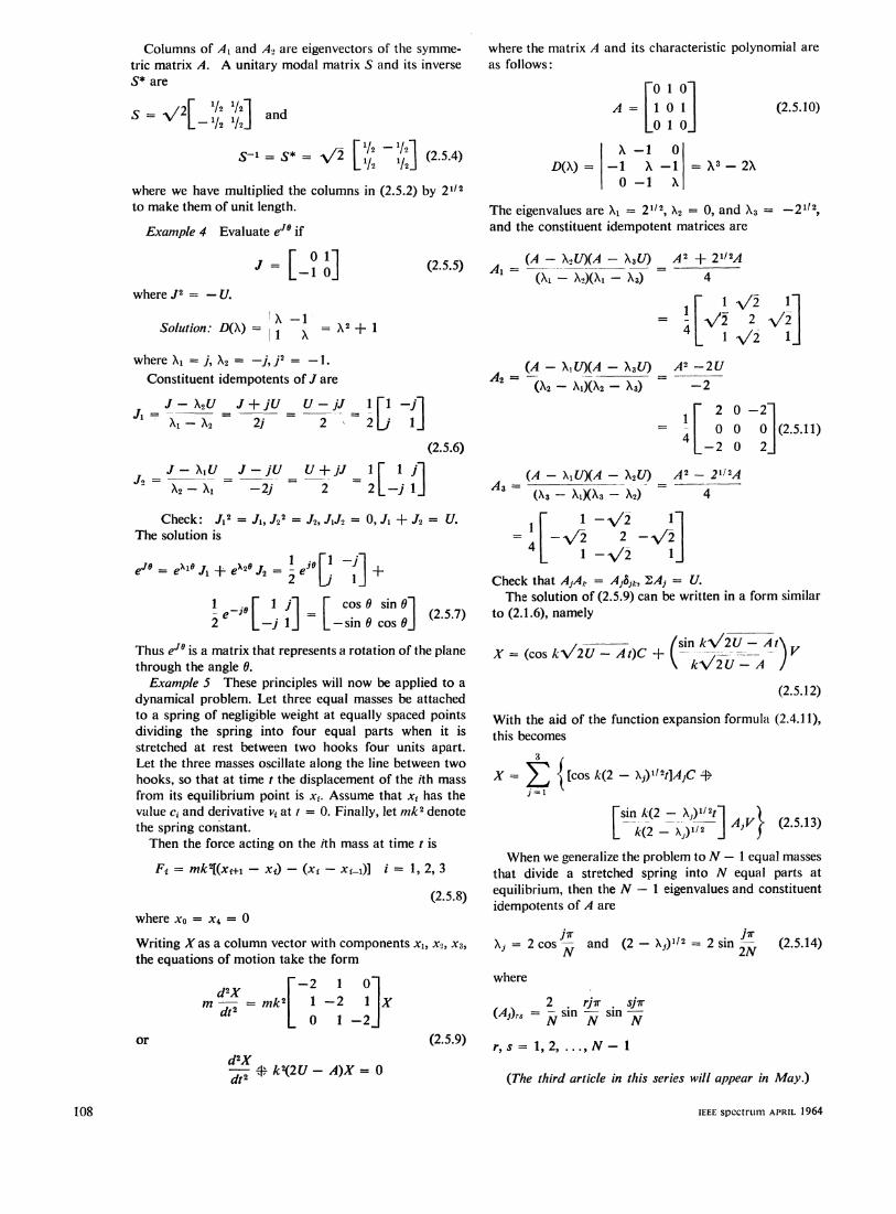
Example 5 These principles will now be applied to a dynamical problem. Let three equal masses be at tached to a spring of negligible weight at equally spaced points dividing the spring into four equal parts when it is stretched at rest between two hooks four units apar t . Let the three masses oscillate a long the line between two hooks, so that a t t ime t the displacement of the /th mass from its equil ibrium point is Xi. Assume that xi has the value d and derivative at / = 0. Finally, let mk'^ denote the spring constant .

Then the force acting on the /th mass at t ime t is

Fi = mk\(Xi+i - Xi) - (Xi ~ Xi-i)] ί

where xo = x^ = 0

1 , 2 , 3

(2.5.8)

Writ ing A' as a column vector with components Xi, x-i, Xs, the equat ions of mot ion take the form

m mk'

- 2 1 0" 1 - 2 1 0 1 - 2

or (2.5.9)

d^X — φ kHlU - A)X =0 dt^

where the matrix A and its characteristic polynomial are as follows:

0 1 0

1 0 1

0 1 0.

λ - 1 0 - 1 λ - 1

0 - 1 λ

(2.5.10)

= λ3 - 2λ

The eigenvalues are λ ι = Ι^^'^Λ^ = Ο, and XA = -2^^\ and the consti tuent idempotent matrices are

(2.5.5) A, = {A - \.U){A - \,U) _ A^ + 2''^A " ( λ ι - λ2)(λΐ - λ 3 ) " 4

• 1 V 2 1" V2 2 V 2

1 Λ / 2 1

A2 = Η (A - \iU)(A - \,U) A^ -2U

( λ 2 - λ ι ) ( λ 2 - λ 3 ) - 2

2 0 - 2 '

0 0 0 - 2 0 2

(2.5.11)

{A - liUXA - XjU) _ A" - 2 ' / M

( λ 3 - λ ,Χλ, - " λ , ) " ~ 4

1 - Λ / 2 Ι '

- V 2 2 - V 2

1 - Λ / 2 1

108

Check that AjA,: = Aj8jt, ^A, = U.

The solution of (2 .5 .9) can be written in a form similar t o ( 2 . 1 . 6 ) , namely

/ / s i n KVLU - A T\ „ Z = ( c o s . V 2 I / - ^ 0 C + ( - ^ ^ - ^ ^ - ~ ) F

( 2 . 5 . 1 2 )

With the aid of the function expansion formula (2.4.11), this becomes

3 ,

"sin A(2 - X , ) I ' 2 / T )

When we generalize the problem to TV — 1 equal masses that divide a stretched spring into equal parts at equilibrium, then the — 1 eigenvalues and constituent idempotents of A are

λ , = 2 c o s ^ ^ and (2 - X^yf^ ^ 2 ^ (2.5.14)

where

2 . r/V . sJTT (Aj)rs = ^ s m — sm — r , ^ = 1 ,2 , . . . , Λ ^ - 1

(The third article in this series will appear in May.)

IEEE s p e c t r u m A P R I L 1964