mathematical modelling of oxygen steelmaking...v abstract oxygen steelmaking is currently the...

Mathematical Modelling of Oxygen Steelmaking

Neslihan Dogan

A Thesis Presented for the Degree of Doctor of Philosophy

Mathematics Discipline

Faculty of Engineering and Industrial Sciences

Swinburne University of Technology

Melbourne, Australia

2011

iii

Declaration The candidate hereby declares that the work in this thesis, presented for the degree of

Doctor of Philosophy submitted to the Mathematics Discipline, Faculty of Engineering

and Industrial Sciences, Swinburne University of Technology; is that of the candidate

alone and has not been submitted previously, in whole or in part, in respect of any other

academic award and has not been published in any form by any other person except

where due reference is given, and has been carried out during the period from March

2007 to November 2010 under the supervision of Prof. Geoffrey Brooks and Dr. M. Akbar

Rhamdhani.

Neslihan Dogan 16 June 2011

Certification This is to certify that the above statement made by the candidate is correct to the best

of our knowledge.

Prof. Geoffrey Brooks

Dr. M. Akbar Rhamdhani

v

Abstract

Oxygen steelmaking is currently the dominant technology for producing steel from pig iron. The

process is complex because of the presence of multiple phases (liquid metal, slag, gas, etc.),

many components, and the non-steady state/non-homogenous conditions within the process. The

severe operating conditions make it difficult to take measurements and directly observe the

process. Furthermore, experimental results are not always adequate in providing an evaluation of

important parameters of the system. Mathematical modelling has been widely used to describe

the complicated nature of the process, improve understanding of the system, and optimize

process control.

Some process models have been developed to predict the temperature and carbon content of the

steel at the end of the blow. Although these models might be suitable for industrial applications

and provide reasonable approximations, existing theories have not been successfully applied to

describe the kinetics of oxygen steelmaking under dynamic process conditions. Moreover, some

recent findings on the kinetics of steelmaking were not included in these models. An example of

this is the bloated droplet theory. There is evidence that the residence time of droplets ejected

from the liquid metal to the slag-metal-gas emulsion is a strong function of the bloating behavior

of metal droplets. Recent studies have shown that the period when the bloated droplets are

suspended in the emulsion phase enhances the reaction areas, and the decarburization rates. In

this study a computer based model has been developed that incorporates bloated droplet theory

under dynamic conditions to evaluate its influence on the overall kinetics of the process. The

dynamic simulation model predicts the metal analysis for each time step throughout the blow to

provide greater control, and as a tool to optimize the steelmaking process.

In this study the process variables influencing the decarburization reaction kinetics considered in

the model were hot metal, scrap and flux charges, hot metal, scrap and slag compositions,

oxygen blowing conditions such as lance height, gas flow rates, temperature of the bath, flux

dissolution, scrap melting, ejected metal droplets behavior such as the droplet generation rate,

droplet size, residence time in the emulsion, and decarburization rates in the emulsion and

impact zones. The model did not consider the refining reactions of other impurities in the liquid

metal, the heat balance of the process, variation in slag foaming, and dissolution of the

refractories into the slag phase. Moreover, the model has been performed based on an

assumption of homogenous slag and constant slag foam height. The major limitation of this study

is that slag formation is not included. Accordingly, the amount of major metal oxides such as FeO

vi

and SiO2 present in the slag were taken from industrial data with respect to blowing time, and

were entered as input for model calculations.

All the selected process variables were modelled individually. The equations involved in this

model were solved numerically on the basis of parameters encountered in the operation of

oxygen steelmaking furnaces. Each sub-model was translated into computational code.

Accordingly, each proposed sub-model prediction was compared with the industrial or

experimental data available in the open literature. All the developed models were linked to one

another in this study. The global model was tested with actual data for a 200 t top-blown furnace

under the full scale operating conditions available in the open literature. The model was based

on a stepwise calculation of carbon removal reaction which allowed for a continuous calculation

of the change of carbon in liquid iron throughout the oxygen steelmaking process.

The model predictions proved that the carbon content of liquid iron agreed with with the actual

process data. The model suggests that 45% of total carbon was removed via emulsified metal

droplets and the remainder was removed from the impact zone during the entire blow. It was

found that the residence time of droplets and the decarburization reaction rate via emulsified

droplets, was a strong function of the bloating behavior of the droplets. The estimated residence

times of the metal droplets in the emulsion were between 0.4 and 45 seconds throughout the

blow. The values of residence time decreased towards the end of the blow because the metal

droplets became dense and were suspended for shorter times in the slag-metal-gas emulsion.

The calculations showed that the height of the lance is an important process variable to

determine the amount of metal droplets generated. A decrease in the lance height increased the

number of droplets generated and thereby increased the refining rate of carbon from liquid metal

through the emulsion phase. For example, the decarburization rates via emulsified droplets

increased from 102.7 kg/min to 222 kg/min when the lance height decreased from 2.5 m to 2.2

m.

The global model enabled a comparison of the decarburization rates in different reaction zones

and provided a better understanding of the process variables affecting in each reaction zone. On

the basis of this model, the decarburization rates in the emulsion phase reached 60% of the

overall decarburization rate during the main blow. This increase in the decarburization rates was

due to an increase in the number of droplets with long residence times in the emulsion phase.

This finding emphasizes the importance of the bloated droplet theory in predicting droplet

behavior and giving a better understanding of decarburization during the entire blow.

vii

The results of the present work can be used quantitatively to explain the phenomena occurring in

the real system and gain a better understanding of the process. These findings will provide a

further theoretical understanding of the oxygen steelmaking process and provide a predictive tool

for industrial applications. In particular, the model developed in this study allows for the

decarburization kinetics in the impact zone to be predicted separately from the decarburization

kinetics of the emulsion. This development represents an original contribution to our

understanding of steelmaking.

ix

Acknowledgments

PhD is an exciting and simulating journey but also at times challenging. Many people have

contributed to my journey in innumerable ways and I am greatful to all of them. Firstly, I would

like to express my sincere gratitude to Professor Geoffrey Brooks for the opportunity to work on

this project and for his advice during the progress of this work. His continuous energy and

enthusiasm in research motivated all his advisees, including me. In addition, he was always

accessible and willing to help his students with their research. From the very beginning he had

confidence in my ability to complete my degree. He provided me with direction and technical

support, and ultimately became more of a mentor and friend than a professor.

I gratefully thank my second supervisor Dr. Muhammad Akbar Rhamdhani for his continual

encouragement and enthusiasm to see this project completed. His guidance and valuable

suggestions are very much appreciated. I consider it fortunate to have worked with my

supervisors and been a part of the research group they created. I have learned research culture

and been well trained by my supervisors from the beginning to the final level of my degree. I

have found my research topic throughout the program to be simulating and thoughtful, providing

me with tools to explore both past and present ideas and issues.

I would like to thank Dr. Carlos Cicutti from the Centre for Industrial Research at Tenaris,

Argentina for his valuable discussions and contributions to the operational data used in this study.

It was a great moment to meet with him at the AISTech Conference 2010.

Thanks to members of the High Temperature Processing Group of the Faculty of Engineering and

Industrial Science for their ongoing support, good humour, and proof reading ability. These

current and former group members are (no special order): Winny Wulandari, Bernard Xu, Morshed

Alam, Nazmul Huda, Behrooz Fateh, Francesco Pignatale, Reiza Zakia Mukhlis and Abdul Khaliq. It

has been a great journey with them. I really enjoyed sharing experiences and knowledge in the

coffee breaks during the time of this study, particularly with Winny, Morshed, and Nazmul.

I wish to thank all of my friends outside the Department for bearing with me and their

understanding. I offer my regards and blessings to Mehrnaz Amidi, Nada Gafayri, Nadia Gafayri

and Aylin Gumus who supported me when it was most required, during the completion of the

project. Many thanks to you girls for all the fun we had in the last four years. I enjoyed every

moment of the sleepless nights we worked together Mehrnaz! My special thanks to the Sirin

x

Family, Leyla, Huseyin, and their children who treated me as a member of their family in

Australia. They gave me strength to stand for who I am.

Above all, this thesis is dedicated to my beloved parents, Mehmet and Ayfer, and my brother,

Ismet. They have given up many things for me to stand where I am standing now. They always

encouraged me and helped me pursue my dreams. They have cherished every moment and

supported me whenever I needed it. I would have not finished this work without their faith in me.

Their unconditional love and continual support in all that I have done till now are the keys to all

my achievements. I need to thank them in Turkish.

Canım ailem,

Yarattığınız bu güzel ailenin bir parçası olarak sizinle gurur duyuyorum. Herzaman verdiğiniz

desteğiniz ve sevginiz olmadan bu çalışmamı bitiremezdim. Sevginiz ve inancınız için çok teşekkür

ederim. Benim için yaptığınız fedakarlıkları asla ödeyemem. Bundan sonraki hayatımda da sizlere

herzaman layık olmaya çalışacağım.

Sizi çok seviyorum ve bu doktora çalışmamı size adıyorum!

xi

Table of Contents

Declaration……………………………………………………………………………………………………………………………………….iii

Abstract………………………………………………………………………………………………………………………………………………v

Acknowledgment………………………………………………………………………………………………………………………………ix

Table of Content………………………………………………………………………………………………………………………………xi

List of Figures…………………………………………………………………………………………………………………………………xvi

List of Tables……………………………………………………………………………….………………………………………………xxiii

Nomenclature……………………………………………………………………………………………………………………….………xxv

CHAPTER 1 Introduction ......................................................................................... 1

CHAPTER 2 Fundamentals of Oxygen Steelmaking ........................................................ 5

2.1 Background of Steelmaking Production ............................................................ 5

2.2 Description of the Oxygen Steelmaking Process .................................................. 8

2.2.1 Process Route of Oxygen Steelmaking ....................................................... 9

2.2.2 Raw Materials ................................................................................... 12

2.2.3 Furnace Design ................................................................................. 14

2.2.3.1 Furnace Description ........................................................................ 14

2.2.3.2 Furnace Lining ............................................................................... 15

2.2.4 Secondary Steelmaking and Casting ........................................................ 16

2.2.5 Slag Formation ................................................................................. 17

2.2.5.1 Slag Structure ............................................................................... 19

2.2.5.2 Slag Basicity.................................................................................. 20

2.2.6 Oxygen Injection ............................................................................... 22

2.2.6.1 Jet Penetration.............................................................................. 24

2.2.6.2 Impact Area .................................................................................. 26

2.2.6.3 Nozzle Design ................................................................................ 27

2.2.6.4 Lance Height ................................................................................. 32

2.2.7 Temperature Profile of the Process ........................................................ 34

2.2.8 Process Control of the Process .............................................................. 35

2.3 Thermodynamic Fundamentals .................................................................... 37

2.3.1 Thermodynamics of Liquid Iron.............................................................. 38

2.3.2 Thermodynamics of Steelmaking Slag ...................................................... 39

2.3.3 Thermodynamic Modelling of Oxygen Steelmaking ...................................... 42

2.4 Kinetic Fundamentals ............................................................................... 45

2.4.1 Kinetics of Decarburization Reactions ..................................................... 48

xii

2.4.1.1 Decarburization in the Impact Zone ..................................................... 50

2.4.1.2 Decarburization in the Slag-Metal-Gas Emulsion ....................................... 54

2.4.1.3 “Bloated Droplet Theory” .................................................................. 55

2.4.1.4 Generation of Metal Droplets ............................................................. 58

2.4.1.5 Residence Time of Metal Droplets in a Slag-Metal-Gas Emulsion ................... 62

2.4.1.6 Drop Size Distribution....................................................................... 66

2.4.2 Kinetics of Other Refining Reactions ........................................................ 68

2.4.3 Kinetics of Scrap Melting ...................................................................... 70

2.4.3.1 Rate-Determining Mechanism ............................................................. 72

2.4.3.2 Heat and Mass Transfer..................................................................... 73

2.4.3.3 The Effect of Scrap Type on Melting Rate .............................................. 74

2.4.4 Kinetics of Flux Dissolution ................................................................... 75

2.4.4.1 Lime Dissolution ............................................................................. 75

2.4.4.2 Dolomite Dissolution ........................................................................ 76

2.5 Modelling Approaches ................................................................................ 77

2.6 Previous Kinetic Models ............................................................................. 79

2.6.1 Static Process Models .......................................................................... 79

2.6.2 Dynamic Process Models ....................................................................... 80

2.7 Industrial Data Collection ........................................................................... 81

CHAPTER 3 Research Issues .................................................................................. 87

CHAPTER 4 Modelling of Oxygen Steelmaking ............................................................ 91

4.1 Introduction ........................................................................................... 91

4.2 Model Description .................................................................................... 91

4.3 Governing Equations ................................................................................. 92

4.4 System Definition and Assumptions ............................................................... 94

4.5 Model Verification and Validation ................................................................. 99

4.6 Computational Solution ............................................................................ 100

4.7 Mass Flows ........................................................................................... 101

4.7.1 Prescribed Input Hot Metal (IM) and Input Scrap (IS) Sub-model .................... 101

4.7.2 Prescribed Slag Composition with Time (ST) Sub-model .............................. 101

4.7.3 Prescribed Flux Addition with Time (FT) Sub-model ................................... 102

4.8 Operating Conditions ............................................................................... 102

4.8.1 Prescribed Lance Position with Time (LT) Sub-model ................................. 102

4.8.2 Prescribed Oxygen Flow Rate with Time (OT) Sub-model ............................. 102

4.8.3 Prescribed Bottom Stirring with Time (BST) Sub-model ............................... 102

4.8.4 Prescribed Temperature Profile of Metal with Time (MTT) Sub-model ............. 102

xiii

4.8.5 Prescribed Temperature Profile of Slag with Time (STT) Sub-model ................ 103

4.9 Slag Generation with Time (SG) Sub-model .................................................... 103

4.10 Gas Generation with Time (GG) Sub-model .................................................... 103

CHAPTER 5 Droplet Generation Model* .................................................................. 105

5.1 Introduction .......................................................................................... 105

5.2 Model Development ................................................................................. 106

5.2.1 Theoretical Background ...................................................................... 106

5.2.2 Numerical Analysis ............................................................................ 107

5.3 Formulation of the Model .......................................................................... 109

5.4 Results and Discussion .............................................................................. 110

5.4.1 Effect of Operating Conditions ............................................................. 110

5.4.2 Effect of Surface Tension .................................................................... 111

5.4.3 Effect of Carbon Content at the End of the Blow ....................................... 112

5.5 Conclusion ............................................................................................ 114

CHAPTER 6 Flux Dissolution Model* ....................................................................... 115

6.1 Introduction .......................................................................................... 115


6.2.1 Rate-Determining Mechanism of Lime Dissolution ...................................... 117

6.2.2 Rate-Determining Mechanism of Dolomite Dissolution ................................. 117

6.2.3 Mass Transfer Coefficient ................................................................... 118

6.2.4 Diffusivity ...................................................................................... 119

6.3 Formulation of the Model .......................................................................... 119

6.4 Input Data ............................................................................................ 120

6.5 Results and Discussion .............................................................................. 122

6.5.1 CO Evolution ................................................................................... 122

6.5.2 Determination of Mass Transfer Coefficient ............................................. 123

6.5.3 Evolution of the Amount of Slag............................................................ 125

6.5.4 Effect of Particle Size on Dissolution ...................................................... 127

6.5.5 Effect of Addition Rate of Flux on Dissolution ........................................... 127

6.6 Conclusion ............................................................................................ 130

CHAPTER 7 Scrap melting Model* .......................................................................... 131

7.1 Introduction .......................................................................................... 131


7.2.1 Rate-Determining Step ....................................................................... 131

7.2.2 Calculation of Interface Temperature .................................................... 132

7.2.3 Calculation of Scrap Temperature ......................................................... 132

xiv

7.2.4 Boundary Conditions ......................................................................... 133

7.3 Formulation of the Model ......................................................................... 133

7.4 Input Data ............................................................................................ 135

7.5 Validation of the SD Model ........................................................................ 135

7.6 Conclusion ........................................................................................... 136

CHAPTER 8 Decarburization in the Emulsion Model ................................................... 139

8.1 Introduction ......................................................................................... 139

8.2 Model Development ................................................................................ 139

8.2.1 Rate-Determining Step ...................................................................... 140

8.2.2 Droplet Residence Model .................................................................... 143

8.2.3 Basis of the Model ............................................................................ 146


8.4 Verification and Validation ....................................................................... 152

8.5 Results and Discussion ............................................................................. 155

8.5.1 Residence Time ............................................................................... 155

8.5.2 Effect of Gas Fraction on Residence Time ............................................... 157

8.5.3 Effects of Ejection Angle on Residence Time ........................................... 158

8.5.4 Effects of Droplet Size on Residence Time .............................................. 160

8.5.5 Effects of Droplet Size on Decarburization Rate ........................................ 162

8.5.6 Effect of Ejection Angle on Decarburization Rate ...................................... 163

8.6 Conclusion ........................................................................................... 164

CHAPTER 9 Decarburization in the Impact Zone Model ............................................... 165

9.1 Introduction ......................................................................................... 165

9.2 Model Development ................................................................................ 165

9.2.1 Rate-Determining Step ...................................................................... 165

9.2.2 Calculation of Rate Constants .............................................................. 166

9.2.3 Calculation of Partial Pressure ............................................................. 168

9.2.4 Calculation of Gas Temperature ........................................................... 169

9.2.5 Calculation of the Impact Area ............................................................ 169

9.2.6 Calculation of the Critical Carbon Content .............................................. 170

9.2.7 Calculation of the Physical Properties of Gas ........................................... 170


9.4 Validation of the DCI Model ....................................................................... 172

9.5 Results and Discussion ............................................................................. 173

9.5.1 Rate Constants ................................................................................ 173

9.5.2 Impact Area.................................................................................... 174

9.5.3 Decarburization via O2 ....................................................................... 175

xv

9.5.4 Decarburization via CO2 ..................................................................... 176

9.5.5 Effect of Bottom Stirring .................................................................... 176

9.5.6 Decarburization Rate in Impact Zone ..................................................... 178

9.6 Conclusion ............................................................................................ 178

CHAPTER 10 Results .......................................................................................... 181

10.1 Verification ........................................................................................... 184

10.2 Validation............................................................................................. 184

10.2.1 Decarburization Rates ........................................................................ 186

10.2.2 Decarburization in Emulsion ................................................................ 188

10.2.3 Droplet Generation ........................................................................... 190

10.2.4 Droplet Residence ............................................................................ 191

10.2.5 Interfacial Area in the Emulsion ............................................................ 192

10.2.6 Carbon Content of Metal Droplets ......................................................... 193

10.2.7 Temperature Profile of the Process ....................................................... 194

10.2.8 Flux Dissolution................................................................................ 194

10.2.9 Scrap Melting .................................................................................. 197

CHAPTER 11 Discussion ...................................................................................... 199

11.1 Carbon Content of Liquid Steel ................................................................... 201

11.2 Effects of Bloating Behavior on Decarburization Kinetics ................................... 201

11.2.1 Influence of Drop Size Distribution ........................................................ 203

11.2.2 Influence of Droplet Generation ........................................................... 203

11.3 Decarburization Rates in Reaction Zones ....................................................... 203

11.4 Limitations of the Model ........................................................................... 206

CHAPTER 12 Conclusions .................................................................................... 209

References ...................................................................................................... 211

Appendix A ...................................................................................................... 241

Appendix B ...................................................................................................... 255

Appendix C ...................................................................................................... 256

Appendix D...................................................................................................... 261

Appendix E ...................................................................................................... 265

Appendix F ...................................................................................................... 270

Appendix G ..................................................................................................... 273

xvii

List of Figures

Figure 1.1 The world metal production between the years 1950 and 20082, 3) .......................... 1

Figure 2.1 Steel production processes from 1900 to 200811, 12) ............................................ 7

Figure 2.2 The variations of oxygen steelmaking process16) ................................................ 9

Figure 2.3 The schematic diagram of ......................................................................... 10

Figure 2.4 The measured concentrations of CO and CO2 in the off-gas hood during a blow18) ..... 11

Figure 2.5 Typical change in metal composition during the blow16) .................................... 12

Figure 2.6 A schematic diagram of top blowing process24) ................................................ 15

Figure 2.7 Slag formation path during oxygen steelmaking process29) .................................. 18

Figure 2.8 Evolution of slag composition as a function of time30) ....................................... 18

Figure 2.9 Representation of network of tetrahedra formed by Si etc. and oxygen atoms36) ...... 20

Figure 2.10 Illustration of depolymerization after addition of metal oxides in silicate melt32) .... 20

Figure 2.11 Flow behavior of jet40) ............................................................................ 23

Figure 2.12 Fluid flow and splashing by multihole nozzle9) ............................................... 23

Figure 2.13 Factors affecting jet penetration44) ............................................................ 24

Figure 2.14 The penetration depth as a function of nozzle diameter, lance height and gas flow

rate42) ............................................................................................... 26

Figure 2.15 The schematic diagram of convergent-divergent nozzle16) ................................ 28

Figure 2.16 The flow regimes in a supersonic nozzle62) ................................................... 28

Figure 2.17 The inclination angle is plotted as a function of number of nozzles63) .................. 30

Figure 2.18 The illustration of seven-hole lance design with a subsonic central nozzle72) .......... 31

Figure 2.19 The different effects of coherent and supersonic jets on metal surface 65) ............ 32

Figure 2.20 A comparison of axial velocity of coherent and supersonic jets74) ....................... 32

Figure 2.21 The lance height as a function of the process time from different plants8) ............ 33

Figure 2.22 The time sequence of a charge control system and material handling for the oxygen

steelmaking process32) ........................................................................... 35

Figure 2.23 An example of fully automatic control system32) ............................................ 36

Figure 2.24 The isoactivity lines of FeO in CaO-MgO-FeO-SiO2 system at 1600 °C as a function of

mass fraction after Taylor and Chipman124) .................................................. 40

Figure 2.25 The activity coefficient of SiO2 in CaO-MgO-FeO-SiO2 system at 1600 °C as a function

of molar fraction after Taylor and Chipman34) .............................................. 40

Figure 2.26 The activity coefficient of CaO in CaO-MgO-FeO-SiO2 system at 1600°C as a function

of molar fraction after Taylor and Chipman34) .............................................. 41

Figure 2.27 The activity of MnO in CaO- SiO2-MnO system at 1650°C as a function of molar

fraction after Abraham, Davies and Richardson125) ......................................... 41

Figure 2.28 The schematic representation of oxygen steelmaking regions ............................ 46

xviii

Figure 2.29 The evolution of decarburization rates with the oxygen flow rate8) ..................... 49

Figure 2.30 The decarburization rate is plotted as a function of time167) .............................. 50

Figure 2.31 The effect of jet momentum on drop generation rate249) .................................. 59

Figure 2.32 Two regions of droplet generation249) .......................................................... 59

Figure 2.33 The variation of droplet generation as a function of lance height249) .................... 60

Figure 2.34 The rate of droplet generation as a function of blowing number ......................... 62

Figure 2.35 A schematic diagram of the behavior of a Fe-C drop in a slag containing 20 mass %

FeO152) ............................................................................................... 63

Figure 2.36 A schematic illustration of the ballistic motion of a metal droplet in slag 5) .......... 64

Figure 2.37 The influence of droplet diameter and ejection velocity on the residence time of a

metal droplet in slag without decarburization5) ............................................. 65

Figure 2.38 Variations in the vertical position of metal droplets in the slag in top blown oxygen

steelmaking5) ....................................................................................... 66

Figure 2.39 The changes in scrap thickness as a function of time285).................................... 71

Figure 2.40 Temperature and concentration profiles for scrap melting289) ............................ 72

Figure 2.41 Modelling techniques used in steelmaking processes ........................................ 79

Figure 2.42 The variation in lance distance during the blow166) .......................................... 83

Figure 2.43 Evolution of slag mass and free lime content along the process167) ....................... 84

Figure 4.1 A schematic description of the system .......................................................... 92

Figure 5.1 The change of oxygen, sulphur and carbon content (in mass %) of metal bath

throughout the blow, from Jalkanen and Holappa7) ...................................... 109

Figure 5.2 Algorithm of droplet generation program ..................................................... 110

Figure 5.3 Blowing number as a function of lance height and blowing time354) ..................... 110

Figure 5.4 The change of surface tension with time as a function of bath temperature, oxygen,

sulphur and carbon contents .................................................................. 111

Figure 5.5 The blowing number and surface tension as a function of time .......................... 112

Figure 5.6 The blowing number determined using constant and varying surface tension ......... 112

Figure 5.7 The relationship between end carbon content in liquid iron and NB ..................... 113

Figure 6.1 Preliminary algorithm of flux dissolution program .......................................... 120

Figure 6.2 Evolution of slag composition and temperature profile of bath with time380) .......... 121

Figure 6.3 Comparison of slag height as a function of volume of CO gas available in the emulsion

during the blow .................................................................................. 123

Figure 6.4 Comparison of the weight of undissolved lime as a function of time between predicted

values by assuming laminar and turbulent flow and those reported by Cicutti et al.167)

..................................................................................................... 124

Figure 6.5 Comparison of the weight of undissolved lime as a function of different β values with

those reported by Cicutti et al.379) ........................................................... 125

xix

Figure 6.6 Algorithm of flux dissolution program incorporating β (The broken box shows the

modified steps) .................................................................................. 126

Figure 6.7 Comparison of model results for the weight of slag with those reported by Cicutti et

al.167) during the blow .......................................................................... 126

Figure 6.8 The predictions of amount of lime dissolved with respect to initial size of lime

particles ........................................................................................... 127

Figure 6.9 The predictions of amount of dolomite dissolved with respect to initial size of lime

particles ........................................................................................... 128

Figure 6.10 Predictions for lime dissolution as a function of various addition rates of lime ...... 129

Figure 6.11 Predictions for dolomite dissolution as a function of various addition rates of dolomite

...................................................................................................... 129

Figure 7.1 Algorithm for scrap melting model ............................................................. 134

Figure 7.2 The change in scrap thickness as a function of time ........................................ 136

Figure 8.1 Comparison of the change in carbon content of a metal droplet between measured

values from the experimental study of Molloseau and Fruehan240) and proposed

kinetic models ................................................................................... 142

Figure 8.2 The schematic illustration of ballistic motion of a metal droplet in slag5) .............. 143

Figure 8.3 Algorithm of droplet residence model ......................................................... 151

Figure 8.4 Algorithm of the decarburization model ....................................................... 152

Figure 8.5 The results for the residence time of metal droplets with various diameters as a

function of vertical distance are compared with Brooks et al.5) ........................ 153

Figure 8.6 Model predictions for carbon content of liquid iron were compared for various time-

steps with respect to blowing time .......................................................... 154

Figure 8.7 Model predictions for decarburization rate in the emulsion phase were compared for

various time-steps as a function of lance height .......................................... 155

Figure 8.8 Residence times of droplets as a function of initial carbon content in the metal

droplets ........................................................................................... 156

Figure 8.9 Evolution of droplets residence time with respect to physical properties of slag-gas

continuum during the blow .................................................................... 157

Figure 8.10 Residence time of the droplets as a function of gas fraction ............................ 158

Figure 8.11 Gas fraction in the emulsion during the blow ............................................... 158

Figure 8.12 Trajectories of metal droplets with different ejection angles at various blowing

periods............................................................................................. 159

Figure 8.13 Change in diameter of droplets ejected in a 60-deg angle at different times predicted

by the model ..................................................................................... 160

Figure 8.14 Residence times predicted by the model for industrial data by Cicutti et al. as a

function of droplet size at different blowing period ...................................... 161

xx

Figure 8.15 Behavior of droplets ejected at different times predicted by the model ............. 162

Figure 8.16 Model predictions of decarburization rates as a function of droplet size ............. 163

Figure 8.17 Model predictions of decarburization rate with respect to ejection angle ............ 164

Figure 9.1 Algorithm of the decarburization at impact zone model ................................... 172

Figure 9.2 Rate constant of CO2 as a function of sulphur concentration calculated at different

temperatures using the data of Sain and Belton154, 155) Closed circles are for

experimental data, solid lines are for model results ..................................... 173

Figure 9.3 The variations in rate constants for CO2 throughout the blow ............................ 174

Figure 9.4 The changes in impact area as a function of penetration depth, radius and lance height

..................................................................................................... 175

Figure 9.5 Decarburization reaction via oxygen as a function of partial pressure of oxygen, impact

area and mass transfer coefficient .......................................................... 176

Figure 9.6 Decarburization reaction via carbon dioxide as a function of partial pressure of oxygen,

impact area and mass transfer coefficient ................................................. 177

Figure 9.7 Evolution of reaction rate as a function of mass transfer coefficient, carbon content of

liquid iron and inert gas flow rate predicted by the proposed model ................. 177

Figure 9.8 The decarburization rate at the impact zone predicted by the model .................. 178

Figure 10.1 Global computational mathematical model ................................................. 182

Figure 10.2 Change in the carbon content of liquid iron with respect to blowing time predicted as

a function of various time steps .............................................................. 184

Figure 10.3 Computed carbon content as a function of blowing time was compared with the

measured data reported by Cicutti et al.166) ............................................... 185

Figure 10.4 Evolution of hot metal, scrap and slag mass as a function of time ..................... 185

Figure 10.5 Comparison of decarburization rate curves at different reaction zones ............... 186

Figure 10.6 Overall decarburization curve was compared with the industrial data reported by

Cicutti et al.166, 167) .............................................................................. 187

Figure 10.7 Carbon removal via emulsion calculated by the model and based on the operating

conditions described by Cicutti et al.166) ................................................... 188

Figure 10.8 Model predictions of decarburization rate in emulsion with respect to initial droplet

size ................................................................................................ 189

Figure 10.9 Comparison of carbon content with respect to different initial drop size assumption

predicted by the model ........................................................................ 189

Figure 10.10 Predictions on Blowing Number as a function of lance height and blowing time ... 190

Figure 10.11 Predictions on droplet generation rate with respect to lance height and blowing time

..................................................................................................... 190


droplets predicted by the global model..................................................... 191

xxi

Figure 10.13 Variations in residence time as a function of initial droplet size ...................... 192

Figure 10.14 Total surface area of metal droplets with respect to initial droplet size predicted by

the model ......................................................................................... 193

Figure 10.15 Comparison of carbon content in metal droplets predicted by the proposed model

with the measured carbon content of metal droplets reported by Cicutti et al.166) 194

Figure 10.16 Evolution of temperature in the process predicted by the global model ............. 195

Figure 10.17 Evolution of flux dissolution with respect to time predicted by the global model.. 195

Figure 10.18 Model predictions of the change in the radius of lime particles with addition times

...................................................................................................... 196

Figure 10.19 Model predictions of the change in the radius of dolomite particles with addition

times ............................................................................................... 196

Figure 10.20 Model Predictions of the change in scrap thickness as a function of blowing time . 197

Figure 11.1 Schematic illustration of process model ..................................................... 200

xxiii

List of Tables

Table 2.1 Heats of Reactions16) ................................................................................ 14

Table 2.2 Composition range of oxides in final oxygen steelmaking slags31) .......................... 19

Table 2.3 The first order interaction coefficients of elements dissolved in liquid iron at 1600 °C86)

....................................................................................................... 39

Table 2.4 The major reactions in an oxygen steelmaking system14)..................................... 46

Table 2.5 Summary of industrial data available for oxygen steelmaking process .................... 85

Table 4.1 Analysis of materials charged into and tapped from the process ........................... 95

Table 4.2 Operating Conditions ................................................................................ 96

Table 4.3 Description of components in zones and mass flows at interface .......................... 96

Table 4.4 Sub-models ............................................................................................ 97

Table 5.1 Data for numerical calculation ................................................................... 108

Table 6.1 Data used for calculations380) ..................................................................... 121

Table 6.2 Different flux additions for top blowing oxygen steelmaking ............................... 128

Table 7.1 Data used for calculations284) ..................................................................... 135

Table 8.1 Comparison of previous studies on decarburization in emulsion ........................... 141

Table 8.2 Data for numerical calculation166, 167) ........................................................... 154

Table 8.3 Measured FeO concentration and lance variations taken from the industrial data166) at

different blowing period ....................................................................... 159

Table 9.1 Characteristic parameter of gases427) ........................................................... 171

Table 9.2 Data for numerical calculation166) ............................................................... 174

Table 11.1 A comparison of the global model using bloated droplet theory predictions with plant

measurements/predictions, and a numerical model on the residence time of droplets

in slag in top blown oxygen steelmaking .................................................... 202

Table C.1. Recommended values for partial molar volume of slag constitutes at 1500 °C394) .... 258

Table C.2. B parameters for calculating the viscosity of slag395) ....................................... 259

xxv

Nomenclature

R - gas constant

Hs - melting heat of steel (J/kg)

α - heat transfer coefficient (W/m2K)

λ - heat conductivity (W/mK)

v - the velocity of the displacement of the scrap-metal interface (m/s)

dt - throat diameter of nozzle (m)

Uj - free jet axial velocity (m/s)

σ - surface tension (kg/s2)

g - gravitational constant (m/s2)

x - penetration depth (m)

h - lance height (m)

n - number of nozzles

RB - droplet generation rate (kg/s)

t - time (min)

∆t - time step (min)

tr - residence time of the metal droplet (min)

T - temperature (K)

FG - volumetric gas flow rate (Nm3/min)

kf - chemical rate constant for pure iron (mol/m2.s.atm)

kr - residual rate constant at high sulphur contents (mol/m2.s.atm)

Ks - adsorption coefficient of sulphur

γs - activity coefficient of sulphur in liquid iron

k - Boltzmann constant (J/K)

B - basicity ratio

Λ - optical basicity

X - equivalent cation fraction of each oxide

Ue - velocity of gas exiting from nozzle (m/s)

d* - nozzle diameter (m)

H - bath height (m)

Dc - furnace diameter (m)

hc - height of jet penetration (m)

dc - diameter of jet penetration (m)

dt - nozzle throat diameter (m)

Pd,e - dynamic pressure at the nozzle exit (bar)

xxvi

Pd,x - dynamic pressure at any distance x (bar) b

COP2 - partial pressure of CO2 (atm)

Pa - ambient pressure (bar)

P0 - supply pressure from the nozzle (bar)

Dc - diffusivity coefficient of carbon (m2/s)

km - mass transfer coefficient of carbon in liquid iron (m/s)

kg - mass transfer coefficient of gas in gas phase (mole/m2.s.atm)

Ceq - equilibrium carbon content (mass %)

C - carbon content (mass %)

Wb - mass of metal in the bath (kg)

Wsc - mass of scrap charged to the furnace (kg)

Subscript

s - slag

m - metal

g - gas

b - bath

sc - scrap

d - droplet

Greek letters

β - constant

ρ - density (kg/m3)

γ - surface tension (N/m)

µ – viscosity of the liquid (kg/ms)

α - inclination angle

1

CHAPTER 1

1 Introduction

Steel is the most produced metal in the world with over 1300 million metric tonnes (mmt) p.a

made globally compared to approximately 30 mmt p.a. of aluminium. Even though light metals

such as magnesium, aluminium and titanium have excellent properties for various industrial

applications, steel is the leading metal mainly because of its low-priced production in comparison

to other metals.1) A comparison between the world production of steel and light metals is shown

in Figure 1.1. It can be seen from the figures that the annual production of steel increased

linearly to 1999, followed by a significant rise compared to light metals. This is largely due to an

industrial evolution in China.1)

Figure 1.1 The world metal production between the years 1950 and 20082, 3)

Due to a growing demand for steel worldwide, steelmakers have been improving their

steelmaking process by improving its quality and shortening its processing time. Accordingly,

there is a need for the development of high performance process tools and efficient

manufacturing techniques for steelmaking production.

Oxygen steelmaking is the dominant technology to produce steel from pig iron. This process has

high rates of production (>200 t/h) and can produce high quality steel, although several other

process steps after steelmaking are required before casting. The most significant process

variables of interest to the operators are the end point carbon content and the temperature of

2

steel because the duration of the process is determined by the carbon content and the

temperature of the liquid steel within set limits prior to further processing. It is very difficult to

develop a process control technique based on visual observations and the operator’s senses, or

measurements from such a complex process because it involves simultaneous multi-phase

interactions, chemical reactions, heat transfer, and complex flow patterns at high temperatures.

The transient nature of the process also adds more complexities. This difficulty can be addressed

by developing models which make it possible to describe the complicated nature of the process

and offer the potential to provide accurate predictive tools.

Although some process models do exist, and include several process variables relevant to the

reaction kinetics of the process, the details of these models are not available in open literature

and are generally used for internal research requirements at steel plants. Additionally, these

models and other previous models represent the system by using practical equations in order to

control the process. These simplified models might be suitable for industrial applications and

provide reasonable approximations. However, to the authors’ knowledge these models ignore

important process variables and changes in process conditions. For example, recent findings such

as the bloated droplet theory are not included in the previous models.

The basis of the bloated droplet theory is that when metal droplets are ejected into the slag-

metal-gas emulsion they become bloated due to the inability of CO gas generated from the

decarburization reaction to escape from the surface of liquid metal droplets. This theory suggests

that the residence of metal droplets in the emulsion phase is strongly related to the

decarburization reaction, which will significantly affect the overall kinetics of the oxygen

steelmaking process.4, 5) This represents a crucial gap in the knowledge required to improve the

process model of oxygen steelmaking.

The principle aim of this research is to develop a comprehensive model of oxygen steelmaking

with an emphasis on the reaction kinetics of the process, including the bloated droplet theory,

using numerical computational solution techniques. The model focuses on the decarburization

reaction in different reaction zones to predict the carbon content of liquid steel throughout the

blow, and is then validated against a set of industrial data. Accordingly, this study will address

the following specific questions:

What are the influences of droplet behavior on the decarburization reaction in the

emulsion zone?

How does the proportion of overall decarburization reaction in different reaction zones

vary during the blow?

How do changing process conditions affect the overall decarburization reaction?

3

Is there any way of developing a better model to predict changes in metal composition

for an industrial practice?

In order to explore these questions this study will first develop a conceptual model to evaluate

the important process variables in decarburization kinetics. This will be followed by developing

individual models to calculate the selected process variables. The basis of individual models will

be discussed in terms of governing equations, boundary conditions, and major assumptions made

in comparison with those of previous models, and relevant industrial and experimental data. It

will be argued throughout this study that despite the problems associated with the models, and

despite the complexity of the issues, there should be an appropriate method to evaluate the

bloated droplet theory that incorporates the overall kinetics of the process so that modelling the

oxygen steelmaking process with a new concept is achievable. In particular, it will be argued that

this model is effective in evaluating the decarburization rate of individual metal droplets. The

study will conclude with an evaluation of the results of the global model that combines individual

models based on a set of industrial data available in open literature.

Overview of this study

A literature review is presented in Chapter 2 to give a background of the process and examine the

crucial process parameters influencing the kinetics of the steelmaking process. Lastly, the

chapter explores previous approaches to develop a model. The key findings of the review are

summarized in Chapter 3. The chapter analyses the problems with a definition of the

decarburization reaction and identifies areas with potential for future work. Chapter 3 also

examines bloated droplet theory and its relevance to the kinetics of steelmaking.

Based on Chapter 2 and 3, Chapter 4 describes the development of a mathematical model

designed to describe more accurately the decarburization kinetics of oxygen steelmaking. This

includes a description of how global model and sub models, which define the input process data,

work, including calculation procedures, assumptions, and sources. Chapters from 5 to 9 describe

the kinetic models of droplet generation, flux dissolution, scrap melting, decarburization in

emulsion and decarburization in the impact zone, sequentially. The verification and validation of

each model is also outlined in the corresponding chapters. Chapter 10 demonstrates the results of

the work and compares the results with a set of industrial data. Chapter 11 discusses the results

of the global model and examines the influence of new bloated droplet theory on the kinetics of

steelmaking. Finally, conclusions from the study are drawn and some future work is suggested in

Chapter 12.

The following papers have resulted from this study:

4

N. Dogan, G.A. Brooks, and M.A. Rhamdhani: ‘Modelling of Metal Droplet Generation in

Oxygen Steelmaking’ in Chemeca Conference, Newcastle, Australia, 2008, pp.766-775.

N. Dogan, G.A. Brooks, and M.A. Rhamdhani: ‘Analysis of Droplet Generation in Oxygen

Steelmaking’, ISIJ International, 2009, 49(1): pp. 24-28.

N. Dogan, G.A. Brooks, and M.A. Rhamdhani: ‘Kinetics of Flux Dissolution in Oxygen

Steelmaking’, ISIJ International, 2009, 49(10): pp. 1474-1482.

N. Dogan, G.A. Brooks, and M.A. Rhamdhani: “Development of Comprehensive Model for

Oxygen Steelmaking” Proc. AIST Conference, 2010, Pittsburgh, USA, pp. 1091-1101.

G.A. Brooks, N. Dogan, M.A. Rhamdhani, M. Alam, J. Naser: “Development of Dynamic

Models for Oxygen Steelmaking” 3rd Australia-China-Japan Symposium of Iron and

Steelmaking, 25-27 July 2010, Sydney, Australia.

N. Dogan, G.A. Brooks, and M.A. Rhamdhani: ‘Comprehensive Model of Oxygen

Steelmaking Part 1: Model Development and Validation’, ISIJ International, 2011, 51(7):

pp. 1086–1092.


Steelmaking Part 2: Application of Bloated Droplet Theory for Decarburization in Emulsion

Zone’, ISIJ International, 2011, 51(7): pp. 1093–1101.


Steelmaking Part 3: Decarburization in Impact Zone’, ISIJ International, 2011, 51(7): pp.

1102–1109.

5

CHAPTER 2

2 Fundamentals of Oxygen Steelmaking Process

The purpose of this chapter is to provide an overview of the oxygen steelmaking process and to

describe the fundamentals of this process. A review of the whole field of development of oxygen

steelmaking is a difficult task. This subject has been active in a research sense for over fifty

years. The literature on silicon, manganese, phosphorus and sulphur removal, and literature on

the thermodynamics of the process will be summarized briefly. This review will cover in detail,

oxygen injection, slag formation, the kinetics of refining reactions of carbon, and the key

features of metal droplets and modelling techniques for the steelmaking process because they

are the main areas of interest in this study.

This chapter consists of 5 sections. Section 2.1 briefly reviews the evolution of oxygen

steelmaking process. Section 2.2 outlines the current status of the important parameters in terms

of process control. In Sections 2.3 and 2.4, the thermodynamics and kinetic fundamentals of the

oxygen steelmaking process are considered. Section 2.5 reviews the overall process models

previously developed.

2.1 Background of Steelmaking Production

There has been a continuing evolution and development in steelmaking technology due to a

significant growth in demand for high quality steel. The first technology applied to large scale

production was invented by Henry Bessemer in 1856. This process involved blowing air into a

metal bath through tuyeres from the bottom of a furnace containing acid (siliceous) refractories.

This process is also known as the bottom-blown acid process.6) One of the major problems with

this process is that it lowered the quality of steel because of nitrogen in the melt. This process

also struggled to remove phosphorus from the liquid metal because of acid lining the furnace (see

section 2.4.4.4).

Sydney Gilchrist Thomas further developed the acid Bessemer process in England in 1871.

Therefore, this enhanced process is variously known as the Thomas process, the Thomas-Gilchrist

process, or Basic Bessemer. The difference between the acid Bessemer process is a lining of

dolomite bricks and the use of a basic flux. This methodology made it possible to refine pig iron

containing high levels of phosphorus. The Bessemer process supplied the majority of the world’s

steel requirements between the years 1870 and 1910.3, 5, 6)

6

In 1868, Karl Wilhelm Siemens developed the Open Hearth process which involved blowing air

across the top of a rectangular covered hearth. The name ‘open hearth’ comes from the shape of

the process. Pig iron, or a mixture of pig iron and steel scrap was loaded into the furnace and the

required heat was supplied by burning fuels over the top of the materials. Air was blown through

ports at each end of the furnace. The hot metal was melted on a hearth under a roof and was

accessible through the furnace doors for inspection, sampling, and testing.6)

In the early days the hearth linings of the furnaces were made of acid bricks. Accordingly, the

process was called the acid open hearth process. Later, with the introduction of basic flux and

basic lining, the refractory material of the hearth was replaced with magnesite brick containing a

cover layer of burned dolomite or magnesite to remove phosphorus more effectively.6) This

process is called the basic open hearth process. It was the main method used in the 1930s and

1940s for steel production and accordingly there was a decrease in the use of the basic Bessemer

process in Europe due to the development of a basic open hearth process that was more flexible

in the scrap/hot metal charging ratio, and provided better control than the Bessemer process.7)

The electric arc was discovered by Sir Humphrey in 1800. However, the first practical application

was introduced by Sir William Siemens in 1868.6) Electricity is the main source of heat generation

in an electric arc furnace. In the early days there wasn’t sufficient electric power for this process

to be practical in industry. Subsequently, the arc furnace was improved by using a higher

frequency current. Since then, electrical consumption in this process has been reduced by 70%

and processing time has been decreased from 200 minutes to less than an hour due to the use of

high power furnaces which utilize foamy slags and oxygen injection.6) Accordingly, there has been

a significant increase in the use of electric arc furnace to produce high quality steel since the

1980s. One of the main reasons for the growth in the production of steel from EAFs, is their

operational flexibility.6) The EAF process can be applied to a wide range of scales (1 to 400 t), the

process accepts charge materials such as scrap, molten iron, and pre-reduced material and

pallets in any proportion, and offers a wide range of possibilities of control which allows for the

production of both ordinary and high quality steels.8) As with the open hearth process, oxygen or

fuel can be injected to accelerate the melt refining process. The electric steelmaking process is

especially preferred for producing certain special alloy steel grades (namely, tool steels, stainless

steels, etc.).6, 8)

Even though the first proposal for tonnage use of oxygen in steelmaking was from Bessemer the

use of oxygen was impractical in those days.9) The first industrial application to steelmaking of

tonnage oxygen produced by air liquefaction was made in Germany just before the World War II.

It consisted of enriching the air blown through the bottom of a basic Bessemer process in order to

7

melt a higher proportion of scrap and produce steel with lower nitrogen content, than could be

achieved with conventional practice. While this process was being developed after the war,

mostly in Western Europe, steelmakers began developing the technique of blowing pure oxygen

from the top, first by means of consumable steel pipes, with or without refractory shielding, and

later by water-cooled lances, designed for the purpose of increasing lance life.9, 10) The main

developments in oxygen steelmaking took place in Linz and Donawitz in Austria after the Second

World War. Accordingly, the top blown oxygen steelmaking process is also known as the LD

process, particularly in Europe. In 1960 the total capacity of steel production by oxygen

steelmaking was thirteen million tonnes, which increased to 240 million tonnes by 1970. The basis

of this rapid increase was shortening the process time and lowering the capital cost with regard

to high purity oxygen usage.11)

The implementation of steelmaking processes varies from country to country due to local

conditions and when the steelmaking industry was first introduced.6) The steel production

processes from 1900 to 2008 are illustrated in Figure 2.1.11) It was seen that the open hearth

process, the Thomas process and the Bessemer process, all played an important role in the

development of steelmaking. However, the application of these processes has decreased

dramatically as oxygen steelmaking and electric arc furnace steelmaking have developed.

Figure 2.1 Steel production processes from 1900 to 200811, 12)

Even though electric steelmaking is growing due to its use of a less expensive metallic charge,

oxygen steelmaking has been the dominant technology since the 1970s.7) The main factor to be

considered in the use of EAF compared with oxygen steelmaking is the cost of electric power and

economies of scale. In some countries electric power is cheap and hence EAF can be used for

8

large scale production. Conversely, oxygen steelmaking process of less than 30 tonnes is not

economical because of the cost of oxygen usage. Oxygen steelmaking is also suited to process

liquid iron from the blast furnace, the dominant ironmaking route. This process gives high

product quality in a short processing time which makes it a leading technology with over 60% of

world steel production.8, 11, 13)

2.2 Description of the Oxygen Steelmaking Process

The most important development in the oxygen steelmaking process was advances in the

technology of oxygen supply made in the 1950s and 1960s.14) There are currently three main

variations for introducing oxygen into the process, as shown schematically in Figure 2.2.

The most widely employed configuration is top-blown basic oxygen steelmaking which uses a

water-cooled lance to inject oxygen from the top of the process. Various names such as LD

process, basic oxygen steelmaking process (BOS), and basic oxygen furnace process (BOF) are

used for this process.8) In this process, as the vertical lance is lowered into the furnace through

the mouth, a supersonic jet of oxygen is injected that impinges vertically onto the surface of the

metal bath to remove impurities into the slag through an interaction between the metal bath and

oxygen jet.15) This injection of oxygen causes an intensive mixing and rapid oxidation reaction to

take place.16)

In the bottom-blown process, all the oxygen is introduced through replaceable tuyeres at the

bottom of the furnace. The number of tuyeres is determined by the capacity of the process

because it is directly related to the stirring capacity of the process. An increase in the size of the

furnace increases the number of tuyeres.17) In the bottom-blowing process the oxygen tuyeres are

cooled by injecting a sheath of gas or fuel oil through an outer pipe surrounding the oxygen pipe

to minimize the intense heat generated by oxidation reactions at the tip of the tuyere. When the

coolant encounters high temperatures it decomposes and absorbs any overheat generated. The

most common sheathing gas used is hydrocarbon gas such as propane or methane (natural gas).16)

In the early days of oxygen steelmaking the bottom-blown process allowed easy conversion from

the open hearth or Bessemer process by modifying the furnace. Thus, the requirement of lower

plant height helps lower the cost of this process.17) The direct interaction of oxygen with carbon

and other impurities lowers the refining level of steel because of the limited interfacial area

created. However, bottom blowing has a better mixing process that gives an opportunity for a

better control of decarburization. Accordingly, iron oxidation is lowered and the yield of metal is

increased.16)

9

The combined blown process includes blowing gases both from the top and bottom of the

furnace. There are several different combined blown processes suggested to achieve the desired

process control. One of the configurations of this combined blown process uses top-blown oxygen

with inert gas (argon and nitrogen) injected through the bottom of the furnace by uncooled

tuyeres or permeable brick elements. In the second configuration there are both top oxygen

lances and tuyere technology: the bottom tuyeres can also be used for inert gas injection during

stirring, as shown in Figure 2.2.16) An increase in the mixing rate of the process can be achieved

by varying the type and flow rate of the gas. In general, additional bottom blowing helps to

control oxidation reactions during the process.16)

Figure 2.2 The variations of oxygen steelmaking process16)

Although there are some differences in chemistry and operations in these process types, they all

use pure oxygen to oxidize impurities from pig iron and high speed gas injection to generate

emulsions with large interfacial areas between slag, metal, and gases.14) This study focuses on

top-blown oxygen steelmaking because it is currently the leading technology for steel production.

2.2.1 Process Route of Oxygen Steelmaking

The aim of oxygen steelmaking is to eliminate major impurities in hot metal such as carbon,

silicon, manganese, and phosphorus, within the desired limits of composition. The other aim is to

provide enough heat to melt scrap and achieve the desired tap temperature at the end of the

blow. The production flow is shown schematically in Figure 2.3.16)

10

Hot metal from the blast furnace is charged to

transfer a ladle. Loaded scrap is weighed in rail

cars or rubber tired platform carriers and

transferred to the charging box. The weight of

scrap is entered to the process control system to

adjust the hot metal charge to process.16) Initially,

scrap is charged by a charging crane to avoid the

splashing effect of hot metal. The predetermined

quantity of hot metal is then poured on top of the

scrap by a charging crane into the furnace. Based

on the desired composition and temperature of the

steel, the blowing conditions are determined and

the process commences.

Figure 2.3 The schematic diagram of

process flow in oxygen steelmaking16)

of the bath increases to approximately 1700˚C: thereby no external thermal energy is required

for refining reactions during this process. Fluxes are generally added in the first half of the blow.

The purpose of flux addition is to control the chemistry, sulphur, and phosphorus capacity of the

slag because these formed oxides can dissolve with the fluxes, particularly with CaO. The level of

silicon, manganese, phosphorus, and sulphur, in liquid metal is much less than the level of carbon

in the liquid metal. Therefore, the presence of these impurities is not a crucial issue in this

process in terms of process time or speed. The carbon content and temperature of the steel must

be within specified limits, generally ±0.02 % and ±16 °C, respectively. Carbon is removed in a

gaseous form, which contains approximately 90% CO and 10% CO2. The percentage of CO and CO2

production throughout the blow is given schematically in Figure 2.4.8, 18) The measured

concentration of CO and CO2 were taken from an off-gas hood of 300-t furnace in Bethlehem

Steel’s steelmaking shop. As can be seen from the figure, CO concentration reaches to around

60% in 4 min after the start of the blow and increases to 80% at about 13 min after the start of

the blow and decreases gradually towards the end of the blow. Alternatively, the concentration

of CO2 increases to 20% and then decreases during the main blow before building up again at the

After charging, the vessel is rotated upright and a

lance is lowered to a predetermined position above

the bath through the mouth of the vessel. A lance

generally has three to six nozzles that deliver high

speed oxygen which causes rapid oxidation of the

impurities. These reactions are exothermic

reactions. Accordingly, the temperature

11

end of the blow.18) This might be due to the blowing conditions since the post combustion degree

increases with increasing lance height.19-22)

Figure 2.4 The measured concentrations of CO and CO2 in the off-gas hood during a blow18)

As the desired composition of steel is reached the furnace is tilted towards the taphole side and

poured into the teemed ladle for tapping operations which involves alloy addition for fine

adjustment and further processing. The aim of tapping is to maximize the yield and minimize the

carryover of furnace slag. There are two methods for minimizing slag carryover to the ladle. The

first method is reducing the pouring rate of the stream at the end of the tap using a refractory

plug which controls the density at the slag-metal interface. The second method involves a slag

carryover detector which has a sensor coil that gives an early warning for tapping operations.16)

According to results from chemical laboratories the operators decide to end the oxygen blow.

Otherwise, the metal will be re-blown or coolant will be charged to the process.8, 16)

In general, the blowing time of the process is between 13-25 minutes. The process times,

temperatures, and chemistries vary depending on the required quantities, temperatures, and

compositions of hot metal and scrap, oxygen and fluxes, and the desired composition and

temperature of steel to be tapped. Typical changes in the metal composition during the blow are

illustrated in Figure 2.5.16)

A pre-treatment of hot metal is sometimes required depending on the composition of hot metal

from the blast furnace to achieve a cost effective refinement of the steel by reducing the amount

of slag produced. Pre-treatment processes reduce the concentration of impurities such as silicon,

sulphur, and phosphorus within the desired limits.8) It is very difficult to remove sulphur because

it has a low oxidation affinity.23) Accordingly, sulphur has a minor variation during the blow,

which can be seen in Figure 2.5. Control of the oxygen steelmaking process can focus on the

decarburization reaction with the help of pre-treatment processes.16)

12

Figure 2.5 Typical change in metal composition during the blow16)

In the pre-treatment processes, desiliconization takes place initially by either mill scale addition

or oxygen injection, and at the end of desiliconization, the product slag containing CaO, FeO,

MnO and SiO2 is removed to enhance the effectiveness of desulphurization and dephosphorization

reactions. These reactions occur via the injection of basic fluxes such as burnt lime and sinter

fines with air or nitrogen. The low melt temperature and high ratio of CaO/SiO2 are the operating

conditions required to lower the phosphorus content in liquid metal. In the presence of basic

oxides containing high magnesium content, the level of sulphur can be reduced to approximately

0.002 mass %.8, 16)

2.2.2 Raw Materials

The required raw materials to produce steel from the oxygen steelmaking process are listed in

the following.

Oxygen: The composition of oxygen must be at least 99.5 mass % pure, ideally 99.7-99.8 mass %

pure. The remaining 0.2-0.3 mass % includes generally 0.005 mass % nitrogen and approximately

0.2 mass % argon.16)

Hot metal: It is a blast furnace product which consists of molten iron and small quantities of

other constituents. A typical composition of hot metal charged into the process is 4-4.5 mass % C,

0.3-1.5 mass % Si, 0.05-0.2 mass % P, 0.25-2.2 mass % Mn and 0.03-0.08 mass % S (before hot

metal desulphurization). The composition of hot metal depends on the blast furnace operating

conditions.16) The quantity and use of hot metal is determined by hot metal and scrap prices,

material availability, and product demand.17)

13

Scrap: Scrap is used as a source of iron and as a coolant. Sheet scrap, trimmer scrap, slab ends

and ingot butts are often used as scrap charge for the process. It is produced within the mill or

purchased from external sources. Scrap is selected according to its size and quality.16)

The effect of scrap charge on the thermochemistry of oxygen steelmaking is an important factor

for process control due to the variability of scrap size, its composition and melting rate.8) The

typical consumption of scrap varies from 20 to 35 mass % of the total metallic charge. The

required quantity of scrap is determined based on the temperature and composition of hot metal

because the oxidation of silicon provides a significant heat release for the melting process.

Vigorous stirring and the temperature of hot metal also contributes to fast oxidation reactions,

which results in high energy release. Accordingly, the heat balance for oxygen steelmaking can be

summarized as follows:16)

Heat Input = Heat Output (2.1)

Heat Input = [Heat Content in Hot Metal] + [Heats of Reaction]

+ [Heat of Slag Formation] (2.2)

Heat Output = [Sensible Heat of Steel] + [Sensible Heat of Slag]

+ [Sensible Heat of Gas and Fume] + [Heat Losses] (2.3)

Heat added to the process is from the heat content of hot metal charged at around 1350 °C and

oxidation reactions, and the heat of slag formation reactions. Released heat is used for the

melting process and increasing the temperature to achieve the desired tapping temperature. The

heat of major reactions are given in Table 2.1.16)

Flux Materials: Fluxes are minerals in the form of lumps such as burnt lime, limestone, and

dolomitic lime. They are charged through the furnace mouth in the early part of the blow to

control the removal of sulphur and phosphorus, maintain the desired basicity and fluidity of the

slag, and avoid slag attack on the refractory lining because steelmaking slags are corrosive by

nature.16)

The composition of burnt lime is typically 96 mass % CaO, 1 mass % MgO and 1 mass % SiO2. The

consumption of burnt lime depends on the hot metal silicon, the proportion of hot metal to

scrap, the initial and final sulphur, and phosphorus contents. The typical charge of burnt lime is

ranging from 18.2 to 45.4 kg/t steel produced. Burnt lime can be obtained from the calcination

of limestone via the reaction:16)

2

Heat

3 COCaOCaCO + → (2.4)

14

Table 2.1 Heats of Reactions16)

Heats of Reaction

Oxidation Reactions KJ per mole of

[C]+1/2O2=CO 4173 C

[C]+O2=CO2 14884 C

CO+O2=CO2 4593 CO

[Si]+O2=(SiO2) 13927 Si

[Fe]+1/2O2=(FeO) 2198 Fe

[Mn]+1/2O2=(MnO) 3326 Mn

Dolomitic lime is charged to saturate the liquid metal with MgO and increase the life of the

refractory lining. The composition of dolomitic lime is 36-42 mass % MgO, 55-59 mass % CaO. A

typical charge of dolomitic lime ranges from 13.7 to 36.32 kg/t of steel produced. Dolomitic lime

can be produced by calcining dolomitic stone in rotary kilns as follows:16)

2

Heat

3 COMgOMgCO + → (2.5)

Coolants: Iron ore and limestone chips are sometimes used as coolants in the process to meet the

desired temperature at the end of the blow, under defined operating conditions such as a large

amount of hot metal and a low amount of scrap. They are charged in the form of lumps or pellets

and their composition varies from different sources.16)

2.2.3 Furnace Design

2.2.3.1 Furnace Description

The furnace is a barrel-shaped, open topped, basic refractory lined furnace. It contains furnace

protective slag shields, a furnace suspension system supporting the furnace within the trunnion

ring, trunnion pins and support bearings, and an oxygen lance. An essential feature of the furnace

is its capability of rotating 360° on a horizontal trunnion axis that facilities loading of raw

materials and discharging the steel product. It is held upright before the vertical lance is lowered

through it for blowing practice. There is a tap hole in the furnace to separate the slag and the

metal during pouring.8, 16) In general, the tap hole angle varies from 0 up to 30° above the

horizontal (the angle of a tap hole is between 0 and 10° for steel weight ≥ 250 t).11) A schematic

diagram of the top blowing oxygen steelmaking process is given in Figure 2.6.8)

The ratio of the inner volume (m3) of a newly lined process to liquid steel weight (t) when tapped

is an important design parameter. This ratio lies between 0.7 to 1.2 m3/t.11) Based on this ratio,

15

the capacity of the process can be determined. The capacity of the process has increased

significantly over time, from 5 to 300 t, as technology has developed and demand for steel has

grown.8, 17)

Figure 2.6 A schematic diagram of top blowing process24)

2.2.3.2 Furnace Lining

The design of the furnace lining is an important parameter to be considered. The lining design is

based on the quality and thickness of the refractory material. The important properties of a

refractory are hot strength, slag resistance, and oxidation residence. A refractory with these

properties should provide a useful lining life for maximum furnace availability and lower the cost

of refractory material.8, 25)

Refractory materials used in oxygen steelmaking range from pitch-bonded magnesia or dolomitic

types to advanced refractories containing resin bonds, metallic, graphite and sintered and/or

fused magnesia, which are typically 99 % pure.25) There are two different linings used in the

furnace. They are: (i) safety lining (ii) working lining. A safety lining is typically made of burned

and/or burned pitch impregnated magnesite refractories. The typical thickness of safety lining is

around 0.23 m whereas the working lining thickness varies due to the type of operation and wear

rate. Higher areas of wear have greater thickness or high quality lining and ideally contain bricks

with properties reflecting the mechanism of wear.8)

16

2.2.4 Secondary Steelmaking and Casting

Secondary steelmaking is a further refining step to produce high quality steel such as thin sheet

materials, heavy plate steel, and HSLA steels for line pipe.8, 17) Secondary steelmaking includes

alloy addition, homogenization of steel composition and adjustment of steel temperature, and

can be achieved by the following ladle treatment.

Stirring process: The aim of the stirring process is to maintain oxide flotation and homogenize the

composition and temperature of the bath. Inert argon gas is used for the stirring process and can

be introduced to the ladle by either bottom blowing through a porous plug or a submerged

lance.8)

Injection process: Desulphurization, alloy addition and deoxidation can be achieved by wire

feeding or powder injection through a submerged lance with a carrier gas or injection through

the bottom of the ladle. Powders of magnesium, calcium, calcium-silicon, ferrosilicon, and

aluminium, CaO or CaO-Al2O3 can be injected via a refractory coated lance into the ladle.

However, these reactants can also be introduced in the form of wire or as a core in a wire that

supports steel cleanliness. Deoxidation is required to produce castable, hot workable steel with

the desired mechanical and metallurgical properties.8, 17)

Vacuum process: The aim of a vacuum process is to maintain degassing, decarburization and

deoxidation by minimizing the partial pressure of nitrogen, carbon monoxide and hydrogen in the

ambient atmosphere. The treatment of ladle degassing can be achieved by keeping the steel

stream in an evacuated furnace and allowing inert argon gas to pass through the steel stream. A

vacuum is applied simultaneously to promote recirculation of the ladle and promote the

decarburization reaction.8)

Reheating process: This process is important for recovering the heat lost due to the previous ladle

treatment before continuous casting. Reheating can be achieved by using electrodes in various

ladle treatments such as using ladle furnace with submerged electrodes, using vacuum arc

degassing with submerged electrodes under vacuum (VAD process) or chemical heating by oxygen

blowing (VOD process), such as vacuum oxygen degassing.8) The selection of a process route

depends on the required steel production, and the composition and temperature of the steel at

the tapping point. Some plants may transfer steel to the casting section without any further

treatment.

After secondary steelmaking, the molten steel is usually cast continuously via a tundish into a

water-cooled copper mould. A thin shell starts to solidify due to the high temperature difference

17

and forms strand. The strand is then withdrawn through a set of rolls and further cooled by

spraying with a fine water mist. The strand then becomes thicker untill it is fully solidified. At

the end, the strand is cut into desired lengths depending on the final application; ‘slabs’ for flat

products such as plate and strip, ‘blooms’ for sections such as beams, and ‘billets’ for long

products such as wire.26) Higher yield, uniform forms of steel and higher overall productivity can

be achieved by the continuous casting process. Continuous casting was introduced in the 1960s

and become widespread around the world in a short period of time.26, 27)

2.2.5 Slag Formation

Slag is a non-metallic mixture of impurities in a form of oxides and complex compounds formed

between some of these oxides. Slag also contains dissolved or solid flux material, solid or

dissolved refractory lines, and gas or dissolved gases. Generally, slag has a much lower density

than metal and thus floats above the metal phase. In the steelmaking process the main role of

slag is to provide a reservoir for impurities such as SiO2, P2O5 and MnO formed by oxygen

injection. The other important roles of slag are to prevent air contacting the metal bath, to

extend the life of the refractory and control the temperature of the bath. 28)

The path of slag formation varies depending on the desired steel composition, the characteristics

of flux additions, and the operating conditions.8, 10) Changes in the composition of slag during an

industrial practice are given in Figure 2.7. The heavy line represents change in the composition of

slag such as FeO, CaO and SiO2 concentration. Slag formation starts with an interaction between

oxygen and the metal bath. In the early part of the blow, iron and minor constitutes in metal

such as silicon and manganese react with oxygen and FeO, SiO2 and MnO are formed which in turn

form iron-manganese silicate slag. Due to the presence of acidic impurities, lime and other fluxes

dissolve in the slag. After the oxygen lance is lowered, the decarburization reaction becomes

faster such that FeO is reduced in the slag and its composition shifts towards the precipitation

region of dicalcium silicate (towards the left side given in Figure 2.7) in the quasi-ternary CaO-

SiO2-FeO-(MnO-MgO) diagram. When all the silicon is oxidized the slag path shifts towards the

corner of CaO due to further lime dissolution and FeO reduction.

18

Figure 2.7 Slag formation path during oxygen steelmaking process29)

The progress of oxidation reactions during steelmaking can be explained by the oxygen affinity of

components dissolved in liquid metal. Local affinities at the phase boundaries such as slag-

droplet and slag-bath determines the interaction of constitutes in the same solution (liquid metal

or slag) thereby oxygen distribution between constitutes. The importance of affinity of oxidation

reaction depends on the standard affinity and activity of components in solution phases. For

example, iron is oxidized due to the high oxygen affiliation in the early part of the blow.23) Figure

2.8 shows the evolution of slag composition in a 300 t top-blown furnace.30) The composition

range of oxides in final oxygen steelmaking slag are indicated in Table 2.2.31) There are also

minor components of oxygen steelmaking such as Al2O3 and TiO2.

Figure 2.8 Evolution of slag composition as a function of time30)

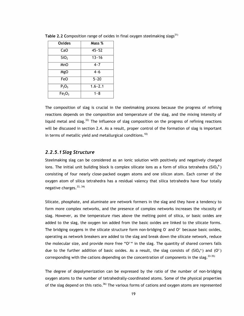
19

Table 2.2 Composition range of oxides in final oxygen steelmaking slags31)

Oxides Mass %

CaO 45~52

SiO2 13~16

MnO 4~7

MgO 4~6

FeO 5~20

P2O5 1.6~2.1

Fe2O3 1~8

The composition of slag is crucial in the steelmaking process because the progress of refining

reactions depends on the composition and temperature of the slag, and the mixing intensity of

liquid metal and slag.32) The influence of slag composition on the progress of refining reactions

will be discussed in section 2.4. As a result, proper control of the formation of slag is important

in terms of metallic yield and metallurgical conditions.10)

2.2.5.1 Slag Structure

Steelmaking slag can be considered as an ionic solution with positively and negatively charged

ions. The initial unit building block is complex silicate ions as a form of silica tetrahedra (SiO44-)

consisting of four nearly close-packed oxygen atoms and one silicon atom. Each corner of the

oxygen atom of silica tetrahedra has a residual valency that silica tetrahedra have four totally

negative charges.33, 34)

Silicate, phosphate, and aluminate are network formers in the slag and they have a tendency to

form more complex networks, and the presence of complex networks increases the viscosity of

slag. However, as the temperature rises above the melting point of silica, or basic oxides are

added to the slag, the oxygen ion added from the basic oxides are linked to the silicate forms.

The bridging oxygens in the silicate structure form non-bridging O- and O2- because basic oxides,

operating as network breakers are added to the slag and break down the silicate network, reduce

the molecular size, and provide more free “O2-“ in the slag. The quantity of shared corners falls

due to the further addition of basic oxides. As a result, the slag consists of (SiO44+) and (O2-)

corresponding with the cations depending on the concentration of components in the slag.33-35)

The degree of depolymerization can be expressed by the ratio of the number of non-bridging

oxygen atoms to the number of tetrahedrally-coordinated atoms. Some of the physical properties

of the slag depend on this ratio.36) The various forms of cations and oxygen atoms are represented

20

in Figure 2.9.36) The different structure of slag due to depolymerization after the addition of

basic oxides in silicate melt is illustrated in Figure 2.10. The oxygen and silicon atoms are

represented by white and black respectively, whereas metal ions are illustrated as shaded

circles.33, 36)

Figure 2.9 Representation of network of tetrahedra formed by Si etc. and oxygen atoms36)

Figure 2.10 Illustration of depolymerization after addition of metal oxides in silicate melt32)

2.2.5.2 Slag Basicity

Steelmaking slags are normally basic to dissolve acid impurities. In slags, the basic ion is

producing O2- from CaO, FeO and MgO whereas the acid substance is SiO2. The affinity of the

reaction between acid and base represents the relative strength of acid and base. This

phenomenon can be defined by the basicity of the slag.

The most common approach to measure slag basicity is basicity ratio or basicity index which is

the mass concentration ratio of the basic oxides to the acid oxides.37) The concentration ratio

between CaO and SiO2, known as the V ratio, can be given using:8)

21

2SiO%

CaO%=V (2.6)

Modified forms of V ratios are also employed.8) One of these correlations is:8)

32522 OAl%OP%SiO%

MgO%CaO%

++

+=B (2.7)

Another approach is Excess Base, which is the difference in concentration between the basic

oxides and acid oxides, expressed by the following equation. The concentration units can be mass

%, molar % or mole fraction.37)

∑ ∑−= sAcid OxideesBasic OxidB (2.8)

The concept of basicity in slags is explained by two main approaches:37)

i. The Lux-Flood approach is based on oxide ion activity in acid-base reactions, including

the exchange of O2- ions. Even though this approach is axio-metric it is hard to define

single ion activity due to the non-existence of a suitable reference or standard state and

not having an independent existence in slag systems.37)

ii. The Lewis approach is based on the ability of negative change donation, so that anions

such as O2- behave as bases in the Lewis state while cations behave as Lewis acids. This

basicity is expressed in terms of the state of polarization, or more simply the ‘state’ of

oxygen ions in the slag, so that this approach is much more applicable for slags.37)

The bulk and average values of the Lewis state can be quantified by optical basicity regarded in

terms of the electron donor power of the oxygen ions present. The meaning of electron donor

power of the oxygen is the average residual negative charge left on the oxygen that is less likely

to be polarised by the surrounding cations. Oxygen with high charge cations such as silicon and

phosphorus can be highly polarised, so their residual negative charge is low and so the optical

basicity would be low.37)

Duffy and Ingram37) suggested a correlation between optical basicity and Pauling

electronegativity. This correlation has been employed to several systems due to its being a

simpler method compared to spectroscopy measurements. The optical basicity values can be

calculated from Pauling electronegativity or from average electron densities for metal oxides in

steelmaking systems. The average value of optical basicity Λ, for a slag can be expressed by the

following equation.37)

...+Λ+Λ=Λ

YYXX BOBOAOAO XX (2.9)

22

where X is the equivalent cation fraction of each oxide. The standard state is determined to

define the state of polarization. In slag chemistry the optical basicity is based on CaO basicity

Λ(CaO)=1.

The main issue of these approaches is the excursive determination of slag components as acidic

or basic oxides and accommodating the intermediate oxide in the acidic or basic side.37) The

effective optical basicity of transition metal oxides varies due to the particular chemical

reactions within the slag. For instance, the optical basicity of the system is higher for a sulphur

equilibrium reaction in comparison to a phosphorus equilibrium reaction.37) Although the slag

basicity is expressed in many ways such as optical basicity, basicity ratio and Excess Base, there

is no absolute definition accepted in the literature.

2.2.6 Oxygen Injection

Oxygen injection is the main driving force for the rapid refining reactions by producing metal

droplets, distributing oxygen within the phases and mixing the bath for the top blown oxygen

steelmaking process. Oxygen impingement at high velocities creates a cavity on the surface of

the liquid and gas travels radially outwards from the impact region along the surface.

Accordingly, the liquid bath is dragged into motion and a recirculation flow occurs.38, 39)

Molloy40) described the jet-metal interaction in terms of three modes: dimpling, splashing and

penetrating, as illustrated in Figure 2.11. The dimpling mode occurs if there is a smooth surface

depression due to the low velocity and/or large lance height. As lance height is reduced and/or

the velocity of the jet is increased, the surface of the liquid becomes unstable until at a certain

point they broke up. This point is the onset of the splashing mode where the metal droplets are

torn from the side of the cavity. In the steelmaking process the splashing mode is desirable to

enhance the refining rates, except during an early blow. A further increase in the velocity of the

jet and a decrease in the lance height cause a deeper penetration. The amount of droplets

splashed is reduced and more metal droplets return back to the metal bath. This mode is referred

to as penetrating.40) These modes depend on the jet momentum and physical properties of the

liquid. The interaction of jet and liquid metal by multi-hole nozzle in a top blowing process is

illustrated in Figure 2.12.9)

As the CO gas bubbles due to the decarburization reaction build up in the gas-metal-slag

emulsion, the bubbles lead to a voluminous slag. The height of foamy slag rises inside the furnace

and can flow over the mouth into the space immediately around and below the process. This

phenomenon is called “slopping”. Slopping causes operational problems, reduces the refractory

23

lining life and lowers the yield of metal production due to an insufficient chemical reaction or

mass transfer in the process.41) Therefore, it is important to control and optimize the oxygen

delivered from the nozzle.

Figure 2.11 Flow behavior of jet40)

Figure 2.12 Fluid flow and splashing by multihole nozzle9)

The penetration area is another parameter occupying an important role in the refining reaction

kinetics. These phenomena will be discussed in the following sections. The criteria used in the

selection of nozzle design and lance dynamics which influence jet behavior are also discussed in

this section.

24

2.2.6.1 Jet Penetration

Jet penetration is characterized by the shape, diameter, and depth of the jet cavity.42) There

have been several experimental studies using air-water models38, 42-51) and argon/oxygen-steel

models.52-54) These studies were carried out to understand the various factors influencing the

depth of penetration and penetration diameter for the top blowing oxygen steelmaking process.

However, these studies were generally limited by experimental conditions such as flow

conditions, type of cold system, and nozzle applied, which can be practically studied at

laboratory scale. In these studies, nozzle diameter (d*), bath height (H), furnace diameter (Dc),

nozzle angle (α) and lance height (h) are considered as important factors affecting jet

penetration onto the liquid metal, and they are illustrated in Figure 2.13.

Figure 2.13 Factors affecting jet penetration44)

Banks and Chandrasekhara44) conducted an experimental study on gas impingement into a liquid.

They used both plane and circular air jets considering free-streamline and turbulent flow

impinging on water. They found that factors including penetration depth, diameter and

peripheral lip height have a strong relationship with jet momentum. They used a displaced

analysis technique to develop a correlation to predict the penetration depth of deep cavities by

circular jets:44)

( )

2

c

2

cld

hh

125dhg

M

+π=

ρ∗∗

(2.10)

25

where M is the jet momentum. The jet momentum depending on its high velocity and density

immediately after exiting the nozzle is calculated as follows:50)

( ) 2

e

2

g Ud4

M ∗π×ρ= (2.11)

where ρg is the density of the gas and Ue is the velocity of the gas exiting from nozzle.

Wakelin55) investigated the interaction of gas jet with liquids, including molten metals. But this

study was also limited to single layer systems. Qian et al.50) studied the impinging region using a

physical model consisting of an air jet and water bath. Kerosene and corn oil were used as the

second layer to investigate the role of the slag layer on the interface shape and bath circulation.

Qian et al.50) extended the existing model developed by Wakelin55) and developed a general

model to predict the penetration depth at various jet heights, and for a single-layer and two-

layer liquid bath systems. The correlation is given by50)

2

cc

2

2

3

lh

h1

h

h

K2hg

M

+

π=

ρ (2.12)

where K2 is 7.5. In the case of a two-layer liquid bath system, the density of the single liquid is

replaced by the densities of two different liquids. They found that the penetration depth behaves

similarly for a single and a two-layer liquid bath system at various jet momentums.

Koria and Lange54) carried out an experimental study on the interaction of the oxygen jet to the

molten steel for top blowing and combined blowing processes at 1600 °C. This is the only

experimental study reported using single and multi-nozzle jets. They suggested that the

penetration depth and diameter depend mainly on the pressure of the oxygen supply, lance

height, and the number and inclination angle of nozzle. The correlation between the penetration

depth and its factors proposed by Koria and Lange is widely employed:54)

66.0

3

la

0

a

2

t

5c

hg

1cos1

P

P27.1xP)d(x10x7854.0x469.4

h

h

ρα

−= (2.13)

The diameter of jet penetration is given by:

( )282.0

3

la

0

a

2

t

5c

hg

1sin11

P

P27.1xP)d(x10x7854.0x813.2

h

d

ρα+

−= (2.14)

These correlations were developed based on their own experimental results and previous

experimental results. It should be noted that these correlations are valid for non-coalescing jets.

The jets would coalescence when the inclination angle is less than 8.5° for a multiple nozzle

26

lance.54) Koria and Lange54) concluded that the penetration depth and diameter are influenced by

the blowing conditions and not by the presence of slag or the carbon content of liquid steel.

These findings were in agreement with those reported by Sharma and his co-workers.53)

Nordquist et al.42) reviewed the previous studies on jet penetration and its control parameters

and further modified the correlation by Quin et al.50) to predict the depth of penetration at

smaller nozzle diameters (2-3 mm). From the study of Nordquist et al.42), the penetration depth

is plotted as a function of lance height, gas flow rate, and nozzle diameter given in Figure 2.14.42)

As seen from the figure, decreasing the nozzle diameter and increasing oxygen flow rate

increases the velocity and momentum of the jet, which replaces more volume of the liquid and

creates a larger penetration depth.

Figure 2.14 The penetration depth as a function of nozzle diameter, lance height and gas flow

rate42)

The decrease in lance height increases the momentum of the jet delivered and its depth of

penetration.42, 50, 54) Because as the jet encounters a gas medium after discharging from the

nozzle, its velocity decreases in proportion to the density of the gas medium, which further

decreases its momentum.42) This topic will be further discussed in section 2.2.6.3.

2.2.6.2 Impact Area

The region formed by oxygen impingement is known as the “impact area” or “hot spot” and it is

the contact area between the oxygen and metal surface.10) Many suggestions about the geometry

of the impact area such as paraboloid, ellipsoid or Gaussian form have been made in the past.46,

27

56, 57) The impact area can be approximated as a function of the penetration depth and

diameter, which is directly related to lance dynamics, as discussed in section 2.2.6.1.

The total impact area can be found by adding the individual impact spots of every nozzle.8)

Therefore, the area can be extended by increasing the number of nozzles applied. In previous

studies by Blanco and Diaz58) and Martin et al.59), the reaction area created by a 4-nozzle lance

was assumed to be 32 m2 for a 250-300 t oxygen steelmaking process. In some studies the impact

area was assumed to be equal to the cross sectional area of the furnace. The average cross

sectional area of the bath is approximated to be 22 m2 at FG=60 m3/min for a top and bottom

blowing oxygen steelmaking process.60)

2.2.6.3 Nozzle Design

In oxygen steelmaking, oxygen is blown with approximately 8-10 atm of inlet pressure through a

convergent-divergent (Laval) nozzle which transforms high pressure energy at the nozzle inlet

into kinetic energy. The jet speed at the nozzle exit is between Mach 1.5 to 2.2.15) The velocity

of the jet is represented by the Mach number, which is a dimensionless number that relates the

speed of fluids to the speed of sound. This relationship is shown in Equation (2.15). If the speed

of a jet is more than Mach 1, the speed is called “supersonic”.

U

UM e= (2.15)

Here Ue is the velocity of the jet (m/s) and U is the velocity of sound (m/s). Oxygen is blown

through the lance tip, which is made from a high thermal conductivity cast copper alloy with

precisely machined nozzles. A typical five nozzle lance tip is illustrated in Figure 2.15. Cooling

water is crucial to preventing the lance from melting during a blow. The oxygen flow rate ranges

from 560 to 1000 Nm3/min depending on the industrial practice16, 61) and is related to n nozzles of

throat diameter d* (m) using:8)

0

0

2

5

O

T

P*)d(n10x414.1Q

2ζ= (2.16)

Where ξ is the coefficient of the flow rate, lies in the range 0.95-0.97. T0 is the temperature at

the nozzle entrance (K). Generally, the flow rate of oxygen into oxygen steelmaking is limited by

the capacity of the hood above the furnace, the gas cleaning system, and the oxygen pressure

available.16, 61)

As oxygen travels through the converging side of the nozzle it accelerates and reaches a sonic

velocity. After the diverging section the oxygen expands and the velocity becomes supersonic.16)

The flow trend of oxygen is divided into three regimes, core, supersonic, and subsonic regions.62)

28

In the core region the jet speed remains constant. At the end of the potential core the jet is

transformed into a supersonic region. As the jet travels away from the nozzle it is retarded by

the process atmosphere so that both radial and axial velocities gradually decrease until the jet

becomes fully subsonic some distance away from the nozzle.62-64) These regimes with Laval nozzle

are given in Figure 2.16.62)

Figure 2.15 The schematic diagram of convergent-divergent nozzle16)

The potential length of the core of the jet x1, varies from three to eight times the nozzle exit

diameter d1. The main factors affecting the length of the supersonic core are the blowing factors

and the ratio of densities of the gas jet and ambient medium. With top blowing the ratio would

vary throughout depending on the oxygen flow rate, the lance height, and how far the blow has

actually progressed.8)

Figure 2.16 The flow regimes in a supersonic nozzle62)

The pressure of nozzle P0, is an important design factor to be considered because the supply

pressure determines the intensity of impact onto the metal bath. Additionally, the core length of

the supersonic jet, the radial spreading and decay characteristics are influenced by the supply

pressure of the jet.65) The inlet pressure must be adjusted to provide the required velocity for

29

the prescribed mass flow rate. Otherwise, inefficient inlet pressure for a given nozzle angle

results in the jets coalescing. Thus, the dynamic pressure decreases gradually from the nozzle

exit.41) The dynamic pressure at the nozzle exit Pd,e and at any distance x, Pd,x are expressed by

the following equations.8)

2

eee,d U2

1P ρ= (2.17)

2

x,0xx,d U2

1P ρ= (2.18)

Where Uo,x is the centre line velocity at any distance x. ρe and ρx are the gas density at the nozzle

exit and at any distance x, respectively. The exit pressure of the nozzle should be equal to or

slightly higher than the ambient pressure, otherwise shock waves are generated.8) If the nozzle

exit pressure is lower than ambient there might be a dust gas absorption from the furnace into

the nozzle due to the pressure gradient at the nozzle exit.8, 63)

Multi-hole supersonic nozzles have been widely employed in top-blown oxygen steelmaking to

deliver the necessary amount of oxygen to the process. Subsequently, determining the inclination

angle α, associated with the number of nozzles is an important parameter to control the behavior

of supersonic nozzles that influence the metallurgical conditions, slopping characteristics and

lining life, and is crucial to control the coalescence behavior of the jet in the bath.66)

Coalescence occurs when the jets interfere with each other before they hit the metal bath. As a

result, their velocity decreases until it is equivalent to the velocity of the single-nozzle. 64, 66) The

number of nozzles varies from 3 to 6 holes, with an inclination angle of 10°-20° from the vertical

axis.41) The angle of the nozzle depends on the geometry of the furnace, such as the diameter of

the bath and the required impact area for the process. The relationship between the inclination

angle and number of nozzles is represented for various process capacities in Figure 2.17. The

height of the bar shows the range of inclination angle for a given multi-nozzle lance to stop the

nozzle from coalescing. 63)

Several researchers66-69) focussed on the influence of the nozzle angle on the performance of

multi-nozzle lances for top blowing steelmaking, using experimental and modelling techniques.

Based on previous studies, it is better to increase the angle of the nozzle rather than increasing

the number of nozzles because individual impact regions would be brought closer to the centre of

the bath and cause some reduction in the maximum velocity of the jet, which in turn decreases

its momentum when hitting molten metal.67, 69) Moreover, there is no advantage in increasing the

nozzle angle beyond the coalescence point because the required turbulent fluid flow would move

radially outward and be more effective on the side walls of the process.9, 29, 41) It has been

30

suggested that the optimum nozzle angle is from 12˚-12.5˚ for four-hole nozzles whereas the

angle lies between 9.5˚ to 10˚ for three-hole nozzles.67, 68)

Figure 2.17 The inclination angle is plotted as a function of number of nozzles63)

There have been numerous studies41, 63, 64, 66-73) focussing on the effects that lance dynamics has

on the flow pattern in oxygen steelmaking. Luamala et al.66) investigated the effects of blowing

parameters such as the gas flow rate, lance height, bottom blowing, nozzle angle, and number of

nozzles employed on the spitting or splashing phenomena, using the cold modelling technique.

They found that as the gas flow rate decreases from 590 to 500 Nm3/min for a given lance height

of 0.18 m, the total amount of splashing decreased by 20.6% and spitting by 44.5%. When bottom

blowing was applied, splashing and spitting decreased by 22.5% and 56.2%, respectively. The

distribution of splashes on the wall increased by 60.5% as the nozzle angle decreased from 15º to

12º. Moreover, the splashing mode is reduced significantly for a foamy slag, while introducing

bottom blowing increases splashing, particularly on the bottom parts of the furnace.

Higuchi and Tago41, 69, 70) emphasised the importance of a properly designed nozzle, such as

diameter and inclination angle for a better control of pressure distribution on the liquid metal.

They further designed a “nozzle twisted lance” to minimize spitting for the top-blown process.

They suggested that the shift of maximum pressure distribution from the lance axis reduced the

spitting rate of droplets. The maximum pressure delivered to the process is the same as with

conventional lance design for a twisted angle of 11.4˚. Zhong et al.73) also studied the splashing

effect for conventional and twisted nozzles. They suggested that a twisted nozzle with large flow

rates can be employed for splashing processes.

Sambasivam et al.72) suggested a new lance design to improve process control using

computational and experimental tools. The new lance design has six peripheral supersonic

31

nozzles and one larger sub-sonic central nozzle that will be controlled separately by the separate

supply gas given in Figure 2.18.

Regarding the new design, the oxygen flow rate can be adjusted to create a larger interfacial

area with respect to the lance.72) An optimum flow rate through the central jet can be obtained

to create a balance between improved droplet generation and control of the splashing or spitting

behavior of the jet. The sub-sonic central nozzle has a converging section to provide a wide range

of impact velocities that reduce slag foaming. The central nozzle hits the liquid metal vertically

and forms a strong shear stress on the surface. Augmentation of the interfacial area between slag

and metal phases and penetration of the oxygen jet through the metal is expected to increase

with the new lance design.72)

Figure 2.18 The illustration of seven-hole lance design with a subsonic central nozzle72)

The industrial gas supply company, Praxair, have promoted CoJet Technology based on a

coherent jet which they claim improves metal productivity.65, 74) A coherent jet is capable of

maintaining the characteristics of the jet such as exit diameter and velocity. Accordingly, the

concentration of force onto the metal bath over long distances is higher than those created by a

supersonic jet. A coherent jet consists of a convergent-divergent nozzle and a surrounding flame

envelope created by combustion of fuel and oxidant. The design of a coherent jet is, (i) the

length of its supersonic core is higher (ii) the impact pressure is higher, and (iii) the rate of

spreading and decay is lower.74) The wall mounted injection nozzle with a fixed lance has an

impact of decarburization rate with no splashing because the length of the core can be altered in

accordance with the operating conditions. In Figure 2.19, the different effect of both coherent

and supersonic jets on a metal surface, as claimed by Praxair, is shown schematically.65)

32

Figure 2.19 The different effects of coherent and supersonic jets on metal surface 65)

Praxair65, 74) investigated the effects of coherent and supersonic jets on the behavior of jets using

cold modelling. They compared the results of axial velocity for both jets for a defined flow rate

given in Figure 2.20.74) From Figure 2.19 and Figure 2.20, it can be concluded that a coherent jet

creates a deeper penetration and has a better mixing capacity in the top blowing oxygen

steelmaking process. It is claimed that the slag would have a lower concentration of FeO,

resulting in improved metal productivity and decreased splashing.65, 74)

Figure 2.20 A comparison of axial velocity of coherent and supersonic jets74)

2.2.6.4 Lance Height

Lance height is defined as the distance between the nozzle exit and surface of the metal (Figure

2.13). The oxygen blowing rate is adjusted with respect to the lance height to control the

intensity of the oxygen impinging on the liquid metal surface that affects control of the slag, gas,

and metal recirculation due to the height and nature of the slag.72) Variations in lance height are

called “soft” and “hard” blowing, respectively, for higher and lower heights.71, 72) Dynamic

variations in lance height during a blow are described below:16, 61)

33

In the early part of a blow the lance is generally placed at a higher position to promote slag

formation for refining reactions, and to stop the lance tip from making contact with the scrap.

Otherwise, the lance tip could be damaged which may cause a water leak in the process and a

possibly dangerous steam explosion. Thus, the flow pattern becomes similar to the splashing

mode.8, 63) As a result, the initial lance distance is an important parameter to be determined for a

given gas flow rate.

Koria63) developed an empirical correlation between the initial lance height hi and the bath

diameter db by using industrial data from different practices. The correlation is given below:63)

04.1

bi d541.0h = (2.19)

The correlation between bath diameter and process capacity Mt (t) was proposed using:63)

386.0

tb M704.0d = (2.20)

As the oxygen blow proceeds the lance is gradually lowered towards the bath to increase the

refining reactions and contribute to the formation of a foamy slag. Towards the end of the blow

the lance height remains constant.16)

Dynamic variation in lance height differs from one plant to another. During a blow the lance

height varies from 1.5 to 3.8 m depending on the blown pattern employed for a particular

practice. The lance height is kept higher in the initial part of the blow and decreased gradually as

the blow proceeds, as illustrated in Figure 2.21.

Figure 2.21 The lance height as a function of the process time from different plants8)

34

2.2.7 Temperature Profile of the Process

In the oxygen steelmaking process there is a wide temperature difference ranging from 1200 to

1600 °C during the blow. These temperatures are difficult to measure and are postulated to be

inconsistent because of the heterogeneous composition of slag and an impact area at higher

temperatures.10) However, it is believed from previous experimental and modelling studies75, 76)

that the temperature profile of a metal bath (Tb) increases linearly during an oxygen blow.

Chatterjee et al.15) studied various aspects of top blowing oxygen steelmaking such as bath

recirculation, rate of scrap melting, and decarburization reaction. They measured temperature

variations within the bath using a thermocouple positioned in the refractory lining below the

level of the bath. They suggested that temperature gradients vary from 10 °C to 40 °C every 5-10

s in the first half of the blow. This temperature variation was expected to be higher during a soft

blow period.15)

It is believed that the temperature of the slag is higher than the bath.8, 76) It is claimed that the

temperature differences are higher (almost 300 °C) during an early blow followed by a decrease

of 50 °C towards the end of the blow.8) Masui et al.76) also measured a 50°C temperature

difference between slag and bath during an entire blow.

The temperature at the impact area in the actual process is difficult to measure because of the

slag phase which interacts with the jet and removes heat from the impact area.8) There are few

experimental studies77-80) on measuring the temperature profile of the impact area during a blow.

Koch et al.78, 79) measured the impact temperature of a 50 kg reactor and suggested that the

impact temperature is a function of the oxygen delivered to the system. It was observed that an

increase in the oxygen flow rate accelerates the temperature of the impact area significantly.

Based on their experiments, the temperature at the impact area increases very rapidly in the

early blow and remains at a maximum level during the active decarburization period. Towards

the end of the blow the temperature at the impact area disappears. Koch et al. claimed that the

temperature at the impact area reaches 2400-2600 K during the main blow.8, 81)

Lee et al.81) proposed a correlation for the temperature of the impact area as a function of the

oxygen flow rate using the experimental study of Koch et al. for the active decarburization

period. They assumed that the temperature developed at the impact area is increased locally by

the oxidation of iron, which is controlled by the oxygen flow rate that drives the refining reaction

faster.81) This relationship is given by:81)

Ghotzone F21816)K(T += (2.21)

35

where the first value at the right hand side represents the average bath temperature during the

period between 20 to 80% of blowing time. It should be noted that the temperature profiles in

this process vary depending on the specific operating conditions.82)

2.2.8 Process Control of the Process

A number of process control systems have been developed since the early commercialization of

top blown process to optimize the process and effectively reduce the costs. Process control

systems vary from one plant to another and can be divided into two groups, static control and

dynamic control.

A static control system is based on charge control in terms of mass and heat balances to

determine the amount of oxygen to be blown and the amount of additions to be charged to the

process using the initial and final information about the process.16, 32) The time sequence of the

charge control system and material handling are shown in Figure 2.22.32) Each blowing practice

can be called “heat”. As seen in Figure 2.22, for Heat B there is a preliminary calculation to

determine the initial amount of hot metal and scrap charge required, depending on the amount

of steel aimed for and the tap temperature and carbon content of steel aimed for. Followed by a

calculation of the amount of flux, coolant, and oxygen required based on a hot metal composition

analysis conducted before the blowing period. During the initial stage of the blow for Heat B,

oxygen trim calculations are performed to determine the oxygen required utilizing the actual

amount of flux added to Heat B.16)

Figure 2.22 The time sequence of a charge control system and material handling for the oxygen

steelmaking process32)

36

Dynamic control is based on the measurement of online temperature and a determination of the

chemical analysis of the steel bath and slag without interrupting the oxygen blow.16, 17) Dynamic

control consists of a few control schemes. They are, a) a gas monitoring scheme based on a

continuous carbon balance during the process. The system determines the amount of carbon to

be oxidized by analysing dust free off-gas samples of CO and CO2,16) b) optical and laser sensors

which measure the amount of emitted light from the mouth of the furnace to estimate the

carbon level and bath temperature of the steel, respectively,16, 83) c) sub-lance technology, which

is used to measure the carbon content and temperature of the bath without interrupting the blow

before the end of the blow, and determines the additional amount of oxygen required to be

blown, or the amount of coolants to be charged,16) d) drop-in thermocouples for a quick-tap,

which is used for measuring the temperature without turning the process down, e) sonic analysis,

which is believed to provide information on the decarburization reaction and slag foaming.16) Due

to the intensity of the sound, the process can be controlled by altering the lance height or oxygen

flow rate, and f) lance height control is an important control system that determines the

behavior of the flow, and thereby the refining reactions. Variations in the lance height is

discussed in section 2.2.6.4.16)

Figure 2.23 An example of fully automatic control system32)

Iida et al.32) proposed a control system that included a device for measuring lance vibration and a

probe attached to the sub-lance to measure slag foaming using the following empirical

relationship:

37

M

O

f BhaQ

bGh

2

++−

= (2.22)

where G is the acceleration of lance vibration (cm/s2), hf is the foamy slag height (m), BM is the

furnace-bottom height correction (m), a and b are constants. An example of a fully automatic

static and dynamic control system is shown schematically in Figure 2.23.32) The process control

system is divided into 4 sub-systems. Sub-systems A and B perform the duties of static process

control and sub-systems C and D manage the dynamic control.

2.3 Thermodynamic Fundamentals

The oxygen steelmaking process is an open and heterogeneous system which allows matter and

energy to transfer between the system and its surrounding environment. Hot metal, scrap, ore,

oxygen, flux, and lance cooling water are transferred into the system and steel, slag, and exhaust

gases are transferred from the system.8) Thermodynamics provides information on the equilibrium

composition of phases under a set of conditions during the blow from thermodynamic properties

of the components in the system. During the oxygen steelmaking process, oxidation reactions

occur under non-equilibrium conditions such that predictions based on thermodynamics will be

insufficient to control the system. However, these predictions can be used to determine the

limits of the system and describe the favourable direction of the reactions occurring in the

system.

The equilibrium calculation is a strong function of Gibbs free energy. Gibbs free energy is a

function of the enthalpy and entropy of the system. Changes in enthalpy ∆H, and entropy ∆S, of

the system at temperature T, are defined by the following equations.84)

( ) ( ) ( ) ( )( )∫ ∑∑∑∑ −+∆−∆=∆ °°°T

298

pp298298T dTtstanreacCproductsCtstanreacHproductsHH (2.23)

where Cp is the heat capacity. The heat capacity data is often determined in the best-fit equation

with a limited range of temperature using:8)

2

p cTbTaC −++= (2.24)

where a, b and c are constants.

∑ ∑−=∆ tstanreacproducts SSS (2.25)

Accordingly, a variation of the standard free energy change with temperature is given by:84)

38

∫ ∫∆

−∆−∆+∆=∆ °°°T

298

T

298

p

298p298TT

dTCTSTdTCHG (2.26)

where ∆H˚ and ∆G˚ are changes in enthalpy and Gibbs free energy at a standard state,

respectively. The standard state is usually referred to as pure substance at 298.15 K and 1 atm

pressure.8) As the process proceeds at a constant temperature and pressure the Gibbs free energy

of the system decreases. The reaction is thermodynamically favoured when the Gibbs free energy

of the system is at a minimum.13, 84)

2.3.1 Thermodynamics of Liquid Iron

Liquid iron in the steelmaking process is a solution where iron is the solvent and other elements

such as carbon, manganese, and phosphorus are the solutes. The species dissolved in liquid iron

behave as a non-ideal dilute solution. The activity of elements in liquid iron can be determined

using Henry’s Law8)

( )iii %massfh = (2.27)

where hi is the Henrian activity of species i, ƒi is the Henrian activity coefficient of species i and

(mass %)i is the mass concentration of solute i in liquid iron. The relationship between the Henrian

activity coefficient and Raultian activity coefficient are expressed below8)

i

0

ii fγ=γ (2.28)

where γi˚ is the Raultian activity coefficient of species i at a standard state. In liquid iron the

solute atoms interacted with each other as a function of the composition of liquid iron and a

mass concentration of solutes during the process. The activity coefficient of elements dissolved

in liquid iron is obtained using:8)

( ) ( )∑+= i

j

ii

i

ii %masse%masseflog (2.29)

∑ε+ε= i

j

ii

i

ii xxfln (2.30)

where i

ie and j

ie are the interaction coefficient of solute i and the interaction coefficient

between solutes i and j in liquid iron, respectively. For the species in liquid iron the variation of

ln ƒi is due to the mole fraction of species whereas the variation of log ƒi is due to the mass

concentration of species. The first order interaction coefficients of major elements dissolved in

liquid iron at 1600 °C are given in Table 2.3.85) The second-order interaction coefficients are also

included in Equations (2.29) and (2.30) when log fi (or ln fi) is not a linear function of the

39

concentration of species. However, Equations (2.29) and (2.30) are only valid for oxygen

steelmaking systems.8)

Table 2.3 The first order interaction coefficients of elements dissolved in liquid iron at 1600 °C86)

i/j Si P Mn C S O

Si 0.11 0.11 0.00 0.18 0.06 -0.23 P 0.12 0.06 0.00 0.13 0.03 0.13 Mn 0.00 0.00 0.00 -0.07 -0.05 -0.08 C 0.08 0.05 -0.01 0.14 0.05 -0.34 S 0.06 0.29 -0.03 0.11 -0.03 -0.27 O -0.13 0.07 -0.02 -0.45 -0.13 -0.20

2.3.2 Thermodynamics of Steelmaking Slag

Slag is a liquid solution of molten oxides. The most important oxides of slag are MnO, SiO2, CaO,

MgO, P2O5 and FetO which represent all iron oxides in the form of FeO, Fe2O3 and Fe3O4 in the slag

phase. The activities of oxides in slag expressed in the Raultian standard state using:8)

iii xa γ= (2.31)

where ai is the Raultian activity of species i, and xi is the mole fraction of component i in slag

phase. The Raultian activity coefficient is determined as a function of the temperature and the

composition of other oxides in slag.8)

Many experimental studies87-123) on the activities of oxide component have been performed for

steelmaking slag systems. An examination of thermodynamics for oxygen steelmaking is beyond

the scope of this study, although well known studies are given as an example to represent the

activity values for the major metal oxides in slag.

Elliott99) studied the activities of CaO, FeO and SiO2 based on the Gibbs Duhem relationship in a

CaO-FeO-SiO2 system containing small quantities of MgO and low concentrations of MnO and P2O5

at 1600°C using experimental data from Taylor and Chipman90) and Winkler and Chipman.92) The

activity curves for FeO are illustrated schematically in Figure 2.24.124) The effect of MgO

concentration was considered to be similar to CaO on a molar basis and a standard state of FeO

was chosen as pure liquid FeO in equilibrium with pure iron in Figure 2.24.124) It should be noted

that the addition of lime in ferrous oxide at a constant (CaO+FeO)/SiO2 ratio increases the

activity coefficient of FeO in the slag.33)

40

The activities of SiO2 and CaO are illustrated by the plot of log γ of SiO2 and CaO in Figure 2.25 and

Figure 2.26, respectively.124) The standard states of CaO and SiO2 were chosen as pure solid CaO

in equilibrium with the melt, and pure solid SiO2.124)

Figure 2.24 The isoactivity lines of FeO in CaO-MgO-FeO-SiO2 system at 1600 °C as a function of

mass fraction after Taylor and Chipman124)

Figure 2.25 The activity coefficient of SiO2 in CaO-MgO-FeO-SiO2 system at 1600 °C as a function

of molar fraction after Taylor and Chipman34)

41

The activities of MnO in the ternary system CaO-SiO2-MnO at 1500 to 1650 °C were measured by

Abraham, Davies and Richardson.125) The activity of MnO in the system CaO-SiO2-MnO at 1650 °C is

given in Figure 2.27.126) The standard state of MnO was chosen as pure solid MnO in equilibrium

with the melt.34, 126)

Figure 2.26 The activity coefficient of CaO in CaO-MgO-FeO-SiO2 system at 1600°C as a function

of molar fraction after Taylor and Chipman34)

Figure 2.27 The activity of MnO in CaO- SiO2-MnO system at 1650°C as a function of molar

fraction after Abraham, Davies and Richardson125)

42

Richardson33) suggested that the ideal silicate mixing model can be used when two binary silicate

systems containing the same mole fraction of SiO2 were mixed. Consequently, the free energy of

the system will decrease due to the random mixing of cations such as Ca2+ and Fe2+. The activities

of FeO and MnO can be reproduced for the mole fraction of SiO2 ranging from 0.42 to 0.58 by the

ideal silicate mixing model, which agreed with experimental data from Taylor and Chipman, and

Abraham, Davies, and Richardson.127)

The activity data for metal oxides in slag have been predicted based on experimental studies.

However, these are generally limited studies with experimental conditions such as the

composition and temperature of a molten slag system, which can be practically studied at

laboratory scale for a limited range of temperature and composition. Although these studies

provide qualitative information on activity data, it is difficult to apply the findings to predict the

equilibrium composition of slag over a full range of operating conditions.

2.3.3 Thermodynamic Modelling of Oxygen Steelmaking

Thermodynamic modelling is a well established technique that provides information on the

equilibrium distribution of elements within the phases, the heat generated or consumed by these

chemical reactions, and the behavior of species in solution (as opposed to their behavior as pure

species).

Thermodynamic modelling is based on the 2nd law of Thermodynamics and the equilibrium

calculations are made using the Gibbs free energy minimization technique developed from this

law. The basis of this method is to minimize the Gibbs free energy of the system at a constant

temperature and pressure using:128)

( ) minalnRTnnGi

i

0

ii

i

ii =+µ=µ= ∑∑ (2.32)

where i represents the components of a solution and Gi represents the partial molar free energy

of i in the solution. The free energy change of the system due to mixing is the difference

between the Gibbs free energy of the system before and after mixing, as given in the following

equation.129)

∑=−=∆ ii

0

tot alnnRTGGG (2.33)

Here the variables R, T, ni refer to the gas constant, temperature, and mole of species i,

respectively. µ0 denotes the standard chemical potential and a refers to activity. Two constraints

should be satisfied, ni must be non-negative and total moles of the elements in the system must

be equal to a summation of moles in the species in each phase, as given in Eq. (2.34).

43

bjan

k

1i

jii =∑=

(2.34)

where aji is the number of g atoms of element j and bj is the total atom of element j. This is a

standard optimization problem that can be solved using the Lagrange method of unknown

multipliers. The equations that must be solved to obtain the composition of the system are not

all linear in regards to the composition variables. The Newton-Raphson method is used to solve

the equations using initial estimates of compositions nj, and Lagrangian multipliers λi, for a given

quantity of species n and temperature. This method involves a Taylor series expansion of the

appropriate equations, ignoring the second and higher orders.130, 131)

In developing thermodynamic models, the phases and the possible species within the system need

to be defined carefully. All the species defined in the system require thermochemical data such

as heat capacity, enthalpy, and entropy as functions of temperature for pure species before the

Gibbs energy minimization techniques can be applied. Fortunately, large databases of critically

evaluated thermodynamic data have been compiled by internationally recognised groups such as

NASA and NPL.

The appropriate solution models for each phase also need to be evaluated based on solution

structure and behavior. The initial quantities of species within the phases and operating

conditions are then entered. Equilibrium calculations are evaluated based on the Gibbs energy

minimization technique which is readily available in commercial thermochemical software. The

most widely used packages are Thermo-Calc, Factsage, MTData, Thermodata, HSC, Chemix and

Gemini2.128, 132) These softwares combine computational codes for databases and equilibrium

calculations to extend the applications in different metallurgical systems.132, 133) For example,

Chemix, Thermo-Calc and MTData offer flexibility to choose a solution model such as polynomial,

Redlich-Kister and Margules depending on the user’s system. HSC has a limitation on the solution

behavior selection. The activity coefficients can only be entered as a constant number or a

polynomial function of composition and temperature. Nevertheless, HSC has been widely used in

industry because of its simplicity.128)

One of the major challenges in a thermodynamic model of steelmaking is a determination of an

appropriate solution model for each phase in the steelmaking process. Models of solution

behavior allow experimental results for particular systems to be generalised and make

predictions of solution behavior away from the conditions of the original empirical data set.

However, interactions between different species in a phase at different concentrations and

temperatures are complex, particularly where basic molecular forms in a phase vary with

44

concentration and temperature, in these instances it is hard to find a solution model that works

well for all conditions.

In the case of liquid iron, a dilute solution model using empirically determined “interaction”

parameters is well established and can be readily applied to these problems. The dilute solution

model is based on Henry’s Law which assumes that the activity of solute has a linear relationship

with concentration.134) However, for slag the solution behavior of the phase is challenging to

model because it is difficult to describe the complex molecular structure of slag itself, which

makes an interpretation of the experimental data troublesome. Moreover, a lack of knowledge of

the interaction between different metal oxides in slag creates further difficulties in developing

robust thermodynamic models of slags.133) However, the importance of molten oxide solution

behavior to materials science, geology, and inorganic chemistry has meant that a large body of

work exists around this work.32, 126) Several models of multi-component oxide systems have been

developed, these include ionic two sub-lattice, regular solution, cell, associated solution, and

modified quasi-chemical models.135-143) Although the regular solution model is simple to employ,

cell and modified quasi-chemical models are more appropriate for studying steelmaking slags.133)

Kapoor and Frohberg139) suggested the cell model where oxides are described by two sub-lattices.

Gaye and Wellfringer140) modified this model to include poly-anionic and multi-component melts.

An anionic vacancy free sub-lattice occupied by oxygen ions and a cationic sub-lattice occupied

by cations and cationic entities exists according to the order of their decreasing electrical

charge.133) Cationic entity is defined as cations doubly bonded to one oxygen. This extension is

helpful to describe the behavior of some oxides which do not release all their oxygen to anionic

sub-lattice, such as P2O5.135) A change in the state of oxygen ions polarization can be given:

−− =+ O2OO 20 (2.35)

The state of polarization of oxygen ions is affected by the surrounding cations. Therefore, slag is

a mixture of cells where the oxygen atom is centred and two cations are surrounded by oxygen

which are asymmetric (MiOMj) and symmetric (MiOMi) cells.84, 139) There are two types of energy

parameters required to describe the formation of cells to determine the activity coefficients of

metal oxides in slag as a function of composition and temperature, (i) the formation energy Wij,

of the asymmetric cells corresponding to the reaction between two symmetric cells MiOMi and

MjOMj : (ii) interaction energies limited to one parameter per couple of cations and binary

interaction energy Eij describing the binary interaction energy between symmetric and

asymmetric cells. The limitation of the cell model is that there are limited binary parameters

available for multi-component slag systems. Furthermore, the parameters are independent of

temperature.60, 144)

45

The second challenge is to determine an appropriate database with regard to the software

program. The literature is established based on experimental data for particular ranges of

temperature, pressure, and composition. An interpolation technique is applied if there is no

study available for a particular temperature, composition, and pressure. As a result, models can

give unrealistic results when studying a particular system in conditions far removed from the

experimental results that feed into the various equations described above. Whilst the modelling

of molten oxides solution behavior is complex and reliance on empirical measurements is

unsatisfactory, computational chemical thermodynamic modelling is regarded as a great success,

resulting in many useful and important predictions over many fields, including steelmaking.145)

For example, thermodynamic modelling has been successfully applied to a prediction of the

distribution of sulphur in steelmaking reactions146) using the techniques described above.

2.4 Kinetic Fundamentals

Whilst computational thermodynamics can predict the equilibrium composition of steelmaking

reactions, this technique cannot predict how fast these reactions take place and what controls

their rate. As a field of knowledge, “reaction kinetics” attempts to answer such questions.

Reaction kinetics provides information on the conditions that govern the rate at which a reaction

will occur and can describe the mechanism by which it proceeds. However, it is important to

integrate knowledge from thermodynamic equilibrium to kinetics and relate these essentially

fundamental phenomena to understand the steelmaking process more thoroughly.147)

To start with, it is important to analyze the system itself and determine its surrounds. Oxygen

steelmaking involves simultaneous multi-phase (solid-gas-liquid) interactions, chemical reactions,

heat and mass transfer, and complex flow patterns due to an interaction between the liquid

metal bath and high speed oxygen jet at high temperatures. A schematic representation of the

system is given in Figure 2.28.

The oxygen jet contacts the metal bath directly and is picked up by the molten iron. The

dissolved oxygen reacts with other elements dissolved in the molten metal at the interfaces

between metal and gas, and between metal and slag. Meanwhile, metal droplets are ejected

through the slag phase and metal droplets are simultaneously in contact with FeO in the slag. Gas

bubbles are generated due to a decarburization of metal droplets via FeO reduction. Slag-metal-

gas emulsion is formed due to refining reactions, as seen in Figure 2.28. Table 2.4 lists the major

reactions occurring within the different phases. All these refining reactions take place

simultaneously in various reaction regions that makes the process complex to analyze thoroughly.

46

Figure 2.28 The schematic representation of oxygen steelmaking regions

Table 2.4 The major reactions in an oxygen steelmaking system14)

Oxygen pick up by the metal:

O2(g) = [O] (2.36)

CO2(g) = CO(g) + [O] (2.37)

(FeO) = Fe + [O] (2.38)

(Fe2O3) = 2(FeO) + [O] (2.39)

Oxidation of elements in the metal:

[C] + [O] = CO(g) (2.40)

Fe + [O] = (FeO) (2.41)

[Si] + [O] = (SiO2) (2.42)

[Mn] + [O] = (MnO) (2.43)

2[P] + 5[O] = (P2O5) (2.44)

Oxidation of compounds in the slag:

2(FeO) + ½O2(g) = (Fe2O3) (2.45)

2(FeO) + CO2(g) = (Fe2O3) + CO(g) (2.46)

Flux reactions:

MgO(s) = (MgO) (2.47)

CaO(s) = (CaO) (2.48)

Gas reactions:

CO(g) + ½O2(g) = CO2(g) (2.49)

where [] indicates the element dissolved in iron and () indicates the compound dissolved in slag.

In general, the reaction kinetics of an element from the metal phase to the slag phase take place

in the following sequence:148)

• The mass transfer of elements from the metal phase to the slag-metal interface

47

• The mass transfer of oxygen from the gas phase to the metal-gas interface, or oxygen

dissolved from the metal phase to the slag-metal interface

• A chemical reaction of the elements at the slag-metal interface

• The mass transfer of product element from the slag-metal interface to the slag phase

In steelmaking, the chemical reactions are usually not a rate limiting step because the high

temperature of steelmaking reactions favours high reaction rates. Thus, reaction kinetics is more

likely to be controlled by the transport of elements from/to the phase interphase. Generally

speaking, the reaction rates in steelmaking operations are predicted using Fick’s 1st Law which

states that the rate of diffusion is proportional to the concentration gradient.60, 149)

( )∗−= CCV

Ak

dt

dCb (2.50)

Here variables k, A and V are the mass transfer constant and the area and volume, respectively.

Cb and C* refer to the bulk and equilibrium concentrations in mass %, respectively. It should be

noted that there are different mechanisms that control the kinetics of oxygen steelmaking.

Robertson et al.150) developed a general kinetic model for multi-component slag-metal and slag-

metal-gas reactions by assuming that the reaction rates are controlled by multi-component

transport processes in the metal, slag, and gas phases. The equilibrium and interface

concentrations of each component are calculated simultaneously and can be fed into the mass

transfer equations. This model was applied to the desulphurization reaction in liquid iron as an

example. There were some differences between the model predictions and experimental results.

Some of the important weaknesses of this model are that the ratio of the metal phase mass

transfer coefficient to the slag phase mass transfer coefficient kept constant, and changes in the

physical properties of slag such as viscosity and interfacial tension were not included in the

calculations. They suggested that this may be the reason for differences in the model predictions.

Conversely, Brooks et al.151) disagreed with using 1st order differential equations for steelmaking

systems because a reduction of Fick 1st Law to a simple 1st order differential of Equation (2.50)

involves many gross simplifications. They stated that a 1st order differential equation can be

employed when there is a small variation in the mass transfer conditions, the equilibrium drive,

and the interfacial area, which is not the case in steelmaking operations. Accordingly, they

suggested that the overall kinetics for a particular reaction in such a system can be calculated by

a simultaneous summation of the flux of a particular species at distinct interfaces in the system

represented by the equation:151)

48

∑=

=

=mi

1i

ioverall JJ (2.51)

where m is the number of distinct interfaces in the system. Brooks et al.151) showed different

approaches to deal with transient kinetic behavior in slag-metal reactions such as the bloating

phenomena of metal droplets, desulphurization in the steel ladle, and spontaneous

emulsification. For example, the model to predict the residence time of bloated and dense

droplets has been successfully applied to the experimental data152) and details of this model have

been explained elsewhere5) and will be the subject of section 2.4.1.5.

In addition to mass transfer, Belton and his co-workers153-157) pointed out that chemical reactions

at surface of the liquid play an important role in understanding the overall kinetics of multi-

phase reactions, particularly metal-gas reactions. The basis of this statement is that the

interfacial area would be limited by the surface coverage of elements such as sulphur and oxygen

present in the gas or metal phase. Accordingly, the reaction rate becomes slow. One example of

this is the control of nitrogen in liquid steel. Pehlke and Elliott158) studied the kinetics of nitrogen

dissolution in liquid iron and established that the adsorption or desorption of nitrogen is a rate

limiting step, and the presence of sulphur decreases the reaction rate significantly. Several

researchers159, 160) also obtained a similar result. Sain and Belton154) studied the kinetics of the

decarburization reaction of liquid iron via CO2 under high gas flow rates between 1160 and

1600°C. Their experiments showed that sulphur has a retarding effect on the reaction rate and

the rate of dissociative adsorption of CO2 is a rate limiting step. This result was also confirmed by

Mannion and Fruehan.161) Decarburization via CO2 is a subject of this study and will be further

discussed in section 2.4.1.1. In conclusion, chemical reactions become of interest in some

instances of oxygen steelmaking reactions.

The kinetics and mechanism of decarburization reactions, scrap melting and flux dissolution will

be discussed in the following sections, while other refining reaction kinetics will only be

mentioned briefly because it is beyond the scope of this study.

2.4.1 Kinetics of Decarburization Reactions

The progress of carbon removal is crucial in oxygen steelmaking because the oxygen blowing

period is determined with regard to the carbon content and temperature of the steel within

certain limits, prior to further processing. The products of carbon removal reactions such as CO

and CO2 provide an additional power for bath circulation and create new surfaces at the impact

zone continuously. This behavior of fluid flow enhances the kinetics of refining reactions.162) The

decarburization reaction itself is an important issue in designing the process of steelmaking.

49

Although numerous attempts have been made to describe the kinetics and mechanism of

decarburization, there still remains a gap in understanding how laboratory results can relate to

plant measurements.

It is believed that the overall decarburization reaction can be divided into three main regimes.8,

163) In the initial period of blow (regime 1), almost all the oxygen is used for silicon oxidation.8, 164)

The decarburization rate is low, but it increases linearly. During the main blow (regime 2), the

silicon content of metal is very low and nearly all the oxygen is consumed by decarburization.

Consequently, the overall decarburization rate increases with an increasing oxygen flow rate, as

shown in Figure 2.29.8, 78, 82, 163, 164)

Figure 2.29 The evolution of decarburization rates with the oxygen flow rate8)

Towards the end of a blow, the overall decarburization rate decreases linearly as the carbon

content reaches a critical limit. The critical carbon content is crucial for controlling the end

point content of carbon. Goldstein and Fruehan82) developed a relationship to predict the critical

carbon content, which suggests that the decarburization rate controlled by the oxygen flow rate

equals the decarburization rate controlled by carbon diffusion in liquid metal.

In regime 3 it has been argued that the decarburization rate becomes slower and is controlled by

carbon diffusion to the metal-slag interface due to a low level of carbon content.8, 163, 165) Based

on the bulk carbon content of metal measurement, a decarburization rate for a 200 t top blown

oxygen steelmaking process was predicted by Cicutti et al.166) The change in the carbon content

of the metal and predicted decarburization rate for different regimes with respect to time, is

given in Figure 2.30.

50

Figure 2.30 The decarburization rate is plotted as a function of time167)

It has been established that decarburization occurs in different reaction zones using various

reaction mechanisms. There are two main reaction zones considered in the literature, the bath

and emulsion zone. However, there is no agreement on the proportion of carbon refining taking

place, and in which reaction zone. Several researchers168, 169) claimed that the predominant

reaction is via the gas-metal interaction at the impact zone. Okano et al.168) studied the

decarburization reaction at three reaction zones, experimentally and theoretically. They argued

that 75-80% of carbon is removed at the impact zone and only 20% of carbon is removed in

emulsion during the main blowing time. The remaining part of the blow takes place via

nucleation of CO gas bubbles from the bath. Price170) also suggested that 65% of decarburization

occurs at the impact zone.

Conversely, a number of researchers171-174) believe that most of the decarburization reaction

takes place in the emulsion phase. Kozakevitch et al.171) observed the presence of metal droplets

in emulsion. Meyer et al.172) further quantified the amount of metal droplets generated in the

emulsion using the splashing sampling technique in a 230 t oxygen steelmaking furnace. After

these findings, researches mainly focused on understanding the kinetics of decarburization in the

emulsion phase. Chatterjee et al.15) investigated the effects of changes in process conditions on

the droplet formation and decarburization rate. Thus, the mechanism and kinetics of the reaction

is another important issue in the oxygen steelmaking process to be reviewed.

2.4.1.1 Decarburization in the Impact Zone

Reactions between the metal bath and oxidizing gasses are of particular interest because a

significant proportion of carbon removal in oxygen steelmaking occurs in the impact zone in the

reactor.161, 175, 176)

51

It is known that as oxygen from a top blown lance reaches the surface of the liquid bath it reacts

with carbon dissolved in the metal at the impact zone and forms a mixture of CO and CO2 gases.

Subsequently, dissolved carbon also reacts simultaneously with CO2 at this region. The following

equations can be used to represent decarburization reactions at the impact area:148)

[ ] )g()g(2 CO2COC =+ (2.52)

[ ] )g()g(2 COO2/1C =+ (2.53)

Decarburization reactions via gasses have been studied using two different experimental

techniques. The first method is the crucible technique where liquid iron is exposed to the

oxidizing gases to investigate the mechanism and reaction rate of decarburization. Another

method is the levitation technique where liquid iron droplets containing carbon content are

levitated in or allowed to accelerate through an oxidizing environment. The second method was

initially applied to understand the reaction kinetics in continuous steelmaking developed by the

British Iron and Steel Research Association. This process is also known as spray steelmaking.177)

This process involves the atomization of a stream of liquid metal by high speed oxygen jets. This

process creates a great interfacial area that allows for fast refining rates of impurities.177)

The possible reaction mechanisms for the above reactions are given below:

(i) A mass transfer of oxygen in the gas phase

(ii) the adsorption of oxygen into the liquid iron

(iii) a mass transfer of carbon monoxide in the gas phase

(iv) a mass transfer of carbon dioxide in the gas phase

(v) a mass transfer of carbon through the metal phase

(vi) a chemical reaction between carbon and oxygen at the interface

steps (i), (iii), and (vi) apply to the decarburization reaction with O2 whereas (iii), (iv), and (vi)

apply to the decarburization reaction with CO2. It has been postulated that the mass transfer of

carbon can be neglected at high concentrations of carbon (above critical carbon content).8, 154, 159,

161, 178-180) The adsorption of oxygen can also be neglected because oxygen has already been

present in the liquid iron.

There have been numerous studies in the literature 154, 155, 159, 161, 176, 178-203) on the mechanism and

kinetics of the decarburization of Fe-C melts with oxidizing gasses using levitation and crucible

techniques. The conclusion from previous studies is a general agreement that gaseous diffusion

controls the decarburization rate down to the critical level of carbon, where carbon diffusion in

the liquid phase becomes the rate-limiting step. However, some investigators have suggested

52

that sulphur has a determining effect on the reaction rate and chemical reaction at the

interface, and also controls the reaction rate.

In the case of the decarburization reaction via CO-CO2, Nomura and Mori186, 187) studied the

kinetics of decarburization experimentally by blowing CO-CO2 gas mixtures onto the inductively-

stirred iron-carbon melts at high and low carbon concentrations using the crucible technique.

They developed models that involve both mass transfer and chemical reactions at the melt

surface. They suggested that the decarburization reaction is limited by gas diffusion at high

carbon concentrations whereas the reaction involves a mixed control mechanism involving

gaseous diffusion, chemical reaction, and carbon diffusion at low carbon concentrations.187)

Nomura and Mori186) and Fruehan and Martonik189) claimed that the effect of sulphur (sulphur

concentration is below 0.3 mass %) is relatively small on the reaction rate in CO-CO2 gas mixture

at high carbon concentrations. Goto et al.203) also measured the change in concentration of CO2 in

carbon containing iron melts at 1600°C. These measured values were close to those calculated

based on the gas diffusion approach. They concluded that sulphur has no significant effect on the

reaction kinetics. Sain and Belton154) and Mannion and Fruehan161) studied the kinetics of

decarburization reaction in liquid iron by CO2 under high gas flow rates to reduce the effects of

mass transfer. They argued that CO2 dissociation on the surface controls the reaction rate. Lee

and Rao178, 179) investigated the effects of surface active elements, gas flow rate, partial pressure

of oxygen and gas composition. They proposed that all the parameters have an influence on the

decarburization rate. However, the rate of decarburization is markedly controlled by the

composition of gas because it determines the amount of oxygen transferred to the system. Based

on their observations, they developed a kinetic model including a mixed control of the

dissociative absorption of CO2 and gas phase mass transfer at high carbon concentration, and in

the presence of sulphur.

The studies159, 180, 182, 183, 185, 188, 190) on decarburization reaction kinetics via oxygen agree that

oxygen diffusion in the gas phase limits the system at high carbon concentrations. Ghosh and

Sen204) and Kondratev et al.198) claimed that the chemical reaction between carbon and oxygen is

the rate limiting step. However, these studies were industrial scale studies that did not include a

precise formulation of the reaction mechanism. Rao and Lee159) investigated the kinetics of

levitated molten iron-carbon specimens reacting with quaternary Ar-He-N2-O2 gas mixtures at

1700 °C at various oxygen partial pressures. They suggested that surface active elements such as

oxygen and sulphur have no effect on the kinetics of the decarburization reaction.

The current knowledge on the kinetics of the decarburization reaction via gaseous products can

be summarized as follows:

53

- At high carbon concentrations the decarburization rate is independent of carbon concentration.

However, the rate decreases with a decrease in the carbon content below the critical carbon

content.154, 155, 159, 178, 179, 189)

- Sulphur has a retarding effect on the decarburization rate via CO2. Lee and Rao178) observed that

the rate decreased significantly with an increase in sulphur concentration up to an 0.05 mass %.

Above this level the rate remains constant as a function of the sulphur concentration at 1700°C.

- The composition of gas mixture is another important factor on the rate of decarburization.178,

186) An increase in the partial pressure of CO2 increases the rate of decarburization.186) The partial

pressure of oxygen has a crucial effect on the decarburization reaction.159)

- An increase in the gas flow rate increases the rate of the reaction.176, 178, 183, 185, 189, 193, 198) In the

case of gas mixture blowing, the increased oxygen content of the gas mixture increases the rate

of decarburization.178, 198)

- An increase in the temperature of the melt has an effect on the decarburization kinetics.176, 178,

193)

Most of the experimental studies focused on the decarburization reaction of Fe-C melts or

droplets and the effect of sulphur on the reaction mechanism was investigated. There are a few

studies181, 192, 193, 196) that consider the influence of other refining reactions on decarburization

kinetics. Robertson and Jenkins181) observed the behavior of levitated droplets containing C, Si

and Al with oxygen. They found that the silicate layers formed initially on Fe-C-Si droplets which

retard the decarburization reaction. A similar behavior was observed by Sun and Pehlke.193) They

studied the kinetics of a simultaneous oxidation of carbon, silicon, manganese and sulphur in a

liquid metal droplet by oxygen and/or carbon dioxide in nitrogen gas at 1873 to 1993 K. They

observed there was a delay in silicon and manganese oxidation reactions at high temperatures

and high carbon contents because the decarburization reaction consumed most of the oxygen

supplied to the system. In the case of a low carbon content (0.4 mass %), a simultaneous

oxidation of manganese and silicon was observed in their experiments.

Blanco and Diaz58) developed a kinetic model which assumed that the removal of carbon occurs

via direct oxidation at the impact zone. They estimated the mass transfer constants by fitting

data taken from an oxygen steelmaking process. They studied different scenarios for the reaction

mechanism and suggested that the mixed control of a carbon-oxygen reaction at the gas-metal

interface and gas diffusion should be considered as a rate controlling step. However, it should be

noted that the effects of blowing conditions were not included in this study.

54

2.4.1.2 Decarburization in the Slag-Metal-Gas Emulsion

The decarburization reaction in the emulsion phase takes place via FeO reduction. On the basis of

x-ray transmission photographs4, 173, 205, 206) and an analysis of the experimental results, 4, 206, 207) it

is believed that the reaction takes place in two steps via a bubble formation. As metal droplets

are ejected from the liquid metal they react with FeO in the slag. FeO diffuses to the slag-gas

interface towards a bubble sitting on the metal-gas interface to supply oxygen. CO reduces FeO

at the slag-gas interface which is followed by a reaction at the metal-gas interface with CO2

diffusion through a gas halo.206) CO2 provides oxygen to react with carbon in the melt. These

reactions involve the sequence206)

( ) )g(2)g( COFeFeOCO +=+ (slag surface) (2.54)

[ ] )g()g(2 CO2CCO =+ (metal surface) (2.55)

The overall reaction is

( ) [ ] )g(COFeCFeO +=+ (2.56)

These sequential reactions continue until the bubble leaves the slag-metal interface.

Accordingly, the carbon content of metal droplets will decrease and numerous CO gas bubbles

will be formed. The reaction product, CO gas, provides stirring to the emulsion phase. It is

believed that the decarburization reaction via FeO reduction is responsible for the majority of

decarburization in oxygen steelmaking, and this reaction is also important to slag foaming and

slopping during the process.

The transport of oxygen through the slag phase or through bubbles surrounding the metal droplet,

transfer of carbon in the metal, interface chemical reaction, nucleation and removal of CO gas

bubbles from the reaction site may all be important in determining the rate of decarburization

reaction. Numerous researchers4, 165, 169, 173, 192, 200, 206-237) have studied the kinetics of the overall

reaction as well as the reaction steps extensively. The carbon refining reaction via FeO reduction

is summarised based on current knowledge in the following.

There is evidence that a CO gas halo formation surrounds a liquid metal droplet when the metal

droplets containing high carbon content (up to 4 mass %) reacts with an oxygen steelmaking slag.

Mulholland et al.173) first observed the gas halo surrounding Fe-C-S droplets in slag using an x-ray

fluoroscopy technique. Other researchers4, 169, 206, 236, 238, 239) provided further evidence of the

formation of a gas halo. This phenomenon may occur due to the high rate of external nucleation

of CO gas compared to internal nucleation. In such a case the energy barrier for nucleation is

reduced due to a sufficient amount of C and O available at the slag-metal interface, which is

55

called external nucleation.169) When oxygen diffuses through a droplet, CO pressure increases

with time, and if the CO pressure exceeds the ambient pressure, the metal droplet becomes

supersaturated and the reaction of oxygen and carbon becomes possible.235) Gaye and Riboud165)

further studied the observations of Mulholland et al.173) to measure the oxidation reactions

between droplets of Fe-C, Fe-C-S, and Fe-C-P in oxidizing slags at 1500˚C. It was evident that

there is a spontaneous emulsification and agitation created by CO bubbles that significantly

increases the reaction kinetics. They stated that all oxidation reactions take place simultaneously

rather than sequentially. They found that the interfacial reactions, mass transfer in gas and

metal phases are crucial steps, however, they did not suggest any control step for the

decarburization reaction. A similar conclusion was reached by Gare and Hazeldan.169) They also

carried out an experimental study to quantify the factors affecting the decarburization reaction

between liquid iron droplets and oxidizing slags. They described the decarburization reaction in

five different periods based on their x-ray observations and postulated various reaction

mechanisms for each period.

2.4.1.3 “Bloated Droplet Theory”

When the internal pressure of CO exceeds the surface energy of the metal droplet, CO gas forms

inside the metal droplet.230) The pressure of CO gas depends on the concentration of carbon and

oxygen, and the temperature and concentration of other impurities inside the metal droplet. The

build up rate of bulk oxygen depends on the difference between the oxygen absorption rate and

rate of consumption of this oxygen at the surface due to decarburization and formation of iron

oxide. 230)

As internal nucleation started, the metal droplet becomes “bloated” and the surface area

increases, therefore the reaction kinetics increases because turbulence caused by the generation

of CO bubbles inside the metal droplet promotes diffusivities.233) This bloating of metal droplets

is suggested due to an internal generation of CO bubbles. 235-237) It is worth mentioning that in the

literature some researchers use the term “swelling” instead of “bloating.”235, 237)

Baker et al.210, 212, 213) first observed a metal droplet exploding from internal CO nucleation when

passing through a mixture of oxygen and helium gas. This phenomenon was called “boiling”.

Similar observations have been done by Sun and his co-workers.200) They investigated the

decarburization and oxygen absorption rates at 1723-1843 K and found that the supply rate of

oxygen from bulk gas was faster than the oxygen consumption rate at the surface by the reaction.

It was stated that this may be due to an insufficient transfer of carbon through the interface.

They also found that the decarburization rate decreases with sulphur in the metal droplet. They

56

concluded that these steps were all crucial and developed a kinetic model that included the gas

phase and metal phase mass transfer, and interfacial reaction.

Later, Sun and his co-workers233, 235) studied the bloating behavior of metal droplets in oxidizing

slags. They carried out an experimental study to investigate the effects of the composition of the

metal droplet on the reaction rate of decarburization in oxidizing slag. They developed a kinetic

model incorporating the liquid phase mass transfer of substitutes such as carbon, silicon,

manganese, the gas phase mass transfer and the interfacial reaction controls. They found that

the decarburization rate was retarded due to other oxidation reactions in the metal droplets. The

kinetic model results for the decarburization rate agreed with those of their experimental

observations and Molloseau and Fruehan’s experimental study at low FeO content (<5 mass %).

However, the decarburization rate predicted by Sun et al.235) was underestimated when the FeO

content was higher than 10%. They stated that the disagreement might be due to the bloating

behavior of droplets because they did not include an increase in the interfacial area and the

contribution of reactions inside the metal droplets. They found that there is an incubation period

for the bloating phenomena and suggested that some time is required to build up the over-

saturation level of CO nucleation within the droplet. Accordingly, they concluded that CO

nucleation within the droplet is responsible for the droplets bloating.

A similar conclusion was also drawn by Fruehan and his colleagues.4, 206) Firstly, Min and

Fruehan206) carried out an experimental study to measure the decarburization rate of droplets in

steelmaking slags containing low FeO content. They proposed a rate controlling step of

decarburization based on the sulphur concentration of metal droplets. At high sulphur

concentrations (>0.01 mass %), the dissociation of CO2 on the surface of a metal drop limits the

reaction whereas it is controlled by the mass transfer in the slag, the mass transfer in the gas

halo, and a chemical reaction at the metal-gas surface. Their observations indicated that the

carbon content of droplets also has an influence on the reaction rate. However, in their study

they couldn’t explain the relationship between the carbon content and decarburization rate.

Molloseau and Fruehan4) further studied this phenomenon for slags containing between 3 and 35

mass % FeO. This study is the first to investigate the behavior of dense and bloated droplets

under various FeO concentrations. They measured that the reaction rate of bloated droplets was

one to two orders of magnitude faster than the rates of dense droplets. Based on their

observations they suggested that FeO transfer in the slag is a possible rate limiting step for the

decarburization rate of bloated droplets whereas the reaction rate of dense droplets is controlled

by dissociation of CO2 on the metal.

57

Chen and Coley236, 237) conducted an experimental study to predict the nucleation rate of CO

inside the metal droplets using an x-ray fluoroscopy technique at various temperatures. They

compared the swelling rate with the total volume of gas evolved during the reactions. They

investigated the effects of droplet size on the gas generation rate and found that the diameter of

the droplets increased to 1.5 times their original size. This observation agreed with those

reported by Molloseau and Fruehan.4) It was found that the reaction rate increases as the size of

the droplet increases. The gas generation rate was suggested to be controlled by the rate of

nucleation of CO gas bubbles inside the droplet due to a dependency of the reaction rate on the

droplet size. They reported that the critical supersaturation pressure of the nucleation was two

orders of magnitude less than that predicted by nucleation theory.

The current observations showed that metal droplets are “bloated” with CO gas, generated

during the active decarburization period when FeO concentration in the slag is higher than 10

mass % in the emulsion phase. The droplets become less dense and are suspended for a longer

time in the emulsion. Alternatively, if the rate of carbon removal is weak, CO gas as a reaction

product escapes easily and is detached from the droplet. As a result, the metal droplet maintains

its original shape.240) These studies indicated that droplet emulsification was a crucial factor in

the decarburization kinetics of oxygen steelmaking. Some industrial observations171, 172) provided

supportive evidence for these findings.

In summary, there is no agreement on the mechanism, controlling step, and reaction rate of the

decarburization reaction in the emulsion phase. There is firm evidence that the decarburization

rate increases with an increase in the temperature of the slag, the FeO content in the slag, the

carbon content in the metal droplet and droplet size, however, the rate decreases with an

increase in sulphur and silicon content in the metal droplet, and the ambient pressure.4, 165, 200, 206,

235)

Whatever the mechanism is, refining rates in the emulsion phase can be increased dramatically

by the interfacial area between the metal droplets and the slag. Meyer et al.172) claimed that the

surface area for carbon-oxygen reaction reaches 18580 m2/t during oxygen steelmaking. Brooks

and Subagyo241) reported a relationship to predict the total interfacial area as a function of drop

size and fraction of metal emulsified based on the assumption of an ideal system with mono-sized

liquid spheres of liquid metal suspended in the slag, given as follows:241)

pD

87.0

tonne

Area ϕ= (2.57)

58

where φ is the fraction of metal in the emulsion to the total metal in the furnace and Dp is the

diameter of mono-sized droplets (m). Based on this relationship, if 50% of the total metal is in

the emulsion and the size of the droplets is 1 mm, the total surface area would be 436 m2/t.241)

Since decarburization kinetics in the emulsion are induced by the interfacial area, the reaction

rate depends on (i) the number of metal droplets generated (ii) the droplet size distribution and

(iii) the residence time of the metal droplets.242) The residence time represents the required time

to react with the slag, whereas the quantity of droplets and droplet size distribution provide

information on the size of the interfacial area. As a result the current knowledge on droplet

generation, droplet residence time, and droplet size distribution should be reviewed to better

understand the kinetics of refining reactions. It will be discussed in the following section.

2.4.1.4 Generation of Metal Droplets

Several studies have been carried out in recent years to develop a better understanding of the

mechanism of the kinetics of oxygen steelmaking. 5, 38, 39, 71, 147, 150, 152, 166, 206, 235, 242-249) As an

outcome of these studies, it has been established that droplet generation is a crucial part of the

process kinetics of oxygen steelmaking because it contributes to a large interfacial area during

the blow which in turn affects mass transfer between the metal and the slag.

In top blowing practice, as the oxygen jet impinges into the liquid bath, the jet spreads out the

slag phase, interacts with liquid metal and creates a cavity at the interface between the slag and

the metal phases. Metal droplets are torn from the cavity and ejected out of the metal bath into

the slag-metal-gas emulsion due to the high speed jet throughout the blow.38) This phenomenon

of droplet generation by an impingement of oxygen on the metal surface is governed by the laws

of mechanics, which are based on the force balance on the metal surface.249)

There are three main forces influencing droplet generation, inertial, gravitational, and surface

forces. Gravitational and surface tension forces tend to stabilize the interface, whilst the inertial

force tends to destabilize the interface. The impingement of a gas jet causes a depression on the

surface of the metal bath. As jet momentum is low, the metal phase has a tendency to self-

adjust by changing the shape of the depression to keep the force balance on the droplet. Under

dynamic blowing conditions, inertial forces dominate other forces. Therefore, the inter-facial

flow increases the frequency of surface waves until, at a certain point, surface waves break up

and metal droplets are torn off, which leads to an increased inter-facial area.38, 249, 250)

59

Figure 2.31 The effect of jet momentum on drop generation rate249)

Regarding the balance of forces exerted on the metal surface, Standish and He249) reported that

two different mechanisms of droplet generation exist due to a variation in the gas flow rate, as

shown in Figure 2.31. As seen in Figure 2.31, when the oxygen flow rate is low, a weak depression

occurs on the metal surface that corresponds to the line AB. A single droplet is generated and

ejected at the edge of the small wave. This region is called “dropping” and is represented in

Figure 2.32(a).

(a) (b)

Figure 2.32 Two regions of droplet generation249)

An increase in the oxygen flow rate results in the growth of waves in the impact area. As a result,

there is an increment in the quantity of droplets and also large tears of liquid are produced at

the edge of the impact area. Each of the waves might cause an ejection of liquid tears at the

edge of the impact area. From experiments undertaken by Standish and He,249) it has been found

that the formation of a tear of liquid starts with a wave which expands gradually as it moves up

along the surface of the impact area. The liquid tear is impacted by the deflected gas flow to

become several small drops. Meanwhile, a number of individual drops are directly generated at

60

the impact area of the jet. This region is called “swarming,” is shown in Figure 2.32(b) and

corresponds to the line BD in Figure 2.31.249) The dropping and swarming regions affect the

increment level of droplet generation rate differently. It has been observed that the droplet

generation rate in the swarming region is higher than the dropping region due to a larger

penetration depth on the furnace.248)

There have been two important factors affecting droplet generation.39) They are the momentum

intensity of the gas jet and the physical properties of liquid metal. The momentum intensity of

the gas jet is an external factor defined as the ratio between jet momentum a certain distance

from the nozzle exit and the corresponding jet cross sectional area. The momentum intensity can

be increased by either decreasing lance height or increasing the oxygen flow rate.39)

Figure 2.33 shows the predicted droplet generation rate with respect to lance height at a

constant flow rate of 46.67 l/min. The droplet generation rate increases by decreasing the lance

height until it reaches 100 mm. Above this level the generation rate drops down because of a

weak depression in the impact area.249)

Figure 2.33 The variation of droplet generation as a function of lance height249)

Properties of liquid metal such as viscosity, surface tension, and density of liquid metal are

internal factors that influence droplet generation. An increase in the density, viscosity, and

surface tension of liquid metal decreases the generation of droplets in the furnace.39)

Dimensionless numbers such as water-oil and water-glycerine systems have been used to analyze

cold systems and study high temperature processes based on the dynamic similarity of these

systems. The Froude number (Fr), which is the ratio between the inertial force to gravitational

61

force, was suggested by Newby.251) He and Standish39) used a nominal Weber number (NNWe),

which is the ratio of inertial force to the surface tension force. This model was further developed

by Subagyo et al.252) who proposed a blowing number (NB), based on Kelvin-Helmholtz instability

criteria, as suitable for modelling droplet generation.

On the basis of the Kelvin-Helmholtz instability criteria, for top blown oxygen steelmaking

systems the interface between the slag and metal phases is postulated to be unstable due to the

motion of phases with different velocities on each side of the interface. Accordingly, gravity and

surface tension forces tend to stabilize the interface, whilst the inertial force tends to

destabilize the interface. Under dynamic blowing conditions the inertial force dominates other

forces. Therefore, the inter-facial flow increases the frequency of surface waves until, at a

certain point, the surface waves break up and metal droplets are torn off, which leads to an

increased inter-facial area and the subsequent formation of the emulsification phase.250, 253) This

dimensionless number NB relates to the jet momentum intensity and properties of liquid metal,

and is given by:252)

L

2

gg

B

g2

UN

ρσ

ρ= (2.58)

where Ug is the centre line velocity of gas impinging onto the surface (m/s), σ is the surface

tension (kg/s2), g is the gravitational constant (m/s2), ρg and ρl are the density of gas and liquid

(kg/m3), respectively. As NB is less than three, this region is defined as the dropping region.252)

Subagyo et al.252) studied the behavior of metal droplets in the emulsion phase experimentally for

a cast iron-slag-nitrogen system at high temperatures. They developed a correlation between the

blowing number and the rate of droplet generation per unit volume of the blown gas. The

correlation is given in Equation (2.59).

2.012

B46

2.3

B

G

B

])(N100.2106.2[

)(N

F

R−×+×

= (2.59)

where RB is the droplet generation rate (kg/sec) and FG is the volumetric flow of blown gas

(Nm3/min). They evaluated their results against those reported by Standish and He,249) which was

undertaken at low temperatures. The results agreed with the previous study249) as given in Figure

2.34. Thus, Equation (2.59) can predict the rate of droplet generation from the results of both

hot and cold models. However, it should be noted that these research studies are able to provide

information about the mechanism of the droplet generation and they ignore the effect of the

generated CO bubbles on the behavior of droplets in the emulsion.252)

62

Figure 2.34 The rate of droplet generation as a function of blowing number

2.4.1.5 Residence Time of Metal Droplets in a Slag-Metal-Gas Emulsion

Droplet generation enhances the reaction area significantly and increases the reaction rates of

the process.170, 254) This knowledge leads researchers to study how a droplet behaves in the slag-

gas-metal emulsion phase. When liquid metal droplets are ejected to the emulsion phase due to

oxygen impingement onto the liquid bath at high speeds (> Mach 1), these droplets spend some

time in the emulsion and fall back to the metal bath. The amount of time droplets spend in the

emulsion phase is known as the residence time. There are some studies on the droplet residence

time based on laboratory scale studies,4, 174, 242, 247) industrial scale studies29, 170, 254) and

mathematical models.5, 255)

Price170) measured the residence time of droplets using a radioactive gold isotope tracer

technique in a 90 t oxygen steelmaking process. It has been found that the metal droplets have a

wide range of residence times from 0.25 s to 2.5 min, whereas Kozakevitch29) predicted that the

average values lies between 1-2 min, based on the carbon and phosphorus content in a metal

droplet, from plant measurement. Similar to Kozakevitch, Schoop et al.254) predicted the

residence time of droplets between 1 to 60 s based on a calculation of phosphorus removal rates

using indirect measurement techniques.

Urquhart and Davenport174) assumed that the mean residence time is 0.25 s based on their cold

model experiments. He and Standish242) investigated the residence time of droplets using a 3-D

two-phase (mercury/glycerine) model at room temperature. They suggested that the average

residence time of a droplet is 60 s, which is consistent with the study by Oeters.247) On the basis

63

of cold models, He and Standish242) suggested that the mean residence time increases with an

increase in the jet momentum at the bath surface by increasing top gas flow rate, or decreasing

the lance height.

There is only one experimental study4) that includes an observation of the motion of a metal

droplet in a steelmaking slag system with a high FeO content at high temperatures, in order to

understand its affect on droplet motion. In an experimental study by Molloseau and Fruehan,4)

the behavior of a 1 g Fe-C droplet in a slag containing 10 and 20 mass % FeO as well as 5 mass %

Fe2O3 was observed by x-ray fluoroscopy technique at 1713 K. A schematic diagram of the

behavior of a metal droplet in slag containing 20 mass % FeO is given in Figure 2.35.

When a droplet was dropped into the slag phase, the droplet expanded and emerged out of the

foamy slag. The diameter of the droplet increased more than twice its original diameter or the

volume of the droplet increased over 10 times its original volume. After the droplet was

suspended on the slag surface for about six seconds, the droplet recoalesced and fell rapidly to

the bottom of the slag bath. The principle finding is that the FeO content of slag has a significant

effect on the behavior of a droplet when it reacts with oxidized slag. Below 10 mass % FeO, the

droplet would maintain its original size and stay at 2-3 s. However, when the FeO content is more

than 10% the droplet becomes emulsified and resides at approximately 30 s.152)

Figure 2.35 A schematic diagram of the behavior of a Fe-C drop in a slag containing 20 mass %

FeO152)

Brooks et al.255) further studied the behavior of droplets in the emulsion phase and developed a

mathematical model to predict the trajectory and residence time of droplets generated in the

slag-gas-metal emulsion under various operating conditions. In the proposed model, a force

64

balance was made based on the ballistic motion principle to calculate the trajectory of a single

droplet at vertical and horizontal coordinates. The forces and their directions governing the

motion of a single droplet are illustrated in Figure 2.36.

Figure 2.36 A schematic illustration of the ballistic motion of a metal droplet in slag 5)

In Figure 2.36, FB, FG, FD and FA are buoyancy, gravitation, drag, and added mass forces,

respectively. The subscripts z and r stand for the coordinates in vertical and horizontal

directions, respectively. When the trajectory in the z direction is equal or close to zero, the

corresponding time lapse is defined as residence time.

In the model, it was assumed that metal droplets are ejected at a certain angle. Since there is no

decarburization, the residence time of the droplets is affected by two factors, ejection velocity

and the ejection angle of droplets from the metal bath. An increase in droplet size decreases the

ejection velocity and thereby increases the residence time of the metal droplet. However, after

reaching a certain size, the residence time of a droplet decreases because the ejection velocity

becomes so low the droplet spends an extremely short time there. The residence time of a

droplet as a function of droplet diameter and ejection velocity is illustrated in Figure 2.37.5)

The trajectory in the z direction decreases when the ejection angle increases which causes a

subsequent decrease in residence time. It can be concluded that dense droplets have a short

residence time in slag, usually less than a second, because they can’t reach the top of the slag

due the low decarburization rate.5)

The proposed ballistic motion model by Brooks et al.5) was modified for the active

decarburization period. As established by Molloseau and Fruehan,4) there is a strong relationship

between the residence time of droplets and decarburization rate, that influences the apparent

density of the droplet, which in turn, governs the motion of the droplet in the slag.

65

Figure 2.37 The influence of droplet diameter and ejection velocity on the residence time of a

metal droplet in slag without decarburization5)

When the decarburization rate is low, CO gas is able to escape simultaneously through the metal

droplet. However, as the generation rate of CO gas is higher than its escape rate, a certain

amount of CO gas is detained so that the droplet could not maintain its original size and become

bloated. Therefore the droplet is effectively less dense and floats on top of the slag phase and

exceeds the residence time of a droplet in the emulsion. It is suggested that the apparent density

of a droplet was estimated as a function of the decarburization rate, as given by:5)

c

*

c

0ddr

rρ=ρ (2.60)

where ρd0 is the initial density of droplet, cr is the decarburization rate and ∗cr is the threshold

decarburization rate. In their study it was assumed that if there is no bloated motion of droplet,

the apparent density of the droplet is equivalent to its initial density, and the threshold

decarburization rate can be calculated using an empirical correlation with respect to the FeO

content of the slag phase. This correlation was based on findings from the experimental study of

Molloseau and Fruehan,4) because there is a lack of understanding on how the bloating behavior

of a droplet occurs in the emulsion. This correlation is:5)

( )FeOmassrc %1086.2 4−∗ ×= (2.61)

This model was applied to the experimental data reported by Molloseau and Fruehan.4) The

residence times of droplets with various initial diameters were simulated as a function of droplet

position in the slag. The results are illustrated in Figure 2.38.5) These calculations suggested that

larger droplets stay for longer times on the slag surface due to the higher carbon concentrations

in larger droplets.

66

Figure 2.38 Variations in the vertical position of metal droplets in the slag in top blown oxygen

steelmaking5)

It is claimed that in the oxygen steelmaking process, gas bubbles in the emulsion have an impact

on the residence time of droplets.256) The residence time of droplets decreases significantly as

the volume of gas bubbles in the emulsion increases. Deo et al.256) proposed a relationship to

predict the terminal velocities of metal droplets for Reynolds numbers restricted in Stokes

regime. Subagyo and Brooks257) used this approach for higher Reynolds numbers.

The study of Brooks et al. explained the motion of droplets based on the basic laws of physics

and an empirical relationship for the density of metal droplets. Based on this model, the

residence time of a droplet in the oxygen steelmaking process can be calculated under defined

operating conditions, the physical properties of slag, and the initial carbon content of the

droplet. Current knowledge indicates that the residence time of a droplet varies from 0.25 to 200

s, depending on the operating conditions.

2.4.1.6 Drop Size Distribution

The drop size and its distribution is one of the important factors on the interfacial area of the

slag-metal-gas emulsion. There are some studies that focus on the drop size produced by an

oxygen jet for the steelmaking process by collecting droplets from both inside (near the bath),15,

258-260) and outside the furnace (from the mouth of the furnace),172, 261, 262) by tilting the furnace263)

and cutting a hole in the crucible,264, 265) or by collecting the slag-gas-metal emulsion.174, 266) The

general finding from the plant measurement and experimental data indicates that the diameter

of droplets varies over a range of 0.05 to 5 mm. Based on the radioactive gold isotope technique,

67

Price170) pointed out there is a wide range of droplet sizes generated by jet impingement but the

predominant size of a droplet varies between 1 and 2 mm. However, Koria and Lange267) found

that a wider range of size distribution of metal droplets lies between 0.04 to 70 mm. This large

variation may be issued due to the sampling method or the place of collecting data since the

droplets were collected from the vicinity of the impact area in the study of Koria and Lange.267)

Koria and Lange267) investigated the effects of blowing parameters on the size of a droplet

ejected from the bath. The experiment was designed in a way that the furnace height was equal

to the bath height and the diameter of the impact area reached the furnace diameter. By high

speed gas impingement the drops fell outside the crucible and agglomerated on the platform.

They found that blowing conditions such as the supply pressure, lance height, number of nozzles

and inclination angle of the nozzle have an effect on drop size.267)

Koria and Lange267) suggested that the size distribution of metal droplets in the emulsion obeys a

Rosin-Rammler-Sperling distribution function.267) The relationship is:

n

'd

dexp100R

−= (2.62)

where R is the cumulative weight (in %) of drops remaining on the sieve with diameter d: d´ and n

are characteristic parameters of the distribution function. n is a measure of the homogeneity of

the particle size distribution and the value of n is 1.26 for the steelmaking process.267)

In Equation (2.62), d´ is a measure of sample fineness and represents the statistical drop size for

R=36.8 % cumulative weight retained.267) d´ is dependent on the blowing parameters and

collection place whereas n is independent of both.268) According to Ji et al.269), d´ was correlated

with the collection place.270)

⟩+

⟨=

mp

m

1

HH

H3exp

'd20'd (2.63)

where d1´ is the RRS distribution of droplets taken at distance Hp from the top of the metal bath.

Hm is the height of the metal bath. From the experimental study of Koria and Lange, the value of

d´ increases with a decrease in the ratio of Hp/Hm. A decrease in the dimensionless lance distance,

number of nozzles and inclination angle of the nozzle, and an increase in the supply pressure,

increase the value of d´.267) Accordingly, Subagyo and co-workers252) developed a correlation

between d´ and the blowing conditions using the dimensionless blowing number NB. They used a

regression analysis technique combined with their own experimental data252) and Koria and

Lange’s data.267) The relationship is:

68

( ) 82.0

BN12'd = (2.64)

The parameter d´ increases as the blowing number increases. d´ can be calculated without

knowing the sampling point from the furnace by applying Equation (2.64).252)

Standish and He249) also studied the blowing parameters on the size of a drop with top and

combined blowing. They found that larger droplets are generated with an increasing gas flow rate

and decreasing lance height, and the mean drop size is increased by the introduction of bottom

blowing. In addition, they pointed out that the distribution of drop size follows a normal

distribution.

There is interplay between decarburization kinetics, the interfacial area, and changes in the

droplet residence during oxygen blowing. Decarburization kinetics influences the droplet

residence time which in turn increases the interfacial area which enhances the overall reaction

rate. Accordingly, the predictions of droplet residence time, droplet generation rate, and droplet

size distribution provide crucial information on refining rates in the emulsion phase, and

therefore the overall refining rates for the overall process.

2.4.2 Kinetics of Other Refining Reactions

This section briefly explains the kinetics of other refining reactions that occur simultaneously in

the process. The refining reactions include silicon, and phosphorus and manganese removal

reactions because these constitutes are major impurities in the liquid iron and thus, previous

studies focused on these refining reactions.

The majority of silicon oxidation occurs in the early part of the process.30, 76, 166) It is an

exothermic reaction that supplies the heat required for the process and accordingly, there is no

external heat required for the entire blowing.60) In the case of manganese oxidation, the refining

starts simultaneously in the early part of the blow, followed by an increase during the main blow

and a decrease backwards at the end of the blow.30, 166, 168) In the slag phase, manganese oxide

and iron oxide are reduced by carbon and returned back to the metal bath again. Tarby and

Philbrook211) proposed that the reduction of manganese oxide takes place in two distinct stages.

In the first stage a rapid gas evolution takes place followed by a slow gas evolution. The

reduction of iron oxide by carbon in the metal droplets was discussed extensively in section

2.4.1.2. Phosphorus and sulphur are gradually removed from the liquid iron.

One of the routes that oxidation of silicon and manganese occur is via direct oxygen injection.

The oxidation reactions of silicon and manganese with gaseous oxygen are,8)

69

[ ] ( )2)g(2 SiOOSi =+ (2.65)

[ ] ( )MnOO2/1Mn )g(2 =+ (2.66)

Silicon and manganese are partially oxidized by FeO in the slag phase. Deo and Boom8) suggested

that the major part of refining manganese takes place via a reaction with FeO in the slag. The

reactions are:

[ ] ( ) ( ) FeSiOFeO2Si 2 +=+ (2.67)

[ ] ( ) ( ) FeMnOFeOMn +=+ (2.68)

Thus, the oxidation of manganese with oxygen dissolved in the metal droplets at initial blowing

when the concentration of manganese is high and the temperature is low.8)

[ ] [ ] ( )MnOOMn =+ (2.69)

The refining reactions of impurities are generally assumed to be controlled by the mass transfer

of reactants or products in the metal and slag phases because the chemical reactions occur

relatively faster at high temperatures.8, 271) In some studies, 223, 246, 272, 273) the effects of stirring

conditions on the kinetics of slag-metal reactions were investigated. Hirasawa et al.246) studied

the kinetics of Si dissolved in Cu by FeO in Li2O-Al2O3-SiO2 slag system in which the physical

properties were similar to those of a slag-molten iron system at 1250 °C. They suggested that the

mass transfer coefficient is a strong function of gas injection stirring. Wei et al.223) further

studied the effects of initial concentrations of FeO and Si and mechanical stirring on the kinetics

of silicon oxidation in molten iron with high carbon concentration by Li2O-Al2O3-SiO2-FeO slag

under gas stirring conditions. They stated that the oxidation rate of silicon is controlled by the

metal-phase mass transfer of silicon and slag phase mass transfer of FeO.

It is difficult to develop a kinetic model for phosphorus and sulphur removals because they are

sensitive to process conditions such as basicity, FeO concentration, and temperature.274, 275) There

are some correlations141, 275-280) proposed to predict the sulphur and phosphorus distribution

between slag and metal phases as a function of process variables, such as FeO and CaO

concentrations and temperature.

The influence of impurities on the decarburization kinetics in oxidizing slags has been studied by

some researchers.165, 169, 225, 233) Gare and Hazeldan169) investigated the reactions between Fe-C

and Fe-C-X (X=P, S, Si, Mn) droplets with synthetic ferruginous slags at 1773 and 1813 K. They

found that the oxidation of manganese has a minor effect whereas oxidation of phosphorus

lowers initial decarburization. However, they stated that elements such as silicon, manganese,

70

phosphorus and sulphur are unlikely to have a significant effect on decarburization kinetics in

commercial oxygen steelmaking practice. Sun and Zhang233) observed the reaction rates of

decarburization in a metal droplet with and without other impurities such as silicon and

manganese in oxygen steelmaking slag at 1713 K. They found that the oxidation of carbon was

suppressed by adding silicon and manganese to the metal droplet. In the case of metal bath-slag

reactions, the change in silicon, manganese, and carbon concentrations was much lower. Their

kinetic model predicted that silicon and manganese would prevent the bloating behavior of

droplets which in turn, would reduce the decarburization rates of droplets in the slag phase.

Gaye and Riboud165) claimed that sulphur has several effects on decarburization kinetics in the

slag; it lowers the specific rate of interfacial reactions or alternatively, promotes emulsification.

They stated that the second effect is more important in oxygen steelmaking reactions. A similar

conclusion was made by Kozakovetich.29)

2.4.3 Kinetics of Scrap Melting

When cold scrap interacts with molten iron, the surface of the scrap will heat up and large

temperature gradients will be formed between the liquid iron and cold scrap. Accordingly, rapid

heat flow from molten iron into the scrap will occur. Depending on the relative heat flow from

the bulk liquid to the interface and from the interface into the scrap, solidification or melting

occurs.281, 282)

In the oxygen steelmaking process, it is believed that a solid shell is formed around scrap

particles because the heat transfer from the liquid to the interface is much less than the heat

transfer into the scrap that causes a freezing effect of liquid metal around the scrap. This

phenomenon is called a “chilling effect”. The rate of heat conduction decreases until it is equal

to the heat convection. At this point the solidified shell reaches its maximum thickness. The solid

shell begins to melt when heat transfer by convection is larger than heat transfer by

conduction.281, 283) Accordingly, the melting process can be divided into three stages, (1)

solidification of liquid metal around the scrap particles (2) fast melting of the solidified shell (3)

normal melting of scrap.284) The change in scrap thickness as a function of time is illustrated in

Figure 2.39.285) In solidification, the scrap thickness increases due to the formation of a shell

followed by a decrease towards the end of the blow.

71

Figure 2.39 The changes in scrap thickness as a function of time285)

Simultaneously, carbon diffusion into the solid scrap takes place due to a different concentration

of carbon. Therefore, the melting temperature will decrease, referring to the Fe-C phase

diagram. Accordingly, the scrap melting process depends on the degree of super heating the

scrap above liquidus temperature, the difference in the carbon concentration of the scrap, and

the melt and interfacial area between the scrap and the melt, 286, 287) in other words both

simultaneous heat and mass transfer of carbon during the blow. The heat and mass transfer

equations can be written as:283, 288)

( ) ( )int

sc

Fe

'

mx

TAvHATThA

∂

∂λ−∆−ρ=− (2.70)

( ) ( )

∂

∂−−=−

x

CDvCCCCk sc

sc

'

m

'

mm (2.71)

where ∆HFe is the melting heat of steel, λ is the heat conductivity, A is the surface area of scrap,

ρ is the density of scrap, and v is the melting rate of scrap. h and k denote the heat transfer and

mass transfer coefficients in the liquid, respectively. Tm and Cm represent the temperature and

carbon concentration of the bath whereas Tsc and Csc represent the temperature and carbon

concentration of scrap, respectively. The interface temperature T' and carbon concentration at

the interface C' are interrelated by the equation for the liquidus line on the Fe-C phase

diagram.60) The temperature and concentration profiles during the scrap melting process are

schematically illustrated in Figure 2.40.289) The boundary layer thicknesses δT and δC depend on

the fluid flow conditions and can be calculated by mass and heat transfer equations.289)

The bath temperature is most likely decreased during the solidification stage of scrap melting,

which affects slag formation, and thereby the progress of blowing. In this case the silicon content

of hot metal is crucial because the oxidation of silicon is highly exothermic.290)

72

Figure 2.40 Temperature and concentration profiles for scrap melting289)

2.4.3.1 Rate-Determining Mechanism

The kinetics of scrap melting in steelmaking has been a subject for many researchers. These

studies can be divided into three groups based on possible control mechanisms for scrap melting

using experimental and modelling techniques. The mechanisms are heat transfer, the mass

transfer of carbon, and coupled heat and mass transfer.

The melting process is controlled by heat transfer if the carbon content in scrap is equal to that

in the liquid iron. There are few studies281) focussing on heat transfer due to the difficulties in

performing experiments and validating the models developed.

In the case of mass transfer control, the experimental studies287, 291-296) focussed on those factors

affecting the scrap melting rates. However, they were limited by experimental conditions such as

the temperature and composition of steel, and the mixing, compared to industrial practice.

These studies were generally performed under isothermal conditions below 1500 °C. Some studies

have been performed under various gas stirring conditions, such as CO gas stirring295) due to

decarburization and nitrogen gas stirring.287, 291) Pehlke et al.296) carried out an experimental

study to investigate the rate of dissolution of steel bars under various stirring conditions. They

observed the layer of pig iron freezing on the surface of a steel bar, so they preheated the steel

rods to prevent the freezing effect. Under these conditions they concluded that carbon diffusion

is a rate controlling step.

It is believed that the mass transfer of carbon is a rate-determining step of scrap melting in liquid

iron with a high carbon content at low temperatures. Few researchers282, 285, 288) argued that this

73

case might be applied to an early part of the blow because scrap melting can proceed below the

melting temperature of liquid iron.

In many studies282, 284, 285, 288, 290, 296-301) both heat and mass transfer processes were considered

together to predict the mechanism and kinetics of melting in a top-blown oxygen steelmaking

process. Szekely et al.285) conducted experiments to measure the melting rate of steel cylinders.

Based on their observations they built a kinetic model based on the carbon transfer and unsteady

state heat transfer within a moving boundary system. Hartog et al.297) also applied the same

approach to estimate the heat transfer coefficient and used the Chilton-Colburn analogy to

estimate the mass transfer coefficient. The model proposed by Hartog et al. incorporates

different sizes of scrap. They found that scrap size has a crucial impact on the progress of

melting and temperature of the liquid metal, while the blowing rate has no influence on the

kinetics of scrap melting. Similarly, Gaye and his colleagues288, 300) developed a kinetic model to

investigate the mixing time of scrap as a function of various scrap sizes. They correlated the heat

transfer coefficient with stirring power for oxygen steelmaking and electric arc furnaces.

Asai and Muchi298) developed a model to investigate the effect of scrap melting on the

temperature and carbon content of liquid iron. The model assumed that the composition of a

solidified shell is the same as the scrap composition and the temperature inside the scrap is

uniform. This model was used as a part of process model of oxygen steelmaking. Sethi et al.284)

calculated the melting rate of scrap based on an equation of heat balance at the interface. The

heat balance and heat conduction in solid scrap were solved based on the Fourier series. The

enthalpy change of iron incorporates the heat of fusion and heat required to raise the

temperature of liquid metal from an interface temperature to a bath temperature. Shukla and

Deo301) further developed this analytical model by coupling the heat and mass transfer equations.

They calculated the heat transfer coefficient as a function of stirring rates in the furnace and

used the Chilton-Colburn analogy to calculate the mass transfer coefficient.

2.4.3.2 Heat and Mass Transfer

There are some correlations of mass and heat transfer coefficients related to the stirring effect

developed in the previous experimental studies. Wright287) investigated the melting rate of scrap

bars in a 1 kg and a 25 kg iron-carbon bath under various gas stirring conditions. He suggested a

correlation between the mass transfer coefficient and gas injection flow rate, which can be

expressed as:287)

( ) 21.0

m Qk α (2.72)

74

where km is the mass transfer coefficient and Q is the gas flow rate. The values for mass transfer

coefficients increase with increasing gas stirring.287) Szekely et al.285) suggested that the heat

transfer coefficient can be related with stirring under steelmaking operating conditions. The

values for the heat transfer coefficient lie between 3500 and 11800 W/m2K. They also developed

a relationship between the heat and mass transfer coefficients:285)

λD

Sch

km 38.03/1 Pr −= (2.73)

Gaye et al.288) also performed some plant scale experiments to determine the melting time of

scrap in the top-blown, bottom-blown, and combined blown processes. They developed a

correlation between the heat transfer coefficient and stirring power using:288)

2.05000h ε×= (2.74)

The suggested value for the heat transfer coefficient is 17000 W/mK for a 310 t top-blown

process.288) Moreover, a dimensionless analysis technique has been widely used to estimate the

mass and heat transfer coefficients for different types of solid particles under forced

convection.299)

( )[ ] 25.0

68.02

17.033.02/1

min

Pr92.09/

PrPrRe664.0NuNu

+π+= (2.75)

33.02/1

min ScRe664.0ShSh += (2.76)

The minimum Sherwood and Nusselt number for Re=0 is Numin=Shmin=2 for spheres, Numin=Shmin=0.35

for cylinders and Numin=Shmin=0 for slabs.299)

2.4.3.3 The Effect of Scrap Type on Melting Rate

There are various types of scrap such as slabs and sheets used in the oxygen steelmaking process.

The geometric dimensions and density of the scrap are crucial factors influencing its rate of

melting. For example, slabs have a higher density than sheets. In the study by Gaye et al.288), the

effects of various amounts of iron ore and thick slabs on the scrap melting rate were investigated

for different types of steelmaking processes. They found that the melting time of iron ore is

shorter than a slab because all the supplied heat can be used to melt the iron ore. They stated

that the type of scrap is relatively more important than the thickness or shape of the pieces,

based on their experimental findings. Based on their findings, they also suggested that the

maximum thickness of scrap should be approximately 100-120 mm to ensure there was no

unmelted scrap at the end of the blow.288)

75

Hartog et al.297) compared the melting behavior of heavy scrap (20 cm thickness) and light scrap

(1 cm). They predicted that heavy scrap did not melt until the light scrap completely melted in

the bath. And they found that 4 % of the total scrap charged would not be melted if 12.5% of the

charge is heavy scrap.

In conclusion, melting scrap is a complicated process that includes mass and heat transfer. The

fundamentals of this process are critical, but the experimental studies are limited and there are

only a few models288, 297, 301) that incorporate the industrial conditions available in the literature.

2.4.4 Kinetics of Flux Dissolution

The dissolution of solid oxides in a molten slag system proceeds according to the temperature,

composition of slag, and the mixing conditions between metal and slag. When solid oxide

dissolves into the melt, it may form an intermediate product at or near the solid/melt interface.

This dissolution can be controlled by a chemical reaction, i.e., diffusion through the solid

intermediate product, diffusion through the liquid phase boundary layer, or by mixed control.302,

303) The formation of an intermediate product retards dissolution but it does not stop the

dissolution.304-306) The dissolution mechanism and kinetics of solid lime and dolomite in the oxygen

steelmaking process are described in the following section.

2.4.4.1 Lime Dissolution

The dissolution mechanism of lime is mainly influenced by the composition of slag and is limited

by the saturation level of dicalcium silicate in the slag.307) In a basic oxygen steelmaking system,

the slag can be saturated by lime, dicalcium silicate, or tricalcium silicate, depending on the

ratio of CaO to SiO2. The saturation with dicalcium silicate mainly occurs at a high silica

concentration in the slag phase.305, 308-310)

Based on the previous studies, when lime dissolves in silica containing slag, a film of dicalcium

silicate, 2CaO.SiO2, is formed at the periphery of the lime particles which prevents the particles

from direct contact with molten slag and reduces their dissolution; this is suggested to occur for

a mole ratio of CaO/SiO2<2.308, 310-312) Cracks may occur in the film layer and FeO in the slag

penetrates through the film layer resulting in a FeO rich layer between the dicalcium silicate

layer and lime. Matsushima et al.305) investigated the mechanism and rate of solid lime

dissolution into stirred CaO-SiO2-FeO and CaO-SiO2-Al2O3 slag systems at temperatures ranging

from 1400 to 1600°C using a finger test technique. They observed the formation of 2CaO.SiO2 and

3CaO.SiO2 on the surface of the lime particles. They suggested that the thickness of 2CaO.SiO2

film depends on the FeO content of the slag. A thicker film forms when the concentration of FeO

76

in slag is less than 20 mass %. Above this level the film formation discontinues and the dissolution

of lime progresses.305) Hamano et al.304) also investigated the dissolution rate of lime into

different CaO-SiO2-FeOx-P2O5 slag systems at 1300°C using the finger test technique. They

observed the formation of CaO-FeO and 2CaO.SiO2 layer as a function of immersion time.

2.4.4.2 Dolomite Dissolution

MgO has a tendency to form a solid product with FeO in steelmaking slags with a low melting

point.311) When dolomite dissolves into the slag, the slag penetrates into the dolomite through

pores in the dolomite particles. CaO and MgO diffuse out of the dolomite due to differences in

concentration. Accordingly, the solid solution (Fe, Mg)O, layer forms on the surface of dolomite

particles or at a distance from the surface. A film of 2CaO.SiO2 may also occur between the FeO-

rich layer and molten slag.306, 309, 311) Williams et al.309) investigated the dissolution mechanism

and kinetics of lime and dolomitic lime in iron silicate melts under stirred and stagnant conditions

at 1300°C. They found that the presence of MgO (above 5 mass %) in the slag prevents the

formation of continuous dicalcium silicate; instead, a porous film is formed. This behavior has a

crucial influence on the dissolution of lime and fluxing of impurities from liquid metal.311)

Additionally, Umakoshi et al.306) measured the dissolution rate of sintered burnt dolomite in a

stirred FexO-CaO-SiO2 slag containing FeO from 20 to 65 mass % (% CaO / % SiO2=1) at

temperatures of 1350 to 1425 °C. They observed that the CaO and MgO in dolomite reacted

individually and a dicalcium silicate and a magnesiowustite solid solution were formed at the

periphery of the dolomite particles. They proposed that the diffusion of MgO through a boundary

layer is a rate limiting step when the FeO content of the slag phase is above 20 mass % while the

diffusion of CaO through the boundary layer is a rate limiting step for low FeO concentrations

(mass % FeO<20). They also observed that 2CaO.SiO2 film layer disappears under forced

convection conditions and the formation of (Fe, Mg)O is hardly affected by the intensity of

stirring.306)

The current knowledge of the kinetics of lime and dolomite dissolution can be summarized as

follows:

• The dissolution of lime is limited by CaO diffusion through a boundary layer liquid

phase.305, 307, 310, 313) The dissolution of dolomite is limited by CaO and MgO diffusion

through a boundary layer liquid phase.306)

• The rate of dissolution is increased by the temperature and stirring intensity.305, 306, 309, 314,

315)

• The rate of dissolution is increased by the concentration of FeO in slag.304, 314, 315)

77

• Decreasing the particle size of lime and dolomite promotes the kinetics of the dissolution

process.316)

• An increase in porosity increases the dissolution rate of lime.317)

• A solid solution layer initially forms on the surface of solid dolomite or at a distance from

the surface. However, the formation of a film can be ignored under forced convection

conditions.309)

• The addition of species such as CaF2 have a crucial impact on the diffusivities of lime and

dolomite.314, 315)

The dissolution of a refractory is complex and depends on the chemical and physical parameters

as well as the quality of the refractory, design of the furnace, the reblows and blowing regime.8,

25) Important physical parameters include the temperature of the process, the static mechanical

stresses and dynamic mechanical stresses. Chemical processes include the reaction of the

refractory with gas, liquid, or solid substances. Clearly the slag attack is very important. The

silicon content of hot metal and quality of lime is crucial because they determine the progress of

slag formation. As the lime dissolves into the slag CaO reacts with SiO2, which in turn, reduces

the corrosive effect of silica on the dissolution of the refractory.25) Deo and Mishra318) studied the

effects of the blowing regime such as lance height and bath depth on refractory wear. Wax and

kerosene were used to represent, respectively, the refractory and the medium of dissolution. Air

was blown through a lance fitted with a 0.035 m diameter cylindrical Cu nozzle. Their

experiment showed that a decrease in lance height has a great impact on the wear of a

refractory. In recent times, the development of new refractories and slag splashing (to form a

protective layer) has been greatly increased.

2.5 Modelling Approaches

In the oxygen steelmaking process it is not an easy task to analyze and control the system

because of the difficulties in measuring and visualizing the system at high temperatures, as

blowing progresses. Operating the process is complex because of the presence of multiple phases

(liquid metal, slag, gas, etc.), many components in the system, and non-steady state/non-

homogenous conditions within the process.319, 320) Problems in sampling at high temperatures, the

interconnected nature of slag and metal, as well as scaling-up cold modelling results to plant

conditions, means that the experimental results do not always provide a clear picture of the

evaluation of important system parameters such as slag and metal composition, and temperature

with time.5) The difficulties inherently involved in the experiments for a slag-molten iron system

at high temperatures make it difficult to produce results describing quantitatively the effects of

gas stirring on the rate of slag-metal reaction. Thus a physical model including laboratory work

78

often includes a study of the water-air system. These studies have provided some useful

information about how the system operates but have limitations in capturing some of the

important features of the process.246, 270, 319)

This difficulty can be addressed by developing mathematical models which make it possible to

describe the complicated nature of the process itself. Models also offer the potential to provide

accurate predictive tools that can be used to optimize and improve the process control of

steelmaking. Thus, modelling techniques provide information for a better understanding of the

process and the interconnection of important process variables.

Simple empirical models have been developed in industry for the purpose of process control but

they are not suitable for increasing understanding or optimizing the process beyond current

operating regimes.321) Neural networks,322, 323) fuzzy logic324, 325) and multi-variate statistics326-329)

have also been used as process control tools in steelmaking operations but these “black box”

models330) suffer from the same limitations as simple empirical models, although they are more

likely to improve control and provide a basis for process optimization within current operating

regimes. Unfortunately, the physical complexity of the process means that a completely rigorous

mathematical description of the process based on the fundamental physics and chemistry is

currently not possible. In many cases, only semi-empirical relationships are available to describe

physical phenomena in processes like oxygen steelmaking.331) Whilst a fully scientific model

(“white box” model) of oxygen steelmaking may be impractical, more scientifically based

modelling techniques can be applied to improve understanding and provide a basis to design more

efficient furnaces and optimize the current technology.321) However, in developing models for

complex processes like oxygen steelmaking it is important to compromise between the detail

required, the information available on empirical parameters, the inherent limits of the available

mathematical tools, and the computational time required to find solutions.332)

There are various modelling techniques used to increase an understanding of the process. These

common modelling techniques can be classified into three groups, shown schematically in Figure

2.41. The computational thermodynamic models are used to understand the limits of the system

and portion of impurities among the phases; the computational fluid models are employed to

understand the fluid flow patterns and interaction between the phases, and the computational

kinetic models are used to evaluate the concentration changes of each phase with time.

As implied by the schematic representation in Figure 2.41, these techniques are interrelated and

result from models informing other models of the system. For example, computational fluid

dynamics provides important parameters for understanding convective mass transfer. The detail

79

of this technique is beyond of the scope of this study. Similarly, a thermodynamics model

provides the limits for kinetic modelling, and the application of these models was described in

section 2.3.3. In this section, kinetic modelling techniques using selected aspects of oxygen

steelmaking operations are described.

Figure 2.41 Modelling techniques used in steelmaking processes

2.6 Previous Kinetic Models

Kinetic models are tools to estimate the effects of changing process variables during oxygen

blowing. They include the reaction mechanisms involving transport phenomena or chemical

reactions in oxygen steelmaking. These models focus on the fundamentals of that particular

phenomenon such as how a reaction occurs, how the temperature or physical properties of a solid

and fluids affect the reaction. Since the phenomenon involved in oxygen steelmaking cannot yet

be fully explained based on the laws of physics formed by a limited set of equations, a level of

empiricism is required.

Process models are developed to explain what steps a process consists of or how they are to be

performed. These models enable us to evaluate key process variables such as the concentration

of impurities and temperature of the liquid bath throughout a blow, to understand the process

better, and to design new techniques and optimize the current technology. Numerous kinetic

models have been proposed to predict process variables that influence the system such as scrap

melting285, 288, 297, 298) and carbon removal reaction in the gas-slag-metal emulsion.154, 161, 179, 185)

Process models of oxygen steelmaking will be discussed in the following section.

2.6.1 Static Process Models

In the 1960s, early models were based on the mass and energy balance of the species in the

process to predict the required end point specifications of steel such as the carbon content,

mass, and temperature of the steel. Balances were made between the input and output values of

the impurities dissolved in liquid metal with regard to the quantity of oxygen blown into the

Computational Chemical

Thermodynamics

Computational Kinetics

Computational Fluid

Dynamics

80

metal bath.16, 333) The problem with static models is that they do not provide information about

the intermediate process conditions. As a result these models are beneficial in approximating the

end product of the oxygen steelmaking process, predicting reactant requirements, and the final

chemistry of the steel.

2.6.2 Dynamic Process Models

Static models are unable to optimize the oxygen steelmaking process. Dynamic models which

enable the process to be controlled by changing process variables such as the flux addition rates,

lance height, and oxygen flow rate during blowing are better at improving the process control of

oxygen steelmaking.

There have been a number of process models334-352) developed to describe the kinetics of oxygen

steelmaking with an emphasis on the evolution of bath temperature, and metal and slag

chemistry. Asai and Muchi334) developed a theoretical model to evaluate the changes in metal

composition and temperature during a blow using industrial data. This model included the

kinetics of oxidation reactions of Fe, Si and C at the impact area using kinetic constants and

employed a melting curve of a CaO-FeO system to predict the flux dissolution process. Muchi et

al.336) further modified this model by including the scrap melting and oxidation reactions of

phosphorus and manganese at the impact area, and the indirect reactions of manganese and

phosphorus by wustite at the slag-metal interface. Although this model was a reasonable attempt

at model development for oxygen steelmaking, it ignored reactions occurring in the emulsion.

Deo et al.340) employed the multi-component mixed transport control theory by Robertson et

al.150) for the oxygen steelmaking process. They used identical mass transfer coefficients for C,

Si, Mn and Fe and a constant scrap melting rate. Knoop et al.343) further modified this model to

incorporate droplet formation. It was assumed that FeO is formed in the impact zone, followed

by FeO reduction with carbon in metal droplets. Their flux dissolution model is based on the

silicate layer formation and the dissolution rate was found as a function of FeO or CaO activity in

the slag with regard to the presence of a layer of silicat. The scrap melting model was only based

on the temperature of the scrap, it did not take into account the heat fluxes needed to melt or

solidify the scrap. Graveland-Gisolf et al.349) improved the scrap melting model incorporating

unsteady heat conduction into the scrap and heat and mass transfer at the scrap-metal interface.

The modelling of slag foaming was also improved by considering the effect of gas formation

within the foam. They suggested a general model utilizing the sub-models to explain important

parts of the system. This approach gives more flexibility to maintain and improve the process

81

control. This model is used for internal requirements by the Tata Steel Europe research group but

has not been evaluated in the open literature.349)

Jalkanen and his co-workers347, 352, 353) also studied the modelling of the oxygen steelmaking

process. Their program, CONSIM-5 was based on a physical model with several sub-models that

describe a few process variables that influence the end point composition and temperature of

steel, slag, and gas. The refining rates of Si, C, and Mn reactions and the absorption of oxygen

were based on the affinities of oxidation reactions and mass transfer from a metal bath. One

reaction zone, which consists of the impact zone, slag-metal interface, slag-gas interface and

slag-metal droplets interface, was assumed. Oxygen delivered from top-lance and metal oxides in

slag (predominantly FeO) were considered to be an oxygen source for refining impurities from the

liquid bath. This model included flux dissolution, scrap melting, post-combustion and heat loss

calculations as individual sub-models.

Process modelling of non-equilibrium systems was developed by the Institute for Chemical

Engineering, RWTH Aachen in co-operation with SMS Demag AG. This tool was implemented to the

oxygen steelmaking process. The process was divided into several reaction zones, slag-metal,

metal bath, and hot spot. These zones were modelled as steady-state mixed flow zones and the

refining progress of impurities were calculated by assuming a thermochemical equilibrium

calculated using the Gibbs energy minimization technique.344, 345) The decarburization reaction

was based on an exchange of FeO between the hot spot and slag-metal zones, and the

decarburization rate was limited by the oxygen supply. Below the critical carbon content, it is

limited by carbon diffusion in the liquid metal phase. The refining reaction of Si and Mn were

related to simple correlations which define the mass transfer between the metal and slag-metal

zones. This model was validated against the data reported by Asai and Muchi.334) The predictions

for a change in metal composition and temperature of the liquid metal agreed with those by Asai

and Muchi.334)

Such process models have different levels of simplification which makes it possible to implement

them into a real practice. Although these models played an important role in the development of

modelling the oxygen steelmaking process, there is still more work required to develop robust

and accurate models.

2.7 Industrial Data Collection

Due to the severe operating conditions in the oxygen steelmaking process it is hard to obtain

measurements from the furnace. Accordingly, there are few industrial data available in the open

82

literature. The common technique for obtaining data from oxygen steelmaking is explained as

follows;the operators generally interrupt the process and immerse a sampler ino the process to

obtain a sample either from the slag or metal phase, or both phases at different stages of the

blow. Only one sample from each heat is generally taken in order to minimize any influence on

progress of the blow. Thermocouples are used to determine the temperature of the liquid bath.

After the collection of data an x-ray fluorescence technique can be used to analyze the data

obtained from the slag and metal composition. Even though a repetition of the measurements

under defined blowing conditions might provide more reliable data at high temperatures,

obtaining reliable data is still open to debate and better measurement techniques are still

desirable due to the complicated nature of the process.

The industrial studies published in the literature that provide the majority of important process

variables influencing the progress of a blow for the oxygen steelmaking process are summarized

in Table 2.5. All industrial data provided in this table were based on plant measurements. The

bath sampling technique was mainly used in these studies. Splash sampling was only used in the

study by Meyer et al.172)

Price170) and Schoop et al.254) discussed the importance of blowing conditions but they didn’t

include the full data on blowing conditions and furnace charges in their study. Schoop et al.254)

reported the variations in lance height and oxygen flow rate and variations in the phosphorus

content as a metal analysis. They provided information on the amount of metal in the emulsion,

metal droplet size, the interfacial area created by the emulsified droplets, the droplet

generation rate, and decarburization and dephosphorization rates. Alternatively, Price170)

included data on metal analysis including C, S, Mn, P and O, droplet carbon content, and the size

and decarburization rate. Meyer et al.172) reported the amount of metal in the emulsion phase

and interfacial area created by emulsified droplets and droplet size that in corporated the

furnace charges, and the metal and slag chemistry. These three studies mainly focussed on the

significance that emulsion formation has on the oxygen steelmaking process.

Masui et al.76) and van Hoorn et al.30) studied slag formation for the oxygen blowing process. In

the study of van Hoorn et al.30) the initial conditions such as hot metal, scrap, and flux charges,

bath temperature, composition of hot metal, lance height, and oxygen flow rate were provided.

The metal and slag compositions were analyzed based on sampling the bath and the slag. They

estimated the weight of the slag during an entire blow from its analysis and weight at the end of

the blow. Masui et al.76) investigated the lime slagging mechanism to better understand the lime

dissolution and slag formation in the oxygen steelmaking process. They provided data on metal

and slag analysis using a sampling method, the foaming height and variations in the temperature

83

of the slag and metal. These studies did not include the behavior of the metal droplets in the

emulsion phase.

Fortunately, the majority of blowing conditions and furnace weights were provided in the study

by Cicutti et al.166, 167) and Holappa et al.23, 354) Both of these studies included data on hot metal,

scrap and flux charges, and blowing conditions such gas flow rates, lance height, and lance

dynamics. In the study by Cicutti et al.166) the various compositions of slag and metal during a

blow were examined by a sampling method. Slag and metal samples were taken from the mouth

of the furnace at different times from the start of the blow. Only one sample was taken by

disturbing the blow and submerging it into the furnace.

Figure 2.42 The variation in lance distance during the blow166)

Figure 2.42 shows the changes in lance height, inert gas flow rates, and sampling points as a

function of time taken from the industrial data reported by Cicutti et al.166) Metal and slag

samples were analyzed by atomic absorption and UV spectrometry. The data reported by Cicutti

et al.166) included more results on the characteristics of metal droplets in the emulsion such as

droplet size and composition. The metallic droplets were magnetically separated from the slag to

measure the size distribution, and the carbon and oxygen content.

They also investigated the flux dissolution and slag formation. They measured the free lime

content and estimated the amount of slag generated during the entire blow, as illustrated in

Figure 2.43.

84

Figure 2.43 Evolution of slag mass and free lime content along the process167)

85

Table 2.5 S

um

mar

y of

indust

rial

dat

a av

aila

ble

for

oxy

gen

steel

mak

ing

pro

cess

Investigators

Metal Chemistry

Slag Chemistry

Hot Metal/Scrap Charge

Flux additions and its rate

Lance height

Lance dynamics

Oxygen Flow Rate

Bath Temperature

Slag Produced

Decarburization Rate

Droplet Size

Droplet Residence

Droplet Chemistry

Metal Mass in Emulsion

Scho

op e

t al.

254)

X

X

X

X

X

X

X

X

Pri

ce17

0)

X

X

X

X

X

X

Mey

er

et

al.

172)

X

X

X

X

X

X

X

Cic

utti

et

al.

5)

X

X

X

X

X

X

X

X

X

X

X

X

X

Hol

loppa

et

al.

23,

354)

X

X

X

X

X

X

X

X

X

X

Van

Hoo

rn e

t al.

30)

X

X

X

X

X

X

X

Mas

ui e

t al.

76)

X

X

X

87

CHAPTER 3

3 Research Issues

Models provide powerful tools for making useful predictions, developing a theoretical

understanding of the system, and provide a framework to advance our understanding. The

complexity of steelmaking and problems associated with measuring and visualizing the

phenomenon being studied necessitates the use of semi-empirical models and compromises

between mathematical/scientific rigor and practical solutions being found.

Several mathematical models175, 334-338, 343-346, 348-350, 355) have been developed to evaluate the

changes in metal composition and temperature during a blow using industrial data. Among these

studies, a model developed by Graveland-Gisolf et al.349) includes important process variables

such as scrap melting, slag foaming, and flux dissolution to predict the progress of refining

reactions more accurately. However, this model is not available in open literature and thus its

scientific merit is difficult to judge.

Previous models guide researchers to study the oxygen steelmaking process more thoroughly

under defined dynamic process variables. These models made numerous assumptions to provide

practical solutions. An example of this is that some models focussed on one reaction zone where

all refining reactions occur, or some models assumed an overall reaction taking place for the

defined refining reactions. Moreover, these studies did not include the bloated droplet theory.

Previous studies5, 152, 206, 356, 357) have established that the formation of metal droplets and carbon

monoxide bubbles in the emulsion have crucial impacts on extending the interfacial area that

significantly increases the refining rates. In the literature there is a limited knowledge on how to

relate the carbon removal rate within droplets to the overall kinetics of the process under full

scale operating conditions. To the best of the author’s knowledge, no general model of the

oxygen steelmaking process has been developed which incorporates the bloated droplet theory.

In summary, the main objective of this study is the development of a mathematical model of the

oxygen steelmaking process as a basis for optimizing the process.

A comprehensive literature review on the oxygen steelmaking process has been completed and

described in the previous chapter. Current knowledge of oxygen steelmaking indicates that the

higher the reaction rate of carbon removal, the quicker the metal can be tapped for further

processing. In order to control the process practically for high quality production, the carbon

88

level and temperature of the steel should be within the required limits. Consequently, this study

will focus on the decarburization reaction kinetic characteristics in different reaction zones

under various operating conditions of the oxygen steelmaking process. One of the goals of this

study is to develop a better understanding of the effects of metal droplet behavior in the

emulsion on the kinetics of decarburization, and hence the overall kinetics of the process.

Kozakevitch et al.171) and Meyer et al.172) claimed that the most of the decarburization reaction

takes place in the emulsion phase, while Okano et al.175) and Price170) suggested that most

decarburization occurs at the impact zone. Accordingly, this study will attempt to address the

issue of the proportion of the decarburization reaction in different zones of the furnace.

In the development of a dynamic model of the oxygen steelmaking process it is necessary to

obtain some information on the process states at the intermediate stages of the blow to ensure

that the model is an accurate representation of the process throughout the blow. The available

industrial data was reviewed in section 2.7. Fortunately, there is a set of industrial data available

which involves important process conditions such as material additions, lance dynamics, and the

droplet concentration and size, to compare with the proposed model. The model development

covered in this thesis is based on a calculation of the carbon concentration of the liquid iron using

industrial data reported by Cicutti et al.166) This is the only study in the literature that provides

data on the variation in slag compositions complete with important process parameters such as

lance height, metal, scrap and flux charges, and compositions and oxygen blowing rate. Slag and

metal samples were taken from the mouth of the furnace at different times from the beginning

of the blow. Only one sample was taken by disturbing the blow and submerging the sampler into

the furnace. These industrial trials were repeated five times to obtain more accurate results.

The approach involved in this study was to first develop a conceptual model to evaluate the

relative importance of various phenomena, investigate the relationship between the key process

variables, and to then analyze the requirements for data and methods used for the model.

Secondly, the related phenomena were developed as independent sub-models which include the

calculation procedure, and the assumptions and boundary conditions needed to represent each

process variable considered. The developed sub-models were applied into the industrial data, and

then reported in the literature for verification and validation purposes. In the following step the

sub models were linked to each other dynamically for input data or boundary conditions and sub-

models to form the global model of the oxygen steelmaking process. Finally, the results of the

proposed global model were compared with a full set of industrial data to investigate the

feasibility of the application of the developed model. All the fundamental equations, as well as

89

some specific treatments of the mathematical models, and models’ applications to the industrial

practice, are described in the following chapters.

91

CHAPTER 4

4 Modelling of Oxygen Steelmaking

4.1 Introduction

This chapter explains the basis of the global model and the interaction of selected sub-models to

the global model of the oxygen steelmaking process. This chapter also describes the major

assumptions included to construct the model. Additionally, this chapter focuses on the sub-

models in which input data on the charged hot metal, scrap and flux materials, lance height,

nozzle design, slag and gas generation models are defined.

4.2 Model Description

The ultimate goal of this study is to predict the carbon content of the liquid steel as a function of

the decarburization rates at different reaction zones. The rate at which equations are solved

with defined process variables, and parameters using an explicit function and the change in

carbon concentration, can be predicted by marching forward with a defined time step ∆t. At the

end of each time step the new carbon concentration can be calculated and the output results of

the model are updated, with values from each sub-routine entered as input data for the next

time step. The calculation procedure is repeated until the total calculation time reaches the

defined blowing time.

The overall decarburization rate is a function of many variables. In order to describe the

interaction of the system inputs for all matter and energy transformation and transportation

processes, the oxygen steelmaking process is shown schematically in Figure 4.1. For a better

understanding these interactions the system is divided into sub-models and reaction zones.

The system includes 17 sub-models and 2 reaction zones. Two reaction zones, the emulsion and

impact zone, are considered to investigate the kinetics and mechanism of carbon removal

reactions because it is well known that they take place via direct oxygen absorption at the

impact area and FeO reduction in the emulsion phase.8) The reaction zones are linked to each

other by material streams which are slag constitutes and liquid metal droplets. The input mass

flows, the process conditions, and the sub-models to be considered for each reaction zone are

illustrated in Figure 4.1. The hot metal, scrap, and oxygen are linked to the bath zone whereas

flux is linked to the emulsion zone to be compatible with an illustration of the related sub-

models. Once all the variables deemed to be important to each sub-model have been identified,

92

inter-relationships among them are developed. These sub-models are built separately and later

linked together. They form the whole system to predict the outcome from a set of initial

conditions.

Figure 4.1 A schematic description of the system

4.3 Governing Equations

Since the key objective is to predict the change in the carbon concentration of the liquid metal,

a mass balance equation is performed. The terms in the balance are given in the following.

Carbon sources are liquid iron and cold scrap. They are charged to the furnace before the oxygen

blow. The total amount of carbon input is:

100

mass% CW

100

mass% CWputcarbon inAmount of sc

Scb

b += (4.1)

Metal

Droplets

Metal

Return Slag

Gas

Flux

Emulsion Zone

Process Conditions Sub-Models

STT (slag temp)

OT (oxygen flow)

LT (lance variation)

FD (flux dissolution)

DL (droplet generation)

RD (droplet residence)

GG (gas generation)

DCE (decarburization in emulsion)

Oxygenn

Hot metal

Scrap

Bath Zone

Process Conditions Sub-Models

MTT (bath temp) SD (scrap melting)

BST (bath stirring) GG (gas generation)

OT (oxygen flow) DCI(decarburization in bath)

LT (lance variation)

93

where C is the carbon concentration, Wb is the mass of metal in the bath, Wsc is the mass of scrap

melted in the bath. The subscripts b and sc refer to bath and scrap, respectively. (For a list of

symbols see the Nomenclature at the beginning of the thesis) Carbon reacts with oxygen in the

emulsion zone and impact zone. The total amount of carbon consumed:

∑=

∆=m

1i

C tnnsumedcarbon coAmount of (4.2)

Here m is the number of phases, nC is the decarburization reaction rate, and ∆t is the selected

time-step. The refining rates of carbon can be predicted using Fick’s first law which states that

the rate of diffusion is proportional to the concentration gradient.60, 149) To reduce the process

variables to a manageable level, the calculation procedure of the proposed model involves

ordinary differential equations with respect to time because the differential independent

variable and spatial gradients are ignored. With this simplification, the dependent variable and

bulk concentration is only a function of time and itself, as given in the following equation.

( )C,tfdt

dC= (4.3)

Since the data points for initial and intermediate metal oxide concentrations in the slag phase

are known, the rate at which equations are solved as a function of the defined process variables

and parameters using an explicit function, and the change in carbon concentration can be

predicted by marching forward with a defined time step ∆t. In order to calculate the reactions in

the impact and emulsion zone, the total blowing time is divided into a number of time-steps ∆t.

It should be noted that the selected time step should be small enough to assume the constant

process variables such as the mass transfer constant and physical properties of the phases.

After assembling the terms in the mass balance, the transitional variation of the concentration of

carbon in the metal during blowing can be obtained by using the calculated carbon content and

mass of the bath at the end of the previous time-step (t-∆t), scrap melting at time t, the

decarburization reaction at the impact zone and the emulsion zone at that particular time-step,

and is given in Equation (4.4). It should be noted that the amount of carbon removed via

emulsion represents the amount of carbon removed via metal droplets returning to the liquid

bath. The metal droplets suspended in the emulsion phase have no impact on the overall mass

balance of carbon in the bath.

∆tdt

dW∆t

dt

dW

100

mass% CW

100

mass% CW

100

mass% CW

b

C

em

Csct

Sc

t-∆-

bt-∆-

b

t

bt

b

−

−+= (4.4)

The change in the mass of the bath can be estimated using the calculated mass of scrap melted

at time t, the amount of slag generated during time step ∆t, and the metal droplets generated

94

through the emulsion phase and fallen back to metal bath during time step, ∆t. The relationship

is:

∆ts,gen

∆tgm,returnin

∆tm,gen

tSc

tt-b

tb WWWWWW −+−+= ∆ (4.5)

Formulation of the rate equations for different reaction zones differ with the physical properties

and type of fluid flowing over the surface of the reacting condensed phase. A more detailed

treatment and implementation of each term will be explained in the following chapters.

4.4 System Definition and Assumptions

The possible elements and compounds of the process considered in this study were Fe, C, Si, Mn,

O2, CO, CO2, CaO, MgO, SiO2, MnO and FeO. These constitutes were chosen because they are

crucial process variables for analyzing the process, and the input data related to these

constitutes was available in the industrial data used in this study. Consequently, the system was

divided into 5 phases, including these constitutes given below. In this study these phases were

considered as homogeneous.

• Gas: O2(g) – CO(g) – CO2(g)- N2(g)

• Metal (Liquid): Fe – C – Si – Mn

• Slag (Liquid): FeO - CaO – MgO – SiO2 – MnO

• Scrap (Solid): Fe – C – Si – Mn

• Flux addition(Solid): MgO – CaO

The initial and end point temperature of hot metal, the amount and composition of hot metal,

scrap and flux charged, and the blowing conditions, were considered as process variables for the

global model. The concentration changes of metal oxides such as SiO2, FeO, CaO, MgO and MnO in

the slag phase were presumed and entered as process parameters because the oxygen

distribution between the impurities is complicated and beyond the scope of this project. A

description of the mass flows and operating conditions is given in section 4.7 and section 4.8,

respectively.

The simultaneous decarburization reactions at the impact zone and in the emulsion zone, the

temperature profile of the bath, the dissolution process of flux, the melting process of scrap, the

behavior of gas flow at the impact zone, the behavior of metal droplets in the emulsion phase

and the generation of off-gases above the bath were considered in this model. These variables

were selected based on the current knowledge of the kinetics and mechanism of decarburization

reactions. The relationships between mass flows in/out of the oxygen steelmaking process

between the zones, with regard to the sub-models and blowing conditions, are given in Tables 4.1

to 4.4. The sub-models, including the governing equations, initial and boundary conditions, and

95

the assumptions are explained in the corresponding chapters where the particular topic is

expounded. All modelling procedures require a number of parameters that must be specified a

priori. Most parameters in the model can be obtained or calculated according to the literature,

as explained in the corresponding chapter. These parameters were included in the corresponding

sub-models.

Table 4.1 Analysis of materials charged into and tapped from the process

Mass flows IN/OUT of the process

Hot

metal

Content Description of Sub-models

Hot metal weight: 170 t/charge

Initial composition:4 mass % C, 0.33 mass % Si,

0.52 mass % Mn

IM (Prescribed Input Hot metal)

Sub-model

Initial temperature: 1350 °C

T range: 1300-1650 °C

MTT (Prescribed temperature profile

for metal bath with time) Sub-model

Scrap

Scrap weight: 30 t/charge

Initial composition: 0.08 mass % C, 0.001 mass % Si,

0.52 mass % Mn


IS (Prescribed Input Scrap)

Sub-model

Flux

lime weight: 7600 kg/charge

dolomite weight: 2800 kg/charge

iron ore weight: 1900 kg/charge

cuarcite weight: 800 kg/charge

FT (Prescribed flux addition with

time) Sub-model


Oxygen flow rate: 620 Nm3/min OT (Prescribed oxygen flow rate

with time) Sub-model

Gas Ar-N2 GT (Prescribed gas generation with

time) Sub-model

96

Table 4.2 Operating Conditions

Sub-models Zones Description

OT Emulsion and Bath Prescribed oxygen flow rate with time

BST Bath Prescribed bath stirring with time

MTT Bath

Prescribed temperature profile of metal bath with time

T range 1300-1650 °C

STT Emulsion Prescribed temperature profile of slag with time

LT Emulsion Prescribed lance position with time

Table 4.3 Description of components in zones and mass flows at interface

Components in zones

Emulsion

Component Sub-model

Slag

FD (Flux dissolution) Sub-model

ST (Prescribed slag composition with time) Sub-model

SG (Slag generation) Sub-model

Metal

Droplet

DL (Droplet generation) Sub-model

DCE (Decarburization in emulsion zone) Sub-model

RD (Droplet residence) Sub-model

Gas GG (Gas generation) Sub-model

Bath

Component Sub-model

Metal

SD (Scrap melting) Sub-model

IM (Prescribed Input Hot metal) Sub-model

IS (Prescribed Input Scrap) Sub-model

DCI (Decarburization in impact zone) Sub-model

Gas OT (Prescribed oxygen flow rate with time) Sub-model

Interface

between

emulsion and

bath zones

Mass flows across

interface Sub-model

Metal Droplets DL (Droplet generation) Sub-model

LT (Prescribed lance position with time) Sub-model

Slag SG (Slag generated) Sub-model

Metal Return RD (Droplet residence) Sub-model

DCE (Decarburization in emulsion zone) Sub-model

97

Table 4.4 Sub-models

Sub-models Zones Description

SD Bath Scrap melting sub-model

DCI Bath Decarburization in impact zone sub-model

GG Emulsion and Bath Gas generation sub-model

FD Emulsion Flux dissolution sub-model

DL Emulsion Droplet generation sub-model

RD Emulsion Droplet residence sub- model

DCE Emulsion Decarburization in emulsion zone sub-model

The major assumptions included in the mathematical model are as follows.

1. The amount of heat generated or transfer was not included in this study. The temperature

profile of the metal bath was considered to increase linearly as blowing progresses.

Consequently, the temperature of the slag was considered to be 100°C higher than that of the

metal bath. Details of the calculation of the temperature of metal and slag phases are explained

in sections 4.8.4 and 4.8.5.

2. The calculations were started 2 min after blowing commenced because the available data

began from this moment.

3. It was assumed that iron ore was dissolved into liquid iron as it was charged to the furnace.

The kinetics of iron ore dissolution was not included in the study because iron ore was added in

the first two minutes.

4. The kinetics of flux dissolution was controlled by the mass transfer of CaO and MgO through

the slag phase. And the dissolution rate of fluxes into the slag system was expressed as a function

of the rate of decrease of the thickness of solid flux particles. The lime and dolomite particles

were assumed to be spherical. The sub-model for flux dissolution is explained in Chapter 6.

5. As discussed in section 2.4.4, the dissolution of refractory into the slag phase was a

complicated and very slow process. It was very difficult to predict the amount of refractory

dissolved during one heat so for simplicity, it was not included in this study.

98

6. The previous studies78, 79, 81, 358) suggested that the temperature in the impact zone reached

2300-2600 K during the main blow and disappeared towards the end of the blow. In this study,

the impact temperature was assumed to be 2000°C until 4 min after the start of the blow,

followed by an increase to 2500°C till 14 min after the blow, and then decreased to the bath

temperature towards the end of the blow.

7. In the impact zone the rate of decarburization via oxygen was assumed to be controlled by

mass transfer in the gas phase. In the case of decarburization via CO2, a model based on a mixed

control kinetics, including the gas phase mass transfer and chemical kinetics, was applied. The

basis of this assumption was reviewed in section 2.4.1.1.

8. Each impact area generated from the nozzles was assumed to have a parabolic shape. The

impact area was calculated as a function of the penetration depth and width thereby the blowing

conditions of the process. It was assumed that individual impact areas do not coalesce to each

other, based on the relationship between the number of nozzles and inclination angle. This

assumption was assessed in sections 2.2.6.1, 2.2.6.2 and 2.2.6.3.

9. As discussed in Chapter 2, the variation in sulphur concentration was relatively small.

Accordingly, the concentration of bath sulphur was assumed to be constant at a value of 0.015

mass % during the blow. The issue of how concentrated sulphur may affect droplet generation is

described in Chapter 5.

10. It was assumed that the gas generated by decarburization reactions was carbon monoxide,

with 15% of the generated CO gas combusted to CO2. This assumption was reviewed in section

2.2.1.

11. 90% of the total amount of gas generated leaves the process as an off-gas production and 10%

of the gas collapsed in the emulsion phase in this study. This proportion was related to the

maximum height of the foamy slag that can reach where it lay at the edge of slopping. This

assumption is assessed in section 6.5.1.

12. Some of the metal droplets generated by oxygen impingement might be entrained by the

oxygen jet and returned to the metal bath, while some droplets entered the slag-gas-metal

emulsion, while others escaped from the emulsion and were ejected from the furnace. In this

study it was assumed that all the droplets were ejected to the emulsion phase. Accordingly,

possible reactions between metal droplets ejected from the bath and oxygen or carbon dioxide

were neglected in this study.

99

13. In the droplet generation sub-model, the blowing number, the droplet generation rate and

number of droplets were calculated as a function of the blowing parameters. And the values for

the physical properties of metal such as surface tension and density were considered as constant

in the global model. This assumption is discussed in Chapter 5.

14. In the oxygen steelmaking furnace, the height of the foam varies significantly and might

reach the mouth of the furnace, particularly during the main blowing period. In this study the

slag foam height was assumed to be constant, and was equal to 2 m. This assumption is discussed

in sections 8.5.2, 8.5.3 and 8.5.4.

15. The rate of decarburization in the emulsion phase was limited with carbon diffusion in the

liquid iron. The mass transfer constant was obtained based on the surface renewal theory

suggested by Brooks et al.5) The detail of this assumption is described in section 8.2.1.

16. In the scrap melting model the concentration of carbon at the interface was assumed to be

equal to the carbon concentration of liquid iron, as described in section 7.2.1.

17. The kinetics of scrap melting was controlled by heat transfer from the liquid phase to solid

scrap. In the scrap melting model it was assumed that there is only one type of scrap charged to

the process, which is plate. The scrap thickness was 0.1 m and the carbon concentration of scrap

was 0.08 mass %. These properties of scrap were assumed based on private communication with

Dr. Carlos Cicutti because validation of the global model was performed with the industrial data

reported by Cicutti et al.166, 167)

18. The gas volume in the emulsion was assumed to be constant and equal to 80% of the total

emulsion volume during the blow. This assumption is discussed in section 8.5.2.

19. The amount of slag generated by the oxidation reactions was calculated using the difference

in slag masses in each time step. The calculation procedure is described in section 4.9.

4.5 Model Verification and Validation

A model is an abstract form of a real system that includes assumptions that limit the system to

focus on the required elements of the system to be investigated. This abstraction process causes

some inaccuracies which must be analyzed before implementing the model. Model verification

and validation are essential parts of the development process if the models are to be

accepted.359, 360)

100

Model “verification” deals with building the model correctly by comparing the conceptual model

and the computer representation. It is crucial to confirm that the model is independent from the

numerical procedures. For verification purposes it is required to test the model by changing the

system variables to investigate the influence of the variables on the model predictions. Model

“validation” is used to ascertain that the model represents the system accurately within its

domain of applicability. It can be done by comparing the model results with the system chosen

when they run for the same input data, and by analyzing the difference. As the difference is

small the model developed can be reliable.360, 361)

In this study the validation of each sub-model, except the decarburization in emulsion sub-model,

was carried out from existing data. The droplet generation and flux dissolution sub-models were

compared with the available industrial data published in the literature.167, 354) The droplet

residence and scrap melting sub-models were validated against the validated mathematical

models.5, 284) The decarburization in impact zone sub-model was based on an experimental study

by Sain and Belton154, 155) because it is very difficult to collect data from the impact zone in an

industrial practice. Accordingly, the model predictions were compared against the experimental

results by Sain and Belton. The decarburization in emulsion sub-model was verified by testing the

model with various time-steps based on the industrial data reported by Cicutti et al.166) A

decision on the verification and validation of the sub-models was mainly guided by the

availability and quality of the data in the literature. A combination of the decarburization

reaction rates in each zone was used to predict the carbon content of liquid steel. The predicted

result for the carbon content in liquid steel was compared with those measured in industrial

practice as a means of validating the global model. The validation results of each model were

discussed in the corresponding chapter.

4.6 Computational Solution

A mathematical description of the system was carried out using a general numerical analysis

program, Scilab. Scilab is an open computing source available since 1994. Scilab is a powerful

tool for numerical calculations that has been applied in industrial and educational areas.362) A

Scilab program was selected in this study due to its simple application, strength in numerical

calculations, and being freely available around the world.

Scilab language syntax requires the user to declare the variables before use. Accordingly, there is

one central sub-model where all the variables, constants, and input and output data are

generated in matrix or list form and declared for each sub-model, and this sub-model compiles all

the sub-models created to perform the mass balance of carbon.

101

One of the key issues in this study was to ensure that all the sub-models worked compatibly and

simultaneously. The developed kinetic models, including important relevant process variables,

were linked to each other. The relevant information was interconnected using advanced

programming commands in Scilab. As mentioned earlier, the process variables and sub-models

were written individually. These sub-models were linked to each other using the “exec”

command. This command is able to call the required parameter in that particular sub-model so

there was no need to use other programming tools. This feature is simple to use but it should be

noted that the flow of information should be checked with regard to the time step. Thus, the

definition of the variables should be done very carefully because the last variable used with the

same definition might be used in other irrelevant sub-models. To overcome this problem, the

author used a unique terminology for each sub-model, and also created a sub-model which

includes global variables such as the Boltzman constant, and an ideal gas constant applied across

all the sub-models. The programming code for the central sub-model is provided in Appendix A.1.

4.7 Mass Flows

4.7.1 Prescribed Input Hot Metal (IM) and Input Scrap (IS) Sub-model

In these sub-models the weight and composition of hot metal and charged scrap were given for a

particular industrial practice. The input data for an industrial study by Cicutti et al. was given as

an example in Table 4.1.166) This sub-model provides information to sub-models such as scrap

melting, and central sub-models to calculate variations in the carbon content and mass of the

liquid bath. The application of IM and IS sub-models to the relevant sub-models are illustrated in

the following sections. The programming codes for these sub-models are given in Appendix A.2

and A.3.

4.7.2 Prescribed Slag Composition with Time (ST) Sub-model

This sub-model provides information on the composition of metal oxides (FeO, CaO, MgO, MnO

and SiO2) in the slag phase in mass % taken from each sampling points of the industrial trials by

Cicutti et al.166) to calculate the physical properties of the slag phase such as density and

viscosity. This prediction was linked to the kinetics of the reactions in some sub-models such as

the flux dissolution and droplet residence sub-models. The programming code for this sub-model

is given in Appendix A.4.

102

4.7.3 Prescribed Flux Addition with Time (FT) Sub-model

This sub-model provides input data on the total amount and addition rates of the fluxes charged

to the furnace. The composition and particle size of fluxes were also included in this sub-model.

This information is crucial to calculate the progress of flux dissolution and slag formation, and to

calculate the overall mass balance of the furnace. The programming code of this sub-model is

given in Appendix A.5. The application of the FT Sub-model to the relevant sub-models are

illustrated in the following sections.

4.8 Operating Conditions

4.8.1 Prescribed Lance Position with Time (LT) Sub-model

The variation in lance height during the blow is considered as an input data for some sub-models

such as droplet generation and decarburization in the impact zone sub-models. Details of

programming code for this sub-model are given in Appendix A.6. This data has been illustrated in

the related algorithm in the required sub-model.

4.8.2 Prescribed Oxygen Flow Rate with Time (OT) Sub-model

Blowing parameters were defined as oxygen flow rate and nozzle design (number of nozzles, the

inclination angle of the nozzle, the supply pressure of oxygen, the throat diameter and exit

diameter of nozzle), were provided in this sub-model. This sub-model was used as an input data

for some sub-models such as the droplet generation and flux dissolution sub-models. Details of

programming code for this sub-model are given in Appendix A.7.

4.8.3 Prescribed Bottom Stirring with Time (BST) Sub-model

Bath stirring is crucial to enhance the mass transfer rates in the bath. Stirring is usually done with

inert gases such as argon or nitrogen. Particularly, the bath stirring rate is increased to enhance

the decarburization rates at the end of the blow. Variations in the Ar/N2 gas flow rates reported

by Cicutti et al.166) were given in Figure 2.42. Details of the programming code for this sub-model

are given in Appendix A.8.

4.8.4 Prescribed Temperature Profile of Metal with Time (MTT) Sub-model

The change in temperature profile for the metal phase was calculated in this sub-model. In an

industrial process, during a blow, there is a wide temperature difference typically ranging from

1200 to 1600°C. The temperature of the bath can be obtained by applying the balances of mass

103

and energy, however, previous studies75, 76, 320) based on industrial practice showed that there is a

linear relationship between bath temperature and time. This relationship can be written with

regard to the time step and the initial and end point temperatures, using:

0

b

t

b TtzT +∆⋅= (4.6)

where z is a constant varying from one practice to another practice. In the case of a study by

Cicutti et al.166), it can be given by:

1350t65.17T t

b +∆⋅= (4.7)

It should be noted that the amount of heat generated or transfer was not included in this study.

Details of the programming code for this sub-model are given in Appendix A.9.

4.8.5 Prescribed Temperature Profile of Slag with Time (STT) Sub-model

The change in temperature profile of the slag phase was given in this sub-model. The

temperature of the slag was assumed to be 100°C higher than the molten bath.8, 76) The

relationship is given using:

100TT t

b

t

s += (4.8)

Details of the programming code for this sub-model are given in Appendix A.10.

4.9 Slag Generation with Time (SG) Sub-model

The mass of slag formed at each time step was calculated in this sub-model. This value was

incorporated in the calculation of the weight and carbon content of the bath. The difference in

the mass of slag will give the amount of slag generated given as below. The programming code of

this model is shown in Appendix A.11.

tt

s

t

s

t

gen,s WWW ∆−∆ −= (4.9)

4.10 Gas Generation with Time (GG) Sub-model

Knowledge of gas generation is crucial to calculate the stirring intensity induced by gas

generation. The total amount of gas generated that leaves the system was assumed to depend on

the decarburization reaction in the impact zone and decarburization reaction of the dense

droplets. The relationship can be written as:

104

tdt

dWt

dt

dWW

impact

C

em

Cg ∆

+∆

= (4.10)

It was assumed that the gas generated by the decarburization reactions is carbon monoxide. 15 %

of the generated CO gas was further combusted to CO2. Thus, 90% of the total amount of gas

generated leaves the process as off-gas production and 10% of the gas collapseed in the emulsion

phase in this study. This proportion was related to the maximum height of the foamy slag that

can reach where it lay at the edge of the slopping. This assumption is assessed in section 6.5.1.

It should be noted that the amount of CO produced by the decomposition of charged sub

materials such as limestone was neglected because this amount would be relatively lower than

those produced by the decarburization reaction. The programming code of this sub-model is given

in Appendix A.12. The applications of a GG sub-model to the relevant sub-models are illustrated

in the following sections.

105

CHAPTER 5

5 Droplet Generation Model*

5.1 Introduction

The droplet generation rate is extremely important because the amount and number of metal

droplets generated in the slag-gas-emulsion provides information on the size of the interfacial

area during the blow, which in turn affects the mass transfer and overall kinetics between the

metal and slag. It is also a crucial parameter to determine the physical properties of the emulsion

phase that in turn, influences the reaction kinetics of decarburization to be considered in the

global model. To evaluate the droplet generation rate in this study a mathematical model was

developed.

This model is designed to calculate the amount and number of droplets generated in the slag-gas-

emulsion for a given time step. The blowing number NB, was used to quantify the droplet

generation rate because this relationship agrees with the cold and hot experimental studies39, 249)

(See section 2.4) This relationship is:252)

2.012

B46

2.3

B

G

B

])(N100.2106.2[

)(N

F

R−×+×

= (5.1)

where RB is the droplet generation rate (kg/min), FG is the volumetric flow rate of blown gas

(Nm3/min). This dimensionless number NB, relates the jet momentum intensity and properties of

the liquid metal and is given by the following equation,

L

2

Gg

B

g2

UN

ργ

ρ= (5.2)

Droplet generation is dominated by the momentum transport in the process. There have been

several experimental studies and mathematical models investigating the influence of the

intensity of jet momentum on the metal droplet generation established over the past three

decades.39, 244, 252, 363-365) However, there is still limited knowledge on the effects of liquid

properties such as surface tension on droplet generation compared to the effect of operating

conditions in oxygen steelmaking.

(*This chapter has been published in the form of a journal paper in ISIJ International in

January 2009.)

106

In this study the influence of the surface tension of liquid metal as a function of temperature,

and the composition of liquid metal on the generation of metal droplets was analyzed using

industrial data from the study by Jalkanen and Holappa.23) This is the only study in the literature

that provides data on the variation in oxygen content in the bath complete with important

process parameters such as lance height, metal and slag compositions, and oxygen blowing rate.

The aim of this study is to contribute to a better understanding of the influence of surface

tension on droplet generation in top-blown oxygen steelmaking processes.

5.2 Model Development

5.2.1 Theoretical Background

The blowing number is based on the Kelvin-Helmholtz instability criteria.252) On the basis of this

criteria the interface between gas and metal phases is postulated to be unstable due to the

motion of phases with different velocities on each side of the interface, for top blown oxygen

steelmaking systems. Accordingly, gravity and surface tension forces tend to stabilize the

interface, whilst the inertial force tends to destabilize the interface. Under dynamic blowing

conditions the inertial force dominates other forces. Therefore, the interfacial flow increases the

frequency of surface waves until, at a certain point, surface waves break up and metal droplets

are torn off, which leads to the formation of an emulsified phase.38, 250)

For a better understanding of droplet generation it is necessary to investigate the factors

affecting the behavior of inter-facial flow. One of the important factors is surface tension. It is

assumed that the surface tension of liquid iron is considered instead of inter-facial tension

because the slag in the impact region of the furnace is not in contact with the metal. Although

the factors governing the surface tension of liquid metal includes temperature, concentration of

solutes (particularly surface active elements) and electric potential, only the effects of

temperature and concentration of the liquid metal were considered in this study.250)

A comprehensive overview of the surface tension of pure liquid iron was made by Keene.366) He

suggested a correlation for the surface tension of liquid iron as a function of temperature. The

surface tension of alloys depends on both the temperature and composition of the alloy. For

example, the presence of surface active elements such as oxygen and sulphur affect the surface

tension considerably. Poirier and Yin367) further developed the correlation by Keene to include the

effects of sulphur and oxygen on the surface tension of liquid iron. This correlation is obtained by

averaging the correlations proposed by previous researchers.368-372) Chung and Cramb250) related

the effect of sulphur and oxygen contents on the surface tension of iron with the level of carbon

in the bath as a function of temperature by using the approach of Belton373) and of Sahoo et al.374)

107

This correlation, which is based on the Gibbs-Langmuir adsorption isotherm, is used in this study,

and is given by:

[ ] [ ] [ ] [ ]OObSSbb aK1lnT153.0aK1lnT107.0C%mass75.67T182343.01913 +−+−+−+=γ (5.3)

KO and KS are the adsorption coefficients for oxygen on liquid iron alloys and for sulphur on liquid

Fe-4 mass % C alloys, respectively and they are given by:250)

09.4T/11370Klog bO −= (5.4)

87.2T/10013Klog bS −= (5.5)

The activity of oxygen is calculated from the activity coefficients by using the following equation.

C) (mass% e S)(mass% eO) (mass% elogf C

O

S

O

O

OO ++= (5.6)

where OOe , S

Oe , C

Oe are the first order interaction parameters, and are obtained from the

literature.375) The activity of sulphur was calculated using the same procedure.

Equation (5.3) represents the surface tension of liquid iron as a function of the carbon, sulphur,

and oxygen contents, and the bath temperature at equilibrium. Although the system is non-

equilibrium, the sulphur and oxygen contents are assumed to be in equilibrium with the carbon

monoxide for the purpose of these calculations.

In order to predict the influence of the surface tension of liquid metal to analyze droplet

generation, it is necessary to estimate the variations in concentration of oxygen and sulphur, and

temperature of the liquid metal. Sulphur has a small variation with low content during the blow.

Conversely, oxygen has a relatively higher variation because it is the driving force for refining

reactions, particularly for decarburization during the blow. However, towards the end of the

blow, oxygen is consumed mainly by iron, phosphorus and manganese due to a decrease in the

carbon content and is dissolved into the liquid bath. Consequently, the oxygen content during a

blow is low and builds up towards the end of the blow.376) Oxygen concentrations in the metal

vary from 0.002 to 0.16 mass % depending on the composition of the metal bath, blowing

practice, and sampling methods.376-378)

5.2.2 Numerical Analysis

Combining the mathematical modelling with theoretical basis, the blowing number can be

calculated as a function of the bath temperature, oxygen, sulphur, and carbon contents to

analyze droplet generation under given operating conditions for a 55 t top-blown oxygen

steelmaking process.

108

In Equation (5.7), the critical gas velocity is related to the jet centreline velocity at the metal

surface which can be obtained using:252)

jG UU η= (5.7)

η is a constant and its value is 0.44721. The jet centreline velocity can be obtained by the

equation for the dynamic impact pressure of the jet at the metal surface.8)

gxU2

1l

2

jg ρ=ρ (5.8)

The depth of penetration x was obtained using the correlation given in Equation (2.13). The

industrial data taken from the study by Jalkanen and Holappa23, 354) is given in Table 5.1. The

inclination angle of the nozzle was not given in their study. In the present study, the inclination

angle of nozzle was assumed to be 15°.

Table 5.1 Data for numerical calculation

Furnace capacity 55 t

Blowing time 18 min

Oxygen flow rate 130 Nm3/min

Supply pressure 8 atm

Number of nozzle 3

Diameter of throat 24 mm

Lance height 0.9-1.25 m

Initial hot metal temperature 1330 °C

Tapping temperature 1640-1700 °C

Figure 5.1 shows the industrial data for maximum and minimum values of the oxygen, sulphur,

and carbon concentrations in the metal bath, with the progress of top blowing.23) However, the

oxygen content at the end of the blow was not given in the study by Jalkanen and Holappa.

Turkdogan376) evaluated the available industrial data and suggested the following relationship

between carbon and oxygen contents in the bath at the end of the blow.

[ ] 5135C%ppmO ±= (5.9)

This correlation is valid at low carbon contents (below 0.05 mass %). For higher carbon contents

the oxygen content can be approximated by the following equation developed by Turkdogan.376)

[ ][ ] 30C%ppmO = (5.10)

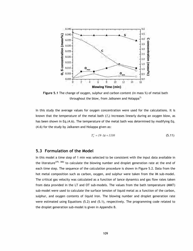
109

Figure 5.1 The change of oxygen, sulphur and carbon content (in mass %) of metal bath

throughout the blow, from Jalkanen and Holappa7)

In this study the average values for oxygen concentration were used for the calculations. It is

known that the temperature of the metal bath (Tb) increases linearly during an oxygen blow, as

has been shown in Eq.(4.6). The temperature of the metal bath was determined by modifying Eq.

(4.6) for the study by Jalkanen and Holappa given as:

1330t19T t

b +∆⋅= (5.11)

5.3 Formulation of the Model

In this model a time step of 1 min was selected to be consistent with the input data available in

the literature379, 380) to calculate the blowing number and droplet generation rate at the end of

each time step. The sequence of the calculation procedure is shown in Figure 5.2. Data from the

hot metal composition such as carbon, oxygen, and sulphur were taken from the IM sub-model.

The critical gas velocity was calculated as a function of lance dynamics and gas flow rates taken

from data provided in the LT and OT sub-models. The values from the bath temperature (MMT)

sub-model were used to calculate the surface tension of liquid metal as a function of the carbon,

sulphur, and oxygen contents of liquid iron. The blowing number and droplet generation rate

were estimated using Equations (5.2) and (5.1), respectively. The programming code related to

the droplet generation sub-model is given in Appendix B.

110

Figure 5.2 Algorithm of droplet generation program

5.4 Results and Discussion

5.4.1 Effect of Operating Conditions

The blowing number was calculated as a function of the gas flow rate, nozzle diameter, lance

height, surface tension, and density of liquid metal, and the results are presented in Figure 5.3.

The lance height is the only variable changing with time, whereas the other parameters of lance

design remain constant in this particular practice. The lance was kept close to the metal bath in

the early part of the blow, followed by an increase in lance height during the main blow. Towards

the end of the process the lance height was decreased again. As can be seen in Figure 5.3, when

the lance height decreased, the transfer of jet momentum from the gas to liquid phase increased

and therefore the blowing number increased.

Figure 5.3 Blowing number as a function of lance height and blowing time354)

Initialize variables Tb, QO2, h, n, dt, α,ρg,

mass % C, mass % O,mass % S

Calculate blowing number, NB

Calculate critical gas velocity, UG

Calculate generation rate of metal droplets

Calculate surface tension of liquid metal, γ

111

The calculated blowing number as a function of lance dynamics ranges from 6 to 8.5. For

example, the maximum value for a blowing number occurs in the initial period of the blow when

the lance height is 0.9 m. The blowing numbers obtained in the present study are consistent with

those obtained by Subagyo et al.252)

5.4.2 Effect of Surface Tension

The effect of the surface tension of liquid iron as a function of temperature and oxygen, and the

sulphur and carbon contents in liquid iron was investigated, and the results are given in Figure

5.4. The surface tension of liquid iron, relative to the surface tension of pure iron, decreases as

the temperature of the bath and oxygen content of the liquid iron increase. Although the

temperature of the bath increases linearly, the surface tension increases due to a decrease in the

sulphur and oxygen concentrations from 11 min to 15 min after the start of the blow.

Figure 5.4 The change of surface tension with time as a function of bath temperature, oxygen,

sulphur and carbon contents

The results of the blowing number calculations as a function of the variations of surface tension

changing with time are given in Figure 5.5 and Figure 5.6. The decrease in surface tension

increases the blowing number with time, particularly for the first four minutes of the blow,

because the lance height remains constant. However, a change in the position of the lance height

has more effect on droplet generation than the change in surface tension.

Figure 5.6 shows the difference between the blowing numbers calculated by considering constant

and variable surface tension throughout the blow. It can be seen from Figure 5.6 that they are

close to each other, which implies that the transfer of jet momentum is the crucial factor for

droplet generation compared to changes in the physical properties of liquid iron in top blowing

112

practice. These calculations were repeated using the maximum oxygen content value presented

in Figure 5.1, and the same conclusion was reached. If blowing parameters such as lance height

and oxygen flow rate remain constant, then variations in the surface tension of liquid iron

become more important.

Figure 5.5 The blowing number and surface tension as a function of time

Figure 5.6 The blowing number determined using constant and varying surface tension

5.4.3 Effect of Carbon Content at the End of the Blow

It is known that oxygen concentration in the liquid metal increases with decreasing the rate of

decarburization at the end of the blow. As more oxygen is dissolved in the metal, the surface

tension will be much lower and more droplets will be generated towards the end of the blow.

This effect was considered for the present industrial data using Equation (5.9). Accordingly, the

113

blowing number as a function of surface tension at the end of the blow was obtained, i.e. the

data point at the 18th min as shown in Figure 5.6. As seen, the blowing number increases to a

higher value at the end of the blow. It can be said that the effect of the surface tension of liquid

metal, and thereby the composition of the liquid iron, becomes more significant towards the end

of the blow.

The relationship between the end carbon and oxygen contents was investigated using Eq.s (5.9)

and (5.10). The end carbon content in liquid metal was selected ranging from 0.25 to 0.01 mass

%, and the corresponding oxygen contents were calculated. The calculated oxygen contents

(along with the bath temperature, the carbon contents and an assumed sulphur content of 0.03

mass %) were then used in considering the change in surface tension for calculating the blowing

numbers prior to the end of the blow. The results of the calculations for different lance height

are shown in Figure 5.7. As the end carbon level of the liquid metal decreases the blowing

number increases for a given lance height. The blowing number increases from 8.3 to 14.5 when

the end carbon level decreases from 0.25 to 0.01 mass % for a lance height of 1 m.

Figure 5.7 The relationship between end carbon content in liquid iron and NB

These findings are important when modelling oxygen steelmaking because it allows the oxygen

content of the bath, a quantity that is difficult to measure and predict, to be largely ignored

when calculating the droplet generation rate with time. In the case of low carbon steels, the

authors suggest that droplet generation becomes more dependent on the composition of steel

required only towards the end of the blow. It should be noted that this result is only based on one

set of industrial data, however, the author expects this finding would be duplicated in similar

industrial studies. Further industrial trials are required to fully quantify this effect.

114

The author also expects the oxygen content at the impact zone to be higher than the bulk oxygen

content in a liquid bath. Therefore, the calculations based on bulk data will tend to

underestimate droplet generation. However, there is no data available in the literature to

quantify this suggestion.

5.5 Conclusion

To establish the effects of the operating conditions and the liquid properties on droplet

generation for a top-blown oxygen steelmaking process, a mathematical model was developed in

this study and the conclusions reached are as follows:

1. The blowing number increases with decreasing the lance height, due to an increase in

the intensity of jet momentum.

2. The surface tension has an influence on droplet generation. Droplet generation during the

blow increases as the surface tension of the liquid metal decreases.

3. We proposed that droplet generation in top blown oxygen steelmaking is mainly

dominated by the blowing conditions, not by the physical properties of liquid metal.

However, the composition of the steel strongly affects the generation of droplets for low

carbon steels towards the end of the blow.

Further studies are required to verify these conclusions, particularly focusing on the simultaneous

effect of temperature and oxygen content on the surface tension of liquid metal, and the

variation of oxygen content in iron during steelmaking.

In summary, the droplet generation rate will be calculated as a function of the blowing

parameters. And the values for the physical properties of metal such as surface tension and

density will be considered as constant in the global model.

115

CHAPTER 6

6 Flux Dissolution Model*

6.1 Introduction

In oxygen steelmaking flux is added to the process in a solid shape to form a basic slag that will

limit the degradation of the refractory lining and remove oxidation products such as phosphorus

and silicon. The progress of flux dissolution determines the efficiency of fluxing the impurities

and prolongs contact time with the refractory lining. Since the top blowing process takes only 15-

20 min to refine impurities from the steel, full utilization of the flux addition requires rapid flux

dissolution in the slag. Therefore, the degree of flux dissolution is of crucial interest for

understanding the progress of slag-metal reactions in the oxygen steelmaking system.

This model was designed to calculate the rate of flux dissolution in the slag phase, which

determined the weight of slag generated for each time step. There have been several

experimental studies302, 304-306, 309-311, 314-317, 381-384) on the mechanism and kinetics of flux addition

into stirred and stagnant slag baths at high temperatures. However, these are generally limited

studies with experimental conditions such as the stirring intensity, composition, and temperature

of the molten slag system which can be practically studied at laboratory scale. Although these

studies provide qualitative information on flux dissolution, it is difficult to apply the findings to

predict the kinetics of flux dissolution under full-scale operating conditions. There have also been

studies385-389) on the dissolution of solid into liquids related to the effects of the mixing

characteristics of liquids induced by gas bubbles for metallurgical systems at high temperatures.

However, the effect of gas generation on flux dissolution has never been reported in literature.

The aim of the present study is to provide a better knowledge on the rate of flux dissolution

under full-scale operating conditions at high temperatures. In the present study the effects of the

composition of slag and stirring intensity induced by CO gas bubbles on the kinetics of flux

dissolution were investigated using a numerical solution of equations and validation of the model

using an industrial study by Cicutti and his co-workers.379, 380) The following specific issues

associated with flux dissolution were also investigated:

(1) the effects of particle size on dissolution

(2) the effects of flux addition rates on dissolution

(*This chapter has been published in a form of journal paper in ISIJ international in October 2009.)

116


In this model the dissolution rate of fluxes vr (m/min), into the slag system was expressed as a

function of the rate of decrease of the thickness of solid flux particles, assuming spherical

geometry.

dt

dr

dt

dV

S

1vr −=−= (6.1)

where vr is the rate of decrease of the thickness of solid particle (m/min), V is the volume of

particle (m3), S is the surface area of particle (m2), r is the radius of particle (m) and t is time

(min).

The number of particles dissolved in the slag is proportional to particle concentration in the slag.

The calculations for different individual particle size were carried out separately and the results

were then added. The amount of lime WL and dolomite WD dissolved in the slag phase as a

function of time was determined using:

LL

L ndt

drSρ

dt

dW= (6.2)

DD

D ndt

drSρ

dt

dW= (6.3)

where ρL is the density of lime (kg/m3) and ρd is the density of dolomite (kg/m3). nL and nD are the

number of lime and dolomite particles, respectively. The total amount of lime dissolved in slag at

time t, tt

Ld,M ∆+ was determined by summation of total amount of lime dissolved at time t and the

amount of lime dissolved at given time step, ∆t (see Eq.6.4). The same calculation procedure was

applied for the total amount of dolomite dissolved at time t using Eq.(6.5).

∆tdt

dWMM Lt

Limed,

tt

Limed, +=∆+ (6.4)

∆tdt

dWMM D∆tt

Dolomited,

t

Dolomited, += − (6.5)

where the subscript d refers to dissolved flux in slag. In this study, the amount of slag formed for

each time step was determined using predetermined CaO content (in mass %) in the slag phase

given by Eq.(6.6).

CaO mass%

M100M

t

CaOd,t

slag

×= (6.6)

117

6.2.1 Rate-Determining Mechanism of Lime Dissolution

In this study the rate of dissolution was assumed to be controlled by CaO diffusion through a

boundary layer.308) The dissolution rate can be calculated by the model suggested by Matsushima

et al.305)

∆(%CaO)100ρ

ρk

dt

dr

L

s=− (6.7)

where ρs is the density of slag (kg/m3) and k is the mass transfer coefficient of CaO in the slag

(m/min). ∆(%CaO) is the difference between the concentration of CaO in the slag phase and its

solubility in the slag phase (in mass %). In this model the solubility of CaO was obtained from the

ternary phase diagram of FeO-SiO2-CaO considering intersections between the liquidus line with a

straight line connecting the point 2CaO.SiO2. In this method the maximum CaO/SiO2 should be the

value on the liquidus line of 2CaO.SiO2 saturated region.390) Details of the calculation procedure

for dissolution mechanism and rate equation of lime are given in Figure 6.1.

6.2.2 Rate-Determining Mechanism of Dolomite Dissolution

In this model the dissolution of dolomite depends on the FeO content of slag phase. The

dissolution rate of dolomite was controlled by the dissolution of CaO through a liquid boundary

layer for slags containing FeO less than 20 mass %.306) The relationship was expressed as

follows:306)

∆(%CaO)ρ100

ρk

mw

mw1

dt

dr

d

s

CaO

MgO

+=− (6.8)

On the contrary, if FeO content of slag is above 20 mass %, the change in the radius of dolomite

particle was calculated using the following correlation:306)

∆(%MgO)ρ100

ρk

mw

mw1

dt

dr

d

s

MgO

CaO

+=− (6.9)

where ∆(%MgO) is the difference between the concentration of MgO in the slag phase and its

saturation in the slag phase (in mass %). In this model the solubility of MgO was determined using

modified relationship for CaO-MgO-FeO-SiO2 slag saturated with magnesiowustite at 1600ºC

reported in literature.390) This relationship was modified by Chen et al.391) They suggested a

relationship between MgO concentration for a given slag composition at 1600ºC and slag

temperature to predict the solubility of MgO at various temperatures. This relationship was

applied in this study to calculate the saturation concentration of MgO. It should be noted that the

dissolution of refractory lining to the system was not considered in this model. Therefore, the

118

model tends to under estimate the total volume of slag. The calculation procedure for dissolution

mechanism and rate equations of dolomite and lime are given in Figure 6.1.

6.2.3 Mass Transfer Coefficient

Previous experimental studies304-306, 309) provide qualitative information for estimating mass

transfer coefficients. However, these values are not applicable in this model due to different

parameters and operating conditions such as shape of solid particles, slag temperature and

stirring intensity. Semi-empirical relationships based on Sherwood, Reynolds and Schmidt

numbers have been widely used to estimate the mass transfer coefficient of different shaped

solids in steelmaking systems under different flow conditions.304-306, 309, 314, 315) The correlation

proposed by Ranz and Marshall392) is:

1/31/2 Sc0.6Re2Sh += (6.10)

This correlation has been widely applied in the literature. However, this correlation is valid for a

low Reynolds number (2<Re<200). Clift et al.393) proposed a correlation for rigid spheres which

can be applied for a high Schmidt number (Sc>200) and 100<Re<2000. The relationship is:393)

3/10.48 Sc0.724Re1Sh += (6.11)

In this model the Reynolds number was related to the particle size and settling velocity of the

particles. The Schmidt number for CaO and MgO can be found as a function of the physical

properties of slag and diffusivities of lime and dolomite lumps. The physico-chemical properties

of slag were calculated from the literature,394, 395) which is described in Appendix C.2.

In the oxygen steelmaking process a turbulent flow occurs in the vicinity of the oxygen lance due

to rising CO gas bubbles during the blow, generated from decarburization. These rising bubbles

generate a circulation flow that accelerates the mass transfer rate of solid particles in the slag.

Accordingly, the Sherwood number can be related to the stirring intensity induced by CO gas

bubbles using:396)

31

41

3

4

402 /

/

s

pCOSc

v

d.Sh

ε+= (6.12)

where εCO is the stirring power (W/kg), dp is the diameter of particle (m) and vs is the kinematic

viscosity of slag (m2/min). Accordingly, Eq.(6.12) directly relates the mass transfer of particles

with the stirring intensity (rather than particle velocity) influencing the mixing phenomena in the

slag-gas-metal slag.308) The stirring power εCO, can be determined as a function of the CO gas

flow rate generated by the decarburization reaction using397)

119

+=

1.46

hP1log

M

TQ14.2ε a

S

SCOCO (6.13)

where QCO is the gas volume flow rate (Nm3/min) generated by the decarburization reaction, Ts is

the temperature of the slag (K), Ms is the weight of the slag (kg), h is the height of the slag (m),

and Pa is the ambient pressure of the system (Pa). The application of the mass transfer

coefficient and stirring power in this model are illustrated in Figure 6.1.

6.2.4 Diffusivity

There is a limited knowledge on the diffusivities of MgO and CaO in oxygen steelmaking slags.

Umakoshi et al.306) applied a dimensionless mass transfer correlation and estimated the diffusivity

of MgO as 1.5x10-5 to 1.8x10-5 cm2/s for FeO-CaO-SiO2 slags (CaO/SiO2=1 and FeO=20 to 70 mass

%). In the case of lime dissolution, Matsushima et al.305) used the diffusivity of CaO for 20 % FeO-

40 % CaO-40 % SiO2 slags of a value of 2.7 х 10-5 (cm2/s). As far as the author knows, these data

are the only available data in literature providing information on the diffusivities of CaO and MgO

for basic oxygen steelmaking slags using the rotating cylinder technique at 1400 °C. In this study

the values for the diffusivities of CaO and MgO were chosen to be 2.7х10-5 and 1.6 х 10-5 cm2/s,

respectively, at 1400°C. The relationship between diffusivity in liquids and temperature and the

viscosity of liquid by the Stokes-Einstein and Eyring equations, was used to calculate the

diffusivities of CaO and MgO for various temperatures.

s

s

µ

T D ∝ (6.14)

Turbulent diffusivity was introduced for turbulent flow conditions and was assumed to be twice

that of molecular diffusivity.308) The diffusivities of CaO and MgO were then determined as a

function of the temperature and viscosity of slag. These diffusivity values were used to calculate

the dissolution rate of lime and dolomite in Equations (6.7), (6.8) and (6.9) as given in Figure 6.1.


In this model a time step of 1 min was selected to be consistent with the input data available in

literature379, 380) to calculate the amount of CaO and MgO dissolved at the end of each time step.

The sequence of the calculation procedure is shown in Figure 6.1. The programming code related

to the flux dissolution kinetic model is given in Appendix C.1.

120

Figure 6.1 Preliminary algorithm of flux dissolution program

6.4 Input Data

The dissolution rate of lime and dolomite was predicted as a function of the stirring intensity, the

physico-chemical properties of slag, the composition of slag, the temperature profile of the

system, and the saturation limits of CaO and MgO using industrial data from the study by Cicutti

and his co-workers.379, 380)

Table 6.1 shows the operating conditions of an oxygen steelmaking process taken from the study

by Cicutti et al.380) Oxygen was introduced into the process through a lance. Bottom stirring was

also applied to enhance the mass transfer rates, particularly towards the end of the blow. 1000

kg of lime and 1700 kg of dolomite were added before starting the blow. The remaining amount

of lime was continuously added during the first 7 min of the blow at a constant rate, whereas the

remaining amount of dolomite was added 7 min after the blow started. It was also assumed that

1200 kg of lime and 1000 kg of dolomite dissolved in the slag at the end of first minute to be

consistent with the industrial data.

No Yes

Initialize variables Tb, Ts, WL, WD, rL, rD

Find out saturation level of CaO and MgO from phase diagram

Calculate slag properties µs, ρs using Eqs (A.7) and (A.3)

Calculate CO gas generation rate, QCO

Calculate diffusivities DCaO and DMgO using Eq. (6.14)

Calculate stirring power, εCO, using Eq. (6.13)

Calculate mass transfer coefficients, kCaO and kMgO, using Eq. (6.11) and (6.12)

Find out dol. dissolution rate

Is FeO<20?

Calculate dissolution rate

use Eq. (6.8)


use Eq. (6.9)

Calculate dissolution rate of lime use Eq. (6.7)

Calculate amount of flux dissolved at time=t

Calculate amount of slag at time=t

121

Table 6.1 Data used for calculations380)

Amount of hot metal charged 170000 kg

Amount of scrap charged 30000 kg

Amount of iron ore charged 1900 kg

Amount of lime charged

1000 kg before starting the blow 6600 kg in the first half of the blow

Amount of dolomite charged

1700 kg before starting the blow 1100 kg in the first half of the blow

Initial diameter of lime particle 0.03 m

Initial diameter of dolomite particle 0.045 m


Oxygen blow 620 m3/min, 6 hole lance

Inert gas (Ar/N2) 2.5-8.33 m3/min through the bottom

Lance height 2.5 m/ 2.2 m/ 1.8 m

Figure 6.2 shows the evolution of slag composition measured during the blow from the study by

Cicutti et al.380) Initially the FeO content in slag increased rapidly. During the main blow the

level of FeO was reduced significantly by carbon in the metal due to a high decarburization rate.

Towards the end of the blow the FeO in the slag built up again as the decarburization rate

decreased. The temperature profile of the bath is also illustrated in Figure 6.2. In this study it

was assumed that it increased linearly from 1350°C to 1650°C for the given industrial practice.

The calculation procedure for the temperature of the bath and slag are given above in Eq.s (4.7)

and (4.8), in sections 4.2.3 and 4.2.4, respectively.

Figure 6.2 Evolution of slag composition and temperature profile of bath with time380)

122


6.5.1 CO Evolution

The generation of CO gas provides a circulation flow in the system. However, some amounts of

CO gas escaped from the slag and left the system. Therefore, the actual amount of CO gas

influencing the stirring power should be investigated.

Thus, the cumulative CO gas produced enhances the void fraction of gas in the emulsion phase.

For high rates of decarburization, particularly during the main blow, the rate of CO gas

generation increases and not all the CO gas can escape from the emulsion. The excessive amount

of CO gas in the emulsion may cause a slopping problem because of the critical height of foamy

slag reached when the bubble plume completely fills the system.308) Therefore, it is important to

predict the height of foamy slag for a better process control of the system. Accordingly, in this

model the critical height of foamy slag was investigated as a function of the different volume

fraction of CO gas in the emulsion.

There are several ways of calculating the height of foamy slag as a function of the physical

properties of the slag and CO gas generation rate reported in the literature.398-402) However, all

these equations give different values for the height of the foamy slag for process conditions. For

simplicity, in this study the height of foamy slag was approximated by:402)

)φA(1ρ

Mh

gs

s

f −= (6.15)

where hf is the height of foamy slag (m), A is the slag area (m2), and gφ is the gas fraction in

emulsion.

The predicted foam height of an oxygen steelmaking process as a function of the volume fraction

of CO gas held up in the emulsion during a blow is given in Figure 6.3. In this calculation the CO

gas generation rate was obtained from the evolution of the carbon content in the metal bath as a

function of time, where we assumed that all the carbon was converted to CO gas (see Figure 6.2).

The volume fraction of CO gas varied between 5 and 100%. If we assume that more than 10 vol %

of CO gas is held up in the emulsion, the predicted height of the slag exceeds that and might

cause slopping. (i.e.>5 m) The values of foamy height calculated on the basis of a 10 vol % CO gas

assumption lay at the edge of slopping. This finding implies that only a small proportion of the CO

gas generated was held up in the emulsion. In this study we assumed that 90% of the CO gas

generated at any time by-passes the emulsion region (i.e. leaves close to the lance) and the 10%

of CO gas contributes to foaming and stirring the emulsion. Subsequently, all the calculations

123

reported were carried out based on the assumption of 10 vol % of CO gas generated being held up

in the emulsion.

Figure 6.3 Comparison of slag height as a function of volume of CO gas available in the emulsion

during the blow

6.5.2 Determination of Mass Transfer Coefficient

An earlier study305) was carried out at laboratory scale with a defined geometry where the

velocity profile was known. This is not the case in an oxygen steelmaking furnace where the

velocity fields are complex, not homogenous, and not known (e.g. some parts of the slag are

comparatively stagnant). In this study two approaches were compared, (a) assuming the velocity

is simply the settling velocity, and (b) using a correlation for turbulent flow induced by gas

bubbling. This methodology is outlined in Figure 6.1 and described in an earlier section called the

“Mass Transfer Coefficient”. Accordingly, different correlations were used to determine the

appropriate mass transfer correlation for calculating the dissolution rate of lime and dolomite

particles in the slag. The mass transfer coefficient of sphere particles under laminar and

turbulent flow conditions was determined using Equations (6.11) and (6.12), respectively. The

results for the weight of undissolved lime were compared with those reported by Cicutti et al.

given in Figure 6.4.

The measured values for the industrial practice lie between those values from two different

assumptions. A laminar flow assumption under predicts the dissolution rate but even using only 10

% CO gas generated to stir the emulsion over predicts the dissolution. Therefore, the author

suggests there are two different flow regimes in the slag due to the stirring conditions. The

regime near the lance has a higher stirring intensity due to the generation of CO gas. This regime

124

can be called “turbulent”. The regime further away from the lance and close to the refractory

lining is expected to be a more stagnant regime. Therefore, the dissolution of solid particles in

this stagnant regime takes place at a slower rate compared to that in the turbulent regime.

Figure 6.4 Comparison of the weight of undissolved lime as a function of time between predicted

values by assuming laminar and turbulent flow and those reported by Cicutti et al.167)

The flow regime in the furnace was defined due to the Reynolds number as a function of the

settling velocity of solid particles. In the early part of the blow the values for the Reynolds

number lie in the transient regime (100<Re<500). However, as the particles become smaller,

their movement is faster and the flow becomes more turbulent. It is concluded that it is not

possible to model flux dissolution using one simple correlation to understand the complex nature

of the oxygen steelmaking process. As a practical solution to the problem we introduced a

constant (β) to modify the settling velocity of the particles and provide a means of modelling the

data. The correlation by Clift et al.393) was modified using the following relationship:

( ) 3/10.48ScRe'0.7241Sh += (6.16)

s

spp

µ

ρduβReβ'Re == (6.17)

where up is the settling velocity of particles and dp is the diameter of solid particle. Accordingly,

the weight of undissolved lime as a function of β were calculated and compared with those

reported by Cicutti et al. given in Figure 6.5. The predicted amount of undissolved lime for β=10

is more closer value for the measured value of undissolved lime in the slag from the study by

Cicutti et al.379) This implies that the stirring effect of CO gas on the dissolution rate is crucial

and should be related to determine the mass transfer coefficient. It may also be necessary to

125

model the emulsion region as a multi-zoned reactor to reflect stirring near the lance, as

compared to the wall region. The CFD model may also be useful to study the variation in flow

conditions around flux particles, as a function of the changing process conditions. The

recommended value of β is 10 for all practical applications to predict the overall dissolution rate

of lime and dolomite for oxygen steelmaking. The algorithm to model the dissolution of flux in

the emulsion for β=10 is illustrated in Figure 6.6.

Figure 6.5 Comparison of the weight of undissolved lime as a function of different β values with

those reported by Cicutti et al.379)

The author would prefer not to introduce this factor but introducing β is practical and

particularly useful to steelmakers. It should be noted that this limitation aside, this study is the

most scientifically rigorous treatment of flux dissolution available in the literature.

6.5.3 Evolution of the Amount of Slag

The flux dissolution model using Equation (6.16) for β=10 was validated using the study by Cicutti

et al.379) Figure 6.7 shows the results of changes in the slag weight during the blow compared

with those reported by Cicutti et al.379) Both the measured silicon content in the metal and slag

phase during practice, and flux additions to the process, were used to estimate the slag weight.

The results of these calculations for slag weight are illustrated as Sample 1 and Sample 2 in

Figure 6.7. Initially (between 2-4 min), the slag weight increases linearly and remains constant

during the time between 5-12 min but towards the end of the blow, it increases linearly. The

maximum and minimum values of slag weight with time, as estimated by Cicutti et al. are shown

in Figure 6.7. The results for the predicted slag weight from the flux dissolution model for β=10

were consistent with data from the study by Cicutti et al. However, during the main blow (5-12

min), values for the weight of the slag are relatively higher than previous results.

126

Figure 6.6 Algorithm of flux dissolution program incorporating β (The broken box shows the

modified steps)

Figure 6.7 Comparison of model results for the weight of slag with those reported by Cicutti et

al.167) during the blow

Yes

Initialize variables Tb, Ts, WL, WD, rL, rD

Find out saturation level of CaO and MgO from phase diagram

Calculate slag properties µs, ρs using Eqs (A.7) and (A.3)

Calculate Re number using Eq. (6.17)

Calculate diffusivities DCaO and DMgO using Eq. (6.14)

Calculate mass transfer coefficients, kCaO and kMgO, using Eq. (6.16)

Find out dol. dissolution rate

Is FeO<20?


use Eq. (6.8)


use Eq. (6.9)

Calculate dissolution rate of lime use Eq. (6.7)

Calculate amount of flux dissolved at time=t

Calculate amount of slag at time=t

No

127

6.5.4 Effect of Particle Size on Dissolution

The effect of the size of solid lime and dolomite particles on the dissolution of lime and dolomite

was investigated using the mass transfer correlation given in Equation (6.16) for β=10. Three

different sizes for lime (0.06 m, 0.04 m and 0.02 m) and dolomite particles (0.09 m, 0.06 m and

0.03 m) were selected in this model. Figure 6.8 and Figure 6.9 show predictions for the amount

of lime and dolomite dissolved in the slag as a function of various particle sizes. Decreasing the

size of lime particles from 0.06 m to 0.04 m increases the dissolution of lime from 4300 kg to

5460 kg. Solid lime is present in the slag at the end of the blow regardless of particle diameter.

In the case of dolomite, particles with a diameter of 0.03 m dissolved completely at the end of

the blow. Solid dolomite remained at the end of the blow when the sizes of the particles were

0.06 m and 0.09 m. As a result, as the size of the solid particles decreased, the amount of flux

dissolved increased simultaneously.

Figure 6.8 The predictions of amount of lime dissolved with respect to initial size of lime

particles

6.5.5 Effect of Addition Rate of Flux on Dissolution

The effect of the flux addition rate on the kinetics of flux dissolution was investigated. The

dissolution rate of lime and dolomite were also calculated using the mass transfer correlation

given in Eq. (6.16) for β=10. Different addition rates for lime and dolomite are given in Table 6.2.

In Case 1 and 3, it was assumed that 1000 kg of lime and 1700 kg of dolomite were added before

starting the blow. The remaining amount of lime and dolomite was added continuously during the

first 3 minutes of the blow at a constant rate in Case 1. In Case 2, both the amount of dolomite

and lime charge was increased to 2000 kg prior to the blow. The remaining amount of lime and

dolomite was added continuously during the first 7 minutes of the blow at a constant rate, for

128

Case 2 and 3. The results of the weight of lime and dolomite dissolved in the process are given in

Figure 6.10 and Figure 6.11, respectively.

Figure 6.9 The predictions of amount of dolomite dissolved with respect to initial size of lime

particles

Table 6.2 Different flux additions for top blowing oxygen steelmaking

lime addition dolomite addition stages

Case 1 1000 kg prior to blow 1700 kg prior to blow

3

6600 kg in the early blow 1100 kg in the early blow


7



7


With the dissolution of lime and dolomite, an increase in the addition of lime and dolomite prior

to the blow increases the amount of lime and dolomite dissolved in the slag. When flux particles

are added continuously in 3 min, a higher dissolution of lime would be achieved than a constant

addition in 7 min. This might be due to the higher concentration difference of CaO and MgO that

accelerates the dissolution of CaO and MgO during the process. As a result, the faster the flux

addition is the more flux is dissolved in the system.

129

Figure 6.10 Predictions for lime dissolution as a function of various addition rates of lime

These findings are important for the oxygen steelmaking process because it provides crucial

information on the progress of flux dissolution that affects the refining reactions and physical

properties of the slag. Accordingly, this model can be used for better process control for a top

blowing oxygen steelmaking process.

Figure 6.11 Predictions for dolomite dissolution as a function of various addition rates of

dolomite

130

6.6 Conclusion

The models for lime and dolomite dissolution as a function of temperature, slag composition, and

stirring intensity were developed for oxygen steelmaking slags at high temperatures. The models

provide a better understanding of crucial factors affecting the dissolution of fluxes, and allow for

quantitative predictions of flux dissolution. The following conclusions can be drawn from the

present study:

- The oxygen steelmaking process has heterogenous mixing characteristics. In the beginning, solid

particles exist in a transient regime with regard to their size and velocities. As the particles

decrease in size, those that remain in the turbulent regime become faster. Therefore, it is

difficult to predict the dissolution rate of solid flux particles using one simple equation. To

incorporate the stirring effect with laminar flow conditions a modified correlation was proposed

for practical reasons. The recommended value for β is 10.

- The flow rate of stirring gas has a crucial impact on the rate of dissolution of flux additions. The

increase in gas flow rate gives a higher mass transfer rate.

- The decreasing size of particles of lime and dolomite can effectively promote their dissolution

in oxygen steelmaking slags.

- Increasing the addition rate of lime and dolomite both prior to and during a blow increases the

amount of flux dissolved in the slag. If the lime addition occurs in three stages rather than seven,

a greater amount of lime would dissolve in the early part of the blow which would affect the

characteristics of slag such as viscosity and fluidity, and would also reduce the slag attack on the

refractory lining.

As a summary, the flux dissolution rate will be calculated based on the laminar flow assumption

for β=10. And the weight of slag will be calculated as a function of the amount of CaO dissolved

in the process with time in the global model.

131

CHAPTER 7

7 Scrap Melting Model

7.1 Introduction

Scrap is a raw material used in the oxygen steelmaking process. The progress of scrap melting is

important because it has a crucial impact on the carbon concentration and temperature of the

steel. The presence of unmelted scrap at the end of the blow might cause re-blows with their

numerous problems such as the over-oxidation of metal and slag, and disruption of metal flow in

the plant.288, 297) Therefore, it is important to understand the fundamentals of scrap melting in

the oxygen steelmaking process.

The kinetic model developed by Sethi et al.284) was applied in this study because it was relatively

easier to apply compared to the other available models.297, 300) The mathematical model applied

an analytical solution technique using industrial data taken by Asai and Muchi.298) This model was

further modified to be applicable for other sets of industrial data. The model outlined below is

designed to calculate the melting rate of scrap, and thereby the amount of scrap melted at a

given temperature with each time step. This information will be linked to the global model to

find out the overall mass balance of the furnace.


The melting rate of scrap v (m/s), into liquid iron was expressed as a function of the rate of

decrease of the thickness of solid scrap particles,284)

t

Lv

∆∆

= (7.1)

In reality it is hard to assume the geometry of scrap charged because it is left over parts of the

goods. For simplicity it was assumed to be plate in this study. Accordingly, the amount of scrap

melted in the metal bath as a function of time was determined using:284)

Avdt

dWSc ρ= (7.2)

7.2.1 Rate-Determining Step

It is established that both mass and heat transfers are crucial to the melting rate of scrap.

However, there is still a debate in the literature on the rate limiting step of scrap melting. The

models285, 288, 297) are proposed based on various assumptions.

132

In this model, for the sake of simplicity, the carbon concentration of the metal bath was assumed

to be equal to the carbon concentration at the interface. It was also assumed that the bath

temperature is relatively higher than the scrap temperature at the interface. Under these

conditions, heat transfer control was considered to be the rate-limiting step. The melting rate of

scrap v (m/s), into liquid iron was obtained using an equation for the conservation of heat at the

solid-melt interface, which can be written as:283, 288)

( ) ( )int

sc

Fe

'

bx

TAvHATThA

∂

∂λ−∆−ρ=− (7.3)

where h is the heat transfer coefficient, λ is the heat conductivity, A is the surface area of scrap

and ρ is the density of scrap. The enthalpy change in scrap melting and raising the temperature

of liquid metal to interface temperature is equal to ∆HFe. This relationship is given using:

( )'TTCphH bmFe −+∆=∆ (7.4)

Based on the conservation of heat, the heat flux supplied from the liquid metal was used for the

absorption of heat into the cold scrap and the melting of the scrap.

7.2.2 Calculation of Interface Temperature

The temperature at interface T', was related to the interface carbon concentration referring to

the Fe-C phase diagram using:

'C'T 901810 −= , %.'C 2740 ≤≤ (7.5)

1425='T , %.'C 274>

Here C' and T' denote the carbon concentration and the scrap temperature at the interface. The

temperature of the bath (Tb) was assumed to increase linearly during the oxygen blow as shown in

previous studies.76, 298)

7.2.3 Calculation of Scrap Temperature

For one dimensional heat flow the temperature distribution across the scrap at a given time step

can be obtained by employing the Fourier series using:284)

∑∞

==

αλ−π

=∂

∂

1

2

02

n

n

x

Sc )texp(L

nA

x

)t,x(T

(7.6)

In Eq. (7.6), it was assumed that n is 3 and An is the coefficient of Fourier series. In this study the

temperature distribution of the scrap was estimated and calculated using the error function,

133

which is simple to apply and valid for calculations over short time steps.149) The temperature

profile of the scrap can also be predicted using:

[ ]

[ ]

++⋅+++

−+⋅+−

+

++

−−=

−

−

Fo2

x/L1FoBierfcFoBix/L)Bi(1exp

Fo2

x/L1FoBierfcFoBix/L)Bi(1exp

Fo2

x/L)(1erfc

Fo2

x/L)(1erfc1

TT

TT

2

2

biSc,

bSc

(7.7)

where the half thickness of the scrap and the thickness of the scrap from the centreline of the

scrap are represented by L and x, respectively. In this calculation procedure the Biot number (Bi)

and Fourier number (Fo) were obtained using:149)

hL/λBi = (7.8)

2αt/LFo = (7.9)

The Biot number expresses the ratio between the surface conductance and interior thermal

conductivity of a body whereas the Fourier number is the ratio of the heat conduction rate to

thermal heat storage rate.149)

7.2.4 Boundary Conditions

The process of scrap melting can be broken into three stages, Solidification takes place on

surface of the scrap if the heat flux transfer from the metal bath is smaller than heat conduction

in the scrap. The Solidified shell melting stage continues until the thickness of the scrap returns

to the initial value. The normal melting stage continues until all the scrap is melted. The

mathematical descriptions of the boundary conditions were given in the following equations.283,

284)

Solidification occurs while ( )x

TTTh Sc'

b ∂

∂λ<− (7.10)

Solidified shell melting occurs while 0LL ≥ (7.11)

Normal melting occurs while 0L ≥ (7.12)


In this model a time step of 1 s was selected to predict the scrap melting rate at the end of each

time step. The computational set-up of the model is illustrated in Figure 7.1. The input data was

taken from the IM and IS sub-models.

134

Figure 7.1 Algorithm for scrap melting model

Heat convection was calculated as a function of the bath temperature and interface temperature

of scrap; whereas heat conduction was calculated as a function of the interface temperature of

scrap-metal, scrap temperature, and thermal conductivity of the scrap. The heat convection and

heat conduction were compared. If the heat conduction is much higher than heat convection,

solidification takes place. Conversely, melting takes place. The melting rate of scrap was

estimated using Equation (7.3), the energy conservation equation. The calculations are

programmed in Scilab and the details of the program code are given in Appendix D.

No

Yes

Initialize variables Tb, TSc, WM, WSc, rSc,Cm, CSc

Calculate interface temperature using Eq.(7.5)

Find out carbon concentration at interface

Calculate scrap temperature using equation, Tsc

Calculate Tav, CpSc, λSc

Work out melting stage: Is heat

conduction>heat convection?

Calculate heat convection

Calculate heat conduction use Eq. (7.6)

Calculate melting rate of scrap at time t

Calculate thickness of scrap at time t

Melting occurs

Solidification occurs

Calculate amount of scrap dissolved at time t

135

7.4 Input Data

The input data influencing the kinetics of scrap melting are the weight, temperature, and the

composition of hot metal and scrap, the size of scrap particles, the oxygen flow rate, and the

decarburization rate. The shape of the scrap also influences its melting rate, however, different

shaped scrap was not considered in this model.

Table 7.1 shows the operating conditions of oxygen steelmaking process taken from the industrial

data in the study of Sethi et al.284) Changes in the carbon concentration of steel are presumed

from the same set of industrial data.

Table 7.1 Data used for calculations284)

Amount of scrap charged, kg 8000

Initial hot metal temperature, K 1573

Initial scrap temperature, K 303

Bulk carbon concentration, mass % 4.26

Area of scrap/liquid interface, m2 5.4

L, scrap thickness, m 0.2

h, heat transfer coefficient in liquid metal, W/m2K 3630

Scρ , density of scrap, kg/m3 7200

∆h, heat of fusion, kJ/kg Fe 277.2

α, thermal diffusivity of scrap, m2/s 0.0000062

7.5 Validation of the SD Model

The melting rate of scrap was calculated as a function of the temperature profile of the scrap

and carbon concentration of the metal bath. The heat transfer coefficient was assumed to be

constant. Enthalpy changes in the scrap can be found using Equation (7.4). Figure 7.2 compares

the values of scrap thickness as a function of time predicted by the modified model, with the

study by Sethi et al.284) The results agreed with the previous study and are applicable for other

industrial applications. It should be noted that the heat transfer coefficient should be modified.

Heat transfer coefficients can be estimated from experimental studies using a dimensionless

analysis technique.285, 403) However, this approach is not likely to be valid for oxygen steelmaking

where the velocity fields are complex and not homogenous (e.g. some parts of the slag near the

136

furnace walls maybe comparatively stagnant). The difficulty in measuring velocity fields in

steelmaking furnaces compounds the problems because validation is very challenging.

A dimensionless analysis technique has been applied widely to calculate the heat transfer

coefficient under forced convection. Specht and Jeschar404) developed a relationship for different

types of solid particles (range of validity 0Pr ≥ ). Szekely et al.285) suggested that the heat

transfer coefficient can be related with stirring intensity under steelmaking operating conditions.

The values for the heat transfer coefficient lie between 3500 and 11800 W/m2K. Gaye et al.288)

also performed some plant scale experiments to determine the melting time of scrap in top-

blown, bottom-blown, and combined blown processes. The suggested value for the heat transfer

coefficients is 17000 W/m2K for a 310 t top-blown process.288) The heat transfer coefficient

should be modified based on the stirring conditions in industrial practice. Irons et al.405, 406)

studied scrap melting behavior using computation fluid dynamics for electric arc furnace

steelmaking. The heat transfer model was based on phase field modelling proposed by Li et al.283,

407) This model can predict the stirring effect of the melting of individual solid scrap particles but

this modelling technique is not currently incorporated into the global model due to its

complexity.

Figure 7.2 The change in scrap thickness as a function of time

7.6 Conclusion

The scrap melting model developed by Sethi et al.284) was modified to include variations in the

heat transfer coefficient and error function for calculating the temperature of scrap. The model

allows quantitative predictions of scrap melting for industrial practices. However, it should be

137

noted that this model should be checked against other sets of data and is an area worthy of

further investigation.

As a summary, scrap melting can be calculated as a function of the temperature, the particle size

of the scrap for oxygen steelmaking process at high temperatures, and will be linked to the global

model to calculate the overall mass balance in the furnace.

139

CHAPTER 8

8 Decarburization in the Emulsion Model

8.1 Introduction

One of the main goals of the oxygen steelmaking process is to effectively reduce the carbon

concentration of the liquid iron. It is understood that most carbon removal reactions occur in the

emulsion phase via a reaction between the metal droplets and slag phase.170, 172) An improved

understanding of this reaction and the factors controlling the overall rate should provide a better

control of the process and increase productivity. In the literature there is a limited knowledge of

how to relate the carbon removal rate within droplets to the overall kinetics of the process under

full scale operating conditions. This chapter will focus on a development of the decarburization

reaction in the emulsion phase that incorporates the droplet residence model.


In the emulsion zone a decarburization reaction takes place via an FeO reduction given in

Equation (2.56). The theoretical treatment suggested by Brooks et al.151) was applied in this study

to estimate the decarburization rates of metal droplets as a function of the dynamic changes in

their behavior. Using this approach the total decarburization rate in the emulsion zone can be

obtained from a summation of the decarburization rates of individual metal droplets as a function

of droplets volume due to a bloating behavior of the droplets. In the model the metal droplets

were ejected with rate RB to the slag phase, the generated droplets, whose residence time was

smaller than the given time-step, returned from the emulsion zone at rate RD. When the steady

state conditions were reached, droplet generation rate was equal to the droplet returning rate.

The droplet generation rate can be obtained using a blowing number, as explained in Chapter 5.

The rate of metal droplets returning to the metal bath with respect to residence time tr can be

written as:

≥

<=

ijBi

ij

Di tr∆tR

tr∆t0R

(8.1)

Here i represents the ejected time of the metal droplets and j represents the blowing time of the

process. Because all the droplets ejected at each time step were assumed to have the same

residence time for a defined size droplet, the mass of metal droplets in the emulsion with

respect to the residence time tr can be written as:

140

≥

<=

ijijBi

ijBi

Bi tr∆ttrR

tr∆t∆tRV

(8.2)

The mass of metal droplets returning is the remaining mass of droplets generated after the

decarburization reaction. It can be calculated by substituting the quantity of carbon removed

from the quantity of metal droplets ejected at time i. The relationship is given as:

( )

≥−

−

<= ∆+

ij

t

i

tt

ii

Bi

ij

Ditr∆t

100

CCm∆tR

tr∆t 0

V

(8.3)

where mi is the weight of a single droplet (kg). Thus the decarburization rate can be calculated

using:

( )t

CC100

m

dt

dW

t

i

tt

i

m

1i

i

C

∆

−

=

∆+

=∑

(8.4)


The transport of oxygen through the slag phase or bubbles surrounding the metal droplet, the

transfer of carbon in the metal, interface chemical reaction, nucleation and removal of CO gas

bubbles from the reaction site may all be important in determining the rate of the

decarburization reaction. However, there is no agreement in the literature on the rate

controlling step of this reaction under various operating conditions, as discussed in section

2.4.1.2.

Variation in the carbon content of a single droplet was calculated using different rate equations

suggested by previous researchers to determine a rate controlling step for the decarburization

reaction within metal droplets. Table 8.1 summarizes the previous studies with given rate

equations and suggested reaction mechanisms. These studies were compared because they were

developed for slags containing high concentrations of FeO which are valid for oxygen steelmaking

slags. The input data for this comparison was taken from the previous experimental study by

Molloseau and Fruehan240) because the experimental conditions were well defined and valid for

oxygen steelmaking operating conditions.

In the reaction rate equation proposed by Molloseau and Fruehan240), ks refers to the mass

transfer coefficient in the slag phase, mwFeO is the molecular weight of FeO, mass % FeO is the

FeO content of bulk slag, mass % FeOs is the FeO content at the surface of a droplet, and A refers

to the surface area of an emulsified droplet determined by the observation of x-ray videos. In the

reaction rate equation suggested by Brooks et al.5), keff is the mass transfer coefficient in the

141

metal droplet, Aapp is the apparent surface area of the droplet, Vapp is the apparent volume of the

droplet, mass % C is the carbon content in a droplet, and mass % Ceq is the equilibrium carbon

content. In Chen and Coley’s equation236), ne is the number of molecules in an embryo, NA is

Avogadro number, and V0 is the original droplet volume. Js is the nucleation rate and can be

found using:236)

( ) ( )[ ]

−

ψσπ−

π

ψσ

∆−=

2

Lve

3

0

2/1

00s

PPkT3

16exp

m

3

kT

HexpNJ (8.5)

where N0 is the number concentration of CO embryos in the liquid, σ0 is the surface tension at

liquid gas interface, ∆H is the heat of formation of one CO molecule, m is the mass of one

molecule, T is the temperature, k is the Boltzman constant, Pve is pressure in the vapour bubble

at equilibrium, PL is the liquid pressure, and ψ is the reduction magnitude of surface tension.

Table 8.1 Comparison of previous studies on decarburization in emulsion

Studies Rate Equation Mechanism

Molloseau and

Fruehan240)

( )s

FeO

ss FeO%massFeO%massmw100

Ak

s

molesRate −

ρ=

mass transfer of FeO

through slag phase

Brooks et al.5) ( )eq

app

app

eff C%massC%massV

Ak

s

%massRate −=

mass transfer of carbon

through metal phase

Chen and

Coley236) ( )0V

N

nJ

s

molesRate

A

e

s=

chemical reaction of C and

O in the metal droplet

Figure 8.1 presents changes in the carbon content of a metal droplet as a function of time. The

kinetic model proposed by Brooks et al., based on a simple surface renewal model of carbon

diffusion, closely follows the measured values of the carbon content in the droplet. It is

important to note that the Brooks et al. model used empirical data from the Molloseau and

Fruehan study for some of the parameters in their model, so in effect they “fitted” their model

to the data and only claimed that this model is useful for global kinetic calculations and not

necessarily the “correct” kinetic model. Carbon diffusion with the metal droplets might be the

rate controlling step for the bloated droplets because there is enough oxygen available in the

system so that the generation rate of CO gas is high and the metal droplets become bloated.

Nevertheless, further work is required to fully understand the mechanism at the individual

droplet level.5) The approach of Brooks et al. was successfully applied to the experimental

results240) and this approach was incorporated into the global model.

142

Figure 8.1 Comparison of the change in carbon content of a metal droplet between measured

values from the experimental study of Molloseau and Fruehan240) and proposed kinetic models

As reviewed in section 2.4.2, other impurities such as silicon and manganese have an impact on

the decarburization rates of metal droplets in oxidizing slag. It should be noted that the

experimental studies169, 233) were limited with high manganese and silicon content, which were

relatively higher (above 1 mass %) than those in oxygen steelmaking practice. Only the model

developed by Sun and Zhang233) considered the metal droplets containing low silicon and

manganese content (below 1 mass %). In their work it was predicted that the decarburization

reaction rate was also suppressed and the effect of impurities was lower. However, these

predictions were not validated against experimental or industrial data. In conclusion, other

impurities have a potential to decrease the decarburization rates of metal droplets in the slag.

Particularly, high silicon could cause the formation of SiO2 at the start of the blow that retards

the decarburization reaction. There is very limited data available in the literature on the effect

of impurities on decarburization. Additionally, the industrial data used in this study has no

information about impurities within the metal droplets. For simplicity, it was assumed that

droplets only contain carbon and the effects of other impurities were not included.

In this model the effective mass transfer coefficient keff was calculated on the basis of Higbie’s

penetration theory.408) When the volume of an element is carried from a liquid phase to the

interface it reaches a stagnant point where it allows a certain concentration of the substance to

penetrate from the other phase before returning to its original liquid phase. This theory assumes

143

that the surface is continuously renewed by this process. The diffusion boundary layer can be

related to the residence time of the element at the interface. This approach was employed by

Brooks et al.5) to predict the mass transfer coefficient of carbon to the interface based on the

residence time of dense and bloated droplets. The relationship is:

p

dC

effD

uD2k

π= (8.6)

where DC is the diffusivity of carbon and ud is the overall velocity of droplet estimated by:

2

z

2

rd uuu += (8.7)

Here, uz and ur are the velocity of a metal droplet in the vertical and horizontal directions,

respectively. The calculation procedure of these values will be explained in the following section.

8.2.2 Droplet Residence Model

The decarburization rate is strongly dependent on the residence time of droplets in the emulsion,

as mentioned above, and that the bloating of a droplet is critical to understand the overall

kinetics of steelmaking. This model was designed to calculate the residence time of metal

droplets ejected to the emulsion phase as a function of the physical properties of slag, the FeO

concentration of slag, the carbon concentration of metal, and droplet generation due to jet

intensity.

The model developed by Brooks et al.5) was applied in this study because it includes the dynamics

of the motion of droplets in the slag-gas-metal emulsion phase. In the proposed model a force

balance was made based on the ballistic motion of a single droplet at vertical and horizontal

coordinates. The motion of a single droplet is illustrated in Figure 8.2.

Figure 8.2 The schematic illustration of ballistic motion of a metal droplet in slag5)

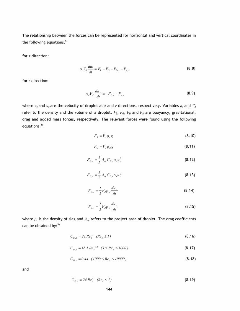
144

The relationship between the forces can be represented for horizontal and vertical coordinates in

the following equations.5)

for z direction:

z,Az,DGB

z

dd FFFFdt

duV −−−=ρ (8.8)

for r direction:

r,Ar,D

r

dd FFdt

duV −−=ρ (8.9)

where uz and ur are the velocity of droplet at z and r directions, respectively. Variables ρd and Vd

refer to the density and the volume of a droplet. FB, FG, FD and FA are buoyancy, gravitational,

drag and added mass forces, respectively. The relevant forces were found using the following

equations.5)

gVF sdB ρ= (8.10)

gVF ddG ρ= (8.11)

2

zsz,Ddpz,D uCA2

1F ρ= (8.12)

2

rsr,Ddpr,D uCA2

1F ρ= (8.13)

dt

duV

2

1F z

sdz,A ρ= (8.14)

dt

duV

2

1F r

sdr,A ρ= (8.15)

where ρs is the density of slag and Adp refers to the project area of droplet. The drag coefficients

can be obtained by:5)

1

zz,D Re24C −= )1(Rez ≤ (8.16)

6.0

zz,D Re5.18C −= )1000Re1( z ≤≤ (8.17)

44.0C z,D = )10000Re1000( z ≤≤ (8.18)

and

1

rr,D Re24C −= )1(Rer ≤ (8.19)

145

6.0

rr,D Re5.18C −= )1000Re1( r ≤≤ (8.20)

44.0C r,D = )10000Re1000( r ≤≤ (8.21)

where

s

spz

z

DuRe

µ

ρ= and

s

spr

r

DuRe

µ

ρ= (8.22)

Here Dp is a diameter of droplet and µs is the viscosity of slag. The velocity of the droplet to be

inserted into the Reynolds number was related to the initial velocity of metal droplet.

Substituting Equations (8.10) through (8.15) into Equations (8.8) and (8.9), the velocity of

droplets at z and r directions can be obtained in the following.5)

2

z

d

p,d

ds

z,Ds

ds

dsz uV

A

2

C

2

g)(2

dt

du⋅

ρ+ρ

ρ−

ρ+ρ

ρ−ρ= (8.23)

2

r

d

dp

ds

r,Dsr uV

A

2

C

dt

du⋅

ρ+ρ

ρ−= (8.24)

Equations (8.23) and (8.24) are the major differential equations to be solved. These equations

are highly non-linear. A numerical calculation was undertaken using the explicit forward

differencing method. The finite difference equations of (8.23) and (8.24) were derived as:

( ) ( ) ( )2

zz0

zz 1iu1iKKt

1iu)i(u−−+=

∆

−− (8.25)

( ) ( ) ( )2

rr

rr 1iu1iKt

1iu)i(u−−=

∆

−− (8.26)

Here

ds

ds

02

g)(2K

ρ+ρ

ρ−ρ= and

( ) dds

r,Ds

rD22

C3K

ρ+ρ

ρ−= (8.27)

Finally, the trajectory of a droplet in various directions can be calculated using the numerical

values of uz and ur:5)

[ ]∑ ∆−+=i

zzz t)1i(u)i(u2

1)i(L (8.28)

[ ]∑ ∆−+=i

rrr t)1i(u)i(u2

1)i(L (8.29)

146

where Lz(i) and Lr(i) are the trajectories of a droplet trajectory at z and r directions, respectively.

∆t is time-step used in differential equations. As Lz(i) approaches zero, the residence time can be

estimated using:5)

∑∆=

i

ttr (8.30)

This model is called the “ballistic motion model” and is valid for dense droplets. Dense droplets

can be seen under conditions of weak decarburization rates. In order to calculate the residence

time of bloated droplets the threshold decarburization rate was calculated. The bloating behavior

phenomenon cannot yet be completely explained from basic principles, so empiricism was

introduced. As a consequence, the threshold decarburization rate was evaluated from an

experimental study by Molloseau and Fruehan240) and calculated as a function of the FeO content

in slag using:5)

( )FeO%mass1086.2r 4*

c

−×= (8.31)

Subsequently, the apparent density of a droplet can be calculated as a function of the initial

density and rate of decarburization reaction given by:5)

c

c

0ddr

r ∗

ρ=ρ (8.32)

where ρd0 is the initial density of a droplet cr is the decarburization rate, and ∗cr is the threshold

decarburization rate. If there is no bloating motion of a droplet its apparent density is equivalent

to its initial density. It is represented as:5)

0dd ρ=ρ (8.33)

8.2.3 Basis of the Model

The following assumptions have been made in the model based on the industrial data available

for a 200-t oxygen steelmaking furnace.

1) The factors affecting the path of decarburization are the temperature profile of hot metal, the

amount of hot metal charged, hot metal and scrap compositions, scrap and flux additions, and

blowing practice, which were considered as system inputs for this model given in Figure 8.4. The

input data for the calculations were taken from industrial data reported by Cicutti et al.166, 167)

The outcome of other refining reactions such as the FeO concentration was entered as known

variables.

2) The simultaneous decarburization reactions at the impact zone and in the emulsion zone,

temperature profile of the bath, the dissolution process of flux, the melting process of scrap, the

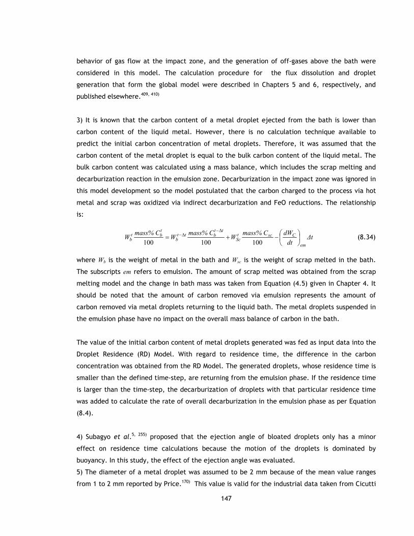
147

behavior of gas flow at the impact zone, and the generation of off-gases above the bath were

considered in this model. The calculation procedure for the flux dissolution and droplet

generation that form the global model were described in Chapters 5 and 6, respectively, and

published elsewhere.409, 410)

3) It is known that the carbon content of a metal droplet ejected from the bath is lower than

carbon content of the liquid metal. However, there is no calculation technique available to

predict the initial carbon concentration of metal droplets. Therefore, it was assumed that the

carbon content of the metal droplet is equal to the bulk carbon content of the liquid metal. The

bulk carbon content was calculated using a mass balance, which includes the scrap melting and

decarburization reaction in the emulsion zone. Decarburization in the impact zone was ignored in

this model development so the model postulated that the carbon charged to the process via hot

metal and scrap was oxidized via indirect decarburization and FeO reductions. The relationship

is:

∆tdt

dWmass% CW

mass% CW

mass% CW

em

CsctSc

ttbtt

b

tbt

b

−+=

∆−∆−

100100100 (8.34)

where Wb is the weight of metal in the bath and Wsc is the weight of scrap melted in the bath.

The subscripts em refers to emulsion. The amount of scrap melted was obtained from the scrap

melting model and the change in bath mass was taken from Equation (4.5) given in Chapter 4. It

should be noted that the amount of carbon removed via emulsion represents the amount of

carbon removed via metal droplets returning to the liquid bath. The metal droplets suspended in

the emulsion phase have no impact on the overall mass balance of carbon in the bath.

The value of the initial carbon content of metal droplets generated was fed as input data into the

Droplet Residence (RD) Model. With regard to residence time, the difference in the carbon

concentration was obtained from the RD Model. The generated droplets, whose residence time is

smaller than the defined time-step, are returning from the emulsion phase. If the residence time

is larger than the time-step, the decarburization of droplets with that particular residence time

was added to calculate the rate of overall decarburization in the emulsion phase as per Equation

(8.4).

4) Subagyo et al.5, 255) proposed that the ejection angle of bloated droplets only has a minor

effect on residence time calculations because the motion of the droplets is dominated by

buoyancy. In this study, the effect of the ejection angle was evaluated.

5) The diameter of a metal droplet was assumed to be 2 mm because of the mean value ranges

from 1 to 2 mm reported by Price.170) This value is valid for the industrial data taken from Cicutti

148

et al. They also stated that the drop size varies from 0.23 mm to 3.35 mm.166) However, the

effects of size distribution on the instanenous decarburization rates in the emulsion phase and

overall kinetics of the process were included.

6) The decarburization rate of an individual droplet was calculated using the rate equation

proposed by Brooks et al. given in Table 8.1.

7) The diffusivity of carbon in liquid iron is 2х10-9 m2/s at 1600 °C.411) The diffusivity of carbon

was determined as a function of the slag temperature and viscosity of the slag-metal-gas

emulsion based on the Stokes-Einstein and Eyring equations for various temperatures. It was

assumed that the slag temperature increases linearly and is 100°C higher than the bath

temperature. The relationship is given in Equation (4.8) in Chapter 4.

8) For a slag-metal-gas emulsion, the motion of metal droplets is influenced by the gas bubbles

trapped in the gas phase. The metal droplets were treated as a dispersed phase in a slag-gas

continuum. The average density and viscosity of the slag-gas continuum was calculated by the

following equations.5, 257)

( )gsggsg φρφρρ −+= 1 (8.35)

( )( )( )gs

gsg

g

ssg ρρ

ρρ

φ

µµ

−

−

−=

3/113

2 (8.36)

Here gφ refers to the volume fraction of the gas in the emulsion and can be given by:5)

smg

sg

VVV

V

++=φ (8.37)

Initially, the density and viscosity of slag was calculated as a function of the slag composition and

temperature as explained in Appendix C. These values were entered as input data into the

droplet residence model. The average density and viscosity of the slag-gas continuum were

calculated as a function of the gas volume, as given in Equations (8.35) and (8.36) to predict the

velocity of the droplets in the z and r directions.

9) The initial velocity of a droplet was estimated based on the conservation of energy relationship

proposed by Subagyo et al.255) This relationship suggests that the kinetic energy of blown gas is

used to generate and eject the droplets. The kinetic energy absorbed by a metal droplet from the

oxygen jet EKd was calculated using:255)

149

2

)0(dBKd uR2

1E = (8.38)

where RB and ud(0) denote the droplet generation rate and initial velocity of droplets,

respectively. This relationship is valid if all the produced droplets are spherical. The kinetic

energy of the blowing gas EKg, is:255)

2

gGgKg uR2

1E ρ= (8.39)

The kinetic energy absorbed by the metal droplets was correlated to the kinetic energy of blown

gas as a function of the blowing number NB based on the experimental data reported by Subagyo

et al.255) and Koria and Lange.267) The correlation is given in the following255)

7.0

B

Kg

KdN00143.0

E

E= (8.40)

10) The equilibrium concentrations of carbon and iron oxide were determined by the activity

coefficient and concentration. The activity of carbon follows Henry’s Law and was calculated

from the interaction parameter of carbon itself because it was assumed that carbon is the only

substitute in a metal droplet. Alternatively, the Raultian activity coefficient of iron oxide was

determined as a function of the temperature and composition of other oxides in slag. The

programming codes for the equilibrium calculations are given in Appendix E.

11) Ito and Fruehan412, 413) reported that the gas volume fraction in the slag-metal-gas emulsion

varies between 0.7 and 0.9. The average value of this range, 0.8, was used to calculate the slag-

gas continuum in this study. An assessment of this assumption will be discussed in the results

section.

12) The slag foam height was assumed to be constant and equal to 2 m. In an oxygen steelmaking

furnace the foam height might reach to the mouth of the furnace, particularly during the main

blowing period. An assessment of this assumption will be discussed in the results section.


The sequence of calculation procedure to compute the residence time of metal droplets ejected

for a given time step is shown in Figure 8.3. Blowing conditions such as the variation in lance

height and presumed slag composition were entered as input data into the RD sub-model. The

slag properties were calculated as a function of the slag composition and temperature. The

droplet generation was then calculated as a function of blowing conditions. The output results of

150

the droplet generation sub-model were used to calculate the initial velocity of metal droplets

ejected to the emulsion phase and calculate the quantity of metal droplets ejected. Then, the

velocity and trajectory of metal droplets were obtained based on the finite difference technique.

The values of droplet velocity as a function of change in their diameter were put into an Equation

(8.6) to calculate the effective mass transfer coefficient. Therefore, the decarburization rate in

the metal droplets and change in the carbon concentration of metal droplets can be calculated.

If the decarburization rate is higher than threshold decarburization, bloating occurs. This

calculation procedure was repeated until the trajectory of metal droplets in the z direction

reaches zero. The programming code related to the droplet residence model is given in Appendix

E. In this droplet residence model the selected time step was 0.0001s for numerical accuracy and

computational time.

The sequence of the calculation procedure to estimate the decarburization rate of metal droplets

is shown schematically in Figure 8.4. The programming code is provided in Appendix F. The

output values for residence time and change in carbon content of metal droplets were taken from

the RD sub-model to feed into the DCE sub-model as input data.

The matrix called “DrTime” was introduced to track the change of the residence time of metal

droplets ejected from the liquid bath in each time step, with respect to blowing time. The

residence time of metal droplets were entered into the matrix beginning with time=2 min.

corresponding to the moment they were ejected to the slag phase.

The matrix DrTime is given using:

( ) ( ) ( )( ) ( )

( )

=

ttr000

......00

ttr...ttr0

ttr...ttrttr

DrTime

ij

j222

j11211

M,....,1j

M,.....,1i

=

= (8.41)

ttrtr 1ijij ∆−= − (8.42)

The matrix DrTime is an M×M array where M is the total number of time steps for a single

simulation. In the proposed global model the time-step ∆t was selected as 1 min and the process

time step is divided into N equal small time-steps ∆ts=∆t/N. For example, if the time step is

selected as 5 seconds for DCE sub-model then ∆ts would be 5 and N would be equal to 12. For the

entire blowing time, the total amount of variables, M to be entered to the matrix can be found

using:

151

Figure 8.3 Algorithm of droplet residence model

NtM b ×= (8.43)

Here tb denotes the blowing time. Another matrix called “Crange” was formed which denotes the

change in carbon concentration with respect to blowing time. This matrix was developed based

on the same procedure as the “DrTime” matrix.

Yes

Initialize variables Tb, Ts, WM, dd, QO2, h, n, dt, α

Calculate blowing number, NB

Calculate slag properties µs, ρs u

Calculate generation rate of metal droplets

Calculate initial velocity of droplet with size of dd

Find out decarburization rate

Is rc<rc*?

Calculate threshold decarburization rate, rc*

Calculate density change

No

Calculate velocity of droplet with size of dd

Calculate mass transfer coefficient

Calculate decarburization rate

Calculate diameter change

Calculate carbon content in metal droplet

Calculate residence time of droplet

Calculate trajectory of droplet

152

( ) ( ) ( )( ) ( )

( )

=

tC000

......00

tC...tC0

tC...tCtC

Crange

ij

j222

j11211

M,....,1j

M,.....,1i

=

= (8.44)

Both matrices, DrTime and Crange could then be used in the program to estimate the total

amount of metal droplets in the emulsion phase, the total amount of metal returning to the

metal bath, and the total decarburization rate of metal droplets in the emulsion phase.

Based on droplet residence, the quantity of metal droplets in the emulsion phase and quantity of

metal droplets returning to the metal bath were calculated using Equations (8.2) and (8.3),

respectively. And the total decarburization rate within the individual droplets was calculated

using Equation (8.4).

Figure 8.4 Algorithm of the decarburization model

8.4 Verification and Validation

The droplet residence sub-model was verified by comparing the predicted droplet residence time

by the model with the results of Brooks et al.5) Figure 8.5 shows the position of droplets ejected

at a 60 deg angle as a function of the initial droplet diameter. The calculations were performed

based on a 2 m thick layer of slag with a density of 2991.4 kg/m3 and a viscosity of 0.0709 Pa.s.

The model was able to duplicate the previous model. This model was linked to decarburization in

the emulsion model.

Initialize variables WM, dd, Ci,

Calculate residence time of metal droplets

Calculate slag properties µs, ρs u

Calculate decarburization rate using Eq.(8.4)

Calculate carbon content of metal droplets using Eq.(4.4)

Get values from Droplet Residence Model

153

Figure 8.5 The results for the residence time of metal droplets with various diameters as a

function of vertical distance are compared with Brooks et al.5)

The decarburization rate was calculated based on an assumption that the decarburization

reaction only takes place in the emulsion zone. Industrial data from the study by Cicutti et al.166,

167) was used as an input in this model. The operating conditions are given in Table 8.2. The

model predictions for the carbon content of liquid iron with respect to various time steps are

given in Figure 8.6. The results are close to each other. A comparison of the decarburization rate

in the emulsion zone as a function of various time steps is given in Figure 8.7. The rates predicted

by the model are converging as the time step decreased. The results for 5 and 2 s time steps are

close to each other until 12 min after the start of the blow. Later, periodical differences can be

seen towards the end of the blow. This is due to the presence of dense droplets in the emulsion

phase. Towards the end of the blow, metal droplets contain less carbon and the driving force for

the reaction between metal droplets and slag is decreased. The bloating behavior of droplets

only takes a short time due to weak decarburization and the emulsion phase begining to collapse.

Unfortunately, calculations for the decarburization rate of dense droplets did not converge

because the time step was reduced. In order to overcome this numerical problem it was

necessary to run the routine using very short time steps (<0.5 s). However, the calculations could

not proceed for smaller time-steps due to computational limitations. For this reason, the results

presented were based on the model using 5 s time-steps.

It should be noted that these numerical problems had no noticeable influence on the overall rate

of carbon removal in the emulsion, as mention in section 8.2.3. The mass balance calculation

only considers the amount of carbon removed from the metal droplets returning to the bath. For

instance, the maximum difference in the total amount of carbon removed is approximately 25 kg

154

for a 2 s time step, which decreases to 0.1 kg towards the end of the blow. At peak points after

12th min, as seen in Figure 8.7, the difference in the amount of carbon removed increased to 15

kg. However, these “spikes” in the instantaneous decarburization rates are not important to the

overall rate of carbon removal. These results show that whilst the current model is not good at

predicting instantaneous decarburization rates for dense droplets, this is not a major shortcoming

for predicting the overall decarburization rate.

Table 8.2 Data for numerical calculation166, 167)

Hot metal charged 170 t

Scrap charged 30 t



Number of nozzle 6

Throat diameter of nozzle 33 mm

Exit diameter of nozzle 45 mm

Inclination angle 17.5°



Tapping temperature 1650 °C

Figure 8.6 Model predictions for carbon content of liquid iron were compared for various time-

steps with respect to blowing time

155

As seen in Figure 8.7, the model predicts that the decarburization rate increases at 4 min and at

7 min. At this point the rate reaches its peak level during the main blow and decreases back

towards the end of the blow. This increase in the decarburization rate is due to variations in the

lance height. These variations in lance height were given in Figure 8.7. As the lance height is

decreased there is an increase in the number of droplets ejected through the emulsion zone and

consequently, the reaction rate of decarburization increases significantly in the emulsion zone.

Figure 8.7 Model predictions for decarburization rate in the emulsion phase were compared for

various time-steps as a function of lance height


8.5.1 Residence Time

Figure 8.8 illustrates the evolution of the residence time of droplets with a diameter of 2 mm as

a function of the carbon concentration of the bath, as predicted by the proposed model. In the

early part of the blow the residence time of droplets is around 45 s. Towards the end of the blow

it decreases to 0.4 s. As seen, the residence time of droplets is much higher in the presence of

high carbon concentrations. Towards the end of the blow the residence time is low due to weak

decarburization rates. This may imply that the metal droplets are “bloated” with CO gas,

156

generated during the active decarburization period and then become less dense and spend longer

time in the emulsion.206) However, towards the end of the blow the metal droplets maintain their

original density due to slow decarburization.


droplets

Significant differences in droplet residence time are also due to the physical properties of slag as

a function of the gas volume fraction. For example, the gas hold up of 80% in the emulsion

increases the viscosity of the slag-gas continuum by two times the viscosity of the slag, and

decreases the density of the slag-gas continuum by four times the density of the slag. Model

results of residence time, assuming a gas volume fraction of 0.8 with respect to the density and

the viscosity of slag-gas continuum, are illustrated in Figure 8.9.

The residence times of droplets decrease as the density of the slag-gas continuum decreases

towards the end of the blow. On the other hand, it is expected to observe a higher residence

time because the viscosity of the slag-gas continuum decreases. As the carbon content of droplets

decreases the droplets are not bloated and have a short residence time. This demonstrates that

the carbon content of liquid iron has a predominant role on the residence time of droplets.

A significant decrease in the residence time of droplets decreases the decarburization rates as

per that given in Figure 8.7. As a result, it was concluded that the decarburization rate is strongly

dependent on the residence time of droplets in the emulsion and that the bloating of a droplet is

critical to understand the overall kinetics of steelmaking. It was found that running the model

without including the bloated droplet theory (every droplet is dense) results in vastly under

predicting the overall decarburization rate. The decarburization rate via emulsified droplets

decreases from 200 kg/min to 70 kg/min when dense droplet assumption was considered.

157

Figure 8.9 Evolution of droplets residence time with respect to physical properties of slag-gas

continuum during the blow

8.5.2 Effect of Gas Fraction on Residence Time

Figure 8.10 shows the residence time of bloated droplets in the slag-metal-gas emulsion

predicted for different volume fractions of gas hold up. It can be seen from these results that the

greater the hold up of gas in the slag, the shorter the predicted residence time of the droplets.

As the gas volume fraction increases from 0.7 to 0.9, the residence time of droplets is predicted

to decrease from 45 s to 0.9 s. This variation is due to a change in the physical properties of the

slag-gas continuum. Particularly, the variation in viscosity has a greater impact on the residence

time of the droplets. The residence time of droplets will decrease from 51 s to 0.6 s as the

viscosity of the slag-gas continuum increases from 26.02 kg/ms to 28.175 kg/ms, if the volume

fraction of gas increases from 0.7 to 0.9.

A further instance of this is that the density of the slag-gas continuum varies between 450 and

550 kg/m3 for a gas fraction of 0.8. This range will decrease approximately 250-270 kg/m3 for a

gas fraction of 0.9. As the gas hold up increases the density decreases and the viscosity increases,

which in turn, influences the velocity of the droplets and thereby the trajectory of the droplets.

As a result, the droplets return to the bath in a shorter time. This implies that the amount of gas

in the emulsion is crucial to accurately predict the residence of droplets.

The presence of gas in the emulsion depends on the bloating behavior of the droplets as well as

gas generated from the impact zone. Since the decarburization reaction in the impact zone has

been ignored at this stage, the amount of gas generated in the emulsion was calculated as a

158

function of the gas generated within the metal droplets using Equation (8.37). The change in the

gas fraction is given in Figure 8.11. As seen from the results presented, the gas fraction is

relatively smaller than those reported in the literature. This implies that some of the gas

generated from the impact zone is also held up in the emulsion phase. However, it is very

difficult to estimate this process variable due to the lack of data in the literature. Therefore, the

gas volume faction will be considered as constant and equal to 0.8 in this study.

Figure 8.10 Residence time of the droplets as a function of gas fraction

Figure 8.11 Gas fraction in the emulsion during the blow

8.5.3 Effects of Ejection Angle on Residence Time

The droplet residence model was further used to investigate the effects of the ejection angle on

droplet trajectories under various operating conditions. Table 8.3 lists the selected operating

conditions such as variations in the lance height and FeO concentrations of the slag taken from

industrial data by Cicutti et al. at various blowing periods, to investigate the effects of different

process conditions on the behavior of metal droplets.

159

Table 8.3 Measured FeO concentration and lance variations taken from the industrial data166) at

different blowing period

mass % FeO

Lance height

Ejection time from start of the blow min sec

Early blow 31.3 2.5 m 3 00

Main blow 17.5 2.2 m 8 00

End blow 23.5 1.8 m 15 00

Figure 8.12 illustrates the model’s predicted trajectories of metal droplets at z and r directions

as a function of the ejection angle. The ejection angle has no influence on the vertical distance

that droplets can reach for that particular blowing period. The model predicts that the metal

droplets could not reach the top of the slag and the maximum height predicted varies as a

function of the blowing period. The highest point in the z direction predicted is 0.25 m which is a

relatively short distance from assumed height of the slag foam.

Figure 8.12 Trajectories of metal droplets with different ejection angles at various blowing

periods

160

8.5.4 Effects of Droplet Size on Residence Time

Figure 8.13 illustrates the change in the size of a droplet ejected at a 60° angle from the bath

predicted by the global model as a function of residence time during the blow. There is a

significant increase in diameter (three times larger than initial diameter) of a droplet due to its

bloating behavior regardless of the blowing period. However, this increase in size decreases

towards the end of the blow. This is most likely due to a decrease in the carbon concentration

because the decarburization rate decreases with a decrease in the carbon concentration of the

droplets. This indicates that maximum decarburization will be achieved initially followed by an

eventual decrease in the reaction rate. The carbon content of the droplet and concentration of

FeO are important in determining changes in the size of the droplet. However, the effect of

variations in FeO content in the slag is not clear in this study. Therefore, a more robust

understanding of how FeO varies during the blow will be important to improve the models

described in this study because the FeO values used in our calculation come directly from

industrial data.

Additionally, slag formation has an influence on the prediction of droplet residence times.

However, it is unlikely the current study will investigate any further because the model does not

include slag formation. The effect of slag formation on the droplets residence time is also worthy

of further study.

Figure 8.13 Change in diameter of droplets ejected in a 60-deg angle at different times

predicted by the model

161

Figure 8.14 illustrates the model’s predicted residence time of bloated droplets ejected at a 60˚

angle with respect to different droplet sizes in various ejection periods. The droplet residence

time varies significantly with respect to the operating conditions as well as droplet size. In an

early blow, as droplet size increases, the residence time increases. It is most likely that the

metal droplets contain more carbon and they require a longer time for the decarburization

reaction. The droplets with an initial diameter of 0.25 mm are predicted to return quickly due to

fast decarburization in the early and main blowing period.

In addition, the blowing conditions also influence the distribution of residence time for different

size droplets. In the main blow, the residence time first increases with the initial diameter of the

droplets and then decreases for droplets initially larger than 1 mm. A similar behavior was

obtained for droplets initially larger than 0.5 mm towards the end of the blow. It can be

concluded that maximum residence time shifts from larger droplets to smaller ones as the carbon

concentration decreases.

Figure 8.14 Residence times predicted by the model for industrial data by Cicutti et al. as a

function of droplet size at different blowing period

The trajectory of droplets with various droplet size ejected at a 60° angle at various ejection

times was compared with respect to time in Figure 8.15. It shows that larger droplets are

predicted to spend a longer time than smaller droplets in the emulsion, except at the end of the

blow. In the early blow the droplets are thrown higher than those ejected during later stages of

the blow. It can be noticed that the droplets with an initial diameter of 3 mm return to the bath

immediately since the ejection velocity is more likely to become low towards the end of the

162

blow. On the other hand, droplets with an initial diameter of 0.25 mm return to the bath zone

directly, due to fast decarburization. This implies that the residence time of droplets decreases

significantly, which in turn lowers the decarburization rates, particularly towards the end of a

blow.

Figure 8.15 Behavior of droplets ejected at different times predicted by the model

8.5.5 Effects of Droplet Size on Decarburization Rate

Figure 8.16 illustrates the changes in decarburization rates as a function of droplet size with

respect to blowing time. As discussed in Figure 8.14 and Figure 8.15, the residence time of larger

droplets is higher than smaller ones in the early blow where in turn the decarburization rates will

increase as the droplet size increases. Later, the decarburization rates of large droplets

decreases dramatically compared to the reaction rates of smaller ones. This shows that the

decarburization rate strongly depends on the residence time of droplets. Additionally, the model

suggests that the maximum reaction rates in the emulsion can be achieved by the generation of

smaller droplets.

163

Once again, this figure indicates that the model cannot predict the decarburization rates of

dense droplets towards the end of a blow, as mentioned in section 8.4. Metal droplets 2 mm or 3

mm in size become dense and only spend a few seconds in the emulsion phase compared to the

smaller ones. Mathematically, the decarburization rates of the present dense droplets add up

with those of bloated droplets which in turn, generate noticeable differences in the overall

decarburization rates in the emulsion phase. These differences are relatively small for smaller

droplets because they are bloated and contribute to the carbon refining rates in the emulsion

phase.

Figure 8.16 Model predictions of decarburization rates as a function of droplet size

8.5.6 Effect of Ejection Angle on Decarburization Rate

Decarburization in the emulsion model was simulated for a 30° and 60° ejection angle to verify

this assumption. The simulations were performed for droplets with an initial diameter of 2 mm.

Figure 8.17 demonstrates the change in the decarburization rate predicted by the model as a

function of the ejection angle. As seen from the figure, the decarburization curves are close to

each other during the first half of the blow because the metal droplets are bloated. The model

predicts that the decarburization rates using an assumption of droplet ejection in a 60° angle are

relatively lower than those with a 30° ejection angle. It would seem that the decarburization

rate decreases as the ejection angle increases towards the end of the blow. This implies that as

the droplets become denser the ejection angle has more influence on their residence time.

In this study the decarburization rates were calculated based on an assumption that the ejection

angle is constant and equals 60°, as mentioned in section 8.2.3 for simplicity. This assumption

seems to be reasonable since the metal droplets become bloated during most of the blow.

164

Figure 8.17 Model predictions of decarburization rate with respect to ejection angle

8.6 Conclusion

A mathematical model was developed to study the decarburization reaction in the slag-metal-gas

emulsion for industrial practice. A numerical calculation technique was used to predict the

residence time of the droplets and the decarburization rates of individual droplets during the

blow. This model was linked to the global model to calculate the carbon change of a metal bath

with time. As a result of decarburization in the emulsion model, the following conclusions can be

drawn.

1. The bloated droplet theory has been applied to the industrial data. A global model including

the bloated droplet theory can predict the decarburization rates of individual droplets under full-

scale operating conditions for the oxygen steelmaking process. The decarburization rate in the

emulsion zone increases as the lance height is decreased.

2. The proposed model provides information about variations in the residence time of ejected

metal droplets. For bloated droplets, it is predicted that their residence time in emulsion is

around 45 s during the blow. Towards the end of the blow, the residence time of droplets

decreases to 0.4 s.

3. The residence time of droplets depends strongly on the carbon content of the metal droplets

as well as the volume fraction of the gas in the slag-metal-gas emulsion.

165

CHAPTER 9

9 Decarburization in the Impact Zone Model

9.1 Introduction

The model described in this chapter was designed to calculate the rate of decarburization in the

impact zone for a given time step. There have been several experimental studies on the

mechanism and kinetics of the decarburization reaction of liquid iron with gaseous oxygen and

carbon dioxide. However, there are only limited studies58) based on the industrial data of carbon

removal rates via direct oxidation at the impact zone, due to the complexity of the process. This

model is an attempt to implement the theoretical findings from experimental studies to full-scale

operating conditions.


At the impact zone the dissolved carbon reacts with gaseous oxygen and carbon dioxide. (See

section 2.5) The reactions are:

[ ] )g()g(2 CO2COC =+ (9.1)

[ ] )g()g(2 COO2/1C =+ (9.2)

Accordingly, the decarburization rate via CO2 and O2 are given by the following equations,

respectively.8)

2CO

C JV

Amw100

dt

dC

ρ=

− (9.3)

2

200 OC JV

Amw

dt

dC

=

−ρ

(9.4)

where A is the surface area, V is the volume of the liquid, ρ is the density of liquid metal and mwC

is the molecular weight of carbon. 2COJ and

2OJ are the flux of carbon dioxide and the flux of

oxygen with regard to the Equations (2.52) and (2.53).


In this study it was considered that the decarburization reactions in the impact zone vary over a

large range of temperature and fluid flow conditions, with different concentration of sulphur.

166

In the case of decarburization via CO2, a model based on mixed control kinetics, including gas

phase mass transfer and chemical kinetics, was used because it has been established that sulphur

has a retarding effect on the kinetics of a decarburization reaction60, 155, 161, 195) and this effect

should be considered when investigating the reaction rates of decarburization under various

operational conditions. The rate equation can be written by:60)

b

COa 2Pk

V

A1200

dt

dC

ρ=

− (9.5)

where

tgf

ak/1k/RT

1k

+= (9.6)

Here kg, kt and ka are the gas phase mass transfer coefficient, the chemical rate constant and the

apparent rate constant, respectively. b

CO2P is the partial pressure of CO2 in the gas mixture, R is

gas constant and Tf is the average gas film temperature.

It was assumed that the rate of decarburization via oxygen was controlled by mass transfer in the

gas phase because it has been established that gas diffusion has a predominant effect on reaction

kinetics and surface active elements play no important role on the reaction mechanism.159, 180, 185,

190) The rate equation can be written using:180, 185)

( )b

Og 2P1lnk

V

A2400

dt

dC+

ρ=

− (9.7)

Equations (9.5) and (9.7) were applied to calculate the reaction rates during the blowing period

where the carbon content is high. Below a critical value, carbon diffusion in the liquid phase is

considered to control the reaction rates of decarburization. The rate equation is represented in a

mass unit by the Equation (9.8):154)

( )eqbm

mC C%massC%mass

100Ak

dt

dW −

ρ= (9.8)

where ρm is the density of liquid iron and km is the mass transfer coefficient of carbon in liquid

iron. The equilibrium carbon content, Ceq was small and neglected in the calculations.

9.2.2 Calculation of Rate Constants

There are few studies154, 156, 414-417) for impinging gas jets at the metal surface. Based on the study

by Rao and Trass,414) Sain and Belton154) suggested a mass transfer correlation for impinging a jet

onto a liquid surface.

167

09.0

t

53.006.1

d

'zScRe026.0Sh

−

= (9.9)

This correlation is valid for ( ) 5.6d/'z t ≤ , ( ) 5.4d/x t ≤ but it is not the case in an industrial

configuration. Lohe417) also suggested mass transfer correlations for gas side mass transfer, which

are given based on the range of Reynolds number:

330510411 .. ScRe.Sh = , 42 103102 ⋅≤≤⋅ Re (9.10)

530750410 .. ScRe.Sh = , 54 102103 ⋅≤≤⋅ Re (9.11)

Here D/rkSh 0m= , µρ= /urRe 0 and ( )D/Sc ρµ= . dt refers to nozzle throat diameter and z'

denotes the distance of the nozzle from the surface of the liquid. Interdiffusivity, viscosity and

density of fluid (gas) at Tf are D, µ and ρ, respectively. Sc varies between 0.1 and 2 for gases.149)

These correlations were used for the range of Reynolds number applying in this study. The

velocity of the gas to be inserted into the Reynolds number was designated as the mean velocity

of the gas. In this study it was assumed to be equal to the impact velocity from the oxygen lance.

The details of impact velocity calculation were explained in Chapter 5.

Variable r0 is the radius of the inundated surface area. The variable r0 was considered to be the

radius of the individual penetration area. There are few proposed correlations44, 46, 54, 418, 419) to

calculate the diameter of the penetration area. The correlation developed by Koria and Lange54)

was used to estimate the diameter of the cavity because this study was based on an experimental

study at steelmaking temperatures, and the penetration correlations have been widely used by

many researchers. The relationship was provided in Equation (2.14) in Chapter 2.

According to Sain and Belton154, 155) and Nagasaka and Fruehan,420) the rate constant of the

dissociative adsorption of CO2 for γ-iron by CO-CO2 was:

r

ss

f

t k)S%mass(K1

kk +

γ+= (9.12)

where kf, kr, Ks and γs refers to the chemical rate constant for pure iron, the residual rate at high

sulphur contents, the adsorption coefficient of sulphur, and the activity coefficient of sulphur in

liquid iron, respectively. In the study by Nagasaka et al.420), the standard state for sulphur

activity was taken as 1 mass % in carbon-saturated liquid iron that the activity coefficient was

assumed to equal unity for carbon-saturated liquid iron. The rate constants kf, kr and the

adsorption coefficient, Ks can be calculated as a function of the temperature using:155, 420)

168

21.0T

5080klog f −−= (9.13)

75.1T

5600klog r −−= (9.14)

57.0T

3600Klog s +−= (9.15)

In the case of mass transfer in the metal phase, the mass transfer coefficient was related to the

stirring intensity in the metal bath. Several researchers61, 246, 421, 422) proposed a correlation

between the mass transfer constant to the gas flow rate for gas stirred liquid-liquid systems.

Accordingly, the mass transfer coefficient can be found using:8, 271)

2/1

GCm

A

FDβk

⋅= (9.16)

where β is constant and equal to 500 m-0.5.271) FG is the volumetric gas flow rate (m3/s) and it was

assumed that inert gas blowing from the bottom of the furnace influences mixing in the bath. Dc

is the diffusion coefficient of carbon and the relationship between diffusivity in liquids and the

temperature and viscosity of liquid by the Stokes-Einstein and Eyring equations was used to

calculate the diffusivities of carbon in liquid iron for various temperatures.

9.2.3 Calculation of Partial Pressure

A determination of the partial pressure of oxidizing gasses such as CO2 and O2 is crucial because it

governs the amount of gas delivered to the system in order to achieve reactions at the impact

zone. The partial pressure of gases in the system varies as a function of the reaction rates and

gas composition. In this model it was assumed that the amount of gas blown (O2 and Ar-N2) and

10% of the total amount of gas generated from the decarburization reaction were available in the

impact zone for a given time interval. The gas generated by the decarburization reaction via

emulsion was not included in the calculations of partial pressure of gasses in the impact zone. In

this model the total amount of gas available in the system was calculated by the summation of

gasses (O2, CO, CO2 and Ar-N2) in the unit of mol over time step. The partial pressure of CO2 and

O2 were calculated from the molar rates of Ar-N2 (NA), O2 (NO2), CO (NCO) and CO2 (NCO2) and the

average pressure in the bath (P):

PNNNN

NP

22

2

2

OACOCO

CO

CO ×

+++= (9.17)

169

PNNNN

NP

22

2

2

OACOCO

O

O ×

+++= (9.18)

9.2.4 Calculation of Gas Temperature

The average gas film temperature Tf, is the mean of the temperature of bulk gas and

temperature at the gas-liquid interface. The film temperature was estimated using:185)

( )2

TTKT

bg

f

+= (9.19)

In this study the temperature of CO2, Tg was assumed to be equal to the temperature of the

impact zone whereas the temperature of O2 was assumed to be 25°C. Koch et al.78, 79) suggested

that the temperature at the impact area increases very rapidly in the early blow and remains at a

maximum level during the active decarburization period. Towards the end of the blow the impact

area temperature disappears. According to these studies, the impact temperature was assumed

to be 2000°C until 4 min after the start of the blow, followed by an increase to 2500°C till 14 min

after the blow, and then decreasing to the bath temperature towards the end of the blow, in this

study.

All dimensionless groups, and thereby the mass transfer coefficients of CO2 and O2 were

calculated at the film temperatures of the related gasses, as per previous studies179, 185) whereas

the rate constants kf, kr and adsorption coefficient Ks were calculated at the impact temperature

of the process.

9.2.5 Calculation of the Impact Area

It is known that an increase in the impact area significantly increases the reaction rates.195, 358)

Zughbi195) studied experimentally the effects of the bath surface area on the kinetics of the

decarburization reaction of Fe-C melts using a crucible technique at 1450 °C. They found that a

decrease in the bath area lowers the reaction rates. They observed that the reaction also takes

place outside the penetration area. However, there is limited knowledge of the reaction area at

the impact zone due to difficulties in measurements and visualization at high temperatures.

In this study the penetration area was assumed to be the reaction area for the carbon removal

reaction. The multi-head lance creates individual cavities on the liquid bath. The total impact

area of a jet can be calculated by a summation of the individual areas of a multi-head lance.8)

The shape of the cavity was assumed to be paraboloid.46, 358) The individual impact area was

calculated using:

170

( )i1i

2

i1i

i1i

i

r

0

2

22

rrrr

hh1r2

drdr

dh1r

2

dhdrr2Area

−

−

−+π=

+π=

+π=

++

+∑

∫

∫

(9.20)

where h is the paraboloid height and r is the paraboloid radius. The height equals to the

penetration depth which can be calculated using Korea and Lange’s363) relationship given in

Equation (2.13) in Chapter 2. Similarly, the radius was equal to half of the penetration diameter

and was also taken from Koria and Lange.54) There would also be a change in the cavity

throughout the blow due to surface waves, but this effect was ignored, based on the findings

from a study by Cheslak et al. because the cavity oscillations did not affect the final result of

their observations.46)

9.2.6 Calculation of the Critical Carbon Content

Different proposals were made to determine the critical carbon content of liquid iron. Goldstein

and Fruehan82) defined the critical carbon content as the carbon content where the

decarburization reaction rate during the main blow equals the decarburization rate at the end of

the blow. In this study this approach was used and it was assumed that the point where the total

rate of decarburization via gases was equal to the decarburization rate controlled by the mass

transfer of carbon in the liquid iron. The critical carbon content was obtained using:

( )ρ

ρ++

ρ=

Ak

PkV

A12P1lnk

V

A24

Cm

b

COa

b

Og

cr

22

(9.21)

9.2.7 Calculation of the Physical Properties of Gas

Viscosity

The viscosity of gases can be estimated using the Lennard-Jones parameter. The relationship is

given:423-426)

µ

−

Ω×

××=µ

2

c

fg7

gd

Tmw1093.266 (9.22)

where the molecular weight of gas is expressed as mwg and the collision diameter of gas is as dc.

The collision integral can be approximated by424)

171

2145.0

5.0kTkT

147.1

−−

µ

+

ε+

ε

=Ω (9.23)

In this equation a molecule’s kinetic energy is represented by kT while the potential energy of

two colliding molecules is represented by ε, which is Lennard-Jones potential well depth. The

characteristic parameters ε/k and dc for O2, CO, and CO2 are were taken from the literature427)

and given in Table 9.1.

Table 9.1 Characteristic parameter of gases427)

Characteristic parameters O2 CO CO2

ε/k 113.2 110.3 190

dc, (10-10 m) 3.433 3.59 3.996 Diffusivity

The Chapman-Enskog theory was applied to predict the inter-diffusivity of gases as a function of

temperature. The relationship is:149, 427)

BAAB,D

2

AB,c

2/3

f

ABmw

1

mw

1

dP

T0018583.0D +

Ω××= (9.24)

where the collision diameter between gases can be found using:149, 424)

( )B,cA,cAB,c dd5.0d += (9.25)

The collision integral for mixtures can be approximated by Cloutman424) using:

2

AB

145.0

AB

AB,D 5.0kTkT

−−

+

ε+

ε=Ω (9.26)

5.0

BAAB

kkk

εε=

ε (9.27)


The sequence of calculating decarburization in the impact zone model is shown in Figure 9.1. The

data from hot metal composition such as carbon and sulphur, oxygen flow rate, lance height, and

bottom gas flow rate with time were taken from the related sub-models. The penetration area

was calculated as a function of lance dynamics and gas flow rates.

172

The values from the bath temperature (MMT) sub-model were used to calculate the gas film

temperatures because of the physical properties of gasses, and therefore dimensionless groups

such as Re, Sc were calculated as a function of the gas film temperature. The mass transfer rates

of CO2 and O2 and the rate constant for the CO2 reaction were estimated using Equations (9.9),

(9.10), (9.11) and (9.12) to calculate the individual decarburization rate via oxygen and carbon

dioxide. The programming code related to the impact zone sub-model is given in Appendix G. The

physical properties of CO2 and O2 are also provided in Appendix G.

Figure 9.1 Algorithm of the decarburization at impact zone model

9.4 Validation of the DCI Model

Model predictions for the overall rate constants of CO2, including both gas diffusion and chemical

kinetics, are given as a function of the sulphur concentration in Figure 9.2. The predictions were

compared with experimental data by Sain and Belton.154, 155) Their experiments were carried out

with a lance height of 2-3 mm and a flow rate of 0.02-0.03 m3/min. CO2 gas was blown with Ar

and N2 gases onto the liquid iron bath between 1160 and 1600°C. The solid lines represent the

model predictions whereas the points are related to experimental data by Sain and Belton.

The model results are consistent with the experimental data reported by the previous

researchers. The mass transfer coefficient values are much higher (approximately 6x10-3

mol/cm2.atm.s for 0.2-0.1 mass % sulphur and 10 l/min gas flow rate at 1600 °C) than the

chemical kinetics constants (3.7-5.5x10-4 mol/cm2.atm.s) that the decarburization reaction is

controlled by the dissociative adsorption of CO2. Accordingly, the reaction rate is influenced by

Initialize variables Wb, mass % C, PO2, PCO2

Calculate film temperature using Eq. (9.19)

Calculate interfacial area

Calculate rate constants using Eq.s (9.9),(9.12),(9.16)

Calculate rate of decarburization

Get values from MMT Model

Get values from LT and OT Models

173

the temperature of the bath and the sulphur concentration of liquid iron. As the temperature of

the bath increases, the rate increases.

Figure 9.2 Rate constant of CO2 as a function of sulphur concentration calculated at different

temperatures using the data of Sain and Belton154, 155) Closed circles are for experimental data,

solid lines are for model results


9.5.1 Rate Constants

The model was further studied using the industrial conditions reported by Cicutti et al.166) Table

9.2 lists the operating conditions taken from the industrial data reported by Cicutti et al.166) The

bath sulphur concentration was assumed to be constant with a value of 0.015 mass % during the

blow. Figure 9.3 shows the predictions for the rate constants for CO2 during the blow. The mass

transfer coefficient kg was influenced by the gas velocity, penetration profile, and physical

properties of the gasses, simultaneously, while the values of kg vary between 25-35

mole/m2.s.atm (270-378 m/min). The predicted values for the mass transfer coefficient of

oxygen in the gas phase were between 560 and 670 m/min. An increase in the gas velocity and

impact area radius causes an increase in the gas-metal transfer coefficients. In real practice,

these properties vary dynamically but they all have important impact on gas diffusion.

The reaction rate constant kt is only a function of the impact temperature because the

concentration of sulphur was assumed to remain constant during the blow. Consequently, as the

temperature of the impact zone decreases, the reaction rate constant decreases. As can be seen

in Figure 9.3, the values for gas diffusion and chemical reaction constants are close to each other

174

2 min after the start of the blow. This suggests that the decarburization of liquid iron via CO2 at

the impact zone is influenced by mixed control at a high carbon concentration under various

operating conditions such as temperature, gas flow rate, and lance height.

Table 9.2 Data for numerical calculation166)

Hot metal charged 170 t

Scrap charged 30 t



Number of nozzle 6

Throat diameter of nozzle 33 mm

Exit diameter of nozzle 45 mm

Inclination angle 17.5°



Tapping temperature 1650 °C

Figure 9.3 The variations in rate constants for CO2 throughout the blow

9.5.2 Impact Area

The impact area was calculated as a function of the penetration depth and diameter. Figure 9.4

shows the predicted individual impact area as a function of lance dynamics. As the lance height

decreases, the penetration depth increases and the radius of the penetration decreases. At lower

175

lance heights, the penetration would be deeper with a lower penetration radius, and therefore,

the penetration area would decrease. These findings agree with those by Koria and Lange.54) The

individual penetration area ranges between 2.6 and 2.3 m2 using Equation (9.20). In this study it

was assumed that interaction between the separate jets does not occur. This assumption is valid

for jets with an inclination angle higher than 8°. Consequently, the total impact area is predicted

to vary from 13 to 15.5 m2.

Figure 9.4 The changes in impact area as a function of penetration depth, radius and lance

height

9.5.3 Decarburization via O2

The reaction rates of decarburization via oxygen were calculated using Equation (9.7) as a

function of the partial pressure of oxygen, and the impact area and mass transfer of oxygen in

the gas boundary layer given in Figure 9.5. The reaction rates varied from 180 to 280 kg/min. The

reaction rate increases the impact area, or the mass transfer constant, or the partial pressure of

oxygen increases. The reaction rates increases throughout the blow except for periods when the

partial pressure of oxygen drops significantly. It was found that if the partial pressure decreases

from 0.26 to 0.16 atm, the decarburization rate decreased from 202 to 134 kg/min. This suggests

that the partial pressure of oxygen has a decisive impact on the decarburization rates. However,

it should be noted that these parameters have a relative importance on the kinetics of

decarburization reactions via gaseous oxygen in a dynamic oxygen steelmaking process.

176

Figure 9.5 Decarburization reaction via oxygen as a function of partial pressure of oxygen,

impact area and mass transfer coefficient

9.5.4 Decarburization via CO2

Figure 9.6 shows the estimated decarburization rates via CO2 as a function of the partial pressure

of CO2, the apparent rate constant, and the impact area for the region above the critical carbon

content. The rates of decarburization were calculated for CO2 using Equation (9.5). The reaction

rate dropped much less rapidly with the partial pressure of CO2 compared to the decarburization

rates via oxygen. For example, an increase in the partial pressure of CO2 increases the reaction

rate slightly with time in the early part of the blow, as the impact area and rate constant remain

constant.

A similar pattern emerges in a comparison of the estimated rate constant and decarburization

rate in Figure 9.6. This implies that the apparent rate constant is relatively more important on

the kinetics of the decarburization reaction via CO2.

9.5.5 Effect of Bottom Stirring

In the industrial data, inert gas was blown through the bottom of the furnace at a flow rate of

150 Nm3/h. This flow rate was increased to 500 Nm3/h in the last two minutes of the process.

Below the critical carbon content, the metal-phase mass transfer controls the refining rates. It is

known that bottom stirring increases the transfer rates in the bath significantly.59, 428) Figure 9.7

177

shows the predictions of the decarburization rate as a function of the gas flow rate, carbon

concentration, and mass transfer coefficient of carbon in liquid iron. As can be seen the

decarburization rate depends on the carbon concentration and decreases as the carbon content

decreases towards the end of the blow. However, it is shown that as the bottom gas flow rate is

increased to 500 Nm3/h, the values for the mass transfer coefficient and decarburization rate

increase.

Figure 9.6 Decarburization reaction via carbon dioxide as a function of partial pressure of

oxygen, impact area and mass transfer coefficient

Figure 9.7 Evolution of reaction rate as a function of mass transfer coefficient, carbon content of

liquid iron and inert gas flow rate predicted by the proposed model

178

9.5.6 Decarburization Rate in Impact Zone

Figure 9.8 shows the evolution of the decarburization rate via O2 and CO2 in the impact zone

during a blow, as predicted by the model. As seen from the figure, the reaction rate of carbon is

divided into two distinct regions according to the critical carbon content of the liquid bath. The

critical carbon content was obtained using Equation (9.21). Because these values are around 1.3

mass %, the critical carbon content was considered to be 0.5 mass % in this study. In region 1

(above the critical carbon content), the rate of carbon oxidation is independent of the carbon

concentration but subjected to the fluid flow and partial pressure of the gasses. The

decarburization reaction via oxygen is controlled by gas diffusion and plays a major role on the

overall kinetics of the reaction at the impact zone. This is presumably due to the partial pressure

of oxygen. In the case of CO2, both chemical reaction and gas diffusion limit the reaction

kinetics.

In region 2, the decarburization rate decreases rapidly below the critical carbon content of the

liquid iron (mass % C<1). The reaction rate is controlled by carbon diffusion in the liquid metal

using Equation (9.8). The reaction rate is a strong function of the mass transfer coefficient and

the carbon concentration of the liquid bath. As the carbon concentration decreases, the reaction

rate decreases simultaneously.

Figure 9.8 The decarburization rate at the impact zone predicted by the model

9.6 Conclusion

A kinetic model involving decarburization reactions with O2 and CO2 that provides a quantitative

understanding of how different operational parameters affect decarburization rates at the impact

179

zone under full-scale operating conditions was developed. The model simulations were applied to

given top and bottom gas flow rates on full scale operating conditions. The results from the

model calculations indicate the following.

• In region 1, higher decarburization rates were predicted when O2 was used as oxidizing

gas instead of CO2. A partial pressure of oxygen has a marked affect on decarburization

kinetics via O2.

• The predicted rate constants showed that sulphur has a retarding effect on the

decarburization reaction via CO2.

• In region 2, the decarburization rates decreased as the carbon content decreased towards

the end of the blow. The increase in bottom stirring from 150 to 500 Nm3/min increases

the transfer rates significantly.

The impact zone model can not be validated against industrial data because it is very difficult to

individually measure the decarburization rates at the impact zone and distinguish the gas

production (CO and CO2) from off-gas analysis. Based on the model predictions it can be

approximated that 40% of decarburization takes place in the impact zone during the main blow.

The results of the impact zone model will be compared with the overall decarburization rate in

the furnace in section 10.2.1. Limited data exists for real systems and further investigations are

needed to refine these correlations and further establish their integrity and validity.

181

CHAPTER 10

10 Results

A dynamic model with important process variables was presented in Chapters 4, 5, 6, 7, 8, and 9.

The computational solution was based on a stepwise calculation of the carbon removal reaction

and it allows for a continuous calculation of the change of carbon in the composition of liquid

iron and gas throughout the oxygen steelmaking process. The basis of this global model was a

central sub-model where the change in carbon concentration and weight of the bath were

calculated as a function of the process variables and parameters considered by the initiation of

data required, and a calculation of crucial parts of the kinetics of this process.

Figure 10.1 demonstrates the flow computing program for the complete mathematical model.

Initially, global parameters such as the gas constant, molecular weight of metal oxides and

density of lime, lance dynamics, oxygen blowing conditions and furnace charges such as hot

metal, and scrap and flux additions were entered into the central sub-model as input data. The

bath and slag temperatures were calculated to obtain the physical properties of slag and gas

phases such as density and viscosity. The droplet generation rate and number of droplets were

calculated to be used as decarburization in the emulsion model. Flux dissolution was calculated

as a function of composition, temperature, and the physical properties of slag. Then, the amount

of flux dissolved into the slag was used to predict the amount of slag formed. The values from

flux dissolution and the physical properties of slag and droplet generation sub-models were used

to estimate the residence time of droplets. Later, the decarburization rate in emulsion was

calculated as a function of the residence time of droplets. This sub-model also used information

from the droplet generation sub-model. After these calculations, scrap melting as a function of

bath temperature, enthalpy change in iron, and decarburization in the impact zone as a function

of blowing conditions, and the gas composition and impact temperature were calculated,

respectively. Using the proposed kinetic models, the decarburization reaction rates in each

reaction zone were calculated from Equations (8.4), (9.3) and (9.4). In Equation (4.4), these rates

were substituted to estimate the carbon content of liquid iron.

The program was tested for industrial data reported by Cicutti et al.166, 167) The initial parameters

of the metal and scrap (composition, weight and temperature), final results (slag and metal

composition, temperature) and intermediate products (slag and metal composition, metal droplet

size and composition) from seven sampling points were known. The input data for the

182

concentration of metal oxide in the slag phase was increased by the predicted curves of metal

oxides concentration reported by Cicutti et al.166, 167)

Figure 10.1 Global computational mathematical model

Computational time is crucial to analyze how much processor time is required for the model to

optimize the program or measure its efficiency. CPU time is represented by the data type

clock_t, which is a number of clock ticks in Scilab. It gives the total amount of time a process has

actively used a CPU for, during the period the defined event takes place. The principle reason for

the excessive time required for the simulations was that the numerical integration used relatively

small time steps, particularly for droplet residence time calculation. The solution time of the

model could be reduced by improving the efficiency of the program such as optimizing the coding

better and running the model with higher computer specifications. Parallelizing the tasks in the

Initialize variables

Scrap melting (SD sub-model)

Calculate gas properties

Flux dissolution (FD sub-model)

Decarburization in impact zone

(DCI sub-model)

Slag amount Decarburization in emulsion zone

(DCE sub-model)

Overall decarburization rate

Calculate amount of liquid iron

Evaluate bulk carbon content of liquid iron

Calculate bath and slag temperature

Input Materials

(IM, IS, ST, FT sub-models)

Blowing conditions

(LT, OT, BST sub-models)

Calculate slag properties

Droplet generation (DL sub-model)

Droplet residence (RD sub-model)

Gas generation (GG sub-model)

Global parameters

183

operation would not be helpful because the calculations were performed by sequential

processing.

Total blowing time was divided into a number of time-steps ∆t. In the proposed sub-models every

time-step ∆t was divided into N equal small time-steps ∆ts=∆t/N. The length of time-step for these

sub-models ∆ts varied from 0.0001 s to 1 min. Determining the time-step was based on the

accuracy of the calculation procedure and data available for the calculation. Accordingly, the

total refining period was divided into three groups. The droplet residence sub-model has the

smallest time step and it forms the first group. Flux dissolution, and the temperature profiles of

the liquid iron and slag generation sub-models comprise the second group. The model calculates

these sub-models every minute based on industrial data such as slag composition and lance

dynamics. The third group includes scrap melting, droplet generation, gas generation, and

decarburization rates in the emulsion and impact zone. These sub-models were calculated with

regard to the selected time step ∆ts. Accordingly, the calculations of the SD, RD, DL, DCI, and DCE

sub-models were repeated by taking the same value for the temperature profiles of the liquid

iron, slag, and flux dissolution sub-models.

Table 10.1 lists the selected time-step for each sub-model. For instance, the residence time of a

droplet ejected to the slag-gas-metal emulsion was calculated using the finite difference method

where the time-step was selected to be 0.0001 s. With flux dissolution the time step was equal to

60 s, which gives enough accuracy with regard to the corresponding assumptions.

Table 10.1 Comparison of selected time steps of the kinetic models

Title of Sub-model Time step

Flux Dissolution 60 sec

Droplet Generation ∆ts

Scrap Melting ∆ts

Decarburization in Emulsion Zone ∆ts

Decarburization in Impact Zone ∆ts

Gas Generation ∆ts

Slag generation ∆ts

Droplet Residence 0.0001 sec

184

10.1 Verification

The global model was simulated for various time steps in order to provide an optimal solution.

The model cannot be run for smaller than 5 s time steps because the computational limitations

and simulations that use larger time steps are unable to capture spontaneous changes within the

metal droplets. Accordingly, time steps of 5, 10, and 20 s were selected and the model

predictions of the carbon content of liquid steel as a function of the time steps were compared in

Figure 10.2. The values of the decarburization rates for step size ∆t=5, 10, 20 s converge to each

other which proves that the model was programmed accurately. The defined step size of 10 s is

likely to provide better approximations based on the model predictions compared to the

industrial data for this calculation. When considering the simplicity of the implementation and

computer time requirements, the global model was developed using a time step of 10 s for

further calculations. The total calculation time for one blowing period is about 4 h on a PC

(Pentium (R) 4 CPU 3.00 GHz, 3 GB of RAM).

Figure 10.2 Change in the carbon content of liquid iron with respect to blowing time predicted

as a function of various time steps

10.2 Validation

The change in carbon concentration was simulated for each time step, based on the overall

kinetics of the process in each reaction zone, while incorporating the defined process variables

and parameters. Figure 10.3 shows the model predictions of the carbon content of the liquid iron

compared to the measured data reported by Cicutti et al.166) The results of the predicted model

agreed with those reported by Cicutti et al. This implies that the proposed model based on the

decarburization in the impact and emulsion zones, incorporating the bloating droplet theory, was

successfully applied for a given set of industrial data. As seen in Figure 10.3, the model over

185

predicted the end carbon content. This was most likely due to under predicting the

decarburization rates in the emulsion, or in the impact, or in both zones.

Figure 10.3 Computed carbon content as a function of blowing time was compared with the

measured data reported by Cicutti et al.166)

Figure 10.4 Evolution of hot metal, scrap and slag mass as a function of time

The predictions of hot metal, scrap, and slag masses with respect to time are given in Figure

10.4. The change in the mass of the liquid bath was found using the Equation (4.5) given in

Chapter 4. In the case of the scrap, the values for the amount of scrap melted were obtained

from the scrap melting model. The model predicts that the scrap melted gradually and

disappeared 7 min after the blow started. The flux dissolution model gives the predictions for the

amount of slag produced throughout the blow using Equation (6.6). As reported in Chapter 6,

186

initially (between 2-4 min), the slag mass increases linearly and remains almost constant between

5-12 min, but it increased linearly towards the end of the blow.

10.2.1 Decarburization Rates

The results for the prediction of decarburization rates in the emulsion and impact zones and

overall decarburization rate throughout the blow are presented in Figure 10.5. The reaction rates

are plotted with respect to time. The reaction rates are close to each other in the early blow and

then the decarburization rate in the emulsion zone is higher than the impact zone during the

main blow. 10 min after the start of blowing the decarburization rate in the emulsion zone

decreased gradually towards the end of the blow because the metal droplets contain lower

carbon contents and suspend for a shorter time in the emulsion phase which lowers the reaction

rate in the emulsion. Decarburization rates in the emulsion varies from 75 to 310 kg carbon

removed /min are estimated.

Figure 10.5 Comparison of decarburization rate curves at different reaction zones

Alternatively, the decarburization rate in the impact zone remains constant up to the point

where the carbon reaches its critical content. During this period the values vary from 160 to 230

kg carbon removed per min, with a mean value of 200 kg/min. There are variations which were

initially due to differences in the partial pressure of gasses, but as this difference becomes

smaller, there is little change in the predicted decarburization rates in the impact zone. It should

be noted that this model is likely to over predict the decarburization rate in the impact zone to

some extent because it was assumed that all the oxygen is only used for the carbon removal

reaction. This assumption is reasonable for the main blowing period but it should be noted that

187

there are other refining reactions occurring simultaneously. After this point the reaction rate for

the impact zone decreases sharply due to the low carbon content of the liquid bath. This increase

at the end of the blow is due to an increase in the mass transfer rates in the liquid bath by

increasing bottom stirring.

In Figure 10.5 it can be seen that there are periodical trends at the emulsion zone rates. In

Chapter 8 it was found that the residence time of droplets is a strong function of the carbon

content of the liquid metal droplets and physical properties of the slag. The chemistry and

physical conditions of the process changed every minute but they remained constant for the

following calculation procedure. Since the lance height and FeO content of the slag, and the slag

properties are changing every minute, residence time decreases as the carbon content of the

metal decreases. Therefore, the increment point’s most likely show an increase in the

decarburization rates as a function of new process conditions defined and followed by a decrease

in the decarburization rate as the carbon content decreases under constant process variables

such as the physical properties of the slag. Physically this means that most of the droplets

become settled in the emulsion phase and freshly generated droplets contribute less to the

decarburization rates in the emulsion for that particular time step.

Figure 10.6 demonstrates the evolution of the overall decarburization rate in comparison with the

predicted industrial data reported by Cicutti et al.166, 167) The predicted data was approximated

from the measured carbon concentration of bulk metal from various sampling points. The

calculation results agree with those reported by Cicutti et al.166)

Figure 10.6 Overall decarburization curve was compared with the industrial data reported by

Cicutti et al.166, 167)

188

10.2.2 Decarburization in Emulsion

The proportion of decarburization via emulsion as a function of the bulk carbon content is given

in Figure 10.7. The refining rate in the emulsion zone decreases as the carbon content of the

metal decreases. However, there variations away from these trends as the carbon concentration

decreases, reflecting changes in the blowing conditions (shown in Figure 8.7), in particular, as

more droplets are generated, they react in the emulsion due to a decrease in lance height.

Therefore, the proportion of decarburization increases as the lance height decreases and then

reaches 60 % during the main blow. This rate decreases below 30 % towards the end of the blow.

Figure 10.7 Carbon removal via emulsion calculated by the model and based on the operating

conditions described by Cicutti et al.166)

The global model was further simulated to investigate the sensitivity of decarburization in the

emulsion model as a function of various droplet diameters ranging from 0.5 mm to 3 mm. The

model predictions are shown in Figure 10.8. As evidence from the plot, the decarburization rates

increase as the lance height decreases, regardless of the initial droplet diameter, and the

reaction rate curves follow similar trends until 7 min after the start of the blow.

8 min after the start of the blow there is a noticeable difference between the decarburization

rates of metal droplets. The decarburization rate of droplets with an initial diameter of 3 mm

was 75 kg/min while the decarburization rate was 300 kg/min for droplets with an initial

diameter of 0.5 mm. As discussed in section 8.5.4, large droplets containing low carbon

concentration have weak decarburization rates and a subsequently short residence time. They

would return to the bath zone in a short period of time. The change in carbon content of liquid

iron was calculated to investigate the effects of droplet size on the overall reaction kinetics. The

model predictions are shown in Figure 10.9. This figure suggests that the variations in droplet size

189

play a crucial role on the instantaneous decarburization rates of individual droplets but only have

a minor effect on predicting the total amount of carbon removed in the oxygen steelmaking

process. This is because the total amount of carbon removed via emulsified droplets is similar

regardless to the initial diameter of the droplets, and the mass balance calculation only considers

the amount of carbon removed from the metal droplets returning to the bath, as given in

Equation (4.4). In other words the decarburization rates of droplets suspending in the emulsion

have no influence on the overall mass balance of carbon before they return to the liquid bath.

And the small variations in the carbon content of liquid iron (Figure 10.9) represent the periods

when the decarburization rates have noticeable differences, as given in Figure 10.8, due to the

droplets having different residence times.

Figure 10.8 Model predictions of decarburization rate in emulsion with respect to initial droplet

size

Figure 10.9 Comparison of carbon content with respect to different initial drop size assumption

predicted by the model

190

10.2.3 Droplet Generation

Droplet generation was quantified using a correlation based on the dimensionless analysis

technique. Details of the calculation procedure were explained in Chapter 5. As discussed in

Chapter 5, the blowing conditions and not the physical properties of liquid iron have the greatest

impact on droplet generation in the oxygen steelmaking process. Therefore, the droplet

generation rate was calculated as a function of lance dynamics. The lance height was the only

variable changing with time, while the other blowing conditions remained constant in the

industrial data reported by Cicutti et al. The lance height was decreased gradually and kept

constant from 7 min to the end of the blow. The results of the blowing number and droplet

generation rate calculations, as a function of the variations in lance height and blowing time, are

given in Figure 10.10 and Figure 10.11, respectively. As blowing progresses the decrease in lance

height increases the blowing number and thereby the droplet generation rate.

Figure 10.10 Predictions on Blowing Number as a function of lance height and blowing time

Figure 10.11 Predictions on droplet generation rate with respect to lance height and blowing

time

191

The calculated blowing number as a function of lance height ranges from 4.8 to 6.7. The

predictions of blowing numbers in the present calculations agree with those reported by Subagyo

et al.252) Accordingly the calculated values for the droplet generation rate lie between 5000 and

13000 kg/min.

10.2.4 Droplet Residence

The residence time of droplets from the residence time model represents the time available for

the decarburization reaction to take place in the emulsion phase. The residence time of the

metal droplets was calculated based on the blowing parameters, charged hot metal composition,

physical properties of the slag, the temperature profile of the liquid metal bath, and generation

of slag and gas.

The calculation results of the residence time of metal droplets with a diameter of 2 mm in

emulsion are presented in Figure 10.12. The values of the residence time of metal droplets in

emulsion for the plant data studied lie between 0.4 and 45 s. These results agree with previous

studies by Oeters,247) He and Standish242) and Subagyo et al.255) The residence time of droplets

decreases as the carbon content of liquid metal decreases. The metal droplets become dense

when the carbon content is below 1.25 mass %, towards the end of the blow.


droplets predicted by the global model

Further simulations were performed to investigate the change in residence time as a function of

droplet size. Figure 10.13 compares the residence time of metal-droplets in the emulsion over a

range of sizes in relation to the ejection time. It is evident that the residence time of droplets

192

with high carbon content is higher with regardless to the initial droplet size owing to the

spontaneous formation of CO early in the blow. Furthermore, the droplets have the same

pattern, except those with a diameter of 3 mm. Their residence time decreased, and increased

slightly approximately 9 min after the start of the blow, followed by a sharp decrease towards

the end of the blow. The larger droplets with low carbon concentrations did not become bloated,

they returned to the bath simultaneously.

Figure 10.13 Variations in residence time as a function of initial droplet size

10.2.5 Interfacial Area in the Emulsion

The interfacial area depends on droplet generation, droplet residence time, and droplet size

distribution. In this study the total surface area of the metal droplets travelling in the emulsion

phase was obtained as a function of the number of droplets generated, and the droplet size and

residence time of droplets for the industrial practice studied. The results are summarized in

Figure 10.14. It can be seen from the figure that the total surface area of metal droplets

increases significantly as the droplet size decreased. Regardless of the droplet size, the total

surface area of each droplet is relatively higher until the end of the 10th minute. Later, the

surface area was greatly reduced because the metal droplets remained dense.

In the case of the 0.5 mm drop size assumption, variations in the interfacial area become higher,

particularly towards the end of the blow because as the drop size decreases, the number of

droplets ejected increases significantly and their residence times are longer. For instance, when

the lance height was decreased to 1.8 m, the number of droplets with a diameter of 0.5 mm

generated in 10 second equalled 4672391390. And droplets with an initial diameter of 0.5 mm

will remain bloated during the majority of the blow, as discussed in section 10.2.4. A summation

193

of the interfacial area created by emulsified droplets will vary with respect to the time step

selected.

In addition, the total surface area of metal droplets is more than a hundred times larger than the

15 m2 impact area represented in Chapter 10. This figure suggests that larger interfacial areas in

the emulsion can be achieved as more droplets are generated with a smaller size.

Figure 10.14 Total surface area of metal droplets with respect to initial droplet size predicted

by the model

10.2.6 Carbon Content of Metal Droplets

The global model can predict the change in carbon concentration of metal droplets ejected at

each time-step. Figure 10.15 compares the carbon concentration of the metal droplets predicted

by the global model with the measured values of the carbon content of metal droplets taken from

the study by Cicutti et al.166) The predicted values vary over a large range due to their presence

in the emulsion zone because metal droplets may be generated, circulating in the emulsion, or

have fallen back into the metal bath. Very few of the results are close to those reported by

Cicutti et al. The model predictions which are close to the measured values by Cicutti et al. most

likely represent the carbon content of metal droplets circulating in the emulsion phase. However,

further plant trial data is required to compare with the model.

On the basis of the model, the carbon content of metal droplets freshly ejected from the bath is

equal to the carbon content of liquid iron. The highest carbon concentrations for each time step

represent the concentration of unreacted metal droplets. Those droplets with lower

194

concentrations represent droplets returning to the liquid bath. Those droplets with minimum

carbon content have maximum residence time in the slag-metal-gas emulsion.

As seen from the figure, there are more variations in the carbon concentrations of metal droplets

due to longer residence times in the first part of the blow. Bloated droplets need more time to

decarburize. On the other hand, dense droplets are only suspended for short periods of time in

the emulsion so they return with similar concentrations to the liquid metal.

Figure 10.15 Comparison of carbon content in metal droplets predicted by the proposed model

with the measured carbon content of metal droplets reported by Cicutti et al.166)

10.2.7 Temperature Profile of the Process

Figure 10.16 demonstrates the temperature profile of the bath, slag, and impact zone with

respect to blowing time. The initial and end point temperatures of the liquid metal were entered

as input data reported by Cicutti et al. It was presumed that the temperature of the bath

increased linearly during the blow and the slag temperature was 100°C higher than the bath

temperature. The relationships to calculate the bath and slag temperature were given in

Equations (4.7) and (4.8). With the impact zone, the temperature was fixed at 2000°C at the final

20% of the blow, followed by an increase to 2300°C where the temperature was equal to the bath

temperature after 80% of the blow.

10.2.8 Flux Dissolution

Figure 10.17 shows the predictions of lime and dolomite dissolution with respect to time. The

total amount of lime and dolomite dissolved at the end of the blow are 6.1 and 2.73 t,

195

respectively. The model predicts that almost 1.6 t of flux did not dissolve in the slag phase.

Cicutti et al. also reported that 500 kg of lime didn’t dissolve into the slag phase and there was

no data on dolomite dissolution in their study.

Figure 10.16 Evolution of temperature in the process predicted by the global model

Figure 10.17 Evolution of flux dissolution with respect to time predicted by the global model

The dissolution rate of dolomite and lime particles were expressed by a decrease in the radius of

solid flux particles given in Equation (6.1). The results are given in Figure 10.18 and Figure 10.19

as plots of change in the radius of lime and dolomite particles at a given addition time, with

respect to blowing time. In the case of lime, lime particles were added to the system before the

blow and during the first seven minutes of the blow at a constant rate. Dolomite particles were

also added to the system before the blow and 7 min after the blow began. It was assumed that

1200 kg of lime and 1000 kg of dolomite dissolved into the process at the end of first minute

196

would be consistent with the industrial data. The remaining additions of lime before the 2nd min

and at the 2nd min were assumed to dissolve together with an initial particle diameter of 30 mm.

The remaining dolomite added before the 2nd min was also expected to dissolve with an initial

diameter of 45 mm at the 2nd minute. In this study, it was assumed that the initial particle

diameter of lime and dolomite is the same for every addition at various times.

Figure 10.18 Model predictions of the change in the radius of lime particles with addition times

Figure 10.19 Model predictions of the change in the radius of dolomite particles with addition

times

As seen from these figures, the relationship between the decrease in radius and blowing time is

approximately linear. In the case of dolomite dissolution, there is some change in the slope due

to the dissolution mechanism with respect to the FeO content of the slag phase. The dissolution

rate of dolomite is controlled by the mass transfer of CaO through the slag phase between 8 and

13 min when the FeO content is below 20 mass %.

197

10.2.9 Scrap Melting

In this study the melting rate of scrap was obtained as a function of heat convection from the

liquid bath to the metal-scrap interface and heat conduction through solid scrap. As mentioned in

Chapter 4, 30 t of scrap was charged to the furnace. It was assumed that there is only one type of

scrap charged to the process, which is plate. The scrap was 0.1 m thick and the carbon

concentration was 0.08 mass %. The suggested value of heat transfer coefficients by Gaye et al. 288) was used in this study, and was equal to 17000 W/m2K for a 310 t top-blown process because

it was predicted based on stirring conditions inside the furnace. Figure 10.20 shows the decay of

thickness of scrap melted with respect to blowing time. The proposed model assumed the

solidification behavior of scrap during the first two minutes of blowing due to the lack of data.

This assumption was based on a previous calculation using industrial data reported by Sethi et

al.284) It can be seen that scrap thickness decreases sharply as the blow progresses. There is no

data available on scrap melting in the study by Cicutti et al. However, it was expected to melt

completely towards the end of the blow.

The model predictions for the carbon content of liquid steel incorporated with decarburization

rates at different reaction zones. The results of crucial process variables were also demonstrated

to show how accurately the model can predict to real industrial practice. The global model

results mostly agreed with real practice which implies that the model itself can be used to

advance our knowledge.

Figure 10.20 Model Predictions of the change in scrap thickness as a function of blowing time

198

The effects of bloating behavior on the decarburization kinetics in an oxygen steelmaking process

under defined operating conditions were understood. Furthermore, a proportion of the

decarburization reaction in each zone was demonstrated. This model suggests that bloating

promotes decarburization rates in the emulsion phase, particularly during the main blow. It

should be noted that decarburization in the impact zone is also important to refine carbon from

liquid steel.

199

CHAPTER 11

11 Discussion

The study of oxygen steelmaking is challenging because it is complex and involves high

temperatures. Mathematical models provide powerful tools for making useful predictions,

developing a theoretical understanding of the system, provide a framework to advance our

understanding, and can be used to design new technologies. The complexity of steelmaking and

problems associated with measuring and visualizing the phenomenon being studied necessitates

the use of semi-empirical models and compromises between mathematical/scientific rigor and

practical solutions being found.

Current models320, 334, 336, 338, 343-345, 349, 351, 352, 429) of the oxygen steelmaking process are based on

the kinetics of refining reactions occurring simultaneously during oxygen blowing to predict

important process variables. The end point temperature and carbon content of liquid steel are

the decisive process variables to be measured during industrial operations. Even though the

concepts of these models are known, their details are not available in the literature.

Additionally, such process models have different levels of simplification which makes it possible

to implement them into real practice. They did not include recent findings on decarburization

kinetics such as the bloated droplet theory.

A conceptual model was made to establish the inter-relationship between important process

variables influencing the decarburization kinetics of oxygen steelmaking. Previous investigations

demonstrated that the process variables to be considered are hot metal, scrap and flux charges,

hot metal, scrap and slag compositions, oxygen blowing conditions, lance height, gas flow rates,

temperature of the bath, the slag and impact zones, flux dissolution, scrap melting, ejected

metal droplets behavior such as droplet generation rate, droplet size, residence time in the

emulsion, decarburization rates in the emulsion, and impact zones. These process variables have

been studied in the literature individually. For example, the residence time of droplets has been

predicted under industrial conditions using indirect measurement techniques.29, 170, 254) The

phenomena affecting the residence time of droplets has been studied using laboratory scale

experiments.4) Accordingly, a recent model has been developed to predict the residence time of

droplets under various operating conditions.5, 255) These process variables were reviewed in

Chapter 2.

200

It is clear that the behavior of droplets plays an important role in understanding the

decarburization kinetics in the emulsion phase. Incorporating new theories into the process

modelling of oxygen steelmaking should improve control and help in designing new technologies.

All selected process variables were modelled individually and each proposed model predictions

were compared with the available industrial data in the open literature. Each sub-model was

translated into computational language. Scilab was selected for this purpose due to its

computational power and flexibility. Later, all the developed models were linked to each other in

this study. The model was simulated to evaluate the change in carbon content of bulk metal

under the full scale operating conditions available in the literature. The approach followed in this

study is shown schematically in Figure 11.1.

Figure 11.1 Schematic illustration of process model

This study is the first attempt to determine the role of emulsion quantitatively based on the

bloated droplet theory, using a theoretical model under full scale operating conditions. The

no

yes

Define the inter-relationships

between the process variables

Generate modules

for each process variable

Link module

to form a global model

Test global model

against industrial practice

Define the process

and the process variables

Theory Industrial

data

Information on

the process

Information on

similar processes

Final model

201

application of a global model of the oxygen steelmaking process presented in Chapter 10

quantitatively showed the evolution of carbon analysis of liquid iron based on decarburization

rates in different reaction zones during the blow. Based on an analysis of model predictions, the

following comments can be made:

• For the defined slag chemistry employed in the calculations, the global model considers

and inter-connects decarburization curves caused by reactions at different zones during

the entire blow. High rates in the emulsion phase have a great impact on the kinetics of

the process.

• The key process parameters that directly influence the decarburization curve are lance

height, gas flow rates, and the volume fraction of gas in the slag-metal-gas emulsion.

There are, nevertheless, physical limits imposed on how much these parameters can be

modified.

In Chapter 10 several distinctive features of the prediction of each sub-model were detected.

The important findings are given in the following:

11.1 Carbon Content of Liquid Steel

The data presented in Figure 10.3 indicated that the model can successfully predict the carbon

content of liquid iron throughout the blow. Based on the model predictions, 45% of carbon was

removed via emulsified metal droplets while the remainder was removed from the impact zone.

This finding agrees with Cicutti et al.166) and Price.170)

The current model demonstrated the range for the carbon content of metal droplets throughout

the blow, as given in section 10.2.6. The results indicated that the difference between the bulk

carbon content and minimum carbon content of metal droplets became smaller towards the end

of the blow because the metal droplets are dense. This implies that the residence time of

droplets becomes less important and the overall decarburization rate is dominated by the impact

zone.

11.2 Effects of Bloating Behavior on Decarburization Kinetics

On the basis of this model it is proposed that the bloating behavior of droplets is crucial to

improve the overall kinetics of the process because it enhances the decarburization rates in the

emulsion. A global model coupled with a dense droplet assumption would not be able to predict

the decarburization rates in the emulsion phase because they decreased from 300 to 50 kg/min

for dense droplets. The author would expect that the decarburization rate via dense droplets

202

would be slow which would in turn influence the overall reaction kinetics. Bloated droplet theory

provides a better understanding of the decarburization kinetics in the emulsion phase, as well as

the kinetics of the process.

The bloating behavior of droplets was represented by measuring the residence time of droplets in

the slag-metal-gas emulsion. Section 10.2.4 demonstrated the variation in droplet residence in

the emulsion phase. By comparing the residence time predictions with the practical estimates

shown in Table 11.1, it can be seen that the bloated droplet motion model provides good

predictions for the residence times of droplets in the slag-metal-gas emulsion in a top blown

oxygen steelmaking process.

Table 11.1 A comparison of the global model using bloated droplet theory predictions with plant

measurements/predictions, and a numerical model on the residence time of droplets in slag in

top blown oxygen steelmaking

Investigators Methods Residence Time (s)

Schoop et al.254)

Indirect plant measurement from which the residence

time was calculated based on the chemical analysis

and kinetics model

~60

Price170) Plant measurement with radioactive gold isotope

tracer technique 120±30

Kozakevitch29) Predictions based on carbon and phosphorus contents

in metal droplet from plant measurement 60 to 120

Brooks et al.5)

Predictions using bloated droplet motion model on

slag-metal-gas emulsions with 15 % FeO and gas

volume fraction less than 85 %

20 to 80

Present work

Predictions using bloated droplet motion model on

slag-metal-gas emulsions with 14-30 % FeO and gas

volume fraction of 80 %

0.4 to 45

The carbon content of the metal and the volume fraction of gas in the emulsion have been shown

to be of prime importance in determining the residence time of metal droplets. In general, an

increase in the carbon content or decrease in the gas fraction increases the residence time of

droplets. This model suggests that the residence times of metal droplets in the early blow have

the highest values during the blow.

203

11.2.1 Influence of Drop Size Distribution

In this study drop size distribution was not included due to computational limitations. However,

the effects of drop size on the residence time of droplets and decarburization rates via

emulsified droplets were investigated in sections 10.2.4 and 10.2.2. It was found that a decrease

in drop size increases the residence time and thereby the decarburization rates in the emulsion.

In an early blow the residence time of droplets with a larger initial diameter was higher than

those with a smaller size because larger droplets contain higher carbon concentrations and are

suspended for a longer time in the emulsion.

The predictions presented in Figure 10.9 indicated that the total amount of carbon removed via

emulsion is not affected by a change in drop size. In conclusion, it is expected that the model can

estimate the change in carbon content of liquid iron for an assumption of drop size in the range

of 0.5-3 mm for an oxygen steelmaking process.

11.2.2 Influence of Droplet Generation

The current model allows for quantifying the droplet generation rate and number of droplets

generated under defined blowing conditions. The analyses are shown in section 10.2.3. The

percentage of metal in the emulsion compared to the metal bath lay between 1 and 3. The

results agreed with the previous industrial studies by Schoop et al.254) and Price.170) On the other

hand the results were relatively lower than those reported by Meyer et al.172)

Furthermore, the total surface area created by the metal droplets generated was analyzed in

section 10.2.5 as a function of droplet size. The values for 1-3 mm drop size agreed with those

suggested by Schoop et al.254) (in the range 1000-3250 m2) It can be expected that a high surface

area will also enhance the refining rates of other impurities.

11.3 Decarburization Rates in Reaction Zones

The decarburization reaction rates in each reaction zone were analyzed in section 10.2.1. It was

found that they are both significant to the overall decarburization kinetics of the oxygen

steelmaking process. It is most likely that a decarburization reaction at the emulsion zone plays a

predominant role during the main blow due to an increase in droplet generation by decreasing

the lance height. Decarburization at the impact zone towards the end of the blow became more

important than the emulsion zone because dense droplets do not promote the decarburization

rate in the emulsion phase.

204

If the droplets did not become bloated the residence time of metal droplets would be less than

one second (<1 s). Accordingly, the decarburization rate in the emulsion phase and the overall

decarburization rate would be very low.

It is evident that the decarburization rate via emulsified droplets increases by decreasing the

lance height, which is due, as discussed in section 10.2.2, to an increase in the number of

droplets. This investigation showed that differences in the residence time of metal droplets play

an important role in the decarburization rates in the emulsion phase.

Several critical aspects of the model are discussed below:

1. Decarburization in Emulsion

It was found that the decarburization rate depends on the carbon concentration of droplets, as

shown in Figure 10.8. Sun and his co-workers182, 188) also found that carbon diffusion is one of the

rate limiting steps to be considered in reaction kinetics. However, the exact reaction mechanism

of the decarburization of droplets should be studied further. An empirical relationship was

introduced to relate the effects of FeO on decarburization kinetics via emulsified metal droplets.

The direct effect of the FeO content in slag on the residence time of metal droplets is an

important topic and worthy of future research.

Additionally, a reaction mechanism for dense droplets is required to be coupled with the current

model. In this study, FeO concentrations were sufficiently high, so the bloating behavior of the

droplets was estimated during the entire blow. In order to implement this model into other

industrial systems which contains lower FeO contents, the current model needs to be extended

for different FeO concentrations.

There are several studies165, 169, 233) available in the literature that focus on the effects of silicon,

manganese, phosphorus, and sulphur in metal droplets reacting with an oxidizing slag, on the

mechanism of decarburization reaction. It was found that these impurities have a retarding

effect on the reaction kinetics. Sun and Zhang233) found that this effect was lower for low

concentrations of manganese and silicon. Based on current knowledge, it is difficult to estimate

the concentrations of impurities in metal droplets and incorporate them into the model

development. This phenomenon is of interest for future study to investigate the effects of

impurities on decarburization kinetics of metal droplets in oxygen steelmaking slag.

It was assumed that the ejected metal droplets have the same concentration as the bulk carbon

content in the metal bath. It was observed in the previous industrial measurements172, 174) that

205

the carbon content of a metal droplet tends to be lower than the bulk content. However there is

no way of calculating the carbon concentration within metal droplets. As a result, this is a

reasonable assumption for the current knowledge. Further studies are required to quantify the

carbon concentration of metal droplets.

2. Decarburization in the Impact Zone

Decarburization rates in the impact zone were calculated using semi-empirical relationships

based on previous experimental studies. Based on these experimental findings the mechanism of

carbon removal via oxygen considered in this study was oxygen diffusion through the gas phase. In

the case of carbon removal reaction via carbon dioxide, chemical reactions at the interface and

gas diffusion were used together to predict reaction kinetics in the impact zone.

The results of the decarburization rates were analyzed in sections 9.5.3, 9.5.4 and 9.5.5. It was

found that the decarburization rate is sensitive to the partial pressure of gas in the impact zone.

So portioning the gas should be investigated for a better understanding of reaction kinetics. A

variation in the partial pressure of oxygen occurs due to a change in the gas flow rate, which are

changed frequently by operators in an industrial process.

It is evident that the impact area depends on the lance dynamics of the process described in

section 9.5.2. It can be expected that increasing the number of nozzles or increasing the gas flow

rate would increase the impact area, which in turn increases the refining rate of carbon. The

inter-relationship between the impact area and emulsion or between individual impact areas was

not considered in this study. Variations in the impact area is worthy of further research using

computational fluid dynamics.

3. Scrap Melting

It is an established fact that scrap melting is controlled by both heat and mass transfer. There

are few models available in the literature. Since the focus of this study is to improve our

understanding of decarburization kinetics and scrap melting as only used for the mass

conservation equation for carbon, a simple model was applied in this study. The predictions were

reasonable under the given industrial conditions, as demonstrated in section 10.2.9.

4. Flux Dissolution

The flux dissolution model is a novel attempt to predict the dissolution progress in oxygen

steelmaking slag under defined industrial conditions. The predicted results of flux dissolved

during the blow agreed with those reported by Cicutti et al.166) as illustrated in section 10.2.8.

206

Dissolution kinetics was based on the mass transfer of metal oxides through the slag phase. The

rate equations were taken from previous studies by Matsushima et al.305) and Umakoshi et al.306) It

should be noted that a saturated concentration of CaO was presumed in this study. In order to

generalize this model, it is important to investigate an approach to predict the saturation level of

metal oxides under various slag compositions. Additionally, β was introduced to estimate the

relative velocity of solid particles in the slag phase due to a lack of knowledge on the velocity

distributions. This approach provided a practical solution for industrial applications but it should

be further studied for other operating conditions.

11.4 Limitations of the Model

Comprehensive modelling of the oxygen steelmaking process was limited by the complexity of the

process and current knowledge. This lack of sufficient information on real time process

measurement during a blow and lack of knowledge of this complex phenomenon are crucial issues

to be overcome to develop better process models of oxygen steelmaking. However, due to time

limitations the following items were not investigated any further:

1. Slag formation was not considered in this study. There are more than 15 oxidation reactions

taking place simultaneously during the blow. Additionally, some of metal oxides produced might

be further used for other refining reactions. Due to the complexity of the process, the application

of semi-empirical relationships for refining reactions would be far behind real practice at this

stage. A more robust understanding of how slag composition varies during a blow is important to

improve the current model. Accordingly, changes in blowing conditions such as the gas flow rate

would be possible to investigate the influence of oxygen distribution on slag formation and

decarburization kinetics with the current model.

2. In this study the model was performed based on an assumption of homogenous slag. However,

it is evident that slag is a mixture of solid flux additions, gas bubbles of CO formed from

decarburization reactions, solid and liquid metal oxides, and liquid metal droplets resulting from

an insufficient degree of mixing. To understand and investigate the real picture of this complex

mixture, the proposed kinetic model should be coupled with computational fluid dynamics. An

assumption of homogeneous slag is reasonable based on current knowledge, but this area is

worthy of further work.

3. In this study the foamy slag height was equal to 2 m with blowing time. However, this value

would change dynamically as a function of the volume of the gas generated in the process. There

have been some correlations256, 398, 399, 401, 402, 430, 431) proposed as a function of physical properties

of slag and the behavior of gas bubbles to predict slag foaming. Since there is no general

207

agreement on understanding slag foaming behavior, for simplicity, a constant value for slag

height was used in this study even though it is a distinct weakness.

4. Gas bubbles in the slag-metal-gas emulsion have an important role on the residence time of

droplets. It is proposed that the residence time of droplets decreases significantly and thereby

the decarburization rates in the emulsion will decrease as the gas hold up increases, particularly

above 80% volume fraction of the emulsion. A more complete quantification of gas bubbles in the

emulsion phase is required.

5. Other elements such as silicon and manganese are expected to have an influence on the

kinetics of the decarburization reaction. More industrial and experimental data are required to

investigate the effects of impurities on the reaction kinetics of metal droplets. Since the refining

kinetics of other elements are not included in this study and there is no basis for the estimations

of these elements available, the current model was developed based on an assumption of only

carbon being present in the metal droplets.

6. The bloating behavior of droplets depends on the CO nucleation within the metal droplets.

There are theories available in the current literature but they were not successfully incorporated

into the current modelling techniques. The approach used in this study does not have a

fundamental basis at this stage. A better understanding of the bloating behavior of metal

droplets is required.

7. The current model is limited to computational time at this stage. It is necessary to simulate

the model with very short time steps to better understand the various decarburization rates of

dense droplets.

8. The sub-models that link the changes of important variables such as chemistry, temperature,

and physico-chemical properties of slag for all the sub-models have an important role on the

residence time of metal droplets, and the flux dissolution process. The current global model

utilizes these sub-models based on industrial data taken for every minute, but these sub-models

must be calculated using smaller time-steps to more accurately predict the residence time of

metal droplets.

9. The heat balance of the system should be performed as a function of scrap melting, flux

dissolution, refining reactions, and temperature of the process. A global model incorporating the

heat balance will enable an estimate of the end point temperature of steel to be made. The end

point temperature is one of the important process variables in oxygen steelmaking.

209

CHAPTER 12

12 Conclusions

A dynamic model to simulate the oxygen steelmaking process was developed. A new method was

used to calculate the refining reaction rates within the emulsified metal droplets using the

bloated droplet theory to improve our understanding of process kinetics. On the basis of this

study it is possible to draw the following conclusions.

1. A global model incorporating the bloating behavior of droplets has been developed and

validated with industrial data. The model can predict variations in the carbon content of liquid

iron during the blowing process under defined operating conditions.

2. The current approach enables us to make connections with the residence of metal droplets in

the emulsion and overall reaction kinetics of oxygen steelmaking and use these results to provide

more insight into the “bloating droplet theory” for industrial practice. The results indicated that

the behavior of droplets has a crucial impact on decarburization kinetics.

3. Bloating primarily depends on the process conditions. Lance height is an influential process

variable to determine the amount of droplets generated. The calculations showed that a

decrease in lance height increases the number of droplets generated, which subsequently

increases the refining rate of carbon from liquid metal through the emulsion phase.

4. The global model enables us to compare the decarburization rates in different reaction zones

to provide a better understanding of the process variables affecting each reaction zone. From the

model results it is suggested that 60% of decarburization takes place in the emulsion phase during

the main blow, followed by a decrease below 30% towards the end of the blow. We understand

that this is the first model in open literature that allows these comparisons to be made, and this

study represents an original contribution to the field.

Although the reactions of individual droplets were coupled successfully for an industrial practice

by this global model, there are several aspects of the reaction rates of metal droplets in the

emulsion which remain unclear in the present study. These topics are recommended as further

research topics.

210

1. To design, test, and optimize an oxygen steelmaking system, it is necessary to couple the slag

formation to calculate the refining reaction kinetics. The FeO content of slag is crucial in this

regard because of its strong tendency to decarburization reactions in the emulsion.

2. The mechanism of decarburization of liquid iron droplets, particularly with other elements

should be studied more systematically.

3. The decarburization reaction kinetics for dense droplets should be included in the model

development. The modified model results should be compared with the current results.

4. The difficulty with kinetic modelling a slag-metal system stems from a determination of how

oxygen transfers into the metal and influences the oxidation reactions. The distribution of oxygen

for carbon removal and slag formation will provide a better prediction of gas formation in the

reaction areas, which in turn will improve the process model significantly.

5. The prediction of slag foaming with the amount of gas available in the process should be

incorporated into the current model to better predict the decarburization rates in the emulsion

phase.

211

13 References

1. G. A. Brooks, M. Cooksey, G. Wellwood, and C. Goodes, "Challenges in Light Metals

Production," in Green Proceedings Conference, 2006, Newcastle, pp.145-153.

2. "Steel Statistics Archives," World Steel Association 2008.

3. T. D. Kelly and G. R. Matos, "US Geological Survey Data Series, Statistical Summary 2004."

4. C. L. Molloseau and R. J. Fruehan, "The Reaction Behaviour of Fe-C-S Droplets in CaO-

SiO2-MgO-FeO Slags," Metallurgical and Materials Transaction B, Vol.33B, No.3, 2002, pp.335-344.

5. G. A. Brooks, Y. Pan, Subagyo, and K. Coley, "Modeling of Trajectory and Residence Time

of Metal Droplets in Slag-Metal-Gas Emulsions in Oxygen Steelmaking," Metallurgical and

Materials Transaction B, Vol.36B, 2005, pp.525-535.

6. R. J. Fruehan, "Overview of Steelmaking Processes and Their Development," in R. J.

Fruehan (ed.), The Making, Shaping and Treating of Steel, The AISE Steel Foundation, Pittsburg,

1998, pp.1-12.

7. D. I. Borodin and A. B. Timofeev, "Analysis of the Development of Steelmaking Processes,"

Metallurgist, Vol.47, No.5-6, 2003, pp.206-209.

8. B. Deo and R. Boom, "Fundamentals of Steelmaking Metallurgy", Prentice Hall

International, New York, 1993, pp. 21-290.

9. R. D. Pehlke, "Steelmaking-The Jet Age," Metallurgical and Materials Transaction B,

Vol.11B, 1980, pp.539-562.

10. B. Trentini, "Comments on Oxygen Steelmaking," Transactions of the Metallurgical

Society of AIME, Vol.242, 1968, pp.2377-2388.

11. E. Fritz, W. Gebert, and N. Ramaseder, "Converter Steelmaking with Emphasis on LD

Technology," BHM, Vol.5, 2002, pp.127-137.

12. "Steel Statistical Yearbook 2009", World Steel Association Brussels, 2010, pp. 22-36.

13. C. Bodsworth and H. B. Bell, "Physical Chemistry of Iron and Steel Manufacture",

Longman Group Limited, London, 1972, pp. 10-42,234-239.

14. G. A. Brooks, "Future Directions in Oxygen Steelmaking," Iron and Steelmaker (USA),

Vol.29, No.6, 2002, pp.17-21.

15. A. Chatterjee, N.-O. Lindfors, and J. A. Wester, "Process Metallurgy of LD Steelmaking,"

Ironmaking&Steelmaking, Vol.3, No.1, 1976, pp.21-32.

16. T. W. Miller, J. Jimenez, A. Sharan, and D. A. Goldstein, "Oxygen Steelmaking Processes,"

in R. J. Fruehan (ed.), The Making, Shaping and Treating of Steel, The AISE Steel Foundation,

Pittsburgh, 1998, pp.475-522.

17. R. D. Pehlke, "Steelmaking Processes," in J. F. Elliott and J. K. Tien (eds.), Metallurgical

Treatises, Metallurgical Society of AIME, New York, 1981, pp.229-238.

212

18. B. Sarma, R. C. Novak, and C. L. Bermel, "Development of Postcombustion Practices at

Bethlehem Steel's Burns Harbor Division " in Seventy Ninth Conference of the Steelmaking

Division of the Iron and Steel Society, 1996 Pittsburgh, Pennsylvania, USA, pp.115-122.

19. T. Soejima, H. Matsumoto, H. Matsui, M. Takeuchi, and N. Genma, "Post Combustion in

240T Combined Blowing Converter," Transactions of the Iron and Steel Institute of Japan, Vol.26,

No.4, 1985, pp.B-166

20. H. Okuda, H. Take, T. Yamada, and E. Fritz, "Thermal Compensation by Post Combustion

in a Converter," Transactions of the Iron and Steel Institute of Japan, Vol.25, No.11, 1985, pp.B-

291.

21. M. Nira, H. Take, N. Takashiba, and F. Yoshikawa, "Development of the Post Combustion

Technique For The Top and Bottom Blowing Converter. Development of the Post Combustion

Technique in LD Converter-II," Transactions of the Iron and Steel Institute of Japan, Vol.27, No.3,

1986, pp.B-74.

22. M. Hirai, R. Tsujino, T. Mukai, T. Harada, and M. Omori, "Mechanism of Post Combustion

in the Converter," Transactions of the Iron and Steel Institute of Japan, Vol.27, No.10, 1987,

pp.805-813.

23. H. Jalkanen and L. Holappa, "On the Role of Slag in the Oxygen Converter Process," in VII

International Conference on Molten Slags Fluxes and Salts 2004, The South African Institute of

Mining and Metallurgy, pp.71-76.

24. K. J. Barker, J. R. Paules, N. Rymarchyk, and R. M. Jancosko, "Oxygen Steelmaking

Furnace Mechanical Description and Maintainance Considerations," in R. J. Fruehan (ed.), The

Making, Shaping and Treating of Steel, The AISE Steel Foundation, Pittsburg, 1998, pp.431-436.

25. D. H. Hubble, R. O. Russell, H. L. Vernon, and R. J. Marr, "Steelmaking Refractories," in

R. J. Fruehan (ed.), The Making, Shaping and Treating of Steel, The AISE Steel Foundation,

Pittsburg, 1995, pp.227-229.

26. T. Emi, "The Making, Shaping and Treating of Steel", The AISE Steel Foundation,

Pittsburgh, 2003, pp. 1–58.

27. T. Emi and H. Fredriksson, "High-Speed Continuous Casting of Peritectic Carbon Steels,"

Materials Science and Engineering: A, Vol.413-414, 2005, pp.2-9.

28. J. D. Gilchrist, "Extraction Metallurgy", Pergamon Press, Oxford, 1989, pp. 193-212.

29. P. Kozakevitch, "Foams and Emulsion in Steelmaking," Journal of Minerals, Metals and

Metarials Society, Vol.22, No.7, 1969, pp.57-58.

30. A. I. V. Hoorn, J. T. V. Konijnenburg, and P. J. Kreijger, "The Evolution of Slag

Composition and Weight During The Blow," in The Role of Slag in Basic Oxygen Steelmaking

Processes Symposium Proceedings, 1976, Hamilton, Canada, McMaster University, pp.2.1-2.22.

213

31. Y.-s. Li, C.-s. Chiou, and Y.-s. Shieh, "Adsorption of Acid Black Wastewater by Basic

Oxygen Furnace Slag," Bulletin of Environmental Contamination and Toxicology, 2000, pp.659-

660.

32. E. T. Turkdogan, "Fundamentals of Steelmaking", The Institute of Materials, London,

1996, pp. 138-220.

33. F. D. Richardson, "Oxide Slags-A Survey of Our Present Knowledge," in J. F. Elliott (ed.),

The Physical Chemistry of Steelmaking, The Technology Press of Massachusette Institute of

Technology and John Willey&Sons Inc., New York, 1958, pp.55-61.

34. J. F. Elliot, M. Gleiser, and V. Ramakrishna, "Thermochemistry for Steelmaking", Addison-

Wesley Publishing Company, 1963, pp. 491-665.


1996, pp. 138-180.

36. K. C. Mills, "Structure of Liquid Slags," in V. D. Eisenhuttenleute (ed.), Slag Atlas, Verlag

Stahleisen GmbH, Dusseldorf, 1995, pp.2-19.

37. I. D. Sommerville and Y. Yang, "Basicity of metallurgical slags," in The AusIMM

Proceedings, 2001, pp.71-77.

38. R. Li and R. L. Harris, "Interaction of Gas Jets with Model Process Liquids," in

Pyrometallurgy'95 Conf. Proc., 1995, London, IMM, pp.107-124.

39. Q. L. He and N. Standish, "A model study of Droplet Generation in the BOF Steelmaking,"

ISIJ International, Vol.30, No.4, 1990, pp.305-309.

40. N. A. Molloy, "Impinging Jet Flow in a Two-Phase System: The Basic Flow Pattern,"

Journal of Iron and Steel Institute, Vol.216, 1970, pp.943-950.

41. Y. Tago and Y. Higuchi, "Fluid Flow Analysis of Jets from Nozzles in Top Blown Process,"


42. A. Nordquist, N. Kumbhat, L. Jonsson, and P. Jonsson, "The Effect of Nozzle Diameter,

Lance Height and Flow Rate on Penetration Depth in a Top-Blown Water Model," Steeel Research,

Vol.77, No.2, 2006, pp.82-90.

43. R. D. Collins and H. Lubanska, "The depression of liquid surfaces by gas jets," British

Journal of Applied Physics, Vol.5, No.1, 1954, pp.22-26.

44. R. B. Banks and D. V. Chandrasekhara, "Experimental Investigation of the penetration of a

high-velocity gas jet through a liquid surface," Journal of Fluid Mechanics, Vol.15, 1963, pp.13-

34.

45. W. G. Davenport, D. H. Wakelin, and A. V. Bradshaw, in Proceedings of Symposium on

Heat and Mass Transfer in Process Metallurgy 1966, pp.207-244.

46. F. R. Cheslak, J. A. Nicholls, and M. Sichel, "Cavities formed on liquid surfaces bu

impinging gaseous jets," J. Fluid Mechanics, Vol.36, No.1, 1969, pp.55-63.

214

47. A. Chatterjee and A. V. Bradshaw, "Break-Up of a Liquid Surface by an Impinging Gas

Jet," Journal of Iron and Steel Institute, Vol.210, No.3, 1972, pp.179-187.

48. T. Kumagai and M. Iguchi, "Instability phenomena at bath surface induced by top lance

gas injection," ISIJ International, Vol.41, No.SUPPL., 2001,

49. O. Olivares, A. Elias, R. Sanchez, M. Diaz-Cruz, and R. D. Morales, "Physical and

Mathematical Models of Gas-Liquid Fluid Dynamics in LD Converters," Steel Research, Vol.73,

No.2, 2002, pp.44-51.

50. F. Qian, R. Mutharasan, and B. Farouk, "Studies of Interface Deformations in a Single- and

Multi-Layered Liquid Baths Due to an Impinging Gas Jet," Metallurgical and Materials Transaction

B, Vol.27, 1996, pp.911-920.

51. R. I. L. Guthrie, M. Isac, A. R. Naji Meidani, A. Richardson, and A. Cameron, "Modelling

Shrouded Supersonic Jets in Metallurgical Reactor Vessels," in Jon Floyd International Symposium

on Sustainable Developments in Metals Processing, 2005, Melbourne, pp.151-164.

52. R. A. Flinn, R. D. Pehlke, D. R. Glass, and P. O. Hays, "Jet Penetration and Bath

Circulation in the Basic Oxygen Furnace," Transactions of the Metallurgical Society of AIME,

Vol.239, No. 11, 1967, pp.1776-1791.

53. S. K. Sharma, J. W. Hlinka, and D. W. Kern, "The Bath Circulation, Jet Penetration and

High-Temperature Reaction Zone in BOF Steelmaking," Iron and Steelmaker, Vol.4, No.7, 1977,

pp.7-18.

54. S. C. Koria and K. W. Lange, "Penetrability of Impinging Gas Jets in Molten Steel Bath,"

Steel Research, Vol.58, No.9, 1987, pp.421-426.

55. D. H. Wakelin, PhD Thesis, Imperial College, University of London, London, 1966.

56. S. Eletribi, D. K. Mukherjee, and V. Prasad, "Experiments on Liquid Surface Deformation

upon Impingement by a Gas Jet," in Proceedings of the ASME Fluids Engineering Division, 1997,

ASME, pp.43-52

57. M. Evestedt and A. Medvedev, "Cavity depth and Diameter Estimation in the Converter

Process Water Model," in Proceedings of AISTech 2004, Nashville, Association of Iron and Steel

Institute, pp.763-771.

58. C. Blanco and M. Diaz, "Model of Mixed Control for Carbon and Silicon in a Steel

Converter," ISIJ International, Vol.33, No.7, 1993, pp.757-763.

59. M. Martin, C. Blanco, M. Rendueles, and M. Diaz, "Gas-Liquid Mass-Transfer Coefficients

in Steel Converters," Industrial & Engineering Chemistry Research, Vol.42, No.4, 2003, pp.911-

919.

60. E. T. Turkdogan and R. Fruehan, "Fundamentals of Iron and Steelmaking " in R. J. Fruehan

(ed.), The Making, Shaping and Treating of Steel, The AISE Steel Foundation, Pittsburgh, 1998,

pp.64.

215

61. M. Martin, M. Renduelles, and M. Diaz, "Steel-Slag Mass Transfer in Steel Converter,

Bottom and Top/Bottom Combined Blowing Through Cold Model Experiments," Chemical

Engineering Research and Design, Vol.83, No.A9, 2005, pp.1076-1084.

62. H.-J. Odenthal, U. Falkenreck, and J. Schlüter, "Cfd Simulation of Multiphase Melt Flows

in Steelmaking Converters," in European Conference on Computational Fluid Dynamics 2006,

Netherland,

63. S. C. Koria, "Dynamic Variations of Lance Distance in Impinging Jet Steelmaking Practice,"

Steel Research, Vol.59, No.6, 1988, pp.257-262.

64. K. Naito, Y. Ogawa, T. Inomoto, S. Kitamura, and M. Yano, "Characteristics of Jets from

Top-Blown Lance in Converter," ISIJ International, Vol.40, No.1, 2000 pp.23-30.

65. P. Mathur, "Praxair CoJet Technology-Principles and Actual Results from Recent

Installations," AISE, Pittsburg, PA, 2000.

66. M. J. Luomala, T. M. J. Fabritius, E. O. Virtanen, T. P. Siivola, and J. J. Harkki,

"Splashing and Spitting Behaviour in the Combined Blown Steelmaking Converter," ISIJ

International, Vol.42, No.9, 2002, pp.944-949.

67. C. K. Lee, J. H. Neilson, and A. Gilchrist, "Effects of nozzle angle on performance of

multi-nozzle lances in steelmaking converters," Ironmaking&Steelmaking, Vol.6, 1977, pp.329-

337.

68. M. S. Lee, S. L. O'Rourke, and N. A. Molloy, "Oscillatory flow in the steelmaking vessel,"

Scandinavian Journal of Metallurgy, Vol.32, 2003, pp.281-288.

69. Y. Higuchi and Y. Tago, "Effect of Lance Design on Jet Behaviour and Spitting Rate in Top

Blown Process," ISIJ International, Vol.41, No.12, 2001, pp.1454-1459.

70. Y. Higuchi and Y. Tago, "Effect of Nozzle Twisted Lance on Jet Behaviour and Spitting

Rate in Top Blown Process " ISIJ International, Vol.43, No.9, 2003, pp.1410-1414.

71. S. C. Koria, "Studies of the Bath Mixing Intensity in Converter Steelmaking Processes,"

Canadian Metallurgical Quarterly, Vol.31, 1992, pp.105-112.

72. R. Sambasivam, S. N. Lenka, F. Durst, M. Bock, and S. Chandra, "A New Lance Design for

BOF Steelmaking," Metallurgical and Materials Transaction B, Vol.38B, 2007, pp.45-53.

73. L. Zhong, Y. Zhu, M. Yiang, Z. Qu, Y. Za, and X. Bao, "Cold Modelling of Slag Splashing in

LD Furnace by Oxygen Lance with Twisted Nozzle Tip," Steel Research Int., Vol.76, No.9, 2005,

pp.611-615.

74. B. Sarma, P. C. Mathur, R. J. Selines, and J. E. Anderson, "Fundamental Aspects of

Coherent Jets," Praxair Technology Inc., 1999, pp.1-12.

75. S. Asai and I. Muchi, "Theoretical Analysis by the Use of Mathematical Model in LD

Converter Operation," Transactions ISIJ, Vol.10, 1970, pp.250-263.

76. A. Masui, K. Yamada, and K. Takahashi, "Slagmaking, Slag/Metal Reactions and Their Sites

in BOF Refining Processes," in McMaster Symposium, 1976, Hamilton, Canada, pp.1-31.

216

77. K. Kawakami, J. Met., Vol.18, 1966, pp.836.

78. K. Koch, W. Fix, and P. Valentin, "Investigation of the Decarburization of Fe-C Melts in a

50 KG Top-Blown Converter," Arch. Eisenhuttenwes, Vol. 47, No.11, 1976, pp.659-663.

79. K. Koch, W. Fix, and P. Valentin, "Einfluss von Sauerstoffangebot und

Kohlenstoffausgangsgehalt Sowie von Badgeometrie und Feuerfestmaterial auf den Ablauf der

Entwicklung von Fe-C-Schmelzen in einem 50-kg-Aufblastkonverter," Arch. Eisenhuttenwes, Vol.

49, 1978, pp.231-234.

80. M. Nakamura and M. Tate, Tetsu-to-Hagane, Vol.63, 1977, pp.236.

81. Y. E. Lee and L. Kolbeinsen, "An Analysis of Hot Spot Phenomenon in BOF Process," ISIJ


82. D. Goldstein and R. Fruehan, "Mathematical model for nitrogen control in oxygen

steelmaking," Metallurgical and Materials Transactions B, Vol.30, No.5, 1999, pp.945-956.

83. D. A. Ottesen, S. Ludowise, P. Hardesty, D. Goldstein, D. Miller, T. Smith, C. Bonin, M. ,

"A Laser-Based Sensor for Measurement of Off-Gas Composition and Temperature in Basic Oxygen

Steelmaking," Scandinavian Journal of Metallurgy, Vol.28, No. 3, 1999, pp.131-137

84. M. Kowalski, P. J. Spencer, and D. Neuschitz, "Phase Diagrams," in V. D. Eisenhuttenleute

(ed.), Slag Atlas, Verlag Stahleisen GmbH, Dusseldorf, 1995, pp.25-28.

85. G. K. Sigworth and J. F. Elliot, "Thermodynamics of Liquid Dilute Iron Alloys," Metal

Science, Vol.3, 1974, pp. 298-310.

86. G. K. Sigworth and J. F. Elliott, "Thermodynamics of Liquid Dilute Iron Alloys," Metal

Science, Vol.3, 1974, pp. 298-310.

87. N. L. Bowen and J. F. Schairer, "The system FeO-SiO2," American Journal of Science,

Vol.24, 1932, pp.177-213.

88. N. L. Bowen, J. F. Schairer, and E. Posnjak, "The System CaO-FeO-SiO2," American

Journal of Science, Vol.26, 1933, pp.193-284.

89. K. L. Fetters and J. Chipman, "Equilibria of Liquid Iron and Slags of the System CaO–MgO–

FeO–SiO2," AIME Trans., Vol.145, 1941, pp.95-112.

90. C. R. Taylor and J. Chipman, "Equilibria of Liquid Iron and Simple Basic and Acid Slags in a

Rotating Induction Furnace," Trans. AIME, Vol.154, 1943, pp.228-245.

91. L. S. Darken and R. W. Gurry, "The System Iron-Oxygen. II. Equilibrium and

Thermodynamics of Liquid Oxide and other Phases," Journal of the American Chemical Society,

Vol.68 No.5, 1946, pp.798-816.

92. T. B. Winkler and J. Chipman, "An Equilibrium Study of the Distribution of Phosphorus

between Liquid Iron and Basic Slags," Trans. AIME, Vol.167, 1946, pp.111.

93. M. N. Dastur and J. Chipman, "Equilibrium in the Reaction of Hydrogen with Oxygen in

Liquid Iron," Trans AIME, Vol.185, 1949, pp.441–445.

217

94. L. S. Darken, "Thermodynamics in Physical Metallurgy", American Society for Metals,

Cleveland, 1950, pp. 28.

95. R. Schuhmann and P. J. Ensio, "FeO-SiO2 Phase Equilibrium Diagram," Trans. AIME,

Vol.191, 1951, pp.401-411.

96. H. Larson and J.Chipman, Trans. AIME, Vol.197, 1953, pp.1089-1096.

97. E. T. Turkdogan and J. Pearson, J. Iron Steel Inst., 1953, pp.217-223.

98. W. C. Allen and R. B. Snow, "The Orthosilicate-Iron Oxide Portion of the System CaO-

“FeO”-SiO2," Journal of American Ceramic Society, Vol.38, No.8, 1955, pp.264-280.

99. J. F. Elliott, "Activities in the Iron Oxide-Silica-Lime System," Trans. AIME, Vol.203, 1955,

pp.485–488.

100. J. F. Elliott and F. W. Luerssen, J. Met. Trans. AIME, Vol.203, 1955, pp.1129-1136.

101. H. L. Bishop, N. J. Grant, and J. Chipman, "Equilibria of Molten Iron and Liquid Slags of

the System CaO-SiO2-(FeO)t," Trans. TMS-AIME, Vol.212, 1958, pp. 890-892.

102. H. L. Bishop, N. J. Grant, and J. Chipman, "Equilibria of Molten Iron and Liquid Slags of

the System CaO-SiO2-(FeO)t," Trans. TMS-AIME, Vol.212, 1958, pp.185-192.

103. F. W. Luerssen, in Proc. National Open-Hearth Conference, 1958, Warrendale, PA, ISS-

AIME, pp.398-411.

104. F. D. Richardson, "Activities in Ternary Silicate Melts," in J. F. Elliot (ed.), The Physical

Chemistry of Steelmaking, The Technology Press of Massachusette Institute of Technology and

John Willey&Sons Inc., New York, 1958, pp.68-75.

105. C. Bodsworth, "The Activity of Ferrous Oxide in Silicate Melts," J. Iron Steel Inst.,

Vol.193, 1959, pp.13-24.

106. B. Phillips and A. Muan, "Phase Equilibria in the System CaO-Iron Oxide-SiO2, in Air,"

Journal of American Ceramic Society, Vol.42, No.9, 1959, pp.413-423.

107. E. S. Tankins, N. A. Gokcen, and G. R. Belton, "The Activity and Solubility of Oxygen in

Liquid Iron, Nickel and Cobalt," Trans. Met. Soc. AIME, Vol.230, 1964, pp.820–827.

108. E. Görl, F. Oeters, and R. Scheel, "Equilibriums Between Liquid Iron and Saturated Slags

of the CaO-FeON-SiO2 System with Consideration of the Distribution of Sulfur " Arch.

Eisenhüttenwes., Vol.387, No.6, 1966, pp.441-451.

109. C. Carel, "Recherches Experimentales et Thtorlques Sur le Diagramme D’etat de la

Wustite Solide Au-dessus de 910“ C," Mem. Sci. Rev. Mer., Vol. 64, 1967, pp.821-836.

110. L. S. Darken, "Thermodynamics of Binary Metallic Solutions," Trans TMS-AIME, Vol.239,

1967, pp.90-96.

111. K. Schwerdtfeger, "Measurement of Oxygen Activity in Iron, Iron-Silicon, Manganese, and

Iron-Manganese Melts Using Solid Electrolyte Galvanic Cells," Trans. Met. Soc. AIME, Vol.239,

1967, pp.1276-1281.

218

112. C. Gatellier and M. Olette, "Determination of the Free Enthalphy of Dissolution of Oxygen

in Liquid Iron at 1600C., using an Electrochemical Cell with a Solid Electrolyte " Compt. Rend.

ACAD SCI, Vol.266, No.15, 1968, pp.1133-1135

113. Y. Kojima, M. Inouye, and K. Sano, "Activity of Iron Oxide in FeO-MgO- SiO2 Slags at

1600C, [DIE AKTIVITAET DES EISENOXYDS IN FeO-MgO- SiO2- SCHLACKEN BEI 1600 C]," Archiv fuer

das Eisenhuettenwesen, Vol.40 No.1, 1969, pp. 37-40.

114. D. H. Lindsley and J. L. Munoz, "Subsolidus Relations Along the Join Hedenbergite-

Ferrosilite," American Journal of Science, Vol.267-A, 1969, pp. 295-324.

115. A. S. Venkatradi and H. B. Bell, "Sulphur Partition Between Slag and Metal in the Iron

Blast Furnace," J. Iron & Steel Inst, Vol.207, No.8, 1969, pp.1110-1113.

116. M. Timucin and A. E. Morris, "Phase Equilibria and Thermodynamic Studies in the System

CaO-FeO-Fe2O3-SiO2," Metallurgical Transactions, Vol.1 No.11, 1970, pp.3193-3201.

117. Sakawa, Mitsuhiro, S. G. Whiteway, and C. R. Masson, "Activity of FeO in the Ternary

System SiO2-MgO-FeO and Constitution of SiO2," Trans Iron Steel Inst Jpn, Vol.18, No.3, 1978,

pp.173-176.

118. E. Schuermann, H. P. Kaiser, and U. Hensgen, "Calorimetry and Thermodynamics of the

System Iron-Phosphorus," Arch. Eisenhuttenwes, Vol.52, No.2, 1981, pp.51-55.

119. Shim, J. Dong, Ban-Ya, and Shiro, "Solubility of Magnesia and Ferric-Ferrous Equilibrium in

Liquid FetO-SiO2-MgO Slags," Tetsu-To-Hagane/Journal of the Iron and Steel Institute of Japan,

Vol.67 No.10, 1981, pp.1735-1744.

120. H. Zhang, D. Ye, P. Zhang, and X. Chen, J. Central-South Inst. Min Metall. (China),

Vol.21, 1990, pp.447-450.

121. S. Nakamura, F. Tsukihashi, and N. Sano, "Phosphorus Partition Between CaOsatd.-BaO-

SiO2-FetO Slags and Liquid Iron at 1873 K," ISIJ International, Vol.33, No.1, 1993, pp.53-58.

122. C. L. Nassaralla, B. Sarma, A. T. Morales, and J. C. Myers, in Proc. E.T. Turkdogan

Symposium, 1994, Pittsburgh, PA, pp.61-71.

123. S.-H. Liu, R. Fruehan, A. Morales, and B. Ozturk, "Measurement of FeO activity and

solubility of MgO in smelting slags," Metallurgical and Materials Transactions B, Vol.32, No.1,

2001, pp.31-36.

124. J. F. Elliott, M. Gleiser, and V. Ramakrishna, "Thermochemistry for Steelmaking",

Addison-Wesley Publishing Company, 1963, pp. 491-665.

125. M. Allibert, K. Parra, C. Saint-Jours, and M. Tmar, "Thermodynamic Activity Data for Slag

Systems," in V. D. Eisenhuttenleute (ed.), Slag Atlas, Verlag Stahleisen GmbH, Dusseldorf, 1995,

pp.244-254.

126. M. Allibert, H. Gaye, J. Geiseler, D. Janke, B. J. Keene, D. Kirner, M. Kowalski, J.

Lehman, K. C. Mills, D. Neuschutz, R. Parra, C. Saint-Jours, P. J. Spencer, M. Susa, M. Tmar, and

E. Woermann, "Slag Atlas", Verlag Stahleisen GmbH, Dusseldorf, 1995, pp. 1-600.

219

127. D. R. Gaskell, "The Thermodynamic Properties and Structures of Slags," in J. F. Elliot and

J. K. Tien (eds.), Metallurgical Treatises, Metallurgical Society of AIME, New York, 1981, pp.59-

77.

128. W. Wulandari, G. A. Brooks, M. A. Rhamdhani, and B. J. Monaghan, "Thermodynamic

Modelling of High Temperature Systems," Proceedings of Chemeca, Perth, 2009.

129. D. R. Gaskell, "Introduction to Metallurgical Thermodynamics", McGraw-Hill, Washington,

DC, 1973, pp. 102-106, 300-306.

130. G. Eriksson, "Thermodynamic Studies of High Temperature Equilibra. XII. SOLGAMIX, a

computer program for calculation of equilibrium equations in multiphase systems," Chemica

Scripta, Vol.8, 1975, pp.100-103.

131. S. Gordon and B. J. McBride, "Computer Program for Calculation of Complex Chemical

Equilibrium Compositions and Applications," National Aeronautics and Space Administration

Technical Report, 1994, pp.3-10.

132. H. Gaye, J. Lehmann, P. Rocabois, and F. Ruby-Meyer, "Computational Thermodynamics

and Slag Modelling Applied to Steel Elaboration," Steel Research, Vol.72, No.11-12, 2001, pp.446-

451.

133. L. C. Oertel and A. C. e. Silva, "Application of Thermodynamic Modeling to Slag-Metal

Equilibria in Steelmaking " Calphad, Vol.23, No.3-4, 1999, pp.379-391.

134. W. Henry, "The Elements of Experimental Chemistry," Baldwin,Cradock and Joy, and R.

Hunter, 1823.

135. H. Gaye, J. Lehmann, T. Matsumiya, and W. Yamada, "A Statistical Thermodynamics

Model of Slags:Applications to Systems Containing S, F, P2O5 and Cr Oxides," in 4th International

Conference on Molten Slags and Fluxes, 1992, pp.103-108.

136. G. W. Toop and C. S. Samis, "Activities of Ions in Silicate Melts," Trans. Met. Soc. AIME,

Vol.224, 1962, pp.878-887.

137. M. Hillert, B. Jahnsson, B. Sundman, and J. Agren, "A Two Sub-Lattice Model for Molten

Solutions with Different Tendency for Ionization," Metallurgical and Materials Transactions A,

Vol.16, 1985, pp.261-266.

138. A. D. Pelton and M. Blander, "Computer-Assisted Analysis of the Thermodynamic

Properties and Phase Diagrams of Slags," in Proceedings of the 2nd International Symposium on

Metallurgical Slags and Fluxes, 1984, Warrandale, PA., TMS-AIME, pp.281-294.

139. M. L. Kapoor and M. G. Frohberg, "Theoretical Treatment of Activities in Silicate Melts "

in Proc. Internat. Symposium on Chemical Metallurgy of Iron and Steel, 1973, pp.17-22, 35-42

140. H. Gaye and J. Welfringer, "Modellling of the Thermodynamic Properties of Complex

Metallurgical Slags," in Proceedings of the 2nd International Symposium on Metallurgical Slags and

Fluxes, 1984, Warrandale, PA., TMS-AIME, pp.357-376.

220

141. S. Ban-ya, "Mathematical Expression of Slag-Metal Reactions in Steelmaking Process by

Quadratic Formalism Based on the Regular Solution Model," ISIJ International, Vol.33, No.1, 1993,

pp.2-11.

142. R. C. Sharma, J. C. Lin, and Y. A. Chang, "A Thermodynamic Analysis of the Pb−S System

and Calculation of the Pb−S Phase Diagram " Metallurgical and Materials Transactions B, Vol.18,

No.1, 1987, pp.237-244.

143. H. Gaye and J. Lehmann, "Modelling of Slag Thermodynamic Properties, From Oxides to

Oxisulphides," in Molten Slags, Fluxes and Salts'97 Conference, 1997, pp.27-34.

144. M. Kawalski, P. J. Spencer, and D. Neuschitz, Slag Atlas, Verlag Stahleisen GmbH,

Dusseldorf, 1995, pp.25-28.

145. U. R. Kattner, "The Thermodynamic Modeling of Multicomponent Phase Equilibria "

Journal of the Minerals, Metals, and Materials Society, Vol.49, No.12, 1997, pp.14-19.

146. M. A. T. Anderson, P. G. Jonsson, and M. M. Nzotta, "Application of the Sulphide Capacity

Concept on High-basicity Ladle Slags Used in Bearing-Steel Production," ISIJ International, Vol.39,

No.11, 1999, pp.1140-1149.

147. K. Mori, "Kinetics of Fundamental Reactions Pertinent to Steelmaking Process," Trans.

Iron Steel Inst. Japan, Vol.28, No.4, 1988, pp.246-261.

148. B. Deo and R. Boom, "Fundamentals of Steelmaking Metallurgy", Prentice Hall

International, London, 1993, pp. 176-177.

149. G. H. Geiger and D. R. Poirier, "Transport Phenomena in Material Processing", The

Minerals, Metals and Materials of Society, Warrandale, Pennsylvania, 1994, pp. 298-540.

150. D. G. C. Robertson, B. Deo, and S. Ohguchi, "Multicomponent Mixed-Transport-Control

theory for Kinetics of Coupled Slag/Metal and Slag/Metal/Gas Reactions:Application to

Desulphurization of Molten Iron," Ironmaking&Steelmaking, Vol.11, No.1, 1984, pp.41-55.

151. G. A. Brooks, M. A. Rhamdhani, K. S. Coley, Subagyo, and P. Y., "Transient Kinetics of

Slag Metal Reactions," Metallurgical and Materials Transactions B, Vol.40B No.3, 2009, pp.353-

362.


SiO2-MgO-FeO," Metallurgical and Materials Transaction B, Vol.33B, 2002, pp.335-344.

153. G. R. Belton, "Langmuir Adsorption, The Gibbs Adsorption Isotherm and Interracial

Kinetics in Liquid Metal Systems," Metallurgical and Materials Transactions B, Vol. 7, No.1, 1976,

pp.35-42.

154. D. R. Sain and G. R. Belton, "Interfacial Reaction Kinetics in the Decarburization of Liquid

Iron by Carbon Dioxide," Metallurgical and Materials Transactions B, Vol. 7, No.2, 1976, pp.235-

244.

221

155. D. R. Sain and G. R. Belton, "The Influence of Sulfur on Interfacial Reaction Kinetics in

the Decarburization of Liquid Iron by Carbon Dioxide " Metallurgical and Materials Transactions B,

Vol. 9, No.4, 1978, pp.403-407.

156. G. R. Belton and R. A. Belton, "On the Rate of Desulfurization of Liquid Iron by

Hydrogen," Transactions of the Iron and Steel Institute of Japan, Vol.20, No.2, 1980, pp.87-91.

157. G. R. Belton, "How Fast Can We Go? The Status of Our Knowledge of the Rates of Gas-

Liquid Metal Reactions " Metallurgical and Materials Transactions B, Vol.24, No.2, 1993, pp.241-

258.

158. R. D. Pehlke and J. F. Elliott, "Solubility of Nitrogen in Liquid Iron Alloys, II. Kinetics,"

Trans. Metall. Soc. AIME, Vol.227, 1963, pp.844-855.

159. Y. K. Rao and H. G. Lee, "Decarburisation and Nitrogen Absorption in Molten Fe-C Alloys:

Part 1 Experimental " Ironmaking and Steelmaking, Vol.15, No.5, 1988, pp.228-237.

160. K. Ito, K. Amano, and H. Sakao, "Kinetic Study on a Nitrogen Absorption and Desorption of

Molten Iron," Trans Iron Steel Inst Jap, Vol.28, 1988, pp.41-48.

161. F. J. Mannion and R. J. Fruehan, "Decarburization kinetics of liquid Fe-Csat alloys by CO2,"

Metallurgical Transactions B, Vol.20, No.6, 1989, pp.853-861.

162. H. Schlarb and M. G. Frohberg, "Experiments on the Mass Transfer Between two

Immiscible Phases by a Top and Bottom Blown Converter Model," Steel Research, Vol.56, No.1,

1985, pp.15-18.

163. M. Ichinoe, S. Yamamoto, Y. Nagano, K. Miyamura, K. Yamaguchi, and M. Tezuka, "A

Study on Decarburization Reactions in Basic Oxygen Furnace," in International Conference on

Science and Technology of Iron and Steel, 1970, Tokyo, Iron and Steel Institute, pp.232-235.

164. K. Li, D. A. Dukelow, and G. C. Smith, "Decarburization in Iron-Carbon System by Oxygen

Top Blowing," Transactions of The Metallurgical Society of AIME, Vol.230, 1964, pp.71-76.

165. H. Gaye and P. Riboud, "Oxidation Kinetics of Iron Alloy Drops in Oxidizing Slags,"

Metallurgical and Materials Transactions B, Vol.8, No.2, 1977, pp.409-415.

166. C. Cicutti, M. Valdez, T. Perez, J. Petroni, A. Gomez, R. Donayo, and L. Ferro, "Study of

Slag-Metal Reactions In An LD-LBE Converter," in 6th International Conference on Molten Slags,

Fluxes and Salts, 2000, Stockholm-Helsinki, pp.367.

167. C. Cicutti, M. Valdez, T. Perez, R. Donayo, and J. Petroni, "Analysis of Slag Foaming

During the Operation of an Industrial Converter," Latin American Applied Research, Vol.32, No.3,

2002, pp.237-240.

168. S. Okano, J. Matsuno, H. Ooi, K. Tsuruoka, T. Koshikawa, and A. Okazaki, "Model Analysis

in Three Different Reaction Zones in Basic Oxygen Converter," in International Conference on


222

169. T. Gare and G. S. F. Hazeldean, "Basic Oxygen Steelmaking: Decarburization of Binary Fe-

C Droplets and Ternary Fe-C-X Droplets in Ferruginous Slags," Ironmaking and Steelmaking, Vol.8,

No.4, 1981, pp.169-181.

170. D. J. Price, "L.D. Steelmaking: Significance of the Emulsion in Carbon Removal," Process

Engineering of Pyrometallurgy Symposium, IMM London, 1974.

171. P. Kozakevitch, "Study of Basic Phosphate Slag Foams," International Congress of Oxygen

Steelmaking, Le Touquet, 1963.

172. H. W. Meyer, W. F. Porter, G. C. Smith, and J. Szekely, "Slag-Metal Emulsions and Their

Importance in BOF Steelmaking," JOM, Vol.20, 1968, pp.35-42.

173. E. W. Mulholland, G. S. F. Hazeldean, and M. W. Davies, "Visualization of Slag-Metal

Reactions by X-Ray Fluoroscopy : Decarburization in Basic Oxygen Steelmaking " JISI, Vol.211,

No.9, 1973, pp.632-639.

174. R. C. Urquhart and W. G. Davenport, "Foams and Emulsions in Oxygen Steelmaking,"

Canadian Metallurgical Quarterly, Vol.12, No.4, 1973, pp.507-516.

175. S. Okano, J. Matsuno, H. Ooi, K. Tsuruoka, T. Koshikawa, and A. Okazaki, "Model Analysis

in Three Different Reaction Zones in Basic Oxygen Converter," in International Conference on


176. K. Ito, K. Amano, and H. Sakao, "Kinetics of Carbon- and Oxygen- Transfer between CO-

CO2 Mixture and Molten Iron," Transactions ISIJ, Vol.24, No.7, 1984, pp.515-521.

177. Anon., "BISRA Spray Steelmaking Process," Metallurgia, Vol.74, 1966, pp.197-200.

178. H. G. Lee and Y. K. Rao, "Rate of Decarburization of Iron-Carbon Melts: Part I.

Experimental Determination of the Effect of Sulfur " Metallurgical and Materials Transactions B,

Vol.13, No.3, 1982, pp.403-409.

179. H. G. Lee and Y. K. Rao, "Rate of Decarburization of Iron-Carbon Melts: Part I. A Mixed-

Control Model " Metallurgical and Materials Transactions B, Vol.13, No.3, 1982, pp.411-421.

180. H. G. Lee and Y. K. Rao, "Decarburisation and Nitrogen Absorption in Molten Fe-C Alloys:

Part 2 Mathematical Model " Iranmaking and Steelmaking, Vol.15, No.5, 1988, pp.238-243.

181. D. G. C. Robertson and A. E. Jenkins, "Reaction of Liquid Iron and Its Aloys in Pure Oxygen

" in Heterogeneous Kinetics at Elevated Temperatures 1970, Plenum Press, New York, pp.393-

408.

182. L. A. Baker and R. G. Ward, "Reaction of an Iron-Carbon Droplet During Free Fall Through

Oxygen," Journal of iron and Steel Institute, Vol.205, No.7, 1967 pp.714-717.

183. L. A. Baker, N. A. Warner, and A. E. Jenkins, "Decarburization of a Levitated Iron Droplet

in Oxygen," Transactions of The Metallurgical Society of AIME, Vol.239, No. 6, 1967 pp. 857-864.

184. J. H. Swisher and E. T. Turkdogan, "Decarburization of iron-Carbon Melts in CO2-CO

Atmospheres; Kinetics of Gas-Metal Surface Reactions," Transactions of The Metallurgical Society

of AIME, Vol.239, 1967 pp.602-610.

223

185. P. A. Distin, G. D. Hallett, and F. D. Richardson, "Some Reactions between Drops of Iron

and Flowing Gases," J. Iron Steel Inst., Vol.206, No.8 1968 pp. 821-833.

186. H. Nomura and K. Mori, "Kinetics of Decarburization of Liquid Iron at Low Concentrations

of Carbon " Trans Iron Steel Inst Jap, Vol.13, No.5, 1973, pp.325-332.

187. H. Nomura and K. Mori, " Kinetics of Decarburization of Liquid Fe With High Concentration

of C " Trans Iron Steel Inst Jap, Vol.13, No.4, 1973, pp.265-273.

188. P. G. Roddis, "Mechanism of Decarburization of Iron-Carbon Alloy Drops Falling Through

an Oxidizing Slag," Journal of iron and Steel Institute, Vol.211, No.1, 1973, pp.53-58.

189. R. J. Fruehan and L. J. Martonik, "The Rate of Decarburization of Liquid Iron by CO2 and

H2 " Metallurgical and Materials Transactions B, Vol. 5, No.5 1974, pp.1027-1032.

190. L. A. Greenberg and A. McLean, "Kinetics of Oxygen Dissolution in Liquid Iron and Liquid

Iron Alloy Droplets," Trans Iron Steel Inst Jap, Vol.14, No.6, 1974, pp.395-403.

191. T. Nagasaka and R. J. Fruehan, "Kinetics of the Reaction of H2O gas with liquid iron,"


192. H. Sun and R. D. Pehlke, "Kinetics of Oxidation of Carbon in Liquid Iron-Carbon-Silicon-

Manganese-Sulfur Alloys by Carbon Dioxide in Nitrogen," Metallurgical and Materials Transactions

B, Vol.26, No.2, 1995, pp.335-344.

193. H. Sun and R. D. Pehlke, "Modelling and Experimental Study of Gaseous Oxidation of

Liquid Iron Alloys," Metallurgical and Materials Transactions B, Vol.27, No.5, 1996, pp.854-864.

194. H. D. Zughbi, "Decarburization of Fe/C Melts in a Crucible: Effects of Gas Flow Rate and

Composition," Scandinavian Journal of Metallurgy, Vol.32, No.4, 2003, pp.194-202.

195. H. D. Zughbi, "Decarburization of Fe/C Melts in a Crucible: Effects of Bath Sulfur Level

and Bath Surface Area," Scandinavian Journal of Metallurgy, Vol.33, No.4, 2004, pp.242-250.

196. H. Sun and R. D. Pehlke, "Kinetics of Oxidation of Multicomponent Liquid Iron Alloys by

Oxidizing Gases using Levitation Melting," Trans. Am. Foundary's Soc., Vol.100, 1992, pp.371-376.

197. K. Koch, J. Falkus, and R. Bruckhaus, "Hot Model Experiments of the Metal Bath Spraying

Effect During the decarburization of Fe-C melts through Oxygen Top Blowing," Steel Research,

Vol.64, No.1, 1992, pp.15-21

198. A. I. Kondrat'ev, N. V. Gavrikov, B. S. Ivanov, A. F. Kablukovskii, and V. V. Kazanskii,

"Refining High-Alloy melts with Gas-Oxygen Mixtures," Steel USSR, Vol.8, No.8, 1978, pp.439-441.

199. R. J. Fruehan and S. Antolin, "A Study of the Reaction of CO on Liquid Iron Alloys,"

Metallurgical Transactions B, Vol.18, No.2, 1987, pp.415-420.

200. H. Sun, K. Gao, V. Sahajwalla, K. Mori, and R. D. Pehlke, "Kinetics of Gas Oxidation of

Liquid Fe-C-S Alloys and Carbon Boil Phenomenon," ISIJ International, Vol.39, No.11, 1999,

pp.1125-1133.

224

201. D. Widlund, D. S. Sarma, and P. G. JÃ¶nsson, "Studies on Decarburisation and

Desiliconisation of Levitated Fe-C-Si Alloy Droplets," ISIJ International, Vol.46, No.8, 2006,

pp.1149-1157.

202. M. Hayer and S. Whiteway, "Effect of Sulphur on the Rate of Decarburization of Molten

Iron," Can. Met. Quart, Vol.12, No.1, 1973, pp.35-44.

203. K. Goto, M. Kawakami, and M. Someno, "On the Rate of Decarburization of Liquid metals

with CO-CO2 Gas Mixture," Trans. Metall. Soc. AIME, Vol.245, 1969, pp.293-301.

204. D. N. Ghosh and P. K. Sen, "Kinetics of Decarburization of Iron-Carbon Melts in Oxidizing

Gas Atmospheres," Journal of iron and Steel Institute, Vol.208, 1970, pp.911-916.

205. T. Soma and F. Tsukihashi, "X-Ray Transmission Observation of Reduction of Iron Oxide in

Molten State " in Proceedings of International Symposium on Physical Chemistry of Iron and

Steelmaking, 1982, Canadian Institute of Mining and Metallurgy, pp.I34-I39.

206. D.-J. Min and R. J. Fruehan, "Rate of Reduction of FeO in Slag by Fe-C Drops "


207. I. D. Sommerville, P. Grieveson, and J. Taylor, "Kinetics of Reduction of Iron Oxide in Slag

by Carbon in Iron:Part 1 Effect of Iron Oxidation," Ironmaking and Steelmaking, Vol. 7, No.1, 1980

pp.25-32.

208. L. S. Darken, "The system iron-oxygen. II. equilibrium and thermodynamics of liquid oxide

and other phases," Journal of the American Chemical Society, Vol.68, No.5, 1946, pp.798-816.

209. W. O. Philbrook and L. D. Kirkbride, "Rate of FeO reduction from a CaO-SiO2-Al2O3 slag by

carbon," Transactions of AIME, Vol.206, 1956, pp.351-356.

210. L. A. Baker, N. A. Warner, and A. E. Jenkins, "Kinetics of Decarburization of Liquid Iron in

an Oxidizing Atmosphere Using the Levitation Technique," AIME MET SOC TRANS, Vol.230, 1964,

pp.1228-1235.

211. S. K. Tarby and W. O. Philbrook, "The Rate and Mechanism of the Reduction of FeO and

MnO from Silicate and Aluminate Slags by Carbon-Saturated Iron," Transactions of The

Metallurgical Society of AIME, Vol.239, No.7, 1967, pp.1005-1017.

212. L. A. Baker and R. G. Ward, "Reaction of an Iron Carbon Droplet During Free Fall Through

Oxygen," J. Iron Steel Inst., Vol.205, No.7, 1967 pp.714- 717.

213. L. A. Baker, N. A. Warner, and A. E. Jenkins, "Decarburization of a Levitated Iron Droplet

in Oxygen," AIME MET SOC TRANS, Vol.239, No.6, 1967 pp.857-864.

214. M. W. Davies, G. S. F. Hazeldean, and P. N. Smith, in Physical Chemistry of Process

Metallurgy,The Richardson Conf., 1973, London, The Institute of Mining and Metallurgy, pp.95-

107.

215. K. Hori, S. Hiwasa, and Y. Kawai, "Rate of Transfer of Oxygen From Slag to Liquid Iron,"

Nippon Kinzoku Gakkaishi/Journal of the Japan Institute of Metals, Vol.44, No.11, 1980,

pp.1282-1287.

225

216. K. Upadhya, I. D. Sommerville, and P. Grieveson, "Kinetics of Reduction of Iron Oxide in

Slag by Carbon inIron: Part 2 Effect of Carbon Content of Iron and Silica Content of Slag,"

Ironmaking and Steelmaking, Vol.7, No.1, 1980, pp.33-36.

217. M. Hacioglu and R. J. Pomfret, "The Kinetics of Reduction of Iron Oxides from Slag by

Carbon in Liquid Iron," in Proceedings of International Symposium on the Physical Chemistry of

Iron and Steelmaking 1982, pp.127-133.

218. F. Tsukihashi, K. Kato, K. Otsuka, and T. Soma, "Reduction of Molten Iron Oxide in CO Gas

Conveyed System " Trans. Iron Steel Inst. Jpn., Vol. 22, No.9, 1982 pp.688-695.

219. A. Sato, G. Aragane, F. Hirose, R. Nakagawa, and S. Yoshimatsu, "Reducing Rate of Iron

Oxide in Molten Slag by Carbon in Molten Iron," Trans. Iron Steel Inst. Japan, Vol.24 No.10, 1984,

pp.808-815.

220. H. A. Fine, D. Meyer, D. Janke, and H.-J. Engell, "Kinetics of Reduction of Iron Oxide in

Molten Slag by CO at 1873K," Ironmaking and Steelmaking, Vol.12, No.4, 1985, pp.157-162.

221. S. K. El-Rahaiby, Y. Sasaki, D. R. Gaskell, and G. R. Belton, "Interfacial Rates of Reaction

of CO2 with Liquid Iron Silicates, Silica-Saturated Manganese Silicates, and Some Calcium Iron

Silicates," Metallurgical Transactions B, Vol.17, No.2, 1986, pp.307-316.

222. A. Sato, G. Aragane, K. Kamihira, and S. Yoshimatsu, "Reducing Rates of Molten Iron

Oxide by Solid Carbon or Carbon in Molten Iron " Transactions of the Iron and Steel Institute of

Japan, Vol.27 No.10 1987 pp.789-796

223. P. Wei, M. Sano, M. Hirasawa, and K. Mori, "Kinetics of Reactions Between High Carbon

Molten Iron and FeO Containing Slag," Trans. Iron Steel Inst. Japan, Vol.28, No.8, 1988, pp.637-

644.

224. P. Wei, M. Sano, K. Mori, and M. Hirasawa, "Kinetics of Oxidation Reactions Between Fe-

C-Si Alloy and FeO Containing Slag " in W.O. Philbrook Memorial Symposium 1988, Toronto,

Ontario, Canada, pp.129-132.

225. P. Wei, M. Sano, M. Hirasawa, and K. Mori, "Kinetics of Carbon Oxidation Between Molten

Iron of High Carbon Concentration and Iron Oxide Containing Slag," Trans. Iron Steel Inst. Japan,

Vol.31, No.4, 1991, pp.358-365.

226. K. Shibata, T. Kitamura, and N. Tokumitsu, "Kinetic Model for the Reaction Between Iron

Oxide in Molten Slag and Carbon in Molten Iron via CO-CO2 Bubble," in 4th International

Conference on Molten Slags and Fluxes, 1992, Sendai, Iron Steel Inst Japan, pp.537-542.

227. A. Paul, B. Deo, and N. Sathyamurthy, "Kinetic Model for Reduction of Iron Oxide in

Molten Slags by Iron-Carbon Melt," Steel Research, Vol.65, No.10, 1994, pp.414-420.

228. R. D. Morales, L. G., Ruben, Lopez, Francisco, Camacho, Jorge, and J. A. Romero, "Slag

Foaming Practice in EAF and Its Influence on the Steel-making Shop Productivity," ISIJ


226

229. E. Shibata, H. Sun, and K. Mori, "Transfer Rate of Oxygen from Gas into Liquid Iron

through Molten Slag," Tetsu-To-Hagane/Journal of the Iron and Steel Institute of Japan, Vol.85,

No.1, 1999, pp.27-33.

230. K. Gao, V. Sahajwalla, H. Sun, C. Wheatley, and R. Dry, "Influence of Sulfur Content and

Temperature on the Carbon Boil and CO Generation in Fe-C-S Drops," ISIJ International, Vol.40,

No.4, 2000, pp.301-308.

231. Y. Li, I. P. Ratchev, J. A. Lucas, G. M. Evans, and G. R. Belton, "Rate of Interfacial

Reaction Between Liquid Iron Oxide and CO-CO2," Metallurgical and Materials Transactions B:

Process Metallurgy and Materials Processing Science, Vol.31, No.5, 2000, pp.1049-1057.

232. M. Barati and K. S. Coley, "Kinetics of CO-CO2 reaction with CaO-SiO2-FeOx melts,"

Metallurgical and Materials Transactions B: Process Metallurgy and Materials Processing Science,

Vol.36, No.2, 2005, pp.169-178.

233. H. Sun and G. Zhang, "Influence of Silicon on Decarburization Rate and Bloating of Iron

Droplets in Steelmaking and Direct Iron Smelting Slags," in ICS Proceedings, 2005, pp.257-268.

234. M. Barati and K. S. Coley, "A Comprehensive Kinetic Model for the CO-CO2 Reaction with

Iron Oxide-Containing Slags," Metallurgical and Materials Transactions B: Process Metallurgy and

Materials Processing Science, Vol.37, No.1, 2006, pp.61-69.

235. H. Sun, "Reaction Rates and Swelling Phenomenon of Fe-C Droplets in FeO bearing Slag "


236. E. Chen and K. Coley, "Kinetics Study of Droplet Swelling in BOF Steelmaking," in 8th

International Conference on Molten Slags, Fluxes and Salts, 2009, Santiago, Chile, pp.803-813.

237. E. Chen and K. Coley, "Kinetic Study of Droplet Swelling in BOF Steelmaking," Ironmaking

and Steelmaking, Vol.37, No.7, 2010, pp.541-545.

238. B. Sarma, A. W. Cramb, and R. J. Fruehan, "Reduction of FeO in Smelting Slags by Solid

Carbon: Experimental Results," Metallurgical and Materials Transaction B, Vol.27, No.5, 1996,

pp.717-730.

239. Y.Ogawa and N. Tokumitsu, in Proceedings of 6th International Iron and Steel Congress,

1990, Nagoya, ISIJ, pp.147-152.


SiO2-MgO-FeO Slags," Metallurgical and Materials Transaction B, Vol.33B, 2002, pp.335-344.

241. G. A. Brooks and Subagyo, "Interfacial Area in Pyrometallurgical Reactor Design " in

Yazawa International Symposium on Metallurgical and Materials Processing: Principles and

Technologies, 2003, San Diego, CA; USA, pp.965-974.

242. Q. L. He and N. Standish, "A Model Study of Residence Time of Metal Droplets in the Slag

in BOF Steelmaking," ISIJ International, Vol.30, No.5, 1990, pp.356-361.

243. T. Matsumiya, "Analyses of Diffusion-Related Phenomena in Steel Process," Journal of

Phase Equilibria and Diffusion, Vol.26, No.5, 2005, pp.494-502.

227


Yazawa Int. Symp. on Metallurgical and Materials Processing: Principles and Technologies, 2003,

San Diego, CA; USA, pp.965.

245. L. Dong, S. T. Johansen, and T. A. Engh, "Mass Transfer at Gas-Liquid Interfaces in Stirred

Vessels," Canadian Metallurgical Quarterly, Vol.31, No.4, 1992, pp.299-307.

246. M. Hirasawa, K. Mori, M. Sano, A. Hatanaka, Y. Shimatani, and Y. Okazaki, "Rate of Mass

Transfer between Slag and Metal under Gas Injection Stirring," Transactions of the Iron and Steel

Institute of Japan, Vol.27 No.4, 1987, pp.277-282.

247. F. Oeters, "Kinetic Treatment of Chemical Reactions in Emulsion Metallurgy," Steel

Research, Vol.56, No.2, 1985, pp.69-74.

248. J. Schoop, W. Resch, and G. Mahn, "Reactions Occuring during the Oxygen Top-Blown

Process and Calculation of Metallurgical Control Parameters," Ironmaking&Steelmaking, Vol.2,

1978, pp.72-79.

249. N. Standish and Q. L. He, "Drop Generation due to an Impinging Jet and the Effect of

Bottom Blowing in the Steelmaking Vessel," ISIJ International, Vol.29, No.6, 1989, pp.455-461.

250. Y. Chung and A. W. Cramb, "Dynamic and Equilibrium Interfacial Phenomena in Liquid

Steel-Slag Systems," Metallurgical and Materials Transactions B, Vol.31B, No.5, 2000, pp.957-971.

251. M. P. Newby, JISI, Vol.162, 1949, pp.452-456.

252. Subagyo, G. A. Brooks, K. S. Coley, and G. A. Irons, "Generation of Droplets in Slag-Metal

Emulsions through Top Gas Blowing," ISIJ Int., Vol.43, No.7, 2003, pp.983.

253. R. Li and R. L. Harris, "Interaction of Gas Jets with Model Process Liquids," in

Pyrometallurgy'95, 1995, The Institution of Mining and Metallurgy, pp.107-124.

254. J. Schoop, W. Resch, and G. Mahn, "Reactions Occuring During the Oxygen Top-Blown

Process and The Calculation of Metallurgical Control Parameters," Ironmaking and Steelmaking,

Vol.2, 1978, pp.72-79.

255. Subagyo and G. A. Brooks, "The Residence Time of Metal Droplets in the Emulsion,"

Canadian Metallurgical Quarterly, Vol.44, No.1, 2005, pp.119-129.

256. B. Deo, A. Karamchetti, P. S. A. Paul, and R. P. Chhabra, "Characterization of Slag-Metal

Droplet-Gas Emulsion in Oxygen Steelmaking Converters," ISIJ International (Iron and Steel

Institute of Japan), Vol.36, No.6, 1996 pp.658-666.

257. Subagyo and G. A. Brooks, "An Improved Correlation for Predicting Terminal Velocity of

Droplets and Bubbles in Slag-Metal-Gas Emulsion," ISIJ International, Vol.42, No.10, 2002,

pp.1182-1184.

258. R. F. Block, A. Masui, and G. Stolzenberg, Arch. Eisenhuttenwes, Vol.44, 1973, pp.357-

361.

228

259. F. Bardenheuer, "Causes of Slag Foaming in Top-Blowing Basic Oxygen Processes. |

[URSACHEN DES SCHLACKENSCHAEUMENS BEI DEN SAUERSTOFFAUFBLASVERFAHREN.] " Stahl und

Eisen, Vol.95, No.22, 1975, pp.1023-1027.

260. K. D. Peaslee, D. K. Panda, and D. G. C. Robertson, "Physical Modeling of Metal/Slag/Gas

Interactions and Reactions," in Proc. of 76th Steelmaking Conference 1993, Dallas, Texas; USA,

pp.637-644.

261. H. W. Meyer, "Oxygen Steelmaking-Its Control and Future " JISI, Vol.207, No.6, 1969,

pp.781-789.

262. H. J. Nierhoff, PhD Thesis, Technical University of Aachen, West Germany, 1976.

263. W. Resch, PhD Thesis, Technical University of Clausthal, Zellerfeld, Germany, 1976.

264. V. I. Baptizmanskii, V. B. Okhotskii, K. S. Prosvirin, G. A. Shchedrin, Y. A. Ardelyan, and

A. G. Velinchko, "Investigation of the Physico-Chemical Processes in the Reaction Zone With

Oxyjen Injection of the Metal- Part 1 " Steel in the USSR, Vol.7, No.6, 1977, pp.329-331.

265. V. I. Baptizmanskii, V. B. Okhotskii, K. S. Prosvirin, G. A. Shchedrin, Y. A. Ardelyan, and

A. G. Velinchko, "Physical and Chemical Processes in the Reaction Zone With Oxygen Injection of

Metal-Part 2," Steel in the USSR, Vol.7, No.10, 1977, pp.551-552.

266. O. K. Tokovoi, A. I. Stroganov, and D. Y. Povolotskii, Steel in the USSR, Vol.2, 1972,

pp.116-117.

267. S. C. Koria and K. W. Lange, "A New Approach to Investigate the Drop Size Distribution in

Basic Oxygen Steelmaking," Metallurgical and Materials Transaction B, Vol.15B, 1984, pp.109-

116.

268. S. C. Koria and K. W. Lange, "Estimation of Drop Sizes in Impinging Jet Steelmaking

Processes," Ironmaking&Steelmaking, Vol.13, No.5, 1986, pp.236-240.

269. F.-Z. Ji, M. A. Rhamdhani, Subagyo, M. Barati, K. S. Coley, G. A. Brooks, G. A. Irons, and

S. A. Nightingale, "Treatment of transient phenomena in analysis of slag-metal-gas reaction

kinetics," in Proc. Mills Symp., Metals, Slags, Glasses: High Temperature Properties and

Phenomena 2002, London, United Kingdom, IOM3, pp.247-261.

270. Subagyo, G. A. Brooks, K. S. Coley, and G. A. Irons, "Generation of Droplets in Slag-Metal

Emulsions through Top Gas Blowing," ISIJ International, Vol.43, No.7, 2003, pp.983-989.

271. F. Oeters, "Metallurgy of Steelmaking", Verlag Stahl Eisen mbH, Düsseldorf, 1994, pp. 37-

416.

272. Y. Kawai, N. Shinozaki, and K. Mori, "Rate of Transfer of Manganese Across Metal/Slag

Interface and Interfacial Phenomena " Can. Metall. Q., Vol.21, No. 4, 1982 pp.385-391.

273. Y. Kawai, R. Nakao, and K. Mori, "Dephosphorization of Liquid Iron by CaF2-base Fluxes,"

Transactions of the Iron and Steel Institute of Japan, Vol.24 No.7, 1984, pp.509-514.

229

274. A. McKague, A. McLean, and I. D. Sommerville, "The Dephosphorization of Carbon

Saturated iron Using Lime-Calcium Halide Slags," in 5th International Iron and Steel Congress

1986, Washington, Iron and Steel Society,

275. E. T. Turkdogan, "Slag Composition Variations Causing Variations in Steel

Dephosphorisation and Desulphurisation in Oxygen Steelmaking," ISIJ International, Vol.40, No.9,

2000, pp.827-832.

276. H. Suito and R. Inoue, "Phosphorus Distribution between MgO-saturated CaO-FetO-SiO2-

P2O5-MnO Slags and Liquid Iron," Transactions of the Iron and Steel Institute of Japan, Vol.24,

No.1, 1984, pp.40-46.

277. G. W. Healy, "New Look at Phosphorus Distribution " J Iron and Steel Inst., Vol.208, No.7,

1970, pp.664-668.

278. K. Sipos and E. Alvez, "Dephosphorisation in BOF Steelmaking," in Proceedings of the VIII

International Conference on Molten Slages, Fluxes and Salt 2009, Santiago, Chile, Gecamin Ltd

pp.1024-1030.

279. D. R. Fosnacht, S. R. Balajee, and A. R. Hebbard, in Proceedings of 70th Steelmaking

Conference, 1987, Pittsburgh, PA, Iron and Steel Society of AIME, pp.329-338.

280. R. W. Young, J. A. Duffy, G. J. hassall, and Z. Xu, "Establishment of an Optical Scale for

Lewis Basicity in Inorganic Oxyacids, Molten Salts, and Glasses," Ironmaking and Steelmaking,

Vol.19, 1992, pp.201-219.

281. R. I. L. Guthrie and L. Gourtsoyannis, "Melting Rates of Furnace or Ladle Additions in

Steelmaking," Canadian Metallurgical Quarterly, Vol.10, No.1, 1971, pp.37-46.

282. H. Yorucu and R. Rolls, "A Mathematical Model of Scrap Melting for the LD Process," Iron

Steel Int, Vol.49, No.1, 1976, pp.35-40.

283. J. Li, N. Provatas, and G. A. Brooks, "Kinetics of Scrap Melting in Liquid Steel,"

Metallurgical and Materials Transactions B, Vol.36B, No.2, 2005, pp.293-302.

284. G. Sethi, A. K. Shukla, P. C. Das, P. Chandra, and B. Deo, "Theoretical Aspects of Scrap

Dissolution in Oxygen Steelmaking Converters," in AISTech 2004 Proceedings, 2004, Nashville,

USA, The Association of Iron & Steel Technology, pp.915-926.

285. J. Szekely, Y. K. Chuang, and J. W. Hlinka, "The Melting and Dissolution of Low-Carbon

Steels in Iron-Carbon Melts," Metallurgical and Materials Transaction B, Vol.3, 1972, pp.2825-

2833.

286. D. D. Burdakov and A. P. Varshavskii, "Melting Scrap in the Oxygen Converter Process,"

Stal, Vol.8, 1968, pp.647-653.

287. J. K. Wright, "Steel Dissolution in Quiescent and Gas Stirred Fe/C Melts," Metallurgical

and Materials Transaction B, Vol.20B, 1989, pp.363-374.

230

288. H. Gaye, P. Destannes, J. L. Roth, and M. Guyon, "Kinetics of Scrap Melting in the

Converter and Electric Arc Furnace," in Proceedings of the 6th International Iron and Steel

Congress, 1990, Nagoya, pp.11-17.

289. L. C. Brabie and M. Kawakami, "Kinetics of Scrap Melting in Molten Fe-C Bath," High

Temperature Materials and Processes, Vol.19, No.3, 2000, pp.241-255.

290. B. Deo, G. Gupta, and M. Gupta, "Theoretical and Practical Aspects of Scrap Dissolution in

Oxygen Steelmaking Converters," in Asia Steel International Conference, 2003, Jamshedpur,

India, Indian Institute of Metals, pp.2.d: 1.1-2.d: 1.8.

291. M. A. Glinkov, Y. P. Filimonov, and V. V. Yurevich, Steel in the USSR, 1971, pp.202-203.

292. R. G. Olsson, V. Koump, and T. F. Perzak, Trans. TMS-AIME, Vol.233, 1965, pp.1654-1657.

293. M. Kosaka and S. Minowa, "Dissolution of Steel Cylinder into Liquid Fe-C Alloy," Tetsu-to-

Hagane, Vol.53, 1967, pp.983-997.

294. Y.-U. Kim and R. Pehlke, "Mass Transfer During Dissolution of a Solid into Liquid in the

Iron-Carbon System " Metallurgical and Materials Transaction B, Vol.5, No.12, 1974, pp.2527-

2532.

295. K. Mori and T. Sakuraya, "Rate of Dissolution of Solid Iron in a Carbon-saturated Liquid

Iron Alloy with Evolution of CO," Transactions of the Iron and Steel Institute of Japan, Vol.22,

No.12, 1982, pp.984-990.

296. R. D. Pehlke, P. Goodell, and R. Dunlap, "Kinetics of Steel Dissolution in Molten Pig Iron,"

Trans. Met. Soc., Vol.233, 1965, pp.1420-1427.

297. H. W. d. Hartog, P. J. Kreyger, and A. B. Snoeijer, "Dynamic Model of the Dissolution of

Scrap in the BOF Process," C.R.M, Vol.37, 1973 pp.13-22.

298. S. Asai and I. Muchi, "Effects of Scrap Melting on the Process Variables in LD Converter

Caused by the Change of Operating Conditions," Transactions ISIJ, Vol.11, No.2, 1971, pp.107-

115.

299. E. Specht and R. Jeschar, "Kinetics of Steel Melting in Carbon-Steel Alloys," Steel


300. H. Gaye, M. Wanin, P. Gugliermina, and P. Schittly, "Kinetics of Scrap Dissolution in the

Converter " in Proceedings of the 68th Steelmaking Conference, 1986, Detroit, USA, CIT, Reveu de

Metallurgie, pp.793-806.

301. A. K. Shukla and B. Deo, "Coupled Heat and Mass Transfer Approach to Simulate the Scrap

Dissolution in Steelmaking," International Symposium for Research Scholars 2006 on Metallurgy,

Materials Science & Engineering India 2006.

302. J. Liu, M. Guo, P. Jones, F. Verhaeghe, B. Blanpain, and P. Wollants, "In situ observation

of the direct and indirect dissolutionof MgO particles in CaO–Al2O3–SiO2-based slags," J. Eu.

Ceram. Soc., Vol.27, 2007, pp.1961–1972.

231

303. K. H. Sandhage and G. J. Yurek, "Indirect Dissolution of Sapphire into Silicate Melts," J.

Am. Ceram. Soc., Vol.71, No.6, 1988, pp.478-489.

304. T. Hamano, M. Horibe, and K. Ito, "The Dissolution Rate of Solid Lime into Molten Slag

Used for Hot-Metal Dephosphorization," ISIJ Int., Vol.44, No.2, 2004, pp.263-267.

305. M. Matsushima, S. Yadoomaru, K. Mori, and Y. Kawai, "A Fundamental Study on the

Dissolution Rate of Solid Lime into Liquid Slag," Trans. Iron Steel Inst. Jpn., Vol.17, No.8, 1977,

pp.442-449.

306. M. Umakoshi, K. Mori, and Y. Kawai, "Dissolution Rate of Burnt Dolomite in Molten FetO-

CaO-SiO2 Slags " Trans. Iron Steel Inst. Jpn., Vol.24, 1984, pp.532-539.

307. E. T. Turkdogan, "Physicochemical Properties of Molten Slags and Glasses", The Metals

Society, London, 1983, pp. 183-188.

308. F. Oeters, "Metallurgy of Steelmaking", Verlag Stahleisen, Dusseldorf, 1994, pp. 219.

309. P. Williams, M. Sunderland, and G. Briggs, "Intersections between Dolomitic Lime and

Iron Silicate Melts," Ironmaking Steelmaking, Vol.9, No.4, 1982, pp.150-162.

310. T. Hamano, S. Fukagai, and F. Tsukihashi, "Reaction Mechanism between Solid CaO and

FeOx-CaO-SiO2-P2O5 Slag at 1573K," ISIJ Int., Vol.46, No.4, 2006, pp.490-495.

311. Y. Satyoko and W. E. Lee, "Dissolution of dolomite and doloma in silicate slag " Br.

Ceram. Trans., Vol.98, No.6, 1999, pp.261-265.

312. G. Tromel and E. Gorl, "Die Bildung der Schlacke beim basischen Siemens-Martin-

Verfahren," Stahl Eisen, Vol.83, 1963, pp.1035-1051.

313. B. Deo, P. K. Gupta, M. Malathi, P. Koopmans, A. Overbosch, and R. Boom, "Theoretical

and Practical Aspects of Dissolution of Lime in Laboratory Experiments and in BOF," in

Proceedings of 5th European Steelmaking Conference, 2006, Aachen, Germany, Steel Institute

VDeh, pp.202-209.

314. S. Amini, M. Brungs, S. Jahanshahi, and O. Ostrovski, "Effects of Additives and

Temperature on the Dissolution Rate and Diffusivity of MgO in CaO-Al2O3 Slags under Forced

Convection," ISIJ Int., Vol.46, No.11, 2006, pp.1554-1559.

315. S. Amini, M. Brungs, S. Jahanshahi, and O. Ostrovski, "Effects of Additives and

Temperature on the Dissolution Rate and Diffusivity of Lime in Al2O3-CaO-SiO2 Based Slags,"

Metall. Mater. Trans. B, Vol.37, 2006, pp.773-780.

316. J. Yang, M. Kuwabara, T. Asano, A. Chuma, and J. Du, "Effect of Lime Particle Size on

Melting Behaviour of Lime-containing Flux " ISIJ Int., Vol.47, No.10, 2007, pp.1401-1408.

317. J. W. Evans and C. A. Natalie, "Kinetics of Lime Dissolution in Steelmaking Slags," in 3rd

Int. Iron Steel Cong., 1978, pp.365.

318. B. Deo and R. K. Mishra, "Cold Model Study of the Effect of Blowing Regime on Refractory

Wear in Top Blown Converters," Trans. Ind. Inst. Met., Vol.41, No.1, 1988, pp.57-63.

232

319. M. Cross and N. C. Markatos, "Mathematical Modelling of Gas Injection into Liquid Metals,"

in 4th Process Technology, 1984, Warrandale, PA, Iron and Steel Society of AIME, pp.11-14.

320. C. Blanco, M. Martin, V. A., and M. Diaz, "Following of Industrial Processes Using

Empirical Behaviour Models " in Process Technology Proceedings, 1991, Barcelona, Elsevier

Science Publishers B. V., pp.171-176.

321. G. A. Irons, "Developments in Electric Arc Furnace Steelmaking," in AISTech - Iron and

Steel Technology Conference Proceedings, 2005, Charlotte, NC, pp.3-21.

322. I. J. Cox, R. W. Lewis, R. S. Ransing, H. Laszczewski, and G. Berni, "Application of neural

computing in basic oxygen steelmaking," Journal of Materials Processing Technology, Vol.120,

No.1-3, 2002, pp.310-315.

323. J. Falkus and P. Pietrzkiewicz, "Neural Networks in Statistical Controlling of Oxygen

Converter Process " in Proc. Conf. High Technologies in Advanced Metal Science and Engineering,

2001, St. Petersburg, Russia,

324. C. Kubat, H. Tas kin, R. Artir, and A. Yilmaz, "Bofy-Fuzzy Logic Control for the Basic

Oxygen Furnace (BOF) " Robotics and Autonomous Systems, Vol.49, No.3-4, 2004, pp.193-205

325. V. Sahajwalla and R. Khanna, "A Monte Carlo Simulation Study of Dissolution of Graphite

in Iron-Carbon Melts " Metallurgical and Materials Transactions B: Process Metallurgy and

Materials Processing Science, Vol.31, No.6, 2000, pp.1517-1525

326. A. A. Greenfield, "Statistical Approach to Oxygen Steelmaking," in Proceedings of the

Conference on Mathematical Process Models in Iron- and Steelmaking, 1973, Amsterdam, The

Metals Society, pp.125-133.

327. K. Katsura, K. Isobe, and T. Itaoka, "Computer Control of the Basic Oxygen Process," J

Metals, Vol.16, 1964, pp.340-345.

328. A. Wyatt, D. Kundrat, H. Fuchs, and H. Schaefer, "Reduction in Energy Consumption

through Optimization of Oxygen and Carbon Injection " in AISTech - Iron and Steel Technology

Conference Proceedings 2009, pp.577-584

329. E. Sandberg, PhD Thesis, Luleå University of Technology, Luleå, 2005.

330. D. M. Jones, J. Watton, and K. J. Brown, "Comparison of black-, white-, and grey-box

models to predict ultimate tensile strength of high-strength hot rolled coils at the Port Talbot hot

strip mill," Proceedings of the Institution of Mechanical Engineers -- Part L -- Journal of

Materials: Design & Applications, Vol.221, No.1, 2007, pp.1-9.

331. J. Szekely, J. W. Evans, and J. K. Brimacombe, "The Mathematical and Physical Modeling

of Primary Metals and Processing Operations", John Wiley & Sons Inc New York, 1988, pp.

332. D. M. Himmelblau and K. B. Bischoff, "Process Analysis and Simulation: Deterministic

Systems", John Wiley & Sons Inc New York, 1968, pp.

233

333. F. Oeters, "Review of Mathematical Modelling for Steelmaking and Solidification," in

Proceedings of the Conference on Mathematical Process Models in Iron- and Steelmaking, 1973,

Amsterdam, The Metals Society, pp.97-102.

334. S. Asai and I. Muchi, "Theoretical Analysis by the Use of Mathematical Model in LD

Converter Operation," Transactions ISIJ, Vol.10, No.4, 1970, pp.250-263.

335. E. L. Cambridge, J. R. Middleton, and R. Rolls, "A Dynamic Model for Control of the LD-AC

Process " in International Conference on Science and Technology of Iron and Steel, 1971, Tokyo,

Iron and Steel Institute, pp.344-346.

336. I. Muchi, S. Asai, and M. Miwa, "Mathematical Model of LD Converter and Its Application

to Theoretical Analysis of Refining Process," in International Conference on Science and

Technology of Iron and Steel, 1971, Tokyo, Iron and Steel Institute, pp.347-351.

337. J. R. Middleton and R. Rolls, "Dynamic Mathematical Model of the LD Steelmaking

Process," in Proceedings of the Conference on Mathematical Process Models in Iron- and

Steelmaking, 1973, Amsterdam, The Metals Society, pp.117-124.

338. R. Weeks, "Dynamic Model of the BOS Process," in Proceedings of the Conference on

Mathematical Process Models in Iron- and Steelmaking, 1973, Amsterdam, The Metals Society,

pp.103-116.

339. S. Asai and I. Muchi, "Unified Modelling and Theoretical Analysis of Various Refining

Processes," Trans Iron Steel Inst Jap, Vol.14, No.1, 1974, pp.34-43.

340. B. Deo, P. Ranjan, and A. Kumar, "Mathematical Model for Computer Simulation and

Control of Steelmaking," Process Metallurgy, Vol.58, No.9, 1987, pp.427-431.

341. T. Takawa, K. Katayama, K. Katohgi, and T. Kuribayashi, "Analysis of Converter Process

Variables from Exhaust Gas," Transactions of the Iron and Steel Institute of Japan, Vol.28, No.1,

1988, pp.59-67.

342. E. Andersin and H. Jalkanen, "Physicochemical Modelling of Converter Steelmaking " in

Proceedings of the 6th International Iron and Steel Congress, 1990, Nagoya, Japan, ISIJ, pp. 378-

385.

343. W. v. d. Knoop, B. Deo, A. B. Snoijer, G. v. Unen, and R. Boom, "A Dynamic Slag-Droplet

Model for the Steelmaking Process," in 4th International Conference on Molten Slags and Fluxes,

1992, Sendai, pp.302-307.

344. A. Traebert, M. Modigell, P. Monheim, and K. Hack, "Development of a Modelling

Technique for Non-Equilibrium Metallurgical Processes," Scandinavian Journal of Metallurgy,

Vol.28, No.6, 1999, pp.285-290.

345. M. Modigell, A. Traebert, P. Monheim, S. Petersen, and U. Pickartz, "A New Tool for

Process Modelling of Metallurgical Processes," Computers&Chemical Engineering, Vol.25, 2001,

pp.723-725.

234

346. E. Graveland-Gisolf, P. Mink, A. Overbosch, R. Boom, G. d. Gendt, and B. Deo, "Slag-

Droplet Model: A Dynamic Tool to Simulate and Optimise the Refining Conditions in BOF," Steel


347. H. Jalkanen and T. Kostamo, "Simulation of Oxygen Converter Process " in Metallurgy

Refractories and Environment, 2004, Kosice: Harlequin, pp.87-99.

348. C. Chigwedu, J. Kempken, and W. Pluschkell, "A New Approach for the Dynamic

Simulation of the BOF Process," Stahl und Essen, Vol.126, No.12, 2006, pp.25-31.

349. E. Graveland-Gisolf, P. Mink, A. B. Snoeijer, E. Barker, R. Boom, D. Dixit, and B. Deo,

"The New generation Slag-Droplet Model," 2007, Private Communication.

350. C. Kattenbelt and B. Roffel, "Dynamic Modeling of the Main Blow in Basic Oxygen

Steelmaking Using Measured Step Responses," Metallurgical and Materials Transactions B: Process

Metallurgy and Materials Processing Science, Vol.39, No.5, 2008, pp.764-769.

351. B. Deo and V. Balakrishnan, "Application of Model Predictive Control in a Dynamic

System: An Application to BOF Steelmaking Process," in AISTech - Iron and Steel Technology

Conference Proceedings, 2009, pp.801-810.

352. H. Jalkanen, M.-L. Suomi, and A. Wallgren, "Simulation of Oxygen Converter Process

(BOF)," Joint Finnish-South African Symposium on Metallurgical Research Johannesberg, 1998.

353. H. Jalkanen, "Experiences in Physicochemical Modelling of Oxygen Converter Process

(BOF)," in Proceedings of the Sohn International Symposium, Advanced Processing of Metals and

Materials, 2006, San Diego, California, TMS Fall Extraction and Processing Division, pp.541-554.

354. L. Holappa and P. A. Kostamo, "Development of Blowing Practice in the Koverhar LD

Plant," Scandinavian Journal of Metallurgy, Vol.3, 1974, pp.56-60.

355. H. Jalkanen, "Experiences in Physicochemical Modelling of Oxygen Converter Process

(BOF)," in Sohn International Symposium, Advanced Processing of Metals and Materials, Proc. Int.

Symp., August 27-31, 2006, San Diego, California, pp.541-554.

356. Subagyo, G. A. Brooks, and K. S. Coley, "Interfacial Area in Top Blown Oxygen

Steelmaking " in Ironmaking Conference Proceedings, 2002, Warrendale, PA, USA, ISS, pp.837-

850.

357. Z. Lin and R. I. L. Guthrie, "Modelling of Metallurgical Emulsions," Metallurgical and

Materials Transaction B, Vol.25, No.6, 1994, pp.855-864.

358. R. Imai, K. Kawakami, S. Miyoshi, and S. Jinbo, "Effects of Blowing Conditions on Blowing

Reactions in LD Converter," Nippon Kokan Technical Report, No.39, 1967 pp.19-30.

359. J. Hillston, "Model Validation and Verification," 2003.

360. O. Balci, "Verification, Validation and Accreditation of Simulation Models," in Proceedings

of the 29th Conference on Winter Simulation 1997, Atlanta, Georgia, United States Association for

Computing Machinery, pp.135-141.

361. L. Ljung and T. Glad, "Modeling of Dynamic Systems ", Prentice Hall, 1994, pp.

235

362. C. Gomez, "Engineering and Scientific Computing with Scilab", Boston, Mass. : Birkhäuser

Boston, 1998, pp. 1-148.

363. S. C. Koria and K. W. Lange, "Disintegration of iron-carbon drop by high velocity gas jet,"

Ironmaking Steelmaking, Vol.10, No.4, 1983, pp.160.

364. K. D. Peaslee, D. K. Panda, and D. G. C. Robertson, "Physical Modeling of Metal/Slag/Gas

Interactions and Reactions," in Steelmaking Conference Proceedings, 1993, pp.637-644.

365. D.-J. Min and R. J. Fruehan, "Rate of reduction of FeO in slag by Fe-C drops " Metall.

Mater. Trans.B, Vol.23, No.1, 1992, pp.29.

366. B. J. Keene, "Review of data for the surface tension of pure metals," International

Materials Reviews, Vol.38, No.4, 1993, pp.157.

367. D. R. Poirier and H. Yin, "Interfacial Properties of Dilute Fe-O-S Melts on Alumina

Substrates," ISIJ International, Vol.38, No.3, 1998, pp.229-238.

368. N. Takiuchi, T. Taniguchi, N. Shinozaki, and K. Mukai, J. Jpn Inst. Met., Vol.55, 1991,

pp.44.

369. N. Takiuchi, T. Taniguchi, Y. Tanaka, N. Shinozaki, and K. Mukai, J. Jpn Inst. Met.,

Vol.55, 1991, pp.180.

370. K. Nakashima, K. Takihira, K. Mori, and N. Shinozaki, Mater. Trans., JIM, Vol.33, 1992,

pp.918.

371. I. Jimbo and A. Cramb, ISIJ Int., Vol.32, 1992, pp.26.

372. H. Taimatsu, K. Nogi, and K. Ogino, J. High Temp. Soc. Jpn., Vol.18, 1992, pp.14.

373. G. R. Belton, "Langmuir Adsorption, the Gibbs Adsorption Isotherm, and Interfacial

Kinetics in Liquid Metal Systems " Metall. Mater. Trans.B, Vol.7B, 1976, pp.235.

374. P. Sahoo, T. DebRoy, and M. J. McNallan, "Surface Tension of Binary Metal—Surface

Active Solute Systems Under Conditions Relevant to Welding Metallurgy " Metall. Mater. Trans.B,

Vol.19B, 1988, pp.483.

375. G. K. Sigworth and J. F. Elliot, "Thermodynamics of Liquid Dilute Iron Alloys," Metal

Science, Vol.3, 1974, pp. 298.


1996, pp. 221.

377. H. W. d. Hartog, P. J. Kreyger, and H. Surinx, "Relationship Between Carbon and Free

Oxygen in Large Basic Oxygen Furnaces " Iron and Steel International, Vol.46 No.4, 1973, pp.332.

378. D. J. Price, "L.D. steelmaking: significance of the emulsion in carbon removal," Process

Engineering of Pyrometallurgy Symposium, IMM London, 1974.

379. C. Cicutti, M. Valdez, T. Perez, R. Donayo, and J. Petroni, "Analysis of Slag Foaming

During the Operation of an Industrial Converter," Latin Am. App. Res., Vol.32, No.3, 2002,

pp.237-240.

236

380. C. Cicutti, M. Valdez, T. Perez, J. Petroni, A. Gomez, R. Donayo, and L. Ferro, "Study of

Slag-Metal Reactions In An LD-LBE Converter," in 6th Int. Conf. on Molten Slags, Fluxes and Salts,

2000, Stockholm-Helsinki, pp.367.

381. S. Amini, O. Ostrovski, and M. Brungs, "A Study of Dissolution of Dense Lime in Molten

Slags under Static Conditions," in 7th Int. Con. on Molten Slags, Fluxes, Salts, 2004, The South

African Inst. of Mining Metall., pp.595-600.

382. A. Chatterjee, B. S. Bhatia, and A. K. Das, "The Effect of Calcination Conditions on Lime

Reactivity and Its Influence on the Rate of Slag Formation during Steelmaking," Trans. Ind. Inst.

Met., Vol.36, No.2, 1983, pp.127-131.

383. G. J. W. Kor, L. J. Martonik, and R. A. Miller, "Evaluation of Lime for the BOF Process and

Effect of Degree of Calcination its Dissolution Rate in Slags " in 5th Int. Iron Steel Cong., 1986,

Warrandale, PA, USA, Iron Steel Inst., AIME, pp.679.

384. C. A. Natalie, "A Correlation of the Structure of Limes with Their Rates of Dissolution in

Steelmaking Slags", University of California, Berkeley, 1978, pp. 63.

385. A. Sato, R. Nakagawa, S. Yoshimatsu, A. Fuzukuzawa, and T. Ozaki, "Melting Rate of Iron

Oxide Pellets into Iron Melt," Trans. Iron Steel Inst. Jpn., Vol.21 No.12, 1981, pp.879-886.

386. K. Mori and T. Sakuraya, "Rate of Dissolution of Solid Iron in a Carbon-Saturated Liquid

Iron Alloy with Evolution of CO," Trans. Iron Steel Inst. Jpn., Vol.22, 1982, pp.984-990.

387. G. W. Lloyd, D. R. Young, and L. A. Baker, "Reaction of Iron Oxide with Iron-Carbon

Melts," Ironmaking Steelmaking, Vol.2, No.1, 1975 pp.49-55.

388. A. K. Jouhari, R. K. Galgali, P. Chattopadhyay, R. C. Gupta, and H. S. Ray, "Kinetics of

iron oxide reduction in molten slag," Scand. J. of Metall., Vol.30, No.1, 2001, pp.14-20.

389. E. Kawasaki, J. Sanscrainte, and T. J. Walsh, "Kinetics of Reduction of iron Oxide with

Carbon Monoxide and Hydrogen," AIChE J., Vol.8, 1962, pp.48-52.

390. M. Kowalski, P. J. Spencer, and D. Neuschutz, "Phase diagrams," Slag Atlas, Verlag

Stahleisen GmbH, Dusseldorf, 1995, pp.126, 170.

391. Y. Chen, G. A. Brooks, and S. A. Nightingale, "Slag line dissolution of MgO refractory,"

Can. Metall. Quar., Vol.44, No.3, 2005, pp.323-330.

392. W. E. Ranz and W. R. Marshall, "Evaporation from Drops Part 1-2," Chem. Eng. Prog.,

Vol.48, 1952, pp.141.

393. R. Clift, J. R. Grace, and M. E. Weber, "Bubbles, Drops and Particles", Academic Press,

New York, 1978, pp.

394. B. J. Keene and K. C. Mills, "Density of Molten Slags," Slag Atlas, Verlag Stahleisen GmbH,

Dusseldorf, 1995, pp.313.

395. K. C. Mills, "Viscosities of Molten Slags," Slag Atlas, Verlag Stahleisen GmbH, Dusseldorf,

1995, pp.353.

237

396. Y. Sano, N. Yamaguchi, and T. Adachi, "Mass Transfer Coefficients for Suspended Particles

in Agitated Vessels and Bubble Columns " J. Chem. Eng. Jpn, Vol.7, No.4, 1974, pp.255-261.


Yazawa Int. Symp. Metall. Mater. Proc.: Prin. Tech., 2003, San Diego, CA; USA, pp.965-974.

398. Y. Zhang and R. J. Fruehan, "Effect of the Bubble Size and Chemical Reactions on Slag

Foaming," Metall. Mater. Trans. B, Vol.26B, No.4, 1995, pp.803-812.

399. R. Jiang and R. J. Fruehan, "Slag Foaming in Bath Smelting " Metall. Mater. Trans. B,

Vol.22B, No.4, 1991, pp.481-489.

400. J. J. Bikerman, Trans. Faraday Soc., Vol.34, 1938,

401. K. Ito and R. J. Fruehan, "Study on the Foaming of CaO-SiO2-FeO Slags. Part-1: Foaming

Parameters and Experimental Results," Metall. Mater. Trans. B, Vol.20B, No.4, 1989, pp.509-514.

402. P. Misra, B. Deo, and R. P. Chhabra, "Dynamic Model of Slag Foaming in Oxygen

Steelmaking," ISIJ Int., Vol.38, No.11, 1998, pp.1225-1232.

403. J. K. Wright and I. F. Taylor, "Multiparticle Dissolution Kinetics of Carbon in Iron-Carbon-

Sulphur Melts. ," ISIJ International, Vol.33 No. 5 1993 pp.529-538

404. E. Specht and R. Jeschar, "Dimensionless Groups for the Description of the Influence of

Temperature-Dependent Properties with Heat Transfer on Affluxed Bodies |

[Ähnlichkeitskennzahlen zur Beschreibung des Einflusses der Temperaturabhängigkeit von

Stoffwerten beim Wärmeübergang an überströmten Körpern] " Warme- und Stoffubertragung,

Vol.18, No.2, 1984, pp.75-81.

405. L. Gu and G. A. Irons, "Physical Modelling of Fluid Flow in Electric Arc Furnaces," in 55th

Electric Arc Furnace Conference Proceedings, 1997, Chicago, Iron and Steel Society, pp.651-659.

406. L. Gu and G. A. Irons, "Physical and Mathematical Modelling of Oxygen Lancing and Arc

Jetting in Electric Arc Furnaces," in Electric Arc Furnace Conference Proceedings, 1999,

Pittsburgh, Iron and Steel Society, pp.269-278.

407. J. Li and N. Provatas, "Kinetics of Scrap Melting in Liquid Steel: Multipiece Scrap Melting,"

Metallurgical and Materials Transactions B: Process Metallurgy and Materials Processing Science,

Vol.39, No.2, 2008, pp.268-279.

408. R. Higbie, "The Rate of Absorption of Pure Gas into a Still-Liquid- During Short Periods of

Exposure " Trans. Am. Inst. Chem. Eng., Vol.31, 1935, pp.365-389.

409. N. Dogan, G. A. Brooks, and M. A. Rhamdhani, "Analysis of Droplet Generation in Oxygen

Steelmaking," ISIJ Int., Vol.49, No.1, 2009, pp.24-28.

410. N. Dogan, G. A. Brooks, and M. A. Rhamdhani, "Kinetics of Flux Dissolution in Oxygen

Steelmaking," ISIJ In., Vol.49, No.10, 2009, pp.1474-1482.

411. R. I. L. Guthrie, "Engineering in Process Metallurgy", Oxford University Press Inc., New

York, 1989, pp. 64.

238

412. K. Ito and R. J. Fruehan, "Study on the foaming of CaO-SiO2-FeO slags: Part II.

Dimensional analysis and foaming in iron and steelmaking processes," Metallurgical and Materials

Transactions B, Vol.20, No.4, 1989, pp.515-521.

413. K. Ito and R. J. Fruehan, "Study on the foaming of CaO-SiO2-FeO slags: Part I. Foaming

parameters and experimental results," Metallurgical and Materials Transactions B, Vol.20, No.4,

1989, pp.509-514.

414. V. V. Rao and O. Trass, "Mass Transfer from a Flat Surface to an Impinging Turbulent Jet,"

Canadian Journal of Chemical Engineering, Vol.42, 1964, pp.95-99.

415. M. T. Scholtz and T. Olev, "Mass Transfer in the Laminar Radial Wall Jet," AIChE Journal,

Vol.9, No.4, 1963, pp.548-554.

416. G. C. Huang, J. Heat Transfer, Vol.85, 1963, pp.237-245.

417. H. Lohe, "Warme- und Stofftransport beim Aufblasen von Gasstrahlen auf Flussigkeiten.

Fortschrittsber", VDI-Z. Reihe 3, No 15, Dusseldorf, 1967, pp.

418. E. T. Turkdogan, Chemical Engineering Science, Vol.21, 1966, pp.1133-1144.

419. R. S. Rosler and G. H. Stewart, "Impingement of Gas Jets on Liquid Surfaces," Journal of

Fluid Mechanics, Vol. 31, No.1, 1968, pp.163-174

420. T. Nagasaka and R. J. Fruehan, "Reaction Kinetics of CO2-H2O Gas Mixtures with Liquid Fe-

C Alloys. ," ISIJ International, Vol.34 No. 3 1994 pp.241-246

421. S. Paul and D. Ghosh, "Model study of mixing and mass transfer rates of slag-metal in top

and bottom blown converters," Metallurgical and Materials Transactions B, Vol.17, No.3, 1986,

pp.461-469.

422. S.-H. Kim and R. Fruehan, "Physical modeling of liquid/liquid mass transfer in gas stirred

ladles," Metallurgical and Materials Transactions B, Vol.18, No.2, 1987, pp.381-390.

423. J. O. Hirschfelder, C. F. Curtiss, and R. B. Bird, "Molecular Theory of Gases and Liquids",

Wiley & Sons, New York, 1954, pp. 529-540.

424. L. D. Cloutman, "A Database of Selected Transport Coefficients for Combustion Studies,"

Lawrence Livermore National Laboratory Technical Report, 1993, pp.15

425. R. I. L. Guthrie, "Engineering in Process Metallurgy", Oxford University Press Inc., New

York, 1989, pp. 474-485.

426. J. Hilsenrath and Y. S. Toulokian, "The Viscosity, Thermal Conductivity and Prandtl

Number for Air, O2, N2, NO, H2, CO, CO2, H2O, He and A," Transactions of The ASME, Vol.76, 1954,

pp.967-985.

427. J. O. Hirschfelder, R. B. Bird, and E. L. Spotz, "The Transport Properties for Non-Polar

Gases," The Journal of Chemical Physics, Vol.16, No.10, 1948, pp.968-981.

428. J. Nagai, H. Take, K. Nakanishi, T. Yamamota, R. Tachibana, Y. Iida, H. Yamada, and H.

Omori, "Metallurgical Characteristics of Combined Blown Converters," Kawasaki Steel Technical

Report, 1982,

239

429. H. Jalkanen and T. Kostamo, "CONSIM 5 Oxygen Converter Simulation Program," 2005.

430. K. Ito and R. J. Fruehan, "Study on the Foaming of CaO-SiO2-FeO Slags. Part-2:

Dimensional analysis and foaming in iron and steelmaking processes " Metall. Mater. Trans. B,

Vol.20B, No.4, 1989, pp.515-521.

431. S.-M. Jung and R. J. Fruehan, "Foaming Characteristics of BOF Slags," ISIJ Int., Vol.40

No.4, 2000 pp.348-355

241

14 Appendix A

A.1 Scilab Codes for Central Sub-model

//Central Sub-model

//Input Data(C. Cicutti, M. Valdez, T. Perez, J. Petroni, A. Gomez, R.

Donayo, Study of Slag-Metal Reactions in an LD-LBE Converter. in Slag

Conference. 2000. Stockholm.)

// Initialisation

exec('C:\Documents and Settings\NDogan\Desktop\ Global Model dt=10

sec\global variables.sci', [,0])


sec\LT.sci', [,0])


sec\IM.sci', [,0])


sec\ST.sci', [,0])


sec\FT.sci', [,0])

blowtime=17;

dt=10;

i=60/dt;

M=i*blowtime;

ntime=blowtime;

//Dimension for metal

Wb=list(); //amount of metal in the bath (kg)

C=list(); //carbon content in the furnace (mass %)

bh=list(); //bath height (m)

Overall=list(); //overall decarburization rate (kg/min)

model=zeros(M,65);

//model is a matrix showing changes in process variables

//1. column is for x

//2. column is for iz

//3. column is for C

//4. column is for C content of droplets returning

//5. column is for weight of bath

//6. column is for weight of scrap

//7. column is for weight of metal in emulsion

//8. column is for weight of metal returning to the bath

//9. column is for RB

//10. column is for nd

//11. column is for tr

//12. column is for Wc

//13. column is for Wcc

//14. columng is for RateBath

//15. column is for overall rate

//16. column is for Vt, total gas flow rate at bath conditions (m3/s)

//17. column is for impact area

//18. column is for impact area radius

//19. column is for viscosity of CO2

//20. column is for density of CO2

242

//21. column is for diffusivity of CO2

//22. column is for Re numbers of CO2

//23. column is for Sc number of CO2

//24. column is for Sh number of CO2

//25. column is for mass transfer coeffcient of CO2

//26. column is for chemical reaction constant of CO2

//27. column is for mixed control constant

//28. column is for partial pressure of CO2

//29. column is for decarburization rate via CO2

//30. column is for viscosity of O2

//31. column is for density of O2

//32. column is for diffusivity of O2

//33. column is for Re numbers of O2

//34. column is for Sc number of O2

//35. column is for Sh number of O2

//36. column is for mass transfer coeffcient of O2

//37. column is for partial pressure of O2

//38. column is for decarburization rate via O2

//39. column is for mass transfer of carbon in liquid iron

//40. column is for decarburization rate below critical carbon

content

//41. column is for total decarburization rate above critical carbon

content

//42. column is for critical carbon content

//43. column is for nCO

//44. column is for ngas

//45. column is for QCO

//46. column is for molar fraction of inert gas (N2-Ar)

//47. column is for molar fraction of CO

//48. column is for molar fraction of CO2

//49. column is for molar fraction of O2

//50. column is for bath temperature

//51. column is for slag temperature

//52. column is for impact temperature

//53. column is for film temperature of CO2

//54. column is for film temperature of O2

//55. column is for bath height

//56. column is for slag foam height

//57. column is for liquid slag height

//58. column is for volume of gas in the system

//59. column is for total volume of gas in the droplets

//60. column is for gas fraction in the emulsion

//61. column is for CO gas produced

//62. column is for CO2 gas produced

//63. column is for volume of emulsion m3

//64. column is for amount of slag generated

//65. column is for cavity radius

//66. column is for initial velocity of droplets


sec\IS.sci', [,0])

//Dimension for scrap

WSc=list(); //weight of unmelted scrap (kg)

TSc=list(); //scrap temperature (K)

Ti=list(); //Ti stands for interface temperature (K)

243

T=list(); //average temperature between interface temperature and

centerline temperature (K)

thic=list(); // thickness of unmelted scrap (m)

L=list();// half thickness of unmelted scrap (m)

xsc=list(); // distance from centerline of the scrap particle (m)

Mrate=list(); //melting rate (m/min)

Cint=list(); //interface carbon concentration (mass %)

msc=list(); // amount of melted scrap (kg)

//Dimension for bath temperature

Tb=list(); //bath temperature (K)

//Dimension for slag temperature

Ts=list(); //slag temperature (K)

//Dimension for slag properties

dens=list(); //density of slag(kg/m3)

viss=list(); //viscosity of slag based on Urbain et al model

(kg/mmin)

//Dimension for droplet generation

NB=(1:ntime); //blowing number

RB=(1:ntime); //rate of droplet generation (kg/min)

nd=(1:ntime); //number of droplets generated

RBi=(1:M); //droplet birth rate for 5 sec. (kg/min)

ndi=(1:M); //the number of droplets generated

UG=(1:ntime); //critical gas velocity (m/s)

Uj=(1:ntime); //free jet velocity on the surface of metal bath (m/s)

P=(1:ntime); //impact pressure on the metal bath

pd=(1:ntime); //penetration depth (m)

pend=(1:ntime); //penetration diameter (m)

//Dimension for gas generation

QCO=list(); //CO gas rate generated by decarburization reaction

(m3/min)

FCO=list(); //Nm3/min

//Dimension for impact zone

RateBath=list(); //total decarburization rate at the impact zone

RateCO2=list(); //decarburization rate created by the reaction

C+CO2=2CO

RateO2=list(); //decarburization rate created by the reaction

C+CO2=2CO

RateDiff=list(); //decarburization rate when carbon diffusion is the

rate limiting step

TfCO2=list(); //CO2 gas film temperature (K)

TfO2=list(); //O2 gas film temperature (K)

Timpact=list();//impact zone temperature (K)

//Dimension for off-gas generation kinetics

Offgas=list(); //amount of off-gas generated (kg/min)

Gasout=list(); //amount of off-gas leaving the process (kg/min)

Gasin=list(); //amount of off-gas staying in the process (kg/min)

COpr=list(); //amount of CO gas leaving (kg/min)

CO2pr=list(); //amount of CO2 gas leaving (kg/min)

//Dimension for flux dissolution

244

WSl=list(); //the amount of slag formed at the end of each time step

(t)

SG=list(); //the amount of slag generated at the end of each time

step (t)

DCaO=list(); //the amount of CaO dissolved in the converter (t)

DMgO=list(); //the amount of MgO dissolved in the converter (t)

MLime=list(); //the amount of CaO charged to the converter for the

first two minutes(t)

MDolomite=list(); //the amount of MgO charged to the converter for

the first two minutes(t)

nLime=(1:ntime); //the number of lime lumps added to the converter

nDolomite=(1:ntime); //the number of dolomite lumps added to the

converter

rLime=zeros(ntime,ntime); //radius of lime particles (m)

rDolomite=zeros(ntime,ntime); //radius of dolomite particles (m)

UDLime=zeros(ntime,ntime); //radius of dolomite particles (m)

UDDolomite=zeros(ntime,ntime); //radius of dolomite particles (m)

Bs=list(); //basicity of the slag, which is the ratio of % CaO to %

SiO2

//Dimension for equilibrium concentrations, constants

Ceq=(1:ntime); //equilibrium concentration of carbon in the metal

droplet (mass %)

fCd=(1:ntime); //activity coefficient of carbon in metal droplet

(Henrian)

aFeO=(1:ntime); //activity of FeO (raultian)

gFeO=(1:ntime); //activity coefficient of FeO (raultian)

hO=(1:ntime); //activity coefficient of oxygen in liquid iron

(Henrian)

KFe=(1:ntime); //Equilibrium constant of reaction FeO=[O]+Fe

Kc=list();

//Dimension for droplet residence time

Vd=list(); //mass of metal in emulsion (kg)

Vb=list(); //mass of metal returning to the bath (kg)

Wc=list(); //decarburization rate in emulsion (kg/min)

Wcc=list(); //mass of carbon removed in the emulsion phase (kg)

Mce=list(); //the amount of carbon in the emulsion (kg)

hSl=list(); //height of foamy slag (m) ref:Misra, P., B. Deo, and

R.P. Chhabra, Dynamic Model of Slag Foaming in Oxygen Steelmaking, ISIJ

International, 1998, 38(11): p.1225-1232.

thSl=list(); //thickness of dense slag (m)

Vs=list(); //volume of slag (m3)

Vg=list(); //volume of gas (m3)

Vgg=list(); //volume of gas in the bloated droplets (m3)

Volumg=list();

Vm=list(); //volume of metal (m3)

Vem=list(); //total volume of emulsion (m3)

Vud=list(); //total volume of undissolved flux (m3)

fig=list(); //volume fraction of gas in slag-metal emulsion

fim=list(); //volume fraction of metal in slag-metal emulsion

fis=list(); //volume fraction of slag in slag-metal emulsion

fud=list();

fudd=list();

prop=list();

inivel=list();

Veloz=zeros(M,M);

245

Velor=zeros(M,M);

Traz=zeros(M,M);

Trar=zeros(M,M);

Crange=zeros(M,M);

DiamRange=zeros(M,M);

DrTime=zeros(M,M);

//Dimension for equilibrium

gFeO=list(); //activity coefficient of FeO in slag (Raultian)

Kc=list(); //equilibrium constant

//Initial Assumptions

pCO=0.1;

Ccr=0;

Dd0=0.002;

dend0=7000;

Volum0=%pi*Dd0*Dd0*Dd0/6;

Wm=Volum0*dend0;

Wm0=Wm;

fCref=10^(0.154*2); //henrian acitivity coefficient of carbon at

droplet in slag at 1600C (It is assumed that the carbon concentration is

2 mass % in the droplet at 1800C)

fCd(8)=fCref;

slagh=2;//initial height of slag foam (m)

//1st min input data

Wb($+1)=MHm*1000+MTOre*1000/2;

C($+1)=3.95;

Tb($+1)=1640.8;

Ts($+1)=Tb($)+100;

Vgg($+1)=2;

Wcc($+1)=0;

RateBath($+1)=120;

Ceq(1)=0;

Overall($+1)=0;

Vs($+1)=0;

Vm($+1)=0;

Vg($+1)=0;

Vem($+1)=0;

Vud($+1)=0;

fig($+1)=0;

fim($+1)=0;

fis($+1)=0;

fud($+1)=0;

fudd($+1)=0;

hSl($+1)=0;

thSl($+1)=0;

gFeO($+1)=0;

Kc($+1)=0;

bh($+1)=0;

//slag density

dens($+1)=0;

//slag viscosity

viss($+1)=0;

//flux dissolution

MLime($+1)=Mflx(1,1)+Mflx(1,2) ;//the amount of CaO charged to the

converter for the first two minutes(t)

246

MDolomite($+1)=Mflx(2,1)+Mflx(2,2) ;//the amount of MgO charged to

the converter for the first two minutes(t)

WSl($+1)=4; //It is assumed that at the end of the first min. 4

tonnes of slag is formed due to the lack of the knowledge about the first

min. products.

TDLime=1.2 ;//the amount of lime dissolved in the converter (t)

TDDolomite=1.0 ;//the amount of dolomite dissolved in the converter

(t)

Dflx=list([TDLime TDDolomite]);

UDFlx=list([0.743 0.7]);

DCaO($+1)=TDLime*box(1,1)+TDDolomite*box(1,2);

DMgO($+1)=TDLime*box(2,1)+TDDolomite*box(2,2);

UDLime(1,1)=0.743;

UDDolomite(1,1)=0.7;

//scrap melting

sctime=0; //definition of time step for SD sub-model

WSc($+1)=TMSc*1000;

thic($+1)=thicknessSc;

L($+1)=thicknessSc/2;

xsc($+1)=0;

Mrate($+1)=0;

//Calculate parameters for tb=2

//2nd min input data

C($+1)=3.9;

x=1;

y=x+1;

Wb($+1)=Wb($)+MTOre*1000/2-2273.543;

//scrap melting

WSc($+1)=32273.543 ;

TSc($+1)=Tsci;

Li=thicknessSc/2;

Cint($+1)=C($);

if Cint($)>4.27

Ti($+1)=1425;

else

Ti($+1)=1809-90*Cint($);

end

T($+1)=(Ti($)+TSc($))/2;

thic($+1)=0.1075785;

L($+1)= 0.0537892;

xsc($+1)=-0.0037892;

Mrate($+1)=-0.0000839;

nsc=TMSc*1000/densc/thicknessSc/area; //number of scrap particles

sctime=60;

dt=1/i; //time step is 5 sec

//calculation of bath temperature


sec\MTT.sci', [,0])

//calculation of slag temperature


sec\STT.sci', [,0])

//calculation of slag properties


sec\slag properties.sci', [,0])

//calculation of gas temperature

247

Timpact($+1)=2000+273;

TfCO2($+1)=(Tb(y)+Timpact($))/2; //(K)

TfO2($+1)=(303+Tb(y))/2; //(K)

//calculation of bottom gas flow rate


sec\BST.sci', [,0])

//calculation of oxygen generation


sec\OT.sci', [,0])

//calculation of gas properties


sec\physical properties of gases.sci', [,0])

//calculation of droplet generation


sec\DL.sci', [,0])

Vd($+1)=RB(y)*dt;

//calculation of equilibrium values


sec\equilibrium calculations.sci', [,0])

//Calculation of basicity of slag

Bs($+1)=Wox(x,3)/Wox(x,2);

//calculation of flux dissolution

UDLime(2,1)=UDLime(1,1)+Mflx(1,3);

UDDolomite(2,1)=UDDolomite(1,1)+Mflx(2,3);

nLime(2)=UDLime(2,1)*1000/(4/3)/%pi/(r0Lime^3)/dLime;

nDolomite(2)=UDDolomite(2,1)*1000/(4/3)/%pi/(r0Dolomite^3)/dDolomite;


sec\FD.sci', [,0])

TDLime=Dflx($)(1)+z; TDDolomite=Dflx($)(2)+op;

Dflx($+1)=([TDLime TDDolomite]);

TUDLime=MLime($)-Dflx($)(1); TUDDolomite=MDolomite($)-

Dflx($)(2); UDFlx($+1)=([TUDLime TUDDolomite]);

flx=[TDLime; TDDolomite]; f=box*flx ;//the amount of CaO and MgO

dissolved in the process (t)

DCaO($+1)=f(1,1) ; DMgO($+1)=f(2,1) ;

WSl($+1)=f(1,1)*100/Wox(x,3);


sec\SG.sci', [,0])

for a=1:i

b=a+1;

//calculation of gas generation

exec('C:\Documents and Settings\NDogan\Desktop\ Global Model

dt=10 sec\GG.sci', [,0])

QCO($+1)=Ngas*pCO;

Gasout($+1)=ngas*(1-pCO);

Gasin($+1)=ngas*pCO;

nCO=ngas*0.85; //molar concentration of CO gas available in the

ambient atmosphere (mol/min)

nCO2=ngas*0.15; //molar concentration of CO2 gas available in the

ambient atmosphere(mol/min)

if a==1

nT=(nNAr/i+nCO+nCO2+nO2*0.45/i);

PbO2=nO2*0.45/i/nT;

248

else

nT=(nNAr/i+nCO+nCO2+nO2/i);

PbO2=nO2/i/nT;

end

PbCO2=nCO2/nT;

PbCO=nCO/nT;

Vm($+1)=Vd($)/denm;

Vs($+1)=WSl($)*1000/dens($);

Vg($+1)=Gasin($)*R*Timpact($);

Vem($+1)=Vm($)+Vs($)+Vgg($);

Vud($+1)=(TUDLime*1000/dLime)+(TUDDolomite*1000/dDolomite);

fud($+1)=Vud($)/(Vud($)+Vem($));

fudd($+1)=Vud($)/Vs($);

fig($+1)=0.8;

fim($+1)=Vm($)/Vem($); fis($+1)=Vs($)/Vem($);

thSl($+1)=Vs($)/(%pi*dR^2);

hSl($+1)=thSl($)/(1-fig($));

ndi(a)=nd(y)/i;

RBi(a)=RB(y);


dt=10 sec\DCE.sci', [,0])


dt=10 sec\SD.sci', [,0])


dt=10 sec\DCI.sci', [,0])

dt=1/i; //time step is 10 sec

Wb($+1)=Wb($)-Wm*ndi(iz)+Vb($)-msc($)-SG($)/i;

C($+1)=100/Wb($)*((Wb($-1)*C($)/100)-(msc($)*Csc/100)-Wcc($)-

RateBath($)*dt);

bh($+1)=Wb($)/%pi/dR^2/denm;

Overall($+1)=Wc($)+RateBath($);

model(iz,1)=x;

model(iz,2)=iz;

model(iz,3)=C($);

model(iz,5)=Wb($);

model(iz,6)=WSc($);

model(iz,9)=RBi(iz);

model(iz,10)=ndi(iz);

model(iz,15)=Overall($);

model(iz,43)=nCO;

model(iz,44)=ngas;

model(iz,45)=QCO($);

model(iz,46)=nNAr;

model(iz,47)=nT ;

model(iz,48)=PbCO ;

model(iz,49)=nO2;

model(iz,50)=Tb($);

model(iz,51)=Ts($);

model(iz,52)=Timpact($);

model(iz,53)=TfCO2($);

model(iz,54)=TfO2($);

model(iz,55)=bh($);

249

model(iz,56)=hSl($);

model(iz,57)=thSl($);

model(iz,58)=Vg($);

model(iz,59)=Vgg($);

model(iz,60)=fig($);

model(iz,61)=COpr($);

model(iz,62)=CO2pr($);

model(iz,63)=Vem($);

model(iz,64)=SG($);

model(iz,65)=ra;

model(iz,66)=inivel($);

end

//Calculate parameters for tb=3 to 18

c=i+1;

d=2*i;

for x=2:1:blowtime

y=x+1;

//calculation of bath temperature


sec\MTT.sci', [,0])

//calculation of slag temperature


sec\STT.sci', [,0])

//calculation of slag properties


sec\slag properties.sci', [,0])

//calculation of gas temperature

if x<3

Timpact($+1)=2000+273;

elseif x<15

Timpact($+1)=2300+273;

elseif x>=15

Timpact($+1)=Tb(y);

end

TfCO2($+1)=(Tb(y)+Timpact($))/2;

TfO2($+1)=(303+Tb(y))/2;



sec\BST.sci', [,0])

//calculation of oxygen generation


sec\OT.sci', [,0])

//calculation of gas properties


sec\physical properties of gases.sci', [,0])

//calculation of droplet generation


sec\DL.sci', [,0])

//calculation of equilibrium values



//Calculation of basicity of slag

Bs($+1)=Wox(x,3)/Wox(x,2);

//calculation of flux dissolution

nLime(y)=Mflx(1,y+1)/((4/3)*%pi*(r0Lime^3)*dLime*10^(-3));

250

nDolomite(y)=Mflx(2,y+1)/((4/3)*%pi*(r0Dolomite^3)*dDolomite*10^(-

3));

UDLime(y,x)=Mflx(1,y+1);

UDDolomite(y,x)=Mflx(2,y+1);


sec\FD.sci', [,0])

TDLime=Dflx($)(1)+z; TDDolomite=Dflx($)(2)+op;

Dflx($+1)=([TDLime TDDolomite]);

TUDLime=MLime($)-Dflx($)(1); TUDDolomite=MDolomite($)-

Dflx($)(2); UDFlx($+1)=([TUDLime TUDDolomite]);

flx=[TDLime; TDDolomite]; f=box*flx;

DCaO($+1)=f(1,1); DMgO($+1)=f(2,1) ;

WSl($+1)=f(1,1)*100/Wox(x,3);


sec\SG.sci', [,0])

for a=c:d

b=a+1;

//calculation of gas generation


dt=10 sec\GG.sci', [,0])

QCO($+1)=Ngas*pCO;

Gasout($+1)=ngas*(1-pCO);

Gasin($+1)=ngas*pCO;

nCO=ngas*0.85; //molar concentration of CO gas available in the

ambient atmosphere (mol/min)

nCO2=ngas*0.15; //molar concentration of CO2 gas available in the

ambient atmosphere(mol/min)

nT=(nNAr/i+nCO+nCO2+nO2/i);

PbCO2=nCO2/nT;

PbCO=nCO/nT;

PbO2=nO2/i/nT;

Vm($+1)=Vd($)/denm;

Vs($+1)=WSl($)*1000/dens($);

Vg($+1)=Gasin($)*R*Timpact($);

Vem($+1)=Vm($)+Vs($)+Vgg($)+Vg($);

Vud($+1)=(TUDLime*1000/dLime)+(TUDDolomite*1000/dDolomite);

fud($+1)=Vud($)/(Vud($)+Vem($));

fudd($+1)=Vud($)/Vs($);

fig($+1)=0.8;

fim($+1)=Vm($)/Vem($); fis($+1)=Vs($)/Vem($);

thSl($+1)=Vs($)/(%pi*dR^2);

hSl($+1)=thSl($)/(1-fig($));

ndi(a)=nd(y)/i;

RBi(a)=RB(y);


sec\DCE.sci', [,0])


sec\SD.sci', [,0])


sec\DCI.sci', [,0])

dt=1/i;

Wb($+1)=Wb($)-Wm*ndi(iz)+Vb($)-msc($)-SG($)/i;

251

C($+1)=100/Wb($)*((Wb($-1)*C($)/100)-(msc($)*Csc/100)-Wcc($)-

RateBath($)*dt);

bh($+1)=Wb($)/%pi/dR^2/denm;

Overall($+1)=Wc($)+RateBath($);

model(iz,1)=x;

model(iz,2)=iz;

model(iz,3)=C($);

model(iz,5)=Wb($);

model(iz,6)=WSc($);

model(iz,9)=RBi(iz);

model(iz,10)=ndi(iz);

model(iz,15)=Overall($);

model(iz,43)=nCO;

model(iz,44)=ngas;

model(iz,45)=QCO($);

model(iz,46)=nNAr;

model(iz,47)=nT ;

model(iz,48)=PbCO ;

model(iz,49)=nO2;

model(iz,50)=Tb($);

model(iz,51)=Ts($);

model(iz,52)=Timpact($);

model(iz,53)=TfCO2($);

model(iz,54)=TfO2($);

model(iz,55)=bh($);

model(iz,56)=hSl($);

model(iz,57)=thSl($);

model(iz,58)=Vg($);

model(iz,59)=Vgg($);

model(iz,60)=fig($);

model(iz,61)=COpr($);

model(iz,62)=CO2pr($);

model(iz,63)=Vem($);

model(iz,64)=SG($);

model(iz,65)=ra;

model(iz,66)=inivel($);

end

c=c+i;

d=d+i;

end

A.2 Scilab Codes for Prescribed Input Hot Metal (IM) Sub-model

// IM (Prescribed Input Hot metal) Sub-model

//Reference Data:(C. Cicutti, M. Valdez, T. Perez, J. Petroni, A. Gomez,

R. Donayo, Study of Slag-Metal Reactions in an LD-LBE Converter. in Slag


// i=carbon, silicon, manganese, phosphorus (elements in sequence)

MHm=170; //the amount of hot metal charged to the process (t)

WiHm=list([4.71,0.33,0.52,0.066]); //the weight percentage of component i

in metal (mass %)

Sulphur=0.015; // sulphur content in iron (mass %)

252

A.3 Scilab Codes for Prescribed Input Scrap (IS) Sub-model

//IS (Prescribed Input Scrap) Sub-model




TMSc=30; //the total amount of scrap charged to the converter (t)

Tsci=303; //Tsci stands for initial temperature of scrap (K)

Csc=0.08; //initial carbon content of various scrap types (mass %)

thicknessSc=0.1; //initial thickness of various scrap types (m)

area=0.08; //interfacial area of solid scrap and liquid metal (m2)

alfa=0.0000062; //thermal diffusivity (m2/s) ref:Sethi, G., et al.

Theoretical Aspects of Scrap Dissolution in Oxygen Steelmaking

Converters. in AISTech 2004 Proceedings. 2004: The Association of Iron &

Steel Technology.

A.4 Scilab Codes for Prescribed Slag Composition with Time (ST) Sub-model //ST (Prescribed slag composition with time) Sub-model




//the weight percentage of metal oxides in slag with time (data is given

after first two min.)

//ox=FeO, SiO2, CaO, MgO, MnO respectively

Wox=[33.5,17.5,27,5,13.5;

31.5,19,27,3.5,14.5;

29,20.5,28,3,14.6;

28,20.5,32,3,14;

25.5,21,35,3,12.2;

21.5,22,38,4,11.9;

17.5,23,40,4.5,11.3;

14,25,42,5,10.5;

13,24,44,5,11;

14,22.5,45,5,10.5;

16,21,46,5,9;

20.5,19,46.2,5.7,8;

22,16.5,46.4,6,7.3;

23.5,15,46.45,6,6.3;

23,15,47,6.1,6.2;

22.5,14.5,48,5.8,6] ;

A.5 Scilab Codes for Prescribed Flux Additions with Time (FT) Sub-model

//FT (Prescribed flux addition with time) Sub-model




//For this modelling, it is assumed that in the first min. solid phase is

lime (1000kg) and dolomite (1100kg) addition. In the following 7 min. the

rest of the lime and dolomite are charged into the furnace. In the case

of iron ore addition, it is charged in the first two minutes.

//Lime and dolomitic lime are added in lumps. Typical lump size is 20-40

mm for lime and 40-50 mm for dolomitic lime. They are irregular in shape,

as a first approximation, they are considered spherical.

253

MTLime=7.6 ;//the total amount of lime charged to the process (t)

MTDolomite=2.8 ;//the total amount of dolomite charged to the process (t)

MTOre=1.9; //total amount of iron ore charged to the process (t)

Mflx=[1,0.943,0.943,0.943,0.943,0.943,0.943,0.943,0,0,0,0,0,0,0,0,0,0;1.7

,0,0,0,0,0,0,1.1,0,0,0,0,0,0,0,0,0,0] ;// the amount of lime and dolomite

charged to the converter with time (t)

box=[0.96,0.56;0.01,0.41] ;//Wm is the weight percentage of basic oxide m

in flux and m stands for CaO and MgO respectively.

r0Lime=0.03/2 ;//initial radius of lime lump(m)

r0Dolomite=0.045/2; //initial radius of dolomite lump(m)

DcoeffMgO=1.65*10^(-5)*60/10000 ;//diffusion coefficient of MgO in slag

(m2/min) ref:Umakoshi, M., K. Mori, and Y. Kawai, Dissolution Rate of

Burnt Dolomite in Molten FetO-CaO-SiO2 Slags Transactions of the Iron and

Steel Institute of Japan 1984 24(7): p. 532-539.

DcoeffCaO=2.7*10^(-5)*60/10000 ;//diffusion coefficient of CaO in slag

(m2/min) ref:Matsushima, M., et al., A Fundamental Study on the

Dissolution Rate of Solid Lime into Liquid Slag, Transactions ISIJ, 1977,

17: p. 442-449.

AD=8.211D-10; //diffusivity constant for MgO

AL=1.344D-09; //diffusivity constant for CaO

A.6 Scilab Codes for Prescribed Lance Position with Time (LT) Sub-model

//LT (Prescribed lance position with time) Sub-model




h=[2.5,2.5,2.5,2.5,2.2,2.2,1.8,1.8,1.8,1.8,1.8,1.8,1.8,1.8,1.8,1.8,1.8] ;

A.7 Scilab Codes for Prescribed Oxygen Flow Rate with Time (OT) Sub-model

//OT (Prescribed oxygen flow rate with time) Sub-model




QO2=620 ;// oxygen flow rate which is constant throughout the blow

(Nm3/min)

nO2=QO2/22.414/10^(-3)*293/Timpact($);

de=0.045; //exit diameter of nozzle (m)

dth=0.033; //throat diameter of nozzle (m)

P0=11.652375; // supply pressure (bar)

Pa=1.01325; //ambient pressure (bar)

nn=6; //number of nozzle

nangle=17.5 ;// inclination angle of nozzle

dR=3; //radius of BOF reactor (m), It is assumed regarding to the

literature for 200 t furnace

A.8 Scilab Codes for Prescribed Bottom Stirring With Time (BST) Sub-model

//BST (Prescribed bottom stirring rate with time) Sub-model

254




QNAr=150/60; //bath stirring from bottom of the converter using Ar-N2 gas

during the process (Nm3/min)

if x >14 then

QNAr=500/60;

end

nNAr=QNAr/22.414/10^(-3)*293/Timpact($); //molar concentration of Ar-N2

gas blown from the bottom of the process (mol)

A.9 Scilab Codes for Prescribed Temperature Profile For Metal With Time

(MTT) Sub-model

//MTT (Prescribed temperature profile for metal bath with time) Sub-model




Tb($+1)=Tb($)+17.65;

A.10 Scilab Codes for Prescribed Temperature Profile For Slag With Time

(STT) Sub-model

//STT (Prescribed temperature profile for slag with time) Sub-model

Ts($+1)=Tb($)+100;

A.11 Scilab Codes for Slag Generation (SG) Sub-model

//SG (Slag Generation) Sub-model

//The amount of slag generated for each time step is defined by the

difference in slag amount between two time steps.

SG($+1)=WSl($)-WSl($-1);

A.12 Scilab Codes for Gas Generation (GG) Sub-model

//GG (Gas Generation Model) Sub-model

//The amount of gas generated before time=2 is calculated an used as an

input to calculate partial pressure of gases involved.

ngas=RateBath($)*dt*1000/12; //amount of gas generated from

decarburization reaction in mol

nngas=ngas*Ts($)/293; //amount of gas generated from decarburization

reaction at standard state in mol

Vgas=nngas*R*293/(Pa/1.01325); // amount of gas generated from

decarburization in Nm3

Ngas=Vgas/dt;// generated gas flow rate (Nm3/min)

COpr($+1)=ngas*0.85;

CO2pr($+1)=ngas*0.15;

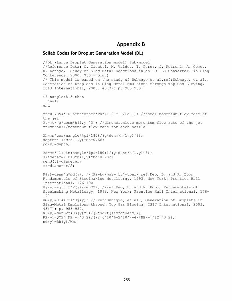
255

15 Appendix B

Scilab Codes for Droplet Generation Model (DL)

//DL (Lance Droplet Generation model) Sub-model




// This model is based on the study of Subagyo et al.ref:Subagyo, et al.,

Generation of Droplets in Slag-Metal Emulsions through Top Gas Blowing,

ISIJ International, 2003. 43(7): p. 983-989.

if nangle<8.5 then

nn=1;

end

mt=0.7854*10^5*nn*dth^2*Pa*(1.27*P0/Pa-1); //total momentum flow rate of

the jet

Mt=mt/(g*denm*h(1,y)^3); //dimensionless momentum flow rate of the jet

mn=mt/nn;//momentum flow rate for each nozzle

Mh=mn*cos(nangle*%pi/180)/(g*denm*h(1,y)^3);

depth=4.469*h(1,y)*Mh^0.66;

pd(y)=depth;

Md=mt*(1+sin(nangle*%pi/180))/(g*denm*h(1,y)^3);

diameter=2.813*h(1,y)*Md^0.282;

pend(y)=diameter;

rr=diameter/2;

P(y)=denm*g*pd(y); //(Pa=kg/ms2= 10^-5bar) ref:Deo, B. and R. Boom,

Fundamentals of Steelmaking Metallurgy, 1993, New York: Prentice Hall

International, 176-190

Uj(y)=sqrt(2*P(y)/denO2); //ref:Deo, B. and R. Boom, Fundamentals of

Steelmaking Metallurgy, 1993, New York: Prentice Hall International, 176-

190

UG(y)=0.44721*Uj(y); // ref:Subagyo, et al., Generation of Droplets in

Slag-Metal Emulsions through Top Gas Blowing, ISIJ International, 2003.

43(7): p. 983-989.

NB(y)=denO2*(UG(y)^2)/(2*sqrt(stm*g*denm));

RB(y)=QO2*(NB(y)^3.2)/((2.6*10^6+2*10^(-4)*NB(y)^12)^0.2);

nd(y)=RB(y)/Wm;

256

16 Appendix C

C.1 Scilab Codes for Flux Dissolution Model (FD)

//FD (Flux dissolution model) Sub-model




//This model uses mass transfer coefficient of CaO and MgO applying

equation from Clift et al. ref: R. Clift, J. R. Grace and M. E. Weber:

Bubbles, Drops and Particles, Academic Press, New York, (1978), p.297

//The height of the slag is found from the relationship given for foamed

slag. ref: Fruehan, R.J. and S. Jung, Foaming Characteristics of BOF

Slags, ISIJ International, 2000, 40(4): p. 348-355.

//The weight percent of saturated MgO for OS slags is taken from phase

diagram ref:E. T. Turkdogan: Fundamentals of Steelmaking, The Institute

of Materials, London. (1996), p. 150.

//CaO saturation level is obtained from CaO-SiO2-FeO quasiternary phase

diagram. ref: Slag Atlas, 1995, pp. 126. This means that this calculation

includes the formation of 2CaO.SiO2

//Calculations are based on the previous composition of slag.

//Diffusivities of CaO and MgO are not constant and related to slag

viscosity and temperature

//Mass transfer coefficient is calculated for laminar flow for dolomite

and lime dissolution

WCaOsat=list([42.14;44.2;46.4;47.14;48.92;50;50.71;52.86;53.57;53;52.85;5

2.14;51.78;51.42;52.5;53]); //the weight percent of saturated CaO (mass

%)

MgOref=18;

nes=10; //constant to modify settling velocity

dt=1;

MLime($+1)=MLime($)+Mflx(1,y+1); //the amount of CaO charged to the

process for the first two minutes (t)

MDolomite($+1)=MDolomite($)+Mflx(2,y+1);//the amount of MgO charged to

the process for the first two minutes (t)

WMgOsat=MgOref+(0.0175*(Ts($)-1873)); //the weight percent of saturated

MgO (mass %)

DcoeffMgO=AD*Ts($)/viss($); //diffusivity coefficient of MgO (m2/min)

DcoeffCaO=AL*Ts($)/viss($); //diffusivity coefficient of CaO (m2/min)

ScMgO=(viss($)/dens($))/(DcoeffMgO); //Schmitt number for dolomite

spheres

ScCaO=(viss($)/dens($))/(DcoeffCaO); //Schmitt number for lime spheres

u=y-1;

if nLime(y)>0 then

rLime(y,u)=r0Lime; end

if nDolomite(y)>0 then

rDolomite(y,u)=r0Dolomite; end

p=0;

ot=0;

m = list();

257

o = list();

for k=2:1:y

if rLime(k,u)>0 then

uCaO=abs(3600*(dens($)-

dLime)*g/9/(viss($)^0.5)/(dens($)^0.5))^(2/3)*2*rLime(k,u);

ReCaO=uCaO*2*rLime(k,u)*dens($)/viss($); //Reynolds number for

lime particles

ShCaO=1+0.724*nes^(0.48)*ReCaO^(0.48)*ScCaO^(1/3); //Sherwood

number for lime particles

kLime=ShCaO*DcoeffCaO/(2*rLime(k,u)); //mass transfer

coefficient for lime dissolution (m/min)

rLime(k,y)=rLime(k,u)-dens($)*kLime*dt*(WCaOsat(1)(x)-

Wox(x,3))/(dLime*100);

else

rLime(k,y)=0;

end

if rDolomite(k,u)>0 then

uMgO=abs(3600*(dens($)-

dDolomite)*g/9/(viss($)^0.5)/(dens($)^0.5))^(2/3)*2*rDolomite(k,u);

//velocity of dolomite particles (m/min)

ReMgO=uMgO*2*rDolomite(k,u)*dens($)/viss($); //Reynolds number

for dolomite particles

ShMgO=1+0.724*nes^(0.48)*ReMgO^(0.48)*ScMgO^(1/3); //Sherwood

number for dolomite particles

kDolomite=ShMgO*DcoeffMgO/(2*rDolomite(k,u)); //mass transfer

coefficient for dolomite dissolution (m/min) ref:mass transfer

coefficient for dolomite dissolution (m/min)

if Wox(x,1)<20 then

rDolomite(k,y)=rDolomite(k,u)-

(1+(MaO+MaMg)/(MaO+MaCa))*dens($)*kDolomite*dt*(WCaOsat(1)(x)-

Wox(x,3))/(dDolomite*100);

else

rDolomite(k,y)=rDolomite(k,u)-

(1+(MaO+MaCa)/(MaO+MaMg))*dens($)*kDolomite*dt*(WMgOsat-

Wox(x,4))/(dDolomite*100);

end

else

rDolomite(k,y)=0;

end

if rLime(k,y)==0

o($+1)=0;

UDLime(k,y)=UDLime(k,u);

ot=ot+1;

elseif rLime(k,y)< 0

o($+1)=UDLime(k,u);

UDLime(k,y)=0;

ot=ot+1;

elseif rLime(k,y)> 0

o($+1)=UDLime(k,u)-4/3*%pi*rLime(k,y)^3*dLime*10^(-3)*nLime(k);

UDLime(k,y)=4/3*%pi*rLime(k,y)^3*dLime*10^(-3)*nLime(k);

ot=ot+1;

end

if rDolomite(k,y)==0

m($+1)=0;

258

UDDolomite(k,y)=UDDolomite(k,u);

p=p+1;

elseif rDolomite(k,y)< 0

m($+1)=UDDolomite(k,u);

UDDolomite(k,y)=0;

p=p+1;

elseif rDolomite(k,y)> 0

m($+1)=UDDolomite(k,u)-4/3*%pi*rDolomite(k,y)^3*dDolomite*10^(-

3)*nDolomite(k);

UDDolomite(k,y)=4/3*%pi*rDolomite(k,y)^3*dDolomite*10^(-

3)*nDolomite(k);

p=p+1;

end

z=0;

op=0;

for t=1:1:ot

z=o(t)+z; end

for t=1:1:p

op=m(t)+op; end

end

C.2 Estimation of physical properties of slag

Part 1. Model for estimating the density of multicomponent slag

Model for density of slag has been widely used, which is given in Eq. (C.1). The recommended

values for the molar volume of slag constitutes are given in Table C.1.394)

s

FeOFeOMnOMnOMgOMgOCaOCaOSiOSiO

sV

xMxMxMxMxM22

++++=ρ (C.1)

FeOFeOMnOMnOMgOMgOCaOCaOSiOSiOs VxVxVxVxVxV22

++++= (C.2)

where M is molar weight (g/mole), X is mole fraction and Vs is partial molar volume of the slag

constitutes.

Table C.1. Recommended values for partial molar volume of slag constitutes at 1500 °C394)

Part 2. Model for estimating the viscosity of multicomponent slag

It has been known that viscosity of melt is sensitive to its ionic or molecular structure so the

changes in composition of slag and temperature profile of the slag should be included. The model

259

of Urbain et al.395) is considered in this calculation. Based on this model, slag constitutes are

divided into three groups for metallurgical slags:

1. Glass formers, 522 OPSiOG xxx +=

2. modifiers, 2222232 ZrOTiOCaFOKONaOFeFeOMnOMgOCaOM x2x2x3xxx5.1xxxxx +++++++++=

3. amphoterics, 322 OBOAlA xxx +=

Normalized values *

Gx , *

Mx and *

Ax are obtained by dividing the mole fractions, Gx , Mx and Ax

by the term (2225.1 ZrOTiOCaFFeO xxxx5.01 ++++ ). Parameter B can be found using

3*

G3

2*

G2

*

G10 )x(B)x(BxBBB +++= (C.3)

α is )xx/(x *

A

*

M

*

M + and B values can be found from Table C.2. Parameter A can be found by Eq.

(A.6) and viscosity of slag (in poise) can then be determined by using Eq. (C.5).

6725.11B2693.0Aln +=− (C.4)

)T/B10exp(AT 3

s =µ (C.5)

Table C.2. B parameters for calculating the viscosity of slag395)

C.3 Scilab Codes for Physical Properties of Slag

//Slag Properties

//The viscosity of slag is varied as a function of composition of slag

and temperature based on Urbain et al model. ref:Slag atlas pp. 353

//Based on Urbain et al model, xG=xSiO2+P2O5=mole farction for glass

formers in slag

//xM=xCaO+xMnO+xMgO+xFeO+1.5xFe2O3+3xCaF2=mole fraction of modifiers in

slag

//xAmphoterics=xAl2O3+xB2O3

B0=13.8+39.9355-44.049; //parameter to calculate B parameter for

viscosity of slag ref:Slag Atlas pp 350

B1=30.481-117.1505+139.9978;//parameter to calculate B parameter for


B2=-40.9429+234.0486-300.04;//parameter to calculate B parameter for


B3=60.7619-153.9276+211.1616;//parameter to calculate B parameter for


260

//calculation of slag properties for tb=2. The slag composition is not

known for tb=1. So the composition of slag at tb=2 is used for

calculation of slag properties at 2. min

//It is assumed that partial volume of metal oxides, viscosity of slag

and density of slag at time=t is the function of slag temperature at

time=t

//mole fraction of metal oxides in slag

xSiO2=(Wox(x,2)/(Mai(1,2)+2*MaO))/(Wox(x,2)/(Mai(1,2)+2*MaO)+Wox(x,1)/(Ma

Fe+MaO)+Wox(x,3)/(MaCa+MaO)+Wox(x,4)/(MaMg+MaO)+Wox(x,5)/(Mai(1,3)+MaO));

xCaO=(Wox(x,3)/(MaCa+MaO))/(Wox(x,2)/(Mai(1,2)+2*MaO)+Wox(x,1)/(MaFe+MaO)

+Wox(x,3)/(MaCa+MaO)+Wox(x,4)/(MaMg+MaO)+Wox(x,5)/(Mai(1,3)+MaO));

xMgO=(Wox(x,4)/(MaMg+MaO))/(Wox(x,2)/(Mai(1,2)+2*MaO)+Wox(x,1)/(MaFe+MaO)


xFeO=(Wox(x,1)/(MaFe+MaO))/(Wox(x,2)/(Mai(1,2)+2*MaO)+Wox(x,1)/(MaFe+MaO)


xMnO=(Wox(x,5)/(Mai(1,3)+MaO))/(Wox(x,2)/(Mai(1,2)+2*MaO)+Wox(x,1)/(MaFe+

MaO)+Wox(x,3)/(MaCa+MaO)+Wox(x,4)/(MaMg+MaO)+Wox(x,5)/(Mai(1,3)+MaO));

//density calculation

pVCaO=20.7+0.01*Ts($-1)*xCaO; //cm3/mol recommended values for

partial volume of CaO at 1500C ref:Slag Atlas pp346

pVMgO=16.1+0.01*Ts($-1)*xMgO; //cm3/mol recommended values for

partial volume of MgO at 1500C ref:Slag Atlas pp346

pVFeO=15.8+0.01*Ts($-1)*xFeO; //cm3/mol recommended values for

partial volume of FeO at 1500C ref:Slag Atlas pp346

pVMnO=15.6+0.01*Ts($-1)*xMnO; //cm3/mol recommended values for

partial volume of MnO at 1500C ref:Slag Atlas pp346

pVSiO2=19.55+7.966*xSiO2+0.01*Ts($-1)*xSiO2; //cm3/mol recommended

values for partial volume of SiO2 at 1500C ref:Slag Atlas pp346

VmSl=xCaO*pVCaO+xMgO*pVMgO+xFeO*pVFeO+xMnO*pVMnO+xSiO2*pVSiO2;

//molar volume of slag (cm3/mol) ref:Slag Atlas pp345

dens($+1)=1000*(xCaO*(MaCa+MaO)+xMgO*(MaMg+MaO)+xFeO*(MaFe+MaO)+xMnO*(Mai

(1,3)+MaO)+xSiO2*(Mai(1,2)+2*MaO))/VmSl; //the density of slag (kg/m3)

ref:Slag Atlas pp345fG=VG/(VG+VSl+VM)

//viscosity calculation

xG=xSiO2 ; xM=xCaO+xMgO+xFeO+xMnO;

B=B0+B1*xG+B2*xG^2+B3*xG^3; A=exp(-(0.2693*B+11.6725));

vis($+1)=A*Ts($-1)*exp(1000*B/Ts($-1))*6; //viscosity of slag based

on Urbain et al model (kg/mmin)ref:Slag Atlas pp380

viss($+1)=vis($);

261

17 Appendix D

Scilab Codes for Scrap Melting Model (SD)

//SD (Scrap dissolution model) Sub-model




//The calculation of scrap temperature can be obtained by error function

based on the equation 9.88 in Transport Phenomena by Geiger and Poirier

pp 307.

// Time step is selected as 5 seconds

time=sctime;

dt=10;

Cint($+1)=C($);

if Cint($)>4.27

Ti($+1)=1425;

else

Ti($+1)=1809-90*Cint($);

end

thold=thic($); tha=thic($);

TScold=TSc($); TSca=TSc($);

Tiold=Ti($); Tia=Ti($);

Told=T($); Ta=T($);

Tmold=Tb(x); Tma=Tb(x);

Lold=L($); La=L($);

xold=xsc($); xa=xsc($);

WScold=WSc($); WSca=WSc($);

Cpsc=(17.49+24.769*10^(-3)*Ta)*1000/56; //specific heat of scrap

(J/molK)ref:Sethi, G., et al. Theoretical Aspects of Scrap Dissolution in

Oxygen Steelmaking Converters. in AISTech 2004 Proceedings. 2004: The

Association of Iron & Steel Technology.

conducSc=densc*Cpsc*alfa; //thermal conductivity of scrap

(W/mK)ref:Sethi, G., et al. Theoretical Aspects of Scrap Dissolution in



hcoeff=17000;

n=1;

a=(1-cos(n*%pi))*(Tsci-Tiold)/(n*%pi/2); l=list(a);

m =l($)*(n*%pi/thold)*exp(-alfa*(conducSc)^2*time); k=list(m);

for n=2:1:3

a=(1-cos(n*%pi))*(Tsci-Tiold)/(n*%pi/2); l($+1)=a;

m=l($)*(n*%pi/thold)*exp(-alfa*(conducSc)^2*time); k($+1)=m;

end;

v=0; for r=1:1:3, v=k(r)+v; end

HF1=hcoeff*(Tmold-Tiold);

HF3=conducSc*v;

if msc($) < 0 then

if abs(HF3) > abs(HF1)

Ta=(Tiold+TScold)/2;

Bi=hcoeff*Li/conducSc;

262

Fo=alfa*time/Li^2;

Z=1-(erfc((1-

xold/Li)/(2*sqrt(Fo)))+erfc((1+xold/Li)/(2*sqrt(Fo))))+exp(Bi*(1-

xold/Li)+(Bi^2)*Fo)*erfc(Bi*sqrt(Fo)+(1-

xold/Li)/(2*sqrt(Fo)))+exp(Bi*(1+xold/Li)+(Bi^2)*Fo)*erfc(Bi*sqrt(Fo)+(1+

xold/Li)/(2*sqrt(Fo)));

Tsca=Z*(Tsci-Tmold)+Tmold;

Tscold=Tsca;

Cpsc=(17.49+24.769*10^(-3)*Ta)*1000/56; //specific heat of scrap

(J/molK)ref:Sethi, G., et al. Theoretical Aspects of Scrap Dissolution in



conducSc=densc*Cpsc*alfa; //thermal conductivity of scrap

(W/mK)ref:Sethi, G., et al. Theoretical Aspects of Scrap Dissolution in



n=1;



for n=2:1:3



end;

v=0; for r=1:1:3, v=k(r)+v; end

deltaH=deltah+Cpm*(Tmold-Tiold);


HF3=conducSc*v;

HF2=HF1+HF3;

rate=(HF1+HF3)/(-densc*deltaH);

deltaL=rate*dt;

xa=xold-deltaL/2;

tha=thold+deltaL;

La=tha/2;

msc($+1)=deltaL*densc*area*nsc;//the amount of scrap melted (kg)

WSca=WScold+msc($);

WSc($+1)=WSca;

TSc($+1)=Tsca;

thic($+1)=tha;

L($+1)=tha/2;

xsc($+1)=xa;

Mrate($+1)=rate;

Ti($+1)=Tia;

T($+1)=Ta;

elseif tha > thicknessSc


Fo=alfa*time/Li^2;

Z=1-(erfc((1-






263

Tscold=Tsca;


Cpsc=(17.49+24.769*10^(-3)*Ta)*1000/56;

conducSc=densc*Cpsc*alfa;

Tmold=Tb(y);

n=1;



for n=2:1:3



end;

v=0; for r=1:1:3, v=k(r)+v; end



HF3=conducSc*v;

HF2=HF1+HF3;


deltaL=rate*dt;

xa=xold-deltaL/2;

tha=thold+deltaL;

La=tha/2;

msc($+1)=deltaL*densc*area*nsc;

WSca=WScold+msc($);

WSc($+1)=WSca;

TSc($+1)=Tsca;

thic($+1)=tha;

L($+1)=tha/2;

xsc($+1)=xa;

Mrate($+1)=rate;

Ti($+1)=Tia;

T($+1)=Ta;

elseif tha > 0


Fo=alfa*time/Li^2;

Z=1-(erfc((1-






Tscold=Tsca;


Cpsc=(17.49+24.769*10^(-3)*Ta)*1000/56;

conducSc=densc*Cpsc*alfa;

n=1;



for n=2:1:3



end;

264

v=0; for r=1:1:3, v=k(r)+v; end



HF3=conducSc*v;

HF2=HF1+HF3;


deltaL=rate*dt;

xa=xold-deltaL/2;

tha=thold+deltaL;

La=tha/2;

msc($+1)=deltaL*densc*area*nsc;

WSca=WScold+msc($);

WSc($+1)=WSca;

TSc($+1)=Tsca;

thic($+1)=tha;

L($+1)=tha/2;

xsc($+1)=xa;

Mrate($+1)=rate;

Ti($+1)=Tia;

T($+1)=Ta;

end

end

sctime=sctime+dt;

265

18 Appendix E

Scilab Codes for Droplet Residence Model (RD)

//RD (Droplet Residence Model) Sub-model

//using ballistic motion principle



// Initialisation

//Dimension

dt=0.0001;

time=0;

initime=0;

timestep=0.01;

kstep=0;

kstep=timestep/dt;

ntime=9999;

uz=(1:ntime);

ur=(1:ntime);

lz=(1:ntime);

lr=(1:ntime);

tim=(1:ntime);

tim(1)=initime;

Ce=(1:ntime);

Diam=(1:ntime);

//Calculate parameters

//General

x=x;

y=y;

Wm=Wm0;

dend0=7000;

dend=dend0;

deng=1.25*273/Ts($);

denS=dens($);

visS=viss($)/60;

Tslag=Ts($);

densg=deng*fig($)+denS*(1-fig($));

vissg=2/3*visS*(densg-deng)/(1-fig($)^(1/3))/(denS-deng);

denS=densg;

visS=vissg;

cons=DiffC*1873/vism;

lz(1)=0;

lr(1)=0;

lza=0;

lra=0;

lzaold=0;

lraold=0;

266

Dd=Dd0;

fCd(y)=1873*fCd(8)/Ts($);

Ceq(y)=1/fCd(y)/gFeO(y)/xFeO/Kc(y);

Ce(1)=Cc;

FeO=Wox(x,1);

Cceq=Ceq(y);

EKG=NB(y)*QO2*3600*sqrt(stm*g*denm); //kinetic energy of blowing gas

(kgm2/min3)

EKD=EKG*0.00143*NB(y)^(0.7); // kinetic energy absorbed by the

droplets (kgm2/min3)

vec=sqrt(2*EKD/RB(y))/60; //initial velocity of droplet (m/s)

inivel($+1)=vec;

angle=60;

theta=angle*2*%pi/360;

ur(1)=vec*sin(theta);

uz(1)=vec*cos(theta);

uraold=ur(1);

uzaold=uz(1);

ura=ur(1);

uza=uz(1);

k=0;

ip=1;

istep=1;

while lza>=0

k=k+1;

ip=ip+1;

uzaold=uza;

uraold=ura;

lzaold=lza;

lraold=lra;

K0=(denS-dend)*9.81/(denS/2+dend);

Rer=denS*Dd/visS*abs(uraold);

if uraold <= 1.e-10

uraold=0;

Rer=1.e-10;

end

Cdr=24/Rer;

if ((Rer >= 1) & (Rer < 1000))

Cdr=18.5*Rer^(-0.6);

elseif Rer >= 1000

Cdr=0.44;

end

Rez=denS*Dd/visS*abs(uzaold);

Cdz=24/Rez;

if ((Rez >= 1) & (Rez < 1000))

Cdz=18.5*Rez^(-0.6);

elseif Rez >= 1000

Cdz=0.44;

end

Kr=-3*Cdr/2/(1+2*dend/denS)/Dd;

Kz=-3*Cdz/2/(1+2*dend/denS)/Dd;

if uzaold < 0

Kz=3*Cdz/2/(1+2*dend/denS)/Dd;

end

if uraold <= 1.e-10

Kr=0;

267

end

ura=uraold+dt*Kr*uraold*uraold;

uza=uzaold+dt*K0+dt*Kz*uzaold*uzaold;

lza=lzaold+0.5*dt*(uza+uzaold);

lra=lraold+0.5*dt*(ura+uraold);

if lza >= slagh

lza=slagh;

end

time=time+dt;

// Chemical reactions

//1. Decarburization

Vel=sqrt(ura*ura+uza*uza);

Ccold=Cc;

if FeO > 20 then

rccr=2.86e-4*20;

else

rccr=2.86e-4*FeO;

end

Area=%pi*Dd*Dd;

Volum=%pi*Dd*Dd*Dd/6;

DiffC=cons*vism/Tslag;

kk=2*sqrt(DiffC*Vel/%pi/Dd);

ka=kk*Area/Volum;

Cc=Cceq+(Ccold-Cceq)*exp(-(ka*dt));

//End of decarburization

//2. Calculation of density change

rc=(Ccold-Cc)/dt;

if rc > rccr

dend=dend0*rccr/rc;

end

if rc <= rccr

dend=dend0;

end

Wm=Wm-Wm*(Ccold-Cc)/100;

Volum=Wm/dend;

Dd=(6*Volum/%pi)^(1/3);

//End of Calculation of density change

if abs(k-kstep) < dt

istep=istep+1;

tim(istep)=time;

ur(istep)=ura;

uz(istep)=uza;

lr(istep)=lra;

lz(istep)=lza;

Ce(istep)=Cc;

Diam(istep)=Dd;

k=0;

end

end

TotalSteps=ip-1;

ResiTime=time;

Cc;

268

Scilab Codes for Equilibrium Calculations

//Changes in equilibrium composition in metal bath and slag




//reaction within metal droplet in slag; (FeO)+[C]=Fe+(CO)g

//Activity coeffient of metal oxides in oxygen steelmaking slag are found

on the basis of regular solution model proposed by Banya.

// Initialisation

aFe=1:

fCss=0.57: //activity coefficient of carbon at standard state

ref:Steelmaking data source, Revised by The Japan Society for the

promotion of science, The 19th Committee on steelmaking 1988)

fSiss=0.0013: //activity coefficient of silicon at standard state



fOss=0.0109: //activity coefficient of oxygen at standard state



fMnss=1.3: //activity coefficient of manganese at standard state



//calculation of activity coefficient of carbon in metal droplet as a

function of temperature with time. The carbon content of droplet is used

as a data in the calculations.

//Intcoeff=['coef','Si','C','Mn','O'] =interaction coefficients of

elements in liquid iron at 1600C

Intcoeff=[

0.11 0.207 0.002 -0.23

0.09 0.154 -0.012 -0.34

0 -0.07 0 -0.083

-0.131 -0.45 -0.021 -0.327

]:

//calculation of activity coefficient of FeO in slag as a function of

temperature with time

//Intenergy=['coef','Fe+2','Fe+3','Mn2+','Ca2+','Mg2+','Si4+']

=Interaction energy between cations of major components in steelmaking

slag, aij

Intenergy=[

0 -18660 7110 -31380 33470 -41840;

-18660 0 -56480 -95810 -2930 32640;

7110 -56480 0 -92050 61920 -75310;

-31380 -95810 -92050 0 -100420 -133890;

33470 -2930 61920 -100420 0 -66940;

-41840 32640 -75310 -133890 -66940 0];

//calculation of equilibrium constant

hcC=10^(0.154*2); //henrian acitivity coefficient of carbon at

droplet in slag at 1600C (It is assumed that the carbon concentration is

2 mass % in the droplet at 1600C)

269

rcC=hcC*fCss; //raultian activity coefficient of carbon at droplet in

slag at 1600C

Kc($+1)=10^(5.096-5730/Ts($));

KFe(y)=10^(-6372/Tb($)+2.73);

gFeO($+1)=exp((Intenergy(1,6)*xSiO2^2+Intenergy(1,4)*xCaO^2+Intenergy(1,5

)*xMgO^2+Intenergy(1,3)*xMnO^2+(Intenergy(1,6)+Intenergy(1,4)-

Intenergy(6,4))*xSiO2*xCaO+(Intenergy(1,6)+Intenergy(1,5)-

Intenergy(6,5))*xSiO2*xMgO+(Intenergy(1,6)+Intenergy(1,3)-

Intenergy(6,3))*xSiO2*xMnO+(Intenergy(1,4)+Intenergy(1,5)-

Intenergy(4,5))*xCaO*xMgO+(Intenergy(1,4)+Intenergy(1,3)-

Intenergy(4,3))*xCaO*xMnO+(Intenergy(1,5)+Intenergy(1,3)-

Intenergy(5,3))*xMgO*xMnO)/8.314/Ts($-1));

aFeO(y)=gFeO($)*xFeO;

270

19 Appendix F

Scilab Codes for Decarburization Reaction in the Emulsion Model (DCE)

//DCE (Decarburization in Emulsion) Sub-model

//using bulk carbon content

Crange(a,a)=C($);

DiamRange(a,a)=Dd0;

Cc=C($);


sec\RD.sci', [,0]);

y=y:

tr=ResiTime/60;

DrTime(a,a)=tr;

model(a,11)=tr;

model(a,4)=Cc;

iz=a;

u=iz+1;

p=iz-1;

ot=0;

op=0;

om =list();

m= list();

n= list();

o= list();

od= list();

mn= list();

dt=1/i:

if tr < dt

Crange(a,b)=Cc;

DiamRange(a,b)=Dd;

Veloz(a,b)=uza;

Velor(a,b)=ura;

Traz(a,b)=lza;

Trar(a,b)=lra;

end

if tr > dt

for z=10:10:ResiTime

Crange(a,b)=Ce(z*100);

DiamRange(a,b)=Diam(z*100);

Veloz(a,b)=uz(z*100);

Velor(a,b)=ur(z*100);

Traz(a,b)=lz(z*100);

Trar(a,b)=lr(z*100);

b=b+1:

end

Crange(a,b)=Cc;

DiamRange(a,b)=Dd;

Veloz(a,b)=uza;

Velor(a,b)=ura;

Traz(a,b)=lza;

Trar(a,b)=lra;

271

end

for k=1:1:iz

if k==iz then

DrTime(k,iz)=DrTime(k,k);

else

DrTime(k,iz)=DrTime(k,p)-dt;

end

if DrTime(k,iz) > 0

if DrTime(k,iz) <= dt

RD(k,iz)=RBi(k);

m($+1)=RBi(k)*DrTime(k,iz);

if DrTime(k,iz)<0.001

n($+1)=0;

else

n($+1)=Wm*ndi(k)*abs(Crange(k,iz)-

Crange(k,u))/100/DrTime(k,iz);

end

od($+1)=RBi(k)*dt-Wm*ndi(k)*abs(Crange(k,k)-

Crange(k,u))/100;

om($+1)=ndi(k)*(%pi*DiamRange(k,u)*DiamRange(k,u)*DiamRange(k,u)/6-

Volum0):

ot=ot+1;

else

RD(k,iz)=0;

m($+1)=RBi(k)*dt;

n($+1)=Wm*ndi(k)*abs(Crange(k,iz)-Crange(k,u))/100/dt;

od($+1)=0;

om($+1)=ndi(k)*(%pi*DiamRange(k,u)*DiamRange(k,u)*DiamRange(k,u)/6-

Volum0);

ot=ot+1;

end

end

if (DrTime(k,iz) < 0) & (DrTime(k,iz)>-dt)

mn($+1)=Wm*ndi(k)*abs(Crange(k,k)-Crange(k,u))/100;

op=op+1;

else

mn($+1)=0;

op=op+1;

end

oz=0;

w=0;

on=0;

omm=0;

mnn=0;

for t=1:1:ot

oz=m(t)+oz;

w=n(t)+w;

on=od(t)+on;

omm=om(t)+omm; end

for t=1:1:op

mnn=mnn+mn(t);

end

272

end

Vd($+1)=oz;

Vb($+1)=on;

Wc($+1)=w;

Wcc($+1)=mnn;

Vgg($+1)=omm;

model(a,7)=oz;

model(a,8)=on;

model(a,12)=w;

model(a,13)=mnn;

model(iz,59)=omm;

273

20 Appendix G

G.1 Scilab Codes for Decarburization Reaction in the Impact Zone (DCI)

//DCI (Decarburization Reaction in Impact Zone Model) Sub-model




cons=DiffC*1873/vism;


Vt=QNAr*Tb(y)/(293*1.5)/60; //total gas flow rate at bath conditions

(m3/s)

//calculation of jet penetration characteristics

D=h(1,y)/dth;

Ue=500; //velocity of gas at nozzle exit (m/s)

denO2e=2.33; //density of oxygen at nozzle exit (kg/m3)

Momentum=%pi*denO2e*Ue^2*de^2/4;

//calculation of interfacial area

hstep=0.001;

rold=0;

ra=0;

dcold=0;

dca=0;

hlimit=(-depth);

hcold=hlimit;

hca=hlimit;

istep=0;

Area=0;

m = list();

ra=0;

while hca <= -0.001

hca=hcold+hstep;

ra=ra+0.008;

if ra > rr then

break

end

Area=Area+2*%pi*rold*(ra-rold)*sqrt(1+((hca-hcold)/(ra-rold))^2);

hcold=hca;

dcold=dca;

rold=ra;

m($+1)=ra;

istep=istep+1;

end

A=Area*6;

oz=0;

for t=1:1:istep

oz=m(t)+oz; end

r0=oz/istep;

//calculation of CO2 gas velocity

274

U=UG(y); //velocity of gas (m/s)

//calculation of mass transfer coefficient for CO2

ScCO2=visCO2/denCO2/DiffCO2;

ReCO2=U*r0/(visCO2/denCO2);

ShCO2=0.026*ReCO2^1.06*ScCO2^0.33*D^(-0.09);

kmCO2=ShCO2*DiffCO2/r0/R/TfCO2($); //(mole/m2.s.atm)

//calculation of chemical reaction constant for CO2

KS=10^(3600/Timpact($)+0.57);//(1/mass %)

kf=10^(-5080/Timpact($)-0.21);//(mole/cm2.s.atm)

kr=10^(-5600/Timpact($)-1.75);//(mole/cm2.s.atm)

kt=10^4*(kf/(1+KS*Sulphur)+kr);//(mole/m2.s.atm)

//calculation of overall rate constant for CO2

kg=kmCO2*kt/(kmCO2+kt); //(mole/m2.s.atm)

//decarburization rate of reaction (C+CO2=2CO)

RateCO2($+1)=12*60/1000*A*kg*PbCO2; //kg/min

//calculation of mass transfer coefficient for O2

ScO2=visO2/denO2/DiffO2;

ReO2=U*r0/(visO2/denO2);

ShO2=0.026*ReO2^1.06*ScO2^0.33*D^(-0.09);

kmO2=ShO2*DiffO2/r0/R/TfO2($); //(mole/m2.s.atm)

//decarburization rate of reaction (CO+1/2O2=CO2)

RateO2($+1)=24*60/1000*A*kmO2*log(1+PbO2); //kg/min

//calculation of mass transfer coefficient in liquid phase

DiffC=cons*vism/Tb(y);//diffusivity of carbon in metal (m2/s)

kkb=500*sqrt(DiffC*Vt/A);//(m/s)

RateDiff($+1)=kkb*A*denm*60/100*C($);//kg/min

TotalRate=RateCO2($)+RateO2($); //kg/min

Min=TotalRate-25;

Max=TotalRate+25;

if (RateDiff($)>Min) & (RateDiff($)<Max) then

Ccr=TotalRate/kkb/A/denm/60*100;

end

//calculation of rate

if C($)> 0.5

RateBath($+1)=RateCO2($)+RateO2($); //kg/min

else

RateBath($+1)=kkb*A*denm*60/100*C($);//kg/min

end

model(iz,14)=RateBath($);

model(iz,16)=Vt;

model(iz,17)=A;

model(iz,18)=r0;

model(iz,19)=visCO2;

model(iz,20)=denCO2;

model(iz,21)=DiffCO2 ;

275

model(iz,22)=ReCO2 ;

model(iz,23)=ScCO2;

model(iz,24)=ShCO2 ;

model(iz,25)=kmCO2;

model(iz,26)=kt ;

model(iz,27)=kg ;

model(iz,28)=PbCO2;

model(iz,29)=RateCO2($);

model(iz,30)=visO2;

model(iz,31)=denO2;

model(iz,32)=DiffO2 ;

model(iz,33)=ReO2 ;

model(iz,34)=ScO2 ;

model(iz,35)=ShO2 ;

model(iz,36)=kmO2;

model(iz,37)=PbO2;

model(iz,38)=RateO2($);

model(iz,39)=kkb ;

model(iz,40)=RateDiff($);

model(iz,41)=TotalRate;

model(iz,42)=Ccr;

G.2 Scilab Codes for Physical Properties of Slag


sec\global variables.sci', [,0])

// Initialisation

// Dimension

MaCO2=2*MaO+Mai(1,1);

MaO2=2*MaO;

dcO2=3.433;// collosion diameter of oxygen (A) ref:J. O. Hirschfelder, R.

B. Bird and E. L. Spotz: The Journal of Chemical Physics, 16(1948), 968.

dcCO=3.59;// collosion diameter of carbon monoxide (A) ref:J. O.

Hirschfelder, R. B. Bird and E. L. Spotz: The Journal of Chemical

Physics, 16(1948), 968.

dcCO2=3.996;// collosion diameter of carbon dioxide (A) ref:J. O.


Physics, 16(1948), 968.

EkO2=113.2; //potential diameter of carbon dioxide(K) ref:J. O.


Physics, 16(1948), 968.

EkCO=110.3; //potential diameter of carbon monoxide(K) ref:J. O.


Physics, 16(1948), 968.

EkCO2=190; //potential diameter of carbon dioxide(K) ref:J. O.


Physics, 16(1948), 968.

//calculation of density of gases

denO2=Pa*MaO2/R/TfO2($)*10^(-3); //kg/m3

denCO2=Pa*MaCO2/R/TfCO2($)*10^(-3); //kg/m3

//calculation of viscosity of gases

visconsCO2=1.147*(TfCO2($)/EkCO2)^(-0.145)+(TfCO2($)/EkCO2+0.5)^(-2);//

constant to calculate viscosity at 1600K ref:L. D. Cloutman: A database

276

of selected transport coefficients for combustion studies, Lawrence

Livermore National Laboratory, Livermore, California, (1993),15

visconsO2=1.147*(TfO2($)/EkO2)^(-0.145)+(TfO2($)/EkO2+0.5)^(-2);//

constant to calculate viscosity at 1600K ref:L. D. Cloutman: A database

of selected transport coefficients for combustion studies, Lawrence

Livermore National Laboratory, Livermore, California, (1993),15

visCO2=266.93*10^(-

7)*sqrt(MaCO2*TfCO2($))/visconsCO2/dcCO2^2*0.1;//viscosity of CO2

(kg/m.s) ref:R. I. L. Guthrie: Engineering in Process Metallurgy, Oxford

University Press Inc., New York, (1989), 43-45.

visO2=266.93*10^(-7)*sqrt(MaO2*TfO2($))/visconsO2/dcO2^2*0.1;//viscosity

of CO2 (kg/m.s) ref:R. I. L. Guthrie: Engineering in Process Metallurgy,

Oxford University Press Inc., New York, (1989), 43-45.

//calculation of diffusivity of gases

EkCO2CO=sqrt(EkCO2*EkCO);

diffconsCO2=(TfCO2($)/EkCO2CO)^(-0.145)+(TfCO2($)/EkCO2CO+0.5)^(-2);

dcCOCO2=0.5*(dcCO+dcCO2);

DiffCO2=0.0018583*sqrt(TfCO2($)^3*(MaCO2+MaCO)/MaCO2/MaCO)/Pa/dcCOCO2^2/d

iffconsCO2*10^(-4); //(m2/s) ref:D. R. Poirier and G. H. Geiger:

Transport Phenomena in Material Processing, The Minerals, Metals and

Materials of Society, Warrandale, Pennsylvania, (1994), 464.

EkO2CO=sqrt(EkO2*EkCO);

diffconsO2=(TfO2($)/EkO2CO)^(-0.145)+(TfO2($)/EkO2CO+0.5)^(-2);

dcCOO2=0.5*(dcCO+dcO2);

DiffO2=0.0018583*sqrt(TfO2($)^3*(MaO2+MaCO)/MaO2/MaCO)/Pa/dcCOO2^2/diffco

nsO2*10^(-4); //(m2/s) ref:D. R. Poirier and G. H. Geiger: Transport

Phenomena in Material Processing, The Minerals, Metals and Materials of

Society, Warrandale, Pennsylvania, (1994), 464.