mathematical foundations of supervised learning - webhome · if yis continuous and the loss...
TRANSCRIPT

Mathematical Foundations ofSupervised Learning
(growing lecture notes)
Michael M. Wolf
June 6, 2018

Contents
Introduction 5
1 Learning Theory 71.1 Statistical framework . . . . . . . . . . . . . . . . . . . . . . . . . 71.2 Error decomposition . . . . . . . . . . . . . . . . . . . . . . . . . 91.3 PAC learning bounds . . . . . . . . . . . . . . . . . . . . . . . . . 151.4 No free lunch . . . . . . . . . . . . . . . . . . . . . . . . . . . . . 181.5 Growth function . . . . . . . . . . . . . . . . . . . . . . . . . . . 191.6 VC-dimension . . . . . . . . . . . . . . . . . . . . . . . . . . . . . 221.7 Fundamental theorem of binary classification . . . . . . . . . . . 291.8 Rademacher complexity . . . . . . . . . . . . . . . . . . . . . . . 311.9 Covering numbers . . . . . . . . . . . . . . . . . . . . . . . . . . 371.10 Pseudo and fat-shattering dimension . . . . . . . . . . . . . . . . 461.11 Algorithmic stability . . . . . . . . . . . . . . . . . . . . . . . . . 481.12 Relative entropy bounds . . . . . . . . . . . . . . . . . . . . . . . 531.13 Differential privacy . . . . . . . . . . . . . . . . . . . . . . . . . . 601.14 Ensemble methods . . . . . . . . . . . . . . . . . . . . . . . . . . 61
2 Neural networks 692.1 Information processing in the brain . . . . . . . . . . . . . . . . . 692.2 From Perceptrons to networks . . . . . . . . . . . . . . . . . . . . 712.3 Representation and approximation . . . . . . . . . . . . . . . . . 752.4 VC dimension of neural networks . . . . . . . . . . . . . . . . . . 852.5 Rademacher complexity of neural networks . . . . . . . . . . . . 892.6 Training neural networks . . . . . . . . . . . . . . . . . . . . . . . 912.7 Backpropagation . . . . . . . . . . . . . . . . . . . . . . . . . . . 932.8 Gradient descent and descendants . . . . . . . . . . . . . . . . . 942.9 (Un)reasonable effectiveness—optimization . . . . . . . . . . . . 1022.10 Deep neural nets . . . . . . . . . . . . . . . . . . . . . . . . . . . 1052.11 (Un)reasonable effectiveness—generalization . . . . . . . . . . . . 108
3 Support Vector Machines 1093.1 Linear maximal margin separators . . . . . . . . . . . . . . . . . 1093.2 Positive semidefinite kernels . . . . . . . . . . . . . . . . . . . . . 113
2

CONTENTS 3
3.3 Reproducing kernel Hilbert spaces . . . . . . . . . . . . . . . . . 1153.4 Universal and strictly positive kernels . . . . . . . . . . . . . . . 1173.5 Rademacher bounds . . . . . . . . . . . . . . . . . . . . . . . . . 120

4 CONTENTS

Introduction
These are (incomplete but hopefully growing) lecture notes of a course taught firstin summer 2016 at the department of mathematics at the Technical Universityof Munich. The course is meant to be a concise introduction to the mathematicalresults of the field.
What is machine learning? Machine learning is often considered as part ofthe field of artificial intelligence, which in turn may largely be regarded as asubfield of computer science. The aim of machine learning is to exploit datain order to devise complex models or algorithms in an automated way. Somachine learning is typically used whenever large amounts of data are availableand when one aims at a computer program that is (too) difficult to program‘directly’. Standard examples are programs that recognize faces, handwritingor speech, drive cars, recommend products, translate texts or play Go. Theseare hard to program from scratch so that one uses machine learning algorithmsthat produce such programs from large amounts of data.
Two main branches of the field are supervised learning and unsupervisedlearning. In supervised learning a learning algorithm is a device that receives‘labeled training data’ as input and outputs a program that predicts the labelfor unseen instances and thus generalizes beyond the training data. Examples ofsets of labeled data are emails that are labeled ‘spam’ or ‘no spam’ and medicalhistories that are labeled with the occurrence or absence of a certain disease.In these cases the learning algorithm’s output would be a spam filter and adiagnostic program, respectively.
In contrast, in unsupervised learning there is no additional label attachedto the data and the task is to identify patterns and/or model the data. Un-supervised learning is for instance used to compress information, to organizedata or to generate a model for it. In the following, we will exclusively dealwith supervised learning. Currently, supervised learning appears to be the bestdeveloped and economically most influential part of machine learning.
A first coarse classification of supervised learning algorithms is in terms ofthe chosen type of representation, which determines the basic structure of thegenerated programs. Common ones are:
• Decision trees
5
6 CONTENTS
• Nearest neighbors
• Neural networks
• Support vector machines and kernel methods
These types of representations, though quite different in nature, have two im-portant things in common: they enable optimization and they form universalhierarchies.
The fact that their structure enables optimization is crucial in order to iden-tify an instance (i.e., a program) that fits the data and presumably performswell regarding future predictions. This optimization is typically done in a greedymanner.
Forming a universal hierarchy means that the type of representation allowsfor more and more refined levels that, in principle, are capable of representingevery possibility or at least approximating every possibility to arbitrary accu-racy.
Only few such representation types are known and the above examples (to-gether with variations on the theme and combinations thereof) already seem tocover most of the visible universe.
We will focus on the last two of the mentioned types of representations,neural networks and support vector machines, which are arguably the mostsophisticated and most powerful ones. To begin with, however, we will have acloser look at the general statistical framework of supervised learning theory.
Chapter 1
Learning Theory
1.1 Statistical framework
In this section we set up the standard statistical framework for supervised learn-ing theory.
Input of the learning algorithm is the training data that is a finite sequence S =((x1, y1), . . . , (xn, yn)
)of pairs from X ×Y. yi is called the label corresponding
to xi.
Output of the learning algorithm is a function h : X → Y, called hypothesis,that aims at predicting y ∈ Y for arbitrary x ∈ X , especially for those notcontained in the training data. Formally, a learning algorithm can thus beseen as a map A : ∪n∈N(X × Y)n → YX . We will denote its range, i.e., theset of functions that can be output and thus be represented by the learningalgorithm, by F . From a computer science perspective the learning algorithmis an algorithm that, upon input of the training data S, outputs a computerprogram described by hS := A(S) ∈ F .
Probabilistic assumption. The pairs (xi, yi) are treated as values of randomvariables (Xi, Yi) that are identically and independently distributed accordingto some probability measure P over X × Y. We will throughout assume thatthe corresponding σ-algebra is a product of Borel σ-algebras w.r.t. the usualtopologies. All considered functions will be assumed to be Borel functions.Expectations w.r.t. P and Pn will be denoted by E and ES , respectively. Ifwe want to emphasize that, for instance, S is distributed according to Pn wewill use the more explicit notation ES∼Pn . Similarly, probabilities of eventsA and B w.r.t. P and Pn will be denoted by P[A] and PS [B], respectively.It is throughout assumed that P does not only govern the distribution of thetraining data, but also the one of future, yet unseen instances of data points.
Goal of the learning algorithm is to find a good hypothesis h w.r.t. a suitablychosen loss function L : Y × Y → R that measures how far h(x) is from the
7
8 CHAPTER 1. LEARNING THEORY
respective y. The smaller the average loss, called risk1 and given by
R(h) :=
∫
X×YL(y, h(x)
)dP (x, y), (1.1)
the better the hypothesis. The challenge is, that the probability measure P isunknown, only the training data S is given. Hence, the task of the learningalgorithm is to minimize the risk without being able to evaluate it directly.
Depending on whether Y is continuous or discrete one distinguishes twotypes of learning problems with different loss functions: regression problemsand classification problems2.
Regression
If Y is continuous and the loss function is, colloquial speaking, a distance mea-sure, the learning problem is called a regression problem. The most common lossfunction in the case Y = R is the quadratic loss L
(y, h(x)
)= |y−h(x)|2 leading
to the L2-risk also known as mean squared error R(h) = E[|Y − h(X)|2
]. For
many reasons this is a mathematically convenient choice. One of them is thatthe function that minimizes the risk can be handled:
Theorem 1.1: Regression function minimizes L2-risk
In the present context let h : X → Y = R be a Borel function and assumethat E
[Y 2]
and E[h(X)2
]are both finite. Define the regression function
as conditional expectation r(x) := E(Y |X = x). Then the L2-risk of hcan be written as
R(h) = E[|Y − r(X)|2
]+E
[|h(X)− r(X)|2
]. (1.2)
Note: The first term on the r.h.s. in Eq.(1.2) vanishes if there is a deterministicrelation between x and y, i.e., if P (y|x) ∈ 0, 1. In general, it can be regardedas unavoidable inaccuracy that is due to noise or due to the lack of informa-tion content in X about Y . The second term contains the dependence on hand is simply the squared L2-distance between h and the regression functionr. Minimizing the risk thus means minimizing the distance to the regressionfunction.
Proof. (sketch) Consider the real Hilbert space L2(X×Y, P ) with inner product〈ψ, φ〉 := E [ψφ]. h can be considered as an element of the closed subspace offunctions that only depend on x and are constant w.r.t. y. The function r also
1The risk also runs under the name out-of-sample error or generalization error.2Although this seems to be a reasonable working definition distinguishing regression from
classification, the difference between the two is not so sharp: discretized versions of continuousregression problems may still be called regression problems and, conversely, if the space Y isa space of probability distribution over the classes of interest, a problem may still be called aclassification problem.
1.2. ERROR DECOMPOSITION 9
represents an element of that subspace and since the conditional expectation3
is, by construction, the orthogonal projection into that subspace, we have 〈y −r, h− r〉 = 0. With this, Pythagoras’ identity yields the desired result
||y − h||2 = ||y − r||2 + ||h− r||2.
Classification
Classification deals with discrete Y, in which case a function from X to Y is alsocalled a classifier. The most common loss function in this scenario is the 0-1loss L(y, y′) = 1− δy,y′ so that the corresponding risk is nothing but the errorprobability R(h) = P [h(X) 6= Y ] = E
[1h(X)6=Y
]. We will at the beginning
often consider binary classification where Y = −1, 1. The error probabilityin binary classification is minimized by the Bayes classifier
b(x) := sgn(E [Y |X = x]
). (1.3)
1.2 Error decomposition
How can the learning algorithm attempt to minimize the risk R(h) over itsaccessible hypotheses h ∈ F without knowing the underlying distribution P?There are two helping hands. The first one is prior knowledge. This can for in-stance be hidden in the choice of F and the way the learning algorithm chooses ahypothesis from this class. Second, although R(h) cannot be evaluated directly,the average loss can be evaluated on the data S, which leads to the empiricalrisk, also called in-sample error
R(h) :=1
n
n∑
i=1
L(yi, h(xi)
). (1.4)
The approach of minimizing R is called empirical risk minimization (ERM). In
particular if |Y| < ∞, then there always exists a minimizer h ∈ F that attains
infh∈F R(h) = R(h) since the functions are only evaluated at a finite number ofpoints, which effectively restricts F to a finite space.
In general, ERM is a computationally hard task—an issue that we will dis-cuss in greater detail in the following chapters, where specific representationsare chosen. At this point, we will make the idealizing assumption that ERMcan be performed. Keeping in mind, however, that only in few cases an efficientalgorithm or a closed form solution for ERM is known, like in the followingexamples.
3If there is a probability density p(x, y), the conditional expectation is given by E(Y |X =x) =
∫Y y p(x, y)/p(x)dy, if the marginal p(x) is non-zero. For a general treatment of condi-
tional expectations see for instance [15], Chap.23.
10 CHAPTER 1. LEARNING THEORY
Example 1.1 (Linear regression). Let X × Y = Rd × R and F := h : X →Y | ∃v ∈ Rd : h(x) = 〈v, x〉 be the class of linear functions. The minimizer ofthe empirical risk (w.r.t. the quadratic loss)
R(v) :=1
n
n∑
i=1
(yi − 〈v, xi〉
)2, (1.5)
can be determined by realizing that the condition ∇R(v) = 0 can be rewrittenas linear equation Av = b, where A :=
∑i xix
Ti and b :=
∑i yixi. This is solved
by v = A−1b where the inverse is computed on range(A).
Example 1.2 (Polynomial regression). Let X × Y = R×R and F := h : R→R | ∃a ∈ Rm+1 : h(x) =
∑mk=0 akx
k be the set of polynomials of degree m.In order to find the ERM w.r.t. the quadratic loss, define ψ : R → Rm+1,ψ(x) := (1, x, x2, . . . , xm). Then the empirical risk can be written as
1
n
n∑
i=1
(yi −
m∑
k=0
akxki
)2
=1
n
n∑
i=1
(yi − 〈a, ψ(xi)〉
)2.
Hence, it is of the form in Eq.(1.5) and one can proceed exactly as in the caseof linear regression in Exp.1.1. Note that instead of using the monomial basisin the components of ψ, we could as well use a Fourier basis, Wavelets or otherbasis functions and again follow the same approach.
If n, the size of the training data set, is sufficiently large, one might hope thatR(h) is not too far from R(h) so that ERM would come close to minimizing therisk. The formalization and quantification of this hope is essentially the contentof the remaining part of this chapter.
To this end, and also for a better understanding of some of the main is-sues in supervised machine learning, it is useful to look at the following errordecompositions.
Let R∗ := infhR(h) be the so-called Bayes risk, where the infimum is takenover all measurable functions h : X → Y, and let RF := infh∈F R(h) quantifythe optimal performance of a learning algorithm with range F . Assume furtherthat a hypothesis h ∈ F minimizes the empirical, i.e., R(h) ≤ R(h) ∀h ∈ F .Then we can decompose the difference between the risk of a hypothesis h andthe optimal Bayes risk as
R(h)−R∗ =(R(h)−R(h)
)︸ ︷︷ ︸optimization error
+(R(h)−RF
)︸ ︷︷ ︸estimation error
+(RF −R∗
)︸ ︷︷ ︸
approximation error
. (1.6)
The approximation error does neither depend on the hypothesis nor on the data.It quantifies how well the hypothesis class F is suited for the problem underconsideration. The optimization error depends on how good the optimizationthet led to hypothesis h is relative to ideal empirical risk minimization. Theestimation error measures how well the empirical risk minimizer h performsrelative to a true risk minimizer in F . By the law of large numbers the estimation
1.2. ERROR DECOMPOSITION 11
error is expected to decrease with the size n of the training data set and to vanishasymptotically. The estimation error can be bounded by:
R(h)−RF = R
(h)− R
(h)
+ suph∈F
(R(h)−R(h)
)
≤ 2 suph∈F
∣∣∣R(h)−R(h)∣∣∣. (1.7)
Bounds on difference between the risk and the empirical risk (or, using syn-onyms, between the out-of-sample error and the in-sample error) are calledgeneralization bounds. They quantify how well the hypothesis generalizes fromthe observed data to unseen cases. Uniform generalization bounds, as desiredby Eq.(1.7), will be derived in the following sections.
Let us for the moment assume that the learning algorithm performs idealERM so that the optimization error vanishes. Then we are typically faced witha trade-off between the estimation error and the approximation error: whileaiming at a smaller approximation error suggests to take a richer hypothesisclass F , the data required to keep the estimation error under control unfortu-nately turns out to grow rapidly with the size or complexity of F (cf. followingsections). A closely related trade-off runs under the name bias-variance trade-off. It has its origin in a refinement of the decomposition in Thm.1.1 and isexemplified in Fig.1.1.
Theorem 1.2: Noise-bias-variance decomposition
In the setup of Thm.1.1 consider a fixed learning algorithm that outputsa hypothesis hS upon input of S ∈ (X × Y)n. Regard S as a randomvariable, distributed according to Pn and define h(x) := ES [hS(x)] theexpected prediction for a fixed x. If the expected risk ES [R(hS)] is finite,then it is equal to
E[|Y − r(X)|2
]︸ ︷︷ ︸
noise
+E[|h(X)− r(X)|2
]︸ ︷︷ ︸
bias2
+E[ES
[|hS(X)− h(X)|2
]]︸ ︷︷ ︸
variance
(1.8)
Proof. We take the expectation ES of Eq.(1.2) when applied to hS and observethat the first term on the r.h.s. is independent of S. For the second term weobtain
ES
[E[|hS(X)− r(X)|2
]]= E
[ES
[|hS(X)− h(X) + h(X)− r(X)|2
]]
= E[|h(X)− r(X)|2
]
+ E[ES
[|hS(X)− h(X)|2
]]
+ 2E[ES
[(hS(X)− h(X)
)(h(X)− r(X)
)]].
The term in the last line vanishes since(h(X)− r(X)
)is independent of S and
ES
[(hS(X)− h(X)
)]= 0.

12 CHAPTER 1. LEARNING THEORY
Figure 1.1: Bias-variance trade-off in polynomial regression: two samples (redand blue points) are drawn from the same noisy version of a quadratic function(gray). If we fit high degree polynomials (top image), there is a large variancefrom sample to sample, but a small bias in the sense that the average curveasymptotically matches the underlying distribution well. If affine functions areused instead (bottom image), the variance is reduced at the cost of a large bias.
As can bee seen in the example of polynomial regression in Fig.1.1, if we increasethe size of F , then the squared bias is likely to decrease while the variance willtypically increase (while the noise is unaffected).
There is a third incarnation of the phenomenon behind a dominating varianceor estimation error that is called overfitting. All together these are consequencesof choosing F too large so that it contains exceedingly complex hypotheses,which might be chosen by the learning algorithm.4
As long as ideal ERM is considered, the three closely related issues justdiscussed all ask for a balanced choice of F . In order to achieve this and to getconfidence in the quality of the choice many techniques have been developed.First of all, the available labeled data is split into two disjoint sets, training dataand test data. While the former is used to train/learn/optimize and eventuallyoutput a hypothesis hS , the latter is used to evaluate the performance of hS .There is sometimes a third separate set, the validation data, that is used to tunefree parameters of the learning algorithm. In many cases, however, training datais too precious to set aside a separate validation sample and then validation isdone on the training data by a technique called cross-validation.
4Formally, one can define a hypothesis h ∈ F to be overfitting if there exists a hypothesish′ ∈ F such that R(h) < R(h′), but R(h) > R(h′). That is, h overfits the data in the sensethat the empirical error is overly optimistic.

1.2. ERROR DECOMPOSITION 13
In order to prevent the learning algorithm from choosing overly complexhypotheses, ERM is often modified in practice. One possibility, called structuralrisk minimization, is to consider a sequence of hypotheses classes F1 ⊂ F2 ⊂F3 ⊂ . . . of increasing complexity and to optimize the empirical error plus apenalty term that takes into account the complexity of the underlying class.
A smoother variant of this idea is called regularization, where a single hy-potheses class F is chosen together with a regularizer, i.e., a complexity penal-izing function % : F → R+, and one minimizes the regularized empirical riskR(h) + %(h). If F is embedded in a normed space, a very common scheme isTikhonov regularization, where %(h) := ||Ah||2 for some linear map A, which isoften simply a multiple of the identity. The remaining free parameter is thenchosen for instance by cross-validation. The term regularization is often usedvery broadly for techniques that aim at preventing the learning algorithm fromoverfitting.
In the end, choosing a good class F and/or a good way to pick not toocomplex hypotheses from F is to some extent an art. In practice, one makessubstantial use of heuristics and of explicit or implicit prior knowledge aboutthe problem. In Sec.1.4 we will see a formalization of the fact that there is noa priori best choice.
A central goal of statistical learning theory is to provide generalizationbounds. The simplest way to obtain such bounds in practice, is to look ata test set, which will be done in the remaining part of this section. Derivinggeneralization bounds without a test set is more delicate, but from a theoreticalpoint of view desirable. It is usually based on two ingredients: (i) a so-calledconcentration inequality, which can be seen as a non-asymptotic version of thelaw of large numbers, and (ii) a bound on a relevant property of the learn-ing algorithm. This property could be the size or complexity of its range, thestability, compressibility, description length or memorization-capability of thealgorithm. All these lead to different generalization bounds and some of themwill be discussed in the following sections. The traditionally dominant approachis to consider only the range F of the algorithm. This seems well justified aslong as idealized ERM is considered (as ERM treats all hypotheses in F equally)and we will have a closer look at various themes along this line until Sec.1.10(incl.). In Sec.1.11-1.13 we will exploit more details and other properties of thelearning algorithms and discuss approaches in which the range F plays essen-tially no role anymore. This class of approaches is potentially better suited todeal with the fact that in practice learning algorithms often deviate from theirERM-type idealization.
Generalization bound from test error
Before we discuss how generalization bounds can be obtained prior to looking atthe test error, we will look at the test error and ask what kind of generalizationbounds can be obtained from it. To this end, we will assume that there is a testset T ∈ (X × Y)m which has been kept aside so that the hypothesis h, whichhas been picked by the learning algorithm depending on a training data set S,
14 CHAPTER 1. LEARNING THEORY
is statistically independent of T . More precisely, we assume that the elementsof both, S and T , are distributed identically and independently, governed by aprobability measure P on X × Y, and that h may depend on S, but not on T .Testing the hypothesis on T then leads to the empirical test error
RT (h) :=1
|T |∑
(x,y)∈T
L(y, h(x)
).
If R = R(h) is the error probability, i.e., the 0 − 1 loss is considered, thenthe empirical test error RT = RT (h) is a multiple of 1/m and we can expressthe probability that it is at most k/m in terms of the cumulative binomialdistribution
PT∼Pm
[RT ≤
k
m
]=
k∑
j=0
(m
j
)Rj(1−R)m−j =: Bin(m, k,R). (1.9)
Since we want to deduce a bound on R from RT , we have to invert this formulaand introduce
Binv(m, k, δ) := maxp ∈ [0, 1] | Bin(m, k, p) ≥ δ
. (1.10)
This leads to:
Theorem 1.3: Clopper-Pearson bound
Let R(h) be the error probability of a hypothesis h : X → Y. Withprobability at least 1− δ over an i.i.d. draw of a test set T ∈ (X × Y)m:
R(h) ≤ Binv(m,mRT (h), δ
)≤ RT (h) +
√ln 1
δ
2m. (1.11)
Moreover, if RT (h) = 0, then
R(h) ≤ln 1
δ
m. (1.12)
Proof. (Sketch) By the definition of Binv, R(h) ≤ Binv(m,mRT (h), δ) holdswith probability at least 1− δ. In order to further bound this in a more explicitway, we exploit that the cumulative binomial distribution can be bounded byBin(m, k, p) ≤ exp
[−2m(p−k/m)2
]. Inserting this into the definition of Binv,
we get
Binv(m, k, δ) ≤ maxp | exp
[− 2m(p− k/m)2
]≥ δ
=k
m+
√ln 1
δ
2m, (1.13)
which leads to Eq.(1.11). Following the same reasoning, Eq.(1.12) is obtainedfrom the bound Bin(m, 0, p) = (1− p)m ≤ e−pm.
1.3. PAC LEARNING BOUNDS 15
The bound on R(h) in terms of Binv is optimal, by definition. Of course, inpractice Binv should be computed numerically in order to get the best possi-ble bound. The explicit bounds given in Thm.1.3, however, display the rightasymptotic behavior, which we will also find in the generalization bounds thatare expressed in terms of the training error in the following sections: while ingeneral the difference between risk and empirical risk is inversely proportionalto the square root of the sample size, this square root can be dropped underspecial assumptions.
1.3 PAC learning bounds
Since we consider the training data to be random, we have to take into accountthe possibility to be unlucky with the data in the sense that it may not be afair sample of the underlying distribution. Hence, useful bounds for instanceon |R(h) − R(h)| will have to be probabilistic, like the ones we encountered inthe last section. What we can reasonably hope for, is that, under the rightconditions, we obtain guarantees of the form
PS
[|R(h)−R(h)| ≥ ε
]≤ δ.
Bounds of this form are the heart of the probably approximately correct (PAC)learning framework. The bounds in this context are distribution-free. That is, εand δ do not depend on the underlying probability measure, which is typicallyunknown in practice. The simplest bound of this kind concerns cases where adeterministic assignment of labels is assumed that can be perfectly describedwithin the chosen hypotheses class:
Theorem 1.4: PAC bound for deterministic, realizable scenarios
Let ε ∈ (0, 1), consider the error probability as risk function and assume:
1. There exists a function f : X → Y that determines the labels, i.e.,P[Y = y|X = x] = δy,f(x) holds ∀(x, y) ∈ X × Y.
2. For any S =((xi, f(xi))
)ni=1∈ (X × Y)n the considered learning
algorithm returns a hypothesis hS ∈ F for which R(hS) = 0.
Then PS[R(hS) > ε
]≤ |F|(1− ε)n and for any δ > 0, n ∈ N one has
n ≥ 1
εln|F|δ
⇒ PS
[|R(hS)−R(hS)| > ε
]≤ δ.
Proof. We assume that |F| < ∞ since the statements are trivial or empty
16 CHAPTER 1. LEARNING THEORY
otherwise. First observe that for any hypothesis
PS
[R(h) = 0
]= PS
[∀i ∈ 1, . . . , n : h(Xi) = f(Xi)
]
=
n∏
i=1
P[h(Xi) = f(Xi)
]=(1−P[h(X) 6= f(X)]
)n
=(1−R(h)
)n, (1.14)
where the i.i.d. assumption is used in the second line. With R(hS) = 0 andhS ∈ F we can bound
PS
[|R(hS)−R(hS)| > ε
]= PS [R(hS) > ε]
≤ PS
[∃h ∈ F : R(h) = 0 ∧R(h) > ε
]
≤∑
h∈F :R(h)>ε
PS
[R(h) = 0
]≤ |F|(1− ε)n,
where in the third line we first used the union bound, which can be appliedsince |F| < ∞, and then we exploited Eq.(1.14). In addition, the number ofterms in the sum
∑h∈F :R(h)>ε was simply bounded by |F|. From here the final
implication stated in the theorem can be obtained via |F|(1−ε)n ≤ |F|e−εn =: δand solving for n.
In the following we will relax the assumptions that were made in Thm.1.4more and more. Many of the PAC learning bounds then rely on the followingLemma, which was proven in [14]:
Lemma 1.1 (Hoeffding’s inequality). Let Z1, . . . , Zn be real independent ran-dom variables whose values are contained in intervals [ai, bi] ⊇ range[Zi]. Thenfor every ε > 0 it holds that
P
[n∑
i=1
Zi −E [Zi] ≥ ε
]≤ exp
[− 2ε2∑n
i=1(ai − bi)2
]. (1.15)
A useful variant of this inequality can be obtained as a simple corollary: theprobability P
[∣∣∑ni=1 Zi −E [Zi]
∣∣ ≥ ε]
can be bounded by two times the r.h.s.of Eq.(1.15). This can be seen by first observing that Eq.(1.15) remains validwhen replacing Zi by −Zi and then adding the obtained inequality to the initialone.
We will now use Hoeffding’s inequality to prove a PAC learning bound with-out assuming that there is a deterministic assignments of labels that can beperfectly described within F . In the literature, this scenario is often calledthe agnostic case (as opposed to the realizable case considered in the previoustheorem).
1.3. PAC LEARNING BOUNDS 17
Theorem 1.5: PAC bound for countable, weighted hypotheses
Consider a countable hypothesis class F and a loss function whose valuesare contained in an interval of length c ≥ 0. Let p be any probabilitydistribution over F and δ ∈ (0, 1] any confidence parameter. Then withprobability at least (1−δ) w.r.t. repeated sampling of sets of training dataof size n we have
∀h ∈ F :∣∣R(h)−R(h)
∣∣ ≤ c
√ln 1
p(h) + ln 2δ
2n. (1.16)
Note: The bound is again independent of the underlying probability measureP . It should also be noted that p(h) can not depend on the training data andis merely used in order to allow the level of approximation to depend on thehypothesis. In particular, p(h) can not be interpreted as a probability withwhich the hypothesis h is chosen. More sophisticated versions of PAC boundsdepending on a priori fixed distributions over the space of hypotheses will bediscussed in Sec.1.12.
Proof. Let us first consider a fixed h ∈ F and apply Hoeffding’s inequality to
the i.i.d. random variables Zi := L(Yi, h(Xi))/n. Setting ε := c√(
ln 2p(h)δ
)/2n
we obtain
PS
[∣∣R(h)−R(h)∣∣ ≥ ε
]≤ p(h)δ. (1.17)
In order to bound the probability that for any of the h’s the empirical averagedeviates from the mean, we exploit the union bound and arrive at
PS
[∃h ∈ F :
∣∣R(h)−R(h)∣∣ ≥ ε
]≤∑
h∈F
PS
[∣∣R(h)−R(h)∣∣ ≥ ε
]≤∑
h∈F
p(h)δ = δ.
The ε in Eq.(1.17) depends on the hypothesis h. The smaller the weightp(h), the larger the corresponding ε. Hence, effectively, the above derivationprovides reasonable bounds only for a finite number of hypotheses. If F itselfis finite, we can choose p(h) := 1/|F| and rewrite the theorem so that it yieldsa bound for the size of the training set that is sufficient for a PAC learningguarantee:
Corollary 1.2. Consider a finite hypothesis space F , δ ∈ (0, 1], ε > 0 and aloss function whose range is contained in an interval of length c ≥ 0. Then∀h ∈ F : |R(h) − R(h)| ≤ ε holds with probability at least 1 − δ over repeatedsampling of training sets of size n, if
n ≥ c2
2ε2
(ln |F|+ ln
2
δ
). (1.18)
18 CHAPTER 1. LEARNING THEORY
Due to Eq.(1.7) this also guarantees that R(h)−RF ≤ 2ε, providing a quan-titative justification of ERM. Consequently, in a deterministic scenario where afunction f : X → Y determines the ’true’ label, we have R(h) ≤ 2ε, if f ∈ F .
Unfortunately, for infinite F the statement of the corollary becomes void —a drawback that will to a large extent be corrected in the following sections.Before going there, however, we will discuss a famous negative result.
If F = YX with all sets finite, then Eq.(1.18) provides a PAC guaranteeessentially only if n exceeds |X |. The latter means, however, that the learningalgorithm has basically already seen all instances in the training data. The nexttheorem shows that this is indeed necessary for PAC learning if all functions inF = YX are equally relevant for describing the data.
1.4 No free lunch
If we are given part of a sequence, say 2 4 8 16, without further assumptionabout an underlying structure, we can not infer the next number. As Humephrased it (first published anonymously in 1739): there is nothing in any object,consider’d in itself, which can afford us a reason for drawing a conclusion beyondit. The necessity of prior information in machine learning is put in a nutshellby the ‘no-free-lunch theorem’, of which one version is the following:
Theorem 1.6: No-free-lunch
Let X and Y both be finite and so that |X | exceeds the size n of thetraining set S. For any f : X → Y define Rf (h) := P [h(X) 6= f(X)]where the probability is taken w.r.t to a uniform distribution of X over X .Then for every learning algorithm the expected risk averaged uniformlyover all functions f ∈ YX fulfills
Ef
[ES
[Rf(hS)]]≥(
1− 1
|Y|
)(1− n
|X |
). (1.19)
Note: Here it is understood that f determines the joint distribution P (x, y) =δy,f(x)/|X |. Consequently, the training data has the form
((xi, f(xi))
)ni=1
.
Proof. Denote by XS the subset of X appearing in the training data S. Ifnecessary, add further elements to XS until |XS | = n. We can write
Ef
[ES
[Rf(hS)]]
=1
|X |Ef
[ES
[∑
x∈X1hS(x)6=f(x)
]](1.20)
≥ 1
|X |Ef
ES
∑
x 6∈XS
1hS(x)6=f(x)
. (1.21)
While inside XS the value of f(x) is determined by S, for x 6∈ XS all |Y| valuesare possible and equally likely, so that hS(x) 6= f(x) holds with probability
1.5. GROWTH FUNCTION 19
1− 1/|Y| w.r.t. a uniform distribution over f ’s that are consistent with S. Theremaining factor is due to
∑x 6∈XS = |X | − n.
Let us compare this with random guessing. The risk, i.e., the average errorprobability, of random guessing in the above scenario is 1−1/|Y|. Thm.1.6 onlyleaves little room for improvement beyond this—an additional factor (1−n/|X |).This factor reflects the fact that the learning algorithm has already seen thetraining data, which is at most a fraction n/|X | of all cases. Regarding theunseen cases, however, all learning algorithms are the same on average andperform no better than random guessing. Note that the above proof also allowsus to derive an upper bound in addition to the lower bound in Eq.(1.19). Tothis end, observe that the difference between Eqs.(1.20) and (1.21) is at mostn/|X |. Hence, in the limit n/|X | → 0 the average error probability is exactlythe one for random guessing, irrespective of what learning algorithm has beenchosen.
This sobering result also implies that there is no order among learning algo-rithms. If one learning algorithm beats another on some functions, the conversehas to hold on other functions. This result, as well as similar ones, has to beput into perspective, however, since not all functions are equally relevant.
The no-free-lunch theorem should not come as a surprise. In fact, it is littlemore than a formalization of a rather obvious claim within our framework: ifone is given n values of a sequence of independently, identically and uniformlydistributed random variables, then predicting the value of the (n + 1)’st cannot be better than random guessing. If prediction is to be better than chance,then additional structure is required. The inevitable a priori information aboutthis structure can be incorporated into machine learning in different ways. Inthe approach we focus on until Sec.1.10 (incl.), the a priori information is re-flected in the choice of the hypotheses class F . In addition, hypotheses inF may effectively be given different weight, for instance resulting from SRM,regularization or a Bayesian prior distribution over F . Throughout, the dis-cussed approaches will be distribution-independent in the sense that they makeno assumption about the distribution P that governs the data. An alternativeapproach (which we will not follow) would be to put prior information into P ,for instance by assuming a parametric model for P .
1.5 Growth function
Starting in this section, we aim at generalizing the PAC bounds derived inSec.1.3 to beyond finite hypotheses classes. The first approach we will discussessentially replaces the cardinality of F by the corresponding growth function.
Definition 1.3 (Growth function). Let F ⊆ YX be a class of functions withfinite target space Y. For every subset Ξ ⊆ X define the restriction of F to Ξas F|Ξ := f ∈ YΞ | ∃F ∈ F ∀x ∈ Ξ : f(x) = F (x). The growth function Γ
20 CHAPTER 1. LEARNING THEORY
assigned to F is then defined for all n ∈ N as
Γ(n) := maxΞ⊆X :|Ξ|=n
∣∣ F|Ξ∣∣.
For later convenience, we will in addition set Γ(0) := 1.
That is, the growth function describes the maximal size of F when restrictedto a domain of n points. Thus, by definition Γ(n) ≤ |Y|n.
Example 1.3 (Threshold functions). Consider the set of all threshold functionsF ⊆ −1, 1R defined by F := x 7→ sgn[x − b]b∈R. Given a set of distinctpoints x1, . . . , xn = Ξ ⊆ R, there are n + 1 functions in F|Ξ correspondingto n + 1 possible ways of placing b relative to the xi’s. Hence, in this caseΓ(n) = n+ 1.
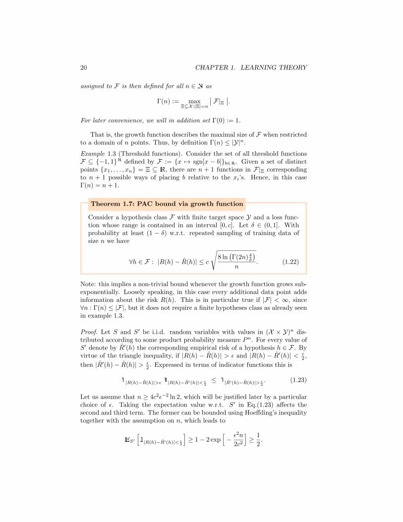
Theorem 1.7: PAC bound via growth function
Consider a hypothesis class F with finite target space Y and a loss func-tion whose range is contained in an interval [0, c]. Let δ ∈ (0, 1]. Withprobability at least (1 − δ) w.r.t. repeated sampling of training data ofsize n we have
∀h ∈ F : |R(h)− R(h)| ≤ c
√8 ln
(Γ(2n) 4
δ
)
n. (1.22)
Note: this implies a non-trivial bound whenever the growth function grows sub-exponentially. Loosely speaking, in this case every additional data point addsinformation about the risk R(h). This is in particular true if |F| < ∞, since∀n : Γ(n) ≤ |F|, but it does not require a finite hypotheses class as already seenin example 1.3.
Proof. Let S and S′ be i.i.d. random variables with values in (X × Y)n dis-tributed according to some product probability measure Pn. For every value ofS′ denote by R′(h) the corresponding empirical risk of a hypothesis h ∈ F . Byvirtue of the triangle inequality, if |R(h) − R(h)| > ε and |R(h) − R′(h)| < ε
2 ,
then |R′(h)− R(h)| > ε2 . Expressed in terms of indicator functions this is
1|R(h)−R(h)|>ε 1|R(h)−R′(h)|< ε2≤ 1|R′(h)−R(h)|> ε
2. (1.23)
Let us assume that n ≥ 4c2ε−2 ln 2, which will be justified later by a particularchoice of ε. Taking the expectation value w.r.t. S′ in Eq.(1.23) affects thesecond and third term. The former can be bounded using Hoeffding’s inequalitytogether with the assumption on n, which leads to
ES′
[1|R(h)−R′(h)|< ε
2
]≥ 1− 2 exp
[− ε2n
2c2
]≥ 1
2.
1.5. GROWTH FUNCTION 21
For the expectation value of the last term in Eq.(1.23) we use
ES′
[1|R′(h)−R(h)|> ε
2
]≤ PS′
[∃h ∈ F : |R′(h)− R(h)| > ε
2
].
Inserting both bounds into Eq.(1.23) gives
1|R(h)−R(h)|>ε ≤ 2 PS′[∃h ∈ F : |R′(h)− R(h)| > ε
2
].
As this holds for all h ∈ F , we can replace the left hand side by 1∃h∈F :|R(h)−R(h)|>ε.Taking the expectation w.r.t. S then leads to
PS
[∃h ∈ F : |R(h)− R(h)| > ε
]≤ 2PS,S′
[∃h ∈ F : |R′(h)− R(h)| > ε
2
].
Note that the r.h.s. involves only empirical quantities. This implies that everyfunction h is only evaluated on at most 2n points, namely those appearing inS and S′. Since restricted to 2n points there are at most Γ(2n) functions, ouraim is now to exploit this together with the union bound and to bound theremaining factor with Hoeffding’s inequality. To this end, observe that we canwrite
2PS,S′[∃h ∈ F : |R′(h)− R(h)| > ε
2
]= (1.24)
2ESS′
[Pσ
[∃h ∈ F :
1
n
∣∣∣n∑
i=1
(L(Yi, h(Xi)
)− L
(Y ′i , h(X ′i)
))σi
∣∣∣ > ε
2
]],
where Pσ denotes the probability w.r.t. uniformly distributed σ ∈ −1, 1n.Eq.(1.24) is based on the fact that multiplication with σi = −1 amounts to in-terchanging (Xi, Yi)↔ (X ′i, Y
′i ), which has no effect since the random variables
are independently and identically distributed. The advantage of this step is thatwe can now apply our tools inside the expectation value ESS′ where S and S′
are fixed. Then h ∈ F∣∣S∪S′ is contained in a finite function class, so that we
can use the union bound followed by an application of Hoeffding’s inequality toarrive at
PS
[∃h ∈ F : |R(h)− R(h)| > ε
]≤ 4ESS′
[∣∣F|S∪S′∣∣] exp
[−nε
2
8c2
]
≤ 4Γ(2n) exp
[−nε
2
8c2
](1.25)
The result then follows by setting the final expression in Eq.(1.25) equalto δ and solving for ε. The previously made assumption on n then becomesequivalent to δ ≤ 2
√2Γ(2n), which is always fulfilled as δ ∈ (0, 1].
Note that we have proven a slightly stronger result, in which the growthfunction Γ(2n) is replaced by ESS′
[∣∣F|S∪S′∣∣]. The logarithm of this expec-
tation value is called VC-entropy. The VC-entropy, however, depends on the
22 CHAPTER 1. LEARNING THEORY
underlying probability distribution P and is thus difficult to estimate in gen-eral. The growth function, though independent of P , may still be difficult toestimate. The following section will distill its remarkable essence for the binarycase (|Y| = 2), where Γ turns out to exhibit a simple dichotomic behavior.
For later use, let us state the behavior of the growth function w.r.t. compo-sitions:
Lemma 1.4 (Growth functions under compositions). Consider function classesF1 ⊆ YX ,F2 ⊆ ZY and F := F2 F1. The respective growth functions thensatisfy
Γ(n) ≤ Γ1(n)Γ2(n).
Proof. Fix an arbitrary subset Ξ ⊆ X of cardinality |Ξ| = n. With G := F1|Ξwe can write F|Ξ =
⋃g∈Gf g | f ∈ F2. So
∣∣F|Ξ∣∣ ≤
∣∣F1|Ξ∣∣maxg∈G
∣∣f g|f ∈ F2
∣∣
≤ Γ1(n) maxg∈G
∣∣F2|g(Ξ)
∣∣
≤ Γ1(n)Γ2(n).
1.6 VC-dimension
In the case of binary target space (|Y| = 2) there is a peculiar dichotomy in thebehavior of the growth function Γ(n). It grows at maximal rate, i.e., exponen-tially and exactly like 2n, up to some n = d and from then on remains boundedby a polynomial of degree at most d. The number d where this transition occurs,is called the VC-dimension of the function class and plays an important role inthe theory of binary classification.
Definition 1.5 (Vapnik-Chervonenkis dimension). The VC-dimension of afunction class F ⊆ YX with binary target space Y is defined as
VCdim(F) := maxn ∈ N0
∣∣ Γ(n) = 2n
if the maximum exists and VCdim(F) =∞ otherwise.
That is, if VCdim(F) = d, then there exists a set A ⊆ X of d points, suchthat F|A = YA and the VC-dimension is the largest such number.
Example 1.4 (Threshold functions). If F = R 3 x 7→ sgn[x − b]b∈R, thenVCdim(F) = 1 as we have seen in example 1.3 that Γ(n) = n+ 1. More specif-ically, if we consider an arbitrary pair of points x1 < x2, then the assignmentx1 7→ 1 ∧ x2 7→ −1 is missing in F|x1,x2. Hence, VCdim(F) < 2.

1.6. VC-DIMENSION 23
Theorem 1.8: VC-dichotomy of growth function
Consider a function class F ⊆ YX with binary target space Y and VC-dimension d. Then the corresponding growth function satisfies
Γ(n)
= 2n, if n ≤ d.≤(end
)d, if n > d.
(1.26)
Proof. Γ(n) = 2n for all n ≤ d holds by definition of the VC-dimension. In orderto arrive at the expression for n > d, we show that for every subset A ⊆ X with|A| = n the following is true:
∣∣F|A∣∣ ≤
∣∣∣B ⊆ A
∣∣ F|B = YB∣∣∣. (1.27)
If Eq.(1.27) holds, we can upper bound the r.h.s. by∣∣B ⊆ A
∣∣ |B| ≤ d∣∣ =∑d
i=0
(ni
), which for n > d in turn can be bounded by
d∑
i=0
(n
i
)≤
n∑
i=0
(n
i
)(nd
)d−i
=(nd
)d(1 +
d
n
)n≤(nd
)ded,
where the last step follows from ∀x ∈ R : (1 + x) ≤ ex. Hence, the proof isreduced to showing Eq.(1.27).
This will be done by induction on |A|. For |A| = 1 it is true (as B = ∅always counts). Now assume as induction hypothesis that it holds for all sets ofsize n− 1 and that |A| = n. Let a be any element of A and define
F ′ :=h ∈ F|A
∣∣ ∃g ∈ F|A : h(a) 6= g(a) ∧ (h− g)|A\a = 0, Fa := F ′|A\a.
Then |F|A| = |F|A\a| + |Fa| and both terms on the r.h.s. can be bounded bythe induction hypothesis. For the first term we obtain
∣∣F|A\a∣∣ ≤
∣∣∣B ⊆ A
∣∣ F|B = YB ∧ a 6∈ B∣∣∣. (1.28)
The second term can be bounded by
∣∣Fa∣∣ =
∣∣F ′|A\a∣∣ ≤
∣∣∣B ⊆ A \ a
∣∣ F ′|B = YB∣∣∣
=∣∣∣B ⊆ A \ a
∣∣ F ′|B∪a = YB∪a∣∣∣
=∣∣∣B ⊆ A
∣∣ F ′|B = YB ∧ a ∈ B∣∣∣
≤∣∣∣B ⊆ A
∣∣ F|B = YB ∧ a ∈ B∣∣∣, (1.29)
where we use the induction hypothesis in the first line and the step to thesecond line uses the defining property of F ′. Adding the bounds of Eq.(1.28)and Eq.(1.29) then yields the result claimed in Eq.(1.27).
24 CHAPTER 1. LEARNING THEORY
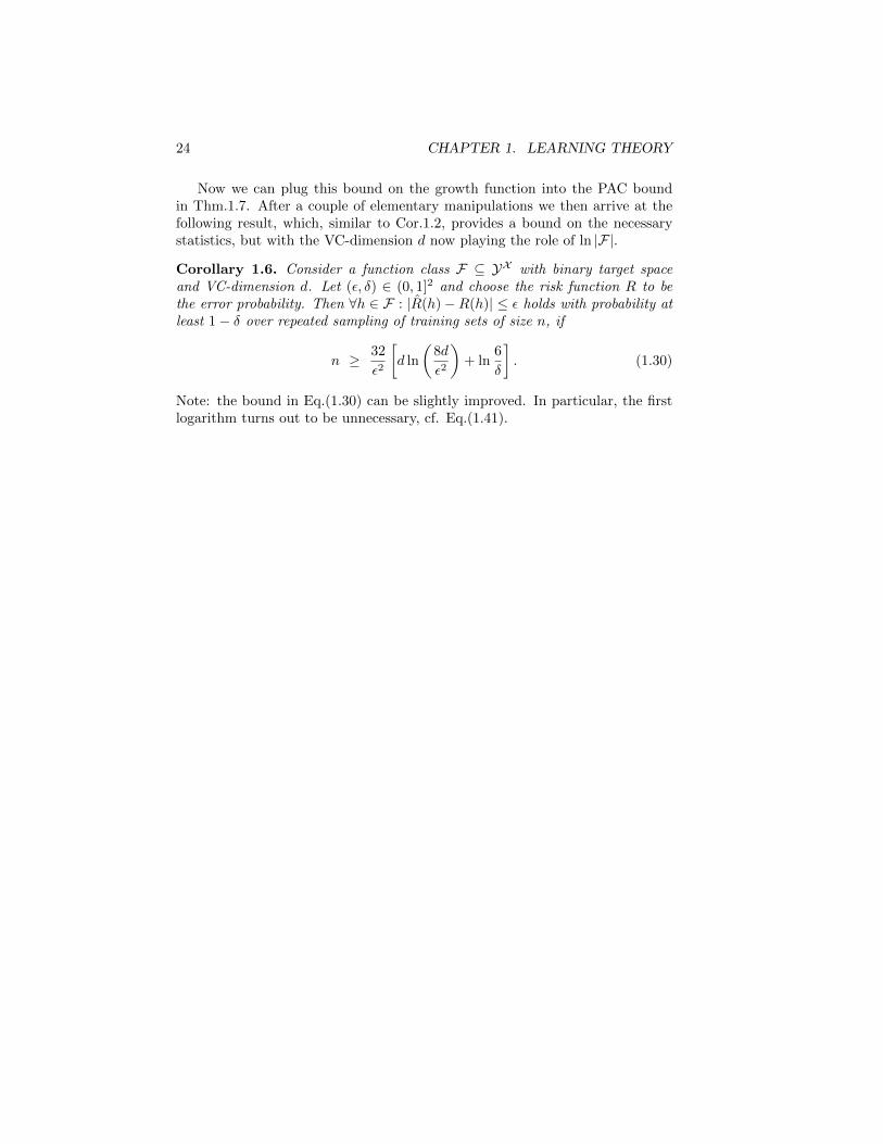
Now we can plug this bound on the growth function into the PAC boundin Thm.1.7. After a couple of elementary manipulations we then arrive at thefollowing result, which, similar to Cor.1.2, provides a bound on the necessarystatistics, but with the VC-dimension d now playing the role of ln |F|.
Corollary 1.6. Consider a function class F ⊆ YX with binary target spaceand VC-dimension d. Let (ε, δ) ∈ (0, 1]2 and choose the risk function R to bethe error probability. Then ∀h ∈ F : |R(h)−R(h)| ≤ ε holds with probability atleast 1− δ over repeated sampling of training sets of size n, if
n ≥ 32
ε2
[d ln
(8d
ε2
)+ ln
6
δ
]. (1.30)
Note: the bound in Eq.(1.30) can be slightly improved. In particular, the firstlogarithm turns out to be unnecessary, cf. Eq.(1.41).
1.6. VC-DIMENSION 25
A useful tool for computing VC-dimensions is the following theorem:
Theorem 1.9: VC-dimension for function vector spaces
Let G be a real vector space of functions from X to R and φ ∈ RX . ThenF :=
x 7→ sgn[g(x) + φ(x)]
g∈G ⊆ −1, 1X has VCdim(F) = dim(G).
Proof. Let us first prove VCdim(F) ≤ dim(G). We can assume dim(G) <∞ andargue by contradiction. Let k = dim(G) + 1 and suppose that VCdim(F) ≥ k.Then there is a subset Ξ = x1, . . . , xk ⊆ X such that F|Ξ = −1, 1Ξ. Definea map L : G → Rk via L(g) :=
(g(x1), . . . , g(xk)
). L is a linear map whose range
has dimension at most dim(G). Hence, there is a non-zero vector v ∈ (range L)⊥.This means that for all g ∈ G : 〈v, L(g)〉 = 0 and therefore
k∑
l=1
vl(g(xl) + φ(xl)
)=
k∑
l=1
vlφ(xl) (1.31)
is independent of g. However, if F|Ξ = −1, 1Ξ, we can choose g such thatsgn[g(xl) + φ(xl)] equals sgn[vl] for all l ∈ 1, . . . , k and there is also a choiceof g for which it equals −sgn[vl] for all l. Since v 6= 0 this contradicts Eq.(1.31).
In order to arrive at VCdim(F) ≥ dim(G), it suffices to show that for alld ≤ dim(G) there are points x1, . . . , xd ∈ X such that for all y ∈ Rd thereis a g ∈ G satisfying yj = g(xj) for all j. To this end, consider d linearlyindependent functions (gi)
di=1 in G and define G(x) :=
(g1(x), . . . , gd(x)
). Then
spanG(x)x∈X = Rd so that there have to exist d linearly independent vectorsG(x1), . . . , G(xd). Hence, the d × d matrix with entries gi(xj) is invertible
and for all y ∈ Rd the system of equations yj =∑di=1 γigi(xj) has a solution
γ ∈ Rd.
Corollary 1.7 (VC-dimension of half spaces). The set F :=h : Rd →
−1, 1 | ∃(v, b) ∈ Rd × R : h(x) = sgn[〈v, x〉 − b]
, which corresponds tothe set of all half spaces in Rd, satisfies
VCdim(F) = d+ 1.
Proof. The result follows from the foregoing theorem, when applied to the linearspace of functions spanned by gi(x) := xi for i = 1, . . . , d and gd+1(x) := 1 withφ = 0.
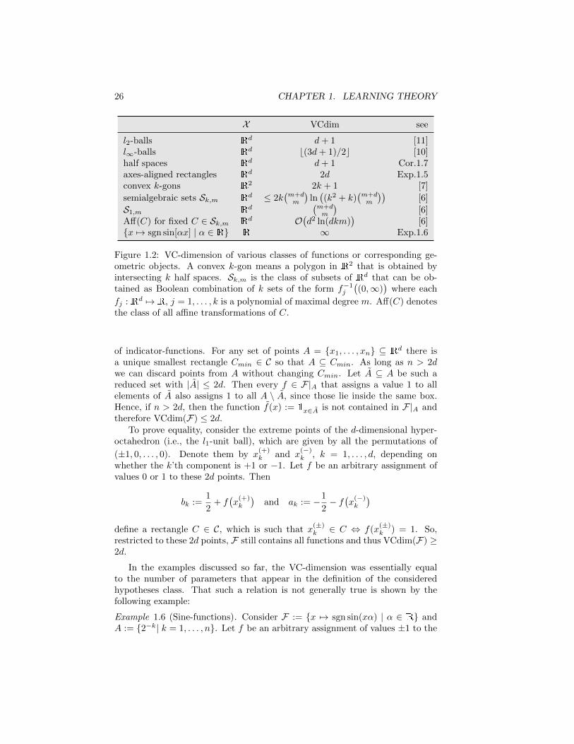
As in the case of half spaces, we can assign a function f : Rd → −1, 1 to anysubset C ⊆ Rd and vice versa via f(x) = 1⇔ x ∈ C. In this way we can applythe notion of VC-dimension to classes of Borel subsets of Rd. Table 1.2 collectssome examples.
Example 1.5 (Axes-aligned rectangles). Consider C := C ⊆ Rd|∃a, b ∈ Rd :C = [a1, b1] × . . . × [ad, bd] the set of all axes-aligned rectangles in Rd andlet F := f : Rd → 0, 1|∃C ∈ C : f(x) = 1x∈C be the corresponding class
26 CHAPTER 1. LEARNING THEORY
X VCdim see
l2-balls Rd d+ 1 [11]l∞-balls Rd b(3d+ 1)/2c [10]half spaces Rd d+ 1 Cor.1.7axes-aligned rectangles Rd 2d Exp.1.5convex k-gons R2 2k + 1 [7]
semialgebraic sets Sk,m Rd ≤ 2k(m+dm
)ln((k2 + k)
(m+dm
))[6]
S1,m Rd(m+dm
)[6]
Aff(C) for fixed C ∈ Sk,m Rd O(d2 ln(dkm)
)[6]
x 7→ sgn sin[αx] | α ∈ R R ∞ Exp.1.6
Figure 1.2: VC-dimension of various classes of functions or corresponding ge-ometric objects. A convex k-gon means a polygon in R2 that is obtained byintersecting k half spaces. Sk,m is the class of subsets of Rd that can be ob-tained as Boolean combination of k sets of the form f−1
j
((0,∞)
)where each
fj : Rd 7→ R, j = 1, . . . , k is a polynomial of maximal degree m. Aff(C) denotesthe class of all affine transformations of C.
of indicator-functions. For any set of points A = x1, . . . , xn ⊆ Rd there isa unique smallest rectangle Cmin ∈ C so that A ⊆ Cmin. As long as n > 2dwe can discard points from A without changing Cmin. Let A ⊆ A be such areduced set with |A| ≤ 2d. Then every f ∈ F|A that assigns a value 1 to allelements of A also assigns 1 to all A \ A, since those lie inside the same box.Hence, if n > 2d, then the function f(x) := 1x∈A is not contained in F|A andtherefore VCdim(F) ≤ 2d.
To prove equality, consider the extreme points of the d-dimensional hyper-octahedron (i.e., the l1-unit ball), which are given by all the permutations of
(±1, 0, . . . , 0). Denote them by x(+)k and x
(−)k , k = 1, . . . , d, depending on
whether the k’th component is +1 or −1. Let f be an arbitrary assignment ofvalues 0 or 1 to these 2d points. Then
bk :=1
2+ f
(x
(+)k
)and ak := −1
2− f
(x
(−)k
)
define a rectangle C ∈ C, which is such that x(±)k ∈ C ⇔ f(x
(±)k ) = 1. So,
restricted to these 2d points, F still contains all functions and thus VCdim(F) ≥2d.
In the examples discussed so far, the VC-dimension was essentially equalto the number of parameters that appear in the definition of the consideredhypotheses class. That such a relation is not generally true is shown by thefollowing example:
Example 1.6 (Sine-functions). Consider F := x 7→ sgn sin(xα) | α ∈ R andA := 2−k| k = 1, . . . , n. Let f be an arbitrary assignment of values ±1 to the
1.6. VC-DIMENSION 27
points xk := 2−k in A. If we choose
α := π
(1 +
n∑
k=1
1− f(xk)
22k
), we obtain
α xl mod 2π = π
(1− f(xl)
2
)+ π
[2−l +
l−1∑
k=1
2k−l(
1− f(xk)
2
)]
=: π
(1− f(xl)
2
)+ π c, (1.32)
where c ∈ (0, 1). Consequently, sgn sin(αxl) = f(xl) and thus F|A = −1, 1A.Since this holds for all n, we have VCdim(F) = ∞ despite the fact that thereis only a single real parameter involved.
Although the VC-dimension is infinite in this example, there are finite setsB for which F|B 6= −1, 1B . Consider for instance B := 1, 2, 3, 4 and theassignment f(1) = f(2) = −f(3) = f(4) = −1. If α = 2πm − δ, m ∈ N withδ ∈ [0, 2π) is to reproduce the first three values, then δ ∈ [π/3, π/2). However,this implies that 4δ is in the range where the sine is positive, so that f(4) = −1cannot be matched.
Let us finally have a closer look at sets of functions from Euclidean space to0, 1 that are constructed using Boolean combinations of few elementary, forinstance polynomial, relations. In this context, it turns out that VC-dimensionand growth function are related to the question how many connected compo-nents can be obtained when partitioning Euclidean space using these relations.Loosely speaking, counting functions becomes related to counting cells in thedomain space. A central bound concerning the latter problem was derived byWarren for the case of polynomials:
Proposition 1.8 (Warren’s upper bound for polynomial arrangements). Letp1, . . . , pm be a set of m ≥ k polynomials in k variables, each of degree atmost d and with coefficients in R. Let γ(k, d,m) be the number of connectedcomponents of Rk \
⋃mi=1 p
−1(0) (and for later use, let us define it to be thelargest number constructed in this way). Then
γ(k, d,m) ≤ (4edm/k)k. (1.33)
With this ingredient, we can obtain the following result. To simplify itsstatement, predicates are interpreted as functions into 0, 1, i.e., we identifyTRUE = 1 and FALSE = 0.
Theorem 1.10: Complexity of semi-algebraic function classes
Let d, k,m, s ∈ N. Consider a set of s atomic predicates, each of which isgiven by a polynomial equality or inequality of degree at most d in m+ kvariables. Let Ψ : Rm × Rk → 0, 1 be a Boolean combination of theatomic predicates and F := Ψ(·, w) | w ∈ Rk a class of functions from
28 CHAPTER 1. LEARNING THEORY
Rm into 0, 1 with corresponding growth function Γ. Then
Γ(n) ≤ γ(k, d, 2ns) , (1.34)
V Cdim(F) ≤ 2k log2(8eds) . (1.35)
Proof. W.l.o.g. we assume that all polynomial (in-)equalities are comparisonswith zero, i.e., of the form p#0 where p is a polynomial and # ∈ <,≤,=,≥, >.We are going to estimate |F|A| for a set A ⊂ Rm with cardinality |A| = n.Each a ∈ A corresponds to a predicate ψa : Rk → 0, 1 that is definedby ψa(w) := Ψ(a,w). Denote by Pa the set of polynomials (in the variablesw1, . . . , wk) that appear in ψa. Then P :=
⋃a∈A Pa has cardinality |P | ≤ ns.
Since different functions in F|A correspond to different truth values of the poly-nomial (in-)equalities, we have that the number of consistent sign-assignmentsto the polynomials in P is an upper bound on the number of function in F|A.That is,
|F|A| ≤∣∣∣Q ∈ −1, 0, 1P
∣∣ Q(p) = sgn0
(p(w)
), w ∈ Rk
∣∣∣, (1.36)
where sgn0 := sgn on R\0 and sgn0(0) := 0. For ε > 0 define P ′ := p+ε|p ∈P ∪ p − ε|p ∈ P. Then |P ′| ≤ 2|P | ≤ 2ns and if ε is sufficiently small, thenumber of consistent sign-assignments for P is upper bounded by the numberof connected components of Rk \
⋃p∈P ′ p
−1(0). Hence, |F|A| ≤ γ(k, d, |P ′|),which implies Eq.(1.34).
The bound on the VC-dimension in Eq.(1.35) then combines this result withProp.1.8. If n equals the VC-dimension of F , then 2n = Γ(n) ≤ γ(k, d, 2ns) ≤(8edns/k)k. Here, the last inequality used Prop.1.8 assuming that 2ns ≥ k.Note, however, that if 2ns < k, then Eq.(1.35) holds trivially. After taking thelog2, we arrive at the inequality
n ≤ k log2(8eds) + k log2(n/k).
If the second term on the r.h.s. is smaller than the first, Eq.(1.35) followsimmediately. If, on the other hand, n/k ≥ 8eds, then n ≤ 2k log2(n/k), whichin turn implies n ≤ 4k and Eq.(1.35) follows, as well.
Note that the first part of the proof, which relates the growth function to thenumber of connected components of a particular partitioning of Rk, made noessential use of the fact that the underlying functions are polynomials. Thatmeans, all one needs is a sufficiently well-behaved class of functions for which‘cell counting’ can be done in the domain space.
An alternative view on the problem is in terms of the computational com-plexity of Ψ. By assumption, the function Ψ in Thm.1.10 can be computedusing few elementary arithmetic operations and conditioning on (in-)equalities.The number of these operations is then related to d and s. A closer analysis ofthis point of view leads to:
1.7. FUNDAMENTAL THEOREM OF BINARY CLASSIFICATION 29
Theorem 1.11: VC-dimension from computational complexity
Assume Ψ : Rm×Rk → 0, 1 can be computed by an algorithm that exe-cutes at most t of the following operations: (i) basic arithmetic operations(×, /,+,−) on real numbers, (ii) jumps conditioned on equality or inequal-ity of real numbers, (iii) output 0 or 1. Then F := Ψ(·, w) | w ∈ Rksatisfies
V Cdim(F) ≤ 2k(2t+ log2 8e
). (1.37)
This follows from Thm.1.10 by realizing that the algorithm corresponds to analgebraic decision tree with at most 2t leaves and that it can be expressed interms of ≤ 2t polynomial predicates of degree ≤ 2t.
With some effort one can add one further type to the list of operations thealgorithm for Ψ is allowed to execute: computation of the exponential functionon real numbers. Under these conditions the upper bound then becomes
V Cdim(F) = O(t2k2
). (1.38)
1.7 Fundamental theorem of binary classifica-tion
In this section we collect the insights obtained so far and use them to provewhat may be called the fundamental theorem of binary classification. For itsformulation, denote by poly
(1ε ,
1δ
)the set of all functions of the form (0, 1] ×
(0, 1] 3 (ε, δ) 7→ ν(ε, δ) ∈ R+ that are polynomial in 1ε and 1
δ .
Theorem 1.12: Fundamental theorem of binary classification
Let F ⊆ −1, 1X be any hypotheses class and n = |S| the size of thetraining data set S, which is treated as a random variable, distributed ac-cording to some product probability measure Pn. Choose the risk functionR to be the error probability. Then the following are equivalent:
1. (Finite VC-dimension) VCdim(F) <∞.
2. (Uniform convergence) There is a ν ∈ poly(
1ε ,
1δ
)so that for all
(ε, δ) ∈ (0, 1]2 and all probability measures P we have
n ≥ ν(ε, δ) ⇒ PS
[∃h ∈ F : |R(h)−R(h)| ≥ ε
]≤ δ.
3. (PAC learnability) There is a ν ∈ poly(
1ε ,
1δ
)and a learning algo-
rithm that maps S 7→ hS ∈ F so that for all (ε, δ) ∈ (0, 1]2 and allprobability measures P we have
n ≥ ν(ε, δ) ⇒ PS [|R(hS)−RF | ≥ ε] ≤ δ. (1.39)

30 CHAPTER 1. LEARNING THEORY
4. (PAC learnability via ERM) There is a ν ∈ poly(
1ε ,
1δ
)so that
for all (ε, δ) ∈ (0, 1]2 and all probability measures P we have
n ≥ ν(ε, δ) ⇒ PS
[|R(h)−RF | ≥ ε
]≤ δ,
where h ∈ F is an arbitrary empirical risk minimizer.
Proof. 1.⇒ 2. is the content of Cor.1.6.2.⇒ 4.: Assuming uniform convergence, with probability at least (1− δ) we
have that ∀h ∈ F : |R(h) − R(h)| ≤ ε2 if n ≥ ν( ε2 , δ). By Eq.(1.7) this implies
R(h)−RF ≤ ε.4.⇒ 3. is obvious since the former is a particular instance of the latter.3. ⇒ 1. is proven by contradiction: choose ε = δ = 1/4, n = ν(ε, δ) and
suppose VCdim(F) = ∞. Then for any N ∈ N there is a subset Ξ ⊆ X ofsize |Ξ| = N such that F|Ξ = −1, 1Ξ. Applying the no-free-lunch theorem tothis space we get that there is an f : Ξ → −1, 1, which defines a probabilitydensity P (x, y) := 1x∈Ξ ∧ f(x)=y/N on X × −1, 1 with respect to which
ES [R(hS)] ≥ 1
2
(1− n
N
)(1.40)
holds for an arbitrary learning algorithm, given by a mapping S 7→ hS . Usingthat R(hS) is itself a probability and thus bounded by one, we can bound
ES [R(hS)] ≤ 1 ·PS [R(hS) ≥ ε] + ε(1−PS [R(hS) ≥ ε]
).
Together with Eq.(1.40) and ε = 14 this leads to PS
[R(hS) ≥ 1
4
]≥ 1
3 −2n3N ,
which for sufficiently large N contradicts δ = 14 .
There is also a quantitative version of this theorem. In fact, the VC-dimension does not only lead to a bound on the necessary statistics, it preciselyspecifies the optimal scaling of ν. Let us denote by νF the pointwise infimum ofall functions ν taken i) over all functions for which the implication in Eq.(1.39)is true for all P and all (ε, δ) and ii) over all learning algorithms with range F .νF is called the sample complexity of F and it can be shown that
νF (ε, δ) = Θ
(VCdim(F) + ln 1
δ
ε2
). (1.41)
Here, the asymptotic notation symbol Θ means that there are asymptotic upperand lower bounds that differ only by multiplicative constants (that are non-zeroand finite).
Note that the scaling in 1/δ is much better than required—logarithmic ratherthan polynomial. Hence, we could have formulated a stronger version of thefundamental theorem. However, requiring polynomial scaling is what is typicallydone in the general definition of PAC learnability.
What about generalizations to cases with |Y| > 2? For both, classification(Y discrete) and regression (Y continuous), the concept of VC-dimension has
1.8. RADEMACHER COMPLEXITY 31
been generalized and there exist various counterparts to the VC-dimension withsimilar implications. For the case of classification, the graph dimension dGand the Natarajan dimension dN are two useful generalizations that lead toquantitative bounds on the sample complexity of a hypotheses class with theerror probability as risk function. In the binary case they both coincide withthe VC-dimension, while in general dN ≤ dG ≤ 4.67dN log2 |Y| (cf. [5]). Knownbounds on the sample complexity νF turn out to have still the form of Eq.(1.41)with the only difference that in the upper and lower bound the role of the VC-dimension is played by dG and dN , respectively. The logarithmic gap betweenthe two appears to be relevant and leads to the possibility of good and badERM learning algorithms (cf. [9]).
In the case of regression, a well-studied counterpart of the VC-dimensionis the fat-shattering dimension. For particular loss functions (e.g., the squaredloss) the above theorem then has a direct analogue, in the sense that undermild assumptions, uniform convergence, finite fat-shattering dimension and PAClearnability are equivalent [3]. In general learning contexts, however, uniformconvergence turns out to be a strictly stronger requirement than PAC learnabil-ity [22, 9].
1.8 Rademacher complexity
The approaches discussed so far were distribution independent. Growth functionand VC-dimension, as well as its various generalizations, depend only on thehypotheses class F and lead to PAC guarantees that are independent of theprobability measures P . In this section we will consider an alternative approachand introduce the Rademacher complexities. These will not only depend onF , but also on P or, alternatively, on the empirical distribution given by thedata. This approach has several possible advantages compared to what wehave discussed before. First, a data dependent approach may, in benign cases,provide better bounds than a distribution-free approach that has to cover theworst case, as well. Second, the approach based on Rademacher complexitiesallows us to go beyond binary classification and treat more general functionclasses that appear in classification or regression problems on an equal footing.
Definition 1.9 (Rademacher complexity). Consider a set of real-valued func-tions G ⊆ RZ and a vector z ∈ Zn. The empirical Rademacher complexity ofG w.r.t. z is defined as
R(G) := Eσ
[supg∈G
1
n
n∑
i=1
σig(zi)
], (1.42)
where Eσ denotes the expectation w.r.t. a uniform distribution of σ ∈ −1, 1n.If the zi’s are considered values of a vector of i.i.d.random variables Z :=(Z1, . . . , Zn), each distributed according to a probability measure P on Z, thenthe Rademacher complexities of G w.r.t. P are given by
Rn(G) := EZ
[R(G)
]. (1.43)
32 CHAPTER 1. LEARNING THEORY
Note: The uniformly distributed σi’s are called Rademacher variables. When-ever we want to emphasize the dependence of R(G) on z ∈ Zn, we will writeRz(G). Similarly, we occasionally write Rn,P (G) to make the dependence on Pexplicit. We will tacitly assume that G is chosen so that the suprema appearingin the definition lead to measurable functions.
The richer the function class G, the larger the (empirical) Rademacher com-plexity. If we define g(z) :=
(g(z1), . . . , g(zn)
)and write
R(G) =1
nEσ
[supg∈G〈σ, g(z)〉
],
we see that the (empirical) Rademacher complexity measures how well the func-tion class G can ’match Rademacher noise’. If for a random sign pattern σ thereis always a function in G that is well aligned with σ in the sense that 〈σ, g(z)〉 islarge, the Rademacher complexity will be large. Clearly, this will become moreand more difficult when the number n of considered points is increased.
With the following Lemma, which is a refinement of Hoeffding’s inequality,we can show that the Rademacher complexity is close to its empirical counter-part. This will imply that the Rademacher complexity can be estimated reliablyfrom the data and that no additional knowledge about P is required.
Lemma 1.10 (McDiarmid’s inequality[19]). Let (Z1, . . . , Zn) = Z be a finitesequence of independent random variables, each with values in Z and ϕ : Zn →R a measurable function such that |ϕ(z) − ϕ(z′)| ≤ νi whenever z and z′ onlydiffer in the i’th coordinate. Then for every ε > 0
P[ϕ(Z)−E [ϕ(Z)] ≥ ε
]≤ exp
[− 2ε2∑n
i=1 ν2i
]. (1.44)
Note: the same inequality holds with ϕ(Z) and E [ϕ(Z)] interchanged. Thiscan be seen by replacing ϕ with −ϕ.
Lemma 1.11 (Rademacher vs. empirical Rademacher complexity). Let G ⊆[a, b]Z be a set of real-valued functions. Then for every ε > 0 and any productprobability measure Pn on Zn it holds that
PZ
[(Rn(G)− RZ(G)
)≥ ε]≤ exp− 2nε2
(b− a)2. (1.45)
Proof. Define ϕ : Zn → R as ϕ(z) := Rz(G), which implies E [ϕ(Z)] =Rn(G). Let z, z′ ∈ Zn be a pair that differs in only one component. Thensupg∈G
∑i σig(zi) changes by at most |b−a| if we replace z by z′. Consequently,
|ϕ(z)− ϕ(z′)| = |Rz(G)− Rz′(G)| ≤ |b− a|n
, (1.46)
and we can apply McDiarmid’s inequality to obtain the stated result.
Now we are prepared for the main result of this section and can prove aPAC-type guarantee based on (empirical) Rademacher complexities:
1.8. RADEMACHER COMPLEXITY 33
Theorem 1.13: PAC-type bound via Rademacher complexities
Consider arbitrary spaces X ,Y, a hypotheses class F ⊆ YX , a loss func-tion L : Y × Y → [0, c] and define Z := X × Y and G := (x, y) 7→L(y, h(x)) | h ∈ F ⊆ [0, c]Z . For any δ > 0 and any probability measureP on Z we have with probability at least (1− δ) w.r.t. repeated samplingof Pn-distributed training data S ∈ Zn: all h ∈ F satisfy
R(h)− R(h) ≤ 2Rn(G) + c
√ln 1
δ
2n, and (1.47)
R(h)− R(h) ≤ 2RS(G) + 3c
√ln 2
δ
2n. (1.48)
Proof. Defining ϕ : Zn → R as ϕ(S) := suph∈F(R(h) − R(h)
), we can apply
McDiarmid’s inequality to ϕ with νi = cn and obtain
PS [ϕ(S)−ES [ϕ(S)] ≥ ε] ≤ e−2nε2/c2 .
Setting the r.h.s. equal to δ and solving for ε then gives that with probabilityat least 1− δ we have
suph∈F
(R(h)− R(h)
)≤ ES [ϕ(S)] + c
√ln 1
δ
2n. (1.49)
It remains to upper bound the expectation on the right. To this end, we willagain introduce a second sample S′ that is an i.i.d. copy of S. Then
ES [ϕ(S)] = ES
[suph∈F
1
n
n∑
i=1
ES′[L(Y ′i , h(X ′i)
)− L
(Yi, h(Xi)
)]]
≤ ESS′
[suph∈F
1
n
n∑
i=1
L(Y ′i , h(X ′i)
)− L
(Yi, h(Xi)
)]
= ESS′Eσ
[suph∈F
1
n
n∑
i=1
σi
(L(Y ′i , h(X ′i)
)− L
(Yi, h(Xi)
))]
≤ 2 ESEσ
[suph∈F
1
n
n∑
i=1
σiL(Yi, h(Xi)
)]
= 2Rn(G),
where between the second and third line we have used that multiplication withσi = −1 amounts to interchanging (Xi, Yi) ↔ (X ′i, Y
′i ), which has no effect as
these are i.i.d. random variables. This proves Eq.(1.47). In order to obtainEq.(1.48) note that by Lemma 1.11 with probability at least 1− δ/2 we have
Rn(G) ≤ R(G) + c
√ln 2
δ
2n.
34 CHAPTER 1. LEARNING THEORY
Combining this via the union bound with Eq.(1.47), where the latter is alsoapplied to δ/2 instead of δ, then yields the desired result.
When applying the previous theorem to the case of binary classification, onecan replace the Rademacher complexities of G by those of the hypotheses classF :
Lemma 1.12 (Rademacher complexities for binary classification). Consider ahypotheses class F ⊆ −1, 1X , L(y, y′) := 1y 6=y′ as loss function and G :=(x, y) 7→ L(y, h(x)) | h ∈ F. Denote the restriction of S =
((xi, yi)
)ni=1∈
(X × −1, 1)n to X by SX := (xi)ni=1. For any probability measure P on
X × −1, 1 with marginal p on X we have
RS(G) =1
2RSX (F) and Rn,P (G) =
1
2Rn,p(F). (1.50)
Proof. The second equation is obtained from the first by taking the expectationvalue. The first is obtained by exploiting that L(y, h(x)) = (1−yh(x))/2. Then
RS(G) = Eσ
[suph∈F
1
n
n∑
i=1
σi(1− yih(xi)
)/2
]
=1
2Eσ
[suph∈F
1
n
n∑
i=1
σih(xi)
]=
1
2RSX (F),
where we have used that Eσ [σi] = 0 and that the distributions of −σiyi and σiare the same.
If, similar to the last part of the proof, we use that σi and −σi are equallydistributed, we can write
RSX (F) = Eσ
[suph∈F
1
n
n∑
i=1
−σih(xi)
]= −Eσ
[infh∈F
1
n
n∑
i=1
σih(xi)
].
Hence, computing the empirical Rademacher complexity is an optimizationproblem similar to empirical risk minimization—so it may be hard. The Rademachercomplexity Rn itself depends on an unknown distribution and is therefore diffi-cult to estimate, as well. However, it can be bounded for instance in the binarycase in terms of the growth function or the VC-dimension. More specifically,
Rn(F) ≤√
2 ln Γ(n)
nand Rn(F) ≤ C
√VCdim(F)
n, (1.51)
for some universal constant C. These inequalities will be proven in Cor.1.14and Cor.1.21.
Before going there, let us collect some properties of the Rademacher com-plexities and a Lemma, which turn out to be useful for their application andestimation.
1.8. RADEMACHER COMPLEXITY 35
Theorem 1.14: Properties of Rademacher complexities
Let G,G1,G2 ⊆ RZ be classes of real-valued functions on Z and z ∈ Zn.The following holds for the empirical Rademacher complexities w.r.t. z:
1. If c ∈ R, then R(cG) = |c|R(G).
2. G1 ⊆ G2 implies R(G1) ≤ R(G2).
3. R(G1 + G2) = R(G1) + R(G2).
4. R(G) = R(conv G), where conv denotes the convex hull.
5. If ϕ : R→ R is L−Lipschitz, then R(ϕ G) ≤ L R(G).
Proof. (sketch) 1.-3. follow immediately from the definition.4. follows from the simple observation that
supλ∈Rm+ ,||λ||1=1
n∑
i=1
m∑
l=1
λlσigl(zi) = maxl∈1,...,m
n∑
i=1
σigl(zi).
5. Define V := v ∈ Rn | ∃g ∈ G ∀i : vi = g(zi). Then
nR(ϕ G) = Eσ
[supv∈V
n∑
i=1
σiϕ(vi)
](1.52)
=1
2Eσ2,...,σn
[supv,v′∈V
ϕ(v1)− ϕ(v′1) +
n∑
i=2
σi(ϕ(vi) + ϕ(v′i)
)]
≤ 1
2Eσ2,...,σn
[supv,v′∈V
L|v1 − v′1|+n∑
i=2
σi(ϕ(vi) + ϕ(v′i)
)]
= Eσ
[supv∈V
Lσ1v1 +
n∑
i=2
σiϕ(vi)
], (1.53)
where in the last step we used that the absolute value can be dropped since theexpression is invariant w.r.t. interchanging v ↔ v′. Repeating the above stepsfor the other n− 1 components then leads to the claimed result.
Remark: sometimes the definition of the (empirical) Rademacher complexity inthe literature differs from the one in Eqs.(1.42, 1.43) and the absolute value istaken, i.e., the empirical quantity is defined as Eσ
[supg
∣∣∑i σig(xi)
∣∣] instead.In this case Thm.1.14 essentially still holds with small variations: then 3. be-comes an inequality ’≤’ and 5. requires in addition that ϕ(−z) = −ϕ(z) (see[1]).
Lemma 1.13 (Massart’s Lemma). Let A be a finite subset of Rm that is con-tained in a Euclidean ball of radius r. Then
Eσ
[maxa∈A
m∑
i=1
σiai
]≤ r√
2 ln |A|, (1.54)
36 CHAPTER 1. LEARNING THEORY
where the expectation value is w.r.t. uniformly distributed Rademacher variablesσ ∈ −1, 1m.
Proof. W.l.o.g. we can assume that the center of the ball is at the origin sinceEq.(1.54) is unaffected by a translation. We introduce a parameter λ > 0 to bechosen later and first compute an upper bound for the rescaled set λA:
Eσ
[maxa∈λA
m∑
i=1
σiai
]≤ Eσ
[ln∑
a∈λA
eσ·a
]≤ lnEσ
[∑
a∈λA
eσ·a
](1.55)
= ln∑
a∈λA
m∏
i=1
eai + e−ai
2(1.56)
≤ ln∑
a∈λA
e||a||22/2 ≤ 1
2r2λ2 + ln |A|. (1.57)
Here, the first step is most easily understood when taking the exponential onboth sides of the inequality for a fixed value of σ. Then the first inequality inEq.(1.55) reduces to the statement that the maximum over positive numberscan be upper bounded by their sum. The second inequality uses concavity ofthe logarithm together with Jensen’s inequality. Eq. (1.56) uses that the σi’sare independently and uniformly distributed. The step to Eq.(1.57) exploits
that ex + e−x ≤ 2ex2/2 holds for all x ∈ R. The final inequality then bounds
the sum by its maximal element multiplied by the number of terms.We then obtain the claimed result by inserting λ =
√2 ln |A|/r into
Eσ
[maxa∈A
m∑
i=1
σiai
]≤(
1
2r2λ2 + ln |A|
)/λ.
We can now use this Lemma to prove the claimed relation between theRademacher complexities and the growth function of a function class:
Corollary 1.14 (Growth function bound on Rademacher complexity). Let Y ⊂R be a finite set of real numbers of modulus at most c > 0. The Rademachercomplexity of any function class G ⊆ YX can then be bounded in terms of itsgrowth function by
Rn(G) ≤ c√
2 ln Γ(n)
n. (1.58)
Proof. The statement follows directly from Massart’s Lemma (Lem. 1.13) to-gether with the fact that ||z||2 ≤ c
√n if z := (g(x1), . . . , g(xn)) for some g ∈ G
and x ∈ Xn. Using r := c√n in Massart’s Lemma then gives
Rn(G) = EZEσ supg∈G
1
n
n∑
i=1
σig(xi)
≤ r
n
√2 ln Γ(n) = c
√2 ln Γ(n)
n.
1.9. COVERING NUMBERS 37
1.9 Covering numbers
Rademacher complexities, growth function and VC dimension all exploit someform of discretization in order to quantify the complexity of a function class.In this section, we will follow an approach that makes this more explicit: wequantify complexity of a function class directly in terms of the minimal numberof discretization points that is necessary to approximate any function in theclass to a given degree. The obtained covering and packing numbers will thenturn out to be a useful tool for deriving generalization bounds. For instance, ingeneralizing the concept of the growth function or in enabling improved boundson Rademacher complexities.
Definition 1.15 (Coverings and packings). Let (M, d) be a pseudometric space5,A,B ⊆M and ε > 0.
• A is called ε-cover of B if ∀b ∈ B ∃a ∈ A : d(a, b) ≤ ε. It is called aninternal cover if in addition A ⊆ B. The ε-covering number of B, denotedby N(ε, B), is the smallest cardinality of any ε-cover of B. If only internalcovers are considered, we will write Nin(ε, B).
• A ⊆ B is called an ε-packing of B if a, b ∈ A ⇒ d(a, b) > ε. The ε-packing number of B, denoted by M(ε, B), is the largest cardinality ofany ε-packing of B.
Note that by definition Nin(ε, B) ≥ N(ε, B). In fact, all those numbers areclosely related:
Lemma 1.16 (Packing vs. covering). For every pseudometric space (M, d) andB ⊆M:
N(ε/2, B) ≥M(ε, B) ≥ Nin(ε, B).
Proof. Assume that A ⊆ B is a maximal ε-packing of B, i.e. such that no morepoint can be added to A without violating the ε-packing property. Then forevery b ∈ B there is an a ∈ A s.t. d(a, b) ≤ ε. Hence, A is an internal ε-cover ofB and therefore M(ε, B) ≥ Nin(ε, B).
Conversely, let C be a smallest ε/2-cover of B, i.e. |C| = N(ε/2, B). If Ais an ε-packing of B, then the ball b ∈ B | d(c, b) < ε/2 around any c ∈ Ccontains at most one element from A: if there were two elements a, a′ ∈ A, thend(a, a′) ≤ d(a, c) + d(c, a′) < ε would contradict the ε-packing assumption. So|C| ≥ |A| and thus N(ε/2, B) ≥M(ε, B).
One way of thinking about these numbers in terms of the number of bitsthat are required to specify any point up to a given error:
5A pseudometric space lacks only one property to a metric space: distinct points are notrequired to have distance zero.
38 CHAPTER 1. LEARNING THEORY
Proposition 1.17 (Information encoding vs. covering numbers). Let A be asubset of a metric space (M,d) and β(ε, A) the smallest number of bits sufficientto specify every a ∈ A up to an error of at most ε in the metric. That is, thesmallest n, such that there is a γ : 0, 1n → A so that ∀a ∈ A∃b ∈ 0, 1n :d(γ(b), a) ≤ ε. Then
log2N(ε, A) ≤ β(ε, A) ≤ dlog2M(ε, A)e.
Proof. If n = β(ε, A), then there is as assignment A 3 a 7→ γ(b(a)) that is ε-close to a. Hence, the range of γ is an ε-cover of A, which implies N(ε, A) ≤ 2n
proving the lower bound.For the upper bound, assume that x1, . . . , xM ⊆ A is a maximal ε-packing
of A and set n := dlog2Me. Then we can choose b = b(a) to be the binaryrepresentation of i = argminid(a, xi) and define γ(b) := xi. If there would be ana with d(γ(b), a) > ε, by construction, d(xj , a) > ε had to hold for all j, whichcontradicts the assumption that we started with a maximal ε-packing.
Example 1.7 (Norm balls in Rd). Let || · || be any norm on Rd, Br(x) := z ∈Rd| ||z−x|| ≤ r and x1, . . . , xM ⊂ Rd a maximal ε-packing of Br(0). That is,w.r.t. the metric induced by the norm we have M = M(ε, Br(0)). Then the ballsBε/2(xi) are mutually disjoint and lie inside Br+ε/2(0). If v := vol(B1(0)) is the
volume (i.e., Lebesgue measure) of the unit ball, then vol(Bε/2(xi)) = (ε/2)dv
and vol(Br+ε/2(0)) = (r+ε/2)dv. So under the assumption that ε ≤ r we obtainthe bound:
M(ε, Br(0)
)≤ (r + ε/2)dv
(ε/2)dv≤(
3r
ε
)d. (1.59)
In a similar way, we can obtain a lower bound from the simple fact that thevolume of Br(0) is upper bounded by the volume of an ε-ball times the ε-coveringnumber N(ε, Br(0)). Hence,
N(ε, Br(0)) ≥(rε
)d.
This examples exhibits a typical behavior of covering and packing numbers:the ε-packing number of a bounded object B of algebraic dimension d typicallyscales as6
lnM(ε, B) ∼ d ln1
ε.
One of the central observations when using covering and packing numbers inthe context of statistical learning theory is that this relation still holds whenthe algebraic dimension is replaced by a combinatorial dimension, such as theVC-dimension. One bound of this type is the content of the subsequent Lemma.In order to state it, we first need to introduce the metrics with respect to whichthe covering and packing numbers will be considered. For any set Z, z ∈ Zn
6In fact, this can be used to define a dimension (which is then called Minkowski-dimension),for fractal objects or metric spaces where no algebraic notion of dimension exists.
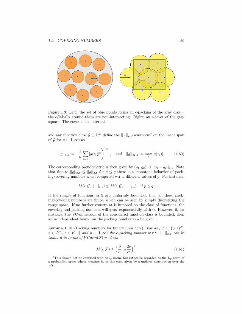
1.9. COVERING NUMBERS 39
/2
Figure 1.3: Left: the set of blue points forms an ε-packing of the gray disk—the ε/2-balls around them are non-intersecting. Right: an ε-cover of the graysquare. The cover is not internal.
and any function class G ⊆ RZ define the || · ||p,z-seminorm7 on the linear spanof G for p ∈ [1,∞) as
||g||p,z :=
(1
n
n∑
i=1
|g(zi)|p)1/p
, and ||g||∞,z := maxi|g(zi)|. (1.60)
The corresponding pseudometric is then given by (g1, g2) 7→ ||g1 − g2||p,z. Notethat due to ||g||p,z ≤ ||g||q,z for p ≤ q there is a monotone behavior of pack-ing/covering numbers when computed w.r.t. different values of p. For instance,
M(ε,G, || · ||p,z) ≤M(ε,G, || · ||q,z) if p ≤ q.
If the ranges of functions in G are uniformly bounded, then all these pack-ing/covering numbers are finite, which can be seen by simply discretizing therange space. If no further constraint is imposed on the class of functions, thecovering and packing numbers will grow exponentially with n. However, if, forinstance, the VC-dimension of the considered function class is bounded, thenan n-independent bound on the packing number can be given:
Lemma 1.18 (Packing numbers for binary classifiers). For any F ⊆ 0, 1X ,x ∈ Xn, ε ∈ (0, 1] and p ∈ [1,∞) the ε-packing number w.r.t. || · ||p,x can bebounded in terms of V Cdim(F) =: d via
M(ε,F) ≤( 9
εpln
2e
εp
)d. (1.61)
7This should not be confused with an lp-norm, but rather be regarded as the Lp-norm ofa probability space whose measure is, in this case, given by a uniform distribution over thezi’s.
40 CHAPTER 1. LEARNING THEORY
Proof. It suffices to prove the statement for p = 1. Due to the particular binarytarget space, the general case follows from ||f1 − f2||pp,x = ||f1 − f2||1,x, whichimplies M(ε,F , || · ||p,x) = M(εp,F , || · ||1,x).
Let f1, . . . , fM ⊆ F be a maximal ε-packing of F . That is, for all k 6= l:||fk−fl||1,x > ε and M = M(ε,F). Note that ||fk−fl||1,x can be interpreted asthe probability that fk(xi) 6= fl(xi) when xi is drawn uniformly from x (whenthe latter is regarded as an n-element set). So if A is a random m-tuple withi.i.d. entries from x, then PA[fk|A = fl|A] ≤ (1− ε)m ≤ e−mε. Using the unionbound, this leads to
PA
[∃k, l : k 6= l ∧ fk|A = fl|A
]< M2e−mε.
If this probability is smaller than one, as it is the case when m ≥ 2ε lnM , then
there is an A on which all fk’s differ. This implies that F|A contains at leastM different functions and therefore M ≤ Γ(m). Using that Γ(m) ≤ (em/d)d
(Thm.1.8) and inserting m = 2ε lnM this can be written as
M1/d ≤ 2e
εlnM1/d. (1.62)
Exploiting that a ≤ b ln a⇒ a ≤ (1−1/e)−1b ln b and applying it with a = M1/d,
b = 2e/ε to Eq.(1.62) then leads to M ≤(
9ε ln 2e
ε
)d.
The ε-dependence of the bound in Eq.(1.61) can be improved to
M(ε,F) ≤ e(d+ 1)
(2e
εp
)d. (1.63)
The non-trivial proof of this improvement can be found in [?].Another particular function class for which we derive an upper bound on
covering numbers is the class of bounded linear functions. A useful tool in thiscontext is a beautiful application of the ‘probabilistic method’, which yields thefollowing approximate version of Caratheodory’s theorem:
Lemma 1.19 (Maurey’s empirical method). Let C be a subset of a real innerproduct space, φ ∈ conv(C) and b := supξ∈C ‖ξ‖. For any k ∈ N there areelements ψ1, . . . , ψk ∈ C so that
∥∥∥φ− 1
k
k∑
i=1
ψi
∥∥∥2
≤ b2
k, (1.64)
where the norm is the one induced by the inner product.
Proof. As φ is in the convex hull of C, there is a finite subset Ξ ⊆ C so thatφ =
∑z∈Ξ λzz, where λ forms a probability distribution over Ξ. Let Z1, . . . , Zk
be i.i.d. random variables with values in Ξ, distributed according to λ. Hence, by
1.9. COVERING NUMBERS 41
construction E [Zi] = φ. Using this and the i.i.d. property, it is straightforwardto show that
E
[∥∥∥φ− 1
k
k∑
i=1
Zi
∥∥∥2]
=1
k
(E[‖Zi‖2
]− ‖φ‖2
).
Here, the r.h.s. can be bounded from above by b2
k . Since the resulting inequalityholds for the expectation value, there has to be at least one realization of therandom variables for which it is true as well.
This Lemma enables the construction of sparse approximations and coveringsin convex frameworks. We use it to derive an upper bound on the coveringnumber of bounded linear functionals:
Theorem 1.15: Covering number for bounded linear functionals
Consider the set F := X 3 x 7→ 〈x, f〉| ‖f‖ ≤ β of bounded linearfunctionals on a ball X := x ∈ H| ‖x‖ ≤ r of a real inner product spaceH. For any ε > 0, n ∈ N and X ∈ Xn we have with m := minn, dimH:
logN(ε,F , ‖ · ‖2,X) ≤ β2r2
ε2log(2m). (1.65)
Proof. From X = (x1, . . . , xn) we construct a linear map X : H → Rn, X :h 7→ (〈xi, h〉)ni=1. A set G ⊆ RX of linear functionals is an ε-covering of F w.r.t.‖ · ‖2,X , if for all f ∈ F there is a g ∈ G s.t.
nε2 ≥n∑
i=1
∣∣〈xi, f〉 − 〈xi, g〉∣∣2 = ‖X(f − g)‖2.
We construct such a covering by using the singular value decomposition of X,which yields singular values si and two orthonormal sets φi in Rn and ϕiin H so that
Xf =
m∑
i=1
si〈ϕi, f〉φi. (1.66)
We want to interpret Eq.(1.66) as convex combination of elements from C ∪0where C := ±cφimi=1 with a suitably chosen constant c. To this end, the latteris chosen as c := supf∈X
∑mi=1 si|〈ϕi, f〉|, which by Cauchy-Schwarz (applied in
Rm) can be shown to be equal to β‖X‖2. In this way, Xf ∈ conv(C ∪ 0) =conv(C) so that we can exploit the previous Lemma. This guarantees that forany k ∈ N there are ψ1, . . . , ψk ∈ C such that
∥∥∥∥∥Xf −1
k
k∑
i=1
ψi
∥∥∥∥∥
2
≤ c2
k.
42 CHAPTER 1. LEARNING THEORY
Choosing k := dc2/(nε2)e this produces an ε-cover when running over all |C|kchoices for the ψi’s from C. The size of the constructed ε-covering is thus|C|k = (2m)k. To arrive at Eq.(1.65), it remains to relate ‖X‖2 to r, which isreadily done by realizing that ‖X‖22 =
∑ni=1 ‖xi‖2 ≤ nr2.
Uniform covering numbers
In the case of a finite target space Y = 1, 2, . . . , |Y| we saw in Sec.1.5 thata sub-exponential growth-function Γ leads to a non-trivial PAC bound. Thegrowth function, in turn, can be regarded as a specific covering number sincefor ε < 1 and g, f ∈ YX we have ||g − f ||∞,x < ε iff g|x = f |x. Consequently,Nin(ε,F , || · ||∞,x) = |F
∣∣x|, which gives rise to the growth-function when taking
the maximum over all x ∈ Xn. This motivates the definition of the uniformcovering number
Γp(n, ε,F) := maxNin(ε,F , || · ||p,x) | x ∈ Xn
, (1.67)
for classes F ⊆ RX of real valued functions. Note that this is non-decreasingas a function of p and non-increasing in ε. If the target space is finite, thenΓ∞(n, ε,F) equals the growth function for small enough ε. The following theo-rem shows that the PAC-bound in Sec.1.5 can indeed be generalized to arbitraryfunction classes when using uniform covering numbers in place of the growthfunction:
Theorem 1.16: PAC-bound using uniform covering numbers
For any function class F ⊆ YX and Loss function L : Y ×Y → [0, c] defineG := g : X × Y → [0, c]
∣∣∃h ∈ F : g(x, y) = L(y, h(x)
). For any ε > 0
and any probability measure P on X × Y:
PS∼Pn[∃h ∈ F : |R(h)− R(h)| ≥ ε
]≤ 4Γ1
(2n, ε/8,G
)e−
nε2
32c2 . (1.68)
Proof. We are copying the first steps of the proof of Thm.1.7, where an i.i.d.copy S′ ∈ (X × Y)n of S was introduced. From Eq.(1.24) we know that
PS
[∃h ∈ F : |R(h)− R(h)| ≥ ε
]≤
2ES,S′Pσ
[∃g ∈ G :
1
n
∣∣∣∣∣n∑
i=1
σi(g(Xi, Yi)− g(X ′i, Y
′i ))∣∣∣∣∣ > ε/2
], (1.69)
where σi ∈ ±1 are i.i.d. uniformly distributed random variables. Next, let uswork inside the expectation values and consider S, S′ and σ fixed. The aim ofthe next step is to approximate g by an element g′ of an ε/8-covering G′ of Gw.r.t. || · ||1,S∪S′ . To this end, note that the condition on g in Eq.(1.69) can beread as |〈σ′, g〉|/n > ε/2, when using suggestive abuse of notation and regarding
1.9. COVERING NUMBERS 43
g and σ′ as vectors in R2n—the latter ±1-valued. Then
ε
2<
1
n|〈σ′, g〉| ≤ 1
n|〈σ′, g′〉|+ 1
n|〈σ′, g − g′〉|
≤ 1
n|〈σ′, g′〉| + 2||g − g′||1,S∪S′ ≤
1
n|〈σ′, g′〉| +
ε
4.
Therefore, the r.h.s. of Eq.(1.69) can be further upper bounded when replacingg by g′ and at the same time ε/2 by ε/4.
In the last step, we evaluate Pσ by exploiting the union-bound together withHoeffding’s inequality. Interpreting Zi := σi
(g′(Xi, Yi)− g′(X ′i, Y ′i )
)as random
variable with zero mean (by varying over σi) and range in [−c, c], we finallyobtain
Pσ
[∃g′ ∈ G′ :
1
n
∣∣∣∣∣n∑
i=1
σi(g′(Xi, Yi)− g′(X ′i, Y ′i )
)∣∣∣∣∣ > ε/4
]
≤∑
g′∈G′PZ
[∣∣∣∣∣n∑
i=1
Zi
∣∣∣∣∣ > nε/4
]≤ 2Γ1
(2n, ε/8,G
)e−
nε2
32c2 .
If, in the context of the foregoing theorem, the functions in F are real-valuedand the Loss-function is Lipschitz-continuous, then the covering number of Fcan be used directly and the detour via G is not necessary. More precisely:
Lemma 1.20. Let Y, Y ⊆ R, F ⊆ YX and L : Y×Y → [0, c]. If there exists anl ∈ R such that for all y1, y2 ∈ Y and all y ∈ Y:
∣∣L(y, y1)−L(y, y2)∣∣ ≤ l|y1− y2|,
then for all p ∈ [1,∞], ε > 0 and all n ∈ N:
Γp(n, ε,G) ≤ Γp(n, ε/l,F),
where G = L F as in the foregoing theorem.
Proof. The Lipschitz assumption implies that every ε/l-cover of F becomes anε-cover of G since for any f, h ∈ F :
(1
n
n∑
i=1
|L(yi, f(xi))− L(yi, h(xi))|p) 1p
≤ l
(1
n
n∑
i=1
|f(xi)− h(xi)|p) 1p
.
From covering numbers to Rademacher complexities
The following theorem exploits covering numbers to bound Rademacher com-plexities.
44 CHAPTER 1. LEARNING THEORY
Theorem 1.17: Dudley’s theorem
For a fixed vector z ∈ Zn let G be any subset of the pseudometric space(RZ , || · ||2,z
)and set γ0 := supg∈G ||g||2,z. The empirical Rademacher
complexity of G w.r.t. z can by upper bounded in terms of the coveringnumbers N(ε,G) via
R(G) ≤ infε∈[0,γ0/2)
4ε+12√n
∫ γ0
ε
(lnN(β,G)
)1/2dβ. (1.70)
Remark: often Dudley’s theorem is stated without the additional infimum, bychoosing ε = 0. One advantage of the above form is that the expression remainsuseful for function classes for which, for instance, lnN(β,G) grows faster than1/β2 for β → 0. In this case, the integral would diverge, when starting at ε = 0.
Proof. Define γj := 2−jγ0 for j ∈ N and let Gj ⊆ RZ be a minimal γj-cover ofG. That is, |Gj | = N(γj ,G) and for every g ∈ G there is a gj ∈ Gj such that||g − gj ||2,z ≤ γj . This inequality continues to hold for j = 0 if we set g0 := 0.For later use, we estimate
1
n
( n∑
i=1
|gj(zi)− gj−1(zi)|2)1/2
=1√n||gj − gj−1||2,z
≤ 1√n
(||gj − g||2,z + ||g − gj−1||2,z
)
≤ γj + γj−1√n
=3γj√n. (1.71)
For some m ∈ N to be chosen later, insert g = g − gm +∑mj=1(gj − gj−1) into
the definition of the empirical Rademacher complexity. In this way, we obtain
R(G) =1
nEσ
[supg∈G
n∑
i=1
σi
(g(zi)− gm(zi) +
m∑
j=1
gj(zi)− gj−1(zi))]
≤ 1
nEσ
[supg∈G
n∑
i=1
σi
(g(zi)− gm(zi)
)]+ (1.72)
1
n
m∑
j=1
Eσ
[supg∈G
n∑
i=1
σi(gj(zi)− gj−1(zi)
).]
(1.73)
We bound the two summands separately. For the term in Eq.(1.72) we canuse Cauchy-Schwarz for the inner product related to || · ||2,z to obtain the up-per bound γm. For the term in Eq.(1.73) we can exploit Massart’s Lemma(Lem.1.13) together with the estimate in Eq.(1.71). Hence, we can continue
1.9. COVERING NUMBERS 45
with
R(G) ≤ γm +3√n
m∑
j=1
γj
√2 ln
(|Gj | · |Gj−1|
)
≤ γm +12√n
m∑
j=1
(γj − γj+1)√
lnN(γj ,G) (1.74)
≤ γm +12√n
∫ γ0
γm+1
√lnN(β,G) dβ, (1.75)
where we have used |Gj−1| ≤ |Gj | and γj = 2(γj − γj+1) in Eq.(1.74) and thatthe integral in Eq.(1.75) is lower bounded by its lower Riemann sum appearingin Eq.(1.74).
Finally, for any fixed ε ∈ [0, γ0/2) choose m so that ε < γm+1 ≤ 2ε.Then γm ≤ 4ε and Eq.(1.75) can be bounded from above by the expressionin Eq.(1.70).
Now, let us apply Dudley’s theorem to the case of binary classification.Recall that when bounding the estimation error (or Rademacher complexity) interms of the VC-dimension d directly via the growth function, an extra factorln d appeared. Dudely’s theorem improves this situation:
Corollary 1.21 (Improved bound for binary classifiers). Let F ∈ 0, 1X haveV Cdim(F) =: d. Then its empirical Rademacher complexity w.r.t. an arbitrarypoint in Xn can be bounded by
R(F) ≤ 31
√d
n. (1.76)
Proof. We use Eq.(1.70) from Dudely’s theorem with ε = 0 and γ0 ≤ 1. ByLemma 1.16 we can upper bound the covering number by the correspondingpacking number for which we use the bound derived in Eq.(1.61). Using thesimple inequality lnx ≤ x/e this leads to lnN(β,F) ≤ d ln 18
β4 so that Dudley’stheorem and numerical integration lead to
R(F) ≤ 12
√d
n
∫ 1
0
√ln 18 + 4 ln
1
βdβ ≤ 31
√d
n.
Note: Since the r.h.s. of the bound does not depend on the empirical distri-bution, it holds for the expectation value, i.e., for the Rademacher complexitiesRn(F), as well. The appearing constant 31 can, without effort, be improved to26 by using the improved upper bound from Eq.(1.63).
46 CHAPTER 1. LEARNING THEORY
1.10 Pseudo and fat-shattering dimension
In this section we discuss generalizations of the concept of VC-dimension toclasses of real-valued functions. As in the binary case, we restrict the functionclass to a finite domain and quantify the richness of the class as this domaingrows. To make the real-valued case amenable to the VC-dimension, the ideais to binarize the target space in a way that allows the binarization to dependon the point of the restricted domain. This leads to the concept of the pseudoand the fat-shattering dimension, where the former can be regarded as a limitof the latter:
Definition 1.22 (Pseudo-dimension). The pseudo-dimension of F ⊆ RX isdefined as
Pdim(F) := V CdimX ×R 3 (x, y) 7→ sgn[f(x)− y]
∣∣ f ∈ F. (1.77)
In other words, if Pdim(F) ≥ d, then there are is a set of points (xi, yi)di=1 ⊆X ×R such that for all subsets C ⊆ 1, . . . , d there is a function f ∈ F satis-fying
f(xi) ≥ yi ⇔ i ∈ C.
The pseudo-dimension is then the largest such d (or∞ if there is no maximum).A scale-sensitive generalization of this notion is the following:
Definition 1.23 (α-fat-shattering dimension). Let α ∈ (0,∞) and F ⊆ RX .The α-fat-shattering dimension fat(α,F) is the largest d ∈ N∪ ∞ for whichthere exists (xi, yi)di=1 ⊆ X ×R such that for all subsets C ⊆ 1, . . . , d thereis a function f ∈ F satisfying
f(xi) ≥ yi + α if i ∈ C,f(xi) ≤ yi − α if i 6∈ C.
The following properties follow immediately from the definitions:
Corollary 1.24 (Relations between pseudo and fat-shattering dimensions). LetF ′ ⊆ F ⊆ RX , α > α′ > 0 and sgn[F ] := x 7→ sgn[f(x)] |f ∈ F. Then
i) Pdim(F) ≥ Pdim(sgn[F ]
)= V Cdim
(sgn[F ]
).
ii) Pdim(F) ≥ Pdim(F ′) and fat(α,F) ≥ fat(α,F ′).
iii) fat(α,F) ≤ fat(α′,F) ≤ Pdim(F).
iv) limα→0 fat(α,F) = Pdim(F).
v) If F is closed under scalar multiplication, then fat(α,F) = Pdim(F).
For vector spaces of function we obtain that the algebraic dimension coin-cides with the pseudo and fat-shattering dimension:
1.10. PSEUDO AND FAT-SHATTERING DIMENSION 47
Corollary 1.25. If F ⊆ RX is a d-dimensional vector space of functions, thenPdim(F) = fat(α,F) = d for all α > 0.
Proof. The fact that Pdim(F) = d follows from the definition of the pseudodimension and the corresponding property of the VC-dimension: inserting thedefinition of the pseudo dimension into Thm.1.9 with φ(x, y) := −y yields thedesired result. Since F is closed under scalar multiplication, the α-fat-shatteringdimension equals the pseudo dimension according to Cor.1.24v).
Example 1.8 (Spaces of polynomials). Let F be the space of real polynomialson Rk of degree at most d. Since this is a vector space of dimension
(k+dd
), we
have Pdim(F) =(k+dd
).
If additional constraints such as norm-bounds are imposed, then the dimen-sion of the surrounding space no longer necessarily enters the α-fat-shatteringdimension. A good example is the set of bounded linear functionals:
Theorem 1.18: Fat-shattering dim. of bounded linear functionals
Consider the set F := X 3 x 7→ 〈x, f〉| ‖f‖ ≤ β of bounded linearfunctionals on a ball X := x ∈ H| ‖x‖ ≤ r of a real inner product spaceH with norm induced by the inner product. Then for any α > 0:
fat(α,F) = min
dim(H),
⌊(βr
α
)2⌋
. (1.78)
Proof. We begin with proving “≤”, which is the slightly more involved direction.Clearly, fat(α,F) is bounded by the dimension ofH. This follows from Cor.1.24and Cor.1.25 by extending the function class to the vector space F ′ ⊇ F of alllinear functionals, which has dimension dim(H).
By definition, if fat(α,F) = d, then there are((xi, yi)
)di=1
such that for all
b ∈ −1, 1d there is an f = f(b) in F that satisfies
∀i : bi(〈xi, f〉 − yi
)≥ α. (1.79)
Exploiting this, we will show that there exists a σ ∈ −1, 1d such that
αd
β≤
∥∥∥∥∥d∑
i=1
σixi
∥∥∥∥∥ ≤√dr. (1.80)
Eq.(1.80) then completes the upper bound in the theorem, since a comparisonof the right and left side of Eq.(1.80) yields
√d ≤ βr/α. We begin the proof of
Eq.(1.80) with the lower bound, which will be seen to hold for any σ ∈ −1, 1d.Define s := sgn
∑di=1 σiyi and set g := sf(sσ). Then, from Eq.(1.79), after
taking the sum over i, we obtain:
d∑
i=1
σi〈xi, g〉 ≥ αd+ s
d∑
i=1
σiyi ≥ αd.
48 CHAPTER 1. LEARNING THEORY
Applying Cauchy-Schwarz to the l.h.s. together with the fact that ‖g‖ ≤ β thenproves the lower bound in Eq.(1.80). For proving the upper bound, we exploitthe probabilistic method. To this end, regard the σi’s as i.i.d. Rademachervariables. Exploiting their independence and the fact that Eσ[σi] = 0, it isreadily verified that
Eσ
[∥∥∥d∑
i=1
σixi
∥∥∥2]
=
d∑
i=1
‖xi‖2 ≤ dr2.
Since this holds on average, there has to be at least one realization of the σi’sfor which the upper bound in Eq.(1.80) is true. This completes the proof ofEq.(1.80) and thus of the upper bound in the theorem.
For proving the ‘≥’ direction, let d be the claimed expression for fat(α,F)and let eidi=1 be an orthonormal set in H. Set yi := 0, xi := rei and f =
f(b) := αr
∑di=1 biei. By construction, bi(〈f, xi〉 − yi) = α for all i. So d
is indeed a lower bound on fat(α,F), if ‖f‖ ≤ β. The latter is true, since‖f‖ = α
√d/r.
Finally, we summarize known bounds on uniform covering numbers of real-valued function classes in terms of their pseudo and fat-shattering dimensions.These results are all non-trivial and stated here without proofs.
Theorem 1.19: Covering numbers from combinatorial dimensions
Let ε > 0, n ∈ N and F ⊆ [0, 1]X be a class of real valued functions.
1. With D := Pdim(F) it holds that:
Γ1(n, ε,F) ≤ e(D + 1)
(2e
ε
)D. (1.81)
2. With d := fat(ε/4,F), it holds for all n ≥ d that:
Γ∞(n, ε,F) < 2
(4n
ε2
)d log2[4en/(dε)]
. (1.82)
3. For any p ∈ [1,∞) there are constants c, k > 0 such that
Γp(n, ε,F) ≤(
2
ε
)k fat(cε,F)
. (1.83)
1.11 Algorithmic stability
So far, the type of the learning algorithm merely played a role through itsrange—the considered hypotheses class F . In this section, we shift the focus
1.11. ALGORITHMIC STABILITY 49
from the range of the learning algorithm to its stability. Here, stability refersto the stability of the hypotheses at the output of the algorithm w.r.t smallchanges of its input. A ’small change of the input’ typically means the changeor omission of a single data point in the training data set. The most commonway to quantify changes in the hypothesis is by means of the loss function. Thisleads to the following definitions:
Definition 1.26 (Stability). Consider a loss function L : Y × Y → R. Alearning algorithm that maps S ∈ (X × Y)n to a hypothesis hS is said to be
• uniformly stable w.r.t. L with rate ε : N → R if for all n ∈ N and all(x, y) ∈ X ×Y the following inequality holds for all S, S′ ∈ (X ×Y)n thatdiffer in only one element:
∣∣∣L(y, hS(x)
)− L
(y, hS′(x)
)∣∣∣ ≤ ε(n).
• on-average stable w.r.t. L with rate ε : N → R if for all n ∈ N and allprobability measures P on X × Y:
∣∣∣ES∼PnE(x,y)∼PEi
[L(yi, hS(xi)
)− L
(yi, hSi(xi)
)]∣∣∣ ≤ ε(n), (1.84)
where S = ((xi, yi))ni=1, Si is obtained from S by replacing the i’th ele-
ment with (x, y) and Ei denotes the expectation with respect to a uniformdistribution of i ∈ 1, . . . , n.
Obviously, uniform stability implies on-average stability with the same rate.The rate functions of interest will be those converging to zero when n→∞. Inthis light, uniform stability will be less useful in classification contexts where Lhas discrete values. In this case, it may, however, be applied to the loss functionbefore ‘binarizing’ (e.g. by applying sgn(·)).
The presented definitions are often referred to as replace-one stability, asopposed to leave-one-out stability, where instead of replacing one data point itis omitted. Although the two ways of defining stability are conceptually verysimilar, they are formally incomparable. We focus on replace-one stability, asit is defined above. The following simple but crucial observation relates thegeneralization error to on-average stability:
Theorem 1.20: on-average stability = on-average generalization
With the notation of the foregoing definition the following holds for anylearning algorithm S 7→ hS and any probability measure P :
ES
[R(hS)−R(hS)
]= ESE(x,y)Ei
[L(yi, hSi(xi)
)−L(yi, hS(xi)
)](1.85)
Proof. On the one hand, since (xi, yi) and (x, y) are i.i.d. we can interchangethem and write
ES
[R(hS)
]= ESE(x,y)
[L(y, hS(x)
)]= ESE(x,y)
[L(yi, hSi(xi)
)].
50 CHAPTER 1. LEARNING THEORY
Since this holds equally for all i we may, in addition, take the expectation valueEi on the r.h.s.. On the other hand, we have
ES
[R(hS)
]= ESEi
[L(yi, hS(xi)
)]= ESE(x,y)Ei
[L(yi, hS(xi)
)],
so that the difference of the two identities gives Eq.(1.85).
As a consequence, we obtain for any on-average stable learning algorithmwith rate ε(n) that ∣∣∣ES
[R(hS)− R(hS)
]∣∣∣ ≤ ε(n).
That is, the generalization error is, on average, bounded by the stability ratefunction. This generalization bound is weaker than the PAC-type bounds thatwe derived previously. In principle, closeness in expectation still leaves room forsignificant fluctuations, while PAC-type bounds guarantee that the empiricalrisk is close to the risk with high probability. However, such bounds can bederived from stability as well:
Theorem 1.21: PAC bound from stability
Consider a loss function L with range in [−c, c] and any learning algorithmS 7→ hS that is uniformly stable w.r.t. L with rate ε1 : N → R. Thenthe following holds w.r.t. repeated sampling of training data sets of sizen. For all ε > 0 and all probability measures over X × Y:
PS
[∣∣R(hS)−R(hS)∣∣ ≥ ε+ ε1(n)
]≤ 2 exp
[− nε2
2(nε1(n) + c)2
]. (1.86)
Proof. We consider ϕ(S) := R(hS) − R(hS) as a function of n i.i.d. randomvariables to which we want to apply McDiarmid’s inequality (Lemma 1.10).To this end, observe that |E[ϕ(S)]| ≤ ε1(n), which follows from stability andEq.(1.85), and note that |ϕ(S)| ≥ ε+ |E[ϕ(S)]| ⇒ |ϕ(S)−E[ϕ(S)]| ≥ ε. Hence,
PS
[∣∣R(hS)−R(hS)∣∣ ≥ ε+ ε1(n)
]≤ PS
[∣∣ϕ(S)−E[ϕ(S)]| ≥ ε]
≤ 2 exp
[− 2ε2
nν2
],
where the second step is McDiarmid’s inequality with ν an upper bound on|ϕ(S)−ϕ(Si)| that is yet to be determined. This can be done by again applyingthe assumed stability to the inequality
|ϕ(S)− ϕ(Si)| ≤ 1
n
∑
j 6=i
∣∣∣L(yj , hS(xj)
)− L
(yj , hSi(xj)
)∣∣∣
+2c
n+∣∣R(hS)−R(hSi)
∣∣.
1.11. ALGORITHMIC STABILITY 51
We can bound the sum in the first line of the r.h.s. by ε1(n) and, similarly,
∣∣R(hS)−R(hSi)∣∣ =
∣∣∣E(X,Y )
[L(Y, hS(X)
)− L
(Y, hSi(X)
)∣∣∣ ≤ ε1(n).
The claim then follows with ν := 2(ε1(n) + c/n).
In the remaining part of this section we analyze the use of Tikhonov regu-larization as a means to guarantee uniform stability. To this end, we need thefollowing notion from convex optimization:
Definition 1.27 (Strong convexity). Let F be a convex subset of a real innerproduct space and α > 0 a real number. A function Φ : F → R is calledα-strongly convex, if the map h 7→ Φ(h)− α
2 〈h, h〉 is convex on F .
Denoting by || · || the norm induced by the inner product, it is straightforward to see that α-strong convexity is equivalent to requiring that
λΦ(h) + (1− λ)Φ(g) ≥ Φ(λh+ (1− λ)g
)+α
2λ(1− λ)||h− g||2 (1.87)
holds for all g, h ∈ F and λ ∈ [0, 1]. If the minimum of an α-strongly convexfunction exists, it is unique and the value of any other point can be bounded interms of its distance to the minimizer:
Lemma 1.28. If Φ : F → R is α-strongly convex and attains its minimum ath, then for all g ∈ F :
Φ(g) ≥ Φ(h) +α
2||h− g||2. (1.88)
Proof. When using minimality of h in Eq.(1.87) we obtain λΦ(h)+(1−λ)Φ(g) ≥Φ(h) +αλ(1− λ)||h− g||2/2, which can be simplified to Φ(g) ≥ Φ(h) +αλ||h−g||2/2. Setting λ = 1 then completes the proof.
With this, we are equipped for the following relation between stability andregularization:
Theorem 1.22: Uniform stability from regularization
Let λ > 0 and F ⊆ YX be a convex subset of an inner product space. Iffor all (x, y) ∈ X ×Y the map h 7→ L(y, h(x)) is convex and l−Lipschitzon F , then the learning algorithm that minimizes the functional fS(h) :=
R(h) + λ〈h, h〉 is uniformly stable w.r.t. L with rate 2l2
λn .
Proof. With h := hS , h′ := hSi and the norm being the one induced by theinner product we can bound
fS(h′)− fS(h) = RS(h′)− RS(h) + λ(||h′||2 − ||h||2
)
= RSi(h′)− RSi(h) + λ
(||h′||2 − ||h||2
)(1.89)
+1
n
[L(yi, h
′(xi))− L
(yi, h(xi)
)+ L
(y, h(x)
)− L
(y, h′(x)
)]
≤ 2l
n||hSi − hS ||,

52 CHAPTER 1. LEARNING THEORY
where we have used that the term in Eq.(1.89) is negative, since h′ minimizesfSi , together with the Lipschitz assumption. As fS is 2λ-strongly convex withminimizer h we can, on the other hand, exploit Lemma 1.28 to obtain λ||h′ −h||2 ≤ fS(h′)−fS(h). Combining these two bounds leads to ||h′−h|| ≤ 2l/(λn).Using the Lipschitz property once again, we finally arrive at uniform stability:
∣∣∣L(y, h(x)
)− L
(y, h′(x)
)∣∣∣ ≤ l||h− h′|| ≤ 2l2
λn.
It is possible to derive a similar implication when replacing the Lipschitz as-sumption for the loss function by a Lipschitz assumption for its gradient. Ineither case, there is a trade-off between stability, and thus small generalizationerror, on the one hand and an effective restriction of the hypotheses class on theother hand: if λ is too small, there is no generalization guarantee. If λ is toolarge, hypotheses with small norm dominate, whether they describe the dataadequately, or not. The following corollary aims at formalizing this trade-off:
Corollary 1.29 (Regularization trade-off). Let λ > 0 and F ⊆ YX be a convexsubset of an inner product space. Assume that for all (x, y) ∈ X×Y the map h 7→L(y, h(x)) is convex and l − Lipschitz on F and define h∗ := argminh∈FR(h).Then the learning algorithm S 7→ hS that minimizes the functional fS(h) :=R(h) + λ||h||2 satisfies
ES
[R(hS)
]≤ R(h∗) + λ||h∗||2 +
2l2
λn. (1.90)
Proof. Since hS minimizes fS , we have
ES
[R(hS)
]≤ ES
[fS(hS)
]≤ ES
[fS(h∗)
]= R(h∗) + λ||h∗||2.
As uniform stability implies on-average stability, we can use Thm.1.22 togetherwith Thm.1.20 to obtain ES
[R(hS) − R(hS)
]≤ 2l2/(λn). Combining the two
bounds then leads to the claimed result:
ES
[R(hS)
]= ES
[R(hS)
]+ES
[R(hS)− R(hS)
]
≤ R(h∗) + λ||h∗||2 +2l2
λn.
The optimal value for λ that minimizes the r.h.s. of Eq.(1.90) is then
λopt =l
||h∗||
√2
n⇒ ES
[R(hS)
]≤ R(h∗) + 2l ||h∗||
√2
n.
Clearly, in practice the norm ||h∗|| is not known, but one could try to estimateit, for instance on the basis of a validation data set, and then work with theestimate.
The form of the above statements should, however, not hide the fact thatTikhonov regularization provides more freedom than the choice of λ, namelythe choice of the inner product.
1.12. RELATIVE ENTROPY BOUNDS 53
1.12 Relative entropy bounds
In this section we will slightly extend the framework and allow for a stochasticcomponent in the learning algorithm. Instead of choosing a hypothesis h ∈ Fdeterministically upon input of a training data set S ∈ (X ∈ Y)n, the learningalgorithms we deal with in this section choose a distribution of hypotheses,characterized by a probability measure µS on F . A hypothesis h ∈ F is thendrawn according to µS . In this way, the map from S to h becomes stochastic andthe learning algorithm specifies the assignment S 7→ µS . In terms of probabilitytheory, we may think of the learning algorithm as a Markov kernel. With slightabuse of notation, we will denote the corresponding expected risk and empiricalrisk by
R(µS) := Eh∼µS[R(h)
]and RS(µS) := Eh∼µS
[RS(h)
]. (1.91)
A useful toolbox for such stochastic schemes is given by so-called PAC-Bayesianbounds. These rely on a famous functional, which is ubiquitous in informationtheory, thermodynamics and statistical inference:
For two probability measures µ and ν defined on the same space, the Kullback-Leibler divergence (KL-divergence a.k.a. relative entropy) is defined as
KL(µ||ν) :=
∫log
[dµ
dν
]dµ (1.92)
if µ is absolutely continuous w.r.t. ν and KL(µ||ν) = ∞ otherwise.8 Its mainproperties are that it is (i) non-negative and zero only if µ = ν (almost ev-erywhere w.r.t. µ), (ii) jointly convex and (iii) it satisfies a data-processinginequality, i.e., it is non-increasing if the random variables corresponding to thetwo arguments undergo the same stochastic map. The KL-divergence is nota metric since it does neither satisfy the triangle inequality nor is it symmet-ric. Nevertheless, it can be useful to think of it as a distance measure (in thecolloquial sense) between probability distributions. In the present context, theKL-divergence enters the discussion via the following inequality:
Lemma 1.30 (Fenchel-Young inequality for KL-divergence). 9 Let µ, ν be prob-ability measures on F and ϕ : F → R a measurable function. Then
log
∫
Feϕdν ≥
∫
Fϕdµ−KL(µ||ν).
Here, equality holds if dµ/dν = eϕ/( ∫
eϕdν).
8Here, dµ/dν is the Radon-Nikodym derivative (a.k.a. relative density). If the measuresare given by probability densities pµ and pν , then dµ/dν is the ratio of the two densities sothat KL(µ||ν) =
∫pµ(x)
[log pµ(x)− log pν(x)
]dx.
9The fact that equality can be attained turns Lemma 1.30 into a useful variational principlethat runs under the name Gibbs variational principle in thermodynamics.
54 CHAPTER 1. LEARNING THEORY
Proof. We define a probability measure µ0 via dµ0/dν := eϕ/(∫eϕdν). Assum-
ing that KL(µ||ν) <∞ (as otherwise the statement is trivial) we known that µis absolutely continuous w.r.t. ν and thus also w.r.t. µ0. Therefore
∫
Fϕdµ−KL(µ||ν) =
∫
Fϕdµ−
∫
Flog
[dµ
dν
]dµ
=
∫
Fϕdµ−
∫
Flog
[dµ0
dν
]dµ−
∫
Flog
[dµ
dµ0
]dµ
= log[ ∫
Feϕdν
]−KL(µ||µ0).
The Lemma then follows from non-negativity of the Kullback-Leibler divergence,applied to KL(µ||µ0).
This Lemma can now be used to derive a template for proving PAC-Bayesianbounds:
Proposition 1.31 (Template for PAC-Bayesian bounds). Let ν be a probabilitymeasure on F , and φ : F × (X ×Y)n → R. With probability at least 1− δ w.r.t.repeated sampling of S ∈ (X×Y)n, distributed according to a probability measurePn, we have that for all probability measures µ on F :
Eh∼µ[φ(h, S)
]≤ 1
n
(KL(µ||ν) + log(1/δ) + logEh∼νES′∼Pn
[enφ(h,S′)
]).
Proof. Applying Lemma 1.30 to ϕ(h) := nφ(h, S) gives
Eh∼µ[φ(h, S)
]≤ 1
n
(KL(µ||ν) + logEh∼ν
[enφ(h,S)
]). (1.93)
From Markov’s inequality we know that with probability at least 1 − δ w.r.t.repeated sampling of S according to Pn, we have
Eh∼ν[enφ(h,S)
]≤ 1
δES′∼PnEh∼ν
[enφ(h,S′)
].
Using that ν does not depend on the sample S′ we can interchange the expec-tation values and insert the inequality into Eq.(1.93) to complete the proof.
It is essential that ν is independent of S, whereas µ is allowed to dependon S. In fact, we will consider µ = µS , the distribution that characterizes thestochastic learning algorithm. Also note that at this point Pn is not required tobe a product measure.
There are various reasonable choices for the function φ. The most popularone leads to the bounds in the following theorem in which kl : [0, 1] × [0, 1] →[0,∞] denotes the binary relative entropy, i.e.,
kl(p||q) := p logp
q+ (1− p) log
1− p1− q
,
which is nothing but the relative entropy between the discrete probability dis-tributions (p, 1− p) and (q, 1− q).
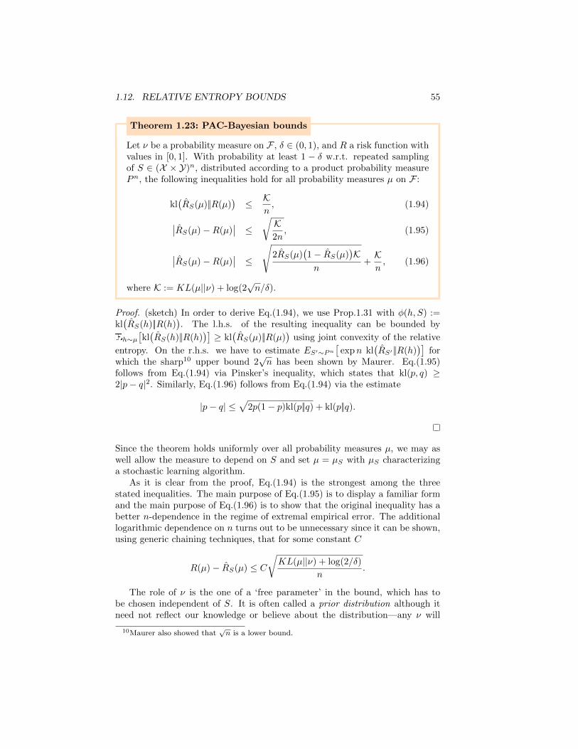
1.12. RELATIVE ENTROPY BOUNDS 55
Theorem 1.23: PAC-Bayesian bounds
Let ν be a probability measure on F , δ ∈ (0, 1), and R a risk function withvalues in [0, 1]. With probability at least 1 − δ w.r.t. repeated samplingof S ∈ (X × Y)n, distributed according to a product probability measurePn, the following inequalities hold for all probability measures µ on F :
kl(RS(µ)||R(µ)
)≤ K
n, (1.94)
∣∣RS(µ)−R(µ)∣∣ ≤
√K2n, (1.95)
∣∣RS(µ)−R(µ)∣∣ ≤
√2RS(µ)
(1− RS(µ)
)K
n+Kn, (1.96)
where K := KL(µ||ν) + log(2√n/δ).
Proof. (sketch) In order to derive Eq.(1.94), we use Prop.1.31 with φ(h, S) :=kl(RS(h)||R(h)
). The l.h.s. of the resulting inequality can be bounded by
Eh∼µ[kl(RS(h)||R(h)
)]≥ kl
(RS(µ)||R(µ)
)using joint convexity of the relative
entropy. On the r.h.s. we have to estimate ES′∼Pn[
expn kl(RS′ ||R(h)
)]for
which the sharp10 upper bound 2√n has been shown by Maurer. Eq.(1.95)
follows from Eq.(1.94) via Pinsker’s inequality, which states that kl(p, q) ≥2|p− q|2. Similarly, Eq.(1.96) follows from Eq.(1.94) via the estimate
|p− q| ≤√
2p(1− p)kl(p||q) + kl(p||q).
Since the theorem holds uniformly over all probability measures µ, we may aswell allow the measure to depend on S and set µ = µS with µS characterizinga stochastic learning algorithm.
As it is clear from the proof, Eq.(1.94) is the strongest among the threestated inequalities. The main purpose of Eq.(1.95) is to display a familiar formand the main purpose of Eq.(1.96) is to show that the original inequality has abetter n-dependence in the regime of extremal empirical error. The additionallogarithmic dependence on n turns out to be unnecessary since it can be shown,using generic chaining techniques, that for some constant C
R(µ)− RS(µ) ≤ C√KL(µ||ν) + log(2/δ)
n.
The role of ν is the one of a ‘free parameter’ in the bound, which has tobe chosen independent of S. It is often called a prior distribution although itneed not reflect our knowledge or believe about the distribution—any ν will
10Maurer also showed that√n is a lower bound.
56 CHAPTER 1. LEARNING THEORY
lead to a valid bound. Consider the simple case of a countable set F and adeterministic algorithm leading to a hypothesis h. If ν assigns a probabilityp(h) to the hypotheses, then KL(µ||ν) = log
(1/p(h)
). Hence, we essentially
recover Thm.1.5.So which prior ν should we choose? A smaller relative entropy term means
a better bound. We cannot make KL(µS ||ν) vanish though since ν must notdepend on S precluding ν = µS . However, ν is allowed to depend on n aswell as on the distribution P from which the training data is drawn. AlthoughP is unknown, we may obtain insightful bounds and/or be able to bound theresulting term in a P -independent way. In the light of this, it seems reasonableto choose ν so that KL(µS ||ν) is minimized in expectation:
Lemma 1.32 (Optimal prior distribution). For any (not necessarily product)distribution of S we obtain
argminνES[KL(µS ||ν)
]= ES [µS ], (1.97)
if the minimum is taken over all probability measures ν.
Proof. This follows from considering the difference
ES
[KL(µS ||ν)
]−KL
(ES [µS ]||ν
)= H
(ES [µS ]
)−ES
[H(µS)
].
Whatever the r.h.s. is11, the crucial point is that this difference is independentof ν. Hence, the measure ν that minimizes KL
(ES [µS ]||ν
)must also minimize
ES
[KL(µS ||ν)
]. From the properties of the relative entropy we know, however,
that the former is minimized (to zero) for ν = ES [µS ].
If we insert the optimal prior into the expected relative entropy, we obtain themutual information between the samples S and the hypotheses h. In general, iftwo random variables X and Y are governed by a joint distribution PXY whosemarginals are PX and PY , then their mutual information is defined as
I(X : Y ) := KL(PXY ||PX × PY
), (1.98)
i.e., the KL-divergence of PXY from the product of its marginals. The mutualinformation quantifies correlations between random variables, it is symmetric inits arguments, non-negative and zero iff the random variables are independent.
Lemma 1.33. ES[KL(µS ||ES′ [µS′ ])
]= I(h : S), where S′ denotes an inde-
pendent copy of S.
Proof. The learning algorithm, described by µS , together with the distributionof S defines a probability distribution on the product space F × (X × Y)n.Let us denote by p(h, S) a corresponding probability density w.r.t. a suitable
11It is the difference of two differential entropies that are defined relative to a suitablereference measure.
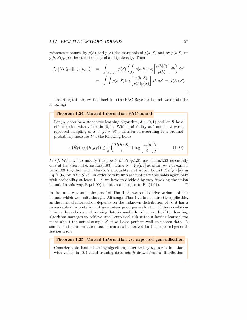
1.12. RELATIVE ENTROPY BOUNDS 57
reference measure, by p(h) and p(S) the marginals of p(h, S) and by p(h|S) :=p(h, S)/p(S) the conditional probability density. Then
ES
[KL(µS ||ES′ [µS′ ])
]=
∫
(X×Y)np(S)
(∫
Fp(h|S) log
[p(h|S)
p(h)
]dh
)dS
=
∫ ∫p(h, S) log
[p(h, S)
p(h)p(S)
]dh dS = I(h : S).
Inserting this observation back into the PAC-Bayesian bound, we obtain thefollowing:
Theorem 1.24: Mutual Information PAC-bound
Let µS describe a stochastic learning algorithm, δ ∈ (0, 1) and let R be arisk function with values in [0, 1]. With probability at least 1 − δ w.r.t.repeated sampling of S ∈ (X × Y)n, distributed according to a productprobability measure Pn, the following holds
kl(RS(µS)||R(µS)
)≤ 1
n
(2I(h : S)
δ+ log
[4√n
δ
]). (1.99)
Proof. We have to modify the proofs of Prop.1.31 and Thm.1.23 essentiallyonly at the step following Eq.(1.93). Using ν = ES [µS ] as prior, we can exploitLem.1.33 together with Markov’s inequality and upper bound KL(µS ||ν) inEq.(1.93) by I(h : S)/δ. In order to take into account that this holds again onlywith probability at least 1− δ, we have to divide δ by two, invoking the unionbound. In this way, Eq.(1.99) is obtain analogous to Eq.(1.94).
In the same way as in the proof of Thm.1.23, we could derive variants of thisbound, which we omit, though. Although Thm.1.24 is not directly applicable,as the mutual information depends on the unknown distribution of S, it has aremarkable interpretation: it guarantees good generalization if the correlationbetween hypotheses and training data is small. In other words, if the learningalgorithm manages to achieve small empirical risk without having learned toomuch about the actual sample S, it will also perform well on unseen data. Asimilar mutual information bound can also be derived for the expected general-ization error:
Theorem 1.25: Mutual Information vs. expected generalization
Consider a stochastic learning algorithm, described by µS , a risk functionwith values in [0, 1], and training data sets S drawn from a distribution
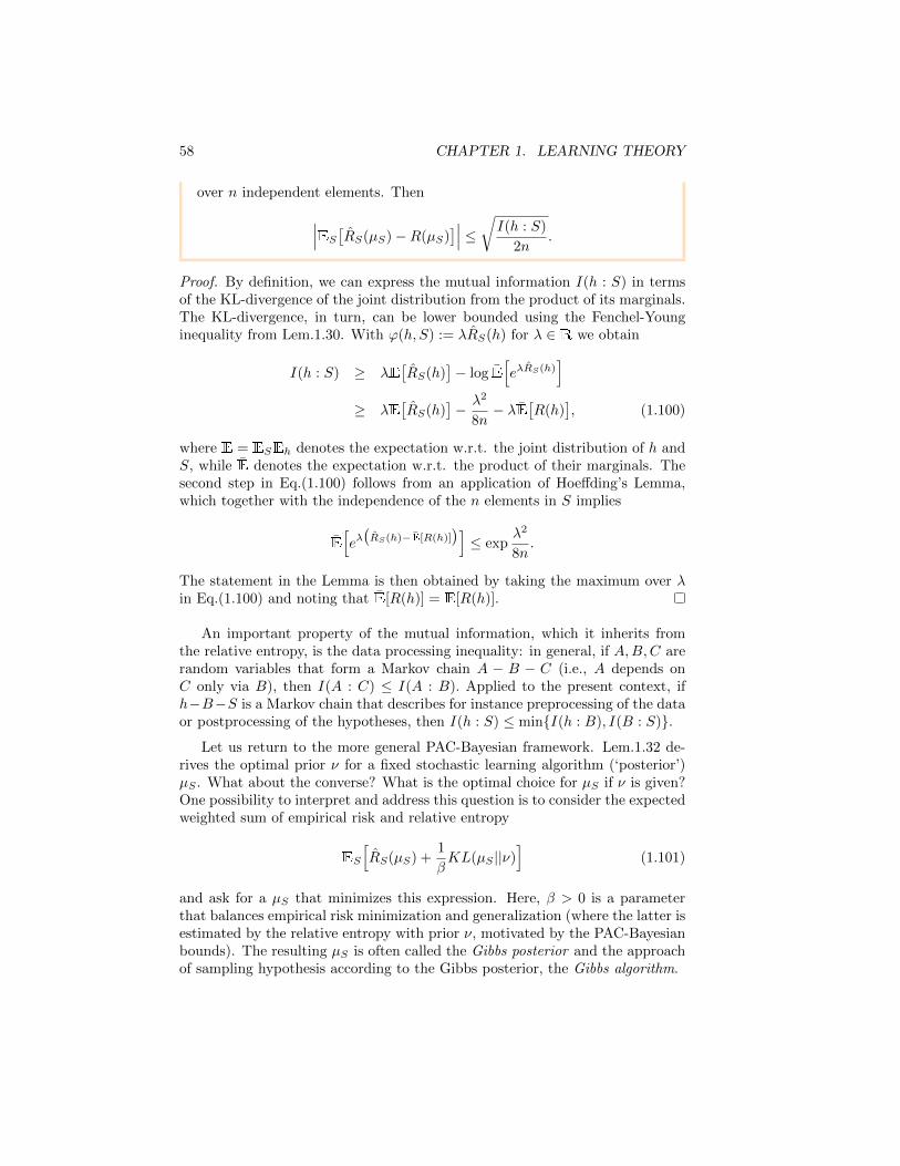
58 CHAPTER 1. LEARNING THEORY
over n independent elements. Then
∣∣∣ES[RS(µS)−R(µS)
]∣∣∣ ≤√I(h : S)
2n.
Proof. By definition, we can express the mutual information I(h : S) in termsof the KL-divergence of the joint distribution from the product of its marginals.The KL-divergence, in turn, can be lower bounded using the Fenchel-Younginequality from Lem.1.30. With ϕ(h, S) := λRS(h) for λ ∈ R we obtain
I(h : S) ≥ λE[RS(h)
]− log E
[eλRS(h)
]
≥ λE[RS(h)
]− λ2
8n− λE
[R(h)
], (1.100)
where E = ESEh denotes the expectation w.r.t. the joint distribution of h andS, while E denotes the expectation w.r.t. the product of their marginals. Thesecond step in Eq.(1.100) follows from an application of Hoeffding’s Lemma,which together with the independence of the n elements in S implies
E
[eλ(RS(h)−E[R(h)]
)]≤ exp
λ2
8n.
The statement in the Lemma is then obtained by taking the maximum over λin Eq.(1.100) and noting that E[R(h)] = E[R(h)].
An important property of the mutual information, which it inherits fromthe relative entropy, is the data processing inequality: in general, if A,B,C arerandom variables that form a Markov chain A − B − C (i.e., A depends onC only via B), then I(A : C) ≤ I(A : B). Applied to the present context, ifh−B−S is a Markov chain that describes for instance preprocessing of the dataor postprocessing of the hypotheses, then I(h : S) ≤ minI(h : B), I(B : S).
Let us return to the more general PAC-Bayesian framework. Lem.1.32 de-rives the optimal prior ν for a fixed stochastic learning algorithm (‘posterior’)µS . What about the converse? What is the optimal choice for µS if ν is given?One possibility to interpret and address this question is to consider the expectedweighted sum of empirical risk and relative entropy
ES
[RS(µS) +
1
βKL(µS ||ν)
](1.101)
and ask for a µS that minimizes this expression. Here, β > 0 is a parameterthat balances empirical risk minimization and generalization (where the latter isestimated by the relative entropy with prior ν, motivated by the PAC-Bayesianbounds). The resulting µS is often called the Gibbs posterior and the approachof sampling hypothesis according to the Gibbs posterior, the Gibbs algorithm.
1.12. RELATIVE ENTROPY BOUNDS 59
Proposition 1.34 (Optimal posterior). For given β and ν, Eq.(1.101) is min-imized for all (not necessarily product) distributions of S if µS is chosen as
dµSdν
(h) =e−βRS(h)
Eh′∼ν[e−βRS(h′)
] .
Proof. This is an immediate consequence of the Fenchel-Young inequality forthe relative entropy. Applying Lem.1.30 and setting ϕ(h) = −βRS(h) we obtain
ES
[RS(µS) +
1
βKL(µS ||ν)
]≥ ES
[Eh∼µS
[RS(h) +
1
βϕ(h)
]− 1
βlog
∫eϕdν
]
= − 1
βES
[log
∫e−βRSdν
].
Since this lower bound does not longer depend on µS , we can exploit the con-ditions for equality in Lem.1.30 and arrive at the stated result.
Note that the Gibbs algorithm can be regarded as a stochastic version ofempirical risk minimization, to which it converges in the limit β →∞.
Now it is tempting to combine the optimal posterior in Prop.1.34 with theoptimal prior from Lem.1.32 or even to see-saw these optimizations. Unfortu-nately, the optimal prior turns out to be difficult to combine with the Gibbsposterior. The analysis becomes feasible, however, for the following pair of pos-terior and prior distribution, which is motivated by the above discussion. Wedefine µS and ν in terms of probability densities pS and q w.r.t. the samesuitable reference measure12 as
pS(h) :=e−βRS(h)
Zp, q(h) :=
e−βR(h)
Zq, (1.102)
where Zp and Zq are normalization factors, defined by their purpose to let pSand q become probability densities.
Theorem 1.26: Generalization bounds for Gibbs algorithms
Let µS and ν be given by Eq.(1.102) for some β > 0, and δ ∈ (0, 1). Withprobability at least 1− δ w.r.t. repeated sampling of S ∈ (X × Y)n froman i.i.d. distribution, the following two inequalities hold simultaneously
kl(RS(µS)
)||R(µS
)≤ 1
n
(KL(µS ||ν) + log
[2√n/δ]), (1.103)
KL(µS ||ν
)≤ β2
2n+ β
√2
nlog
2√n
δ. (1.104)
12Since we are interested in their relative entropy, the reference measure will drop out inthe end.
60 CHAPTER 1. LEARNING THEORY
Moreover, I(h : S) ≤ minβ, β2/(2n)
, and
0 ≤ ES[R(µS)− RS(µS)
]≤ β
2n. (1.105)
Proof. The first inequality is just Eq.(1.94). In order to arrive at the secondinequality, observe that
KL(µS ||ν
)= Eh∼µS log
Zq e−βRS(h)
Zp e−βR(h)
= β Eh∼µS[R(h)− RS(h)
]− log
ZpZq
= β Eh∼µS[R(h)− RS(h)
]− log
∫q(h) eβ
(R(h)−RS(h)
)dh
≤ β(Eh∼µS −Eh∼ν
)[R(h)− RS(h)
], (1.106)
where we used Z−1q = q(h)eβR(h) in the third line and concavity of the log in the
last line. Eq.(1.106) implies that an upper bound on KL(µS ||ν
)can be derived
by upper and lower bounding the expectation of R(h) − RS(h) w.r.t. µS andν, respectively. Both bounds can be obtained from Eq.(1.95) when applied toµ = µS and µ = ν, respectively. Inserting these bounds into Eq.(1.106) we get
KL(µS ||ν
)≤ β√
2n
(√KL
(µS ||ν
)+ log
(2√n/δ)
+√
log(2√n/δ))
.
The largest value of KL(µS ||ν
)that is consistent with this inequality is obtained
by assuming equality and solving the resulting quadratic equation. This leadsto Eq.(1.104).
In order to obtain the claimed bound on the mutual information, we use thatcombining Lem.1.32 with Lem.1.33 leads to I(h : S) ≤ ES
[KL(µS ||ν)
]. This
holds for an arbitrary probability measure ν and if we choose ν as assumed inthe statement of the theorem, we can further bound KL(µS ||ν) via Eq.(1.106).In this way, we obtain
I(h : S) ≤ β ES[R(µS)− RS(µS)
]. (1.107)
Note that the expectation values w.r.t. ν disappeared, due to ES . FromEq.(1.107) we can obtain the stated bound on the mutual information by, onthe one hand, upper bounding the r.h.s. by β, and on the other hand, upperbounding it using Thm.1.25 and solving the resulting quadratic equation. Thelatter then leads to I(h : S) ≤ β2/(2n). Reinserting this into Thm.1.25 finallyleads to Eq.(1.105).
1.13 Differential privacy
... to be written ...
1.14. ENSEMBLE METHODS 61
1.14 Ensemble methods
Ensemble methods are meta-algorithms that combine several machine learningalgorithms or predictors to form a more powerful one. A famous example forthe success of ensemble methods is the winner of the $1M Netflix prize in 2009,which substantially improved Netflix’ recommender system. All the top sub-missions in that competition were combinations of combinations of ... hundredsof predictors. The name of one of the two teams that performed best was “TheEnsemble”.
The common idea behind all ensemble methods is to train many learningalgorithms, so-called base learners on (parts of) the training data and eventuallycombine them, for instance by averaging the resulting hypotheses or, in thecase of classification, by combining them by means of a majority vote. Thebase learners are often chosen to be relatively simple objects. Their trainingcan be done either in parallel or sequentially. This distinction can be seen asa first coarse classification of ensemble methods. Parallel schemes usually usedifferent (possibly overlapping) subsets of the training data for the differentbase learners. This reduces dependencies between the resulting hypotheses sothat averaging them has the tendency of reducing the variance and increasingstability. Sequential schemes, on the other hand, usually use the entire trainingdata set for every base learner and the training of each of them is adapted tothe performance of its successors. This usually increases the expressivity ofthe hypotheses class, decreases the bias but also the stability of the resultinglearning algorithm.
We will briefly discuss Bagging as paradigm for a parallel ensemble schemeand consider AdaBoost as well as the more general gradient boosting frameworkas examples for sequential ensemble schemes.
Bagging
Bagging stands for Bootstrap AGGregatING, which already points out the twomain ingredients of the scheme: ‘bootstrapping’ of the training data for thetraining of base learners that are eventually ‘aggregated’. Bootstrap samplingis a simple resampling technique that produces a data set B by sampling withreplacement from the training data set S. Often B is chosen to be of the samesize as S. So if |S| = |B| = n and each element in S is chosen with probability1/n, then the probability for a data point z ∈ S to be not contained in Bis (1 − 1/n)n ' 1/e ' 0.37. The idea is now to produce many such bootstrapsamples from S and to run a learning algorithm that yields a hypothesis hB ∈ Fupon input of any such B. Eventually, the resulting hypotheses are combined.In the case of regression we may just take the average. To get an intuition for theperformance of the resulting hypothesis, which is then an element of span[F ] ⊆YX , define H := EB [hB ] the expected hypothesis obtained in this way, wherethe expectation value is taken w.r.t. the bootstrap samples B.
62 CHAPTER 1. LEARNING THEORY
Theorem 1.27: L2-risk for averaged hypotheses
Consider B as a random variable to which a hypothesis hB : X → Y = R is
assigned. Define H := EB [hB ] and Var[hB(x)] := EB
[(hB(x)−H(x)
)2].
The L2-risk R (a.k.a. mean squared error) then satisfies
R(H) = EB
[R(hB)
]−EX
[Var[hB(X)]
]. (1.108)
Proof. We can express the difference between the average risk and the risk ofthe average as
EB
[R(hB)
]−R(H) = EBEX
[(hB(X)− r(X)
)2]−EX[(H(X)− r(X)
)2]
= EX
[EB
[(hB(X)
)2]−H(X)2]
= EX
[Var[hB(X)]
],
where the first equality exploited the representation of the L2-risk in terms ofthe regression function r from Thm.1.1.
Hence, if the base hypotheses hB vary significantly with B, i.e.Var[hB(x)] tendsto be large, for instance if the underlying learning algorithm is not very stable,then we can expect that averaging improves the performance—compared to theaverage performance of the base learners. On the other hand, if (possibly due tolarge overlap in the chosen data samples and stability of the chosen algorithm),the base hypotheses all perform very similar, then Bagging is not of much help.Consequently, in practice, Bagging is typically used for classes of base learnersthat tend to be not very stable. Decision trees are a typical example whereBagging, or variants thereof, improve results significantly.
AdaBoost
One of the most popular ensemble methods for binary classification is AdaBoost(short for Adaptive Boost ing). The basis of AdaBoost is a fixed hypothesesclass F ⊆ −1, 1X whose elements we call base hypotheses. AdaBoost is asequential, iterative method that when stopped after the T ’th iteration returnsa hypothesis of the form
f := sgn
(T∑
t=1
wtht
), wt ∈ R, ht ∈ F . (1.109)
That is, f is constructed so that its prediction is a weighted majority vote ofthe predictions of T base hypotheses. Note that f 6∈ F , unless F is incidentallyclosed under such operations. In every iteration of AdaBoost an ERM algorithmfor F is called as a subroutine, which returns one of the ht’s. The key idea isthat the empirical risk that is minimized within this subroutine assigns differentweights to the training data instances. The algorithm puts more weight on thoseinstances that appear to be hard in the sense that they were misclassified by
1.14. ENSEMBLE METHODS 63
the previous ht’s. Suppose the training data S consists of n pairs (xi, yi) ∈X ×−1, 1. Let p(t) be a yet to be constructed probability distribution over Sthat is used in the t’th iteration. Define by
εt :=
n∑
i=1
p(t)i 1ht(xi)6=yi (1.110)
the p(t)-weighted empirical risk of ht, i.e., the error probability of ht on S whenthe entries in S are weighted according to p(t). Given p(t), the hypothesisht is ideally chosen so that it minimizes this weighted empirical risk. We will,however, treat the selection of ht as a black box and do not require that ht reallyminimizes the weighted risk. εt is simply defined as in Eq.(1.110), whether thisis optimal or not. From here define
wt :=1
2ln
(1− εtεt
). (1.111)
The details of this choice will become clear later. For now, observe that wtincreases with decreasing εt and that wt ≥ 0 whenever εt ≤ 1
2 , i.e., wheneverthe hypothesis ht performs at least as good as random guessing. The updaterule for the probability distribution then reads
p(t+1)i :=
p(t)i
Zt×
e−wt if ht(xi) = yi
ewt if ht(xi) 6= yi
= p(t)i e−wtyiht(xi)/Zt,
where Zt is a normalization factor chosen so that∑ni=1 p
(t+1)i = 1. Note that
the step from p(t) to p(t+1) aims at increasing the weight that corresponds to(xi, yi) if xi has been misclassified by ht (in case ht performs better than randomguessing).
Upon input of the training data S, AdaBoost starts with a uniform distri-bution p(1) and iterates the above procedure, where in each iteration εt, wt, htand p(t+1) are computed. The number T of iterations is a free parameter whichessentially allows to balance between the estimation error and the approxima-tion error. If the class F of base hypotheses is simple, then small T may lead tolarge approximation error, whereas choosing T very large makes it more likelythat overly complex hypotheses are returned.
The following theorem shows that the empirical risk can decrease rapidlywith increasing T :
Theorem 1.28: Empirical risk bound for AdaBoost
Let f be the hypothesis that is returned after T iterations of AdaBoostthat led to intermediate weighted empirical risks ε ∈ [0, 1]T . Then the
64 CHAPTER 1. LEARNING THEORY
error probability of f on the training data set is bounded by
R(f) ≤T∏
t=1
2√εt(1− εt). (1.112)
With γ := min|εt−1/2|Tt=1 this implies in particular R(f) ≤ exp[−2γ2T ].
Proof. Define F :=∑Tt=1 wtht and observe that with p
(1)i = 1/n we can write
p(T+1)i = p
(1)i ×
e−w1yih1(xi)
Z1× · · · × e−wT yihT (xi)
ZT
=e−yiF (xi)
n∏Tt=1 Zt
. (1.113)
If f(xi) 6= yi, then yiF (xi) ≤ 0, which implies e−yiF (xi) ≥ 1. Therefore,
R(f) =1
n
n∑
i=1
1f(xi) 6=yi ≤1
n
n∑
i=1
e−yiF (xi) =
T∏
t=1
Zt, (1.114)
where the last step uses Eq.(1.113) together with the fact that the p(T+1)i ’s sum
up to 1. Next, we write the normalization factors Zt in a more suitable form:
Zt =
n∑
i=1
p(t)i e−wtyiht(xi) =
∑
i:ht(xi)6=yi
p(t)i ewt +
∑
i:ht(xi)=yi
p(t)i e−wt
= εtewt + (1− εt)e−wt = 2
√εt(1− εt), (1.115)
where we have inserted wt from Eq.(1.111). This completes the proof of Eq.(1.112).In order to arrive at the second claim of the theorem, we use that 1− x ≤ e−x
holds for all x ∈ R, which allows us to bound
2√εt(1− εt) =
√1− 4(εt − 1/2)2 ≤ exp
[− 2(εt − 1/2)2
].
The proof reveals two more things about AdaBoost. First, we can under-stand the particular choice of the wt’s. Looking at Eq.(1.115) one is temptedto choose them so that they minimize the expression εte
wt + (1− εt)e−wt and,indeed, this is exactly what the choice in Eq.(1.111) does. Second, notice thatafter inserting all expressions we obtain
∑
i:ht(xi)=yi
p(t+1)i =
∑
i:ht(xi)=yi
p(t)i
Zte−wt = (1− εt)
e−wt
Zt=
1
2.
This means that in every iteration the new probability distribution p(t+1) ischosen so that the correctly classified instances all together get total weight one
1.14. ENSEMBLE METHODS 65
half (and so do the misclassified ones). Hence, p(t+1) can be computed from p(t)
by a simple rescaling of the probabilities of these two sets.Thm.1.28 shows that if we manage to keep the error probabilities εt a con-
stant γ away from 1/2 (the performance of flipping a coin), the empirical riskwill decrease exponentially in the number T of iterations. More precisely, it isupper bounded by a decreasing exponential—it does in fact not have to decreasemonotonically itself.
In order to get a theoretical bound on the risk, i.e., on the performancebeyond the training data, we look at the VC-dimension:
Theorem 1.29: VC-dimension of linearly combined classifiers
Let d be the VC-dimension of F ⊆ −1, 1X and for T ∈ N define FT :=
f = sgn∑Tt=1 wtht | wt ∈ R, ht ∈ F. Then the growth function Γ of
FT satisfies
Γ(n) ≤(enT
)T (end
)Tdand (1.116)
VCdim(FT ) ≤ 2T (d+ 1) log2
(2eT (d+ 1)
). (1.117)
Proof. In order to bound the growth function we regard FT = G H as acomposition of two function classes
G :=g : RT → −1, 1
∣∣ g(z) = sgn
T∑
i=1
wizi, wi ∈ R,
H :=h : X → R
T∣∣ h(x) =
(h1(x), . . . , hT (x)
), ht ∈ F
.
Following Lemma 1.4 we have Γ(n) ≤ ΓG(n)ΓH(n) where ΓG and ΓH denotethe growth functions of G and H, respectively. Since the VC-dimension of G isequal to T by Thm.1.9, we can apply Thm.1.8 and obtain ΓG(n) ≤ (en/T )T .The product structure of H implies that ΓH(n) = ΓF (n)T where ΓF denotesthe growth function of F . The latter can by Thm.1.8 be bounded in terms ofthe VC-dimension so that ΓF (n) ≤ (en/d)d. Collecting the terms this finallyleads to Eq.(1.116).
In order to arrive at a bound for the VC-dimension, note thatD ≥ VCdim(FT )if 2D > Γ(D). Inserting the upper bound on the growth function from Eq.(1.116)this is implied by
D > T (d+ 1) log2(eD)− T log2 T − dT log2 d.
Straight forward calculation shows that this is satisfied, if we choose D equal tothe r.h.s. of Eq.(1.117).
Comparing the scaling of this bound for the VC-dimension with the one of theempirical risk in Thm.1.28 is already promising: while the VC-dimension grows
66 CHAPTER 1. LEARNING THEORY
not much faster than linearly with T , the empirical risk ideally decreases expo-nentially. In practice, AdaBoost has been observed to be remarkably resistantagainst overfitting as long as the data is not too noisy.
From a purely theoretical perspective, AdaBoost shows that a priori differ-ent notions of learnability coincide. Consider a weak and a strong notion oflearnability, where the strong notion is the one we discussed in the context ofPAC learnability. This requires a certain predicate to be true for all ε ∈ (0, 1]where the weak notion would only ask for ε ∈ (1/2−γ, 1] for some fixed, possiblysmall γ > 0. Then AdaBoost can be used to ‘boost’ learnability from weak tostrong and to show that these two notions actually coincide.
Gradient boosting
At first glance, AdaBoost may seem somewhat mysterious. One way that mightshed some light on the mystery is to view AdaBoost as part of a larger family ofsequential ensemble methods that run under the name gradient boosting. Thebasic idea behind those methods is to sequentially build up a linear combinationof base hypotheses by following gradient descent steps in function space. Here,the function whose gradient is considered is the empirical risk (or a suitablesmooth and/or convex upper bound to it). In this way, the performance on thetraining data is improved step-by-step.
In order to formalize this idea, let us fix a class F ⊆ RX of base hypothesesand define a positive, symmetric bilinear form 〈f, g〉µ := 1
n
∑ni=1 f(xi)g(xi) for
f, g ∈ span[F ]. Here, µ indicates the ‘empirical measure’ that is determined bythe points x1, . . . , xn appearing in the training data. When restricted to thelatter, we can now regard every element of span[F ] as an element of the innerproduct space L2(µ), which in tern can be identified with Rn via f(xi) =: fi.In this way, we can also regard the empirical risk as a function R : L2(µ)→ R.Starting from a base hypothesis h, it is in the light of empirical risk minimizationnow tempting to continue with an improved hypothesis of the form
h− α∇R(h), (1.118)
i.e., to move with a suitably chosen step-size α > 0 in the direction of steepestdescent w.r.t. R. This direction is given by the negative gradient of R. If thestep in Eq.(1.118) can be made to work, it can be iterated yielding a sequen-tially growing linear combination of hypotheses with decreasing empirical risk.Assuming that the loss function is differentiable in its second argument we canexpress the i-th component of the gradient as
(∇R(h)
)i
= ∂2L(yi, h(xi)
). (1.119)
Before continuing with the general discussion, let us look at an instructiveexample and consider the quadratic loss L(y, y′) := (y − y′)2/2 for which∇R(h)i = h(xi) − yi. Inserting this with α = 1 into Eq.(1.118) exhibits someclosely related issues that have to be resolved before the underlying idea canwork: (i) already after the first step the resulting hypothesis h − ∇R(h) has
1.14. ENSEMBLE METHODS 67
zero empirical risk, suggesting that the method is prone to overfitting; (ii) asan element of L2(µ) the gradient is only defined for x ∈ x1, . . . , xn; (iii) thereis no general reason for the gradient to be realizable within F .
For these reasons, instead of choosing the gradient itself, one uses an approx-imation of the gradient within F . This can be done for instance by choosing ag ∈ F that maximizes the overlap with the negative gradient in the sense thatideally
g := argmaxf∈F−〈∇R(ht), f〉µ√
〈f, f〉µ. (1.120)
From now on assume that F ⊆ −1, 1X , which implies that 〈f, f〉µ = 1 forany f ∈ F . Moreover, we restrict the discussion to loss functions of the formL(y, y′) := φ(yy′) with φ : R → R decreasing and differentiable (or convex inwhich case a subderivative can be used in stead of the derivative). Commonexamples are φ(z) = e−z, giving rise to the exponential loss, φ(z) = max1 −z, 0, leading to the hinge loss, or φ(z) = log2(1 + e−z) yielding the logit loss.Note that these are all convex upper bounds on the 0-1-loss function in the sensethat φ(yz) ≥ 1y 6=sgn[z] for all z ∈ R and y ∈ −1, 1.
Expressing the overlap with the gradient, which appears in Eq.(1.120), interms of φ gives
〈∇R(ht), f〉µ =1
n
n∑
i=1
f(xi)yiφ′(yih(xi)
)
=1
n
n∑
i=1
φ′(yih(xi)
)(1− 21f(xi)6=yi
).
Therefore, the maximizers of Eq.(1.120) are the minimizers of a weighted em-pirical risk function of the form
ε :=
n∑
i=1
pi1f(xi)6=yi , with pi :=φ′(yih(xi))∑nj=1 φ
′(yjh(xj)).
Once a function g ∈ F that (ideally) minimizes this expression is chosen, itremains to determine the step size α. A natural way to do this is via ‘linesearch’, i.e., by minimizing R(h + αg) w.r.t. α. For the exponential loss thisminimization can be done analytically and, after few elementary steps, leadsprecisely to the expression found in AdaBoost, namely
α =1
2ln
1− εε
.

68 CHAPTER 1. LEARNING THEORY
Chapter 2
Neural networks
2.1 Information processing in the brain
The human brain contains about 1011 neurons, which can be regarded as itsbasic information processing units. A typical neuron consist of a cell body,dendrites, which receive incoming signals from other neurons and an axon, whichtransmits signals to other neurons. While there are typically several dendritesoriginating from the cell body and then branching out in the neighborhood ofthe neuron, there is only one axon, which may have a local branching in theneighborhood of the cell body and a second branching at a distance. This canmean everything from 0.1mm to 2m.
On the macroscopic scale, if we regard the human brain as a whole, we seeit covered with a folded outer layer, which is about 3mm thick (when unfolded),and called the cerebral cortex. The largest part of the cerebral cortex is also itsevolutionary youngest part and for this reason called neocortex. The neocortexplays a crucial role in many higher brain functions.
If we look at slices of the brain, we see the cerebral cortex as gray matterclearly separated from the white matter, which it surrounds. White matteralmost exclusively consists of axons that connect more distant parts of thebrain. The axons originate from neurons (mainly so-called pyramidal neurons,named after their shape), which are part of the gray matter, then leave thegray matter, traverse parts of the brain in the white matter, which is formedby them, and then reenter the gray matter and connect to other neurons. Inthis sense, white matter is related to (long distance) communication, whereasinformation storage and processing happens in the gray matter. The differencein color stems from the myelin, a fatty white substance which covers the axonsin the white matter. The main purpose of the myelin sheaths is to increase thespeed at which signals travel down the axons. Therefore, only the long distanceconnections are covered with myelin.
The gray matter exhibits horizontal as well as vertical substructures. In mostregions, six horizontal layers can be identified that distinguished depending on
69
70 CHAPTER 2. NEURAL NETWORKS
the occurring neuronal cell types and/or the types of connections with otherregions.1 There are also vertical units, called cortical (mini)collumns, whichare sometimes regarded as the basic functional units (or elementary patternrecognizers) in the brain. However, depending on the region of the brain, thisviewpoint is subject of debate.
A typical pyramidal neuron in the neocortex forms a highly connected localnetwork in the gray matter where it is connected to about 104 of its neigh-bors that are less then 1mm apart. In addition, via the axon traversing thewhite matter, the neuron is connected to a similar number of distant neurons.There is evidence that connections between different regions of the neocortexare typically two-way connections in the sense of region-to-region, but usuallynot point-to-point.
The neocortex is very homogeneous throughout the brain so that differentfunctions that are assigned to different areas are not obviously reflected physi-ologically. The assignment of special functions to specific areas clearly dependson which parts or sensory inputs the area is connected to.
The signals between neurons are electrical pulses that originate in a changeof the electrical potential of in total about 100mV—the action potential. Sucha pulse takes about 1ms and travels down the axon where it reaches so-calledsynapses at the axon’s branches. A synapse connects the axon of one neu-ron with the dendrite of another neuron. The signal transmission within mostsynapses is of chemical nature. The arriving electrical pulse induces a chemicalprocess inside the synapse, which in turn leads to a change of electrical potentialin the postsynaptic neuron. The time it takes for a signal to pass a chemicalsynapse is around 1ms.
In the dendritic part of the postsynaptic neuron all the incoming signalsare integrated. If they lead to a joint stimulus above a certain threshold, theywill cause an action potential and the neuron will fire. This is an all-or-nothingprocess and all stimuli above threshold lead to the same pulse with standardizedamplitude and duration. While the outgoing signal in this way can be considereddigital, the integration/accumulation of the incoming signals appears to be moreof analog nature.
The effect of an incoming pulse on the postsynaptical neuron can varysignificantly—over time, in duration and in strength. It may change the po-tential from milliseconds to minutes and during this period have an excitatoryor an inhibitory effect.2 The variability of the strength of this effect is consideredcrucial for purposes of learning and memorization.
A neuron can fire several hundred times per second (while the average firingrate is closer to 1Hz). A limiting factor to higher rates is the duration of eachpulse and a corresponding refractory period of about 1ms after initiation of anaction potential during which no stimulus can lead to firing. Within about 4msafter this strict refractory period stimuli still have to be stronger than usual to
1These layers, however, are very different from the layers we will encounter later on.2However, connections between pyramidal neurons, which are believed to correspond to
the majority of synapses in the cerebral cortex, are exclusively excitatory.
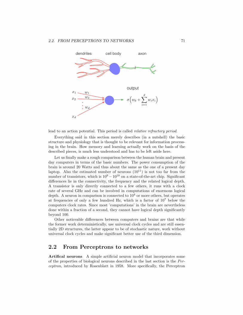
2.2. FROM PERCEPTRONS TO NETWORKS 71
dendrites cell body axon
outputx1
x2
xd
w0 +
dX
i=1
wixi
w1
w2
wd
lead to an action potential. This period is called relative refractory period.
Everything said in this section merely describes (in a nutshell) the basicstructure and physiology that is thought to be relevant for information process-ing in the brain. How memory and learning actually work on the basis of thedescribed pieces, is much less understood and has to be left aside here.
Let us finally make a rough comparison between the human brain and presentday computers in terms of the basic numbers. The power consumption of thebrain is around 20 Watts and thus about the same as the one of a present daylaptop. Also the estimated number of neurons (1011) is not too far from thenumber of transistors, which is 109− 1010 on a state-of-the-art chip. Significantdifferences lie in the connectivity, the frequency and the related logical depth.A transistor is only directly connected to a few others, it runs with a clockrate of several GHz and can be involved in computations of enormous logicaldepth. A neuron in comparison is connected to 104 or more others, but operatesat frequencies of only a few hundred Hz, which is a factor of 107 below thecomputers clock rates. Since most ’computations’ in the brain are neverthelessdone within a fraction of a second, they cannot have logical depth significantlybeyond 100.
Other noticeable differences between computers and brains are that whilethe former work deterministically, use universal clock cycles and are still essen-tially 2D structures, the latter appear to be of stochastic nature, work withoutuniversal clock cycles and make significant better use of the third dimension.
2.2 From Perceptrons to networks
Artifical neurons A simple artificial neuron model that incorporates someof the properties of biological neurons described in the last section is the Per-ceptron, introduced by Rosenblatt in 1958. More specifically, the Perceptron
72 CHAPTER 2. NEURAL NETWORKS
incorporates (i) several inputs whose effects are determined by variable weights,(ii) a single output (which may, however, be copied/fanned out an arbitrarynumber of times), (iii) integration of input signals and (iv) an all-or-nothingprocess with adjustable threshold.
Mathematically, each input is characterized by a real number xi where i =1, . . . , d runs over the number of inputs. Each of the input lines gets assigned aweight wi ∈ R. The mapping from the inputs to the output is then modeled by
x 7→ σ
(w0 +
d∑
i=1
wixi
), (2.1)
where w0 ∈ R plays the role of a threshold value and the activation functionσ : R→ R is, in the case of the Perceptron, given by the step-function σ(z) =1z≥0. It is convenient to regard w0 as the weight of a constant input x0 = 1.Nowadays, one usually considers generalizations of this model that differ fromthe original Perceptron in the choice of the activation function. The main reasonfor choosing different activation functions is that they enable gradient descenttechniques for learning algorithms. Common choices are:
• Logistic sigmoid3 σ(z) = 11+e−z ,
• Hyperbolic tangent σ(z) = tanh(z) (which is an affinely transformed logis-tic sigmoid),
• Rectified linear σ(z) = max0, z. This is sometimes modified to maxαx, xwith some α ∈ (0, 1).
Note that the logistic sigmoid function and the hyperbolic tangent are smoothversions of the step functions 1z≥0 and sgn(z), respectively. In practice, thelogistic sigmoid and tanh, which were used over many years, are nowadays moreand more replaced by rectified linear activation functions.
A multivariate function of the form Rd 3 x 7→ σ(w · x) with σ : R → R
is often called a ridge function - especially in the context of approximationtheory. Note that every ridge function is constant on hyperplanes characterizedby w · x = c. In the case of the Perceptron with σ(z) = 1z≥0 we have thatthe set of points in Rd that are mapped to 1 forms a closed half space. Thisrelation between Perceptrons and half spaces is obviously bijective and oftenprovides a useful geometric depiction. However, the simplicity of this geometryalso suggests that a single Perceptron will only be sufficiently expressive in veryfew cases. Richer function classes can be obtain from the Perceptron in at leastthree a priori different ways:
• By using Perceptrons as base hypotheses for boosting algorithms as dis-cussed in Sec.1.14.
• By first embedding the data in a larger (typically infinite-dimensional)space and applying the linear structure of the Perceptron in this larger
3”Sigmoidal” just means S-shaped.
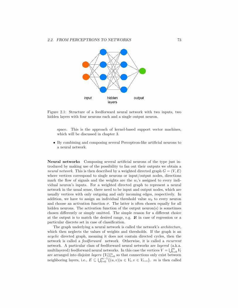
2.2. FROM PERCEPTRONS TO NETWORKS 73
Figure 2.1: Structure of a feedforward neural network with two inputs, twohidden layers with four neurons each and a single output neuron.
space. This is the approach of kernel-based support vector machines,which will be discussed in chapter 3.
• By combining and composing several Perceptron-like artificial neurons toa neural network.
Neural networks Composing several artificial neurons of the type just in-troduced by making use of the possibility to fan out their outputs we obtain aneural network. This is then described by a weighted directed graph G = (V,E)where vertices correspond to single neurons or input/output nodes, directionsmark the flow of signals and the weights are the wi’s assigned to every indi-vidual neuron’s inputs. For a weighted directed graph to represent a neuralnetwork in the usual sense, there need to be input and output nodes, which areusually vertices with only outgoing and only incoming edges, respectively. Inaddition, we have to assign an individual threshold value w0 to every neuronand choose an activation function σ. The latter is often chosen equally for allhidden neurons. The activation function of the output neuron(s) is sometimeschosen differently or simply omitted. The simple reason for a different choiceat the output is to match the desired range, e.g. R in case of regression or aparticular discrete set in case of classification.
The graph underlying a neural network is called the network’s architecture,which then neglects the values of weights and thresholds. If the graph is anacyclic directed graph, meaning it does not contain directed cycles, then thenetwork is called a feedforward network. Otherwise, it is called a recurrentnetwork. A particular class of feedforward neural networks are layered (a.k.a.multilayered) feedforward neural networks. In this case the vertices V =
⋃ml=0 Vl
are arranged into disjoint layers Vlml=0 so that connections only exist between
neighboring layers, i.e., E ⊆⋃m−1l=0 (u, v)|u ∈ Vl, v ∈ Vl+1. m is then called
74 CHAPTER 2. NEURAL NETWORKS
the depth of the network and m − 1 is the number of hidden layers (”hidden”in the sense of in between input and output). In the following we will focus onlayered feedforward networks. If there is no further specification, we will alwaysassume that neighboring layers are fully connected, i.e., every element of Vl isconnected to every element in Vl+1.
Other models Before analyzing in greater detail layered feedforward net-works, let us make one step back and have a quick look at other models thatrun (or might run) under the name ‘artificial neural network’ as well. What allthese models have in common is an underlying graph structure with the verticesof the graph playing the role of ‘artificial neurons’. That is, they are all graphi-cal models. Probably the biggest distinction is between directed and undirectedgraphs.
In models using directed graphs, the neurons can directly be seen as ‘in-formation processing units’ for which the directions of the edges specify thedirections of the information flow. Mathematically speaking, in this case oneassigns to each neuron a function from a product space corresponding to theincoming edges to the one of the outgoing edges. In principle, this could be anyfunction. In practice, however, the traditional structure of this function is anaffine mapping composed with a non-affine function σ : R→ R composed witha fan-out. Here the ‘activation function’ σ is usually fixed so that all the freeparameters of the model are contained in the affine transformations. While inthe case of recurrent networks one has to deal with time series, in the case offeedforward networks the entire network then is characterized by a single func-tion from the input to the output space. In the layered case this is thus of theform
Rd 3 x 7→ σm Am σm−1 . . . A2 σ1 A1x,
i.e., an alternation of affine maps A1, . . . , Am, which carry all free parameters,with fixed activation functions. The latter are often chosen all equal and fromR to R (then applied component-wise), but are not necessarily so. It seems thatthis structure is relaxed more and more. Nevertheless, for the largest part ofthe analysis, we will consider this ‘traditional’ structure. This also concerns theuse of deterministic functions A and σ rather than the application of stochasticmappings, which would probably be closer to the biological origin and fall intothe realm of Bayesian networks.
Models based on undirected graphs are of very different nature and willnot be discussed beyond this paragraph. The idea in this case is to assigna random variable to each vertex and to let them ‘interact’ according to thepattern specified by the graph. This leads to Markov random fields and modelsthat are well-studied in statistical physics under the names Ising-/Potts model orSpin glasses. Used as neural networks, where the parameters of the interactionsare to be learned, these models are called Boltzmann machines.
2.3. REPRESENTATION AND APPROXIMATION 75
2.3 Representation and approximation
A feedforward neural network with d inputs and d′ outputs represents a functionf : Rd → Rd
′. In this section we address the question which functions can be
represented (exactly or approximately) by a layered feedforward neural network,depending on the architecture and on the chosen activation function. We willstart with the discrete case.
Representation of Boolean functions As a warm-up, consider a singlePerceptron with two Boolean inputs. Can it represent basic Boolean functionslike AND, OR, NAND or XOR? The simple but crucial observation for answer-ing this question is that the function fw : Rd → R in Eq.(2.1) that describesa Perceptron is, for every choice of the weights w ∈ Rd+1, constant on hyper-planes that are orthogonal to the vector (w1, . . . , wd). Moreover, due to thespecial choice of σ as a step function fw separates half-spaces and by choosingsuitable weights any half-space can be separated from its complement.
If we regard the inputs of AND, OR or NAND as points in R2, then in allthree cases the subsets that are mapped to 0 or 1 can be separated from eachother by a line. Consequently, AND, OR and NAND can be represented by asingle Perceptron. This is already somewhat promising since we know that everyBoolean function can be obtained as a composition of many of such buildingblocks. XOR, on the other hand, cannot be represented by a single Perceptronsince in this case the inputs that are mapped to 0 cannot be linearly separatedfrom the ones mapped to 1. This implies that representing an arbitrary Booleanfunction by a feedforward neural network requires at least one hidden layer. Thefollowing theorem shows that a single hidden layer is already sufficient.
Theorem 2.1: Representation of Boolean functions
Every Boolean function f : 0, 1d → 0, 1 can be represented exactlyby a feedforward neural network with a single hidden layer containing atmost 2d neurons, if σ(z) = 1z≥0 is used as activation function.
Proof. If a, b ∈ 0, 1 are Boolean variables, then 2ab− a− b ≤ 0 with equality
iff a = b. With this observation we can write 1x=u = σ(∑d
i=1 2xiui − xi − ui)
for x, u ∈ 0, 1d. Denoting by A := f−1(1)
the set of all vectors u for whichf(u) = 1, we can then represent f as
f(x) = σ(− 1 +
∑
u∈A1x=u
)= σ
(− 1 +
∑
u∈Aσ( d∑
i=1
2xiui − xi − ui)), (2.2)
which is the sought representation using a single hidden layer with |A| ≤ 2d
neurons.
We will see in Sec.2.4 that the exponential increase of the number of neuronscannot be avoided.
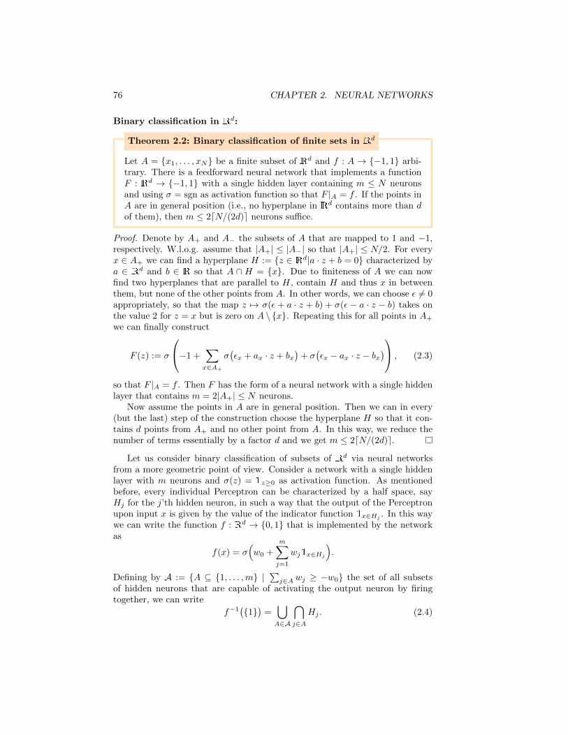
76 CHAPTER 2. NEURAL NETWORKS
Binary classification in Rd:
Theorem 2.2: Binary classification of finite sets in Rd
Let A = x1, . . . , xN be a finite subset of Rd and f : A → −1, 1 arbi-trary. There is a feedforward neural network that implements a functionF : Rd → −1, 1 with a single hidden layer containing m ≤ N neuronsand using σ = sgn as activation function so that F |A = f . If the points inA are in general position (i.e., no hyperplane in Rd contains more than dof them), then m ≤ 2dN/(2d)e neurons suffice.
Proof. Denote by A+ and A− the subsets of A that are mapped to 1 and −1,respectively. W.l.o.g. assume that |A+| ≤ |A−| so that |A+| ≤ N/2. For everyx ∈ A+ we can find a hyperplane H := z ∈ Rd|a · z + b = 0 characterized bya ∈ Rd and b ∈ R so that A ∩ H = x. Due to finiteness of A we can nowfind two hyperplanes that are parallel to H, contain H and thus x in betweenthem, but none of the other points from A. In other words, we can choose ε 6= 0appropriately, so that the map z 7→ σ(ε + a · z + b) + σ(ε − a · z − b) takes onthe value 2 for z = x but is zero on A \ x. Repeating this for all points in A+
we can finally construct
F (z) := σ
−1 +
∑
x∈A+
σ(εx + ax · z + bx
)+ σ
(εx − ax · z − bx
) , (2.3)
so that F |A = f . Then F has the form of a neural network with a single hiddenlayer that contains m = 2|A+| ≤ N neurons.
Now assume the points in A are in general position. Then we can in every(but the last) step of the construction choose the hyperplane H so that it con-tains d points from A+ and no other point from A. In this way, we reduce thenumber of terms essentially by a factor d and we get m ≤ 2dN/(2d)e.
Let us consider binary classification of subsets of Rd via neural networksfrom a more geometric point of view. Consider a network with a single hiddenlayer with m neurons and σ(z) = 1z≥0 as activation function. As mentionedbefore, every individual Perceptron can be characterized by a half space, sayHj for the j’th hidden neuron, in such a way that the output of the Perceptronupon input x is given by the value of the indicator function 1x∈Hj . In this waywe can write the function f : Rd → 0, 1 that is implemented by the networkas
f(x) = σ(w0 +
m∑
j=1
wj1x∈Hj
).
Defining by A := A ⊆ 1, . . . ,m |∑j∈A wj ≥ −w0 the set of all subsets
of hidden neurons that are capable of activating the output neuron by firingtogether, we can write
f−1(1)
=⋃
A∈A
⋂
j∈AHj . (2.4)
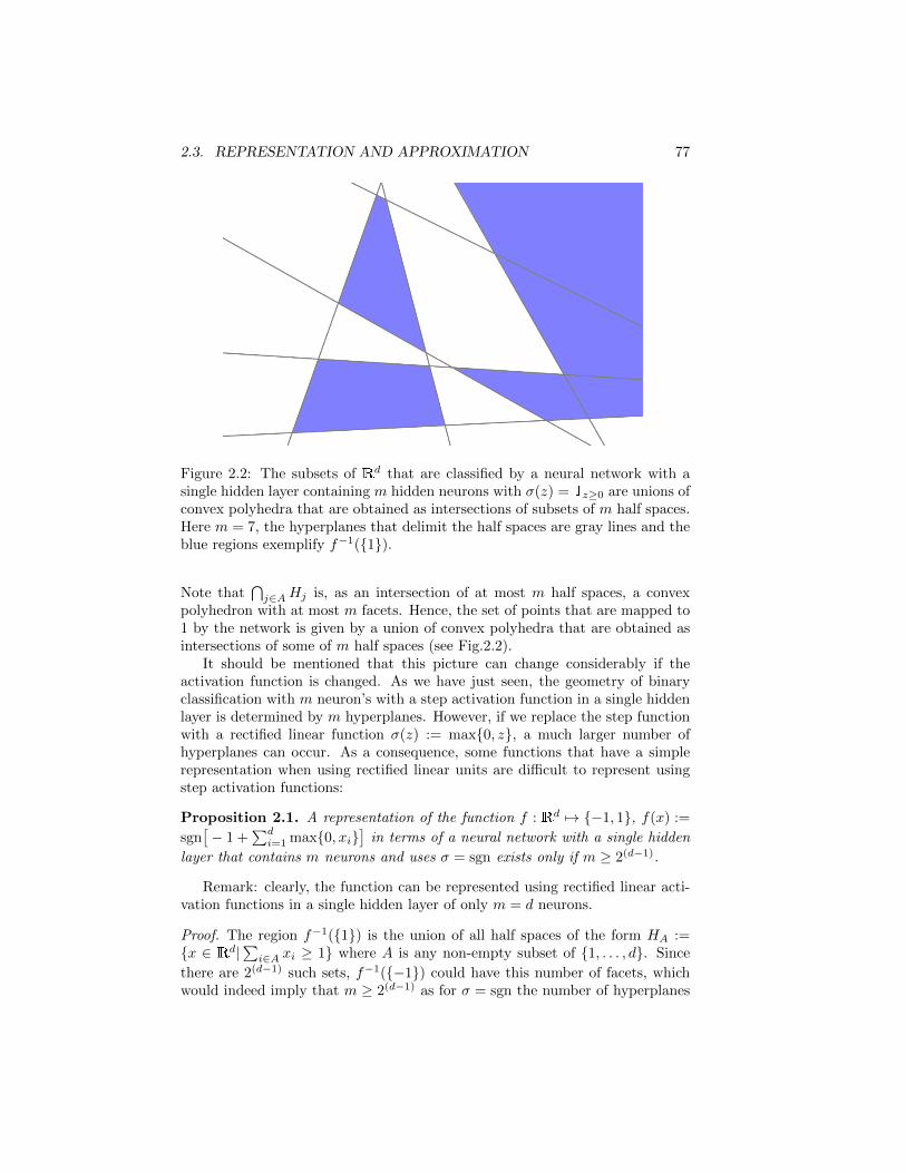
2.3. REPRESENTATION AND APPROXIMATION 77
Figure 2.2: The subsets of Rd that are classified by a neural network with asingle hidden layer containing m hidden neurons with σ(z) = 1z≥0 are unions ofconvex polyhedra that are obtained as intersections of subsets of m half spaces.Here m = 7, the hyperplanes that delimit the half spaces are gray lines and theblue regions exemplify f−1(1).
Note that⋂j∈AHj is, as an intersection of at most m half spaces, a convex
polyhedron with at most m facets. Hence, the set of points that are mapped to1 by the network is given by a union of convex polyhedra that are obtained asintersections of some of m half spaces (see Fig.2.2).
It should be mentioned that this picture can change considerably if theactivation function is changed. As we have just seen, the geometry of binaryclassification with m neuron’s with a step activation function in a single hiddenlayer is determined by m hyperplanes. However, if we replace the step functionwith a rectified linear function σ(z) := max0, z, a much larger number ofhyperplanes can occur. As a consequence, some functions that have a simplerepresentation when using rectified linear units are difficult to represent usingstep activation functions:
Proposition 2.1. A representation of the function f : Rd 7→ −1, 1, f(x) :=
sgn[− 1 +
∑di=1 max0, xi
]in terms of a neural network with a single hidden
layer that contains m neurons and uses σ = sgn exists only if m ≥ 2(d−1).
Remark: clearly, the function can be represented using rectified linear acti-vation functions in a single hidden layer of only m = d neurons.
Proof. The region f−1(1) is the union of all half spaces of the form HA :=x ∈ Rd|
∑i∈A xi ≥ 1 where A is any non-empty subset of 1, . . . , d. Since
there are 2(d−1) such sets, f−1(−1) could have this number of facets, whichwould indeed imply that m ≥ 2(d−1) as for σ = sgn the number of hyperplanes

78 CHAPTER 2. NEURAL NETWORKS
is at most the number of neurons in the hidden layer. So, it remains to showthat none of these half spaces is redundant in the characterization of f−1(−1).This is done by constructing a point x for every nonempty A ⊆ 1, . . . , d sothat x ∈ HA′ ⇒ A′ = A. A possible choice for such a point is
xi =
1|A| , i ∈ A−1 , i 6∈ A
Let us conclude the geometric discussion with a classical theorem that pro-vides a tight bound on the number of regions into which Rd is cut by n hyper-planes. For its proof we again use the relation between VC-dimension and ‘cellcounting’ that has led to Thm.1.10, but now in the opposite direction.
Theorem 2.3: Zaslavsky’s theorem
Let h1, . . . , hn ⊆ Rd be hyperplanes. The number N of connected compo-nents of Rd \
⋃ni=1 hi then satisfies
N ≤d∑
i=0
(n
i
)≤(end
)d. (2.5)
Remark: the first inequality can be shown to be tight. A generic collection ofn hyperplanes turns out to cut Rd into exactly
∑di=0
(ni
)regions.
Proof. (sketch) By translation we can always ensure that none of the consideredhyperplanes goes through the origin. Under this assumption, every hyperplanecan be characterized by a vector w ∈ Rd via h := x ∈ Rd|〈x,w〉 = 1.Denote by X the set of all these hyperplanes in Rd, and define a set of functionsF ⊆ −1, 1X via F := h 7→ sgn[g(h)] | g ∈ G, where G := h 7→ 〈x,w〉 −1 | x ∈ Rd with w being the vector characterizing h. Every function in F thencorresponds to a single point in Rd and assigns a value ±1 to a hyperplane,depending on whether the point lies on one side of the plane or on the other. AsG ' Rd forms a d-dimensional affine space (a small modification of) Thm.1.9implies that V Cdim(F) = d.
Assume now that a collection A ⊆ X of n hyperplanes separate N regionsin Rd. That is, there are N points in Rd so that for any pair of them, thereis one separating hyperplane among the n considered ones. In other words,F|A contains at least N different functions and since |A| = n this implies thatN ≤ Γ(n), where Γ denotes the growth function of F . Using Thm.1.8 wecan bound the growth function in terms of the VC-dimension, and thus d, inprecisely the way stated in Eq.(2.5).
Representing real-valued functions on finite sets Now we move to real-valued functions and first consider the case of finite domains. The following the-orem provides an example of a feedforward neural network in which the number
2.3. REPRESENTATION AND APPROXIMATION 79
of parameters required in order to exactly represent an arbitrary assignmentof real numbers to N points in Rd scales linearly with N . The network thatimplements the function involves weight sharing in the sense that the weightsof the edges between the d inputs and the neurons of the hidden layer do notdepend on the neuron.
Theorem 2.4: Representation with few parameters
Let A = x1, . . . , xN be a finite subset of Rd and f : A → R arbitrary.There is a feedforward neural network that implements a function F :Rd → R with a single hidden layer containing N neurons and 2N + dparameters so that F |A = f . The network can be chosen such that it usesthe ReLU activation function σ(x) = max0, x in the hidden layer andthe identity as activation function at the output.
Note: The additional ‘+d’ parameters depend only weakly on A and f . As willbe seen in the proof, a random choice will do the job with probability one, sothat there are really only 2N essential parameters. These correspond to theweights of the output neuron and the biases/threshold values of the neurons inthe hidden layer.
Proof. The function F : Rd → R,
F (x) :=
N∑
j=1
aj max0, w · x− vj
has 2N + d parameters given by w ∈ Rd, a, v ∈ RN and it can be implementedusing a neural network of the specified type. We have to show that there isalways a choice of parameters that solves the set of equations F (xi) = f(xi),i = 1, . . . , N . Such a solution exists, if the N × N matrix M with entriesMi,j := max0, w · xi − vj is invertible, since we can then simply choose aj :=∑iM−1j,i f(xi). W.l.o.g. we can assume that A contains N distinct elements.
Then there exists a w ∈ Rd so that all zi := w ·xi are distinct, as well. Assumingin addition that the zi’s are in increasing order (and otherwise relabeling themaccordingly) we can choose v so that v1 < z1 < v2 < z2 < . . .. In this wayM becomes a triangular matrix with non-vanishing diagonal entries and is thusinvertible.
Bounded storage capacity Thm.2.4 shows, that the number of data pointsthat can be ‘memorized’ exactly by a ReLU-based neural network scales at leastlinearly with the number of parameters. On the other hand, counting dimen-sions, one would expect that the number of data points that can be memorizedcannot exceed the number of parameters, either, irrespective of the chosen ac-tivation function. This intuition is made rigorous by the following theorem. Asin the previous theorem the number of parameters is given by the number offree weights (incl. biases), possibly reduced by weight sharing.
80 CHAPTER 2. NEURAL NETWORKS
Theorem 2.5: Maximal storage capacity
Consider a feedforward neural network that depends on M real parametersand for any given parameter vector w ∈ RM is described by a map Rd 3x 7→ F (x,w) ∈ Rd′ . Assume that (i) all activation functions are piecewisecontinuously differentiable with derivatives that are bounded on boundeddomains and (ii) there is a set of inputs x1, . . . , xN ∈ Rd such that forany y1, . . . , yN ∈ Rd
′there is a w ∈ RM for which F (xi, w) = yi ∀i ∈
1, . . . , N. Then necessarily
N ≤ M
d′. (2.6)
Proof. Consider the activation function σ : R→ R at an arbitrary node in thenetwork. Since it is, by assumption, piecewise C1 with bounded derivatives, wecan extend each branch to a C1-function defined on the entire real line and inthis way obtain a countable set of functions σα ∈ C1(R)α∈N such that forany x ∈ R there is an α so that σ(x) = σα(x). In particular,
⋃α σα(x) ⊇ σ(x)
for any x ∈ Rd. Applying this idea to each of the (finitely many) activationfunctions in the network, we can lift the argument to the entire network: thereis a countable family of functions Fα ∈ C1(Rd × RM ) with the property thatF (x,w) ⊆
⋃α Fα(x,w).
Assumption (ii) demands that the mapping Φ : RM → Rd′N , Φ(w) :=(
F (x1, w), . . . , F (xN , w))
satisfies Φ(RM ) = Rd′N . On the other hand, we can
define Φα(w) :=(Fα(x1, w), . . . , Fα(xN , w)
)and bound
⋃α Φα(RM ) ⊇ Φ(RM ).
Now suppose Nd′ > M and let µ be the Nd′-dimensional Lebesgue-measure.For the next step we use that C1-functions map sets of measure zero (like RM
as a subspace within RNd′) to sets of measure zero. Using in addition the fact
that a countable union of such sets still has measure zero we obtain
µ(Φ(RM )
)≤ µ
(⋃
α
Φα(RM )
)= 0.
Since this contradicts assumption (ii), we have to have Nd′ ≤M .
Approximating real-valued functions We will begin with the one-dimen-sional case f : R → R and later lift the obtained results to the case of higherdimensional input and output spaces. Let us denote by Fσ,m the class of func-tions representable by a feedforward network with a single hidden layer with mneurons in the hidden layer. That is,
Fσ,m :=f : R→ R
∣∣ f(x) =
m∑
v=1
avσ(wvx+ bv), av, bv, wv ∈ R
(2.7)
and define Fσ :=⋃m∈N Fσ,m. Note that there is no activation function (or,
equivalently, just the identity) at the output.
2.3. REPRESENTATION AND APPROXIMATION 81
The following approximation theorem is formulated in terms of the modulusof continuity of the function f to be approximated. It is defined as
ω(f, δ) := supx,y:|x−y|≤δ
∣∣f(x)− f(y)∣∣. (2.8)
Note that if f is uniformly continuous, then ω(f, δ) → 0 for δ → 0. Moreover,if f is L−Lipschitz, then ω(f, δ) ≤ δL.
Theorem 2.6: Approximations using bounded sigmoids
Let σ : R→ R be any bounded function that satisfies limz→−∞ σ(z) = 0and limz→∞ σ(z) = 1. There is a constant c so that for every f ∈ C
([0, 1]
)
and every m ∈ N we have
inffm∈Fσ,m
||f − fm||∞ ≤ c ω(f, 1/m). (2.9)
Note: From the proof we get that c = 2 + 2||σ||∞ is a valid constant (where||σ||∞ = supz∈R |σ(z)|). A more careful analysis shows that c = ||σ||∞ suffices.The assumption that σ is asymptotically either 0 or 1 is convenient for the proofbut not really crucial. The same argument works if only the limits limz→±∞ σ(z)exist inR and differ from each other. Similarly, the domain [0, 1] can be replacedby any compact subset of R.
Proof. The idea is to first approximate f by a piecewise constant function hmand then hm by an appropriate fm. Define xi := i/m and hm(x) so that ittakes the value f(xi) in the interval x ∈
[xi−1, xi
)where i = 1, . . . ,m. By
construction ||f − hm||∞ ≤ ω(f, 1/m). With j := bmxc write
hm(x) = f(x1) +
j∑
i=1
(f(xi+1)− f(xi)
)and define
fm(x) := f(x1)σ(α) +
m−1∑
i=1
(f(xi+1)− f(xi)
)σ(α(mx− i)
), (2.10)
for some α ∈ R to be chosen shortly. Note that fm is of the desired form.The claim is that fm approximates hm well for large α. To bound the distancebetween the two functions, fix any ε > 0 and choose α such that |σ(z)−1z≥0| ≤ε/m whenever |z| ≥ α. This is possible since σ is assumed to be a sigmoidalfunction. Note that, by the choice of α, we get that if i 6∈ j, j + 1 the termσ(α(mx− i)
)is ε/m-close to the step function 1i≤bmxc. Consequently, we can
bound
|fm(x)− hm(x)| ≤ ε
m
[|f(x1)|+ (m− 2)ω(f, 1/m)
]
+∣∣f(xj+1)− f(xj)
∣∣∣∣∣1− σ
(α(mx− j)
)∣∣∣
+∣∣f(xj+2)− f(xj+1)
∣∣∣∣∣σ(α(mx− j − 1)
)∣∣∣,
82 CHAPTER 2. NEURAL NETWORKS
where the r.h.s. of the first line can be made arbitrary small by the choice of εand the sum of the last two lines can be bounded by ω(f, 1/m)(1+2||σ||∞).
As a consequence, an arbitrary L-Lipschitz function can be approximateduniformly by a feedforward network with a single hidden layer of m neurons sothat the approximation error is O(L/m). The following proposition character-izes the class of continuous activation functions for which similar approximationresults can be obtained.
Proposition 2.2 (Universality of all non-polynomial activation functions). Letσ ∈ C(R). The set of functions Fσ representable by a neural network witha single hidden layer and activation function σ is dense in C(R) w.r.t. thetopology of uniform convergence on compacta iff σ is not a polynomial.
Proof. (sketch) Suppose σ is a polynomial of degree k. Since these form a closedset under linear combinations, Fσ will still only contain polynomials of degreeat most k and thus cannot be dense in C(R).
For the converse direction we will restrict ourselves to the case σ ∈ C∞(R).The extension of the argument from C∞(R) to C(R) can be found in [20]. It isknown (for instance as a non-trivial consequence of Baire’s category theorem,cf. [8]) that for any non-polynomial σ ∈ C∞(R) there is a point z such thatσ(k)(z) 6= 0 for all k ∈ N. Since
[σ((λ + δ)x + z) − σ(λx + z)
]/δ represents a
function in Fσ for all δ 6= 0, we get that
d
dλσ(λx+ z)
∣∣∣λ=0
= x σ(1)(z), (2.11)
as a function of x, is contained in the closure of Fσ. Similarly, by taking higherderivatives, we can argue that x 7→ xkσ(k)(z) is in the closure of Fσ. Since allderivatives of σ are non-zero at z, all monomials and therefore all polynomialsare contained in the closure of Fσ. As these are dense in C(R), by Weierstrass’theorem, so is Fσ.
Note that if σ is polynomial, then an increasing number of layers in thenetwork will lead to polynomials of increasing degree and thus enable betterand better approximations of an arbitrary continuous function. The foregoingdiscussion shows that if σ is non-polynomial, then depth of the network can betraded for width.
Lemma 2.3 (Approximation by exponentials). Let K ⊆ Rd be compact. Then
E := spanf : K → R | f(x) = exp∑di=1 wixi, wi ∈ R is dense in
(C(K), || ·
||∞).
Proof. This is an immediate consequence of the Stone-Weierstrass theorem,which says that E is dense if (i) E forms an algebra (i.e., it is closed under mul-tiplication and linear combination), (ii) E contains a non-zero constant functionand (iii) for every distinct pair x, y ∈ K there is an f ∈ E so that f(x) 6= f(y).Here (i) holds by the property of the exponential and the construction of E aslinear span, (ii) holds since 1 ∈ E and (iii) holds since for w := (x − y) we getew·x 6= ew·y.
2.3. REPRESENTATION AND APPROXIMATION 83
Theorem 2.7: Approximation of multivariate functions
Let d, d′ ∈ N, K ⊆ Rd be compact and σ : R→ R any activation functionthat is (i) continuous and non-polynomial or (ii) bounded and so that thelimits limz→±∞ σ(z) exist in R and differ from each other. Then the setof functions representable by a feedforward neural network with a singlehidden layer of neurons with activation function σ is dense in the space ofcontinuous functions f : K → Rd
′in the topology of uniform convergence.
Note: A norm inducing the topology of uniform convergence would be ||f || :=
||(||fi||∞
)d′i=1||′ where || · ||′ is an arbitrary norm on Rd
′.
Proof. First note that it suffices to show the result for d′ = 1 by considering thed′ components in
(f1(x), . . . , fd′(x)
)= f(x) separately. If each of the fi’s can
be approximated up to ε using m neurons in the hidden layer, then the sameorder of approximation is obtained for f with md′ neurons just by stacking thed′ hidden layers on top of each other.
In order to prove the statement for the case f : K → R we first approximatef by exponentials and then the exponentials by linear combinations of activationfunctions. According to Lemma 2.3 for every ε > 0 there is a k ∈ N, a set ofvectors v1, . . . , vk ∈ Rd and signs s ∈ −1, 1k so that g : Rd → R, g(x) :=∑ki=1 sie
vi·x satisfies ||f − g||∞ ≤ ε/2.
Define K1 :=⋃ki=1vi · x | x ∈ K and note that K1 ⊆ R is compact.
Following Thm.2.6 and Prop.2.2 there is an l ∈ N and a set of real numbersaj , wj , bj so that supy∈K1
∣∣ey −∑lj=1 ajσ(wjy − bj)
∣∣ ≤ ε/(2k). Combining thetwo approximations we obtain
∣∣∣∣∣∣f −
l∑
j=1
k∑
i=1
siajσ(wj vi · x− bj)∣∣∣∣∣∣∞
≤∣∣∣∣∣∣f −
k∑
i=1
sievi·x∣∣∣∣∣∣∞
+
k∑
i=1
∣∣∣∣∣∣ey −
l∑
j=1
ajσ(wjy − bj)∣∣∣∣∣∣∞≤ ε,
where the sup-norms are understood as supx∈K and supy∈K1, respectively.
Let us finally make a remark, primarily of historical interest, concerningthe relation of the above discussion to Kolmogorov’s solution of Hilbert’s 13thproblem. Hilbert conjectured that a solution of the general equation of degreeseven cannot be expressed as a finite superposition of continuous functions of twovariables. In 1957 Kolmogorov and his student Arnold disproved this conjectureby showing that every continuous multivariate function can even be representedas a finite superposition of continuous functions of only one variable. Thiseventually led to the following:
Proposition 2.4 (Kolmogorov’s superposition theorem). For every n ∈ Nthere exist functions ϕj ∈ C
([0, 1]
), j = 0, . . . , 2n and constants λk ∈ R+,
84 CHAPTER 2. NEURAL NETWORKS
k = 1, . . . , n such that for every continuous function f : [0, 1]n → R there existsφ ∈ C
([0, 1]
)so that
f(x1, . . . , xn) =
2n∑
j=0
φ
(n∑
k=1
λkϕj(xk)
). (2.12)
This theorem can be extended in various directions. First, one can restrict toincreasing continuous functions ϕj and even show that the set of 2n+ 1 tuplesof such functions that fulfill the proposition is ‘fat’, in the sense of being ofsecond Baire category. Moreover, one can show that there is a single continuousfunction ϕ in terms of which the ϕj ’s can be expressed as ϕj(x) = cϕ(aj+x)+bjwith constants a, b, c.
From the point view of neural networks, Eq.(2.12) can be interpreted as afeedforward network with two hidden layers where the first hidden layer containsn(2n+1) neurons, which use the ϕj ’s as activation functions, the second hiddenlayer contains 2n+ 1 neurons with activation function φ and the output neuronuses a linear activation function σ(z) = z. Hence, Eq.(2.12) provides an exactrepresentation using only finitely many neurons, but at the cost of having anactivation function, namely φ, that depends on f .
2.4. VC DIMENSION OF NEURAL NETWORKS 85
2.4 VC dimension of neural networks
We will now look into bounds on the VC-dimension of feedforward neural net-works. These will depend, among other things, on the chosen activation func-tion. We will start with the simplest case where σ is a step function. For asingle Perceptron Thm.1.9 and Cor.1.7 tell us that its VC-dimension is equal tothe number of its parameters. The following theorem shows that this relationstill almost holds for layered feedforward networks of Perceptrons:
Theorem 2.8: VC-dimension—step-activation functions
For arbitrary n0, ω ∈ N fix an architecture of a multilayered feedforwardneural network with n0 inputs, a single output and ω parameters (i.e.,weights and threshold values). Denote by F the set of all functions f :Rn0 → −1, 1 that can be implemented by any feedforward network withthis architecture when using σ(z) = sgn(z) as activation function. Then
VCdim(F) < 2ω log2(eω). (2.13)
Note: ω equals the number of edges in the graph that represents the networkif we add to every neuron an additional edge that corresponds to the constantinput related to the threshold value. Not surprisingly, the bound in Eq.(2.13)also holds (via the same argument) if σ(z) = 1z≥0 and functions into 0, 1 areconsidered.
Proof. Suppose the considered network has depth m and let ni be the numberof nodes (i.e., neurons or inputs) in the i’th layer with i = 0, . . . ,m. Then n0
is the number of inputs and nm = 1. We can decompose every function f thatthe considered architecture implements into functions fi : Rni−1 → −1, 1nithat represent the mappings corresponding to the individual layers. Then f =fm· · ·f1. Furthermore, we can breakdown every fi(x) =
(fi,1(x), . . . , fi,ni(x)
)
into its ni components, each of which describes the action of a single neu-ron. Denote by ωi,j the number of free parameters in fi,j , i.e., the numberof weights (including the threshold value) of the corresponding neuron. Thenω =
∑mi=1
∑nij=1 ωi,j and we can bound the growth function of F via
Γ(n) ≤m∏
i=1
Γfi(n) ≤m∏
i=1
ni∏
j=1
Γfi,j (n)
≤m∏
i=1
ni∏
j=1
(en
ωi,j
)ωi,j≤ (en)ω. (2.14)
Here, the first inequality is an application of the composition property of thegrowth function shown in Lemma 1.4. Γfi and Γfi,j denote the growth functionsof the function classes corresponding to the i’th layer and the j’th neuron in thei’th layer, respectively. The step from the first to the second line in Eq.(2.14)exploits that by Thm.1.9 the VC-dimension of a single neuron is equal to the
86 CHAPTER 2. NEURAL NETWORKS
number of weights ωi,j , which then leads to an upper bound to the growthfunction following Thm.1.8. Finally, the last inequality simply uses 1/ωi,j ≤ 1.
From Eq.(2.14) we obtain that VCdim(F) < D, if 2D > (eD)ω. This issatisfied by D = 2ω log2(eω) for all ω > 1. For ω = 1, however, Eq.(2.13) holdsas well since the VC-dimension in this case is at most 1.
The bound on the VC-dimension given in Eq.(2.13) turns out to be asymp-totically tight. That is, there are neural networks of the considered type forwhich a lower bound of order Ω(ω logω) can be proven. This implies that theVC-dimension of those networks is strictly larger than the sum of their compo-nents VC-dimension.
In Thm.2.1 we saw that an arbitrary Boolean function on d inputs can berepresented by a neural network with 2d neurons. As an implication of the abovetheorem on the VC-dimension of feedforward neural networks we can now showthat an exponential number of neurons is indeed necessary.
Corollary 2.5. For any d ∈ N consider feedforward neural networks with dinputs, a single output and activation function σ(z) = 1z≥0. Within this settingthe number of neurons ν(d) of the smallest architecture that is capable of repre-senting any Boolean function f : 0, 1d → 0, 1 satisfies ν(d) + d ≥ 2(d−2)/3.
Proof. The VC-dimension corresponding to the smallest such architecture hasto be at least the VC-dimension of the class of Boolean functions, which is 2d.On the other hand, it is at most 2ω log2(eω) by Thm.2.8. If we let G = (V,E) bethe underlying graph and use that |E| ≤ |V |2/2 and thus ω ≤ |E|+ |V | ≤ |V |2,we can estimate
2d ≤ 2ω log2(eω) ≤ 2|V |2 log2
(e|V |2
)≤ 4|V |3.
With ν(d) + d = |V | we arrive at the desired result.
The same type of argument also applies to many other classes of activationfunctions once a (non-exponential) upper bound on the VC-dimension is estab-lished. Before we come to these bounds, we will have a look a small examplethat helps understanding the necessity of rather specific assumptions on theactivation function for obtaining finite VC-dimension.
Consider the following family of activation functions:
σc(z) :=1
1 + e−z+ cz3e−z
2
sin(z), c ≥ 0. (2.15)
The members of this family have many of the properties of the standard logis-tic sigmoid function, which is given by σ0: the functions are analytic, satisfylimz→∞ σc(z) = 1, limz→−∞ σc(z) = 0 and for sufficiently small but not neces-sarily vanishing c we have that the second derivative σ′′(z) is strictly positive forz < 0 and strictly negative for z > 0. That is, the function is convex/concavein the respective regions.
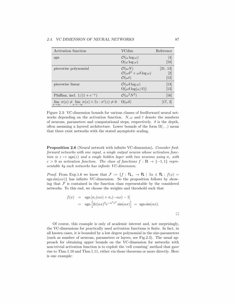
2.4. VC DIMENSION OF NEURAL NETWORKS 87
Activation function VCdim Reference
sgn O(ω logω) [4]Ω(ω logω) [18]
piecewise polynomial O(ωN) [21, 13]O(ωδ2 + ωδ logω) [2]O(ωt) [12]
piecewise linear O(ωδ logω) [13]Ω(ωδ log(ω/δ)
)[13]
Pfaffian, incl. 1/(1 + e−x) O(ω2N2) [16]
limx→∞
σ(x) 6= limx→−∞
σ(x) ∧ ∃z : σ′(z) 6= 0 Ω(ωδ) [17, 2]
Figure 2.3: VC-dimension bounds for various classes of feedforward neural net-works depending on the activation function. N,ω and t denote the numbersof neurons, parameters and computational steps, respectively. δ is the depth,often assuming a layered architecture. Lower bounds of the form Ω(. . .) meanthat there exist networks with the stated asymptotic scaling.
Proposition 2.6 (Neural network with infinite VC-dimension). Consider feed-forward networks with one input, a single output neuron whose activation func-tion is z 7→ sgn(z) and a single hidden layer with two neurons using σc withc > 0 as activation function. The class of functions f : R → −1, 1 repre-sentable by such networks has infinite VC-dimension.
Proof. From Exp.1.6 we know that F := f : R+ → R | ∃α ∈ R : f(x) =sgn sin(αx) has infinite VC-dimension. So the proposition follows by show-ing that F is contained in the function class representable by the considerednetworks. To this end, we choose the weights and threshold such that
f(x) = sgn [σc(αx) + σc(−αx)− 1]
= sgn[2c(αx)3e−α
2x2
sin(αx)]
= sgn sin(αx).
Of course, this example is only of academic interest and, not surprisingly,the VC-dimensions for practically used activation functions is finite. In fact, inall known cases, it is bounded by a low degree polynomial in the size-parameters(such as number of neurons, parameters or layers, see Fig.2.3). The usual ap-proach for obtaining upper bounds on the VC-dimension for networks withnon-trivial activation function is to exploit the ‘cell counting’ method that gaverise to Thm.1.10 and Thm.1.11, either via those theorems or more directly. Hereis one example:
88 CHAPTER 2. NEURAL NETWORKS
Theorem 2.9: VC-dimension—piecewise polynomial units
Consider an arbitrary architecture of a feedforward neural network withN neurons, m inputs, a single output and ω real parameters (i.e., weightsand threshold values). Let F be the set of functions from Rm to 0, 1that is representable within this architecture when every hidden neuronuses a piecewise polynomial activation function of degree at most d andwith at most p pieces and the output neuron uses σ(z) = 1z≥0. Then
V Cdim(F) ≤ 2ω[N log2 p+ log2
(8emax
δ + 1, 2dδ
)], (2.16)
where δ ∈ 0, . . . , N − 1 denotes the depth of the network.
Remark: Here, depth means the largest number of hidden neurons along anypath through the network. Hence, in a layered network δ is the number ofhidden layers. The number ω only counts distinct parameters, i.e., if weightsharing is used each weight is only counted once.
Proof. Considering the ω parameters as additional variables, the network can beregarded as a function Ψ : Rm×Rω → 0, 1. We interpret Ψ as a predicate andaim at expressing it as a Boolean combination of polynomial (in-)equalities, sothat Thm.1.10 applies. To this end, we have to bound the number of polynomialpredicates and their degree.
We use i ∈ 1, . . . , N to label the neurons, ordered so that the networkgraph contains no path from i to j < i. Denote by δ(i) ∈ 0, . . . , δ the maximaldepth of the i’th neuron in the network graph and by ai ∈ R the value of thei’th neuron’s output before applying the activation function.
Define I : R → 1, . . . , p so that I−1(j) is the interval corresponding tothe j’th piece in the domain of the piecewise polynomial activation function.Clearly, I(a) can be obtained from the truth values of p − 1 inequalities thatare linear in a. Since a1 is a quadratic function on Rm ×Rω the value of I(a1)can be obtained from p − 1 polynomial predicates over Rm × Rω of degree 2.Now consider I(ai). Conditioned on I(a1), . . . , I(ai−1), ai is a polynomial of
degree at most dδ(i) +∑δ(i)j=0 d
j =: deg(i) over Rm × Rω. Consequently, I(ai)can be determined from the truth values of p − 1 polynomial predicates overRm × Rω of degree deg(i). However, there are pi−1 different possibilities forI(a1), . . . , I(ai−1) leading to up to pi−1(p − 1) different polynomial predicatesthat, together with all previously obtained ones, determine I(ai).
So for determining I(aN−1) we need at most∑N−1j=1 pj−1(p− 1) = pN−1 − 1
polynomial predicates of degree at most deg(N−1). Finally, determining 1aN≥0
requires, for each value of I(a1), . . . , I(aN−1), one predicate that is linear in aNand thus polynomial of degree deg(N − 1) ≤ maxδ + 1, 2dδ. This is also themaximal degree of all the, in total less than pN , polynomial predicates. Withthese numbers, we can now enter Thm.1.10, which completes the proof.
2.5. RADEMACHER COMPLEXITY OF NEURAL NETWORKS 89
To summarize, if d and p are fixed, then
V Cdim(F) = O(ωN).
The proof technique is quite flexible in some directions: weight sharing or maxpooling as used in convolutional neural networks, as well as product units orsmall variations of the architecture are easily incorporated without changingthe picture. Under additional assumptions, such as a layered architecture orpiecewise linear activation functions, the above bound can even be improvedfurther, in the latter case down to O(ωδ logω). However, if the basic unitsare not piecewise algebraic, then ‘cell counting’ can become considerably moredifficult. For the logistic sigmoid σ(x) = (1 + e−x)−1 this can, however, still bedone leading to a bound based on Eq.(1.38). Fig.2.3 summarizes some of theknown results and points to the corresponding references.
2.5 Rademacher complexity of neural networks
Rademacher complexities of feedforward neural networks are most easily esti-mated, if the network obeys a layered structure. Then, with the help of theproperties of the (empirical) Rademacher complexities, which were summarizedin Thm.1.14, we can express the Rademacher complexities at the outputs of onelayer in terms of the ones corresponding to the foregoing layer:
Theorem 2.10: Rademacher complexity progression
Let a, b ∈ R, σ : R → R l-Lipschitz and assume F0 ⊆ RX is a setof functions that includes the zero function. The empirical Rademachercomplexity of F :=
x 7→ σ
(v +
∑mj=1 wjfj(x)
)∣∣ |v| ≤ a, ||w||1 ≤ b, fj ∈F0
)⊆ RX w.r.t. any point x ∈ Xn can be bounded in terms of the one
of F0 (w.r.t. the same point) by
R(F) ≤ l(
a√n
+ 2b R(F0)
). (2.17)
The factor 2 can be dropped if F0 = −F0.
Note: the number m of neurons in the layer enters the bound only indirectlyvia the || · ||1-constraint on the weights.
Proof. First, we exploit the Lipschitz-property of σ together with the corre-sponding property of the Rademacher complexity (point 5. in Thm.1.14) andobtain
R(F) ≤ l
nEσ
supv,w,fj
n∑
i=1
σi
v +
m∑
j=1
wjfj(xi)
. (2.18)
90 CHAPTER 2. NEURAL NETWORKS
Next, note that∑j wjfj ∈ b convF0−F0 =: G1. With G2 := x 7→ v | |v| ≤ a
we can regard the function class that appears in Eq.(2.18) as a sum of functionclasses so that (following property 3. in Thm.1.14) we can write
R(F) ≤ l(R(G1 + G2)
)= l
(R(G1) + R(G2)
)
≤ l
(a√n
+ 2b R(F0)
). (2.19)
In the second line, we used separate bounds for the two appearing empiricalRademacher complexities. On the hand, we used that (again by Thm.1.14)
R(G1) = bR(convF0−F0) = bR(F0−F0) = b(R(F0)+R(−F0)
)= 2bR(F0),
where the factor 2 is unnecessary if F0 = −F0. On the other hand, we usedthat R(G2) ≤ aE(|Z|)/n with Z :=
∑ni=1 σi, which in turn can be bounded via
Jensen’s inequality leading to
E[|Z|] ≤ E[Z2]1/2 =√n,
when exploiting the independence of the Rademacher variables.
In order to arrive at an upper bound for the empirical Rademacher complex-ity of en entire network, we can now apply the previous theorem recursively.Only the first layer requires a different treatment. One possibility is to use thefollowing ingredient:
Lemma 2.7. For b, c > 0, consider X := x ∈ Rd| ||x||∞ ≤ c and G := X 3x 7→ 〈x,w〉| ||w||1 ≤ b. The empirical Rademacher complexity of G w.r.t. anyz ∈ Xn can be bounded by
R(G) ≤ bc√n
√2 ln(2d). (2.20)
Proof. The proof is an application of Holder’s and Massart’s inequality:
nR(G) = Eσ
sup
w
d∑
j=1
n∑
i=1
σiwjzi,j
≤ b Eσ
[maxj
∣∣∣∣∣n∑
i=1
σizi,j
∣∣∣∣∣
]
= b Eσ
[maxa∈A
n∑
i=1
σiai
]
≤ bc√
2n ln(2d),
where we used Holder’s inequality in the first line, we set A := ±x1, . . . ,±xd ⊆Rn with (xj)i := zi,j in the second line and we exploited Massart’s inequalityfrom Eq.(1.54) with |A| ≤ 2d and ||xj ||2 ≤
√n||xj ||∞ ≤
√nc in the last line.
Combining Lemma 2.7 and Thm.2.10 then leads to the following:
2.6. TRAINING NEURAL NETWORKS 91
Corollary 2.8 (Rademacher complexity of layered network). Let a, b > 0 andX := x ∈ Rd| ||x||∞ ≤ 1. Fix a neural network architecture with δ hiddenlayers that implements F ⊆ RX s.t.
1. the activation function σ : R→ R is 1−Lipschitz and anti-symmetric, i.e.σ(−x) = −σ(x),
2. within every layer the vector w of weights satisfies ||w||1 ≤ b,
3. the moduli of the threshold values are bounded by a.
Then the empirical Rademacher complexity of F w.r.t. any z ∈ Xn then satisfies
R(F) ≤ 1√n
(bδ√
2 ln(2d) + a
δ−1∑
i=0
bi
). (2.21)
Note: σ = tanh for instance satisfies the requirements.
Proof. The result follows by replacing the function class G1 in the proof ofThm.2.10 with the class G of Lemma 2.7. Moreover, we use l = 1 as well asF0 = −F0 for every single layer.
The appearance of bδ, which bounds the product∏δi=1 ||wi||1 of norms of
the weight vectors of all layers, motivates the use of expressions of this type forregularization (as opposed to
∑δi=1 ||wi||22 in Tikhonov regularization).
2.6 Training neural networks
In this section, we will sketch the framework for training a neural network.Particular aspects and issues will then be discussed in greater detail in thefollowing sections. Training means to optimize the parameters of the model sothat that the model describes the training data well. Hence, we will have tochoose a loss function and an optimization algorithm. The architecture of thenetwork is supposed to be fixed.
Loss function. In case of regression, the most common choices for the lossfunction are the quadratic loss and the l1-distance. The latter is less sensitiveto ‘outliers’ than the former.
In case of classification, a common practice is the following: If Y is the set ofpossible classes, then instead of choosing one output node with values rangingin Y, one uses |Y| output nodes with real values, say z ∈ RY . To those theso-called softmax activation
σmax(z)y :=eβzy∑y∈Y e
βzy, β ∈ [0,∞) (2.22)
92 CHAPTER 2. NEURAL NETWORKS
is applied. Note that the softmax function is, in contrast to other activationfunctions, not a scalar function that can be applied to each coordinate sepa-rately, but maps RY into (0,∞)Y . More precisely, it turns a vector with realentries into a probability distribution that indicates the maximum entry in thelimit β →∞ and is a ‘soft’ version thereof otherwise. Usually, β = 1 is chosen.
Using such an output layer, the network maps every input x ∈ X to a prob-ability distribution, which can be interpreted as a quantification of the levelsof confidence. Let us denote the components of the distribution by p(y|x,w),where w is the collection of parameters the network depends on. The trainingdata set
((x1, y1), . . . , (xn, yn)
), on the other hand, defines an empirical distri-
bution p(y|xi) := δy,yi . For every data point xi the deviation between the twodistributions can be quantified using the Kullback-Leibler divergence
DKL
(p(xi)||p(xi, w)
):=
∑
y∈Yp(y|xi) log
p(y|xi)p(y|xi, w)
= − log p(yi|xi, w). (2.23)
To cast this into a loss function of the form defined in Sec.1.1 we can use themodified space of labels Y := RY with yi := (δy,yi)y∈Y . The loss function
L : Y × Y → [0,∞] giving rise to Eq.(2.23) then takes on the form
L(y, h(x)
)= −〈y, log h(x)〉,
which is sometimes simply called the log-loss. It is also known as cross entropy(when viewed as arising from the Kullback-Leibler divergence) or the negativelog-likelihood (when w 7→ p(y|x,w) is viewed as likelihood function for the pa-rameters w). Irrespective of these motivations the main reason for choosingthis type of loss-function is, however, that it appears to work well, on heuristicgrounds.
Algorithm The risk-function that has to be optimized as a function of theparameters, which we denote by w ∈ RN , is always an average of the loss-function over the n training data points. That is, formally we have to minimizea function of the form
f(w) =1
n
n∑
i=1
fi(w).
Gradient descent is a greedy (and probably the conceptually simplest) algorithmfor dealing with such an optimization problem: choose an initial point w0 ∈ RNand a (possibly time-dependent) step size α > 0 and then move along thesequence given by
wt+1 := wt − α∇f(wt),
where ∇f(wt) denotes the gradient of f at wt. In other words, follow thenegative gradient. Leaving aside issues of convergence, non-global minima andsaddle-points for the moment, there are (at least) two obstacles to overcome ifboth n and N are very large. Consider a naive numerical way of computing
2.7. BACKPROPAGATION 93
the gradient: due to linearity, the gradient is the sum of n gradients ∇fi(wt)each of which requires of the order of N function evaluations to be estimatednumerically sinceN is the dimension of the underlying space. Hence, before evena single step can be made downhill, n ·N function evaluations are required. Inour case, this means n · N evaluations (a.k.a. ‘forward passes’) of the neuralnetwork, which can easily be around 1014 — not very encouraging.
Two crucial ingredients reduce these nN evaluations, loosely speaking, to 2:
1. Backpropagation: For each fi the gradient can be computed analytically.Using the chain rule combined with some bookkeeping this requires onlyone forward and one ‘backward’ pass (and in this sense 2 evaluations).This routine is called ‘backpropagation’.
2. Stochastic gradient descent: Instead of computing the gradient of f ex-actly, one uses the gradients of the fi’s as stochastic approximation. Afterall, on average the gradients of the latter are equal to the gradient of theformer.
With these two ingredients, which will be discussed in detail in Sec. 2.7 and Sec.2.8, one possible way of proceeding is then as follows: start at a random initialpoint w0, choose a data point (xi, yi) at random (in practice, usually withoutreplacement), compute the gradient of the corresponding fi using backpropa-gation, update w by moving opposite to that gradient, and then iterate thisprocedure.
One complete run over the set of n training data points is called an epoch.Instead of making n steps in parameter space during an epoch, it is often ad-vantageous to form disjoint groups, so-called mini-batches, of k data points eachand to average the corresponding k gradients before making one step. In thisway, the stochastic gradient becomes less ‘noisy’, the step size can be increasedand, since the gradients within one mini-batch are computed using the sameparameters but different data points, it opens a door for parallelization.
2.7 Backpropagation
... exact computation of the gradient...... to be completed ...Consider a layered feedforward neural network whose layers will be labeled by
an upper or lower index l ∈ 0, . . . ,m. Here, the 0’th layer corresponds to theinput and the m’th to the output. Nl will be the number of neurons in the l’thlayer. By wljk we will denote the weight that corresponds to the connection from
the k’th neuron in layer l−1 to the j’th neuron in layer l. Similarly, blj will be the
threshold value of the j’th neuron in layer l. The vector xl, whose componentsxlj are the outputs of the neurons of the l’th layer, can then be expressed in
matrix/vector notation as xl = σ(wlxl−1 + bl), where the activation function σis applied component-wise. We introduce a separate variable zl := wlxl−1 + bl
to denote the output before application of the activation function.
94 CHAPTER 2. NEURAL NETWORKS
Consider a function f : RNm → R that maps the output xm to a realnumber—such as the loss function, which acts as L(y, xm) =: f(xm) for a fixedpair (x0, y) of the training data. By expanding xm in terms of previous layersand the corresponding weights and threshold values, we may interpret f asa function of different kinds of variables. In particular, we will consider themappings (w, b) 7→ f(xm), xl 7→ f(xm) and zm 7→ f(xm). Abusing notation allthese mappings will be denoted by f .
Our aim is to compute the partial derivatives of f w.r.t. all weights andthreshold values. To this end, we introduce intermediate quantities δlj := ∂f
∂zljin
terms of which all the sought derivatives will be expressed by use of the chainrule. The latter is also central in computing the δlj ’s themselves. Beginningwith the output layer, we obtain
δmj =∑
k
∂f
∂xmk
∂xmk∂zmj
= σ′(zmj )∂f
∂xmj, (2.24)
where the summation runs over all neurons in the considered layer. Next, weshow that δl can be expressed in terms of δl+1, so that all δ’s can be computedby going layerwise backwards from the output layer:
δlj =∂f
∂zlj=
∑
k
∂f
∂zl+1k
∂zl+1k
∂zlj
=∑
k
δl+1k wl+1
kj σ′(zlj). (2.25)
Finally, we can express the sought derivatives in terms of the δ’s:
∂f
∂blj=
∑
k
∂f
∂zlk
∂zlk∂blj
= δlj , (2.26)
∂f
∂wljk=
∑
i
∂f
∂zli
∂zli∂wljk
= δlj xl−1k . (2.27)
As a result we obtain that in order to compute the partial derivatives of f w.r.t.all weights and threshold values it suffices to run the network once forward (toobtain all x’s and z’s) and once ’backwards’ (to obtain the δ’s). This has to becontrasted with the naive approach, where for every individual partial derivativethe network had to be evaluated twice already.
... add: approach via Lagrange duality ...
2.8 Gradient descent and descendants
This section is a first excursion into optimization theory. Motivated by but notrestricted to the training of neural networks, we will have a look at iterativeoptimization methods that can be regarded as descendants of the gradient de-scent method. The common strategy of these methods for minimization of a
2.8. GRADIENT DESCENT AND DESCENDANTS 95
function f : Rd → R is as follows. Start at a randomly/cleverly chosen pointx0 ∈ Rd and then step-by-step move along a path given by xt+1 = xt + ∆t
that is iteratively constructed and ideally ‘descending’ regarding the value ofthe function. Here, the increment ∆t depends on (stochastic approximationsof) local properties of the function at xt and, in some cases, on the history ofthe path up to that point. The central ‘local property’ is the gradient of thefunction at xt. Using higher order derivatives is in principle beneficial, but thecomputational costs per step often exceed the feasibility limit if the problem athand is very high-dimensional (especially, if d 105)4.
Gradient descent and its descendants are ideally suited for the realm of highdimensions. The main reason for this is that its oracle complexity is essentiallydimension-free. That is, the number of times the gradient (or function value)has to be computed before convergence is achieved up to some accuracy ε, isessentially independent of the dimension. In fact, all bounds that are derivedin this section are independent of d. They do involve constants characterizingcontinuity or convexity properties of the function and, of course, those mayimplicitly depend on the dimension. Also the cost of each evaluation of thefunction or of its gradient depends on d. In contrast to other methods (suchas interior point or ellipsoid methods, which when applicable would have muchfaster convergence) gradient descent techniques, however, do not add additionaldimension factors.
Steepest descent Before going into details, let us consider different choicesfor the increment ∆t from a more distant perspective. Assuming differentia-bility, we can approximate the function in a neighborhood around a point xas
f(x−∆) ' f(x) + 〈∆,∇f(x)〉.
Aiming at a descending path, a reasonable choice for the increment ∆ is thusone that minimizes the inner product with the gradient. This will determine thedirection of steepest descent. Bounding the step size by α > 0, which is ideallychosen so that the linear approximation is still reasonably good, this means
∆ = argmin〈∆,∇f(x)〉
∣∣ ||∆|| ≤ α. (2.28)
At this point, we have to choose the norm (or even a more general normalizingfunctional) that constrains ∆. Suppose we choose ||x|| := 〈x, Px〉1/2 for somepositive definite matrix P . Then
∆ = − αP−1∇f(x)
||P−1∇f(x)||(2.29)
solves the minimization problem. If P = 1, which means that || · || = || · ||2 is theEuclidean norm, then ∆ equals the step size times the negative gradient. Thisis the choice made in the gradient descent method. However, the Euclideannorm may not be the most natural or most relevant choice. For instance, if
4Neural networks are trained with currently up to d ∼ 1011 parameters.
96 CHAPTER 2. NEURAL NETWORKS
we regard the constraint due to α as a guarantee for the quality of the linearapproximation, then the norm where P equals the Hessian of f at x seemsto be more appropriate. In fact, this is the choice made in Newton’s method.Other choices can be well-motivated, as well. Having in mind generalization,regularization or sparsity, one may for instance want to have preferred directions,which are then reflected in the chosen normalizing functional. We will, however,now close this door again and have a closer look at the relatives of gradientdescent, where the Euclidean norm lies beneath the update rule xt+1 = xt −α∇f(xt).
Gradient descent For gradient descent to become a meaningful algorithm,the gradient should not be too wild. One way to formalize this is to demandthe gradient to be Lipschitz continuous. The following Lemma summarizes twocentral implications of this assumption.
Lemma 2.9. Let x, y ∈ Rd and f ∈ C1(Rd) be such that ∇f is L-Lipschitz.Then the following holds with the norm induced by the inner product:
1.∣∣f(x)− f(y)− 〈∇f(x), x− y〉
∣∣ ≤ L2 ||x− y||
2.
2. If f is convex: f(x)− f(y)− 〈∇f(x), x− y〉 ≤ − 12L ||∇f(y)−∇f(x)||2.
Note: The first inequality shows how the function can be bounded by aquadratic function. The second inequality can be regarded as a strengtheningof the convexity condition. In fact, if we set the r.h.s. of the second inequalityto zero (L = ∞), then validity of the inequality for all x, y is equivalent toconvexity of f . Geometrically, this is the tangent plane lying below the graph.
Proof. 1. By the fundamental theorem of calculus, we can write f(x)− f(y) =∫ 1
0〈∇f
(y + t(x − y)
), x − y〉dt. With the help of Cauchy-Schwarz and the
Lipschitz-property of the gradient, this leads to
∣∣f(x)− f(y)− 〈∇f(x), x− y〉∣∣ ≤
∫ 1
0
∣∣∣〈∇f(y + t(x− y)
)−∇f(x), x− y〉
∣∣∣dt
≤∫ 1
0
‖∇f(y + t(x− y)
)−∇f(x)‖ ‖x− y‖dt
≤∫ 1
0
tL‖x− y‖2dt =L
2‖x− y‖2.
2. To prove the second inequality, we introduce the auxiliary variable z :=y + (∇f(x)−∇f(y))/L. Then
f(x)− f(y) = f(x)− f(z) + f(z)− f(y)
≤ 〈∇f(x), x− z〉+ 〈∇f(y), z − y〉+L
2||z − y||2
= 〈∇f(x), x− y〉 − 1
2L||∇f(x)−∇f(y)||2, (2.30)
2.8. GRADIENT DESCENT AND DESCENDANTS 97
where the step to the second line used convexity of f for the first two terms andexploited the just proven inequality 1. to bound f(z)− f(y).
If we insert x = xt and y = xt+1 = xt−α∇f(xt) into inequality 1. of Lemma2.9, we obtain, after collecting terms
f(xt)− f(xt+1) ≥ α(
1− αL
2
)||∇f(xt)||2. (2.31)
Assuming that the gradient is not vanishing, the r.h.s. of Eq.(2.31) is posi-tive, which means that gradient descent is indeed descending, if α ∈ (0, 2/L).Furthermore, it is maximal when α = 1/L. If the update rule would bext+1 = xt − P∇f(xt) for some positive matrix P , then the operator norm||P ||∞ would play the role of α and ||P ||∞ ∈ (0, 2/L) would imply monotonic-ity. We will, however, not pursue this direction further and stick to the standardupdate. The following theorem collects the implications of Eq.(2.31). It shows,in particular, that under reasonable assumptions gradient descent converges toa stationary point.
Theorem 2.11: Gradient descent - convergence to stationarity
Let f ∈ C1(Rd) have L-Lipschitz gradient and consider the sequencext+1 = xt − α∇f(xt) for some α ∈ (0, 2/L) and x0 ∈ Rd. Then
1. f(xt+1) < f(xt) unless ∇f(xt) = 0.
2. If f is bounded from below, then ∇f(xt)→ 0 for t→∞.
3. If f attains a minimum at x∗ and we choose α = 1/L, then for allT ∈ N:
mint<T||∇f(xt)||2 ≤
2L(f(x0)− f(x∗)
)
T. (2.32)
Proof. 1. follows immediately from Eq.(2.31). In order to arrive at 2. and 3.
we take the sum∑T−1t=0 over Eq.(2.31). Then
f(x0)− f(xT ) ≥ α
(1− αL
2
) T−1∑
t=0
||∇f(xt)||2
≥ α
(1− αL
2
)T mint<T||∇f(xt)||2.
By assumption, the l.h.s. in the first line is uniformly bounded for all T . So wecan take the limit T →∞ and observe that the r.h.s. can only remain boundedif ∇f(xt)→ 0. 3. follows from f(xT ) ≥ f(x∗) when inserting α = 1/L.
In order to obtain results that are stronger than mere (and rather slow) con-vergence towards a stationary point, we need stronger assumptions. An often
98 CHAPTER 2. NEURAL NETWORKS
made assumption is strong convexity (see Def.1.27). An alternative and slightlymore general condition is the Polyak- Lojasiewicz inequality for some µ > 0:
∀x ∈ Rd :1
2||∇f(x)||2 ≥ µ
(f(x)− f(x∗)
), (2.33)
where f : Rd → R is supposed to attain a global minimum at x∗. Note thatthe validity of this inequality for µ > 0 implies that every stationary point is aglobal minimum. The condition is independent of convexity5, but it is impliedby µ-strong convexity:
Lemma 2.10 (Polyak- Lojasiewicz from strong convexity). If there is a µ > 0for which f : Rd → R is µ−strongly convex, then Eq.(2.33) holds for everysubgradient.
Note: recall that v ∈ Rd is a subgradient of f at x iff
∀y ∈ Rd : f(y) ≥ f(x) + 〈v, y − x〉. (2.34)
If f is convex and continuous, then at every point x the set of subgradients isnon-empty. If it is in addition differentiable at x, then the subgradient at x isunique and given by the gradient ∇f(x). Where convenient, we will use thenotation ∇f(x) also for subgradients in the non-differentiable case.
Proof. By definition f is µ-strongly convex iff the map x 7→ f(x)− µ||x2||/2 isconvex. Applied to this map, Eq.(2.34) reads
f(y) ≥ f(x) +µ
2||x− y||2 + 〈∇f(x), y − x〉. (2.35)
Minimizing both sides w.r.t. y then gives f(x∗) ≥ f(x)−||∇f(x)||2/(2µ), whichis the Polyak- Lojasiewicz inequality.
Theorem 2.12: Gradient descent - exponential convergence
Let f ∈ C1(Rd) satisfy the Polyak- Lojasiewicz inequality in Eq.(2.33) forsome µ > 0, have L−Lipschitz gradient and a global minimum attainedat x∗. For α ∈ [0, 2/L] and x0 ∈ Rd the sequence xt+1 := xt − α∇f(xt)satisfies for all T ∈ N:
f(xT )− f(x∗) ≤(
1 + αµ(αL− 2))T (
f(x0)− f(x∗))
(2.36)
=(
1− µ
L
)T (f(x0)− f(x∗)
), for α = 1/L.
Note: Depending on the community this type of convergence is called linear,exponential or geometric convergence.
5For instance, x 7→ x2 + 3(sinx)2 is not convex but satisfies Eq.(2.33) with µ = 1/32 and,on the other side, x 7→ |x| is convex but does not satisfy Eq.(2.33) for any µ > 0.
2.8. GRADIENT DESCENT AND DESCENDANTS 99
Proof. We begin with applying inequality 1. from Lemma 2.9 and inserting theupdate rule. Then
f(xt+1) ≤ f(xt) + 〈∇f(xt), xt+1 − xt〉+L
2||xt+1 − xt||2
= f(xt)− α(1− αL/2) ||∇f(xt)||2
≤ f(xt) + αµ(αL− 2)(f(xt)− f(x∗)
), (2.37)
where the last step used the Polyak- Lojasiewicz condition. Subtracting f(x∗)from both sides of the inequality and applying it recursively then leads to theclaimed result.
Note that the speed of convergence in this bound is governed by L/µ. Iff ∈ C2, then locally L/µ corresponds to the condition number of the Hes-sian. So, loosely speaking, the better the Hessian is conditioned, the faster theconvergence. Note that also Newtons methods appears well-motivated in thislight, since it aims at minimizing the condition number of the Hessian by locallytransforming it to the identity matrix. In fact, in this way, Newton’s methodachieves super-exponential convergence.
Stochastic gradient descent We will now consider variants of the stochasticgradient descent method, where the gradient is replaced by a stochastic approx-imation. This is no longer a strict ‘descent’, since the direction of the incrementnow becomes a random variable, which is only proportional to the gradient onaverage.
Theorem 2.13: Stochastic gradient descent - fixed step size
Let f ∈ C1(Rd) satisfy the Polyak- Lojasiewicz inequality in Eq.(2.33) forsome µ > 0, have L−Lipschitz gradient and a global minimum attained atx∗. For any T ∈ N, x ∈ Rd let g1(x), . . . , gT (x) be i.i.d. random variableswith values in Rd such that E[gt(x)] = ∇f(x). With x0 ∈ Rd considerthe sequence xt+1 := xt − αgt(xt).
1. If ∀x, t : E[||gt(x)||2
]≤ γ2 and α ∈ [0, 1/(2µ)], then
E[f(xT )
]− f(x∗) ≤ (1− 2µα)T
(f(x0)− f(x∗)
)+Lαγ2
4µ. (2.38)
2. If ∀x, t : E[||gt(x)||2
]≤ β2||∇f(x)||2 and α = 1/(Lβ2), then
E[f(xT )
]− f(x∗) ≤
(1− µ
Lβ2
)T (f(x0)− f(x∗)
). (2.39)
Proof. We begin as in the proof of Thm.2.12 and insert the update rule intoinequality 1. from Lemma 2.9. In this way, we obtain
f(xt+1) ≤ f(xt)− α〈∇f(xt), gt(xt)〉+ α2L||gt(xt)||2/2.
100 CHAPTER 2. NEURAL NETWORKS
Next, we take the expectation value w.r.t. gt conditioned on fixed g1, . . . , gt−1:
Egt
[f(xt+1)
]≤ f(xt)− α||∇f(xt)||2 + α2LEgt
[||gt(xt)||2
]/2. (2.40)
In order to prove Eq.(2.38) we proceed with bounding the last term in Eq.(2.40)in terms of γ2 and the second term using the Polyak- Lojasiewicz inequality.Subtracting f(x∗) from both sides of the inequality and taking the expectationvalue also w.r.t. g1, . . . , gt−1 then leads to
E[f(xt+1)− f(x∗)
]≤ E
[f(xt)− f(x∗)
](1− 2µα) + α2Lγ2/2.
Now we can apply the resulting inequality recursively, so that with T = t+ 1:
E[f(xT )− f(x∗)
]≤(f(x0)− f(x∗)
)(1− 2µα)T +
α2Lγ2
2
T−1∑
k=0
(1− 2µ)k,
which, after upper bounding the sum by the geometric series, becomes Eq.(2.38).To obtain Eq.(2.39) we proceed similarly from Eq.(2.40), but now bound
the last term in terms of β2||∇f(xt)||2 and then apply the Polyak- Lojasiewiczinequality. Again, we subtract f(x∗) from both sides of the resulting inequalityand take the expectation value w.r.t. the remaining random variables. Thisleads to
E[f(xt+1)− f(x∗)
]≤ E
[f(xt)− f(x∗)
](1− µα(2− Lαβ2)
),
which can be iterated and then leads to Eq.(2.39) after inserting α = 1/(Lβ2).
Eq.(2.38) exhibits a central aspect of stochastic gradient descent: a fragilerelation between the speed of convergence on large scales and the preventionof convergence by stochastic noise. One the one hand, the first term on ther.h.s. in Eq.(2.38) motivates a large steps size that guarantees fast conver-gence. The second term, on the other hand, shows that beyond a certain value,which grows with the step size, there is no convergence anymore. This is wherestochastic noise dominates (cf. Fig.2.4). In the second statement of the theo-rem, Eq.(2.39), by assumption, the stochastic noise gets suppressed more andmore when coming closer to the minimum. This implies that all stochastic gra-dients have to vanish simultaneously at the minimum. As this is an extremelystrong (and typically unjustified) assumption, we will not pursue it further afterhaving mentioning that the two cases can easily be combined into one assumingthat ∀x, t : E
[||gt(x)||2
]≤ β2||∇f(x)||2 + γ2.
Eq.(2.38) is consistent with a heuristic strategy that is often used in practice:use constant step size for a long time (until stochastic noise prevents progress),then halve the step size and iterate this procedure.
The next theorem shows that appropriately decreasing the step size canindeed guarantee convergence when the function is convex. For this, neitherdifferentiability nor the Polyak- Lojasiewicz condition are necessary. The state-ment is proven under the additional constraint, that the path remains inside agiven compact convex set.
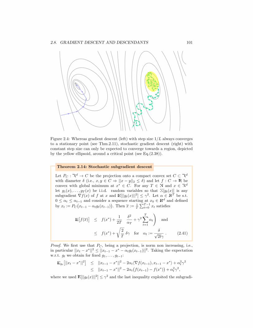
2.8. GRADIENT DESCENT AND DESCENDANTS 101
Figure 2.4: Whereas gradient descent (left) with step size 1/L always convergesto a stationary point (see Thm.2.11), stochastic gradient descent (right) withconstant step size can only be expected to converge towards a region, depictedby the yellow ellipsoid, around a critical point (see Eq.(2.38)).
Theorem 2.14: Stochastic subgradient descent
Let PC : Rd → C be the projection onto a compact convex set C ⊂ Rdwith diameter δ (i.e., x, y ∈ C ⇒ ||x − y||2 ≤ δ) and let f : C → R beconvex with global minimum at x∗ ∈ C. For any T ∈ N and x ∈ Rdlet g1(x), . . . , gT (x) be i.i.d. random variables so that E[gt(x)] is anysubgradient ∇f(x) of f at x and E[||gt(x)||2] ≤ γ2. Let α ∈ RT be s.t.0 ≤ αt ≤ αt−1 and consider a sequence starting at x0 ∈ Rd and defined
by xt := PC(xt−1 − αtgt(xt−1)
). Then x := 1
T
∑T−1t=0 xt satisfies
E[f(x)
]≤ f(x∗) +
1
2T
(δ2
αT+ γ2
T∑
t=1
αt
)and
≤ f(x∗) +
√2
Tδγ for αt :=
δ√2tγ
. (2.41)
Proof. We first use that PC , being a projection, is norm non increasing, i.e.,in particular ||xt − x∗||2 ≤ ||xt−1 − x∗ − αtgt(xt−1)||2. Taking the expectationw.r.t. gt we obtain for fixed g1, . . . , gt−1:
Egt
[||xt − x∗||2
]≤ ||xt−1 − x∗||2 − 2αt〈∇f(xt−1), xt−1 − x∗〉+ α2
tγ2
≤ ||xt−1 − x∗||2 − 2αt(f(xt−1)− f(x∗)
)+ α2
tγ2,
where we used E[||gt(x)||2] ≤ γ2 and the last inequality exploited the subgradi-
102 CHAPTER 2. NEURAL NETWORKS
ent inequality, Eq.(2.34). Taking the expectation also w.r.t. to g1, . . . , gt−1 wecan rewrite the resulting inequality as
E[f(xt−1)
]− f(x∗) ≤ γ2
2αt +
1
2αtE[||xt−1 − x∗||2 − ||xt − x∗||2
]. (2.42)
As an intermediate step, consider the sum
T∑
t=1
1
αt
(||xt−1 − x∗||2 − ||xt − x∗||2
)
=1
α1||x0 − x∗||2 −
1
αT||xT − x∗||2 +
T∑
t=2
(1
αt− 1
αt−1
)||xt−1 − x∗||2
≤ δ2
α1+ δ2
T∑
t=2
(1
αt− 1
αt−1
)=
δ2
αT, (2.43)
where the inequality uses that the αt’s are positive and non-increasing togetherwith the finite diameter of the set C that contains all considered points. Usingconvexity of f in combination with Eq.(2.42) and Eq.(2.43) we obtain
E[f(x)
]≤ 1
T
T∑
t=1
E[f(xt−1)]
≤ f(x∗) +1
2T
(δ2
αT+ γ2
T∑
t=1
αt
).
Finally, after inserting αt = δ/(√
2tγ), we can simplify the expression by using
that∑Tt=1 t
−1/2 ≤∫ T
0t−1/2dt = 2
√T , which then leads to Eq.(2.41).
2.9 (Un)reasonable effectiveness—optimization
We begin with two examples that show how hard problems can arise—even inthe absence of a complex architecture and without a large number of non-globalminima or saddle points.
NP-hardness of empirical risk minimization Consider an arbitrary graphG = (V,E) whose vertices are numbered so that V = 1, . . . , d. Assign a setSG ∈
0, 1|V | ×0, 1
nwith n := |V |+ |E|+ 1 to the graph in the following
way: denoting by ei ∈ 0, 1|V | the unit vector whose i’th component is equalto one, we set SG = (ei, 0), (ei + ej , 1), (0, 1)i∈V,(i,j)∈E .
Recall that G is called 3-colorable iff there exists a map χ : V → 1, 2, 3with the property that (i, j) ∈ E ⇒ χ(i) 6= χ(j). That is, there is an assignmentof ’colors’ to vertices such that no pair connected by an edge has the same color.
2.9. (UN)REASONABLE EFFECTIVENESS—OPTIMIZATION 103
Proposition 2.11. Consider feedforward neural networks with d inputs, a sin-gle hidden layer with three neurons and a single output neuron. Assume allactivation functions are σ(z) = 1z≥0 and that the output neuron has all weights
and the threshold fixed so that it acts as x 7→ σ(∑3i=1(xi−1)). Let Fd ⊆ 0, 1R
d
be the function class that can be represented by such networks. Then for anygraph G with d vertices there is an f ∈ Fd that correctly classifies SG iff G is3-colorable.
Proof. Note first that the output neuron is set up so that it ‘fires’ iff all threehidden neurons do so. Assume G is 3-colorable via χ : V → 1, 2, 3. Choosethe weight wl,i that connects the i’th input and the l’th hidden neuron so thatwl,i = −1 if χ(i) = l and wl,i = 1 otherwise. The threshold values of thethree hidden neurons are all set to 1/2, which leads to an f ∈ Fd that can becharacterized by
f(x) = 1 ⇔ ∀l ∈ 1, 2, 3 :∑
k
wl,kxk ≥ −1
2.
Now we have to verify that f correctly classifies SG. Clearly, f(0) = 1. It alsoholds that f(ei) = 0 since if χ(i) = l, then wl,i = −1 so that
∑k wl,k(ei)k =
wl,i 6≥ −1/2. In order to verify f(ei + ej) = 1 for all (i, j) ∈ E, note that forany l ∈ 1, 2, 3 we have χ(i) 6= l ∨ χ(j) 6= l since χ is a coloring. Therefore∑k wl,k(ei + ej)k = wl,i + wl,j is non-negative for all l.Let us now show the converse implication and assume that there is an f ∈ Fd
that correctly classifies SG. Associating a half space Hl to each of the hiddenPerceptrons we can express this assumption as f−1(1) = H1 ∩H2 ∩H3 =: Hwhere 0 ∈ H, ∀(i, j) ∈ E : ei + ej ∈ H and ∀i ∈ V : ei 6∈ H. We defineχ(i) := minl|ei 6∈ Hl and claim that this is a 3-coloring. First note that due toconvexity of H and the fact that H contains the origin, we have (ei+ej)/2 ∈ Hfor every edge (i, j) ∈ E. Suppose, aiming at a contradiction, that there wouldbe an edge for which χ(i) = χ(j) = l. Then since ei, ej 6∈ Hl this would, againby convexity, imply that (ei + ej)/2 6∈ Hl – a contradiction.
Via reduction from 3-SAT, the 3-coloring problem is known to be NP-complete. Hence, the above Proposition shows that (NP-)hard problems canalready be found in instances of empirical risk minimization for neural net-works with very simple architecture. However, admittedly, the example is ofcombinatorial nature and uses an activation function that has been practicallyabandoned—essentially for this reason. So let us consider a ‘smoother’ problem...
NP-hardness of classifying stationary points An instructive example forunderstanding, when and which problems can be hard, is given by homogeneousquartic polynomials. For a symmetric matrix Q ∈ Zd×d, define f : Rd → R as
f(x) :=
d∑
i,j=1
Qi,jx2ix
2j . (2.44)

104 CHAPTER 2. NEURAL NETWORKS
At x = 0 both the gradient and the Hessian of f are zero. Hence, x = 0 isa stationary point, but the Hessian does not provide any information aboutwhether it is a minimum, maximum or merely a saddle point. We do know,however, that there is a global minimum at x = 0 if there is a local minimum:suppose it not global, i.e., there is an x with f(x) < 0, then R 3 λ 7→ f(λx) =λ4f(x) shows that it cannot be a local minimum, either. Moreover, it showsthat f is unbounded from below iff 0 is not a local minimum. Consequently, thetwo following problems are equivalent:
P1 Does f have a saddle point at 0 that is not a local minimum?
P2 Is f unbounded from below?
A negative answer to both these questions is a property of the matrix Q thatis called copositivity. That is, Q is copositive by definition if 〈z,Qz〉 ≥ 0 for allentrywise non-negative z. By relating the problem to one (e.g. the subset-sumproblem) that is known to be NP complete, one can prove that showing thatQ is not copositive is NP complete, as well [?]. Hence, despite the apparentsimplicity of f , both P1 and P2 are NP-complete problems. Note that thehardness in this case does not come from a large number of non-global minimaor saddle points. It is simply the growing dimension that makes the problemhard.
Saddle points
Lemma 2.12 (Center-stable manifold theorem [?, ?]). Let g : Rd → Rd be alocal C1-diffeomorphism with fixed point z = g(z). Let the Jacobian Dg(z) havek eigenvalues (counting algebraic multiplicities) of modulus less than or equalto one. Then there is a k−dimensional manifold Wz ⊆ Rd and an open ball Bzaround z s.t. g(Wz) ∩ Bz ⊆ Wz and if gt(x) ∈ Bz holds for all t ∈ N0, thenx ∈Wz.
Wz is called center-stable manifold.
Lemma 2.13 (Gradient descent update is a diffeomorphism). Let f ∈ C2(Rd)be such that ∇f is L-Lipschitz w.r.t. the Euclidean norm. If α ∈ (0, 1/L), theng(x) := x− α∇f(x) defines a C1-diffeomorphism on Rd.
Proof. We first prove injectivity. Suppose g(x) = g(y), which is equivalent to(x− y)/α = ∇f(x)−∇f(y). Taking norms and using the Lipschitz property ofthe gradient, this implies ||x− y||/α ≤ L||x− y||. Since 1/α > L this can onlyhold if x = y. So g is injective.
It remains to show that g, which is C1 by construction, is a local C1-diffeomorphism. To this end, note first that ∇f being L-Lipschitz is equivalentto ∀x : ∇2f(x) ≤ L1, i.e., the eigenvalues of the Hessian being not larger than L.This implies that the Jacobian of g, which is Dg(x) = 1−α∇2f(x) is invertible.By the inverse function theorem, g is thus a local C1-diffeomorphism.
2.10. DEEP NEURAL NETS 105
Theorem 2.15: Almost no convergence to strict saddle points
Let f ∈ C2(Rd) be such that ∇f is L-Lipschitz w.r.t. the Euclidean normand define g(x) := x − α∇f(x) for some α ∈ (0, 1/L). Let S ⊆ Rd bethe set of stationary points of f for which the Hessian has at least onenegative eigenvalue. Then S∞ := x ∈ Rd|∃z ∈ S : limt→∞ gt(x) = zhas Lebesgue measure zero.
Proof. First note that if z ∈ S is such a stationary point, then the JacobianDg(z) has strictly less than d eigenvalues of modulus at most one. Consequently,the manifold Wz that corresponds to z in the center-stable manifold theorem(Lemma 2.12) has reduced dimension. Define B :=
⋃z∈S Bz with the balls from
Lemma 2.12. By the Lindelof covering theorem, there is a countable subcover.That is, there exist zi ∈ S so that S ⊆ B =
⋃i∈NBzi . If gt(x) converges to
z ∈ S, then z ∈ Bzi for some zi ∈ S and there is a τ ∈ N so that for allt ≥ τ we have that gt(x) ∈ Bzi . Therefore, by Lemma 2.12, gτ (x) ∈ Wzi ,which means that x ∈ g−τ (Wzi). Arguing like this for all x ∈ S∞ we obtainS∞ ⊆
⋃i∈N
⋃τ∈N g
−τ (Wzi). This is a countable union of sets of measure zero(as the differentiable map g−τ maps nullsets to nullsets), so it has measure zero,as well.
Non-global minima ... to be written ...
2.10 Deep neural nets
... to be completed. Missing: history, vanishing gradient problem, convolutionaland residual nets ...
Representation benefits of deep networks Define F(m, l) ⊆ RR as theset of functions that can be represented by a feedforward neural network withl layers, m neurons within every hidden layer, a single neuron at the outputand the rectified linear unit σR(z) := max0, z as activation function. Inorder to make an f ∈ F(m, l) into a classifier, define f(x) := 1f(x)≥1/2 and
let R(f) := 1|S|∑
(x,y)∈S 1f(x)6=y be the corresponding empirical risk w.r.t. a
training data set S.
Theorem 2.16: Exponential benefit of deep networks
Let k ∈ N, n = 2k and S :=((xi, yi)
)n−1
i=0with xi := i/n and yi := i mod 2.
1. There is an h ∈ F(2, 2k) for which R(h) = 0.
2. Ifm, l ∈ N andm ≤ 2k−2l −1, then R(f) ≥ 1
6 holds for all f ∈ F(m, l).
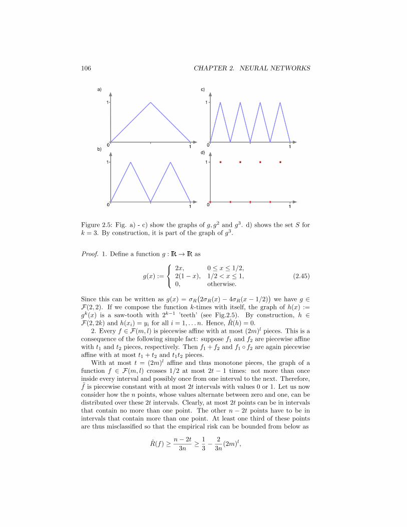
106 CHAPTER 2. NEURAL NETWORKS
Figure 2.5: Fig. a) - c) show the graphs of g, g2 and g3. d) shows the set S fork = 3. By construction, it is part of the graph of g3.
Proof. 1. Define a function g : R→ R as
g(x) :=
2x, 0 ≤ x ≤ 1/2,2(1− x), 1/2 < x ≤ 1,0, otherwise.
(2.45)
Since this can be written as g(x) = σR(2σR(x) − 4σR(x − 1/2)
)we have g ∈
F(2, 2). If we compose the function k-times with itself, the graph of h(x) :=gk(x) is a saw-tooth with 2k−1 ’teeth’ (see Fig.2.5). By construction, h ∈F(2, 2k) and h(xi) = yi for all i = 1, . . . n. Hence, R(h) = 0.
2. Every f ∈ F(m, l) is piecewise affine with at most (2m)l pieces. This is aconsequence of the following simple fact: suppose f1 and f2 are piecewise affinewith t1 and t2 pieces, respectively. Then f1 + f2 and f1 f2 are again piecewiseaffine with at most t1 + t2 and t1t2 pieces.
With at most t = (2m)l affine and thus monotone pieces, the graph of afunction f ∈ F(m, l) crosses 1/2 at most 2t − 1 times: not more than onceinside every interval and possibly once from one interval to the next. Therefore,f is piecewise constant with at most 2t intervals with values 0 or 1. Let us nowconsider how the n points, whose values alternate between zero and one, can bedistributed over these 2t intervals. Clearly, at most 2t points can be in intervalsthat contain no more than one point. The other n − 2t points have to be inintervals that contain more than one point. At least one third of these pointsare thus misclassified so that the empirical risk can be bounded from below as
R(f) ≥ n− 2t
3n≥ 1
3− 2
3n(2m)l,
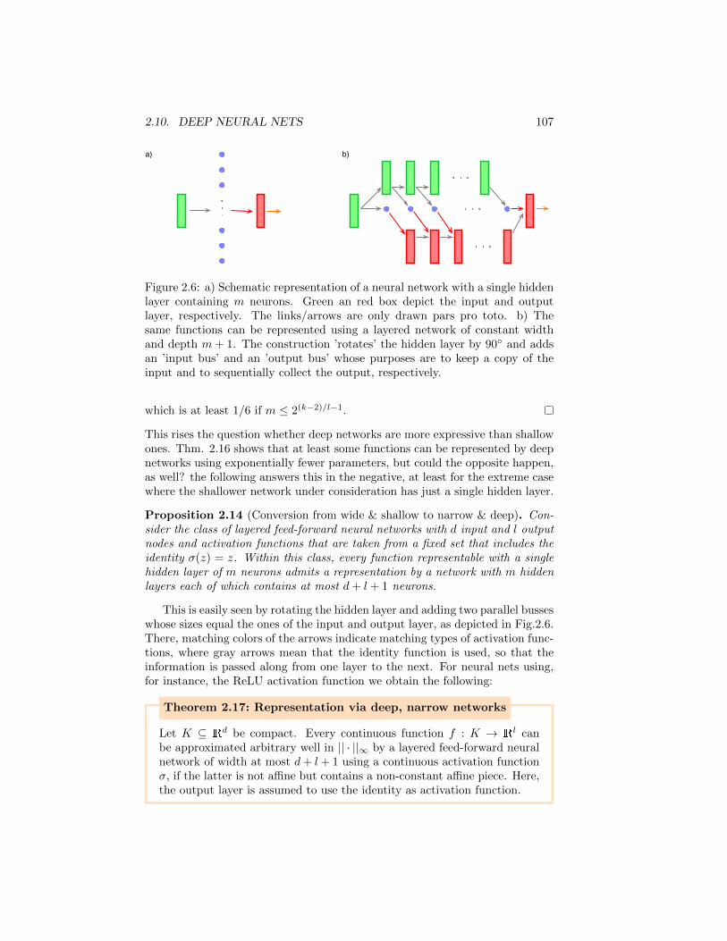
2.10. DEEP NEURAL NETS 107
a) b)
Figure 2.6: a) Schematic representation of a neural network with a single hiddenlayer containing m neurons. Green an red box depict the input and outputlayer, respectively. The links/arrows are only drawn pars pro toto. b) Thesame functions can be represented using a layered network of constant widthand depth m+ 1. The construction ’rotates’ the hidden layer by 90 and addsan ’input bus’ and an ’output bus’ whose purposes are to keep a copy of theinput and to sequentially collect the output, respectively.
which is at least 1/6 if m ≤ 2(k−2)/l−1.
This rises the question whether deep networks are more expressive than shallowones. Thm. 2.16 shows that at least some functions can be represented by deepnetworks using exponentially fewer parameters, but could the opposite happen,as well? the following answers this in the negative, at least for the extreme casewhere the shallower network under consideration has just a single hidden layer.
Proposition 2.14 (Conversion from wide & shallow to narrow & deep). Con-sider the class of layered feed-forward neural networks with d input and l outputnodes and activation functions that are taken from a fixed set that includes theidentity σ(z) = z. Within this class, every function representable with a singlehidden layer of m neurons admits a representation by a network with m hiddenlayers each of which contains at most d+ l + 1 neurons.
This is easily seen by rotating the hidden layer and adding two parallel busseswhose sizes equal the ones of the input and output layer, as depicted in Fig.2.6.There, matching colors of the arrows indicate matching types of activation func-tions, where gray arrows mean that the identity function is used, so that theinformation is passed along from one layer to the next. For neural nets using,for instance, the ReLU activation function we obtain the following:
Theorem 2.17: Representation via deep, narrow networks
Let K ⊆ Rd be compact. Every continuous function f : K → Rl canbe approximated arbitrary well in || · ||∞ by a layered feed-forward neuralnetwork of width at most d+ l+ 1 using a continuous activation functionσ, if the latter is not affine but contains a non-constant affine piece. Here,the output layer is assumed to use the identity as activation function.
108 CHAPTER 2. NEURAL NETWORKS
Proof. From Thm.2.7 we know that such functions can be arbitrary well ap-proximated by a shallow network using such activation functions and a singlehidden layer. Using Prop.2.14 we can convert this into a deep network of widthat most d + l + 1 when allowing for identity activation functions. The lattercan, however, be effectively implemented using the given activation function σand resorting to compactness. This is seen by observing that for any boundeddomain there are affine maps A,B so that AσB becomes the identity on thatdomain. The required affine maps can be implemented by adjusting weights (forthe linear part) and biases (for the offset) in the network.
2.11 (Un)reasonable effectiveness—generalization
... to be written ...
Chapter 3
Support Vector Machines
3.1 Linear maximal margin separators
Separable case. Consider a real Hilbert space H and a training data set S =((xi, yi)
ni=1
)∈(H×−1, 1
)n. Suppose the two subsets of points corresponding
to the labels ±1 can be separated by a hyperplane H. That is, there are w ∈ Hand b ∈ R that characterize the hyperplane via H = x ∈ H | 〈w, x〉 + b = 0so that ∀i : sgn
(〈w, xi〉+ b
)= yi. If there is no point exactly on the hyperplane
this is equivalent toyi(〈w, xi〉+ b
)> 0 ∀i. (3.1)
The separating hyperplane is not unique and the question arises, which separat-ing hyperplane to choose. The standard approach in the SVM framework is tochoose the one that maximizes the distance to the closest points on both sides.In order to formalize this, we need the following Lemma.
Lemma 3.1 (Distance to a hyperplane). Let H be a Hilbert space and H :=z ∈ H | 〈z, w〉+b = 0 a hyperplane defined by w ∈ H and b ∈ R. The distanceof a point x ∈ H to H is given by
d(x,H) := infz∈H||x− z|| = |〈x,w〉+ b|
||w||. (3.2)
Proof. Let us first determine the distance of an arbitrary hyperplane to the ori-gin: since infz∈H ||z|| is attained for z = −bw/||w||2 we get that d(0, H) =|b|/||w||. Using that translations are isometries, we can rewrite d(x,H) =d(0, H − x) and apply the previous observation to the hyperplane H − x =z|〈z, w〉+ b′ = 0 with b′ := 〈x,w〉+ b.
Using Lemma 3.1 and Eq.(3.1) we can write the distance between a separat-ing hyperplane and the closest point in S as
ρ := minid(xi, H) =
mini yi(〈w, xi〉+ b
)
||w||. (3.3)
109
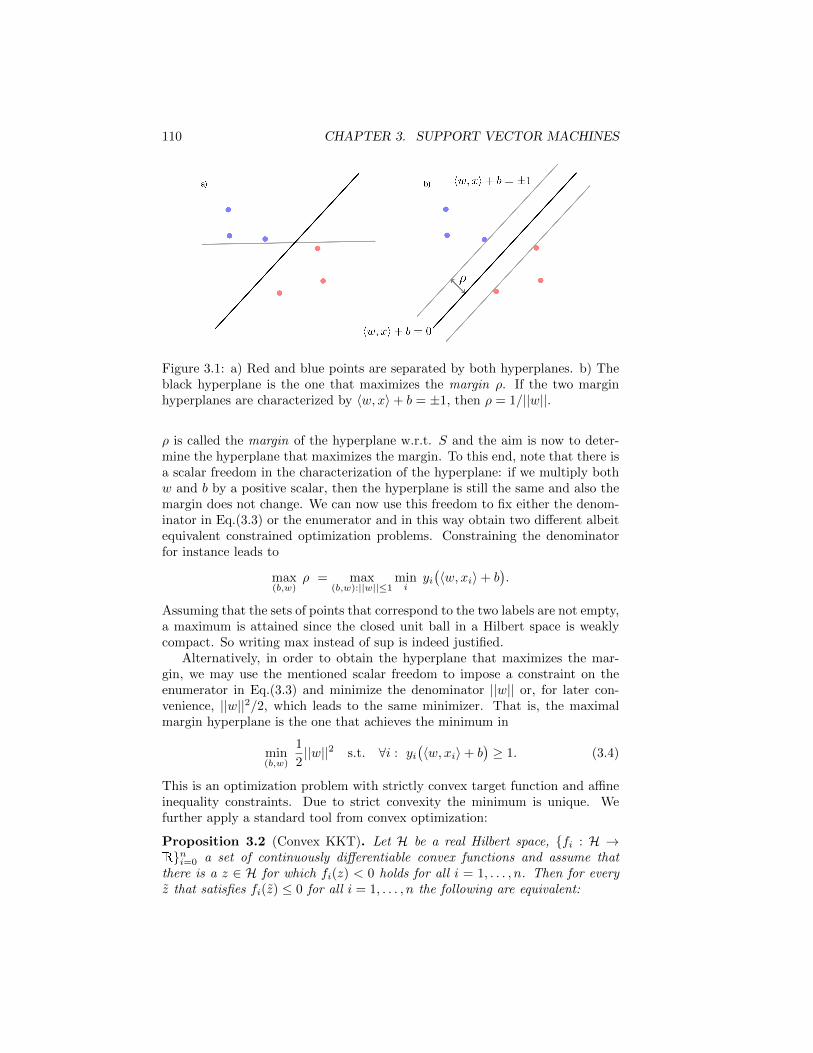
110 CHAPTER 3. SUPPORT VECTOR MACHINES
Figure 3.1: a) Red and blue points are separated by both hyperplanes. b) Theblack hyperplane is the one that maximizes the margin ρ. If the two marginhyperplanes are characterized by 〈w, x〉+ b = ±1, then ρ = 1/||w||.
ρ is called the margin of the hyperplane w.r.t. S and the aim is now to deter-mine the hyperplane that maximizes the margin. To this end, note that there isa scalar freedom in the characterization of the hyperplane: if we multiply bothw and b by a positive scalar, then the hyperplane is still the same and also themargin does not change. We can now use this freedom to fix either the denom-inator in Eq.(3.3) or the enumerator and in this way obtain two different albeitequivalent constrained optimization problems. Constraining the denominatorfor instance leads to
max(b,w)
ρ = max(b,w):||w||≤1
mini
yi(〈w, xi〉+ b
).
Assuming that the sets of points that correspond to the two labels are not empty,a maximum is attained since the closed unit ball in a Hilbert space is weaklycompact. So writing max instead of sup is indeed justified.
Alternatively, in order to obtain the hyperplane that maximizes the mar-gin, we may use the mentioned scalar freedom to impose a constraint on theenumerator in Eq.(3.3) and minimize the denominator ||w|| or, for later con-venience, ||w||2/2, which leads to the same minimizer. That is, the maximalmargin hyperplane is the one that achieves the minimum in
min(b,w)
1
2||w||2 s.t. ∀i : yi
(〈w, xi〉+ b
)≥ 1. (3.4)
This is an optimization problem with strictly convex target function and affineinequality constraints. Due to strict convexity the minimum is unique. Wefurther apply a standard tool from convex optimization:
Proposition 3.2 (Convex KKT). Let H be a real Hilbert space, fi : H →Rni=0 a set of continuously differentiable convex functions and assume thatthere is a z ∈ H for which fi(z) < 0 holds for all i = 1, . . . , n. Then for everyz that satisfies fi(z) ≤ 0 for all i = 1, . . . , n the following are equivalent:
3.1. LINEAR MAXIMAL MARGIN SEPARATORS 111
1. f0(z) = minz∈Hf0(z) | fi(z) ≤ 0 ∀i = 1, . . . , n.
2. There exist λi ≤ 0 so that
∇f0(z) =
n∑
i=1
λi∇fi(z) and (3.5)
λifi(z) = 0 ∀i = 1, . . . , n. (3.6)
Applying this to the optimization problem in Eq.(3.4) leads to the follow-ing crucial insight: if w corresponds to the maximal margin hyperplane, thenEq.(3.5) implies w =
∑ni=1 yiλixi. That is, the minimizing w is a linear combi-
nation of the training data points xi. In addition, Eq.(3.6), which in our casereads λi
[1 − yi
(〈w, xi〉 + b
)]= 0, implies that only those xi’s contribute for
which the i’th constraint is active. This means yi(〈w, xi〉 + b
)= 1 so that the
corresponding xi is sitting on one of the two margin hyperplanes. These xi’sare called support vectors.
Non-separable case Now we drop the assumption that the data is exactlylinearly separable. However, we still seek a predictor that is given in terms ofa hyperplane and that in some sense still has maximal margin. The differenceto the foregoing discussion is that we now allow for outliers that may either beon the wrong side of the hyperplane or inside the margin. In order to formalizethis, one introduces slack variables ξi ≥ 0 that measure the extent to whichthe i’th constraint is violated. In addition, one penalizes these violations in theobject function. This leads to the optimization problem
min(b,w,ξ)
λ
2||w||2 +
1
n
n∑
i=1
ξi
s.t. yi(〈w, xi〉+ b
)≥ 1− ξi ∧ ξi ≥ 0 ∀i = 1, . . . n,
(3.7)
where λ > 0 is a free parameter that can be used to adjust the strength of thepenalty. There is some arbitrariness in how one penalizes large ξ. In Eq.(3.7)we have essentially chosen the l1-norm of ξ. Another common choice would bethe l2-norm.
The optimization problem in Eq.(3.7) can be written as ERM problem w.r.t.the so-called hinge loss Lhinge : R×R→ R+ that is defined as
Lhinge(y, y′) := max0, 1− yy′.
The hinge loss provides an upper bound on the usually taken loss functionfor binary classification in the sense that if y ∈ −1, 1, then 1y 6=sgn(h(x)) ≤Lhinge(y, h(x)). Other noticeable properties are that y′ 7→ Lhinge(y, y
′) is convexand w 7→ Lhinge(y, 〈w, x〉+ b) is ||x||-Lipschitz.
112 CHAPTER 3. SUPPORT VECTOR MACHINES
Figure 3.2: a) Outliers (points that are either inside the margin corridor, or onthe wrong side) are penalized using slack variable ξi. b) The hinge loss (blue),plotted for the case y = 1, is a convex upper bound for the 0-1-loss (red) thatis usually used for binary classification.
The optimization problem in Eq.(3.7) can now be written as
min(b,w)
λ
2||w||2 +
1
n
n∑
i=1
max
0, 1− yi(〈w, xi〉+ b
)
= min(b,w)
λ
2||w||2 + Rhinge(h), (3.8)
where h(x) := 〈w, x〉 + b. Note that Eq.(3.8) is a regularized ERM problemwithout additional constraints.
Theorem 3.1: Representer theorem
Let H be a Hilbert space, g : R → R non-decreasing, f : Rn → R,x1, . . . , xn ⊆ H, Hx := spanxini=1 and F : H → R, F (w) := g(||w||) +f(〈w, x1〉, . . . , 〈w, xn〉). Then
infw∈H
F (w) = infw∈Hx
F (w) (3.9)
and if g is strictly increasing, then every minimizer of the l.h.s. of Eq.(3.9)is an element of Hx.
Proof. We use that H = Hx⊕H⊥x and that every w ∈ H admits a correspondingdecomposition of the form w = wx + v where wx ∈ Hx and v ∈ H⊥x . Then〈w, xi〉 = 〈wx, xi〉 holds for all i and from Pythagoras we obtain
g(||w||) = g(√||wx||2 + ||v||2
)≥ g(||wx||).
Here, strict inequality holds if g is strictly increasing and w 6= wx. Hence, theclaims follow by replacing w by wx in the argument of F .
3.2. POSITIVE SEMIDEFINITE KERNELS 113
3.2 Positive semidefinite kernels
Definition 3.3 (PSD kernel). Let K ∈ R,C and X be an arbitrary set. Amap K : X ×X → K is called positive semidefinite kernel (PSD kernel) iff forall n ∈ N and all x ∈ Xn the n × n matrix G with entries Gij := K(xi, xj) ispositive semidefinite.
The terminology varies considerably throughout the literature. PSD kernelsalso run under the names positive definite kernels, positive definite symmetrickernels, kernel functions or just kernels. Recall that a matrix G is positivesemidefinite iff G is hermitian, i.e., Gij = Gji, and G has only non-negativeeigenvalues. The latter condition can be replaced with
∀α ∈ Kn :
n∑
i,j=1
αiαjGij ≥ 0. (3.10)
Theorem 3.2: PSD kernels and feature maps
Let X be any set, K ∈ R,C and K : X ×X → K.
1. K is a PSD kernel, if there is an inner product space H and a mapφ : X → H so that
K(x, y) = 〈φ(x), φ(y)〉 ∀x, y ∈ X. (3.11)
2. Conversely, if K is a PSD kernel, then there exists a Hilbert spaceH and a map φ : H → K so that Eq.(3.11) holds.
Note: the map φ is often called feature map and the inner product space H thefeature space.
Proof. 1. If K is of the form in Eq.(3.11), then for all α ∈ Kn and x ∈ Xn wehave
∑ni,j=1 αiαj〈φ(xj), φ(xi)〉 = 〈Φ,Φ〉 ≥ 0 where Φ :=
∑ni=1 αiφ(xi). Her-
miticity of the respective matrix follows from hermiticity of the inner product.2. Assume K to be a PSD kernel and define
H0 := spankx : X → K | ∃x ∈ X : kx(y) = K(x, y)
(3.12)
the space of all finiteK-linear combination of functions of the form y 7→ K(x, y).We aim at equipping this space with an inner product. For two arbitrary ele-ments of H0 given by f(y) :=
∑i αiK(xi, y) and g(y) :=
∑j βjK(xj , y) define
〈f, g〉 :=∑
i,j
αiβjK(xi, xj)
=∑
i
αig(xi) =∑
j
βjf(xj),
114 CHAPTER 3. SUPPORT VECTOR MACHINES
where the second line shows that the definition is independent of the particulardecomposition of f or g. So 〈·, ·〉 is a well defined hermitian sesquilinear formon H0. Moreover, since K is a PSD kernel, we have 〈g, g〉 ≥ 0 for all g ∈ H0.Hence, the Cauchy Schwarz inequality holds. Applying it to
f(y) =∑
i
αiK(xi, y) = 〈f, ky〉, (3.13)
we obtain |f(y)|2 = |〈f, ky〉|2 ≤ 〈ky, ky〉〈f, f〉. This shows that 〈f, f〉 = 0 impliesf = 0 and thus 〈·, ·〉 is indeed an inner product. Note that if we apply Eq.(3.13)to f = kx, we obtain
kx(y) = K(x, y) = 〈kx, ky〉. (3.14)
So if we denote by H the completion of the inner product space H0 and defineφ : X → H so that φ(x) is the isometric embedding of kx into H, then Eq.(3.14)implies K(x, y) = 〈φ(x), φ(y)〉.
Proposition 3.4 (Building new PSD kernels). Let K ∈ R,C, K1,K2, . . .PSD kernels on a set X and f ∈ KX . Then
1. K(x, y) := f(x)f(y) is a PSD kernel.
2. K(x, y) := λK1(x, y) is a PSD kernel for all λ ≥ 0.
3. K(x, y) := K1(x, y) +K2(x, y) is a PSD kernel.
4. K(x, y) := limn→∞Kn(x, y) is a PSD kernel, if the limits exist in K.
5. K(x, y) := K1(x, y)K2(x, y) is a PSD kernel.
Proof. In all cases hermiticity is rather obvious, so we only have a look at posi-
tive semidefiniteness. 1. K is PSD since∑ni=1 αiαjf(xi)f(xj) =
∣∣∑ni=1 αif(xi)
∣∣2is always positive. 2. and 3. are elementary consequences of the definition. 4. isimplied by the closedness of the set of PSD matrices, or more explicitly by pos-itivity of
∑mi=1 αiαjK(x, y) = limn→∞
∑mi=1 αiαjKn(x, y) as a limit of positive
numbers. 5. follows from the fact the set of PSD matrices is closed under takingelement wise products (called Schur products or Hadamard products).
With these tools at hand, many kernels can easily be shown to be PSD.Some of the most common examples are:
Example 3.1 (Polynomial kernels). On X = Rd any polynomial in 〈x, y〉 withnon-negative coefficients is a PSD kernel as a consequence of 2., 3. and 5.in Prop. 3.4 together with the fact that (x, y) → 〈x, y〉 is (the paradigm of)a PSD kernel. In particular, K(x, y) := (1 + 〈x, y〉)2 is a PSD kernel. OnR2 this can be obtained from the feature map φ(x) : R2 → R6, φ(x) :=(x2
1, x22,√
2x1x2,√
2x1,√
2x2, 1). Like in this example, all polynomial kernelshave corresponding finite dimensional feature spaces.
Example 3.2 (Exponential kernels). For any γ > 0, K(x, y) := exp[γ〈x, y〉] is aPSD kernel on X = Rd since it is a limit of polynomial kernels so that 4. inProp. 3.4 applies.
3.3. REPRODUCING KERNEL HILBERT SPACES 115
Example 3.3 (Gaussian kernels). The Gaussian kernel K(x, y) := exp[− γ
2 ||x−y||2]
with the Euclidean norm is a PSD kernel on X = Rd for all γ > 0. To seethis write
exp[− γ
2||x− y||2
]= exp[−γ||x||2/2] exp[−γ||y||2/2]︸ ︷︷ ︸
f(x)f(y)
exp[γ〈x, y〉]
and apply 1. and 5. of Prop. 3.4.
Example 3.4 (Binomial kernels). On X := x ∈ Rd | ||x||2 < 1 K(x, y) :=(1 − 〈x, y〉
)−pis a PSD kernel for any p > 0. This follows again from the
previous proposition by noting that for t ∈ (−1, 1) the binomial series (1−t)−p =∑∞n=0(−1)n
(−pn
)tn has positive coefficients (−1)n
(−pn
)= (−1)n
∏ni=1(1−p−i)/i.
We will see in Sec.3.4 that, whereas polynomial kernels have finite dimen-sional feature spaces, exponential, Gaussian and binomial kernels require infinitedimensional feature space.
3.3 Reproducing kernel Hilbert spaces
For a given PSD kernel, the corresponding feature map and feature space are notunique. However, there is a canonical choice for the feature space, a so-calledreproducing kernel Hilbert space.
Definition 3.5 (Reproducing kernel Hilbert space). Let X be a set, K ∈ R,Cand H ⊆ KX a K-Hilbert space of functions on X with addition (f + g)(x) :=f(x) + g(x) and multiplication (λf)(x) := λf(x). H is called a reproducingkernel Hilbert space (RKHS) on X iff for all x ∈ H the linear functional δx :H → K, δx(f) := f(x) is bounded (i.e., supf∈H\0 |f(x)|/||f || <∞).
Note: Since δx is linear, boundedness is equivalent to continuity. That is,the defining property of a RKHS is that evaluation of its functions at arbitrarypoints is continuous w.r.t. varying the function.
Example 3.5. If X is countable, then l2(X) := f ∈ KX |∑x∈X |f(x)|2 <∞
equipped with 〈f, g〉 :=∑x∈X f(x)g(x) is a RKHS since for all x ∈ X we have
|f(x)| ≤(∑
y∈X |f(y)|2)1/2
= ||f ||. Hence, δx is bounded.
Example 3.6. L2([0, 1]) is not a RKHS. Since its elements are equivalence classesof functions that differ on sets of measure zero, f(x) is not defined. Even ifwe restrict to the subspace of continuous functions, where f(x) is defined, itsmagnitude is not bounded by imposing ||f || ≤ 1. So δx is not bounded.
Since l2(N) and L2([0, 1]) are isomorphic, these two examples show thatHilbert space isomorphisms do not necessarily preserve the RKHS property.
A crucial consequence of the continuity of δx in any RKHS is that one caninvoke the Riesz representation theorem. This states that every continuouslinear functional on a Hilbert space can be represented as inner product with aunique vector. In particular, if H is a RKHS, then for every x ∈ X there is a
116 CHAPTER 3. SUPPORT VECTOR MACHINES
kx ∈ H so that f(x) = 〈f, kx〉 for all f ∈ H. Since inner products are alwayscontinuous, this can be regarded as equivalent characterization of a RKHS. As kxis an element of H and therefore a function on X, we can define K : X×X → K,K(x, y) := kx(y). K is called the reproducing kernel of the RKHSH. Using thatkx(y) can itself be expressed in terms of an inner product with some elementky, we obtain
K(x, y) = 〈kx, ky〉. (3.15)
Before we relate reproducing kernel Hilbert spaces to PSD kernels, let us mentionsome elementary properties:
Proposition 3.6. Let H ⊆ KX be a RKHS with reproducing kernel K andkx(y) = K(x, y). Let f, fn ∈ H and δx(f) := f(x) for x ∈ X, f ∈ H. Then
1. For all x ∈ H we have ||δx||2 = K(x, x).
2. limn→∞ ||fn − f || = 0 ⇒ ∀x ∈ X : limn→∞ fn(x) = f(x).
3. spankx | x ∈ X is dense in H.
Proof. 1. follows with f(x) = 〈f, kx〉 from
||δx||2 = supf∈H\0
|〈kx, f〉|2
||f ||2= ||kx||2 = 〈kx, kx〉 = K(x, x), (3.16)
where the second equality is the one of the Cauchy Schwarz inequality. Similarly,also 2. is obtained from Cauchy Schwarz by noting that
∣∣fn(x)− f(x)∣∣ =
∣∣〈kx, fn − f〉∣∣ ≤ ||kx|| ||fn − f || → 0.
For 3. it suffices to show that there is no non-zero element that is orthogonalto the considered span. Indeed, suppose f ∈ H is orthogonal to all kx, then forall x ∈ X we have that 0 = 〈f, kx〉 = f(x), which means f = 0.
Theorem 3.3: RKHS and PSD kernels
1. If H is a RKHS on X, then its reproducing kernel K : X ×X → K
is a PSD kernel.
2. Conversely, if K : X × X → K is a PSD kernel, then there is aunique RKHS H ⊆ KX so that K is its reproducing kernel.
Proof. 1. If K is the reproducing kernel of a RKHS H, then by Eq.(3.15) andthe properties of the inner product:
∀x, y ∈ X : K(x, y) = 〈kx, ky〉 = 〈ky, kx〉 = K(y, x) andn∑
i,j=1
αiαjK(xi, xj) =
n∑
i,j=1
αiαj〈kxi , kxj 〉 =∣∣∣∣∣∣n∑
i=1
αikxi
∣∣∣∣∣∣2
≥ 0.
3.4. UNIVERSAL AND STRICTLY POSITIVE KERNELS 117
2. (sketch) The construction of the sought RKHS is the one in the proof ofThm.3.2. Eqs.(3.13,3.14) show that K fulfills the requirement of a reproducingkernel on H0. A more careful consideration shows that the relevant propertiesare indeed preserved when going from H0 to its completion H.
To address uniqueness suppose H1 and H2 are two RKHS with reproducingkernel K. Following 3. in Prop.3.6 the space H0 = spankx|x ∈ X is densein both H1 and H2. Moreover, if f ∈ H0 with f(x) =
∑i αikxi , then ||f ||2l =∑
i,j αiαjK(xi, xj) for l = 1, 2. Hence, the norms || · ||1 and || · ||2 coincide onH0.
Suppose f ∈ H1. Then there are fn ∈ H0 so that ||fn−f ||1 → 0. As (fn)n∈Nis Cauchy inH1 it is also Cauchy inH2 and therefore there exist a g ∈ H2 so that||fn − g||2 → 0. According to 2. in Prop.3.6 we have f(x) = limn→∞ fn(x) =g(x) for all x ∈ X. Hence, f = g ∈ H2 and consequently H1 = H2. Sincethe norms, and by polarization also the inner products, coincide on a densesubspace, the do so on its completion.
3.4 Universal and strictly positive kernels
Definition 3.7 (Universal kernels). A PSD kernel K : X×X → K on a metricspace X is called universal iff for all ε > 0, all compact subsets X ⊆ X andevery continuous function f : X → K there exists g ∈ spankx : X → K | ∃x ∈X : kx(y) = K(x, y) so that
∣∣g(x)− f(x)∣∣ ≤ ε ∀x ∈ X. (3.17)
Note that if φ : X → H is a feature map corresponding to K, then Eq.(3.17)means that there exists a w ∈ H so that
∣∣〈w, φ(x)〉 − f(x)∣∣ ≤ ε ∀x ∈ X. (3.18)
Corollary 3.8 (Universal kernels separate all compact subsets). Let φ : X → Hbe a feature map of a universal PSD kernel on a metric space X. For any pairof disjoint compact subsets A+, A− ⊆ X there exists a w ∈ H so that for allx ∈ A+ ∪A−:
sgn〈w, φ(x)〉 =
+1, x ∈ A+
−1, x ∈ A−(3.19)
Proof. As the distance between A+ and A− is non-zero, we can extend thefunction A+ ∪A− 3 x 7→ 1x∈A+
− 1x∈A− to a continuous function f on X. Byuniversality there exists a w ∈ H for each ε ∈ (0, 1) so that |〈w, φ(x)〉−f(x)| ≤ εfor all x ∈ A+ ∪A−. Hence,
〈w, φ(x)〉≥ 1− ε, x ∈ A+
≤ ε− 1, x ∈ A−(3.20)
Note that in this case the sets are separated with margin (1− ε)/||w||.
118 CHAPTER 3. SUPPORT VECTOR MACHINES
Theorem 3.4: Taylor criterion for universality
Let f(z) :=∑∞n=0 anz
n be a power series with radius of convergence r ∈(0,∞] and X := x ∈ Rd | ||x||2 <
√r. If an > 0 for all n, then
K : X ×X → R, K(x, y) := f(〈x, y〉) is a universal PSD kernel.
Proof. First note that K is well defined since |〈x, y〉| ≤ ||x||2||y||2 < r. Usingmultinomial expansion we can write
K(x, y) =
∞∑
n=0
an
(d∑
k=1
xkyk
)n=
∞∑
n=0
an∑
k1 + · · ·+ kd = nk1, . . . , kd ≥ 0
n!
k1! · · · kd!
d∏
i=1
(xiyi)ki
=∑
k1,...,kd≥0
ak1+...+kd
(k1 + . . .+ kd)!
k1! · · · kd!︸ ︷︷ ︸=:ck
d∏
i=1
xkii
d∏
j=1
ykjj . (3.21)
This enables us to introduce a feature map φ : X → l2(Nd0
)as φk(x) :=
√ck∏di=1 x
kii for k ∈ Nd0 so that K(x, y) = 〈φ(x), φ(y)〉. Since all an’s are
strictly positive, the same holds true for all ck’s. Consequently, spanφkk∈Nd0is the space of all polynomials and by the Stone-Weierstrass theorem dense inthe set of continuous functions on compact domains. The claim then followsfrom the observation that every finite linear combination of functions of theform x 7→ φk(x) can be regarded as an inner product 〈w, φ(x)〉 for some vectorw. Since the latter has only finitely many non-zero components, it is indeed anelement of l2
(Nd0
).
Corollary 3.9. On X = Rd the following are universal PSD kernels:
1. Exponential kernel: K(x, y) := exp(γ〈x, y〉
), γ > 0.
2. Gaussian kernel: K(x, y) := exp(− γ
2 ||x− y||22
), γ > 0.
Proof. Universality of the exponential kernel follows directly from Thm.3.4 withan = τn/n!. This in turn can be used to prove universality of the Gaussiankernel: if φ : X → H is a feature map of the exponential kernel, then φ :x 7→ φ(x)/||φ(x)|| is a feature map of the Gaussian kernel. Now take anycompact subset X ⊆ X and define c := supx∈X ||φ(x)||−1. By universality ofthe exponential kernel, for every continuous function f : X → R there is aw ∈ H so that ∣∣∣f(x)||φ(x)|| − 〈w, φ(x)〉
∣∣∣ ≤ ε
c∀x ∈ X.
Dividing by ||φ(x)|| and taking the supremum over x ∈ X on the resulting r.h.s.leads to
∣∣f(x)− 〈w, φ(x)〉∣∣ ≤ ε for all x ∈ X.
Proposition 3.10 (Strict positivity of universal kernels). Let K : X ×X → K
be a universal PSD kernel on a metric space X. Then K is strictly positivedefinite, i.e., for all n ∈ N, every set of n distinct points x1, . . . , xn ∈ X andall α ∈ Kn\0 we have
∑ni,j=1 αiαjK(xi, xj) > 0.
3.4. UNIVERSAL AND STRICTLY POSITIVE KERNELS 119
Proof. Assume K is not strictly positive definite, i.e.,∑ni,j=1 αiαjK(xi, xj) = 0
for some α ∈ Kn\0 and x ∈ Xn. Expressing this in terms of the canonicalfeature map φ : X → H, where H is the corresponding RKHS, we obtainthat
∑ni=1 αiφ(xi) = 0 since it has vanishing norm. Now for an arbitrary
function induced by the kernel via g(x) :=∑mj=1 βj〈φ(x), φ(yj)〉 we obtain∑n
i=1 αig(xi) =∑i,j αiβj〈φ(xi), φ(yj)〉 = 0. Hence, the set of functions induced
by the kernel cannot be dense in the set of continuous functions on the compactset X :=
⋃ni=1xi since any continuous function f for which
∑ni=1 αif(xi) 6= 0
cannot be approximated to arbitrary accuracy. So K cannot be universal.
Proposition 3.11 (Properties of strictly positive definite kernels). Let K :X × X → K be a strictly positive definite kernel on a set X. That is, for alln ∈ N, every set of n distinct points x1, . . . , xn ∈ X and all α ∈ Kn\0 wehave
∑ni,j=1 αiαjK(xi, xj) > 0 and K(xi, xj) = K(xj , xi). Then:
1. Every corresponding feature space is infinite dimensional.
2. Every corresponding feature map is injective.
3. If A+, A− are disjoint finite subsets of X and φ : X → H is any featuremap corresponding to K, then there is a w ∈ H and b ∈ R so that
Re〈w, φ(x)〉> b, if x ∈ A+
< b, if x ∈ A−(3.22)
Proof. 1. If φ : X → H is any feature map for K and d := dim(H) < ∞, thenany set of n > d vectors φ(xi)ni=1 is linearly dependent. Therefore, there isan α ∈ Kn\0 so that 0 =
∑ni,j=1 αiαj〈φ(xi), φ(xj)〉 =
∑ni,j=1 αiαjK(xi, xj),
which implies that K is not strictly positive definite.2. As argued in the proof of 1., if x 6= y, then φ(x) and φ(y) have to be
linearly independent. So in particular φ is injective.3. The central observation is again linear independence of the set of vectors
φ(x)x∈A+∪A− . If we define C± := convφ(x)x∈A± as the convex hulls of theimages of the sets A+ and A− under φ, then linear independence implies that C+
and C− are disjoint sets. Moreover, they are closed and bounded convex subsetscontained in finite dimensional subspace so that we can invoke the geometricHahn-Banach separation theorem for compact convex sets to arrive at Eq.(3.22).
Theorem 3.5: Translation invariant kernels
Let µ be a finite non-negative Borel measure on X := Rd and denote byχ ∈ C(X) its Fourier transform
χ(x) :=
∫
X
e−ix·zdµ(z). (3.23)
Then K(x, y) := χ(x − y) is a PSD kernel on X. Moreover, K is strictly

120 CHAPTER 3. SUPPORT VECTOR MACHINES
positive definite, if the complement of the largest open set U ⊆ X thatsatisfies µ(U) = 0 has non-zero Lebesgue measure.
Proof. Consider distinct points x1, . . . , xn ∈ X and α ∈ Cn\0. Then
n∑
k,j=1
αkαjK(xk, xj) =
n∑
k,j=1
αkαj
∫
X
e−i(xk−xj)·zdµ(z)
=
∫
X
∣∣∣∣∣n∑
k=1
αke−ixk·z
∣∣∣∣∣
2
︸ ︷︷ ︸=:ψ(z)
dµ(z) ≥ 0. (3.24)
So K is a PSD kernel. Moreover, strict inequality holds in Eq.(3.24) unless thesupport of µ is contained in the zero set ψ−1(0). However, ψ−1(0) alwayshas zero Lebesgue measure so that every µ whose support has non-zero Lebesguemeasure leads to a strictly positive definite kernel.
3.5 Rademacher bounds
... to be completed ...
Theorem 3.6: Rademacher bound for bounded inner products
Let ρ, r > 0 be positive constants, x1, . . . , xn points in a real Hilbert spaceH so that ||xi|| ≤ r for all i and G := g : H → R | g(z) = 〈z, w〉, ||w||−1 ≥ρ. With Gij := 〈xi, xj〉 the empirical Rademacher complexity of G w.r.t.x1, . . . xn satisfies
R(G) ≤ tr[G]1/2
nρ≤ r
ρ√n. (3.25)
Proof. The first inequality follows from
R(G) =1
nEσ
[sup
||w||≤1/ρ
⟨ n∑
i=1
σixi, w⟩]
≤ 1
nρEσ
∣∣∣∣∣∣n∑
i=1
σixi
∣∣∣∣∣∣ ≤ 1
nρ
[Eσ
∣∣∣∣∣∣n∑
i=1
σixi
∣∣∣∣∣∣2]1/2
=1
nρ
Eσ
n∑
i,j=1
σiσj〈xi, xj〉
1/2
=1
nρ
[n∑
i=1
〈xi, xi〉
]1/2
.
Here the first inequality is implied by Cauchy-Schwarz and the second by Jensen’sinequality (applied to the concave square root function). The last step in the
3.5. RADEMACHER BOUNDS 121
chain follows from the fact that if i 6= j, then Eσ[σiσj ] = Eσ[σi] Eσ[σj ] = 0since the Rademacher variables are independent and uniform.
The second inequality in Eq.(3.25) uses in addition that∑ni=1〈xi, xi〉 ≤
nr2.

122 CHAPTER 3. SUPPORT VECTOR MACHINES

Bibliography
[1] Amiran Ambroladze, Emilio Parrado-Hernandez, and John Shawe-Taylor.Complexity of pattern classes and the Lipschitz property. Theor. Comput.Sci., 382(3):232–246, 2007.
[2] Peter L Bartlett, Vitaly Maiorov, and Ron Meir. Almost Linear VC-Dimension Bounds for Piecewise Polynomial Networks. Neural Comput.,10(8):2159–2173, 1998.
[3] P.L. Bartlett, P.M. Long, and R.C. Williamson. Fat-shattering and thelearnability of real-valued functions. J. Comput. Syst. Sci., 52(3):434–452,1996.
[4] Eric B. Baum and David Haussler. What Size Net Gives Valid Generaliza-tion? Neural Comput., 1(1):151–160, 1989.
[5] Shai Ben-David, N. Cesa-Bianchi, D. Haussler, and P. Long. Characteriza-tion of learnability for classes of n-valued functions. J. Comput. Syst. Sci.,50:74–86, 1995.
[6] Shai Ben-David and Michael Lindenbaum. Lcalization vs. Identification ofSemi-Algebraic Sets. Mach. Learn., 32:207–224, 1998.
[7] Anselm Blumer, Andrzej Ehrenfeucht, David Haussler, and Manfred K.Warmuth. Learnability and the Vapnik-Chervonenkis dimension. J. ACM,36(4):929–965, 1989.
[8] Ralph P. Boas and Harold P. Boas. A Primer of Real Functions. CambridgeUniversity Press, 1996.
[9] Amit Daniely, Sivan Sabato, Shai Ben-David, and Shai Shalev-Shwartz.Multiclass Learnability and the ERM principle.
[10] Christian J.J. Despres. The Vapnik-Chervonenkis dimension of norm onRd. 2014.
[11] R. M. Dudley. Balls in Rk do not cut all subsets of k + 2 points. Adv.Math. (N. Y)., 31(3):306–308, 1979.
123
124 BIBLIOGRAPHY
[12] Paul W Goldberg and Mark R Jerrum. Bounding the Vapnik-Chervonenkisdimension of concept classes parameterized by real numbers. Mach. Learn.,18(2):131–148, 1995.
[13] Nick Harvey, Chris Liaw, and Abbas Mehrabian. Nearly-tight VC-dimension bounds for piecewise linear neural networks.
[14] W. Hoeffding. Probability inequalities for sums of bounded random vari-ables. J. Am. Stat. Assoc., 58(301):13–30, 1963.
[15] Jean Jacod and Philip Protter. Probability Essentials. Springer Berlin /Heidelberg, 2 edition, 2004.
[16] Marek Karpinski and Angus Macintyre. Polynomial Bounds for VC Di-mension of Sigmoidal and General Pfaffian Neural Networks. J. Comput.Syst. Sci., 54(1):169–176, 1997.
[17] Pascal Koiran and Eduardo D Sontag. Neural Networks with QuadraticVC Dimension. J. Comput. Syst. Sci., 54(1):190–198, 1997.
[18] W G Maass. Neural networks with superlinear VC dimension. NeuralComput., 6:877–884, 1994.
[19] Colin McDiarmid. On the method of bounded differences, 1989.
[20] Allan Pinkus. Approximation theory of the MLP model in neural networks.Acta Numer., 8:143, 1999.
[21] A. Sakurai. Tight bounds for the VC-dimension of piecewise polynomialnetworks. Adv. Neural Inf. Process. Syst., 11:323–329, 1998.
[22] Shai Shalev-Shwartz, Ohad Shamir, Nathan Srebro, and Karthik Sridha-ran. Learnability, Stability and Uniform Convergence. J. Mach. Learn.Res., 11:2635–2670, 2010.