math208: discrete mathematicsarts-sciences.und.edu/math/_files/docs/courses/208text/... · ·...
TRANSCRIPT
U N D M AT H E M AT I C S
M AT H 2 0 8 :D I S C R E T EM AT H E M AT I C S
D E PA R T M E N T O F M AT H E M AT I C S
T H E U N I V E R S I T Y O F N O R T H D A K O TA
Copyright © 2017 UND Mathematics
published by department of mathematics
the university of north dakota
http://arts-sciences.und.edu/math//
Copyright © 2005, 2006, 2007, 2008, 2009, 2014, 2015, 2016, 2017 University of North Dakota Mathematics
Department
Permission is granted to copy, distribute and/or modify this document under the terms of the GNU Free
Documentation License, Version 1.2 or any later version published by the Free Software Foundation; with
no Invariant Sections, no Front-Cover Texts, and no Back-Cover Texts. A copy of the license is included in
the section entitled "GNU Free Documentation License".
Second corrected edition, Second printing: December 2017
Contents
1 Logical Connectives and Compound Propositions 25
1.1 Propositions 25
1.2 Negation: not 26
1.3 Conjunction: and 27
1.4 Disjunction: or 27
1.5 Logical Implication and Biconditional 28
1.5.1 Implication: If . . . , then . . . 28
1.5.2 Biconditional: . . . if and only if . . . 29
1.6 Truth table construction 29
1.7 Translating to propositional forms 30
1.8 Bit strings 30
1.9 Exercises 32
2 Logical Equivalence 35
2.1 Logical Equvalence 35
2.2 Tautologies and Contradictions 36
2.3 Related If . . . , then . . . propositions 36
2.4 Fundamental equivalences 36
4
2.5 Disjunctive normal form 37
2.6 Proving equivalences 38
2.7 Exercises 40
3 Predicates and Quantifiers 41
3.1 Predicates 41
3.2 Instantiation and Quantification 42
3.3 Translating to symbolic form 43
3.4 Quantification and basic laws of logic 44
3.5 Negating quantified statements 45
3.6 Exercises 46
4 Rules of Inference 49
4.1 Valid propositional arguments 50
4.2 Fallacies 53
4.3 Arguments with quantifiers 53
4.4 Exercises 55
5 Sets: Basic Definitions 57
5.1 Specifying sets 57
5.1.1 Roster method 57
5.1.2 Set-builder notation 58
5.2 Special standard sets 58
5.3 Empty and universal sets 58
5.4 Subset and equality relations 59
5
5.5 Cardinality 60
5.6 Power set 60
5.7 Exercises 61
6 Set Operations 63
6.1 Intersection 63
6.2 Venn diagrams 63
6.3 Union 63
6.4 Symmetric difference 64
6.5 Complement 64
6.6 Ordered lists 64
6.7 Cartesian product 65
6.8 Laws of set theory 65
6.9 Proving set identities 67
6.10 Bit string operations 67
6.11 Exercises 68
7 Styles of Proof 69
7.1 Direct proof 69
7.2 Indirect proof 72
7.3 Proof by contradiction 72
7.4 Proof by cases 74
7.5 Existence proof 75
7.6 Using a counterexample to disprove a statement 75
7.7 Exercises 77
6
8 Relations 79
8.1 Relations 79
8.2 Specifying a relation 80
8.2.1 By ordered pairs 80
8.2.2 By graph 80
8.2.3 By digraph: domain=codomain 81
8.2.4 By 0-1 matrix 81
8.3 Set operations with relations 82
8.3.1 Subset relation using matrices 82
8.4 Special relation operations 83
8.4.1 Inverse of a relation 83
8.4.2 Composition of relations 83
8.4.3 Composition with matrices: Boolean product 84
8.5 Exercises 85
9 Properties of Relations 87
9.1 Reflexive 87
9.2 Irreflexive 88
9.3 Symmetric 88
9.4 Antisymmetric 89
9.5 Transitive 89
9.6 Examples 89
9.7 Exercises 91
10 Equivalence Relations 93
10.1 Equvialence relation 94
7
10.2 Equivalence class of a relation 94
10.3 Examples 95
10.4 Partitions 97
10.5 Digraph of an equivalence relation 97
10.6 Matrix representation of an equivalence relation 97
10.7 Exercises 99
11 Functions and Their Properties 101
11.1 Definition of function 102
11.2 Functions with discrete domain and codomain 102
11.2.1 Representions by 0-1 matrix or bipartite graph 103
11.3 Special properties 103
11.3.1 One-to-one (injective) 104
11.3.2 Onto (surjective) 105
11.3.3 Bijective 105
11.4 Composition of functions 106
11.5 Invertible discrete functions 106
11.6 Characteristic functions 108
11.7 Exercises 109
12 Special Functions 111
12.1 Floor and ceiling functions 111
12.2 Fractional part 111
12.3 Integral part 112
12.4 Power functions 112
8
12.5 Exponential functions 112
12.6 Logarithmic functions 113
12.7 Laws of logarithms 113
12.8 Exercises 115
13 Sequences and Summation 117
13.1 Specifying sequences 117
13.1.1 Defining a Sequence With a Formula 118
13.1.2 Defining a Sequence by Suggestion 118
13.2 Arithmetic sequences 119
13.3 Geometric sequences 120
13.4 Summation notation 120
13.5 Formulas for arithmetic and geometric summations 122
13.6 Exercises 124
14 Recursively Defined Sequences 125
14.1 Closed form formulas 126
14.1.1 Pattern recognition 126
14.1.2 The Fibonacci Sequence 126
14.1.3 The Sequence of Factorials 127
14.2 Arithmetic sequences by recursion 128
14.3 Exercises 129
15 Recursively Defined Sets 131
15.1 Recursive definitions of sets 131
15.2 Sets of strings 133
15.3 Exercises 135
9
16 Mathematical Induction 137
16.1 Mathematical induction 138
16.2 The principle of mathematical induction 139
16.3 Proofs by induction 140
16.4 Examples 142
16.5 Second principle of mathematical induction 144
16.6 Exercises 148
17 Algorithms 149
17.1 Properties of an algorithm 149
17.2 Non-algorithms 150
17.3 Linear search algorithm 150
17.4 Binary search algorithm 151
17.5 Presenting algorithms 151
17.6 Examples 153
17.7 Exercises 156
18 Algorithm Efficiency 159
18.1 Comparing algorithms 160
18.2 Exercises 163
19 The Growth of Functions 165
19.1 Common efficiency functions 166
19.2 Big-oh notation 166
19.3 Examples 167
19.4 Exercises 168
10
20 The Integers 169
20.1 Integer operations 169
20.2 Order properties 172
20.3 Exercises 173
21 The divides Relation and Primes 175
21.1 Properties of divides 175
21.2 Prime numbers 176
21.3 The division algorithm for integers 177
21.4 Exercises 179
22 GCD’s and the Euclidean Algorithm 181
22.1 Euclidean algorithm 182
22.2 Efficiency of the Euclidean algorithm 183
22.3 The Euclidean algorithm in quotient/remainder form 184
22.4 Exercises 186
23 GCD’s Reprised 187
23.1 The gcd(a, b) as a linear combination of a and b 187
23.2 Back-solving to express gcd(a, b) as a linear combination 188
23.3 Extended Euclidean Algorithm 189
23.4 General Linear Combinations for gcd(a, b) 192
23.5 Exercises 194
11
24 The Fundamental Theorem of Arithmetic 195
24.1 Prime divisors 195
24.2 Proving the Fundamental Theorem 196
24.3 Number of positive divisors of n 197
24.4 Exercises 198
25 Linear Diophantine Equations 199
25.1 Diophantine equations 200
25.2 Solutions and gcd(a, b) 200
25.3 Finding all solutions 201
25.4 Examples 202
25.5 Exercises 204
26 Modular Arithmetic 205
26.1 The modulo m equivalence relation 206
26.2 Equivalence classes modulo m 207
26.3 Modular arithmetic 207
26.4 Solving congruence equations 209
26.5 Exercises 211
27 Integers in Other Bases 213
27.1 Converting to and from base-10 213
27.2 Converting between non-decimal bases 215
27.3 Computer science bases: 2, 8, and 16 216
27.4 Exercises 217
12
28 The Two Fundamental Counting Principles 219
28.1 The sum rule 219
28.1.1 Counting two independent tasks 220
28.1.2 Extended sum rule 221
28.1.3 Sum rule and the logical or 221
28.2 The product rule 221
28.2.1 Counting two sequential tasks: logical and 222
28.2.2 Extended product rule 222
28.2.3 Counting by subtraction: Good = Total − Bad 223
28.3 Using both the sum and product rules 224
28.4 Answer form←→ solution method 226
28.5 Exercises 227
29 Permutations and Combinations 229
29.1 Permutations 229
29.2 Combinations 231
29.3 Exercises 233
30 The Binomial Theorem and Pascal’s Triangle 235
30.1 Combinatorial proof 235
30.1.1 Constructing combinatorial proofs 236
30.2 Pascal’s Triangle 238
30.3 The Binomial Theorem 239
30.4 Exercises 241
13
31 Inclusion-Exclusion Counting 243
31.1 Inclusion-Exclusion principle 243
31.2 Extended inclusion-exclustion principle 245
31.3 Inclusion-exclusion with the Good=Total-Bad trick 247
31.4 Exercises 249
32 The Pigeonhole Principle 251
32.1 General pigeonhole principle 252
32.2 Examples 252
32.3 Exercises 254
33 Tougher Counting Problems 255
33.1 The Basic Donut Shop Problem 256
33.2 The More Realistic Donut Shop Problem 257
33.3 The Real Donut Shop Problem 257
33.4 Problems with order and some repetition 259
33.5 The six fundamental counting problems 260
33.6 Exercises 261
34 Counting Using Recurrence Relations 263
34.1 Recursive counting method 263
34.2 Examples 266
34.3 General rules for finding recursive solutions 269
34.4 Exercises 271
14
35 Solutions to Recurrence Relations 273
35.1 Solving a recursion by conjecture 273
35.2 Solving a recursion by unfolding 274
35.3 Exercises 276
36 The Method of Characteristic Roots 277
36.1 Homogeneous, constant coefficient recursions 277
36.1.1 Basic example of the method 278
36.1.2 Initial steps: the characteristic equation and its roots 280
36.2 Repeated characteristic roots. 280
36.3 The method of characteristic roots more formally 281
36.4 The method for repeated roots 283
36.5 The general case 284
36.6 Exercises 286
37 Solving Nonhomogeneous Recurrences 287
37.1 Steps to solve nonhomogeneous recurrence relations 287
37.2 Examples 289
37.3 Exercises 292
38 Graphs 293
38.1 Some Graph Terminology 293
38.1.1 Representing a graph in a computer 294
15
38.2 An Historical Interlude: The origin of graph theory 296
38.3 The First Theorem of Graph Theory 304
38.4 A Brief Catalog of Special Graphs 305
38.5 Graph isomorphisms 307
38.6 Walks 309
38.6.1 Eulerian trails and circuits 311
38.6.2 Hamiltonian cycles 311
38.6.3 Some facts about eulerian and hamiltonian graphs 312
38.7 Trees 314
38.8 Exercises 316
A Answers 319
B GNU Free Documentation License 321
1. APPLICABILITY AND DEFINITIONS 322
2. VERBATIM COPYING 324
3. COPYING IN QUANTITY 324
4. MODIFICATIONS 325
5. COMBINING DOCUMENTS 328
6. COLLECTIONS OF DOCUMENTS 328
7. AGGREGATION WITH INDEPENDENT WORKS 329
8. TRANSLATION 329
9. TERMINATION 330
10. FUTURE REVISIONS OF THIS LICENSE 330
11. RELICENSING 331
ADDENDUM: How to use this License for your documents 331

List of Figures
4.1 A logical argument 52
6.1 Venn diagram for A ∩ B 63
6.2 Venn diagram for A ∪ B 64
6.3 Venn diagram for A⊕ B 64
6.4 Venn diagram for A− B 64
6.5 Venn diagram for A = U − A 64
8.1 Example bipartite graph 81
8.2 Example digraph 81
8.3 Composing relations: R ◦ S 84
11.1 Graph of y = x2102
11.2 A function in 0-1 matrix form 103
12.1 Floor function 111
12.2 Fractional part function 112
12.3 Integral part function 112
12.4 2x and log2(x) functions 113
16.1 4× 5 chessboard 143
16.2 23 × 23 chessboard 143
16.3 Divided 23 × 23 chessboard 144
16.4 23 × 23 board with domino 144
30.1 Pascal’s Triangle 238
30.2 Pascal’s Triangle (numeric) 238
31.1 A ∪ B = (A− B) ∪ B 243
18
38.1 Nonisomorphic grades with the same degree sequences. 308
38.2 Isomorphic graphs 308
38.3 More Isomorphic graphs 309
38.4 Walks, trails, and paths 310
38.5 Tree for exercise 38.6 318
List of Tables
1.1 Logical Negation 27
1.2 Logical Conjunction 27
1.3 Logical or and xor 28
1.4 Logical Implication 28
1.5 Logical biconditional 29
1.6 Truth table for (p ∧ q)→ r 30
2.1 Prove p→ q ≡ ¬p ∨ q 36
2.2 Logical Equivalences 37
4.1 Basic rules of inference 51
4.2 Proof of an argument 52
4.3 Quantification rules 54
6.1 Laws of Set Theory 66
11.1 A simple function 102
19.1 Problem size vs. CPU time used 165
19.2 Common efficiency functions for small values of n 166
19.3 Efficiency functions where n = 1000000 166
23.1 i: 6567(si) + 987(ti) = ri, qi−1 190
23.2 gcd(107653, 22869) 191
33.1 Basic counting problems 255
33.2 Six counting problems 260
37.1 Particular solution patterns 288

List of Algorithms
17.1 Linear search (repeat/until). (A B indicates a comment follows.) 152
17.2 Linear search (for loop) 152
17.3 Calculate bm/nc 153
17.4 Calculate bm/nc (again) 154
17.5 Make change 155
18.1 Maximum list value 162

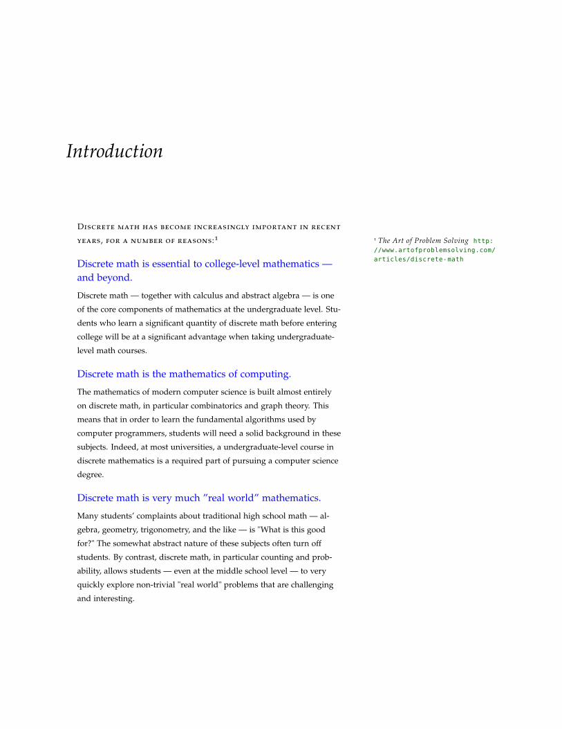
Introduction
Discrete math has become increasingly important in recent
years, for a number of reasons:1 1 The Art of Problem Solving http:
//www.artofproblemsolving.com/
articles/discrete-mathDiscrete math is essential to college-level mathematics —and beyond.
Discrete math — together with calculus and abstract algebra — is one
of the core components of mathematics at the undergraduate level. Stu-
dents who learn a significant quantity of discrete math before entering
college will be at a significant advantage when taking undergraduate-
level math courses.
Discrete math is the mathematics of computing.
The mathematics of modern computer science is built almost entirely
on discrete math, in particular combinatorics and graph theory. This
means that in order to learn the fundamental algorithms used by
computer programmers, students will need a solid background in these
subjects. Indeed, at most universities, a undergraduate-level course in
discrete mathematics is a required part of pursuing a computer science
degree.
Discrete math is very much ”real world” mathematics.
Many students’ complaints about traditional high school math — al-
gebra, geometry, trigonometry, and the like — is "What is this good
for?" The somewhat abstract nature of these subjects often turn off
students. By contrast, discrete math, in particular counting and prob-
ability, allows students — even at the middle school level — to very
quickly explore non-trivial "real world" problems that are challenging
and interesting.
24 math208: discrete mathematics
Discrete math shows up on most middle and high schoolmath contests.
Prominent math competitions such as MATHCOUNTS (at the middle
school level) and the American Mathematics Competitions (at the high
school level) feature discrete math questions as a significant portion
of their contests. On harder high school contests, such as the AIME,
the quantity of discrete math is even larger. Students that do not have
a discrete math background will be at a significant disadvantage in
these contests. In fact, one prominent MATHCOUNTS coach tells us
that he spends nearly 50% of his preparation time with his students
covering counting and probability topics, because of their importance
in MATHCOUNTS contests.
Discrete math teaches mathematical reasoning and prooftechniques.
Algebra is often taught as a series of formulas and algorithms for
students to memorize (for example, the quadratic formula, solving
systems of linear equations by substitution, etc.), and geometry is often
taught as a series of ”definition-theorem-proof” exercises that are often
done by rote (for example, the infamous ”two-column proof”). While
undoubtedly the subject matter being taught is important, the material
(as least at the introductory level) does not lend itself to a great deal of
creative mathematical thinking. By contrast, with discrete mathematics,
students will be thinking flexibly and creatively right out of the box.
There are relatively few formulas to memorize; rather, there are a
number of fundamental concepts to be mastered and applied in many
different ways.
Discrete math is fun.
Many students, especially bright and motivated students, find algebra,
geometry, and even calculus dull and uninspiring. Rarely is this the
case with most discrete math topics. When we ask students what their
favorite topic is, most respond either ”combinatorics” or ”number
theory.” (When we ask them what their least favorite topic is, the
overwhelming response is ”geometry.”) Simply put, most students find
discrete math more fun than algebra or geometry.
1
Logical Connectives and Compound Propositions
Logic is concerned with forms of reasoning. Since reasoning
is involved in most intellectual activities, logic is relevant to a broad
range of pursuits. The study of logic is essential for students of com-
puter science. It is also very valuable for mathematics students, and
others who make use of mathematical proofs, for instance, linguistics
students. In the process of reasoning one makes inferences. In an in-
ference one uses a collection of statements, the premises, in order to
justify another statement, the conclusion. The most reliable types of
inferences are deductive inferences, in which the conclusion must be
true if the premises are. Recall elementary geometry: Assuming that
the postulates are true, we prove that other statements, such as the
Pythagorean Theorem, must also be true. Geometric proofs, and other
mathematical proofs, typically use many deductive inferences. (Robert
L. Causey)1 1 www.cs.utexas.edu/~rlc/whylog.htm
1.1 Propositions
The basic objects in logic are propositions. A proposition is a state-
ment which is either true (T) or false (F) but not both. For example in
the language of mathematics p : 3 + 3 = 6 is a true proposition while
q : 2 + 3 = 6 is a false proposition. What do you want for lunch? is a
question, not a proposition. Likewise Get lost! is a command, not a
proposition. The sentence There are exactly 1087 + 3 stars in the universe
is a proposition, despite the fact that no one knows its truth value.
Here are two, more subtle, examples:
26 math208: discrete mathematics
(1) He is more than three feet tall is not a proposition since, until we are
told to whom he refers, the statement cannot be assigned a truth
value. The mathematical sentence x + 3 = 7 is not a proposition
for the same reason. In general, sentences containing variables are
not propositions unless some information is supplied about the
variables. More about that later however. Sometimes a little common sense is
required. For example It is raining is a
proposition, but its truth value is not
constant, and may be arguable. That
is, someone might say It is not raining,
it is just drizzling, or Do you mean on
Venus? Feel free to ignore these sorts of
annoyances.
(2) This sentence is false is not a proposition. It seems to be both true
and false. In fact if is T then it says it is F and if it is F then it says
it is T. It is a good idea to avoid sentences that refer to themselves.
Simple propositions, such as It is raining, and The streets are wet,
can be combined to create more complicated propositions such as It
is raining and the streets are not wet. These sorts of involved proposi-
tions are called compound propositions. Compound propositions are
built up from simple propositions using a number of connectives to
join or modify the simple propositions. In the last example, the con-
nectives are and which joins the two clauses, and not, which modifies
the second clause.
It is important to keep in mind that since a compound proposition
is, after all, a proposition, it must be classifiable as either true or false.
That is, it must be possible to assign a truth value to any compound
proposition. There are mutually agreed upon rules to allow the deter-
mination of exactly when a compound proposition is true and when
it is false. Luckily these rules jive nicely with common sense (with
one small exception), so they are easy to remember and understand.
1.2 Negation: not
The simplest logical connective is negation. In normal English sen-
tences, this connective is indicated by appropriately inserting not in
the statement, by preceding the statement with it is not the case that, or
for mathematical statements, by using a slanted slash. For example,
if p is the proposition 2 + 3 = 4, then the negation of p is denoted
by the symbol ¬p and it is the proposition 2 + 3 6= 4. In this case,
p is false and ¬p is true. If p is It is raining, then ¬p is It is not rain-
ing or even the stilted sounding It is not the case that it is raining. The
logical connectives and compound propositions 27
negation of a proposition p is the proposition whose truth value is
the opposite of p in all cases. The behavior of ¬p can be exhibited in
a truth table. In each row of the truth table we list a possible truth
value of p and the corresponding truth value of ¬p.
p ¬p
T F
F TTable 1.1: Logical Negation
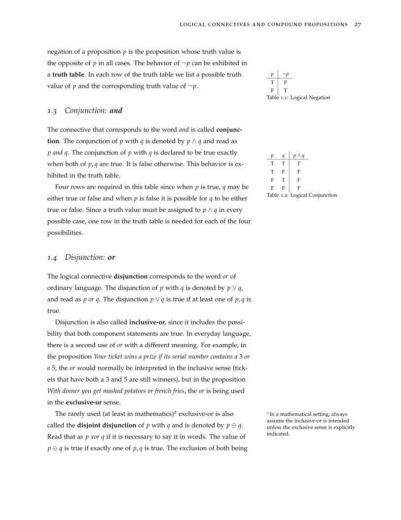
1.3 Conjunction: and
The connective that corresponds to the word and is called conjunc-
tion. The conjunction of p with q is denoted by p ∧ q and read as
p and q. The conjunction of p with q is declared to be true exactly
when both of p, q are true. It is false otherwise. This behavior is ex-
hibited in the truth table.
p q p ∧ q
T T T
T F F
F T F
F F FTable 1.2: Logical Conjunction
Four rows are required in this table since when p is true, q may be
either true or false and when p is false it is possible for q to be either
true or false. Since a truth value must be assigned to p ∧ q in every
possible case, one row in the truth table is needed for each of the four
possibilities.
1.4 Disjunction: or
The logical connective disjunction corresponds to the word or of
ordinary language. The disjunction of p with q is denoted by p ∨ q,
and read as p or q. The disjunction p ∨ q is true if at least one of p, q is
true.
Disjunction is also called inclusive-or, since it includes the possi-
bility that both component statements are true. In everyday language,
there is a second use of or with a different meaning. For example, in
the proposition Your ticket wins a prize if its serial number contains a 3 or
a 5, the or would normally be interpreted in the inclusive sense (tick-
ets that have both a 3 and 5 are still winners), but in the proposition
With dinner you get mashed potatoes or french fries, the or is being used
in the exclusive-or sense.
The rarely used (at least in mathematics)2 exclusive-or is also 2 In a mathematical setting, alwaysassume the inclusive-or is intendedunless the exclusive sense is explicitlyindicated.
called the disjoint disjunction of p with q and is denoted by p ⊕ q.
Read that as p xor q if it is necessary to say it in words. The value of
p⊕ q is true if exactly one of p, q is true. The exclusion of both being
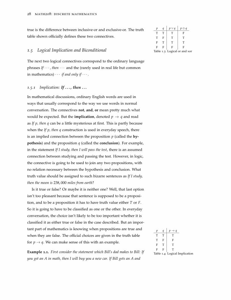
28 math208: discrete mathematics
true is the difference between inclusive-or and exclusive-or. The truth
table shown officially defines these two connectives.
p q p ∨ q p⊕ q
T T T F
T F T T
F T T T
F F F FTable 1.3: Logical or and xor1.5 Logical Implication and Biconditional
The next two logical connectives correspond to the ordinary language
phrases If · · · , then · · · and the (rarely used in real life but common
in mathematics) · · · if and only if · · · .
1.5.1 Implication: If . . . , then . . .
In mathematical discussions, ordinary English words are used in
ways that usually correspond to the way we use words in normal
conversation. The connectives not, and, or mean pretty much what
would be expected. But the implication, denoted p → q and read
as If p, then q can be a little mysterious at first. This is partly because
when the If p, then q construction is used in everyday speech, there
is an implied connection between the proposition p (called the hy-
pothesis) and the proposition q (called the conclusion). For example,
in the statement If I study, then I will pass the test, there is an assumed
connection between studying and passing the test. However, in logic,
the connective is going to be used to join any two propositions, with
no relation necessary between the hypothesis and conclusion. What
truth value should be assigned to such bizarre sentences as If I study,
then the moon is 238, 000 miles from earth?
Is it true or false? Or maybe it is neither one? Well, that last option
isn’t too pleasant because that sentence is supposed to be a proposi-
tion, and to be a proposition it has to have truth value either T or F.
So it is going to have to be classified as one or the other. In everyday
conversation, the choice isn’t likely to be too important whether it is
classified it as either true or false in the case described. But an impor-
tant part of mathematics is knowing when propositions are true and
when they are false. The official choices are given in the truth table
for p→ q. We can make sense of this with an example.
p q p→ q
T T T
T F F
F T T
F F TTable 1.4: Logical ImplicationExample 1.1. First consider the statement which Bill’s dad makes to Bill: If
you get an A in math, then I will buy you a new car. If Bill gets an A and
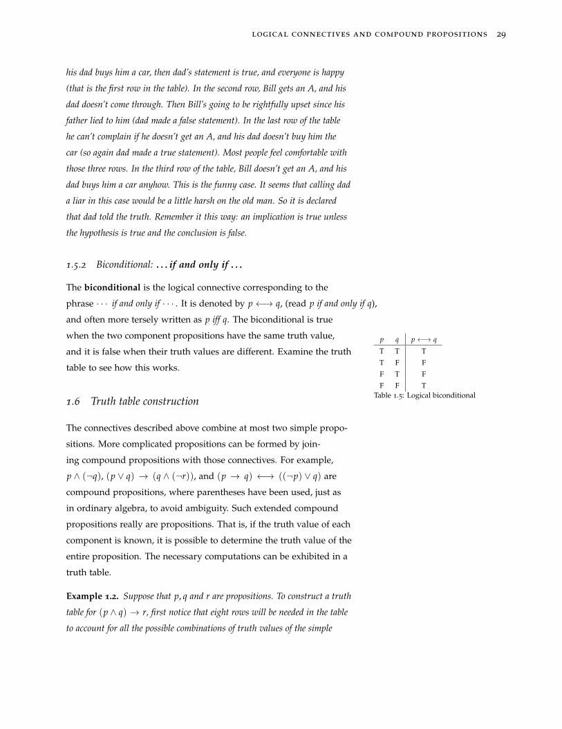
logical connectives and compound propositions 29
his dad buys him a car, then dad’s statement is true, and everyone is happy
(that is the first row in the table). In the second row, Bill gets an A, and his
dad doesn’t come through. Then Bill’s going to be rightfully upset since his
father lied to him (dad made a false statement). In the last row of the table
he can’t complain if he doesn’t get an A, and his dad doesn’t buy him the
car (so again dad made a true statement). Most people feel comfortable with
those three rows. In the third row of the table, Bill doesn’t get an A, and his
dad buys him a car anyhow. This is the funny case. It seems that calling dad
a liar in this case would be a little harsh on the old man. So it is declared
that dad told the truth. Remember it this way: an implication is true unless
the hypothesis is true and the conclusion is false.
1.5.2 Biconditional: . . . if and only if . . .
The biconditional is the logical connective corresponding to the
phrase · · · if and only if · · · . It is denoted by p←→ q, (read p if and only if q),
and often more tersely written as p iff q. The biconditional is true
when the two component propositions have the same truth value,
and it is false when their truth values are different. Examine the truth
table to see how this works.
p q p←→ q
T T T
T F F
F T F
F F TTable 1.5: Logical biconditional
1.6 Truth table construction
The connectives described above combine at most two simple propo-
sitions. More complicated propositions can be formed by join-
ing compound propositions with those connectives. For example,
p ∧ (¬q), (p ∨ q) → (q ∧ (¬r)), and (p → q) ←→ ((¬p) ∨ q) are
compound propositions, where parentheses have been used, just as
in ordinary algebra, to avoid ambiguity. Such extended compound
propositions really are propositions. That is, if the truth value of each
component is known, it is possible to determine the truth value of the
entire proposition. The necessary computations can be exhibited in a
truth table.
Example 1.2. Suppose that p, q and r are propositions. To construct a truth
table for (p ∧ q) → r, first notice that eight rows will be needed in the table
to account for all the possible combinations of truth values of the simple
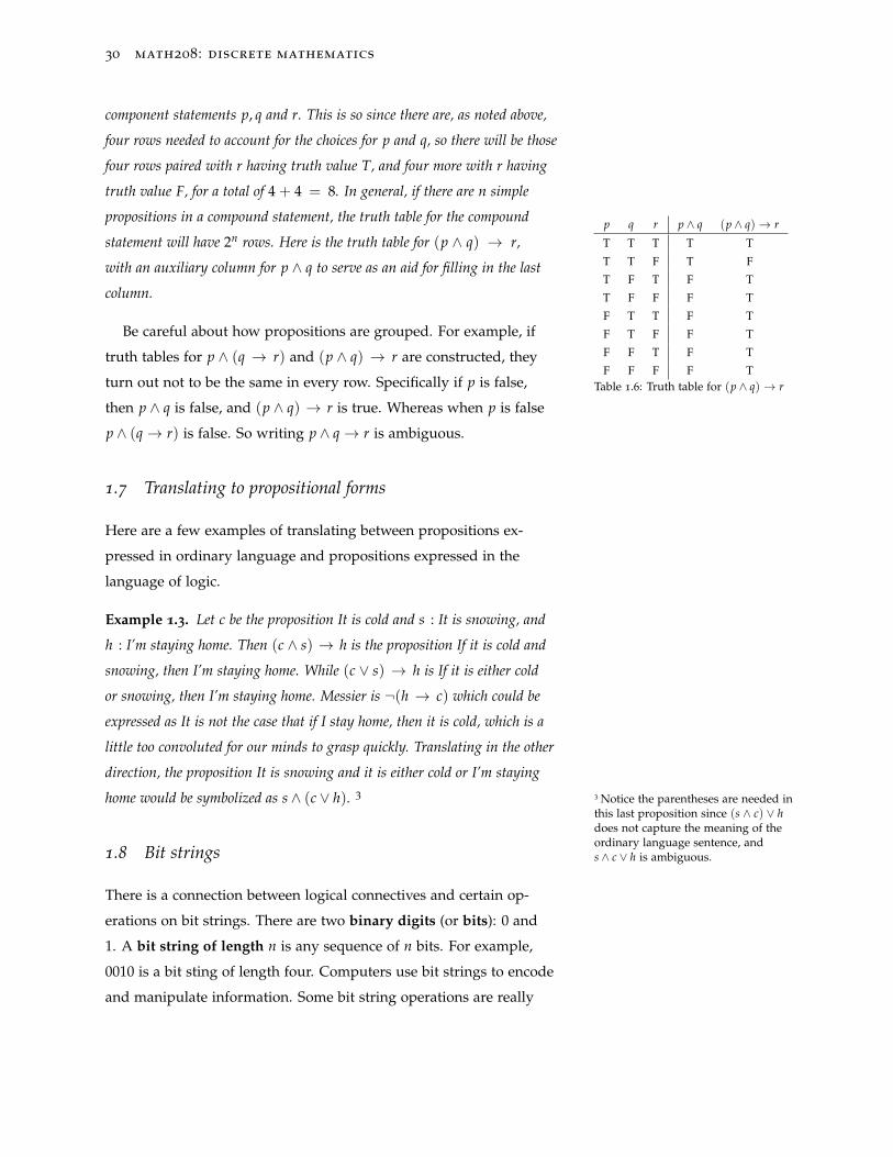
30 math208: discrete mathematics
component statements p, q and r. This is so since there are, as noted above,
four rows needed to account for the choices for p and q, so there will be those
four rows paired with r having truth value T, and four more with r having
truth value F, for a total of 4 + 4 = 8. In general, if there are n simple
propositions in a compound statement, the truth table for the compound
statement will have 2n rows. Here is the truth table for (p ∧ q) → r,
with an auxiliary column for p ∧ q to serve as an aid for filling in the last
column.
p q r p ∧ q (p ∧ q)→ r
T T T T T
T T F T F
T F T F T
T F F F T
F T T F T
F T F F T
F F T F T
F F F F TTable 1.6: Truth table for (p ∧ q)→ r
Be careful about how propositions are grouped. For example, if
truth tables for p ∧ (q → r) and (p ∧ q) → r are constructed, they
turn out not to be the same in every row. Specifically if p is false,
then p ∧ q is false, and (p ∧ q) → r is true. Whereas when p is false
p ∧ (q→ r) is false. So writing p ∧ q→ r is ambiguous.
1.7 Translating to propositional forms
Here are a few examples of translating between propositions ex-
pressed in ordinary language and propositions expressed in the
language of logic.
Example 1.3. Let c be the proposition It is cold and s : It is snowing, and
h : I’m staying home. Then (c ∧ s) → h is the proposition If it is cold and
snowing, then I’m staying home. While (c ∨ s) → h is If it is either cold
or snowing, then I’m staying home. Messier is ¬(h → c) which could be
expressed as It is not the case that if I stay home, then it is cold, which is a
little too convoluted for our minds to grasp quickly. Translating in the other
direction, the proposition It is snowing and it is either cold or I’m staying
home would be symbolized as s ∧ (c ∨ h). 3 3 Notice the parentheses are needed inthis last proposition since (s ∧ c) ∨ hdoes not capture the meaning of theordinary language sentence, ands ∧ c ∨ h is ambiguous.1.8 Bit strings
There is a connection between logical connectives and certain op-
erations on bit strings. There are two binary digits (or bits): 0 and
1. A bit string of length n is any sequence of n bits. For example,
0010 is a bit sting of length four. Computers use bit strings to encode
and manipulate information. Some bit string operations are really
logical connectives and compound propositions 31
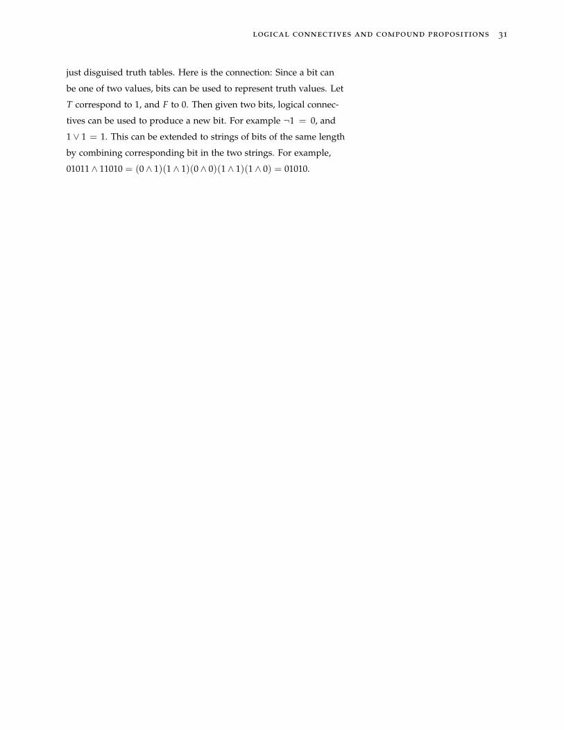
just disguised truth tables. Here is the connection: Since a bit can
be one of two values, bits can be used to represent truth values. Let
T correspond to 1, and F to 0. Then given two bits, logical connec-
tives can be used to produce a new bit. For example ¬1 = 0, and
1 ∨ 1 = 1. This can be extended to strings of bits of the same length
by combining corresponding bit in the two strings. For example,
01011∧ 11010 = (0∧ 1)(1∧ 1)(0∧ 0)(1∧ 1)(1∧ 0) = 01010.
32 math208: discrete mathematics
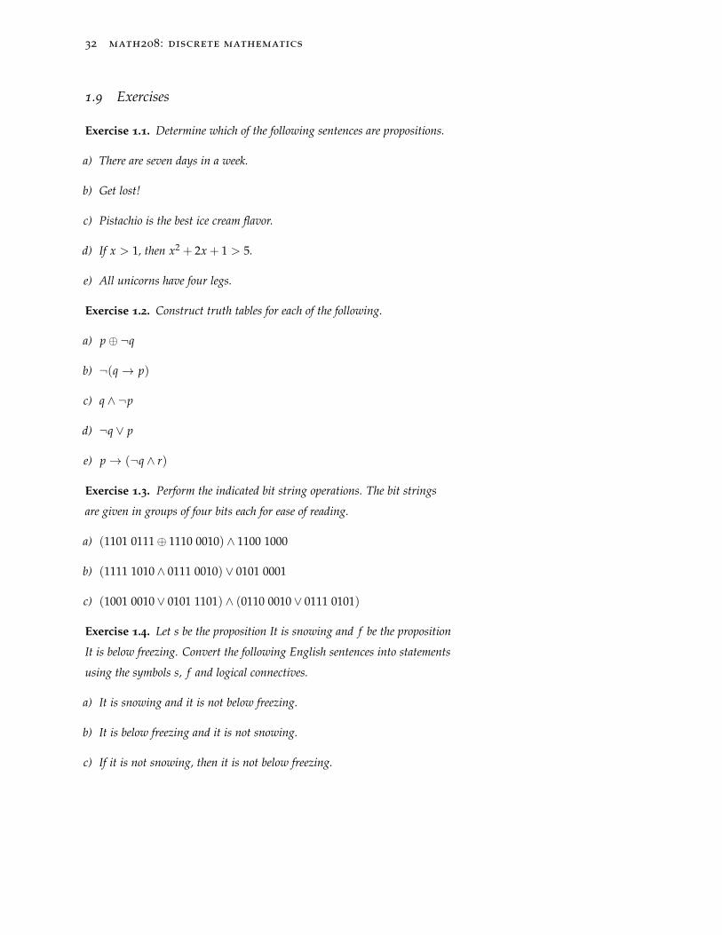
1.9 Exercises
Exercise 1.1. Determine which of the following sentences are propositions.
a) There are seven days in a week.
b) Get lost!
c) Pistachio is the best ice cream flavor.
d) If x > 1, then x2 + 2x + 1 > 5.
e) All unicorns have four legs.
Exercise 1.2. Construct truth tables for each of the following.
a) p⊕¬q
b) ¬(q→ p)
c) q ∧ ¬p
d) ¬q ∨ p
e) p→ (¬q ∧ r)
Exercise 1.3. Perform the indicated bit string operations. The bit strings
are given in groups of four bits each for ease of reading.
a) (1101 0111⊕ 1110 0010) ∧ 1100 1000
b) (1111 1010∧ 0111 0010) ∨ 0101 0001
c) (1001 0010∨ 0101 1101) ∧ (0110 0010∨ 0111 0101)
Exercise 1.4. Let s be the proposition It is snowing and f be the proposition
It is below freezing. Convert the following English sentences into statements
using the symbols s, f and logical connectives.
a) It is snowing and it is not below freezing.
b) It is below freezing and it is not snowing.
c) If it is not snowing, then it is not below freezing.
logical connectives and compound propositions 33
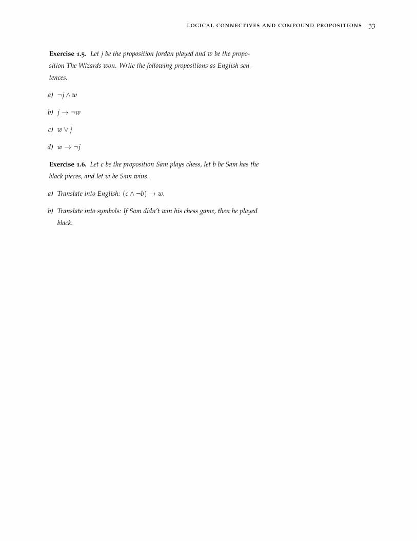
Exercise 1.5. Let j be the proposition Jordan played and w be the propo-
sition The Wizards won. Write the following propositions as English sen-
tences.
a) ¬j ∧ w
b) j→ ¬w
c) w ∨ j
d) w→ ¬j
Exercise 1.6. Let c be the proposition Sam plays chess, let b be Sam has the
black pieces, and let w be Sam wins.
a) Translate into English: (c ∧ ¬b)→ w.
b) Translate into symbols: If Sam didn’t win his chess game, then he played
black.

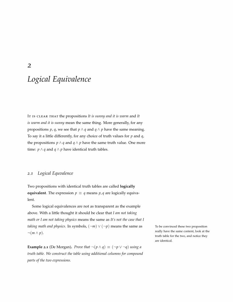
2
Logical Equivalence
It is clear that the propositions It is sunny and it is warm and It
is warm and it is sunny mean the same thing. More generally, for any
propositions p, q, we see that p ∧ q and q ∧ p have the same meaning.
To say it a little differently, for any choice of truth values for p and q,
the propositions p ∧ q and q ∧ p have the same truth value. One more
time: p ∧ q and q ∧ p have identical truth tables.
2.1 Logical Equvalence
Two propositions with identical truth tables are called logically
equivalent. The expression p ≡ q means p, q are logically equiva-
lent.
Some logical equivalences are not as transparent as the example
above. With a little thought it should be clear that I am not taking
math or I am not taking physics means the same as It’s not the case that I
taking math and physics. In symbols, (¬m) ∨ (¬p) means the same as To be convinced these two proposition
really have the same content, look at the
truth table for the two, and notice they
are identical.
¬(m ∧ p).
Example 2.1 (De Morgan). Prove that ¬(p ∧ q) ≡ (¬p ∨ ¬q) using a
truth table. We construct the table using additional columns for compound
parts of the two expressions.
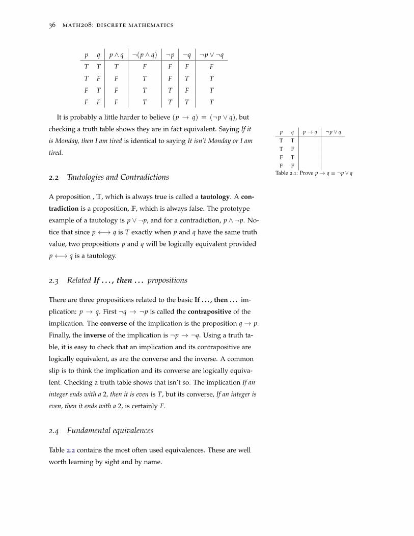
36 math208: discrete mathematics
p q p ∧ q ¬(p ∧ q) ¬p ¬q ¬p ∨ ¬q
T T T F F F F
T F F T F T T
F T F T T F T
F F F T T T T
It is probably a little harder to believe (p → q) ≡ (¬p ∨ q), but
checking a truth table shows they are in fact equivalent. Saying If it
is Monday, then I am tired is identical to saying It isn’t Monday or I am
tired.
p q p→ q ¬p ∨ q
T T
T F
F T
F FTable 2.1: Prove p→ q ≡ ¬p ∨ q2.2 Tautologies and Contradictions
A proposition , T, which is always true is called a tautology. A con-
tradiction is a proposition, F, which is always false. The prototype
example of a tautology is p ∨ ¬p, and for a contradiction, p ∧ ¬p. No-
tice that since p ←→ q is T exactly when p and q have the same truth
value, two propositions p and q will be logically equivalent provided
p←→ q is a tautology.
2.3 Related If . . . , then . . . propositions
There are three propositions related to the basic If . . . , then . . . im-
plication: p → q. First ¬q → ¬p is called the contrapositive of the
implication. The converse of the implication is the proposition q→ p.
Finally, the inverse of the implication is ¬p → ¬q. Using a truth ta-
ble, it is easy to check that an implication and its contrapositive are
logically equivalent, as are the converse and the inverse. A common
slip is to think the implication and its converse are logically equiva-
lent. Checking a truth table shows that isn’t so. The implication If an
integer ends with a 2, then it is even is T, but its converse, If an integer is
even, then it ends with a 2, is certainly F.
2.4 Fundamental equivalences
Table 2.2 contains the most often used equivalences. These are well
worth learning by sight and by name.
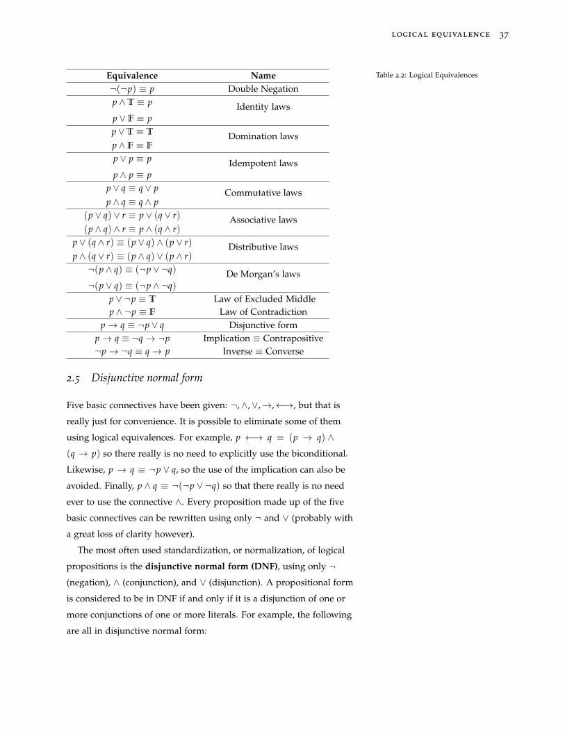
logical equivalence 37
Equivalence Name¬(¬p) ≡ p Double Negationp ∧T ≡ p Identity lawsp ∨F ≡ pp ∨T ≡ T Domination lawsp ∧F ≡ F
p ∨ p ≡ p Idempotent lawsp ∧ p ≡ p
p ∨ q ≡ q ∨ p Commutative lawsp ∧ q ≡ q ∧ p
(p ∨ q) ∨ r ≡ p ∨ (q ∨ r) Associative laws(p ∧ q) ∧ r ≡ p ∧ (q ∧ r)
p ∨ (q ∧ r) ≡ (p ∨ q) ∧ (p ∨ r) Distributive lawsp ∧ (q ∨ r) ≡ (p ∧ q) ∨ (p ∧ r)¬(p ∧ q) ≡ (¬p ∨ ¬q) De Morgan’s laws¬(p ∨ q) ≡ (¬p ∧ ¬q)
p ∨ ¬p ≡ T Law of Excluded Middlep ∧ ¬p ≡ F Law of Contradiction
p→ q ≡ ¬p ∨ q Disjunctive formp→ q ≡ ¬q→ ¬p Implication ≡ Contrapositive¬p→ ¬q ≡ q→ p Inverse ≡ Converse
Table 2.2: Logical Equivalences
2.5 Disjunctive normal form
Five basic connectives have been given: ¬,∧,∨,→,←→, but that is
really just for convenience. It is possible to eliminate some of them
using logical equivalences. For example, p ←→ q ≡ (p → q) ∧(q → p) so there really is no need to explicitly use the biconditional.
Likewise, p → q ≡ ¬p ∨ q, so the use of the implication can also be
avoided. Finally, p ∧ q ≡ ¬(¬p ∨ ¬q) so that there really is no need
ever to use the connective ∧. Every proposition made up of the five
basic connectives can be rewritten using only ¬ and ∨ (probably with
a great loss of clarity however).
The most often used standardization, or normalization, of logical
propositions is the disjunctive normal form (DNF), using only ¬(negation), ∧ (conjunction), and ∨ (disjunction). A propositional form
is considered to be in DNF if and only if it is a disjunction of one or
more conjunctions of one or more literals. For example, the following
are all in disjunctive normal form:
38 math208: discrete mathematics
• p ∧ q
• p
• (a ∧ q) ∨ r
• (p ∧ ¬q ∧ ¬r) ∨ (¬s ∧ t ∧ u)
While, these are not in DNF: 1 1 Use the fundamental equivalences tofind DNF versions of each.
• ¬(p ∨ q) this is not the disjunction of literals.
• p ∧ (q ∧ (r ∨ s)) an or is embedded in a conjuction.
2.6 Proving equivalences
It is always possible the verify a logical equivalence via a truth table.
But it also possible to verify equivalences by stringing together previ-
ously known equivalences. Here are two examples of this process.
Example 2.2. Show ¬(p ∨ (¬p ∧ q)) ≡ ¬p ∧ ¬q. 2 2 The plan is to start with the expression¬(p ∨ (¬p ∧ q)), work through asequence of equivalences endingup with ¬p ∧ ¬q. It’s pretty muchlike proving identities in algebra ortrigonometry.
Proof.
¬(p ∨ (¬p ∧ q)) ≡ ¬p ∧ ¬(¬p ∧ q) De Morgan’s Law
≡ ¬p ∧ (¬(¬p) ∨ ¬q) De Morgan’s Law
≡ ¬p ∧ (p ∨ ¬q) Double Negation Law
≡ (¬p ∧ p) ∨ (¬p ∧ ¬q) Distributive Law
≡ (p ∧ ¬p) ∨ (¬p ∧ ¬q) Commutative Law
≡ F∨ (¬p ∧ ¬q) Law of Contradiction
≡ (¬p ∧ ¬q) ∨F Commutative Law
≡ ¬p ∧ ¬q Identity Law
♣
logical equivalence 39
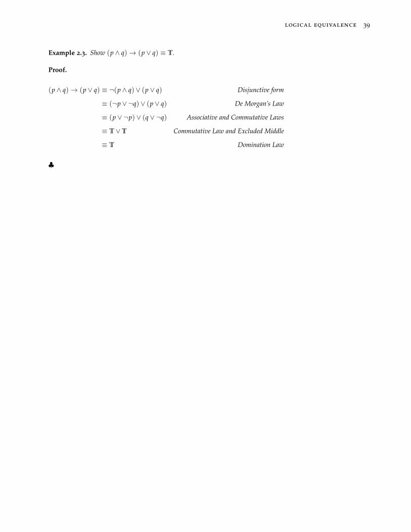
Example 2.3. Show (p ∧ q)→ (p ∨ q) ≡ T.
Proof.
(p ∧ q)→ (p ∨ q) ≡ ¬(p ∧ q) ∨ (p ∨ q) Disjunctive form
≡ (¬p ∨ ¬q) ∨ (p ∨ q) De Morgan’s Law
≡ (p ∨ ¬p) ∨ (q ∨ ¬q) Associative and Commutative Laws
≡ T∨T Commutative Law and Excluded Middle
≡ T Domination Law
♣
40 math208: discrete mathematics
2.7 Exercises
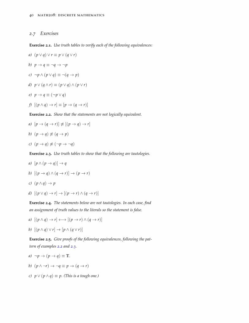
Exercise 2.1. Use truth tables to verify each of the following equivalences:
a) (p ∨ q) ∨ r ≡ p ∨ (q ∨ r)
b) p→ q ≡ ¬q→ ¬p
c) ¬p ∧ (p ∨ q) ≡ ¬(q→ p)
d) p ∨ (q ∧ r) ≡ (p ∨ q) ∧ (p ∨ r)
e) p→ q ≡ (¬p ∨ q)
f) [(p ∧ q)→ r] ≡ [p→ (q→ r)]
Exercise 2.2. Show that the statements are not logically equivalent.
a) [p→ (q→ r)] 6≡ [(p→ q)→ r]
b) (p→ q) 6≡ (q→ p)
c) (p→ q) 6≡ (¬p→ ¬q)
Exercise 2.3. Use truth tables to show that the following are tautologies.
a) [p ∧ (p→ q)]→ q
b) [(p→ q) ∧ (q→ r)]→ (p→ r)
c) (p ∧ q)→ p
d) [(p ∨ q)→ r]→ [(p→ r) ∧ (q→ r)]
Exercise 2.4. The statements below are not tautologies. In each case, find
an assignment of truth values to the literals so the statement is false.
a) [(p ∧ q)→ r]←→ [(p→ r) ∧ (q→ r)]
b) [(p ∧ q) ∨ r]→ [p ∧ (q ∨ r)]
Exercise 2.5. Give proofs of the following equivalences, following the pat-
tern of examples 2.2 and 2.3.
a) ¬p→ (p→ q) ≡ T.
b) (p ∧ ¬r)→ ¬q ≡ p→ (q→ r)
c) p ∨ (p ∧ q) ≡ p. (This is a tough one.)
3
Predicates and Quantifiers
The sentence x2 − 2 = 0 is not a proposition. It cannot be as-
signed a truth value unless some more information is supplied about
the variable x. Such a statement is called a predicate or a proposi-
tional function.
3.1 Predicates
Instead of using a single letter to denote a predicate, a symbol such
as S(x) will be used to indicate the dependence of the sentence on a
variable. Here are two more examples of predicates.
(1) A(c) : Al drives a c, and
(2) B(x, y) : x is the brother of y. The second example is an instance of a
two-place predicate.
With a given predicate, there is an associated set of objects which
can be used in place of the variables. For example, in the predicate
S(x) : x2 − 2 = 0, it is understood that the x can be replaced
by a number. Replacing x by, say, the word blue does not yield a
meaningful sentence. For the predicate A(c) above, c can be replaced
by, say, makes of cars (or maybe types of nails!). For B(x, y), the x Usually the domain of discourse is
left for the reader to guess, but if the
domain of discourse is something other
than an obvious choice, the writer will
mention the domain to be used.
can be replaced by any human male, and the y by any human. The
collection of possible replacements for a variable in a predicate is
called the domain of discourse for that variable.
42 math208: discrete mathematics
3.2 Instantiation and Quantification
A predicate is not a proposition, but it can be converted into a propo-
sition. There are three ways to modify a predicate to change it into a
proposition. Let’s use S(x) : x2 − 2 = 0 as an example.
The first way to change S(x) to make it into a proposition is to
assign a specific value from the variable’s domain of discourse to
the variable. For example, setting x = 3, gives the (false) proposi-
tion S(3) : 32 − 2 = 0. On the other hand, setting x =√
2 gives
the (true) proposition S(√
2) : (√
2)2 − 2 = 0. The process of set-
ting a variable equal to a specific object in its domain of discourse is
called instantiation. Looking at the two-place predicate B(x, y) : x
is the brother of y, we can instantiate both variables to get the (true)
proposition B(Donny, Marie) : Donny is the brother of Marie. Notice
that the sentence B(Donny, y) : Donny is the brother of y has not been
converted into a proposition since it cannot be assigned a truth value
without some information about y. But it has been converted from a
two-place predicate to a one-place predicate.
A second way to convert a predicate to a proposition is to precede
the predicate with the phrase There is an x such that. For example,
There is an x such that S(x) would become There is an x such that
x2 − 2 = 0. This proposition is true if there is at least one choice
of x in its domain of discourse for which the predicate becomes a
true statement. The phrase There is an x such that is denoted in sym-
bols by ∃x, so the proposition above would be written as ∃x S(x)
or ∃x (x2 − 2 = 0). When trying to determine the truth value of
the proposition ∃x P(x), it is important to keep the domain of dis-
course for the variable in mind. For example, if the domain for x in
∃x (x2 − 2 = 0) is all integers, the proposition is false. But if its
domain is all real numbers, the proposition is true. The phrase There
is an x such that (or, in symbols, ∃x) is called existential quantifica-
tion1. 1 In English it can also be read as Thereexists x or For some x.
The third and final way to convert a predicate into a proposition is
by universal quantification2 . The universal quantification of a pred- 2 The phrase For all x is also rendered inEnglish as For each x or For every x.
icate, P(x), is obtained by preceding the predicate with the phrase
predicates and quantifiers 43
For all x, producing the proposition For all x, P(x), or, in symbols,
∀x P(x). This proposition is true provided the predicate becomes
a true proposition for every object in the variable’s domain of dis-
course. Again, it is important to know the domain of discourse for
the variable since the domain will have an effect on the truth value of
the quantified proposition in general.
For multi-placed predicates, these three conversions can be mixed
and matched. For example, using the obvious domains for the pred-
icate B(x, y) : x is the brother of y here are some conversions into
propositions:
(1) B(Donny, Marie) has both variables instantiated. The proposition
is true.
(2) ∃y B(Donny, y) is also a true proposition. It says Donny is some-
body’s brother. The first variable was instantiated, the second was
existentially quantified.
(3) ∀y B(Donny, y) says everyone has Donny for a brother, and that is
false.
(4) ∀x ∃y B(x, y) says every male is somebody’s brother, and that is
false.
(5) ∃y ∀x B(x, y) says there is a person for whom every male is a
brother, and that is false.
(6) ∀x B(x, x) says every male is his own brother, and that is false.
3.3 Translating to symbolic form
Translation between ordinary language and symbolic language can
get a little tricky when quantified statements are involved. Here are a
few more examples.
Example 3.1. Let P(x) be the predicate x owns a Porsche, and let S(x) be
the predicate x speeds. The domain of discourse for the variable in each
predicate will be the collection of all drivers. The proposition ∃xP(x)
says Someone owns a Porsche. It could also be translated as There is
a person x such that x owns a Porsche, but that sounds too stilted for
44 math208: discrete mathematics
ordinary conversation. A smooth translation is better. The proposition
∀x(P(x)→ S(x)) says All Porsche owners speed.
Translating in the other direction, the proposition No speeder owns a
Porsche could be expressed as ∀x(S(x)→ ¬P(x)).
Example 3.2. Here’s a more complicated example: translate the proposition
Al knows only Bill into symbolic form. Let’s use K(x, y) for the predicate
x knows y. The translation would be K(Al, Bill) ∧ ∀x (K(Al, x) → (x =
Bill)).
Example 3.3. For one last example, let’s translate The sum of two even
integers is even into symbolic form. Let E(x) be the predicate x is even.
As with many statements in ordinary language, the proposition is phrased
in a shorthand code that the reader is expected to unravel. As given, the
statement doesn’t seem to have any quantifiers, but they are implied. Before
converting it to symbolic form, it might help to expand it to its more long
winded version: For every choice of two integers, if they are both even,
then their sum is even. Expressed this way, the translation to symbolic
form is duck soup: ∀x ∀y ((E(x) ∧ E(y))→ E(x + y)).
3.4 Quantification and basic laws of logic
Notice that if the domain of discourse consists of finitely many en-
tries a1, ..., an, then ∀x p(x) ≡ p(a1) ∧ p(a2) ∧ ... ∧ p(an). So the
quantifier ∀ can be expressed in terms of the logical connective
∧. The existential quantifier and ∨ are similarly linked: ∃x p(x) ≡p(a1) ∨ p(a2) ∨ ...∨ p(an).
From the associative and commutative laws of logic we see that we
can rearrange any system of propositions which are linked only by
∧’s or linked only by ∨’s.3 Consequently any more generally quan- 3 For instance, consider examples 3.1 –3.3 with finite domains of discourse.
tified proposition of the form ∀x∀y p(x, y) is logically equivalent to
∀y∀x p(x, y). Similarly for statements which contain only existential
quantifiers. But the distributive laws come into play when ∧’s and
∨’s are mixed. So care must be taken with predicates which contain
both existential and universal quantifiers, as the following example
shows.
predicates and quantifiers 45
Example 3.4. Let p(x, y) : x + y = 0 and let the domain of discourse be all
real numbers for both x and y. The proposition ∀y ∃x p(x, y) is true, since,
for any given y, by setting (instantiating) x = −y we convert x + y = 0 to
the true statement (−y) + y = 04. However the proposition ∃x ∀y p(x, y) 4 (∀y ∈ R)[(−y) + y = 0] is a tautology.
is false. If we set (instantiate) y = 1, then x + y = 0 implies that x = −1.
When we set y = 0, we get x = 0. Since 0 6= −1 there is no x which will
work for all y, since it would have to work for the specific values of y = 0
and y = 1.
3.5 Negating quantified statements
To form the negation of quantified statements, we apply De Mor-
gan’s laws. This can be seen in case of a finite domain of discourse as
follows:
¬(∀x p(x)) ≡ ¬(p(a1) ∧ p(a2) ∧ ...∧ p(an))
≡ ¬p(a1) ∨ ¬p(a2) ∨ · · · ∨ ¬p(an)
≡ ∃x¬p(x)
In the same way, we have ¬(∃x p(x)) ≡ (∀x¬p(x)). 5 5 Use De Morgan’s laws to find a similarexpression for ¬(∀xp(x)).
46 math208: discrete mathematics
3.6 Exercises
Exercise 3.1. Let p(x) : 2x ≥ 4. Determine the truth values of the
following propositions.
a) p(2)
b) p(−3)
c) ∀x ((x ≤ 10)→ p(x))
d) ∃x¬p(x)
Exercise 3.2. Let p(x, y) be x has read y, where the domain of discourse for
x is all students in this class, and the domain of discourse for y is all novels.
Express the following propositions in English.
a) ∀x p(x, War and Peace)
b) ∃x¬p(x, The Great Gatsby)
c) ∃x ∀y p(x, y)
d) ∀y ∃x p(x, y)
Exercise 3.3. Let F(x, y) be the statement x can fool y, where the domain of
discourse for both x and y is all people. Use quantifiers to express each of the
following statements.
a) I can fool everyone.
b) George can’t fool anybody.
c) No one can fool himself.
d) There is someone who can fool everybody.
e) There is someone everyone can fool.
f) Ralph can fool two different people.
Exercise 3.4. Negate each of the statements from exercise 3.2 in English.
Exercise 3.5. Negate each statement from exercise 3.3 in logical symbols.
Of course, the easy answer would be to simply put ¬ in front of each state-
ment. But use the principle given at the end of this chapter to move the
negation across the quantifiers.
predicates and quantifiers 47
Exercise 3.6. Express symbolically: The product of an even integer and an
odd integer is even.
Exercise 3.7. Express in words the meaning of
∃xP(x) ∧ ∀x∀y ((P(x) ∧ P(y))→ (x = y)).

4
Rules of Inference
The heart of mathematics is proof. In this chapter, we give a
careful description of what exactly constitutes a proof in the realm
of propositional logic. Throughout the course various methods of
proof will be demonstrated, including the particularly important
style of proof called induction. It’s important to keep in mind that all
proofs, no matter what the subject matter might be, are based on the
notion of a valid argument as described in this chapter, so the ideas
presented here are fundamental to all of mathematics.
Imagine trying carefully to define what a proof is, and it quickly
becomes clear just how difficult a task that is. So it shouldn’t come as
a surprise that the description takes on a somewhat technical looking
aspect. But don’t let all the symbols and abstract-looking notation
be misleading. All these rules really boil down to plain old common
sense when looked at correctly.
The usual form of a theorem in mathematics is: If a is true and b is
true and c is true, etc., then s is true. The a, b, c, · · · are called the hy-
potheses, and the statement s is called the conclusion. For example,
a mathematical theorem might be: if m is an even integer and n is an
odd integer, then mn is an even integer. Here the hypotheses are m is
an even integer and n is and odd integer, and the conclusion is mn is an
even integer.
50 math208: discrete mathematics
4.1 Valid propositional arguments
In this section we are going to be concerned with proofs from the
realm of propositional logic rather than the sort of theorem from
mathematics mentioned above. We will be interested in arguments in
which the form of the argument is the item of interest rather than the
content of the statements in the argument.
For example, consider the simple argument: (1) My car is either
red or blue and (2) My car is not red, and so (3) My car is blue. Here
the hypotheses are (1) and (2), and the conclusion is (3). It should be
clear that this is a valid argument. That means that if you agree that
(1) and (2) are true, then you must accept that (3) is true as well.
Definition 4.1. An argument is called valid provided that if you
agree that all the hypotheses are true, then you must accept the truth
of the conclusion.
Now the content of that argument (in other words, the stuff about
my and cars and colors) really have nothing to do with the validity
of the argument. It is the form of the argument that makes it valid.
The form of this argument is (1) p ∨ q and (2) ¬p, therefore (3) q. Any
argument that has this form is valid, whether it talks about cars and
colors or any other notions. For example, here is another argument of
the very same form: (1) I either read the book or just looked at the pictures
and (2) I didn’t read the book, therefore (3) I just looked at the pictures.
Some arguments involve quantifiers. For instance, consider the
classic example of a logical argument: (1) All men are mortal and (2)
Socrates is a man, and so (3) Socrates is mortal. Here the hypotheses
are the statements (1) and (2), and the conclusion is statement (3).
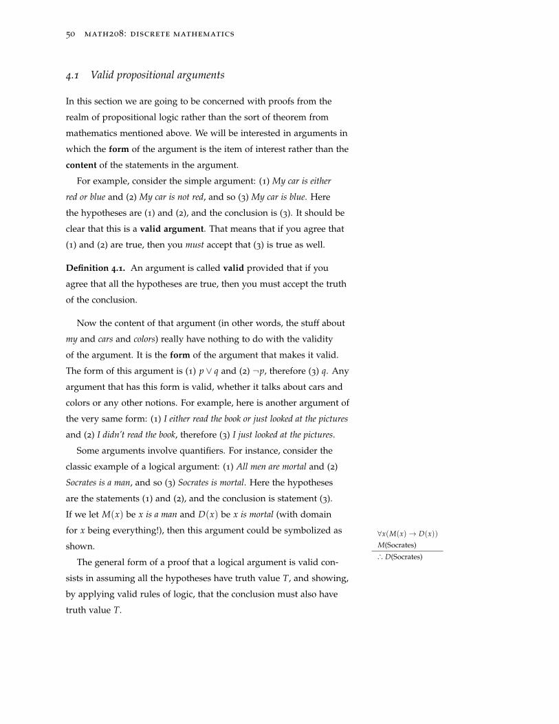
If we let M(x) be x is a man and D(x) be x is mortal (with domain
for x being everything!), then this argument could be symbolized as
shown.∀x(M(x)→ D(x))
M(Socrates)
... D(Socrates)The general form of a proof that a logical argument is valid con-
sists in assuming all the hypotheses have truth value T, and showing,
by applying valid rules of logic, that the conclusion must also have
truth value T.
rules of inference 51
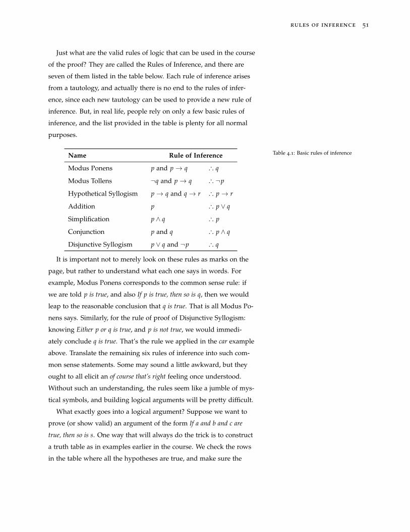
Just what are the valid rules of logic that can be used in the course
of the proof? They are called the Rules of Inference, and there are
seven of them listed in the table below. Each rule of inference arises
from a tautology, and actually there is no end to the rules of infer-
ence, since each new tautology can be used to provide a new rule of
inference. But, in real life, people rely on only a few basic rules of
inference, and the list provided in the table is plenty for all normal
purposes.
Name Rule of Inference
Modus Ponens p and p→ q ... q
Modus Tollens ¬q and p→ q ... ¬p
Hypothetical Syllogism p→ q and q→ r ... p→ r
Addition p ... p ∨ q
Simplification p ∧ q ... p
Conjunction p and q ... p ∧ q
Disjunctive Syllogism p ∨ q and ¬p ... q
Table 4.1: Basic rules of inference
It is important not to merely look on these rules as marks on the
page, but rather to understand what each one says in words. For
example, Modus Ponens corresponds to the common sense rule: if
we are told p is true, and also If p is true, then so is q, then we would
leap to the reasonable conclusion that q is true. That is all Modus Po-
nens says. Similarly, for the rule of proof of Disjunctive Syllogism:
knowing Either p or q is true, and p is not true, we would immedi-
ately conclude q is true. That’s the rule we applied in the car example
above. Translate the remaining six rules of inference into such com-
mon sense statements. Some may sound a little awkward, but they
ought to all elicit an of course that’s right feeling once understood.
Without such an understanding, the rules seem like a jumble of mys-
tical symbols, and building logical arguments will be pretty difficult.
What exactly goes into a logical argument? Suppose we want to
prove (or show valid) an argument of the form If a and b and c are
true, then so is s. One way that will always do the trick is to construct
a truth table as in examples earlier in the course. We check the rows
in the table where all the hypotheses are true, and make sure the
52 math208: discrete mathematics
conclusion is also true in those rows. That would complete the proof.
In fact that is exactly the method used to justify the seven rules of
inference given in the table. But building truth tables is certainly
tedious business, and it certainly doesn’t seem too much like the way
we learned to do proofs in geometry, for example. An alternative is
the construction of a logical argument which begins by assuming the
hypotheses are all true and applies the basic rules of inferences from
the table until the desired conclusion is shown to be true.
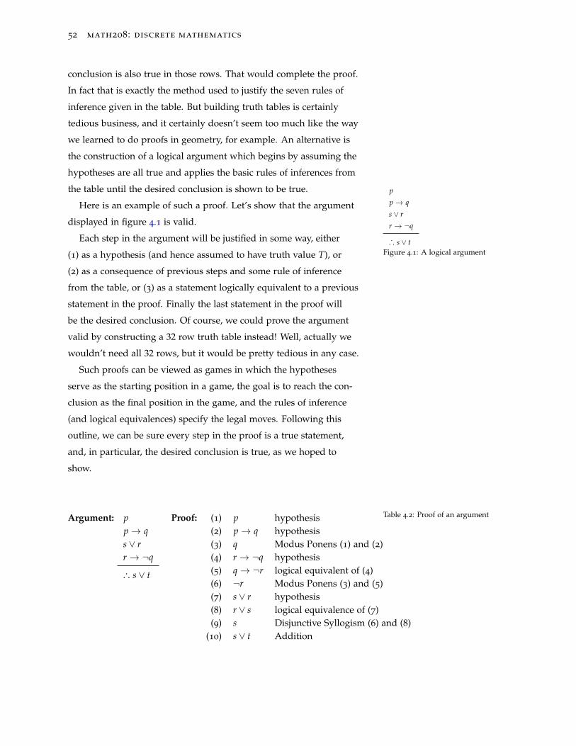
Here is an example of such a proof. Let’s show that the argument
displayed in figure 4.1 is valid.
p
p→ q
s ∨ r
r → ¬q
... s ∨ tFigure 4.1: A logical argument
Each step in the argument will be justified in some way, either
(1) as a hypothesis (and hence assumed to have truth value T), or
(2) as a consequence of previous steps and some rule of inference
from the table, or (3) as a statement logically equivalent to a previous
statement in the proof. Finally the last statement in the proof will
be the desired conclusion. Of course, we could prove the argument
valid by constructing a 32 row truth table instead! Well, actually we
wouldn’t need all 32 rows, but it would be pretty tedious in any case.
Such proofs can be viewed as games in which the hypotheses
serve as the starting position in a game, the goal is to reach the con-
clusion as the final position in the game, and the rules of inference
(and logical equivalences) specify the legal moves. Following this
outline, we can be sure every step in the proof is a true statement,
and, in particular, the desired conclusion is true, as we hoped to
show.
Argument: pp→ qs ∨ rr → ¬q
... s ∨ t
Proof: (1) p hypothesis(2) p→ q hypothesis(3) q Modus Ponens (1) and (2)(4) r → ¬q hypothesis(5) q→ ¬r logical equivalent of (4)(6) ¬r Modus Ponens (3) and (5)(7) s ∨ r hypothesis(8) r ∨ s logical equivalence of (7)(9) s Disjunctive Syllogism (6) and (8)
(10) s ∨ t Addition
Table 4.2: Proof of an argument
rules of inference 53
One step more complicated than the last example are arguments
that are presented in words rather than symbols. In such a case, it is
necessary to first convert from a verbal argument to a symbolic argu-
ment, and then check the argument to see if it is valid. For example,
consider the argument: Tom is a cat. If Tom is a cat, then Tom likes fish.
Either Tweety is a bird or Fido is a dog. If Fido is a dog, then Tom does not
like fish. So, either Tweety is a bird or I’m a monkey’s uncle. Just reading
this argument, it is difficult to decide if it is valid or not. It’s just a
little too confusing to process. But it is valid, and in fact it is the very
same argument as given above. Let p be Tom is a cat, let q be Tom likes
fish, let s be Tweety is a bird, let r be Fido is a dog, and let t be I’m a
monkey’s uncle. Expressing the statements in the argument in terms of
p, q, r, s, t produces exactly the symbolic argument proved above.
4.2 Fallacies
Some logical arguments have a convincing ring to them but are nev-
ertheless invalid. The classic example is an argument of the form If
it is snowing, then it is winter. It is winter. So it must be snowing. A mo-
ment’s thought is all that is needed to be convinced the conclusion
does not follow from the two hypotheses. Indeed, there are many
winter days when it does not snow. The error being made is called
the fallacy of affirming the conclusion. In symbols, the argument is
claiming that [(p → q) ∧ q] → p is a tautology, but in fact, checking a
truth table shows that it is not a tautology. Fallacies arise when state-
ments that are not tautologies are treated as if they were tautologies.
4.3 Arguments with quantifiers
Logical arguments involving propositions using quantifiers require a
few more rules of inference. As before, these rules really amount to
no more than a formal way to express common sense. For instance, if
the proposition ∀ x P(x) is true, then certainly for every object c in the
universe of discourse, P(c) is true. After all, if the statement P(x) is
true for every possible choice of x, then, in particular, it is true when
x = c. The other three rules of inference for quantified statements are
54 math208: discrete mathematics
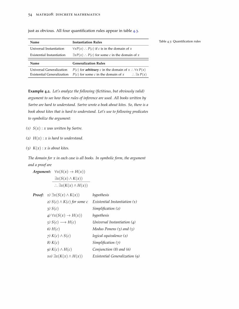
just as obvious. All four quantification rules appear in table 4.3.
Name Instantiation Rules
Universal Instantiation ∀xP(x) ... P(c) if c is in the domain of x
Existential Instantiation ∃xP(x) ... P(c) for some c in the domain of x
Name Generalization Rules
Universal Generalization P(c) for arbitrary c in the domain of x ... ∀x P(x)Existential Generalization P(c) for some c in the domain of x ... ∃x P(x)
Table 4.3: Quantification rules
Example 4.2. Let’s analyze the following (fictitious, but obviously valid)
argument to see how these rules of inference are used. All books written by
Sartre are hard to understand. Sartre wrote a book about kites. So, there is a
book about kites that is hard to understand. Let’s use to following predicates
to symbolize the argument:
(1) S(x) : x was written by Sartre.
(2) H(x) : x is hard to understand.
(3) K(x) : x is about kites.
The domain for x in each case is all books. In symbolic form, the argument
and a proof are
Argument: ∀x(S(x)→ H(x))
∃x(S(x) ∧ K(x))
... ∃x(K(x) ∧ H(x))
Proof: 1) ∃x(S(x) ∧ K(x)) hypothesis
2) S(c) ∧ K(c) for some c Existential Instantiation (1)
3) S(c) Simplification (2)
4) ∀x(S(x)→ H(x)) hypothesis
5) S(c) −→ H(c) Universal Instantiation (4)
6) H(c) Modus Ponens (3) and (5)
7) K(c) ∧ S(c) logical equivalence (2)
8) K(c) Simplification (7)
9) K(c) ∧ H(c) Conjunction (8) and (6)
10) ∃x(K(x) ∧ H(x)) Existential Generalization (9)
rules of inference 55
4.4 Exercises
Exercise 4.1. Show p ∨ q and ¬p ∨ r, ... q ∨ r is a valid rule of inference.
It is called Resolution.
Exercise 4.2. Show that p −→ q and ¬p, ... ¬q is not a valid rule of
inference. It is called the Fallacy of denying the hypothesis.
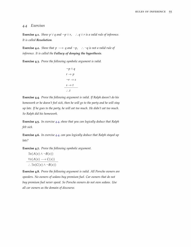
Exercise 4.3. Prove the following symbolic argument is valid.
¬p ∧ q
r → p
¬r → s
s→ t
... t
Exercise 4.4. Prove the following argument is valid. If Ralph doesn’t do his
homework or he doesn’t feel sick, then he will go to the party and he will stay
up late. If he goes to the party, he will eat too much. He didn’t eat too much.
So Ralph did his homework.
Exercise 4.5. In exercise 4.4, show that you can logically deduce that Ralph
felt sick.
Exercise 4.6. In exercise 4.4, can you logically deduce that Ralph stayed up
late?
Exercise 4.7. Prove the following symbolic argument.
∃x(A(x) ∧ ¬B(x))
∀x(A(x) −→ C(x))
... ∃x(C(x) ∧ ¬B(x))
Exercise 4.8. Prove the following argument is valid. All Porsche owners are
speeders. No owners of sedans buy premium fuel. Car owners that do not
buy premium fuel never speed. So Porsche owners do not own sedans. Use
all car owners as the domain of discourse.

5
Sets: Basic Definitions
A set is a collection of objects. Often, but not always, sets are
denoted by capital letters such as A, B, · · · and the objects that make
up a set, called its elements, are denoted by lowercase letters. Write
x ∈ A to mean that the object x is an element of A. If the object x is
not an element of A, write x 6∈ A.
Two sets A and B are equal, written A = B provided A and B
comprise exactly the same elements. Another way to say the same
thing: A = B provided ∀x (x ∈ A←→ x ∈ B).
5.1 Specifying sets
There are a number of ways to specify a given set. We consider two
of them.
5.1.1 Roster method
One way to describe a set is to list its elements. This is called the
roster method. Braces are used to signify when the list begins and
where it ends, and commas are used to separate elements. For in-
stance, A = {1, 2, 3, 4, 5} is the set of positive whole numbers between
1 and 5 inclusive. It is important to note that the order in which el-
ements are listed is immaterial. For example, {1, 2} = {2, 1} since
x ∈ {1, 2} and x ∈ {2, 1} are both true for x = 1 and x = 2 and false
for all other choices of x. Thus x ∈ {1, 2} and x ∈ {2, 1} always have
the same truth value, and that means ∀x (x ∈ {1, 2} ←→ x ∈ {2, 1})
58 math208: discrete mathematics
is true. According to the definition of equality given above, it follows
that {1, 2} = {2, 1}. The same sort of reasoning shows that repe-
titions in the list of elements of a set can be ignored. For example
{1, 2, 3, 2, 4, 1, 2, 3, 2} = {1, 2, 3, 4}. There is no point in listing an
element of a set more than once.
The roster method has certain drawbacks. For example we prob-
ably don’t want to list all of the elements in the set of positive in-
tegers between 1 and 99 inclusive. One option is to use an ellipsis.
The idea is that we list elements until a pattern is established, and The use of an ellipsis has one pitfall.
It is hoped that whoever is reading
the list will be able guess the proper
pattern and apply it to fill in the gap.
then replace the missing elements with . . . (which is the ellipsis). So
{1, 2, 3, 4, . . . , 99} would describe our set.
5.1.2 Set-builder notation
Another method to specify a set is via the use of set-builder nota-
tion. A set can be described in set-builder notation as A = {x|p(x)}.Here we read A is the set of all objects x for which the predicate p(x)
is true. So {1, 2, 3, 4, . . . , 99} becomes {x|x is a whole number and
1 ≤ x ≤ 99}.
5.2 Special standard sets
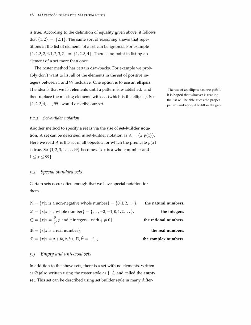
Certain sets occur often enough that we have special notation for
them.
N = {x|x is a non-negative whole number} = {0, 1, 2, . . . }, the natural numbers.
Z = {x|x is a whole number} = {. . . ,−2,−1, 0, 1, 2, . . . }, the integers.
Q = {x|x =pq
, p and q integers with q 6= 0}, the rational numbers.
R = {x|x is a real number}, the real numbers.
C = {x|x = a + ib, a, b ∈ R, i2 = −1}, the complex numbers.
5.3 Empty and universal sets
In addition to the above sets, there is a set with no elements, written
as ∅ (also written using the roster style as { }), and called the empty
set. This set can be described using set builder style in many differ-
sets: basic definitions 59
ent ways. For example, {x ∈ R|x2 = −2} = ∅. In fact, if P(x) is any
predicate which is always false, then {x | P(x)} = ∅. There are two
easy slips to make involving the empty set. First, don’t write ∅ = 0
(the idea being that both ∅ and 0 represent nothing1). That is not cor- 1 One is empty the other is something,namely zero.
rect since ∅ is a set, and 0 is a number, and it’s not fair to compare
two different types of objects. The other error is thinking ∅ = {∅}.This cannot be correct since the right-hand set has an element, but
the left-hand set does not.
At the other extreme from the empty set is the universal set, de-
noted U . The universal set consists of all objects under consideration
in any particular discussion. For example, if the topic du jour is basic
arithmetic then the universal set would be the set of all integers. Usu-
ally the universal set is left for the reader to guess. If the choice of the
universal set is not an obvious one, it will be pointed out explicitly.
5.4 Subset and equality relations
The set A is a subset of the set B, written as A ⊆ B, in case ∀x(x ∈A −→ x ∈ B) is true. In plain English, A ⊆ B if every element of
A also is an element of B. For example, {1, 2, 3} ⊆ {1, 2, 3, 4, 5}. On
the other hand, {0, 1, 2, 3} 6⊆ {1, 2, 3, 4, 5} since 0 is an element of the
left-hand set but not of the right-hand set. The meaning of A 6⊆ B can
be expressed in symbols using De Morgan’s law:
A 6⊆ B←→ ¬(∀x(x ∈ A→ x ∈ B))
≡ ∃x¬(x ∈ A→ x ∈ B)
≡ ∃x¬(¬(x ∈ A) ∨ x ∈ B)
≡ ∃x(x ∈ A ∧ x 6∈ B)
and that last line says A 6⊆ B provided there is at least one element of
A that is not an element of B.
The empty set is a subset of every set. To check that, suppose A is
any set, and let’s check to make sure ∀x(x ∈ ∅ −→ x ∈ A) is true.
But it is since for any x, the hypothesis of x ∈ ∅ −→ x ∈ A is F, and
so the implication is T. So ∅ ⊆ A. Another way to same the same
60 math208: discrete mathematics
thing is to notice that to claim ∅ 6⊆ A is the same as claiming there
is at least one element of ∅ that is not an element of A, but that is
ridiculous, since ∅ has no elements at all.
To say that A = B is the same as saying every element of A is also
an element of B and every element of B is also an element of A. In
other words, A = B ←→ (A ⊆ B ∧ B ⊆ A), and this indicates the
method by which the common task of showing two sets are equal is
carried out: to show two sets are equal, show that each is a subset of
the other.
If A ⊆ B, and A 6= B, A is a proper subset of B, denoted by
A ⊂ B, or A⊂6= B. In words, A ⊂ B means every element of A is also
an element of B and there is at least one element of B that is not an
element of A. For example {1, 2} ⊂ {1, 2, 3, 4, 5}, and ∅ ⊂ {1}.
5.5 Cardinality
A set is finite if the number of distinct elements in the set is a non-
negative integer. In this case we call the number of distinct ele-
ments in the set its cardinality and denote this natural number by
|A|. For example, |{1, 3, 5}| = 3 and |∅| = 0, |{∅}| = 1, and
|{∅, {a, b, c}, {X, Y}}| = 3. A set, such as Z, which is not finite, is
infinite.
5.6 Power set
Given a set A the power set of A, denoted P(A), is the set of all sub-
sets of A. For example if A = {1, 2}, then P(A) = {∅, {1}, {2}, {1, 2}}.For a more confusing example, the power set of {∅, {∅}}2 is 2 Try finding the power set of the empty
set: P(∅).
P ({∅, {∅}}) = {∅, {∅}, {{∅}}, {∅, {∅}}}.
It is not hard to see that if |A| = n, then |P(A)| = 2n.
sets: basic definitions 61
5.7 Exercises
Exercise 5.1. List the members of the following sets.
a) {x ∈ Z|3 ≤ x3 < 100}
b) {x ∈ R|2x2 = 50}
c) {x ∈N|7 > x ≥ 4}
Exercise 5.2. Use set-builder notation to give a description of each set.
a) {−5, 0, 5, 10, 15}
b) {0, 1, 2, 3, 4}
c) The interval of real numbers: [π, 4)
Exercise 5.3. Determine the cardinality of the sets in exercises 1 and 2.
Exercise 5.4. Is the proposition Every element of the empty set has three
toes true or false? Explain your answer!
Exercise 5.5. Determine the power set of {1, ∅, {1}}.

6
Set Operations
There are several ways of combining sets to produce new sets.
6.1 Intersection
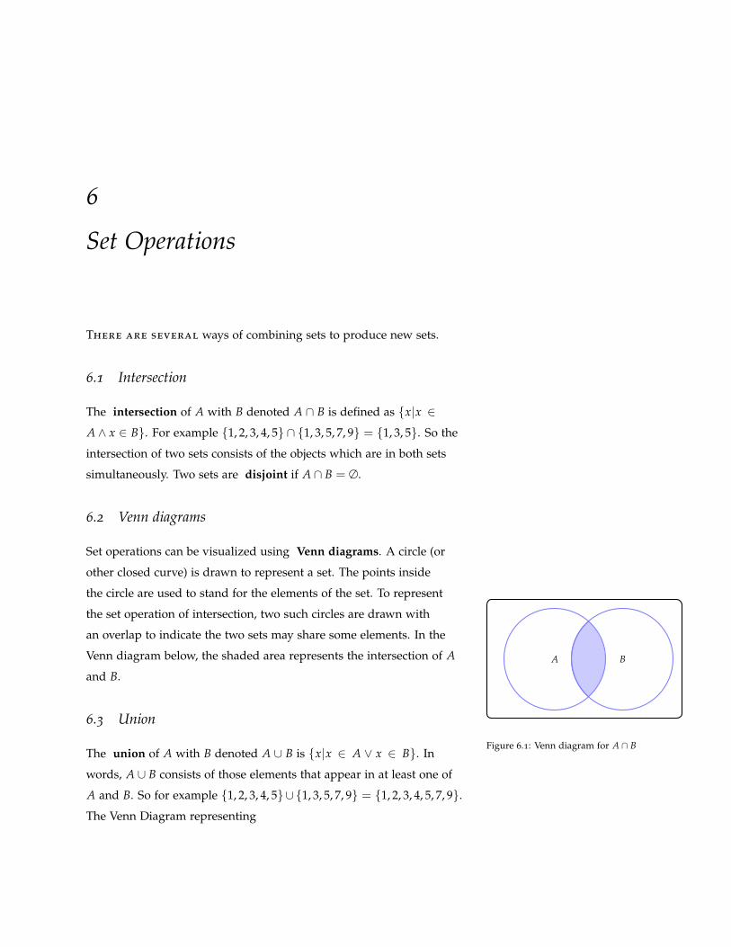
The intersection of A with B denoted A ∩ B is defined as {x|x ∈A ∧ x ∈ B}. For example {1, 2, 3, 4, 5} ∩ {1, 3, 5, 7, 9} = {1, 3, 5}. So the
intersection of two sets consists of the objects which are in both sets
simultaneously. Two sets are disjoint if A ∩ B = ∅.
6.2 Venn diagrams
Set operations can be visualized using Venn diagrams. A circle (or
other closed curve) is drawn to represent a set. The points inside
the circle are used to stand for the elements of the set. To represent
the set operation of intersection, two such circles are drawn with
an overlap to indicate the two sets may share some elements. In the
Venn diagram below, the shaded area represents the intersection of A
and B.A B
Figure 6.1: Venn diagram for A ∩ B
6.3 Union
The union of A with B denoted A ∪ B is {x|x ∈ A ∨ x ∈ B}. In
words, A ∪ B consists of those elements that appear in at least one of
A and B. So for example {1, 2, 3, 4, 5}∪{1, 3, 5, 7, 9} = {1, 2, 3, 4, 5, 7, 9}.The Venn Diagram representing
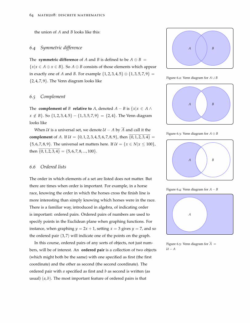
64 math208: discrete mathematics
the union of A and B looks like this:
A B
Figure 6.2: Venn diagram for A ∪ B
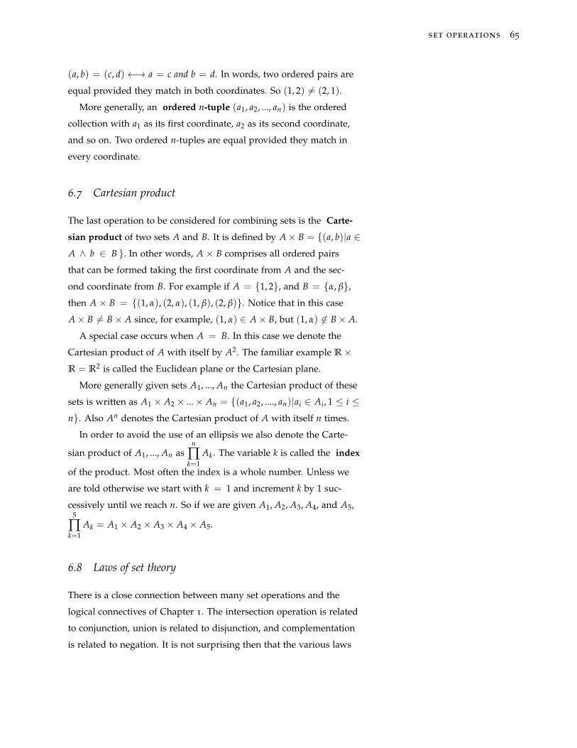
6.4 Symmetric difference
The symmetric difference of A and B is defined to be A ⊕ B =
{x|x ∈ A⊕ x ∈ B}. So A⊕ B consists of those elements which appear
in exactly one of A and B. For example {1, 2, 3, 4, 5} ⊕ {1, 3, 5, 7, 9} ={2, 4, 7, 9}. The Venn diagram looks like
A B
Figure 6.3: Venn diagram for A⊕ B
6.5 Complement
The complement of B relative to A, denoted A− B is {x|x ∈ A ∧x 6∈ B}. So {1, 2, 3, 4, 5} − {1, 3, 5, 7, 9} = {2, 4}. The Venn diagram
looks like
A B
Figure 6.4: Venn diagram for A− B
When U is a universal set, we denote U − A by A and call it the
complement of A. If U = {0, 1, 2, 3, 4, 5, 6, 7, 8, 9}, then {0, 1, 2, 3, 4} ={5, 6, 7, 8, 9}. The universal set matters here. If U = {x ∈ N|x ≤ 100},then {0, 1, 2, 3, 4} = {5, 6, 7, 8, ..., 100}.
A
Figure 6.5: Venn diagram for A =
U − A
6.6 Ordered lists
The order in which elements of a set are listed does not matter. But
there are times when order is important. For example, in a horse
race, knowing the order in which the horses cross the finish line is
more interesting than simply knowing which horses were in the race.
There is a familiar way, introduced in algebra, of indicating order
is important: ordered pairs. Ordered pairs of numbers are used to
specify points in the Euclidean plane when graphing functions. For
instance, when graphing y = 2x + 1, setting x = 3 gives y = 7, and so
the ordered pair (3, 7) will indicate one of the points on the graph.
In this course, ordered pairs of any sorts of objects, not just num-
bers, will be of interest. An ordered pair is a collection of two objects
(which might both be the same) with one specified as first (the first
coordinate) and the other as second (the second coordinate). The
ordered pair with a specified as first and b as second is written (as
usual) (a, b). The most important feature of ordered pairs is that
set operations 65
(a, b) = (c, d)←→ a = c and b = d. In words, two ordered pairs are
equal provided they match in both coordinates. So (1, 2) 6= (2, 1).
More generally, an ordered n-tuple (a1, a2, ..., an) is the ordered
collection with a1 as its first coordinate, a2 as its second coordinate,
and so on. Two ordered n-tuples are equal provided they match in
every coordinate.
6.7 Cartesian product
The last operation to be considered for combining sets is the Carte-
sian product of two sets A and B. It is defined by A× B = {(a, b)|a ∈A ∧ b ∈ B }. In other words, A × B comprises all ordered pairs
that can be formed taking the first coordinate from A and the sec-
ond coordinate from B. For example if A = {1, 2}, and B = {α, β},then A × B = {(1, α), (2, α), (1, β), (2, β)}. Notice that in this case
A× B 6= B× A since, for example, (1, α) ∈ A× B, but (1, α) 6∈ B× A.
A special case occurs when A = B. In this case we denote the
Cartesian product of A with itself by A2. The familiar example R×R = R2 is called the Euclidean plane or the Cartesian plane.
More generally given sets A1, ..., An the Cartesian product of these
sets is written as A1 × A2 × ...× An = {(a1, a2, ...., an)|ai ∈ Ai, 1 ≤ i ≤n}. Also An denotes the Cartesian product of A with itself n times.
In order to avoid the use of an ellipsis we also denote the Carte-
sian product of A1, ..., An asn
∏k=1
Ak. The variable k is called the index
of the product. Most often the index is a whole number. Unless we
are told otherwise we start with k = 1 and increment k by 1 suc-
cessively until we reach n. So if we are given A1, A2, A3, A4, and A5,5
∏k=1
Ak = A1 × A2 × A3 × A4 × A5.
6.8 Laws of set theory
There is a close connection between many set operations and the
logical connectives of Chapter 1. The intersection operation is related
to conjunction, union is related to disjunction, and complementation
is related to negation. It is not surprising then that the various laws
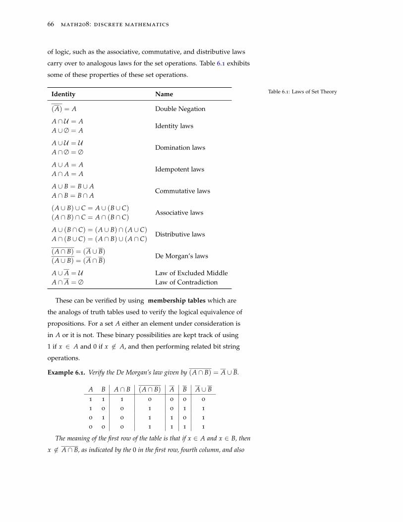
66 math208: discrete mathematics
of logic, such as the associative, commutative, and distributive laws
carry over to analogous laws for the set operations. Table 6.1 exhibits
some of these properties of these set operations.
Identity Name
(A) = A Double Negation
A ∩ U = AIdentity laws
A ∪∅ = A
A ∪ U = UDomination laws
A ∩∅ = ∅
A ∪ A = AIdempotent laws
A ∩ A = A
A ∪ B = B ∪ ACommutative laws
A ∩ B = B ∩ A
(A ∪ B) ∪ C = A ∪ (B ∪ C)Associative laws
(A ∩ B) ∩ C = A ∩ (B ∩ C)
A ∪ (B ∩ C) = (A ∪ B) ∩ (A ∪ C)Distributive laws
A ∩ (B ∪ C) = (A ∩ B) ∪ (A ∩ C)
(A ∩ B) = (A ∪ B)De Morgan’s laws
(A ∪ B) = (A ∩ B)
A ∪ A = U Law of Excluded MiddleA ∩ A = ∅ Law of Contradiction
Table 6.1: Laws of Set Theory
These can be verified by using membership tables which are
the analogs of truth tables used to verify the logical equivalence of
propositions. For a set A either an element under consideration is
in A or it is not. These binary possibilities are kept track of using
1 if x ∈ A and 0 if x 6∈ A, and then performing related bit string
operations.
Example 6.1. Verify the De Morgan’s law given by (A ∩ B) = A ∪ B.
A B A ∩ B (A ∩ B) A B A ∪ B1 1 1 0 0 0 0
1 0 0 1 0 1 1
0 1 0 1 1 0 1
0 0 0 1 1 1 1
The meaning of the first row of the table is that if x ∈ A and x ∈ B, then
x 6∈ A ∩ B, as indicated by the 0 in the first row, fourth column, and also
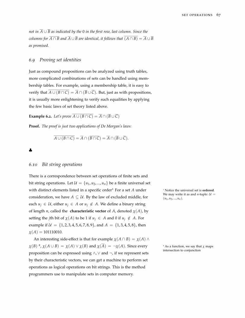
set operations 67
not in A ∪ B as indicated by the 0 in the first row, last column. Since the
columns for A ∩ B and A∪ B are identical, it follows that (A ∩ B) = A∪ B
as promised.
6.9 Proving set identities
Just as compound propositions can be analyzed using truth tables,
more complicated combinations of sets can be handled using mem-
bership tables. For example, using a membership table, it is easy to
verify that A ∪ (B ∩ C) = A ∩ (B ∪ C). But, just as with propositions,
it is usually more enlightening to verify such equalities by applying
the few basic laws of set theory listed above.
Example 6.2. Let’s prove A ∪ (B ∩ C) = A ∩ (B ∪ C)
Proof. The proof is just two applications of De Morgan’s laws:
A ∪ (B ∩ C) = A ∩ (B ∩ C) = A ∩ (B ∪ C).
♣
6.10 Bit string operations
There is a correspondence between set operations of finite sets and
bit string operations. Let U = {u1, u2, ..., un} be a finite universal set
with distinct elements listed in a specific order1 For a set A under 1 Notice the universal set is ordered.We may write it as and n-tuple: U =(u1, u2, ..., un).consideration, we have A ⊆ U . By the law of excluded middle, for
each uj ∈ U , either uj ∈ A or uj 6∈ A. We define a binary string
of length n, called the characteristic vector of A, denoted χ(A), by
setting the jth bit of χ(A) to be 1 if uj ∈ A and 0 if uj 6∈ A. For
example if U = {1, 2, 3, 4, 5, 6, 7, 8, 9}, and A = {1, 3, 4, 5, 8}, then
χ(A) = 101110010.
An interesting side-effect is that for example χ(A ∩ B) = χ(A) ∧χ(B) 2, χ(A ∪ B) = χ(A) ∨ χ(B) and χ(A) = ¬χ(A). Since every 2 As a function, we say that χ maps
intersection to conjunctionproposition can be expressed using ∧,∨ and ¬, if we represent sets
by their characteristic vectors, we can get a machine to perform set
operations as logical operations on bit strings. This is the method
programmers use to manipulate sets in computer memory.
68 math208: discrete mathematics
6.11 Exercises
Exercise 6.1. Let A = {2, 3, 4, 5, 6, 7, 8} and B = {1, 2, 4, 6, 7, 8, 9}. Find
a) A ∩ B
b) A ∪ B
c) A− B
d) B− A
Exercise 6.2. Determine the sets A and B, if A− B = {1, 2, 7, 8}, B− A =
{3, 4, 10} and A ∩ B = {5, 6, 9}.
Exercise 6.3. Use membership tables to show that A ⊕ B = (A ∪ B) −(A ∩ B).
Exercise 6.4. Do exercise 3 using Venn diagrams.
Exercise 6.5. Verify A ∪ (A ∩ B) = A.
Exercise 6.6. Let A = {1, 2, 3, 4}, B = {a, b, c}, C = {α, β}, and
D = {7, 8, 9}. Write out the following Cartesian products.
(a) A× B (b) B× A (c) C× B× D
Exercise 6.7. What can you conclude about A and B if A× B = B× A.
Exercise 6.8. If U = {0, 1, 2, 3, 4, 5, 6, 7, 8, 9}, determine χ({1, 2, 4, 8}).
Exercise 6.9. Let A = {1, 2, 3} × {1, 2, 3, 4}. List the elements of the set
B = {(s, t) ∈ A | s < t }.
7
Styles of Proof
Earlier, we practiced proving the validity of logical arguments,
both with and without quantifiers. The technique introduced there
is one of the main tools for constructing proofs in a more general
setting. In this chapter, various common styles of proof in mathemat-
ics are described. Recognizing these styles of proof will make both
reading and constructing proofs a little less onerous. The example proofs in this chapter will
use some familiar facts about integers,
which we will prove in a later chapter.
7.1 Direct proof
As mentioned before, the typical form of the statement of a theorem
is: if a and b and c and · · · , then d. The propositions a,b,c, · · · are called
the hypotheses, and the proposition d is called the conclusion. The
goal of the proof is to show that (a ∧ b ∧ c ∧ · · · ) → d is a true propo-
sition. In the case of propositional logic, the only thing that matters is
the form of a logical argument, not the particular propositions that are
involved. That means the proof can always be given in the form of a
truth table. In areas outside of propositional logic that is no longer
possible. Now the content of the propositions must be considered.
In other words, what the words mean, and not merely how they are
strung together, becomes important.
Suppose we want to prove an implication Theorem: If p, then
q. In other words, we want to show p → q is true. There are two
possibilities: Either p is false, in which case p → q is automatically
true, or p is true. In this second case, we need to show that q is true
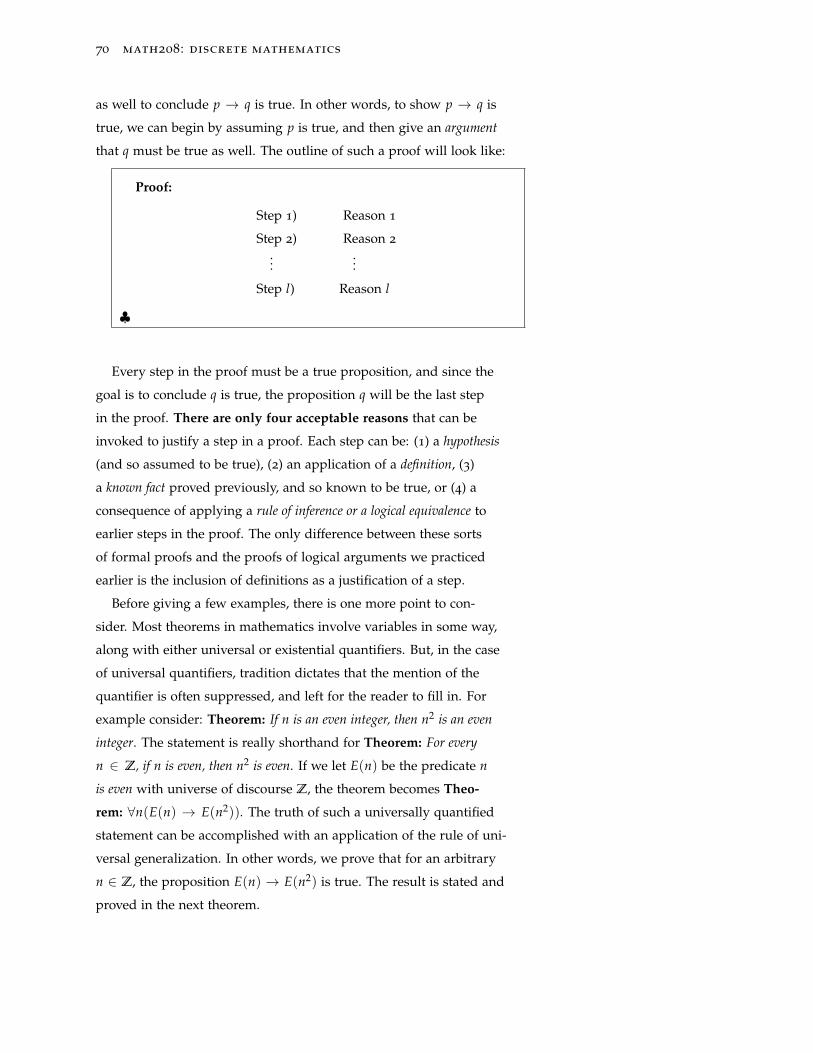
70 math208: discrete mathematics
as well to conclude p → q is true. In other words, to show p → q is
true, we can begin by assuming p is true, and then give an argument
that q must be true as well. The outline of such a proof will look like:
Proof:
Step 1) Reason 1
Step 2) Reason 2
......
Step l) Reason l
♣
Every step in the proof must be a true proposition, and since the
goal is to conclude q is true, the proposition q will be the last step
in the proof. There are only four acceptable reasons that can be
invoked to justify a step in a proof. Each step can be: (1) a hypothesis
(and so assumed to be true), (2) an application of a definition, (3)
a known fact proved previously, and so known to be true, or (4) a
consequence of applying a rule of inference or a logical equivalence to
earlier steps in the proof. The only difference between these sorts
of formal proofs and the proofs of logical arguments we practiced
earlier is the inclusion of definitions as a justification of a step.
Before giving a few examples, there is one more point to con-
sider. Most theorems in mathematics involve variables in some way,
along with either universal or existential quantifiers. But, in the case
of universal quantifiers, tradition dictates that the mention of the
quantifier is often suppressed, and left for the reader to fill in. For
example consider: Theorem: If n is an even integer, then n2 is an even
integer. The statement is really shorthand for Theorem: For every
n ∈ Z, if n is even, then n2 is even. If we let E(n) be the predicate n
is even with universe of discourse Z, the theorem becomes Theo-
rem: ∀n(E(n) → E(n2)). The truth of such a universally quantified
statement can be accomplished with an application of the rule of uni-
versal generalization. In other words, we prove that for an arbitrary
n ∈ Z, the proposition E(n) → E(n2) is true. The result is stated and
proved in the next theorem.
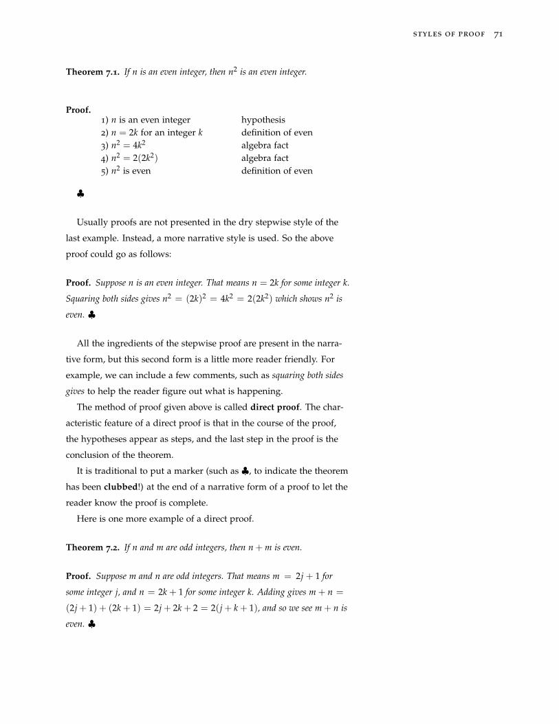
styles of proof 71
Theorem 7.1. If n is an even integer, then n2 is an even integer.
Proof.1) n is an even integer hypothesis2) n = 2k for an integer k definition of even3) n2 = 4k2 algebra fact4) n2 = 2(2k2) algebra fact5) n2 is even definition of even
♣
Usually proofs are not presented in the dry stepwise style of the
last example. Instead, a more narrative style is used. So the above
proof could go as follows:
Proof. Suppose n is an even integer. That means n = 2k for some integer k.
Squaring both sides gives n2 = (2k)2 = 4k2 = 2(2k2) which shows n2 is
even. ♣
All the ingredients of the stepwise proof are present in the narra-
tive form, but this second form is a little more reader friendly. For
example, we can include a few comments, such as squaring both sides
gives to help the reader figure out what is happening.
The method of proof given above is called direct proof. The char-
acteristic feature of a direct proof is that in the course of the proof,
the hypotheses appear as steps, and the last step in the proof is the
conclusion of the theorem.
It is traditional to put a marker (such as ♣, to indicate the theorem
has been clubbed!) at the end of a narrative form of a proof to let the
reader know the proof is complete.
Here is one more example of a direct proof.
Theorem 7.2. If n and m are odd integers, then n + m is even.
Proof. Suppose m and n are odd integers. That means m = 2j + 1 for
some integer j, and n = 2k + 1 for some integer k. Adding gives m + n =
(2j + 1) + (2k + 1) = 2j + 2k + 2 = 2(j + k + 1), and so we see m + n is
even. ♣
72 math208: discrete mathematics
7.2 Indirect proof
There are cases where a direct proof is not very convenient for one
reason or another. There are several other styles of proof, each based
on some logical equivalence.
For example, since p→ q ≡ ¬q→ ¬p, we can prove the
Theorem 7.3. p→ q
by instead giving a proof of
Theorem 7.4. ¬q→ ¬p.
In other words, we replace the requested implication with its con-
trapositive, and prove that instead. This method of proof is called
indirect proof. Here’s an example.
Theorem 7.5. If m2 is an even integer, then m is an even integer.
Proof. Suppose m is not even. Then m is odd. So m = 2k + 1 for some
integer k. Squaring both sides of that equation gives m2 = (2k + 1)2 =
4k2 + 4k + 1 = 2(2k2 + 2k) + 1, which shows m2 is not even. ♣
Notice that we gave a direct proof of the equivalent theorem: If m is
not an even integer, then m2 is not an even integer.
7.3 Proof by contradiction
Another alternative to a direct proof is proof by contradiction. In this
method the plan is to replace the requested Theorem: r (where r can
be any simple or compound proposition) with Theorem: ¬r → F,
where F is any proposition known to be false. The reason proof by
contradiction is a valid form of proof is that ¬r → F ≡ r, so that
showing ¬r → F is true is identical to showing r is true. Proofs by
contradiction can be a bit more difficult to discover than direct or
indirect proofs. The reason is that in those two types of proof, we
know exactly what the last line of our proof will be. We know where
we want to get to. But in a proof by contradiction, we only know that
we want to end up with some (any) proposition known to be false.
Typically, when writing a proof by contradiction, we experiment,
styles of proof 73
trying various logical arguments, hoping to stumble across some
false proposition, and so conclude the proof. For example, consider
the following.
Theorem 7.6.√
2 is irrational.
The plan is to replace the requested theorem with
Theorem 7.7. If√
2 is rational, then F (some fact known to be false).
And now, we may give a direct proof of this replacement theorem:
Proof. Suppose that√
2 is rational. Then there exist integers m and n with
n 6= 0, so that√
2 =mn
, withmn
in lowest terms. Squaring both sides
gives 2 =m2
n2 . Thus m2 = 2n2 and so m2 is even. Therefore m is even.
So m = 2k for some integer k. Substituting 2k for m in m2 = 2n2 shows
(2k)2 = 4k2 = 2n2. Which means that n2 = 2k2. Therefore n2 is even,
which means n is even. Now since both m and n are even, they have 2 as a
common factor. Thereforemn
is in lowest terms and it is not in lowest terms.
→←. ♣
The symbol→← (two arrows crashing into each other head on)
denotes that we have reached a fallacy (F), a statement known to be
false. It usually marks the end of a proof by contradiction.
In the next example, we will prove a proposition of the form p→ q
by contradiction. The theorem is about real numbers x and y.
Theorem 7.8. If 0 < x < y, then√
x <√
y.
Think of the statement of the theorem in the form p → q. The plan is
to replace the requested theorem with
Theorem 7.9. ¬(p→ q)→ F.
But ¬(p → q) ≡ ¬(¬p ∨ q) ≡ p ∧ ¬q. So we will actually prove
(p ∧ ¬q)→ F. In other words, we will prove (directly)
Theorem 7.10. If 0 < x < y and√
x ≥ √y, then (some fallacy).
Proof. Suppose 0 < x < y and√
x ≥ √y. Since√
x > 0,√
x√
x ≥√
x√
y, which is the same as x ≥ √xy. Also, since√
y > 0,√
y√
x ≥√
y√
y, which is the same as√
xy ≥ y. Putting x ≥ √xy and√
xy ≥ y
together, we conclude x ≥ y. Thus x < y and x ≥ y. →← ♣
74 math208: discrete mathematics
7.4 Proof by cases
The only other common style of proof is proof by cases. Let’s first
look at the justification for this proof technique. Suppose we are
asked to prove
Theorem 7.11 (Theorem X). p→ q.
We dream up some propositions, r and s, and replace the requested
theorem with three theorems:
Theorem 7.12 (Theorem XS). (1) p −→ (r ∨ s), (2) r → q, and
(3) s→ q.
The propositions r, s we dream up are called the cases. There can
be any number of cases. If we dream up three cases, then we would
have four theorems to prove, and so on. The hope is that the proofs
of these replacement theorems will be much easier than a proof of
the original theorem. 1 1 This is the divide and conquer approachto a proof.
The reason proof by cases is a valid proof technique is that
[(p −→ (r ∨ s)) ∧ (r → q) ∧ (s→ q)]→ (p→ q)
is a tautology2. Proof by cases, as for proof by contradiction, is gen- 2 Prove this!
erally a little trickier than direct and indirect proofs. In a proof by
contradiction, we are not sure exactly what we are shooting for. We
just hope some contradiction will pop up. For a proof by cases, we
have to dream up the cases to use, and it can be difficult at times to
dream up good cases.
Theorem 7.13. For any integer n, |n| ≥ n.
Proof. Suppose n is an integer. There are two cases:Either (1): n > 0, or This has the form p −→ (r ∨ s) of (1) in
Theorem 7.4.(2): n ≤ 0.
Case 1: We need to show If n > 0, then |n| ≥ n. (We will do this with a direct
proof.) Suppose n > 0. Then |n| = n. Thus |n| ≥ n is true.
Case 2: We need to show If n ≤ 0, then |n| ≥ n. (We will again use a direct
proof.) Suppose n ≤ 0. Now 0 ≤ |n|. Thus, n ≤ |n|.
So, in any case, n ≤ |n| is true, and that proves the theorem. ♣
styles of proof 75
7.5 Existence proof
A proof of a statement of the form ∃xP(x) is called an existence
proof. The proof may be constructive, meaning that the proof pro-
vides a specific example of, or at least an explicit recipe for find-
ing, an x so that P(x) is true; or the proof may be non-constructive,
meaning that it establishes the existence of x without giving a method
of actually producing an example of an x for which P(x) is true.
To give examples of each type of existence proof, let’s use a famil-
iar fact (which will be proved a little later in the course): There are
infinitely many primes. Recall that a prime is an integer greater than
1 whose only positive divisors are 1 and itself. The next two theo-
rems are contrived, but they demonstrate the ideas of constructive
and nonconstructive proofs.
Theorem 7.14. There is a prime with more than two digits.
Proof. Checking shows that 101 has no positive divisors besides 1 and itself.
Also, 101 has more than two digits. So we have produced an example of a
prime with more than two digits. ♣
That is a constructive proof of the theorem. Now, here is a non-
constructive proof of a similar theorem.
Theorem 7.15. There is a prime with more than one billion digits.
Proof. Since there are infinitely many primes, they cannot all have one
billion or fewer digits. So there must some primes with more than one billion
digits. ♣
7.6 Using a counterexample to disprove a statement
Finally, suppose we are asked to prove a theorem of the form ∀x P(x),
and for one reason or another we come to believe the proposition is
not true. The proposition can be shown to be false by exhibiting a
specific element from the domain of x for which P(x) is false. Such
an example is called a counterexample to the theorem. Let’s look at a
specific instance of the counterexample technique.
76 math208: discrete mathematics
Theorem 7.16 (not really!). For all positive integers n, n2 − n + 41 is
prime
Counterexample. To disprove the theorem, we explicitly specify a positive
integer n such that n2 − n + 41 is not prime. In fact, when n = 41, the
expression is not a prime since clearly 412 − 41 + 41 = 412 is divisible by
41. So, n = 41 is a counterexample to the proposition. ♣
An interesting fact about this example is that n = 41 is the smallest
counterexample. For n = 1, 2, · · · 40, it turns out that n2 − n + 41 is
a prime! This examples shows the danger of checking a theorem of
the form ∀x P(x) for a few (or a few billion!) values of x, finding P(x)
true for those cases, and concluding it is true for every possible value
of x.
styles of proof 77
7.7 Exercises
For the purpose of these exercises, feel free to use familiar facts and
definitions about integers. For example: Recall, an integer n is even if
n = 2k for some integer k. And, an integer n is odd if n = 2k + 1 for
some integer k.
Exercise 7.1. Give a direct proof that the sum of two even integers is even.
Exercise 7.2. Give an indirect proof that if the square of the integer n is
odd, then n is odd.
Exercise 7.3. Give a proof by contradiction that the sum of a rational
number and an irrational number is irrational.
Exercise 7.4. Give a proof by contradiction that if 5n− 1 is odd, then n is
even.
Exercise 7.5. Give a proof by cases that for integers m, n, we have |mn| =|m||n|. Hint: Consider four cases: (1) m ≥ 0 and n ≥ 0, (2) m ≥ 0 and
n < 0, (3) m < 0 and n ≥ 0, and (4) m < 0 and n < 0.
Exercise 7.6. Give an example of a predicate P(n) about positive integers
n, such that P(n) is true for every positive integer from 1 to one billion, but
which is never-the-less not true for all positive integers. (Hint: there is a
really simple choice possible for the predicate P(n).)
Exercise 7.7. In Chapter 1, exercise e), you concluded that If x = 2, then
x2 − 2x + 1 = 0 is not a proposition. Using the convention given in this
chapter, what would you say now, and why?
Exercise 7.8. Give a counterexample to the proposition Every positive
integer that ends with a 7 is a prime.

8
Relations
Two-place predicates, such as B(x, y) : x is the brother of y, play a
central role in mathematics. Such predicates can be used to describe
many basic concepts. As examples, consider the predicates given
verbally:
(1) G(x, y) : x is greater than or equal to y which compares the magni-
tudes of two values.
(2) P(x, y) : x has the same parity as y which compares the parity of two
integers.
(3) S(x, y) : x has square equal to y which relates a value to its square.
8.1 Relations
Two-place predicates are called relations, probably because of exam-
ples such as the brother of given above. To be a little more complete
about it, if P(x, y) is a two-place predicate, and the domain of dis-
course for x is the set A, and the domain of discourse for y is the
set B, then P is called a relation from A to B. When working with
relations, some new vocabulary is used. The set A (the domain of
discourse for the first variable) is called the domain of the relation,
and the set B (the domain of discourse for the second variable) is
called the codomain of the relation.
80 math208: discrete mathematics
8.2 Specifying a relation
There are several different ways to specify a relation. One way is
to give a verbal description as in the examples above. As one more
example of a verbal description of a relation, consider
E(x, y) : The word x ends with the letter y. Here the domain will be
words in English, and the codomain will the the twenty-six letters of
the alphabet. We say the ordered pair (cat, t) satisfies the relation E,
but that (dog, w) does not.
8.2.1 By ordered pairs
When dealing with abstract relations, a verbal description is not
always convenient. An alternate method is to tell what the domain
and codomain are to be, and then simply list the ordered pairs which
will satisfy the relation. For example, if A = {1, 2, 3, 4} and B =
{a, b, c, d}, then one of many possible relations from A to B would
be {(1, b), (2, c), (4, c)}. If we name this relation R, we will write
R = {(1, b), (2, c), (4, c)}. It would be tough to think of a natural
verbal description of R.
When thinking of a relation, R, as a set of ordered pairs, it is com-
mon to write aRb in place of (a, b) ∈ R. For example, using the
relation G defined above, we can convey the fact that the pair (3, 2)
satisfies the relation by writing any one of the following: (1) G(3, 2) is
true, (2) (3, 2) ∈ G, or (3) 3G2. The third choice is the preferred one
when discussing relations abstractly.
Sometimes the ordered pair representation of a relation can
be a bit cumbersome compared to the verbal description. Think
about the ordered pair form of the relation E given above: E =
{ (cat, t), (dog, g), (antidisestablishmentarianism, m), · · · }.
8.2.2 By graph
Another way represent a relation is with a graph1. Here, a graph is a 1 Here graph does not mean the sortsof graphs of lines, curves and suchdiscussed in an algebra course.diagram made up of dots, called vertices, some of which are joined
by lines, called edges. To draw a graph of a relation R from A to B,
make a column of dots, one for each element of A, and label the dots
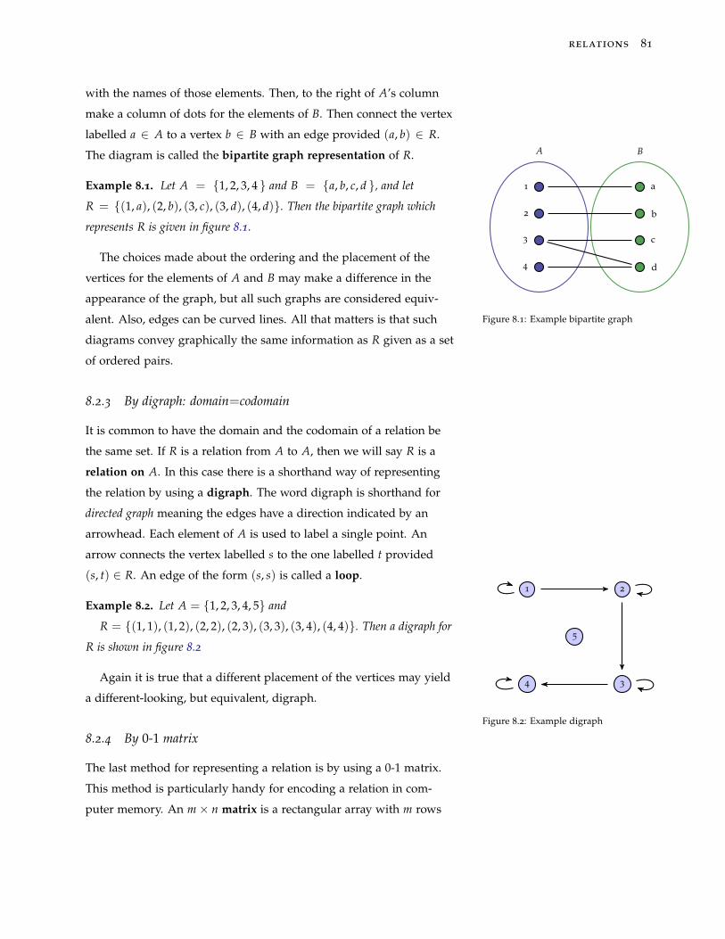
relations 81
with the names of those elements. Then, to the right of A’s column
make a column of dots for the elements of B. Then connect the vertex
labelled a ∈ A to a vertex b ∈ B with an edge provided (a, b) ∈ R.
The diagram is called the bipartite graph representation of R.
Example 8.1. Let A = {1, 2, 3, 4 } and B = {a, b, c, d }, and let
R = {(1, a), (2, b), (3, c), (3, d), (4, d)}. Then the bipartite graph which
represents R is given in figure 8.1.
1
2
3
4
a
b
c
d
A B
Figure 8.1: Example bipartite graph
The choices made about the ordering and the placement of the
vertices for the elements of A and B may make a difference in the
appearance of the graph, but all such graphs are considered equiv-
alent. Also, edges can be curved lines. All that matters is that such
diagrams convey graphically the same information as R given as a set
of ordered pairs.
8.2.3 By digraph: domain=codomain
It is common to have the domain and the codomain of a relation be
the same set. If R is a relation from A to A, then we will say R is a
relation on A. In this case there is a shorthand way of representing
the relation by using a digraph. The word digraph is shorthand for
directed graph meaning the edges have a direction indicated by an
arrowhead. Each element of A is used to label a single point. An
arrow connects the vertex labelled s to the one labelled t provided
(s, t) ∈ R. An edge of the form (s, s) is called a loop.
Example 8.2. Let A = {1, 2, 3, 4, 5} and
R = {(1, 1), (1, 2), (2, 2), (2, 3), (3, 3), (3, 4), (4, 4)}. Then a digraph for
R is shown in figure 8.2
1
5
2
34
Figure 8.2: Example digraph
Again it is true that a different placement of the vertices may yield
a different-looking, but equivalent, digraph.
8.2.4 By 0-1 matrix
The last method for representing a relation is by using a 0-1 matrix.
This method is particularly handy for encoding a relation in com-
puter memory. An m× n matrix is a rectangular array with m rows
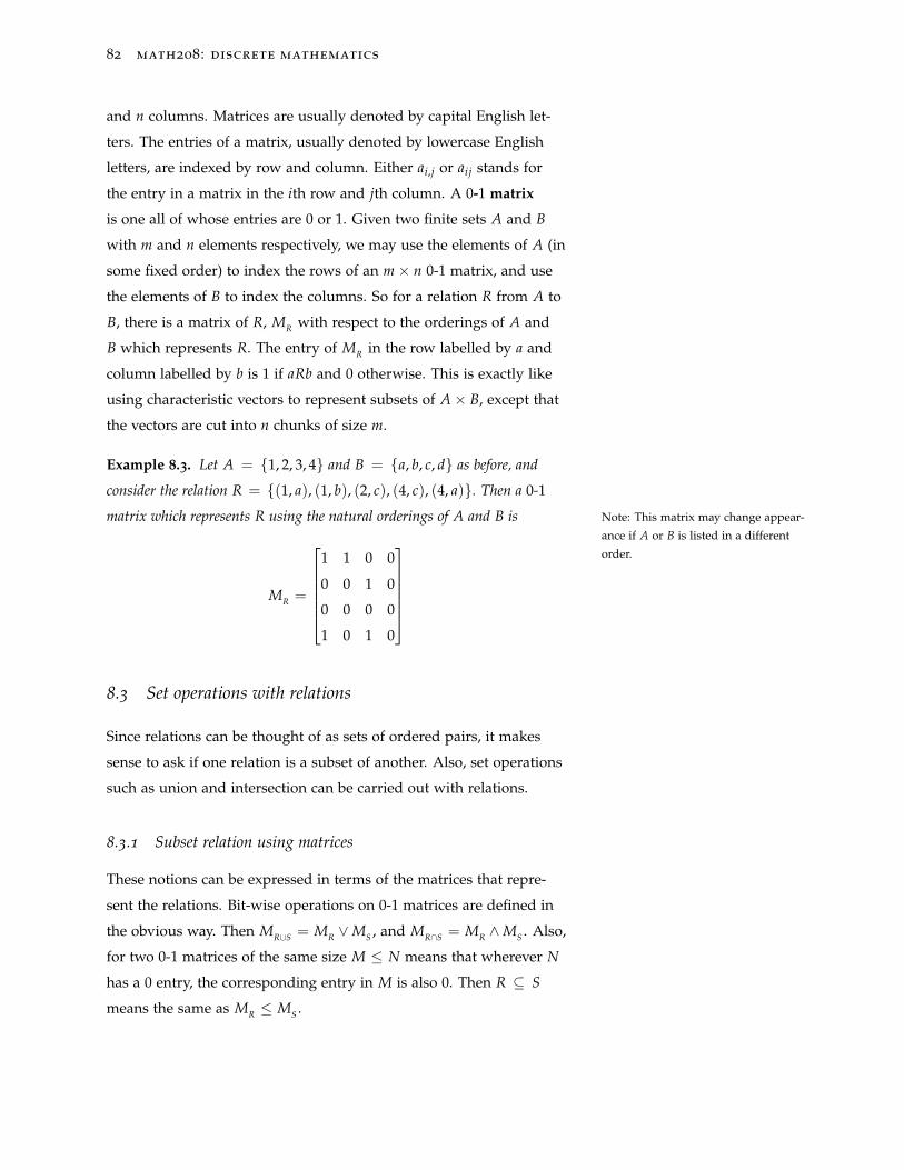
82 math208: discrete mathematics
and n columns. Matrices are usually denoted by capital English let-
ters. The entries of a matrix, usually denoted by lowercase English
letters, are indexed by row and column. Either ai,j or aij stands for
the entry in a matrix in the ith row and jth column. A 0-1 matrix
is one all of whose entries are 0 or 1. Given two finite sets A and B
with m and n elements respectively, we may use the elements of A (in
some fixed order) to index the rows of an m× n 0-1 matrix, and use
the elements of B to index the columns. So for a relation R from A to
B, there is a matrix of R, MR with respect to the orderings of A and
B which represents R. The entry of MR in the row labelled by a and
column labelled by b is 1 if aRb and 0 otherwise. This is exactly like
using characteristic vectors to represent subsets of A× B, except that
the vectors are cut into n chunks of size m.
Example 8.3. Let A = {1, 2, 3, 4} and B = {a, b, c, d} as before, and
consider the relation R = {(1, a), (1, b), (2, c), (4, c), (4, a)}. Then a 0-1
matrix which represents R using the natural orderings of A and B is Note: This matrix may change appear-
ance if A or B is listed in a different
order.
MR =
1 1 0 0
0 0 1 0
0 0 0 0
1 0 1 0
8.3 Set operations with relations
Since relations can be thought of as sets of ordered pairs, it makes
sense to ask if one relation is a subset of another. Also, set operations
such as union and intersection can be carried out with relations.
8.3.1 Subset relation using matrices
These notions can be expressed in terms of the matrices that repre-
sent the relations. Bit-wise operations on 0-1 matrices are defined in
the obvious way. Then MR∪S = MR ∨MS , and MR∩S = MR ∧MS . Also,
for two 0-1 matrices of the same size M ≤ N means that wherever N
has a 0 entry, the corresponding entry in M is also 0. Then R ⊆ S
means the same as MR ≤ MS .
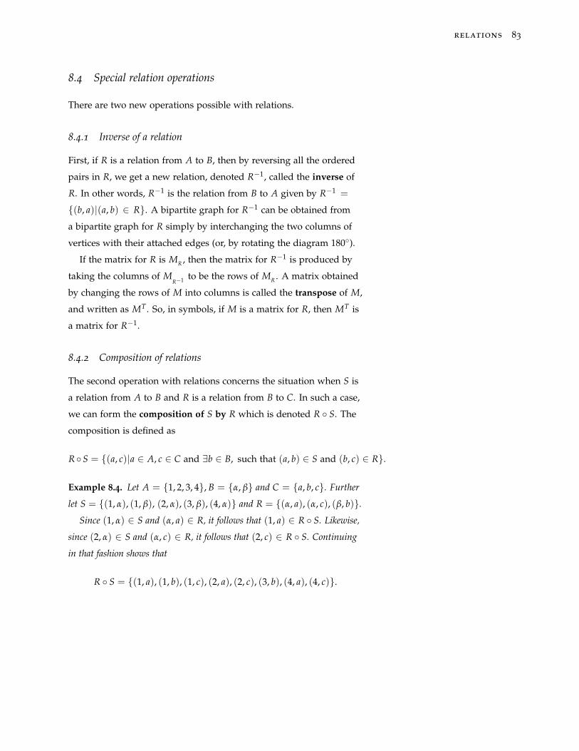
relations 83
8.4 Special relation operations
There are two new operations possible with relations.
8.4.1 Inverse of a relation
First, if R is a relation from A to B, then by reversing all the ordered
pairs in R, we get a new relation, denoted R−1, called the inverse of
R. In other words, R−1 is the relation from B to A given by R−1 =
{(b, a)|(a, b) ∈ R}. A bipartite graph for R−1 can be obtained from
a bipartite graph for R simply by interchanging the two columns of
vertices with their attached edges (or, by rotating the diagram 180◦).
If the matrix for R is MR , then the matrix for R−1 is produced by
taking the columns of MR−1 to be the rows of MR . A matrix obtained
by changing the rows of M into columns is called the transpose of M,
and written as MT . So, in symbols, if M is a matrix for R, then MT is
a matrix for R−1.
8.4.2 Composition of relations
The second operation with relations concerns the situation when S is
a relation from A to B and R is a relation from B to C. In such a case,
we can form the composition of S by R which is denoted R ◦ S. The
composition is defined as
R ◦S = {(a, c)|a ∈ A, c ∈ C and ∃b ∈ B, such that (a, b) ∈ S and (b, c) ∈ R}.
Example 8.4. Let A = {1, 2, 3, 4}, B = {α, β} and C = {a, b, c}. Further
let S = {(1, α), (1, β), (2, α), (3, β), (4, α)} and R = {(α, a), (α, c), (β, b)}.Since (1, α) ∈ S and (α, a) ∈ R, it follows that (1, a) ∈ R ◦ S. Likewise,
since (2, α) ∈ S and (α, c) ∈ R, it follows that (2, c) ∈ R ◦ S. Continuing
in that fashion shows that
R ◦ S = {(1, a), (1, b), (1, c), (2, a), (2, c), (3, b), (4, a), (4, c)}.
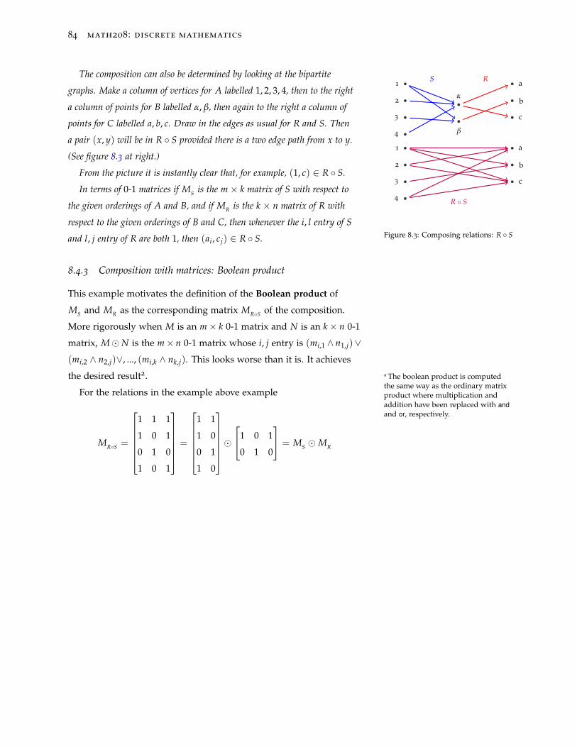
84 math208: discrete mathematics
The composition can also be determined by looking at the bipartite
graphs. Make a column of vertices for A labelled 1, 2, 3, 4, then to the right
a column of points for B labelled α, β, then again to the right a column of
points for C labelled a, b, c. Draw in the edges as usual for R and S. Then
a pair (x, y) will be in R ◦ S provided there is a two edge path from x to y.
(See figure 8.3 at right.)
1
2
3
4
α
β
a
b
c
S R
1
2
3
4
a
b
c
R ◦ S
Figure 8.3: Composing relations: R ◦ S
From the picture it is instantly clear that, for example, (1, c) ∈ R ◦ S.
In terms of 0-1 matrices if MS is the m × k matrix of S with respect to
the given orderings of A and B, and if MR is the k × n matrix of R with
respect to the given orderings of B and C, then whenever the i, l entry of S
and l, j entry of R are both 1, then (ai, cj) ∈ R ◦ S.
8.4.3 Composition with matrices: Boolean product
This example motivates the definition of the Boolean product of
MS and MR as the corresponding matrix MR◦S of the composition.
More rigorously when M is an m× k 0-1 matrix and N is an k× n 0-1
matrix, M�N is the m× n 0-1 matrix whose i, j entry is (mi,1 ∧ n1,j)∨(mi,2 ∧ n2,j)∨, ..., (mi,k ∧ nk,j). This looks worse than it is. It achieves
the desired result2. 2 The boolean product is computedthe same way as the ordinary matrixproduct where multiplication andaddition have been replaced with andand or, respectively.
For the relations in the example above example
MR◦S =
1 1 1
1 0 1
0 1 0
1 0 1
=
1 1
1 0
0 1
1 0
�1 0 1
0 1 0
= MS �MR
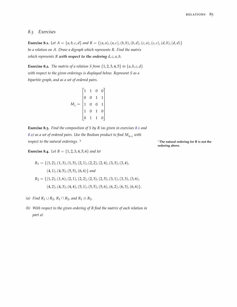
relations 85
8.5 Exercises
Exercise 8.1. Let A = {a, b, c, d} and R = {(a, a), (a, c), (b, b), (b, d), (c, a), (c, c), (d, b), (d, d)}be a relation on A. Draw a digraph which represents R. Find the matrix
which represents R with respect to the ordering d, c, a, b.
Exercise 8.2. The matrix of a relation S from {1, 2, 3, 4, 5} to {a, b, c, d}with respect to the given orderings is displayed below. Represent S as a
bipartite graph, and as a set of ordered pairs.
MS =
1 1 0 0
0 0 1 1
1 0 0 1
1 0 1 0
0 1 1 0
Exercise 8.3. Find the composition of S by R (as given in exercises 8.1 and
8.2) as a set of ordered pairs. Use the Boolean product to find MR◦S with
respect to the natural orderings. 3 3 The natural ordering for R is not theordering above.
Exercise 8.4. Let B = {1, 2, 3, 4, 5, 6} and let
R1 = {(1, 2), (1, 3), (1, 5), (2, 1), (2, 2), (2, 4), (3, 3), (3, 4),
(4, 1), (4, 5), (5, 5), (6, 6)} and
R2 = {(1, 2), (1, 6), (2, 1), (2, 2), (2, 3), (2, 5), (3, 1), (3, 3), (3, 6),
(4, 2), (4, 3), (4, 4), (5, 1), (5, 5), (5, 6), (6, 2), (6, 3), (6, 6)}.
(a) Find R1 ∪ R2, R1 ∩ R2, and R1 ⊕ R2.
(b) With respect to the given ordering of B find the matrix of each relation in
part a)

9
Properties of Relations
There are several conditions that can be imposed on a relation
R on a set A that make it useful. These requirements distinguish
those relations which are interesting for some reason from the garden
variety junk, which is, let’s face it, what most relations are.
9.1 Reflexive
A relation R on A is reflexive provided ∀a ∈ A, aRa. In plain English,
a relation is reflexive if every element of its domain is related to
itself. The relation B(x, y) : x is the brother of y is not reflexive
since no person is his own brother. On the other hand, the relation
S(m, n) : m + n is even. is a reflexive relation on the set of integers
since, for any integer m, m + m = 2m is even.
It is easy to spot a reflexive relation from its digraph: there is a
loop at every vertex. Also, a reflexive relation can be spotted quickly
from its matrix. First, let’s agree that when the matrix of a relation
on a set A is written down, the same ordering of the elements of
A is used for both the row and column designators. For a reflexive
relation, the entries on the main diagonal of its matrix will all be 1’s.
The main diagonal of a square matrix runs from the upper left corner
to the lower right corner.
88 math208: discrete mathematics
9.2 Irreflexive
The flip side of the coin from reflexive is irreflexive. A relation R on
A is irreflexive in case a�Ra for all a ∈ A. In other words, no element
of A is related to itself. The brother of relation is irreflexive. The di-
graph of an irreflexive relation contains no loops, and its matrix has
all 0’s on the main diagonal.
Actually, that discussion was a little careless. To see why, consider
the relation S(x, y) : the square of x is bigger than or equal to y.
Is this relation reflexive? The answer is: we can’t tell. The answer
depends on the domain of the relation, and we haven’t been told
what that is to be. For example, if the domain is the set N of natural
numbers, then the relation is reflexive, since n2 ≥ n for all n ∈ N.
However, if the domain is the set R of all real numbers, the relation is
not reflexive. In fact, a counterexample to the claim that S is reflexive
on R is the number 12 since
(12
)2= 1
4 , and 14 < 1 , so 1
2 �S12 . The lesson
to be learned from this example is that the question of whether a
relation is reflexive cannot be answered until the domain has been
specified. The same is true for the irreflexive condition and the other
conditions defined below. Always be sure you know the domain
before trying to determine which properties a relation satisfies.
9.3 Symmetric
A relation R on A is symmetric provided (a, b) ∈ R→ (b, a) ∈ R. An-
other way to say the same thing: R is symmetric provided R = R−1.
In words, R is symmetric provided that whenever a is related to b,
then b is related to a. Any digraph representing a symmetric rela-
tion R will have a return edge for every non-loop. Think of this as
saying the graph has no one-way streets. The matrix M of a sym-
metric relation satisfies M = MT . In this case M is symmetric about
its main diagonal in the usual geometric sense of symmetry. The
B(x, y) : x is the brother of y relation mentioned before is not sym-
metric if the domain is taken to be all people since, for example,
Donny B Marie, but Marie�B Donny. On the other hand, if we take the
domain to be all (human) males, then B is symmetric.
properties of relations 89
9.4 Antisymmetric
A relation R on A is antisymmetric if whenever (a, b) ∈ R and
(b, a) ∈ R, then a = b. In other words, the only objects that are each
related to the other are objects that are the same. For example, the
usual ≤ relation for the integers is antisymmetric since if m ≤ n and
n ≤ m, then n = m. A digraph representing an antisymmetric relation
will have all streets one-way except loops. If M is a matrix for R, then
whenever ai,j = 1 and i 6= j, aj,i = 0.
9.5 Transitive
A relation R on A is transitive if whenever (a, b) ∈ R and (b, c) ∈ R,
then (a, c) ∈ R. This can also be expressed by saying R ◦ R ⊆ R.
In a digraph for a transitive relation whenever we have a directed
path of length two from a to c through b, we must also have a direct
link from a to c. This means that any digraph of a transitive relation
has lots of triangles. This includes degenerate triangles where a, b
and c are not distinct. A matrix M of a transitive relation satisfies
M�M ≤ M. The relation ≤ on N is transitive, since from k ≤ m and
m ≤ n, we can conclude k ≤ n.
9.6 Examples
Example 9.1.
Define a relation, N on the set of all living people by the rule a N b if and
only if a, b live within one mile of each other. This relation is reflexive since
every person lives within a mile of himself. It is not irreflexive since I live
within a mile of myself. It is symmetric since if a lives within a mile of
b, then b lives within a mile of a. It is not antisymmetric since Mr. and
Mrs. Smith live within a mile of each other, but they are not the same per-
son. It is not transitive: to see why, think of the following situation (which
surely exists somewhere in the world!): there is a straight road of length 1.5
miles. Say Al lives at one end of the road, Cal lives at the other end, and Sal
lives half way between Al and Cal. Then Al N Sal and Sal N Cal, but not
Al N Cal.
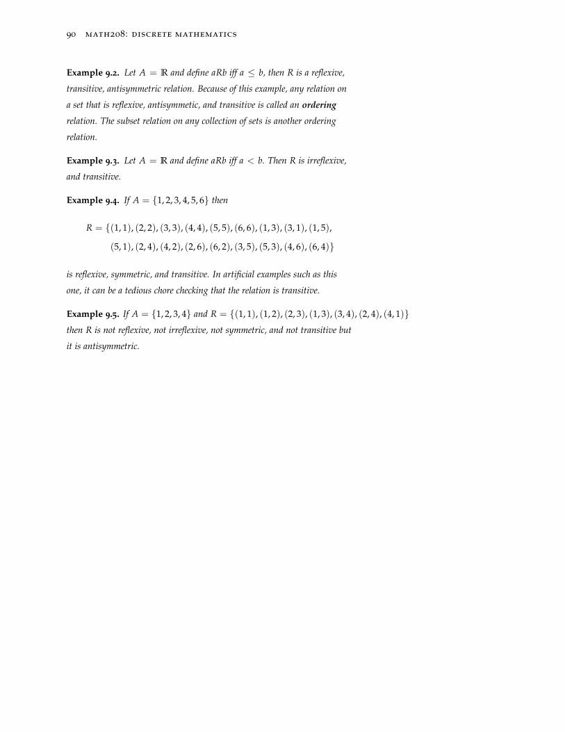
90 math208: discrete mathematics
Example 9.2. Let A = R and define aRb iff a ≤ b, then R is a reflexive,
transitive, antisymmetric relation. Because of this example, any relation on
a set that is reflexive, antisymmetic, and transitive is called an ordering
relation. The subset relation on any collection of sets is another ordering
relation.
Example 9.3. Let A = R and define aRb iff a < b. Then R is irreflexive,
and transitive.
Example 9.4. If A = {1, 2, 3, 4, 5, 6} then
R = {(1, 1), (2, 2), (3, 3), (4, 4), (5, 5), (6, 6), (1, 3), (3, 1), (1, 5),
(5, 1), (2, 4), (4, 2), (2, 6), (6, 2), (3, 5), (5, 3), (4, 6), (6, 4)}
is reflexive, symmetric, and transitive. In artificial examples such as this
one, it can be a tedious chore checking that the relation is transitive.
Example 9.5. If A = {1, 2, 3, 4} and R = {(1, 1), (1, 2), (2, 3), (1, 3), (3, 4), (2, 4), (4, 1)}then R is not reflexive, not irreflexive, not symmetric, and not transitive but
it is antisymmetric.
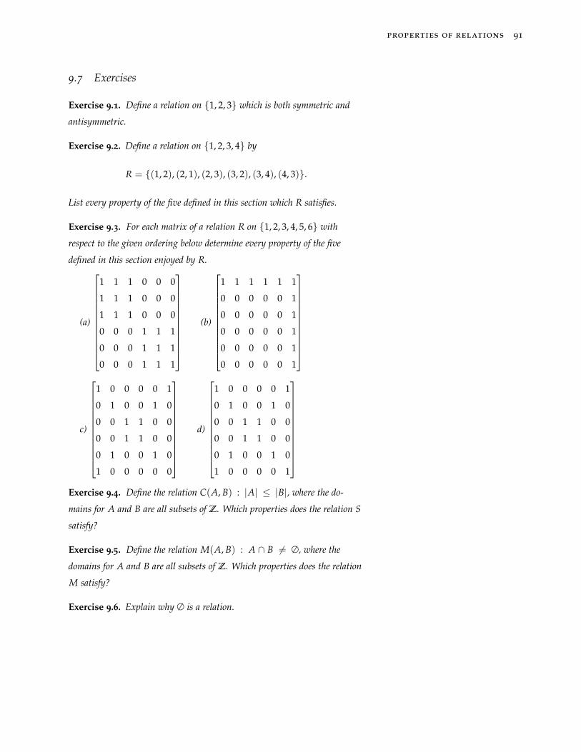
properties of relations 91
9.7 Exercises
Exercise 9.1. Define a relation on {1, 2, 3} which is both symmetric and
antisymmetric.
Exercise 9.2. Define a relation on {1, 2, 3, 4} by
R = {(1, 2), (2, 1), (2, 3), (3, 2), (3, 4), (4, 3)}.
List every property of the five defined in this section which R satisfies.
Exercise 9.3. For each matrix of a relation R on {1, 2, 3, 4, 5, 6} with
respect to the given ordering below determine every property of the five
defined in this section enjoyed by R.
(a)
1 1 1 0 0 0
1 1 1 0 0 0
1 1 1 0 0 0
0 0 0 1 1 1
0 0 0 1 1 1
0 0 0 1 1 1
(b)
1 1 1 1 1 1
0 0 0 0 0 1
0 0 0 0 0 1
0 0 0 0 0 1
0 0 0 0 0 1
0 0 0 0 0 1
c)
1 0 0 0 0 1
0 1 0 0 1 0
0 0 1 1 0 0
0 0 1 1 0 0
0 1 0 0 1 0
1 0 0 0 0 0
d)
1 0 0 0 0 1
0 1 0 0 1 0
0 0 1 1 0 0
0 0 1 1 0 0
0 1 0 0 1 0
1 0 0 0 0 1
Exercise 9.4. Define the relation C(A, B) : |A| ≤ |B|, where the do-
mains for A and B are all subsets of Z. Which properties does the relation S
satisfy?
Exercise 9.5. Define the relation M(A, B) : A ∩ B 6= ∅, where the
domains for A and B are all subsets of Z. Which properties does the relation
M satisfy?
Exercise 9.6. Explain why ∅ is a relation.
92 math208: discrete mathematics
Exercise 9.7.
(a) Let A = {1}, and consider the empty relation, ∅, on A. Which proper-
ties does ∅ satisfy?
(b) Same question as (a), but now with A = ∅.
10
Equivalence Relations
Relations capture the essence of many different mathematical
concepts. In this chapter, we will show how to put the idea of are the
same kind in terms of a special type of relation.
Before considering the formal concept of same kind let’s look at
a few simple examples. Consider the question, posed about an or-
dinary deck of 52 cards: How many different kinds of cards are there?
One possible answer is: There are 52 kinds of cards, since all the cards
are different. But another possible answer in certain circumstances
is: There are four kinds of cards (namely clubs, diamonds, hearts, and
spades). Another possible answer is: There are two kinds of cards, red
and black. Still another answer is: There are 13 kinds of cards: aces, twos,
threes, · · · , jacks, queens, and kings. Another answer, for the purpose of
many card games is: There are ten kinds of cards, aces, twos, threes, up to
nines, while tens, jacks, queens, and kings are all considered to be the same
value (usually called 10). You can certainly think of many other ways to
split the deck into a number of different kinds.
Whenever the idea of same kind is used, some properties of the ob-
jects being considered are deemed important and others are ignored.
For instance, when we think of the the deck of cards made of the 13
different ranks, ace through king, we are agreeing the the suit of the
card is irrelevant. So the jack of hearts and the jack of clubs are taken
to be the same for what ever purposes we have in mind.
94 math208: discrete mathematics
10.1 Equvialence relation
The mathematical term for same kind is equivalent. There are three
basic properties always associated with the idea of equivalence.
(1) Reflexive: Every object is equivalent to itself.
(2) Symmetric: If object a is equivalent to object b, then b is also equiv-
alent to a.
(3) Transitive: If a is equivalent to b and b is equivalent to c, then a is
equivalent to c.
To put the idea of equivalence in the context of a relation, suppose
we have a set A of objects, and a rule for deciding when two objects
in A are the same kind (equivalent) for some purpose. Then we can
define a relation E on the set A by the rule that the pair (s, t) of el-
ements of A is in the relation E if and only if s and t are the same
kind. For example, consider again the deck of cards, with two cards
considered to be the same if they have the same rank. Then a few of
the pairs in the relation E would be (ace hearts, ace spades), (three
diamonds, three clubs), (three clubs, three diamonds), (three dia-
monds, three diamonds), (king diamonds, king clubs), and so on.
Using the terminology of the previous chapter, this relation E, and
in fact any relation that corresponds to notion of equivalence, will be
reflexive, symmetric, and transitive. For that reason, any reflexive,
symmetric, transitive relation on a set A is called an equivalence
relation on A.
10.2 Equivalence class of a relation
Suppose E is an equivalence relation on a set A and that x is one par-
ticular element of A. The equivalence class of x is the set of all the
things in A that are equivalent to x. The symbol used for the equiv-
alence class of x is [x], so the definition can be written in symbols as
[x] = {y ∈ A|y E x}.For instance, think once more about the deck of cards with the
equivalence relation having the same rank. The equivalence class of the
equivalence relations 95
two of spades would be the set [2♠] = {2♣, 2♦, 2♥, 2♠}. That would
also be the equivalence class of the two of diamonds. On the other
hand, if the equivalence relation we are using for the deck is having
the same suit, then the equivalence class of the two of spades would be
[2♠] = {A♠, 2♠, 3♠, 4♠, 5♠, 6♠, 7♠, 8♠, 9♠, 10♠, J♠, Q♠, K♠}.The most important fact about the collection of different equiva-
lence classes for an equivalence relation on a set A is that they split
the set A into separate pieces. In fancier words, they partition the
set A. For example, the equivalence relation of having the same rank
splits a deck of cards into 13 different equivalence classes. In a sense,
when using this equivalence relation, there are only 13 different ob-
jects, four of each kind.
10.3 Examples
Here are a few more examples of equivalence relations.
Example 10.1. Define R on N by aRb iff a = b. In other words, equality is
an equivalence relation. If fact, this example explains the choice of name for
such relations.
Example 10.2. Let A be the set of logical propositions and define R on A by
pRq iff p ≡ q.
Example 10.3. Let A be the set of people in the world and define R on A by
aRb iff a and b are the same age in years.
Example 10.4. Let A = {1, 2, 3, 4, 5, 6} and R be the relation on A with
the matrix from exercise 3. part a) of chapter 9.
Example 10.5. Define P on Z by a P b iff a and b are both even, or both
odd. We say a and b have the same parity.
For the equivalence relation has the same rank on a set of cards in
a 52 card deck, there are 13 different equivalence classes. One of the
classes contains all the aces, another contains all the 2’s, and so on.
96 math208: discrete mathematics
Example 10.6. For the equivalence relation from example 10.5, the equiva-
lence class of 2 is the set of all even integers.
[2] = {n | 2 P n} = {n | 2 has the same parity as n }
= {n | n is even } = {· · · ,−4,−2, 0, 2, 4, · · · }
In this example, there are two different equivalence classes, the one compris-
ing all the even integers, and the other comprising all the odd integers. As
far as parity is concerned, −1232215 and 171717 are the same.
Suppose E is an equivalence relation on A. The most important
fact about equivalence classes is that every element of A belongs to
exactly one equivalence class. Let’s prove that.
Theorem 10.7. Let E be an equivalence relation on a set A, and let a ∈ A.
Then there is exactly one equivalence class to which a belongs.
Proof. Let E be an equivalence relation on a set A, and suppose a ∈ A.
Since E is reflexive, a E a, and so a ∈ [a] is true. That proves that a is in
at least one equivalence class. To complete the proof, we need to show that if
a ∈ [b] then [b] = [a].
Now, stop and think: Here is what we know:
(1) E is an equivalence relation on A,
(2) a ∈ [b], and
(3) the definition of equivalence class.
Using those three pieces of information, we need to show the two sets [a] and
[b] are equal. Now, to show two sets are equal, we show they have the same
elements. In other words, we want to prove
(1) If c ∈ [a], then c ∈ [b], and For homework, you will complete the
proof of this theorem by doing part (1).(2) If c ∈ [b], then c ∈ [a].
Let’s give a direct proof of (2).
Suppose c ∈ [b]. Then, according to the definition of [b], c E b. The goal
is to end up with So c ∈ [a]. Now, we know a ∈ [b], and that means a E b.
Since E is symmetric and a E b, it follows that b E a. Now we have c E b and
b E a. Since E is transitive, we can conclude c E a, which means c ∈ [a] as
we hoped to show. That proves (2). ♣
equivalence relations 97
10.4 Partitions
Definition 10.8. A partition of a set A is a collection of nonempty,
pairwise disjoint subsets of A, so that A is the union of the subsets
in the collection. So for example {{1, 2, 3} {4, 5, 6}} is a partition of
{1, 2, 3, 4, 5, 6}. The subsets forming a partition are called the parts of
the partition.
So to express the meaning of theorem 10.7 above in different
words: The different equivalence classes of an equivalence relation
on a set partition the set into nonempty disjoint pieces. More briefly:
the equivalence classes of E partition A.
10.5 Digraph of an equivalence relation
The fact that an equivalence relation partitions the underlying set
is reflected in the digraph of an equivalence relation. If we pick an
equivalence class [a] of an equivalence relation E on a finite set A
and we pick b ∈ [a], then b E c for all c ∈ [a]. This is true since
a E b implies b E a and if a E c, then transitivity fills in b E c. So in any
digraph for E every vertex of [a] is connected to every other vertex
in [a] (including itself) by a directed edge. Also no vertex in [a] is
connected to any vertex in A − [a]. So the digraph of E consists of
separate components, one for each distinct equivalence class, where
each component contains every possible directed edge.
10.6 Matrix representation of an equivalence relation
In terms of a matrix representation of an equivalence relation E on
a finite set A of size n, let the distinct equivalence classes have size
k1, k2, ...kr, where k1 + k2 + ... + kr = n. Next list the elements of A as
a1,1, ..., ak1,1, a1,2, ..., ak2,2, ....., a1,r, ..., akr ,r where the ith equivalence class
is {a1,i, ..., aki ,i}. Then the matrix for R with respect to this ordering is
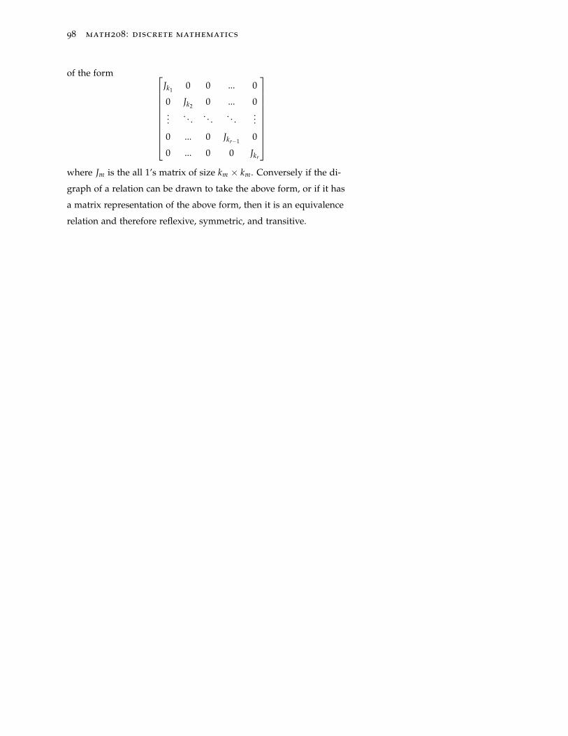
98 math208: discrete mathematics
of the form
Jk1 0 0 ... 0
0 Jk2 0 ... 0...
. . . . . . . . ....
0 ... 0 Jkr−1 0
0 ... 0 0 Jkr
where Jm is the all 1’s matrix of size km × km. Conversely if the di-
graph of a relation can be drawn to take the above form, or if it has
a matrix representation of the above form, then it is an equivalence
relation and therefore reflexive, symmetric, and transitive.
equivalence relations 99
10.7 Exercises
Exercise 10.1. Let A be the set of people alive on earth. For each relation
defined below, determine if it is an equivalence relation on A. If it is, de-
scribe the equivalence classes. If it is not, determine which properties of an
equivalence relation fail.
(a) a H b←→ a and b are the same height.
(b) a G b←→ a and b have a common grandparent.
(c) a L b←→ a and b have the same last name.
(d) a N b←→ a and b have a name (first name or last name) in common.
(e) a W b←→ a and b were born less than a day apart.
Exercise 10.2. Let E be an equivalence relation on a set A, and let a, b ∈ A.
Prove that either [a] = [b] or else [a] ∩ [b] = ∅.
Exercise 10.3. Consider the relation B(x, y) : x is the brother of y on the
set, M, of living human males. Is this an equivalence relation on M?
Exercise 10.4. Let A = {1, 2, 3, 4, 5, 6, 7, 8}. Form a partition of A using
{1, 2, 4}, {3, 5, 7}, and {6, 8}. These are the equivalence classes for an
equivalence relation, E, on A.
(a) Draw a digraph of E.
(b) Determine a 0-1 matrix of E.
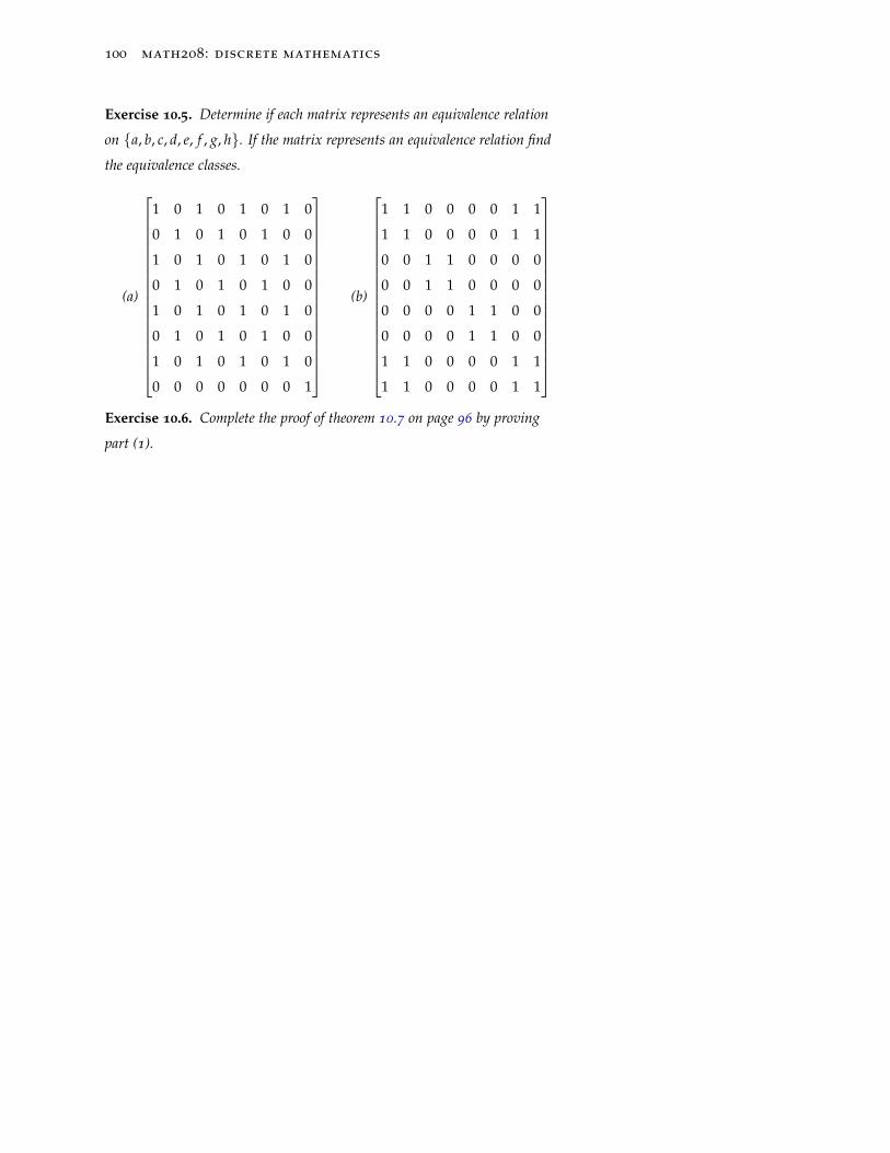
100 math208: discrete mathematics
Exercise 10.5. Determine if each matrix represents an equivalence relation
on {a, b, c, d, e, f , g, h}. If the matrix represents an equivalence relation find
the equivalence classes.
(a)
1 0 1 0 1 0 1 0
0 1 0 1 0 1 0 0
1 0 1 0 1 0 1 0
0 1 0 1 0 1 0 0
1 0 1 0 1 0 1 0
0 1 0 1 0 1 0 0
1 0 1 0 1 0 1 0
0 0 0 0 0 0 0 1
(b)
1 1 0 0 0 0 1 1
1 1 0 0 0 0 1 1
0 0 1 1 0 0 0 0
0 0 1 1 0 0 0 0
0 0 0 0 1 1 0 0
0 0 0 0 1 1 0 0
1 1 0 0 0 0 1 1
1 1 0 0 0 0 1 1
Exercise 10.6. Complete the proof of theorem 10.7 on page 96 by proving
part (1).
11
Functions and Their Properties
In algebra, functions are thought of as formulas such as f (x) =
x2 where x is any real number. This formula gives a rule that de-
scribes how to determine one number if we are handed some number
x. So, for example, if we are handed x = 2, the function f says that
determines the value 4, and if we are handed 0, f says that deter-
mines 0. There is one condition that, by mutual agreement, such
a function rule must obey to earn the title function: the rule must
always determine exactly one value for each (reasonable) value it is
handed. Of course, for the example above, x = blue isn’t a reasonable
choice for x, so f doesn’t determine a value associated with blue. The
domain of this function is all real numbers.
Instead of thinking of a function as a formula, we could think of
a function as any rule which determines exactly one value for every
element of a set A. For example, suppose W is the set of all words in
English, and consider the rule, I, which associates with each word, w,
the first letter of w. Then I(cat) = c, I(dog) = d, I(a) = a, and so on.
Notice that for each word w, I always determines exactly one value,
so it meets the requirement of a function mentioned above. Notice
that for the same set of all English words, the rule T(w) is the third
letter of the word w is not a function since, for example, T(be) has no
value.
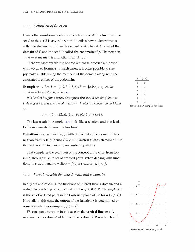
102 math208: discrete mathematics
11.1 Definition of function
Here is the semi-formal definition of a function: A function from the
set A to the set B is any rule which describes how to determine ex-
actly one element of B for each element of A. The set A is called the
domain of f , and the set B is called the codomain of f . The notation
f : A→ B means f is a function from A to B.
There are cases where it is not convenient to describe a function
with words or formulas. In such cases, it is often possible to sim-
ply make a table listing the members of the domain along with the
associated member of the codomain.
Example 11.1. Let A = {1, 2, 3, 4, 5, 6}, B = {a, b, c, d, e} and let
f : A→ B be specified by table 11.1
x f (x)
1 a
2 a
3 c
4 b
5 d
6 eTable 11.1: A simple function
It is hard to imagine a verbal description that would act like f , but the
table says it all. It is traditional to write such tables in a more compact form
as
f = { (1, a), (2, a), (3, c), (4, b), (5, d), (6, e) }.
The last result in example 11.1 looks like a relation, and that leads
to the modern definition of a function:
Definition 11.2. A function, f , with domain A and codomain B is a
relation from A to B (hence f ⊆ A× B) such that each element of A is
the first coordinate of exactly one ordered pair in f .
That completes the evolution of the concept of function from for-
mula, through rule, to set of ordered pairs. When dealing with func-
tions, it is traditional to write b = f (a) instead of (a, b) ∈ f .
11.2 Functions with discrete domain and codomain
In algebra and calculus, the functions of interest have a domain and a
codomain consisting of sets of real numbers, A, B ⊆ R. The graph of f
is the set of ordered pairs in the Cartesian plane of the form (x, f (x)).
Normally in this case, the output of the function f is determined by
some formula. For example, f (x) = x2.
y = x2
x
y
1 2 3
1
2
3
4
Figure 11.1: Graph of y = x2
We can spot a function in this case by the vertical line test. A
relation from a subset A of R to another subset of R is a function if
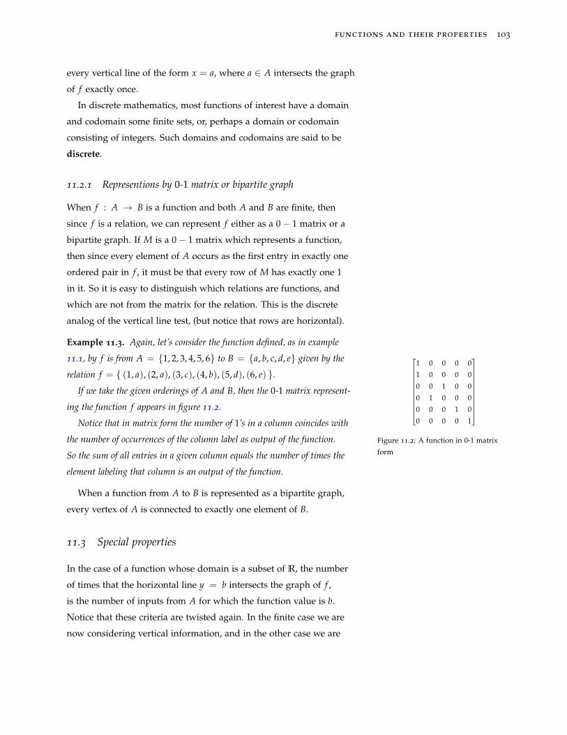
functions and their properties 103
every vertical line of the form x = a, where a ∈ A intersects the graph
of f exactly once.
In discrete mathematics, most functions of interest have a domain
and codomain some finite sets, or, perhaps a domain or codomain
consisting of integers. Such domains and codomains are said to be
discrete.
11.2.1 Representions by 0-1 matrix or bipartite graph
When f : A → B is a function and both A and B are finite, then
since f is a relation, we can represent f either as a 0− 1 matrix or a
bipartite graph. If M is a 0− 1 matrix which represents a function,
then since every element of A occurs as the first entry in exactly one
ordered pair in f , it must be that every row of M has exactly one 1
in it. So it is easy to distinguish which relations are functions, and
which are not from the matrix for the relation. This is the discrete
analog of the vertical line test, (but notice that rows are horizontal).
Example 11.3. Again, let’s consider the function defined, as in example
11.1, by f is from A = {1, 2, 3, 4, 5, 6} to B = {a, b, c, d, e} given by the
relation f = { (1, a), (2, a), (3, c), (4, b), (5, d), (6, e) }.If we take the given orderings of A and B, then the 0-1 matrix represent-
ing the function f appears in figure 11.2.
1 0 0 0 0
1 0 0 0 0
0 0 1 0 0
0 1 0 0 0
0 0 0 1 0
0 0 0 0 1
Figure 11.2: A function in 0-1 matrix
form
Notice that in matrix form the number of 1’s in a column coincides with
the number of occurrences of the column label as output of the function.
So the sum of all entries in a given column equals the number of times the
element labeling that column is an output of the function.
When a function from A to B is represented as a bipartite graph,
every vertex of A is connected to exactly one element of B.
11.3 Special properties
In the case of a function whose domain is a subset of R, the number
of times that the horizontal line y = b intersects the graph of f ,
is the number of inputs from A for which the function value is b.
Notice that these criteria are twisted again. In the finite case we are
now considering vertical information, and in the other case we are
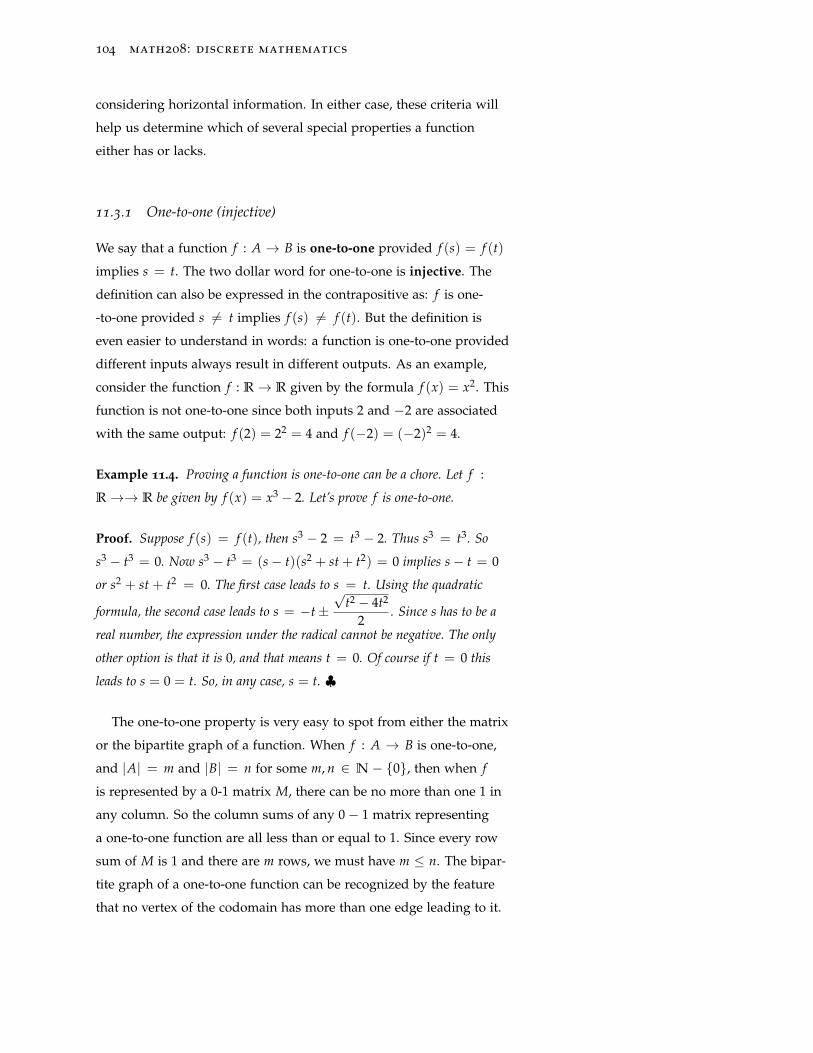
104 math208: discrete mathematics
considering horizontal information. In either case, these criteria will
help us determine which of several special properties a function
either has or lacks.
11.3.1 One-to-one (injective)
We say that a function f : A → B is one-to-one provided f (s) = f (t)
implies s = t. The two dollar word for one-to-one is injective. The
definition can also be expressed in the contrapositive as: f is one-
-to-one provided s 6= t implies f (s) 6= f (t). But the definition is
even easier to understand in words: a function is one-to-one provided
different inputs always result in different outputs. As an example,
consider the function f : R→ R given by the formula f (x) = x2. This
function is not one-to-one since both inputs 2 and −2 are associated
with the same output: f (2) = 22 = 4 and f (−2) = (−2)2 = 4.
Example 11.4. Proving a function is one-to-one can be a chore. Let f :
R→→ R be given by f (x) = x3 − 2. Let’s prove f is one-to-one.
Proof. Suppose f (s) = f (t), then s3 − 2 = t3 − 2. Thus s3 = t3. So
s3 − t3 = 0. Now s3 − t3 = (s− t)(s2 + st + t2) = 0 implies s− t = 0
or s2 + st + t2 = 0. The first case leads to s = t. Using the quadratic
formula, the second case leads to s = −t±√
t2 − 4t2
2. Since s has to be a
real number, the expression under the radical cannot be negative. The only
other option is that it is 0, and that means t = 0. Of course if t = 0 this
leads to s = 0 = t. So, in any case, s = t. ♣
The one-to-one property is very easy to spot from either the matrix
or the bipartite graph of a function. When f : A → B is one-to-one,
and |A| = m and |B| = n for some m, n ∈ N− {0}, then when f
is represented by a 0-1 matrix M, there can be no more than one 1 in
any column. So the column sums of any 0− 1 matrix representing
a one-to-one function are all less than or equal to 1. Since every row
sum of M is 1 and there are m rows, we must have m ≤ n. The bipar-
tite graph of a one-to-one function can be recognized by the feature
that no vertex of the codomain has more than one edge leading to it.
functions and their properties 105
11.3.2 Onto (surjective)
We say that a function f : A → B is onto, or surjective, if every
element of B equals f (a) for some a ∈ A. Consequently any matrix
representing an onto function has each column sum at least one, and
thus m ≥ n. In terms of bipartite graphs, for an onto function, every
element of the codomain has at least one edge leading to it.
As an example, consider again the function L from all English
words to the set of letters of the alphabet defined by the rule L(w)
is the last letter of the word w. This function is not one-to-one since,
for example, L(cat) = L(mutt), so two different members of the
domain of L are associated with the same member (namely t) of the
codomain. However, L is onto. We could prove that by making a
list of twenty-six words, one ending with a, one ending with b, · · · ,one ending with z. (Only the letters j and q might take more than a
moment’s thought.)
11.3.3 Bijective
A function f : A → B which is both one-to-one and onto is called
bijective. In the matrix of a bijection, every column has exactly one
1 and every row has exactly one 1. So the number of rows must
equal the number of columns. In other words, if there is a bijection
f : A → B, where A is a finite set, then A and B have the same
number of elements. In such a case we will say the sets have the
same cardinality or that they are equinumerous, and write that as
|A| = |B|. The general definition (whether A and B are finite or not)
is:
Definition 11.5. A and B are equinumerous provided there exists a
bijection from A to B.
Notice that for finite sets with the same number of elements, A, B,
any one-to-one function must be onto and vice versa. This is not true
for infinite sets. For example the function f : Z → Z by f (m) = 2m
is one-to-one, but not onto, since f (n) = 1 is impossible for any n.
On the other hand, the function g : Z → Z given by the rule g(n) is
the smallest integer that is greater than or equal to n2 is onto, but not
106 math208: discrete mathematics
one-to-one. As examples, g(6) = 3 and g(−5) = −2. This function is
onto since clearly g(2n) = n for any integer n, so every element of the
codomain has at least one edge leading to it. But g(1) = g(2) = 1, so
g is not one-to-one.
11.4 Composition of functions
Since functions are relations, the composition of a function g : A→ B
by a function f : B → C, makes sense. As usual, this is written as
f ◦ g : A → C, but that’s a little presumptive since it seems to assume
that f ◦ g really is a function.
Theorem 11.6. If g : A→ B and f : B→ C, then f ◦ g is a function.
Proof. We need to show that for each a ∈ A there is exactly one c ∈ C
such that (a, c) ∈ f ◦ g. So suppose a ∈ A. since g : A → B, there is
some b ∈ B with (a, b) ∈ g. Since f : B → C, there is a c ∈ C such that
(b, c) ∈ f . So, by the definition of composition, (a, c) ∈ f ◦ g. That proves
there is at least one c ∈ C with (a, c) ∈ f ◦ g. To complete the proof, we
need to show that there is only one element of C that f ◦ g pairs up with a.
So, suppose that (a, c) and (a, d) are both in f ◦ g. We need to show c = d.
Since (a, c) and (a, d) are both in f ◦ g, there must be elements s, t ∈ B such
that (a, s) ∈ g and (s, c) ∈ f , and also (a, t) ∈ g and (t, d) ∈ f . Now, since
g is a function, and both (a, s) and (a, t) are in g, we can conclude s = t. So
when we write (t, d) ∈ f , we might as well write (s, d) ∈ f . So we know
(s, c) and (s, d) are both in f . As f is a function, we can conclude c = d. ♣
If g : A → B and f : B → C, and (a, b) ∈ g and (b, c) ∈ f , then
(a, c) ∈ f ◦ g. Another way to write that is g(a) = b and f (b) = c.
So c = f (b) = f (g(a)). That last expression look like the familiar
formula for the composition of functions found in algebra texts:
( f ◦ g)(x) = f (g(x)).
11.5 Invertible discrete functions
When f : A → B is a function, we can form the relation f−1 from
B to A. But f−1 might not be a function. For example, suppose f :
functions and their properties 107
{a, b} → {1, 2} is f = {(a, 1), (b, 1)}. Then f−1 = {(1, a), (1, b)},definitely not a function.
If in fact f−1 is a function, then for all a ∈ A with b = f (a), we
have f−1(b) = a so ( f−1 ◦ f )(a) = f−1( f (a)) = f−1(b) = a, ∀a ∈ A.
Similarly ( f ◦ f−1)(b) = b, ∀b ∈ B. In this case we say f is invertible.
Another way to say the same thing: the inverse of a function f :
A → B is a function g : B → A which undoes the operation of f .
As a particular example, consider the function f : Z → Z given
by the formula f (n) = n + 3. In words, f is the add 3 function.
The operation which undoes the effect of f is clearly the subtract 3
function. That is, f−1(n) = n− 3.
For any set, S, define 1S : S → S by 1S(x) = x for every x ∈ S.
In other words, 1S = {(x, x) | x ∈ S}. The function 1S is called the
identity function on S. So the computations above show f−1 ◦ f =
1A and f ◦ f−1 = 1B.
Theorem 11.7. A function f : A→ B is invertible iff f is bijective.
Proof. First suppose that f : A → B is invertible. Then f−1 : B → A
exists. If f (a1) = f (a2), then since f−1 is a function, a1 = f−1( f (a1)) =
f−1( f (a2)) = a2. Thus f is one-to-one. Also if b ∈ B with f−1(b) = a,
then f (a) = f ( f−1(b)) = b. So f is onto. Since f is one-to-one and onto, f
is bijective.
Now suppose that f is bijective, and let b ∈ B. Since f is onto, we have
some a ∈ A with f (a) = b. If e ∈ A with f (e) = b, then e = a since
f is one-to-one. Thus b is the first entry in exactly one ordered pair in the
inverse relation f−1. Whence, f−1 is a function. ♣
Do not make the error1of confusing inverses and reciprocals when1
�
(Danger ahead!) They are entirelydifferent things.dealing with functions. The reciprocal of f : Z → Z given by the
formula f (n) = n + 3 is1
f (n)=
1n + 3
which is not the inverse
function for f . For example f (0) = 3, but the reciprocal of f does
not convert 3 back into 0, instead the reciprocal associates 16 with 3.
In fact, there are other problems with the reciprocal: it doesn’t even
make sense when n = −3 since that would give a division by 0,
which is undefined. So, be very careful when working with functions
not to confuse the words reciprocal and inverse.
108 math208: discrete mathematics
11.6 Characteristic functions
The characteristic vector (see section 6.10) of a set may be used to
define a special 0-1 function representing the given set.
Example 11.8. Let U be a finite universal set with n elements ordered
u1, ..., un. Let Bn denote all binary strings of length n. The characteristic
function χ : P(U ) → Bn, which takes a subset A to its characteristic
vector is bijective. Thus there is no danger of miscomputation. We can either
manipulate subsets of U using set operations and then represent the result
as a binary vector or we can represent the subsets as binary vectors and
manipulate the vectors with appropriate bit string operations. We’ll get
exactly the same answer either way.
The process in example 11.8 allows us therefore to translate any
set theory problem with finite sets into the world of 0’s and 1’s. This
is the essence of computer science.
functions and their properties 109
11.7 Exercises
Exercise 11.1. Let A = {1, 2, 3, 4, 5, 6}. In each case, give an example of a
function f : A → A with the indicated properties, or explain why no such
function exists.
(a) f is bijective, but not 1A.
(b) f is neither one-to-one nor onto.
(c) f is one-to-one, but not onto.
(d) f is onto, but not one-to-one.
Exercise 11.2. Repeat exercise 11.1, with the set A = N.
Exercise 11.3. Prove or give a counterexample:
If E is an equivalence relations on a set A, then E ◦ E is an equivalence
relation on A.
Exercise 11.4. Suppose g : A → B and f : B → C are both one-to-one.
Prove f ◦ g is one-to-one.

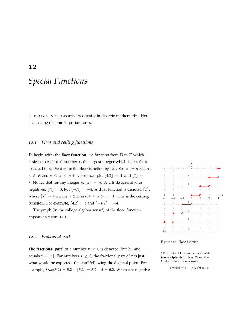
12
Special Functions
Certain functions arise frequently in discrete mathematics. Here
is a catalog of some important ones.
12.1 Floor and ceiling functions
To begin with, the floor function is a function from R to Z which
assigns to each real number x, the largest integer which is less than
or equal to x. We denote the floor function by bxc. So bxc = n means
n ∈ Z and n ≤ x < n + 1. For example, b4.2c = 4, and b7c =
7. Notice that for any integer n, bnc = n. Be a little careful with
negatives: bπc = 3, but b−πc = −4. A dual function is denoted dxe,where dxe = n means n ∈ Z and n ≥ x > n− 1. This is the ceiling
function. For example, d4.2e = 5 and d−4.2e = −4.
x
y
−3 −2 −1 0 1 2 3
−4
−3
−2
−1
1
2
3
Figure 12.1: Floor function
The graph (in the college algebra sense!) of the floor function
appears in figure 12.1.
12.2 Fractional part
The fractional part1 of a number x ≥ 0 is denoted f rac(x) and1 This is the Mathematica and Wol-fram/Alpha definition. Often, theGraham definition is used:
f rac(x) = x− bxc, for all x.
equals x − bxc. For numbers x ≥ 0, the fractional part of x is just
what would be expected: the stuff following the decimal point. For
example, f rac(5.2) = 5.2− b5.2c = 5.2− 5 = 0.2. When x is negative
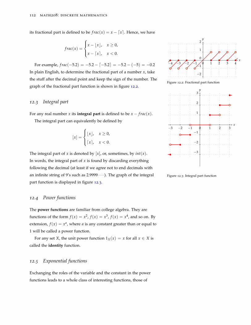
112 math208: discrete mathematics
its fractional part is defined to be f rac(x) = x− dxe. Hence, we have
f rac(x) =
x− bxc, x ≥ 0,
x− dxe, x < 0.x
y
−4 −3 −2 −1 0 1 2 3 4
−2
−1
0
1
2
Figure 12.2: Fractional part function
For example, f rac(−5.2) = −5.2− d−5.2e = −5.2− (−5) = −0.2
In plain English, to determine the fractional part of a number x, take
the stuff after the decimal point and keep the sign of the number. The
graph of the fractional part function is shown in figure 12.2.
12.3 Integral part
For any real number x its integral part is defined to be x− f rac(x).
x
y
−3 −2 −1 0 1 2 3
−3
−2
−1
1
2
3
Figure 12.3: Integral part function
The integral part can equivalently be defined by
[x] =
bxc, x ≥ 0,
dxe, x < 0.
The integral part of x is denoted by [x], or, sometimes, by int(x).
In words, the integral part of x is found by discarding everything
following the decimal (at least if we agree not to end decimals with
an infinite string of 9’s such as 2.9999 · · · ). The graph of the integral
part function is displayed in figure 12.3.
12.4 Power functions
The power functions are familiar from college algebra. They are
functions of the form f (x) = x2, f (x) = x3, f (x) = x4, and so on. By
extension, f (x) = xa, where a is any constant greater than or equal to
1 will be called a power function.
For any set X, the unit power function 1X(x) = x for all x ∈ X is
called the identity function.
12.5 Exponential functions
Exchanging the roles of the variable and the constant in the power
functions leads to a whole class of interesting functions, those of
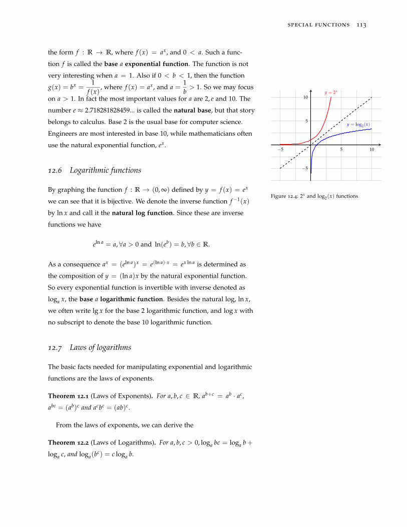
special functions 113
the form f : R → R, where f (x) = ax, and 0 < a. Such a func-
tion f is called the base a exponential function. The function is not
very interesting when a = 1. Also if 0 < b < 1, then the function
g(x) = bx =1
f (x), where f (x) = ax, and a =
1b> 1. So we may focus
on a > 1. In fact the most important values for a are 2, e and 10. The
number e ≈ 2.718281828459... is called the natural base, but that story
belongs to calculus. Base 2 is the usual base for computer science.
Engineers are most interested in base 10, while mathematicians often
use the natural exponential function, ex. −5 5 10
−5
5
10y = 2x
y = log2(x)
Figure 12.4: 2x and log2(x) functions
12.6 Logarithmic functions
By graphing the function f : R → (0, ∞) defined by y = f (x) = ex
we can see that it is bijective. We denote the inverse function f−1(x)
by ln x and call it the natural log function. Since these are inverse
functions we have
eln a = a, ∀a > 0 and ln(eb) = b, ∀b ∈ R.
As a consequence ax = (eln a)x = e(ln a)·x = ex ln a is determined as
the composition of y = (ln a)x by the natural exponential function.
So every exponential function is invertible with inverse denoted as
loga x, the base a logarithmic function. Besides the natural log, ln x,
we often write lg x for the base 2 logarithmic function, and log x with
no subscript to denote the base 10 logarithmic function.
12.7 Laws of logarithms
The basic facts needed for manipulating exponential and logarithmic
functions are the laws of exponents.
Theorem 12.1 (Laws of Exponents). For a, b, c ∈ R, ab+c = ab · ac,
abc = (ab)c and acbc = (ab)c.
From the laws of exponents, we can derive the
Theorem 12.2 (Laws of Logarithms). For a, b, c > 0, loga bc = loga b +
loga c, and loga(bc) = c loga b.
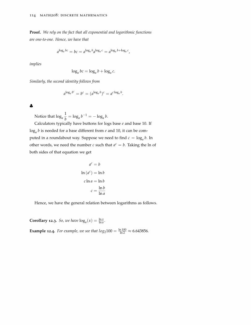
114 math208: discrete mathematics
Proof. We rely on the fact that all exponential and logarithmic functions
are one-to-one. Hence, we have that
aloga bc = bc = aloga baloga c = aloga b+loga c,
implies
loga bc = loga b + loga c.
Similarly, the second identity follows from
aloga bc= bc = (aloga b)c = ac loga b.
♣
Notice that loga1b= loga b−1 = − loga b.
Calculators typically have buttons for logs base e and base 10. If
loga b is needed for a base different from e and 10, it can be com-
puted in a roundabout way. Suppose we need to find c = loga b. In
other words, we need the number c such that ac = b. Taking the ln of
both sides of that equation we get
ac = b
ln (ac) = ln b
c ln a = ln b
c =ln bln a
Hence, we have the general relation between logarithms as follows.
Corollary 12.3. So, we have loga(x) = ln xln a .
Example 12.4. For example, we see that log2100 = ln 100ln 2 ≈ 6.643856.
special functions 115
12.8 Exercises
Exercise 12.1. In words, bxc is the largest integer less than or equal to
x. Complete the sentence: In words,dxe is the smallest . . . . . . Draw a
(college algebra) graph of f (x) = dxe.
Exercise 12.2. Draw a (college algebra) graph of f (x) = b2x− 1c.
Exercise 12.3. Draw a (college algebra) graph of f (x) = 2bx− 1c.
Exercise 12.4. Let f (x) = 18x and let g(x) =x3
2. Sketch the graphs of
f and g for x ≥ 1 on the same set of axes. Notice that the graph g is lower
then the graph of f when x = 1, but it is above the graph of f when x = 9.
Where does g cross the graph of f (in other words, where does g catch up
with f )?
Exercise 12.5. Let f (x) = 4x5 and let g(x) = 2x. For values of x ≥ 1 it
appears that the graph of g is lower than the graph of f . Does g ever catch
up with f , or does f always stay ahead of g?
Exercise 12.6. The xy button on your calculator is broken. Show how can
you approximate 2√
2 with your calculator anyhow.

13
Sequences and Summation
A sequence is a list of numbers in a specific order. For example,
the positive integers 1, 2, 3, · · · is a sequence, as is the list 4, 3, 3, 5,
4, 4, 3, 5, 5, 4 of the number of letters in the English words of the ten
digits in order zero, one, · · · , nine. Actually, the first is an example
of an infinite sequence, the second is a finite sequence. The first se-
quence goes on forever; there is no last number. The second sequence
eventually comes to a stop. In fact the second sequence has only ten
items. A term of a sequence is one of the numbers that appears in
the sequence. The first term is the first number in the list, the second
term is the second number in the list, and so on.
13.1 Specifying sequences
A more general way to think of a sequence is as a function from
some subset of Z having a least member (in most cases either { 0, 1, 2, · · · }or { 1, 2, · · · }) with codomain some arbitrary set. In most mathemat- Computer science texts use the former
and elementary math application texts
use the later. Mathematicians use any
such well-ordered domain set.
ics courses the codomain will be a set of numbers, but that isn’t nec-
essary. For example, consider the finite sequence of initial letters of
the words in the previous paragraph: a, s, i, a, l, o, n, · · · , a, s, o. If the
letter L is used to denote the function that forms this sequence, then
L(1) = a, L(2) = s, and so on.
118 math208: discrete mathematics
13.1.1 Defining a Sequence With a Formula
The examples of sequences given so far were described in words, but
there are other ways to tell what objects appear in the sequence. One
way is with a formula. For example, let s(n) = n2, for n = 1, 2, 3, · · · .As the values 1, 2, 3 and so on are plugged into s(n) in succession,
the infinite sequence 1, 4, 9, 16, 25, 36, · · · is built up. It is traditional
to write sn (or tn, etc) instead of s(n) when describing the terms of
a sequence, so the formula above would usually be seen as sn = n2.
Read that as s sub n equals n2. When written this way, the n in the sn
is called a subscript or index. The subscript of s173 is 173.
Example 13.1. What is the 50th term of the sequence defined by the formula
sj =j + 1j + 2
, where j = 1, 2, 3, . . .? We see that
s50 =5152
.
Example 13.2. What is the 50th term of the sequence defined by the formula
tk =k + 1k + 2
, where k = 0, 1, 2, 3, . . .? Since the indicies start at 0, the 50th
term will be t49:
t49 =5051
.
13.1.2 Defining a Sequence by Suggestion
A sequence can also be specified by listing an initial portion of the
sequence, and trust the reader to successfully perform the mind
reading trick of guessing how the sequence is to continue based on
the pattern suggested by those initial terms. For example, consider
the sequence 7, 10, 13, 16, 19, 22, · · · . The symbol · · · means and so on.
In other words, you should be able to figure out the way the sequence
will continue. This method of specifying a sequence is dangerous of
course. For instance, the number of terms sufficient for one person
to spot the pattern might not be enough for another person. Also,
maybe there are several different obvious ways to continue the pattern
Example 13.3. What is the next term in the sequence 1, 3, 5, 7 · · · ? One
possible answer is 9, since it looks like we are listing the positive odd inte-
gers in increasing order. But another possible answer is 8: maybe we are
sequences and summation 119
listing each positive integer with an e in its name. You can probably think of
other ways to continue the sequence.
In fact, for any finite list of initial terms, there are always infinitely
many more or less natural ways to continue the sequence. A reason
can always be provided for absolutely any number to be the next
in the sequence. However, there will typically be only one or two
obvious simple choices for continuing a sequence after five or six
terms.
13.2 Arithmetic sequences
The simple pattern suggested by the initial terms 7, 10, 13, 16, 19, 22, · · ·is that the sequence begins with a 7, and each term is produced by
adding 3 to the previous term. This is an important type of sequence.
The general form is s1 = a (a is just some specific number), and, from
the second term on, each new term is produced by adding d to the
previous term (where d is some fixed number). In the last example,
a = 7 and d = 3. A sequence of this form is called an arithmetic
sequence. The number d is called the common difference, which
makes sense since d is the difference of any two consecutive terms
of the sequence. It is possible to write down a formula for sn in this
case. After all, to compute sn we start with the number a, and begin
adding d’s to it. Adding one d gives s2 = a + d, adding two d’s gives
s3 = a + 2d, and so on. For sn we will add n− 1 d’s to the a, and so
we see sn = a + (n − 1)d. In the numerical example above, the 5th
term of the sequence ought to be s5 = 7 + 4 · 3 = 19, and sure enough
it is. The 407th term of the sequence is s407 = 7 + 406 · 3 = 1225.
Example 13.4. The 1st term of an arithmetic sequence is 11 and the the 8th
term is 81. What is a formula for the nth term?
We know a1 = 11 and a8 = 81. Since a8 = a1 + 7d, where d is
the common difference, we get the equation 81 = 11 + 7d. So d = 10.
We can now write down a formula for the terms of this sequence: an =
11 + (n − 1)10 = 1 + 10n. Checking, we see this formula does give the
required values for a1 and a8.
120 math208: discrete mathematics
13.3 Geometric sequences
For an arithmetic sequence we added the same quantity to get from
one term of the sequence to the next. If instead of adding we multi-
ply each term by the same thing to produce the next term the result
is called a geometric sequence.
Example 13.5. Let s1 = 2, and suppose we multiply by 3 to get from one
term to the next. The sequence we build now looks like 2, 6, 18, 54, 162, · · · ,each term being 3 times as large as the previous term.
In general, if s1 = a, and, for n ≥ 1, each new term is r times the
preceeding term, then the formula for the nth term of the sequence
is sn = arn−1, which is reasoned out just as for the formula for the
arithmetic sequence above. The quantity r in the geometric sequence
is called the common ratio since it is the ratio of any term in the
sequence to its predecessor (assuming r 6= 0 at any rate).
13.4 Summation notation
A sequence of numbers is an ordered list of numbers. A summation
(or just sum) is a sequence of numbers added up. A sum with n
terms (that is, with n numbers added up) will be denoted by Sn
typically. Thus if we were dealing with sequence 1, 3, 5, 7, · · · , 2n −1, · · · , then S3 = 1 + 3 + 5, and Sn = 1 + 3 + 5 + · · · + (2n − 1).
For the arithmetic sequence a, a + d, a + 2d, a + 3d, · · · , we see Sn =
a + (a + d) + (a + 2d) + · · ·+ (a + (n− 1)d).
It gets a little awkward writing out such extended sums and so
a compact way to indicate a sum, called summation notation, is
introduced. For the sum of the first 3 odd positive integers above
we would write3
∑j=1
(2j− 1). The Greek letter sigma (Σ) is supposed
to be reminiscent of the word summation. The j is called the index
of summation and the number on the bottom of the Σ specifies the
starting value of j while the number above the Σ gives the ending
value of j. The idea is that we replace j in turn by 1, 2 and 3, in each
case computing the value of the expression following the Σ, and then
add up the terms produced. In this example, when j = 1, 2j− 1 = 1,
sequences and summation 121
when j = 2, 2j − 1 = 3 and finally, when j = 3, 2j − 1 = 5. We’ve
reached the stopping value, so we have3
∑j=1
(2j− 1) = 1 + 3 + 5 = 9.
Notice that the index of summation takes only integer values. If it
starts at 6, then next it is replaced by 7, and so on. If it starts at −11,
then next it is replaced by −10, and then by −9, and so on.
The symbol used for the index of summation does not have to be
j. Other traditional choices for the index of summation are i, k, m and
n. So for example,
4
∑j=0
(j2 + 2) = 2 + 3 + 6 + 11 + 18,
and4
∑i=0
(i2 + 2) = 2 + 3 + 6 + 11 + 18,
and4
∑m=0
(m2 + 2) = 2 + 3 + 6 + 11 + 18,
and so on. Even though a different index letter is used, the formulas
produce the same sequence of numbers to be added up in each case,
so the sums are the same.
Also, the starting and ending points can for the index can be
changed without changing the value of the sum provided care is
taken to change the formula appropriately. Notice that
3
∑k=1
(3k− 1) =2
∑k=0
(3k + 2)
In fact, if the terms are written out, we see
3
∑k=1
(3k− 1) = 2 + 5 + 8
and2
∑k=0
(3k + 2) = 2 + 5 + 8
Example 13.6. We see that
5
∑m=−1
2m = 2−1 + 20 + 21 + 22 + 23 + 24 + 25 =1272
.
122 math208: discrete mathematics
Example 13.7. We find that
6
∑n=3
2 = 2 + 2 + 2 + 2 = 8.
13.5 Formulas for arithmetic and geometric summations
There are two important formulas for finding sums that are worth
remembering. The first is the sum of the first n terms of an arithmetic
sequence.
Sn = a + (a + d) + (a + 2d) + · · ·+ (a + (n− 1)d).
Here is a clever trick that can be used to find a simple formula for the
quantity Sn: the list of numbers is added up twice, once from left to
right, the second time from right to left. When the terms are paired
up, it is clear the sum is 2Sn = n[a + (a + (n− 1)d)]. A diagram will
make the idea clearer:
a +(a + d) + (a + 2d) + · · ·+ (a + (n− 1)d)
+(a + (n− 1)d) +(a + (n− 2)d) + (a + (n− 3)d) + · · ·+ a
(2a + (n− 1)d) +(2a + (n− 1)d) + (2a + (n− 1)d) + · · ·+ (2a + (n− 1)d)
The bottom row contains n identical terms, each equal to 2a +
(n − 1)d, and so 2Sn = n [2a + (n− 1)d)]. Dividing by 2 gives the
important formula, for n = 1, 2, 3, . . ., An easy way to remember the formula
is to think of the quantity in the paren-
theses as the average of the first and last
terms to be added, and the coefficient,
n, as the number of terms to be added.
Sn = n(
2a + (n− 1)d2
)= n
(a + (a + (n− 1)d)
2
). (13.1)
Example 13.8. The first 20 terms of the arithmetic sequence 5, 9, 13, · · · is
found to be
S20 = 20(
5 + 812
)= 860.
For a geometric sequence, a little algebra produces a formula for
the sum of the first n terms of the sequence. The resulting formula
for Sn = a + ar + ar2 + · · ·+ arn−1, is
Sn =a− arn
1− r= a
(1− rn
1− r
), if r 6= 1.
sequences and summation 123
Example 13.9. The sum of the first ten terms of the geometric sequence
2, 23 , 2
9 , · · · would be Notice that the numerator in this case
is the difference of the first term we
have to add in and the term immediately
following the last term we have to add
in.
S10 =2− 2
(13
)10
1−(
13
)The expression for S10 can be simplified as
S10 =2− 2
(13
)10
1−(
13
) = 2
1−(
13
)10
1−(
13
) = 2
1−(
13
)10
23
= 3(
1− 1310
)= 3− 1
39
Here is the algebra that shows the geometric sum formula is cor-
rect.
Let Sn = a + ar + ar2 + · · · + arn−1. Multiply both sides of that
equation by r to get
rSn = r(a + ar + ar2 + · · ·+ arn−1) = ar + ar2 + ar3 + · · ·+ arn−1 + arn
Now subtract, and observe that most terms will cancel:
Sn − rSn = (a + ar + ar2 + · · ·+ arn−1)− (ar + ar2 + ar3 + · · ·+ arn−1 + arn)
= a + (ar + ar2 + · · ·+ arn−1)− (ar + ar2 + ar3 + · · ·+ arn−1)− arn
= a− arn
So Sn(1− r) = a− arn. Assuming r 6= 1, we can divide both sides of
that equation by 1− r, producing the promised formula1: 1 Find a formula for Sn when r = 1.
Sn =a− arn
1− r= a
(1− rn
1− r
), if r 6= 1. (13.2)
124 math208: discrete mathematics
13.6 Exercises
Exercise 13.1. What is the next term in the sequence 1, 2, 4, 5, 7, 8, · · · ?What’s another possible answer?
Exercise 13.2. What is the 100th term of the arithmetic sequence with
initial term 2 and common difference 6?
Exercise 13.3. The 10th term of an arithmetic sequence is −4 and the 16th
term is 47. What is the 11th term?
Exercise 13.4. What is the 5th term of the geometric sequence with initial
term 6 and common ratio 2?
Exercise 13.5. The first two terms of a geometric sequence are g1 = 5 and
g2 = −11. What is the g5?
Exercise 13.6. When is a geometric sequence also an arithmetic sequence?
Exercise 13.7. Evaluate ∑4j=1(j2 + 1).
Exercise 13.8. Evaluate ∑4k=−2(2k− 3).
Exercise 13.9. What is the sum of the first 100 terms of the arithmetic
sequence with initial term 2 and common difference 6?
Exercise 13.10. What is the sum of the first five terms of the geometric
sequence with initial term 6 and common ratio 2?
Exercise 13.11. Evaluate ∑4i=0(− 3
2)i.
Exercise 13.12. Express in summation notation:12+
14+
16+ · · ·+ 1
2n,
the sum of the reciprocals of the first n even positive integers.
14
Recursively Defined Sequences
Besides specifying the terms of a sequence with a formula, such
as an = n2, an alternative is to give an initial term, usually something
like b1, (or the first few terms, b1, b2,b3. . . ) of a sequence, and then
give a rule for building new terms from old ones. In this case, we say
the sequence has been defined recursively.
Example 14.1. For example, suppose b1 = 1, and for n > 1, bn = 2bn−1.
Then the 1st term of the sequence will be b1 = 1 of course. To determine
b2, we apply the rule b2 = 2b2−1 = 2b1 = 2 · 1 = 2. Next, applying
the rule again, b3 = 2b3−1 = 2b2 = 2 · 2 = 4. Next b4 = 2b3 = 8.
Continuing in this fashion, we can form as many terms of the sequence as
we wish: 1, 2, 4, 8, 16, 32, · · · . In this case, it is easy to guess a formula for
the terms of the sequence: bn = 2n−1.
In general, to define a sequence recursively, (1) we first give one or
more initial terms (this information is called the initial condition(s)
for the sequence), and then (2) we give a rule for forming new terms
from previous terms (this rule is called the recursive formula).
Example 14.2. Consider the sequence defined recursively by a1 = 0, and,
for n ≥ 2, an = 2an−1 + 1. The five terms of this sequence are
0, 2 · 0 + 1 = 1, 2 · 1 + 1 = 3, 2 · 3 + 1 = 7, 2 · 7 + 1 = 15 · · ·
In words, we can describe this sequence by saying the initial term is 0
and each new term is one more than twice the previous term. Again, it is
126 math208: discrete mathematics
easy to guess a formula that produces the terms of this sequence: an =
2n−1 − 1.
Such a formula for the terms of a sequence is called a closed form
formula to distinguish it from a recursive formula.
14.1 Closed form formulas
There is one big advantage to knowing a closed form formula for
a sequence. In example 14.2 above, the closed form formula for the
sequence tells us immediately that a101 = 2100 − 1, but using the
recursive formula to calculate a101 means we have to calculate in turn
a1, a2, · · · a100, making 100 computations. The closed form formula
allows us to jump directly to the term we are interested in. The re-
cursive formula forces us to compute 99 additional terms we don’t
care about in order to get to the one we want. With such a major
drawback why even introduce recursively defined sequences at all?
The answer is that there are many naturally occurring sequences
that have simple recursive definitions but have no reasonable closed
form formula, or even no closed form formula at all in terms of fa-
miliar operations. In such cases, a recursive definition is better than
nothing.
14.1.1 Pattern recognition
There are methods for determining closed form formulas for some
special types of recursively defined sequences. Such techniques are
studied later in chapter 35. For now we are only interested in under-
standing recursive definitions, and determining some closed form
formulas by the method of pattern recognition (aka guessing).
14.1.2 The Fibonacci Sequence
The most famous recursively defined sequence is due to Fibonacci.
There are two initial conditions: f0 = 0 and f1 = 1. The recursive The index starts at zero, by tradition.
rule is, for n ≥ 2, fn = fn−1 + fn−2. In words, each new term is the
sum of the two terms that precede it. So, the Fibonacci sequence
recursively defined sequences 127
begins
0, 1, 1, 2, 3, 5, 8, 13, 21, 34, 55, 89, 144, 233, · · ·
There is a closed form formula for the Fibonacci Sequence, but it is
not at all easy to guess:
fn =1√5
(1 +√
52
)n
− 1√5
(1−√
52
)n
14.1.3 The Sequence of Factorials
For a positive integer n, the symbol n! is read n factorial and it is
defined to be the product of all the positive integers from 1 to n. For example, 5! = 1 · 2 · 3 · 4 · 5 = 120.
In order to make many formulas work out nicely, the value of 0! is
defined to be 1.
A recursive formula can be given for n!. The initial term is 0! = 1,
and the recursive rule is, for n ≥ 1, n! = n[(n− 1)!]. Hence, the first
few factorial values are:
1! = 1[0!] = 1 · 1 = 1,
2! = 2[1!] = 2 · 1 = 2,
3! = 3[2!] = 3 · 2 = 6,
4! = 4[3!] = 4 · 6 = 24,
...
We sometimes write a ”general” formula for the factorial as Why is this not a closed form formula?
n! = 1 · 2 · 3 · 4 · · · n, for n > 0.
The sequence of factorial grows very quickly. Here are the first few
terms:
1, 2, 6, 24, 120, 720, 5040, 40320, 362880, 3628800, 39916800, 479001600, 6227020800, · · ·
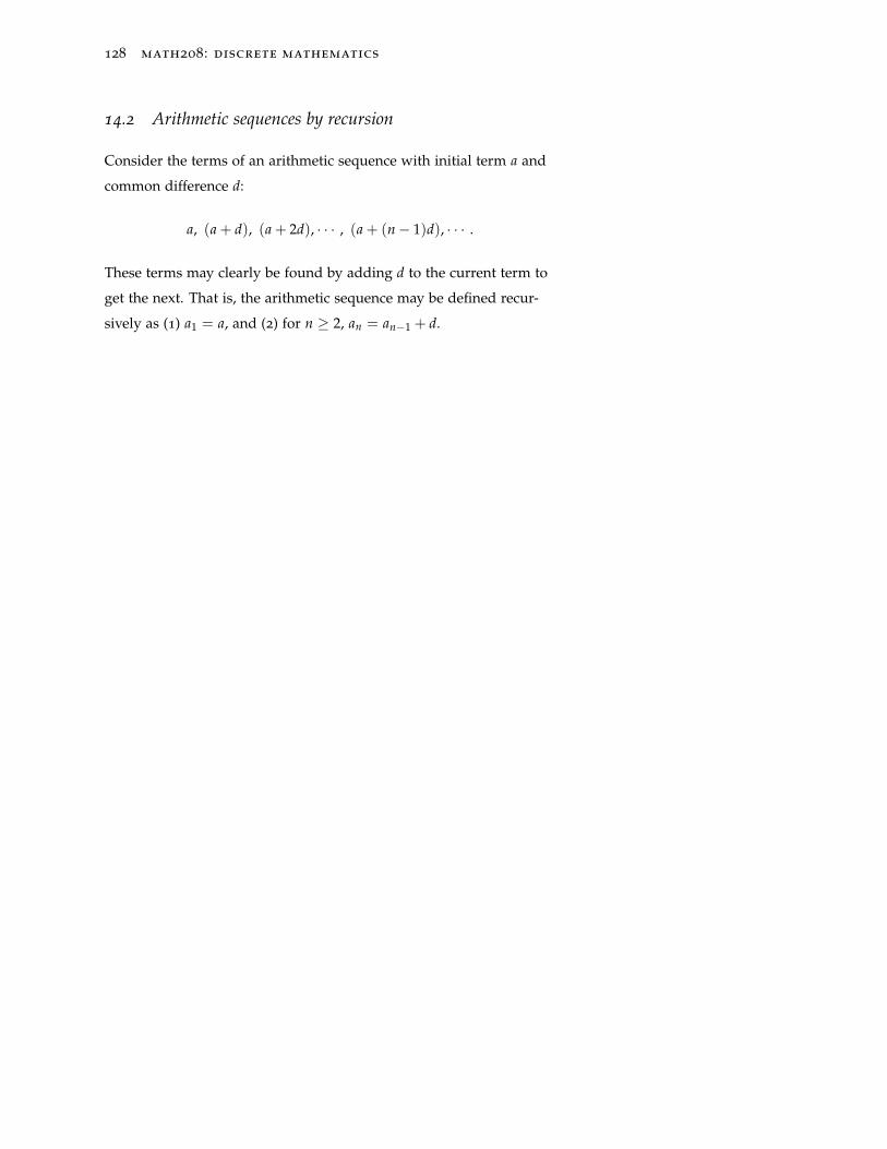
128 math208: discrete mathematics
14.2 Arithmetic sequences by recursion
Consider the terms of an arithmetic sequence with initial term a and
common difference d:
a, (a + d), (a + 2d), · · · , (a + (n− 1)d), · · · .
These terms may clearly be found by adding d to the current term to
get the next. That is, the arithmetic sequence may be defined recur-
sively as (1) a1 = a, and (2) for n ≥ 2, an = an−1 + d.
recursively defined sequences 129
14.3 Exercises
Exercise 14.1. List the first five terms of the sequence defined recursively by
a1 = 2, and, for n ≥ 2, an = a2n−1 − 1.
Exercise 14.2. List the first five terms of the sequence defined recursively by
a1 = 2, and, for n ≥ 2, an = 3an−1 + 2. Guess a closed form formula for Hint: This is a lot like example 14.2.
the sequence.
Exercise 14.3. List the first five terms of the sequence with initial terms
u0 = 2 and u1 = 5, and, for n ≥ 2, un = 5un−1 − 6un−2. Guess a closed Hint: The terms are simple combina-
tions of powers of 2 and powers of
3.form formula for the sequence.
Exercise 14.4. Let r be a fixed real number different from 0. For a positive
integer n, the symbol rn means the product of n r’s. For convenience, r0 is
defined to be 1. Give a recursive definition of rn analogous to the definition
of n! given in this chapter.
Exercise 14.5. Give a recursive definition of the geometric sequence with
initial term 3 and common ratio 2.
Exercise 14.6. Generalize exercise 5 to a generic geometric sequence with
initial term a and common ratio r.

15
Recursively Defined Sets
Two different ways of defining a set have been discussed. We can
describe a set by the roster method, listing all the elements that are to
be members of the set, or we can describe a set using set-builder no-
tation by giving a predicate that the elements of the set are to satisfy.
Here we consider defining sets in another natural way: recursion.
15.1 Recursive definitions of sets
Recursive definitions can also be used to build sets of objects. The
spirit is the same as for recursively defined sequences: give some ini-
tial conditions and a rule for building new objects from ones already
known.
Example 15.1. For instance, here is a way to recursively define the set
of positive even integers, E. First the initial condition: 2 ∈ E. Next the
recursive portion of the definition: If x ∈ E, then x + 2 ∈ E. Here is what
we can deduce using these two rules. First of course, we see 2 ∈ E since
that is the given initial condition. Next, since we know 2 ∈ E, the recursive
portion of the definition, with x being played by 2, says 2 + 2 ∈ E, so that
now we know 4 ∈ E. Since 4 ∈ E, the recursive portion of the definition,
with x now being played by 4, says 4 + 2 ∈ E, so that now we know 6 ∈ E.
Continuing in this way, it gets easy to believe that E really is the set of
positive even integers.
132 math208: discrete mathematics
Actually, there is a little more to do with example 15.1. The claim
is that E consists of exactly all the positive even integers. In other
words, we also need to make sure that no other things appear in E
besides the positive even integers. Could 312211 somehow have slith-
ered into the set E? To verify that such a thing does not happen, we
need one more fact about recursively defined sets. The only elements
that appear in a set defined recursively are those that make it on the
basis of either the initial condition or the recursive portion of the def-
inition. No elements of the set appear, as if by magic, from nowhere.
In this case, it is easy to see that no odd integers sneak into the
set. For if so, there would be a smallest odd integer in the set and the
only way it could be elected to the set is if the integer two less than it
were in the set. But that would mean a yet smaller odd integer would
be in the set, a contradiction. We won’t go into that sort of detail for
the following examples in general. We’ll just consider the topic at the
intuitive level only.
Example 15.2. Give a recursive definition of the set, S, of all nonnegative
integer powers of 2.
Initial condition: 1 ∈ S. Recursive rule: If x ∈ S, then 2x ∈ S.
Applying the initial condition and then the recursive rule repeatedly gives
the elements:
1 2 · 1 = 2 2 · 2 = 4 2 · 4 = 8 2 · 8 = 16
and so on, and that looks like the set of nonnegative powers of 2.
Example 15.3. A set, S, is defined recursively by
(1) (initial conditions) 1 ∈ S and 2 ∈ S, and
(2) (recursive rule) If x ∈ S, then x + 3 ∈ S. Describe the integers in S.
The plan is to use the initial conditions and the recursive rule to build
elements of S until we can guess a description of the integers in S. From the
initial conditions we know 1 ∈ S and 2 ∈ S. Applying the recursive rule
to each of those we get 4, 5 ∈ S, and using the recursive rule on those gives
7, 8 ∈ S, and so on.
So we get S = {1, 2, 4, 5, 7, 8, 10, 11, · · · } and it’s apparent that S
consists of of the positive integers that are not multiples of 3.
recursively defined sets 133
15.2 Sets of strings
Recursively defined sets appear in certain computer science courses
where they are used to describe sets of strings. To form a string, we
begin with an alphabet which is a set of symbols, traditionally de-
noted by Σ. For example Σ = {a, b, c} is an alphabet of three symbols,
and Σ = {!, @, #, $, %, &, X, 5} is an alphabet of eight symbols. A
string over the alphabet Σ is any finite sequence of symbols from
the alphabet. For example aaba is a string of length four over the
alphabet Σ = {a, b, c}, and !!5X$$5@@ is a length nine string over
Σ = {!, @, #, $, %, &, X, 5}. There is a special string over any alphabet
denoted by λ called the empty string. It contains no symbols, and
has length 0.
Example 15.4. A set, S, of strings over the alphabet Σ = {a, b} is given
recursively by (1) λ ∈ S, and (2) If x ∈ S, then axb ∈ S. Describe the
strings in S.
The notation axb means write down the string a followed by the string
x followed by the string b. So if x = aaba then axb = aaabab. Let’s
experiment with the recursive rule a bit, and then guess a description for the
strings in S. Starting with the initial condition we see λ ∈ S. Applying the
recursive rule to λ gives aλb = ab ∈ S. Applying the recursive rule to ab
gives aabb ∈ S, and applying the recursive rule to aabb shows aaabbb ∈ S.
It’s easy to guess the nature of the strings in S: Any finite string of a’s
followed by the same number of b’s.
Example 15.5. Give a recursive definition of the set S of strings over Σ =
{a, b, c} which do not contain adjacent a’s. For example ccabbbabba is
acceptable, but abcbaabaca is not.
For the initial conditions we will use (1) λ ∈ S, and a ∈ S. If we have a
string with no adjacent a’s, we can extend it by adding b or c to either end.
But we’ll need to be careful when adding more a’s. For the recursive rule we
will use (2) if x ∈ S, then bx, xb, cx, xc ∈ S and abx, xba, acx, xca ∈ S.
Notice how the string a had to be put into S in the initial conditions since
the recursive rule won’t allow us to form that string from λ.
Here is different answer to the same question. It’s a little harder
to dream up, but the rules are much cleaner. The idea is that if we
134 math208: discrete mathematics
take two strings with no adjacent a’s, we can put them together and
be sure to get a new string with no adjacent a’s provided we stick
either b or c between them. So, we can define the set recursively by
(1) λ ∈ S and a ∈ S, and (2) if x, y ∈ S, then xby, xcy ∈ S.
Example 15.6. Give a recursive definition of the set S of strings over Σ =
{a, b} which contain more a’s than b’s.
The idea is that we can build longer strings from smaller ones by (1)
sticking two such strings together, or (2) sticking two such strings together
along with a b before the first one, between the two strings, or after the last
one. That leads to the following recursive definition: (1) a ∈ S and (2) if
x, y ∈ S then xy, bxy, xby, xyb ∈ S. That looks a little weird since in the
recursive rule we added b, but since x and y each have more a’s than b’s, the
two together will have a least two more a’s than b’s, so it’s safe to add b in
the recursive rule.
Starting with the initial condition, and then applying the recursive rule
repeatedly, we form the following elements of S:
a, aa, baa, aba, aab, aaa, baaa, abaa, aaba, baaa, · · ·
Example 15.7. A set, S, of strings over the alphabet Σ = {a, b} is defined
recursively by the rules (1) a ∈ S, and (2) if x ∈ S, then xbx ∈ S. Describe
the strings in S.
Experimenting we find the following elements of S:
a, aba, abababa, abababababababa, · · ·
It looks like S is the set of strings beginning with a followed by a certain
number of ba’s. If we look at the number of ba’s in each string, we can see a
pattern: 0, 1, 3, 7, 15, 31, · · · , which we recognize as being the numbers that
are one less than the positive integer powers of 2 (1, 2, 4, 8, 16, 32, · · · ). So it
appears S is the set of strings which consisting of a followed by 2n − 1 pairs
ab for some integer n ≥ 0.
recursively defined sets 135
15.3 Exercises
Exercise 15.1. Give a recursive definition of the set of positive integers that
end with the digits 17.
Exercise 15.2. Give a recursive definition of the set of positive integers that
are not multiples of 4.
Exercise 15.3. A set S of ordered pairs of integers is defined recursively
by (1) (1, 1) ∈ S, and (2) if (m, n) ∈ S, then (m + 2, n) ∈ S, and
(m, n + 2) ∈ S, and (m + 1, n + 1) ∈ S. There is a simple description of the
ordered pairs in S. What is it?
Exercise 15.4. Describe the strings in the set S of strings over the alphabet
Σ = {a, b, c} defined recursively by (1) λ ∈ S and (2) if x ∈ S, then
axbc ∈ S.
Exercise 15.5. Describe the strings in the set S of strings over the alphabet
Σ = {a, b, c} defined recursively by (1) c ∈ S and (2) if x ∈ S then ax ∈ S
and bx ∈ S and xc ∈ S.
Exercise 15.6. A palindrome is a string that reads the same in both
directions. For example, aabaa is a palindrome of length five and babccbab
is a palindrome of length eight. Give a recursive definition of the set of
palindromes over the alphabet Σ = {a, b, c}.

16
Mathematical Induction
As mentioned earlier, to show that a proposition of the form
∀ x P(x) is true, it is necessary to check that P(c) is true for every
possible choice of c in the domain of discourse. If that domain is not
too big, it is feasible to check the truth of each P(c) one by one. For
instance, consider the proposition For every page in these notes, the
letter e appears at least once on the page. To express the proposition in
symbolic form we would let the domain of discourse be the set of
pages in these notes, and we would let the predicate E be has an oc-
currence of the letter e, so the proposition becomes ∀ p E(p). The truth
value of this proposition can be determined by the tedious but feasi-
ble task of checking every page of the notes for an e. If a single page
is found with no e’s, that page would constitute a counterexample to
the proposition, and the proposition would be false. Otherwise it is
true.
When the domain of discourse is a finite set, it is, in principle, al-
ways possible to check the truth of a proposition of the form ∀ x P(x)
by checking the members of the domain of discourse one by one. But
that option is no longer available if the domain of discourse is an in-
finite set since no matter how quickly the checks are made there is no
practical way to complete the checks in a finite amount of time. For
example, consider the proposition For every natural number n, n5 − n
ends with a 0.The truth of the proposition could be established by Here the domain of discourse is the set
N = { 0, 1, 2, 3, · · · }.
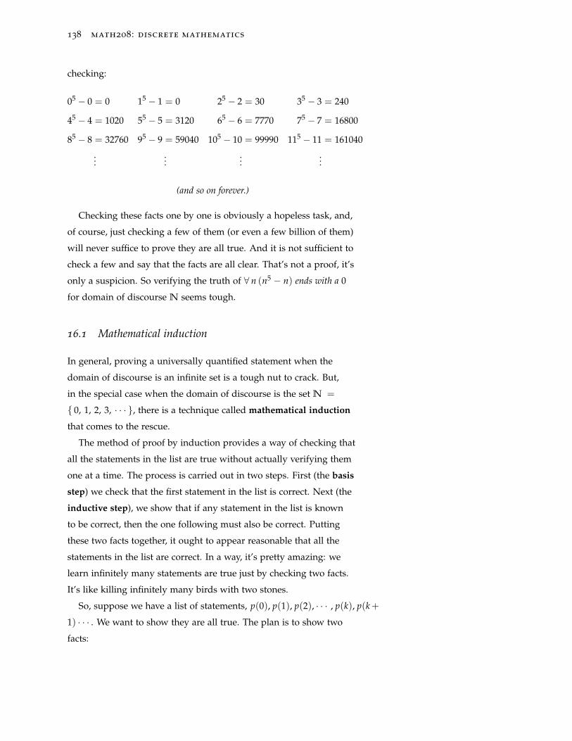
138 math208: discrete mathematics
checking:
05 − 0 = 0 15 − 1 = 0 25 − 2 = 30 35 − 3 = 240
45 − 4 = 1020 55 − 5 = 3120 65 − 6 = 7770 75 − 7 = 16800
85 − 8 = 32760 95 − 9 = 59040 105 − 10 = 99990 115 − 11 = 161040
......
......
(and so on forever.)
Checking these facts one by one is obviously a hopeless task, and,
of course, just checking a few of them (or even a few billion of them)
will never suffice to prove they are all true. And it is not sufficient to
check a few and say that the facts are all clear. That’s not a proof, it’s
only a suspicion. So verifying the truth of ∀ n (n5 − n) ends with a 0
for domain of discourse N seems tough.
16.1 Mathematical induction
In general, proving a universally quantified statement when the
domain of discourse is an infinite set is a tough nut to crack. But,
in the special case when the domain of discourse is the set N =
{ 0, 1, 2, 3, · · · }, there is a technique called mathematical induction
that comes to the rescue.
The method of proof by induction provides a way of checking that
all the statements in the list are true without actually verifying them
one at a time. The process is carried out in two steps. First (the basis
step) we check that the first statement in the list is correct. Next (the
inductive step), we show that if any statement in the list is known
to be correct, then the one following must also be correct. Putting
these two facts together, it ought to appear reasonable that all the
statements in the list are correct. In a way, it’s pretty amazing: we
learn infinitely many statements are true just by checking two facts.
It’s like killing infinitely many birds with two stones.
So, suppose we have a list of statements, p(0), p(1), p(2), · · · , p(k), p(k+
1) · · · . We want to show they are all true. The plan is to show two
facts:
mathematical induction 139
(1) p(0) is true, and
(2) for any n ∈N, p(n) −→ p(n + 1).
We then conclude all the statements in the list are true.
16.2 The principle of mathematical induction
The well ordering property of the positive integers provides the
justification for proof by induction. This property asserts that every
non-empty subset of the natural numbers contains a smallest number.
In fact, given any nonempty set of natural numbers, we can deter-
mine the smallest number in the set by the process of checking to see,
in turn, if 0 is in the set, and, if the answer is no, checking for 1, then
for 2, and so on. Since the set is nonempty, eventually the answer will
be yes, that number is in the set, and in that way, the smallest natural
number in the set will have been found. Now let’s look at the proof
that induction is a valid form of proof. The statement of the theorem
is a little more general than described above. Instead of beginning
with a statement p(0), we allow the list to begin with a statement
p(k) for some integer k (almost always, k = 0 or k = 1 in practice).
This does not have any effect of the concept of induction. In all cases,
we have a list of statements, and we show the first statement is true,
and then we show that if any statement is true, so is the next one.
The particular name for the starting point of the list doesn’t really
matter. It only matters that there is a starting point.
Theorem 16.1 (Principle of Mathematical Induction). Suppose we have
a list of statements p(k), p(k + 1), p(k + 2), · · · , p(n), p(n + 1) · · · .
(1) p(k) is true, and
(2) p(n) −→ p(n + 1) for every n ≥ k,
then all the statements in the list are true.
Proof. The proof will be by contradiction.
Suppose that 1 and 2 are true, but that it is not the case that p(n) is true
for all n ≥ k. Let S = {n|n ≥ k and p(n) is false}, so that S 6= ∅. Since
S is a non-empty set of integers ≥ k it has a least element, say t. So t is the
140 math208: discrete mathematics
smallest positive integer for which p(n) is false. In the ever colorful jargon
of mathematics, t is usually called the minimal criminal.
Since p(k) is true, k /∈ S. Therefore t > k. So t− 1 ≥ k. Since t is the
smallest integer ≥ k for which p is false, it must be that p(t − 1) is true.
Now, by part 2, we also know p(t− 1) → p(t) is true. So it must be that
p(t) is true, and that is a contradiction. ♣
16.3 Proofs by induction
Many people find proofs by induction a little bit black-magical at
first, but just keep the goals in mind (namely check [1] the first state-
ment in the list is true, and [2] that if any statement in the list is true,
so is the one that follows it) and the process won’t seem so confusing.
A handy way of viewing mathematical induction is to compare
proving the sequence p(k) ∧ p(k + 1) ∧ p(k + 2) ∧ ... ∧ p(m) ∧ ... to
knocking down a set of dominos set on edge and numbered consecu-
tively k, k + 1, ..... If we want to knock all of the dominos down, which
are numbered k and greater, then we must knock the kth domino
down, and ensure that the spacing of the dominos is such that ev-
ery domino will knock down its successor. If either the spacing is off
(∃m ≥ k with p(m) not implying p(m + 1)), or if we fail to knock
down the kth domino (we do not demonstrate that p(k) is true), then
there may be dominos left standing. When checking the inductive step,
p(n) → p(n + 1), the statement p(n), is
called the inductive hypothesis.To discover how to prove the inductive step most people start by
explicitly listing several of the first instances of the inductive hypoth-
esis p(n). Then, look for how to make, in a general way, an argument
from one, or more, instances to the next instance of the hypothesis.
Once an argument is discovered that allows us to advance from the
truth of previous one, or more, instances, that argument, in general
form, becomes the pattern for the proof on the inductive hypothesis.
Let’s examine an example.
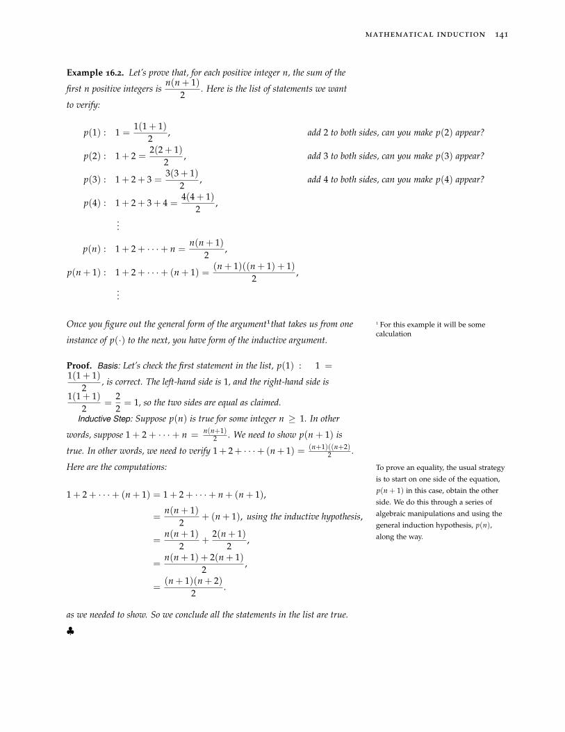
mathematical induction 141
Example 16.2. Let’s prove that, for each positive integer n, the sum of the
first n positive integers isn(n + 1)
2. Here is the list of statements we want
to verify:
p(1) : 1 =1(1 + 1)
2, add 2 to both sides, can you make p(2) appear?
p(2) : 1 + 2 =2(2 + 1)
2, add 3 to both sides, can you make p(3) appear?
p(3) : 1 + 2 + 3 =3(3 + 1)
2, add 4 to both sides, can you make p(4) appear?
p(4) : 1 + 2 + 3 + 4 =4(4 + 1)
2,
...
p(n) : 1 + 2 + · · ·+ n =n(n + 1)
2,
p(n + 1) : 1 + 2 + · · ·+ (n + 1) =(n + 1)((n + 1) + 1)
2,
...
Once you figure out the general form of the argument1that takes us from one 1 For this example it will be somecalculation
instance of p(·) to the next, you have form of the inductive argument.
Proof. Basis: Let’s check the first statement in the list, p(1) : 1 =1(1 + 1)
2, is correct. The left-hand side is 1, and the right-hand side is
1(1 + 1)2
=22= 1, so the two sides are equal as claimed.
Inductive Step: Suppose p(n) is true for some integer n ≥ 1. In other
words, suppose 1 + 2 + · · · + n = n(n+1)2 . We need to show p(n + 1) is
true. In other words, we need to verify 1+ 2+ · · ·+ (n+ 1) = (n+1)((n+2)2 .
Here are the computations: To prove an equality, the usual strategy
is to start on one side of the equation,
p(n + 1) in this case, obtain the other
side. We do this through a series of
algebraic manipulations and using the
general induction hypothesis, p(n),
along the way.
1 + 2 + · · ·+ (n + 1) = 1 + 2 + · · ·+ n + (n + 1),
=n(n + 1)
2+ (n + 1), using the inductive hypothesis,
=n(n + 1)
2+
2(n + 1)2
,
=n(n + 1) + 2(n + 1)
2,
=(n + 1)(n + 2)
2.
as we needed to show. So we conclude all the statements in the list are true.
♣
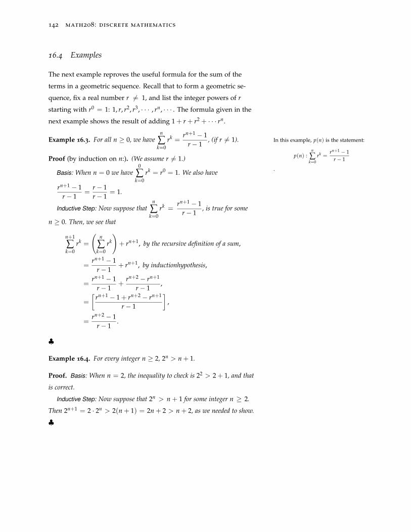
142 math208: discrete mathematics
16.4 Examples
The next example reproves the useful formula for the sum of the
terms in a geometric sequence. Recall that to form a geometric se-
quence, fix a real number r 6= 1, and list the integer powers of r
starting with r0 = 1: 1, r, r2, r3, · · · , rn, · · · . The formula given in the
next example shows the result of adding 1 + r + r2 + · · · rn.
Example 16.3. For all n ≥ 0, we haven
∑k=0
rk =rn+1 − 1
r− 1, (if r 6= 1). In this example, p(n) is the statement:
p(n) :n
∑k=0
rk =rn+1 − 1
r− 1
.
Proof (by induction on n:). (We assume r 6= 1.)
Basis: When n = 0 we have0
∑k=0
rk = r0 = 1. We also have
rn+1 − 1r− 1
=r− 1r− 1
= 1.
Inductive Step: Now suppose thatn
∑k=0
rk =rn+1 − 1
r− 1, is true for some
n ≥ 0. Then, we see that
n+1
∑k=0
rk =
(n
∑k=0
rk
)+ rn+1, by the recursive definition of a sum,
=rn+1 − 1
r− 1+ rn+1, by inductionhypothesis,
=rn+1 − 1
r− 1+
rn+2 − rn+1
r− 1,
=
[rn+1 − 1 + rn+2 − rn+1
r− 1
],
=rn+2 − 1
r− 1.
♣
Example 16.4. For every integer n ≥ 2, 2n > n + 1.
Proof. Basis: When n = 2, the inequality to check is 22 > 2 + 1, and that
is correct.
Inductive Step: Now suppose that 2n > n + 1 for some integer n ≥ 2.
Then 2n+1 = 2 · 2n > 2(n + 1) = 2n + 2 > n + 2, as we needed to show.
♣
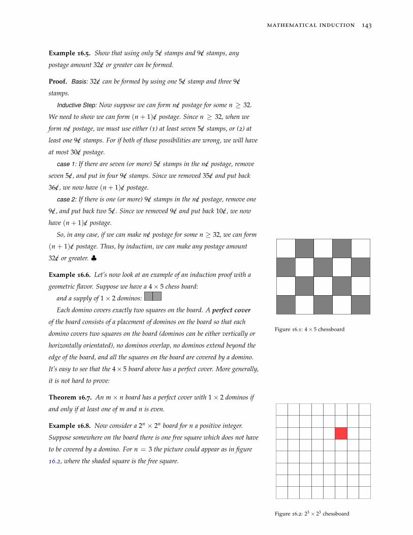
mathematical induction 143
Example 16.5. Show that using only 5c/ stamps and 9c/ stamps, any
postage amount 32c/ or greater can be formed.
Proof. Basis: 32c/ can be formed by using one 5c/ stamp and three 9c/
stamps.
Inductive Step: Now suppose we can form nc/ postage for some n ≥ 32.
We need to show we can form (n + 1)c/ postage. Since n ≥ 32, when we
form nc/ postage, we must use either (1) at least seven 5c/ stamps, or (2) at
least one 9c/ stamps. For if both of those possibilities are wrong, we will have
at most 30c/ postage.
case 1: If there are seven (or more) 5c/ stamps in the nc/ postage, remove
seven 5c/, and put in four 9c/ stamps. Since we removed 35c/ and put back
36c/, we now have (n + 1)c/ postage.
case 2: If there is one (or more) 9c/ stamps in the nc/ postage, remove one
9c/, and put back two 5c/. Since we removed 9c/ and put back 10c/, we now
have (n + 1)c/ postage.
So, in any case, if we can make nc/ postage for some n ≥ 32, we can form
(n + 1)c/ postage. Thus, by induction, we can make any postage amount
32c/ or greater. ♣
Example 16.6. Let’s now look at an example of an induction proof with a
geometric flavor. Suppose we have a 4× 5 chess board:
Figure 16.1: 4× 5 chessboard
and a supply of 1× 2 dominos:
Each domino covers exactly two squares on the board. A perfect cover
of the board consists of a placement of dominos on the board so that each
domino covers two squares on the board (dominos can be either vertically or
horizontally orientated), no dominos overlap, no dominos extend beyond the
edge of the board, and all the squares on the board are covered by a domino.
It’s easy to see that the 4× 5 board above has a perfect cover. More generally,
it is not hard to prove:
Theorem 16.7. An m× n board has a perfect cover with 1× 2 dominos if
and only if at least one of m and n is even.
Example 16.8. Now consider a 2n × 2n board for n a positive integer.
Suppose somewhere on the board there is one free square which does not have
to be covered by a domino. For n = 3 the picture could appear as in figure
16.2, where the shaded square is the free square.
Figure 16.2: 23 × 23 chessboard
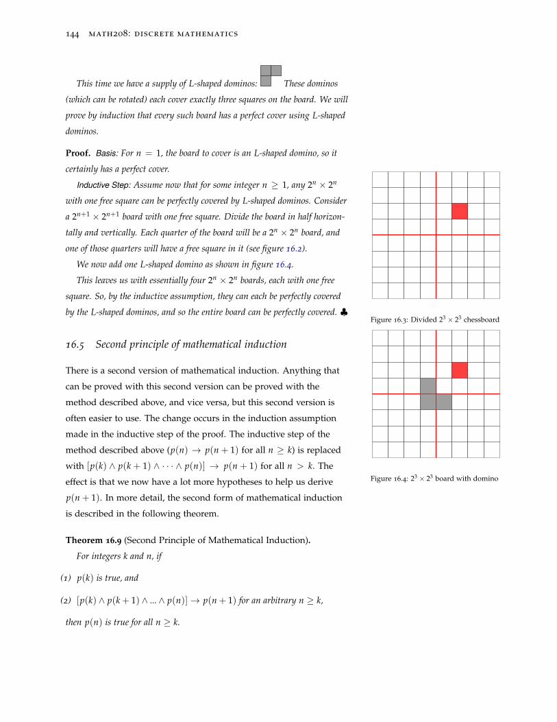
144 math208: discrete mathematics
This time we have a supply of L-shaped dominos: These dominos
(which can be rotated) each cover exactly three squares on the board. We will
prove by induction that every such board has a perfect cover using L-shaped
dominos.
Proof. Basis: For n = 1, the board to cover is an L-shaped domino, so it
certainly has a perfect cover.
Inductive Step: Assume now that for some integer n ≥ 1, any 2n × 2n
with one free square can be perfectly covered by L-shaped dominos. Consider
a 2n+1 × 2n+1 board with one free square. Divide the board in half horizon-
tally and vertically. Each quarter of the board will be a 2n × 2n board, and
one of those quarters will have a free square in it (see figure 16.2).
Figure 16.3: Divided 23 × 23 chessboard
We now add one L-shaped domino as shown in figure 16.4.
Figure 16.4: 23 × 23 board with domino
This leaves us with essentially four 2n × 2n boards, each with one free
square. So, by the inductive assumption, they can each be perfectly covered
by the L-shaped dominos, and so the entire board can be perfectly covered. ♣
16.5 Second principle of mathematical induction
There is a second version of mathematical induction. Anything that
can be proved with this second version can be proved with the
method described above, and vice versa, but this second version is
often easier to use. The change occurs in the induction assumption
made in the inductive step of the proof. The inductive step of the
method described above (p(n) → p(n + 1) for all n ≥ k) is replaced
with [p(k) ∧ p(k + 1) ∧ · · · ∧ p(n)] → p(n + 1) for all n > k. The
effect is that we now have a lot more hypotheses to help us derive
p(n + 1). In more detail, the second form of mathematical induction
is described in the following theorem.
Theorem 16.9 (Second Principle of Mathematical Induction).
For integers k and n, if
(1) p(k) is true, and
(2) [p(k) ∧ p(k + 1) ∧ ...∧ p(n)]→ p(n + 1) for an arbitrary n ≥ k,
then p(n) is true for all n ≥ k.
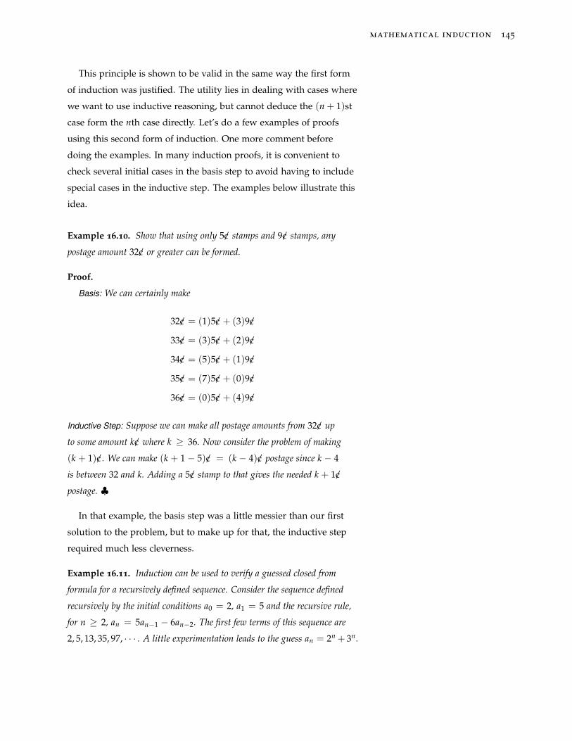
mathematical induction 145
This principle is shown to be valid in the same way the first form
of induction was justified. The utility lies in dealing with cases where
we want to use inductive reasoning, but cannot deduce the (n + 1)st
case form the nth case directly. Let’s do a few examples of proofs
using this second form of induction. One more comment before
doing the examples. In many induction proofs, it is convenient to
check several initial cases in the basis step to avoid having to include
special cases in the inductive step. The examples below illustrate this
idea.
Example 16.10. Show that using only 5c/ stamps and 9c/ stamps, any
postage amount 32c/ or greater can be formed.
Proof.
Basis: We can certainly make
32c/ = (1)5c/ + (3)9c/
33c/ = (3)5c/ + (2)9c/
34c/ = (5)5c/ + (1)9c/
35c/ = (7)5c/ + (0)9c/
36c/ = (0)5c/ + (4)9c/
Inductive Step: Suppose we can make all postage amounts from 32c/ up
to some amount kc/ where k ≥ 36. Now consider the problem of making
(k + 1)c/. We can make (k + 1 − 5)c/ = (k − 4)c/ postage since k − 4
is between 32 and k. Adding a 5c/ stamp to that gives the needed k + 1c/
postage. ♣
In that example, the basis step was a little messier than our first
solution to the problem, but to make up for that, the inductive step
required much less cleverness.
Example 16.11. Induction can be used to verify a guessed closed from
formula for a recursively defined sequence. Consider the sequence defined
recursively by the initial conditions a0 = 2, a1 = 5 and the recursive rule,
for n ≥ 2, an = 5an−1 − 6an−2. The first few terms of this sequence are
2, 5, 13, 35, 97, · · · . A little experimentation leads to the guess an = 2n + 3n.
146 math208: discrete mathematics
Let’s verify that guess using induction. For the basis of the induction we
check our guess gives the correct value of an for n = 0 and n = 1. That’s
easy. For the inductive step, let’s suppose our guess is correct up to n where
n ≥ 2. Then, we have
an+1 = 5an − 6an−1,
= 5(2n + 3n)− 6(2n−1 + 3n−1),
= (5 · 2− 6)2n−1 − (6− 5 · 3)3n−1,
= 4 · 2n−1 − (−9) · 3n−1,
= 2n+1 + 3n+1, as we needed to show.
Example 16.12. In the game of Nim, two players are presented with a pile
of matches. The players take turns removing one, two, or three matches at
a time. The player forced to take the last match is the loser. For example, if
the pile initially contains 8 matches, then first player can, with correct play,
be sure to win. Here’s how: player 1: take 3 matches leaving 5; player 2’s
options will leave 4, 3, or 2 matches, and so player 1 can reduce the pile to
1 match on her turn, thus winning the game. Notice that if player 1 takes
only 1 or 2 matches on her first turn, she is bound to lose to good play since
player 2 can then reduce the pile to 5 matches.
Let’s prove that if the number of matches in the pile is 1 more than a
multiple of 4, the second player can force a win; otherwise, the first player
can force a win.
Proof. For the basis, we note that obviously the second player wins if there
is 1 match in the pile, and for 2, 3, or 4 matches the first player wins by
taking 1, 2, or 3 matches in each case, leaving 1 match.
For the inductive step, suppose the statement we are to prove is correct
for the number of matches anywhere from 1 up to k for some k ≥ 4. Now
consider a pile of k + 1 matches.
case 1: If k + 1 is 1 more than a multiple of 4, then when player 1 takes
her matches, the pile will not contain 1 more than a multiple of 4 matches,
and so the next player can force a win by the inductive assumption. So
player 2 can force a win.
case 2: If k + 1 is not 1 more than a multiple of 4, then player 1 can
select matches to make it 1 more than a multiple of 4, and so the next player
mathematical induction 147
is bound to lose (with best play) by the inductive assumption. So player 1
can force a win. ♣
So, to win at Nim, when it is your turn, make sure you leave 1
more than a multiple of 4 matches in the pile (which is easy to do
unless your opponent knows the secret as well, in which case you can
just count the number of matches in the pile to see who will win, and
skip playing the game altogether!).
148 math208: discrete mathematics
16.6 Exercises
Exercise 16.1. Prove: For every integer n ≥ 1,
1 · 2 + 2 · 3 + 3 · 4 + · · ·+ n(n + 1) =n(n + 1)(n + 2)
3
Exercise 16.2. Prove: For every integer n ≥ 1,
11 · 2 +
12 · 3 +
13 · 4 + · · ·+ 1
n(n + 1)=
nn + 1
.
Exercise 16.3. Prove: For every integer n ≥ 1,
1 · 21 + 2 · 22 + 3 · 23 + ... + n · 2n = (n− 1)2n+1 + 2
Exercise 16.4. Show that using only 3c/ stamps and 5c/ stamps, any postage
amount 8c/ or greater can be formed. Do this twice, using both styles of
induction.
Exercise 16.5. Prove: For every integer n > 4, we have 2n > n2.
Exercise 16.6. Prove: For every integer n ≥ 1, the number n5 − n is a
multiple of 5.
Exercise 16.7. A pizza is cut into pieces (maybe some pretty oddly shaped)
by making some integer n ≥ 0 number of straight line cuts. Prove: The
maximum number of pieces isn2 + n + 2
2.
Exercise 16.8. A sequence is defined recursively by a0 = 0, and, for n ≥ 1,
an = 5an−1 + 1. Use induction to prove the closed form formula for an is
an =5n − 1
4.
Exercise 16.9. A sequence is defined recursively by a0 = 1, a1 = 4, and for
n ≥ 2, an = 5an−1 − 6an−2. Use induction to prove that the closed form
formula for an is an = 2 · 3n − 2n, n ≥ 0.
17
Algorithms
An algorithm is a recipe to solve a problem. For example, here is
an algorithm that solves the problem of finding the distance traveled
by a car given the time it has traveled, t, and its average speed, s:
multiply t and s.
17.1 Properties of an algorithm
Over time, the requirements of what exactly constitutes an algorithm
have matured. A really precise definition would be filled with all
sorts of technical jargon, but the ideas are commonsensible enough
that an informal description will suffice for our purposes. So, sup-
pose we have in mind a certain class of problems (such as determine
the distance traveled given time traveled and average speed). The
properties of an algorithm to solve examples of that class of problems
are:
(1) Input: The algorithm is provided with data.
(2) Output: The algorithm produces a solution.
(3) Definiteness: The instructions that make up the algorithm are
precisely described. They are not open to interpretation.
(4) Finiteness: The output is produced in a finite number of steps.
(5) Generality: The algorithm produces correct output for any set of
input values.
150 math208: discrete mathematics
The algorithm for finding distance traveled given time traveled
and average speed obviously meets all five requirements of an algo-
rithm. Notice that, in this example, we have assumed the user of the
algorithm understands what it means to multiply two numbers. If we
cannot make that assumption, then we would need to add a number
of additional steps to the algorithm to solve the problem of multiply-
ing two numbers together. Of course, that would make the algorithm
significantly longer. When describing algorithms, we’ll assume the
user knows the usual algorithms for solving common problems such
as addition, subtraction, multiplication, and division of numbers, and
knows how to determine if one number is larger than another, and so
on.
17.2 Non-algorithms
Just as important as an example of what an algorithm is, is an exam-
ple of what is not an algorithm. For example, we might describe the
method by which most people look up a number in a phone book.
You open the book and look to see if the listing you’re looking for is
on that page or not. If it is you find the number using the fact that
the listings are alphabetized and you’re done. If the number you’re
looking for is not on the page, you use the fact that the listings are al-
phabetized to either flip back several pages, or forward several pages.
This page is checked to see if the listing is on it. If it is not we repeat
the process. One problem in this case is that this description is not
definite. The phrase flip back several pages is too vague, it violates the
definiteness requirement. Another problem is that someone could
flip back and forth between two pages and never find the number,
and so violate the finiteness requirement. So this method is not an
algorithm.
17.3 Linear search algorithm
Continuing the example from section 17.2 of looking up a phone
number, one algorithm for completing this is to look at the first entry
in the book. If it’s the number you’re looking for you’re done. Else
algorithms 151
move to the next entry. It’s either the number you’re looking for or
you move to the next entry. This is an example of a linear search
algorithm. It’s not too bad for finding Adam Aaronson’s number if
he is in the book, but it is terrible if you’re trying to reach Zebulon
Zyzniewski.
17.4 Binary search algorithm
Another algorithm to complete that task of finding a phone number
is the binary search algorithm. We open the phone book to the mid-
dle entry. If it’s the number we’re looking for, we’re done. Else we
know the number is listed in the first half of the book, or the last half
of the book since the entries are alphabetized. We then pick the mid-
dle entry of the appropriate half, and repeat the halving process on
that half, until eventually the name is located. There are a few details
to fix up to make this a genuine algorithm. For example, what is the
middle entry if there are an even number of items listed? Also, what
happens if the name we are looking for isn’t in the phone book? But
it is clear with a little effort we can add a few lines to the instructions
to make this process into an algorithm.
17.5 Presenting algorithms
It is traditional to present algorithms in a pseudocode form similar
to a program for a computer. For instance, the linear search name
lookup algorithm given above could be written in pseudocode form,
as shown in Algorithm 17.1 on page 152. Another version using a for
loop is displayed in Agorithm 17.2.
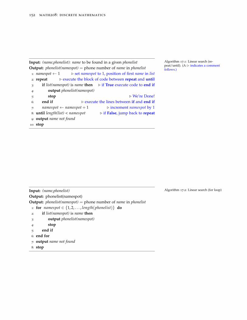
152 math208: discrete mathematics
Input: (name,phonelist): name to be found in a given phonelistOutput: phonelist(namespot) = phone number of name in phonelist
1: namespot← 1 . set namespot to 1, position of first name in list2: repeat . execute the block of code between repeat and until3: if list(namespot) is name then . if True execute code to end if4: output phonelist(namespot)5: stop . We’re Done!6: end if . execute the lines between if and end if7: namespot← namespot + 1 . increment namespot by 18: until length(list) < namespot . if False, jump back to repeat9: output name not found
10: stop
Algorithm 17.1: Linear search (re-peat/until). (A B indicates a commentfollows.)
Input: (name,phonelist)Output: phonelist(namespot)Output: phonelist(namespot) = phone number of name in phonelist
1: for namespot ∈ {1, 2, . . . , length(phonelist)} do2: if list(namespot) is name then3: output phonelist(namespot)4: stop5: end if6: end for7: output name not found8: stop
Algorithm 17.2: Linear search (for loop)
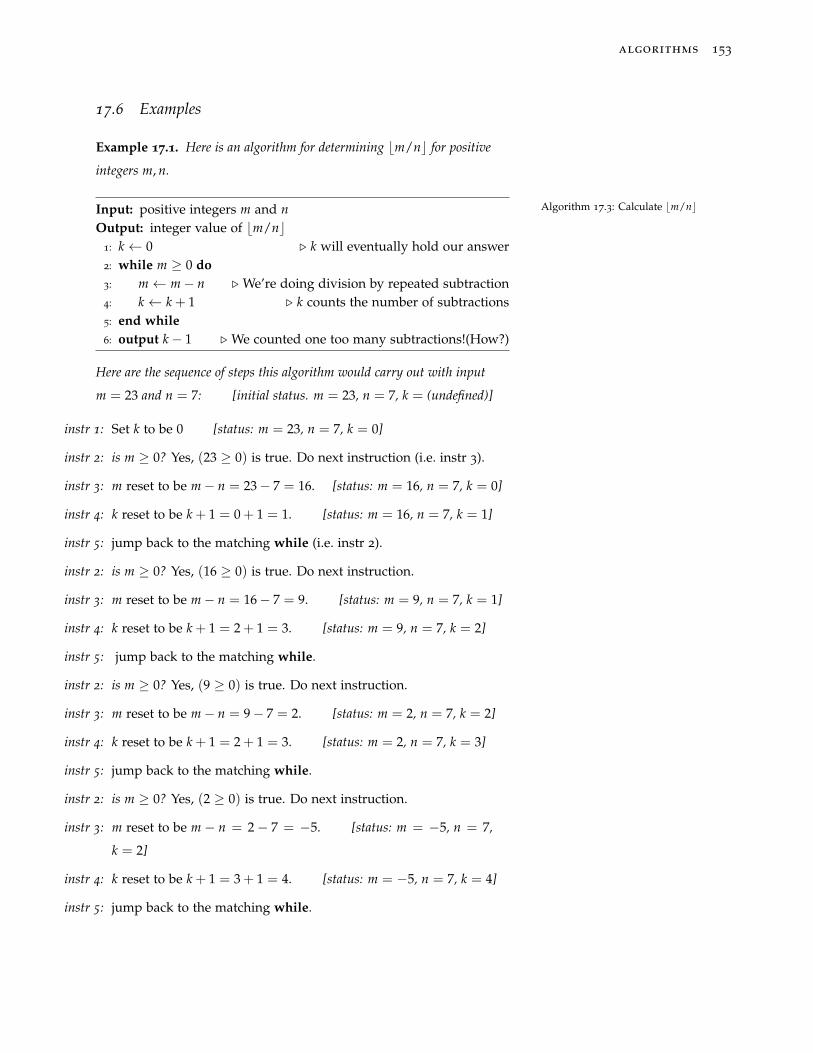
algorithms 153
17.6 Examples
Example 17.1. Here is an algorithm for determining bm/nc for positive
integers m, n.
Input: positive integers m and nOutput: integer value of bm/nc
1: k← 0 . k will eventually hold our answer2: while m ≥ 0 do3: m← m− n . We’re doing division by repeated subtraction4: k← k + 1 . k counts the number of subtractions5: end while6: output k− 1 . We counted one too many subtractions!(How?)
Algorithm 17.3: Calculate bm/nc
Here are the sequence of steps this algorithm would carry out with input
m = 23 and n = 7: [initial status. m = 23, n = 7, k = (undefined)]
instr 1: Set k to be 0 [status: m = 23, n = 7, k = 0]
instr 2: is m ≥ 0? Yes, (23 ≥ 0) is true. Do next instruction (i.e. instr 3).
instr 3: m reset to be m− n = 23− 7 = 16. [status: m = 16, n = 7, k = 0]
instr 4: k reset to be k + 1 = 0 + 1 = 1. [status: m = 16, n = 7, k = 1]
instr 5: jump back to the matching while (i.e. instr 2).
instr 2: is m ≥ 0? Yes, (16 ≥ 0) is true. Do next instruction.
instr 3: m reset to be m− n = 16− 7 = 9. [status: m = 9, n = 7, k = 1]
instr 4: k reset to be k + 1 = 2 + 1 = 3. [status: m = 9, n = 7, k = 2]
instr 5: jump back to the matching while.
instr 2: is m ≥ 0? Yes, (9 ≥ 0) is true. Do next instruction.
instr 3: m reset to be m− n = 9− 7 = 2. [status: m = 2, n = 7, k = 2]
instr 4: k reset to be k + 1 = 2 + 1 = 3. [status: m = 2, n = 7, k = 3]
instr 5: jump back to the matching while.
instr 2: is m ≥ 0? Yes, (2 ≥ 0) is true. Do next instruction.
instr 3: m reset to be m − n = 2− 7 = −5. [status: m = −5, n = 7,
k = 2]
instr 4: k reset to be k + 1 = 3 + 1 = 4. [status: m = −5, n = 7, k = 4]
instr 5: jump back to the matching while.
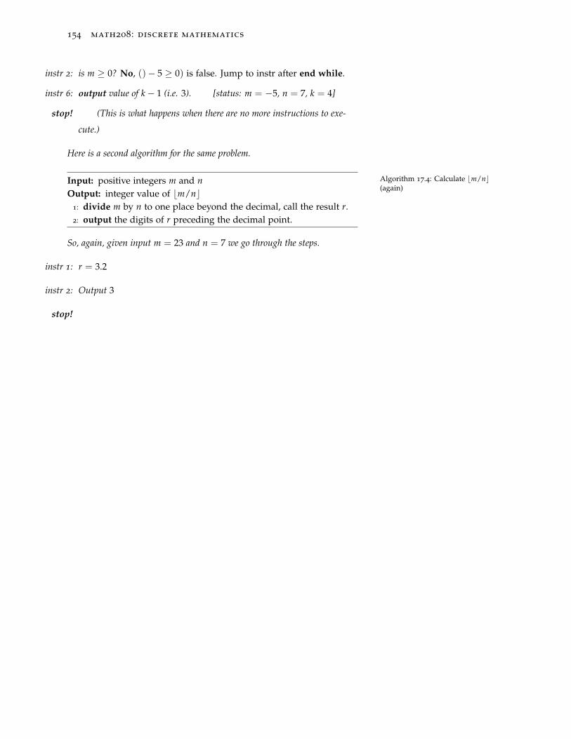
154 math208: discrete mathematics
instr 2: is m ≥ 0? No, ()− 5 ≥ 0) is false. Jump to instr after end while.
instr 6: output value of k− 1 (i.e. 3). [status: m = −5, n = 7, k = 4]
stop! (This is what happens when there are no more instructions to exe-
cute.)
Here is a second algorithm for the same problem.
Input: positive integers m and nOutput: integer value of bm/nc
1: divide m by n to one place beyond the decimal, call the result r.2: output the digits of r preceding the decimal point.
Algorithm 17.4: Calculate bm/nc(again)
So, again, given input m = 23 and n = 7 we go through the steps.
instr 1: r = 3.2
instr 2: Output 3
stop!

algorithms 155
Example 17.2. An algorithm to make $n change using $10, $5, and $1
bills.
Input: positive integers m and nOutput: integer value of bm/nc
1: while n ≥ 10 do2: output $103: n← n− 104: end while5: while n ≥ 5 do6: output $57: n← n− 58: end while9: while n ≥ 1 do
10: output $111: n← n− 112: end while
Algorithm 17.5: Make change
For an input of 27, the output would be $10, $10, $5, $1, $1.
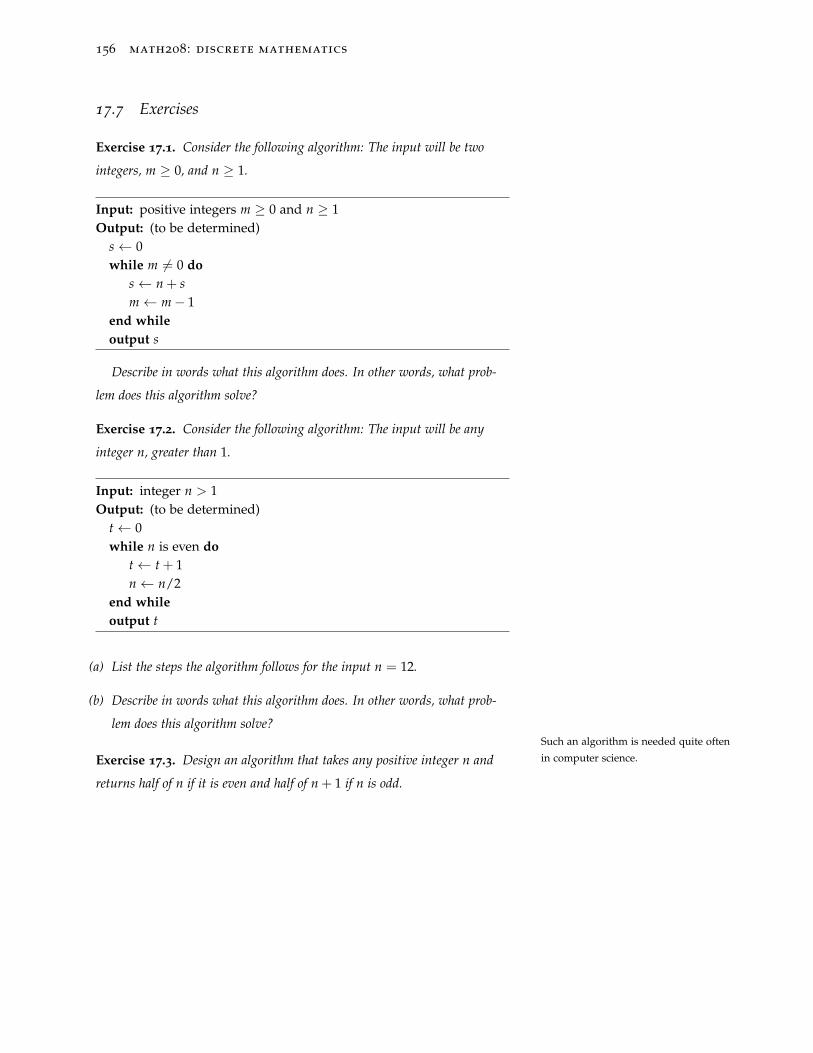
156 math208: discrete mathematics
17.7 Exercises
Exercise 17.1. Consider the following algorithm: The input will be two
integers, m ≥ 0, and n ≥ 1.
Input: positive integers m ≥ 0 and n ≥ 1Output: (to be determined)
s← 0while m 6= 0 do
s← n + sm← m− 1
end whileoutput s
Describe in words what this algorithm does. In other words, what prob-
lem does this algorithm solve?
Exercise 17.2. Consider the following algorithm: The input will be any
integer n, greater than 1.
Input: integer n > 1Output: (to be determined)
t← 0while n is even do
t← t + 1n← n/2
end whileoutput t
(a) List the steps the algorithm follows for the input n = 12.
(b) Describe in words what this algorithm does. In other words, what prob-
lem does this algorithm solve?Such an algorithm is needed quite often
in computer science.Exercise 17.3. Design an algorithm that takes any positive integer n and
returns half of n if it is even and half of n + 1 if n is odd.
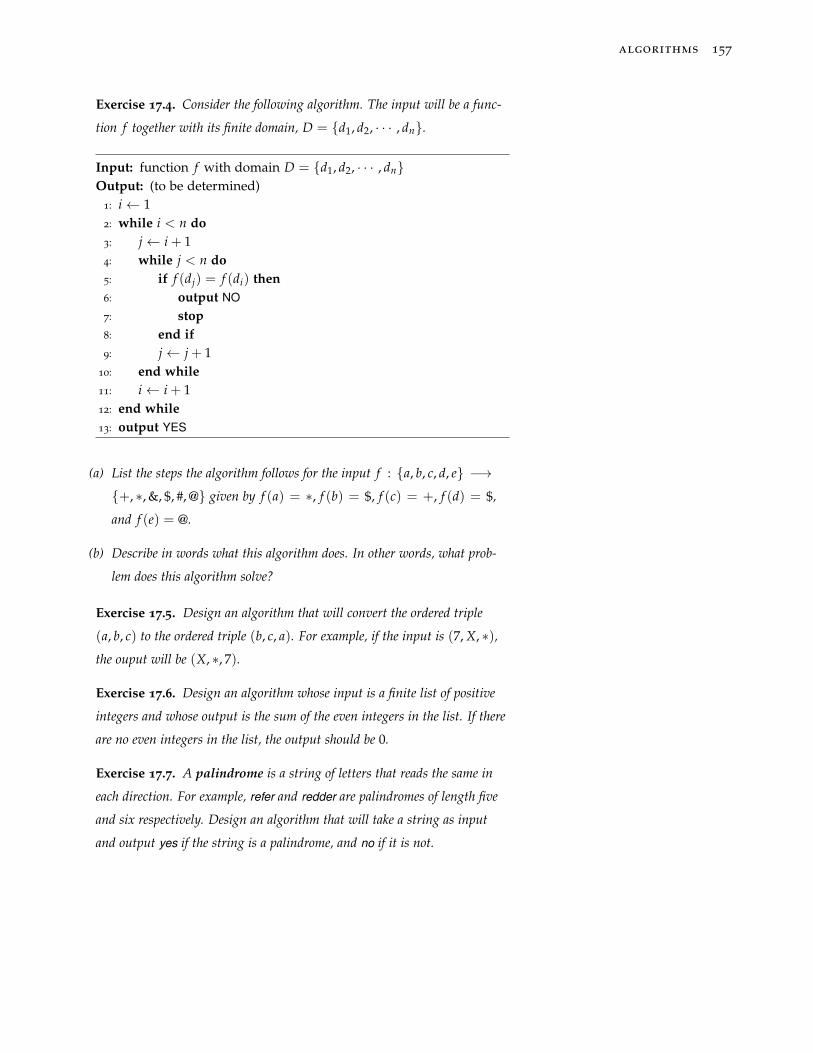
algorithms 157
Exercise 17.4. Consider the following algorithm. The input will be a func-
tion f together with its finite domain, D = {d1, d2, · · · , dn}.
Input: function f with domain D = {d1, d2, · · · , dn}Output: (to be determined)
1: i← 12: while i < n do3: j← i + 14: while j < n do5: if f (dj) = f (di) then6: output NO
7: stop8: end if9: j← j + 1
10: end while11: i← i + 112: end while13: output YES
(a) List the steps the algorithm follows for the input f : {a, b, c, d, e} −→{+, ∗, &, $, #, @} given by f (a) = ∗, f (b) = $, f (c) = +, f (d) = $,
and f (e) = @.
(b) Describe in words what this algorithm does. In other words, what prob-
lem does this algorithm solve?
Exercise 17.5. Design an algorithm that will convert the ordered triple
(a, b, c) to the ordered triple (b, c, a). For example, if the input is (7, X, ∗),the ouput will be (X, ∗, 7).
Exercise 17.6. Design an algorithm whose input is a finite list of positive
integers and whose output is the sum of the even integers in the list. If there
are no even integers in the list, the output should be 0.
Exercise 17.7. A palindrome is a string of letters that reads the same in
each direction. For example, refer and redder are palindromes of length five
and six respectively. Design an algorithm that will take a string as input
and output yes if the string is a palindrome, and no if it is not.

18
Algorithm Efficiency
There are many different algorithms for solving any partic-
ular class of problems. In the last chapter, we considered two algo-
rithms for solving the problem of looking up a phone number given
a person’s name.
Algorithm L: Look at the first entry in the book. If it’s the number
you’re looking for you’re done. Else move to the next entry. It’s either
the number you’re looking for or you move to the next entry, and so
on. (The linear search algorithm)
Algorithm B: The second algorithm took advantage of the arrange-
ment of a phone book in alphabetical order. We open the phone book
to the middle entry. If it’s the number we’re looking for, we’re done.
Otherwise we know the number is listed in the first half of the book,
or the last half of the book. We then pick the middle entry of the ap-
propriate half, and repeat the process. After a number of repetitions,
we will either be at the name we want, or learn the name isn’t in the
book. (The binary search algorithm)
The question arises, which algorithm is better? The question is
pretty vague. Let’s assume that better means uses fewer steps. Now if
there are only one or two names in the phone book, it doesn’t matter
which algorithm we use, the look-up always takes one or two steps.
But what if the phone book contains 10000 names? In this case, it is
hard to say which algorithm is better: looking up Adam Aaronson
will likely only take one step by the linear search algorithm, but
binary search will take 14 steps or so. But for Zebulon Zyzniewski,
160 math208: discrete mathematics
the linear search will take 10000 steps, while the binary search will
again take about 14 steps.
18.1 Comparing algorithms
There are two lessons to be learned from those last examples:
(1) Small cases of the problem can be misleading when judging the
quality of an algorithm, and
(2) It’s unlikely that one algorithm will always be more efficient than
another.
The common approach to compare the efficiency of two algorithms
takes those two lessons into account by agreeing to the following
protocol:
(1) only compare the algorithms when the size, n, of the problem it is
applied to is huge. In the phone book example, don’t worry about
phone books of 100 names or even 10000 names. Worry instead
about phone books with n names where n gets arbitrarily large.
(2) to compare two algorithms, first, for each algorithm, find the max-
imum number of steps ever needed when applied to a problem of
size n. For a phone book of size n the linear search algorithm will
require n steps in the worst possible case of the name not being
in the book. On the other hand, the halving process of the binary
search algorithm means that it will never take more than about
log2 n steps to locate a name (or discover the name is missing)
in the phone book. This information is expressed compactly by
saying the linear search algorithm has worst case scenario effi-
ciency wL(n) = n while the binary search algorithm has worst case
scenario efficiency wB(n) = log2 n.
(3) we declare that algorithm #1 is more efficient than algorithm
#2 provided, for all problems of huge sizes n, w1(n) < w2(n),
where w1 and w2 are the worst case scenario efficiencies for each
algorithm.
algorithm efficiency 161
Notice that for huge n, wB(n) < wL(n). In fact, there is no real
contest. For example, when n = 1048576 = 220, we get wB(n) = 20
while wL(n) = 1048576, and things only get better for wB as n gets
larger.
In summary, to compare two algorithms designed to solve the
same class of problems we:
(1) Determine a number n that indicates the size of the a problem. For
example, if the algorithm manipulates a list of numbers, n could
be the length of the list. If the algorithm is designed to raise a
number to a power, the size could be the power n.
(2) Decide what will be called a step when applying the algorithms.
In the phone book example, we took a step to mean a comparison.
When raising a number to a power, a step might consist of per-
forming a multiplication. A step is usually taken to be the most
time consuming action in the algorithm, and other actions are ig-
nored. Also, when determining the function, w don’t get hung up
worrying about miniscule details. Don’t spend time trying to de-
termine if w(n) = 2n + 7 or w(n) = 2n + 67. For huge values of n,
the +7 and +67 become unimportant. In such a case, w(n) = 2n
has all the interesting information. Don’t sweat the small stuff.
(3) Determine the worst case scenario functions for the two algo-
rithms, and compare them. The smaller of the two (assuming they
are not essentially the same) is declared the more efficient algo-
rithm.
Example 18.1. Let’s do a worst case scenario computation for the following
algorithm designed to determine the largest number in a list of n numbers.
It would be natural to use the number of items in the list, n, to represent
the size of a problem. And let’s use the comparisons as steps. We are going
to make two comparisons each for each of the items in the list in every case
(every case is a worst case for this algorithm!). So we give this algorithm an
efficiency w(n) = 2n. Notice that we actually only need comparisons for the
last n− 1 items in the list, and the exact number of times the comparisons
in instructions (3) and (4) are carried out might take a few minutes to figure
out. But it’s clear that both are carried out about n times, and since we are
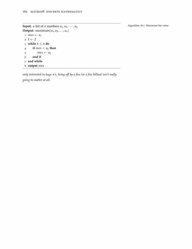
162 math208: discrete mathematics
Input: a list of n numbers a1, a2, · · · , an
Output: maximum(a1, a2, . . . , an)
1: max ← a1
2: k← 23: while k ≤ n do4: if max < ak then5: max ← ak
6: end if7: end while8: output max
Algorithm 18.1: Maximum list value
only interested in huge n’s, being off by a few (or a few billion) isn’t really
going to matter at all.
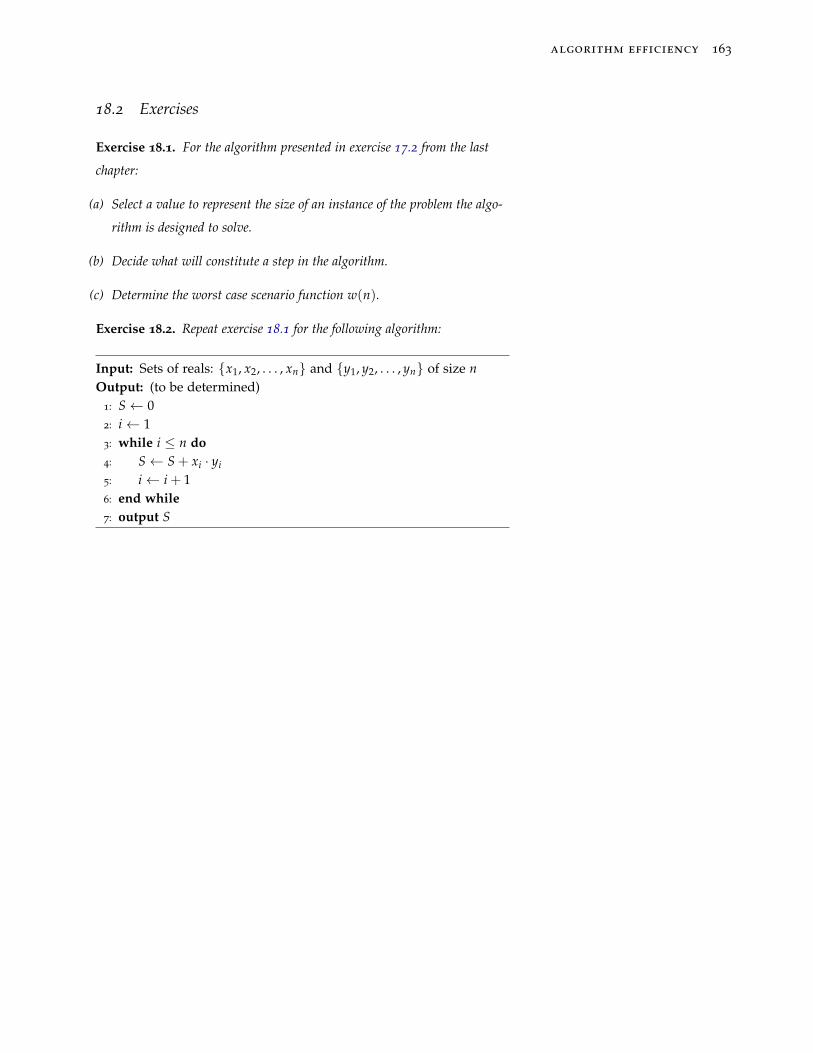
algorithm efficiency 163
18.2 Exercises
Exercise 18.1. For the algorithm presented in exercise 17.2 from the last
chapter:
(a) Select a value to represent the size of an instance of the problem the algo-
rithm is designed to solve.
(b) Decide what will constitute a step in the algorithm.
(c) Determine the worst case scenario function w(n).
Exercise 18.2. Repeat exercise 18.1 for the following algorithm:
Input: Sets of reals: {x1, x2, . . . , xn} and {y1, y2, . . . , yn} of size nOutput: (to be determined)
1: S← 02: i← 13: while i ≤ n do4: S← S + xi · yi
5: i← i + 16: end while7: output S

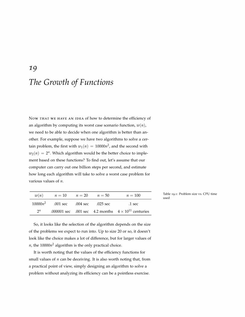
19
The Growth of Functions
Now that we have an idea of how to determine the efficiency of
an algorithm by computing its worst case scenario function, w(n),
we need to be able to decide when one algorithm is better than an-
other. For example, suppose we have two algorithms to solve a cer-
tain problem, the first with w1(n) = 10000n2, and the second with
w2(n) = 2n. Which algorithm would be the better choice to imple-
ment based on these functions? To find out, let’s assume that our
computer can carry out one billion steps per second, and estimate
how long each algorithm will take to solve a worst case problem for
various values of n.
w(n) n = 10 n = 20 n = 50 n = 100
10000n2 .001 sec .004 sec .025 sec .1 sec
2n .000001 sec .001 sec 4.2 months 4× 10¹¹ centuries
Table 19.1: Problem size vs. CPU timeused
So, it looks like the selection of the algorithm depends on the size
of the problems we expect to run into. Up to size 20 or so, it doesn’t
look like the choice makes a lot of difference, but for larger values of
n, the 10000n2 algorithm is the only practical choice.
It is worth noting that the values of the efficiency functions for
small values of n can be deceiving. It is also worth noting that, from
a practical point of view, simply designing an algorithm to solve a
problem without analyzing its efficiency can be a pointless exercise.
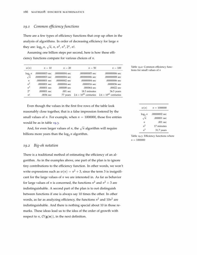
166 math208: discrete mathematics
19.1 Common efficiency functions
There are a few types of efficiency functions that crop up often in the
analysis of algorithms. In order of decreasing efficiency for large n
they are: log2 n,√
n, n, n2, n3, 2n, n!.
Assuming one billion steps per second, here is how these effi-
ciency functions compare for various choices of n.
w(n) n = 10 n = 20 n = 50 n = 100
log2 n .000000003 sec .000000004 sec .000000005 sec .000000006 sec√n .000000003 sec .000000004 sec .000000006 sec .000000008 sec
n .00000001 sec .00000002 sec .00000004 sec .00000006 secn2 .0000001 sec .0000004 sec .0000016 sec .0000036 secn3 .000001 sec .000008 sec .000064 sec .00022 sec2n .000001 sec .001 sec 18.3 minutes 36.5 yearsn! .0036 sec 77 years 2.6× 1029 centuries 2.6× 1063 centuries
Table 19.2: Common efficiency func-tions for small values of n
Even though the values in the first five rows of the table look
reasonably close together, that is a false impression fostered by the
small values of n. For example, when n = 1000000, those five entries
would be as in table 19.3.
w(n) n = 1000000
log2 n .00000002 sec√n .000001 sec
n .001 sec
n2 17 minutes
n3 31.7 years
Table 19.3: Efficiency functions where
n = 1000000
And, for even larger values of n, the√
n algorithm will require
billions more years than the log2 n algorithm.
19.2 Big-oh notation
There is a traditional method of estimating the efficiency of an al-
gorithm. As in the examples above, one part of the plan is to ignore
tiny contributions to the efficiency function. In other words, we won’t
write expressions such as w(n) = n2 + 3, since the term 3 is insignifi-
cant for the large values of n we are interested in. As far as behavior
for large values of n is concerned, the functions n2 and n2 + 3 are
indistinguishable. A second part of the plan is to not distinguish
between functions if one is always say 10 times the other. In other
words, as far as analyzing efficiency, the functions n2 and 10n2 are
indistinguishable. And there is nothing special about 10 in those re-
marks. These ideas lead us to the idea of the order of growth with
respect to n, O(g(n)), in the next definition.
the growth of functions 167
Definition 19.1. The function w(n) is O(g(n))provided there is a The symbol O(g(n)) is read in english
as big-oh of g(n).number k > 0 such that w(n) ≤ kg(n) for all n (or at least for all large
values of n).
As an example, n3 + 2n2 + 10n + 4 ≤ (1 + 2 + 10 + 4)n3 = 17n3
is O(n3). So if we have an algorithm with efficiency function w(n) =
n3 + 2n2 + 10n + 4, we can suppress all the unimportant details,
and simply say the efficiency is O(n3). In this example, it is also true
that w(n) is O(n4), but that is less precise information. On the other
hand, saying w(n) is O(n2) is certainly false. To indicate that we have
the best possible big-oh estimate allowed by our analysis, we would
say w(n) is at best O(n3). O(g(n)) actually represents the set
of functions dominated by g(n). So,
it would be proper to write w(n) =
n3 + 2n2 + 10n + 4 ∈ O(n3). Moreover,
we could write O(n2) ⊂ O(n3) since
the functions dominated by n2 are
among those dominated by n3.
Loosely speaking, finding the O estimate for a function selects the
most influential, or dominant, term (for large values of the variable)
in the function, and suppresses any constant factor for that term.
19.3 Examples
In each example, we find a big-oh estimate for the given expression.
Example 19.2. We have that n4 − 3n3 + 2n2 − 6n + 14 is O(n4), since for
large n the first term dominates the others.
Example 19.3. For large n, we have the inequalities:
(n3 log2 n + n2 − 3)(n2 + 2n + 8),
≤ (1 + 1 + 3)n3(log2 n)(1 + 2 + 8)n2,
≤ 55n5 log2 n.
Hence, (n3 log2 n + n2 − 3)(n2 + 2n + 8) is O(n5 log2 n). Alternatively,
we have that n3 log2 n and n2 dominate their respective factors. Thus,
again, the product is O(n5 log2 n). Dominant factors may be multiplied.
Example 19.4. We see that n5 + 3(2)n − 14n22 + 13 ≤ (1 + 3 + 14 +
13)2n = 31(2n). Hence, the expression is O(2n). Or, since 3 · 2n dominates
all the other terms for large n, we see that the expression is O(3 · 2n). That
is, it is of order O(2n) since the constant factor is really irrelevant.
168 math208: discrete mathematics
19.4 Exercises
Exercise 19.1. You have been hired for a certain job that can be completed
in less than two months, and offered two modes of payment. Method 1: You
get $1,000,000,000 a day for as long as the job takes. Method 2: You get
$1 the first day, $2 the second day, $4 the third day, $8 the fourth day, and
so on, your payment doubling each day, for as long as the job lasts. Which
method of payment do you choose?
Exercise 19.2. Suppose an algorithm has efficiency function w(n) =
n log2 n. Compute the worst case time required for the algorithm to solve
problems of sizes n = 10, 20, 40, 60 assuming the operations are carried out
at the rate of one billion per second. Where does this function fit in the table
on the second page of this chapter?
Exercise 19.3. Repeat exercise 2 for w(n) = nn.
Exercise 19.4. Explain why 3n3 + 400n2 + 2√
n is at least O(n2).
Exercise 19.5. Explain why 10n2 + 4n + 2√
n in not O(1000n).
Exercise 19.6. Find the best possible big-oh estimate for√
5n + log2 10n +
1.
Exercise 19.7. Find the best possible big-oh estimate of 2n2 +3n
.
Exercise 19.8. Find the best possible big-oh estimate of2n2 + 2n + 1
2n + 1.
Hint: Begin by doing a long division.
20
The Integers
Number theory is concerned with the integers and their prop-
erties. In this chapter the rules of the arithmetic of integers are re-
viewed. The surprising fact is that all the dozens of rules and tricks
you know for working with integers (and for doing algebra, which
is just arithmetic with symbols) are consequences of just a few basic
facts. The list of facts given in sections 20.1 and 20.2 is actually longer
than necessary; several of these rules can be derived from the others.
20.1 Integer operations
The set of integers, {· · · ,−2,−1, 0, 1, 2, · · · }, is denoted by the sym-
bol Z. The two familiar arithmetic operations for the integers, ad-
dition and multiplication, obey several basic rules. First, notice that
addition and multiplication are binary operations. In other words,
these two operations combine a pair of integers to produce a value. It
is not possible to add (or multiply) three numbers at a time. We can
figure out the sum of three numbers, but it takes two steps: we select
two of the numbers, and add them up, and then add the third to the
preliminary total. Never are more than two numbers added together
at any time. A list of the seven fundamental facts about addition and
multiplication of integers follows.
170 math208: discrete mathematics
(1) The integers are closed with respect to addition and multiplica-
tion.
That means that when two integers are added or multiplied, the
result is another integer. In symbols, we have
∀a, b ∈ Z, ab ∈ Z and a + b ∈ Z.
(2) Addition and multiplication of integers are commutative opera-
tions.
That means that the order in which the two numbers are combined
has no effect on the final total. Symbolically, we have
∀a, b ∈ Z, a + b = b + a and ab = ba.
(3) Addition and multiplication of integers are associative operations.
In other words, when we compute the sum (or product) of three
integers, it does not matter whether we combine the first two and
then add the third to the total, or add the first to the total of the
last two. The final total will be the same in either case. Expressed
in symbols, we have
∀a, b, c ∈ Z, a(bc) = (ab)c and a + (b + c) = (a + b) + c.
(4) There is an additive identity denoted by 0. It has the property that
when it is added to any number the result is that number right
back again. In symbols, we see that
0 + a = a = a + 0 for all a ∈ Z.
(5) Every integer has an additive inverse: ∀n ∈ Z, ∃m ∈ Z so that
n + m = 0 = m + n. As usual, m is denoted by −n. So, we write
n + (−n) = (−n) + n = 0.
(6) 1 is a multiplicative identity. That is, we have 1a = a = a1 for all
a ∈ Z.
And finally, there is a rule which establishes a connection between
the operations of addition and multiplication.
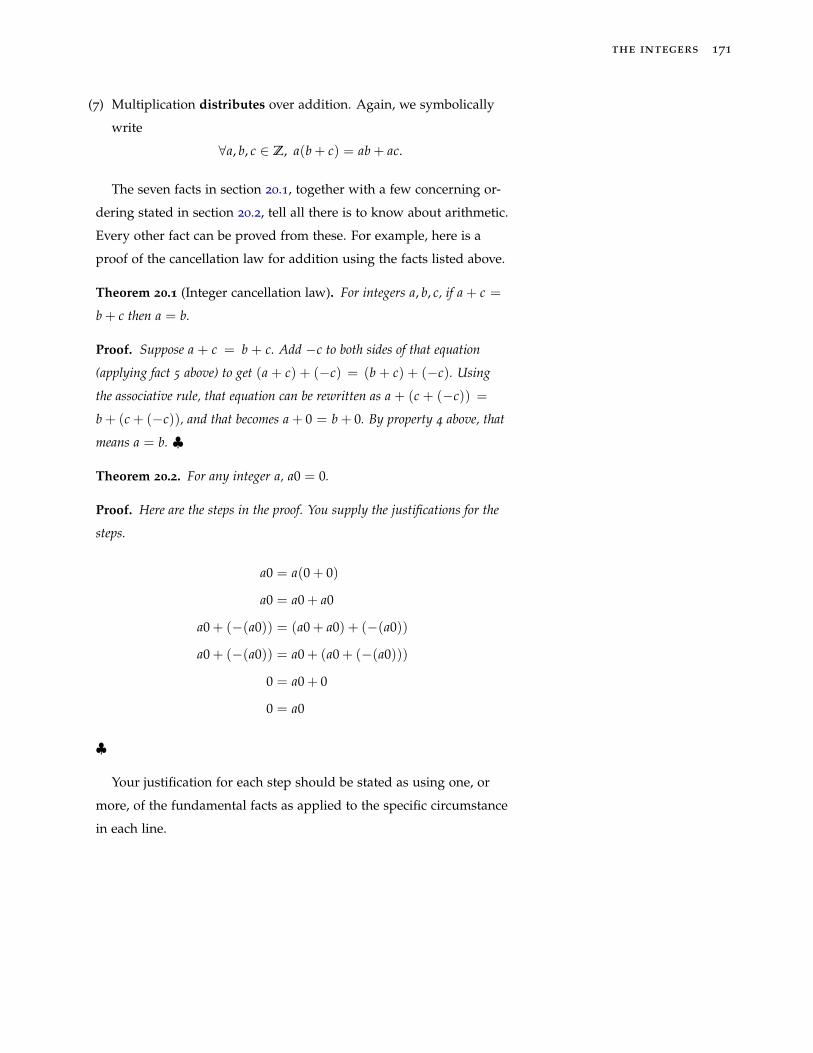
the integers 171
(7) Multiplication distributes over addition. Again, we symbolically
write
∀a, b, c ∈ Z, a(b + c) = ab + ac.
The seven facts in section 20.1, together with a few concerning or-
dering stated in section 20.2, tell all there is to know about arithmetic.
Every other fact can be proved from these. For example, here is a
proof of the cancellation law for addition using the facts listed above.
Theorem 20.1 (Integer cancellation law). For integers a, b, c, if a + c =
b + c then a = b.
Proof. Suppose a + c = b + c. Add −c to both sides of that equation
(applying fact 5 above) to get (a + c) + (−c) = (b + c) + (−c). Using
the associative rule, that equation can be rewritten as a + (c + (−c)) =
b + (c + (−c)), and that becomes a + 0 = b + 0. By property 4 above, that
means a = b. ♣
Theorem 20.2. For any integer a, a0 = 0.
Proof. Here are the steps in the proof. You supply the justifications for the
steps.
a0 = a(0 + 0)
a0 = a0 + a0
a0 + (−(a0)) = (a0 + a0) + (−(a0))
a0 + (−(a0)) = a0 + (a0 + (−(a0)))
0 = a0 + 0
0 = a0
♣
Your justification for each step should be stated as using one, or
more, of the fundamental facts as applied to the specific circumstance
in each line.
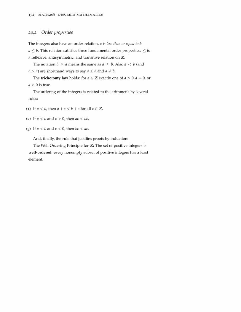
172 math208: discrete mathematics
20.2 Order properties
The integers also have an order relation, a is less than or equal to b:
a ≤ b. This relation satisfies three fundamental order properties: ≤ is
a reflexive, antisymmetric, and transitive relation on Z.
The notation b ≥ a means the same as a ≤ b. Also a < b (and
b > a) are shorthand ways to say a ≤ b and a 6= b.
The trichotomy law holds: for a ∈ Z exactly one of a > 0, a = 0, or
a < 0 is true.
The ordering of the integers is related to the arithmetic by several
rules:
(1) If a < b, then a + c < b + c for all c ∈ Z.
(2) If a < b and c > 0, then ac < bc.
(3) If a < b and c < 0, then bc < ac.
And, finally, the rule that justifies proofs by induction:
The Well Ordering Principle for Z: The set of positive integers is
well-ordered: every nonempty subset of positive integers has a least
element.
the integers 173
20.3 Exercises
Exercise 20.1. Prove that if a > 0 and b > 0, then ab > 0.
Exercise 20.2. Prove that is ab = 0, then a = 0 or b = 0. Hint: Try an
indirect proof with four cases. Case 1: Show that if a > 0 and b > 0, then
ab 6= 0. Case 2: Show that if a > 0 and b < 0, then ab 6= 0. There are two
more similar cases.
Exercise 20.3. Prove the cancellation law for multiplication: For integers
a, b, c, with c 6= 0, if ac = bc, then a = b. (Hint: Use exercise 20.2

21
The divides Relation and Primes
Given integers a and b we say that a divides b and write a|bprovided1 there is an integer c with b = ac. In that case we also say 1 That is, a divides into b evenly.
that a is a factor of b, or that a is a divisor of b, or that b is a multiple
of a. For example 3|12 since 12 = 3 · 4. Keep in mind that divides
is a relation. When you see a|b you should think is that true or false.
Don’t write things like 3|12 = 4! If a does not divide b, write a/|b. For
example, it is true2 that 3/|13. 2 Fact: 3 does not divide into 13 evenly.
21.1 Properties of divides
Here is a list of a few simple facts about the divisibility relation.
Theorem 21.1. For a, b, c ∈ Z we have
(1) a|0
(2) ±1|a
(3) If a|b, then −a|b
(4) If a|b and b|c, then a|c. So a|b is a transitive relation on Z
(5) a| − a
(6) If a|b and b 6= 0, then 0 < |a| ≤ |b|
(7) If a|1, then a = ±1
(8) If a|b and b|a, then a = ±b
176 math208: discrete mathematics
(9) a|b and a|c, then a|(mb + nc) for all m, n ∈ Z
(10) If a|b, then a|bc for all c ∈ Z
Here are the proofs of a few of these facts.
(1) Proof. For any integer a, a0 = 0, so a|0. ♣
(4) Proof. Suppose a|b and b|c. That means there are integers s, t so that
as = b and bt = c. Substituting as for b in the second equation gives
(as)t = c, which is the same as a(st) = c. That shows a|c. ♣
(9) Proof. Suppose a|b and a|c. That means there are integers s, t such
that as = b and at = c. Multiply the first equation by m and the
second by n to get a(sm) = mb and a(tn) = nc. Now add those two
equations: a(sm) + a(tn) = mb + nc. Factoring out the a on the left
shows a(sm + tn) = mb + nc, and so we see a|(mb + nc). ♣
21.2 Prime numbers
The prime integers play a central role in number theory. A positive
integer larger than 1 is said to be prime if its only positive divisors
are 1 and itself. The first few primes are 2, 3, 5, 7, 11, 13, 17, 19, 23, 29, 31, 37.
A positive integer larger than 1 which is not prime is composite.
So a composite number n has a positive divisor a which is neither 1
nor n. By part (6) of the theorem above, 1 < a < n.
So, to check if an integer n is a prime, we can trial divide it in turn
by 2, 3, 4, 5, · · · n − 1, and if we find one of these that divides n, we
can stop, concluding that n is not a prime. On the other hand, if we
find that none of those divide n, then we can conclude n is a prime.
This algorithm for checking a number for primeness can be made
more efficient. For example, there is really no need to test to see if
4 divides n if we have already determined that 2 does not divide n.
And the same reasoning shows that to test n for primeness we need
only check in to see if n is divisible by any of 2, 3, 5, 7, 11, 13 and so
on up to the largest prime less than n. For example, to test 15 for
primeness, we would trial divide by the six values 2, 3, 5, 7, 11, 13.
But even this improved algorithm can be made more efficient by the
following theorem.
the DIVIDES relation and primes 177
Theorem 21.2. Every composite number n has a divisor a, with
2 ≤ a ≤√
n.
Proof. Suppose n is a composite integer. That means n = ab where 1 <
a, b < n. Not both a and b are greater than√
n, for if so n = ab >√
n√
n = (√
n)2 = n, and that is a contradiction. ♣
So, if we haven’t found a divisor of n by the time we reach√
n,
then n must be a prime.
We can be a little more informative, as the next theorem shows.
Theorem 21.3. Every integer n > 1 is divisible by a prime.
Proof. Let n > 1 be given. The set, D, of all integers greater than 1 that
divide n is nonempty since n itself is certainly in that set. Let m be the
smallest integer in that set. Then m must be a prime since if k is an integer
with 1 < k < m and k|m, then k|n, and so k ∈ D. That is a contradiction
since m is the smallest element of D. Thus m is a prime divisor of n. ♣
Among the more important theorems in number theory is the
following.
Theorem 21.4. The set of prime integers is infinite.
Proof. Suppose that there were only finitely many primes. List them all:
2, 3, 5, 7, · · · , p. Form the number N = 1 + 2 · 3 · 5 · 7 · · · p. According
to the last theorem, there must be a prime that divides N, say q. Certainly q
also divides 2 · 3 · 5 · 7 · · · p since that is the product of all the primes, so q
is one of its factors. Hence q divides N − 2 · 3 · 5 · 7 · · · p. But that’s crazy
since N − 2 · 3 · 5 · 7 · · · p = 1. We have reached a contradiction, and so we
can conclude there are infinitely many primes. ♣
21.3 The division algorithm for integers
Theorem 21.5 (The Division Algorithm for Integers). If a, d ∈ Z, with
d > 0, there exist unique integers q and r, with a = qd + r, and 0 ≤ r < d. The quantities q and r are called the
quotient and remainder when a is
divided by d.Proof. Let S = {a− nd|n ∈ Z, and a− nd ≥ 0}. Then S 6= ∅, since
a − (−|a|)d ∈ S for sure. Thus, by the Well Ordering Principle, S has a
178 math208: discrete mathematics
least element, call it r. Say r = a − qd. Then we have a = qd + r, and
0 ≤ r. If r ≥ d, then a = (q + 1)d + (r− d), with 0 ≤ r− d contradicting
the minimality of r.
To prove uniqueness, suppose that a = q1d + r1 = q2d + r2, with
0 ≤ r1, r2 < d. Then d(q1 − q2) = r2 − r1 which implies that r2 − r1 is a
multiple of d. Since 0 ≤ r1, r2 < d, we have −d < r2 − r1 < d. Thus the
only multiple of d which r2 − r1 can possibly be is 0d = 0. So r2 − r1 = 0
which is the same thing as r1 = r2. Thus d(q1 − q2) = 0 = d0. Since d 6= 0
we can cancel d to get q1 − q2 = 0, whence q1 = q2. ♣
the DIVIDES relation and primes 179
21.4 Exercises
Exercise 21.1. Determine all the integers that 0 divides.
Exercise 21.2. Prove: For integers a, b, if a|b, then −a|b.
Exercise 21.3. Prove: For integers a, b, c, if a|b, then a|bc.
Exercise 21.4. Determine if 1297 is a prime.
Exercise 21.5. Prove or give a counterexample: If p is a prime, then 2p + 1
is a prime.
Exercise 21.6. Determine the quotient and remainder when 107653 is
divided by 22869.

22
GCD’s and the Euclidean Algorithm
The greatest common divisor of a and b, not both 0, is the
largest integer which divides both a and b. For example, the greatest
common divisor of 21 and 35 is 7. We write gcd(a, b), as shorthand
for the greatest common divisor of a and b. So gcd(35, 21) = 7.
There are several ways to find the gcd of two integers, a and b
(not both 0).
First, we could simply list all the positive divisors of a and b and
pick the largest number that appears in both lists. Notice that 1 will
appear in both lists. For the example above the positive divisors of
35 are 1, 5, 7, and 35. For 21 the positive divisors are 1, 3, 7, and 21.
The largest number appearing in both lists is 7, so gcd(35, 21) = 7.
Another way to say the same thing: If we let Da denote the set
of positive divisors of a, then gcd(a, b) = the largest number in
Da ∩ Db .
The reason gcd(0, 0) is not defined is that every positive inte-
ger divides 0, and so there is no largest integer that divides 0. From
now on, when we use the symbol gcd(a, b), we will tacitly assume
a and b are not both 0. The integers a and b can be negative. For
example if a = −34 and b = 14, then the set of positive divi-
sors of −34 is {1, 2, 17, 34} and the set of positive divisors of 14
is {1, 2, 7, 14}. The set of positive common divisors of 14 and −34 is
the set {1, 2, 17, 34} ∩ {1, 2, 7, 14} = {1, 2}. The largest number in
this set is 2 = gcd(−34, 14).
Obviously then gcd(a, b) = gcd(−a, b) since a and −a have the
182 math208: discrete mathematics
same set of positive divisors. So when computing the gcd(a, b) we
may as well replace a and b by their absolute values if one or both
happen to be negative.
Here are a few easy facts about gcd’s:
(1) If a 6= 0, then gcd(a, a) = a.
(2) gcd(a, 1) = 1.
(3) gcd(a, b) = gcd(b, a).
(4) If a 6= 0 and a|b, then gcd(a, b) = |a|.
(5) If a 6= 0, gcd(a, 0) = |a|.
If gcd(a, b) = 1, we say that a and b are relatively prime. When a
and b are relatively prime, they have no common prime divisor. For
example 12 and 35 are relatively prime.
22.1 Euclidean algorithm
It’s pretty clear that computing gcd(a, b) by listing all the positive
visors of a and all the positive divisors of b, and selecting the largest
integers that appears in both lists is not very efficient. There is a
better way of computing gcd(a, b).
Theorem 22.1. If a and b are integers (not both 0) and a = sb + t for
integers s and t, then gcd(a, b) = gcd(b, t).
Proof. To prove the theorem, we will show that the list of positive integers
that divide both a and b is identical to the list of positive integers that divide
both b and t = a − sb. So, suppose d|a and d|b. Then d|(a − sb) so
d|t. Hence d divides both b and t. On the other hand, suppose d|b and d|t.Then d|(sb + t), so that d|a. Hence d divides both a and b. It follows that
gcd(a, b) = gcd(b, t). ♣
Euclid is given the credit for discovering this fact, and its use for
computing gcd’s is called the Euclidean algorithm in his honor.
The idea is to use the theorem repeatedly until a pair of numbers
is reached for which the gcd is obvious. Here is an example of the
Euclidean algorithm in action.
gcd’s and the euclidean algorithm 183
Example 22.2. Since 14 = 1 · 10 + 4, gcd(14, 10) = gcd(10, 4).
In turn 10 = 2 · 4 + 2 so gcd(10, 4) = gcd(4, 2). Since 4 = 2 · 2,
gcd(4, 2) = gcd(2, 0) = 2. So gcd(10, 14) = 2.
The same example, presented a little more compactly, and without explic-
itly writing out the divisions, looks like
gcd(14, 10) = gcd(10, 4) = gcd(4, 2) = gcd(2, 0) = 2
At each step, the second number is replaced by the remainder when the first
number is divided by the second, and the second moves into the first spot.
The process is repeated until the second number is a 0 (which must happen
eventually since the second number never will be negative, and it goes down
by at least 1 with each repetition of the process). The gcd is then the number
in the first spot when the second spot is 0 in the last step of the algorithm.
Now, a more exciting example.
Example 22.3. Find the greatest common divisor of 540 and 252. We may
present the computations compactly, without writing1 out the divisions. We 1 Do the divisions yourself to verify theresults.
have
gcd(540, 252) = gcd(252, 36) = gcd(36, 0) = 36.
22.2 Efficiency of the Euclidean algorithm
Using the Euclidean algorithm to find gcd’s is extremely efficient.
Using a calculator with a ten digit display, you can find the gcd of
two ten digit integers in a matter of a few minutes at most using the
Euclidean algorithm. On the other hand, doing the same problem by
first finding the positive divisors of the two ten digit integers would
be a tedious project lasting several days. Some modern cryptographic
systems rely on the computation of the gcd’s of integers of hundreds
of digits. Finding the positive divisors of such large integers, even
with a computer, is, at present, a hopeless task. But a computer im-
plementation of the Euclidean algorithm will produce the gcd of
integers of hundreds of digits in the blink of an eye.
184 math208: discrete mathematics
22.3 The Euclidean algorithm in quotient/remainder form
The Euclidean algorithm can also be written out as a sequence of
divisions:
a = q1 · b + r1, 0 < r1 < b
b = q2 · r1 + r2, 0 < r2 < r1
r1 = q3 · r2 + r3, 0 < r3 < r2
... =...
rk = qk+2 · rk+1 + rk+2, 0 < rk+2 < rk+1
... =...
rn−2 = qn · rn−1 + rn, 0 < rn < rn−1
rn−1 = qn+1 · rn + 0
The sequence of integer remainders b > r1 > ... > rk > ... ≥ 0
must eventually reach 0. Let’s say rn 6= 0, but rn+1 = 0, so that
rn−1 = qn+1 · rn. That is, in the sequence of remainders, rn is the last
non-zero term. Then, just as in the examples above we see that the
gcd of a and b is the last nonzero remainder:
gcd(a, b) = gcd(b, r1) = gcd(r1, r2) = · · · = gcd(rn−1, rn)
= gcd(rn, rn+1) = gcd(rn, 0) = rn.
Let’s find gcd(317, 118) using this version of the Euclidean algorithm.
Here are the steps:
317 = 2 · 118 + 81,
118 = 1 · 81 + 37,
81 = 2 · 37 + 7,
37 = 5 · 7 + 2,
7 = 3 · 2 + 1,
2 = 2 · 1 + 0.
gcd’s and the euclidean algorithm 185
Since the last non-zero remainder is 1, we conclude that gcd(317, 118) =
1. So, in the terminology introduced above, we would say that 317
and 118 are relatively prime.
186 math208: discrete mathematics
22.4 Exercises
Exercise 22.1. Use the Euclidean algorithm to compute gcd(a, b) in each
case.
a) a = 233, b = 89 b) a = 1001, b = 13 c) a = 2457, b = 1458
d) a = 567, b = 349
Exercise 22.2. Compute gcd(987654321, 123456789).
Exercise 22.3. Write a step-by-step algorithm that implements the Eu-
clidean algorithm for finding gcd’s.
Exercise 22.4. If p is a prime, and n is any integer, what are the possible
values of gcd(p, n)?
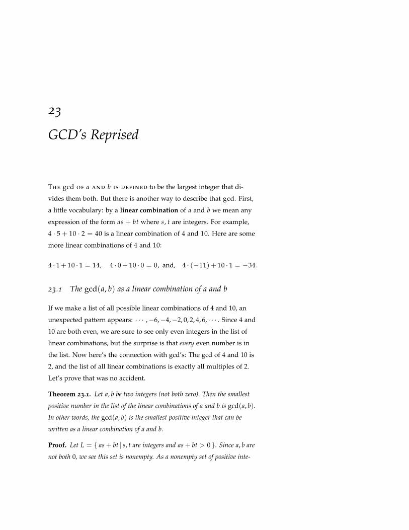
23
GCD’s Reprised
The gcd of a and b is defined to be the largest integer that di-
vides them both. But there is another way to describe that gcd. First,
a little vocabulary: by a linear combination of a and b we mean any
expression of the form as + bt where s, t are integers. For example,
4 · 5 + 10 · 2 = 40 is a linear combination of 4 and 10. Here are some
more linear combinations of 4 and 10:
4 · 1 + 10 · 1 = 14, 4 · 0 + 10 · 0 = 0, and, 4 · (−11) + 10 · 1 = −34.
23.1 The gcd(a, b) as a linear combination of a and b
If we make a list of all possible linear combinations of 4 and 10, an
unexpected pattern appears: · · · ,−6,−4,−2, 0, 2, 4, 6, · · · . Since 4 and
10 are both even, we are sure to see only even integers in the list of
linear combinations, but the surprise is that every even number is in
the list. Now here’s the connection with gcd’s: The gcd of 4 and 10 is
2, and the list of all linear combinations is exactly all multiples of 2.
Let’s prove that was no accident.
Theorem 23.1. Let a, b be two integers (not both zero). Then the smallest
positive number in the list of the linear combinations of a and b is gcd(a, b).
In other words, the gcd(a, b) is the smallest positive integer that can be
written as a linear combination of a and b.
Proof. Let L = { as + bt | s, t are integers and as + bt > 0 }. Since a, b are
not both 0, we see this set is nonempty. As a nonempty set of positive inte-
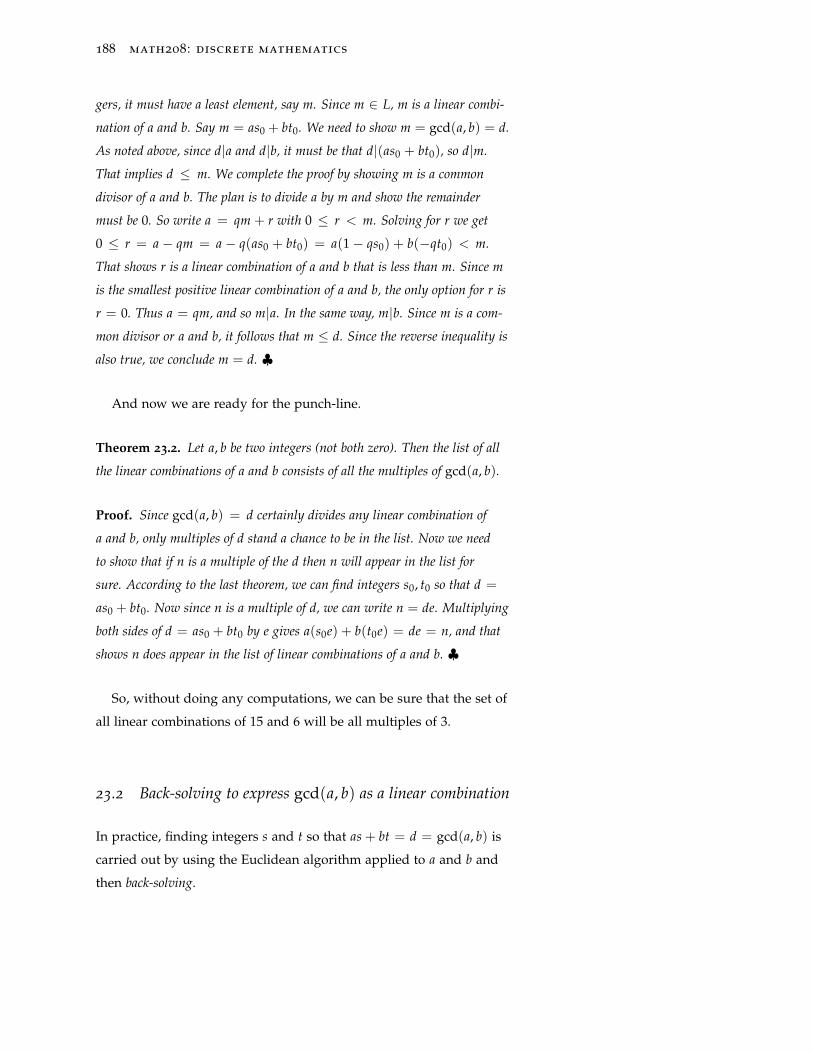
188 math208: discrete mathematics
gers, it must have a least element, say m. Since m ∈ L, m is a linear combi-
nation of a and b. Say m = as0 + bt0. We need to show m = gcd(a, b) = d.
As noted above, since d|a and d|b, it must be that d|(as0 + bt0), so d|m.
That implies d ≤ m. We complete the proof by showing m is a common
divisor of a and b. The plan is to divide a by m and show the remainder
must be 0. So write a = qm + r with 0 ≤ r < m. Solving for r we get
0 ≤ r = a − qm = a − q(as0 + bt0) = a(1− qs0) + b(−qt0) < m.
That shows r is a linear combination of a and b that is less than m. Since m
is the smallest positive linear combination of a and b, the only option for r is
r = 0. Thus a = qm, and so m|a. In the same way, m|b. Since m is a com-
mon divisor or a and b, it follows that m ≤ d. Since the reverse inequality is
also true, we conclude m = d. ♣
And now we are ready for the punch-line.
Theorem 23.2. Let a, b be two integers (not both zero). Then the list of all
the linear combinations of a and b consists of all the multiples of gcd(a, b).
Proof. Since gcd(a, b) = d certainly divides any linear combination of
a and b, only multiples of d stand a chance to be in the list. Now we need
to show that if n is a multiple of the d then n will appear in the list for
sure. According to the last theorem, we can find integers s0, t0 so that d =
as0 + bt0. Now since n is a multiple of d, we can write n = de. Multiplying
both sides of d = as0 + bt0 by e gives a(s0e) + b(t0e) = de = n, and that
shows n does appear in the list of linear combinations of a and b. ♣
So, without doing any computations, we can be sure that the set of
all linear combinations of 15 and 6 will be all multiples of 3.
23.2 Back-solving to express gcd(a, b) as a linear combination
In practice, finding integers s and t so that as + bt = d = gcd(a, b) is
carried out by using the Euclidean algorithm applied to a and b and
then back-solving.
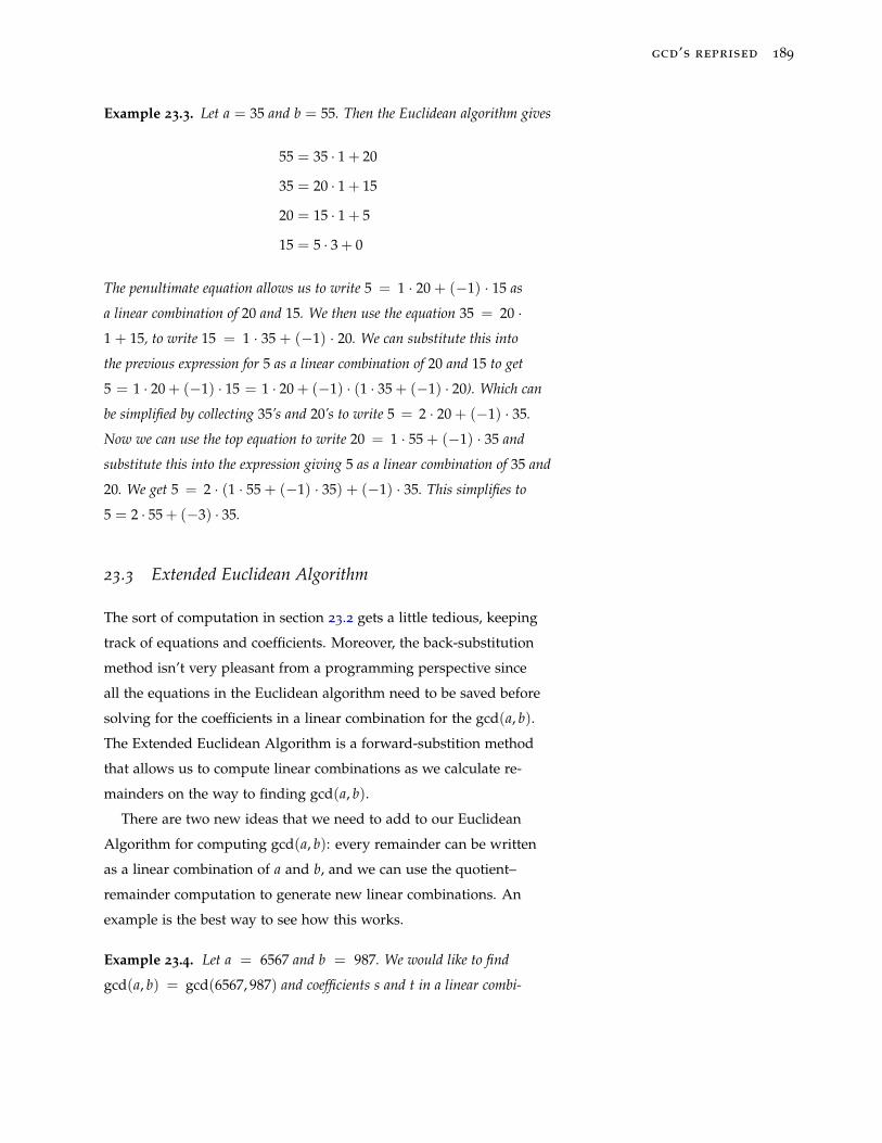
gcd’s reprised 189
Example 23.3. Let a = 35 and b = 55. Then the Euclidean algorithm gives
55 = 35 · 1 + 20
35 = 20 · 1 + 15
20 = 15 · 1 + 5
15 = 5 · 3 + 0
The penultimate equation allows us to write 5 = 1 · 20 + (−1) · 15 as
a linear combination of 20 and 15. We then use the equation 35 = 20 ·1 + 15, to write 15 = 1 · 35 + (−1) · 20. We can substitute this into
the previous expression for 5 as a linear combination of 20 and 15 to get
5 = 1 · 20 + (−1) · 15 = 1 · 20 + (−1) · (1 · 35 + (−1) · 20). Which can
be simplified by collecting 35’s and 20’s to write 5 = 2 · 20 + (−1) · 35.
Now we can use the top equation to write 20 = 1 · 55 + (−1) · 35 and
substitute this into the expression giving 5 as a linear combination of 35 and
20. We get 5 = 2 · (1 · 55 + (−1) · 35) + (−1) · 35. This simplifies to
5 = 2 · 55 + (−3) · 35.
23.3 Extended Euclidean Algorithm
The sort of computation in section 23.2 gets a little tedious, keeping
track of equations and coefficients. Moreover, the back-substitution
method isn’t very pleasant from a programming perspective since
all the equations in the Euclidean algorithm need to be saved before
solving for the coefficients in a linear combination for the gcd(a, b).
The Extended Euclidean Algorithm is a forward-substition method
that allows us to compute linear combinations as we calculate re-
mainders on the way to finding gcd(a, b).
There are two new ideas that we need to add to our Euclidean
Algorithm for computing gcd(a, b): every remainder can be written
as a linear combination of a and b, and we can use the quotient–
remainder computation to generate new linear combinations. An
example is the best way to see how this works.
Example 23.4. Let a = 6567 and b = 987. We would like to find
gcd(a, b) = gcd(6567, 987) and coefficients s and t in a linear combi-
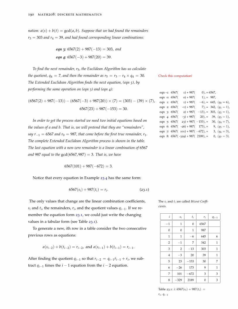
190 math208: discrete mathematics
nation: a(s) + b(t) = gcd(a, b). Suppose that we had found the remainders
r3 = 303 and r4 = 39, and had found corresponding linear combinations:
eqn 3: 6567(2) + 987(−13) = 303, and
eqn 4: 6567(−3) + 987(20) = 39.
To find the next remainder, r5, the Euclidean Algorithm has us calculate
the quotient, q4 = 7, and then the remainder as r5 = r3 − r4 × q4 = 30. Check this computation!
The Extended Euclidean Algorithm finds the next equation, (eqn 5), by
performing the same operation on (eqn 3) and (eqn 4):
(6567(2) + 987(−13))− (6567(−3) + 987(20))× (7) = (303)− (39)× (7),
6567(23) + 987(−153) = 30.
eqn -1: 6567( 1) + 987( 0), = 6567,
eqn 0: 6567( 0) + 987( 1), = 987,
eqn 1: 6567( 1) + 987( −6), = 645, (q0 = 6),
eqn 2: 6567( -1) + 987( 7), = 342, (q1 = 1),
eqn 3: 6567( 2) + 987( −13), = 303, (q2 = 1),
eqn 4: 6567( -3) + 987( 20), = 39, (q3 = 1),
eqn 5: 6567( 23) + 987( −153), = 30, (q4 = 7),
eqn 6: 6567( -26) + 987( 173), = 9, (q5 = 1),
eqn 7: 6567( 101) + 987( −672), = 3, (q6 = 3),
eqn 8: 6567( -329) + 987( 2189), = 0, (q7 = 3).
In order to get the process started we need two initial equations based on
the values of a and b. That is, we will pretend that they are “remainders”,
say r−1 = 6567 and r0 = 987, that come before the first true remainder, r1.
The complete Extended Euclidean Algorithm process is shown in the table.
The last equation with a non-zero remainder is a linear combination of 6567
and 987 equal to the gcd(6567, 987) = 3. That is, we have
6567(101) + 987(−672) = 3.
Notice that every equation in Example 23.4 has the same form:
6567(si) + 987(ti) = ri. (23.1)
The only values that change are the linear combination coefficients, The si and ti are called Bézout Coeffi-
cients.si and ti, the remainders, ri, and the quotient values qi−1. If we re-
member the equation form 23.1, we could just write the changing
values in a tabular form (see Table 23.1).i si ti ri qi−1
−1 1 0 6567
0 0 1 987
1 1 −6 645 6
2 −1 7 342 1
3 2 −13 303 1
4 −3 20 39 1
5 23 −153 30 7
6 −26 173 9 1
7 101 −672 3 3
8 −329 2189 0 3
Table 23.1: i: 6567(si) + 987(ti) =
ri , qi−1
To generate a new, ith row in a table consider the two consecutive
previous rows as equations:
a(si−2) + b(ti−2) = ri−2, and a(si−1) + b(ti−1) = ri−1.
After finding the quotient qi−1 so that ri−2 = qi−1ri−1 + ri, we sub-
tract qi−1 times the i− 1 equation from the i− 2 equation.
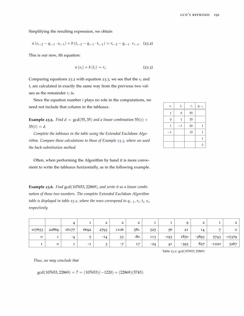
gcd’s reprised 191
Simplifying the resulting expression, we obtain
a (si−2 − qi−1 · si−1) + b (ti−2 − qi−1 · ti−1) = ri−2 − qi−1 · ri−1. (23.2)
This is our new, ith equation:
a (si) + b (ti) = ri. (23.3)
Comparing equations 23.2 with equation 23.3, we see that the si and
ti are calculated in exactly the same way from the previous two val-
ues as the remainder ri is.
Since the equation number i plays no role in the computations, we
need not include that column in the tableaux.
Example 23.5. Find d = gcd(55, 35) and a linear combination 55(s) +
35(t) = d.
si ti ri qi−1
1 0 55
0 1 35
1 −1 20 1
−1 15 1
1
3
Complete the tableaux in the table using the Extended Euclidean Algo-
rithm. Compare these calculations to those of Example 23.3, where we used
the back-substitution method.
Often, when performing the Algorithm by hand it is more conve-
nient to write the tableaux horizontally, as in the following example.
Example 23.6. Find gcd(107653, 22869), and write it as a linear combi-
nation of those two numbers. The complete Extended Euclidean Algorithm
table is displayed in table 23.2, where the rows correspond to qi−1, ri, ti, si,
respectively.
4 1 2 2 2 1 1 9 2 1 2
107653 22869 16177 6692 2793 1106 581 525 56 21 14 7 0
0 1 -4 5 -14 33 -80 113 -193 1850 -3893 5743 -15379
1 0 1 -1 3 -7 17 -24 41 -393 827 -1220 3267
Table 23.2: gcd(107653, 22869)
Thus, we may conclude that
gcd(107653, 22869) = 7 = (107653)(−1220) + (22869)(5743).
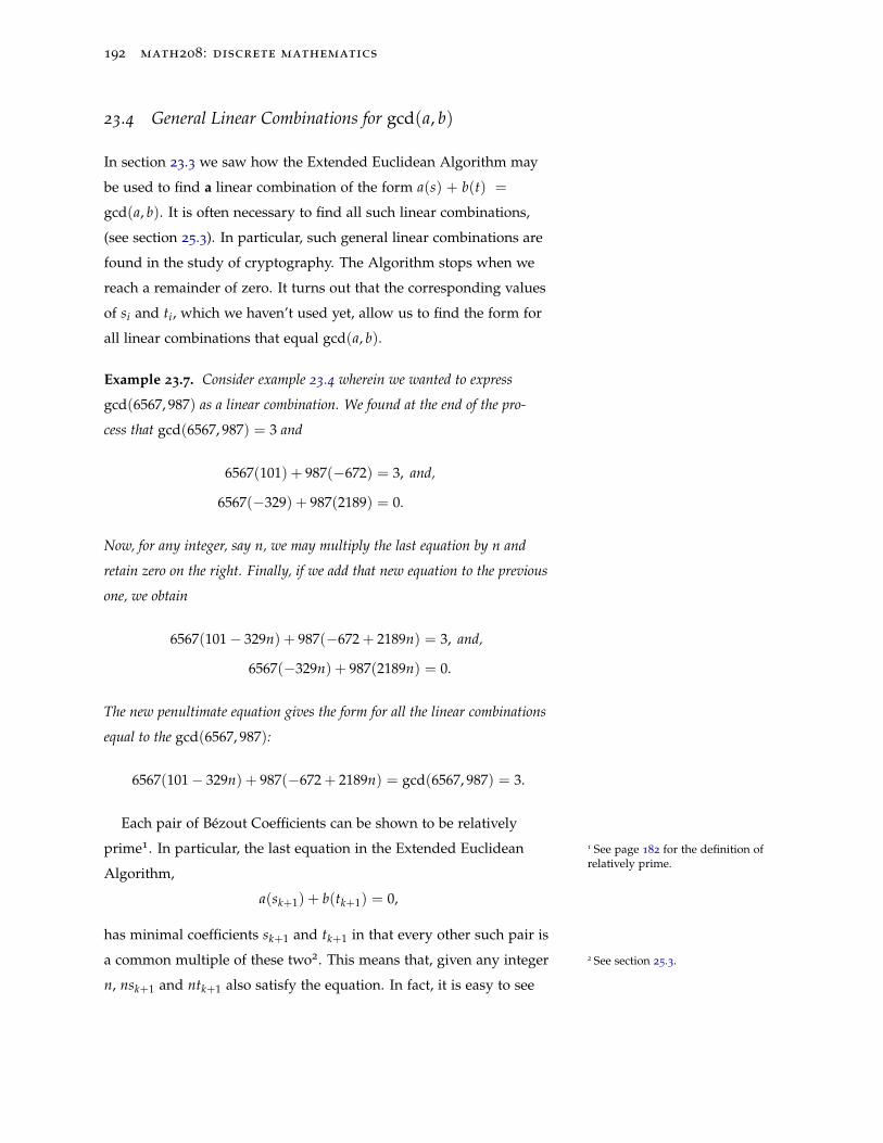
192 math208: discrete mathematics
23.4 General Linear Combinations for gcd(a, b)
In section 23.3 we saw how the Extended Euclidean Algorithm may
be used to find a linear combination of the form a(s) + b(t) =
gcd(a, b). It is often necessary to find all such linear combinations,
(see section 25.3). In particular, such general linear combinations are
found in the study of cryptography. The Algorithm stops when we
reach a remainder of zero. It turns out that the corresponding values
of si and ti, which we haven’t used yet, allow us to find the form for
all linear combinations that equal gcd(a, b).
Example 23.7. Consider example 23.4 wherein we wanted to express
gcd(6567, 987) as a linear combination. We found at the end of the pro-
cess that gcd(6567, 987) = 3 and
6567(101) + 987(−672) = 3, and,
6567(−329) + 987(2189) = 0.
Now, for any integer, say n, we may multiply the last equation by n and
retain zero on the right. Finally, if we add that new equation to the previous
one, we obtain
6567(101− 329n) + 987(−672 + 2189n) = 3, and,
6567(−329n) + 987(2189n) = 0.
The new penultimate equation gives the form for all the linear combinations
equal to the gcd(6567, 987):
6567(101− 329n) + 987(−672 + 2189n) = gcd(6567, 987) = 3.
Each pair of Bézout Coefficients can be shown to be relatively
prime1. In particular, the last equation in the Extended Euclidean 1 See page 182 for the definition ofrelatively prime.
Algorithm,
a(sk+1) + b(tk+1) = 0,
has minimal coefficients sk+1 and tk+1 in that every other such pair is
a common multiple of these two2. This means that, given any integer 2 See section 25.3.
n, nsk+1 and ntk+1 also satisfy the equation. In fact, it is easy to see
gcd’s reprised 193
that
a(nsk+1) + b(ntk+1) = 0.
Finally, to obtain the general solution, as we did in example 23.7, we
add this to the Bézout equation for the gcd(a, b), obtaining One of sk+1 and tk+1 will always be
negative!
a(sk + nsk+1) + b(tk + ntk+1) = gcd(a, b).
194 math208: discrete mathematics
23.5 Exercises
Exercise 23.1. Determine gcd(13447, 7667) and write it as a linear combi-
nation of 13447 and 7667. Try both the method of back-substitution and the
Extended Euclidean Algorithm to determine a suitable linear combination.
Exercise 23.2. What can you conclude about gcd(a, b) if there are integers
s, t with as + bt = 1?
Exercise 23.3. What can you conclude about gcd(a, b) if there are integers
s, t with as + bt = 19?
Exercise 23.4. What can you conclude about gcd(a, b) if there are integers
s, t with as + bt = 18?
24
The Fundamental Theorem of Arithmetic
The Fundamental Theorem of Arithmetic states the fa-
miliar fact that every positive integer greater than 1 can be written
in exactly one way as a product of primes. For example, the prime
factorization of 60 is 22 · 3 · 5, and the prime factorization of 625 is
54. The factorization of 60 can be written is several different ways:
60 = 2 · 2 · 3 · 5 = 5 · 2 · 3 · 2, and so on. The order in which the factors
are written does not matter. The factorization of 60 into primes will
always have two 2’s, one 3, and one 5. One more example: The fac-
torization if 17 consists of the single factor 17. In the standard form of
the factorization of an integer greater than 1, the primes are written
in order of size, and exponents are used for primes that are repeated
in the factorization. So, for example, the standard factorization of 60
is 60 = 22 · 3 · 5.
24.1 Prime divisors
Before proving the Fundamental Theorem of Arithmetic, we will
need to assemble a few facts.
Theorem 24.1. If n|ab and n and a are relatively prime, then n|b.
Proof. Suppose n|ab and that gcd(n, a) = 1. We can find integers s, t
such that ns + at = 1. Multiply both sides of that equation by b to get
nsb + abt = b. Since n divides both terms on the left side of that equation, it
divides their sum, which is b. ♣
196 math208: discrete mathematics
One consequence of this theorem is that if a prime divides a prod-
uct of some integers, then it must divide one of the factors. That is so
since if a prime does not divide an integer, then it is relatively prime
to that integer. That is useful enough to state as a theorem.
Theorem 24.2. If p is a prime, and p|a1a2 · · · an, then p|aj for some j =
1, 2, · · · , n.
24.2 Proving the Fundamental Theorem
Theorem 24.3 (Fundamental Theorem of Arithmetic). If n > 1 is an
integer, then there exist prime numbers p1 ≤ p2 ≤ ... ≤ pr such that
n = p1 p2 · · · pr and there is only one such prime factorization of n.
Proof. There are two things to prove: (1) every n > 1 can be written in
at least one way as a product of primes (in increasing order) and (2) there
cannot be two different such expressions equal to n.
We will prove these by induction. For the basis, we see that 2 can be
written as a product of primes (namely 2 = 2) and, since 2 is the smallest
prime, this is the only way to write 2 as a product of primes.
For the inductive step, suppose every integer from 2 to k can be writ-
ten uniquely as a product of primes. Now consider the number k + 1. We
consider two cases:
(1) If k + 1 is a prime then k + 1 is already an expression for k + 1 as a
product of primes. There cannot be another expression for k + 1 as a
product of primes, for if k + 1 = pm with p a prime, then p|k + 1 and p
and k + 1 both primes tells us p = k + 1, and so m = 1.
(2) If k + 1 is not a prime, then we can write k + 1 = ab with 2 ≤ a, b ≤ k.
By the inductive hypothesis, each of a and b can be written as prod-
ucts of primes, say a = p1 p2 · · · ps and b = q1q2 · · · qt. That means
k + 1 = p1 p2 · · · psq1q2 · · · qt, and we can rearrange the primes in
increasing order. To complete the proof, we need to show k + 1 can-
not be written in more than one way as a product of an increasing
list of primes. So suppose k + 1 has two different such expressions:
k + 1 = u1u2 · · · ul = v1v2 · · · vm. Since u1|v1v2 · · · vm, u1 must
divide some one of the vi’s and since u1 and that vi are both primes,
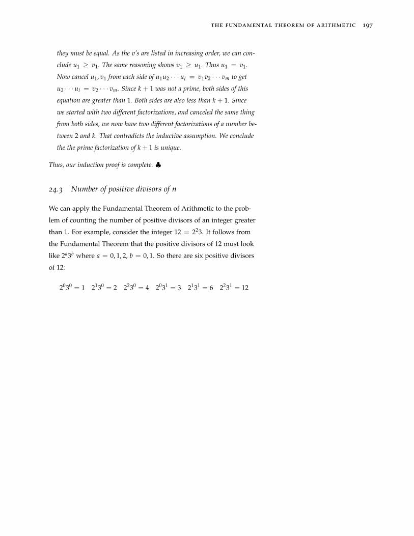
the fundamental theorem of arithmetic 197
they must be equal. As the v’s are listed in increasing order, we can con-
clude u1 ≥ v1. The same reasoning shows v1 ≥ u1. Thus u1 = v1.
Now cancel u1, v1 from each side of u1u2 · · · ul = v1v2 · · · vm to get
u2 · · · ul = v2 · · · vm. Since k + 1 was not a prime, both sides of this
equation are greater than 1. Both sides are also less than k + 1. Since
we started with two different factorizations, and canceled the same thing
from both sides, we now have two different factorizations of a number be-
tween 2 and k. That contradicts the inductive assumption. We conclude
the the prime factorization of k + 1 is unique.
Thus, our induction proof is complete. ♣
24.3 Number of positive divisors of n
We can apply the Fundamental Theorem of Arithmetic to the prob-
lem of counting the number of positive divisors of an integer greater
than 1. For example, consider the integer 12 = 223. It follows from
the Fundamental Theorem that the positive divisors of 12 must look
like 2a3b where a = 0, 1, 2, b = 0, 1. So there are six positive divisors
of 12:
2030 = 1 2130 = 2 2230 = 4 2031 = 3 2131 = 6 2231 = 12
198 math208: discrete mathematics
24.4 Exercises
Exercise 24.1. Determine the prime factorization of 345678.
Exercise 24.2. Determine the prime factorization of 1016.
Exercise 24.3. List all the positive divisors of 1016.
Exercise 24.4. How many positive divisors does 345678 have?
25
Linear Diophantine Equations
Consider the following problem:
Al buys some books at $25 each, and some magazines at $3 each.
If he spent a total of $88, how many books and how many magazines
did Al buy? At first glance, it does not seem we are given enough
information to solve this problem. Letting x be the number of books
Al bought, and y the number of magazines, then the equation we
need to solve is 25x + 3y = 88. Thinking back to college algebra
days, we recognize 25x + 3y = 88 as the equation of a straight line
in the plane, and any point along the line will give a solution to the
equation. For example, x = 0 and y = 883 is one solution. But, in
the context of this problem, that solution makes no sense because Al
cannot buy a fraction of a magazine. We need a solution in which x
and y are both integers. In fact, we need even a little more care than
that. The solution x = −2 and y = 46 is also unacceptable since Al
cannot buy a negative number of books. So we really need solutions
in which x and y are both nonnegative integers. The problem can be
solved by brute force: If x = 0, y is not an integer. If x = 1, then
y = 21, so that is one possibility. If x = 2, y is not an integer. If
x = 3, y is not an integer. And, if x is 4 or more, then y would have
to be negative. So, it turns out there is only one possible solution: Al
bought one book, and 21 magazines.
200 math208: discrete mathematics
25.1 Diophantine equations
The above question is an example of a Diophantine problem. Pro-
nounce Diophantine as dee-uh-FAWN-teen or dee-uh-FAWN-tine, or,
the more common variations, die-eh-FAN-teen or die-eh-FAN-tine. . In For a modern pronunciation of Dio-
phantus’s name (∆ιoφαντoζ) see http:
//www.pronouncenames.com/Diophantusgeneral, problems in which we are interested in finding solutions in
which the variables are to be integers are called Diophantine prob-
lems.
In this chapter we will learn how to easily find the solutions to
all linear Diophantine equations: ax + by = c where a, b, c are given
integers. To show some of the subtleties of such problems, here are
two more examples:
(1) Al buys some books at $24 each, and some magazines at $3 each.
If he spent a total of $875, how many books and how many maga-
zines did Al buy? For this question we need to solve the Diophan-
tine equation 24x + 3y = 875. In this case there are no possible
solutions. For any integers x and y, the left-hand side will be a
multiple of 3 and so cannot be equal to 875 which is not a multiple
of 3.
(2) Al buys some books at $26 each, and some magazines at $3 each.
If he spent a total of $157, how many books and how many mag-
azines did Al buy? Setting up the equation as before, we need to
solve the Diophantine equation 26x + 3y = 175. A little trial and
error, testing x = 0, 1, 2, 3, and so on shows there are two possible
answers this time: (x, y) ∈ {(2, 35), (5, 9)}.
25.2 Solutions and gcd(a, b)
Determining all the solutions to ax + by = c is closely connected
with the idea of gcd’s. One connection is theorem 23.1. Here is how
solutions of ax + by = c are related.
Theorem 25.1. ax + by = c has a solution in the integers if and only if
gcd(a, b) divides c.
So, for example, 9x + 6y = 211 has no solutions (in the integers)
while 9x + 6y = 213 does have solutions. To find a solution to the last
linear diophantine equations 201
equation, apply the Extended Euclidean Algorithm method to write
the gcd(9, 6) as a linear combination of 9 and 6 (actually, this one is
easy to do by sight): 9 · 1 + 6 · (−1) = 3, then multiply both sides by
213/gcd(9, 6) = 213/3 = 71 to get (71)9 + (−71)6 = 213. That shows
x = 71, y = −71 is a solution to 9x + 6y = 213.
But that is only one possible solution. When a linear Diophantine
equation has one solution it will have infinitely many. In the example
above, another solution will be x = 49 and y = −38. Checking shows
that (49)9 + (−38)6 = 213.
25.3 Finding all solutions
There is a simple recipe for all solutions, once one particular solution
has been found.
Theorem 25.2. Let d = gcd(a, b). Suppose x = s and y = t is one
solution to ax + by = c. Then all solutions are given by
x = s + kbd
and y = t− kad
where, k = any integer.
Proof. It is easy to check that all the displayed x, y pairs are solutions
simply by plugging in:
a(
s + kbd
)+ b
(t− k
ad
)= as +
abkd
+ bt− abkd
= as + bt = c.
Checking that the displayed formulas for x and y give all possible solu-
tions is trickier. Let’s assume a 6= 0. Now suppose x = u and y = v
is a solution. That means au + bv = c = as + bt. It follows that
a(u− s) = b(t− v). Divide both sides of that equation by d to get
ad(u− s) =
bd(t− v).
That equation showsad
∣∣∣∣ bd(t− v). Since
ad
andbd
are relatively prime, we
conclude thatad
∣∣∣∣ (t− v). Let’s say kad= t− v. Rearrange that equation to
get
v = t− kad
.
202 math208: discrete mathematics
Next, replacing t− v in the equationad(u− s) =
bd(t− v) with k
ad
gives
ad(u− s) =
bd(t− v) =
bd
(k
ad
).
Sincead6= 0, we can cancel that factor. So, we have
u− s = kbd
so that u = s + kbd
.
That proves the solution x = u, y = v is given by the displayed formulas.
♣
25.4 Examples
Example 25.3. Determine all the solutions to 221x + 91y = 39.
Using the Extended Euclidean Algorithm method, we learn that gcd(221, 91) =
13 and since 13|39, the equation will have infinitely many solutions. The
Extended Euclidean Algorithm table provides a linear combination of 221
and 91 equal to 13: 221(−2) + 91(5) = 13. Multiply both sides by
3 and we get 221(−6) + 91(15) = 39. So one particular solution to
221x + 91y = 39 is x = −6, y = 15. According the the theorem above, all
solutions are given by
x = −6 + k9113
= −6 + 7k and y = 15− k22113
= 15− 17k,
where k is any integer.
Example 25.4. Armand buys some books for $25 each and some cd’s for $12
each. If he spent a total of $331, how many books and how many cd’s did he
buy?
Let x = the number of books, and y = the number of cd’s. We need to
solve 25x + 12y = 331. The gcd of 25 and 12 is 1, and there is an obvious
linear combination of 25 and 12 which equals 1: 25(1) + 12(−2) = 1.
Multiplying both sides by 331 gives 25(331) + 12(−662) = 331. So one
particular solution to 25x + 12y = 331 is x = 331 and y = −662. Of
course, that won’t do for an answer to the given problem since we want
x, y ≥ 0. To find the suitable choices for x and y, let’s look at all the possible
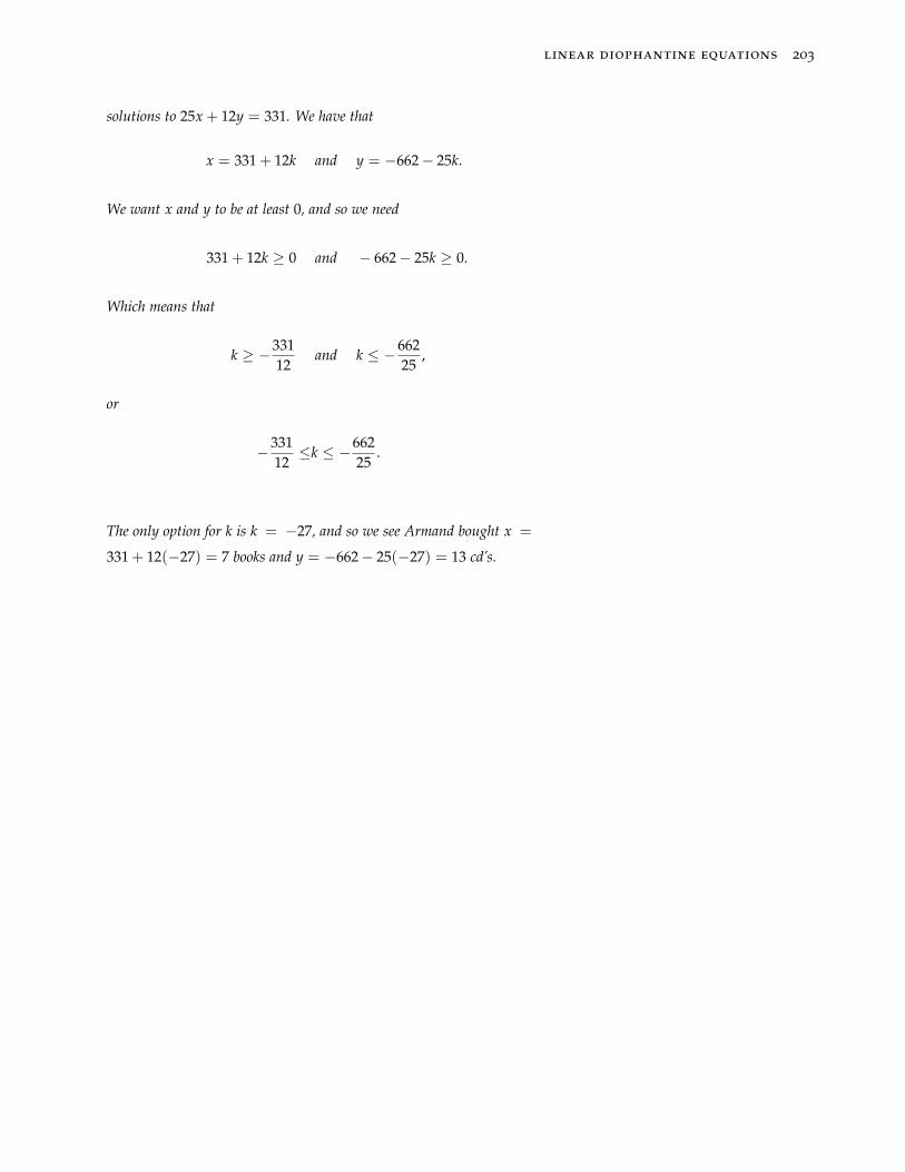
linear diophantine equations 203
solutions to 25x + 12y = 331. We have that
x = 331 + 12k and y = −662− 25k.
We want x and y to be at least 0, and so we need
331 + 12k ≥ 0 and − 662− 25k ≥ 0.
Which means that
k ≥ −33112
and k ≤ −66225
,
or
−33112≤k ≤ −662
25.
The only option for k is k = −27, and so we see Armand bought x =
331 + 12(−27) = 7 books and y = −662− 25(−27) = 13 cd’s.
204 math208: discrete mathematics
25.5 Exercises
Exercise 25.1. Find all integer solutions to 21x + 48y = 8.
Exercise 25.2. Find all integer solutions to 21x + 48y = 9.
Exercise 25.3. Sal sold some ceramic vases for $59 each, and a number of
ash trays for $37 each. If he took in a total of $4270, how many of each item
did he sell?
26
Modular Arithmetic
Karl Friedrich Gauss made the important discovery of modular
arithmetic. Modular arithmetic is also called clock arithmetic, and we
are actually used to doing modular arithmetic all the time (pun in-
tended). For example, consider the question If it is 7 o’clock now, what
time will it be in 8 hours?. Of course the answer is 3 o’clock, and we
found the answer by adding 7 + 8 = 15, and then subtracting 12 to
get 15− 12 = 3. Actually, we are so accustomed to that sort of cal-
culation, we probably just immediately blurt out the answer without
stopping to think how we figured it out. But trying a less familiar
version of the same sort of problem makes it plain exactly what we
needed to do to answer such questions: If it is 7 o’clock now, what time
will it be in 811 hours? To find out, we add 7 + 811 = 818, then divide
that by 12, getting 818 = (68)(12) + 2, and so we conclude it will be
2 o’clock. The general rule is: to find the time h hours after t o’clock,
add h + t, divide by 12 and take the remainder.
There is nothing special about the number 12 in the above dis-
cussion. We can imagine a clock with any integer number of hours
(greater than 1) on the clock. For example, consider a clock with 5
hours. What time will it be 61 hours after 2 o’clock. Since 61 + 2 =
63 = (12)(5) + 3, the answer is 3 o’clock.
In the general case, if we have a clock with m hours, then the time
h hours after t o’clock will be the remainder when t + h is divided by
m.
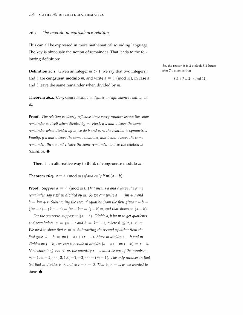
206 math208: discrete mathematics
26.1 The modulo m equivalence relation
This can all be expressed in more mathematical sounding language.
The key is obviously the notion of remainder. That leads to the fol-
lowing definition:
So, the reason it is 2 o’clock 811 hours
after 7 o’clock is that
811 + 7 ≡ 2 (mod 12)
Definition 26.1. Given an integer m > 1, we say that two integers a
and b are congruent modulo m, and write a ≡ b (mod m), in case a
and b leave the same remainder when divided by m.
Theorem 26.2. Congruence modulo m defines an equivalence relation on
Z.
Proof. The relation is clearly reflexive since every number leaves the same
remainder as itself when divided by m. Next, if a and b leave the same
remainder when divided by m, so do b and a, so the relation is symmetric.
Finally, if a and b leave the same remainder, and b and c leave the same
remainder, then a and c leave the same remainder, and so the relation is
transitive. ♣
There is an alternative way to think of congruence modulo m.
Theorem 26.3. a ≡ b (mod m) if and only if m|(a− b).
Proof. Suppose a ≡ b (mod m). That means a and b leave the same
remainder, say r when divided by m. So we can write a = jm + r and
b = km + r. Subtracting the second equation from the first gives a− b =
(jm + r)− (km + r) = jm− km = (j− k)m, and that shows m|(a− b).
For the converse, suppose m|(a − b). Divide a, b by m to get quotients
and remainders: a = jm + r and b = km + s, where 0 ≤ r, s < m.
We need to show that r = s. Subtracting the second equation from the
first gives a − b = m(j − k) + (r − s). Since m divides a − b and m
divides m(j− k), we can conclude m divides (a− b)− m(j− k) = r − s.
Now since 0 ≤ r, s < m, the quantity r − s must be one of the numbers
m− 1, m− 2, · · · , 2, 1, 0,−1,−2, · · · − (m− 1). The only number in that
list that m divides is 0, and so r − s = 0. That is, r = s, as we wanted to
show. ♣
modular arithmetic 207
26.2 Equivalence classes modulo m
The equivalence class of an integer a with respect to congruence
modulo m will be denoted by [a], or [a]m in case we are employing
more than one number m as a modulus. In other words, [a] is the set
of all integers that leave the same remainder as a when divided by
m. Or, another way to say the same thing, [a] comprises all integers
b such that b − a is a multiple of m. That means b − a = km, or
b = a + km.
That last version is often the easiest way to think about the inte- For example, the equivalence class of 7
modulo 11 would be
[7] = {· · · ,−15,−4, 7, 18, 29, 40, · · · }.gers that appear in [a]: start with a and add and subtract any number
of m’s.
We know that the distinct equivalence classes partition Z. Since di-
viding an integer by m leaves one of 0, 1, 2, · · · , m− 1 as a remainder,
we can conclude that there are exactly m equivalence classes modulo
m. In particular, [0], [1], [2], [3], ...[m − 1] is a list of all the different
equivalence classes modulo m. It is traditional when working with �
modular arithmetic to drop the [ ] symbols denoting the equivalence
classes, and simply write the representatives. So we would say, mod-
ulo m, there are m numbers: 0, 1, 2, 3, · · · , m − 1. But keep in mind
that each of those numbers really represents a set, and we can replace
any number in that list with another equivalent to it modulo m. For
example, we can replace the 0 by m. The list 1, 2, 3 · · · , m− 1, m still
consists of all the distinct values modulo m.
26.3 Modular arithmetic
One reason the relation of congruence modulo m useful is that addi-
tion and multiplication of numbers modulo m acts in many ways just
like arithmetic with ordinary integers.
Theorem 26.4. If a ≡ c (mod m), and b ≡ d (mod m), then a + b ≡c + d (mod m) and ab ≡ cd (mod m).
Proof. Suppose a ≡ c (mod m) and b ≡ d (mod m). Then there exist
integers k and l with a = c + km and b = d + lm. So a + b = c + km +
d + lm = (c + d) + (k + l)m. This can be rewritten as (a + b)− (c + d) =
208 math208: discrete mathematics
(k + l)m, where k + l ∈ Z. So a + b ≡ c + d (mod m). The other part is
done similarly. ♣
Example 26.5. What is the remainder when 1103 + 112 is divided by 11?
We can answer this problem in two different ways. We could add 1103 and
112, and then divide by 11. Or, we could determine the remainders when
each of 1103 and 112 is divided by 11, then add those remainders before
dividing by 11. The last theorem promises us the two answers will be the
same. In fact 1103 + 112 = 1215 = (110)(11) + 5 so that 1103 +
112 ≡ 5 (mod 11). On the other hand 1103 = (100)(11) + 3 and
112 = (10)(11) + 2, so that 1103 + 112 ≡ 3 + 2 ≡ 5 (mod 11).
Example 26.6. A little more impressive is the same sort of problem with
operation of multiplication: what is the remainder when (1103)(112) is
divided by 11? The calculation looks like (1103)(112) ≡ (3)(2) ≡ 6
(mod 11).
Example 26.7. For a really awe inspiring example, let’s find the re-
mainder when 1103112 is divided by 11. In other words, we want to find
x = 0, 1, 2, · · · 10 so that 1103112 ≡ x (mod 11).
Now 1103112 is a pretty big number (in fact, since log 1103112 =
112 log 1103 = 340.7 · · · , the number has 341 digits). In order to solve
this problem, let’s start by thinking small: Let’s compute 1103n, for n =
1, 2, 3, · · · .
11031 ≡ 1103 ≡ 3 (mod 11)
11032 ≡ 32 ≡ 9 (mod 11)
11033 ≡ 1103(11032) ≡ 3(9) ≡ 27 ≡ 5 (mod 11)
11034 ≡ (1103)(11033) ≡ 3(5) ≡ 15 ≡ 4 (mod 11)
11035 ≡ (1103)(11034) ≡ 3(4) ≡ 12 ≡ 1 (mod 11)
Now that last equation is very interesting. It says that whenever we see
11035 we may just as well write 1 if we are working modulo 11. And now
we see there is an easy way to determine 1103112 modulo 11:
1103112 ≡ 11035(22)+2 ≡ (11035)22(11032) ≡ 122(9) ≡ 9 (mod 11)
modular arithmetic 209
The sort of computation in example 26.7 appears to be just a cu-
riosity, but in fact the last sort of example forms the basis of one
version of public key cryptography. Computations of exactly that
type (but with much larger integers) are made whenever you log into
a secure Internet site. It’s reasonable to say that e-commerce owes its
existence to the last theorem.
While modular arithmetic in many ways behaves like ordinary
arithmetic, there are some differences to watch for. One important
difference is the familiar rule of cancellation: in ordinary arithmetic, if �
ab = ac and a 6= 0, then b = c. This rule fails in modular arithmetic.
For example, 3 6≡ 0 (mod 6) and (3)(5) ≡ (3)(7) (mod 6), but 5 6≡ 7
(mod 6).
26.4 Solving congruence equations
Solving congruence equations is a popular sport. Just as with regular
arithmetic with integers, if we want to solve a + x ≡ b (mod m),
we can simply set x ≡ b − a (mod m). So, for example, solving
55 + x ≡ 11 (mod 6) we would get x ≡ 11− 55 ≡ −44 ≡ 4 (mod 6).
Equations involving multiplication, such as ax ≡ b (mod m), are
much more interesting. If the modulus m is small, equations of this
sort can be solved by trial-and-error: simply try all possible choices
for x. For example, testing x = 0, 1, 2, 3, 4, 5, 6 in the equation 4x ≡ 5
(mod 7), we see x ≡ 3 (mod 7) is the only solution. The equation
4x ≡ 5 (mod 8) has no solutions at all. And the equation 2x ≡ 4
(mod 6) has x ≡ 2, 5 (mod 6) for solutions.
Trial-and-error is not a suitable approach for large values of m.
There is a method that will produce all solutions to ax ≡ b (mod m).
It turns out that such equations are really just linear Diophantine
equations in disguise, and that is the key to the proof of the following
theorem.This is why 4x ≡ 5 (mod 7) has a
solution: gcd(4, 7) = 1 and 1|5. And,
why 4x ≡ 5 (mod 8) has no solutions:
gcd(4, 8) = 4, but 4/|5.
Theorem 26.8. The congruence ax ≡ b (mod m) can be solved for x if
and only if d = gcd(a, m) divides b.
Proof. Solving ax ≡ b (mod m) is the same as finding x so that
m|(ax − b) and that’s the same as finding x and y so that ax − b = my.
210 math208: discrete mathematics
Rewriting that last equation in the form ax + (−m)y = b, we can see
solving ax ≡ b (mod m) is the same as solving the linear Diophantine
equation ax + (−m)y = b. We know that equation has a solution if and
only if gcd(a, m)|b, so that proves the theorem. ♣
The theorem also shows that 2x ≡ 4 (mod 6) has a solution
since gcd(2, 6) = 2 and 2|4. But why does this last equation have
two solutions? The answer to that is also provided by the results
concerning linear Diophantine equations.
Let gcd(a, m) = d. The solutions to ax ≡ b (mod m) are the
same as the solutions for x to ax + (−m)y = b. Supposing that last
equation has a solution with x = s, then we know all possible choices
of x are given by x = s + k md . So if x = s is one solution to ax ≡ b
(mod m), then all solutions are given by x = s + k md , where k is any
integer. In other words, all solutions are given by x ≡ s (mod )m d,
and so there are d solutions modulo m,
Example 26.9. Let’s find all the solutions to 2x ≡ 4 (mod 6). Since x = 2
is obviously one solution, we see all solutions are given by x = 2 + k 62 =
2 + 3k, where k is any integer. When k = 0, 1 we get x = 2, 5, and other
values of k repeat these two modulo 6. Looking at the solutions written as
x = 2 + k 62 = 2 + 3k, we can see another way to express the solutions
would be as x ≡ 2 (mod 3).
Example 26.10. Find all solutions to 42x ≡ 35 (mod 91).
Using the continued fraction method (or just staring at the numbers
42 and 91 long enough) we see gcd(91, 42) = 7 and, since 7|35, the
equation will have a solution. In fact, since gcd(42, 91) = 7, there are
going to be seven solutions modulo 91. All we need is to find one partic-
ular solution, then the others will all be easy to determine. Again using
the continued fraction method (or just playing with 42 and 91 a little bit)
we discover (42)(−2) + (91)(1) = 7 = gcd(42, 91). Multiplying by 5
gives (42)(−10) + (91)(5) = 35. The only thing we care about is that
x = −10 is one solution to 42x ≡ 35 (mod 91). As above, it follows that
all solutions are given by x ≡ −10(
(mod ) 91gcd(42,91)
). That’s the same
as x ≡ −10 (mod 13), or, even more neatly, x ≡ 3 (mod 13). In other
words, the solutions are 3, 16, 29, 42, 55, 68, 81 modulo 91.
modular arithmetic 211
26.5 Exercises
Exercise 26.1.
(a) On a military (24-hour) clock, what time is it 3122 hours after 16 hun-
dred hours?
(b) What day of the week is it 3122 days after a Monday?
(c) What month is it 3122 months after November?
Exercise 26.2. List the integers in [7]11.
Exercise 26.3. In a listing of the five equivalence classes modulo 5, four of
the values are 1211, 218, −100, and −3333. What are the possible choices
for the fifth value?
Exercise 26.4. Determine n between 0 and 24 such that
2311 + 3912 ≡ n (mod 25).
Exercise 26.5. Determine n between 0 and 24 such that
(2311)(3912) ≡ n (mod 25).
Exercise 26.6. Determine n between 0 and 8 such that 11112222 ≡ n
(mod 9).
Exercise 26.7. Solve: 4x ≡ 3 (mod 7).
Exercise 26.8. Solve 11x ≡ 8 (mod 57).
Exercise 26.9. Solve: 14x ≡ 3 (mod 231).
Exercise 26.10. Solve 8x ≡ 16 (mod 28)
Exercise 26.11. Solve: 91x ≡ 189 (mod 231)
Exercise 26.12. Let d = gcd(a, m), and let s be a solution to ax ≡ b
(mod m).
(a) Show that if ax ≡ b (mod m), then there is an integer r with 0 ≤ r < d
and x = s + r(m
d).
(b) If 0 ≤ r1 < r2 < d, then the numbers x1 = s + r1(m
d)
and x2 =
s + r2(m
d)
are not congruent modulo m.

27
Integers in Other Bases
The usual way of writing integers is in terms of groups of ones
(units), and groups of tens, and groups of tens of tens (hundreds),
and so on. Thus 237 stands for 7 units plus 3 tens and 2 hundreds, or
2(102) + 3(10) + 7. This is the familiar decimal notation for numbers
(deci = ten). But there is really nothing special about the number ten
here, and it could be replaced by any integer bigger than one. That is,
we could use say 7 the way 10 was used above to describe a number.
Thus we would specify how many units, how many 7’s and 72’s and
73’s, and so on are needed to make up the number. When a num-
ber is expressed in this fashion with b in place of the 10, the result is
called the base-b expansion (or radix-b expansion) of the integer.
For example, the decimal integer 132, is made up of two 72’s,
four 7’s and finally six units. Thus we express the base ten number
132 as 246 in base 7, or as 2467, the little 7 indicating the base. For
small numbers, with a couple of minutes practice, conversion from
base 10 (decimal) to other bases, and back again can be carried out
mentally. For larger numbers, mental arithmetic will prove a little
awkward. Luckily there is a handy algorithm to do the conversion
automatically.
27.1 Converting to and from base-10
For base 10 integers, we use the decimal digits: 0, 1, 2, 3, 4, 5, 6, 7, 8, 9.
In general, for base b, the digits will be 0, 1, 2, 3 · · · , b − 1. So, for
example, a base 7 numbers use digits 0, 1, 2, 3, 4, 5, 6.
214 math208: discrete mathematics
Conversion from the base b expansion of a number to its decimal
version is a snap: For example, the meaning of 23025 is
23025 = 2 · 53 + 3 · 52 + 0 · 5 + 2 = 2(125) + 3(25) + 0(5) + 2 = 327
That sort of computation is so easy because we have been prac-
ticing base 10 arithmetic for so many years. If we were as good at
arithmetic in some base b, then conversion from base 10 to base b
would be just as simple. But, lacking that comfort with base b arith-
metic, we need to describe the conversion algorithm from decimal to
base b a little more formally. Here’s the idea.
Suppose we have a decimal number n that we want to convert to
some base b. Let’s say the base b expansion is dkdk−1 · · · d2d1d0, with
the base b digits between 0 and b− 1. That means
n = dk · bk + dk−1 · bk−1 + · · ·+ d2 · b2 + d1 · b + d0
Now, if we divide n by b, we can see the equation above tells us
n = (dk · bk−1 + dk−1 · bk−2 + · · ·+ d2 · b + d1)b + d0
So the quotient is q = dk · bk−1 + dk−1 · bk−2 + · · ·+ d2 · b + d1, and
and the remainder is the base b digit d0 of n. So we have found the
units digit in the base b expansion of n. If we repeat that process on
the quotient q, the result is
q = (dk · bk−2 + dk−1 · bk−3 + · · ·+ d2)b + d1
so the next base b digit, d1 appears as the remainder. Continuing in
this fashion, the base b expansion is produced one digit at a time.
Briefly, to convert a positive decimal integer n to its base b repre-
sentation, divide n by b, to find the quotient and the remainder. That
remainder will be needed units digit. Then divide the quotient by b
again, to get a new quotient and a new remainder. That remainder
gives the next base b digit. Then divide the new quotient by b again,
and so on. In this way producing the base b digits one after the other.

integers in other bases 215
Example 27.1. To convert 14567 from decimal to base 5, the steps are:
14567 = 2913 · 5 + 2,
2913 = 582 · 5 + 3,
582 = 116 · 5 + 2,
116 = 23 · 5 + 1,
23 = 4 · 5 + 3,
4 = 0 · 5 + 4.
So, we see that 14567 = 4312325.
27.2 Converting between non-decimal bases
Example 27.2. Convert n = 33557 to base 5.
The least confusing way to do such a problem would be to convert n
from base 7 to base 10, and then convert the base 10 expression for n to
base 5. This method allows us to do all our work in base 10 where we are
comfortable. The computations start with:
n = 3 · 73 + 3 · 72 + 5 · 7 + 5 = 1216.
Then, we calculate:
1216 = 243 · 5 + 1,
243 = 48 · 5 + 3,
48 = 9 · 5 + 3,
9 = 1 · 5 + 4,
1 = 0 · 5 + 1.
So, we have 33557 = 143315.
An alternative method, not for the faint of heart, is convert di-
rectly from base 7 to base 5 skipping the middle man, base 10. In
this method, we simply divide n by 5, take the remainder, getting the
units digit, then divide the quotient by 5 to get the next digit, and so
on, just as described above. The rub is that the arithmetic must all be
216 math208: discrete mathematics
done in base 7, and we don’t know the base 7 times table very well.
For example, in base 7, 3 · 5 = 21 is correct since three 5’s add up to
two 7’s plus one more.
The computation would now look like (all the 7’s indicating base 7
are suppressed for readability):
3355 = 465 · 5 + 1 (yes, that’s really correct!),
465 = 66 · 5 + 3,
66 = 12 · 5 + 3,
12 = 1 · 5 + 4,
1 = 0 · 5 + 1.
Hence, once again, we have 33557 = 143315.
27.3 Computer science bases: 2, 8, and 16
Particularly important in computer science applications of discrete
mathematics are the bases 2 (called binary), 8 (called octal) and 16
(called hexadecimal, or simply hex). Thus the decimal number 75
would be 10010112 (binary), 1138 (octal) and 4B16 in hex. Note that
for hex numbers, symbols will be needed to represent hex digits for
10, 11, 12, 13, 14 and 15. The letters A, B, C, D, E and F are tradition-
ally used for these digits.
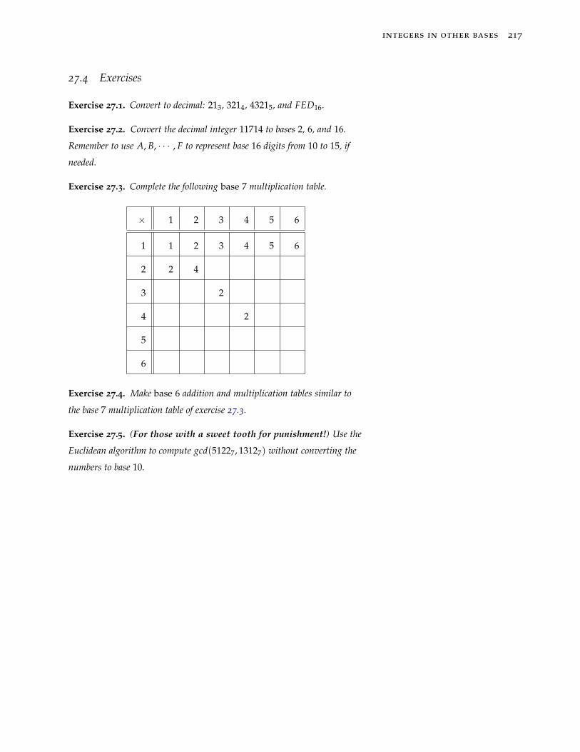
integers in other bases 217
27.4 Exercises
Exercise 27.1. Convert to decimal: 213, 3214, 43215, and FED16.
Exercise 27.2. Convert the decimal integer 11714 to bases 2, 6, and 16.
Remember to use A, B, · · · , F to represent base 16 digits from 10 to 15, if
needed.
Exercise 27.3. Complete the following base 7 multiplication table.
× 1 2 3 4 5 6
1 1 2 3 4 5 6
2 2 4
3 2
4 2
5
6
Exercise 27.4. Make base 6 addition and multiplication tables similar to
the base 7 multiplication table of exercise 27.3.
Exercise 27.5. (For those with a sweet tooth for punishment!) Use the
Euclidean algorithm to compute gcd(51227, 13127) without converting the
numbers to base 10.

28
The Two Fundamental Counting Principles
The next few chapters will deal with the topic of combina-
torics: the art of counting. By counting we mean determining the
number of different ways of arranging objects in certain patterns or
the number of ways of carrying out a sequence of tasks. For example,
suppose we want to count the number of ways of making a bit string
of length two. Such a problem is small enough that the possible ar-
rangements can be counted by brute force. In other words, we can
simply make a list of all the possibilities: 00, 01, 10, 11. So the answer
is four. If the problem were to determine the number of bit strings of
length fifty, the brute force method loses a lot of its appeal. For prob-
lems where brute force counting is not a reasonable alternative, there
are a few principles we can apply to aid in the counting. In fact, there
are just two basic principles on which all counting ultimately rests.
Throughout this chapter, all sets mentioned will be finite sets, and
if A is a set, |A| will denote the number of elements in A.
28.1 The sum rule
The sum rule says that if the sets A and B are disjoint, then
|A ∪ B| = |A|+ |B|.
220 math208: discrete mathematics
Example 28.1. For example, if A = {a, b, c} and B = {j, k, l, m, n}, then
|A| = 3, |B| = 5, and, sure enough,
|A ∪ B| = |{a, b, c, j, k, l, m, n}| = 8 = 3 + 5.
Care must be used when applying the sum principle that the sets �
are disjoint. If A = {a, b, c} and B = {b, c, d}, then |A ∪ B| = 4, and
not 6.
Example 28.2. As another example of the sum principle, if we have a
collection of 3 dogs and 5 cats, then we can select one of the animals in 8
ways.
28.1.1 Counting two independent tasks
The sum principle is often expressed in different language: If we can
do task 1 in m ways and task 2 in n ways, and the tasks are indepen-
dent (meaning that both tasks cannot be done at the same time), then
there are m + n ways to do one of the two tasks. The independence of
the tasks is the analog of the disjointness of the sets in the set version
of the sum rule.
A serious type of error is trying to use the sum rule for tasks that �
are not independent. For instance, suppose we want to know in how
many different ways we can select either a deuce or a six from an ordinary
deck of 52 cards. We could let the first task be the process of selecting a
deuce from the deck. That task can be done in 4 ways since there are
4 deuces in the deck. For the second task, we will take the operation
of selecting a six from the deck. Again, there are 4 ways to accom-
plish that task. Now these tasks are independent since we cannot
simultaneously pick a deuce and a six from the deck. So, according
to the sum rule, there are 4 + 4 = 8 ways of selecting one card from a
deck, and having that card be either a deuce or a six.
Now consider the similar sounding question: In how many ways can
we select either a deuce or a diamond from a deck of 52 cards? We could
let the first task again be the operation of selecting a deuce from
the deck, with 4 ways to carry out that task. And we could let the
second task be the operation of selecting a diamond from the deck,
the two fundamental counting principles 221
with 13 ways to accomplish that. But in this case, the answer to the
question is not 4 + 13 = 17, since these tasks are not independent. It
is possible to select a card that is both a deuce and a diamond. So the
sum rule cannot be used. What is the correct answer? Well, there are
13 diamonds, and there are 3 deuces besides the two of diamonds,
and so there are actually 16 cards in the deck that are either a deuce
or a diamond. That means there are 16 ways to select a card from a
deck and have it turn out to be either a deuce or a diamond.
28.1.2 Extended sum rule
The sum rule can be extended to the case of more than two sets (or
more than two tasks): If A1, A2, A3, · · · , An is a collection of pairwise
disjoint sets, then |A1 ∪ A2 ∪ A3 ∪ · · · ∪ An| = |A1|+ |A2|+ |A3|+· · ·+ |An|. Or, in terms of tasks: If task 1 can be done in k1 ways, and
task 2 in k2, and task 3 in k3 ways, and so on, until task n can be done
in kn ways, and if the tasks are all independent1, then we can do one 1 They must be pairwise independent!
task in k1 + k2 + k3 + · · ·+ kn ways.
Example 28.3. For example, if we own three cars, two bikes, a motorcycle,
four pairs of roller skates, and two scooters, then we can select one of these
modes of transportation in 3 + 2 + 1 + 4 + 2 = 12 ways.
28.1.3 Sum rule and the logical or
The sum rule is related to the logical connective or. That is reasonable
since the sum rule counts the number of elements in the set A ∪ B =
{ x | x ∈ A or x ∈ B }. In terms of tasks, the sum rule counts the
number of ways to do either task 1 or task 2. Generally speaking,
when the word or occurs in a counting problem, the sum rule is the
tool to use. But, verify independence!
28.2 The product rule
The logical connective and is related to the second fundamental
counting principle: the product rule. The product rule says:
|A× B| = |A| · |B|.
222 math208: discrete mathematics
An explanation of this is that A× B consists of all ordered pairs (a, b)
where a ∈ A and b ∈ B. There are |A| choices for a and then |B|choices for b.
28.2.1 Counting two sequential tasks: logical and
In terms of tasks, the product rule says that if task 1 can be done in
m ways and task 2 can be done in n ways after task 1 has been done,
then there are mn ways to do both tasks, the first then the second.
Here the relation with the logical connective and is also obvious. We
need to do task 1 and task 2. Generally speaking, the appearance of
and in a counting problem suggests the product rule will come into
play.
28.2.2 Extended product rule
As with the sum rule, the product rule can be used for situations
with more than two sets or more than two tasks. In terms of sets,
the product rule reads |A1 × A2 × · · · An| = |A1| · |A2| · · · |An|. In
terms of tasks, it reads, if task 1 can be done in k1 ways, and for each
of those ways, task 2 can be done in k2 ways, and for each of those
ways, task 3 can be done in k3 ways, and so on, until for each of those
ways, task n can be done in kn ways, then we can do task 1 followed
by task 2 followed by task 3, etc, followed by task n in k1k2k3 · · · kn
ways. That sounds worse than it really is.
Example 28.4. How many bit strings are there of length five?
Solution. We can think of task 1 as filling in the first (right hand) position,
task 2 as filling in the second position, and so on. We can argue that we
have two ways to do task 1, and then two ways to do task 2, and then two
ways to do task 3, and then two ways to do task 4, and then two ways to do
task 5. So, by the product rule, there are 2 · 2 · 2 · 2 · 2 = 25 = 32 ways to The same reasoning shows that, in
general, there are 2n bit strings of
length n.do all five tasks, and so there are 32 bit strings of length five.
Example 28.5. Suppose we are buying a car with five choices for the ex-
terior color and three choices for the interior color. Then there is a total of
3 · 5 = 15 possible color combinations that we can choose from. The first task
is to select an exterior color, and there are 5 ways to do that. The second task
the two fundamental counting principles 223
is to select an interior color, and there are 3 ways to do that. So the product
rule says there are 15 ways total to do both tasks. Notice that there is no
requirement of independence of tasks when using the product rule. However,
also notice that the number of ways of doing the second task must be the
same no matter what choice is made for doing the first task.
Example 28.6. For another, slightly more complicated, example of the
product rule in action, suppose we wanted to make a two-digit number
using the digits 1, 2, 3, 4, 5, 6, 7, 8, and 9. How many different such two-
digit numbers could we form? Let’s make the first task filling in the left
digit, and the second task filling in the right digit. There are 9 ways to do
the first task. And, no matter how we do the first task, there are 9 ways to do
the second task as well. So, by the product rule, there are 9 · 9 = 81 possible
such two-digit numbers.
Example 28.7. Now, let’s change the problem in example 28.6 a little bit.
Suppose we wanted two-digit numbers made up of those same nine digits,
but we do not want to use a digit more than once in any of the numbers.
In other words, 37 and 91 are OK, but we do not want to count 44 as a
possibility. We can still make the first task filling in the left digit, and the
second task filling in the right digit. And, as before, there are 9 ways to do
the first task. But now, once the first task has been done, there are only 8
ways to do the second task, since the digit used in the first task is no longer No matter in what way the first task
was done, there are always 8 ways to
to the second task in sequence. What if
you chose to pick the second digit first?
available for doing the second task. For instance, if the digit 3 was selected
in the first task, then for the second task, we will have to choose from the
eight digits 1, 2, 4, 5, 6, 7, 8, and 9. So, according to the product rule, there
are 9 · 8 = 72 ways of building such a number.
Example 28.8. Just for fun, here is another way to see the answer in ex-
ample 28.7 is 72. We saw above that there are 81 ways to make a two-digit
number when we allow repeated digits. But there are 9 two digit numbers
that do have repeated digits (namely 11, 22, · · · , 99). That means there must
be 81− 9 = 72 two-digit numbers without repeated digits.
28.2.3 Counting by subtraction: Good = Total − Bad
The trick we used in example 28.8 looks like a new counting princi-
ple, but it is really the sum rule being applied in a tricky way. Here’s
224 math208: discrete mathematics
the idea. Call the set of all the two-digit numbers (not using 0) T, call
the set with no repeated digits N, and call the set with repeated dig-
its R. By the sum rule, |T| = |N|+ |R|, so |N| = |T| − |R|. This is a
very common trick.
Generally, suppose we are interested in counting some arrange-
ments, let’s call them the Good arrangements. But it is not easy for
some reason to count the Good arrangements directly. So, instead, we
count the Total number of arrangements, and subtract the number of
Bad arrangements:
Good = Total − Bad.
Let’s have another example of this trick.
Example 28.9. By a word of length five, we will mean any string of five
letters from the 26 letter alphabet. How many words contain at least one
vowel. The vowels are: a,e,i,o,u.
By the product rule, there is a total of 265 possible words of length five.
The bad words are made up of only the 21 non-vowels. So, by the sum rule,
the number of good words is 265 − 215.
28.3 Using both the sum and product rules
As in example 28.9, most interesting counting problems involve a
combination of both the sum and product rules.
Example 28.10. Suppose we wanted to count the number of different
possible bit strings of length five that start with either three 0’s or with two
1’s. Recall that a bit string is a list of 0’s and 1’s, and the length of the bit
string is the total number of 0’s and 1’s in the list. So, here are some bit
strings that satisfy the stated conditions: 00001, 11111, 11011, and 00010.
On the other hand, the bit strings 00110 and 10101 do not meet the required
condition.
To do this problem, let’s first count the number of good bit strings that
start with three 0’s. In this case, we can think of the construction of such a
bit string as doing five tasks, one after the other, filling in the leftmost bit,
then the next one, then the third, the next, and finally the last bit. There
is only one way to do the first three tasks, since we need to fill in 0’s in the
first three positions. But there are two ways to do the last two tasks, and
the two fundamental counting principles 225
so, according to the product rule there are 1 · 1 · 1 · 2 · 2 = 4 bit strings
of length five starting with three 0’s. Using the same reasoning, there are
1 · 1 · 2 · 2 · 2 = 8 bit strings of length five starting with two 1’s. Now, a
bit string cannot both start with three 0’s and also with two 1’s, (in other
words, starting with three 0’s and starting with two 1’s are independent).
And so, according to the sum rule, there will be a total of 4 + 8 = 12 bit
strings of length five starting with either three 0’s or two 1’s.
Example 28.11. How many words of six letters (repeats OK) contain
exactly one vowel?
Solution. Let’s break the construction of a good word down into a number
of tasks.
Task 1: Select a spot for the vowel: 6 choices.
Task 2: Select a vowel for that spot: 5 choices.
Task 3: Fill first empty spot with a non-vowel: 21 choices
Task 4: Fill next empty spot with a non-vowel: 21 choices
Task 5: Fill next empty spot with a non-vowel: 21 choices
Task 6: Fill next empty spot with a non-vowel: 21 choices
Task 7: Fill last empty spot with a non-vowel: 21 choices
By the product rule, the number of good words is 6 · 5 · 215.
Example 28.12. Count the number of strings on license plates which either
consist of three capital English letters, followed by three digits, or consist of
two digits followed by four capital English letters.
Solution. Let A be the set of strings which consist of three capital English
letters followed by three digits, and B be the set of strings which consist
of two digits followed by four capital English letters. By the product rule
|A| = 263 · 103 since there are 26 capital English letters and 10 digits. Also
by the product rule |B| = 102 · 264. Since A ∩ B = ∅, by the sum rule the
answer is 263 · 103 + 102 · 264.
226 math208: discrete mathematics
28.4 Answer form←→ solution method
In the previous examples we might continue on with the arithmetic.
For instance, in the last, example 28.12, using the distributive law
on our answer to factor out common terms we see |A ∪ B| = 102 ·263(10 + 26) is an equivalent answer. This, in turn, simplifies to
|A ∪ B| = 102 · 263 · 36, and that gives
|A ∪ B| = 100 · 17576 · 36 = 63, 273, 600.
Of all of these answers the most valuable is probably 263 · 103 +
102 · 264, since the form of the answer is indicative of the manner
of solution. We can readily observe that the sum rule was applied to
two disjoint subcases. For each subcase the product rule was applied
to compute the intermediate answer. As a general rule, answers to
counting problems should be left in this uncomputed form.
The next most useful solution is the last one. When we have an
answer of this form we can use it to consider whether or not our
answer makes sense intuitively. For example if we knew that A and
B both were subsets of a set of cardinality 450 and we computed that
|A ∪ B| > 450, this would indicate that we made an error, either in
the logic of our counting, or in arithmetic, or both.
the two fundamental counting principles 227
28.5 Exercises
Exercise 28.1. To meet the science requirement a student must take one of
the following courses: a choice of 5 biology courses, 4 physics courses, or 6
chemistry courses. In how many ways can the one course be selected?
Exercise 28.2. Using the data of problem 1, a student has decided to take
one biology, one physics, and one chemistry course. How many different
such selections are possible?
Exercise 28.3. A code word is either a sequence of three letters followed
by two digits or two letters followed by three digits. (Unless otherwise
indicated, letters will means letters chosen from the usual 26-letter alphabet
and digits are selected from {0, 1, 2, 3, 4, 5, 6, 7, 8, 9}.) How many different
code words are possible?
Exercise 28.4. How many words of length six are there if letters may be
repeated? (Examples: BBBXBB, ABATBC are OK).
Exercise 28.5. How many words of length six are there if letters may not be
repeated? (Examples: BBBBXB, ABATJC are bad but ABXHYR is OK).
Exercise 28.6. A multiple choice test contains 10 questions. There are four
possible answers for each question.
(a) How many ways can a student complete the test if every question must
be answered?
(b) How many ways can a student complete the test if questions can be left
unanswered?
Exercise 28.7. How many binary strings of length less than or equal to
nine are there?
Exercise 28.8. How many eight-letter words contain at least one A?
Exercise 28.9. How many seven-letter words contain at most one A?
Exercise 28.10. How many nine-letter words contain at least two A’s?

29
Permutations and Combinations
By a permutation of a set of objects we mean a listing of the
objects of the set in a specific order. For example, there are six possi-
ble permutations of the set A = {a, b, c}. They are
abc, acb, bac, bca, cab, cba.
The product rule explains why there are six permutation of A:
there are 3 choices for the first letter, once that choice has been made
there are 2 choices for the second letter, and finally that leaves 1
choice for the last letter. So the total number of permutations is 3 · 2 ·1 = 6.
29.1 Permutations
A set with n elements is called an n-set. We have just shown that a
3-set has 6 permutations. The same reasoning shows that an n-set has
n · (n− 1) · (n− 2) · · · 2 · 1 = n! permutations. So the total number
of different ways to arrange a deck of cards is 52!, a number with 68
digits: 80658175170943878571660636856403766975289505440883277824000000000000.
Instead of forming a permutation of all the elements of an n-set,
we might consider the problem of first selecting some of the ele-
ments of the set, say r of them, and then forming a permutation
of just those r elements. In that case we say we have formed an r-
permutation of the n-set. All the possible 2-permutations of the 4-set
230 math208: discrete mathematics
A = {a, b, c, d} are
ab, ac, ad, ba, bc, bd, ca, cb, cd, da, db, dc
Hence, there are twelve 2-permutations of a 4-set.
Notation. In general, P(n, r) denotes the number of different r-permutations The number of 2-permutations of a
4-set is P(4, 2)=12.of an n-set.
The product rule provides a simple formula for P(n, r). There are
n choices for the first element, and once that choice has been made,
there are n − 1 choices for the second element, then n − 2 for the
third, and so on, until finally, there are n − (r − 1) = n − r + 1
choices for the rth element. So P(n, r) = n(n− 1) · ... · (n− r + 1).
That expression can be written more neatly as follows: And, that is the way to remember the
formula:
P(n, r) =n!
(n− r)!.P(n, r) = n(n− 1) · ... · (n− r + 1)
=n(n− 1) · ... · (n− r + 1)(n− r)(n− r− 1) · · · 2 · 1
(n− r)(n− r− 1) · · · 2 · 1 =n!
(n− r)!
Example 29.1. As an example, the number of ways of selecting a president,
vice-president, secretary, and treasurer from a group of 20 people is P(20, 4)
(assuming no person can hold more than one office). If you want the actual
numerical value, it is20!
(20− 4)!= 20 · 19 · 18 · 17 = 116280, but the best
way to write the answer in most cases would be just P(20, 4) =20!16!
, and
skip the numerical computations.
Example 29.2. How many one-to-one functions are there from a 5-set to a
7-set?
While this question doesn’t sound on the surface like a problem of per-
mutations, it really is. Suppose the 5-set is A = {1, 2, 3, 4, 5} and the 7-set
is B = {a, b, c, d, e, f , g}. One example of a one-to-one function from A to
B would be f (1) = a, f (2) = c, f (3) = g, f (4) = b, f (5) = d. But, if
we agree to think of the elements of A listed in their natural order, we could
specify that function more briefly as acgbd. In other words, each one-to-one
function specifies a 5-permutation of B, and, conversely, each 5-permutation
of B specifies a one-to-one function. So the number of one-to-one functions The same reasoning shows there are
P(n, r) one-to-one functions from an
r-set to an n-set.from a 5-set to a 7-set is equal to the number of 5-permutations of a 7-set,
and that is P(7, 5) = 2520.
permutations and combinations 231
Example 29.3. Here are a few easily seen values of P(n, r):
(1) P(n, n) = n!
(2) P(n, 1) = n
(3) P(n, 0) = 1 There is only one 0-permutation, the
one with no symbols!
(4) P(n, r) = 0 if r > n There are no permutations with length
greater than n of n objects.
29.2 Combinations
When forming permutations, the order in which the elements are
listed is important. But there are many cases when we are interested
only in which elements are selected and we do not care about the
order. For example, when playing poker, a hand consists of five cards
dealt from a standard 52-card deck. The order in which the cards
arrive in a hand does not matter, only the final selection of the five
cards is important. When order is not important, the selection is
called a combination rather than a permutation. More carefully, an r-
combination from an n-set is an r-subset of the n-set. In other words
an r-combination of an n-set is an unordered selection of r distinct
elements from the n-set.
Example 29.4. The 2-combinations of the 5-set {a, b, c, d, e} are
{a, b}, {a, c}, {a, d}, {a, e}, {b, c},
{b, d}, {b, e}, {c, d}, {c, e}, {d, e}.
Notation. The number of r-combinations from an n-set is denoted by Example 29.4 shows that
C(5, 2) =(
52
)= 10.C(n, r) or, sometimes,
(nr
).
Example 29.5. Here are a few easily seen values of C(n, r):
(1) C(n, n) = 1
(2) C(n, 1) = n
(3) C(n, 0) = 1 There is only one 0-subset, the empty
set.
(4) C(n, r) = 0 if r > n There are no subsets of an n-set with
size greater than n.
232 math208: discrete mathematics
There is a compact formula for C(n, r) which can be derived using
the product rule in a sort of back-handed way. An r-permutation
of an n-set can be built using a sequence of two tasks. First, select r
elements of the n-set. There are C(n, r) ways to do that task. Next,
arrange those r elements in some specific order. There are r! ways
to do that task. So, according to the product rule, the number of r-
permutations of an n-set will be C(n, r)r!. However, we know that
the number of r-permutations of an n-set are P(n, r). So we may
conclude that P(n, r) = C(n, r)r!, or, rearranging that, we see
C(n, r) =(
nr
)=
P(n, r)r!
=n!
r!(n− r)!
Example 29.6. Suppose we have a club with 20 members. If we want to
select a committee of 4 members, then there are
C(20, 4) =20!
4!(20− 4)!=
20 · 19 · 18 · 174 · 3 · 2 · 1 = 4845
ways to do this since the order of people on the committee doesn’t matter.
Compare this answer with example 29.1 where we counted the
number of possible selections1 for president, vice-president, secretary, 1 P(5, 4) = 20!/16! = 116280 ways
and treasurer from the group of 20. The difference between the two
cases is that the earlier example is a question about permutations (or-
der matters), whereas this example is a question about combinations
(order does not matter).
permutations and combinations 233
29.3 Exercises
Exercise 29.1. In how many ways can the 26 volumes (labeled A through
Z) of the Encyclopedia of PseudoScience be placed on a shelf?
Exercise 29.2. In how many ways can those same 26 volumes be placed
on a shelf if superstitions demand the volumes labeled with vowels must be
adjacent? In how many ways can they be placed on the shelf obeying the
conflicting superstition that volumes labeled with vowels cannot touch each
other?
Exercise 29.3. For those same 26 volumes, how many ways can they be
placed in a two shelf bookcase if volumes A-M go on the top shelf and N-Z
go on the bottom shelf?
Exercise 29.4. In how many ways can seven men and four women sit in a
row if the men must sit together?
Exercise 29.5. 20 players are to be divided into two 10-man teams. In how
many ways can that be done?
Exercise 29.6. A lottery ticket consists of five different integers selected
from 1 to 99. How many different lottery tickets are possible? How many
tickets would you need to buy to have a one-in-a-million chance of winning
by matching all five randomly
Exercise 29.7. A committee of size six is selected from a group of nine
clowns and thirteen lion tamers.
(a) How many different committees are possible?
(b) How many committees are possible if there must be exactly two clowns
on the committee?
(c) How many committees are possible if lion tamers must outnumber
clowns on the committee?

30
The Binomial Theorem and Pascal’s Triangle
The quantity C(n, k) is also written as(
nk
), and called a
binomial coefficient . It gives the number of k-subsets of an n-set, or,
equivalently, it gives the number of ways of selecting k items from n
items.
30.1 Combinatorial proof
Facts involving the binomial coefficients can be proved algebraically,
using the formula(
nk
)=
n!k!(n − k)!
. But often the same facts can
be proved much more neatly by recognizing(
nk
)gives the number
of k-subsets of an n-set. This second sort of proof is called a combina-
torial proof. Here is an example of each type of proof.
Theorem 30.1 (Pascal’s Identity). Let n and k be non-negative integers,
then (n + 1
k
)=
(n
k − 1
)+
(nk
).
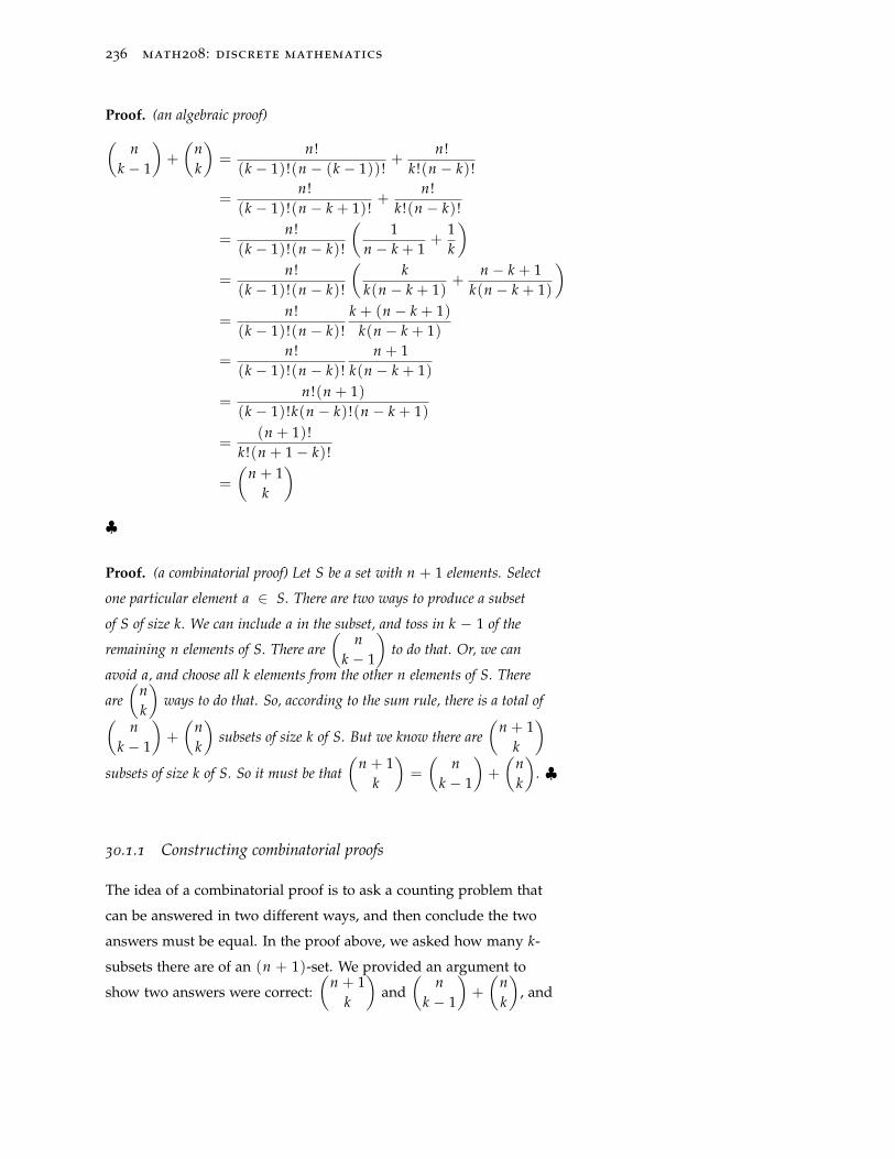
236 math208: discrete mathematics
Proof. (an algebraic proof)(n
k − 1
)+
(nk
)=
n!(k − 1)!(n − (k − 1))!
+n!
k!(n − k)!
=n!
(k − 1)!(n − k + 1)!+
n!k!(n − k)!
=n!
(k − 1)!(n − k)!
(1
n − k + 1+
1k
)=
n!(k − 1)!(n − k)!
(k
k(n − k + 1)+
n − k + 1k(n − k + 1)
)=
n!(k − 1)!(n − k)!
k + (n − k + 1)k(n − k + 1)
=n!
(k − 1)!(n − k)!n + 1
k(n − k + 1)
=n!(n + 1)
(k − 1)!k(n − k)!(n − k + 1)
=(n + 1)!
k!(n + 1 − k)!
=
(n + 1
k
)♣
Proof. (a combinatorial proof) Let S be a set with n + 1 elements. Select
one particular element a ∈ S. There are two ways to produce a subset
of S of size k. We can include a in the subset, and toss in k − 1 of the
remaining n elements of S. There are(
nk − 1
)to do that. Or, we can
avoid a, and choose all k elements from the other n elements of S. There
are(
nk
)ways to do that. So, according to the sum rule, there is a total of(
nk − 1
)+
(nk
)subsets of size k of S. But we know there are
(n + 1
k
)subsets of size k of S. So it must be that
(n + 1
k
)=
(n
k − 1
)+
(nk
). ♣
30.1.1 Constructing combinatorial proofs
The idea of a combinatorial proof is to ask a counting problem that
can be answered in two different ways, and then conclude the two
answers must be equal. In the proof above, we asked how many k-
subsets there are of an (n + 1)-set. We provided an argument to
show two answers were correct:(
n + 1k
)and
(n
k − 1
)+
(nk
), and
the binomial theorem and pascal’s triangle 237
so we could conclude the two answers must be equal:(n + 1
k
)=
(n
k − 1
)+
(nk
).
As in the combinatorial proof of Pascal’s Identity 30.1, such ar-
guments can be much less work, far less tedious, and much more
illuminating, than algebraic proofs. Unfortunately, they can also be
much more difficult to discover since it is necessary to dream up a
good counting problem that will have as answers the two expressions
we are trying to show are equal, and there is no algorithm for coming
up with such a suitable counting problem.
Example 30.2. Give a combinatorial1 proof of(
nk
)=
(n
n− k
). 1 An algebraic proof of this identity is
absolutely trivial:(nk
)=
n!k!(n− k)!
and(n
n− k
)=
n!(n− k)!(n− (n− k))!
=n!
k!(n− k).
Thus, we see that the two expressionsare indeed equal.
Solution. To provide a combinatorial proof, we ask how many ways are
there to grab k elements of an n-set?. One answer of course is(
nk
). But
here is a second way to view the problem. We can select k elements of an
n-set by deciding on n − k elements not to pick. Since there are(
nn− k
)ways to select the n− k not to pick, there must be
(n
n− k
)ways to select k
elements of an n-set. Since the two answers must be equal we conclude that(nk
)=
(n
n− k
). ♣
Example 30.3. Give a combinatorial proof of Vandermonde’s Identity:(n + m
k
)=
(n0
)(mk
)+
(n1
)(m
k− 1
)+
(n2
)(m
k− 2
)+ · · ·+
(nk
)(m0
).
Solution. Consider the set {a1, a2, · · · , an, b1, b2, · · · bm} of n + m ele-
ments. We ask, how may k-subsets does the set have?.
One answer of course is(
n + mk
).
But here’s another way to answer the question:
we can select 0 of the a’s and k of the b’s. There are (n0)(
mk ) ways to do
that.
Or we select 1 of the a’s and k− 1 of the b’s. There are (n1)(
mk−1) ways to
do that.
Or we select 2 of the a’s and k− 2 of the b’s. There are (n2)(
mk−2) ways to
do that.
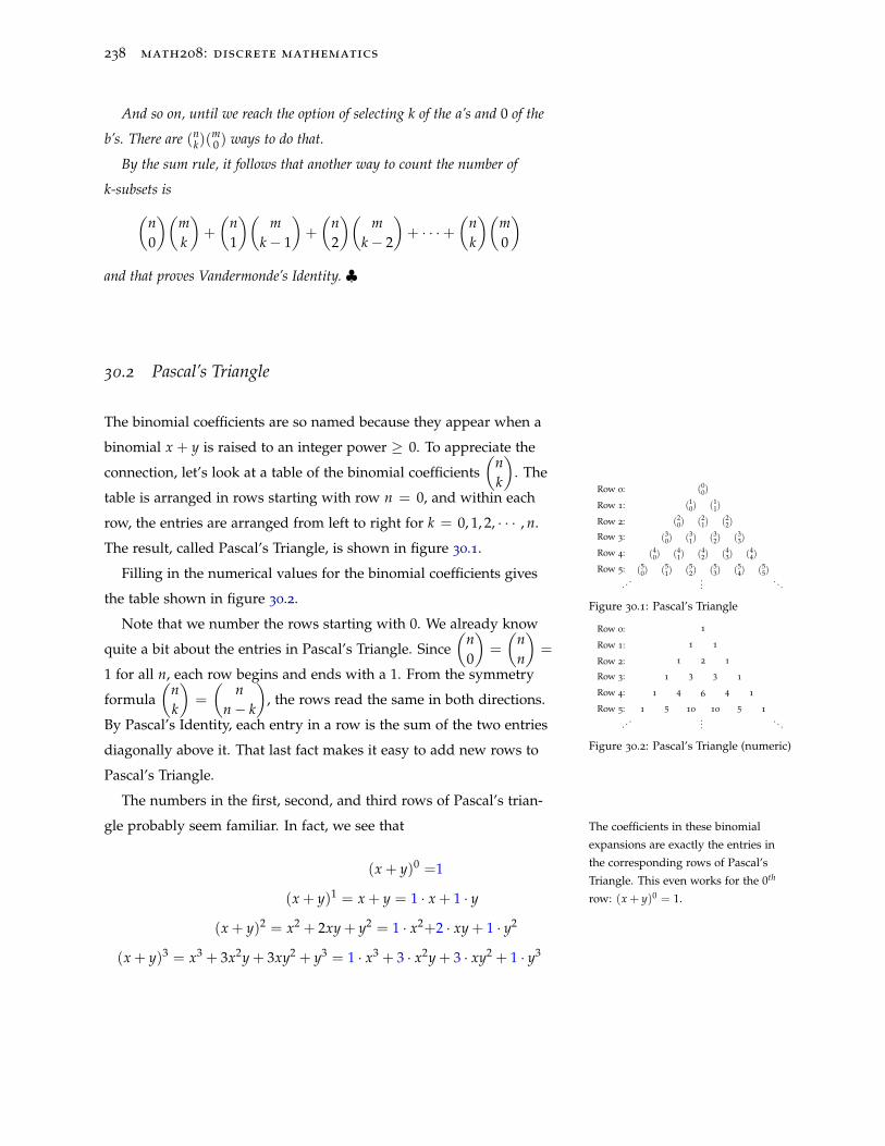
238 math208: discrete mathematics
And so on, until we reach the option of selecting k of the a’s and 0 of the
b’s. There are (nk)(
m0 ) ways to do that.
By the sum rule, it follows that another way to count the number of
k-subsets is(n0
)(mk
)+
(n1
)(m
k− 1
)+
(n2
)(m
k− 2
)+ · · ·+
(nk
)(m0
)and that proves Vandermonde’s Identity. ♣
30.2 Pascal’s Triangle
The binomial coefficients are so named because they appear when a
binomial x + y is raised to an integer power ≥ 0. To appreciate the
connection, let’s look at a table of the binomial coefficients(
nk
). The
table is arranged in rows starting with row n = 0, and within each
row, the entries are arranged from left to right for k = 0, 1, 2, · · · , n.
The result, called Pascal’s Triangle, is shown in figure 30.1.
Row 0: (00)
Row 1: (10) (1
1)
Row 2: (20) (2
1) (22)
Row 3: (30) (3
1) (32) (3
3)
Row 4: (40) (4
1) (42) (4
3) (44)
Row 5: (50) (5
1) (52) (5
3) (54) (5
5)
. . . .... . .
Figure 30.1: Pascal’s Triangle
Filling in the numerical values for the binomial coefficients gives
the table shown in figure 30.2.
Row 0: 1
Row 1: 1 1
Row 2: 1 2 1
Row 3: 1 3 3 1
Row 4: 1 4 6 4 1
Row 5: 1 5 10 10 5 1
. . . .... . .
Figure 30.2: Pascal’s Triangle (numeric)
Note that we number the rows starting with 0. We already know
quite a bit about the entries in Pascal’s Triangle. Since(
n0
)=
(nn
)=
1 for all n, each row begins and ends with a 1. From the symmetry
formula(
nk
)=
(n
n− k
), the rows read the same in both directions.
By Pascal’s Identity, each entry in a row is the sum of the two entries
diagonally above it. That last fact makes it easy to add new rows to
Pascal’s Triangle.
The numbers in the first, second, and third rows of Pascal’s trian-
gle probably seem familiar. In fact, we see that The coefficients in these binomial
expansions are exactly the entries in
the corresponding rows of Pascal’s
Triangle. This even works for the 0th
row: (x + y)0 = 1.
(x + y)0 =1
(x + y)1 = x + y = 1 · x + 1 · y
(x + y)2 = x2 + 2xy + y2 = 1 · x2+2 · xy + 1 · y2
(x + y)3 = x3 + 3x2y + 3xy2 + y3 = 1 · x3 + 3 · x2y + 3 · xy2 + 1 · y3
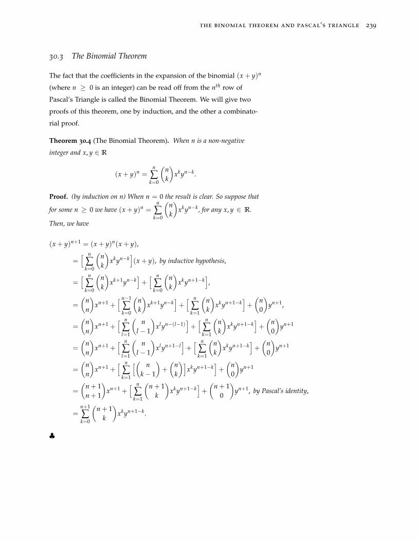
the binomial theorem and pascal’s triangle 239
30.3 The Binomial Theorem
The fact that the coefficients in the expansion of the binomial (x + y)n
(where n ≥ 0 is an integer) can be read off from the nth row of
Pascal’s Triangle is called the Binomial Theorem. We will give two
proofs of this theorem, one by induction, and the other a combinato-
rial proof.
Theorem 30.4 (The Binomial Theorem). When n is a non-negative
integer and x, y ∈ R
(x + y)n =n
∑k=0
(nk
)xkyn−k.
Proof. (by induction on n) When n = 0 the result is clear. So suppose that
for some n ≥ 0 we have (x + y)n =n
∑k=0
(nk
)xkyn−k, for any x, y ∈ R.
Then, we have
(x + y)n+1 = (x + y)n(x + y),
=[ n
∑k=0
(nk
)xkyn−k
](x + y), by inductive hypothesis,
=[ n
∑k=0
(nk
)xk+1yn−k
]+[ n
∑k=0
(nk
)xkyn+1−k
],
=
(nn
)xn+1 +
[ n−1
∑k=0
(nk
)xk+1yn−k
]+[ n
∑k=1
(nk
)xkyn+1−k
]+
(n0
)yn+1,
=
(nn
)xn+1 +
[ n
∑l=1
(n
l − 1
)xlyn−(l−1)
]+[ n
∑k=1
(nk
)xkyn+1−k
]+
(n0
)yn+1
=
(nn
)xn+1 +
[ n
∑l=1
(n
l − 1
)xlyn+1−l
]+[ n
∑k=1
(nk
)xkyn+1−k
]+
(n0
)yn+1
=
(nn
)xn+1 +
[ n
∑k=1
[( nk− 1
)+
(nk
)]xkyn+1−k
]+
(n0
)yn+1
=
(n + 1n + 1
)xn+1 +
[ n
∑k=1
(n + 1
k
)xkyn+1−k
]+
(n + 1
0
)yn+1, by Pascal’s identity,
=n+1
∑k=0
(n + 1
k
)xkyn+1−k.
♣
240 math208: discrete mathematics
Now, let’s look at a combinatorial proof of the Binomial Theorem.
Proof. When the binomial (x + y)n = (x + y)(x + y)(x + y) · · · (x + y)
is expanded, the terms are produced by selecting either the x or the y from
each of the n factors x + y appearing on the right side of the equation. The
number of ways of selecting exactly k x’s from the n available is(
nk
), and
so that will be the coefficient of the term xkyn−k in the expansion. ♣ Isn’t this amazing!
Example 30.5. The coefficient of x7y3 in the expansion of (x + y)10 is(107
)=
10!7!3!
=10 · 9 · 81 · 2 · 3 = 120.
Example 30.6. The coefficient of x7y3 in the expansion of (2x− 3y)10 is(107
)27(−3)3 =
10!7!3!
27(−3)3 = −10 · 9 · 81 · 2 · 3 2733 = −120 · 128 · 27 = −414720.
From the binomial theorem we can derive facts such as
Theorem 30.7. A finite set with n elements has 2n subsets.
Proof. By the sum rule the number of subsets of an n-set is
n
∑k=0
(nk
)=
n
∑k=0
(nk
)1k1n−k.
By the Binomial Theoremn
∑k=0
(nk
)1k1n−k = (1 + 1)n = 2n. ♣
Theorem 30.8. If n ≥ 1, then(n0
)−(
n1
)+
(n2
)− · · ·+ (−1)n
(nn
)= 0.
Proof. By the Binomial Theorem,(n0
)−(
n1
)+
(n2
)− · · ·+ (−1)n
(nn
)= (1− 1)n = 0.
♣
the binomial theorem and pascal’s triangle 241
30.4 Exercises
Exercise 30.1. Determine the sixth row of Pascal’s Triangle.
Exercise 30.2. Determine the coefficient of x3y7 in the expansion of (3x−2y)10.
Exercise 30.3. Give an algebraic proof that(
2n2
)= 2
(n2
)+ n2.
Exercise 30.4. Give a combinatorial proof that(
2n2
)= 2
(n2
)+ n2. Hint:
How many ways are there to select a 2-subset of {a1, a2, · · · , an, b1, b2, · · · bn}?
Exercise 30.5. Give a combinatorial proof that(
3m3
)=
(m3
)+ 2m
(m2
)+ m
(2m2
)+
(2m3
).
Exercise 30.6. Using the same reasoning as in the combinatorial proof of
the Binomial Theorem, determine the coefficient of x4y5z6 in the expansion
of (x + y + z)15.
Exercise 30.7. Show that if p is a prime and 0 < k < p, then p divides(pk
). Hint: When
(pk
)is written out, how many times does p occur as a
factor of the numerator and how many times as a factor of the denominator?

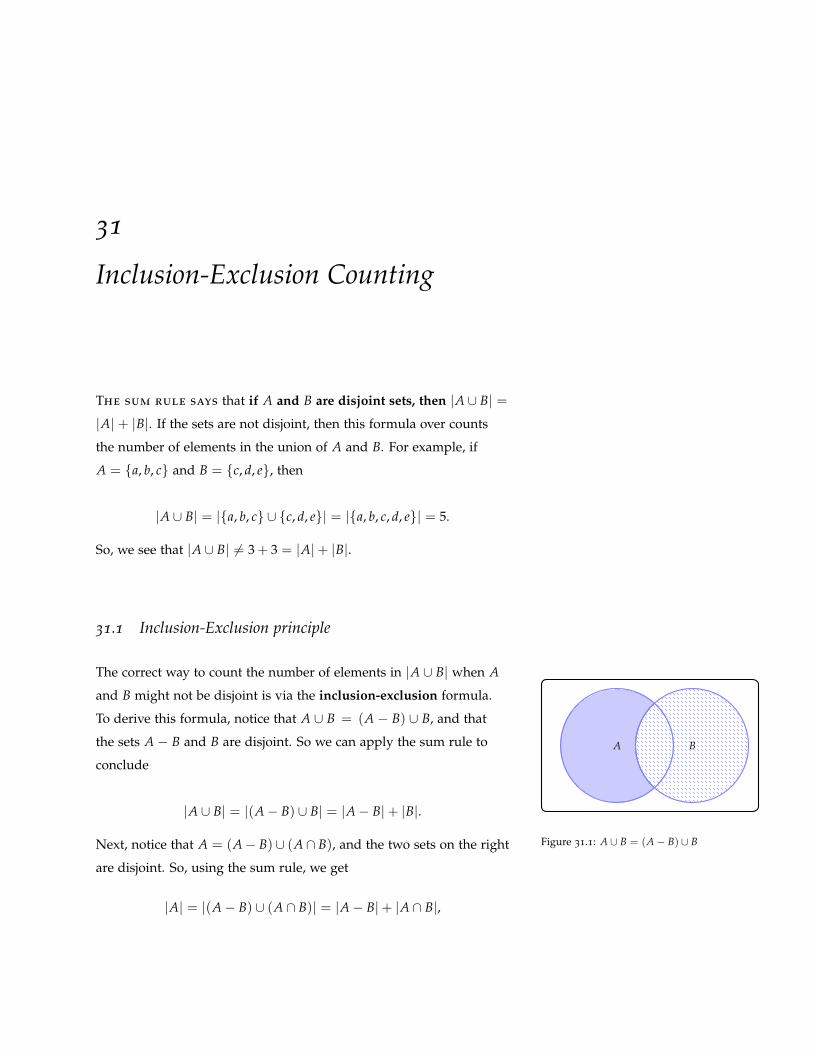
31
Inclusion-Exclusion Counting
The sum rule says that if A and B are disjoint sets, then |A ∪ B| =|A| + |B|. If the sets are not disjoint, then this formula over counts
the number of elements in the union of A and B. For example, if
A = {a, b, c} and B = {c, d, e}, then
|A ∪ B| = |{a, b, c} ∪ {c, d, e}| = |{a, b, c, d, e}| = 5.
So, we see that |A ∪ B| 6= 3 + 3 = |A|+ |B|.
31.1 Inclusion-Exclusion principle
The correct way to count the number of elements in |A ∪ B| when A
and B might not be disjoint is via the inclusion-exclusion formula.
To derive this formula, notice that A ∪ B = (A − B) ∪ B, and that
the sets A − B and B are disjoint. So we can apply the sum rule to
concludeA B
Figure 31.1: A ∪ B = (A− B) ∪ B
|A ∪ B| = |(A− B) ∪ B| = |A− B|+ |B|.
Next, notice that A = (A− B)∪ (A∩ B), and the two sets on the right
are disjoint. So, using the sum rule, we get
|A| = |(A− B) ∪ (A ∩ B)| = |A− B|+ |A ∩ B|,
244 math208: discrete mathematics
which we can rearrange as
|A− B| = |A| − |A ∩ B|.
So, replacing |A − B| by |A| − |A ∩ B| in the formula |A ∪ B| =|(A− B)∪ B| = |A− B|+ |B|, we end up with the inclusion-exclusion
formula:
|A ∪ B| = |A|+ |B| − |A ∩ B|.
In words, to count the number of items in the union of two sets,
include one for everything in the first set, and include one for ev-
erything in the second set, then exclude one for each element in the
overlap of the two sets (since those elements will have been counted
twice).
Example 31.1. How many students are there in a discrete math class if 15
students are computer science majors, 7 are math majors, and 3 are double
majors in math and computer science?
Solution. Let C denote the subset of computer science majors in the class,
and M denote the math majors. Then |C| = 15, |M| = 7 and |C ∩M| = 3.
So by the principle of inclusion-exclusion there are |C|+ |M| − |C ∩M| =15 + 7− 3 = 19 students in the class. ♣
Example 31.2. How many integers between 1 and 1000 are divisible by
either 7 or 11?
Solution. Let S denote the set of integers between 1 and 1000 divisible by
7, and E denote the set of integers between 1 and 1000 divisible by 11. We
need to count the number of integers in S ∪ E. By the principle of inclusion-
exclusion, we have
|S ∪ E| = |S|+ |E| − |S ∩ E| =⌊
10007
⌋+
⌊1000
11
⌋−⌊
100077
⌋= 142 + 90− 12 = 120.
♣
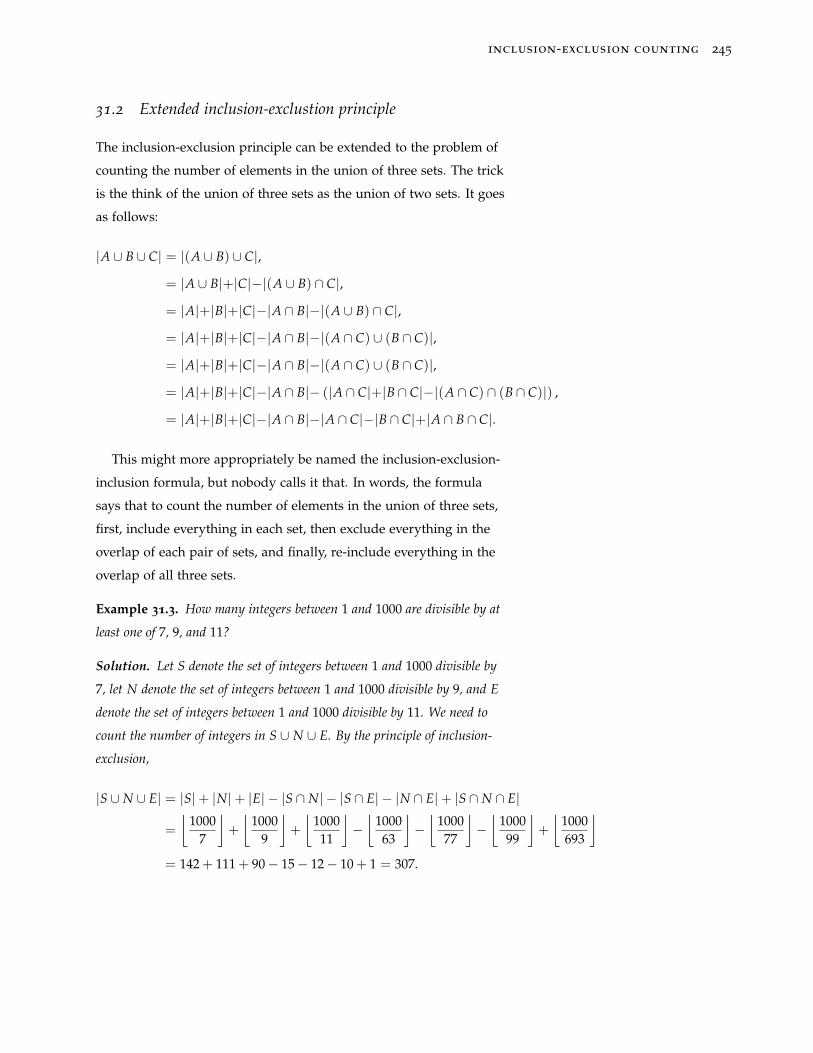
inclusion-exclusion counting 245
31.2 Extended inclusion-exclustion principle
The inclusion-exclusion principle can be extended to the problem of
counting the number of elements in the union of three sets. The trick
is the think of the union of three sets as the union of two sets. It goes
as follows:
|A ∪ B ∪ C| = |(A ∪ B) ∪ C|,
= |A ∪ B|+|C|−|(A ∪ B) ∩ C|,
= |A|+|B|+|C|−|A ∩ B|−|(A ∪ B) ∩ C|,
= |A|+|B|+|C|−|A ∩ B|−|(A ∩ C) ∪ (B ∩ C)|,
= |A|+|B|+|C|−|A ∩ B|−|(A ∩ C) ∪ (B ∩ C)|,
= |A|+|B|+|C|−|A ∩ B|− (|A ∩ C|+|B ∩ C|−|(A ∩ C) ∩ (B ∩ C)|) ,
= |A|+|B|+|C|−|A ∩ B|−|A ∩ C|−|B ∩ C|+|A ∩ B ∩ C|.
This might more appropriately be named the inclusion-exclusion-
inclusion formula, but nobody calls it that. In words, the formula
says that to count the number of elements in the union of three sets,
first, include everything in each set, then exclude everything in the
overlap of each pair of sets, and finally, re-include everything in the
overlap of all three sets.
Example 31.3. How many integers between 1 and 1000 are divisible by at
least one of 7, 9, and 11?
Solution. Let S denote the set of integers between 1 and 1000 divisible by
7, let N denote the set of integers between 1 and 1000 divisible by 9, and E
denote the set of integers between 1 and 1000 divisible by 11. We need to
count the number of integers in S ∪ N ∪ E. By the principle of inclusion-
exclusion,
|S ∪ N ∪ E| = |S|+ |N|+ |E| − |S ∩ N| − |S ∩ E| − |N ∩ E|+ |S ∩ N ∩ E|
=
⌊1000
7
⌋+
⌊1000
9
⌋+
⌊100011
⌋−⌊
100063
⌋−⌊
100077
⌋−⌊
100099
⌋+
⌊1000693
⌋= 142 + 111 + 90− 15− 12− 10 + 1 = 307.
246 math208: discrete mathematics
There are similar inclusion-exclusion formulas for the union of
four, five, six, · · · sets. The formulas can be proved by induction with
the inductive step using the trick we used above to go from two sets
to three. However, there is a much neater way to prove the formula
based on the Binomial Theorem.
Theorem 31.4. Given finite sets A1, A2, ..., An∣∣∣∣∣ n⋃k=1
Ak
∣∣∣∣∣ = n
∑k=1|Ak| − ∑
1≤j<k≤n|Aj ∩ Ak|+ · · ·+ (−1)n−1
∣∣∣∣∣ n⋂k=1
Ak
∣∣∣∣∣ .
Proof. Suppose x ∈ ⋃nk=1 Ak. We need to show that x is counted exactly
once by the right-hand side of the promised formula. Say x ∈ Ai for exactly
p of the sets Ai, where 1 ≤ p ≤ n.
The key to the proof is being able to count the number of intersections in
each summation on the right-hand side of the offered formula that contain
x since we will account for x once for each such term. The number of such
terms in the first sum is n =
(p1
), the number in the second term is
(p2
),
and, in general, the number of terms in the jth sum will be(
pj
)provided
j ≤ p. If j > p then x will not be any of the intersections of j of the sets, and
so will not contribute any more to the right side of the formula.
So the total number of times x is accounted for on the right hand side is(p1
)−(
p2
)− ... + (−1)p−1
(pp
),
= 1−((
p0
)−(
p1
)+
(p2
)− ... + (−1)p
(pp
)),
= 1− (1− 1)p = 1.
Just as we hoped. ♣
Example 31.5. How many students are in a calculus class if 14 are math
majors, 22 are computer science majors, 15 are engineering majors, and 13
are chemistry majors, if 5 students are double majoring in math and com-
puter science, 3 students are double majoring in chemistry and engineering,
10 are double majoring in computer science and engineering, 4 are double
majoring in chemistry and computer science, none are double majoring in
math and engineering and none are double majoring in math and chemistry,
and no student has more than two majors?
inclusion-exclusion counting 247
Solution. Let A1 denote the math majors, A2 denote the computer science
majors, A3 denote the engineering majors, and A4 the chemistry majors.
Then the information given is
|A1| = 14, |A2| = 22, |A3| = 15, |A4| = 13,
|A1 ∩ A2| = 5, |A1 ∩ A3| = 0, |A1 ∩ A4| = 0,
|A2 ∩ A3| = 10, |A2 ∩ A4| = 4, |A3 ∩ A4| = 3,
|A1 ∩ A2 ∩ A3| = 0, |A1 ∩ A2 ∩ A4| = 0,
|A1 ∩ A3 ∩ A4| = 0, |A2 ∩ A3 ∩ A4| = 0,
and
|A1 ∩ A2 ∩ A3 ∩ A4| = 0.
So, by inclusion-exclusion, the number of students in the class is
14 + 22 + 15 + 13− 5− 10− 4− 3 = 42.
Example 31.6. How many ternary strings (using 0’s, 1’s and 2’s) of length
8 either start with a 1, end with two 0’s or have 4th and 5th positions 12,
respectively?
Solution. Let A1 denote the set of ternary strings of length 8 which start
with a 1, A2 denote the set of ternary strings of length 8 which end with two
0’s, and A3 denote the set of ternary strings of length 8 which have 4th and
5th positions 12. By inclusion-exclusion, the answer is 37 + 36 + 36 − 35 −35 − 34 + 33.
31.3 Inclusion-exclusion with the Good=Total-Bad trick
The inclusion-exclusion formula is often used along with the Good=Total-
Bad trick.
Example 31.7. How many integers between 1 and 1000 are divisible by
none of 7, 9, and 11?
Solution. There are 1000 numbers between 1 and 1000 (assuming 1 and
1000 are included). As counted before, there are 307 of those that are divisi-
248 math208: discrete mathematics
ble by at least one of 7, 9, and 11. That means there are 1000− 307 = 693
that are divisible by none of 7, 9, or 11.
inclusion-exclusion counting 249
31.4 Exercises
Exercise 31.1. At a certain college no student is allowed more than two
majors. How many students are in the college if there are 70 math majors,
160 chemistry majors, 230 biology majors, 56 geology majors, 24 physics
majors, 35 anthropology majors, 12 double math-physics majors, 10 double
math-chemistry majors, 4 double biology-math majors, 53 double biology-
chemistry majors, 5 double biology-anthropology majors, and no other dou-
ble majors?
Exercise 31.2. How many bit strings of length 15 start with the string
1111, end with the string 1000 or have 4th through 7th bits 1010?
Exercise 31.3. How many positive integers between 1000 and 9999 inclu-
sive are not divisible by any of 4, 10 or 25 (careful!)?
Exercise 31.4. How many permutations of the digits 1, 2, 3, 4, 5, have at
least one digit in its own spot? In other words, a 1 in the first spot, or a 2 in
the second, etc. For example, 35241 is OK since it has a 4 in the fourth spot,
and 14235 is OK, since it has a 1 in the first spot (and also a 5 in the fifth
spot). But 31452 is no good. Hint: Let A1 be the set of permutations that
have 1 in the first spot, let A2 be the set of permutations that 2 in the second
spot, and so on.
Exercise 31.5. How many permutations of the digits 1, 2, 3, 4, 5 have no
digit in its own spot?

32
The Pigeonhole Principle
The pigeonhole principle, like the sum and product rules, is an-
other one of those absolutely obvious counting facts. The statement
is simple: If n + 1 objects are divided into n piles (some piles can be
empty), then at least one pile must have two or more objects in it. Or,
more colorfully, if n + 1 pigeons land in n pigeonholes, then at least
one pigeonhole has two or more pigeons. What could be more obvi-
ous? The pigeonhole principle is used to show that no matter how a
certain task is carried out, some specific result must always happen.
As a simple example, suppose we have a drawer containing ten
identical black socks and ten identical white socks. How many socks
do we need to select to be sure we have a matching pair? The answer
is three. Think of the pigeonholes as the colors black and white, and
as each sock is selected put it in the pigeonhole of its color. After we
have placed the third sock, one of the two pigeonholes must have at
least two socks in it, and we will have a matching pair. Of course, we
may have been lucky and had a pair after picking the second sock,
but the pigeonhole principle guarantees that with the third sock we
will have a pair.
As another example, suppose license plates are made consisting of
four digits followed by two letters. Are there enough license plates
for a state with seven million cars? No, since there are only 104 ·262 = 6760000 possible license plates, and so, by the pigeonhole
principle, at least two of the seven million plates assigned would
have to be the same.
252 math208: discrete mathematics
32.1 General pigeonhole principle
A slightly fancier version of the pigeonhole principle says that if N
objects are distributed in k piles, then there must be a least one pile
with⌈
Nk
⌉objects in it.
That formula looks impressive, but actually is easy to understand.
For example, if there are 52 people in a room, we can be absolutely
certain that there are at least eight born on the same day of the week.
Think of it this way: with 49 people, it would be possible to have
seven born on each of the seven days of the week. But when the Avoidance principle: how long can we
go before our hand is forced?50th one is reached, it must boost one day up to an eighth person.
That is really about all there is to it. The general proof of the fancy
pigeonhole principle uses this same sort of reasoning. It is a proof by
contradiction, and goes as follows:
Theorem 32.1 (Pigeonhole Principle). If N objects are distributed in k
piles, then there must be a least one pile with⌈
Nk
⌉objects in it.
Proof. Suppose we have N objects distributed in k piles, and suppose
that every pile has fewer than⌈
Nk
⌉objects in it. That means that the piles
each contain⌈
Nk
⌉− 1 or fewer objects. We will use the fact that
⌈Nk
⌉<
Nk + 1 to complete the proof. The total number of object will be at most
k(⌈
Nk
⌉− 1)< k
((Nk + 1
)− 1)= N. That is a contradiction since we
know there is a total of N objects in the k piles. ♣
32.2 Examples
Even though the pigeonhole principle sounds very simple, clever
applications of it can produce totally unexpected results.
Example 32.2. Five misanthropes move to a perfectly square deserted island
that measures two kilometers on a side. Of course, being misanthropes, they
want to live as far from each other as possible. Show that, no matter where
they build on the island, some two will be no more than√
2 kilometers of
each other.
Solution. Divide the island into four one kilometer by one kilometer squares
by drawing lines joining the midpoints of opposite sides. Since there are five
the pigeonhole principle 253
people and four squares, the pigeonhole principle guarantees there will be
two people living in one of those four squares. But people in one of those
squares cannot be further apart than the length of the diagonal of the square
which is, according to Pythagoras,√
2. ♣
Example 32.3. For any positive integer n, there is a positive multiple of
n made up of a number of 1’s followed by a number of 0’s. For example, for
n = 1084, we see 1084 · 1025 = 1111100.
Solution. Consider the n + 1 integers 1, 11, 111, · · · , 11 · · · 1, where the
last one consists of 1 repeated n + 1 times. Some two of these must be the
same modulo n, and so n will divide the difference of some two of them. But
the difference of two of those numbers is of the required type. ♣
Example 32.4. Bill has 20 days to prepare his tiddledywinks title defense.
He has decided to practice at least one hour every day. But, to avoid burn-
out, he will not practice more than a total of 30 hours. Show there is a se-
quence of consecutive days during which he practices exactly 9 hours.
Solution. For j = 1, 2, · · · 20, let tj = the total number of hours Bill
practices up to and including day j. Since he practices at least one hour
every day, and the total number of hours is no more than 30, we see
0 < t1 < t2 < · · · < t20 ≤ 30.
Adding 9 to each term we get
9 < t1 + 9 < t2 + 9 < · · · < t20 + 9 ≤ 39.
So we have 40 integers t1, t2, · · · , t20, t1 + 9, · · · t20 + 9, all between
1 and 39. By the pigeonhole principle, some two must be equal, and the
only way that can happen is for ti = tj + 9 for some i and j. It follows
that ti − tj = 9, and since the difference ti − tj is the the total number of
hours Bill practiced from day j + 1 to day i, that shows there is a sequence of
consecutive days during which he practiced exactly 9 hours. ♣

254 math208: discrete mathematics
32.3 Exercises
Exercise 32.1. Show that in any group of eight people, at least two were
born on the same day of the week.
Exercise 32.2. Show that in any group of 100 people, at least 15 were born
on the same day of the week.
Exercise 32.3. How many cards must be selected from a deck to be sure that
at least six of the selected cards have the same suit?
Exercise 32.4. Show that in any set of n positive integers, where n ≥ 2,
there must be a pair with a difference that is a multiple of n− 1.
Exercise 32.5. Al has 75 days to master discrete mathematics. He decides
to study at least one hour every day, but no more than a total of 125 hours.
Show there must be a sequence of consecutive days during which he studies
exactly 24 hours.
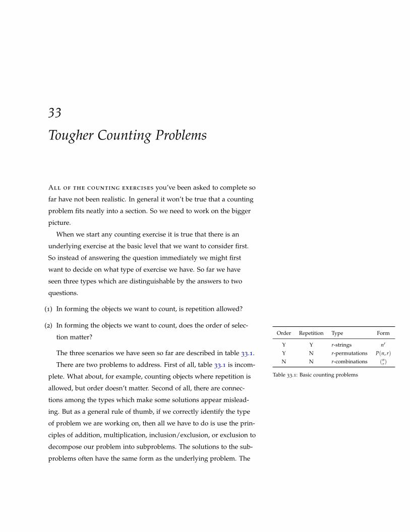
33
Tougher Counting Problems
All of the counting exercises you’ve been asked to complete so
far have not been realistic. In general it won’t be true that a counting
problem fits neatly into a section. So we need to work on the bigger
picture.
When we start any counting exercise it is true that there is an
underlying exercise at the basic level that we want to consider first.
So instead of answering the question immediately we might first
want to decide on what type of exercise we have. So far we have
seen three types which are distinguishable by the answers to two
questions.
(1) In forming the objects we want to count, is repetition allowed?
(2) In forming the objects we want to count, does the order of selec-
tion matter?
The three scenarios we have seen so far are described in table 33.1.
Order Repetition Type Form
Y Y r-strings nr
Y N r-permutations P(n, r)
N N r-combinations (nr)
Table 33.1: Basic counting problems
There are two problems to address. First of all, table 33.1 is incom-
plete. What about, for example, counting objects where repetition is
allowed, but order doesn’t matter. Second of all, there are connec-
tions among the types which make some solutions appear mislead-
ing. But as a general rule of thumb, if we correctly identify the type
of problem we are working on, then all we have to do is use the prin-
ciples of addition, multiplication, inclusion/exclusion, or exclusion to
decompose our problem into subproblems. The solutions to the sub-
problems often have the same form as the underlying problem. The
256 math208: discrete mathematics
principles we employed direct us on how the sub-solutions should be
recombined to give the final answer.
Example 33.1. As an example of the second problem, if we ask how many
binary strings of length 10 contain exactly three 1’s, then the underlying
problem is an r-string problem. But in this case the answer is(
103
). Of
course this is really(
103
)1317 from the binomial theorem. In this case
the part of the answer which looks like nr is suppressed since it’s trivial.
To see the difference we might ask how many ternary strings of length 10
contain exactly three 1’s. Now the answer is(
103
)1327, since we choose the
three positions for the 1’s to go in, and then fill in each of the 7 remaining
positions with a 0 or a 2.
33.1 The Basic Donut Shop Problem
To begin to address the first problem we introduce If you get to the
donut shop before the cops get there, you will find that they have a
nice variety of donuts. You might want to order several dozen. They
will put your order in a box. You don’t particularly care what order
the donuts are put into the box. You do usually want more than one
of several types. The number of ways for you to complete your order
is therefore a counting problem where order doesn’t matter, and
repetition is allowed.
In order to answer the question of how many ways you can com-
plete your order, we first recast the problem mathematically. From
among n types of objects we want to select r objects. If xi denotes the
number of objects of the ith type selected, we have 0 ≤ xi, (since we
cannot choose a negative number of chocolate donouts), also xi ∈ Z,
(since we cannot select fractional parts of donuts). So, the different
ways to order are in one-to-one correspondence with the solutions to
x1 + x2 + ... + xn = r, with xi ≥ 0, xi ∈ Z, for i− 1, 2, . . . , n.
Next, in order to compute the number of solutions in non-negative
integers to x1 + x2 + ... + xn = r, we model each solution as a string
(possibly empty) of x1 1’s followed by a +, then a string of x2 1’s
tougher counting problems 257
followed by a +, ... then a string of xn−1 1’s followed by a +, then a
string of xn 1’s. So for example, if x1 = 2, x2 = 0, x3 = 1, x4 = 3 is a
solution to x1 + x2 + x3 + x4 = 6 the string we get is 11 ++1 + 111.
Finally, we see that the total number of solutions in non-negative
integers to x1 + ... + xn = r, is the number of binary strings of length
r + n− 1 with exactly r 1’s and (n− 1) +’s. From the remark above,
the number of ways to select r donuts from n different types is(n + r− 1
r
).
33.2 The More Realistic Donut Shop Problem
The basic donut shop problem is not very realistic in two ways. First
it is common that some of your order will be determined by other
people. You might for example canvas the people in your office be-
fore you go to see if there is anything you can pick up for them. So
whereas you want to order r donuts, you might have been asked to
pick up a certain number of various types.
Now suppose that we know that we want to select r donuts from
among n types so that at least ai(ai ≥ 0) donuts of type i are selected.
In terms of our equation, we have x1 + x2 + ...+ xn = r, where ai ≤ xi,
and xi ∈ Z. If we set yi = xi − ai for i = 1, ..., n, and a =n
∑i=1
ai, then
0 ≤ yi, yi ∈ Z and
n
∑i=1
yi =n
∑i=1
(xi − ai) =
[n
∑i=1
xi
]−[
n
∑i=1
ai
]= r− a.
So, the number of ways to complete our order is(
n + (r− a)− 1(r− a)
). First ask for the donuts your colleagues
wanted (total of a), then randomly get
the rest (r− a).Still, we qualified the donut shop problem by supposing that we
arrived before the cops did.
33.3 The Real Donut Shop Problem
If we arrive at the donut shop after canvassing our friends, we want
to select r donuts from among n types. The problem is that there
are probably only a few left of each type. This may place an upper
258 math208: discrete mathematics
limit on how often we can select a particular type. So now we wish to
count solutions to
x1 + x2 + ... + xn = r, with ai ≤ xi ≤ bi, xi ∈ Z.
We proceed by replacing r by s = r − a, where a is the sum of
lower bounds. We also replace bi by ci = bi − ai for i = 1, ..., n. So
we want to find the number of solutions to 0 ≤ yi ≤ ci, yi ∈ Z, and
y1 + y2 + ... + yn = s. There are several ways to proceed. We choose
inclusion/exclusion. Let us set U to be all solutions in non-negative
integers to y1 + ...+ yn = s. Next let Ai denote those solutions in non-
negative integers to y1 + ... + yn = r, where ci < yi. Then we want
to compute |A1 ∩ A2 ∩ A3 ∩ ... ∩ An|, which we can do by general
inclusion/exclusion, and the ideas from the more realistic donut shop
problem.
Example 33.2. Let us count the number of solutions to
x1 + x2 + x3 + x4 = 34,
where 0 ≤ x1 ≤ 4, 0 ≤ x2 ≤ 5, 0 ≤ x3 ≤ 8 and 0 ≤ x4 ≤ 40.
As discussed above, we have c1 = 4, c2 = 5, c3 = 8, and c4 = 40. Hence,
we see that
|U | =(
34 + 4− 134
).
Now, Ai will denote the solutions in non-negative integers to
x1 + x2 + x3 + x4 = 34, with xi > ci, for i = 1, 2, 3, 4.
Next, realize that A4 = ∅, so we have
A4 = U and A1 ∩ A2 ∩ A3 ∩ A4 = A1 ∩ A2 ∩ A3.
Now, to compute A1, we must first rephrase x1 > 4 as a non-strict inequal-
ity, i.e. 5 ≤ x1. So, it follows that
|A1| =(
29 + 4− 129
).
tougher counting problems 259
Similarly, we have
|A2‖ =(
28 + 4− 128
), and |A3| =
(25 + 4− 1
25
).
Next, we observe that A1 ∩ A2 represents the set of all solutions in non-
negative integers to
x1 + x2 + x3 + x4 = 34 with 5 ≤ x1 and 6 ≤ x2.
So, we have
|A1 ∩ A2| =(
23 + 4− 123
).
Also, we find that
|A1 ∩ A3| =(
20 + 4− 120
)and |A2 ∩ A3| =
(19 + 4− 1
19
).
Finally, we see that
|A1 ∩ A2 ∩ A3| =(
14 + 4− 114
).
Hence, the final answer is1 1 We leave the answer in this form forclarity. The numerical value is notilluminating.(
34 + 4− 134
)−(
29 + 4− 129
)−(
28 + 4− 128
)−(
25 + 4− 125
)+
(23 + 4− 1
23
)+
(20 + 4− 1
20
)+
(19 + 4− 1
19
)−(
14 + 4− 114
).
We can now solve general counting exercises where order is unim-
portant and repetition is restricted somewhere between no repetition,
and full repetition.
33.4 Problems with order and some repetition
To complete the picture we should be able to also solve counting
exercises where order is important and repetition is partial. This is
somewhat easier. It suffices to consider the subcases in example 33.3.
Example 33.3. Let us take as initial problem the number of quaternary
strings of length 15. There are 415 of these.
Now, if we ask how many contain exactly two 0’s, the answer is(
152
)313.
260 math208: discrete mathematics
If we ask how many contain exactly two 0’s and four 1’s, the answer is(152
)(134
)29.
And, if we ask how many contain exactly two 0’s, four 1’s and five 2’s,
the answer is (152
)(134
)(95
)(44
)=
15!2! · 4! · 5! · 4!
.
So, in fact many types of counting are related by what we call the
multinomial theorem.
Theorem 33.4. When r is a non-negative integer and x1, x2, ..., xn ∈ R, we
have
(x1 + x2 + ... + xn)r = ∑
e1+e2+...+en=r0≤ei
(r
e1, e2, ..., en
)xe1
1 xe22 ...xen
n ,
where(
re1, e2, ...en
)=
r!e1!e2!...en!
.
33.5 The six fundamental counting problems
To recap, when we have a counting exercise, we should first ask
whether order is important and then ask whether repetition is al-
lowed. This will get us into the right ballpark as far as the form of
the solution. We must use basic counting principles to decompose
the exercise into sub-problems. Solve the sub-problems, and put
the pieces back together. Solutions to sub-problems usually take the
same form as the underlying problem, though they may be related to
it via the multinomial theorem. Table 33.2 synopsizes our six funda-
mental cases.
Order Repetition Form
Y Y nr
Y N P(n, r)
N Y(
r + n− 1r
)N N
(nr
)Y some
(r
k1, k2, ..., kn
)N some
(r + n− 1
r
)w/ I-E
Table 33.2: Six counting problems
tougher counting problems 261
33.6 Exercises
Exercise 33.1. How many quaternary strings of length n are there (a
quaternary string uses 0’s, 1’s, 2’s, and 3’s)?
Exercise 33.2. How many quaternary strings of length less than or equal to
7 are there?
Exercise 33.3. How many solutions in integers are there to x1 + x2 +
x3 + x4 + x5 + x6 + x7 = 54, where 3 ≤ x1, 4 ≤ x2, 5 ≤ x3, and
6 < x4, x5, x6, x7?
Exercise 33.4. How many ternary strings of length n start 0101 and end 212?
Exercise 33.5. A doughnut shop has 8 kinds of doughnuts: chocolate,
glazed, sugar, cherry, strawberry, vanilla, caramel, and jalapeno. How many
ways are there to order three dozen doughnuts, if at most 4 are jalapeno, at
most 6 are cherry, and at most 8 are strawberry, but there are no restrictions
on the other varieties?
Exercise 33.6. How many strings of twelve lowercase English letters are there
(a) which start with the letter x, if letters may be repeated?
(b) which contain the letter x at least once, if letters can be repeated?
(c) which contain each of the letters x and y at least once, if letters can be
repeated?
(d) which contain at least one vowel, where letters may not be repeated?
Exercise 33.7. How many bit strings of length 19 either begin “0101", or
have 4th, 5th and 6th digits “101", or end “1010"?
Exercise 33.8. How many pentary strings of length 15 consist of three 0’s,
four 1’s, three 2’s, four 3’s and one 4?
Exercise 33.9. How many ternary strings of length 9 have
(a) exactly four 1’s?
(b) at least three 0’s?
(c) at most three 1’s?
262 math208: discrete mathematics
Exercise 33.10. Seven lecturers and fourteen professors are on the faculty of
a math department.
(a) How many ways are there to form a committee with seven members
which contains more lecturers than professors?
(b) How many ways are there to form a committee with seven members
where the professors outnumber the lecturers on the committee by at least
a two-to-one margin?
(c) How many ways are there to form a committee consisting of at least five
lecturers?
Exercise 33.11. How many ways are there to seat six people at a circular
table where two seatings are considered equivalent if one can be obtained
from the other by rotating the table?
Exercise 33.12. Prove that a set with n ≥ 1 elements has the same number
of subsets with an even number of elements, as subsets with an odd number
of elements.
34
Counting Using Recurrence Relations
It is not always convenient to use the methods of earlier chap-
ters to solve counting problems. Another technique for finding the
solution to a counting problem is recursive counting. The method
will be illustrated with several examples.
34.1 Recursive counting method
Example 34.1. Recall that a bit string is a list of 0’s and 1’s, and the length
of a bit string is the total number of 0’s and 1’s in the string. For example,
10111 is a bit string of length five, and 000100 is a bit string of length six.
The problem of counting the number of bit strings of length n is duck soup.
There are two choices for each bit, and so, applying the product rule, there
are 2n such strings. However, consider the problem of counting the number
of bit strings of length n with no adjacent 0’s.
Let’s use an to denote the number of bit strings of length n with no adja-
cent 0’s. Here are a few sample cases for small values of n.
n=0: Just one good bit string of length zero, and that is λ, the empty bit string.
So a0 = 1.
n=1: There are two good bit strings of length one. Namely 0 and 1. So a1 = 2.
n=2: There are three good bit strings of length two. Namely, 01, 10 and 11.
(Of course, 00 is a bad bit string.) That means a2 = 3.
n=3: Things start to get confusing now. But here is the list of good bit strings
of length three: 010, 011, 101, 110, and 111. So a3 = 5.
264 math208: discrete mathematics
n=4: A little scratch work produces the good bit strings 0101, 0111, 1011,
1101, 1111, 0110, 1010, and 1110, for a total of eight. That means a4 =
8.
We can do a few more, but it is hard to see a formula for an like the 2n
formula that gives the total number of all bit strings of length n. Even
though a formula for an is difficult to spot, there is a pattern to the list of
values for an which looks like the Fibonacci sequence pattern. In fact, the
list so far looks like 1, 2, 3, 5, 8, and if a few more are worked out by brute
force, it turns out the list continues 13, 21, 34. So, it certainly seems that
the solution to the counting problem can be expressed recursively as a0 = 1,
a1 = 2, and for n ≥ 2, an = an−1 + an−2. If this guess is really correct,
then we can quickly compute the number of good bit strings of length n. We
just calculate a0, a1, a2, etc., until we reach the an we are interested in.
Such a recursive solution to counting problems is certainly less
satisfactory than a simple formula, but some counting problems
are so messy that a simple formula might not be possible, and the
recursive solution is better than nothing in such a case.
There is one problem with the recursive solution offered in ex-
ample 34.1. We said that it seems that the solution to the counting
problem can be expressed recursively as a0 = 1, a1 = 2, and for
n ≥ 2, an = an−1 + an−2. That it seems that is not an acceptable justifi-
cation of the formula. After all, we are basing that guess on just eight
or ten values of the infinite sequence an, and it is certainly possible
that those values happen to follow the pattern we’ve guessed simply
by accident. Maybe the true pattern is much more complicated, and
we have been tricked by the small number of cases we have consid-
ered. It is necessary to show that the guessed pattern is correct by
supplying a logical argument.
Our argument would begin by checking the initial conditions we
offered. In other words, we would verify by hand that a0 = 1 and
a1 = 2. This serves as a basis for the verification of the recursive
formula. Now what we want to do is assume that we have already
calculated all the values a0, a1, · · · , ak for some k ≥ 1, and show
that ak+1 must equal ak + ak−1. It is very important to understand
that we do not want to compute the value of ak+1. We only want to prove
counting using recurrence relations 265
that ak+1 = ak + ak−1. The major error made doing these types of
problems is attempting to compute the specific value of ak+1. Don’t
fall for that trap! After all, if it were possible to actually compute the
specific value of ak+1, then we could find a formula for an in general,
and we wouldn’t have to be seeking a recursive relation at all.
Here is how the argument would go in the bit string example.
Suppose we have lists of the good bit strings of lengths 0, 1, · · · , k.
Here is how to make a list of all the good bit strings of length k + 1.
First, take any good bit string of length k and add a 1 on the right
hand end. The result must be a good bit string of length k + 1 (since
we added a 1 to the end, and the original bit string didn’t have two
consecutive 0’s, the new bit string cannot have two consecutive 0’s
either). In that way we form some good bit strings of length k +
1. In fact, we have built exactly ak good bit strings of length k +
1. But wait, there’s more! (as they say in those simple-minded TV
ads). Another way to build a good bit string of length k + 1 is to
take a good bit string of length k − 1 and add 10 to the right end.
Clearly these will also be good bit strings of length k + 1. And these
all end with a 0, so they are all new ones, and not ones we built in
the previous step. How many are there of this type? One for each
of the good bit strings of length k − 1, or a total of ak−1. Thus, so
far we have built ak + ak−1 good bit strings of length k + 1. Now we
will show that in fact we have a complete list of all good bit string of
length k + 1, and that will complete the proof that ak+1 = ak + ak−1.
But before driving that last nail into the coffin, let’s look at the steps
outlined above for the case k + 1 = 4.
The previous paragraph essentially provides an algorithm for
building good bit strings of length k + 1 from good bits strings of
lengths k and k − 1. The algorithm instructs us to add 1 to the right
end of all the good bit strings of length k and 10 to the right of all the
good bit strings of length k− 1. Applying the algorithm for the case
k + 1 = 4, gives the following list, where the added bits are put in
parentheses to make them stand out. 010(1), 011(1), 101(1), 110(1),
111(1), 01(10), 10(10), and 11(10).
There remains one detail to iron out. It is clear that the algorithm
266 math208: discrete mathematics
will produce good bit strings of length k + 1. But, does it produce
every good bit string of length k + 1? If it does not, then the recursive
relation we are offering for the solution to the counting problem will
eventually begin to produce answers that are too small, and we will
undercount the number of good bit strings. To see that we do count
all good bit strings of length k + 1, consider any particular good bit
string of length k + 1, call it s for short, and look at the right most
bit of s. There are two possibilities for that bit. It could be a 1. If that
is so, then when the 1 is removed the remaining bit string is a good
of length k (it can’t have two adjacent 0’s since s doesn’t have two
adjacent 0’s). That means the bit string s is produced by adding a 1
to the right end of a good bit string of length k, and so s is produced
by the first step in the algorithm. The other option for s is that the
right most bit is a 0. But then the second bit in from the right must be
a 1, since s is a good bit string, so it doesn’t have adjacent 0’s. So the
last two bits on the right of s are 10. If those two bits are removed,
there remains a good bit string of length k− 1. Thus s is produced by
adding 10 to the right end of a good bit string of length k− 1, and so
s is produced by the second case in the algorithm.
In a nutshell, we have shown our algorithm produces ak + ak−1
good bit strings of length k + 1, and that the algorithm does not
miss any good bit strings of length k + 1. Thus we have proved that
ak+1 = ak + ak−1 for all k ≥ 2.
Example 34.1 was explained in excruciating detail. Normally, the
verifications will be much more briefly presented. It takes a while to
get used to recursive counting, but once the light goes on, the beauty
and simplicity of the method will become apparent.
34.2 Examples
Example 34.2. This example is a little silly since it is very easy to write
down a formula to solve the counting problem. But the point of the example
is not find the solution to the problem but rather to exhibit recursive count-
ing in action. The problem is to compute the total number of individual
squares on an n× n checkerboard. If we let the total number of squares be
counting using recurrence relations 267
denoted by sn, then obviously sn = n2. For example, an ordinary checker-
board is an 8 × 8 board, and it has a total of s8 = 82 = 64 individual
squares. But let’s count the number of squares recursively. Clearly s0 = 0.
Now suppose we have computed the values of s0, s1, · · · , sk, for some k ≥ 0.
We will show how to compute sk+1 from those known values. To determine
sk+1, draw a (k + 1) × (k + 1) checkerboard. (You should make a little
sketch of such a board for say k + 1 = 5 so you can follow the process de-
scribed next.) From that (k + 1) × (k + 1) board, slice off the right hand
column of squares, and the bottom row of squares. What is left over will be a
k× k checkerboard, so it will have sk individual squares. That means that
sk+1 = sk + the number of squares sliced off
Now ignore the lower right hand corner square for a moment. There are k
other squares in the right hand column that was sliced off. Likewise, ignor-
ing the corner square, there are k other squares in the bottom row that was
sliced off. Hence the total number of squares sliced off was k + k + 1, the 1
accounting for the corner square. Thus
sk+1 = sk + k + k + 1 = sk + 2k + 1
So a recursive solution to the problem of counting sn = number of indi-
vidual squares on an n× n checkerboard is
s0 = 0, and
sk+1 = sk + 2k + 1, for k ≥ 0.
Using the recursive relation, we get s0 = 0, s1 = s0 + 2(0) + 1 =
0 + 0 + 1 = 1, s2 = s1 + 2(1) + 1 = 1 + 2 + 1 = 4, s3 = s2 + 2(2) + 1 =
4 + 4 + 1 = 9, and so on, giving what we recognize as the correct answers.
Example 34.3. Suppose we have available an unlimited number of pennies
and nickels to deposit in a vending machine (a really old vending machine
it seems, since it even accepts pennies). Let dn be the number of different
ways of depositing a total of n cents in the machine. Just to make sure we
understand the problem, let’s compute dn for a few small values of n. Clearly
d0 = 1 since there is only one way to deposit no money in the machine
268 math208: discrete mathematics
(namely don’t put any money in the machine!). d1 = 1 (put in one penny),
d2 = 1 (put in two pennies), d3 = 1 (put in three pennies), d4 = 1 (put in
four pennies). Now things start to get exciting! d5 = 2 (put in five pennies
or put in one nickel). And even more thrilling is d6 = 3 (the three options
are (1) six pennies, (2) one penny followed by a nickel, and (3) one nickel
followed by a penny). That last count indicates a fact that may not have been
clear: the order on which pennies and nickels are deposited is considered
important. With a little more trial and error with pencil and paper, further
values are found to be d7 = 4, d8 = 5, d9 = 6, d10 = 8, d11 = 11, and
d12 = 15. It is hard to see a formula for these values. But it is duck soup to
write down a recursive relation that produces this sequence of values. Think
of it this way, suppose we wanted to put n cents in the machine, where
n ≥ 5. We can make the first coin either a penny or a nickel. If we make
the first coin a penny, then we will need to add n− 1 more cents, which can
be done in dn−1 ways. On the other hand, if we make the first coin a nickel,
we will need to deposit n − 5 more cents, and that can be done in dn−5
ways. By the sum rule of counting, we conclude that the number of ways of
depositing n cents is dn−1 + dn−5. In other words, dn = dn−1 + dn−5 for
n ≥ 5.
Since our recursive relation for dn does not kick in until n reaches 5, we
will need to include d0, d1, d2, d3, and d4 as initial terms. So the recursive
solution to this counting problem is
d0 = 1 d1 = 1 d2 = 1 d3 = 1 d4 = 1
for n ≥ 5, dn = dn−1 + dn−5
Example 34.4 (The Tower of Hanoi). The classic example of recursive
counting concerns the story of the Tower of Hanoi. A group of monks wished
a magical tower to be constructed from 1000 stone rings. The rings were to
be of 1000 different sizes. The size and composition of the rings was to be
designed so that any ring could support the entire weight of all of the rings
smaller than itself, but each ring would be crushed beneath the weight of any
larger ring.
The monks hired the lowest bidder to construct the tower in a clearing
in the dense jungle nearby. Upon completion of construction the engineers
brought the monks to see their work. The monks admired the exquisite work-
counting using recurrence relations 269
manship, but informed the engineers that the tower was not in the proper
clearing.
In the jungle there were only three permanent clearings. The monks had
labelled them A, B and C. The engineers had labelled them in reverse order.
The monks instructed the engineers to move the tower from clearing A to
clearing C!
Because of the massive size of the rings, the engineers could only move
one per day. No ring could be left anywhere in the jungle except one of A,
B, or C. Finally each clearing was only large enough so that rings could be
stored there by stacking them one on top of another.
The monks then asked the engineers how long it would take for them to
fix the problem.
Before they all flipped a gasket, the most mathematically talented engineer
came upon the following solution.
Let Hn denote the minimum number of days required to move an n ring
tower from A to C under the constraints given. Then H1 = 1, and in
general an n ring tower can be moved from A to C by first moving the top
(n − 1) rings from A to B leaving the bottom ring at A, then moving the
bottom ring from A to C, and then moving the top (n − 1) rings from
clearing B to clearing C. That shows Hn ≤ 2 · Hn−1 + 1, for n ≥ 2, and
a little more thought shows the algorithm just described cannot be improved
upon. Thus Hn = 2 · Hn−1 + 1.
Using the initial condition H1 = 1 together with the recursive relation
Hn = 2 · Hn−1 + 1, we can generate terms of the sequence:
1, 3, 7, 15, 31, 63, 127, 255, 511, · · · ,
and it looks like Hn = 2n − 1 for n ≥ 1, which can be verified by an easy
induction.
So, the problem would be fixed in 21000 − 1 days, or approximately
2.93564× 10296 centuries. Now, that is job security!
34.3 General rules for finding recursive solutions
Here are a few general rules for solving counting problems recur-
sively:
270 math208: discrete mathematics
(1) do a few small cases by brute force,
(2) think recursively: how can a larger case be solved if the solutions
to smaller cases are known, and
(3) check the numbers produced by the recursive solution to make
sure they agree with the values obtained by brute force.
counting using recurrence relations 271
34.4 Exercises
Exercise 34.1. Suppose on December 31, 2000, a deposit of $100 is made in
a savings account that pays 10% annual interest (Ah, those were the days!).
So one year after the initial deposit, on December 31, 2001, the account will
be credited with $10, and have a value of $110. On December 31, 2002 that
account will be credited with an additional $11, and have value $121. Find a
recursive relation that gives the value of the account n years after the initial
deposit.
Exercise 34.2. A (cheap) vending machine accepts pennies, nickels, and
dimes. Let dn be the number of ways of depositing n cents in the machine,
where the order in which the coins are deposited matters. Determine a recur-
rence relation for dn. Give the initial conditions.
Exercise 34.3. Al climbs stairs by taking either one or two steps at a time.
For example, he can climb a flight of three steps in three different ways: (1)
one step, one step, one step or (2) two step, one step, or (3) one step, two
step. Determine a recursive formula for the number of different ways Al can
climb a flight of n steps.
Exercise 34.4. Sal climbs stairs by taking either one, two, or three steps at
a time. Determine a recursive formula for the number of different ways Sal
can climb a flight of n steps.
Exercise 34.5. Passwords for a certain computer system are strings of
uppercase letters. A valid password must contain an even number of X’s.
Determine a recurrence relation for the number of valid passwords of length
n.
Exercise 34.6. Find a recurrence relation for the number of bitstrings of
length n that contain two consecutive 0’s.
Exercise 34.7. Find a recurrence relation for the number of bit strings of
length n that contain the string 01.
Exercise 34.8. Find a recurrence relation for the number of binary strings
of length n which do not contain the substring 010.
Exercise 34.9. Find a recurrence relation for the number of ternary strings
of length n that contain two consecutive 0’s.
272 math208: discrete mathematics
Exercise 34.10. Find a recurrence relation for the number of ternary strings
of length n that contain three consecutive zeroes.
Exercise 34.11. Find a recurrence relation for the number of quaternary
strings which contain two consecutive 1’s.
Exercise 34.12. Suppose the Tower of Hanoi rules are changed so that
stones may only be transfered to an adjacent clearing in one move. Let In be
the minimum number of moves required to transfer tower from clearing A to
clearing C?
(a) By brute force, determine I1, I2, and I3.
(b) Find a recursive relation for In.
(c) Guess a formula for In.
Exercise 34.13. Suppose in the original Tower of Hanoi problem there are
four clearings A, B, C, D. Find a recursive relation for Jn, the minimum
number of moves needed to transfer the tower from clearing A to clearing D.
35
Solutions to Recurrence Relations
In chapter 34, it was pointed out that recursively defined se-
quences suffer from one major drawback: In order to compute a
particular term in the sequence, it is necessary to first compute all the
terms of the sequence leading up to the one that is wanted. Imagine
the chore to calculate the 250th Fibonacci number, f250! For problems
of computation, there is nothing like having a formula like an = n2,
into which it is merely necessary to plug the number of interest.
35.1 Solving a recursion by conjecture
It may be possible to find a formula for a sequence that is defined
recursively. When that can be done, you have the best of both the
formula and recursive worlds. If we find a formula for the terms of a
recursively defined sequence, we say we have solved the recursion.
Example 35.1. Here is an example: The sequence {an} is defined re-
cursively by the initial condition a0 = 2, and the recursive formula
an = 2an−1 − 1 for n ≥ 1. If the first few terms of this sequence are
written out, the results are
2, 3, 5, 9, 17, 33, 65, 129, · · · ,
and it shouldn’t be too long before the pattern becomes clear. In fact, it looks You have to recognize the slightly hid-
den powers of 2: 1, 2, 4, 8, 16, 32, 64, . . . .like an = 2n + 1 is the formula for an.
To prove that guess is correct, induction would be the best way to go.
274 math208: discrete mathematics
Here are the details. Just to make everything clear, here is what we are going
to show: If a0 = 2, and an = 2an−1 − 1 for n ≥ 1, then an = 2n + 1 for
all n ≥ 0. The basis for the inductive proof is the case n = 0. The correct
value for a0 is 2, and the guessed formula has value 2 when n = 0, so that
checks out. Now for the inductive step: suppose that the formula for ak is
correct for a particular k ≥ 0. That is, assume ak = 2k + 1 for some k ≥ 0.
Let’s show that the formula must also be correct for ak+1. That is, we want
to show ak+1 = 2k+1 + 1. Well, we know that ak+1 = 2ak − 1, and hence
ak+1 = 2(2k + 1)− 1 = 2k+1 + 2− 1 = 2k+1 + 1, just as was to be proved.
It can now be concluded that the formula we guessed is correct for all n ≥ 0.
In example 35.1, it was possible to guess the correct formula for
an after looking at a few terms. In most cases the formula will be so
complicated that that sort of guessing will be out of the question.
35.2 Solving a recursion by unfolding
There is a method that will nearly automatically solve any recurrence
of the form a0 = a and for, n ≥ 1, an = ban−1 + c (where a, b, c are
constants). The method is called unfolding.
Example 35.2. As an example, let’s solve a0 = 2 and, for n ≥ 1, an =
5 + 2an−1. The plan is to write down the recurrence relation, and then
substitute for an−1, then for an−2, and so on, until we reach a0. It looks like
this
an = 5 + 2an−1,
= 5 + 2(5 + 2an−2) = 5 + 5(2) + 22an−2,
= 5 + 5(2) + 22(5 + 2an−3) = 5 + 5(2) + 5(22) + 23an−3.
If this substitution is continued, eventually we reach an expression we
can compute in closed form: In the next to last step we use the
formula for adding the terms of a
geometric sequence.
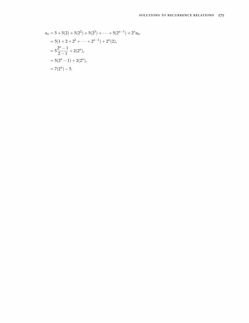
solutions to recurrence relations 275
an = 5 + 5(2) + 5(22) + 5(23) + · · ·+ 5(2n−1) + 2na0,
= 5(1 + 2 + 22 + · · ·+ 2n−1) + 2n(2),
= 52n − 12− 1
+ 2(2n),
= 5(2n − 1) + 2(2n),
= 7(2n)− 5.
276 math208: discrete mathematics
35.3 Exercises
Exercise 35.1. Guess the solution to a0 = 2, and a1 = 4, and, for n ≥ 2,
an = 4an−1 − 3an−2 and prove your guess is correct by induction.
Exercise 35.2. Solve by unfolding: a0 = 2, and, for n ≥ 1, an = 5an−1.
Exercise 35.3. Solve by unfolding: a0 = 2, and, for n ≥ 1, an = 5an−1 + 3.
36
The Method of Characteristic Roots
There is no method that will solve all recurrence relations. How-
ever, for one particular type, there is a standard technique. The type
is called a linear recurrence relation with constant coefficients. In
such a recurrence relation, the recurrence formula has the form
an = c1an−1 + c2an−2 + ... + ckan−k + f (n)
where c1, · · · , ck are constants with ck 6= 0, and f (n) is any function
of n.
The degree of the recurrence is k, the number of terms we need to
go back in the sequence to compute each new term. If f (n) = 0, then
the recurrence relation is called homogeneous. Otherwise it is called
nonhomogeneous.
In chapter 35, we noted that some simple non-homogeneous lin-
ear recurrence relations with constant coefficients can be solved by
unfolding. This method is not powerful enough for more general
problems. In this chapter we introduce a basic method that, in princi-
ple at least, can be used to solve any homogeneous linear recurrence
relation with constant coefficients.
36.1 Homogeneous, constant coefficient recursions
We begin by considering the degree 2 case. That is, we have a re-
currence relation of the form an = c1an−1 + c2an−2, for n ≥ 2,
where c1 and c2 are real constants. We must also have two initial con-
278 math208: discrete mathematics
ditions a0 and a1. That is, we are given a0 and a1 and the formula
an = c1an−1 + c2an−2, for n ≥ 2. Notice that c2 6= 0 or else we have
a linear recurrence relation with constant coefficients and degree 1.
What we seek is a closed form formula for an, which is a function of
n alone, and which is therefore independent of the previous terms of
the sequence.
36.1.1 Basic example of the method
Here’s the technique in a specific example:
The problem we will solve is to find a formula for the terms of the
sequence
a0 = 4 and a1 = 8, with
an = 4an−1 + 12an−2, for n ≥ 2.
The first thing to do is to ignore the initial conditions, and concen-
trate on the recurrence relation. And the way to solve the recurrence
relation is to guess the solution. Well, actually, it is to guess the form
of the solution1. For such a recurrence you should guess that the so- 1 An educated guess!
lution looks like an = rn, for some constant r. In other words, guess
the solution is simply the powers of some fixed number. The good
news is that this guess will always be correct! You will always find
some solutions of this form. When this guess is plugged into the
recurrence relation and the equation is simplified, the result is an
equation that can be solved for r. That equation is called the charac-
teristic equation for the recurrence. In our example, when an = rn
for each n, the result is rn = 4rn−1 + 12rn−2, and canceling rn−2 from
each term, and rearranging the equation, we get r2 − 4r − 12 = 0.
That’s the characteristic equation. The left side can be factored, and
the equation then looks like (r − 6)(r + 2) = 0, and we see the solu-
tions for r are r = 6 and r = −2. And, sure enough, if you check it
out, you will see that an = 6n and an = (−2)n both satisfy the given
the method of characteristic roots 279
recurrence relation. In other words, we find that
6n = 4 · 6n−1 + 12 · 6n−2, for all n ≥ 2, and
(−2)n = 4 · (−2)n−1 + 12 · (−2)n−2, for all n ≥ 2.
Using the characteristic equation, we have a method of finding
some solutions to a recurrence relation. This method will not find all
possible solutions however. BUT... if we find all the solutions to the
characteristic equation, then they can be combined in a certain way to
produce all possible solutions to the recurrence relation. The fact to
remember is that if r = a, b are the two solutions to the characteristic
equation (for a recurrence of order two), then every possible solution
to the linear homogenous recurrence relation must look like 2 2 Actually, that is not quite true. Thereis a slight catch to be mentioned later(see section 36.2).
αan + βbn,
for some constants α, β. In the example we have been working on,
every possible solution looks like3 3 This expression is called the generalsolution of the recurrence relation.
an = α(6)n + β(−2)n.
Once we have figured out the general solution to the recurrence
relation, it is time to think about the initial conditions. In our case,
the initial conditions are a0 = 4 and a1 = 8. The idea is to select
the constants α and β of the general solution an = α6n + β(−2)n so
it will produce the correct two initial values. For n = 0 we see we
need 4 = a0 = α60 + β(−2)0 = α + β, and for n = 1, we need
8 = a1 = α61 + β(−2)1 = 6α− 2β. Now, we solve the following pair
of equations for α and β:
α + β = 4,
6α− 2β = 8.
Performing a bit of algebra, we learn that α = 2 and β = 2. Thus the
solution to the recurrence is
an = 2 · 6n + 2 · (−2)n.
280 math208: discrete mathematics
36.1.2 Initial steps: the characteristic equation and its roots
The steps in solving a recurrence problem are:
(1) Determine the characteristic equation.
(2) Find the solutions to the characteristic equation.
(3) Write down the general solution to the recurrence relation.
(4) Select the constants in the general solution to produce the correct
initial conditions.
36.2 Repeated characteristic roots.
And now, about the little lie mentioned above: One catch with the
method of characteristic equation occurs when the equation has
repeated roots. Suppose, for example, that when the characteristic
equation is factored the result is (r − 2)(r − 2)(r − 3)(r + 5) = 0.
The characteristic roots are 2, 2, 3 and −5. Here 2 is a repeated root. If
we follow the instructions given above, then the general solution we
would write down is
an = α2n + β2n + γ3n + δ(−5)n. (36.1)
However, this expression will not include all possible solutions to the
recurrence relation. Happily, the problem is not too hard to repair:
each time a root of the characteristic equation is repeated, multiply it
by an additional factor of n in the general solution, and then proceed
with step 4 as described earlier.
For our example, we modify one of the 2n terms in equation 36.1.
The correct general solution looks like Notice the extra factor of n in the
second term.
an = α2n + βn · 2n + γ3n + δ(−5)n.
If (r− 2) had been a four fold factor of the characteristic equation4, 4 in other words, if 2 had been a charac-teristic root four times
then the part of the general solution involving the 2’s would look like
Each new occurrence of a 2 is multi-
plied by one more factor of n.α2n + βn · 2n + γn2 · 2n + δn3 · 2n.
the method of characteristic roots 281
36.3 The method of characteristic roots more formally
Let’s describe the method of characteristic equation a little more
formally. First, the characteristic equation is denoted by χ(x) = 05. Notice that the degree of χ(x) coincides with the degree of the 5 For the general degree 2 case above we
have χ(x) = x2 − c1x− c2.recurrence relation. Notice also that the non-leading coefficients of
χ(x) are simply the negatives of the coefficients of the recurrence
relation. In general, the characteristic equation of an = c1an−1 + ... +
ckan−k is
χ(x) = xk − c1xk−1 − ...− ck−1x− ck = 0.
A number r (possibly complex) is a characteristic root if χ(r) = 0.
From basic algebra we know that r is a root of a polynomial if and
only if (x− r) is a factor of the polynomial. When χ(x) is a degree 2
polynomial, by the quadratic formula, either χ(x) = (x− r1)(x− r2),
where r1 6= r2, or χ(x) = (x− r)2, for some r.
Theorem 36.1. Let c1 and c2 be real numbers. Suppose that the polynomial
χ(x) = x2 − c1x − c2 has two distinct roots r1 and r2. Then a sequence
a : N → R is a solution of the recurrence relation an = c1an−1 + c2an−2,
for n ≥ 2 if and only if am = αrm1 + βrm
2 , for all m ∈ N, and for some
constants α and β. The constants are determined by the
initial conditions (see equation 36.2).
Proof. If am = αrm1 + βrm
2 for all m ∈ N, where α and β are some
constants, then since r2i − c1ri − c2 = 0, we have r2
i = c1ri + c2, for i = 1
and n = 2. Hence, for n ≥ 2, we have
c1an−1 + c2an−2 = c1(αrn−11 + βrn−1
2 ) + c2(αrn−21 + βrn−2
2 ),
= αrn−21 (c1r1 + c2) + βrn−2
2 (c1r2 + c2), distributing and combining,
= αrn−21 · r2
1 + βrn−22 · r2
2, by the remark above,
= αrn1 + βrn
2 = an.
Conversely, if a is a solution of the recurrence relation and has initial terms
a0 and a1, then one checks that the sequence am = αrm1 + βrm
2 with
α =a1 − a0 · r2
r1 − r2, and β =
a0r1 − a1
r1 − r2(36.2)
also satisfies the relation and has the same initial conditions. The equations
282 math208: discrete mathematics
for α and β come from solving the system of linear equations
a0 = α(r1)0 + β(r2)
0 = α + β,
a1 = α(r1)1 + β(r2)
1 = αr1 + βr2.
This system is solved using techniques from a prerequisite course. ♣
Example 36.2. Solve the recurrence relation a0 = 2, a1 = 3 and an = an−2,
for n ≥ 2.
Solution. The recurrence relation is a linear homogeneous recurrence
relation of degree 2 with constant coefficients c1 = 0 and c2 = 1. The
characteristic polynomial is
χ(x) = x2 − 0 · x− 1 = x2 − 1.
The characteristic polynomial has two distinct roots since
x2 − 1 = (x− 1)(x + 1).
Let’s say r1 = 1 and r2 = −1. Then, we find the system of equations:
2 = a0 = α10 + β(−1)0 = α + β,
3 = a1 = α11 + β(−1)1 = α + β(−1) = α− β.
Adding the two equations eliminates β and gives 5 = 2α, so α = 5/2.
Substituting this into the first equation, 2 = 5/2 + β, we see that β =
−1/2. Thus, our solution is
an =52· 1n +
−12
(−1)n =52− 1
2· (−1)n.
Example 36.3. Solve the recurrence relation a1 = 3, a2 = 5, and,
an = 5an−1 − 6an−2, for n ≥ 3.
Solution. Here the characteristic polynomial is
χ(x) = x2 − 5x + 6 = (x− 2)(x− 3),
the method of characteristic roots 283
with roots r1 = 2 and r2 = 3. Now, we suppose that
am = α2m + β3m, for all m ≥ 1.
The initial conditions give rise to the system of equations
3 = a1 = α21 + β31 = 2α + 3β,
5 = a2 = α22 + β32 = 4α + 9β.
If we multiply the top equation through by 2, we obtain
6 = 4α + 6β,
5 = 4α + 9β.
Subtracting the second equation from the first eliminates α and yields
1 = −3β. So, we have found that β = −1/3. Substitution into the
first equation yields 3 = 2α + 3 · (−1/3), so α = 2. Thus
am = 2 · 2m − 13· 3m = 2m+1 − 3m−1, for all m ≥ 1.
36.4 The method for repeated roots
The other case we mentioned had a characteristic polynomial of
degree two with one repeated root. Since the proof is similar we
simply state the theorem.
Theorem 36.4. Let c1 and c2 be real numbers with c2 6= 0 and suppose
that the polynomial x2 − c1x − c2 has a root r with multiplicity 2, so that
x2 − c1x− c2 = (x− r)2. Then, a sequence a : N → R is a solution of the
recurrence relation an = c1an−1 + c2an−2, for n ≥ 2 if and only if
am = (α + βm)rm,
for all m ∈N, and for some constants α and β.
Example 36.5. Solve the recurrence relation a0 = −1, a1 = 4 and an =
4an−1 − 4an−2, for n ≥ 2.
Solution. In this case we have χ(x) = x2 − 4x + 4 = (x − 2)2. So, we
284 math208: discrete mathematics
may suppose that
am = (α + βm)2m, for all m ∈N.
The initial conditions give rise to the system of equations
−1 = a0 = (α + β · 0)20 = (α) · 1 = α,
4 = a1 = (α + β · 1)21 = 2(α + β) · 2.
Substituting α = −1 into the second equation gives 4 = 2(β − 1), so
2 = β− 1 and β = 3. Therefore am = (3m− 1)2m, for all m ∈N.
36.5 The general case
Finally, we state6 the general method of characteristic roots. 6 without proof
Theorem 36.6. Let c1, c2, ..., ck ∈ R with ck 6= 0. Suppose that the
characteristic polynomial factors as
χ(x) = xk − c1xk−1 − c2xk−2 − ...− ck−1x− ck,
= (x− r1)j1(x− r2)
j2 · · · (x− rs)js ,
where r1, r2, . . ., rs are distinct roots of χ(x), and j1, j2, . . ., js are positive
integers such that
j1 + j2 + j3 + ... + js = k.
Then a sequence a : N→ R is a solution of the recurrence relation
an = c1an−1 + c2an−2 + ... + ckan−k, for n ≥ k
if and only if
am = p1(m)rm1 + p2(m)rm
2 + ... + ps(m)rms , for all m ∈N,
where
pi(m) = α0,i + α1,im + α2,im2 + ... + αji−1,imji−1, 1 ≤ i ≤ s
and the αl,i’s are constants.
the method of characteristic roots 285
There is a problem with the general case. It is true that given the
recurrence relation we can simply write down the characteristic poly-
nomial. However it can be quite a challenge to factor it as required
by the theorem. Even if we succeed in factoring it we are faced with
the tedious task of setting up and solving a system of k linear equa-
tions in k unknowns (the αl,i’s). While in theory such a system can be
solved using the methods of elimination or substitution covered in a
college algebra course, in practice, the amount of labor involved can
become overwhelming. For this reason, computer algebra systems are
often used in practice to help solve systems of equations, or even the
original recurrence relation.
286 math208: discrete mathematics
36.6 Exercises
Exercise 36.1. For each of the following sequences find a recurrence relation
satisfied by the sequence. Include a sufficient number of initial conditions to
completely specify the sequence.
(a) an = 2n + 3, n ≥ 0
(b) an = 3 · 2n, n ≥ 1
(c) an = n2, n ≥ 1
(d) an = n + (−1)n, n ≥ 0
Solve each of the following recurrence relations:
Exercise 36.2. a0 = 3, a1 = 6, and an = an−1 + 6an−2, for n ≥ 2.
Exercise 36.3. a0 = 4, a1 = 7, and an = 5an−1 − 6an−2, for n ≥ 2.
Exercise 36.4. a2 = 5, a3 = 13, and an = 7an−1 − 10an−2, for n ≥ 4.
Exercise 36.5. a1 = 3, a2 = 5, and an = 4an−1 − 4an−2, for n ≥ 3.
Exercise 36.6. a0 = 1, a1 = 6, and an = 6an−1 − 9an−2, for n ≥ 2.
Exercise 36.7. a1 = 2, a2 = 8, and an = an−2, for n ≥ 3.
Exercise 36.8. a0 = 2, a1 = 5, a2 = 15, and an = 6an−1 − 11an−2 +
6an−3, for n ≥ 3.
Exercise 36.9. Find a closed form formula for the terms of the Fibonacci
sequence: f0 = 0, f1 = 1, and for n ≥ 2, fn = fn−1 + fn−2.
37
Solving Nonhomogeneous Recurrences
When a linear recurrence relation with constant coefficients
for a sequence {sn} looks like
sn = c1sn−1 + c2sn−2 + · · ·+ cksn−k + f (n),
where f (n) is some (nonzero) function of n, then the recurrence rela-
tion is said to be nonhomogeneous. For example, sn = 2sn−1 + n2 + 1
is a nonhomogeneous recurrence. Here f (n) = n2 + 1. The methods
used in the last chapter are not adequate to deal with nonhomoge-
neous problems. But it wasn’t all a waste since those methods do
provide one step in the solution of nonhomogeneous problems.
37.1 Steps to solve nonhomogeneous recurrence relations
Step (1): Replace the f (n) by 0 to create a homogeneous recurrence relation,
sn = c1sn−1 + c2sn−2 + · · ·+ cksn−k.
Now solve this and write down the general solution1. For exam- 1 We learned to do this in chapter 36.
ple, in the case of no repeated roots, the general solution will look
something like:
sn = a1rn1 + a2rn
2 + · · ·+ akrnk ,
where the constants a1, a2, · · · , ak are to be determined.
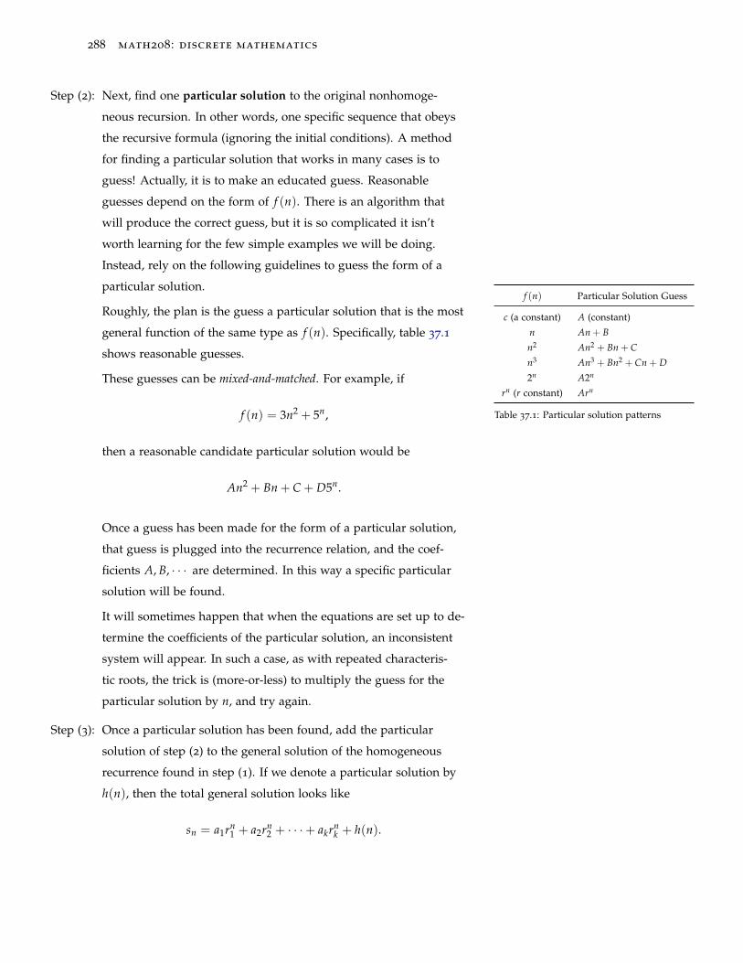
288 math208: discrete mathematics
Step (2): Next, find one particular solution to the original nonhomoge-
neous recursion. In other words, one specific sequence that obeys
the recursive formula (ignoring the initial conditions). A method
for finding a particular solution that works in many cases is to
guess! Actually, it is to make an educated guess. Reasonable
guesses depend on the form of f (n). There is an algorithm that
will produce the correct guess, but it is so complicated it isn’t
worth learning for the few simple examples we will be doing.
Instead, rely on the following guidelines to guess the form of a
particular solution.
Roughly, the plan is the guess a particular solution that is the most
general function of the same type as f (n). Specifically, table 37.1
shows reasonable guesses.
f (n) Particular Solution Guess
c (a constant) A (constant)
n An + B
n2 An2 + Bn + C
n3 An3 + Bn2 + Cn + D
2n A2n
rn (r constant) Arn
Table 37.1: Particular solution patterns
These guesses can be mixed-and-matched. For example, if
f (n) = 3n2 + 5n,
then a reasonable candidate particular solution would be
An2 + Bn + C + D5n.
Once a guess has been made for the form of a particular solution,
that guess is plugged into the recurrence relation, and the coef-
ficients A, B, · · · are determined. In this way a specific particular
solution will be found.
It will sometimes happen that when the equations are set up to de-
termine the coefficients of the particular solution, an inconsistent
system will appear. In such a case, as with repeated characteris-
tic roots, the trick is (more-or-less) to multiply the guess for the
particular solution by n, and try again.
Step (3): Once a particular solution has been found, add the particular
solution of step (2) to the general solution of the homogeneous
recurrence found in step (1). If we denote a particular solution by
h(n), then the total general solution looks like
sn = a1rn1 + a2rn
2 + · · ·+ akrnk + h(n).
solving nonhomogeneous recurrences 289
Step (4): Invoke the initial conditions to determine the values of the coeffi-
cients a1, a2, · · · , ak just as we did for the homogeneous problems
in chapter 36.
The major oversight made solving a nonhomogeneous recurrence
relation is trying to determine the coefficients a1, a2, · · · , ak before the
particular solution is added to the general solution. This mistake will
usually lead to inconsistent information about the coefficients, and no
solution to the recurrence will be found.
37.2 Examples
Example 37.1. Let’s solve the Tower of Hanoi recurrence using this method.
The recurrence is H0 = 0, and, for n ≥ 1, Hn = 2Hn−1 + 1. We know
the closed form formula for Hn is 2n − 1 already, but let’s work it out using
the method outlined above.
Step (1): Find the general solution of related homogeneous recursion (indicated by
the superscript (h)): H(h)n = 2H(h)
n−1. That will be H(h)n = A2n.
Step (2): Guess the particular solution (indicated by superscript (p)): H(p)n = B, a
constant. Plugging that guess into the recurrence gives B = 2B + 1, and
so we see B = −1.
Step (3): Hence, the general solution to the Tower of Hanoi recurrence is
Hn = H(h)n + H(p)
n = A2n − 1.
Step (4): Now, use the initial condition to determine A: When n = 0, we want
0 = A20 − 1 which means A = 1. Thus, we find the expected result:
Hn = 2n − 1, for n ≥ 0.
290 math208: discrete mathematics
Example 37.2. Here is a more complicated example worked out in detail to
exhibit the method. Let’s solve the recurrence
s1 = 2, s2 = 5 and,
sn = sn−1 + 6sn−2 + 3n− 1, for n ≥ 3.
Step (1): Find the general solution of sn = sn−1 + 6sn−2. After finding the
characteristic equation, and the characteristic roots, the general solution
turns out to be sn = a13n + a2(−2)n.
Step (2): To find a particular solution let’s guess that there is a solution h(n) that
looks like h(n) = an + b, where a and b are to be determined. To find
values of a and b that work, we substitute this guess for a solution into
the original recurrence relation. In this case, the result of plugging in the
guess (sn = h(n) = an + b) gives us:
an + b = a(n− 1) + b + 6(a(n− 2) + b) + 3n− 1.
which can be rearranged to
(6a + 3)n + (−13a + 6b− 1) = 0.
If this equation is to be correct for all n, then, in particular, it must be
correct when n = 0 and when n = 1, and that tells us that
−13a + 6b− 1 = 0 and,
6a + 3− 13a + 6b− 1 = 0.
Solving this pair of equations we find a = − 12 and b = − 11
12 . And, sure
enough, if you plug this alleged solution into the original recurrence, you
will see it checks.
Step (3): Write down the general solution to the original nonhomogeneous problem
by adding the particular solution of step (2) to the general solution from
step (1) getting:
sn = a13n + a2(−2)n +
(−1
2
)n +
(−11
12
).
solving nonhomogeneous recurrences 291
Step (4): Now a1, a2 can be calculated: For n = 1, the first initial condition gives
2 = a131 + a2(−2)1 +
(−1
2
)1 +
(−11
12
),
and for n = 2, we get
5 = a132 + a2(−2)2 +
(−1
2
)2 +
(−11
12
).
Solving these two equations for a1 and a2, we find that a1 = 1112 and
a2 = − 13 .
So the solution to the recurrence is
sn =1112
3n − 13(−2)n +
(−1
2
)n +
(−11
12
).
292 math208: discrete mathematics
37.3 Exercises
Use the general solutions for the related homogeneous problems of chapter 36
to help solve the following nonhomogeneous recurrence relations with initial
conditions.
Exercise 37.1. a0 = 3, a1 = 6 and an = an−1 + 6an−2 + 1, for n ≥ 2.
Exercise 37.2. a2 = 5, a3 = 13 and an = 7an−1 − 10an−2 + n, for n ≥ 4.
Exercise 37.3. a0 = 0, a1 = 1 and an = 4an−1 − 4an−2 + 2n, for n ≥ 2.
Exercise 37.4. a0 = 1, a1 = 6 and an = 6an−1 − 9an−2 + n, for n ≥ 2.
Exercise 37.5. a0 = 2, a1 = 5, a2 = 15, and an = 6an−1 − 11an−2 +
6an−3 + 2n + 1, for n ≥ 3.
38
Graphs
In an earlier chapter we represented relations with a
graph. In this chapter we discuss a more general notion
of a graph.
38.1 Some Graph Terminology
There is a lot of new vocabulary to absorb concerning graphs! For
this chapter, a graph will consist of a number of points (called ver-
tices) (singular: vertex) together with lines (called edges) joining
some (possibly none, possibly all) pairs of vertices. Unlike the graphs
of earlier chapters, we will not allow an edge from a vertex back to
itself (so no loops allowed), we will not allow multiple edges between
vertices, and the edges will not be directed (there will be no edges
with arrowheads on one or both ends). All of our graphs will have a
finite vertex sets, and consequently a finite number of edges. Graphs
are typically denoted by an uppercase letter such as G or H.
If you would like a formal definition: a graph, G consists of a set
of vertices V and a set E of edges, where an edge t ∈ E is written as
an unordered pair of vertices {u, v}, (in other words, a set consisting
of two different vertices). We say that the edge t = {u, v} has end-
points u and v, and that the edge t is incident to both u and v. The
vertices u and v are adjacent when there is an edge with endpoints
u and v; otherwise they are not adjacent. Such a formal definition is
necessary, but a more helpful way to think of a graph is as a diagram.
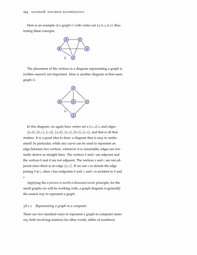
294 math208: discrete mathematics
Here is an example of a graph G with vertex set {a, b, c, d, e} illus-
trating these concepts.
a
b c
d
eG
The placement of the vertices in a diagram representing a graph is
(within reason!) not important. Here is another diagram of that same
graph G.
a b c
d
e
G
In this diagram, we again have vertex set a, b, c, d, e, and edges
{a, b}, {b, c}, {c, d}, {a, d}, {a, e}, {b, e}, {c, e}, and that is all that
matters. It is a good idea to draw a diagram that is easy to under-
stand! In particular, while any curve can be used to represent an
edge between two vertices, whenever it is reasonable, edges are nor-
mally drawn as straight lines. The vertices b and e are adjacent and
the vertices b and d are not adjacent. The vertices a and c are not ad-
jacent since there is no edge {a, c}. If we use s to denote the edge
joining b to c, then s has endpoints b and c, and s is incident to b and
c.
Applying the a-picture-is-worth-a-thousand-words principle, for the
small graphs we will be working with, a graph diagram is generally
the easiest way to represent a graph.
38.1.1 Representing a graph in a computer
There are two standard ways to represent a graph in computer mem-
ory, both involving matrices (in other words, tables of numbers).
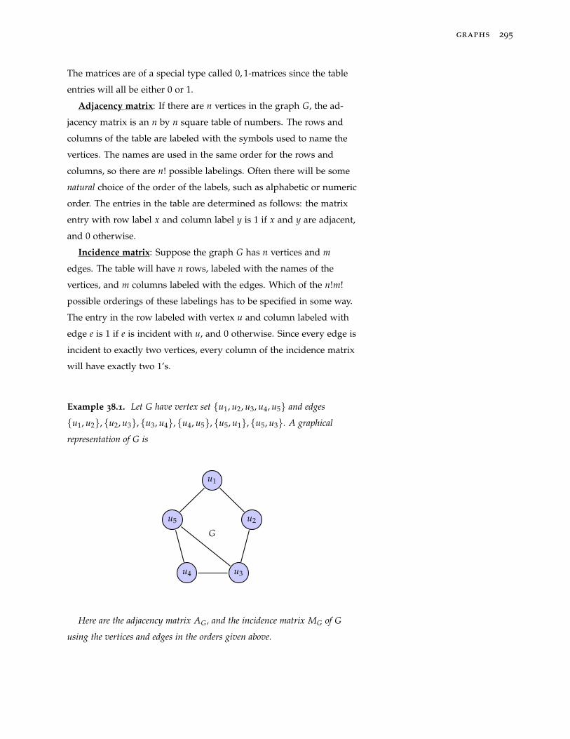
graphs 295
The matrices are of a special type called 0, 1-matrices since the table
entries will all be either 0 or 1.
Adjacency matrix: If there are n vertices in the graph G, the ad-
jacency matrix is an n by n square table of numbers. The rows and
columns of the table are labeled with the symbols used to name the
vertices. The names are used in the same order for the rows and
columns, so there are n! possible labelings. Often there will be some
natural choice of the order of the labels, such as alphabetic or numeric
order. The entries in the table are determined as follows: the matrix
entry with row label x and column label y is 1 if x and y are adjacent,
and 0 otherwise.
Incidence matrix: Suppose the graph G has n vertices and m
edges. The table will have n rows, labeled with the names of the
vertices, and m columns labeled with the edges. Which of the n!m!
possible orderings of these labelings has to be specified in some way.
The entry in the row labeled with vertex u and column labeled with
edge e is 1 if e is incident with u, and 0 otherwise. Since every edge is
incident to exactly two vertices, every column of the incidence matrix
will have exactly two 1’s.
Example 38.1. Let G have vertex set {u1, u2, u3, u4, u5} and edges
{u1, u2}, {u2, u3}, {u3, u4}, {u4, u5}, {u5, u1}, {u5, u3}. A graphical
representation of G is
u5
u1
u2
u3u4
G
Here are the adjacency matrix AG, and the incidence matrix MG of G
using the vertices and edges in the orders given above.
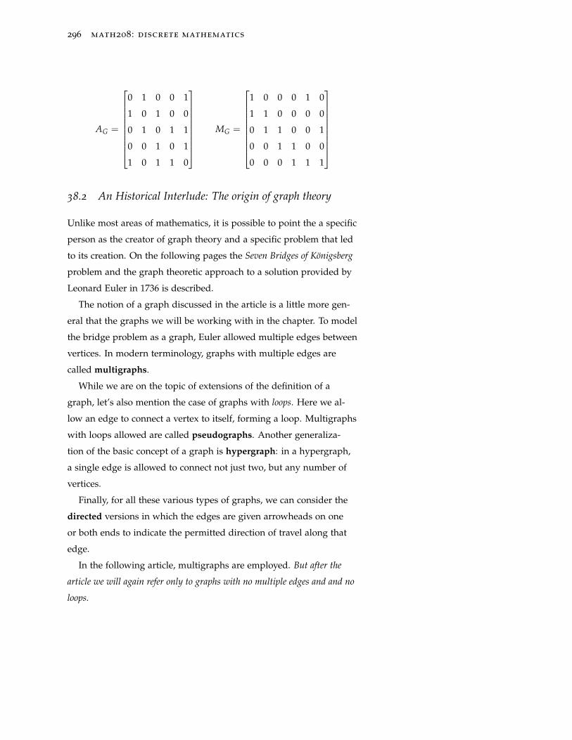
296 math208: discrete mathematics
AG =
0 1 0 0 1
1 0 1 0 0
0 1 0 1 1
0 0 1 0 1
1 0 1 1 0
MG =
1 0 0 0 1 0
1 1 0 0 0 0
0 1 1 0 0 1
0 0 1 1 0 0
0 0 0 1 1 1
38.2 An Historical Interlude: The origin of graph theory
Unlike most areas of mathematics, it is possible to point the a specific
person as the creator of graph theory and a specific problem that led
to its creation. On the following pages the Seven Bridges of Königsberg
problem and the graph theoretic approach to a solution provided by
Leonard Euler in 1736 is described.
The notion of a graph discussed in the article is a little more gen-
eral that the graphs we will be working with in the chapter. To model
the bridge problem as a graph, Euler allowed multiple edges between
vertices. In modern terminology, graphs with multiple edges are
called multigraphs.
While we are on the topic of extensions of the definition of a
graph, let’s also mention the case of graphs with loops. Here we al-
low an edge to connect a vertex to itself, forming a loop. Multigraphs
with loops allowed are called pseudographs. Another generaliza-
tion of the basic concept of a graph is hypergraph: in a hypergraph,
a single edge is allowed to connect not just two, but any number of
vertices.
Finally, for all these various types of graphs, we can consider the
directed versions in which the edges are given arrowheads on one
or both ends to indicate the permitted direction of travel along that
edge.
In the following article, multigraphs are employed. But after the
article we will again refer only to graphs with no multiple edges and and no
loops.
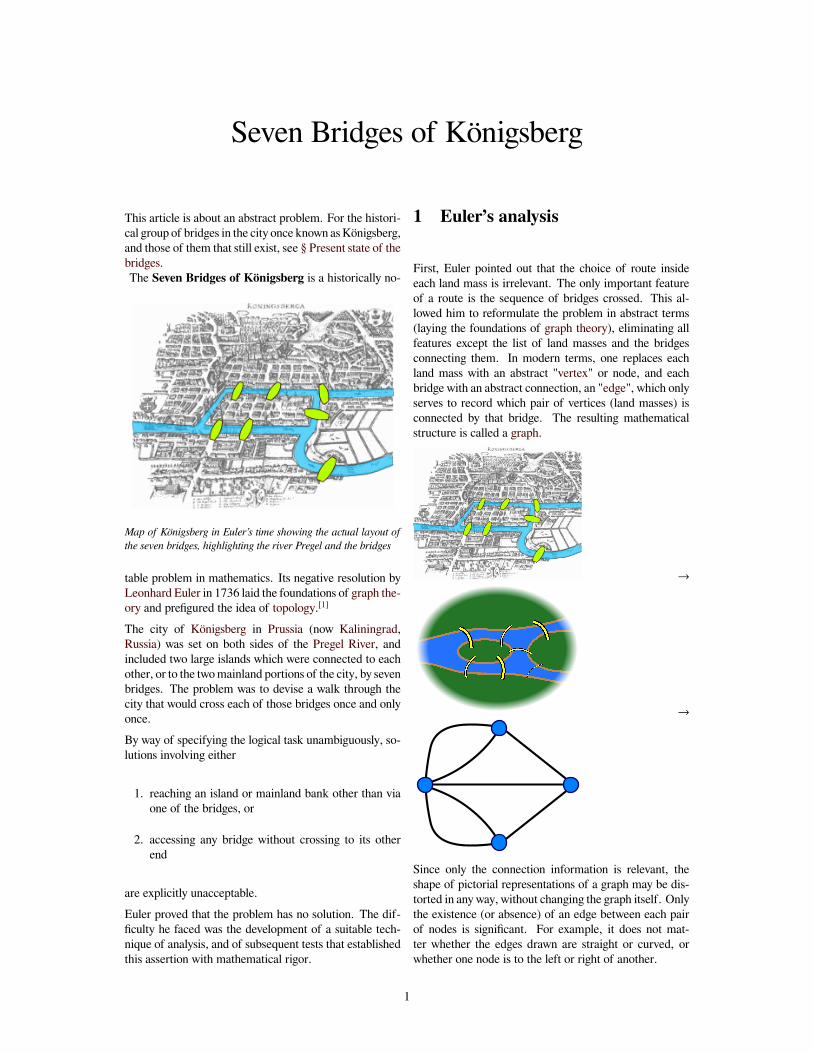
Seven Bridges of Königsberg
This article is about an abstract problem. For the histori-cal group of bridges in the city once known as Königsberg,and those of them that still exist, see § Present state of thebridges.The Seven Bridges of Königsberg is a historically no-
Map of Königsberg in Euler’s time showing the actual layout ofthe seven bridges, highlighting the river Pregel and the bridges
table problem in mathematics. Its negative resolution byLeonhard Euler in 1736 laid the foundations of graph the-ory and prefigured the idea of topology.[1]
The city of Königsberg in Prussia (now Kaliningrad,Russia) was set on both sides of the Pregel River, andincluded two large islands which were connected to eachother, or to the twomainland portions of the city, by sevenbridges. The problem was to devise a walk through thecity that would cross each of those bridges once and onlyonce.By way of specifying the logical task unambiguously, so-lutions involving either
1. reaching an island or mainland bank other than viaone of the bridges, or
2. accessing any bridge without crossing to its otherend
are explicitly unacceptable.Euler proved that the problem has no solution. The dif-ficulty he faced was the development of a suitable tech-nique of analysis, and of subsequent tests that establishedthis assertion with mathematical rigor.
1 Euler’s analysis
First, Euler pointed out that the choice of route insideeach land mass is irrelevant. The only important featureof a route is the sequence of bridges crossed. This al-lowed him to reformulate the problem in abstract terms(laying the foundations of graph theory), eliminating allfeatures except the list of land masses and the bridgesconnecting them. In modern terms, one replaces eachland mass with an abstract "vertex" or node, and eachbridge with an abstract connection, an "edge", which onlyserves to record which pair of vertices (land masses) isconnected by that bridge. The resulting mathematicalstructure is called a graph.
→
→
Since only the connection information is relevant, theshape of pictorial representations of a graph may be dis-torted in any way, without changing the graph itself. Onlythe existence (or absence) of an edge between each pairof nodes is significant. For example, it does not mat-ter whether the edges drawn are straight or curved, orwhether one node is to the left or right of another.
1
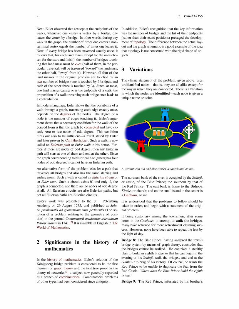
2 3 VARIATIONS
Next, Euler observed that (except at the endpoints of thewalk), whenever one enters a vertex by a bridge, oneleaves the vertex by a bridge. In other words, during anywalk in the graph, the number of times one enters a non-terminal vertex equals the number of times one leaves it.Now, if every bridge has been traversed exactly once, itfollows that, for each land mass (except for the ones cho-sen for the start and finish), the number of bridges touch-ing that land mass must be even (half of them, in the par-ticular traversal, will be traversed “toward” the landmass;the other half, “away” from it). However, all four of theland masses in the original problem are touched by anodd number of bridges (one is touched by 5 bridges, andeach of the other three is touched by 3). Since, at most,two land masses can serve as the endpoints of a walk, theproposition of a walk traversing each bridge once leads toa contradiction.In modern language, Euler shows that the possibility of awalk through a graph, traversing each edge exactly once,depends on the degrees of the nodes. The degree of anode is the number of edges touching it. Euler’s argu-ment shows that a necessary condition for the walk of thedesired form is that the graph be connected and have ex-actly zero or two nodes of odd degree. This conditionturns out also to be sufficient—a result stated by Eulerand later proven by Carl Hierholzer. Such a walk is nowcalled an Eulerian path or Euler walk in his honor. Fur-ther, if there are nodes of odd degree, then any Eulerianpath will start at one of them and end at the other. Sincethe graph corresponding to historical Königsberg has fournodes of odd degree, it cannot have an Eulerian path.An alternative form of the problem asks for a path thattraverses all bridges and also has the same starting andending point. Such a walk is called an Eulerian circuit oran Euler tour. Such a circuit exists if, and only if, thegraph is connected, and there are no nodes of odd degreeat all. All Eulerian circuits are also Eulerian paths, butnot all Eulerian paths are Eulerian circuits.Euler’s work was presented to the St. PetersburgAcademy on 26 August 1735, and published as Solu-tio problematis ad geometriam situs pertinentis (The so-lution of a problem relating to the geometry of posi-tion) in the journal Commentarii academiae scientiarumPetropolitanae in 1741.[2] It is available in English in TheWorld of Mathematics.
2 Significance in the history ofmathematics
In the history of mathematics, Euler’s solution of theKönigsberg bridge problem is considered to be the firsttheorem of graph theory and the first true proof in thetheory of networks,[3] a subject now generally regardedas a branch of combinatorics. Combinatorial problemsof other types had been considered since antiquity.
In addition, Euler’s recognition that the key informationwas the number of bridges and the list of their endpoints(rather than their exact positions) presaged the develop-ment of topology. The difference between the actual lay-out and the graph schematic is a good example of the ideathat topology is not concerned with the rigid shape of ob-jects.
3 Variations
The classic statement of the problem, given above, usesunidentified nodes—that is, they are all alike except forthe way in which they are connected. There is a variationin which the nodes are identified—each node is given aunique name or color.
A variant with red and blue castles, a church and an inn.
The northern bank of the river is occupied by the Schloß,or castle, of the Blue Prince; the southern by that ofthe Red Prince. The east bank is home to the Bishop’sKirche, or church; and on the small island in the center isa Gasthaus, or inn.It is understood that the problems to follow should betaken in order, and begin with a statement of the origi-nal problem:It being customary among the townsmen, after somehours in the Gasthaus, to attempt to walk the bridges,many have returned for more refreshment claiming suc-cess. However, none have been able to repeat the feat bythe light of day.Bridge 8: The Blue Prince, having analyzed the town’sbridge system by means of graph theory, concludes thatthe bridges cannot be walked. He contrives a stealthyplan to build an eighth bridge so that he can begin in theevening at his Schloß, walk the bridges, and end at theGasthaus to brag of his victory. Of course, he wants theRed Prince to be unable to duplicate the feat from theRed Castle. Where does the Blue Prince build the eighthbridge?
Bridge 9: The Red Prince, infuriated by his brother’s
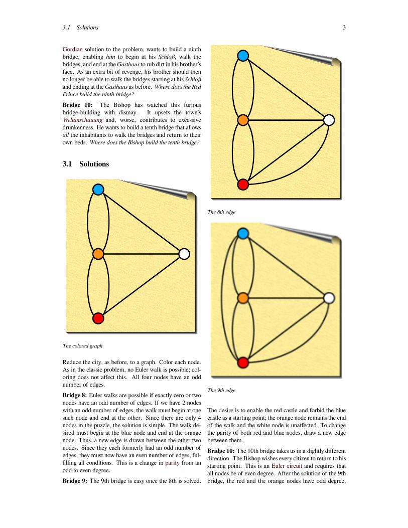
3.1 Solutions 3
Gordian solution to the problem, wants to build a ninthbridge, enabling him to begin at his Schloß, walk thebridges, and end at theGasthaus to rub dirt in his brother’sface. As an extra bit of revenge, his brother should thenno longer be able to walk the bridges starting at his Schloßand ending at theGasthaus as before. Where does the RedPrince build the ninth bridge?
Bridge 10: The Bishop has watched this furiousbridge-building with dismay. It upsets the town’sWeltanschauung and, worse, contributes to excessivedrunkenness. He wants to build a tenth bridge that allowsall the inhabitants to walk the bridges and return to theirown beds. Where does the Bishop build the tenth bridge?
3.1 Solutions
The colored graph
Reduce the city, as before, to a graph. Color each node.As in the classic problem, no Euler walk is possible; col-oring does not affect this. All four nodes have an oddnumber of edges.Bridge 8: Euler walks are possible if exactly zero or twonodes have an odd number of edges. If we have 2 nodeswith an odd number of edges, the walk must begin at onesuch node and end at the other. Since there are only 4nodes in the puzzle, the solution is simple. The walk de-sired must begin at the blue node and end at the orangenode. Thus, a new edge is drawn between the other twonodes. Since they each formerly had an odd number ofedges, they must now have an even number of edges, ful-filling all conditions. This is a change in parity from anodd to even degree.Bridge 9: The 9th bridge is easy once the 8th is solved.
The 8th edge
The 9th edge
The desire is to enable the red castle and forbid the bluecastle as a starting point; the orange node remains the endof the walk and the white node is unaffected. To changethe parity of both red and blue nodes, draw a new edgebetween them.Bridge 10: The 10th bridge takes us in a slightly differentdirection. The Bishop wishes every citizen to return to hisstarting point. This is an Euler circuit and requires thatall nodes be of even degree. After the solution of the 9thbridge, the red and the orange nodes have odd degree,
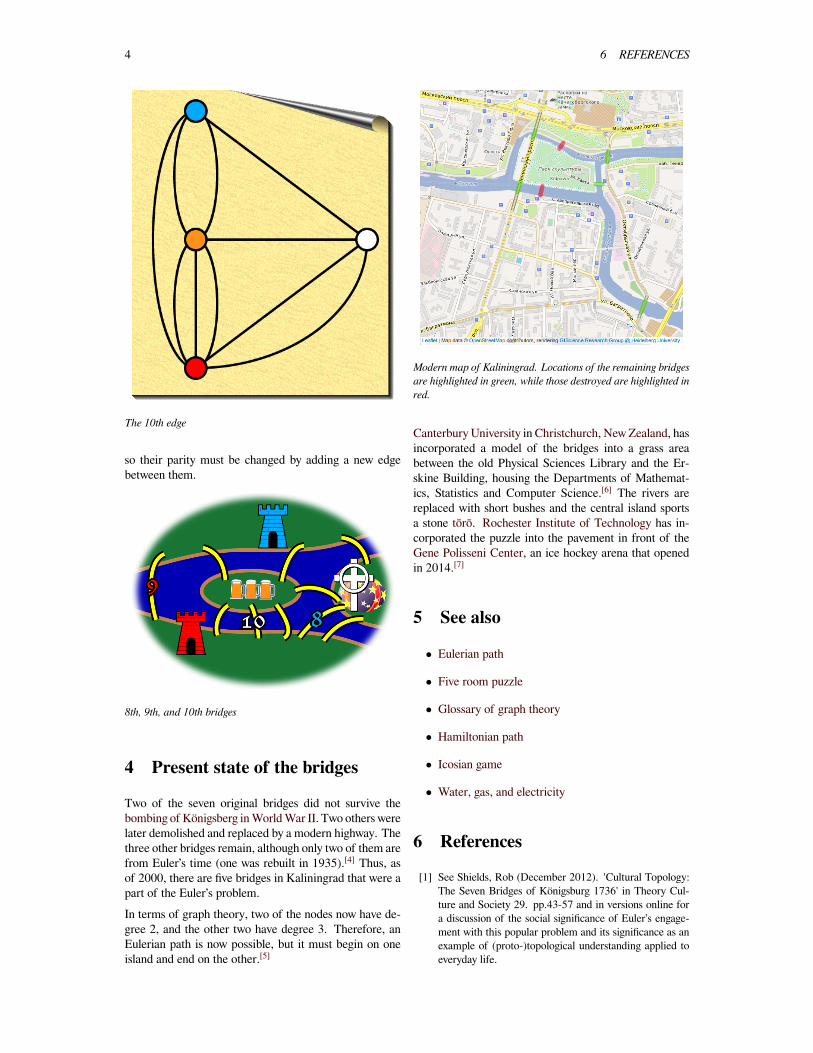
4 6 REFERENCES
The 10th edge
so their parity must be changed by adding a new edgebetween them.
8th, 9th, and 10th bridges
4 Present state of the bridges
Two of the seven original bridges did not survive thebombing of Königsberg inWorldWar II. Two others werelater demolished and replaced by a modern highway. Thethree other bridges remain, although only two of them arefrom Euler’s time (one was rebuilt in 1935).[4] Thus, asof 2000, there are five bridges in Kaliningrad that were apart of the Euler’s problem.In terms of graph theory, two of the nodes now have de-gree 2, and the other two have degree 3. Therefore, anEulerian path is now possible, but it must begin on oneisland and end on the other.[5]
Modern map of Kaliningrad. Locations of the remaining bridgesare highlighted in green, while those destroyed are highlighted inred.
Canterbury University in Christchurch, NewZealand, hasincorporated a model of the bridges into a grass areabetween the old Physical Sciences Library and the Er-skine Building, housing the Departments of Mathemat-ics, Statistics and Computer Science.[6] The rivers arereplaced with short bushes and the central island sportsa stone tōrō. Rochester Institute of Technology has in-corporated the puzzle into the pavement in front of theGene Polisseni Center, an ice hockey arena that openedin 2014.[7]
5 See also
• Eulerian path
• Five room puzzle
• Glossary of graph theory
• Hamiltonian path
• Icosian game
• Water, gas, and electricity
6 References
[1] See Shields, Rob (December 2012). 'Cultural Topology:The Seven Bridges of Königsburg 1736' in Theory Cul-ture and Society 29. pp.43-57 and in versions online fora discussion of the social significance of Euler’s engage-ment with this popular problem and its significance as anexample of (proto-)topological understanding applied toeveryday life.
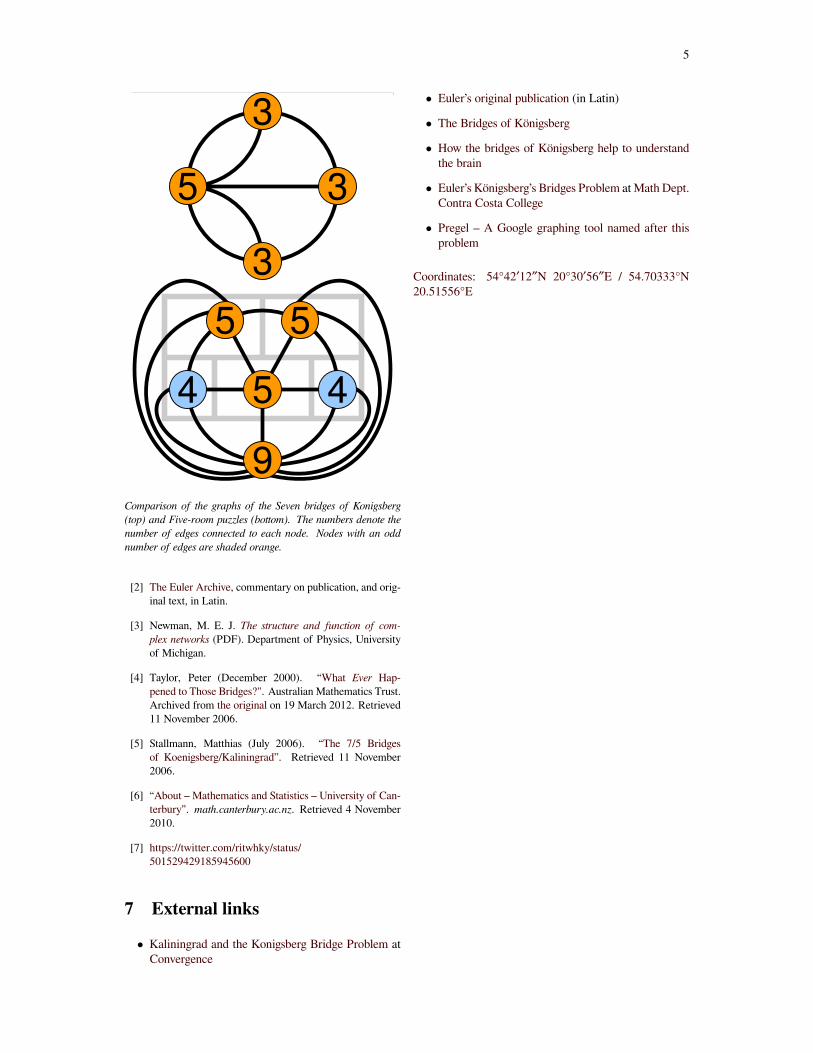
5
5 3
3
3
5 5
54 4
9Comparison of the graphs of the Seven bridges of Konigsberg(top) and Five-room puzzles (bottom). The numbers denote thenumber of edges connected to each node. Nodes with an oddnumber of edges are shaded orange.
[2] The Euler Archive, commentary on publication, and orig-inal text, in Latin.
[3] Newman, M. E. J. The structure and function of com-plex networks (PDF). Department of Physics, Universityof Michigan.
[4] Taylor, Peter (December 2000). “What Ever Hap-pened to Those Bridges?". Australian Mathematics Trust.Archived from the original on 19 March 2012. Retrieved11 November 2006.
[5] Stallmann, Matthias (July 2006). “The 7/5 Bridgesof Koenigsberg/Kaliningrad”. Retrieved 11 November2006.
[6] “About – Mathematics and Statistics – University of Can-terbury”. math.canterbury.ac.nz. Retrieved 4 November2010.
[7] https://twitter.com/ritwhky/status/501529429185945600
7 External links
• Kaliningrad and the Konigsberg Bridge Problem atConvergence
• Euler’s original publication (in Latin)
• The Bridges of Königsberg
• How the bridges of Königsberg help to understandthe brain
• Euler’s Königsberg’s Bridges Problem at Math Dept.Contra Costa College
• Pregel – A Google graphing tool named after thisproblem
Coordinates: 54°42′12″N 20°30′56″E / 54.70333°N20.51556°E
6 8 TEXT AND IMAGE SOURCES, CONTRIBUTORS, AND LICENSES
8 Text and image sources, contributors, and licenses
8.1 Text• Seven Bridges of Königsberg Source: https://en.wikipedia.org/wiki/Seven_Bridges_of_K%C3%B6nigsberg?oldid=759230125 Contrib-
utors: Zundark, Eclecticology, Deb, D, Michael Hardy, Chris-martin, Gabbe, Seav, Den fjättrade ankan~enwiki, Mark Foskey, Bogdan-giusca, Berteun, Ed Cormany, Reddi, Dysprosia, Wik, Shizhao, AnonMoos, Jerzy, Robbot, Murray Langton, Fredrik, Donreed, Altenmann,Kneiphof, Bkell, Matt Gies, Giftlite, JamesMLane, Harp, MSGJ, Dratman, Finn-Zoltan, Macrakis, Matthead, Gadfium, Antandrus, DRE,Icairns, Ukexpat, Clubjuggle, Deadlock, Wikiacc, Ascánder, Bender235, Shanes, C S, Blotwell, La goutte de pluie, AllTom, Arthena,Keenan Pepper, Cdc, Americanadian, Oghmoir, Gene Nygaard, Alai, Ghirlandajo, Hq3473, Jftsang, Apokrif, Tabletop, Cbdorsett, Au-diovideo, Xiong, Marudubshinki, StefanFuhrmann~enwiki, Graham87, BD2412, Qwertyus, Salix alba, Mkehrt, FlaBot, Gurch, Bgwhite,YurikBot, Wavelength, Hairy Dude, Snillet, Michael Slone, Sikon, Stallions2010, CptnMisc, Arthur Rubin, Cmglee, DVD R W, Smack-Bot, McGeddon, Stegano~enwiki, Wzhao553, Betacommand, Anachronist, Bird of paradox, Thumperward, DHN-bot~enwiki, Scray, JohnReid, LtPowers, John, JLeander, NongBot~enwiki, DaBjork, TheFarix, BranStark, Dilip rajeev, Eyefragment, Courcelles, Stuart Wim-bush, CmdrObot, Ivan Pozdeev, Phauly, Nalpdii~enwiki, Nczempin, WLior, Iempleh, Thijs!bot, Headbomb, Lethargy, Gswitz, Seaphoto,Smith2006, Hurmari, JAnDbot, MER-C, CheMechanical, The Anomebot2, David Eppstein, WPaulB, DerHexer, Gwern, LapisQuem,R'n'B, CommonsDelinker, Nev1, Maproom, Smitty, Independentdependent, TXiKiBoT, David Condrey, LFStokols, Falcon8765, Dusti,YonaBot, Hertz1888, Triwbe, Smsarmad, Foljiny, Ctxppc, Ken123BOT, Nic bor, Mikeharris111, Pnijssen, ClueBot, Kl4m, CounterVan-dalismBot, Piledhigheranddeeper, Excirial, Steveheric, Manu-ve Pro Ski, Jth1994, Addbot, Andunie, Godwin100, Fottry55i6, LinkFA-Bot, Numbo3-bot, Komischn, PV=nRT, Teles, Zorrobot, Luckas-bot, Yobot, AnakngAraw, Ciphers, Materialscientist, Smmlit, ArthurBot,Obersachsebot, Xqbot, Zevyefa, RibotBOT, Tmgreen, Zmorell, Chenopodiaceous, AstaBOTh15, Winterst, MarcelB612, Bmclaughlin9,Serols, Christopher1968, MFrawn, Nascar1996, Deadlyops, WikitanvirBot, TuHan-Bot, Thecheesykid, Cobaltcigs, Donaldm314, Don-ner60, Scientific29, Orange Suede Sofa, Haythamdouaihy, ClueBot NG, Lord Chamberlain, the Renowned, Vacation9, Santacloud, Ianr790,Athos, MusikAnimal, Cyberbot II, Dexbot, Hmainsbot1, Christallkeks, RockvilleRideOn, Ynaamad, MasterTriangle12, Monkbot, Acekqj,Blois2014, Imdifferentyo123456789, Poppy sheppard and Anonymous: 170
8.2 Images• File:7_bridges.svg Source: https://upload.wikimedia.org/wikipedia/commons/9/91/7_bridges.svg License: CC-BY-SA-3.0 Contributors:
? Original artist: ?• File:7_bridgesID.png Source: https://upload.wikimedia.org/wikipedia/commons/b/b3/7_bridgesID.png License: CC-BY-SA-3.0 Con-
tributors: Transferred from en.wikipedia to Commons. Original artist: The original uploader was Xiong at English Wikipedia• File:7b-graph09.png Source: https://upload.wikimedia.org/wikipedia/commons/6/69/7b-graph09.png License: CC-BY-SA-3.0 Contrib-
utors: Transferred from en.wikipedia to Commons. Original artist: Xiong at English Wikipedia• File:Commons-logo.svg Source: https://upload.wikimedia.org/wikipedia/en/4/4a/Commons-logo.svg License: PD Contributors: ? Origi-
nal artist: ?• File:Comparison_7_bridges_of_Konigsberg_5_room_puzzle_graphs.svg Source: https://upload.wikimedia.org/wikipedia/
commons/f/fb/Comparison_7_bridges_of_Konigsberg_5_room_puzzle_graphs.svg License: CC BY-SA 3.0 Contributors: Own workOriginal artist: Cmglee
• File:Koenigsberg_Bridges_Variations_Graph10.png Source: https://upload.wikimedia.org/wikipedia/commons/b/b7/Koenigsberg_Bridges_Variations_Graph10.png License: CC-BY-SA-3.0 Contributors: ? Original artist: ?
• File:Koenigsberg_Bridges_Variations_Graph7.png Source: https://upload.wikimedia.org/wikipedia/commons/a/af/Koenigsberg_Bridges_Variations_Graph7.png License: CC-BY-SA-3.0 Contributors: ? Original artist: ?
• File:Koenigsberg_Bridges_Variations_Graph8.png Source: https://upload.wikimedia.org/wikipedia/commons/9/90/Koenigsberg_Bridges_Variations_Graph8.png License: CC-BY-SA-3.0 Contributors: ? Original artist: ?
• File:Koenigsberg_Bridges_Variations_Problem.png Source: https://upload.wikimedia.org/wikipedia/commons/6/66/Koenigsberg_Bridges_Variations_Problem.png License: CC-BY-SA-3.0 Contributors: Transferred from en.wikipedia to Commons by Legoktm usingCommonsHelper. Original artist: Xiong at English Wikipedia
• File:Konigsberg_bridges.png Source: https://upload.wikimedia.org/wikipedia/commons/5/5d/Konigsberg_bridges.png License: CC-BY-SA-3.0 Contributors: Public domain (PD), based on the image
• <a href='//commons.wikimedia.org/wiki/File:Image-Koenigsberg,_Map_by_Merian-Erben_1652.jpg' class='image'><imgalt='Image-Koenigsberg, Map by Merian-Erben 1652.jpg' src='https://upload.wikimedia.org/wikipedia/commons/thumb/1/15/Image-Koenigsberg%2C_Map_by_Merian-Erben_1652.jpg/120px-Image-Koenigsberg%2C_Map_by_Merian-Erben_1652.jpg'width='120' height='84' srcset='https://upload.wikimedia.org/wikipedia/commons/thumb/1/15/Image-Koenigsberg%2C_Map_by_Merian-Erben_1652.jpg/180px-Image-Koenigsberg%2C_Map_by_Merian-Erben_1652.jpg 1.5x, https://upload.wikimedia.org/wikipedia/commons/thumb/1/15/Image-Koenigsberg%2C_Map_by_Merian-Erben_1652.jpg/240px-Image-Koenigsberg%2C_Map_by_Merian-Erben_1652.jpg 2x' data-file-width='628' data-file-height='437' /></a>
Original artist: Bogdan Giuşcă• File:Königsberg_graph.svg Source: https://upload.wikimedia.org/wikipedia/commons/9/96/K%C3%B6nigsberg_graph.svg License:
CC-BY-SA-3.0 Contributors: ? Original artist: ?• File:Present_state_of_the_Seven_Bridges_of_Königsberg.png Source: https://upload.wikimedia.org/wikipedia/commons/e/e8/
Present_state_of_the_Seven_Bridges_of_K%C3%B6nigsberg.png License: CC BY-SA 2.5 Contributors: http://openstreetmap.ru/#map=15/54.7044/20.5175&layer=S Original artist: Map data by OpenStreetMap contributors; rendering by GIScience Research Group @Heidelberg University; produced work by Santacloud
8.3 Content license 7
• File:Question_book-new.svg Source: https://upload.wikimedia.org/wikipedia/en/9/99/Question_book-new.svg License: Cc-by-sa-3.0Contributors:Created from scratch in Adobe Illustrator. Based on Image:Question book.png created by User:Equazcion Original artist:Tkgd2007
8.3 Content license• Creative Commons Attribution-Share Alike 3.0
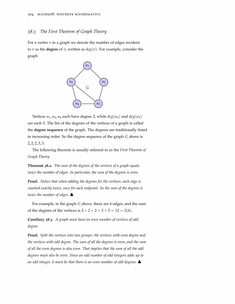
304 math208: discrete mathematics
38.3 The First Theorem of Graph Theory
For a vertex v in a graph we denote the number of edges incident
to v as the degree of v, written as deg(v). For example, consider the
graph
u5
u1
u2
u3u4
G
Vertices u1, u2, u4 each have degree 2, while deg(u3) and deg(u5)
are each 3. The list of the degrees of the vertices of a graph is called
the degree sequence of the graph. The degrees are traditionally listed
in increasing order. So the degree sequence of the graph G above is
2, 2, 2, 3, 3.
The following theorem is usually referred to as the First Theorem of
Graph Theory
Theorem 38.2. The sum of the degrees of the vertices of a graph equals
twice the number of edges. In particular, the sum of the degrees is even.
Proof. Notice that when adding the degrees for the vertices, each edge is
counted exactly twice, once for each endpoint. So the sum of the degrees is
twice the number of edges. ♣
For example, in the graph G above, there are 6 edges, and the sum
of the degrees of the vertices is 2 + 2 + 2 + 3 + 3 = 12 = 2(6).
Corollary 38.3. A graph must have an even number of vertices of odd
degree.
Proof. Split the vertices into two groups: the vertices with even degree and
the vertices with odd degree. The sum of all the degrees is even, and the sum
of all the even degrees is also even. That implies that the sum of all the odd
degrees must also be even. Since an odd number of odd integers adds up to
an odd integer, it must be that there is an even number of odd degrees. ♣
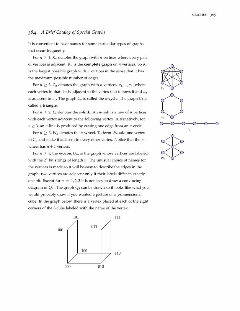
graphs 305
38.4 A Brief Catalog of Special Graphs
It is convenient to have names for some particular types of graphs
that occur frequently.
For n ≥ 1, Kn denotes the graph with n vertices where every pair
of vertices is adjacent. Kn is the complete graph on n vertices. So Kn
is the largest possible graph with n vertices in the sense that it has
the maximum possible number of edges.
K6For n ≥ 3, Cn denotes the graph with n vertices, v1, ..., vn, where
each vertex in that list is adjacent to the vertex that follows it and vn
is adjacent to v1. The graph Cn is called the n-cycle. The graph C3 is
called a triangle.
C6
For n ≥ 2, Ln denotes the n-link. An n-link is a row of n vertices
with each vertex adjacent to the following vertex. Alternatively, for
n ≥ 3, an n-link is produced by erasing one edge from an n-cycle.L6
For n ≥ 3, Wn denotes the n-wheel. To form Wn add one vertex
to Cn and make it adjacent to every other vertex. Notice that the n-
wheel has n + 1 verices.
W6
For n ≥ 1, the n-cube, Qn, is the graph whose vertices are labeled
with the 2n bit strings of length n. The unusual choice of names for
the vertices is made so it will be easy to describe the edges in the
graph: two vertices are adjacent only if their labels differ in exactly
one bit. Except for n = 1, 2, 3 it is not easy to draw a convincing
diagram of Qn. The graph Q3 can be drawn so it looks like what you
would probably draw if you wanted a picture of a 3-dimensional
cube. In the graph below, there is a vertex placed at each of the eight
corners of the 3-cube labeled with the name of the vertex.
000 010
110100
001
101 111
011
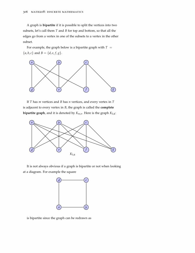
306 math208: discrete mathematics
A graph is bipartite if it is possible to split the vertices into two
subsets, let’s call them T and B for top and bottom, so that all the
edges go from a vertex in one of the subsets to a vertex in the other
subset.
For example, the graph below is a bipartite graph with T =
{a, b, c} and B = {d, e, f , g}.
a b c
d e f g
If T has m vertices and B has n vertices, and every vertex in T
is adjacent to every vertex in B, the graph is called the complete
bipartite graph, and it is denoted by Km,n. Here is the graph K3,4:
a b c
d e f gK3,4
It is not always obvious if a graph is bipartite or not when looking
at a diagram. For example the square
a b
cd
is bipartite since the graph can be redrawn as
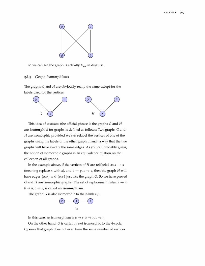
graphs 307
d b
ca
so we can see the graph is actually K2,2 in disguise.
38.5 Graph isomorphisms
The graphs G and H are obviously really the same except for the
labels used for the vertices.
a
cb
G x
zy
H
This idea of sameness (the official phrase is the graphs G and H
are isomorphic) for graphs is defined as follows: Two graphs G and
H are isomorphic provided we can relabel the vertices of one of the
graphs using the labels of the other graph in such a way that the two
graphs will have exactly the same edges. As you can probably guess,
the notion of isomorphic graphs is an equivalence relation on the
collection of all graphs.
In the example above, if the vertices of H are relabeled as a → x
(meaning replace x with a), and b → y, c → z, then the graph H will
have edges {a, b} and {a, c} just like the graph G. So we have proved
G and H are isomorphic graphs. The set of replacement rules, a → x,
b→ y, c→ z, is called an isomorphism.
The graph G is also isomorphic to the 3-link L3:
sr t
L3
In this case, an isomorphism is a→ s, b→ r, c→ t.
On the other hand, G is certainly not isomorphic to the 4-cycle,
C4 since that graph does not even have the same number of vertices
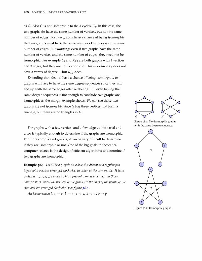
308 math208: discrete mathematics
as G. Also G is not isomorphic to the 3-cycles, C3. In this case, the
two graphs do have the same number of vertices, but not the same
number of edges. For two graphs have a chance of being isomorphic,
the two graphs must have the same number of vertices and the same
number of edges. But warning: even if two graphs have the same
number of vertices and the same number of edges, they need not be
isomorphic. For example L4 and K1,3 are both graphs with 4 vertices
and 3 edges, but they are not isomorphic. This is so since L4 does not
have a vertex of degree 3, but K1,3 does.
Extending that idea: to have a chance of being isomorphic, two
graphs will have to have the same degree sequences since they will
end up with the same edges after relabeling. But even having the
same degree sequences is not enough to conclude two graphs are
isomorphic as the margin example shows. We can see those two
graphs are not isomorphic since G has three vertices that form a
triangle, but there are no triangles in H.G H
Figure 38.1: Nonisomorphic grades
with the same degree sequences.For graphs with a few vertices and a few edges, a little trial and
error is typically enough to determine if the graphs are isomorphic.
For more complicated graphs, it can be very difficult to determine
if they are isomorphic or not. One of the big goals in theoretical
computer science is the design of efficient algorithms to determine if
two graphs are isomorphic.
e
a
b
cd
G
z
v
w
xy
H
Figure 38.2: Isomorphic graphs
Example 38.4. Let G be a 5-cycle on a, b, c, d, e drawn as a regular pen-
tagon with vertices arranged clockwise, in order, at the corners. Let H have
vertex set v, w, x, y, z and graphical presentation as a pentagram (five-
pointed star), where the vertices of the graph are the ends of the points of the
star, and are arranged clockwise, (see figure 38.2).
An isomorphism is a→ v, b→ x, c→ z, d→ w, e→ y.
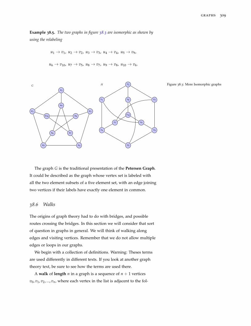
graphs 309
Example 38.5. The two graphs in figure 38.3 are isomorphic as shown by
using the relabeling
u1 → v1, u2 → v2, u3 → v3, u4 → v4, u5 → v9,
u6 → v10, u7 → v5, u8 → v7, u9 → v8, u10 → v6.
u2
u3
u4u5
u1
u9
u8
u7u6
u10
G v2
v3
v4
v5
v6
v1
v7
v8
v9
v10
H Figure 38.3: More Isomorphic graphs
The graph G is the traditional presentation of the Petersen Graph.
It could be described as the graph whose vertex set is labeled with
all the two element subsets of a five element set, with an edge joining
two vertices if their labels have exactly one element in common.
38.6 Walks
The origins of graph theory had to do with bridges, and possible
routes crossing the bridges. In this section we will consider that sort
of question in graphs in general. We will think of walking along
edges and visiting vertices. Remember that we do not allow multiple
edges or loops in our graphs.
We begin with a collection of definitions. Warning: Theses terms
are used differently in different texts. If you look at another graph
theory text, be sure to see how the terms are used there.
A walk of length n in a graph is a sequence of n + 1 vertices
v0, v1, v2, ..., vn, where each vertex in the list is adjacent to the fol-
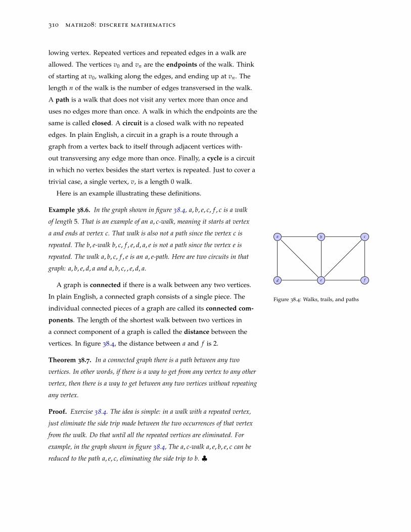
310 math208: discrete mathematics
lowing vertex. Repeated vertices and repeated edges in a walk are
allowed. The vertices v0 and vn are the endpoints of the walk. Think
of starting at v0, walking along the edges, and ending up at vn. The
length n of the walk is the number of edges transversed in the walk.
A path is a walk that does not visit any vertex more than once and
uses no edges more than once. A walk in which the endpoints are the
same is called closed. A circuit is a closed walk with no repeated
edges. In plain English, a circuit in a graph is a route through a
graph from a vertex back to itself through adjacent vertices with-
out transversing any edge more than once. Finally, a cycle is a circuit
in which no vertex besides the start vertex is repeated. Just to cover a
trivial case, a single vertex, v, is a length 0 walk.
Here is an example illustrating these definitions.
Example 38.6. In the graph shown in figure 38.4, a, b, e, c, f , c is a walk
of length 5. That is an example of an a, c-walk, meaning it starts at vertex
a and ends at vertex c. That walk is also not a path since the vertex c is
repeated. The b, e-walk b, c, f , e, d, a, e is not a path since the vertex e is
repeated. The walk a, b, c, f , e is an a, e-path. Here are two circuits in that
graph: a, b, e, d, a and a, b, c, , e, d, a.
a b c
d e f
Figure 38.4: Walks, trails, and paths
A graph is connected if there is a walk between any two vertices.
In plain English, a connected graph consists of a single piece. The
individual connected pieces of a graph are called its connected com-
ponents. The length of the shortest walk between two vertices in
a connect component of a graph is called the distance between the
vertices. In figure 38.4, the distance between a and f is 2.
Theorem 38.7. In a connected graph there is a path between any two
vertices. In other words, if there is a way to get from any vertex to any other
vertex, then there is a way to get between any two vertices without repeating
any vertex.
Proof. Exercise 38.4. The idea is simple: in a walk with a repeated vertex,
just eliminate the side trip made between the two occurrences of that vertex
from the walk. Do that until all the repeated vertices are eliminated. For
example, in the graph shown in figure 38.4, The a, c-walk a, e, b, e, c can be
reduced to the path a, e, c, eliminating the side trip to b. ♣
graphs 311
A vertex in a graph is a cutvertex, if removal of the vertex and
edges incident to it results in a graph with more connected com-
ponents. Similarly a bridge is an edge whose removal (keeping the
vertices it is incident to) yields a graph with more connected compo-
nents.
We close this section with a discussion of two special types of
walks.
38.6.1 Eulerian trails and circuits
An eulerian trail in a graph is a walk which uses every edge of the
graph exactly once. An eulerian circuit is a circuit in a graph that
uses every edge of the graph. A graph is called eulerian if it has an
eulerian circuit. An interesting property of an eulerian graph is that
it can be drawn completely without lifting pencil from paper and
without retracing any edges.
Example 38.8. The graph C5 is an eulerian graph. In fact, the graph itself
is an eulerian circuit.
Example 38.9. The graph K5 is an eulerian graph.
Example 38.10. The graph Ln is itself an eulerian trail, but does not have
an Eulerian circuit.
Example 38.11. The graph K4 is not an eulerian graph. 1. 1 Try it!
38.6.2 Hamiltonian cycles
A hamiltonian cycle in a graph is a cycle that visits every vertex
in the graph. In other words, it is a walk through the graph from
an initial vertex, visiting every vertex once, and then having a final
step back to the initial vertex. A graph is hamiltonian if it has a
hamiltonian cycle.
Example 38.12. Kn is hamiltonian for n ≥ 3.
Example 38.13. Wn has a hamiltonian cycle for n ≥ 3.
Example 38.14. Ln has no hamiltonian cycle for n ≥ 2
312 math208: discrete mathematics
38.6.3 Some facts about eulerian and hamiltonian graphs
A few easy observation: if G is a graph with either an eulerian circuit
or hamiltonian cycle, then
(1) G is connected.
(2) every vertex has degree at least 2.
(3) G has no bridges.
If G has a hamiltonian cycle, then G has no cutvertices.
Leonhard Euler gave a simple way to determine exactly when a
graph is eulerian. On the other hand, despite considerable effort, no
one has been able to devise a test to distinguish between hamiltonian
and nonhamiltonian graphs that is much better than a brute force
trial-and-error search for a hamiltonian cycle.
Theorem 38.15. A connected graph is eulerian if and only if every vertex
has even degree.
Proof. Let G be an eulerian graph, and suppose that v is a vertex in G with
odd degree, say 2m + 1. Let i denote the number of times an eulerian circuit
passes through v. Since every edge is used exactly once in the circuit, and
each time v is visited two different edges are used, we have 2i = 2m + 1,
which is impossible. →←. So G cannot have any vertices of odd degree.
Conversely, let G be a connected graph where every vertex has even
degree. Select a vertex u and build a trail starting at u as long as possible:
each time we visit a vertex we select an unused edge leaving that vertex to
extend the trail. For any vertex v 6= u we visit, its even degree guarantees
there will be an unused edge out, since each time v is visited used two edges
incident to v and one more edge to arrive at v, for a total of an odd number
of edges incident to v, and the vertex has even degree, so there must be
at least one unused edge leading out of v. Since the process of extending
the trail must eventually come to an end, that shows the end must be at u
when the trail cannot be extended, and so we have constructed an eulerian
circuit.e must reach a vertex where the trail cannot be extended. This vertex
must be u by the preceding remark.
If this trail contains every edge we are done. Otherwise when these edges
are removed from G we obtain a set of connected components H1, ..., Hm
graphs 313
which are subgraphs of G and which each satisfy that all vertices have even
degree. Since their sizes are smaller, we may inductively construct an eu-
lerian circuit for each Hi. Since each G is connected, each Hi contains a
vertex of the initial circuit, say vj. If we call the eulerian circuit of Hi, Ci,
then v0, ...vj, Ci, vj, ..., vn, v0 is a circuit in G. Since the Hi are disjoint, we
may insert each eulerian partial circuit thus obtaining an eulerian circuit for
G. ♣
As a corollary we have
Theorem 38.16. A connected graph has an eulerian trail using every edge,
if and only if it has exactly two vertices of odd degree.
The following theorem is an example of a sufficient (but not neces-
sary) condition for a graph to have a hamiltonian cycle.
Theorem 38.17. Let G be a connected graph with n ≥ 3 vertices. If
deg(v) ≥ n/2 for every vertex v, then G is hamiltonian.
Proof. Suppose that the theorem is false. Let G be a connected graph with
deg(v) ≥ n/2 for every vertex v. Moreover suppose that of all counterex-
amples on n vertices, G is a graph with the largest possible number of edges.
G is not complete, since Kn has a hamiltonian cycle, for n ≥ 3. There-
fore G has two nonadjacent vertices v1 and vn. By maximality the graph
G1 formed by adding the edge {v1, vn} to G has a hamiltonian cycle. More-
over this cycle uses the edge {v1, vn}, since otherwise G has a hamiltonian
cycle. So we may suppose that the hamiltonian cycle in G1 is of the form
v1, v2, ..., vn, v1. Thus v1, ..., vn is a path in G.
Let k = deg(v1). If vi+1 is adjacent to v1, then vi cannot be adjacent to
vn, since otherwise v1, ..., vi, vn, vn−1, ..., vi+1, v1 is a hamiltonian cycle in
G. Therefore, we have the contradiction
deg(vn) ≤ (n− 1)− k ≤ n− 1− n/2 = n/2− 1.→←
♣
WARNING: Do not read too much into this theorem. The condi-
tion is not a necessary condition. The 5-cycle, C5, is obviously hamil-
tonian, but the vertices all have degree 2 which is less than 52 .
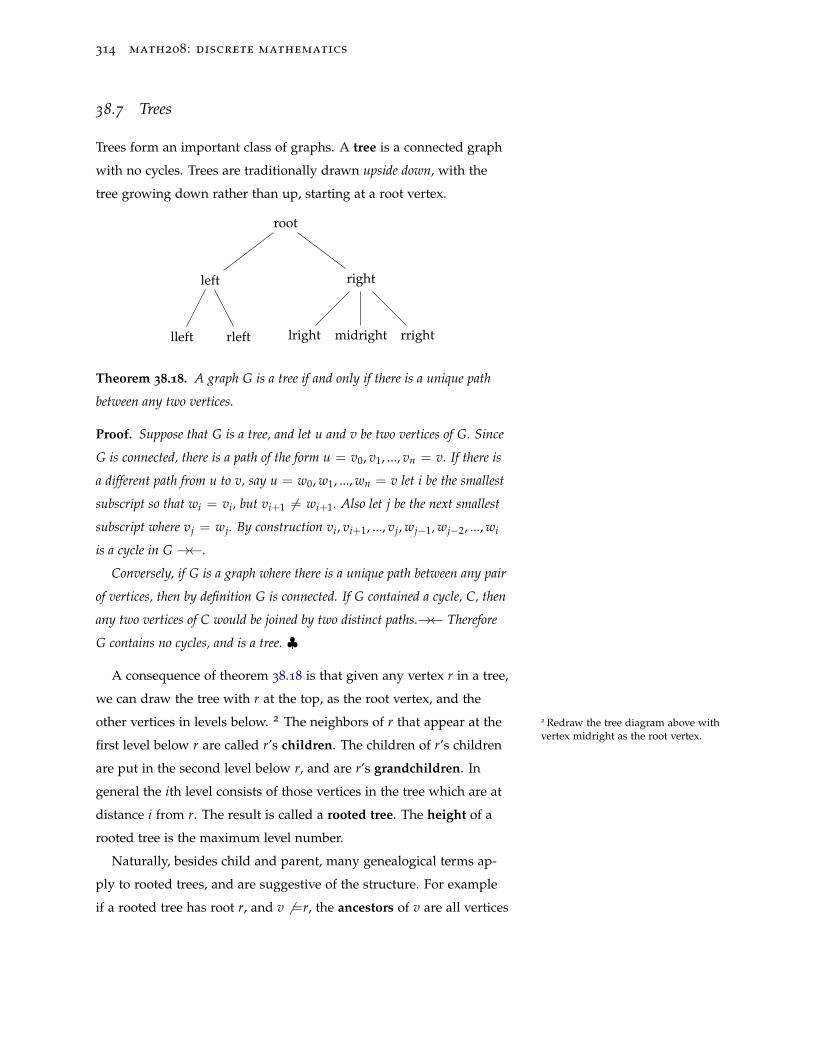
314 math208: discrete mathematics
38.7 Trees
Trees form an important class of graphs. A tree is a connected graph
with no cycles. Trees are traditionally drawn upside down, with the
tree growing down rather than up, starting at a root vertex.
root
left
lleft rleft
right
lright midright rright
Theorem 38.18. A graph G is a tree if and only if there is a unique path
between any two vertices.
Proof. Suppose that G is a tree, and let u and v be two vertices of G. Since
G is connected, there is a path of the form u = v0, v1, ..., vn = v. If there is
a different path from u to v, say u = w0, w1, ..., wn = v let i be the smallest
subscript so that wi = vi, but vi+1 6= wi+1. Also let j be the next smallest
subscript where vj = wj. By construction vi, vi+1, ..., vj, wj−1, wj−2, ..., wi
is a cycle in G→←.
Conversely, if G is a graph where there is a unique path between any pair
of vertices, then by definition G is connected. If G contained a cycle, C, then
any two vertices of C would be joined by two distinct paths.→← Therefore
G contains no cycles, and is a tree. ♣
A consequence of theorem 38.18 is that given any vertex r in a tree,
we can draw the tree with r at the top, as the root vertex, and the
other vertices in levels below. 2 The neighbors of r that appear at the 2 Redraw the tree diagram above withvertex midright as the root vertex.
first level below r are called r’s children. The children of r’s children
are put in the second level below r, and are r’s grandchildren. In
general the ith level consists of those vertices in the tree which are at
distance i from r. The result is called a rooted tree. The height of a
rooted tree is the maximum level number.
Naturally, besides child and parent, many genealogical terms ap-
ply to rooted trees, and are suggestive of the structure. For example
if a rooted tree has root r, and v 6 =r, the ancestors of v are all vertices
graphs 315
on the path from r to v, including r, but excluding v. The descen-
dants of a vertex, w consist of all vertices which have w as one of
their ancestors. The subtree rooted at w is the rooted tree consist-
ing of w, its descendants, and all the required edges. A vertex with
no children is a leaf, and a vertex with at least one child is called an
internal vertex.
To distinguish rooted trees by breadth, we use the term m-ary to
mean that any internal vertex has at most m children. An m-ary tree
is full if every internal vertex has exactly m children. When m = 2,
we use the term binary.
Theorem 38.19. A tree on n vertices has n− 1 edges.
Proof. (by induction on n.)
Basis: Let n = 1, this is the trivial tree with 0 edges. So true the theorem
is true for n = 1.
Inductive Step: Suppose that for some n ≥ 1 every tree with n vertices
has n− 1 edges. Now suppose T is a tree with n + 1 vertices. Let v be a leaf
of T. If we erase v and the edge leading to it, we are left with a tree with n
vertices. By the inductive hypothesis, this new tree will have n − 1 edges.
Since it has one less edge than the original tree, we conclude T has n edges.
♣
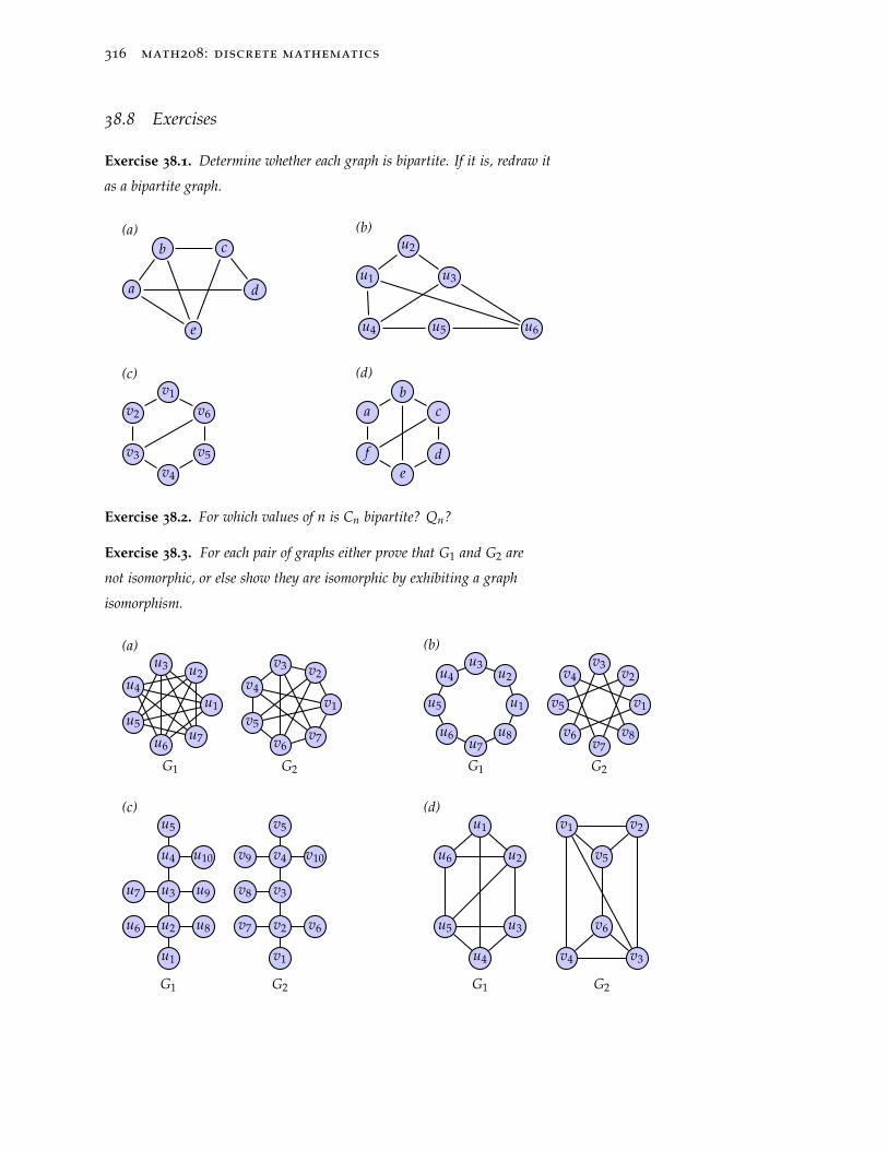
316 math208: discrete mathematics
38.8 Exercises
Exercise 38.1. Determine whether each graph is bipartite. If it is, redraw it
as a bipartite graph.
(a)
a
b c
d
e
(b)
u1
u2
u3
u5u4 u6
(c)v1
v6
v5
v4
v3
v2
(d)b
c
de
f
a
Exercise 38.2. For which values of n is Cn bipartite? Qn?
Exercise 38.3. For each pair of graphs either prove that G1 and G2 are
not isomorphic, or else show they are isomorphic by exhibiting a graph
isomorphism.
(a)
u1
u2u3
u4
u5
u6u7
G1
v1
v2v3
v4
v5
v6v7
G2
(b)
u1
u2u3
u4
u5
u6u7
u8
G1
v1
v2v3
v4
v5
v6v7
v8
G2
(c)
u1
u2
u3
u4
u5
u6
u7
u8
u9
u10
G1
v1
v2
v3
v4
v5
v7
v8
v6
v10v9
G2
(d)u1
u2
u3
u4
u5
u6
G1
v1 v2
v3v4
v5
v6
G2
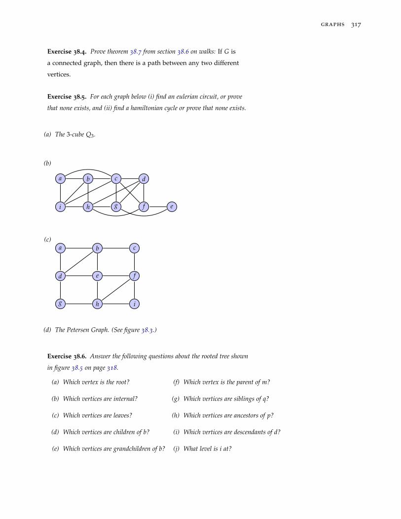
graphs 317
Exercise 38.4. Prove theorem 38.7 from section 38.6 on walks: If G is
a connected graph, then there is a path between any two different
vertices.
Exercise 38.5. For each graph below (i) find an eulerian circuit, or prove
that none exists, and (ii) find a hamiltonian cycle or prove that none exists.
(a) The 3-cube Q3.
(b)
a b c d
i h g f e
(c)a b c
d e f
g h i
(d) The Petersen Graph. (See figure 38.3.)
Exercise 38.6. Answer the following questions about the rooted tree shown
in figure 38.5 on page 318.
(a) Which vertex is the root?
(b) Which vertices are internal?
(c) Which vertices are leaves?
(d) Which vertices are children of b?
(e) Which vertices are grandchildren of b?
(f) Which vertex is the parent of m?
(g) Which vertices are siblings of q?
(h) Which vertices are ancestors of p?
(i) Which vertices are descendants of d?
(j) What level is i at?
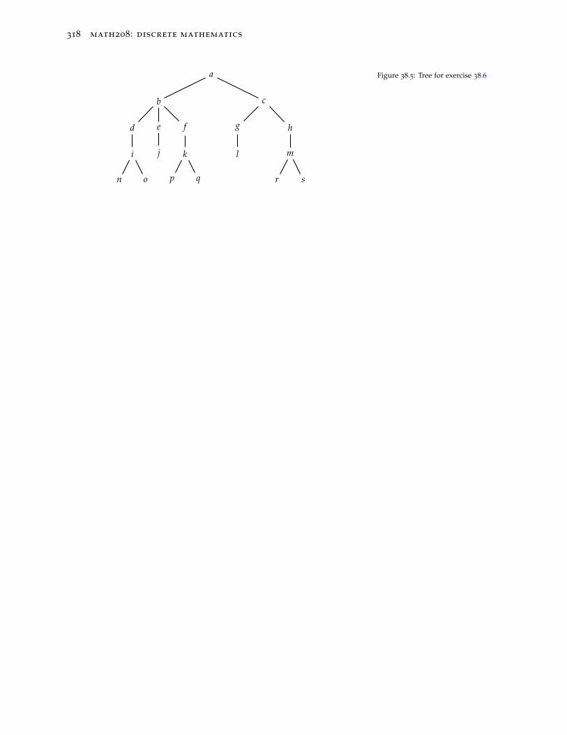
318 math208: discrete mathematics
a
b
d
i
n o
e
j
f
k
p q
c
g
l
h
m
r s
Figure 38.5: Tree for exercise 38.6
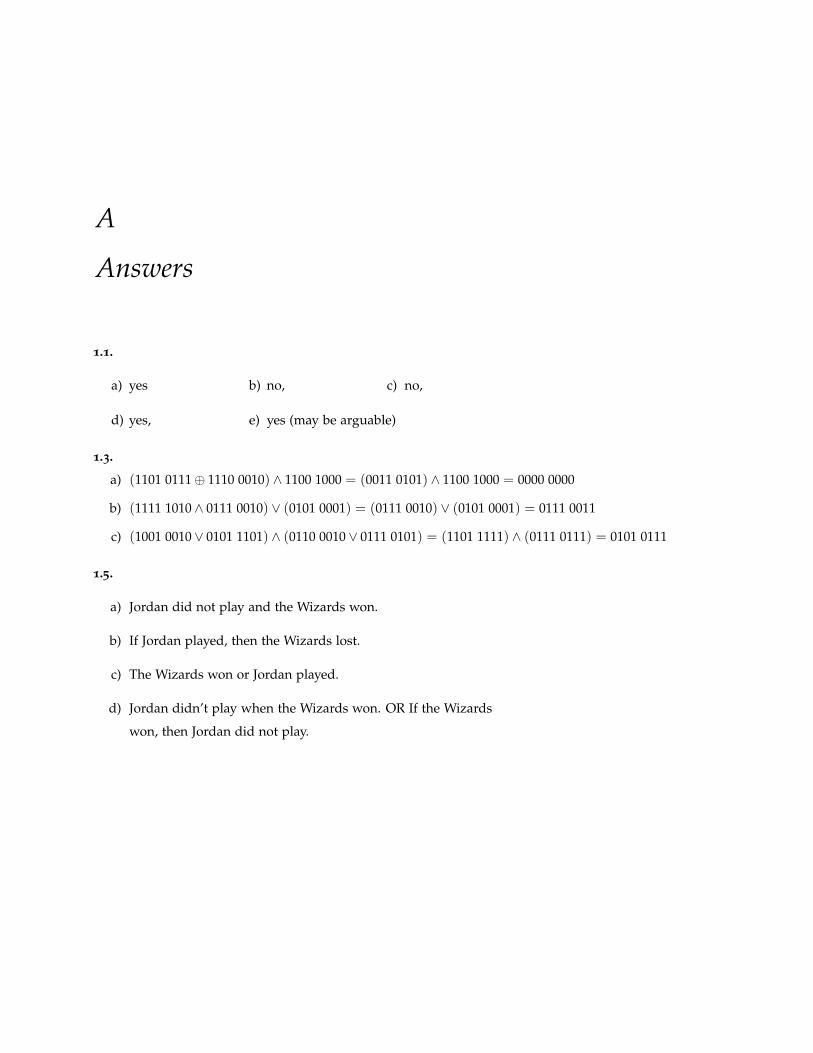
A
Answers
1.1.
yesa) no,b) no,c)
yes,d) yes (may be arguable)e)
1.3.
a) (1101 0111⊕ 1110 0010) ∧ 1100 1000 = (0011 0101) ∧ 1100 1000 = 0000 0000
b) (1111 1010∧ 0111 0010) ∨ (0101 0001) = (0111 0010) ∨ (0101 0001) = 0111 0011
c) (1001 0010∨ 0101 1101) ∧ (0110 0010∨ 0111 0101) = (1101 1111) ∧ (0111 0111) = 0101 0111
1.5.
a) Jordan did not play and the Wizards won.
b) If Jordan played, then the Wizards lost.
c) The Wizards won or Jordan played.
d) Jordan didn’t play when the Wizards won. OR If the Wizards
won, then Jordan did not play.

B
GNU Free Documentation License
Version 1.3, 3 November 2008
Copyright © 2000, 2001, 2002, 2007, 2008 Free Software Foundation,
Inc.
<http://fsf.org/>
Everyone is permitted to copy and distribute verbatim copies of this
license document, but changing it is not allowed.
Preamble
The purpose of this License is to make a manual, textbook, or
other functional and useful document “free” in the sense of freedom:
to assure everyone the effective freedom to copy and redistribute it,
with or without modifying it, either commercially or noncommer-
cially. Secondarily, this License preserves for the author and pub-
lisher a way to get credit for their work, while not being considered
responsible for modifications made by others.
This License is a kind of “copyleft”, which means that derivative
works of the document must themselves be free in the same sense.
It complements the GNU General Public License, which is a copyleft
license designed for free software.
We have designed this License in order to use it for manuals for
free software, because free software needs free documentation: a free
program should come with manuals providing the same freedoms
that the software does. But this License is not limited to software
322 math208: discrete mathematics
manuals; it can be used for any textual work, regardless of subject
matter or whether it is published as a printed book. We recommend
this License principally for works whose purpose is instruction or
reference.
1. APPLICABILITY AND DEFINITIONS
This License applies to any manual or other work, in any medium,
that contains a notice placed by the copyright holder saying it can
be distributed under the terms of this License. Such a notice grants
a world-wide, royalty-free license, unlimited in duration, to use that
work under the conditions stated herein. The “Document”, below,
refers to any such manual or work. Any member of the public is a
licensee, and is addressed as “you”. You accept the license if you
copy, modify or distribute the work in a way requiring permission
under copyright law.
A “Modified Version” of the Document means any work contain-
ing the Document or a portion of it, either copied verbatim, or with
modifications and/or translated into another language.
A “Secondary Section” is a named appendix or a front-matter
section of the Document that deals exclusively with the relationship
of the publishers or authors of the Document to the Document’s over-
all subject (or to related matters) and contains nothing that could
fall directly within that overall subject. (Thus, if the Document is in
part a textbook of mathematics, a Secondary Section may not explain
any mathematics.) The relationship could be a matter of historical
connection with the subject or with related matters, or of legal, com-
mercial, philosophical, ethical or political position regarding them.
The “Invariant Sections” are certain Secondary Sections whose
titles are designated, as being those of Invariant Sections, in the no-
tice that says that the Document is released under this License. If a
section does not fit the above definition of Secondary then it is not al-
lowed to be designated as Invariant. The Document may contain zero
Invariant Sections. If the Document does not identify any Invariant
Sections then there are none.
The “Cover Texts” are certain short passages of text that are listed,
gnu free documentation license 323
as Front-Cover Texts or Back-Cover Texts, in the notice that says that
the Document is released under this License. A Front-Cover Text may
be at most 5 words, and a Back-Cover Text may be at most 25 words.
A “Transparent” copy of the Document means a machine-readable
copy, represented in a format whose specification is available to the
general public, that is suitable for revising the document straightfor-
wardly with generic text editors or (for images composed of pixels)
generic paint programs or (for drawings) some widely available
drawing editor, and that is suitable for input to text formatters or
for automatic translation to a variety of formats suitable for input to
text formatters. A copy made in an otherwise Transparent file format
whose markup, or absence of markup, has been arranged to thwart
or discourage subsequent modification by readers is not Transpar-
ent. An image format is not Transparent if used for any substantial
amount of text. A copy that is not “Transparent” is called “Opaque”.
Examples of suitable formats for Transparent copies include
plain ASCII without markup, Texinfo input format, LaTeX input
format, SGML or XML using a publicly available DTD, and standard-
conforming simple HTML, PostScript or PDF designed for human
modification. Examples of transparent image formats include PNG,
XCF and JPG. Opaque formats include proprietary formats that can
be read and edited only by proprietary word processors, SGML or
XML for which the DTD and/or processing tools are not generally
available, and the machine-generated HTML, PostScript or PDF pro-
duced by some word processors for output purposes only.
The “Title Page” means, for a printed book, the title page itself,
plus such following pages as are needed to hold, legibly, the material
this License requires to appear in the title page. For works in formats
which do not have any title page as such, “Title Page” means the text
near the most prominent appearance of the work’s title, preceding
the beginning of the body of the text.
The “publisher” means any person or entity that distributes
copies of the Document to the public.
A section “Entitled XYZ” means a named subunit of the Docu-
ment whose title either is precisely XYZ or contains XYZ in parenthe-
324 math208: discrete mathematics
ses following text that translates XYZ in another language. (Here
XYZ stands for a specific section name mentioned below, such
as “Acknowledgements”, “Dedications”, “Endorsements”, or
“History”.) To “Preserve the Title” of such a section when you mod-
ify the Document means that it remains a section “Entitled XYZ”
according to this definition.
The Document may include Warranty Disclaimers next to the
notice which states that this License applies to the Document. These
Warranty Disclaimers are considered to be included by reference in
this License, but only as regards disclaiming warranties: any other
implication that these Warranty Disclaimers may have is void and has
no effect on the meaning of this License.
2. VERBATIM COPYING
You may copy and distribute the Document in any medium, either
commercially or noncommercially, provided that this License, the
copyright notices, and the license notice saying this License applies
to the Document are reproduced in all copies, and that you add no
other conditions whatsoever to those of this License. You may not
use technical measures to obstruct or control the reading or further
copying of the copies you make or distribute. However, you may
accept compensation in exchange for copies. If you distribute a large
enough number of copies you must also follow the conditions in
section 3.
You may also lend copies, under the same conditions stated above,
and you may publicly display copies.
3. COPYING IN QUANTITY
If you publish printed copies (or copies in media that commonly
have printed covers) of the Document, numbering more than 100, and
the Document’s license notice requires Cover Texts, you must enclose
the copies in covers that carry, clearly and legibly, all these Cover
Texts: Front-Cover Texts on the front cover, and Back-Cover Texts
on the back cover. Both covers must also clearly and legibly identify
you as the publisher of these copies. The front cover must present
gnu free documentation license 325
the full title with all words of the title equally prominent and visible.
You may add other material on the covers in addition. Copying with
changes limited to the covers, as long as they preserve the title of the
Document and satisfy these conditions, can be treated as verbatim
copying in other respects.
If the required texts for either cover are too voluminous to fit legi-
bly, you should put the first ones listed (as many as fit reasonably) on
the actual cover, and continue the rest onto adjacent pages.
If you publish or distribute Opaque copies of the Document num-
bering more than 100, you must either include a machine-readable
Transparent copy along with each Opaque copy, or state in or with
each Opaque copy a computer-network location from which the
general network-using public has access to download using public-
standard network protocols a complete Transparent copy of the
Document, free of added material. If you use the latter option, you
must take reasonably prudent steps, when you begin distribution of
Opaque copies in quantity, to ensure that this Transparent copy will
remain thus accessible at the stated location until at least one year
after the last time you distribute an Opaque copy (directly or through
your agents or retailers) of that edition to the public.
It is requested, but not required, that you contact the authors of
the Document well before redistributing any large number of copies,
to give them a chance to provide you with an updated version of the
Document.
4. MODIFICATIONS
You may copy and distribute a Modified Version of the Document
under the conditions of sections 2 and 3 above, provided that you
release the Modified Version under precisely this License, with the
Modified Version filling the role of the Document, thus licensing
distribution and modification of the Modified Version to whoever
possesses a copy of it. In addition, you must do these things in the
Modified Version:
A. Use in the Title Page (and on the covers, if any) a title distinct from
that of the Document, and from those of previous versions (which
326 math208: discrete mathematics
should, if there were any, be listed in the History section of the
Document). You may use the same title as a previous version if the
original publisher of that version gives permission.
B. List on the Title Page, as authors, one or more persons or entities
responsible for authorship of the modifications in the Modified
Version, together with at least five of the principal authors of the
Document (all of its principal authors, if it has fewer than five),
unless they release you from this requirement.
C. State on the Title page the name of the publisher of the Modified
Version, as the publisher.
D. Preserve all the copyright notices of the Document.
E. Add an appropriate copyright notice for your modifications adja-
cent to the other copyright notices.
F. Include, immediately after the copyright notices, a license notice
giving the public permission to use the Modified Version under
the terms of this License, in the form shown in the Addendum
below.
G. Preserve in that license notice the full lists of Invariant Sections
and required Cover Texts given in the Document’s license notice.
H. Include an unaltered copy of this License.
I. Preserve the section Entitled “History”, Preserve its Title, and
add to it an item stating at least the title, year, new authors, and
publisher of the Modified Version as given on the Title Page. If
there is no section Entitled “History” in the Document, create one
stating the title, year, authors, and publisher of the Document as
given on its Title Page, then add an item describing the Modified
Version as stated in the previous sentence.
J. Preserve the network location, if any, given in the Document for
public access to a Transparent copy of the Document, and likewise
the network locations given in the Document for previous versions
it was based on. These may be placed in the “History” section.
gnu free documentation license 327
You may omit a network location for a work that was published
at least four years before the Document itself, or if the original
publisher of the version it refers to gives permission.
K. For any section Entitled “Acknowledgements” or “Dedications”,
Preserve the Title of the section, and preserve in the section all the
substance and tone of each of the contributor acknowledgements
and/or dedications given therein.
L. Preserve all the Invariant Sections of the Document, unaltered in
their text and in their titles. Section numbers or the equivalent are
not considered part of the section titles.
M. Delete any section Entitled “Endorsements”. Such a section may
not be included in the Modified Version.
N. Do not retitle any existing section to be Entitled “Endorsements”
or to conflict in title with any Invariant Section.
O. Preserve any Warranty Disclaimers.
If the Modified Version includes new front-matter sections or ap-
pendices that qualify as Secondary Sections and contain no material
copied from the Document, you may at your option designate some
or all of these sections as invariant. To do this, add their titles to the
list of Invariant Sections in the Modified Version’s license notice.
These titles must be distinct from any other section titles.
You may add a section Entitled “Endorsements”, provided it con-
tains nothing but endorsements of your Modified Version by various
parties—for example, statements of peer review or that the text has
been approved by an organization as the authoritative definition of a
standard.
You may add a passage of up to five words as a Front-Cover Text,
and a passage of up to 25 words as a Back-Cover Text, to the end of
the list of Cover Texts in the Modified Version. Only one passage of
Front-Cover Text and one of Back-Cover Text may be added by (or
through arrangements made by) any one entity. If the Document
already includes a cover text for the same cover, previously added
by you or by arrangement made by the same entity you are acting on
328 math208: discrete mathematics
behalf of, you may not add another; but you may replace the old one,
on explicit permission from the previous publisher that added the
old one.
The author(s) and publisher(s) of the Document do not by this
License give permission to use their names for publicity for or to
assert or imply endorsement of any Modified Version.
5. COMBINING DOCUMENTS
You may combine the Document with other documents released
under this License, under the terms defined in section 4 above for
modified versions, provided that you include in the combination all
of the Invariant Sections of all of the original documents, unmodified,
and list them all as Invariant Sections of your combined work in its
license notice, and that you preserve all their Warranty Disclaimers.
The combined work need only contain one copy of this License,
and multiple identical Invariant Sections may be replaced with a sin-
gle copy. If there are multiple Invariant Sections with the same name
but different contents, make the title of each such section unique by
adding at the end of it, in parentheses, the name of the original au-
thor or publisher of that section if known, or else a unique number.
Make the same adjustment to the section titles in the list of Invariant
Sections in the license notice of the combined work.
In the combination, you must combine any sections Entitled “His-
tory” in the various original documents, forming one section Entitled
“History”; likewise combine any sections Entitled “Acknowledge-
ments”, and any sections Entitled “Dedications”. You must delete all
sections Entitled “Endorsements”.
6. COLLECTIONS OF DOCUMENTS
You may make a collection consisting of the Document and other
documents released under this License, and replace the individual
copies of this License in the various documents with a single copy
that is included in the collection, provided that you follow the rules
of this License for verbatim copying of each of the documents in all
other respects.
gnu free documentation license 329
You may extract a single document from such a collection, and dis-
tribute it individually under this License, provided you insert a copy
of this License into the extracted document, and follow this License
in all other respects regarding verbatim copying of that document.
7. AGGREGATION WITH INDEPENDENT WORKS
A compilation of the Document or its derivatives with other sep-
arate and independent documents or works, in or on a volume of a
storage or distribution medium, is called an “aggregate” if the copy-
right resulting from the compilation is not used to limit the legal
rights of the compilation’s users beyond what the individual works
permit. When the Document is included in an aggregate, this License
does not apply to the other works in the aggregate which are not
themselves derivative works of the Document.
If the Cover Text requirement of section 3 is applicable to these
copies of the Document, then if the Document is less than one half
of the entire aggregate, the Document’s Cover Texts may be placed
on covers that bracket the Document within the aggregate, or the
electronic equivalent of covers if the Document is in electronic form.
Otherwise they must appear on printed covers that bracket the whole
aggregate.
8. TRANSLATION
Translation is considered a kind of modification, so you may dis-
tribute translations of the Document under the terms of section 4.
Replacing Invariant Sections with translations requires special per-
mission from their copyright holders, but you may include trans-
lations of some or all Invariant Sections in addition to the original
versions of these Invariant Sections. You may include a translation
of this License, and all the license notices in the Document, and any
Warranty Disclaimers, provided that you also include the original En-
glish version of this License and the original versions of those notices
and disclaimers. In case of a disagreement between the translation
and the original version of this License or a notice or disclaimer, the
original version will prevail.
330 math208: discrete mathematics
If a section in the Document is Entitled “Acknowledgements”,
“Dedications”, or “History”, the requirement (section 4) to Preserve
its Title (section 1) will typically require changing the actual title.
9. TERMINATION
You may not copy, modify, sublicense, or distribute the Document
except as expressly provided under this License. Any attempt oth-
erwise to copy, modify, sublicense, or distribute it is void, and will
automatically terminate your rights under this License.
However, if you cease all violation of this License, then your li-
cense from a particular copyright holder is reinstated (a) provision-
ally, unless and until the copyright holder explicitly and finally termi-
nates your license, and (b) permanently, if the copyright holder fails
to notify you of the violation by some reasonable means prior to 60
days after the cessation.
Moreover, your license from a particular copyright holder is re-
instated permanently if the copyright holder notifies you of the
violation by some reasonable means, this is the first time you have
received notice of violation of this License (for any work) from that
copyright holder, and you cure the violation prior to 30 days after
your receipt of the notice.
Termination of your rights under this section does not terminate
the licenses of parties who have received copies or rights from you
under this License. If your rights have been terminated and not per-
manently reinstated, receipt of a copy of some or all of the same
material does not give you any rights to use it.
10. FUTURE REVISIONS OF THIS LICENSE
The Free Software Foundation may publish new, revised versions
of the GNU Free Documentation License from time to time. Such
new versions will be similar in spirit to the present version, but may
differ in detail to address new problems or concerns. See http://www.gnu.org/copyleft/.
Each version of the License is given a distinguishing version num-
ber. If the Document specifies that a particular numbered version of
this License “or any later version” applies to it, you have the option
gnu free documentation license 331
of following the terms and conditions either of that specified ver-
sion or of any later version that has been published (not as a draft)
by the Free Software Foundation. If the Document does not specify
a version number of this License, you may choose any version ever
published (not as a draft) by the Free Software Foundation. If the
Document specifies that a proxy can decide which future versions of
this License can be used, that proxy’s public statement of acceptance
of a version permanently authorizes you to choose that version for
the Document.
11. RELICENSING
“Massive Multiauthor Collaboration Site” (or “MMC Site”) means
any World Wide Web server that publishes copyrightable works and
also provides prominent facilities for anybody to edit those works.
A public wiki that anybody can edit is an example of such a server.
A “Massive Multiauthor Collaboration” (or “MMC”) contained in
the site means any set of copyrightable works thus published on the
MMC site.
“CC-BY-SA” means the Creative Commons Attribution-Share Alike
3.0 license published by Creative Commons Corporation, a not-for-
profit corporation with a principal place of business in San Francisco,
California, as well as future copyleft versions of that license pub-
lished by that same organization.
“Incorporate” means to publish or republish a Document, in
whole or in part, as part of another Document.
An MMC is “eligible for relicensing” if it is licensed under this
License, and if all works that were first published under this License
somewhere other than this MMC, and subsequently incorporated in
whole or in part into the MMC, (1) had no cover texts or invariant
sections, and (2) were thus incorporated prior to November 1, 2008.
The operator of an MMC Site may republish an MMC contained in
the site under CC-BY-SA on the same site at any time before August
1, 2009, provided the MMC is eligible for relicensing.
ADDENDUM: How to use this License for your
documents
332 math208: discrete mathematics
To use this License in a document you have written, include a copy
of the License in the document and put the following copyright and
license notices just after the title page:
Copyright © YEAR YOUR NAME. Permission is granted to copy,
distribute and/or modify this document under the terms of the GNU
Free Documentation License, Version 1.3 or any later version published
by the Free Software Foundation; with no Invariant Sections, no Front-
Cover Texts, and no Back-Cover Texts. A copy of the license is included
in the section entitled “GNU Free Documentation License”.
If you have Invariant Sections, Front-Cover Texts and Back-Cover
Texts, replace the “with . . . Texts.” line with this:
with the Invariant Sections being LIST THEIR TITLES, with the Front-
Cover Texts being LIST, and with the Back-Cover Texts being LIST.
If you have Invariant Sections without Cover Texts, or some other
combination of the three, merge those two alternatives to suit the
situation.
If your document contains nontrivial examples of program code,
we recommend releasing these examples in parallel under your
choice of free software license, such as the GNU General Public Li-
cense, to permit their use in free software.