math 7890, utah spring 2017: introduction to the …patrikis/7890spring2017/allnotes.pdf · math...
TRANSCRIPT
MATH 7890, UTAH SPRING 2017: INTRODUCTION TO THEGEOMETRIC SATAKE CORRESPONDENCE
1. Overview (notes by Michael Zhao) 21.1. Next Few Weeks 21.2. Course Overview 22. Representation and Structure Theory of Compact Lie Groups (notes by Michael
Zhao) 32.1. Lie Algebras 42.2. Exponential Map 42.3. Representation of Compact Lie Groups 52.4. Onto Representation Theory 62.5. The Representation Ring 83. Algebraic Groups (Adam Brown) 103.1. Functorial Perspective 103.2. Representations of Algebraic Groups 113.3. Maximal Tori 133.4. Representations of Tori 133.5. Structure Theory of Reductive Groups over k = k 144. Flag Varieties (Notes by Anna Romanova) 195. The Functor of Points Perspective 206. The Geometric Perspective 227. The Bruhat Decomposition 248. Borel-Weil Theorem and Theorem of highest weight (notes by Allechar Serrano
Lopez) 279. Proof of the Theorem (notes by Sean McAffee) 3010. Tannakian Categories: definitions and motivation (notes by Christian Klevdal) 3410.1. Homological Motives 3511. The main theorem of neutral Tannakian categories (notes by Shiang Tang) 3712. p-adic Groups (notes by Kevin Childers) 4012.1. Introduction 4012.2. Representations of GLn(Fp) 4112.3. Locally profinite groups 4212.4. The induction functor 4312.5. Representation theory of reductive groups over local fields 4413. Studying K-spherical representations via Hecke algebras (Notes by Sabine Lang) 4513.1. Overview of the translation from smooth G-representations to smooth
H(G)-modules 4613.2. Relation between left and right Haar measures 4713.3. Back to Hecke algebras 4913.4. Construction of the equivalence M(G)→ { smooth H(G)−modules} 5013.5. A couple of loose ends 5114. Statement of classical Satake isomorphism 5215. Sketch of proof of the Satake isomorphism (Christian Klevdal) 56
1
2MATH 7890, UTAH SPRING 2017: INTRODUCTION TO THE GEOMETRIC SATAKE CORRESPONDENCE
16. Function sheaf dictionary 6017. Introduction to Affine Grassmanians (Notes by Marin Petkovic) 6317.1. The affine Grassmannian of GLn 6317.2. Affine Grassmanian for general groups 6517.3. Another description of GrG 6718. Review of homological algebra (Allechar Serrano Lopez) 6918.1. Topological analogue 7018.2. The construction of D(C) 7618.3. Truncation structure on D(C) and t-structures 7819. Derived Functors (notes by Michael Zhao) 8319.1. Construction of Derived Functors 8320. Sheaf Cohomology (notes by Michael Zhao) 8620.1. Internal Hom 8721. Perverse Sheaves (Christian Klevdal) 8822. t-structures and gluing (Notes by Sabine Lang) 9422.1. How to make perverse sheaves ? 9722.2. Some preliminaries 9723. Intermediate extension (Allechar Serrano Lopez) 9924. Examples. Poincare Duality. 10125. Statements of a few more basic facts about perverse sheaves in algebraic
geometry 105References 106
Contents
1. Overview (notes by Michael Zhao)
1.1. Next Few Weeks. Over the next few weeks, we will cover
1. compact groups,
2. basics of algebraic groups,
3. Flag varieties and Bruhat decomposition,
4. Highest weight theory and Borel-Weil theorem,
5. Tannakian categories.
The next unit will start with the smooth representations of reductive groups over local fields.
1.2. Course Overview. Our goal is to get to the geometric Satake equivalence. Let kbe an algebraically closed field. Let G be a connected reductive algebraic group over k(e.g. GLn(k), SLn(k), Sp2n(k), G2). The geometric Satake equivalence says there is theequivalence of abelian tensor (!) categories
Perv“G(k[[t]])”
(“G(k((t)))
/G(k[[t]])”
)∼−− Rep(G∨).
The left-hand side is the category of perverse sheaves on GrG, the affine Grassmannian ofG, and the right-hand the category of finite dimensional algebraic representations of the
MATH 7890, UTAH SPRING 2017: INTRODUCTION TO THE GEOMETRIC SATAKE CORRESPONDENCE3
Langlands dual group of G (e.g if G = GLn(k), G∨ = G, and if G = Sp2n(k), G∨ =SO2n+1(k)).
1.2.1. Part I of the Class. Understand Rep(G∨).
1.2.2. Part II of the Class. The classical Satake isomorphism and smooth representations ofreductive groups over local fields. It is the isomorphism
C∞c,“G(k[[t]])”
(“G(k((t)))
/G(k[[t]])”
)∼−→ R(G∨),
obtained by taking the Grothendieck group of both sides (applying K0) of the geometricSatake equivalence. The left-hand side is called the spherical Hecke algebra of G, whicharises from studying the smooth representations of G(k((t))) or G(Qp), and is made into analgebra by convolution of functions. The right-hand side is the representation ring of theLanglands dual of G.
1.2.3. Part III of the Class. Understand the Perv of the geometric Satake equivalence. Thisentails understanding the six operations (e.g. f∗, f
∗) on derived categories of (constructible)sheaves on algebraic varieties, and the full subcategory of perverse sheaves.
1.2.4. Part IV of the Class. This will be distributed throughout the course, but the goal isto understand what GrG is.
1.2.5. Part V of the Class. The geometric Satake equivalence.
2. Representation and Structure Theory of Compact Lie Groups (notes byMichael Zhao)
Definition 2.1. A Lie group is a group object in the category of smooth manifolds, i.e.m : G×G→ G, inv : G→ G, id : 1→ G, satisfying the expected commutative diagrams.
Example 2.2. The following are Lie groups.
• GLn(R) ⊂Mn(R) ' Rn2
• Sp2n(R) = {g ∈ SL2n(R) | g preserves a non-degenerate alternating form}
• More generally, closed subgroups G ↪−→ GLn(R).
• Unipotent matrices, invertible upper triangular matrices (Borel subgroup).
• SL2(R). π1(SL2(R)) ' Z. This can be established by looking at the Iwasawa decom-position of SL2(R). The covering space corresponding to 2Z ⊂ π1(SL2(R)) is denoted
by SL2(R), and called the metaplectic cover of SL2(R). It is a Lie group but can’tbe embedded into GLn(R).
The metaplectic group is not relevant for us.
4MATH 7890, UTAH SPRING 2017: INTRODUCTION TO THE GEOMETRIC SATAKE CORRESPONDENCE
2.1. Lie Algebras. The Lie algebra g of G is given by the tangent space at the identity.It is a priori a vector space, but the Lie bracket gives it an algebra structure, which we willdescribe briefly.
There is a map Ψ : G → Aut(G) since G acts on G by conjugation. Since Ψ(g) preservesthe identity, we can look at the map
Ad : G→ AutR(g),
given by
g → dΨ(g)∣∣1.
By differentiating at the identity, we obtain the map
ad : g→ EndR(g).
Then we can define the Lie bracket as [X, Y ] := ad(X)(Y ).
Example 2.3. For G = GLn(R), g = Mn(R), and [X, Y ] = XY − Y X.
2.2. Exponential Map. Here we will explain the role of Lie algebras, by constructing amap exp : g→ G. For G = GLn(k), exp(X) =
∑nX
n/n!.
2.2.1. exp Facts. Before giving the construction, note several facts.
1. exp is a local diffeomorphism near 0, by the implicit function theorem.
2. exp is not a homomorphism once G is non-abelian.
2.2.2. exp Construction. Take X ∈ g. Use left-multiplication to propagate X to a left-invariant vector field ξX on G, i.e. ξX(g) = (mg)∗(X).
Construct an integral curve ϕX for this vector field by the following procedure. Solve thedifferential equation ψ(0) = 1, ψ′X(t) = ξX(ψX(t)). This gives a function ψX : (−ε, ε)→ G.
Note that ψX is a homomorphism. Fix s and let t vary. Let α(t) = ψX(s)ψX(t) and letβ(t) = ψX(s + t). Then α(0) = β(0), and α′(t) = ξX(α(t)) and β′(t) = ξX(β(t)) by left-invariance of ξX . Thus, α = β.
This can be extended to a homomorphism ϕX : R → G, by setting ϕX(t) = φX(t/N)N ,where N is an integer such that t/N < ε/2. This does not depend on the choice of N ; if Mwas another such integer, we would have
ψX
(t
MN
)N= ψX
(t
M
), ψX
(t
MN
)M= ψX
(t
N
).
Hence
ψX
(t
M
)M= φX
(t
MN
)MN
= φX
(t
N
)N.
Using this definition and the fact that ϕX is a homomorphism in (−ε, ε), it can be shownϕX is a homomorphism R→ G.
Definition 2.4. expG(X) := ϕX(1).
MATH 7890, UTAH SPRING 2017: INTRODUCTION TO THE GEOMETRIC SATAKE CORRESPONDENCE5
Remark 2.5. For G a compact connected Lie group, g its Lie algebra, expG : g → G issurjective. The basic idea of the proof is to use the Killing form on a Lie algebra. Usemultiplication to transport it to a Riemannian metric. The integral curves are geodesics,and any two points are connected by a geodesic.
Exercise 2.6. Find a G where expG is not surjective.
We do not need to look far for such an example. If G = GL2(R), and λ1, λ2 are two distinctnegative real numbers, consider
B =
(λ1 00 λ2
).
If there is an A ∈ Mn(R) with exp(A) = B, and A has eigenvalues α1, α2, then eαi = λi.Since λi are negative, α1 and α2 are complex conjugates. Thus λ1, λ2 have the same absolutevalue, a contradiction.
2.3. Representation of Compact Lie Groups.
Definition 2.7. A representation of G a compact Lie group is a continuous (hence smooth)homomorphism G→ GLn(C).
The motto here is to study representations of G by restricting to a maximal tori.
Definition 2.8. A (compact) torus is a (compact) connected abelian Lie group.
Example 2.9. S1 is a torus, and all compact examples are isomorphic to (S1)n.
Definition 2.10. A character (or weight) of T is a continuous homomorphism T → S1.Write X•(T ) for the abelian group of characters of T .
Exercise 2.11. Prove the following lemma.
Lemma 2.12. If T ' Rn/Zn, then all characters of T have the form
(x1, ..., xn)→n∏r=1
e2πiarxr ,
where all ar ∈ Z.
Proof. We just need to know what homomorphisms there are from R/Z to S1 (viewed as theunit circle in C). This is the same as knowing the homomorphisms from R/Z → R/Z, andany such ϕ lifts to a homomorphism φ from R to R, by using twice the fact that a universalcovering space covers any connected cover.
This construction shows φ(1) ≡ 0 (mod 1), so for some integer n, φ(1) = n, φ(a) = na,bφ(a/b) = φ(a) = na. By continuity, φ(x) = nx for any x. Then ϕ(x) = φ(x) = nx (mod 1).As x → e2πix is a homeomorphism R/Z → S1, any homomorphism R/Z → S1 is given byx→ e2πinx, for some n. �
Lemma 2.13. Any compact torus has a (dense set of) topological generators, i.e. there is
t ∈ T with T = 〈t〉.
Proof. Assume T ' Rn/Zn, and take T 3 t = (t1, ..., tn). Let H := 〈t〉. Then use the
6MATH 7890, UTAH SPRING 2017: INTRODUCTION TO THE GEOMETRIC SATAKE CORRESPONDENCE
Lemma 2.14. H = T if and only if 1, t1, ..., tn are Q-linearly independent.
If H 6= T , then T/H, a compact torus, has a non-trivial character χ, and
χ(x1, ..., xn) =∏r
e2πiarxr ,
for some integers ar not all zero. Then χ∣∣H
= 1 if and only if χ(t) = 1 if and only if∑artr ∈ Z, which implies 1, t1, ..., tn are Q-linearly dependent. �
Theorem 2.15. Let G be a compact connected Lie group. Fix a maximal torus T ⊂ G.
(1) Every g ∈ G is conjugate to an element of T .
(2) Any other maximal torus T ′ ⊂ G is G-conjugate to T .
(3) CG(T ) = T .
Exercise 2.16. Find a counter-example for non-compact groups. We already know (1) forU(n). Why?
An example of a non-compact Lie group without any tori is Rn. A maximal torus of U(n) isthe subgroup of all diagonal matrices. The spectral theorem tells us that any unitary matrixcan be diagonalized by another unitary matrix gives (1) for U(n).
Proof. Idea of the proof:
(1) follows from surjectivity of expG.
(2) is immediate from (1).
(3) uses surjectivity of expG.
�
2.4. Onto Representation Theory. Let G be a compact connected group as before.
Proposition 2.17. Any finite dimensional representation of G is isomorphic to a direct sumof irreducible representations.
Proof. The proof is the same as in the finite case. Let V ∈ Rep(G). Fix a hermitian innerproduct ( , ) on V . Produce a G-invariant inner product 〈 , 〉 by using the Haar measurethat exists on G:
〈v, w〉 =
∫G
(g · v, g · w) dg.
If W is a G-subrepresentation of V , then V decomposes as V = W ⊕W⊥ (W⊥ is G-stablesince 〈 , 〉 is G-invariant. �
The following is due to Schur.
Corollary 2.18. If V is irreducible, then EndC[G](V ) = C.
MATH 7890, UTAH SPRING 2017: INTRODUCTION TO THE GEOMETRIC SATAKE CORRESPONDENCE7
Proof. Let T ∈ EndC[G](V ). Since V is finite-dimensional, T has an eigenvalue λ. Then ifT is non-constant, T − λ · 1 acts on V and satisfies 0 6= ker(T − λ · 1) ⊂ V . Since V isirreducible, ker(T − λ · 1) = V , so T = λ. �
Definition 2.19. Let V ∈ Rep(G). The character χV of V is a homomorphism G → Cgiven by g → tr(g
∣∣V
).
Some basic facts about characters.
1. χV only depends on the isomorphism class of V .
2. χV only depends on the conjugacy class of its argument.
3. χV⊕W = χV + χW .
4. χV⊗W = χV χW .
5. χV ∗ = χV , where V = Hom(V,C).
The first four properties give us a homomorphism K0(Rep(G)) = R(G) → C(G). ViewingχV in L2(G) with an inner product
〈f1, f2〉 =
∫G
f1(g)f2(g) dg,
we have the following basic calculation.
Proposition 2.20. (1) For V,W ∈ Rep(G), 〈χV , χW 〉 = dim HomG(V,W ).
(2) Characters of irreducible representations are orthnormal (Schur).
(3) χV = χW if and only if V ' W .
Proof. Prior to describing a sketch of the proof, we will need the following two lemmas (leftas exercises).
Lemma 2.21. For all V ∈ Rep(G), dimV G =
∫G
χV (g) dg.
Proof. Let ρ be the map G → GLn(V ) associated to V . Recall that there exists a uniquelinear transformation A such that for any f ∈ V ∗,∫
G
f(ρ(g)v) dg = f(Av),
and that the action of∫Gρ(g) dg is defined to be the action of A. We will show that
imA = V G and that A is a projection operator. Since the trace of a projection operator andits rank coincide, this will prove the lemma.
Due to left-invariance of Haar measure and this fact, we can prove
ρ(h)
∫G
ρ(g) dg =
∫G
ρ(h)ρ(g) dg =
∫G
ρ(hg) dg =
∫G
ρ(g) dg,
when viewed as operators on V . For instance, the first equality follows from the fact thatfor any linear form f , f ◦ ρ(h) is also a linear form. This lets us prove that ρ(h)Av = Av forA =
∫Gρ(g) dg. Hence imA ⊂ V G. Now suppose we have v such that ρ(g) · v = v for every
8MATH 7890, UTAH SPRING 2017: INTRODUCTION TO THE GEOMETRIC SATAKE CORRESPONDENCE
g ∈ G. Then for any f ∈ V ∗, f(ρ(g) · v) = f(v). Taking the integral over G, f(Av) = f(v).On V G, then, A acts as the identity. From this, surjectivity and idempotency follow. �
Lemma 2.22. For all V , the natural map⊕W
W ⊗ HomG(W,V )→ V,
where the sum is taken over all irreducible representations W , given by
w ⊗ ϕ→ ϕ(w),
is an isomorphism of G-representations (the action of G on HomG(W,V ) is trivial).
Proof. Since W is irreducible, any element of HomG(W,V ) is an embedding. Since Rep(G)is semi-simple, the dimension of HomG(W,V ) counts the multiplicitly of W in V . Then itsuffices to show that for every irreducible W ,
W ⊗ HomG(W,V ) ' W d,
where d := dim HomG(W,V ). Taking a basis of HomG(W,V ) gives an identification withCd, and provides the isomorphism. �
Then we can calculate
dim HomG(V,W ) = dim(V ∗ ⊗W )G
2.21=
∫G
χV ∗⊗W (g) dg
=
∫G
χV (g) · χW (g) dg
= 〈χV , χW 〉,
which proves (1). Part (2) is proven by using (1) and Schur’s Lemma. For part (3), uselemma 2.22, with part (1). If χV1 = χV2 , then for all irreducible W , dim HomG(W,Vi) is thesame for i = 1, 2. Then apply the lemma. �
Proposition 2.23. Let T < G be a maximal torus. Then V,W ∈ Rep(G) are isomorphic ifand only if V
∣∣T' W
∣∣T
.
Proof. If V∣∣T' W
∣∣T
, then χV∣∣T
= χW∣∣T
. Since characters are invariant under conjugation,and the union of the conjugates of T is G, χV = χW on all of G, hence V ' W . �
This justifies the motto we had earlier, that to study representations of G we can restrictour attention to a maximal torus.
2.5. The Representation Ring. We can rephrase proposition 2.23; recall that
R(G) = K0(Rep(G)).
MATH 7890, UTAH SPRING 2017: INTRODUCTION TO THE GEOMETRIC SATAKE CORRESPONDENCE9
Proposition 2.24. The restriction map res : R(G)→ R(T ) given by
R(G) 3 V → V∣∣T
=⊕
λ∈X•(T )
Vλ (= {v ∈ V |t · v = λ(t)v, ∀t ∈ T})
is injective.
Thus to classify representations of G, we can just identify the image. Moreover, there is asymmetry present in the image of this map.
2.5.1. Weyl Group. That symmetry is related to the Weyl group.
Definition 2.25. Let NG(T ) be the normalizer of T in G. The Weyl group W (G, T ) :=NG(T )/T . Often we will just write W , as this group doesn’t depend on the choice of T , upto isomorphism.
Remark 2.26. Note that W is a finite group. Note that NG(T ) is closed, hence a compactsubgroup. Also, expT induces an isomorphism of T with Lie(T ) modulo some lattice Λ. Wacts faithfully on this lattice, i.e. we have an embedding
W ↪−→ AutZ(Λ),
so W is both compact and discrete, hence finite.
Example 2.27. If G = SU(n), then W ' Sn (think permutation matrices).
The action of W on T induces an action of W on X•(T ), given byωχ(t) = χ(ω−1 · t).
Hence res(R(G)) lands in Z[X•(T )]W ⊂ Z[X•(T )], because characters are conjugacy invari-ant.
Theorem (of the Highest Weight).
res : R(G) ' Z[X•(T )]W
Later, we’ll prove this in the setting of reductive algebraic groups.
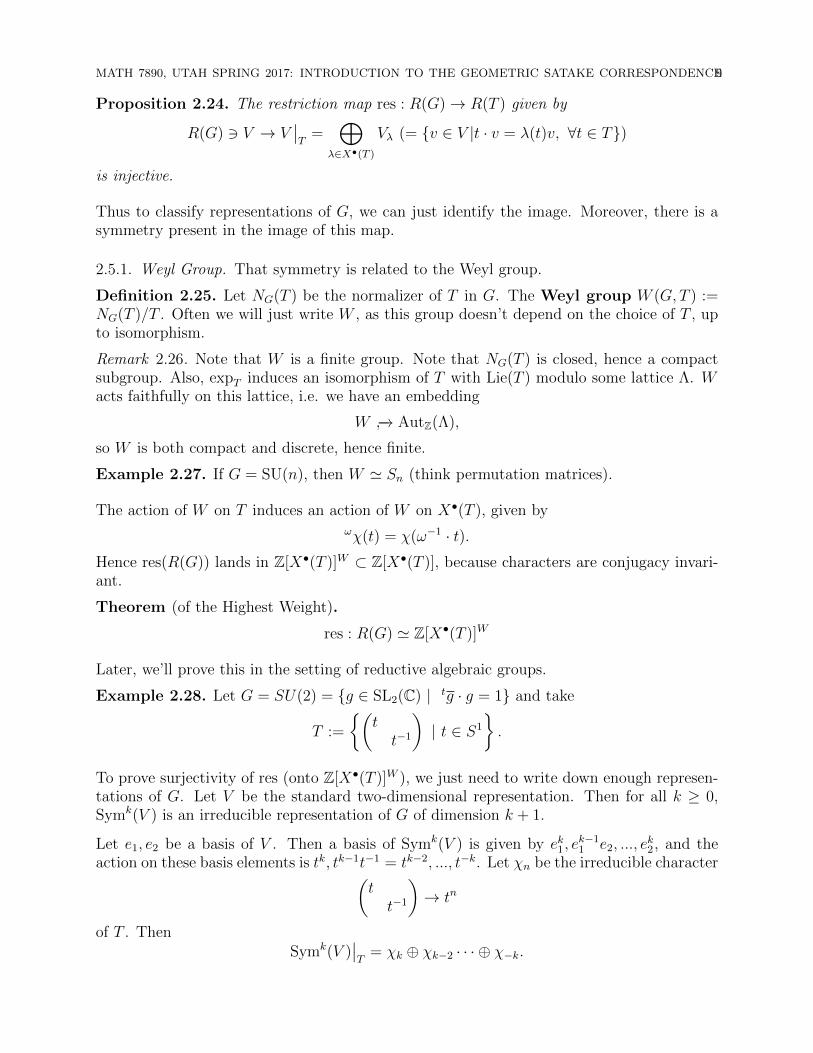
Example 2.28. Let G = SU(2) = {g ∈ SL2(C) | tg · g = 1} and take
T :=
{(tt−1
)| t ∈ S1
}.
To prove surjectivity of res (onto Z[X•(T )]W ), we just need to write down enough represen-tations of G. Let V be the standard two-dimensional representation. Then for all k ≥ 0,Symk(V ) is an irreducible representation of G of dimension k + 1.
Let e1, e2 be a basis of V . Then a basis of Symk(V ) is given by ek1, ek−11 e2, ..., e
k2, and the
action on these basis elements is tk, tk−1t−1 = tk−2, ..., t−k. Let χn be the irreducible character(tt−1
)→ tn
of T . ThenSymk(V )
∣∣T
= χk ⊕ χk−2 · · · ⊕ χ−k.
10MATH 7890, UTAH SPRING 2017: INTRODUCTION TO THE GEOMETRIC SATAKE CORRESPONDENCE
Note that if ω ∈ W \ {1}, then ωχk = χ−k, because(1
−1
)(tt−1
)(−1
1
)=
(t−1
t
).
These Symk(V )∣∣T
for all k ≥ 0 visibly span Z[X•(T )]W .
3. Algebraic Groups (Adam Brown)
Aim: Classify algebraic representations of a connected reductive algebraic group in charac-teristic 0.
Definition 3.1. Let k be a field. An algebraic group G over k is a group object in thecategory of algebraic varieties over k. Recall that a group object has the following maps
m : G×G→ G, inv : G→ G, id : Spec(k)→ G
satisfying the expected commutative diagrams.
3.1. Functorial Perspective. We can think of G as a group valued functor
k-alg→ Grps
R 7→ G(R) := Hom(SpecR,G)
This is a sufficient perspective by Yoneda’s lemma.
Lemma 3.2. If C is any (locally small) category then
C → Fun(Cop, Set)
X 7→ hX : Y 7→ homC(Y,X)
is a fully faithful embedding.
Note: A category is locally small if each class of morphisms hom(X, Y ) is a set, rather thana proper class.
Example 3.3. We can view G = SLn as the functor
R 7→ SLn(R) = R linear automorphisms of Rn with determinant equal to 1
. The coordinate ring for G is
k[G] = Spec k[Xij]/(detXij − 1)
Example 3.4. The coordinate ring of G = GLn is
Spec k[Xij, d]/(d · detXij − 1)
Example 3.5. Let E/k be an elliptic curve. (Note that this example is not affine)
Example 3.6. Upper triangular matrices with 1’s on the diagonal:1 ∗. . .
0 1
.
MATH 7890, UTAH SPRING 2017: INTRODUCTION TO THE GEOMETRIC SATAKE CORRESPONDENCE11
Upper triangular matrices: ∗ ∗. . .
0 ∗
.
Proposition 3.7. If G is an affine algebraic group over k then G is a closed subgroup ofsome GLn.
3.2. Representations of Algebraic Groups.
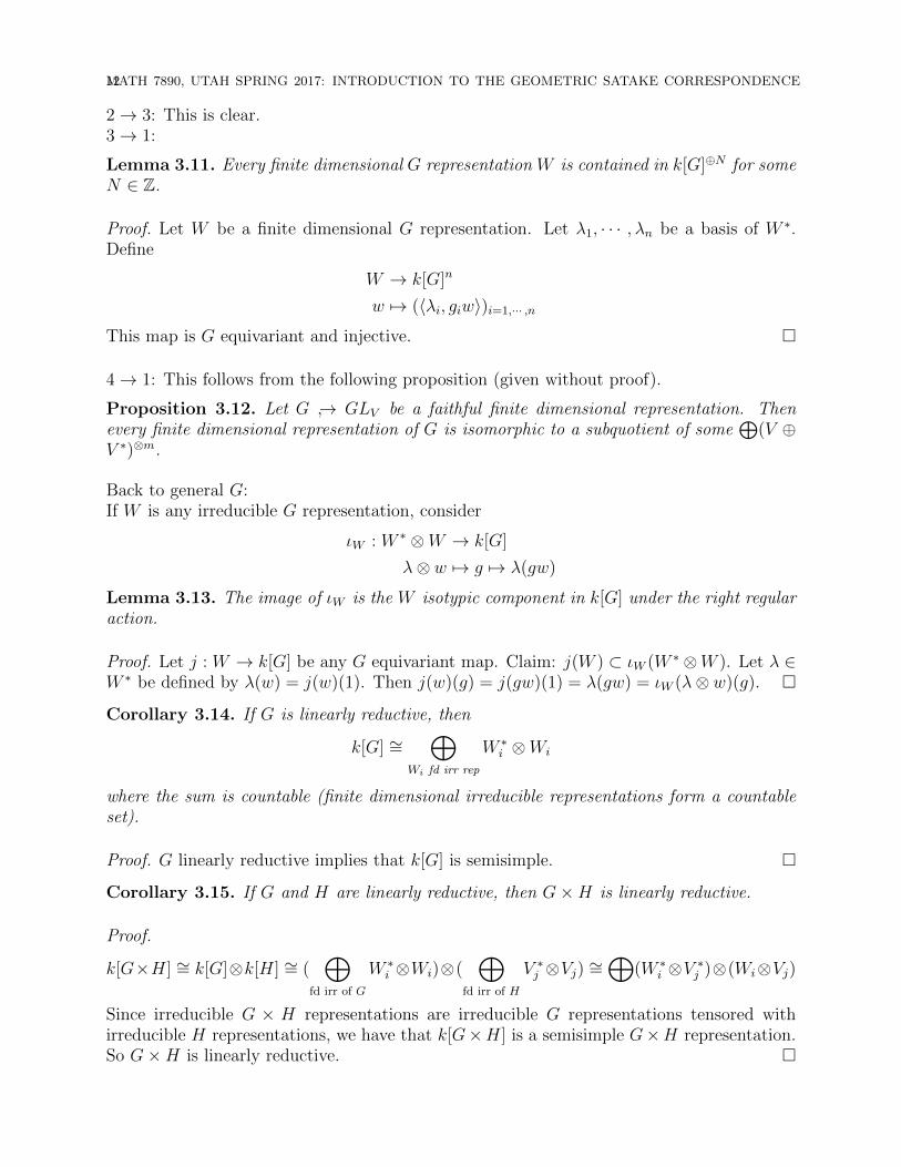
Definition 3.8. Let G be an algebraic group over k, V be a vector space over k (possiblyinfinite dimensional). A representation of G on V is a morphism of group valued functorsG→ GLV . Precisely, for all φ : R→ S we have the following commutative diagram
G(R) GLV (R)
GLV (S)G(S)
fR
fS
Note that if dimV <∞ then GLV is an algebraic group.
Example 3.9. Let us consider an infinite dimensional representation. Let k[G] be thecoordinate ring of G. Then k[G] is a G×G representation where
(g1, g2) · f(x) = f(g−11 xg2)
where g1, g2, x ∈ G and f ∈ k[G]. To frame this group action in our functorial definition ofa representation, we notice that
f ∈ Homk−alg(k[t], k[G]) = Hom(G,A1)
The groups of primary interest are the following:
Lemma 3.10. Let G be an algebraic group over k. The following are equivalent:
1. Finite dimensional representations of G are semisimple
2. Every representation of G is semisimple
3. k[G] is semisimple under either the right or left regular representation
4. There exists a faithful finite dimensional representation G → GLV so that for alln ≥ 1, V ⊗n is semisimple.
Such a group is called linearly reductive.
Some ideas of proof:1→ 2: Every representation is a filtered union of finite dimensional subrepresentations
12MATH 7890, UTAH SPRING 2017: INTRODUCTION TO THE GEOMETRIC SATAKE CORRESPONDENCE
2→ 3: This is clear.3→ 1:
Lemma 3.11. Every finite dimensional G representation W is contained in k[G]⊕N for someN ∈ Z.
Proof. Let W be a finite dimensional G representation. Let λ1, · · · , λn be a basis of W ∗.Define
W → k[G]n
w 7→ (〈λi, giw〉)i=1,··· ,n
This map is G equivariant and injective. �
4→ 1: This follows from the following proposition (given without proof).
Proposition 3.12. Let G ↪→ GLV be a faithful finite dimensional representation. Thenevery finite dimensional representation of G is isomorphic to a subquotient of some
⊕(V ⊕
V ∗)⊗m.
Back to general G:If W is any irreducible G representation, consider
ιW : W ∗ ⊗W → k[G]
λ⊗ w 7→ g 7→ λ(gw)
Lemma 3.13. The image of ιW is the W isotypic component in k[G] under the right regularaction.
Proof. Let j : W → k[G] be any G equivariant map. Claim: j(W ) ⊂ ιW (W ∗ ⊗W ). Let λ ∈W ∗ be defined by λ(w) = j(w)(1). Then j(w)(g) = j(gw)(1) = λ(gw) = ιW (λ⊗ w)(g). �
Corollary 3.14. If G is linearly reductive, then
k[G] ∼=⊕
Wi fd irr rep
W ∗i ⊗Wi
where the sum is countable (finite dimensional irreducible representations form a countableset).
Proof. G linearly reductive implies that k[G] is semisimple. �
Corollary 3.15. If G and H are linearly reductive, then G×H is linearly reductive.
Proof.
k[G×H] ∼= k[G]⊗k[H] ∼= (⊕
fd irr of G
W ∗i ⊗Wi)⊗(
⊕fd irr of H
V ∗j ⊗Vj) ∼=⊕
(W ∗i ⊗V ∗j )⊗(Wi⊗Vj)
Since irreducible G × H representations are irreducible G representations tensored withirreducible H representations, we have that k[G×H] is a semisimple G×H representation.So G×H is linearly reductive. �
MATH 7890, UTAH SPRING 2017: INTRODUCTION TO THE GEOMETRIC SATAKE CORRESPONDENCE13
3.3. Maximal Tori. We will begin this section with a short review and some supplementalmaterial from previous lectures:Fact: W is a finite group.
Proof. NG(T ) is closed, so NG(T ) is compact.
expT : t/lattice Λ→ T
is an isomorphism and W acts faithfully on Λ. So
W ↪→ AutZΛ
So W is compact and discrete, therefore finite. Example: If G = SU(n) then W = Sn. �
Definition 3.16. a k group scheme is a group object in the category of k-schemes. We sayit is algebraic if it is finite type over k.
Our groups of interest will be smooth affine algebraic groups (which we will further refer toas groups over k). Fact: If chark = 0, then an affine algebraic group is smooth.
Definition 3.17. A linearly reductive group G over k is a smooth affine algebraic groupsuch that all representations are semisimple.
Definition 3.18. A group T over k is a torus if
Tk ∼= Gnm
for some n ∈ Z, where Gm = GL1. We say T is split if T ∼= Gnm over k.
Example 3.19. Let k = R. R× is a split torus. S1 = S1(R) is a non split torus. C× = S(R)is a non split torus.
S : R-alg→ Grp
R 7→ Gm(C⊗R R)
Exercise: Show SC ∼= Gm ×Gm.
3.4. Representations of Tori.
Lemma 3.20. (1) Tori are linearly reductive.
(2) The simple representations of split torus Gnm are given by characters
χm1,··· ,mn : (t1, · · · , tn) 7→∏
tmii
Proof. Assume T is split, so T = Gnm. Then
k[T ] = k[X±11 , · · · , X±1
n ] =⊕Zn
kXm11 · · ·Xmn
n
which has summands that are stable under the right regular representation, and have char-acter χm1,··· ,mn . Since k[T ] is semisimple, T is linearly reductive. Since all simples appear ink[T ], χm1,··· ,mn exhaust characters of simple representations. �
Exercise: In characteristic 0, SLn is linearly reductive. In characteristic p > 0, SLn is notlinearly reductive.There is a different notion of a reductive group:
14MATH 7890, UTAH SPRING 2017: INTRODUCTION TO THE GEOMETRIC SATAKE CORRESPONDENCE
Definition 3.21. A group G over k is
(1) semisimple if the radical R(G) of Gk is trivial
(2) reductive if the unipotent radical Ru(Gk) is trivial
where R(G) is the maximal connected solvable smooth normal subgroup, and Ru(G) is themaximal connected unipotent smooth normal subgroup.
Example 3.22. (1)∗ · · · ∗0
. . ....
.... . . . . .
0 · · · 0 ∗
⊂ GLn is a solvable group
(2) 1 ∗ · · · ∗0
. . . . . ....
.... . . . . . ∗
0 · · · 0 1
= is a unipotent group
(3) (Exercise)
R(GLn) =
z 0 · · · 0
0. . . . . .
......
. . . . . . 00 · · · 0 z
= the center of GLn
(4) (Exercise)
Ru(GLn) = {1} ⇒ GLn is reductive not semisimple
(5) R(SLn) = {1} because (µn)◦ = {1} if char k does not divide n, and is not smooth ifchar k divides n.
Z(SLn) =
[z 00 z
]such that z ∈ µn
Fact: in characteristic 0, linearly reductive is equivalent to reductive.When studying representation theory we will focus on connected linearly reductive groupsover k = k with characteristic 0.
3.5. Structure Theory of Reductive Groups over k = k.
Definition 3.23. The Lie algebra of G is defined as
g = tangent space at 1 ∈ G= ker(G(k[ε])→ G(k))
MATH 7890, UTAH SPRING 2017: INTRODUCTION TO THE GEOMETRIC SATAKE CORRESPONDENCE15
where ε2 = 0.
Example 3.24. (1) If G = GLn then g = {1 + εA : A ∈Mn(k)}
(2) If G = SLn then g = {1 + εA : det(1 + εA) = 1} = {A ∈Mn(k) : trace(A) = 0}
(3) If G = Sp2n = {g ∈ GL2n : gtJg = J} where J is an alternating pairing, theng = {1 + εA ∈ GL2n(k[ε]) : (1 + εA)tJ(1 + εA) = J (equivalently AtJ + JA = 0)}
G acts on g by conjugation:
Ad : G→ Aut(g)
ad : g→ End(g)
ad(x)(y) := [x, y]
Now we will decompose g under AdT . Take G to be a connected reductive group with maxi-mal (split) torus T . We know T is linearly reductive so there is a semisimple decompositionof any representation of T .
V ∼=⊕
λ∈X•(T )
Vλ
For V = g,
g = g0 ⊕⊕
α∈Φ(G,T )
gα
where Φ(G, T ) = {0 6= λ ∈ X•(T ) : gλ 6= 0} denotes the set of roots of G with respect to T .
Example 3.25. Let GL3 ⊃ T = diagonal matrices
g = t⊕⊕α∈Φ
gα
where α ∈ {e1 − e2, e2 − e3, e1 − e3,−(e1 − e2), · · · }.X•(T ) = Ze1 ⊕ Ze2 ⊕ Ze3
where
ei
t1 t2t3
= ti
As in GL3, it is always the case that
g0 = {x ∈ g : Ad(t)(X) = X for all t ∈ T} = t
because the centralizer in G of T is T .
Key facts about maximal tori that generalize from the compact setting:Let G be a connected reductive algebraic group over k = k, with T a maximal torus.
(1) CG(T ) = T , W := N(T )/C(T )
(2) All maximal tori are conjugate (but not all g are conjugate to t ∈ T . Example:[1 10 1
]∈ SL2)
16MATH 7890, UTAH SPRING 2017: INTRODUCTION TO THE GEOMETRIC SATAKE CORRESPONDENCE
(3)⋃g∈G(k) gTg
−1 is Zariski dense in G.
Note: (2) is not true for k 6= k. Example: Consider G = SL2(R)
T1 =
[sin(θ) cos(θ)cos(θ) sin(θ)
]⊂ SL2(R) T2 =
[t 00 t−1
]⊂ SL2(R)
T1 and T2 are two non-conjugate maximal tori.
As before we have a map:
R(G) ↪→ R(T )W
Goal: We want to show that this is an isomorphism. First we need more structure theory(this will give us a definition of the Langlands dual group G∨). Immediate aim: classificationof connected reductive algebraic groups over k = k in terms of linear algebraic data.
Definition 3.26. A Borel subgroup in G is a maximal connected solvable subgroup.
Fact: All Borel subgroups in G are conjugate (if k = k).A choice of Borel T ⊂ B ⊂ G gives us a decomposition of roots Φ = Φ(G, T ) into ”positive”and ”negative” roots Φ+ = {α ∈ Φ : gα ⊂ b} and Φ− = −Φ+.
Example 3.27. ∗ ∗ ∗0 ∗ ∗0 0 ∗
⊂ GL3
g = t⊕⊕
Φ
gα Φ+ = {e1 − e2, e2 − e3, e1 − e3}
Fact: There is a set ∆ = {α1, · · · , αr} = ∆(G,B, T ) ⊂ Φ+(G,B, T ) of simple roots suchthat any positive root α ∈ Φ+ is uniquely expressible as α =
∑ciαi with ci ∈ Z≥0.
Our classification theorem for connected reductive groups over k = k rests on the followingrefinement of root systems.
Definition 3.28. A root datum is a 4-tuple (X,Φ, X∨,Φ∨) where
(1) X and X∨ are finite free Z-modules with perfect duality
〈, 〉 : X ×X∨ → Z
(2) Φ ⊂ X, Φ∨ ⊂ X∨ are finite subsets with fixed bijection α 7→ α∨ such that 〈α, α∨〉 = 2
(3) sα(Φ) = Φ and sα∨(Φ∨) = Φ∨
Where sα (sα∨) is a linear endomorphism of X (X∨) defined by
sα(x) = x− 〈x, α∨〉αsα∨(x∨) = x∨ − 〈α, x∨〉α∨
Structure Theorem:
Theorem. Connected reductive algebraic groups (up to isomorphism) over k = k are inbijection with root data (up to isomorphism).
MATH 7890, UTAH SPRING 2017: INTRODUCTION TO THE GEOMETRIC SATAKE CORRESPONDENCE17
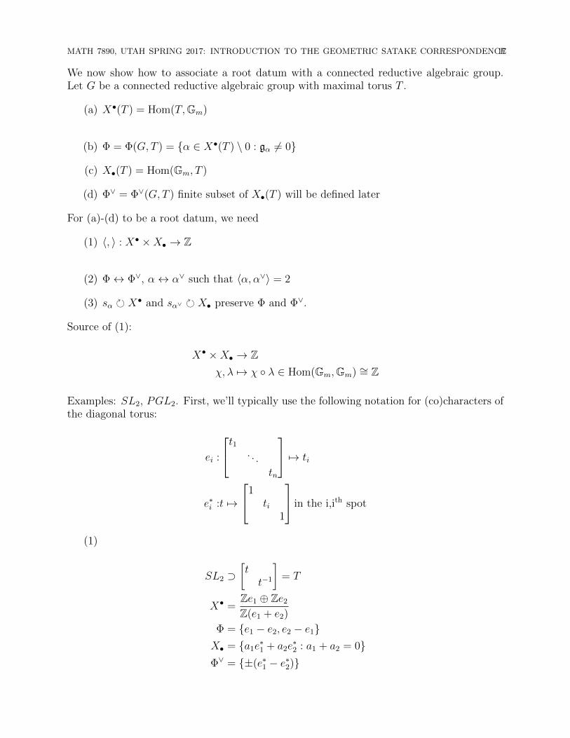
We now show how to associate a root datum with a connected reductive algebraic group.Let G be a connected reductive algebraic group with maximal torus T .
(a) X•(T ) = Hom(T,Gm)
(b) Φ = Φ(G, T ) = {α ∈ X•(T ) \ 0 : gα 6= 0}
(c) X•(T ) = Hom(Gm, T )
(d) Φ∨ = Φ∨(G, T ) finite subset of X•(T ) will be defined later
For (a)-(d) to be a root datum, we need
(1) 〈, 〉 : X• ×X• → Z
(2) Φ↔ Φ∨, α↔ α∨ such that 〈α, α∨〉 = 2
(3) sα � X• and sα∨ � X• preserve Φ and Φ∨.
Source of (1):
X• ×X• → Zχ, λ 7→ χ ◦ λ ∈ Hom(Gm,Gm) ∼= Z
Examples: SL2, PGL2. First, we’ll typically use the following notation for (co)characters ofthe diagonal torus:
ei :
t1 . . .tn
7→ ti
e∗i :t 7→
1ti
1
in the i,ith spot
(1)
SL2 ⊃[tt−1
]= T
X• =Ze1 ⊕ Ze2
Z(e1 + e2)
Φ = {e1 − e2, e2 − e1}X• = {a1e
∗1 + a2e
∗2 : a1 + a2 = 0}
Φ∨ = {±(e∗1 − e∗2)}
18MATH 7890, UTAH SPRING 2017: INTRODUCTION TO THE GEOMETRIC SATAKE CORRESPONDENCE
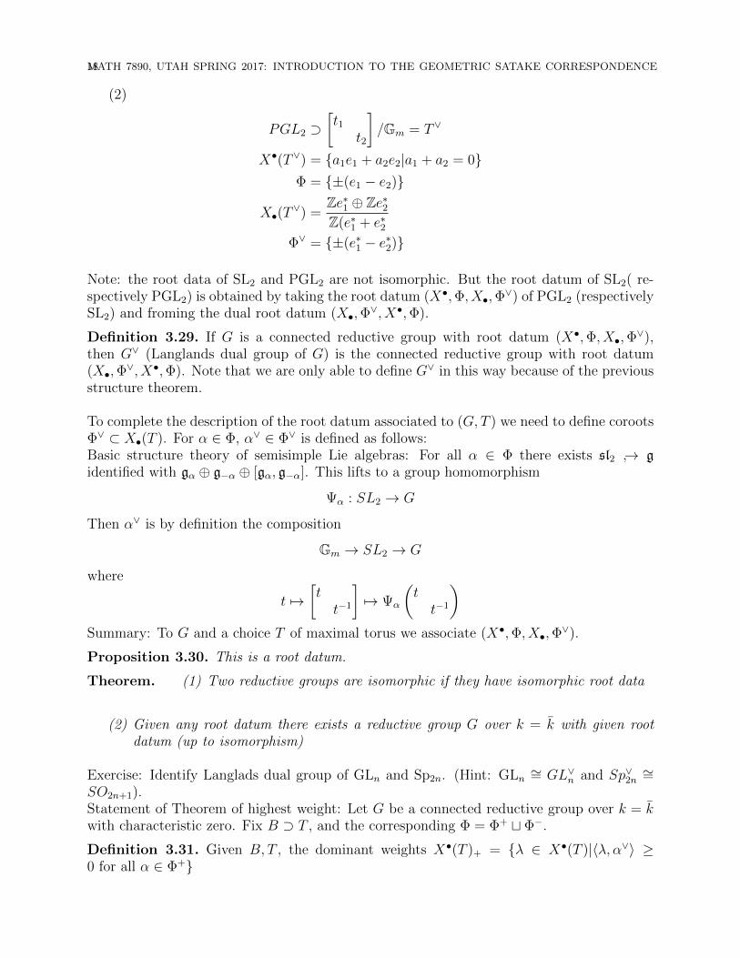
(2)
PGL2 ⊃[t1
t2
]/Gm = T∨
X•(T∨) = {a1e1 + a2e2|a1 + a2 = 0}Φ = {±(e1 − e2)}
X•(T∨) =
Ze∗1 ⊕ Ze∗2Z(e∗1 + e∗2
Φ∨ = {±(e∗1 − e∗2)}
Note: the root data of SL2 and PGL2 are not isomorphic. But the root datum of SL2( re-spectively PGL2) is obtained by taking the root datum (X•,Φ, X•,Φ
∨) of PGL2 (respectivelySL2) and froming the dual root datum (X•,Φ
∨, X•,Φ).
Definition 3.29. If G is a connected reductive group with root datum (X•,Φ, X•,Φ∨),
then G∨ (Langlands dual group of G) is the connected reductive group with root datum(X•,Φ
∨, X•,Φ). Note that we are only able to define G∨ in this way because of the previousstructure theorem.
To complete the description of the root datum associated to (G, T ) we need to define corootsΦ∨ ⊂ X•(T ). For α ∈ Φ, α∨ ∈ Φ∨ is defined as follows:Basic structure theory of semisimple Lie algebras: For all α ∈ Φ there exists sl2 ↪→ gidentified with gα ⊕ g−α ⊕ [gα, g−α]. This lifts to a group homomorphism
Ψα : SL2 → G
Then α∨ is by definition the composition
Gm → SL2 → G
where
t 7→[tt−1
]7→ Ψα
(tt−1
)Summary: To G and a choice T of maximal torus we associate (X•,Φ, X•,Φ
∨).
Proposition 3.30. This is a root datum.
Theorem. (1) Two reductive groups are isomorphic if they have isomorphic root data
(2) Given any root datum there exists a reductive group G over k = k with given rootdatum (up to isomorphism)
Exercise: Identify Langlads dual group of GLn and Sp2n. (Hint: GLn ∼= GL∨n and Sp∨2n∼=
SO2n+1).Statement of Theorem of highest weight: Let G be a connected reductive group over k = kwith characteristic zero. Fix B ⊃ T , and the corresponding Φ = Φ+ t Φ−.
Definition 3.31. Given B, T , the dominant weights X•(T )+ = {λ ∈ X•(T )|〈λ, α∨〉 ≥0 for all α ∈ Φ+}
MATH 7890, UTAH SPRING 2017: INTRODUCTION TO THE GEOMETRIC SATAKE CORRESPONDENCE19
Define a partial order on X•(T ) by λ ≥ µ if and only if λ−µ is a non negative integer linearcombination of α ∈ Φ+.
Example 3.32. SL2 and weights e1, and e1 − e2 ≡ 2e1 have no order relation
Definition 3.33. A representation V of G has highest weight λ (necessarily dominant) ifVλ 6= 0 and λ ≥ µ for all µ ∈ X•(T ) such that Vµ 6= 0.
Theorem. Every irreducible representation V of G has a highest weight λ (necessarily dom-inant) and the map
{ irr rep of G} → X•(T )+ is a bijection
V 7→ λ = hw(V )
Moreover, dimVλ = 1.
Corollary 3.34. The mapR(G)→ R(T )W
is an isomorphism
Proof. In every W orbit there is a unique B dominant weight. So a basis of right hand sideis given by
sλ =∑W
[wλ] for λ ∈ X•(T )+
We can complete the proof by using an upper triangular argument to show that {ch(V )}V ∈Irr
have a span containing all the sλ for λ ∈ X•(T )+. �
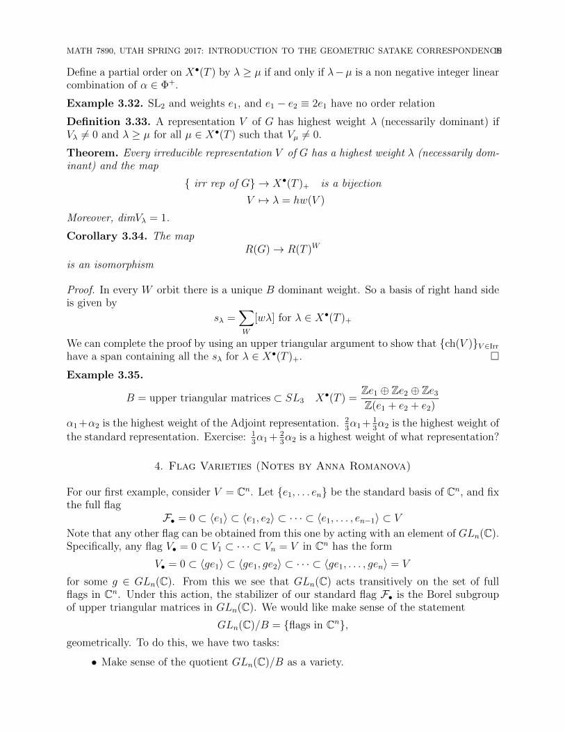
Example 3.35.
B = upper triangular matrices ⊂ SL3 X•(T ) =Ze1 ⊕ Ze2 ⊕ Ze3
Z(e1 + e2 + e2)
α1 +α2 is the highest weight of the Adjoint representation. 23α1 + 1
3α2 is the highest weight of
the standard representation. Exercise: 13α1 + 2
3α2 is a highest weight of what representation?
4. Flag Varieties (Notes by Anna Romanova)
For our first example, consider V = Cn. Let {e1, . . . en} be the standard basis of Cn, and fixthe full flag
F• = 0 ⊂ 〈e1〉 ⊂ 〈e1, e2〉 ⊂ · · · ⊂ 〈e1, . . . , en−1〉 ⊂ V
Note that any other flag can be obtained from this one by acting with an element of GLn(C).Specifically, any flag V• = 0 ⊂ V1 ⊂ · · · ⊂ Vn = V in Cn has the form
V• = 0 ⊂ 〈ge1〉 ⊂ 〈ge1, ge2〉 ⊂ · · · ⊂ 〈ge1, . . . , gen〉 = V
for some g ∈ GLn(C). From this we see that GLn(C) acts transitively on the set of fullflags in Cn. Under this action, the stabilizer of our standard flag F• is the Borel subgroupof upper triangular matrices in GLn(C). We would like make sense of the statement
GLn(C)/B = {flags in Cn},geometrically. To do this, we have two tasks:
• Make sense of the quotient GLn(C)/B as a variety.
20MATH 7890, UTAH SPRING 2017: INTRODUCTION TO THE GEOMETRIC SATAKE CORRESPONDENCE
• Make sense of the set {flags in Cn} as a variety.
We will examine these tasks from two perspectives. First, we will return to our categoricalperspective of algebraic groups as functors of points. Then, we will perform a more geometricconstruction.
5. The Functor of Points Perspective
Recall that we can apply the Yoneda embedding
Cop −→ Fun(C, Set)
to the category C of schemes over k and regard a variety or k-scheme X as its functor ofpoints
hX : k-alg −→ Set.
We need to determine how we can use this functor of points perspective to think aboutquotients of algebraic groups. We begin with a cautionary example. A first naive guess asto how to define quotients in this perspective would be to define the following functor:
GLn/B : k-alg −→ Set
R 7−→ GLn(R)/B(R)
To determine if this definition is what we’re looking for, we must ask ourselves if this functoris the functor of points of a scheme. The following exercise hints that this might not be thecase.
Exercise 5.1. Let n = 2, and R = Z[√−5] (notice that this is not a PID). Show that that
the mapGL2(Z[
√−5])/B(Z[
√−5]) −→ P1(Z[
√−5])
is not surjective.
This exercise illustrates that this functor does not give us the scheme we would expect(namely P1), so our definition of quotient needs some refinement (see Exercise 5.4 and The-orem 5.5 for a proof that this functor is not representable by a scheme). But first, we willdefine flag varieties in this categorical setting.
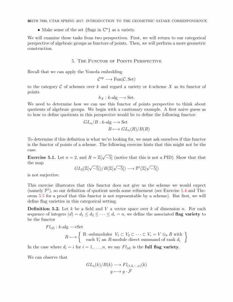
Definition 5.2. Let k be a field and V a vector space over k of dimension n. For eachsequence of integers (d) = d1 ≤ d2 ≤ · · · ≤ dr = n, we define the associated flag variety tobe the functor
Fl(d) : k-alg −→Set
R 7−→{
R -submodules V1 ⊂ V2 ⊂ · · · ⊂ Vr = V ⊗k R witheach Vi an R-module direct summand of rank di
}In the case where di = i for i = 1, . . . , n, we say Fl(d) is the full flag variety.
We can observe that
GLn(k)/B(k) −→ Fl(1,2,··· ,n)(k)
g 7−→ g · F
MATH 7890, UTAH SPRING 2017: INTRODUCTION TO THE GEOMETRIC SATAKE CORRESPONDENCE21
where F is a fixed flag with B = StabGLn(F), is an isomorphism. However, as our initialexample reveals, this doesn’t hold for general R; i.e.
GLn(R)/B(R) −→ Fl(R)
is not always surjective. The problem here from a functorial perspective is that the naivepresheaf quotient
(Aff/k)op −→ Set
R 7−→ GLn(R)/B(R)
“is not a sheaf.” We explain what this means precisely in the following pages.
We start by recalling the constructions of classical sheaf theory. For a topological space X,a presheaf on X is a functor
P : (OpenX)op −→ Set,
and a sheaf on X is a presheaf P that satisfies a glueing condition. We can define a similarnotion of sheaf on the category of topological spaces, Top. A presheaf on Top is a function
P : Topop −→ Set,
and a sheaf on Top is a presheaf P satisfying glueing conditions with respect to coveringfamilies of open immersions.
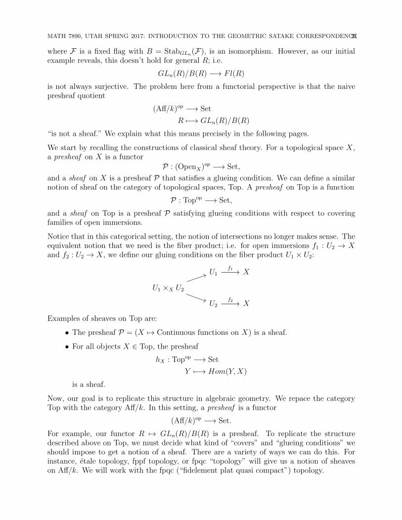
Notice that in this categorical setting, the notion of intersections no longer makes sense. Theequivalent notion that we need is the fiber product; i.e. for open immersions f1 : U2 → Xand f2 : U2 → X, we define our gluing conditions on the fiber product U1 × U2:
U1 X
U1 ×X U2
U2 X
f1
f2
Examples of sheaves on Top are:
• The presheaf P = (X 7→ Continuous functions on X) is a sheaf.
• For all objects X ∈ Top, the presheaf
hX : Topop −→ Set
Y 7−→ Hom(Y,X)
is a sheaf.
Now, our goal is to replicate this structure in algebraic geometry. We repace the categoryTop with the category Aff/k. In this setting, a presheaf is a functor
(Aff/k)op −→ Set.
For example, our functor R 7→ GLn(R)/B(R) is a presheaf. To replicate the structuredescribed above on Top, we must decide what kind of “covers” and “glueing conditions” weshould impose to get a notion of a sheaf. There are a variety of ways we can do this. Forinstance, etale topology, fppf topology, or fpqc “topology” will give us a notion of sheaveson Aff/k. We will work with the fpqc (“fidelement plat quasi compact”) topology.
22MATH 7890, UTAH SPRING 2017: INTRODUCTION TO THE GEOMETRIC SATAKE CORRESPONDENCE
In this setting, covers are jointly surjective familiies
d⊔i=1
SpecRi −→ SpecR
with each R→ Ri flat. This allows us to define a notion of a sheaf on the category Aff/k:
Definition 5.3. A sheaf for the fpqc topology is a presheaf
F : (Aff/k)op −→ Set
satisfying
(i) (locality) F(∏n
i=1 Ri) '∏n
i=1F(Ri), and
(ii) (gluing) For all faithfully flat ring homomorphisms R→ R′,
F(R)→ F(R′)p
⇒qF(R′ ⊗R R′)
is an equalizer diagram in the category Set; i.e. F(R) includes into F(R′) as {x ∈F(R′)|p(x) = q(x)}. Here, p is obtained from the ring homomorphism −⊗ 1 : R′ →R′ ⊗R R′ and q from 1⊗− : R′ −→ R′ ⊗R R′.
A follow-up exercise to the one at the beginning of this section is the following:
Exercise 5.4. Show that R 7→ GLn(R)/B(R) is not a sheaf for the fpqc topology.
We have the following theorem (Grothendieck’s theory of fpqc descent).
Theorem 5.5. For all objects X ∈ Aff/k, the representable functor hX is a sheaf in the fpqctopology.
This theorem suggests that the correct notion of quotients of algebraic groups in our categori-cal setting is that GLn/B should be the “sheafification1” of the presheaf R 7→ GLn(R)/B(R).And indeed, the results of the following section will indicate that this is the correct construc-tion. This ends our first perspective on the construction of the quotient. The philosophythat one should take away from this is that the correct approach is to “make the naiveconstruction in group theory, then make sure it’s a sheaf.”
6. The Geometric Perspective
Definition 6.1. Let G be an algebraic group over k. Let H ↪→ G be a Zariski closedsubgroup of G. Then a quotient X = G/H is a pair (X, π : G → X), where X is a schemeover k, satisfying
(i) π is faithfully flat,
(ii) π is right-H-invariant, and
1This is not technically well-defined. There is no sheafification functor for the fpqc topology. However,as long as the presheaves are “small enough,” sheafification will be possible, and the presheaves that we areinterested are “small enough.” For a precise statement of what it means for a presheaf to be “small enough”see William Charles Waterhouses article Basically Bounded Functors and Flat Sheaves.
MATH 7890, UTAH SPRING 2017: INTRODUCTION TO THE GEOMETRIC SATAKE CORRESPONDENCE23
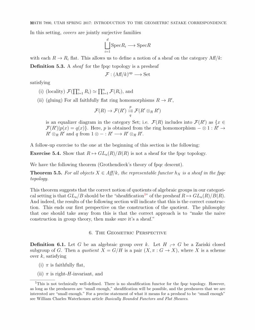
(iii) the map
G×H −→ G×X G(g, h) 7−→ (g, gh)
is an isomorphism; i.e. the non-empty fibers of G(R) → X(R) are just H(R)-orbitsfor all k-algebras R.
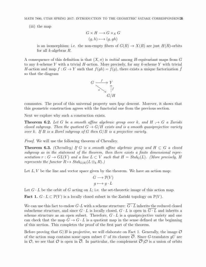
A consequence of this definition is that (X, π) is initial among H-equivariant maps from Gto any k-scheme Y with a trivial H-action. More precisely, for any k-scheme Y with trivialH-action and map f : G→ Y such that f(gh) = f(g), there exists a unique factorization fso that the diagram
G Y
G/H
π
f
f
commutes. The proof of this universal property uses fpqc descent. Morever, it shows thatthis geometric construction agrees with the functorial one from the previous section.
Next we explore why such a constuction exists.
Theorem 6.2. Let G be a smooth affine algebraic group over k, and H ↪→ G a Zariskiclosed subgroup. Then the quotient G→ G/H exists and is a smooth quasiprojective varietyover k. If B is a Borel subgroup of G then G/B is a projective variety.
Proof. We will use the following theorem of Chevalley.
Theorem 6.3. (Chevalley) If G is a smooth affine algebraic group and H ⊂ G a closedsubgroup as in the statement of the theorem, then there exists a finite dimensional repre-sentation r : G → GL(V ) and a line L ⊂ V such that H = StabG(L). (More precisely, Hrepresents the functor R 7→ StabG(R)(L⊗k R).)
Let L, V be the line and vector space given by the theorem. We have an action map:
G −→ P(V )
g 7−→ g · LLet G · L be the orbit of G acting on L; i.e. the set-theoretic image of this action map.
Fact 1. G · L ⊂ P(V ) is a locally closed subset in the Zariski topology on P(V ).
We can use this fact to endow G·L with a scheme structure: G · L inherits the reduced closedsubscheme structure, and since G · L is locally closed, G · L is open in G · L and inherits ascheme structure as an open subset. Therefore, G · L is a quasiprojective variety and onecan check that the map G → G · L is a quotient map in the sense defined at the beginningof this section. This completes the proof of the first part of the theorem.
Before proving that G/B is projective, we will elaborate on Fact 1. Generally, the image Oof the action map contains some open subset U of its closure O. Since G-translates gU arein O, we see that O is open in O. In particular, the complement O\O is a union of orbits
24MATH 7890, UTAH SPRING 2017: INTRODUCTION TO THE GEOMETRIC SATAKE CORRESPONDENCE
of strictly smaller dimension. We conclude that orbits of minimal dimension are necessarilyclosed.
Now we prove the second part of the theorem. Again, let L, V be the line and finite di-mensional vector space guaranteed by Chevalley’s theorem, so B = StabG(L) and G/B isconstructed as the image of the orbit map g 7→ g · L as before. Since B stabilizes L, B actson V/L, and since B is connected and solvable, it stabilizes a full flag V• = 0 ⊂ V1 ⊂ V2 ⊂· · · ⊂ VdimV/L = V/L in V/L. (This follows from the Lie-Kolchin Theorem.) We can lift thisflag to V , and we obtain a B-stable full flag V = 0 ⊂ L ⊂ V1 ⊂ V2 ⊂ · · · ⊂ V , where Viis the preimage of Vi under the quotient map. Since B = StabG(L), and V• is B-stable, wehave that B = StabG(V•). This gives us a new action of G on the full flag variety of GL(V ),
G→ Fl
g 7→ g · (0 ⊂ L ⊂ V1 ⊂ · · · ⊂ V )
Now, G/B is also the image of this action map. Furthermore, since B is a maximal connectedsolvable subgroup of G, G·(0 ⊂ L ⊂ V1 ⊂ · · · ⊂ V ) is an orbit of minimal dimension. Indeed,if F• is any flag and S = StabG(F•), then the connected component of the identity S◦ isconnected and solvable, so it is contained in a maximal connected solvable subgroup of G;i.e. a Borel subgroup B′. Since all Borel subgroups are conjugate, this implies
dimS◦ ≤ dimB, and thus dimG/B ≤ dimG/S◦ = dimG/S.
Therefore, G/B is an orbit of minimal dimension, so it is necessarily closed in Fl, which isa projective variety. This completes the proof of the theorem. �
Now we have two ways of thinking about quotients and we have found a family of projectivevarieties G/B. Our next step is to investigate the structure of these particular flag varietiesG/B.
7. The Bruhat Decomposition
We begin this section by recalling the structure of root subspaces of a reductive algebraicgroup. To a pair (G, T ), where G is a connected reductive group and T is a maximal torus, wecan associate a collection of roots Φ(G, T ) by decomposing G into simultaneous eigenspacesunder the Adjoint action of T , as described previously. Recall one of our key structuralresults of reductive algebraic groups: For α ∈ Φ(G, T ), there exists a homomorphism
ψα : SL2 −→ G,
obtained from the Lie algebra isomorphism sl2 −→ gα ⊕ g−α ⊕ [gα, g−α]. We define rootsubgroups Uα ⊂ G to be
Uα := ψα
((1 ∗0 1
))= exp(gα).
Let sα be the image of ψα
((0 1−1 0
))in the Weyl group W = W (G, T ) = NG(T )/T .
Fact 2. The set {sα}α∈∆(G,T,B) generates the Weyl group.
MATH 7890, UTAH SPRING 2017: INTRODUCTION TO THE GEOMETRIC SATAKE CORRESPONDENCE25
Now we turn our attention to the Bruhat decomposition. Let G be a connected reductivegroup over an algebraically closed field k = k. Let T ⊂ B ⊂ G be a choice of a torus and aBorel subgroup of G. Then B × B acts on G by (b1, b2) · g = b1gb
−12 . The orbits BgB are
locally closed subvarieties of G. (Note that these orbits are not always closed. For example,
if g ∈ B, then the orbit BgB = B ↪→ G is a closed subvariety. But if g =
(0 1−1 0
)∈ SL2,
then BgB is open in SL2.) For each w ∈ W , let w ∈ NG(T ) be a choice of lift. SetC(w) = BwB. Any choice of lift will give the same C(w), so this is well defined. Our goalof this section is to study the structure of these C(w).
Let N = Ru(B) be the unipotent radical of B. (For example, if B is the upper triangularBorel subgroup in GLn, N is the subgroup of upper triangular matrices with 1’s on thediagonal.) The following lemma reveals much about the structure of C(w).
Lemma 7.1. For w ∈ W , let R(w) = Φ+ ∩ (wΦ−) be the collection of positive roots thatare sent to negative roots under action by w−1. Let NR(w) be the subgroup of N generated by{Uα|α ∈ R(w)}. Then the multiplication map
NR(w)w ×B −→ C(w)
is an isomorphism of varieties. Moreover, the multiplication map∏α∈R(w)
Uα −→ NR(w)
is an isomorphism of varieties.2
Note that the space∏
α∈R(w) Uα is a product of affine spaces. The main result of this sectionis the following theorem.
Theorem 7.2. (Bruhat Decomposition)
G =⊔w∈W
C(w)
Exercise 7.3. Let G = SL2 and W =
{1,
(0 1−1 0
)}. Show directly that the theorem
holds in this case; i.e. that
SL2 = B tB(
0 1−1 0
)B,
where B is the Borel subgroup of upper triangular matrices.
The theorem immediately implies our main structural result about the projective varietiesG/B. Let Y (w) = C(w)/B. Such Y (w) are referred to as Bruhat cells. By lemma 3.1, Y (w)is an affine variety; i.e. Y (w) ' NR(w)w ×B/B ' A#R(w).
Corollary 7.4. The flag variety G/B is the disjoint union of Bruhat cells
G/B =⊔w∈W
Y (w).
2Note that this is not an isomorphism of groups.
26MATH 7890, UTAH SPRING 2017: INTRODUCTION TO THE GEOMETRIC SATAKE CORRESPONDENCE
This gives us an affine stratification of the flag variety.
Remark 7.5. The Bruhat cells Y (w) are locally closed subvarieties of G/B. Their closure,
X(w) := Y (w) is called the Schubert variety of w. These are complete, but may be singular.The singularities of Schubert varieties are of great representation-theoretic significance.
Example 7.6. For any G, there exists a unique element w0 ∈ W such that #R(w0) ismaximal. The number #R(w) is called the length of the element w ∈ W ,3 and defines alength function ` : W → Z by `(w) = #R(w). This unique element w0 is often referredto as the longest element of the Weyl group since its length is maximal. The associatedstratum Y (w0) is open and dense in G/B. This longest element w0 has the property thatw0(Φ−) = Φ+, so R(w0) = Φ+ ∩ (w0Φ−) = Φ+, and therefore NR(w0) = N .
Remark 7.7. There is a partial order on W characterized by v ≤ w if Y (v) ⊂ Y (w) = X(w).4
Now we give the idea of the proof of the theorem.
Proof. The proof relies on the following combinatorial result, which we will not prove.
Lemma 7.8. For all simple reflections sα, α ∈ ∆, and all w ∈ W ,
C(sα) · C(w) =
{C(sαw) if `(sαw) = `(w) + 1
C(sαw) ∪ C(w) if `(sαw) = `(w)− 1
Exercise 7.9. Check this for SL2.
Granted this lemma, we can deduce the decomposition G = tw∈WC(w) as follows:
(1) Let H = ∪w∈WC(w). We wish to show that H = G. The lemma implies thatC(sα) · H ⊂ H for all α ∈ ∆. But it can be shown that 〈C(sα)〉α∈∆ = G, soG ·H ⊂ H. We conclude that H = G.
(2) (Disjointness) Let w,w′ ∈ W and assume that C(w) ∩ C(w′) 6= ∅. Since both C(w)and C(w′) are B × B-orbits, this can only happen if C(w) = C(w′). In particular,`(w) = `(w′). We use induction in `(w) to show that w = w′. If `(w) = `(w′) = 0,then w = 1 = w′ and we are done, so we assume `(w) > 0. Then there exists sα forα ∈ ∆ such that `(sαw) = `(w)− 1. By the lemma,
C(sαw) ⊂ C(sα) · C(w) = C(sα) · C(w′) ⊂ C(sαw′) ∪ C(w′).
This implies that C(sαw) = C(sαw′) or C(sαw) = C(w′). Since dimC(w′) =
dimC(sαw) + 1, the latter is impossible. Therefore, we can imply the inductionhypothesis to C(sαw) = C(sαw
′), and we are done.
�
3The number #R(w) can also be described combinatorially by expressing an element w ∈W as a productof simple reflections. The minimal number of simple reflections needed to express w is a well-defined invariantand it agrees with the cardinality of R(w). This explains the nomenclature “length.” For more informationon the combinatorics of Coxeter groups, see James E. Humphreys Reflection Groups and Coxeter Groups.
4This partial order can also be realized combinatorially in terms of the length.
MATH 7890, UTAH SPRING 2017: INTRODUCTION TO THE GEOMETRIC SATAKE CORRESPONDENCE27
8. Borel-Weil Theorem and Theorem of highest weight (notes by AllecharSerrano Lopez)
Our main goal is to construct a highest weight λ irreducible representation of G for allλ ∈ X•(T )+ and to show that these are all the irreducible representations of G. Our approachis via the Borel-Weil theorem. Recall that, given a representation V of a connected reductivegroup G (containing a fixed Borel subgroup B and a fixed maximal torus T ≤ B) and achoice of a highest weight vector v ∈ V , we get a G-equivariant map
G/B → P(V )
v 7→ (gv).
The idea of the Borel-Weil theorem is to run this argument in reverse: we construct G-equivariant line bundles on G/B and study the associated maps (see above) to projectivespaces. We begin with some preliminaries on highest weights.
Lemma 8.1. If V is a highest weight λ representation, then λ is dominant.
Proof. Recall that ch(V ) is W−invariant. So if Vλ 6= 0, then Vsα(λ) 6= 0 for all sα(λ) ∈ W .By assumption, λ > sα(λ), i.e., 〈λ, α∨〉α ∈ Z>0Φ+, so 〈λ, α∨〉 > 0 for all α ∈ Φ+. �
Definition 8.2. Let V be a representation of G. Say that v ∈ V is a highest weight vectorof highest weight λ if Nv = v (or nv = 0, where n = Lie(N)) and T acts on V by λ.
Example 8.3. Consider G = SL2 and V = Sym3C2 ⊕ Sym4C2, where 〈e1, e2〉 and 〈f1, f2〉generate C in the first and second summands, respectively. We have that e3
1 ∈ Sym3C2 and
f 41 ∈ Sym4C2. Then e3
1 and f 41 are the highest weight vectors of weights
(t 00 t−1
)7→ t3, t4,
respectively; but, V is not a highest weight representation in the sense just defined.
Lemma 8.4. If V is a highest weight representation of weight λ, then any v ∈ Vλ r 0 is ahighest weight vector of weight λ.
Proof. We need to show that nv = 0. More generally, if α ∈ Φ, and if Xα ∈ gα, thenXα · Vλ ⊂ Vλ+α ∪ 0: for all t ∈ T
t ·Xαv = Ad(t)Xα · tv = α(t)Xαλ(t)v = (α + λ)(t)Xαv
In particular, in our highest weight λ representation V , Vα+λ = 0 for all α ∈ Φ+, so nv = 0,i.e., v ∈ Vλ is a highest weight vector. �
Lemma 8.5. If V is any non-zero G−representation, the V contains a highest weight vectorwith dominant weight.
Proof. Let λ be any weight in V that is maximal for the partial order ≤, and let v be anynon-zero element of the weight space Vλ. Since λ is maximal, the argument of the previouslemma shows v is a highest weight vector. The argument of Lemma 8.1 (i.e., W -invarianceof the character) then shows λ is dominant. �
Combined with semi-simplicity of G-representations, this lemma implies:
Corollary 8.6. If dimV N 6 1, then V is irreducible.
28MATH 7890, UTAH SPRING 2017: INTRODUCTION TO THE GEOMETRIC SATAKE CORRESPONDENCE
That concludes the preliminaries. Now we turn to the construction of highest weight rep-resentations; the Borel-Weil theorem finds these in the cohomology of G-equivariant linebundles on the flag variety G/B, so we start by reviewing a few facts about linear systems.
Recall that for any variety X over k, we have the following bijection:
{maps Xf−→ P(V )} ←→
{base-point free linear system (L, V, i : V ∗ → Γ(X,L))
}/ ∼=
f 7−→(f ∗(O(1)), i : V ∗ → Γ(X,L) with the property that for all
x ∈ X there exists α ∈ V ∗ such that i(α)|x 6= 0
)Recall that P(V ) has a tautological line bundle O(−1) whose fiber over a line l is just the linel; the dual line bundle O(1) has fiber l∗ = Homk(l, k) over l, and Γ(P(V ),O(1)) is canonicallyisomorphic to V ∗, via the map sending α ∈ V ∗ to the section l 7→ α|l.
We want to upgrade this correspondence to a G−equivariant version:
Corollary 8.7. If X is a space with G−action and V is a G−representation, then there isa bijection
{G− equivariant maps X → P(V )} ↔{G− equivariant base point free linear systems (L, V, ι) on X}/ ∼=
Here is the precise definition of a G-equivariant linear system:
Definition 8.8. A G−equivariant linear system on X is (L, V, i : V ∗ → Γ(X,L)) such that
1) L is a G−equivariant line bundle on X. This means that L is a line bundle on Xequipped with a G−action compatible with the action on X under the projectionL → X, and for all x ∈ X and all g ∈ G, the map g : Lx → Lg·x is linear.
2) V is a G−representation.
3) i is a map of G−representations (see below).
In part (3) of the above definition, we define the action of G on Γ(X,L) as follows. For asection s : X → L, and g ∈ G, define g · s ∈ Γ(X,L) by setting (g · s)(x) = gs(g−1x) .
Lemma 8.9. The correspondence
{G−equivariant line
bundles on G/B
}←→
{1−dimensional
B−representations
}L 7−→ LB
induces a bijection
{G− equivariant linebundles on G/B} / ∼= ∼−→ Hom(B,Gm)
Proof. We will construct the inverse map. Given χ : B → Gm, we form the associated linebundle
MATH 7890, UTAH SPRING 2017: INTRODUCTION TO THE GEOMETRIC SATAKE CORRESPONDENCE29
G×B A1 = {(g, x) ∈ G× A1}/(gb, x) ∼ (g, χ(b)x)→ G/B
where the equivalence relation is defined for all g ∈ G, x ∈ A1, b ∈ B. Analytically, this isclearly a line bundle. In the Zariski topology, we use the fact that the map G→ G/B Zariski-locally has sections (this follows from the description of the big Bruhat cell C(w0) = N×B).
�
Lemma 8.10. Hom(B,Gm) = Hom(T,Gm) = X•(T ).
Proof. Any homomorphism B → Gm is trivial on N (we have shown this before; it reducesto showing that Hom(Ga,Gm) = 0), hence factors as a homomorphism
T∼−→ B/N → Gm.
�
Definition 8.11. For λ ∈ X•(T ), define L(λ) = G×B k(−λ) to be the line bundle on G/Bassociated to −λ.
We can now state the main theorem:
Theorem 8.12 (Borel-Weil). Let G be a connected, reductive group with B ≤ G a Borelsubgroup and T ≤ B a maximal torus. Then:
1) If λ ∈ X•(T )+, then V (λ) := H0(G/B,L(λ))∗ is an irreducible G-representation withhighest weight λ.
2) The V (λ) constructed in this way exhaust all the irreducible representations of G upto isomorphism.
3) If λ ∈ X•(T )\X•(T )+, then H0(G/B,L(λ)) = 0.
4) dimV (λ)λ = 1.
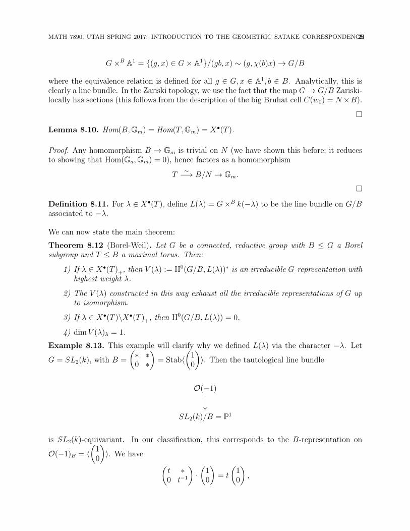
Example 8.13. This example will clarify why we defined L(λ) via the character −λ. Let
G = SL2(k), with B =
(∗ ∗0 ∗
)= Stab〈
(10
)〉. Then the tautological line bundle
O(−1)
SL2(k)/B = P1
is SL2(k)-equivariant. In our classification, this corresponds to the B-representation on
O(−1)B = 〈(
10
)〉. We have (
t ∗0 t−1
)·(
10
)= t
(10
),
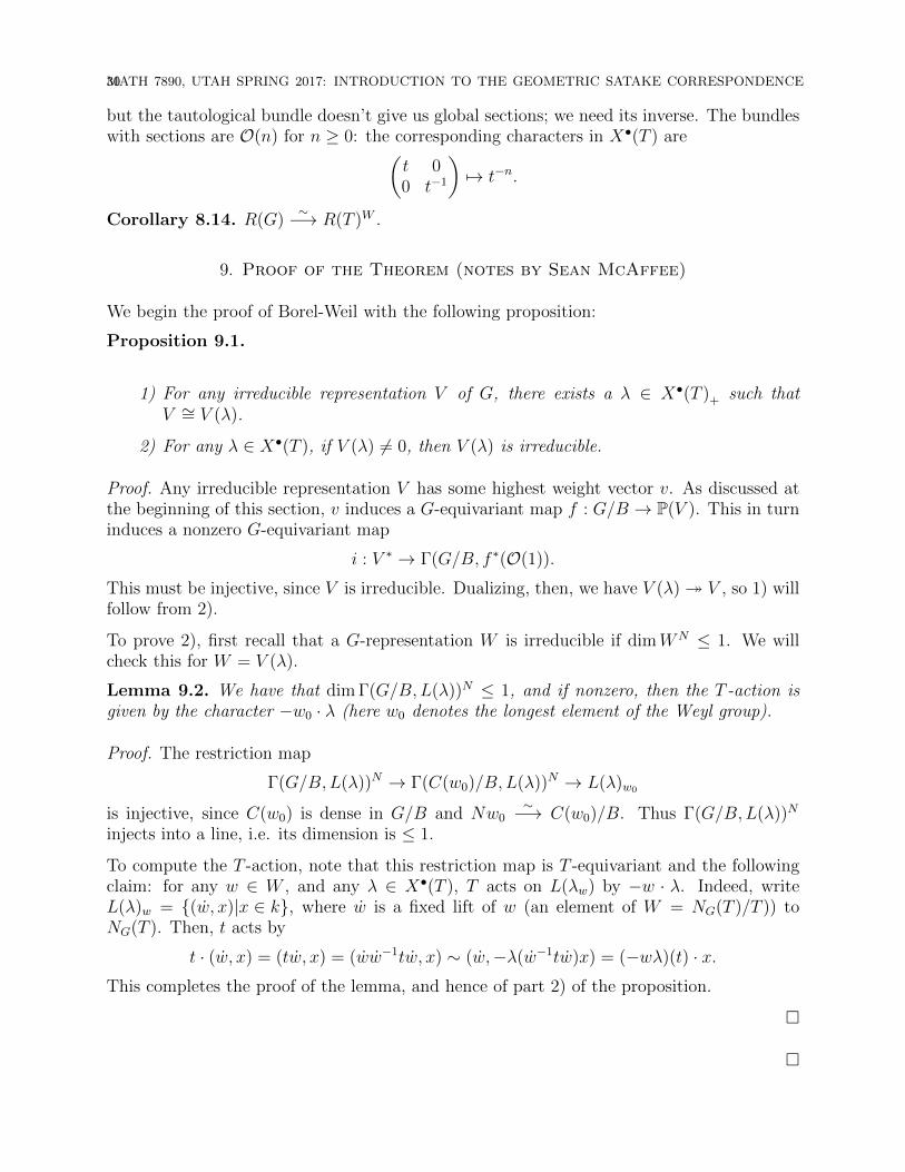
30MATH 7890, UTAH SPRING 2017: INTRODUCTION TO THE GEOMETRIC SATAKE CORRESPONDENCE
but the tautological bundle doesn’t give us global sections; we need its inverse. The bundleswith sections are O(n) for n ≥ 0: the corresponding characters in X•(T ) are(
t 00 t−1
)7→ t−n.
Corollary 8.14. R(G)∼−→ R(T )W .
9. Proof of the Theorem (notes by Sean McAffee)
We begin the proof of Borel-Weil with the following proposition:
Proposition 9.1.
1) For any irreducible representation V of G, there exists a λ ∈ X•(T )+ such thatV ∼= V (λ).
2) For any λ ∈ X•(T ), if V (λ) 6= 0, then V (λ) is irreducible.
Proof. Any irreducible representation V has some highest weight vector v. As discussed atthe beginning of this section, v induces a G-equivariant map f : G/B → P(V ). This in turninduces a nonzero G-equivariant map
i : V ∗ → Γ(G/B, f ∗(O(1)).
This must be injective, since V is irreducible. Dualizing, then, we have V (λ)� V , so 1) willfollow from 2).
To prove 2), first recall that a G-representation W is irreducible if dimWN ≤ 1. We willcheck this for W = V (λ).
Lemma 9.2. We have that dim Γ(G/B,L(λ))N ≤ 1, and if nonzero, then the T -action isgiven by the character −w0 · λ (here w0 denotes the longest element of the Weyl group).
Proof. The restriction map
Γ(G/B,L(λ))N → Γ(C(w0)/B, L(λ))N → L(λ)w0
is injective, since C(w0) is dense in G/B and Nw0∼−→ C(w0)/B. Thus Γ(G/B,L(λ))N
injects into a line, i.e. its dimension is ≤ 1.
To compute the T -action, note that this restriction map is T -equivariant and the followingclaim: for any w ∈ W , and any λ ∈ X•(T ), T acts on L(λw) by −w · λ. Indeed, writeL(λ)w = {(w, x)|x ∈ k}, where w is a fixed lift of w (an element of W = NG(T )/T )) toNG(T ). Then, t acts by
t · (w, x) = (tw, x) = (ww−1tw, x) ∼ (w,−λ(w−1tw)x) = (−wλ)(t) · x.This completes the proof of the lemma, and hence of part 2) of the proposition.
�
�
MATH 7890, UTAH SPRING 2017: INTRODUCTION TO THE GEOMETRIC SATAKE CORRESPONDENCE31
To complete the proof of Borel-Weil, we need to show that Γ(G/B,L(λ)) is nonzero if andonly if λ is dominant. First, we show that Γ 6= 0 implies λ is dominant. We do thisby analyzing the possible weights of Γ. We have seen that restriction to C(wo) gives aT -equivariant injection
Γ(G/B,L(λ)) ↪→ Γ(Y (w0), L(λ)).
Let λ∗ denote −w0 · λ, and let n denote Lie(N). We have that T acts on n via Ad, hence Tacts on the dual n∗.
Lemma 9.3.
Γ(Y (w0), L(λ)) ∼=T k(λ∗)⊗ Sym•(n∗).
(Here ∼=T denotes isomorphism as T -representations). In particular, this is a highest weightrepresentation with highest weight λ∗.
Proof. Recall the isomorphism
N∼−→ Y (w0)
n 7→ nw0.
Under this map, the left T -action on Y (w0) intertwines Ad(T ) on N :
tnw0 = tnt−1tw0 = tnt−1w0t′ ∼ Ad(t)nw0.
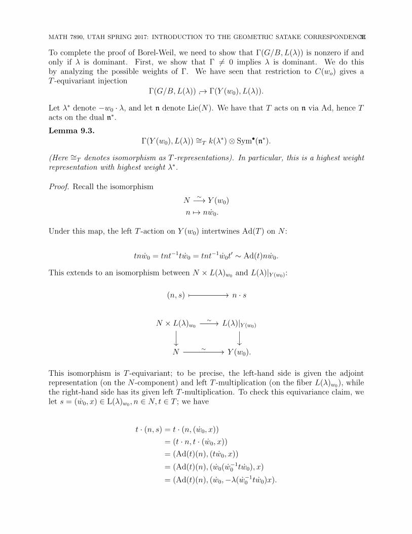
This extends to an isomorphism between N × L(λ)w0 and L(λ)|Y (w0):
(n, s) n · s
N × L(λ)w0 L(λ)|Y (w0)
N Y (w0).
∼
∼
This isomorphism is T -equivariant; to be precise, the left-hand side is given the adjointrepresentation (on the N -component) and left T -multiplication (on the fiber L(λ)w0), whilethe right-hand side has its given left T -multiplication. To check this equivariance claim, welet s = (w0, x) ∈ L(λ)w0 , n ∈ N, t ∈ T ; we have
t · (n, s) = t · (n, (w0, x))
= (t · n, t · (w0, x))
= (Ad(t)(n), (tw0, x))
= (Ad(t)(n), (w0(w−10 tw0), x)
= (Ad(t)(n), (w0,−λ(w−10 tw0)x).
32MATH 7890, UTAH SPRING 2017: INTRODUCTION TO THE GEOMETRIC SATAKE CORRESPONDENCE
Via this T -equivariant trivialization of L(λ)|Y (w0), we can compute
Γ(Y (w0), L(λ)) ∼=T Γ(N,N × L(λ)w0) ∼=T O(N)⊗ k(λ∗) ∼= Sym•(n∗)⊗ k(λ∗).
This completes the proof of the lemma, and the proposition follows.
�
The main step in the proof of Borel-Weil is to show that for any λ ∈ X•(T )+ we have
H0(G/B,L(λ)) 6= 0. To show this, our strategy will be to construct a highest weight vectorof weight λ∗. We will do this in two steps:
Step 1: Construct the highest weight vector over the “big cell” Y (w0).
Step 2: Show that this section extends to all of G/B.
First, we remark that a section s on the line bundle
G×B k(−λ)
G/B
can be viewed as a map gB 7→ (g, f(g)) for some function f : G → k. Since gB = gbB, wemust have (g, f(g)) = (gb, f(gb)) for all g ∈ G, b ∈ B. Furthermore, the equivalence relationon G×B k(−λ) requires
(gb, f(gh)) ∼ (g,−λ(b)f(gb)).
Thus, we can think of sections as being determined by a function f : G→ k such that
f(gb) = λ(b)f(g),∀g ∈ G, b ∈ B.Under this correspondence, the G-action on a section s translates into the left regular actionon a function f with the above properties.
We have that N × T × N and C(w0) = Nw0B are isomorphic as varieties under the map(n1, t, n2) 7→ n1w0tn2; we define a function f on C(w0) by
f(n1w0tn2) := λ(t).
We claim that f is a highest weight vector of weight λ∗ := −w0λ. Indeed, N · f = f since fis left N -invariant by the left regular action, and we have
(t1 · f)(n1w0tn2) = f(t−11 n1w0tn2)
= f((t−11 n1t1)t−1
1 w0tn2)
= f(t−11 w0tn2)
= f(w0(w−10 t−1
1 w0) · tn2)
= λ(w−10 t−1
1 w0t)
= (−w0λ)(t1)λ(t).
MATH 7890, UTAH SPRING 2017: INTRODUCTION TO THE GEOMETRIC SATAKE CORRESPONDENCE33
This completes Step 1. Now, for the second (and final) step, we need to extend the sectiondefined above to all of G/B. To do this, we first extend to a section on an open subsetU ⊂ G/B such that the complement of U has codimension ≥ 2. Then, we use the analyticcontinuation principle: for a line bundle L on an irreducible normal variety X, the restrictionmap Γ(X,L)→ Γ(U,L) is surjective when the codimension of X − U is ≥ 2.
Given f as above, we extend f from C(w0) = Nw0B to
C(w0) ∪⋃α∈∆
sαNw0B.
Note that each sαNw0B is open, but contains C(sαw0), and in this way the union underconsideration contains all Bruhat cells of codimension one.
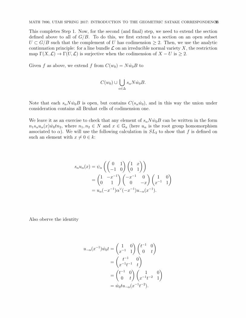
We leave it as an exercise to check that any element of sαNw0B can be written in the formn1sαuα(x)w0tn2, where n1, n2 ∈ N and x ∈ Ga (here uα is the root group homomorphismassociated to α). We will use the following calculation in SL2 to show that f is defined onsuch an element with x 6= 0 ∈ k:
sαuα(x) = ψα
((0 1−1 0
)(1 x0 1
))=
(1 −x−1
0 1
)(−x−1 0
0 −x
)(1 0x−1 1
)= uα(−x−1)α∨(−x−1)u−α(x−1).
Also oberve the identity
u−α(x−1)w0t =
(1 0x−1 1
)(t−1 00 t
)=
(t−1 0
x−1t−1 t
)=
(t−1 00 t
)(1 0
x−1t−2 1
)= w0tu−α(x−1t−2).
34MATH 7890, UTAH SPRING 2017: INTRODUCTION TO THE GEOMETRIC SATAKE CORRESPONDENCE
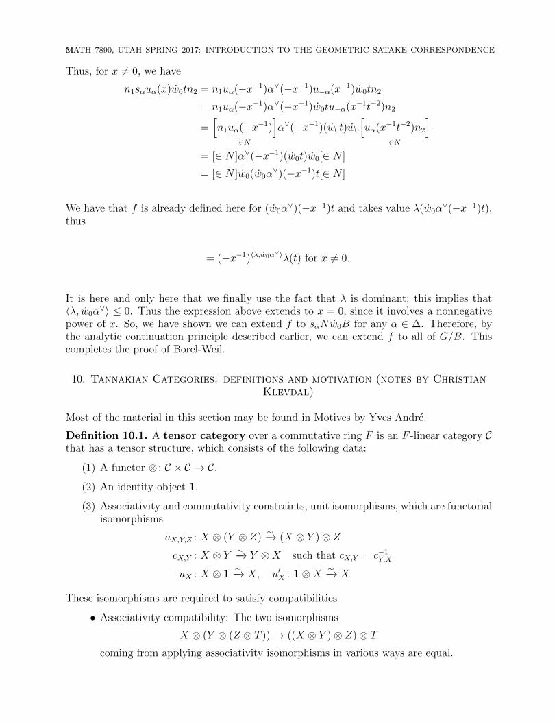
Thus, for x 6= 0, we have
n1sαuα(x)w0tn2 = n1uα(−x−1)α∨(−x−1)u−α(x−1)w0tn2
= n1uα(−x−1)α∨(−x−1)w0tu−α(x−1t−2)n2
=[n1uα(−x−1)
]∈N
α∨(−x−1)(w0t)w0
[uα(x−1t−2)n2
]∈N
.
= [∈ N ]α∨(−x−1)(w0t)w0[∈ N ]
= [∈ N ]w0(w0α∨)(−x−1)t[∈ N ]
We have that f is already defined here for (w0α∨)(−x−1)t and takes value λ(w0α
∨(−x−1)t),thus
= (−x−1)〈λ,w0α∨〉λ(t) for x 6= 0.
It is here and only here that we finally use the fact that λ is dominant; this implies that〈λ, w0α
∨〉 ≤ 0. Thus the expression above extends to x = 0, since it involves a nonnegativepower of x. So, we have shown we can extend f to sαNw0B for any α ∈ ∆. Therefore, bythe analytic continuation principle described earlier, we can extend f to all of G/B. Thiscompletes the proof of Borel-Weil.
10. Tannakian Categories: definitions and motivation (notes by ChristianKlevdal)
Most of the material in this section may be found in Motives by Yves Andre.
Definition 10.1. A tensor category over a commutative ring F is an F -linear category Cthat has a tensor structure, which consists of the following data:
(1) A functor ⊗ : C × C → C.
(2) An identity object 1.
(3) Associativity and commutativity constraints, unit isomorphisms, which are functorialisomorphisms
aX,Y,Z : X ⊗ (Y ⊗ Z)∼−→ (X ⊗ Y )⊗ Z
cX,Y : X ⊗ Y ∼−→ Y ⊗X such that cX,Y = c−1Y,X
uX : X ⊗ 1∼−→ X, u′X : 1⊗X ∼−→ X
These isomorphisms are required to satisfy compatibilities
• Associativity compatibility: The two isomorphisms
X ⊗ (Y ⊗ (Z ⊗ T ))→ ((X ⊗ Y )⊗ Z)⊗ Tcoming from applying associativity isomorphisms in various ways are equal.
MATH 7890, UTAH SPRING 2017: INTRODUCTION TO THE GEOMETRIC SATAKE CORRESPONDENCE35
• Compatibility of commutativity and associativity: The two isomorphisms
X ⊗ (Y ⊗ Z)→ (Z ⊗X)⊗ Ycoming from applying associativity and commutativity isomorphisms in various waysare equal.
• Compatibility of associativity and unit: The two isomorphisms
X ⊗ (1⊗ Y )→ X ⊗ Ycoming from applying associativity and unit isomorphisms in various ways are equal.
Further, the tensor category (C,⊗) is said to be rigid if:
(4) There exists an autoduality ∨ : C → Cop such that for each object X, the functor-⊗X∨ is left adjoint to -⊗X and X∨ ⊗ - is right adjoint to X ⊗ -.
Note that if (C,⊗) is a rigid tensor category then the unit and counit of adjunction give mapsε : X ⊗X∨ → 1 and η : 1 → X∨ ⊗X called evaluation and coevaluation respectively. Onecan now define a trace map from End(X) to the commutative F -algebra End(1) sendingf ∈ End(X) to the composition
1f−→ X∨ ⊗X
cX∨,X−−−→ X ⊗X∨ ε−→ 1
The first map is induced by f using adjunction Hom(X,X) ∼= Hom(1, X∨ ⊗X). We definethe rank of X to be the the trace of the identity, that is ε ◦ cX∨,X ◦ η ∈ End(1).
Example 10.2. If F is a field and G a group then the category of RepF (G) is a rigidtensor category, where ⊗ is the usual tensor product,1 is the trivial representation and V ∨
is the dual. Note End(1) = F and the rank of an object V is just the dimension of therepresentation.
Definition 10.3. A tensor functor between tensor categories (C,⊗C), (T ,⊗T ) over F isan F linear functor ω : C → T with functorial isomorphisms
oX,Y : ω(X ⊗C Y )∼−→ ω(X)⊗T ω(Y ) o1 : ω(1C)
∼−→ 1T
that are compatible with constraints a, c, u, u′.
We can finally define what a (neutral) Tannakian category is.
Definition 10.4. Suppose (C,⊗) is a rigid abelian tensor category, i.e. C is abelian and ⊗is bi-additive. Let K = End(1). A fiber functor for C is an exact, faithful tensor functor
ω : C → VectL
to the category of finite dimensional L-vector spaces, where L ⊃ K. If such a fiber functorexists, we say that C is Tannakian. If L = K then we say that C is neutral Tannakian.
10.1. Homological Motives. The interest in Tannakian categories in algebraic geometrycomes from motives, which we quickly review here. Much of the following is imprecise.For reference, one should consult the book Motives by Yves Andre or the article ClassicalMotives by A.J. Scholl. For any field k, we can define the category of pure homologicalmotives over k with coefficients in a field F . In order to define motives, we first need torecall facts about algebraic cycles. Given a variety X over k, and a field F denote Zr
F (X) to
36MATH 7890, UTAH SPRING 2017: INTRODUCTION TO THE GEOMETRIC SATAKE CORRESPONDENCE
be the free F -module generated by irreducible subvarieties of codimension r. An element ofZrF (X) is called an algebraic cycle. A Weil cohomology theory is a functor H∗ from smooth
projective varieties over k to finite dimensional graded commutative F -algebras with a cycleclass map Zr
F (X) → H2r(X) satisfying Poincare duality and the Kunneth formula (alongwith certain compatability and non degeneracy conditions). The typical examples are `-adic cohomology, algebraic de Rham cohomology and if k ⊂ C singular cohomology. Ifwe fix a Weil cohomology theory, one can define an equivalence relation called homologicalequivalence on Zr
F (X) by Z ∼H W if they have the same image under the cycle classmap. Define Ar(X) = Zr
F (X)/ ∼H . Given a map of varieties (which will mean smoothprojective from now on) f : X → Y there are pull back maps f ∗ : Ar(Y ) → Ar(X) andpushforward maps f∗ : A
r(X) → Ar+dim(Y )−dim(X)(Y ). There is also a product structureAr(X) ⊗ As(X) → Ar+s(X), denoted by Z ⊗W 7→ Z ·W . For connected varieties X, Ywe define the correspondences of degree r to be Corrr(X, Y ) = Adim(X)+r(X × Y ). Wecan define a composition law Corrr(X, Y ) × Corrs(Y, Z) → Corrr+s(X,Z) given on cyclesZ ∈ Corrr(X, Y ),W ∈ Corrs(Y, Z) by
Z ◦W = (pXZ)∗(p∗XYZ · p∗Y ZW )
where the p maps are the various projections from X × Y × Z. We may finally define thecategory of pure homological motivesMk over F . The objects are triples (X, p, r) where Xis a (smooth projective) variety over k, p ∈ Corr0(X,X) is an idempotent correspondenceand r is an integer. One should think of a motive as a ‘chunk of cohomology’, correspondingto the image pH∗(X)(r). For example, if X is smooth and projective and x ∈ X one cancheck that {x}×X induces projection H∗(X)→ H0(X) for any Weil cohomology theory. Inthis case we say that the H0 projector is algebraic. It is conjectured that all (“K unneth”)projectors H∗(X)→ H i(X) are algebraic.
We still need to define maps between motives. Given another motive (Y, q, s),
HomMk((X, p, r), (Y, q, s)) = pCorrs−r(X, Y )q
Composition is given by composition of correspondences. There is a functor
h : Varopk →Mk, X 7→ h(X) = (X,∆X , 0)
from the category of smooth projective varieties over k to motives. A map ϕ : X → Y is sentthe the correspondence tΓϕ the transpose of the graph. We can define the sum of motivesby
(X, p, r)⊕ (Y, q, r) = (X t Y, p+ q, r)
(we let the reader find the definition of sum for r 6= s) and the tensor product
(X, p, r)⊗ (Y, q, r) = (X × Y, p⊗ q, r + s)
The identity motive is 1 = (Speck, id, 0). With the obvious associativity, commutativityand unit isomorphisms, Mk is a tensor category. If we define the dual of a motive (X, p, r),where X is purely d dimensional, as
(X, p, r)∨ = (X, tp, d− r)then Mk is a rigid tensor category.
The hope is that Mk is a neutral Tannakian category. In order to show this, two thingsmust be true, first thatMk is abelian and second, that there is a fiber functor. Focusing onthe latter part, a natural choice of fiber functor would be H∗ where H∗ is a Weil cohomology
MATH 7890, UTAH SPRING 2017: INTRODUCTION TO THE GEOMETRIC SATAKE CORRESPONDENCE37
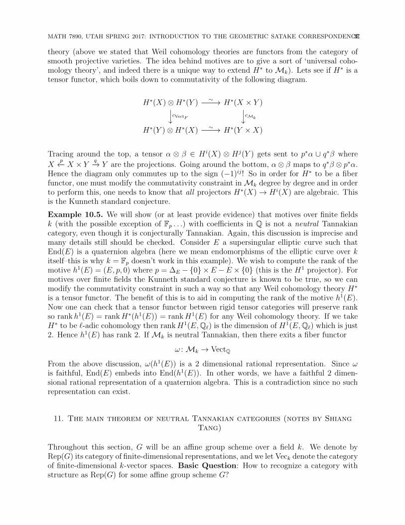
theory (above we stated that Weil cohomology theories are functors from the category ofsmooth projective varieties. The idea behind motives are to give a sort of ‘universal coho-mology theory’, and indeed there is a unique way to extend H∗ to Mk). Lets see if H∗ is atensor functor, which boils down to commutativity of the following diagram.
H∗(X)⊗H∗(Y ) H∗(X × Y )
H∗(Y )⊗H∗(X) H∗(Y ×X)
∼
cVectFcMk
∼
Tracing around the top, a tensor α ⊗ β ∈ H i(X) ⊗ Hj(Y ) gets sent to p∗α ∪ q∗β where
Xp←− X × Y q−→ Y are the projections. Going around the bottom, α⊗ β maps to q∗β ⊗ p∗α.
Hence the diagram only commutes up to the sign (−1)ij! So in order for H∗ to be a fiberfunctor, one must modify the commutativity constraint inMk degree by degree and in orderto perform this, one needs to know that all projectors H∗(X)→ H i(X) are algebraic. Thisis the Kunneth standard conjecture.
Example 10.5. We will show (or at least provide evidence) that motives over finite fieldsk (with the possible exception of Fp . . .) with coefficients in Q is not a neutral Tannakiancategory, even though it is conjecturally Tannakian. Again, this discussion is imprecise andmany details still should be checked. Consider E a supersingular elliptic curve such thatEnd(E) is a quaternion algebra (here we mean endomorphisms of the elliptic curve over kitself–this is why k = Fp doesn’t work in this example). We wish to compute the rank of themotive h1(E) = (E, p, 0) where p = ∆E −{0}×E −E ×{0} (this is the H1 projector). Formotives over finite fields the Kunneth standard conjecture is known to be true, so we canmodify the commutativity constraint in such a way so that any Weil cohomology theory H∗
is a tensor functor. The benefit of this is to aid in computing the rank of the motive h1(E).Now one can check that a tensor functor between rigid tensor categories will preserve rankso rankh1(E) = rankH∗(h1(E)) = rankH1(E) for any Weil cohomology theory. If we takeH∗ to be `-adic cohomology then rankH1(E,Q`) is the dimension of H1(E,Q`) which is just2. Hence h1(E) has rank 2. If Mk is neutral Tannakian, then there exits a fiber functor
ω : Mk → VectQ
From the above discussion, ω(h1(E)) is a 2 dimensional rational representation. Since ωis faithful, End(E) embeds into End(h1(E)). In other words, we have a faithful 2 dimen-sional rational representation of a quaternion algebra. This is a contradiction since no suchrepresentation can exist.
11. The main theorem of neutral Tannakian categories (notes by ShiangTang)
Throughout this section, G will be an affine group scheme over a field k. We denote byRep(G) its category of finite-dimensional representations, and we let Veck denote the categoryof finite-dimensional k-vector spaces. Basic Question: How to recognize a category withstructure as Rep(G) for some affine group scheme G?
38MATH 7890, UTAH SPRING 2017: INTRODUCTION TO THE GEOMETRIC SATAKE CORRESPONDENCE
First, we ask the opposite question: Fix a field k, and fix an affine group scheme G/k, towhat extent is G determined by Rep(G)?
Example 11.1. Let G be a finite group, regarded as a group scheme over C. Then Rep(G)is an abelian category, better yet a semi-simple category. As an abelian category,
Rep(G) ∼=⊕
W irreducible G-reps up to isomorphism
VecC
(Note that there are no nonzero maps between different summands.). This equivalence resultsby observing that for all V ∈ Rep(G),
V =⊕
irreducible G-reps W
(W -isotypic components of V )
(each component is canonically isomorphic to HomG(W,V )⊗W ), and we have
HomG(W⊗n,W⊗m) ∼= Mm,n(C).
Thus we see that the underlying abelian category Rep(G) does not remember G.
Key idea: We can recover G from the tensor abelian category Rep(G).
Exercise 11.2. (1) Find two non-isomorphic finite groups that have ”isomorphic char-acter tables”?
(2) Interpret part (1) in light of the key idea.
Proof. First, we make it precise what it means by two groups having isomorphic charactertables: Given a finite group G, denote by Conj(G) the set of conjugacy classes, and denoteby Char(G) the set of irreducible characters. We say two finite groups G,G′ have isomorphiccharacter table if there are bijections ϕ : Conj(G) → Conj(G′), α : Char(G) → Char(G′)such that ∀c ∈ Conj(G), ∀χ ∈ Char(G), χ(c) = α(χ)(φ(c)). For instance, it is easy to seethat D4 and Q8 have isomorphic character tables: both of which have four one-dimensionalcharacter and a unique irreducible two-dimensional character. However, there differencewill be seen immediately once we consider the alternating squares of their two-dimensionalrepresentations: one is isomorphic to the trivial character, the other is not. Therefore,Rep(D4) is not isomorphic to Rep(Q8) as abelian tensor categories, despite that D4 and Q8
have isomorphic character tables. �
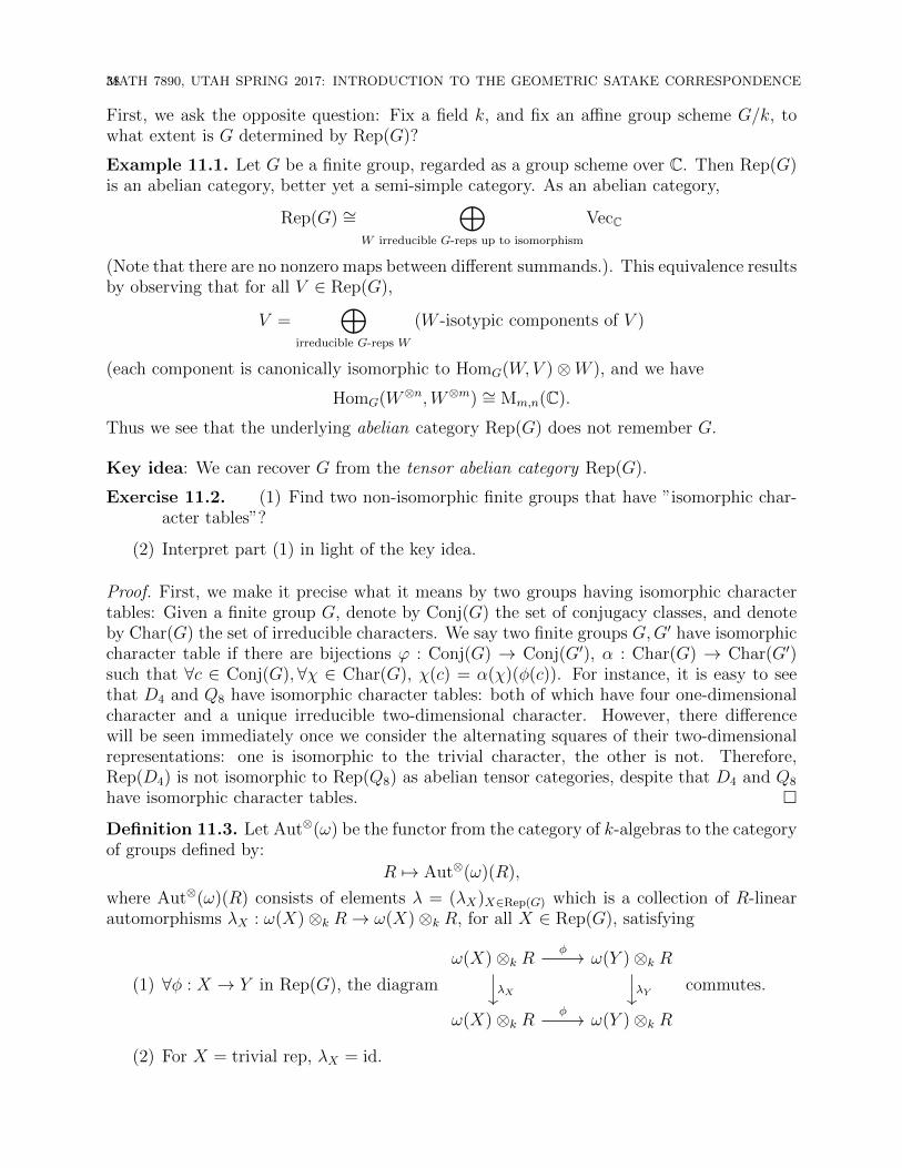
Definition 11.3. Let Aut⊗(ω) be the functor from the category of k-algebras to the categoryof groups defined by:
R 7→ Aut⊗(ω)(R),
where Aut⊗(ω)(R) consists of elements λ = (λX)X∈Rep(G) which is a collection of R-linearautomorphisms λX : ω(X)⊗k R→ ω(X)⊗k R, for all X ∈ Rep(G), satisfying
(1) ∀φ : X → Y in Rep(G), the diagram
ω(X)⊗k R ω(Y )⊗k R
ω(X)⊗k R ω(Y )⊗k R
φ
λX λY
φ
commutes.
(2) For X = trivial rep, λX = id.
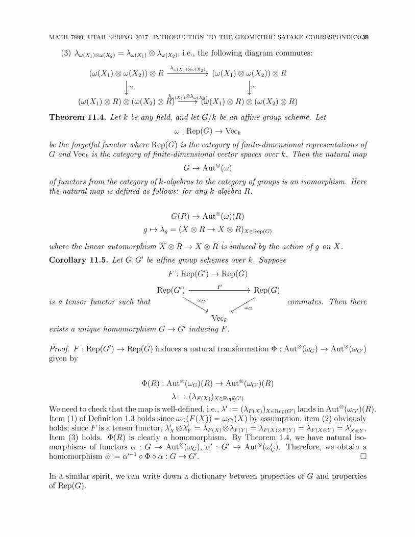
MATH 7890, UTAH SPRING 2017: INTRODUCTION TO THE GEOMETRIC SATAKE CORRESPONDENCE39
(3) λω(X1)⊗ω(X2) = λω(X1) ⊗ λω(X2), i.e., the following diagram commutes:
(ω(X1)⊗ ω(X2))⊗R (ω(X1)⊗ ω(X2))⊗R
(ω(X1)⊗R)⊗ (ω(X2)⊗R) (ω(X1)⊗R)⊗ (ω(X2)⊗R)
λω(X1)⊗ω(X2)
∼= ∼=λω(X1)⊗λω(X2)
Theorem 11.4. Let k be any field, and let G/k be an affine group scheme. Let
ω : Rep(G)→ Veck
be the forgetful functor where Rep(G) is the category of finite-dimensional representations ofG and Veck is the category of finite-dimensional vector spaces over k. Then the natural map
G→ Aut⊗(ω)
of functors from the category of k-algebras to the category of groups is an isomorphism. Herethe natural map is defined as follows: for any k-algebra R,
G(R)→ Aut⊗(ω)(R)
g 7→ λg = (X ⊗R→ X ⊗R)X∈Rep(G)
where the linear automorphism X ⊗R→ X ⊗R is induced by the action of g on X.
Corollary 11.5. Let G,G′ be affine group schemes over k. Suppose
F : Rep(G′)→ Rep(G)
is a tensor functor such that
Rep(G′) Rep(G)
Veck
ωG′
F
ωGcommutes. Then there
exists a unique homomorphism G→ G′ inducing F .
Proof. F : Rep(G′)→ Rep(G) induces a natural transformation Φ : Aut⊗(ωG)→ Aut⊗(ωG′)given by
Φ(R) : Aut⊗(ωG)(R)→ Aut⊗(ωG′)(R)
λ 7→ (λF (X))X∈Rep(G′)
We need to check that the map is well-defined, i.e., λ′ := (λF (X))X∈Rep(G′) lands in Aut⊗(ωG′)(R).Item (1) of Definition 1.3 holds since ωG(F (X)) = ωG′(X) by assumption; item (2) obviouslyholds; since F is a tensor functor, λ′X⊗λ′Y = λF (X)⊗λF (Y ) = λF (X)⊗F (Y ) = λF (X⊗Y ) = λ′X⊗Y ,Item (3) holds. Φ(R) is clearly a homomorphism. By Theorem 1.4, we have natural iso-morphisms of functors α : G → Aut⊗(ωG), α′ : G′ → Aut⊗(ω′G). Therefore, we obtain ahomomorphism φ := α′−1 ◦ Φ ◦ α : G→ G′. �
In a similar spirit, we can write down a dictionary between properties of G and propertiesof Rep(G).
40MATH 7890, UTAH SPRING 2017: INTRODUCTION TO THE GEOMETRIC SATAKE CORRESPONDENCE
Example 11.6. G is algebraic and of finite type over k is equivalent to Rep(G) has a tensorgenerator, i.e., there exists an object X in Rep(G) such that every object of Rep(G) isisomorphic to a subquotient of some⊕
m,n
(X⊗m ⊗ (X∨)⊗n
)This may fail when G is not algebraic, for instance, there is no such generator when G =Gal(Q/Q), the absolute Galois group, which is a profinite group, and is not algebraic.
Let us recall that our main task is going other way: having some category C that we wantto recognize as Rep(G).
Theorem 11.7 (Main Theorem). Let k be a field and let (C,⊗) be a rigid abelian tensorcategory with End(1) = k(1 is the unit object) and suppose that there exists a k-linear exactfaithful tensor functor (called a “fiber functor”)
ω : C → Veck
Then
(1) The functor Aut⊗(ω) from the category of k-algebras to the category of groups isrepresentable by an affine group scheme G over k.
(2) ω induces an equivalence
C ∼−→ Rep(G)
of tensor categories.
Proof. For a proof, see [Deligne-Milne, 2.11-2.16]. For part (2), ω induces a functor to Rep(G)since for all X ∈ C, ω(X) acquires a G-action from the isomorphism G ∼= Aut⊗(ω). �
12. p-adic Groups (notes by Kevin Childers)
12.1. Introduction. We’ve seen the finite dimensional algebraic representation theory ofcompact Lie groups and reductive algebraic groups. A natural next step in representationtheory is to study the representation theory of real Lie groups (e.g. SLn(R)) on Hilbertspaces (e.g. L2(SLn(R)) under the regular representation).
In parallel, we could study the representation theory of groups such as SLn(Qp). Both thereal representation theory and the p-adic representation theory arises naturally in numbertheory in the theory of modular forms.
A (semi-)classical perspective on modular forms, is to study the SL2(R)-representationL2(SL2(Z)\SL2(R)). A more modern approach is to package all completions of Q into thering of adeles:
AQ :=∗∏v
Qv = {(xv)v : xv ∈ Zv for all but finitely many v}.
Here v ranges through all places of Q and “∏∗” denotes a restricted product with respect to
Zv ⊂ Qv for v 6=∞ (the right hand side is the definition of restricted product in this case).
MATH 7890, UTAH SPRING 2017: INTRODUCTION TO THE GEOMETRIC SATAKE CORRESPONDENCE41
The ring of adeles is a locally compact group. Now we can study the SL2(AQ)-representationL2(SL2(Q)\SL2(AQ)).
12.2. Representations of GLn(Fp). To get a feel for what type of representations ofGLn(Qp) we will study, we will review the representation theory of GL2(Fp).
There are two types of easy representations of GL2(Fp). The first are the 1-dimensionalrepresentations factoring through the determinant map
GL2(Fp)det−−−→ F×p → C×.
The second, are the representations induced from the Borel subgroup, which we now review.
Let G = GL2(Fp) and
T =
(∗ 00 ∗
)⊂ B =
(∗ ∗0 ∗
)⊃ N =
(1 ∗0 1
)as subgroups of G. Let χ : T → C× be a character. Such a χ can be described as a pair ofcharacters χ1, χ2 : F×p → C×:
χ :
(t1 00 t2
)7→ χ1(t1)χ2(t2).
Such a χ extends to a character on the Borel B, and we obtain a G-representation
IndGB χ = {f : G→ C | f(bg) = χ(b)f(g) ∀b ∈ B, g ∈ G}.Notice that the dimension of IndGB χ is |G : B| = |P1(Fp)| = p+ 1.
The next question is: how do the representations induced in this way decompose into irre-ducible representations? Let
w =
(0 11 0
), ψw
(t1 00 t2
)= ψ
(t2 00 t1
)for any character ψ : T → C×. We have the following:
Proposition 12.1. With G, B, and T as above, let χ, ψ : T → C× be characters. Then
dim HomG(IndGB χ, IndGB ψ) =
0 if χ 6= ψ, ψw,
1 if χ = ψ or χ = ψw but ψ 6= ψw,
2 if χ = ψ = ψw.
In particular, IndGB χ is irreducible if and only if χ 6= χw. If χ = χw, then IndGB χ is thedirect sum of two distinct irreducible representations.
Example 12.2. We give an example of the reducible case. The induction of the trivialrepresentation is just
IndGB(1B) = {f : B\G→ C}.The constant functions give a subrepresentation, isomorphic to the trivial representation ofG. We have an exact sequence
0→ 1G → IndGB(1B)→ St→ 0.
The quotient is an irreducible representation called the Steinberg representation.
42MATH 7890, UTAH SPRING 2017: INTRODUCTION TO THE GEOMETRIC SATAKE CORRESPONDENCE
Proof.
HomG(IndGB χ, IndGB(ψ)) = HomB(IndGB χ|B, ψ)
= HomB(⊕
w′∈{1,w}IndB
B∩Bw′ χw′ , ψ)
= HomB(χ, ψ)⊕ HomB(IndBT χw, ψ)
= HomT (χ, ψ)⊕ HomT (χw, ψ).
The first and last equality are Frobenius reciprocity, and the second inequality is the induction-restriction formula. Here we are using the fact that 1, w are a set of representatives forB\G/B, and B ∩Bw = T (Bw consists of lower triangular matrices). �
We will be studying the analogue of these representations on p-adic groups (e.g. GL2(Qp)).
Remark 12.3. We’ve now classified the easy representations. For the rest, we take a non-splitmaximal torus in G, induce the representations, and decompose the result. These are calledthe cuspidal representations.
Example 12.4. As an example of a non-split maximal torus, as in Remark 12.3, choosea basis of Fp2 over Fp. Then we get a map Fp2 → M2(Fp) by mapping α to the matrixrepresenting “multiplication by α” with respect to the chosen basis. Taking units gives amap F×p2 ↪→ GL2(Fp), which is the inclusion of a maximal torus.
12.3. Locally profinite groups. Let K denote a non-archimedean local field (i.e. a finiteextension of Fp((t)) or Qp). Our focus will be the representation theory of connected reductivegroups G/K. Of course, some of the results hold more generally.
Definition 12.5. A locally profinite group is a Hausdorff topological group, such thatevery open neighborhood of the identity contains a compact open subgroup.
Exercise 12.6. Let G be a Hausdorff topological group. Show that G is profinite if andonly if every open neighborhood of the identity contains a compact open normal subgroup.
Example 12.7. G = GLn(Qp) is locally profinite. A basis of compact open subgroups atthe identity is given by
{1 + pNMn(Zp) | N ≥ 1}.
The basic class of representations of a locally profinite group G is the following.
Definition 12.8.
(1) Let G be a locally profinite group. A smooth representation of G is a homomor-phism π : G → AutC(V ) for some C-vector space V such that V =
⋃K V
K , whereK ranges over compact open subgroups K of G. In other words, every vector v ∈ Vhas open stabilizer.
(2) A smooth representation is admissible if V K is finite dimensional for all compactopen subgroups K of G.
Let M(G) denote the category of smooth representations of a locally profinite group G.
Exercise 12.9. Show that M(G) is an abelian category.
MATH 7890, UTAH SPRING 2017: INTRODUCTION TO THE GEOMETRIC SATAKE CORRESPONDENCE43
Example 12.10. A 1-dimensional smooth representation of a locally profinite group G is acharacter χ : G→ C× such that χ is trivial on a compact open subgroup (i.e. kerχ is open).For instance, if G = Q×p , characters χ : Q×p → C× with χ|1+pnZp trivial for some n ≥ 1 aresmooth. If χ : Q×p → C× is trivial on Z×p , then χ is completely determined by χ(p). Thesecharacters are called unramified.
However, the typical examples of interest to us will be infinite dimensional, since G willtypically be non-abelian.
Exercise 12.11. What are the smooth representations when G is a compact group, forexample G = GL2(Zp)?
Representations π ∈ M(G) are not necessarily semi-simple. However, we do have the fol-lowing.
Lemma 12.12. Let π ∈M(G) and let K be a compact open subgroup of G. Then
(1) π|K is semi-simple, and
(2) π 7→ πK is an exact functor.
Proof of (1). Let v ∈ V . Since V is smooth, exercise 12.6 implies v ∈ V K′ for some com-pact open normal subgroup K ′. By compactness, K ′ has finite index in K. Thus theK-representation generated by v is finite dimensional (and semisimple, since it is a repre-sentation of the finite group K/K ′). So V |K is the sum of irreducible K-representations. Astandard Zorn’s Lemma argument shows this implies that V |K is a direct sum of irreducibleK-representations. �
12.4. The induction functor. In order to construct representations of a profinite groupG, we want an induction functor from representations of a closed subgroup H.
Lemma 12.13 (Frobenius reciprocity). The restriction functorM(G)→M(H) has a rightadjoint, denoted by IndGH :M(H)→M(G).
In finite group theory, the definition of the induction functor for an H-representation π is
IndGH π = {f : G→ π | f(hg) = π(h)f(g) ∀h ∈ H, g ∈ G}.The problem with this definition in our setting is that this will not in general producesmooth representations. However, there is a smoothing functor from the category of all G-representations to the categoryM(G), which sends a representation V to
⋃K V
K , where Kranges over compact open subgroups. Applying the smoothing functor to the above definitiongives the
Definition 12.14. Let G be a locally profinite group and H a closed subgroup. Let π ∈M(G). We define IndGH π ∈M(H) to be
IndGH π =
{f : G→ π
∣∣∣∣ f(hg) = π(h)f(g) ∀h ∈ H, g ∈ G, and∀g ∈ G∃ a compact opensubgroup K such that f(gk) = f(g) ∀k ∈ K
}.
With this definition, the proof of Frobenius reciprocity is the same as in the finite groupcase, with an additional check of the topological conditions.
44MATH 7890, UTAH SPRING 2017: INTRODUCTION TO THE GEOMETRIC SATAKE CORRESPONDENCE
Exercise 12.15. Show that IndGH :M(H)→M(G) is an exact functor.
Example 12.16. We will now parallel the constructions given in subsection 12.2 on thelocally profinite group G = GL2(Qp). Let B and T denote the borel and maximal torus,parallel to the finite example.
For any smooth character χ : T → C× we form a smooth G-representation IndGB χ (this willbe infinite dimensional). A similar argument to Proposition 12.1 shows
(1) If χ 6= χw, IndGB χ is irreducible.
(2) If χ = χw, IndGB χ fits in an exact sequence with two smooth irreducible representa-tions. For example, we have an exact sequence
0→ 1G → IndGB(1B)→ St→ 0.
The sequence in (2) does not split. The problem we run into is that IndGB is not a left adjointto restriction, as opposed to the finite group setting.
12.5. Representation theory of reductive groups over local fields. Let F denote anon-archimedean local field, and let O denote the ring of integers of F . Let G/O denote asplit, connected, reductive group. We will also abusively write G for G(F ). Let π ∈ M(G)be irreducible and admissible. Consider the condition that πG(O) 6= 0.
Remark 12.17. In the global setting this happens almost everywhere locally. For example,if F is a number field, an automorphic representation of GL1 over F is a continuouscharacter χ : A×F/F× → C×. For any such χ, there exists a finite set S of primes such that χis trivial on O×Fv for all v 6∈ S. The reason for this is that
∏v-∞O
×Fv
is a profinite group, and
any continuous homomorphism from a profinite group to C× must factor through a finitequotient. There exists an analogous result for automorphic representations on higher rankgroups.
Definition 12.18. Back in the setting described before the remark, fix a compact opensubgroup K of G. We say π ∈M(G) is K-spherical if π is irreducible and πK 6= 0.
If we let K = G(O), do K-spherical representations exist? The answer is yes, and toconstruct them we use the Iwasawa decomposition.
Lemma 12.19 (Iwasawa decomposition). With notation as above, if G is split, then G(F ) =B(F )G(O).
Proof for GLn. I claim it suffices to show that G(O) surjects onto G/B(O). Recall that G/Bis a projective variety, and as such we can “clear denominators” in projective coordinates toget G/B(O) = G/B(F ). Now G(F )→ G/B(F ) is surjective with kernel B(F ), so surjectionof G(O) onto G/B(O) = G/B(F ) will imply G(F ) = B(F )G(O). Now a flag in G/B(O)must look like
0 ⊂ L1 ⊂ L2 ⊂ · · · ⊂ Ln = Rn,
where Li is a free R-module of rank i, which is a direct summand of Ln. In particular, sucha flag is in the image of the map G(O)→ G/B(O). �
MATH 7890, UTAH SPRING 2017: INTRODUCTION TO THE GEOMETRIC SATAKE CORRESPONDENCE45
Consider a character χ : T (F )/T (O)→ C×. I claim that IndGB(χ)K 6= 0. To see this, defineϕχ ∈ IndGB χ by ϕχ(bk) = χ(b), where bk ∈ B(F )G(O) = G(F ). In fact, this definition isforced upon us. Note that this is well-defined, since χ|B∩K is trivial.
Remark 12.20. This example does not quite produce K-spherical representations, sinceIndGB χ is not necessarily irreducible. But as for the finite group case of subsection 12.2,IndGB χ will be irreducible if and only if χ 6= χw. We will not provide a proof of this.
If we pursued this remark further, we would arrive at the
Theorem 12.21 (Borel-Matsumoto-Casselman). With notation as above,
(1) Any unramified principal series IndGB χ with χ unramified has a unique K = G(O)-spherical subquotient.
(2) Any K-spherical representation embeds into an unramified principle series.
This theorem provides one way to classify K-spherical representations for K = G(O). Laterwe will give a different classification, which is more directly related to the Satake isomor-phism.
13. Studying K-spherical representations via Hecke algebras (Notes bySabine Lang)
For the time being, we can take G any locally profinite group, and K any compact opensubgroup of G.
Recall that in finite group theory, one studies representations of G by viewing them as C[G]-representations. We can identify C[G] ' Maps(G,C), which is an identification of C-algebrasgiven by ∑
g∈G
agg → (f : G→ C, f(g) = ag).
The multiplication on Maps(G,C) is the convolution of functions, i.e., for f1, f2 : G→ C, wehave (f1 ∗ f2)(g) =
∑x∈G f1(x)f2(x−1g). Now we will mimic this for locally profinite groups.
Definition 13.1. The Hecke algebraH(G) of G is the C-algebra of functions f : G→ C thatare locally constant with compact support. We write H(G) = C∞c (G). The multiplication isgiven by
(f1 ∗ f2)(g) =
∫G
f1(x)f2(x−1g)dµG(x), for all g ∈ G, f1, f2 ∈ C∞c (G),
where µG is a Haar measure on G (more details on Haar measure will come later in thenotes).
Remark 13.2. For any f ∈ C∞c (G), there exists a compact open subgroup K < G such thatf is K-bi-invariant (i.e., f factors through K\G/K).
Proof. Because f is locally constant, for every x ∈ G there exists a neighborhood Ux of x suchthat f |Ux= f(x). Since G is locally profinite, there exists a compact open subgroup Kx such
that xKx ⊂ Ux and Kxx ⊂ Ux (we can take Kx with Kxx ⊂ Ux, Kx with xKx ⊂ Ux and we
46MATH 7890, UTAH SPRING 2017: INTRODUCTION TO THE GEOMETRIC SATAKE CORRESPONDENCE
define Kx = Kx∩Kx). Write G as G = ∪x∈GxKx = ∪x∈GKxx. Since f has compact support,we can extract finite subcovers of the support of f , so supp(f) = ∪i=1,...,nxiKxi ∩ supp(f) =∪j=1,...,mKyjyj ∩ supp(f). By choosing K = ∩i=1,...,nKxi
⋂∩j=1,...,mKyj , we observe that f is
K-bi-invariant. �
From the remark, we can write H(G) = ∪KH(G,K) where we take the union over all thecompact open subgroups K of G. Here H(G,K) (also written HK) denotes the subalgebra(check this!) of K-bi-invariant functions in H(G).
13.1. Overview of the translation from smooth G-representations to smooth H(G)-modules. We will prove the two following results (smooth H(G)-modules will be definedlater in the notes):
(1) There is an equivalence of categories
M(G)→ {smooth H(G)-modules}.
(2) For all K, there is a bijection
{Irreducible smooth G-rep. π with πK 6= 0} /' → {Simple HK-modules} /' .
Now we can make this more precise. First, we will do some preliminaries on integration.Recall that any locally compact (Hausdorff) topological group has a unique (up to scaling)left- (or right-) invariant Haar measure, i.e., a functional I : Cc(G)→ R such that
(1) I(f) ≥ 0 for f ≥ 0,
(2) I(λg · f) = I(f) for all g ∈ G and f ∈ Cc(G), where λg denotes the left-regularrepresentation of G on Cc(G).
We can rewrite the second condition as∫Gf(g−1x)dµ(x) =
∫Gf(x)dµ(x). We also introduce
the notation ρg for the right-regular representation of G on Cc(G).
But with G locally profinite, we just use the following bare-hands approach : a left-invariantHaar measure will be such a functional I defined on C∞c (G) (and not the whole space Cc(G)),and it is constructed as follows:
• Fix K < G a compact open subgroup.
• Declare I(1K) = 1 for 1K the characteristic function of K (normalization).
• For any K ′ ⊂ K, write K as a finite disjoint union K = taiK ′ and the left-invariance
forces I(1K′) =1
[K : K ′]. Likewise, left-invariance forces I(1gK′) =
1
[K : K ′]for all
g ∈ G and for all such K ′.
• Extend linearly.
This will force a unique construction of a left-invariant functional I : C∞c (G)→ R.
MATH 7890, UTAH SPRING 2017: INTRODUCTION TO THE GEOMETRIC SATAKE CORRESPONDENCE47
13.2. Relation between left and right Haar measures. Let I be a left-invariant Haarmeasure, written as I(f) =
∫Gf(g)dµG(g). Then for any g ∈ G, we consider I(ρg · f) =∫
Gf(xg)dµG(x). Since left and right regular representations commute, the map that sends
f to I(ρg · f) is also a left-invariant Haar measure. By uniqueness (up to scaling) of a left-invariant Haar measure on G, there exists δG(g) ∈ R>0 such that δG(g)I(ρg · f) = I(f) forall f .
We can check that δG : G→ R>0 is a smooth character : we apply it to g1 · g2 as follows :
I(f) = δG(g1 · g2)I(ρg1·g2f) = δG(g1 · g2)I(ρg1ρg2f)
= δG(g1 · g2)δG(g1)−1I(ρg2f) = δG(g1 · g2)δG(g1)−1δG(g2)−1I(f),
so we obtain δG(g1 · g2) = δG(g1)δG(g2). To check that δ is smooth, fix any compact opensubgroup K. For k ∈ K,
I(1K) = I(ρk1K) = δG(k)−1I(1K),
so δG is trivial on K (note that if we take a subgroup K of G which is not compact open,then 1K is not an element of C∞c (G), so this argument does not apply). We call δG themodulus character of G.
Example 13.3. • As we have just seen, if G is compact, then δG is trivial.
• If G = G(F ) is reductive, then δG is trivial.
• A typical example with δG non-trivial arises when we take G to be a Borel subgroup.
Moreover, δG measures the difference between the left- and right-invariant Haar measures.Define I ′(f) = I(δ−1
G · f). Then I ′ is a right-invariant Haar measure :
I ′(ρg · f) = I(δ−1G · ρg · f) = I(δG(g) · ρg(δ−1
G · f)) = δG(g)I(ρg(δ−1G · f)) = I(δ−1
G · f) = I ′(f).
Now we return to the setting of interest with F a non-archimedean local field, O its ringof integers, G = G(F ) and K = G(O). One of our aims is to classify the K-sphericalrepresentations of G.
How? One way, as in Theorem 12.21, is to understand how to find all K-spherical represen-tations inside IndGB(χ) for χ : T (F )/T (O) → C×. We will take a less explicit approach tothe classification, but one that arises directly from the Satake isomorphism. We first pointout one more thing about unramified principal series that was omitted last time.
Remark 13.4. (A subtlety arising from the failure of unimodularity of B.) We saw thatIndGB(χ)K is 1-dimensional in this case but IndGB(χ) is not necessarily irreducible. For exam-ple, for G = GL2(F ), we have the short exact sequence
0→ 1→ IndGB(1)→ St → 0,
which does not split, and when we dualize it we get
0→ St → IndGB(1)∨ → 1→ 0,
where St is the Steinberg representation. Here we do NOT have IndGB(1)∨ ' IndGB(1). We
have to be careful : in general, IndGB(χ)∨ ' IndGB(χ−1 · δ−1
B ).
48MATH 7890, UTAH SPRING 2017: INTRODUCTION TO THE GEOMETRIC SATAKE CORRESPONDENCE
Pursuing this, we get that IndGB(χ) is irreducible either when χ1 = χ2 or when χ1 = χ2· | |2,where χ = (χ1, χ2). We have a G-equivariant pairing
IndGB(χ)× IndGB(χ−1δ−1B )→ C
given by
(f1, f2) 7→∫B\G
f1(g)f2(g)dµB\G(g),
which implies that IndGB(χ)∨ ' IndGB(χ−1 · δ−1
B ). The subtelty here is that we can onlydefine a right-invariant measure µB\G on the set {f : G→ C | f(bg) = δB(b)−1f(g), f locallyconstant with compact support}.Remark 13.5. Here ( )∨ means the smooth dual, i.e., the smooth vectors in the algebraicdual.
Now, we need to learn how to integrate over B for B a Borel subgroup. (Note that thefollowing discussion works equally well for a parabolic P = M nN instead of B.)
We write B as the semidirect product B = T n N , which is isomorphic to T × N as atopological space. But T and N are both unimodular (i.e., δT and δN are trivial). Fix bothleft- and right-invariant Haar measures IN and IT on C∞c (N) and C∞c (T ). We use them todefine a left-invariant Haar measure in B by IB(f) =“
∫Bf(b)db =
∫T
(∫Nf(tn)dn)dt”. The
following commutative diagram makes sense of this notation :
C∞c (T )⊗ C∞c (N) C∞c (T )
C∞c (B) C
IN
' IT
IB
and the isomorphism
C∞c (T )⊗ C∞c (N)→ C∞c (B)
is given by
φ⊗ ψ 7→ (b = tn 7→ φ(t)ψ(n)).
We observe that IB is left-invariant. It suffices to show that IB(λ(t0,n0)−1φ⊗ψ) = IB(φ⊗ψ),for all φ ∈ C∞c (T ) and ψ ∈ C∞c (N). Analyzing λ(t0,n0)−1φ⊗ ψ, we get
(λ(t0,n0)−1φ⊗ ψ)(t, n) = (φ⊗ ψ)((t0, n0) · (t, n)) = (φ⊗ ψ)(t0t, t−1n0tn) = φ(t0t)ψ(t−1n0tn).
Using the fact that t−1n0t is an element of N , and the invariance of both IN and IT , weobtain IB(λ(t0,n0)−1φ⊗ ψ) = IB(φ⊗ ψ).
We want to use this definition of the left-invariant measure IB to calculate the correspondingmodulus character δB. Recall that it is defined by δB(b)IB(ρb ·f) = IB(f). Fix now b0 = t0n0.We compute
IB(ρb0 · f) =
∫T
∫N
f(tnt0n0)dndt =
∫T
∫N
f(tt0t−10 nt0n0)dndt,
MATH 7890, UTAH SPRING 2017: INTRODUCTION TO THE GEOMETRIC SATAKE CORRESPONDENCE49
and writing f = φ⊗ ψ we get
IB(ρb0 · f) =
∫T
φ(tt0)dt
∫N
ψ(t−10 nt0n0)dn = IT (φ)
∫N
ψ(t−10 nt0)dn,
using the fact that both IT and IN are unimodular. Note that we cannot use the invarianceof IN to simplify
∫Nψ(t−1
0 nt0)dn since we are multiplying by elements of T , and not elementsof N .
Remark 13.6. For a fixed t0 ∈ T , the functional sending ψ to∫Nψ(t−1
0 nt0)dn is a Haar
measure on N . By unicity (up to scaling) of a Haar measure, we obtain∫Nψ(t−1
0 nt0)dn =cst(t0)IN(ψ). Here cst(t0) does not depend on ψ, so we can choose any ψ we like to computethis quantity.
We observe that IB(ρb0 · f) = IT (φ)cst(t0)IN(ψ) = cst(t0)IB(f), so δB(b0) = cst(t0)−1.
Example 13.7. Take G = GL2(F ), t =
(t1
t2
)and ψ = 1N(O). In this case, N(O) =
{(
1 x0 1
)| x ∈ O}. We may assume the normalization IN(1N(O)) = 1. We want to compute∫
G(F )1N(O)(
(1 x t2
t10 1
))dx =
∫F1 t1t2O(x)dx. So the question is : given that O has volume 1,
what volume does t1t2O have?
Answer : | t1t2|, where | | is normalized as (# O
πO )−ν(
t1t2
)with ν : O � Z. So in this case,
δB(
(t1 ∗0 t2
)) = | t1
t2|−1 = | t2
t1|.
More generally, for a group G, we obtain δB(t) = | det(Ad(t) |n)|−1.
13.3. Back to Hecke algebras. For now, G can be any locally profinite group. Recall :
H(G) = C∞c (G) = ∪KH(G,K),
where the union is taken over the compact open subgroups K of G, and H(G,K) = HK isthe subspace of K-bi-invariant functions. We observe that HK is a subalgebra of H(G), andHK = eK ∗ H(G) ∗ eK where eK = 1K
vol(K). We can check that the eK are idempotents : for
g ∈ G, we have
(eK ∗ eK)(g) =
∫G
eK(x)eK(x−1g)dµG(x) =1
vol(K)
∫K
eK(x−1g)dµG.
Since we consider now x ∈ K, this expression is zero if x−1g /∈ K, i.e., if g /∈ K. In the casewhere g ∈ K, we have
(eK ∗ eK)(g) =1
vol(K)
∫K
eK(x−1g)dµG = (1
vol(K))2vol(K) =
1
vol(K),
so we conclude that eK ∗ eK = 1K
vol(K)= eK .
50MATH 7890, UTAH SPRING 2017: INTRODUCTION TO THE GEOMETRIC SATAKE CORRESPONDENCE
13.4. Construction of the equivalence M(G) → { smooth H(G) − modules}. Let(π, V ) ∈M(G). Let f ∈ H(G), and let v ∈ V . We define an action of H(G) on V by
π(f) · v =
∫G
f(g)π(g)(v)dg.
Exercise 13.8. The expression π(f) · v can be rewritten as a finite sum (Hint : use the factthat f is locally constant with compact support, and that π is a smooth representation.)
Exercise 13.9. This defines an action. Note that there is no unit in H(G), so there isno unit condition to check : we only want the associativity. So we need to check thatπ(f1 ∗ f2) · v = π(f1) · (π(f2) · v), which can be done by developing both sides explicitely andusing the left-invariance of the Haar measure on G.
What kinds of H(G)-modules do we obtain?
Definition 13.10. An H(G)-module V is smooth if for all v ∈ V , there exists a compactopen subgroup K of G such that eK · v = v.
Proposition 13.11. The map M(G) → { smooth H(G) − modules} is an equivalence ofcategories.
Proof. First, we need to check that (π, V ) ∈ M(G) gives a smooth H(G)-module: we knowthat for each v ∈ V , there exists a compact open subgroup K of G with πK 6= 0. Then wecan check that π(eK) · v =
∫G
1K
vol(K)(g)π(g)(v)dg =
∫K
1vol(K)
π(g)(v)dg = π(g)(v) = v since
g ∈ K from the previous equality and v is an element of πK .
Then, we need to give a quasi-inverse map. Given a smooth H(G)-module V , let v ∈ V andg ∈ G. We have to define π(g). Choose any K such that eK · v = v (such a K exists bysmoothness of V ). Then we set π(g) · v = egK · v. We need to check that this is well-defined.
Let K ′ be another subgroup with eK′ · v = v. We can reduce to the case where K ′ ⊂ K.Now if K ′ is a subgroup of K, we have
(egK′ ∗ eK)(y) =
∫G
1gK′(x)
vol(gK ′)
1K(x−1y)
vol(K)dx =
∫gK′
1K(x−1y)
vol(gK ′)vol(K)dx,
so we have here x−1 ∈ K ′g−1 and we get
(egK′ ∗ eK)(y) = 0 if y /∈ gK,
(egK′ ∗ eK)(y) =1
vol(K)=
1
vol(gK)if y ∈ gK,
so we have shown that egK′ ∗ eK = egK .
In particular, egK′ · v = (egK′ ∗ eK) · v = egK · v, since eK · v = v by choice of K. So this is awell-defined action, and checking the equivalence is now easy. �
Our next goal is to show that we have the following bijection, for any K:
{Irreducible smooth G-rep. (π, V ) with πK 6= 0} /' → {Irreducible HK-modules} /'induced by
V 7→ V K .
MATH 7890, UTAH SPRING 2017: INTRODUCTION TO THE GEOMETRIC SATAKE CORRESPONDENCE51
Lemma 13.12. For all (π, V ) ∈ M(G), π(eK) : V → V K is a projection. In particular,HK = eK ∗ H(G) ∗ eK acts on V K.
Proof. We already saw that eK is an idempotent. The next exercises shows that the imageof V by π(eK) lies indeed in V K and concludes the proof. �
Exercise 13.13. Check that for all k ∈ K, we have π(k) · π(eK)(v) = π(eK)(v). (Hint: usea change of variable.)
Proposition 13.14. The map sending V to V K is a bijection on isomorphism classes ofirreducible objects, as claimed.
Proof. First, we check that if (π, V ) is irreducible, then V K is an irreducible HK-module.Since we consider our map as
{Irreducible smooth G-rep. (π, V ) with πK 6= 0} /' → {Irreducible HK-modules} /' ,then πK 6= 0. Suppose 0 ( M ( V K is a proper HK-submodule. Then by definition ofM ⊂ V K we have M = π(eK)M , and H(G)M = V by the previous equivalence and theirreducibility of V . So we get
V K = π(eK) · V = π(eK)H(G) ·M = π(eK)H(G)π(eK) ·M = HK ·M = M,
which is a contradiction since we assumed M ( V K . This implies that V K is irreducible.
Now we construct a quasi-inverse. Given an irreducible HK-module M , then there exists anideal I of HK such that M ' HK /I . We now consider I ⊂ HK ⊂ H(G) and form the H(G)-
submodule generated by I inside H(G), call it I. We also denote by HK the H(G)-module
generated by HK . The quotient HK /I is a H(G)-module but it might be too big. Using
Zorn’s lemma, we can take V to be any non-zero irreducible quotient, i.e., HK /I � V.
First, we check that V K is non-zero : we apply ( )K to the short exact sequence
0→ U → HK /I → V → 0
and by exactness of ( )K we have the short exact sequence
0→ UK → (HK /I )K → V K → 0.
But we know that (HK /I )K = HK /I = M by definition. So the exact sequence is
0→ UK →M → V K → 0.
If V K = 0 we obtain UK = M , and therefore U generates HK /I . But this implies thatV = 0, which is a contradiction. So we have V K 6= 0 and by irreducibility of M we see thatV K = M as desired. �
13.5. A couple of loose ends. For G a locally profinite group, if G/K is countable forsome compact open K then :
(1) Any smooth (π, V ) ∈M(G) has countable dimension.
(2) Schur’s lemme holds : if (π, V ) is irreducible, then EndG(π) = C.
52MATH 7890, UTAH SPRING 2017: INTRODUCTION TO THE GEOMETRIC SATAKE CORRESPONDENCE
Proof. We will leave (1) as an exercise and prove (2). Since π is irreducible, EndG(π) is adivison algebra over C, not a priori finite dimensional. Fix v ∈ V \{0}. Any φ ∈ EndG(π)is then determined by φ(v) since v generates (π, V ). So by (1), EndG(π) has countabledimension. If φ /∈ C, then we consider (note that C(φ) is a field since EndG(π) is a divisionalgebra)
{ 1
φ− a| a ∈ C} ⊂ C(φ).
All the elements 1φ−a are linearly independant over C, and there are uncountably many of
these. So EndG(π) would have uncountable dimension, which is a contradiction. This showsthat EndG(π) = C. �
14. Statement of classical Satake isomorphism
Shiang Tang
Recall that if K is a compact open subgroup of G that is locally profinite, the set of isomor-phism classes of smooth irreducible G-representations π such that πK 6= 0 is equivalent tothe set of isomorphism classes of irreducible HK-modules πK . The case of basic interest tous is the following situation: F is a local field with ring of integers O and a uniformizer $.G is a split connected reductive group scheme defined over O, G = G(F ), K = G(O). Inthis case, HK can be explicitly described.
The following theorem gives us the first information about HK .
Theorem 14.1 (Cartan decomposition). For G,K as above,
G =⊔
λ∈X∗(T)/W
Kλ($)K
(If we choose B ⊃ T , then we get X∗(T )/W = X∗(T )+.)
Proof for GLn. It uses the structure theory of modules over PID. Let V = F n ⊃ Λ =On = ⊕ni=1ei. For g ∈ GLn(F ), consider the translated lattice g(Λ), these two lattices arecommensurable so ∃N , such that $Ng(Λ) ⊂ Λ. By theory of finite-generated O-modules, ∃a basis f1, · · · , fn of Λ and integers a1 ≥ · · · ≥ an such that $a1f1, · · · , $anfn form a basisof $Ng(Λ) and hence $a1−Nf1, · · · , $an−Nfn form a basis of g(Λ). Let B be the matrixof g under the basis f1, · · · , fn of Λ, so g = SBS−1 for some S ∈ GLn(O). Since both ofgf1, · · · , gfn and $a1−Nf1, · · · , $an−Nfn are O-bases of g(Λ), there exists C ∈ GLn(O) suchthat B = diag($a1−N , · · · , $an−N) · C and so g = S · diag($a1−N , · · · , $an−N) · CS−1 ∈Kdiag($a1−N , · · · , $an−N)K. �
Corollary 14.2. HK has a basis given by {1Kλ($)K}λ∈X∗(T )+.
Theorem 14.3 (Satake Isomorphism). There is an algebra isomorphism
HK → HWT (O)
where HT (O) = H(T (F ), T (O)), given by
f 7→ (Sf)(t) = δ(t)1/2
∫N
f(tn)dn
MATH 7890, UTAH SPRING 2017: INTRODUCTION TO THE GEOMETRIC SATAKE CORRESPONDENCE53
where δ(t) = | det(Ad(t)|n)|−1.
We make the following important remarks.
Remark 14.4. RHS=HWT (O).
C[X∗(T )] ∼= C∞c (T (F )/T (O))
[µ] 7→ 1µ($)T (O)
is an isomorphism of algebras. So
HK → HWT (O)∼= C[X∗(T )]W = C[X∗(T∨)]W = R(G∨)⊗ C
The isomorphism HK∼= R(G∨)⊗ C is what geometric Satake will categorify.
Remark 14.5. HK is commutative!
Remark 14.6. Since HK = HWT (O) is commutative, the following sets are in bijections:
{simple HK-modules} ↔ {1-dimensional representations of HWT (O)} ↔
{C-algebra homomorphisms: HWT (O) = C[X∗(T∨)]W = OT∨/W → C} ↔ (T∨/W )(C)
↔ {semisimple conjugacy classes in G∨}The last bijection holds since every semisimple element of G∨ is contained in some maximaltorus, and all maximal tori are G∨-conjugate.
The point of Remark 1.6 is that it induces the unramified case of the local Langlands program,on which we give a short introduction: Let Π(G) be the set of irreducible smooth admissibleG-representations up to isomorphisms (the ”automorphic side”). Let Φ(G) be the set ofL-parameters for G up to equivalence (the ”Galois side”). To define L-parameter, we startwith the definition of Weil group:
Definition 14.7 (Weil group). Given a non-archimedean local field F , we have the followingexact sequence
1→ IF → Gal(F /F )→ Gal(kF/kF )→ 1
where kF is the residue field of F and Gal(kF/kF ) ∼= Z is generated by the Frobenius mapFrob : x 7→ x|kF |, IF is the inertia group. Define WF to be the preimage of Z =< Frob >, soit fits into an exact sequence
1→ IF → WF → Z→ 0
This defines WF as a group. As a topological group, we declare IF to be an open subgroupwith its natural profinite topology. Note that WF is not a profinite group.
Definition 14.8. An L-parameter for G is a pair (r,N) where
r : WF → G∨(C)
is a continuous homomorphism and where N is a nilpotent element in Lie(G) such that
r(g)Nr(g)−1 = qmN
where the image of g in Gal(kF/kF ) is Frobm.
54MATH 7890, UTAH SPRING 2017: INTRODUCTION TO THE GEOMETRIC SATAKE CORRESPONDENCE
Now we define Φ(G) to be
{(r,N)|r(Frob) is semisimple}/ ∼=
We give a very crude form of Local Langlands Correspondence: There is a map
LLG : Π(G)→ Φ(G)
all of whose fibers are finite non-empty subsets (”L-packets”) of Π(G) and satisfying variousrequirements without which the statement will not be meaningful. We omit the details here.
Example 14.9. For G = GLn such a correspondence is a theorem of Harris-Taylor, in whichcase LLG is a bijection, and one way of characterizing the bijection is via L-functions andepsilon factors. The case of a general reductive group is still wide open.
Example 14.10 (Unramified LLC). Let Φunr(G) be the set of equivalent classes of unrami-fied homomorphisms γ : WF/IF → G∨(C) such that r(Frob) is semisimple. It is in bijectionwith the set of semisimple conjugacy classes in G∨(C).
Let Πunr(G) be the set of irreducible smooth G-representations π such that there exists aconnected reductive group scheme G defined over O with generic fiber G and πG(O) 6= 0.(Note that in general there may exist more than one such reductive integral model G).
The unramified LLC is then the map
Πunr(G)→ Φunr(G)
induced by the Satake isomorphism. To be precise, let π ∈ Πunr(G), with G/O the reductive
group scheme such that πG(O) 6= 0. Then the Satake isomorphismHG(O)∼−→ HW
T (O) associates
to the HG(O)-module πG(O) a semisimple conjugacy class in G∨(C), and thus an element ofΦunr(G).
Remark 14.11 (To Example 1.10). Even in the unramified setting, we can have L-packets thatare not singletons. For instance, we can have smooth irreducible unramified representationπ on GL2(Qp) such that π|SL2(Qp) is not irreducible; in this case the constituents of therestriction form an L-packet. For example, the irreducible unramified representation
IndGL2(Qp)B (ε| · |1/2 ⊗ | · |−1/2),
where ε is the unramified character
Qp/Zp → {±1}p 7→ −1
, is reducible when restricted to SL2(Qp).
Back to Satake isomorphismS : HK → R(G∨)⊗Z C
LHS has a basis cλ = 1Kλ($)K , λ ∈ X∗(T )+, RHS has a basis ch(V (λ)), λ ∈ X∗(T )+ whereV (λ) is the highest weight representation corresponding to λ.
Motivating Question: What in HK maps to ch(V (λ))? A full understanding will comefrom geometric Satake.
Let us do some warm-up calculation before moving to the proof of Satake Isomorphism.
MATH 7890, UTAH SPRING 2017: INTRODUCTION TO THE GEOMETRIC SATAKE CORRESPONDENCE55
Lemma 14.12. For all G, let λ, µ ∈ X∗(T ). Write
Kλ($)K =⊔
xiK
We may assume by Iwasawa decomposition that xi ∈ B(F ) and write xi = t(xi)n(xi) ∈ T ·N .Let ρ be the half sum of positive roots and q be the cardinality of the residue field. Then
S(cλ)(µ($)) = q−<µ,ρ> · |{i | t(xi) ≡ µ($) mod T (O)}|
Proof.
S(cλ)(µ($)) = δ(µ($))1/2
∫N
1Kλ($)K(µ($)n)dn = q−<µ,ρ>∑i
∫N
1xiK(µ($)n)dn
Note that
µ($)n ∈ xiK = t(xi)n(xi)K ⇐⇒ n ∈ µ($)−1t(xi)n(xi)K = n(xi)′µ($)−1t(xi)K
i.e., ∃ k ∈ K such that k = t(xi)−1µ($)n(xi)
′−1n, which is equivalent to t(xi)−1µ($) ∈ T (O)
and n(xi)′−1n ∈ N(O). So
S(cλ)(µ($)) = q−<µ,ρ>∑
i such that t(xi) ≡ µ($) mod T (O)
∫n(xi)′N(O)
dn
= q−<µ,ρ> · |{i | t(xi) ≡ µ($) mod T (O)}|
�
Now we turn to G = PGL2(F ), then λ ∈ X∗(T )+ are
ne∗1 : t 7→(tn 00 1
)∈ PGL2(F )
Let us compute S(c0), S(ce∗1), S(c2e∗1). It is clear that S(c0) = 1(= 1 · [0] ∈ C[X∗(T )]). For
S(ce∗1), decompose
Ke∗1($)K = K
($ 00 1
)K
=⊔
x∈O/$
($ x0 1
)K ∪
(1 00 $
)K
i.e.,
S(ce∗1) = [e∗1] · q−<e∗1,ρ>|O/$|+ [e∗2] · q−<e∗2,ρ> · 1 = q1/2(e∗1 + e∗2) = q1/2ch(V (e∗1))
(Note W -invariance!)
Next, for S(c2e∗1), decompose
K
($2 00 1
)K =
⊔x∈O/$2
($ x0 $
)K ∪
⊔x∈(O/$)×
($2 x0 1
)K ∪
(1 00 $2
)K
SoS(c2e∗1
) = [2e∗1] · q−1 · q2 + [0] · (q − 1) + [2e∗2] · q · 1= q[2e∗1] + (q − 1)[0] + q[2e∗2] (Note W -invariance!)
56MATH 7890, UTAH SPRING 2017: INTRODUCTION TO THE GEOMETRIC SATAKE CORRESPONDENCE
= q · ch(V (2e∗1))− ch(V (0))
where V (2e∗1)) is the symmetric square representation of PGL2(F ).
In general, we have
qn/2ch(V (ne∗1)) =∑
m≡n(2),m≤n
S(cme∗1)
for G = PGL2(F ). This identity corresponds via geometric Satake to singularities of affineSchubert variety corresponding to ne∗1.
15. Sketch of proof of the Satake isomorphism (Christian Klevdal)
In this section we will outline a proof of the Satake isomorphism. Throughout this section,F will be a local non archimedean field with ring of integers O and $ ∈ O a uniformizer.We will write G for a split connected reductive group over O, G = G(F ), K = G(O) andwe will fix a maximal torus and a Borel T ⊂ B ⊂ G with unipotent radical N ⊂ B. Wewrite HK = H(G,K) is the K-spherical Hecke algebra, W = N(T )/T the Weyl group andHWT (O) = H(T (F ), T (O))W the Weyl invariants in the T (O)-spherical Hecke algebra. Recall
the isomorphism HWT (O)∼= C[X•(T )]W . Finally, let δB(t) = | det(Ad(t)|n)|.
Theorem 15.1 (Satake isomorphism). There is an isomorphism of algebras
S : HK∼−→ HW
T (O) f 7→ S(f)(t) = δB(t)12
∫N
f(tn)dn
Recall also the Cartan decomposition
G =⊔
λ∈X•(T )+
Kλ($)K
which implies that HK has a basis of characteristic functions cλ = 1Kλ($)K with λ ∈ X•(T )+.We also have that HT (O) has a basis given by the characteristic functions 1µ($) for µ ∈X•(T )+. The basic calculation for the proof of the Satake isomorphism will be to determineS(cλ)(µ($)) for µ, λ ∈ X•(T )+. The value is determined as follows: First, decomposethe double coset Kλ($)K into a finite disjoint union of single cosets tni=1xiK. From theIwasawa decomposition, we can assume each xi ∈ B(F ). Thus we can write xi = t(xi)n(xi)for t(xi) ∈ T (F ), n(xi) ∈ N(F ). Let ρ = 1
2
∑α∈Φ+ α.
Lemma 15.2. With notation as above,
S(cλ)(µ($)) = q−〈µ,ρ〉|{i : t(xi) ≡ µ(π) mod T (O)}|
Proof. First note that δB(µ($))12 = q−〈µ,ρ〉. Thus
S(cλ)(µ($)) = q−〈µ,ρ〉∫N
1Kλ($)K(µ($)n)dn = q−〈µ,ρ〉n∑i=1
∫N
1xiK(µ($)n)
We need to check when µ($)n ∈ xiK. But this happens if and only if n ∈ µ($)−1t(xi)n(xi)K.Since N normalizes T , we can write µ($)−1t(xi)n(xi)K = n(xi)
′µ($)−1t(xi)K for somen(xi)
′ ∈ N . We now see that n is in this later set if and only if t(xi)−1µ($)(n(xi)
′)−1n−1 ∈ K.
MATH 7890, UTAH SPRING 2017: INTRODUCTION TO THE GEOMETRIC SATAKE CORRESPONDENCE57
But this happens if and only if n(xi)′n ∈ N(O) and t(xi)
−1µ($) ∈ T (O) (this last coniditionis exactly that t(xi) = µ($) mod T (O)). Once we note that N(O) has volume 1 we have∫
N
1xiKdn =
{∫n(xi)′N(O)
dn = 1 if t(xi) ≡ µ($) mod T (O)
0 otherwise
Consequently, we have∑i
∫N
1xiK(µ($)n)dn = |{i : t(xi) ≡ µ($) mod T (O)}|
�
As an easy consequence of the above lemma, S(cλ)(λ($)) 6= 0 since we can assume one ofthe xi is λ($).
Proof of Theorem 15.1. Our sketch procedes in 3 steps:
(1) Check that S is an algebra homomoprhism.
(2) Check that the image is Weyl invariant.
(3) Conclude S is an isomorphism using the facts:
(a) S(cλ)(λ($)) 6= 0 (which we noted above).
(b) For µ, λ ∈ X•(T )+
S(cλ)(µ($)) 6= 0 =⇒ µ ≤ λ
(we’ll prove this later).
Proof of (3), given (1), (2) and facts (a),(b): Given µ ∈ X•(T ), let ch(V (µ)) be the characterof the representation of the Langlands dual group of G with highest weight µ. By highestweight theory, the set of such characters ranging over µ ∈ X•(T )+ gives a basis of HW
T (O) =
C[X•(T )]W . Hence using W invariance
S(cλ) = S(cλ)(λ($))ch(V (λ)) +∑µ<λ
aλµch(V (µ))
We sum over µ < λ by fact (b) above. Now the fact that this is “upper triangular” impliesthat S is an isomorphism.
Explanation of fact (b): From the definition
S(cλ)(µ($)) = δ(µ($))12
∫N
1Kλ($)K(µ(ω)n)dn
we have S(cλ)(µ($)) 6= 0 if and only if Nµ($) ∩Kλ($)K 6= ∅ (since Nµ($) = µ($)N).Thus (b) follows from the next proposition.
Proposition 15.3. For µ, λ ∈ X•(T )+,
Nµ($) ∩Kλ($)K 6= ∅ =⇒ µ ≤ λ
58MATH 7890, UTAH SPRING 2017: INTRODUCTION TO THE GEOMETRIC SATAKE CORRESPONDENCE
Proof. We will only sketch a proof in this in the case that O is equicharacteristic (e.g.O = kJtK, F = k((t)) which is the case we will be interested in for geometric Satake). Thereference in general is Bruhat-Tits. What we gain in equal characetistic is the inclusionG(k) ⊂ G(kJtK) ⊂ G(F ).
Define a left action of Gm on G/K where s ∈ Gm acts by left multiplication by 2ρ∨(s) (where2ρ∨ is the sum of positive coroots). For x ∈ Nµ($)
lims→0
2ρ∨(s)x = µ($) ∈ G/K
If k = C taking the limit makes sense, but for general k we won’t make sense of the limit untillater when we realize G/K as an object in algebraic geometry. To see the above formula,write x = nµ($) with n ∈ N . Then
2ρ∨(s)nµ($) = 2ρ∨(s)n(2ρ∨(s))−12ρ∨(s)µ($)
Since we are working in G/K we can replace the 2ρ∨(s)µ($) with just µ($) on the righthand side since 2ρ∨(s) is an element of K. Hence we get the s action sends nµ($) toAd2ρ∨(s)(n)µ($). Now one sees that the limit as s → 0 of Ad2ρ∨(s)(n) = 1 and weconclude the formula. For example, in the Sl3 case, we get n is a unipotent matrix, and2ρ∨(s) is the matrix with s2, 1, s−2 on the diagonal. We compute
Ad
s2
1s−2
·1 x y
1 z1
=
1 s2x s4y1 s2z
1
and this clearly goes to the identity as s→ 0.
As a consequence, we have Sµ = Nµ($)K/K = {x ∈ G/K : lims→0 2ρ∨(s)x = µ($)}.So if we have x ∈ Sµ ∩ Kλ($)K then 2ρ∨(s)x preserves Kλ($)K and hence µ($) =
lims→0 2ρ∨(s)x ∈ Kλ($)K/K (we will make sense of the closure later). We now use thefollowing fact that
Kλ($)K/K = tν≤λKν($)K/K
Hence we conclude that µ ≤ λ. (This argument will be made rigorous when we discuss theaffine Grassmannian and Schubert varieties.) �
Proof of (1): Consider the factorization of S as
HKresB−−→ H(B(F ), B(O)
β−→ HT (O)
·δ12B−−→ HT (O)
Where the map β is β(f)(t) =∫Nf(tn)dn. We will prove that each individual map is an
algebra homomorphism. Given functions f1, f2 ∈ HK we have that resB(f1 ∗ f2) is the map
p 7→∫G
f1(x)f2(x−1p)dGg
where dG is a normalized left Haar measure on G. If we likewise denote dK , dB as normalizedleft Haar measures on K,B then the Iwasawa decomposition gives rise to the following
MATH 7890, UTAH SPRING 2017: INTRODUCTION TO THE GEOMETRIC SATAKE CORRESPONDENCE59
integration formula (see Cartier, Representations of p-adic Groups)∫G
f1(x)f2(x−1p)dGg =
∫K
∫B
f1(bk)f2(k−1b−1p)dKkdBb (Cartier)
=
∫B
f1(b)f2(b−1p)dBb since f1, f2 are K invariant
= resB(f1) ∗ resB(f2)
Hence the first map is an algebra homomorphism. For the second map β, we have
β(f1 ∗ f2)(s) =
∫N
f1 ∗ f2(sn)dn =
∫N
∫B
f1(b)f2(b−1sn)db dn
=
∫N
∫T
∫N
f1(tn1)f2(n−11 t−1sn)dn1 dt dn
=
∫N
∫T
∫N
f1(tn1)f2(t−1sn)dn dt dn dn is left invariant
=
∫T
(∫N
f1(tn1)dn1
)(∫N
f2(t−1sn)dn2
)dt
=
∫T
β(f1)(t)β(f2)(t−1s)dt = β(f1) ∗ β(f2)(s)
This shows that the second map is an algebra homomorphism. It is clear that the third mapis an algebra homomorphism. Hence we have proven (1).
Proof of (2): We need to show that im(S) is Weyl invariant. Recall W = N(T )/T = N(T )∩K/T ∩K (this holds because G is split) and T ∩K = T (O). So we need to show
S(f)(t) = S(f)(xtx−1)
for all x ∈ N(T ) ∩K and all t ∈ T (F ). By continuity, it suffices to check this on the denseset of regular t, i.e. t ∈ T such that α(t) 6= 1 for all α ∈ Φ. (For Gln these are the diagonalmatrices with distinct entries). We will use without proof the following lemma, (see Cartier,Representations of p-adic Groups).
Lemma 15.4. For t regular, if one writes D(t) = | det ((Ad(t)− 1)|n) |δ(t)−12 , then
S(f)(t) = D(t)
∫G/T
f(gtg−1)dG/Tg
Perhaps a little bit of explanation is necessary. The groups G, T are unimodular, and we candefine a left G-invariant quotient measure dG/T allowing us to integrate T -invariant functionover G/T . This type of integral over conjugacy classes is usually called an orbital integral.Also note that f(gtg−1) is (right) T -invariant as a function of g. We will now prove (3)using the lemma. First we show Weyl invariance of D(t) (we’ve written n′ for the opposite
60MATH 7890, UTAH SPRING 2017: INTRODUCTION TO THE GEOMETRIC SATAKE CORRESPONDENCE
unipotent radical of n):
D(t)2 = | det ((Ad(t)− 1)|n) |2| det((Ad(t−1)|n
)|
= | det ((Ad(t)− 1)|n) || det((Ad(t−1)− 1)|n
)|
= | det ((Ad(t)− 1)|n) || det ((Ad(t)− 1)|n′) |= | det
((Ad(t)− 1)|g/t
)|
This expression is clearly Weyl-invariant. Finally,∫G/T
f(gxtx−1g−1)dG/Tg =
∫G/T
(f(x−1gx)t(x−1gx)−1)dG/Tg
=
∫G/T
f(gtg−1)dG/Tg
where the last equality is by the change of variables g 7→ xgx−1 (here we use that x ∈ K,which is compact, to show the quotient measure is preserved under x-conjugation).
�
16. Function sheaf dictionary
With notation as in the previous section, the classical Satake isomorphism is giving an iso-morphism of S : HK
∼−→ H(T, T (O)W . We can phrase this isomorphism slightly differentlywhich will show us how to categorify the classical Satake isomorphism to get geometric Sa-take. We begin by noting that H(T, T (O))W ∼= C[X•(T )]W , which by heighest weight theoryis precisely the complexification of the Grothendieck group of Rep(G∨) where G∨ is theLanglands dual of G. The K-spherical Hecke algebra is HK = C∞(G(O)\G(F )/G(O)) =C∞(G(F )/G(O))G(O). These are the G(O)-invariant functions on G(F )/G(O). So the Sa-take isomorphism is an isomorphism
S : C∞(G(F )/G(O))G(O) ∼−→ K0(Rep(G∨))⊗ CIf we wanted to categorify this isomorphism, that is to turn this into an equivalence ofcategories, the obvious thing to put on the right hand side is Rep(G∨). It is much lessclear what we should put on the left hand side. From now on we specialize to the casewhere F = k((t)) and O = kJtK. In the next section, we will introduce a geometric objectover k, the affine Grassmannian GrG, which has the property that GrG(k) = G(F )/G(O) =G(k((t)))/G(kJtK). Under this identification the left hand side becomes a collection of K =G(O) invariant functions on the affine Grassmannian. But what kind of “functions”? Theanswer to this question will be provided using the function sheaf dictionary, which we explainnow.
Take k = Fq and X a finite type separated scheme over Fq. A constructible Q`-sheaf F on Xis a Q`-sheaf (we are not being very precise here) F such that there exists a partition X intoa finite disjoint union of locally closed subschemes Xα and F|Xα is locally constant. Recallthat locally constant Q`-sheaves on a connected scheme Y are equivalent to continuous Q`
representations of πet1 (Y ) (in what follows we omit reference to base-points). In particular, a
locally constant sheaf G on Spec(k) is the same thing as a continouous `-adic representationof Γk = Gal(k/k) which by abuse of notation we will also denote by G. In particular, given
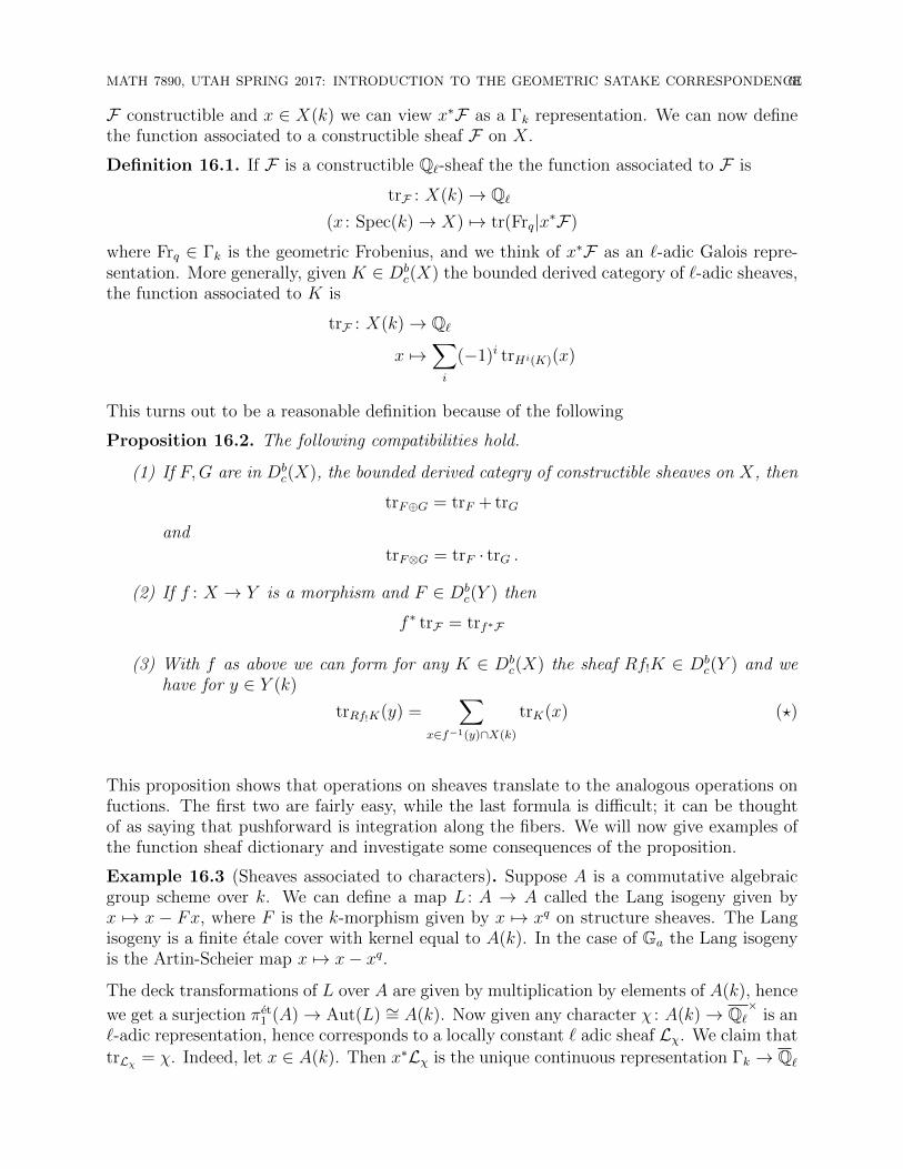
MATH 7890, UTAH SPRING 2017: INTRODUCTION TO THE GEOMETRIC SATAKE CORRESPONDENCE61
F constructible and x ∈ X(k) we can view x∗F as a Γk representation. We can now definethe function associated to a constructible sheaf F on X.
Definition 16.1. If F is a constructible Q`-sheaf the the function associated to F is
trF : X(k)→ Q`
(x : Spec(k)→ X) 7→ tr(Frq|x∗F)
where Frq ∈ Γk is the geometric Frobenius, and we think of x∗F as an `-adic Galois repre-sentation. More generally, given K ∈ Db
c(X) the bounded derived category of `-adic sheaves,the function associated to K is
trF : X(k)→ Q`
x 7→∑i
(−1)i trHi(K)(x)
This turns out to be a reasonable definition because of the following
Proposition 16.2. The following compatibilities hold.
(1) If F,G are in Dbc(X), the bounded derived categry of constructible sheaves on X, then
trF⊕G = trF + trG
and
trF⊗G = trF · trG .
(2) If f : X → Y is a morphism and F ∈ Dbc(Y ) then
f ∗ trF = trf∗F
(3) With f as above we can form for any K ∈ Dbc(X) the sheaf Rf!K ∈ Db
c(Y ) and wehave for y ∈ Y (k)
trRf!K(y) =∑
x∈f−1(y)∩X(k)
trK(x) (?)
This proposition shows that operations on sheaves translate to the analogous operations onfuctions. The first two are fairly easy, while the last formula is difficult; it can be thoughtof as saying that pushforward is integration along the fibers. We will now give examples ofthe function sheaf dictionary and investigate some consequences of the proposition.
Example 16.3 (Sheaves associated to characters). Suppose A is a commutative algebraicgroup scheme over k. We can define a map L : A → A called the Lang isogeny given byx 7→ x − Fx, where F is the k-morphism given by x 7→ xq on structure sheaves. The Langisogeny is a finite etale cover with kernel equal to A(k). In the case of Ga the Lang isogenyis the Artin-Scheier map x 7→ x− xq.
The deck transformations of L over A are given by multiplication by elements of A(k), hence
we get a surjection πet1 (A)→ Aut(L) ∼= A(k). Now given any character χ : A(k)→ Q`
×is an
`-adic representation, hence corresponds to a locally constant ` adic sheaf Lχ. We claim that
trLχ = χ. Indeed, let x ∈ A(k). Then x∗Lχ is the unique continuous representation Γk → Q`
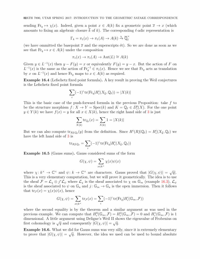
62MATH 7890, UTAH SPRING 2017: INTRODUCTION TO THE GEOMETRIC SATAKE CORRESPONDENCE
sending Frq 7→ χ(x). Indeed, given a point x ∈ A(k) fix a geometric point x → x (which
amounts to fixing an algebraic closure k of k). The corresponding `-adic representation is
Γk = π1(x)→ π1(A)→ A(k)χ−→ Q×`
(we have ommitted the basepoint x and the superscripts et). So we are done as soon as wesee that Frq 7→ x ∈ A(k) under the composition
π1(x)→ π1(A)→ Aut(L) ∼= A(k)
Given y ∈ L−1(x) then y − F (y) = x or equivalently F (y) = y − x. But the action of F onL−1(x) is the same as the action of Fr−1
q ∈ π1(x). Hence we see that Frq acts as translation
by x on L−1(x) and hence Frq maps to x ∈ A(k) as required.
Example 16.4 (Lefschetz fixed point formula). A key result in proving the Weil conjecturesis the Lefschetz fixed point formula∑
i
(−1)i tr(Frq|H ic(Xk,Q`)) = |X(k)|
This is the basic case of the push-forward formula in the previous Proposition: take f tobe the structure morphism f : X → Y = Spec(k) and K = Q` ∈ Db
c(X). For the one pointy ∈ Y (k) we have f(x) = y for all x ∈ X(k), hence the right hand side of 3 is just∑
X(k)
trQ`(x) =∑X(k)
1 = |X(k)|
But we can also compute trRf!Q`(y) from the definition. Since H i(Rf!Q`) = H ic(Xk,Q`) we
have the left hand side of 3 is
trRf!Q` =∑i
(−1)i tr(Frq|H ic(Xk,Q`))
Example 16.5 (Gauss sums). Gauss considered sums of the form
G(χ, ψ) =∑x∈k×
χ(x)ψ(x)
where χ : k× → C× and ψ : k → C× are characters. Gauss proved that |G(χ, ψ)| =√q|.
This is a very elementary computation, but we will prove it geometrically. The idea is to usethe sheaf F = Lχ ⊗ j∗Lψ where Lχ is the sheaf associated to χ on Gm (example 16.3), Lψis the sheaf associated to ψ on Ga and j : Gm → Ga is the open immersion. Then it followsthat trF(x) = χ(x)ψ(x), hence
G(χ, ψ) =∑x∈k×
trF(x) =∑i
(−1)i tr(Frq|H ic(Gm,F))
where the second equality is by the theorem and a similar argument as was used in theprevious example. We can compute that H0
c (Gm,F) = H2c (Gm,F) = 0 and H1
c (Gm,F) is 1dimensional. A little argument using Deligne’s Weil II shows the eigenvalue of Frobenius onfirst cohomology is
√q and consequently |G(χ, ψ)| = √q.
Example 16.6. What we did for Gauss sums was very silly, since it is extremely elementaryto prove that |G(χ, ψ)| =
√q. However, the idea we used can be used to bound absolute
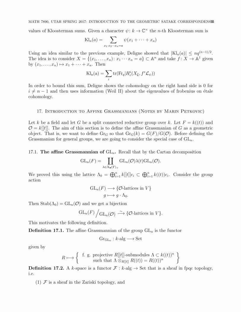
MATH 7890, UTAH SPRING 2017: INTRODUCTION TO THE GEOMETRIC SATAKE CORRESPONDENCE63
values of Kloosterman sums. Given a character ψ : k → C× the n-th Kloosterman sum is
Kln(a) =∑
x1·x2···xn=a
ψ(x1 + · · ·+ xn)
Using an idea similar to the previous example, Deligne showed that |Kln(a)| ≤ nq(n−1)/2.The idea is to consider X = {(x1, . . . , xn) : x1 · · ·xn = a} ⊂ An and take f : X → A1 givenby (x1, . . . , xn) 7→ x1 + · · ·+ xn. Then
Kln(a) =∑i
tr(Frq|H ic(Xk, f
∗Lψ))
In order to bound this sum, Deligne shows the cohomology on the right hand side is 0 fori 6= n − 1 and then uses information (Weil II) about the eigenvalues of frobenius on etalecohomology.
17. Introduction to Affine Grassmanians (Notes by Marin Petkovic)
Let k be a field and let G be a split connected reductive group over k. Let F = k((t)) andO = k[[t]]. The aim of this section is to define the affine Grassmanian of G as a geometricobject. That is, we want to define GrG so that GrG(k) = G(F )/G(O). Before defining theGrassmanian for general groups, we are going to consider the special case of GLn.
17.1. The affine Grassmannian of GLn. Recall that by the Cartan decomposition
GLn(F ) =∐
λ∈X•(T )+
GLn(O)λ(t)GLn(O).
We proved this using the lattice Λ0 =⊕n
i=1 k[[t]]ei ⊂⊕n
i=1 k((t))ei. Consider the groupaction
GLn(F ) −→ {O-lattices in V }g 7−→ g · Λ0.
Then Stab(Λ0) = GLn(O) and we get a bijection
GLn(F )/
GLn(O)∼−→ {O-lattices in V }.
This motivates the following definition.
Definition 17.1. The affine Grassmannian of the group GLn is the functor
GrGLn : k-alg −→ Set
given by
R 7−→{
f. g. projective R[[t]]-submodules Λ ⊂ k((t))n
such that Λ⊗R[[t]] R((t)) = R((t))n
}Definition 17.2. A k-space is a functor F : k-alg → Set that is a sheaf in fpqc topology,i.e.
(1) F is a sheaf in the Zariski topology, and
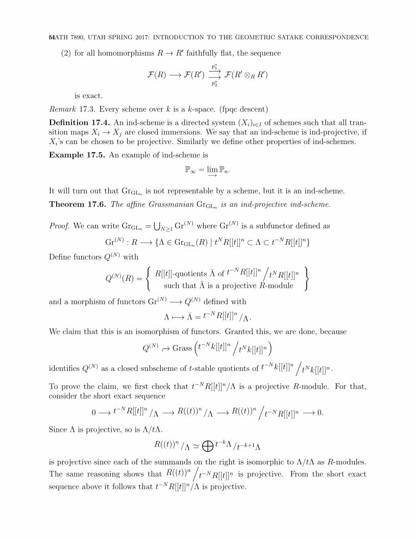
64MATH 7890, UTAH SPRING 2017: INTRODUCTION TO THE GEOMETRIC SATAKE CORRESPONDENCE
(2) for all homomorphisms R→ R′ faithfully flat, the sequence
F(R) −→ F(R′)p∗1−→−→p∗2
F(R′ ⊗R R′)
is exact.
Remark 17.3. Every scheme over k is a k-space. (fpqc descent)
Definition 17.4. An ind-scheme is a directed system (Xi)i∈I of schemes such that all tran-sition maps Xi → Xj are closed immersions. We say that an ind-scheme is ind-projective, ifXi’s can be chosen to be projective. Similarly we define other properties of ind-schemes.
Example 17.5. An example of ind-scheme is
P∞ = lim−→
Pn.
It will turn out that GrGLn is not representable by a scheme, but it is an ind-scheme.
Theorem 17.6. The affine Grassmanian GrGLn is an ind-projective ind-scheme.
Proof. We can write GrGLn =⋃N≥1 Gr(N) where Gr(N) is a subfunctor defined as
Gr(N) : R −→ {Λ ∈ GrGLn(R) | tNR[[t]]n ⊂ Λ ⊂ t−NR[[t]]n}
Define functors Q(N) with
Q(N)(R) =
{R[[t]]-quotients Λ of t
−NR[[t]]n/tNR[[t]]n
such that Λ is a projective R-module
}and a morphism of functors Gr(N) −→ Q(N) defined with
Λ 7−→ Λ = t−NR[[t]]n /Λ .
We claim that this is an isomorphism of functors. Granted this, we are done, because
Q(N) ↪−→ Grass(t−Nk[[t]]n
/tNk[[t]]n
)identifies Q(N) as a closed subscheme of t-stable quotients of t
−Nk[[t]]n/tNk[[t]]n .
To prove the claim, we first check that t−NR[[t]]n/Λ is a projective R-module. For that,consider the short exact sequence
0 −→ t−NR[[t]]n /Λ −→ R((t))n /Λ −→ R((t))n/t−NR[[t]]n −→ 0.
Since Λ is projective, so is Λ/tΛ.
R((t))n /Λ '⊕
t−kΛ /t−k+1Λ
is projective since each of the summands on the right is isomorphic to Λ/tΛ as R-modules.
The same reasoning shows that R((t))n/t−NR[[t]]n is projective. From the short exact
sequence above it follows that t−NR[[t]]n/Λ is projective.
MATH 7890, UTAH SPRING 2017: INTRODUCTION TO THE GEOMETRIC SATAKE CORRESPONDENCE65
To show bijectivity, let Q ∈ Q(N)(R). As we have seen, Q(N) is of finite type over k, so forall k-algebras R we have
Q(N)(R) = colimf.g. Ri⊂R
Q(N)(Ri).
We may therefore assume R is finitely-generated over k.
We have
t−NR[[t]]n � t−NR[[t]]n/tNR[[t]]n � Q,
so let ΛQ be the kernel of the composition above. We need to show that ΛQ ∈ Gr(N)(R).Since tNR[[t]]n ⊂ ΛQ, we know that Λ ⊗ R((t)) = R((t))n, so it remains to show thatΛQ is finitely generated projective R[[t]]-module. Since R is finitely generated over k, it isNoetherian. In particular R[t] −→ R[[t]] is flat.
Since
t−NR[t]n � t−NR[t]n/tNR[t]n ∼−− t−NR[[t]]n
/tNR[[t]]n � Q
we can define ΛQ,fin = ker(t−NR[t]n � Q). Since R[t] −→ R[[t]] is flat, ΛQ,fin⊗R[t]R[[t]] = ΛQ.Hence it suffices to show that ΛQ,fin is finitely generated projective R[t]-module. It is clearlyfinitely generated, since it is contained in t−NR[t]n. To show ΛQ,fin is projective, we will showit is flat over R[t].
For this, notice that ∀p ∈ Spec(R), ΛQ,fin⊗R[t] κ(p)[t] is flat (and therefore free) over κ(p)[t].Indeed, since Q is R-flat, we have
ΛQ,fin ⊗R[t] κ(p)[t] = ker(t−Nκ(p)[t]n −→ Q⊗R κ(p)
).
Since t−Nκ(p)[t]n is torsion free, so is ΛQ,fin ⊗R[t] κ(p)[t], and hence it is flat. Now apply thefollowing lemma on Rp −→ R[t]q and M = ΛQ,fin ⊗R[t]q, for all primes q of R[t].
�
Lemma 17.7. Let R −→ S be a local homomorphism of Noetherian local rings, m ⊂ Rmaximal ideal and M a finite S-module. If M is flat over R and M/mM is free over S/mS,then M is free over S and S is flat over R.
Proof. Stacks Tag 00MH �
17.2. Affine Grassmanian for general groups. Let DR = Spec(R[[t]]) (family of disksparametrized by R) and D∗R = Spec(R((t))) (family of punctured disks parametrized by R).
We can identify
GrGLn(R) =
{(E , β)
∣∣∣ E is a vector bundle of rank n on DRand β : E
∣∣D∗R
∼−→ the trivial bundle on D∗R
}/' .
Proposition 17.8. Let G be a linear group over k and S quasi-compact scheme. Thefollowing categories are equivalent:
66MATH 7890, UTAH SPRING 2017: INTRODUCTION TO THE GEOMETRIC SATAKE CORRESPONDENCE
(1) fpqc sheafs P on Aff/S which are right G-torsors, i.e. P has a right G action suchthat
P ×G −→ P ×S P(s, g) 7−→ (s, sg)
is an isomorphism, and for which there exists an fpqc cover S ′ −→ S such thatP(S ′) 6= ∅.
(2) scheme maps π : E −→ S with a right G-action on E equivariant for π such thatthere exists a faithfully flat cover S ′ −→ S such that E ×S S ′ ' G× S ′ as G-torsors.
(3) faithfully flat maps E −→ S with a right G-action such that E ×S E ' G × E asG-torsors.
(4) If G is smooth, as in (2) but require S ′ −→ S etale.
Remark 17.9. All the non-obvious implications follow from faithfully flat descent theory.
Definition 17.10. A G-bundle is an object in any of the four equivalent categories above(we will use (4)). The trivial G-bundle over S is E0 = G ×k S with G acting on itself byright multiplication.
Definition 17.11. The affine Grassmannian of G is the functor
GrG : k-alg −→ Set
given by
R 7−→
{(E , β)
∣∣∣ E is a G-bundle on DR and
β : E∣∣D∗R
∼−→ E0 is an isomorphism of G-bundles
}/' .
Relation to previous definition for GLn
For any S there is an equivalence:
{GLn-bundles over S} −→ {rank n vector bundles over S}
(E → S) 7−→ EGLn× An
where E GLn× An = GLn∖E × An
with the action given by g.(s, v) = (sg−1, gv). Its quasi-inverse is given by
V 7−→
(T 7→ IsomT (OnT ,V)
GLn
),
for all V rank n vector bundle over S.
Theorem 17.12. For any affine G/k the presheaf GrG is representable by an ind-scheme ofind-finite type. If G is reductive, then GrG is moreover ind-projective.
MATH 7890, UTAH SPRING 2017: INTRODUCTION TO THE GEOMETRIC SATAKE CORRESPONDENCE67
Strategy of proof. Choose an embedding G −→ GLn such that GLn/G is quasi-affine. In thiscase, one can show that the map
GrG −→ GrGLn
E 7−→ EG×GLn
is a locally closed embedding.
When G is reductive, GLn/G is affine and the map above is a closed embedding. �
For general homomorphisms H −→ G, the map GrH −→ GrG may be very strange.
Example 17.13. Let B < G be a Borel subgroup. If G is reductive, the Iwasawa decompo-sition says G(k((t))) = B(k((t))) ·G(k[[t]]), so GrB −→ GrG is a bijection on k-points. Thismap is far from being an isomorphism.
17.3. Another description of GrG. We would like a description of GrG that is closer toour intuitive understanding of it as the “quotient” G(k((t)))/G(k[[t]]). Define the loop groupof G to be
LG : k-alg −→ Grp
R 7−→ G(R((t)))
and the positive loop group
L+G : k-alg −→ Grp
R 7−→ G(R[[t]])
Lemma 17.14. L+G is a scheme over k and LG is an ind-scheme over k.
Proof for GLn. Notice that
L+G(R) = GLn(R[[t]]) =
(∑m≥0
bi,j,mtm
)i,j
∣∣∣ bi,j,m ∈ R, det ∈ R×
can be embedded into the affine scheme R[{xi,j,m}, det], and
LG(R) =⋃r≥0
{matrices with all entries having poles of order at most r}
and all the objects on the right are schemes. �
Now consider the presheaf
LG /L+G : R 7−→ LG(R)/
L+G(R) .
Let[LG /L+G
]be the sheafication for the fpqc (or fppf, or etale) topology. As we will see,
when G is smooth the choice of topology does not matter.
Proposition 17.15. For any smooth linear algebraic group G/k, GrG is naturally isomorphicto[LG /L+G
].
68MATH 7890, UTAH SPRING 2017: INTRODUCTION TO THE GEOMETRIC SATAKE CORRESPONDENCE
Before the proof, we apply the Proposition to an example:
Example 17.16. Consider LGm/L+Gm. Let f =
∑ant
n ∈ LGm(R) = R((t))×. Then thereexists n0 such that an0 ∈ R× and an is nilpotent for all n < n0 (eg. if R = k[ε]/ε2, thenεt−1 + 1 ∈ R((t))× since (εt−1 + 1)(−εt−1 + 1) = 1). Write f(t) = an0t
n0g(t) where thenegative powers of t in g(t) have nilpotent coefficients. Then g(t) can be factored uniquelyas a product of a polynomial with degrees ≤ 0 and nilpotent coefficients with a polynomialin 1 + tR[[t]]. Hence we obtain a decomposition
LGm = Gm × Z× (R 7→ 1 + tR[[t]])× (some highly non-reduced ind-scheme).
Under this composition L+Gm = Gm × A∞, so
LGm/
L+Gm' Z× (some highly non-reduced ind-scheme).
In particular, GrGm is not reduced and π0GrGm = Z.
Proof of proposition. There is an isomorphism
LG(R)∼−→
(E , β, ε)
∣∣∣∣∣E is a G-bundle on DR
β : E∣∣D∗R
∼−→ E0
ε : E ∼−→ E0
/'
g 7−→ (E0, g, id)
where we interpret g as an automorphism of E0 over D∗R. Let LG −→ GrG be the obviousmorphism that forgets ε. Since L+G(R) = Aut(E0/DR), this map factors and we obtainLG /L+G −→ GrG. Since GrG is a sheaf (for fpqc topology and hence for etale topology)this induces a map of sheaves [
LG /L+G]−→ GrG.
It is easy to see that this is injective, so it remains to prove surjectivity. This follows fromthe following lemma. �
Lemma 17.17. Any G-bundle E on DR can be trivialized etale locally on R, i.e. there existsetale cover R −→ R′ such that E ⊗R[[t]] R
′[[t]] is isomorphic to the trivial bundle on DR′.
Proof. We claim that E is trivial over DR iff E ×R[[t]] R is trivial over R. To see this, recall
that E∣∣S′
is trivial iff E(S ′) 6= ∅. Since E is smooth, the maps E(R[t]/tn+1) −→ E(R[t]/tn)are all surjections. Since E is affine, E(R[[t]]) = lim
←E(R[t]/tn). Thus, if (E ×R[[t]] R)(R) 6= 0,
then E(R[[t]]) 6= 0, which is equivalent to E being trivial over DR.
Having established the claim, the lemma follows since E ⊗R[[t]] R is a G-bundle over R, so itcan be trivialized etale locally on R. �
Let G be connected reductive group and T ⊂ B ⊂ G a maximal torus and Borel subgroup.Let λ ∈ X•(T )+. Then λ(t) ∈ GrG(k). The positive loop group L+G acts on GrG =[LG /L+G
]by left multiplication.
Definition 17.18. Let GrG,λ be the L+G-orbit of λ(t), regarded as a locally closed reducedsubscheme of GrG. Define GrG,≤λ = GrG,λ ↪→ GrG.
MATH 7890, UTAH SPRING 2017: INTRODUCTION TO THE GEOMETRIC SATAKE CORRESPONDENCE69
Now we can answer the motivating question from classical Satake:
There is a complex of sheaves ICλ called the intersection complex on GrG,≤λ such that underthe sheaf-function dictionary:
HG(k[[t]])∼−→ R(G∨)
tr(ICλ) 7−→ ch(V (λ)).
The intersection complex is the basic example of a perverse sheaf; we turn to this subject inthe next part of the course.
18. Review of homological algebra (Allechar Serrano Lopez)
1. Let C be an additive category. Set C(C) = category of complexes
· · · → Xn → Xn+1 → · · ·
in C and K(C) = category of complexes modulo chain homotopy equivalence, i.e.
obK(C) = obC(C)HomK(C)(X, Y ) = HomC(C)(X, Y )/ ∼
where ∼ is given by f ∼ g if there exists a chain homotopy between them.
Recall
· · · Xn−1 Xn Xn+1 · · ·
· · · Y n−1 Y n Y n+1 · · ·s s
a chain homotopy between maps f, g : X → Y is a collection sn : Xn → Y n−1 suchthat f − g = ds+ sd.
We will write C?(C) and K?(C) to denote the analogous categories of complexesbounded from below (? = +), from above (? = −), or from both directions (? = b).
Example 18.1. If C is an abelian category. Any complexX ∈ C(C) has (co)homologyobjects in C, namely
Hn(X) =ker(dnX)
image(dn−1X )
∈ C
Maps in C(C) induce maps on homology, and homotopic maps induce the same mapon Hn.
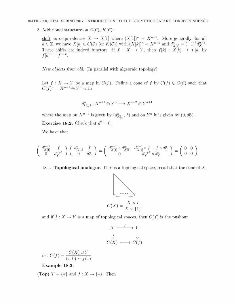
70MATH 7890, UTAH SPRING 2017: INTRODUCTION TO THE GEOMETRIC SATAKE CORRESPONDENCE
2. Additional structure on C(C), K(C):
shift autoequivalences X → X[1] where (X[1])n = Xn+1. More generally, for allk ∈ Z, we have X[k] ∈ C(C) (or K(C)) with (X[k])n = Xn+k and dnX[k] = (−1)kdn+k
X .
These shifts are indeed functors: if f : X → Y , then f [k] : X[k] → Y [k] byf [k]n = fn+k.
New objects from old: (In parallel with algebraic topology)
Let f : X → Y be a map in C(C). Define a cone of f by C(f) ∈ C(C) such thatC(f)n = Xn+1 ⊕ Y n with
dnC(f) : Xn+1 ⊕ Y n −→ Xn+2 ⊕ Y n+1
where the map on Xn+1 is given by (dnX[1], f) and on Y n it is given by (0, dnY ).
Exercise 18.2. Check that d2 = 0.
We have that
(dn+1X[1] f
0 dn+1Y
)(dnX[1] f
0 dnY
)=
(dn+1X[1] ◦ dnX[1] dn+1
X[1] ◦ f + f ◦ dnY0 dn+1
Y ◦ dnY
)=
(0 00 0
)
18.1. Topological analogue. If X is a topological space, recall that the cone of X,
C(X) =X × IX × {1}
and if f : X → Y is a map of topological spaces, then C(f) is the pushout
X Y
C(X) C(f)
f
i
i.e. C(f) =C(X) ∪ Y
(x, 0) ∼ f(x)
Example 18.3.
(Top) Y = {∗} and f : X → {∗}. Then
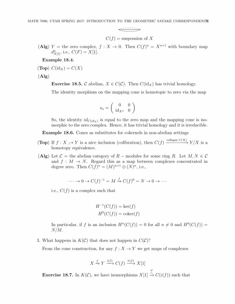
MATH 7890, UTAH SPRING 2017: INTRODUCTION TO THE GEOMETRIC SATAKE CORRESPONDENCE71
C(f) = suspension of X
(Alg) Y = the zero complex, f : X → 0. Then C(f)n = Xn+1 with boundary mapdnX[1], i.e., C(F ) = X[1].
Example 18.4.
(Top) C(idX) = C(X)
(Alg)
Exercise 18.5. C abelian, X ∈ C(C). Then C(idX) has trivial homology.
The identity morphism on the mapping cone is homotopic to zero via the map
sn =
(0 0
idXn 0
)So, the identity idC(idX) is equal to the zero map and the mapping cone is iso-morphic to the zero complex. Hence, it has trivial homology and it is irreducible.
Example 18.6. Cones as substitutes for cokernels in non-abelian settings
(Top) If f : X ↪→ Y is a nice inclusion (cofibration), then C(f)collapse C(X)−−−−−−−−→ Y/X is a
homotopy equivalence.
(Alg) Let C = the abelian category of R − modules for some ring R. Let M,N ∈ Cand f : M → N . Regard this as a map between complexes concentrated indegree zero. Then C(f)n = (M)n+1 ⊕ (N)n, i.e.,
· · · → 0→ C(f)−1 = Mf−→ C(f)0 = N → 0→ · · ·
i.e., C(f) is a complex such that
H−1(C(f)) = ker(f)
H0(C(f)) = coker(f)
In particular, if f is an inclusion Hn(C(f)) = 0 for all n 6= 0 and H0(C(f)) =N/M .
3. What happens in K(C) that does not happen in C(C)?
From the cone construction, for any f : X → Y we get maps of complexes
Xf−→ Y
i(f)−−→ C(f)π(f)−−→ X[1]
Exercise 18.7. In K(C), we have isomorphisms X[1]ψ∼−→ C(i(f)) such that
72MATH 7890, UTAH SPRING 2017: INTRODUCTION TO THE GEOMETRIC SATAKE CORRESPONDENCE
Y C(f) X[1] Y [1]
Y C(f) C(i(f)) Y [1]
i(f) π(f)
∼ψ
−f [1]
i(f) i(i(f)) π(i(f))
commutes in K(C).
We want to show that the rotated triangle
Yi(f)−−→ C(f)
π(f)−−→ X[1]−f [1]−−−→ Y [1]
is isomorphic in K(C) to the standard triangle for i(f)
Yi(f)−−→ C(f)
i(i(f))−−−→ C(i(f))π(i(f))−−−−→ Y [1]
Define φ = (φn) : X[1] → C(i(f)) by setting φ = (−f, idX , 0) and define ψ :C(i(f)) → X[1] by setting ψ : (0, idX , 0). These gives morphisms of triangles sincewe have π(i(f)) ◦ φ = −f [1] and φ ◦ π(f) ∼ i(i(f)). Similarly, ψ is a morphism oftriangles since π(f) = ψ ◦ (i(i(f))) and −f [1] ◦ ψ ∼ π(i(f)). Now, this morphismsare isomorphisms since ψ ◦ φ = idX[1] and φ ◦ ψ ∼ idC(i(f)).
Definition 18.8. A triangle, 4, in K(C) is any sequence of maps
X → Y → Z → X[1]
A distinguished triangle is a triangle that is isomorphic to one of the form
Xf−→ Y
i(f)−−→ C(f)π(f)−−→ X[1]
for some map f .
Theorem 18.9. (Verdier) For an additive category C, K(C) equipped with its shiftautoequivalence [1] and its collection of distinguished triangles is a triangulated cate-gory.
Here’s what this means:
Definition 18.10. A triangulated category is an additive abelian category D withautoequivalence [1] : D → D and a designated collection of “distinguished triangles”inside the collection of all triangles, satisfying
(TR1) – For all X ∈ D, XidX−−→ X → 0→ X[1] is a distinguished triangle
– any triangle isomorphic to a distinguished triangle is itself distinguished
– any map f : X → Y can be completed to a distinguished triangle, i.e.,
there exist Z and maps such that Xf−→ Y → Z → X[1] is a distinguished
triangle; such a Z is called a cone of f .
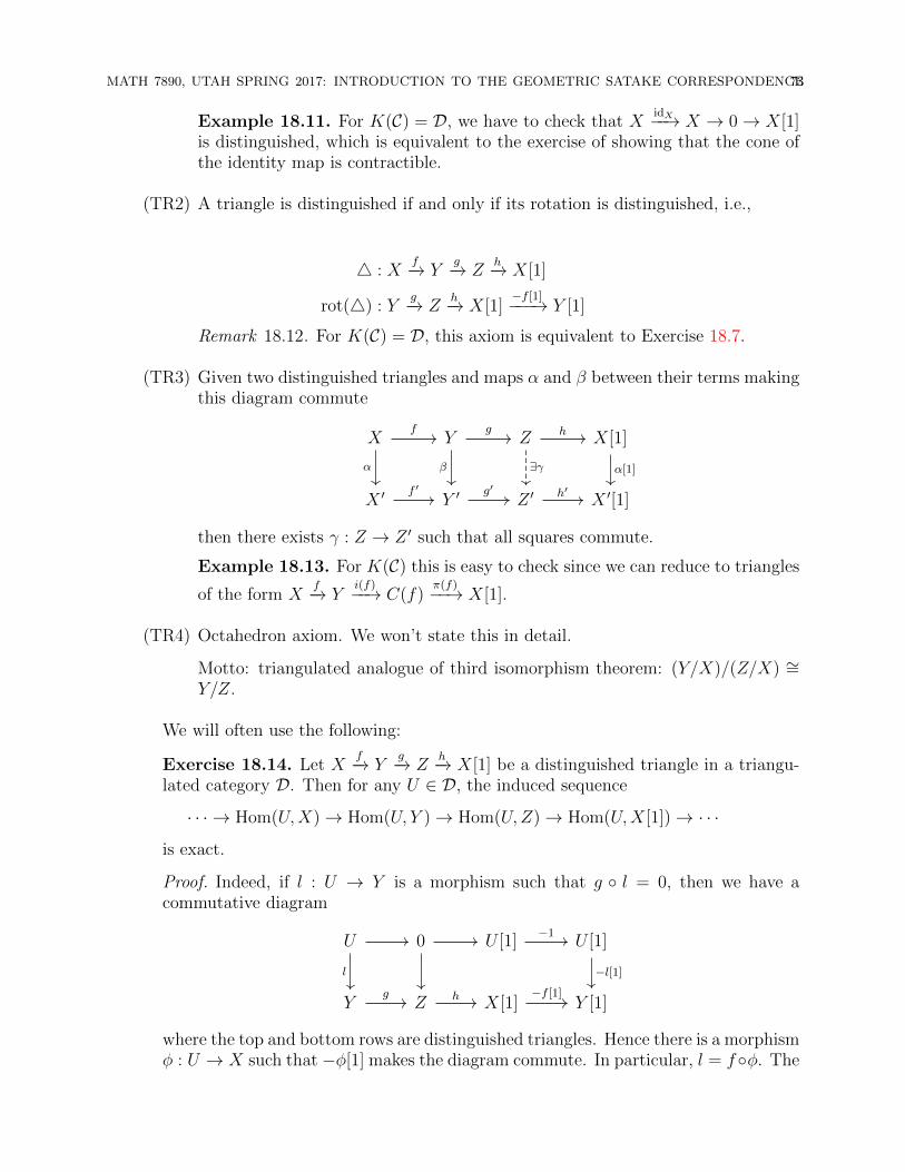
MATH 7890, UTAH SPRING 2017: INTRODUCTION TO THE GEOMETRIC SATAKE CORRESPONDENCE73
Example 18.11. For K(C) = D, we have to check that XidX−−→ X → 0→ X[1]
is distinguished, which is equivalent to the exercise of showing that the cone ofthe identity map is contractible.
(TR2) A triangle is distinguished if and only if its rotation is distinguished, i.e.,
4 : Xf−→ Y
g−→ Zh−→ X[1]
rot(4) : Yg−→ Z
h−→ X[1]−f [1]−−−→ Y [1]
Remark 18.12. For K(C) = D, this axiom is equivalent to Exercise 18.7.
(TR3) Given two distinguished triangles and maps α and β between their terms makingthis diagram commute
X Y Z X[1]
X ′ Y ′ Z ′ X ′[1]
f
α
g
β
h
∃γ α[1]
f ′ g′ h′
then there exists γ : Z → Z ′ such that all squares commute.
Example 18.13. For K(C) this is easy to check since we can reduce to triangles
of the form Xf−→ Y
i(f)−−→ C(f)π(f)−−→ X[1].
(TR4) Octahedron axiom. We won’t state this in detail.
Motto: triangulated analogue of third isomorphism theorem: (Y/X)/(Z/X) ∼=Y/Z.
We will often use the following:
Exercise 18.14. Let Xf−→ Y
g−→ Zh−→ X[1] be a distinguished triangle in a triangu-
lated category D. Then for any U ∈ D, the induced sequence
· · · → Hom(U,X)→ Hom(U, Y )→ Hom(U,Z)→ Hom(U,X[1])→ · · ·
is exact.
Proof. Indeed, if l : U → Y is a morphism such that g ◦ l = 0, then we have acommutative diagram
U 0 U [1] U [1]
Y Z X[1] Y [1]
l
−1
−l[1]
g h −f [1]
where the top and bottom rows are distinguished triangles. Hence there is a morphismφ : U → X such that −φ[1] makes the diagram commute. In particular, l = f◦φ. The
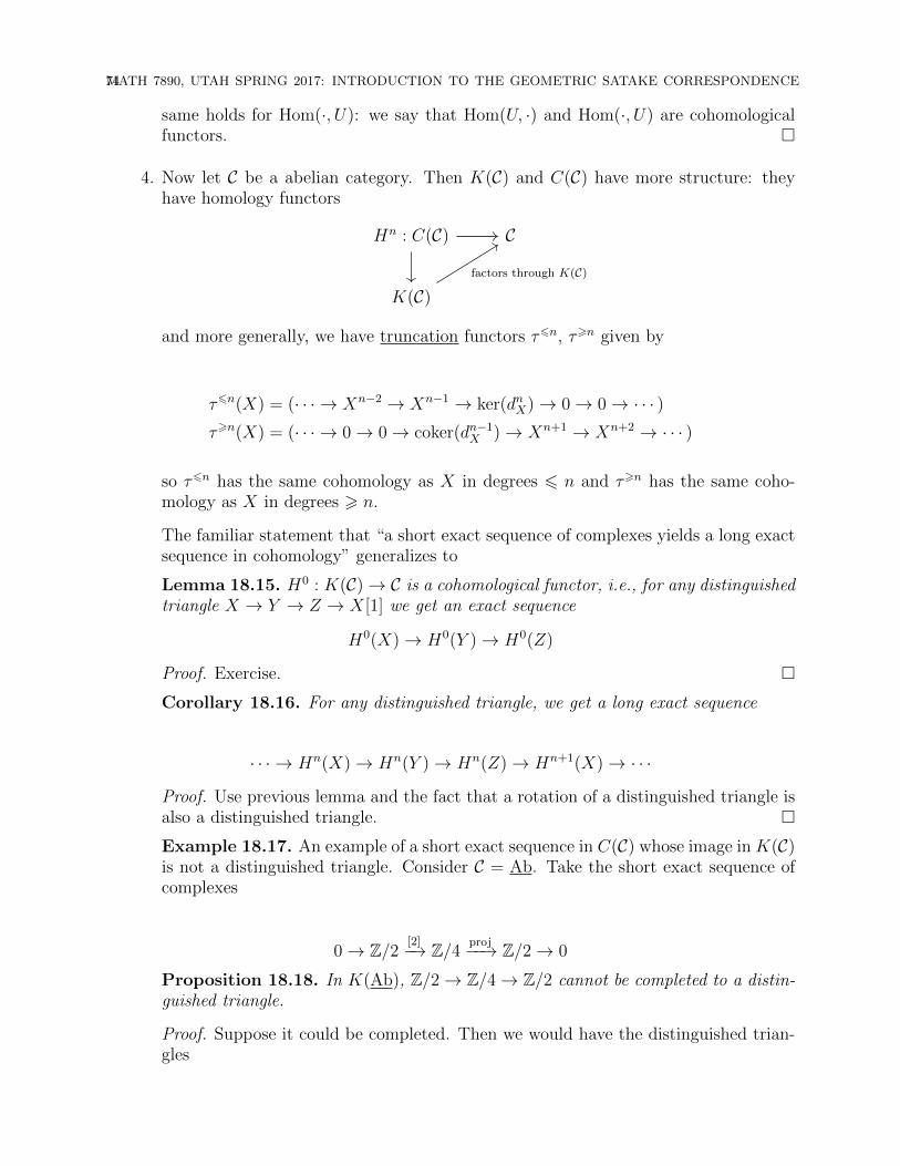
74MATH 7890, UTAH SPRING 2017: INTRODUCTION TO THE GEOMETRIC SATAKE CORRESPONDENCE
same holds for Hom(·, U): we say that Hom(U, ·) and Hom(·, U) are cohomologicalfunctors. �
4. Now let C be a abelian category. Then K(C) and C(C) have more structure: theyhave homology functors
Hn : C(C) C
K(C)factors through K(C)
and more generally, we have truncation functors τ6n, τ>n given by
τ6n(X) = (· · · → Xn−2 → Xn−1 → ker(dnX)→ 0→ 0→ · · · )τ>n(X) = (· · · → 0→ 0→ coker(dn−1
X )→ Xn+1 → Xn+2 → · · · )
so τ6n has the same cohomology as X in degrees 6 n and τ>n has the same coho-mology as X in degrees > n.
The familiar statement that “a short exact sequence of complexes yields a long exactsequence in cohomology” generalizes to
Lemma 18.15. H0 : K(C)→ C is a cohomological functor, i.e., for any distinguishedtriangle X → Y → Z → X[1] we get an exact sequence
H0(X)→ H0(Y )→ H0(Z)
Proof. Exercise. �
Corollary 18.16. For any distinguished triangle, we get a long exact sequence
· · · → Hn(X)→ Hn(Y )→ Hn(Z)→ Hn+1(X)→ · · ·
Proof. Use previous lemma and the fact that a rotation of a distinguished triangle isalso a distinguished triangle. �
Example 18.17. An example of a short exact sequence in C(C) whose image in K(C)is not a distinguished triangle. Consider C = Ab. Take the short exact sequence ofcomplexes
0→ Z/2 [2]−→ Z/4 proj−−→ Z/2→ 0
Proposition 18.18. In K(Ab), Z/2→ Z/4→ Z/2 cannot be completed to a distin-guished triangle.
Proof. Suppose it could be completed. Then we would have the distinguished trian-gles
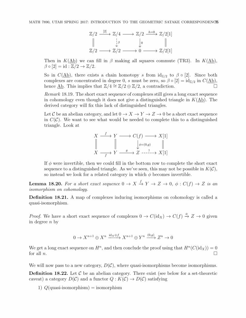
MATH 7890, UTAH SPRING 2017: INTRODUCTION TO THE GEOMETRIC SATAKE CORRESPONDENCE75
Z/2 Z/4 Z/2 Z/2[1]
Z/2 Z/2 0 Z/2[1]
[2]
β
h=0
0
Then in K(Ab) we can fill in β making all squares commute (TR3). In K(Ab),β ◦ [2] = id : Z/2→ Z/2.
So in C(Ab), there exists a chain homotopy s from idZ/2 to β ◦ [2]. Since bothcomplexes are concentrated in degree 0, s must be zero, so β ◦ [2] = idZ/2 in C(Ab),hence Ab. This implies that Z/4 ∼= Z/2⊕ Z/2, a contradiction. �
Remark 18.19. The short exact sequence of complexes still gives a long exact sequencein cohomology even though it does not give a distinguished triangle in K(Ab). Thederived category will fix this lack of distinguished triangles.
Let C be an abelian category, and let 0→ X → Y → Z → 0 be a short exact sequencein C(C). We want to see what would be needed to complete this to a distinguishedtriangle. Look at
X Y C(f) X[1]
X Y Z X[1]
f
φ=(0,g)
f
g ?
If φ were invertible, then we could fill in the bottom row to complete the short exactsequence to a distinguished triangle. As we’ve seen, this may not be possible in K(C),so instead we look for a related category in which φ becomes invertible.
Lemma 18.20. For a short exact sequence 0 → Xf−→ Y → Z → 0, φ : C(f) → Z is an
isomorphism on cohomology.
Definition 18.21. A map of complexes inducing isomorphisms on cohomology is called aquasi-isomorphism.
Proof. We have a short exact sequence of complexes 0 → C(idX) → C(f)φ−→ Z → 0 given
in degree n by
0→ Xn+1 ⊕Xn idX⊕f−−−−→ Xn+1 ⊕ Y n (0,g)−−→ Zn → 0
We get a long exact sequence on Hn, and then conclude the proof using that Hn(C(idX)) = 0for all n. �
We will now pass to a new category, D(C), where quasi-isomorphisms become isomorphisms.
Definition 18.22. Let C be an abelian category. There exist (see below for a set-theoreticcaveat) a category D(C) and a functor Q : K(C)→ D(C) satisfying
1) Q(quasi-isomorphism) = isomorphism
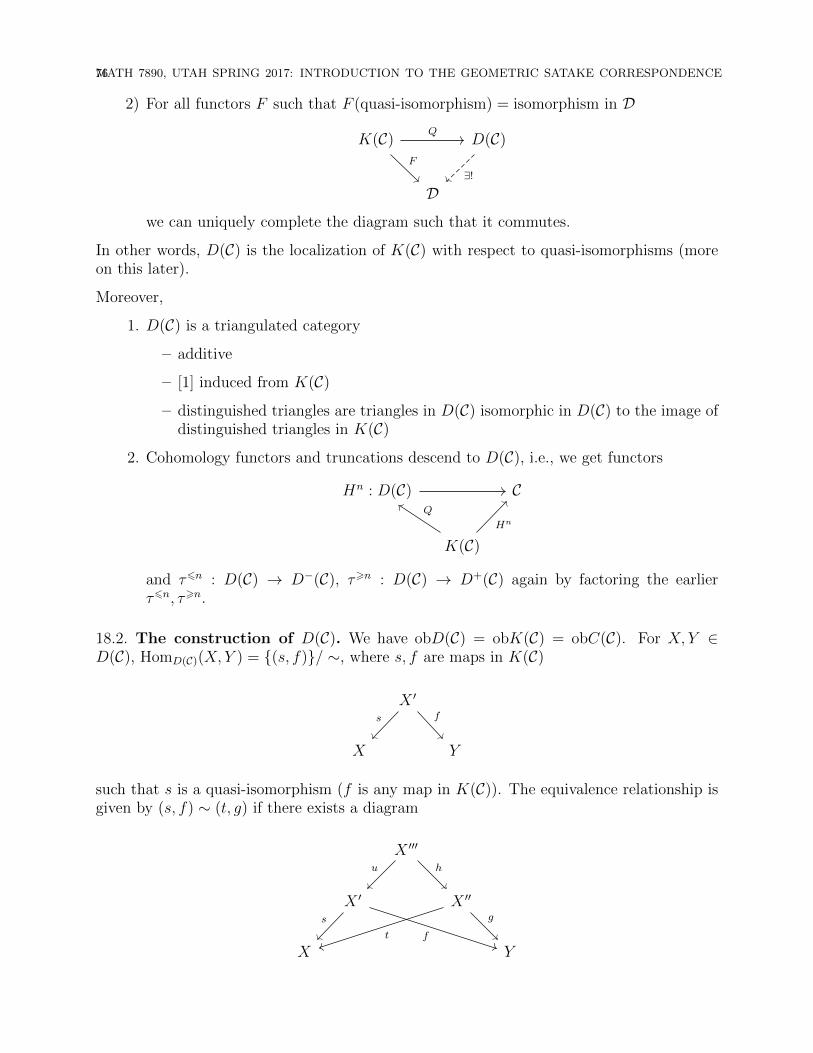
76MATH 7890, UTAH SPRING 2017: INTRODUCTION TO THE GEOMETRIC SATAKE CORRESPONDENCE
2) For all functors F such that F (quasi-isomorphism) = isomorphism in D
K(C) D(C)
D
Q
F
∃!
we can uniquely complete the diagram such that it commutes.
In other words, D(C) is the localization of K(C) with respect to quasi-isomorphisms (moreon this later).
Moreover,
1. D(C) is a triangulated category
– additive
– [1] induced from K(C)
– distinguished triangles are triangles in D(C) isomorphic in D(C) to the image ofdistinguished triangles in K(C)
2. Cohomology functors and truncations descend to D(C), i.e., we get functors
Hn : D(C) C
K(C)
Q
Hn
and τ6n : D(C) → D−(C), τ>n : D(C) → D+(C) again by factoring the earlierτ6n, τ>n.
18.2. The construction of D(C). We have obD(C) = obK(C) = obC(C). For X, Y ∈D(C), HomD(C)(X, Y ) = {(s, f)}/ ∼, where s, f are maps in K(C)
X ′
X Y
s f
such that s is a quasi-isomorphism (f is any map in K(C)). The equivalence relationship isgiven by (s, f) ∼ (t, g) if there exists a diagram
X ′′′
X ′ X ′′
X Y
u h
s
f
g
t
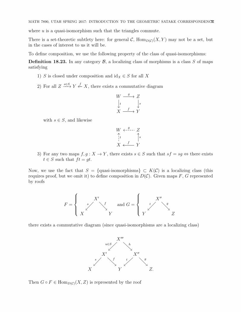
MATH 7890, UTAH SPRING 2017: INTRODUCTION TO THE GEOMETRIC SATAKE CORRESPONDENCE77
where u is a quasi-isomorphism such that the triangles commute.
There is a set-theoretic subtlety here: for general C, HomD(C)(X, Y ) may not be a set, butin the cases of interest to us it will be.
To define composition, we use the following property of the class of quasi-isomorphisms:
Definition 18.23. In any category B, a localizing class of morphisms is a class S of mapssatisfying
1) S is closed under composition and idX ∈ S for all X
2) For all Zs∈S−−→ Y
f←− X, there exists a commutative diagram
W Z
X Y
g
t s
f
with s ∈ S, and likewise
W Z
X Y
g
t s
f
3) For any two maps f, g : X → Y , there exists s ∈ S such that sf = sg ⇔ there existst ∈ S such that ft = gt.
Now, we use the fact that S = {quasi-isomorphisms} ⊂ K(C) is a localizing class (thisrequires proof, but we omit it) to define composition in D(C). Given maps F , G representedby roofs
F =
X ′
X Y
s f and G =
X ′′
Y Z
t g
there exists a commutative diagram (since quasi-isomorphisms are a localizing class)
X ′′′
X ′ X ′′
X Y Z.
u∈S h
s f gt
Then G ◦ F ∈ HomD(C)(X,Z) is represented by the roof
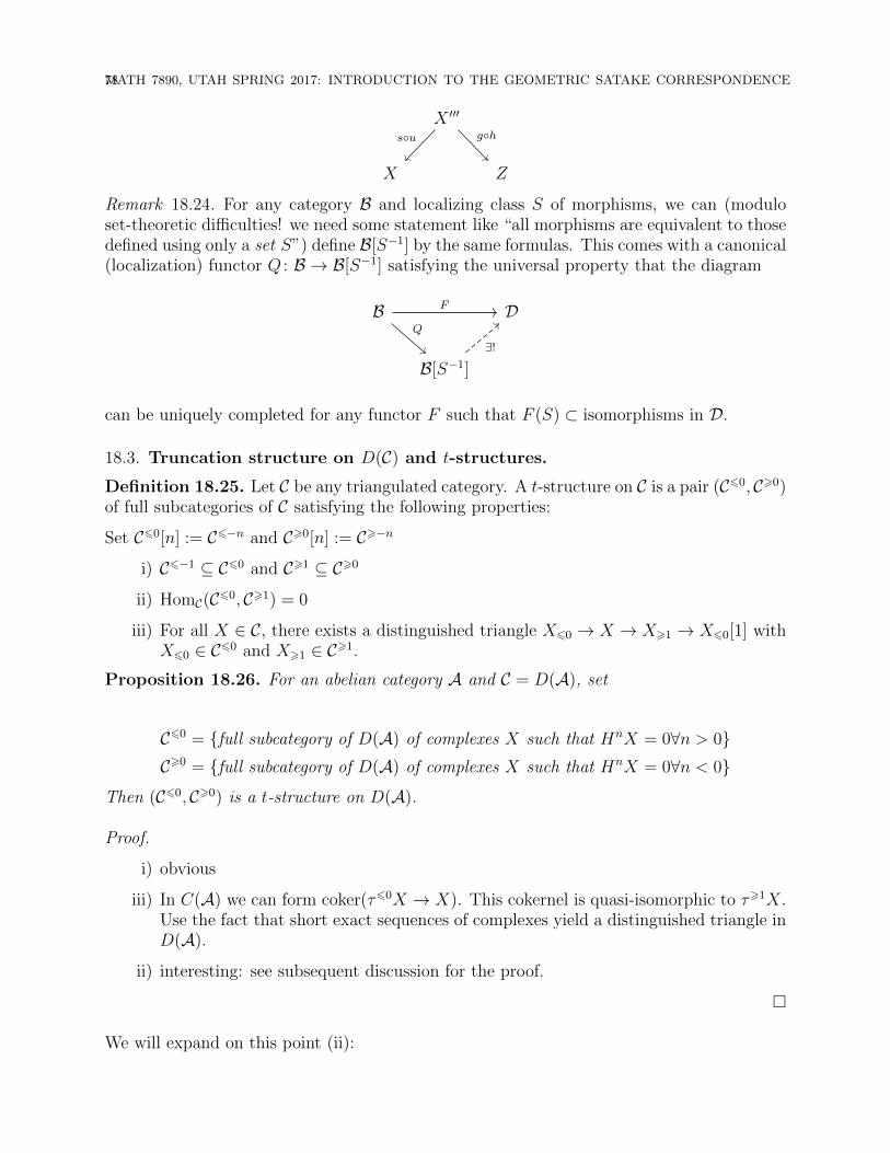
78MATH 7890, UTAH SPRING 2017: INTRODUCTION TO THE GEOMETRIC SATAKE CORRESPONDENCE
X ′′′
X Z
s◦u g◦h
Remark 18.24. For any category B and localizing class S of morphisms, we can (moduloset-theoretic difficulties! we need some statement like “all morphisms are equivalent to thosedefined using only a set S”) define B[S−1] by the same formulas. This comes with a canonical(localization) functor Q : B → B[S−1] satisfying the universal property that the diagram
B D
B[S−1]
F
Q
∃!
can be uniquely completed for any functor F such that F (S) ⊂ isomorphisms in D.
18.3. Truncation structure on D(C) and t-structures.
Definition 18.25. Let C be any triangulated category. A t-structure on C is a pair (C60, C>0)of full subcategories of C satisfying the following properties:
Set C60[n] := C6−n and C>0[n] := C>−n
i) C6−1 ⊆ C60 and C>1 ⊆ C>0
ii) HomC(C60, C>1) = 0
iii) For all X ∈ C, there exists a distinguished triangle X60 → X → X>1 → X60[1] withX60 ∈ C60 and X>1 ∈ C>1.
Proposition 18.26. For an abelian category A and C = D(A), set
C60 = {full subcategory of D(A) of complexes X such that HnX = 0∀n > 0}C>0 = {full subcategory of D(A) of complexes X such that HnX = 0∀n < 0}
Then (C60, C>0) is a t-structure on D(A).
Proof.
i) obvious
iii) In C(A) we can form coker(τ60X → X). This cokernel is quasi-isomorphic to τ>1X.Use the fact that short exact sequences of complexes yield a distinguished triangle inD(A).
ii) interesting: see subsequent discussion for the proof.
�
We will expand on this point (ii):
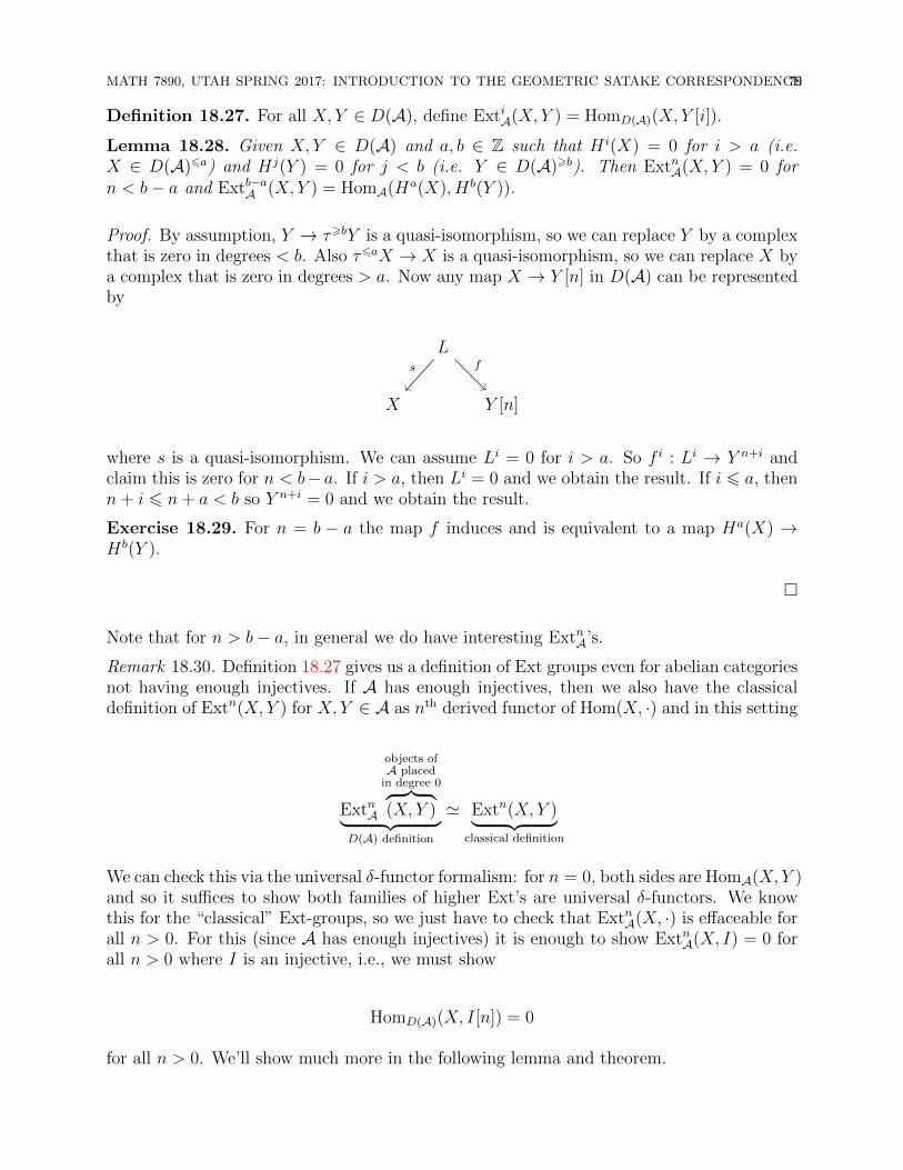
MATH 7890, UTAH SPRING 2017: INTRODUCTION TO THE GEOMETRIC SATAKE CORRESPONDENCE79
Definition 18.27. For all X, Y ∈ D(A), define ExtiA(X, Y ) = HomD(A)(X, Y [i]).
Lemma 18.28. Given X, Y ∈ D(A) and a, b ∈ Z such that H i(X) = 0 for i > a (i.e.X ∈ D(A)6a) and Hj(Y ) = 0 for j < b (i.e. Y ∈ D(A)>b). Then ExtnA(X, Y ) = 0 forn < b− a and Extb−aA (X, Y ) = HomA(Ha(X), Hb(Y )).
Proof. By assumption, Y → τ>bY is a quasi-isomorphism, so we can replace Y by a complexthat is zero in degrees < b. Also τ6aX → X is a quasi-isomorphism, so we can replace X bya complex that is zero in degrees > a. Now any map X → Y [n] in D(A) can be representedby
L
X Y [n]
s f
where s is a quasi-isomorphism. We can assume Li = 0 for i > a. So f i : Li → Y n+i andclaim this is zero for n < b− a. If i > a, then Li = 0 and we obtain the result. If i 6 a, thenn+ i 6 n+ a < b so Y n+i = 0 and we obtain the result.
Exercise 18.29. For n = b − a the map f induces and is equivalent to a map Ha(X) →Hb(Y ).
�
Note that for n > b− a, in general we do have interesting ExtnA’s.
Remark 18.30. Definition 18.27 gives us a definition of Ext groups even for abelian categoriesnot having enough injectives. If A has enough injectives, then we also have the classicaldefinition of Extn(X, Y ) for X, Y ∈ A as nth derived functor of Hom(X, ·) and in this setting
ExtnA
objects ofA placed
in degree 0︷ ︸︸ ︷(X, Y )︸ ︷︷ ︸
D(A) definition
' Extn(X, Y )︸ ︷︷ ︸classical definition
We can check this via the universal δ-functor formalism: for n = 0, both sides are HomA(X, Y )and so it suffices to show both families of higher Ext’s are universal δ-functors. We knowthis for the “classical” Ext-groups, so we just have to check that ExtnA(X, ·) is effaceable forall n > 0. For this (since A has enough injectives) it is enough to show ExtnA(X, I) = 0 forall n > 0 where I is an injective, i.e., we must show
HomD(A)(X, I[n]) = 0
for all n > 0. We’ll show much more in the following lemma and theorem.
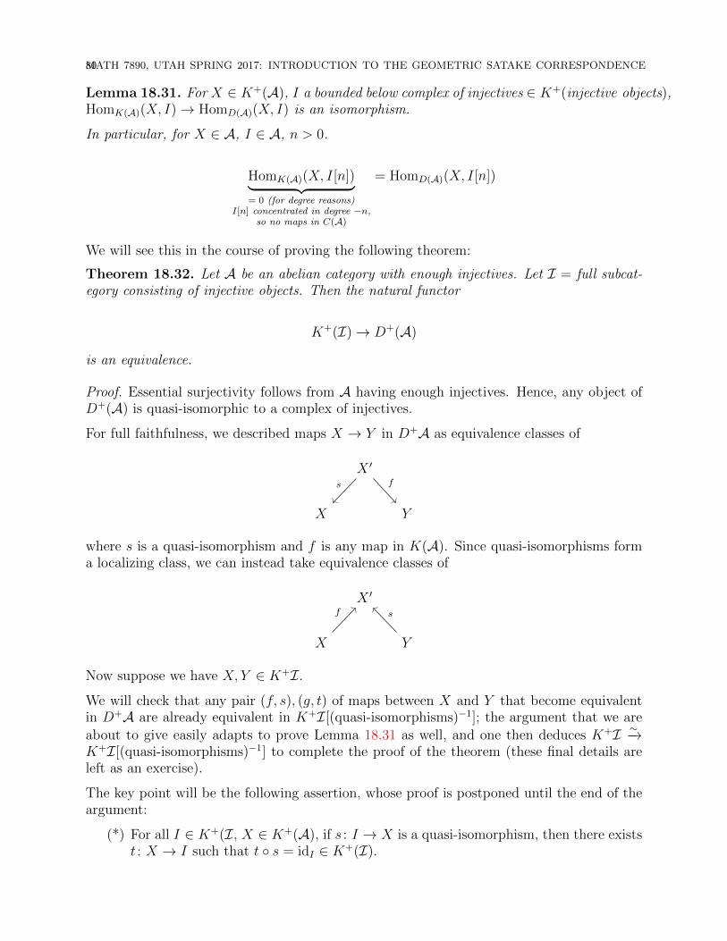
80MATH 7890, UTAH SPRING 2017: INTRODUCTION TO THE GEOMETRIC SATAKE CORRESPONDENCE
Lemma 18.31. For X ∈ K+(A), I a bounded below complex of injectives ∈ K+(injective objects),HomK(A)(X, I)→ HomD(A)(X, I) is an isomorphism.
In particular, for X ∈ A, I ∈ A, n > 0.
HomK(A)(X, I[n])︸ ︷︷ ︸= 0 (for degree reasons)
I[n] concentrated in degree −n,so no maps in C(A)
= HomD(A)(X, I[n])
We will see this in the course of proving the following theorem:
Theorem 18.32. Let A be an abelian category with enough injectives. Let I = full subcat-egory consisting of injective objects. Then the natural functor
K+(I)→ D+(A)
is an equivalence.
Proof. Essential surjectivity follows from A having enough injectives. Hence, any object ofD+(A) is quasi-isomorphic to a complex of injectives.
For full faithfulness, we described maps X → Y in D+A as equivalence classes of
X ′
X Y
s f
where s is a quasi-isomorphism and f is any map in K(A). Since quasi-isomorphisms forma localizing class, we can instead take equivalence classes of
X ′
X Y
f s
Now suppose we have X, Y ∈ K+I.
We will check that any pair (f, s), (g, t) of maps between X and Y that become equivalentin D+A are already equivalent in K+I[(quasi-isomorphisms)−1]; the argument that we are
about to give easily adapts to prove Lemma 18.31 as well, and one then deduces K+I ∼−→K+I[(quasi-isomorphisms)−1] to complete the proof of the theorem (these final details areleft as an exercise).
The key point will be the following assertion, whose proof is postponed until the end of theargument:
(*) For all I ∈ K+(I, X ∈ K+(A), if s : I → X is a quasi-isomorphism, then there existst : X → I such that t ◦ s = idI ∈ K+(I).
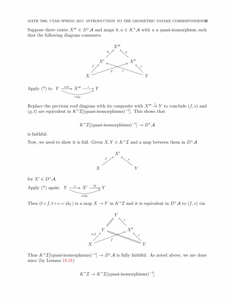
MATH 7890, UTAH SPRING 2017: INTRODUCTION TO THE GEOMETRIC SATAKE CORRESPONDENCE81
Suppose there exists X ′′′ ∈ D+A and maps h, u ∈ K+A with u a quasi-isomorphism suchthat the following diagram commutes
X ′′′
X ′ X ′′
X Y
h u
f
s
t
g
Apply (*) to Y X ′′′ Y
∼idY
u◦t i
Replace the previous roof diagram with its composite with X ′′′i−→ Y to conclude (f, s) and
(g, t) are equivalent in K+I[(quasi-isomorphisms)−1]. This shows that
K+I[(quasi-isomorphisms)−1]→ D+A
is faithful.
Now, we need to show it is full. Given X, Y ∈ K+I and a map between them in D+A
X ′
X Y
f s
for X ′ ∈ D+A.
Apply (*) again: Y X ′ Y
'idY
s ∃t
Then (t ◦ f, t ◦ s = idY ) is a map X → Y in K+I and it is equivalent in D+A to (f, s) via
Y
Y X ′′
X Y
t
t◦f s
f
Thus K+I[(quasi-isomorphisms)−1] → D+A is fully faithful. As noted above, we are donesince (by Lemma 18.31)
K+I → K+I[(quasi-isomorphisms)−1]
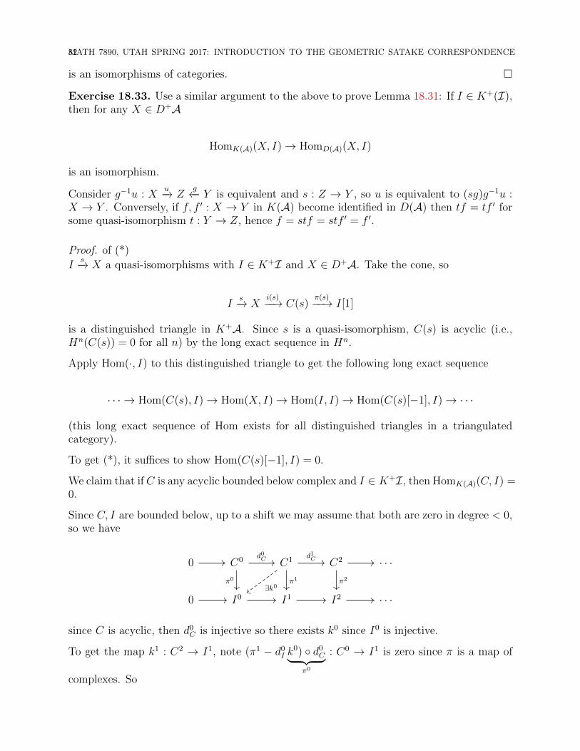
82MATH 7890, UTAH SPRING 2017: INTRODUCTION TO THE GEOMETRIC SATAKE CORRESPONDENCE
is an isomorphisms of categories. �
Exercise 18.33. Use a similar argument to the above to prove Lemma 18.31: If I ∈ K+(I),then for any X ∈ D+A
HomK(A)(X, I)→ HomD(A)(X, I)
is an isomorphism.
Consider g−1u : Xu−→ Z
g←− Y is equivalent and s : Z → Y , so u is equivalent to (sg)g−1u :X → Y . Conversely, if f, f ′ : X → Y in K(A) become identified in D(A) then tf = tf ′ forsome quasi-isomorphism t : Y → Z, hence f = stf = stf ′ = f ′.
Proof. of (*)
Is−→ X a quasi-isomorphisms with I ∈ K+I and X ∈ D+A. Take the cone, so
Is−→ X
i(s)−−→ C(s)π(s)−−→ I[1]
is a distinguished triangle in K+A. Since s is a quasi-isomorphism, C(s) is acyclic (i.e.,Hn(C(s)) = 0 for all n) by the long exact sequence in Hn.
Apply Hom(·, I) to this distinguished triangle to get the following long exact sequence
· · · → Hom(C(s), I)→ Hom(X, I)→ Hom(I, I)→ Hom(C(s)[−1], I)→ · · ·
(this long exact sequence of Hom exists for all distinguished triangles in a triangulatedcategory).
To get (*), it suffices to show Hom(C(s)[−1], I) = 0.
We claim that if C is any acyclic bounded below complex and I ∈ K+I, then HomK(A)(C, I) =0.
Since C, I are bounded below, up to a shift we may assume that both are zero in degree < 0,so we have
0 C0 C1 C2 · · ·
0 I0 I1 I2 · · ·
d0C
π0
d1C
π1
∃k0π2
since C is acyclic, then d0C is injective so there exists k0 since I0 is injective.
To get the map k1 : C2 → I1, note (π1 − d0I k
0) ◦ d0C︸ ︷︷ ︸
π0
: C0 → I1 is zero since π is a map of
complexes. So
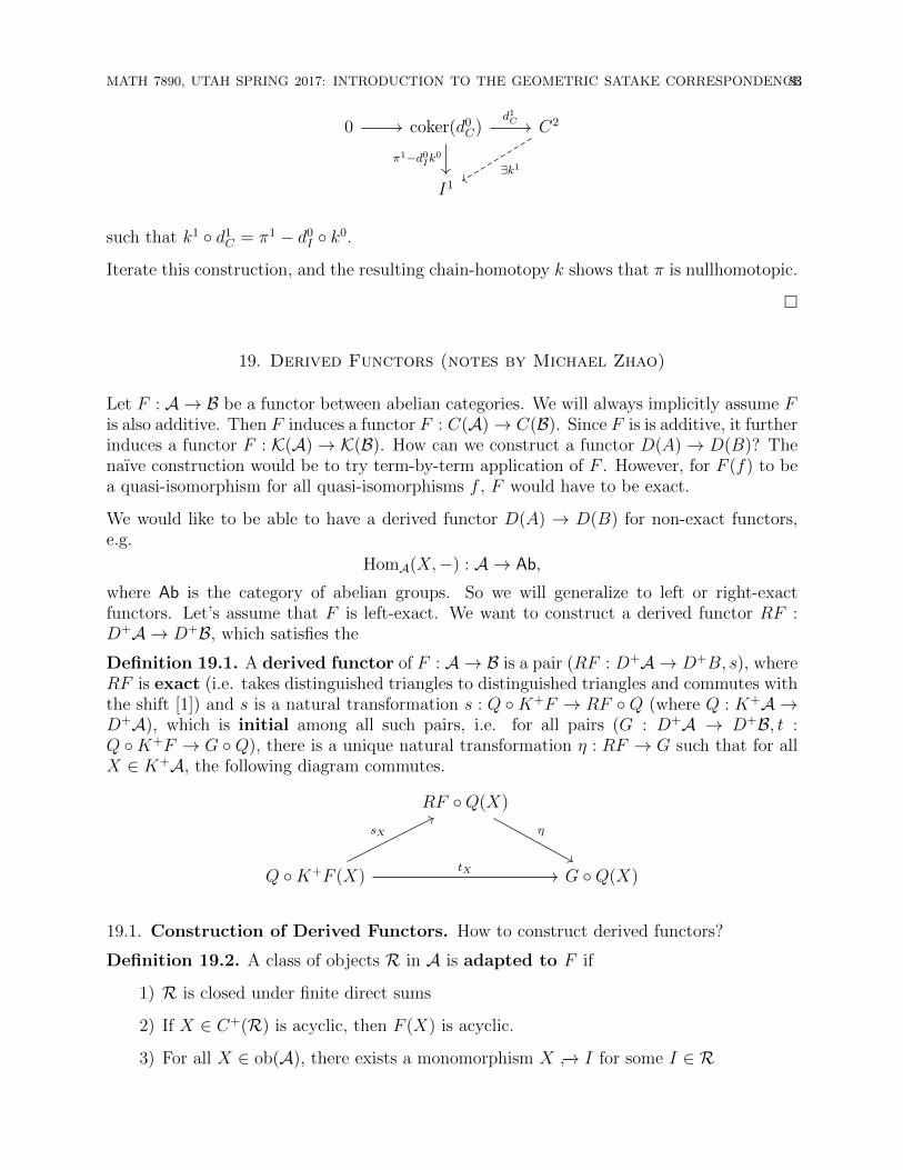
MATH 7890, UTAH SPRING 2017: INTRODUCTION TO THE GEOMETRIC SATAKE CORRESPONDENCE83
0 coker(d0C) C2
I1
d1C
π1−d0Ik
0
∃k1
such that k1 ◦ d1C = π1 − d0
I ◦ k0.
Iterate this construction, and the resulting chain-homotopy k shows that π is nullhomotopic.
�
19. Derived Functors (notes by Michael Zhao)
Let F : A → B be a functor between abelian categories. We will always implicitly assume Fis also additive. Then F induces a functor F : C(A)→ C(B). Since F is is additive, it furtherinduces a functor F : K(A)→ K(B). How can we construct a functor D(A)→ D(B)? Thenaıve construction would be to try term-by-term application of F . However, for F (f) to bea quasi-isomorphism for all quasi-isomorphisms f , F would have to be exact.
We would like to be able to have a derived functor D(A) → D(B) for non-exact functors,e.g.
HomA(X,−) : A → Ab,
where Ab is the category of abelian groups. So we will generalize to left or right-exactfunctors. Let’s assume that F is left-exact. We want to construct a derived functor RF :D+A → D+B, which satisfies the
Definition 19.1. A derived functor of F : A → B is a pair (RF : D+A → D+B, s), whereRF is exact (i.e. takes distinguished triangles to distinguished triangles and commutes withthe shift [1]) and s is a natural transformation s : Q ◦K+F → RF ◦Q (where Q : K+A →D+A), which is initial among all such pairs, i.e. for all pairs (G : D+A → D+B, t :Q ◦K+F → G ◦Q), there is a unique natural transformation η : RF → G such that for allX ∈ K+A, the following diagram commutes.
RF ◦Q(X)
Q ◦K+F (X) G ◦Q(X)
ηsX
tX
19.1. Construction of Derived Functors. How to construct derived functors?
Definition 19.2. A class of objects R in A is adapted to F if
1) R is closed under finite direct sums
2) If X ∈ C+(R) is acyclic, then F (X) is acyclic.
3) For all X ∈ ob(A), there exists a monomorphism X ↪−→ I for some I ∈ R
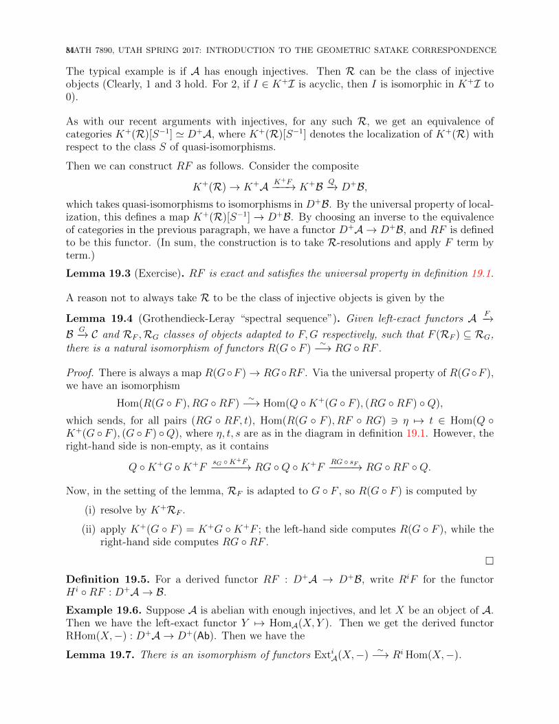
84MATH 7890, UTAH SPRING 2017: INTRODUCTION TO THE GEOMETRIC SATAKE CORRESPONDENCE
The typical example is if A has enough injectives. Then R can be the class of injectiveobjects (Clearly, 1 and 3 hold. For 2, if I ∈ K+I is acyclic, then I is isomorphic in K+I to0).
As with our recent arguments with injectives, for any such R, we get an equivalence ofcategories K+(R)[S−1] ' D+A, where K+(R)[S−1] denotes the localization of K+(R) withrespect to the class S of quasi-isomorphisms.
Then we can construct RF as follows. Consider the composite
K+(R)→ K+A K+F−−−→ K+B Q−→ D+B,which takes quasi-isomorphisms to isomorphisms in D+B. By the universal property of local-ization, this defines a map K+(R)[S−1]→ D+B. By choosing an inverse to the equivalenceof categories in the previous paragraph, we have a functor D+A → D+B, and RF is definedto be this functor. (In sum, the construction is to take R-resolutions and apply F term byterm.)
Lemma 19.3 (Exercise). RF is exact and satisfies the universal property in definition 19.1.
A reason not to always take R to be the class of injective objects is given by the
Lemma 19.4 (Grothendieck-Leray “spectral sequence”). Given left-exact functors A F−→B G−→ C and RF ,RG classes of objects adapted to F,G respectively, such that F (RF ) ⊆ RG,
there is a natural isomorphism of functors R(G ◦ F )∼−→ RG ◦RF .
Proof. There is always a map R(G◦F )→ RG◦RF . Via the universal property of R(G◦F ),we have an isomorphism
Hom(R(G ◦ F ), RG ◦RF )∼−→ Hom(Q ◦K+(G ◦ F ), (RG ◦RF ) ◦Q),
which sends, for all pairs (RG ◦ RF, t), Hom(R(G ◦ F ), RF ◦ RG) 3 η 7→ t ∈ Hom(Q ◦K+(G ◦ F ), (G ◦ F ) ◦Q), where η, t, s are as in the diagram in definition 19.1. However, theright-hand side is non-empty, as it contains
Q ◦K+G ◦K+FsG ◦K+F−−−−−→ RG ◦Q ◦K+F
RG ◦ sF−−−−→ RG ◦RF ◦Q.
Now, in the setting of the lemma, RF is adapted to G ◦ F , so R(G ◦ F ) is computed by
(i) resolve by K+RF .
(ii) apply K+(G ◦ F ) = K+G ◦K+F ; the left-hand side computes R(G ◦ F ), while theright-hand side computes RG ◦RF .
�
Definition 19.5. For a derived functor RF : D+A → D+B, write RiF for the functorH i ◦RF : D+A → B.
Example 19.6. Suppose A is abelian with enough injectives, and let X be an object of A.Then we have the left-exact functor Y 7→ HomA(X, Y ). Then we get the derived functorRHom(X,−) : D+A → D+(Ab). Then we have the
Lemma 19.7. There is an isomorphism of functors ExtiA(X,−)∼−→ Ri Hom(X,−).
MATH 7890, UTAH SPRING 2017: INTRODUCTION TO THE GEOMETRIC SATAKE CORRESPONDENCE85
We will actually give a more general construction, similar to this one, which allows forX ∈ DA. Define a functor
Hom•A( , ) : C(A)op × C+(A)→ C(Ab)
by
HomnA(X, Y ) =
∏i∈Z
HomA(X i, Y i+n),
withdn((f i : X i → Y i+n)i∈Z) = dY ◦ f i + (−1)n+1f i+1 ◦ dX ,
which is a map from X i → Y i+n+1. (Check that d2 = 0.)
A key property of Hom•A is that it computes HomK(A):
Z0(Hom•A(X, Y )) = {(f i : X i → Y i) | dY f = fdX} = HomC(A)(X, Y ),
and
B0(Hom•A(X, Y )) = {(gi : X i → Y i)i∈Z | ∃fi : X i → Y i−1, g = dY f + fdX},which is the set of null-homotopic chain maps. Then H0(Hom•A(X, Y )) = HomK(A)(X, Y ).
Proposition 19.8. There exists a bifunctor RHom : D(A)op ×D+(A)→ D(Ab) extendingthe previously defined RHom : Aop ×D+(A)→ D(Ab), given by
RHom(X, Y ) := Hom•(X, I),
for a given quasi-isomorphism Y−→∼ I, where I is a complex of injectives. Moreover, for any
X, Y ,H i(RHom(X, Y )) = HomD(A)(X, Y [i]).
Proof. We need to check that RHom is well-defined and functorial. Note that for any Yf−→ Z
(in C+(A)) and injective resolutions α : Y−→∼ I, Ψ : Z
−→∼ J , there exists a unique f ′ inK(A) such that the following diagram commutes in K(A) (not in C(A)!).
Y Z
I J
α
f
Ψ
f ′
To see this, apply HomK(A)(−, J) to the distinguished triangle
Yα−→ I → C(α)→ Y [1].
Note that C(α) is acyclic, and we showed that HomK+(A)(M,N) = 0 if M is acyclic and Nis a complex of injectives. Thus we have a bijection
HomK(A)(I, J)∼−→ HomK(A)(Y, J),
The desired f ′ : I → J is then the preimage of Ψ ◦ f under this isomorphism. By post-composition with f ′ we get the map RHom(X, Y )→ RHom(X,Z).
Exercise 19.9. If you change f ′ by something null-homotopic, then the induced map
Hom•(X, I)→ Hom•(X, J)
changes by something null-homotopic.
86MATH 7890, UTAH SPRING 2017: INTRODUCTION TO THE GEOMETRIC SATAKE CORRESPONDENCE
Now we check that this extends the previous RHom : Aop ×D+(A) → D(Ab). Previously,
for X ∈ A, Y ∈ D+(A) and α : Y−→∼ I an injective resolution, we had RHom(X, Y )old =
HomA(X, I•). On the other hand, the version just defined is
RHom(X, Y )new = Hom•(X, I),
which equals ∏i∈Z
Hom(X i, I i+n) = Hom(X, In),
in degree n. There is an obvious quasi-isomorphism between these two versions of RHom.
Finally, we show that
H0(RHom(X, Y )) = HomD(A)(X, Y ). (1)
Let α : Y−→∼ I be an injective resolution. By definition,
H0(RHom(X, Y )) = H0(Hom•(X, I)) = HomK(A)(X, I) = HomD(A)(X, I) ' HomD(A)(X, Y ),
where the second to last equality follows relies on I being a complex of injectives (Lemma18.31).
�
20. Sheaf Cohomology (notes by Michael Zhao)
Everything we discuss will have an analog in etale topology, but we will work in the settingof classical topology where everything is more down-to-earth. Our main aim is to developthe formalism of the “six operations” between derived categories of sheaves on topologicalspaces.
Let X be a topological space. Let R be a commutative ring. Let ShR(X) denote thecategory of sheaves of R-modules. We may also leave R implicit, and just write Sh(X).Let D(X) := D(Sh(X)) denote the derived category of Sh(X), and likewise for its boundedvariants. We are interested in the induced maps on or between D(X) by maps of topologicalspaces.
Example 20.1 (Direct and Inverse Image). Let f : X → Y be a map of topological spaces.Let F ∈ Sh(X). Define f∗F ∈ Sh(Y ) by f∗F(U) := F(f−1(U)). This provides a functorf∗ : Sh(X)→ Sh(Y ).
Define, for G ∈ Sh(Y ), f−1G ∈ Sh(X) as the sheafification of the presheaf
(f−1G)#(V ) = limU⊃f(V )
G(U).
Reminder. Sheafification and the forgetful functor which takes a sheaf and returns theunderlying presheaf are left and right adjoints, respectively.
Lemma 20.2 (Exercise). f−1 is left adjoint to f∗ for all f : X → Y .
MATH 7890, UTAH SPRING 2017: INTRODUCTION TO THE GEOMETRIC SATAKE CORRESPONDENCE87
Whenever we have F right adjoint to G, there are natural transformations
1ε−→ F ◦G
G ◦ F η−→ 1,
which are respectively called the unit and counit of the adjunction.
Exercise 20.3. For f−1 and f∗, write down ε, η.
Lemma 20.4 (Exercise).
(1) All left-adjoints are right-exact.
(2) All right-adjoints are left-exact.
(3) f−1 is exact.
(4) f∗ preserves injectives, since it has an exact left-adjoint.
Since f−1 is exact, we get an induced functor f−1 : D(Y ) → D(X) by the naıve definition.Since f∗ is left-exact and Sh(X) has enough injectives, get Rf∗ : D+(X)→ D+(Y ).
Corollary 20.5.
(1) There exists an adjunction isomorphism RHom(f−1K,L) ' RHom(K,Rf∗L) forK ∈ D+(Y ), L ∈ D+(X).
(2) Apply H0 to (1) to get the adjunction
HomD+(X)(f−1K,L) ' HomD+(Y )(K,Rf∗L).
Remark 20.6. This is the first adjoint pair of the six operations.
Proof. (2) comes from the formula (1) applied to part (1) of the corollary, so we just need
to show (1). Let L−→∼ I be an injective resolution. Then Rf∗L = f∗I and
RHom(K, f∗I) = Hom•(K, f∗I) = Hom•(f−1K, I) = RHom(f−1K, I) = RHom(f−1K,L).
�
20.1. Internal Hom. We can enrich these adjuctions using the internal hom on Sh(X),which is a functor
Hom : Sh(X)op × Sh(X)→ Sh(X),
given byHom(F ,G)(U) = HomSh(U)(F
∣∣U,G∣∣U
) ∈ Ab.
(Check that Hom(F ,G)) is a sheaf.) Then Hom(F ,−) is a left-exact functor Sh(X) →Sh(X), so we get its derived functor
RHom(F ,−) : D+(X)→ D+(X).
As with our extension of RHom from Aop ×D+(A)→ D(Ab) to D(A)×D+(A)→ D(Ab),we can extend RHom to a bifunctor RHom : D(X)op ×D+(X)→ D(X). As before, defineHom•(K,L) by
Homn(K,L) =∏i∈Z
Hom(Ki, Li+n),
88MATH 7890, UTAH SPRING 2017: INTRODUCTION TO THE GEOMETRIC SATAKE CORRESPONDENCE
and proceed as with RHom.
Theorem 20.7 (Formula for Global Sections Derived Functor). For all K ∈ D−(X), L ∈D+(X), there are natural isomorphisms
RΓ(RHom(K,L))∼−→ RHom(K,L),
where RΓ : D+(X) → D+(Ab) is the derived functor of global sections Γ : Sh(X) → Ab(alternatively, RΓ = Rπ∗ for the terminal map π : X → ∗).
Proof. Let L−→∼ I be an injective resolution. Then RHom(K,L) = Hom•(K, I). Note that
this complex is bounded below. The terms of Hom•(K, I) need not be injective, but theystill belong to a class of sheaves adapted to Γ, namely the flasque sheaves.
Definition 20.8. F ∈ Sh(X) is flasque or flabby if for all opens U ⊃ V , F(U)� F(V ).
Lemma 20.9.
(1) The class of flasque sheaves is adapted to the left-exact functor Γ.
(2) For any F and for an injective I ∈ Sh(X), Hom(F , I) is flasque.
(3) Injective sheaves are flasque.
Granted this lemma, we then have
RΓ(RHom(K,L)) = Γ(X,Hom•(K, I)) = Hom•(K, I) = RHom(K,L).
(Given the lemma, this is the spectral sequence for composite derived functors.) �
Remark 20.10 (On (1) of Lemma 20.9). Need to know that
(a) Flasque sheaves are stable under direct sums.
(b) Every sheaf injects into a flasque one: given F ∈ Sh(X), form J ∈ Sh(X) withJ(U) =
∏x∈U Fx. Then F ↪−→ J and J is flasque.
(c) Γ(X,N) is acyclic for N ∈ C+(flasque sheaves). The main point is to show that ifthere is the short exact sequence
0→ F → G → H → 0
with F flasque, then G(X)� H(X).
21. Perverse Sheaves (Christian Klevdal)
The original reference for this topic the paper by Beilinson-Bernstein-Deligne (BBD) ”Fais-ceux pervers”. The name perverse sheaf is somewhat misleading since they are not honestsheaves, rather they live in Db
c(X), the bounded derived category of constructible sheaves ona topological space. In what follows, we will either take X to be a variety over the complexnumbers in the classical (analytic) topology, or a variety over any perfect field k, in the etaletopology.
Perverse sheaves are the heart of a non-standard t-structure on Dbc(X). Recall that for an
abelian category A, the standard t-structure on D(A) takes D≤0, respectively D≥0 to bethe complexes K with H i(K) = 0 for i > 0, respectively i < 0. Before getting down to
MATH 7890, UTAH SPRING 2017: INTRODUCTION TO THE GEOMETRIC SATAKE CORRESPONDENCE89
the specific case of perverse sheaves, we recall the definition and some generalities aboutt-structures.
Definition 21.1. A t-structure on a triangulated category D is a pair (D≤0,D≥0) of fullsubcategories where (with the notation D≥n = D≥0[−n] and likewise for D≤n) we have:
(1) D≤0 ⊂ D≤1 and D≥1 ⊂ D≥0.
(2) HomD(D≤0,D≥1) = 0.
(3) For all X ∈ D, there exists a distinguished triangle
Y → X → Z → Y [1]
with Y ∈ D≤0 and Z ∈ D≥1.
Recall that in the case of D(A) and the standard t-structure we had truncation functors
τ≤n : D(A)→ D(A)≤n K 7→ · · · → Kn−1 → ker(dn)→ 0→ · · ·τ≥n : D(A)→ D(A)≥n K 7→ · · · → 0→ coker(dn)→ Kn+1 → · · ·
and we used these functors to show the existence of the distinguished triangle in axiom 3 ofa t-structure. Our next step is to show that given any t-structure, such truncation functorsalways exist.
Proposition 21.2. Let (D≤0,D≥0) be a t-structure on a triangulated category D. Then
(1) There exists a left adjoint τ≥n for the inclusion D≥n → D and a right adjoint τ≤n
for the inclusion D≤n → D.
(2) For all X ∈ D there exists a unique δX : τ≥n+1X → τ≤nX[1] such that
τ≤nX → X → τ≥nXδX−→ τ≤nX[1]
is a distinguished triangle (the maps to and from X are the canonical maps fromadjunction).
Proof. First, we may assume n = 0. By (3) from the definition of a t-structure, there existssome distinguished triangle
X≤0 → X → X≥1 → X≤0[1]
with X≤0 ∈ D≤0 and X≥1 ∈ D≥1. If Y is in D≤0 we apply Hom(Y, ·) to the above exacttriangle and get an exact sequence
Hom(Y,X≥1[−1])→ Hom(Y,X)→ Hom(Y,X≤0)→ Hom(Y,X≥1)
But we know that the first and last terms of the sequence are zero from properties (1), (2)of a t-structure. Defining τ≤0X = X≤0 we get the required isomorphism. However, we needto check that this definition of τ≤0 gives a well defined functor, and that τ≤0 is the rightadjoint of inclusion (i.e. that the isomorphisms given above are functorial). It is sufficientto show for each map X → X ′ in D that there is a unique factorization
90MATH 7890, UTAH SPRING 2017: INTRODUCTION TO THE GEOMETRIC SATAKE CORRESPONDENCE
τ≤0X τ≤0X ′
X X ′
∃!
To see the unique factorization, consider the exact triangle τ≤0X ′ → X ′ → X ′≥1 → (τ≤0X ′)[1].
Applying Hom(τ≤0X, ·) we get an exact sequence
Hom(τ≤0X,X ′≥1[−1])→ Hom(τ≤0X,X ′)→ Hom(τ≤0X, τ≤0X ′)→ Hom(τ≤0X,X ′≥1)
Again the first and last terms vanish. Thus the middle arrow is an isomorphism and we geta unique factorization as required. If we define τ≥1X = X≥1 a similar proof shows that thisis a well defined functor that is left adjoint to inclusion.
The second claim follows from the following lemma. �
Lemma 21.3. Suppose we are given maps δ1, δ2 such that A→ X → Bδi−→ A[1] is an exact
triangle for i = 1, 2. Then δ1 = δ2 if Hom(A[1], B) = 0.
Proof. Consider the diagram
A X B A[1]
A X B A[1]
a
id
b
id
δ1
f id
a b δ2
The existence of the dotted arrow making this a morphism of triangles follows from theaxioms of a triangulated category. Our aim is to show that f = idB. Now we have thatfb = b or equivalently (idB − f)b = 0. Applying Hom(·, B) to the top row we get an exactsequence
0 = Hom(A[1], B)→ Hom(B,B)→ Hom(X,B)
Clearly f − idB maps to zero in the last Hom set. Since the map is injective, we concludethat f = idB as required. �
Definition 21.4. Let D be a triangluated category and (D≤0,D≥0) a t-structure on D. Theheart of this t-structure is D♥ = D≤0 ∩ D≥0.
We can define cohomology a cohomology functor H0 : D → D♥ with respect to this t-structure to be the composition τ≤0 ◦ τ≥0(' τ≥0 ◦ τ≤0. Likewise, we define Hn = H0 ◦ [n].
Example 21.5. If A is an abelian category we can give D(A) the standard t-structure(where D≤0, resp. D≥0, consists of those complexes with zero cohomology in degree i > 0,resp. i < 0). In this case, the heart of this t-structure can be naturally identified with A (byconsider objects as chain complexes concentrated in degree 0); and the cohomology functoris just the usual cohomology of a chain complex.
Note that in the above example, the heart of the t-structure is an abelian category. Surpris-ingly, this turns out to be true in general.
MATH 7890, UTAH SPRING 2017: INTRODUCTION TO THE GEOMETRIC SATAKE CORRESPONDENCE91
Theorem 21.6. (BBD) For any t-structure on a triangulated category D, the heart D♥ isan abelian category.
The next natural question is what can we say about D♥? One thing that holds is that forA,B ∈ D♥ one has Ext1
D♥(A,B) ∼= Hom(A,B[1]). We caution that the analogue does nothold for higher exts.
Example 21.7. Suppose X is a (reasonable) topological space, and let
D = Dloc(X) = {K ∈ D(X) : H i(K) is locally constant for all i}.The standard t-structure on D(X) induces a t-structure on D. If X is connected and simplyconnected, then locally constant sheaves are constant, hence D♥ is equivalent to the categoryAb of abelian groups. Thus if n > 1
ExtnD♥(Z,Z) ∼= ExtnAb(Z,Z) = 0
However,
HomD(ZX ,ZX [n]) = H0RHom(ZX ,ZX [n]) = H0RΓ(X,ZX [n]) = Hn(X,Z)
So if X is simply connected but has higher cohomology (eg, X = S2), we see that D(D♥) isnot equivalent to Dloc(X).
However, in the cases we are interested in, we have the following
Theorem 21.8. (Nori) If X/k is a quasi-projective variety, then Dbc(X) is equivalent to the
bounded derived category of the abelian category of constructible sheaves on X. (Beilinson)These are equivalent to the bounded derived category of the abelian category of perversesheaves on X.
Both of these assertions have geometric content!
Before defining the perverse t-structure, we make a couple more general definitions. Firstrecall (excercise):
Theorem 21.9. For any t-structure (D≤0,D≥0) on a triangulated category D, the cohomol-ogy functor H0 : D → D♥ is a cohomological functor (meaning it takes distinguished trianglesto long exact sequences).
Definition 21.10. Lef F : D1 → D2 be exact functors of triangulated categories (meaningthat F commutes with the shift and preserves distinguished triangles). Suppose we have t-structures (D≤0
i ,D≥0i ) on Di for i = 1, 2. Then we say that F is t-left exact if F (D≥0
1 ) ⊂ D≥02
and that F is t-right exact if F (D≤01 ) ⊂ D≤0
2 . We say that F is t-exact if it is both t-left andt-right exact.
In the setting of the definition (with out any assumptions on the t-exactness of F ), we definea functor F♥ : D♥1 → D♥2 by the composition
D♥1 ⊂ D1F−→ D2
H0
−→ D♥2As a remark, in BBD, F♥ is denoted pF . We may later lapse into this notation.
Before defining the perverse t-structure (whose heart will be the category of perverse sheaves)we begin with a little motivation. The source of the theory is intersection cohomology
92MATH 7890, UTAH SPRING 2017: INTRODUCTION TO THE GEOMETRIC SATAKE CORRESPONDENCE
IH∗(X) which for a variety X is defined as H∗(X, ICX) where ICX is a particular perversesheaf on X called the intersection complex. Here are some of the good features of IH∗(X).
(1) IH∗(X) = H∗(X) if X is smooth.
(2) IH∗(X) always satisfies Poincare duality (ifX is not projective, you need the compactsupports version–we’ll see this later).
(3) For any projective X, IHm(X) is pure of weight m, either in the sense of Hodgetheory (k = C) or Frobenius eigenvalues (k = Fq).
Let’s elaborate on this last point. In the case that X/C is smooth and projective, Hm(X,Q)is naturally endowed with a pure Hodge structure of weight m. However if X is projective butnot smooth, Hm(X,Q) has a mixed Hodge structure of weights ≤ m. In the case that X/Fqis smooth and projective, then the action of Frobenius on Hm
et (XFq ,Q`) is pure of weight m,
meaning all eigenvalues are algebraic numbers with archimedean absolute values qm/2. If wedon’t assume X is smooth, then the etale cohomology is mixed with weights ≤ m. Whatthe final point above is saying is that when X is projective, but possibly singular, IHm(X)is pure of weight m in the appropriate sense.
We now define the perverse t-structure. In this setting, let k be a perfect field, X/k aseparated scheme of finite type over k (which we may assume is reduced). We write D(X) forDbc(X) the subcategory of the bounded derived category of sheaves on X with constructible
cohomology.
Definition 21.11. We define full subcategories of D(X) by
pD≤0(X) = {K ∈ D(X) : dim(suppH iK) ≤ −i, ∀i}pD≥0(X) = {K ∈ D(X) : dim(suppH i(DXK)) ≤ −i, ∀i}
(Recall that DXK = RHom(K, π!Q`) for π : X → Speck).
This is the “self-dual” (for reasons we will see) or “middle” perversity. There are variantswhere one changes the numerics of the above definition, but this is the version of centralimportance in algebraic geometry.
Example 21.12. If X is smooth, dimension d and F a local system on X then F [d] ∈pD≥0∩ pD≤0. To see that it is in pD≤0 note that H i(F [d]) is non zero only in degree d, whereit has full support. The dual statement will follow from Lemma 21.16
Definition 21.13. The category of perverse sheaves on X is Perv(X) = pD≥0 ∩ pD≤0.
Theorem 21.14. (pD≤0(X), pD≥0(X)) is a t-structure on D(X) with heart Perv(X).
This theorem is proven by induction on the dimension of X, using the BBD technique of glu-ing abstract t-structures. In addition to this formalism, we will have to know what happensin “the smooth case.” We define Dloc(X) = {K ∈ D(X) : H i(X) is locally constant ∀i}, andwe next show that when X is smooth, the perverse t-structure on Dloc(X) is just a translateof the standard t-structure.
Proposition 21.15. If U is smooth of dimension d then
(pD≤0(U) ∩Dloc(U), pD≥0(U) ∩Dloc(U)) = (D≤−dloc (U), D≥−dloc (U))
MATH 7890, UTAH SPRING 2017: INTRODUCTION TO THE GEOMETRIC SATAKE CORRESPONDENCE93
(a shift of the standard t-structure).
Proof. For K ∈ Dloc(U) if H−iK 6= 0 then suppH−iK = U since the cohomology is a localsystem. Thus the condition K ∈ pD≤0(U)∩Dloc(U) is equivalent to H iK = 0 for all i > −d.
Hence pD≤0(U) ∩ Dloc(U) = D≤−dloc (U). On the other hand K ∈ pD≥0(U) if and only ifDUK ∈ pD≤0(U) which is equivalant to saying H i(DUK) = 0 for all i > −d. The followinglemma shows that this is equivalent to having HjK = 0 for all j < −d. �
Lemma 21.16. If U is smooth of dimension d and K ∈ Dloc(U) then for all i
H i(DUK) ∼= H−i−2d(K)∨(d)
(where the (d) is a Tate twist in case we are working with etale cohomology).
Proof. Proceed by induction on |{i : H iK 6= 0}|. Given K let n be the maximal index suchthat HnK 6= 0. We get a distinguished triangle
τ≤n−1K → K → τ≥nK+1−→
Since n is maximal, we know that τ≥nK ∼= HnK[−n]. Write F = HnK. Now we applyRHom(·,KU) = DU and take the long exact sequence of the resulting distinguished triangle.Since U is smooth we have KU = Q`[2d](d) and the long exact sequence is
· · · → H i(RHom(F [−n],Q`[2d]))→ H i(RHom(K,Q`[2d]))→ H i(RHom(τ≤n−1K,Q`[2d]))→ · · ·Note that the first term can be can be computed as
H i+n+2dRHom(F ,Q`) =
{0 if i 6= −n− 2d
F∨ if i = −n− 2d
since F is locally constant (if F is constant, i.e. Q`, then Hom(Q`, ·) is the identity functorso there are no higher derived functors; since F is locally constant we can reduce to thiscase). This implies that
H iRHom(K,Q`[2d]) =
F∨ if i = −2d− nH i(DUτ
≤n−1K) if i > −2d− n0 if i < −2d− n
(Check the details as an exercise. For instance,
H iRHom(τ≤n−1K,Q`[2d]) = H0RHom(τ≤n−1K,Q`[2d+ i]),
so if i ≤ −2d−n, i.e. −2d− i ≥ n, then this group vanishes for degree reasons.) The lemmanow follows by applying the induction hypothesis to τ≤n−1K. �
The following important lemma gives a way to describe pD≤0(X) and pD≥0(X) in terms ofrestricting to a decomposition X = U t Z. It motivates the abstract glueing procedure fort-structures to be described in the next section.
Lemma 21.17. Let X/k be separated of finite type. Let j : U → X be an open imbeddingwith closed complement i : Z → X, and let K ∈ D(X). then
• K ∈ pD≤0(X) if and only if j∗K ∈ pD≤0(U) and i∗K ∈ pD≤0(Z); and
• K ∈ pD≥0(X) if and only if j∗K ∈ pD≥0(U) and i!K ∈ pD≥0(Z).
94MATH 7890, UTAH SPRING 2017: INTRODUCTION TO THE GEOMETRIC SATAKE CORRESPONDENCE
Proof. Since i∗ and j∗ are exact for the standard t-structure, Supp(HnK) = Supp(j∗Hn(K))tSupp(i∗Hn(K)). The first item follows. For the second, K ∈ pD≥0(X) ⇐⇒ DX(K) ∈pD≤0(X), which holds (by the first part) if and only if j∗DX(K) ∈ pD≤0(U) and i∗DX(K) ∈pD≤0(Z). Since j∗DX ' DUj
! and i∗DX ' DZi!, the second item follows from the definitions
of the perverse “t-structures” (not yet) on U and Z. �
22. t-structures and gluing (Notes by Sabine Lang)
In this lecture we explain how to glue t-structures. Following BBD, we axiomatize thesituation. Let D, DU , and DZ be triangulated categories equipped with exact (i.e. pre-serving shifts and distinguished triangles) functors i∗ : DZ → D and j∗ : D → DU . Set (forconvenience) i! = i∗ and j! = j∗. Assume the following “glueing axioms” hold:
(G1) i∗ admits a left adjoint i∗ and a right adjoint i!. j∗ admits a left adjoint j! and a rightadjoint j∗.
(G2) j∗i∗ = 0. (By adjunction and Yoneda, we deduce from this i∗j! = 0 and i!j∗ = 0; forinstance,
Hom(i∗j!K,L) = Hom(j!K, i∗L) = Hom(K, j∗i∗L) = 0.)
(G3) For all K ∈ D, there are distinguished triangles (with the adjunction maps)
j!j∗K → K → i∗i
∗K+1−→
and
i∗i!K → K → j∗j
∗K+1−→ .
(G4) j!, i∗, and j∗ are fully faithful. (Exercise: deduce from this that the natural transfor-mations j∗j∗ → id, id→ j∗j!, i
∗i∗ → id, id→ i!i∗ are all isomorphisms.)
Before proceeding with the formalism, we check that the glueing axioms hold in the settingof sheaf theory:
Proposition 22.1. Working in the sheaf theory setting, let U ⊂ X be open, Z = X\U , anddenote by j : U → X, i : Z → X the inclusions. Then the axioms G1 to G4 are all satisfiedby the associated (derived) functors, taking D = Db
c(X), DU = Dbc(U) and DZ = Db
c(Z).
Proof. • G1 : We have seen it before.
• G2 : It is clear from stalks.
• G3 : For the first triangle, for F ∈ Sh(X), we already have that
0→ j!j∗F → F → i∗i
∗F → 0
is exact, by looking at stalks. The functors j!, j∗, i∗ and i∗ are all exacts, so for
K ∈ Dbc(X), we can compute Rj!j
∗K, etc . . . just by applying the functors term byterm. We get a short exact sequence of complexes :
0→ j!j∗K → K → i∗i
∗K → 0,
and this gives rise to an associated distinguished triangle in Dbc(X).
MATH 7890, UTAH SPRING 2017: INTRODUCTION TO THE GEOMETRIC SATAKE CORRESPONDENCE95
For the second triangle, for all F ∈ Sh(X), we have an exact sequence
0→ i∗i!F → F → j∗j
∗F .Moreover, if F is injective, the last map is surjective (see our discussion of cohomologywith supports). So for a general K ∈ Db
c(X), we take an injective replacement andapply this to get the distinguished triangle
i∗Ri!K → K → Rj∗j
∗K+1→ .
• G4 : We have seen some of this. For example, for Rj∗, we have HomD(X)(Rj∗K,Rj ∗L) = HomD(X)(j
∗Rj∗K,L) = HomD(X)(K,L).
�
Theorem 22.2. Let D, DU , DZ, i∗, j∗ be as in the gluing axiomatics. Let (D≤0
U ,D≥0U ) and
(D≤0Z ,D≥0
Z ) be t-structures on DU and DZ. Define
• D≤0 = {K ∈ D | j∗K ∈ D≤0U , i∗K ∈ D≤0
Z },
• D≥0 = {K ∈ D | j!K ∈ D≥0U , i!K ∈ D≥0
Z }.
Then (D≤0,D≥0) is a t-structure on D.
Proof. We need to check three things :
(1) D≤0 ⊂ D≤1 and D≥0 ⊃ D≥1,
(2) Hom(D≤0,D≥1) = 0,
(3) for all X ∈ D, there exists X≤0 ∈ D≤0 and X≥1 ∈ D≥1 so that we have a distinguished
triangle X≤0 → X → X≥1+1→.
We use the following arguments :
(1) Clear.
(2) Let X ∈ D≤0, Y ∈ D≥1. We have a distinguished triangle
j!j∗X → X → i∗i
∗X+1→ .
Applying Hom(−, Y ), we get the long exact sequence
· · · ← Hom(j!j∗X, Y )← Hom(X, Y )← Hom(i∗i
∗X, Y )← . . . .
But we get Hom(j!j∗X, Y ) = HomDU (j∗X, j∗Y ) = 0 by the t-structure on U since
j∗X ∈ D≤0U and j∗Y ∈ D≥1
U . Similarly, Hom(i∗i∗X, Y ) = HomDZ (i∗X, i!Y ) = 0 using
the t-structure on Z and i∗X ∈ D≤0Z , i!Y ∈ D≥1
Z . So this shows that Hom(X, Y ) = 0.
(3) The t-structures on DU , DZ give rise to the associated truncation functors τ≤nU , τ≥nU ,
τ≤nZ , τ≥nZ . For all X ∈ D, we have a map X → j∗τ≥1U j∗X given by the composition
X → j∗j∗X → j∗τ
≥1U j∗X. We can complete this composite to a distinguished triangle
in D : Y → X → j∗τ≥1U j∗X
+1→. Likewise, we have a map Y → i∗τ≥1Z i∗Y from the
composition Y → i∗i∗Y → i∗τ
≥1Z i∗Y . We obtain a distinguished triangle A → Y →
i∗τ≥1Z i∗Y
+1→. Also, A→ Y → X gives a distinguished triangle A→ X → B+1→ .
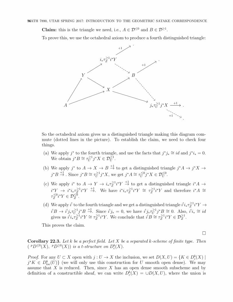
96MATH 7890, UTAH SPRING 2017: INTRODUCTION TO THE GEOMETRIC SATAKE CORRESPONDENCE
Claim: this is the triangle we need, i.e., A ∈ D≤0 and B ∈ D≥1.
To prove this, we use the octahedral axiom to produce a fourth distinguished triangle:
.
i∗τ≥1Z i∗Y .
Y B
X
A j∗τ≥1U j∗X .
.
+1
+1
+1
+1
So the octahedral axiom gives us a distinguished triangle making this diagram com-mute (dotted lines in the picture). To establish the claim, we need to check fourthings.
(a) We apply j∗ to the fourth triangle, and use the facts that j∗j∗ ∼= id and j∗i∗ = 0.We obtain j∗B ∼= τ≥1
U j∗X ∈ D≥1U .
(b) We apply j∗ to A → X → B+1→ to get a distinguished triangle j∗A → j∗X →
j∗B+1→ . Since j∗B ∼= τ≥1
U j∗X, we get j∗A ∼= τ≤0U j∗X ∈ D≤0
U .
(c) We apply i∗ to A → Y → i∗τ≥1Z i∗Y
+1→ to get a distinguished triangle i∗A →i∗Y → i∗i∗τ
≥1Z i∗Y
+1→. We have i∗i∗τ≥1Z i∗Y ∼= τ≥1
Z i∗Y and therefore i∗A ∼=τ≤0Z i∗Y ∈ D≤0
Z .
(d) We apply i! to the fourth triangle and we get a distinguished triangle i!i∗τ≥1Z i∗Y →
i!B → i!j∗τ≥1U j∗B
+1→. Since i!j∗ = 0, we have i!j∗τ≥1U j∗B ∼= 0. Also, i!i∗ ∼= id
gives us i!i∗τ≥1Z i∗Y ∼= τ≥1
Z i∗Y . We conclude that i!B ∼= τ≥1Z i∗Y ∈ D≥1
Z .
This proves the claim.
�
Corollary 22.3. Let k be a perfect field. Let X be a separated k-scheme of finite type. Then( pD≤0(X), pD≥0(X)) is a t-structure on Db
c(X).
Proof. For any U ⊂ X open with j : U → X the inclusion, we set D(X,U) = {K ∈ Dbc(X) |
j∗K ∈ Dbloc(U)} (we will only use this construction for U smooth open dense). We may
assume that X is reduced. Then, since X has an open dense smooth subscheme and bydefinition of a constructible sheaf, we can write Db
c(X) = ∪D(X,U), where the union is
MATH 7890, UTAH SPRING 2017: INTRODUCTION TO THE GEOMETRIC SATAKE CORRESPONDENCE97
taken over all the open smooth dense U . Now, for any such U , we write Z = X\U . Wehave:
(1) By induction on dim(X), ( pD≤0(Z), pD≥0(Z)) is a t-structure on Dbc(Z). (Base
case: dim(X) = 0, but then the perverse and standard t-structures are the same.)
(2) ( pD≤0(X)∩Dloc(U), pD≥0(X)∩Dloc(U)) is a t-structure on Dloc(U), by a dim(X)-translation of the standard t-structure.
(3) By (1), (2) and the gluing theorem, we deduce that ( pD≤0(X)∩D(X,U), pD≥0(X)∩D(X,U)) is a t-structure.
(4) SinceDbc(X) = ∪D(X,U), for U open smooth dense, we see that ( pD≤0(X), pD≥0(X))
is a t-structure (by checking the three axioms).
�
Corollary 22.4. The intersection pD≤0(X) ∩ pD≥0(X) is an abelian category.
Definition 22.5. The abelian category pD≤0(X) ∩ pD≥0(X) is called the category ofperverse sheaves and denoted by Perv(X).
22.1. How to make perverse sheaves ?
Example 22.6. If X is smooth of dimension d, then Ql[d] is perverse and F [d] is perversefor any local system F .
In general, for any U ⊂ X open smooth dense, and any local system on U , F [d] ∈ Perv(U).The main method for building perverse sheaves is to start with (U,F) and apply the inter-mediate extension functor j!∗ : Perv(U)→ Perv(X). So constructing and studying j!∗ is ournext task.
22.2. Some preliminaries. We can make this construction in the abstract gluing setup.Let D, DU , DZ , . . . be as in the gluing theorem. We have t-structures on DU , DZ , and on Dby gluing. We have perverse analogues of the standard functors between these triangulatedcategories.
Example 22.7. The functor j! : DU → D gives rise to a map D♥U → D♥ via the composition
D♥U ⊂ DUj!→ D
pH0
→ D♥. We call this composite j♥! or pj!. We make similar definitions forthe other basic functors.
Here are the general t-exactness properties of our basic functors:
Lemma 22.8. (1) The functors i∗ and j∗ are t-exact and have both left and right ad-joints.
(2) The functors j! and i∗ are right-t-exact and have right adjoints.
(3) The functors j∗ and i! are left-t-exact and have left adjoints.
Proof. We will just give a sample argument in the case of i∗. We have i∗i∗D≤0Z ⊂ D
≤0Z and
j∗i∗D≤0Z = 0 ⊂ D≤0
U , so i∗ is right-t-exact.
98MATH 7890, UTAH SPRING 2017: INTRODUCTION TO THE GEOMETRIC SATAKE CORRESPONDENCE
The rest of the proof works in a similar way, using adjunctions and truncations. �
With this lemma in hand, we consider the perverse analogues:
Lemma 22.9. We have adjoints (left on top, right on bottom) :
D♥U D♥ D♥Z
pj!
pj∗
pj∗pi∗
pi!
pi∗
and pj∗ ◦ pi∗ = 0.
Remark 22.10. This is a generalization of the familiar relations for the standard t-structure.Some differences : for example, pj! is not necessarily t-exact.
Proof. Let X ∈ D♥U and Y ∈ D♥. By definition, we have
HomD♥( pj!X, Y ) = HomD( pH0(j!X), Y ).
We have pH0 = pτ≤0 ◦ pτ≥0, and Hom( pτ≤−1X, Y ) = 0 since Y ∈ D≥0, so we get
HomD( pH0(j!X), Y ) = HomD( pτ≤0(j!X), Y ).
Since X ∈ D♥U , we have j!X ∈ D≤0 and therefore j!X = pτ≤0j!X, so
HomD( pτ≤0(j!X), Y ) = HomD(j!X, Y ).
By adjunction, we getHomD(j!X, Y ) = HomDU (X, j∗Y ).
Finally, since j∗ is t-exact, we have
HomDU (X, j∗Y ) = HomDU (X, pj∗Y ).
This shows that pj! is left-adjoint to pj∗. The other cases are similar. �
Lemma 22.11. For X ∈ D♥, there exist two exact sequences in D♥ :
(1)0→ pi∗
pH−1(i∗X)→ pj!pj∗X → X → pi∗
pi∗X → 0.
(2)
0→ pi∗pi!X → X → pj∗
pj∗X → pi∗pH1(i!X)→ 0.
Proof. We leave (1) as an exercise.
Recall that we have a distinguished triangle i∗i!X → X → j∗j
∗X+1→. We take the corre-
sponding long exact sequence in pHn :
· · · → pH−1(j∗j∗X)→ pH0(i∗i
!X)→ pH0(X)→ pH0(j∗j∗X)→ pH1(i∗i
!X)→ pH1(X)→ . . . .
We have the following identifications :
• We have j∗X ∈ D♥U , so j∗j∗X ∈ D≥0 and consequently pH−1(j∗j
∗X) = 0.
• Because i∗ is t-exact, we have pH0(i∗i!X) = pi∗(
pH0(i!X)) = pi∗pi!X.
MATH 7890, UTAH SPRING 2017: INTRODUCTION TO THE GEOMETRIC SATAKE CORRESPONDENCE99
• Since X ∈ D♥, we have pH0(X) = X.
• Because j∗ is t-exact, pH0(j∗j∗X) = pj∗
pj∗X.
• We have pH1(i∗i!X) = pi∗
pH1(i!X).
• Since X ∈ D♥, we have pH1(X) = 0.
This gives us the exact sequence
0→ pi∗pi!X → X → pj∗
pj∗X → pi∗pH1(i!X)→ 0.
�
23. Intermediate extension (Allechar Serrano Lopez)
j!∗ : D♥U → D♥
For Y ∈ DU , an extension of Y to D is an X ∈ D and an isomorphism j∗X ' Y .
Example 23.1. j!Y and j∗Y are extensions of Y .
Definition 23.2. Let X ∈ D♥U . There is a canonical map j!X → j∗X. This induces a mappj!X → pj∗X. Then we define the intermediate extension
j!∗X = im(pj!X → pj!X)
where the image is taken in the abelian category D♥.
Lemma 23.3. j!∗ is the unique extension X of X satisfying
ι∗X ∈ D6−1Z and ι!X ∈ D>1
Z
Proof. We will show that j!∗ satisfies these properties. We have a surjection pj!X � j!∗X.Apply pι∗; this is the left adjoint to pι∗, so it is right-exact, and we get a surjection
pι∗pj!X︸ ︷︷ ︸=0
� pι∗j!∗X
so pι∗ j!∗X︸︷︷︸∈D♥
= 0. Since ι∗ is right-exact, we know that ι∗j!∗X ∈ D60Z ; and we have just seen
pH0ι∗j!∗X = 0, so we must have ι∗j!∗X ∈ D6−1Z .
For ι!j!∗X, argue similarly, applying pι! to the monomorphism j!∗X ↪→ pj∗X.
That shows existence. We leave uniqueness as an exercise. �
More generally:
Proposition 23.4. For any Y ∈ DU and p ∈ Z, up to isomorphism, there exists a uniqueextension X such that ι∗X ∈ D6p−1
Z and ι!X ∈ D>p+1Z .
100MATH 7890, UTAH SPRING 2017: INTRODUCTION TO THE GEOMETRIC SATAKE CORRESPONDENCE
The main idea is to define a new glued t-structure on D by glueing (DU , 0) and (D60Z ,D>0
Z ).The t-structure formalism then gives truncation functors Zτ60, Zτ>0 for this glued t-structure;and the extension promised in the Proposition is X = Zτ≤p−1(j∗Y ).
The following result gives a third characterization of j!∗:
Lemma 23.5. Consider X ∈ D♥U , then j!∗ is the unique perverse extension of X having nonon-trivial subobject or quotient in ι∗(D♥Z ).
Proof. j!∗X has no quotient of this form since pι∗j!∗X = 0 (and pι∗ is right t-exact) and hasno subextension because pι!j!∗X = 0 (and pι! is left t-exact).
Now we check that these two properties uniquely characterize a perverse extension:
Suppose X, j∗X ' X is an extension. We have a surjection X → pι∗pι∗X → 0. X has no
nonzero quotient of this form, so pι∗pι∗X = 0, so by 22.11 we get pj!
pj∗X︸ ︷︷ ︸=pj!X
� X. The dual
argument shows X ↪→ pj∗X, and the composite of these two maps to and from X is thecanonical map, i.e., X = im(pj!X → pj∗X) . �
We can use what we’ve shown to classify the simple objects of D♥:
Proposition 23.6. The simple objects of D♥ are those of the form pι∗SZ for SZ simple inD♥Z or j!∗SU for SU simple in D♥U .
Proof. Let S ∈ D♥ be simple. There are two cases:
(i) If pι∗S 6= 0, then S → pι∗pι∗S (22.11) is a nonzero quotient of S. S is simple, so
S ' pι∗pι∗S.
(ii) pι∗S = 0. We may also assume pι!S = 0, else we would get a nonzero subobjectof X from pι∗
pι!S (and again since X is simple this inclusion would have to be anisomorphism).
By 23.5, we have that S ' j!∗j∗S, so we have to check j∗S ∈ D♥U is simple. Suppose not, so
there exists a non-trivial quotient j∗S � Q ∈ D♥U . Then we have the diagram
pj!j∗S pj!Q
j!∗j∗S = S j!∗Q
Since the other three arrows are surjective, we can deduce j!∗j∗S � j!∗Q is surjective; since
S is simple, this is an isomorphism, hence j∗S → Q is an isomorphism.
To finish the proof, we need to check that j!∗(simple) = simple. If not, there exists a properquotient α : j!∗SU � Q. Since SU is simple, j∗(α) is either zero or an isomorphism. Ifj∗α = 0, then j∗Q = 0 so Q ' pι∗
pι∗Q which contradicts 23.5. So we may assume j∗α isan isomorphism, i.e., j∗(kerα) = 0. (We have repeatedly used that j∗ is t-exact.) From thefollowing short exact sequence
MATH 7890, UTAH SPRING 2017: INTRODUCTION TO THE GEOMETRIC SATAKE CORRESPONDENCE101
pj!pj∗ kerα→ kerα→ pι∗
pι∗ kerα→ 0
we get that kerα ' pι∗pι∗ kerα, but j!∗( ) has no no-zero subobject in pι∗(D♥Z ). Thus,
kerα = 0. �
Proposition 23.7. j!∗ : D♥U → D♥ is fully faithful.
Proof. Consider A,B ∈ D♥U . We have maps
Hom(A,B)j!∗−→ Hom(j!∗A, j!∗B)
j∗−→ Hom(A,B),
and j∗j!∗ is the identity on Hom(A,B). To show j!∗ is bijective, we need to check that j!∗j∗
is the identity on Hom(j!∗A, j!∗B). Since j!∗B ⊂ pj∗B, we get
Hom(j!∗A, j!∗B) ⊂Hom(j!∗A,pj∗B)
= Hom(pj∗j!∗A,B)
= Hom(A,B).
Now, for any φ ∈ Hom(j!∗A, j!∗B) to show φ = j!∗j∗φ, it suffices to show via this injective
composite that j∗φ = j∗j!∗j∗φ. This holds because j!∗j
∗ ' id. �
24. Examples. Poincare Duality.
Now, we return to algebraic geometry. Consider X over k separated of finite type for k aperfect field. The basic example of a perverse sheaf is given U smooth of dimension d andF ∈ Loc(U), consider X = F [d] ∈ Perv(U). Now, use j!∗.
Definition 24.1. For any X of (pure) dimension d, let U be a smooth open dense sub-scheme, and let F ∈ Loc(U), so j!∗F [d] ∈ Perv(X). We define ICX(F) = j!∗F [d] ∈ Perv(X);in particular, the intersection cohomology complex of X is by definition ICX = j!∗Ql[d].
Definition 24.2. The intersection cohomology groups of X with coefficients in L ∈ Loc(U)(some smooth open dense U ⊂ X) are by definition IHn(X,L) = Hn−d(X, ICX(L)) =Hn−d(RΓ(X, ICX(L))). This n− d normalization fixes things so that for X smooth we haveIHn = Hn.
Example 24.3. Assume U = X r {x} X is smooth. Then ICX = τ6−1(Rj∗Ql[d]).
Proof. Recall that, in general, ICX is characterized as the unique extension of Ql[d]|U suchthat
ι∗ICX ∈ pD6−1(Z) and ι!ICX ∈ pD>1(Z)
where j : U X and ι : Z = X r U ↪→ X
102MATH 7890, UTAH SPRING 2017: INTRODUCTION TO THE GEOMETRIC SATAKE CORRESPONDENCE
Since i∗ is exact for the standard t-structure, i∗τ≤−1(Rj∗Ql[d]) = τ≤−1i∗Rj∗Ql[d] ∈ D≤−1{x} =
pD≤−1{x} , since dim{x} = 0. Similarly, to compute
ι!(τ6−1Rj∗Ql[d])
we need to look at the distinguished triangle
ι!τ6−1(Rj∗Ql[d])→ ι!Rj∗Ql[d]→ ι!τ>0(Rj∗Ql[d])+1−→ .
Since i!Rj∗ = 0, we find
ι!︸︷︷︸left-exact
τ>0(Rj∗Ql[d])︸ ︷︷ ︸D>0({x})
[−1]
︸ ︷︷ ︸D>1({x})=pD>1({x})
∼−→ ι!τ6−1(Rj∗Ql[d])
, so by uniqueness we find ICX ≡ τ≤−1(Rj∗Ql[d]). �
Remark 24.4. This formula generalizes to Deligne’s successive truncation (coming from asmooth stratification of X) formula for j!∗
Example 24.5. Continue in the setting of the last example: j : U = X r {x} Xand ι : Z = {x} ↪→ X, with U smooth. We aim to compute the intersection cohomologyIH•(X) = H•(X, ICX [−d]). Since ICX = τ6−1(Rj∗Ql[d]), ICX [−d] = τ6d−1(Rj∗Ql) so wehave the following distinguished triangle
ICX [−d]→ Rj∗Ql → τ>dRj∗Ql+1−→
Taking the long exact sequence in hypercohomology (i.e., apply RΓ(X, ·) and then take theLES in cohomology), we obtain
· · · → IHr(X)→ Hr(U)→ Hr(X, τ>dRj∗Ql)→ IHr+1(X)→ · · · ,where we have rewritten the Hr(U) term using the Leray spectral sequence for U → X →Spec(k).
The calculation splits into three cases, namely:
1) r < d
2) r = d
3) r > d
We will expand on each of these cases.
MATH 7890, UTAH SPRING 2017: INTRODUCTION TO THE GEOMETRIC SATAKE CORRESPONDENCE103
1) (r < d) We have IHr(X)∼−→ Hr(X r {x}). Indeed, there is a hypercohomology
spectral sequence
Ea,b2 = Ha(X,Hb(K)) =⇒ Ha+b(X,K)
for K ∈ Db(X). Apply this to K = τ>dRj∗Ql. For b < d, Hb(τ>dRj∗Ql) = 0. So forr < d, all relevant E2 terms are already zero, and we find Hr(X, τ>dRj∗Ql) = 0.
2) and 3) (r ≥ d) We have the distinguished triangles
τ60Rj∗Ql = Ql Rj∗Ql τ>1Rj∗Ql · · ·
τ6d−1Rj∗Ql = ICX [−d] Rj∗Ql τ>dRj∗Ql · · ·
+1
∃
+1
and we get
· · · Hr(X) Hr(U) Hr(X, τ>1Rj∗Ql) Hr+1(X) · · ·
· · · IHr(X) Hr(U) Hr(X, τ>dRj∗Ql) IHr+1(X) · · ·
By 1), for r = d we have
0→ IHd(X)→ Hd(U)
so we deduce IHd(X) ' im(Hd(X)→ Hd(X r x)).
For 3), we claim that Hr(X) ' IHr(X) for r > d + 1. Indeed, the top triangle isisomorphic to the (adjunction) distinguished triangle
Ql → Rj∗Ql → ι∗Rι!Ql[1]
+1−→
so the cohomology groups in the third column above areHr(X, ι∗Rι!Ql[1]) = Hr({x}, Rι!Ql[1])
and Hr(X, τ>dι∗Rι!Ql[1]) = Hr({x}, τ>dRι!Ql[1]).
In the corresponding hypercohomology spectral sequences, only E0,r2 terms could be
nonzero; but for r ≥ d, Hr(Rι!Ql[1]) = Hr(τ>dRι!Ql[1]). A diagram chase then
shows that for r ≥ d+ 1, the maps Hr(X)∼−→ IHr(X) are themselves isomorphisms.
Example 24.6. Let X be a pinched torus (one nodal singularity). Then by the abovecalculation,
IHr(X) =
H0(U) = Q, r = 0
im(H1(X)→ H1(U)) = 0, r = 1
H2(X) = Q, r = 2
104MATH 7890, UTAH SPRING 2017: INTRODUCTION TO THE GEOMETRIC SATAKE CORRESPONDENCE
In contrast, H1(X) = Q.
Example 24.7. Let X be the union of two lines in P2. Topologically, X = S2∨S2. Poincareduality fails since we have
Hr(X) =
Q, r = 0
0, r = 1
Q⊕Q, r = 2
In contrast,
IHr(X) =
H0(U) = Q⊕Q, r = 0
0, r = 1
H2(X) = Q⊕Q, r = 2
so at least at the level of Betti numbers, Poincare duality is restored.
Indeed, one of the original motivations for Goresky and Macpherson to define intersectioncohomology was to find a version of Poincare duality for singular spaces. We’ll now see thatthis works in general for intersection cohomology.
Theorem 24.8. Let X be any variety of dimension d. Then IHr(X)∼−→ IH2d−r
c (X)∨︸ ︷︷ ︸H2d−r(RΓc(X,ICX [−d]))
.
More generally, for j : U X,
DX ◦ j!∗ ' j!∗ ◦ DU
on Perv(U).
Proof. Let K ∈ Perv(U). Set L = DX ◦ j!∗K. Then j∗L = j∗DXj!∗K = DUj∗j!∗K = DUK
so L extends DUK.
To show L ∼= j!∗DUK we have to check the support and co-support conditions on ι∗L andι!L. We have
ι∗L = ι∗DXj!∗K
= DZ ι!j!∗K︸ ︷︷ ︸∈pD>1(Z)
∈ pD6−1(Z)
and likewise,
ι!L = ι!DXj!∗K
= DZ ι∗j!∗K︸ ︷︷ ︸∈pD6−1
∈ pD>1(Z)
MATH 7890, UTAH SPRING 2017: INTRODUCTION TO THE GEOMETRIC SATAKE CORRESPONDENCE105
For Poincare duality, take U smooth open dense in X; applying the above, and our previouscalculation of DU on lisse sheaves (for smooth U), we find DX(ICX) ' ICX so RΓ(X, ICX) 'RΓ(X,DXICX). Letting π : X → Spec(k) be the structure map, the relation DSpec(k)Rπ! ≡Rπ∗DX translates to an isomorphism RΓ(X,DXICX) ' RΓc(X, ICX)∨. Taking cohomology,we find Hn(X, ICX) ' H−nc (X, ICX)∨. i.e., IHd+n(X) ' IHd−n
c (X)∨. �
25. Statements of a few more basic facts about perverse sheaves inalgebraic geometry
We conclude with a few important facts about perverse sheaves that we won’t have time toprove. See BBD for details.
1. Let X be a variety.
a) Classification of simple objects in Perv(X): all have the form ι∗j!∗L[dimZ] fora closed immersion ι : Z ↪→ X and a local system L on a smooth dense openW ⊂ Z. (This is very easy to prove from Proposition 23.6.)
b) Perv(X) is artinian and noetherian (again, easy at this point).
2. Beilinson showed Perv(X) ⊂ Dbc(X) extends to an equivalence
Db(PervX)∼−→ Db
c(X).
This statement is not at all obvious; the key geometric point, which has many uses,is:
3) If f : X → Y is affine, then Rf∗ is t-right exact and Rf! is t-left exact.
The following is a substantial theorem. It is proven in BBD by reduction to the case of finitefields, where the argument rests on Deligne’s relative version of the Weil conjectures (WeilII). Over the complex numbers there are also proofs (Saito, DeCataldo-Migliorini) via Hodgetheory.
Theorem 25.1 (The Decomposition Theorem). Let f : X → Y be a proper map of varietiesover k. Then there exists a non-canonical isomorphism in Db
c(Y )
Rf∗ICX ' ⊕i∈ZpH i(Rf∗ICX)[−i],
and for each i there exists a canonical decomposition
pH i(Rf∗ICX) = ⊕αICY α(Lα[dimYα])
where Y = tαYα is a stratification into smooth locally-closed subschemes, and each Lα is ageometrically semi-simple︸ ︷︷ ︸
i.e., semi-simple as aπet1 (Yα,k)-representation
local system on Yα.
106MATH 7890, UTAH SPRING 2017: INTRODUCTION TO THE GEOMETRIC SATAKE CORRESPONDENCE
To give a sense for what this theorem means, here is one of its classical precursors. Iff : X → Y is a smooth projective (or proper) map of smooth varieties, then the Lerayspectral sequence
Ea,b2 = Ha(Y,Rbf∗Ql) =⇒ Ha+b(X,Ql)
degenerates at the E2 page, and the local systems Rbf∗Ql are geometrically semi-simple(Deligne). Even better, we have a splitting
Rf∗Ql∼−→ ⊕i∈ZRif∗Ql[−i]
Example 25.2. Note that in general the Leray spectral sequence does not degenerate at E2:consider any resolution of singularities f : X → Y where Hn(Y ) is not pure (in the sense ofHodge theory or the Frobenius action over finite fields) for some n.
So one perspective on the decomposition theorem is that it generalizes Deligne’s Leray de-generation theorem to arbitrary proper maps.
Time’s up! But now we at least have the necessary foundations for geometric Satake.
References