math 3795 lecture 15. polynomial interpolation. splines.leykekhman/courses/... · math 3795 lecture...

MATH 3795Lecture 15. Polynomial Interpolation. Splines.

Dmitriy Leykekhman

Fall 2008

GoalsI Approximation Properties of Interpolating Polynomials.

I Interpolation at Chebyshev Points.

I Spline Interpolation.

I Some MATLAB’s interpolation tools.

D. Leykekhman - MATH 3795 Introduction to Computational Mathematics Linear Least Squares – 1

Approximation Properties of Interpolating Polynomials.

One motivation for the investigation of interpolation by polynomials isthe attempt to use interpolating polynomials to approximate unknownfunction values from a discrete set of given function values.

How well does the interpolating polynomial P (f |x1, . . . , xn) approximatethe function f?

TheoremLet x1, x2, . . . , xn be unequal points. If f is n times differentiable, thenfor each x̄ there exists ξ(x̄) in the smallest interval containing the pointsx1, x2, . . . , xn, x̄ such that

f(x̄)− P (f |x1, x2, . . . , xn)(x̄) =1n!ω(x̄)f (n)(ξ(x̄))

where ω(x) =∏n

j=1(x− xj).



Corollary (Convergence of Interpolating Polynomials)If P (f |x1, . . . , xn) is the polynomial of degree less or equal to n− 1 thatinterpolates f at the n distinct nodes x1, x2, . . . , xn belonging to theinterval [a, b] and if the nth derivative f (n) of f is continuous on [a, b],then

maxx∈[a,b]

|f(x)−P (f |x1, . . . , xn)(x)| ≤ 1n!

maxx∈[a,b]

|f (n)(x)| maxx∈[a,b]

∣∣∣∣∣n∏

i=1

(x− xi)

∣∣∣∣∣ .

The size of the error between the interpolating polynomialP (f |x1, . . . , xn) and f depends on

I the smoothness of the function (maxx∈[a,b]|f (n)(x)|) and

I he interpolation nodes (maxx∈[a,b] |∏n

i=1(x− xi)|).



Corollary (Convergence of Interpolating Polynomials)If P (f |x1, . . . , xn) is the polynomial of degree less or equal to n− 1 thatinterpolates f at the n distinct nodes x1, x2, . . . , xn belonging to theinterval [a, b] and if the nth derivative f (n) of f is continuous on [a, b],then

maxx∈[a,b]

|f(x)−P (f |x1, . . . , xn)(x)| ≤ 1n!

maxx∈[a,b]


∣∣∣∣∣n∏

i=1

(x− xi)

∣∣∣∣∣ .The size of the error between the interpolating polynomialP (f |x1, . . . , xn) and f depends on

I the smoothness of the function (maxx∈[a,b]|f (n)(x)|) and

I he interpolation nodes (maxx∈[a,b] |∏n

i=1(x− xi)|).



ExampleConsider the function

f(x) = sin (x).

For n = 0, 1, . . . , it holds that

f (n)(x) ={

(−1)k sin (x), if n = 2k(−1)k cos (x), if n = 2k + 1.

Since |f (n)(x)| ≤ 1 for all x we obtain that

maxx∈[a,b]

|f(x)− P (f |x1, . . . , xn)(x)| ≤ 1n!

(b− a)n.

Thus, on any interval [a, b] the sine function can be uniformlyapproximated by interpolating polynomials.


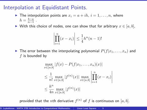
Interpolation at Equidistant Points.I The interpolation points are xi = a+ ih, i = 1, . . . , n, whereh = b−a

n−1 .

I With this choice of nodes, one can show that for arbitrary x ∈ [a, b],∣∣∣∣∣n∏

i=1

(x− xi)

∣∣∣∣∣ ≤ 14hn(n− 1)!

I The error between the interpolating polynomial P (f |x1, . . . , xn) andf is bounded by

maxx∈[a,b]

|f(x)− P (f |x1, . . . , xn)(x)|

≤ 1n!

maxx∈[a,b]


∣∣∣∣∣n∏

i=1

(x− xi)

∣∣∣∣∣≤ hn

4nmax

x∈[a,b]|f (n)(x)|

provided that the nth derivative f (n) of f is continuous on [a, b].


Interpolation at Chebyshev Points.

I Is there a choice x∗1, x∗2, . . . , x

∗n of nodes such that

maxx∈[a,b]

∣∣∣∣∣n∏

i=1

(x− x∗i )

∣∣∣∣∣is minimal?

I This leads to the minmax, or Chebyshev approximation problem

minx1,...,xn

maxx∈[a,b]

∣∣∣∣∣n∏

i=1

(x− x∗i )

∣∣∣∣∣ .


Interpolation at Chebyshev Points.

I The solution x∗1, . . . , x∗n of this problem are the socalled Chebyshev

points

x∗i =12

(a+ b) +12

(b− a) cos(

(2i− 1)π2n

), i = 1, . . . , n,

maxx∈[a,b]

∣∣∣∣∣n∏

i=1

(x− x∗i )

∣∣∣∣∣ ≤ 21−2n(b− a)n.

I Error between the interpolating polynomial P (f |x∗1, . . . , x∗n) and f :

maxx∈[a,b]

|f(x)−P (f |x∗1, . . . , x∗n)(x)| ≤ 21−2n(b− a)n

n!max

x∈[a,b]|f (n)(x)|,

provided that the nth derivative f (n) of f is continuous on [a, b].


Interpolation at Chebyshev Points.ExampleThe polynomial

∏ni=1(x− xi) with 10 equidistant points and 10

Chebychev points on [−1, 1].


Polynomial Interpolation.I Given data

x1 x2 · · · xn

f1 f2 · · · fn

(think of fi = f(xi)) we want to compute a polynomial pn−1 ofdegree at most n− 1 such that

pn−1(xi) = fi, i = 1, . . . , n.

I If xi 6= xj for i 6= j, there exists a unique interpolation polynomial.

I The larger n, the interpolation polynomial tends to become moreoscillatory.

I Let x1, x2, . . . , xn be unequal points. If f is n times differentiable,then for each x̄ there exists ξ(x̄) in the smallest interval containingthe points x1, x2, . . . , xn, x̄ such that

f(x̄)− P (f |x1, x2, . . . , xn)(x̄) =1n!

n∏j=1

(x̄− xj)

f (n)(ξ(x̄)).


Spline Interpolation.

I We do not use polynomials globally, but locally.

I Subdivide the interval [a, b] such that

a = x0 < x1 < · · · < xn = b.

Approximate the function f by a piecewise polynomial S such thatI on each subinterval [xi, xi+1] the function S is a polynomial Si of

degree k,I Si(xi) = f(xi) and Si(xi+1) = f(xi+1), i = 0, . . . , n− 1 (S

interpolates f at x0, . . . , xn),I

S(l)i−1(xi) = S

(l)i (xi), i = 1, . . . , n− 1, l = 1, . . . , k − 1

(the derivatives up to order k − 1 of S are continuous atx1, . . . , xn−1).

The function S is called a spline of degree k.

I We consider linear splines (k = 1) and cubic splines (k = 3).


Linear Splines.I Let a = x0 < x1 < · · · < xn = b be a partition of [a, b].I We want to approximate f by piecewise linear polynomials.I On each subinterval [xi, xi+1], i = 0, 1, . . . , n− 1, we consider the

linear polynomials

Si(x) = ai + bi(x− xi).

I The linear spline S satisfies the following properties:1. S(x) = Si(x) = ai + bi(x− xi), x ∈ [xi, xi+1] for i = 0, . . . , n− 1,2. S(xi) = f(xi) for i = 0, . . . , n,3. Si(xi+1) = Si+1(xi+1) for i = 0, . . . , n− 2,

I The conditions (1-3) uniquely determine the linear functionsSi(x) = ai + bi(x− xi). If we consider the ith subinterval [xi, xi+1],then ai, bi must satisfy

f(xi) = S(xi) = Si(xi) = ai + bi(xi − xi), and

f(xi+1) = Si+1(xi+1) = Si(xi+1) = ai + bi(xi+1 − xi).

This is a 2× 2 system for the unknowns ai, bi. Its solution is givenby

ai = f(xi), bi = (f(xi+1)− f(xi))/(xi+1 − xi).


MATLAB’s interp1.

MATLAB has a build-in function called interp1 that do 1−D datainterpolation.

Syntax:

yi = interp1(x,Y,xi)yi = interp1(Y,xi)yi = interp1(x,Y,xi,method)yi = interp1(x,Y,xi,method,’extrap’)yi = interp1(x,Y,xi,method,extrapval)pp = interp1(x,Y,method,’pp’)


MATLAB’s interp1.

yi = interp1(x,Y,xi)

interpolates to find yi, the values of the underlying function Y at thepoints in the vector or array xi. x must be a vector. Y can be a scalar, avector, or an array of any dimension, subject to the some conditions.To find out more, type

help interp1


MATLAB’s interp1.

ExampleConsider,

>> x = linspace(0,1,10);>> y = sin(x);

Thus we entered 10 uniform points of the sine function on the interval[0, 1]. Let’s say we want to approximate the value at π/6 by linearinterpolation. This can be done by

>> interp1(x,y,pi/6)

and give the answer

ans = 0.4994

which is rather crude since the exact answer is sin (π/6) = 0.5.


Cubic Splines.

I Let a = x0 < x1 < · · · < xn = b be a partition of [a, b].I On each subinterval [xi, xi+1], i = 0, 1, . . . , n− 1, we consider the

cubic polynomial Si(x) = ai + bi(x−xi) + ci(x−xi)2 + di(x−xi)3.I The cubic spline S satisfies the following properties:

1. S(x) = Si(x), x ∈ [xi, xi+1] for i = 0, . . . , n− 1,2. S(xi) = f(xi) for i = 0, . . . , n,3. Si(xi+1) = Si+1(xi+1) for i = 0, . . . , n− 2,4. S′i(xi+1) = S′i+1(xi+1) for i = 0, . . . , n− 2,5. S′′i (xi+1) = S′′i+1(xi+1) for i = 0, . . . , n− 2,

I To determine S we have to determine 4n parameters

ai, bi, ci, di, i = 0, . . . , n− 1.

I Equations (2-5) impose(n+ 1) + (n− 1) + (n− 1) + (n− 1) = 4n− 2 conditions on S.Therefore we need two additional conditions on S to specify theparameters uniquely.


Cubic Splines.

I The two conditions are either

S′′(x0) = S′′(xn) = 0 (natural or free boundary), (1)

or

S′(x0) = f ′(x0), S′(xn) = f ′(xn) (clamped boundary), (2)

or

S(i)(x0) = S(i)(xn), i = 0, 1, 2 (periodic spline). (3)

I A function S satisfying (1) is called a natural cubic spline,a function S satisfying (2) is called a clamped cubic spline, anda function S satisfying (3) is called a periodic cubic spline.


Convergence of Clamped Cubic Splines.

Theorem (Convergence of Clamped Cubic Splines)Let f ∈ C4([a, b]) and suppose that there exists K > 0 such that

hmax = maxi=0,...,n−1

hi ≤ K mini=0,...,n−1

hi,

where hi = xi+1 − xi.If S is the clamped cubic spline, i.e. spline satisfying (1), then there existconstants Ck such that

maxx∈[a,b]

|f (k)(x)− S(k)(x)| ≤ Ckh4−kmax max

x∈[a,b]|f (4)(x)|, k = 0, 1, 2,

and

|f (3)(x)− S(3)(x)| ≤ C3hmax maxx∈[a,b]

|f (4)(x)|, x ∈ ∪n−1i=0 (xi, xi+1).


MATLAB’s interp1 (cont).

The MATLAB’s function interp1 gives a choice the specify the methodof interpolation.

yi = interp1(x,Y,xi,method)

interpolates using alternative methods:

’nearest’ Nearest neighbor interpolation

’linear’ Linear interpolation (default)

’spline’ Cubic spline interpolation

’pchip’ Piecewise cubic Hermite interpolation

yi = interp1(x,Y,xi,method)


MATLAB’s interp1 (cont).

ExampleIn the previous example

>> x = linspace(0,1,10);>> y = sin(x);

Typing

>> interp1(x,y,pi/6,’spline’)

gives

ans = 0.499999897030974

which is much closer to 0.5 then 0.4994 from the linear interpolation.


MATLAB’s interp1 (cont). Example.Consider

>> x = 1:10;>> y = sin(x);plot(x,y)

produces a graph, that looks rather rough.


MATLAB’s interp1 (cont). Example.We can obtain a smoother graph by

>> xx = (1:10,100);>> yy = interp1(x,y,’spline’,xx);plot(xx,yy)


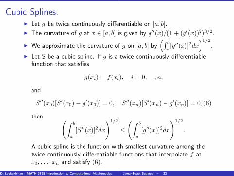
Cubic Splines.I Let g be twice continuously differentiable on [a, b].I The curvature of g at x ∈ [a, b] is given by g′′(x)/(1 + (g′(x))2)3/2.

I We approximate the curvature of g on [a, b] by(∫ b

a[g′′(x)]2dx

)1/2

.

I Let S be a cubic spline. If g is a twice continuously differentiablefunction that satisfies

g(xi) = f(xi), i = 0, , n,

and

S′′(x0)[S′(x0)− g′(x0)] = 0, S′′(xn)[S′(xn)− g′(xn)] = 0, (6)

then (∫ b

a

[S′′(x)]2dx

)1/2

≤

(∫ b

a

[g′′(x)]2dx

)1/2

.

A cubic spline is the function with smallest curvature among thetwice continuously differentiable functions that interpolate f atx0, . . . , xn and satisfy (6).


math 3795 lecture 15. polynomial interpolation. splines.leykekhman/courses/... · math 3795 lecture...

Documents