math 2210q applied linear algebra, fall 2016parzygnat/math2210f16/notes/2210qfall2016no… · math...

MATH 2210Q Applied Linear Algebra, Fall 2016

Arthur J. Parzygnat

These are my personal notes. This is not a substitute for Lay’s book, which shall henceforth

be referred to as [Lay]. You will not be responsible for any Remarks in these notes. However,

everything else, including what is in [Lay] (even if it’s not here), is fair game for homework, quizzes,

and exams. At the end of each lecture, I provide a list of homework problems that should be done

after that lecture. These homework problems will be collected every Tuesday! I also provide

additional exercises which I believe are good to know. You should also browse other books and do

other problems as well to get better at writing proofs and understanding the material.

Notes in light red are for the reader.

Notes in light green are reminders for me.

When a word or phrase is underlined, that typically means the definition of this word or phrase is

being given.

Contents

1 August 30 3

2 September 1 9

3 September 6 15

4 September 8 20

5 September 13 26

6 September 15 32

7 September 20 36

8 September 22 42

9 September 27 47

10 September 29 52

11 October 4 57

1

12 October 6 58

13 October 11 59

14 October 13 64

15 October 18 66

16 October 20 70

17 October 25 73

18 October 27 79

19 November 1 85

20 November 3 90

21 November 8 94

22 November 10 95

23 November 15 96

24 November 17 103

25 November 29 110

26 December 1 116

27 December 6 123

28 December 8 124

2

1 August 30

Hand out short questionnaire. Give them 5 minutes.

Linear algebra is the study of systems of linear equations of (in this course) a finite number of

variables. These are equations of the form

a11x1 + a12x2 + · · ·+ a1nxn = b1

a21x1 + a22x2 + · · ·+ a2nxn = b2

...

am1x1 + am2x2 + · · ·+ amnxn = bm,

(1.1)

where the aij are typically known constants (often real numbers), the bi are also known values,

and the xj are the variables which we would like to solve for.

Keep the above general form on the board throughout lecture.

It helps to start off immediately with some examples. We will slowly develop a more formal

and rigorous approach to linear algebra as the semester progresses. But for now, in the words of

Richard Feynman,1 “Shut up and calculate!”

Problem 1.2. [Exercise 33 in [Lay]] The temperature on the boundary of a cross section of a

metal beam is fixed and known but is unknown in the intermediate points on the interior

10

10

20

T1

T4

30

20

T2

T3

30

40

40(1.3)

Assume the temperature at these intermediate points equals the average of the temperature at

the nearest neighboring points.2 Write a system of linear equations to describe the temperatures

T1, T2, T3, and T4.

Answer. The system of equations is given by

T1 =1

4(10 + 20 + T2 + T4)

T2 =1

4(T1 + 20 + 40 + T3)

T3 =1

4(T4 + T2 + 40 + 30)

T4 =1

4(10 + T1 + T3 + 30)

(1.4)

1Wiki https://en.wikipedia.org/wiki/Copenhagen_interpretation suggests this phrase might actually be

due to David Mermin, another prominent physicist.2This is true to a good approximation and is in fact how approximation techniques can be used to solve problems

like this though the mesh will usually be much finer, and the boundary might not look so nice.

3

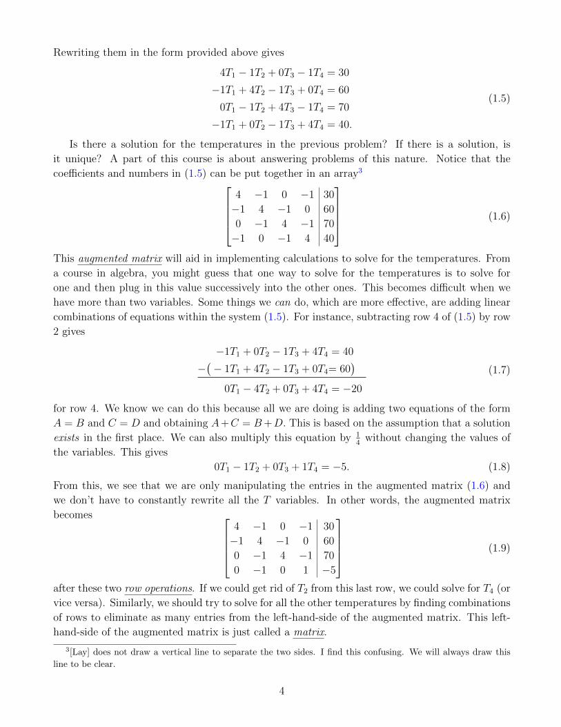
https://en.wikipedia.org/wiki/Copenhagen_interpretation

Rewriting them in the form provided above gives

4T1 − 1T2 + 0T3 − 1T4 = 30

−1T1 + 4T2 − 1T3 + 0T4 = 60

0T1 − 1T2 + 4T3 − 1T4 = 70

−1T1 + 0T2 − 1T3 + 4T4 = 40.

(1.5)

Is there a solution for the temperatures in the previous problem? If there is a solution, is

it unique? A part of this course is about answering problems of this nature. Notice that the

coefficients and numbers in (1.5) can be put together in an array34 −1 0 −1 30

−1 4 −1 0 60

0 −1 4 −1 70

−1 0 −1 4 40

(1.6)

This augmented matrix will aid in implementing calculations to solve for the temperatures. From

a course in algebra, you might guess that one way to solve for the temperatures is to solve for

one and then plug in this value successively into the other ones. This becomes difficult when we

have more than two variables. Some things we can do, which are more effective, are adding linear

combinations of equations within the system (1.5). For instance, subtracting row 4 of (1.5) by row

2 gives

−1T1 + 0T2 − 1T3 + 4T4 = 40

−(− 1T1 + 4T2 − 1T3 + 0T4= 60

)0T1 − 4T2 + 0T3 + 4T4 = −20

(1.7)

for row 4. We know we can do this because all we are doing is adding two equations of the form

A = B and C = D and obtaining A+C = B+D. This is based on the assumption that a solution

exists in the first place. We can also multiply this equation by 14

without changing the values of

the variables. This gives

0T1 − 1T2 + 0T3 + 1T4 = −5. (1.8)

From this, we see that we are only manipulating the entries in the augmented matrix (1.6) and

we don’t have to constantly rewrite all the T variables. In other words, the augmented matrix

becomes 4 −1 0 −1 30

−1 4 −1 0 60

0 −1 4 −1 70

0 −1 0 1 −5

(1.9)

after these two row operations. If we could get rid of T2 from this last row, we could solve for T4 (or

vice versa). Similarly, we should try to solve for all the other temperatures by finding combinations

of rows to eliminate as many entries from the left-hand-side of the augmented matrix. This left-

hand-side of the augmented matrix is just called a matrix.

3[Lay] does not draw a vertical line to separate the two sides. I find this confusing. We will always draw this

line to be clear.

4

Problem 1.10 (Exercise 34 in [Lay]). Solve the system of linear equations in (1.5).

Answer. Let’s begin by adding 4 of row 2 to row 10 15 −4 −1 270

−1 4 −1 0 60

0 −1 4 −1 70

0 −1 0 1 −5

. (1.11)

Add 15 of row 4 to row 1 0 0 −4 14 195

−1 4 −1 0 60

0 −1 4 −1 70

0 −1 0 1 −5

(1.12)

Subtract row 4 from row 3 0 0 −4 14 195

−1 4 −1 0 60

0 0 4 −2 75

0 −1 0 1 −5

(1.13)

Add row 3 to row 1 0 0 0 12 270

−1 4 −1 0 60

0 0 4 −2 75

0 −1 0 1 −5

(1.14)

Divide row 1 by 6 0 0 0 2 45

−1 4 −1 0 60

0 0 4 −2 75

0 −1 0 1 −5

(1.15)

Add row 1 to row 3 and subtract half of row 1 from row 40 0 0 2 45

−1 4 −1 0 60

0 0 4 0 120

0 −1 0 0 −27.5

(1.16)

Add 4 of row 4 to row 2 and divide row 3 by 40 0 0 2 45

−1 0 −1 0 −50

0 0 1 0 30

0 −1 0 0 −27.5

(1.17)

Add row 3 to row 2 0 0 0 2 45

−1 0 0 0 −20

0 0 1 0 30

0 −1 0 0 −27.5

(1.18)

5

Multiply rows 2 and 4 by −1 and divide row 1 by 20 0 0 1 22.5

1 0 0 0 20

0 0 1 0 30

0 1 0 0 27.5

(1.19)

In other words, we have found a solution

T1 = 20

T2 = 27.5

T3 = 30

T4 = 22.5

(1.20)

Because it helps to visualize this the same way, we can permute the rows and still have the same

equations describing our problem 1 0 0 0 20

0 1 0 0 27.5

0 0 1 0 30

0 0 0 1 22.5

(1.21)

This is another example of a row operation.

You should check these solutions by plugging them back into the original linear system (1.5).

In total, we have used three row operations to help us solve linear systems:

(a) scaling rows,

(b) adding rows, and

(c) permuting rows.

In this situation, we were lucky and a solution existed and was unique. Sometimes, a solution

need not exist or if one exists, it might not be unique.

Example 1.22. Let

2x+ 3y = 5

4x+ 6y = −2(1.23)

be two linear equations in the variables x and y. There is no solution to this system. If there were

a solution, then dividing the second line by 2 would give 5 = −1, which is impossible.4 This can

also be seen by plotting these two equations in the plane as in Figure 1. These two lines do not

intersect.Go to Mathematica and draw the plot.

4This is an example of a proof by contradiction.

6

-2 -1 1 2

-1

1

2

3

2x+ 3y = 5

4x+ 6y = −2

Figure 1: A plot of the equations 2x+ 3y = 5 and 4x+ 6y = −2.

Example 1.24. Consider the linear system given by

−x− y + z = −2

−2x+ y + z = 1(1.25)

These two equations are plotted in Figure 2.

−x− y + z = −2

−2x+ y + z = 1

Figure 2: A plot of the equations −x− y + z = −2 and −2x+ y + z = 1.

Go to Mathematica and draw the plot.

It is clear from this picture that there are solutions, in fact a lines worth of solutions instead

of a unique one (the intersection of the two planes is the set of solutions). How can we describe

this line explicitly? Looking at (1.25), we can add the two equations to get5

− 3x+ 2z = −1 ⇐⇒ z =1

2(3x− 1) (1.26)

5The ⇐⇒ symbol means “if and only if,” which in this context means that the two equations are equivalent.

7

We can also subtract the second equation from the first to get

x− 2y = −3 ⇐⇒ y =1

2(3 + x). (1.27)

Hence, the set of points given by (x,

1

2(3 + x),

1

2(3x− 1)

)(1.28)

as x varies over real numbers, are all solutions of (1.25). We can plot this in Figure 3.

Figure 3: A plot of the equations −x − y + z = −2 and −2x + y + z = 1 together with the

intersection shown in red and given parametrically as x 7→(x, 1

2(3 + x), 1

2(3x− 1)

).

Go to Mathematica and draw the plot.

In the example 1.22, the set of solutions is empty. Such a system is said to be inconsistent.

A linear system where the solution set is non-empty is said to be consistent. In example 1.24,

there is more than one solution. The solution set of a linear system (1.1) is the collection of all

(x1, x2, . . . , xn) that satisfy (1.1). In problem 1.2, there is only one element in the solution set.

Occasionally, two arbitrary linear systems may have the same set of solutions. Two linear systems

of equations that have the same set of solutions are said to be equivalent. Hence, the two linear

systems of equations given in (1.5) and (1.21) are equivalent.

Homework (Due: Tuesday September 6). Exercises 2, 3, 12, 14, 16, 17, 18, 27, and 28 in Section

1.1 of [Lay]. Please show all your work, step by step! Do not use calculators or computer programs

to solve any problems!

8

2 September 1

As we do more problems, we get familiar with faster methods of solving systems of linear equations.

We start with another problem from circuits with batteries and resistors.

Problem 2.1. Consider a circuit of the following form

6 V2 V

4 Ohm

1 Ohm

3 Ohm

Here the jagged lines represent resistors and the two parallel lines, with one shorter than the

other, represent batteries with the positive terminal on the longer side. The units of resistance

are Ohms and the units for voltage are Volts. Find the current (in units of Amperes) across each

resister along with the direction of current flow.

Answer. Kirchhoff’s rule says that the the voltage difference across any closed loop in a circuit

with resistors and batteries is always zero. Across a resistor, the voltage drop is the current times

the resistance. Across a battery from the negative to positive terminal, there is a voltage increase

given by the voltage of the battery. There is also the rule that says current is always conserved,

meaning that at a junction, current in equals current out. Knowing this, we label the currents in

the wires by I1, I2, and I3 as follows.

6 V2 V

4 Ohm

I1−−−−→

I2−−−−→

1 Ohm I3

−−−−→

2 Ohm

Conservation of current gives

I1 = I2 + I3. (2.2)

Kirchhoff’s rule for the left loop in the circuit gives

2− 4I1 − 1I3 = 0 (2.3)

and for the right loop gives

− 6− 2I2 + 1I3 = 0. (2.4)

These are three equations in three unknowns.

If you were lost up until this point, that’s fine. You can start by assuming the following form

for the linear system of equations.

9

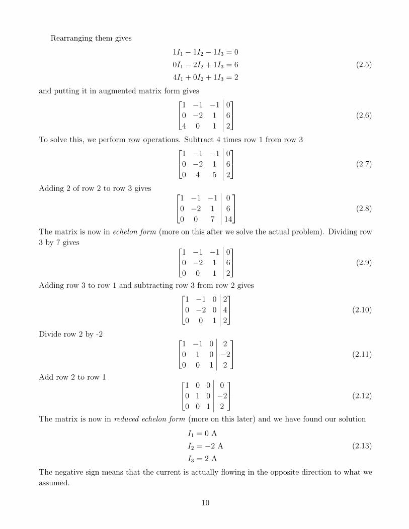
Rearranging them gives

1I1 − 1I2 − 1I3 = 0

0I1 − 2I2 + 1I3 = 6

4I1 + 0I2 + 1I3 = 2

(2.5)

and putting it in augmented matrix form gives1 −1 −1 0

0 −2 1 6

4 0 1 2

(2.6)

To solve this, we perform row operations. Subtract 4 times row 1 from row 31 −1 −1 0

0 −2 1 6

0 4 5 2

(2.7)

Adding 2 of row 2 to row 3 gives 1 −1 −1 0

0 −2 1 6

0 0 7 14

(2.8)

The matrix is now in echelon form (more on this after we solve the actual problem). Dividing row

3 by 7 gives 1 −1 −1 0

0 −2 1 6

0 0 1 2

(2.9)

Adding row 3 to row 1 and subtracting row 3 from row 2 gives1 −1 0 2

0 −2 0 4

0 0 1 2

(2.10)

Divide row 2 by -2 1 −1 0 2

0 1 0 −2

0 0 1 2

(2.11)

Add row 2 to row 1 1 0 0 0

0 1 0 −2

0 0 1 2

(2.12)

The matrix is now in reduced echelon form (more on this later) and we have found our solution

I1 = 0 A

I2 = −2 A

I3 = 2 A

(2.13)

The negative sign means that the current is actually flowing in the opposite direction to what we

assumed.

10

You should check these solutions by plugging them back into the original linear system.

Given a linear system of equations as in (1.1), which is written as an augmented matrix asa11 a12 · · · a1n b1

a21 a22 · · · a2n b2

......

. . ....

...

am1 am2 · · · amn bm

, (2.14)

an echelon form of such an augmented matrix is an equivalent augmented matrix whose matrix

components (to the left of the vertical line) satisfy the following conditions.

(a) All nonzero rows are above any rows containing only zeros.

(b) The first entry (from the left), also known as a pivot, of any nonzero row is always to the right

of the first nonzero entry of the row above it.

(c) All entries in the column below a pivot are zeros.

The column corresponding to a pivot is called a pivot column.

Draw a few on the board.

For the student reading these notes, look in [Lay].

A matrix is in reduced echelon form if in addition the following hold.

(d) All pivots are 1.

(e) The pivots are the only nonzero entries in the corresponding pivot columns.

Draw a few reduced row echelon form matrices on the board.

For the student reading these notes, look in [Lay].

It is a fact that the reduced row echelon form of a matrix is always unique provided that the

linear system corresponding to it is consistent. Furthermore, a linear system is consistent if and

only if an echelon form of the augmented matrix does not contain any rows of the form[0 · · · 0 b

]with b nonzero (2.15)

In our earlier examples of temperature on a rod from lecture 1 and currents in a circuit from

this lecture, the arrays of numbers given byT1

T2

T3

T4

&

I1

I2

I3

(2.16)

11

are examples of vectors in R4 and R3, respectively. Here R is the set of real numbers and Rn is

the set of n-tuples of real numbers where n is a positive integer being one of 1, 2, 3, 4, . . . . Given

two vectors in Rn, a1

...

an

&

b1

...

bn

(2.17)

we can take their sum defined by a1

...

an

+

b1

...

bn

:=

a1 + b1

...

an + bn

. (2.18)

We can also scale each vector by any number c in R by

c

a1

...

an

:=

ca1

...

can

. (2.19)

The above descriptions of vectors are algebraic and we’ve illustrated their algebraic structures

(addition and scaling). Vectors can also be visualized when n = 1, 2, 3.

Draw a few vectors in R2 and R3. Note that the vectors are not actually the arrows drawn but

the endpoints of these arrows. The arrows merely help for visualizations of operations such as

addition of vectors.

We will often write vectors with an arrow over them as in ~a and ~b when n is understood. Let

S := ~v1, . . . , ~vm be a set of m vectors in Rn. The span of S is the set of all vectors of the form6

m∑i=1

ai~vi ≡ a1~v1 + · · · am~vm, (2.20)

where the ai can be any real number. For a fixed set of ai, the right-hand-side of (2.20) is called

a linear combination of the vectors ~vi.

In set-theoretic notation, we would write this as

span(S) :=

m∑i=1

ai~vi ∈ Rn : a1, . . . , am ∈ R

. (2.21)

The span of vectors in R2 and R3 can be visualized quite nicely.

6Please do not confuse the notation ~vi with the components of the vector ~vi. It can be confusing with these

indices, but to be very clear, we could write the components of the vector ~vi as(vi)1...

(vi)n

.

12

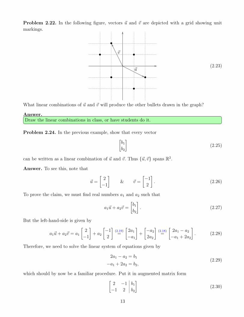
Problem 2.22. In the following figure, vectors ~u and ~v are depicted with a grid showing unit

markings.

•

•

••

•

•

OO

//~u

''

~v

WW

(2.23)

What linear combinations of ~u and ~v will produce the other bullets drawn in the graph?

Answer.Draw the linear combinations in class, or have students do it.

Problem 2.24. In the previous example, show that every vector[b1

b2

](2.25)

can be written as a linear combination of ~u and ~v. Thus ~u,~v spans R2.

Answer. To see this, note that

~u =

[2

−1

]& ~v =

[−1

2

]. (2.26)

To prove the claim, we must find real numbers a1 and a2 such that

a1~u+ a2~v =

[b1

b2

]. (2.27)

But the left-hand-side is given by

a1~u+ a2~v = a1

[2

−1

]+ a2

[−1

2

](2.19)=

[2a1

−a1

]+

[−a2

2a2

](2.18)=

[2a1 − a2

−a1 + 2a2

]. (2.28)

Therefore, we need to solve the linear system of equations given by

2a1 − a2 = b1

−a1 + 2a2 = b2,(2.29)

which should by now be a familiar procedure. Put it in augmented matrix form[2 −1 b1

−1 2 b2

](2.30)

13

Permute the first and second rows [−1 2 b2

2 −1 b1

](2.31)

Add two of row 1 to row 2 to get [−1 2 b2

0 3 b1 + 2b2

](2.32)

This is now in echelon form. Multiply row 1 by −1 and divide row 2 by 3[1 −2 −b2

0 1 13(b1 + 2b2)

](2.33)

Add 2 of row 2 to row 1 [1 0 −b2 + 2

3(b1 + 2b2)

0 1 13(b1 + 2b2)

](2.34)

which is equal to [1 0 1

3(2b1 + b2)

0 1 13(b1 + 2b2)

](2.35)

which says that [b1

b2

]=

(2b1 + b2

3

)~u+

(b1 + 2b2

3

)~v. (2.36)

Homework (Due: Tuesday September 6). Exercises 8, 12, 13, 16, 24, 26, and 29 in Section 1.2

of [Lay]. Exercises 3, 4, 7, 8, 12, 18, 25, 26, and 32 in Section 1.3 of [Lay]. Please show all your

work, step by step! Do not use calculators or computer programs to solve any problems!

14

3 September 6

HW #01 is due at the beginning of class!

An augmented matrix of the form (2.14) corresponding to a linear system (1.1) with variables

x1, . . . , xn, can be expressed as

A~x = ~b, (3.1)

where the notation A~x stands for the vector 7a11 a12 · · · a1n

a21 a22 · · · a2n

......

...

am1 am2 · · · amn

x1

x2

...

xn

:=

a11x1 + a12x2 + · · ·+ a1nxna21x1 + a22x2 + · · ·+ a2nxn

...

am1x1 + am2x2 + · · ·+ amnxn

(3.2)

in Rm (yes, that’s an m, not an n). Therefore, an m× n matrix acts on a vector in Rn to produce

a vector in Rm. We will discuss this more next week. Warning: we do not provide a definition

for an m× n matrix acting on a vector in Rk with k 6= n.

Give a simple example in class!

This is a way of consolidating the augmented matrix and A is precisely the matrix corresponding

to the linear system. One can also express the matrix A as a row of column vectors

A =[~a1 ~a2 · · · ~an

](3.3)

where the i-th component of the j-th vector ~aj is given by

(~aj)i = aij. (3.4)

In this case, ~b is explicitly expressed as a linear combination of the vectors ~a1, . . . ,~an via

~b = x1~a1 + · · ·+ xn~an. (3.5)

Therefore, solving for the variables x1, . . . , xn for the linear system (1.1) is equivalent to finding

coefficients x1, . . . , xn that satisfy (3.5). (3.5) is called a matrix equation. Here A is an m × n

matrix.8

Thus, there are three equivalent ways to express a linear system.

(a) m linear equations in n variables (1.1).

(b) An augmented matrix (2.14).

(c) A matrix equation A~x = ~b as in (3.2).

The above observations also lead to the following.

7The vector on the right-hand-side is a definition of the notation on the left-hand-side. Don’t be confused by

the fact that there are a lot of terms inside each component of the vector on the right-hand-side of (3.2)—it is not

an m× n matrix!8Here m× n stands for m rows and n columns.

15

Theorem 3.6. Let A be a fixed m × n matrix. The following statements are equivalent (which

means that any one implies the other and vice versa).

(a) For every vector ~b in Rm, the solution set of the equation A~x = ~b, meaning the set of all ~x

satisfying this equation, is nonempty.

(b) Every vector ~b in Rm can be written as a linear combination of the columns of A, viewed as

vectors in Rm, i.e. the columns of A span Rm.

(c) A has a pivot position in every row.

Proof. Let’s just check part of the equivalence between (a) and (b) by showing that (b) implies

(a). Suppose that a vector ~b can be written as a linear combination

~b = x1~a1 + · · ·+ xn~an, (3.7)

where the x1, . . . , xn are some coefficients. Rewriting this using column vector notation gives b1

...

bm

= x1

(a1)1

...

(a1)m

+ · · ·+ xn

(an)1

...

(an)m

(3.8)

We can set our notation and write

(aj)i ≡ aij. (3.9)

Then, writing out this equation of vectors gives b1

...

bm

=

x1a11 + · · ·+ xna1n

...

x1am1 + · · ·+ xnamn

(3.10)

by the rules about scaling and adding vectors from last lecture. The resulting equation is exactly

the linear system corresponding to A~x = ~b. Hence, the x’s from the linear combination in (3.7)

give a solution of the matrix equation A~x = ~b.

Do a simple example in class by writing out 3 vectors ~a1,~a2,~a3 and some other vector ~b and

writing out the system to figure out if ~b is in the span of ~a1,~a2,~a3. If the resulting linear sys-

tem is consistent, a solution exists and ~b is in the span of ~a1,~a2,~a3. If it is inconsistent, no

solution exists and ~b is not in the span of ~a1,~a2,~a3.

Theorem 3.11. Let A be an m×n matrix, let ~x and ~y be two vectors in Rn, and let c be any real

number. Then

A(~x+ ~y) = A~x+ A~y & A(c~x) = cA~x. (3.12)

Exercise 3.13. Prove this! To do this, write out an arbitrary A matrix with entries as in (3.2)

along with two vectors ~x and ~y and simply work out both sides of the equation using the rule in

(3.2).

16

Give an example instead of proving the theorem.

Problem 3.14 (Exercise 8 in Section 1.6 of [Lay]). Consider a chemical reaction that turns

limestone CaCO3 and acid H3O into water H2O, calcium Ca, and carbon dioxide CO2. In a chemical

reaction, all elements must be accounted for. Find the appropriate ratios of these compounds and

elements needed for this reaction to occur without other waste products.

Answer. Introduce variables x1, x2, x3, x4 and x5 for the coefficients of limestone, acid, water, cal-

cium, and carbon dioxide, respectively. The elements appearing in these compounds and elements

are H, O, C, and Ca. We can therefore write the compounds as a vector in these variables (in this

order). For example, limestone, CaCO3, is 0

3

1

1

← H

← O

← C

← Ca

(3.15)

since it is composed of zero hydrogen atoms, three oxygen atoms, one carbon atom, and one

calcium atom. Thus, the linear system we need to solve is given by

x1CaCO3 + x2H3O = x3H2O + x4Ca + x5CO2

x1

0

3

1

1

+ x2

3

1

0

0

= x3

2

1

0

0

+ x4

0

0

0

1

+ x5

0

2

1

0

(3.16)

The associated augmented matrix is0 3 −2 0 0 0

3 1 −1 0 −2 0

1 0 0 0 −1 0

1 0 0 −1 0 0

(3.17)

and the associated matrix equation is given by

A~x = ~b, (3.18)

where A is the left-hand-side of the augmented matrix and ~b = ~0, the zero vector. Subtract row 4

from row 3 and subtract 3 of row 4 from row 20 3 −2 0 0 0

0 1 −1 3 −2 0

0 0 0 1 −1 0

1 0 0 −1 0 0

(3.19)

Subtract 3 of row 2 from row 1 0 0 1 −9 6 0

0 1 −1 3 −2 0

0 0 0 1 −1 0

1 0 0 −1 0 0

(3.20)

17

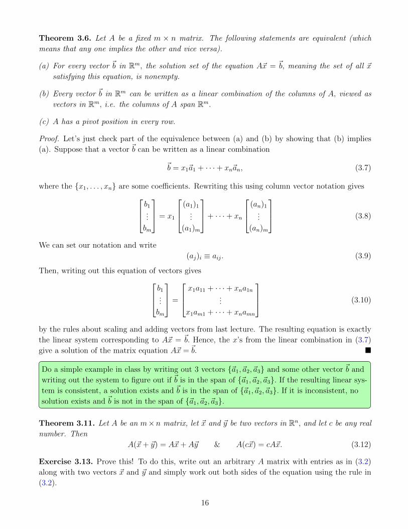
Permute the rows so that the augmented matrix is in echelon form1 0 0 −1 0 0

0 1 −1 3 −2 0

0 0 1 −9 6 0

0 0 0 1 −1 0

(3.21)

Add row 4 to row 1 and add row 3 to row 21 0 0 0 −1 0

0 1 0 −6 4 0

0 0 1 −9 6 0

0 0 0 1 −1 0

(3.22)

Add 9 of row 4 to row 3 and add 6 of row 4 to row 21 0 0 0 −1 0

0 1 0 0 −2 0

0 0 1 0 −3 0

0 0 0 1 −1 0

(3.23)

Now the augmented matrix is in reduced echelon form. Notice that although solutions exist, they

are not unique! We saw this happening in example 1.24 back in lecture 1. Let us write the

concentrations in terms of x5, the concentration of calcium.

x1 = x5, x2 = 2x5, x3 = 3x5, & x4 = x5. (3.24)

Thus, the resulting reaction is given by

x5CaCO3 + 2x5H3O→ 3x5H2O + x5Ca + x5CO2 (3.25)

It is common to set the smallest quantity to 1 so that this becomes

CaCO3 + 2H3O→ 3H2O + Ca + CO2. (3.26)

Nevertheless, we do not have to do this, and a proper way to express the solution is in terms of

the concentration of calcium (for instance) asx1

x2

x3

x4

x5

= x5

1

2

3

1

1

. (3.27)

We did not have to choose calcium as the free variable. Any of the other elements would have

been as good of a choice as any other, but in some instances, the resulting coefficients might be

fractions.

18

The previous example leads us to the notion of homogeneous linear systems. A linear system

A~x = ~b is said to be homogeneous if ~b = ~0. Note that a homogeneous linear system always has at

least one solution, namely ~x = ~0, which is called the trivial solution. We have also noticed in the

example that there is a free variable in the solution. This is a generic phenomena:

Theorem 3.28. The homogeneous equation A~x = ~0 has a nontrivial solution if and only if the

corresponding system of linear equations has a free variable.

In (3.27), the solution of the homogeneous equation was written in the form

~x = ~p+ t~v (3.29)

where in that example ~p was ~0, t was x5, and ~v was the vector1

2

3

1

1

. (3.30)

This form of the solution of a linear equation is in parametric form because its value depends on an

additional unspecified parameter, which in this case is t. In other words, all solutions are valid as

t varies over the real numbers. For a homogeneous equation, ~p is always ~0 (because then ~0 would

not be a solution, contradicting A~x = ~0). In fact, there could be more than one such parameter

involved.

Theorem 3.31. Suppose that the linear system described by A~x = ~b is consistent and let ~x = ~p be

a solution. Then the solution set of A~x = ~b is the set of all vectors of the form ~p + ~u where ~u is

any solution of the homogeneous equation A~x = ~0.

This says that the solution set of a consistent linear system A~x = ~b can be expressed as

~x = ~p+ t1~u1 + · · ·+ tk~uk, (3.32)

where ~p is one solution of A~x = ~b, k is a positive integer, t1, . . . , tk are the parameters (real

numbers), and the set ~u1, . . . , ~uk spans the solution set of A~x = ~0. A linear combination of

solutions to A~x = ~0 is a solution as well. This problem will be addressed in your homework! You

may want to use Theorem 3.11 to prove this last statement.

Homework (Due: Tuesday September 13). Exercises 4, 7, 10, 25, 30, and 32 in Section 1.4 of

[Lay]. Exercises 2, 5, 15, 37, and 39 in Section 1.5 of [Lay]. Please show all your work, step by

step! Do not use calculators or computer programs to solve any problems!

19

4 September 8

Quiz (review of what we covered on Aug 30 and Sep 1) at the beginning of class!

Today is proof day! We will slowly begin more formal aspects of linear algebra.

Definition 4.1. A set of vectors ~u1, . . . , ~uk in Rn is linearly independent if the solution set of

the vector equation9

x1~u1 + · · ·+ xk~uk = ~0 (4.2)

consists of only the trivial solution. Otherwise, the set is said to be linearly dependent in which

case there exist some coefficients x1, . . . , xk not all of which are zero such that (4.2) holds.

Example 4.3. The vectors 1

−2

0

&

−3

6

0

(4.4)

are linearly dependent because −3

6

0

= −3

1

−2

0

(4.5)

so that

3

1

−2

0

+

−3

6

0

= 0. (4.6)

Example 4.7. The vectors [1

1

]&

[−1

1

](4.8)

are linearly independent for the following reason. Let x1 and x2 be two real numbers such that

x1

[1

1

]+ x2

[−1

1

]=

[0

0

]. (4.9)

This equation describes the system associated to the augmented matrix[1 −1 0

1 1 0

]. (4.10)

Subtracting row 1 from row 2 gives [1 −1 0

0 2 0

]. (4.11)

Dividing row 2 by 2 and then adding it to row 1 gives[1 0 0

0 1 0

]. (4.12)

The only solution to (4.9) is therefore x1 = 0 and x2 = 0. Thus, the two vectors in (4.8) are linearly

independent.

9Recall, the solution set is the set of all x1, . . . , xk satisfying (4.2).

20

Example 4.13. A set ~u1, ~u2 of two vectors in Rm is linearly dependent if and only if10 one can

be written as a scalar multiple of the other, i.e. there exists a real number c such that ~u1 = c~u2 or

c~u1 = ~u2.

This is going to be our first full proof. We will therefore try to guide you using footnotes so

that you know what is part of the proof and what is based on intuition. Instead of first teach-

ing you how to do proofs from scratch, we will go through several examples so that you see

what they are like first. This is like learning a new language. Before learning the grammar,

you want to first listen to people talking to get a feel for what the language sounds like. Then,

when you learn the alphabet, you want to read a few passages before you start constructing

sentences on your own.

Proof. First11 note that the associated vector equation is of the form

x1~u1 + x2~u2 = ~0, (4.14)

where12 x1 and x2 are coefficients, or upon rearranging

x1~u1 = −x2~u2. (4.15)

(⇒) If the set is linearly dependent, then x1 and x2 cannot both be zero.13 Without loss of

generality, suppose that x1 is nonzero.14 Then dividing both sides of (4.15) by x1 gives

~u1 = −x2

x1

~u2. (4.16)

Thus, setting c := −x2x1

proves the first claim15 (a similar argument can be made if x2 is nonzero).

(⇐) Conversely,16 suppose that there exists a real number c such that17 ~u1 = c~u2. Then

~u1 − c~u2 = ~0 (4.17)

showing that the set ~u1, ~u2 is linearly dependent since the coefficient in front of ~u1 is nonzero (it

is 1).18

At the end of a proof, you should always check your work!

Draw a few situations where a set of vectors is linearly dependent and independent first in R2

and then in R3.

10To prove a statement of the form “A if and only if B,” one must show that A implies B and B implies A. In a

proof, we often depict the former by (⇒) and the latter by (⇐).11Before proving anything, we just recall what the vector equation is to remind us of what we’ll need to refer to.12If you introduce notation in a proof, please say what it is every time!13What we have done so far is just state the definition of what it means for ~u1, ~u2 to be linearly dependent.

Stating these definitions to remind ourselves of what we know is a large part of the battle in constructing a proof.14We know from the definition that at least one of x1 or x2 is not zero but we do not know which one. It won’t

matter which one we pick in the end (some insight is required to notice this), so we may use the phrase “without

loss of generality” to cover all other possible cases.15Remember, we wanted to show that ~u1 is a scalar multiple of ~u2.16We say “conversely” when we want to prove an assertion in the opposite direction to the previously proven

assertion.17Remember, this is literally the latter assumption in the claim.18Recall the definition of what it means to be linearly dependent and confirm that you agree with the conclusion.

21

Example 4.18. Let

x :=

1

0

0

, y :=

0

1

0

, & z :=

0

0

1

(4.19)

be the three unit vectors in R3 (sometimes denoted by i, j, and k, respectively). In addition, let ~u

be any other vector in R3. Then the set x, y, z, ~u is linearly dependent because ~u can be written

as a linear combination of the three unit vectors. This is obvious because if we write

~u =

u1

u2

u3

(4.20)

then

~u = u1x+ u2y + u3z. (4.21)

Here’s a less trivial example.

Example 4.22. The vectors 1

0

1

,2

1

3

, &

−1

−2

−3

(4.23)

are linearly dependent. This is a little bit more difficult to see so let us try to solve it from scratch.

We must find x1, x2, and x3 such that

x1

1

0

1

+ x2

2

1

3

+ x3

−1

−2

−3

=

0

0

0

. (4.24)

This is exactly a matrix equation by Theorem (3.6). Hence, we have to solve the augmented matrix

system given by 1 2 −1 0

0 1 −2 0

1 3 −3 0

(4.25)

which after some row operations is equivalent to1 0 3 0

0 1 −2 0

0 0 0 0

. (4.26)

This has non-zero solutions. Setting x3 = −1 (we don’t have to do this—we can leave x3 as a free

variable, but I just want to show that we can write the last vector in terms of the first two) shows

that −1

−2

−3

= 3

1

0

1

− 2

2

1

3

. (4.27)

22

The previous examples hint at a more general situation.

Theorem 4.28. Let S := ~u1, . . . , ~uk be a set of vectors in Rn. S is linearly dependent if and

only if at least one vector from S can be written as a linear combination of the others.

The proof of Theorem 4.28 will be similar to the previous example. Why should we expect

this? Well, if k = 3, then we have ~u1, ~u2, ~u3 and we could imagine doing something very similar.

Think about this! If you’re not comfortable working with arbitrary k just yet, specialize to the

case k = 3 and try to mimic the previous proof. Then try k = 4. Do you see the pattern? Once

you’re ready, try the following.

Ask the students for suggestions!

If this is your first time proving things outside of geometry in highschool, study how these

proofs are written. Try to prove things on your own. Do not be discouraged if you are wrong.

Keep trying. A good book on learning how to think about proofs is How to Solve It by G.

Polya [1]. A course in discrete mathematics also helps. Practice, practice, practice!

Proof. The vector equation associated to S is

k∑j=1

xj~uj = ~0, (4.29)

where the xj are coefficients.

(⇒) If the set S is linearly dependent, then there exists19 a nonzero xi (for some i between 1 and

k). Therefore,

~ui =k∑j 6=i

(−xjxi

)~uj, (4.30)

where the sum is over all numbers j from 1 to k except i. Hence, the vector ~ui can be written as

a linear combination of the others.

(⇐) Conversely, suppose that there exists a vector ~ui from S that can be written as a linear

combination of the others, i.e.

~ui =k∑j 6=i

yj~uj, (4.31)

where the yj are real numbers.20 Rearranging gives

~ui −k∑j 6=i

xj~uj = 0, (4.32)

and we see that the coefficient in front of ~ui is nonzero (it is 1). Hence S is linearly dependent.

The following two theorems will give quick methods to figure out whether a given set of vectors

is linearly dependent.

19By definition of a linearly dependent set, at least one of the xi’s must be nonzero. This is phrased concisely by

the statement “there exists a nonzero xi...”.20We call our variables y to avoid potentially confusing them with the previous variables x.

23

Theorem 4.33. Let S := ~u1, . . . , ~uk be a set of vectors in Rn with k > n. Then S is linearly

dependent.

Proof. Recall, S is linearly dependent21 if there exist numbers x1, . . . , xk not all zero such that

k∑i=1

xi~ui = ~0. (4.34)

This equation can be expressed as a linear system

k∑i=1

xi(ui)1 = 0

...

k∑i=1

xi(ui)n = 0,

(4.35)

where22 (ui)j is the j-th component of the vector ~ui. In this linear system, there are k unknowns

given by the variables x1, . . . , xk and there are n equations. Because k > n, there are more

unknowns than equations, and hence there is at least one free variable.23 Let xp be one of these

free variables. Then the other xi’s might depend on xp so we may write xi(xp).24 Then by setting

xp = 1, we find

1~up +k∑i 6=p

xi(xp = 1)~ui = ~0 (4.36)

showing that S is linearly dependent (again since the coefficient in front of ~up is nonzero).

Warning! Using an example of S := ~u1, . . . , ~uk and showing that it is linearly dependent is not

a proof! We have to prove the claim for all potential cases. Nevertheless, an example helps to see

why the claim might be true in the first place.

Theorem 4.37. Let S := ~u1, . . . , ~uk be a set of vectors in Rn with at least one of the ~ui being

zero. Then S is linearly dependent.

Proof. Suppose ~ui = ~0. Then choose25 the coefficient of ~uj to be

xj :=

1 if j = i

0 otherwise(4.38)

21Again, it is always helpful to constantly remind yourself and the reader of definitions that are crucial to solving

the problem at hand. It is also helpful to use them to introduce notation that has not been introduced in the

statement of the claim (the theorem).22We have introduced some notation, so we should define it.23But wait, how do we know that a solution even exists? If a solution doesn’t exist, then our conclusion must

be false! Thankfully, by our earlier comments from the previous lecture, we know that every homogeneous linear

system has at least one solution, namely the trivial solution. Hence, the solution set is not empty.24This is read as “xi is a function of xp.”25To show that the set is linearly dependent, we have to find a set of coefficients, not all of which are zero, so

that their linear combination results in the zero vector. The coefficients that I’ve chosen here are not the only

coefficients that will work. You may choose have chosen others. All we have to do is exhibit the existence of one

such choice. We do not have to exhaust all posibilities.

24

Thenk∑j=1

xj~uj = 1~ui = 1(~0) = ~0 (4.39)

because any scalar multiple of the zero vector is the zero vector. Since not all of the coefficients

are zero (one of them is 1), S is linearly dependent.

Homework (Due: Tuesday September 13). Exercises 6, 8, 10, 14, 22, 34, 36, and 38 in Section 1.7

of [Lay]. Please note: For exercises 34, 36, and 38, if the statements are true, prove them! That’s

what “justification” means. You may (and are encouraged to) use any theorems we have done in

class! Please show all your work, step by step! Do not use calculators or computer programs to

solve any problems!

25

5 September 13


As we discussed last week, an m× n matrix A acts on a vector ~x in Rn and produces a vector~b in Rm as in

A~x = ~b. (5.1)

Furthermore, a matrix acting on vectors in Rn in this way satisfies the following two properties

A(~x+ ~y) = A~x+ A~y (5.2)

and

A(c~x) = cA~x (5.3)

for any other vector ~y in Rn and any scalar c. Since ~x is arbitrary, we can think of A as an operation

that acts on all of Rn. Any time you input a vector in Rn, you get out a vector in Rm. We can

depict this diagrammatically as

Rm A Rnoooo (5.4)

You will see right now (and several times throughout this course) why we write the arrows from

right to left (your book does not, which I personally find confusing).26 For example,27

4

1

−4

−7

1 −1 2

0 3 −1

4 −2 1

2 −3 −1

−1

1

2

oooo (5.5)

is a 4× 3 matrix (in the middle) acting on a vector in R3 (on the right) and producing a vector in

R4 (on the left). In other words, we can think of A as a function from Rn to Rm. This leads us to

a seemingly new definition.

Definition 5.6. A linear transformation/operator from Rn to Rm is an assignment T sending any

vector ~x in Rn to a unique vector T (~x) in Rm satisfying

T (~x+ ~y) = T (~x) + T (~y) (5.7)

and

T (c~x) = cT (~x) (5.8)

for all ~x, ~y in Rn and all c in R. Such a linear transformation can be written in any of the following

ways

T : Rn → Rm, Rn T−→ Rm, Rm ← Rn : T, or Rm T←− Rn. (5.9)

26It doesn’t matter how you draw it as long as you are consistent and you know what it means. It’s not a ‘rule’

and only my preference.27We use arrows with a vertical dash as in ← [ at the beginning when we act on specific vectors.

26

Given a vector ~x in Rn and a linear operator Rm T←− Rn, the vector T (~x) in Rm is called the image

of ~x under T. Rn is called the domain of T and Rm is called the codomain. The image of all vectors

in Rn under T is called the range of T.

From the above discussion, every m× n matrix is an example of a linear transformation from

Rn to Rm. In the example above, namely (6.18), the image of−1

1

2

(5.10)

under the linear operator given by the matrix1 −1 2

0 3 −1

4 −2 1

2 −3 −1

(5.11)

is 4

1

−4

−7

. (5.12)

Notice that the operator can act on any other vector in R3 as well, not just the particular choice

we made. So for example, the image of 0

3

−1

(5.13)

would be 1 −1 2

0 3 −1

4 −2 1

2 −3 −1

0

3

−1

=

−5

10

−7

−8

. (5.14)

Maybe now you see why we wrote our arrows from right to left. It makes acting on the vectors with

the matrix much more straightforward (as written on the page). If we didn’t, we would have to flip

the vector to the other side of the matrix every time to calculate the image. In this calculation,

we showed −5

10

−7

−8

1 −1 2

0 3 −1

4 −2 1

2 −3 −1

0

3

−1

oooo . (5.15)

Notice that the center matrix always stays the same no matter what vectors in R3 we put on

the right. The matrix in the center is a rule that applies to all vectors in R3. When the matrix

changes, the rule changes, and we have a different linear transformation.

27

Example 5.16. Consider the transformation that multiplies every vector by 2. Under this trans-

formation, the vector 1

2

2

(5.17)

gets sent to 2

4

4

(5.18)

This transformation is linear and the matrix representing it is2 0 0

0 2 0

0 0 2

. (5.19)

Example 5.20. Let θ be some angle in [0, 2π). Let Rθ : R2 → R2 be the transformation that

rotates (counter-clockwise) all the vectors in the plane by θ degrees (for the pictures, let’s say

θ = π2). This transformation is linear and is represented by the matrix

Rθ :=

[cos θ − sin θ

sin θ cos θ

](5.21)

For θ = π2, this looks like

Rπ2(~e1)

Rπ2(~e2)

[0 −1

1 0

]

~e1

~e2

Example 5.22. A vertical shear in R2 is given by a matrix of the form

S|k :=

[1 0

k 1

](5.23)

while a horizontal shear is given by a matrix of the form

S−k :=

[1 k

0 1

], (5.24)

where k is a real number. When k = 1, the former is depicted by

S|1(~e1)

S|1(~e2)

[1 0

1 1

]

~e1

~e2

28

for k = 1 while the latter is depicted by

S−1 (~e1)

S−1 (~e2)

[1 1

0 1

]

~e1

~e2

Example 5.25. Many more examples are given in Section 1.9 of [Lay]. You should be comfortable

with all of them!

We have seen that matrices give examples of linear transformations. It turns out that all

linear transformations are determined by matrices. For the statement, it is convenient to use the

following notation. Fix a natural number n. Let i be a natural number in the range 1 ≤ i ≤ n.

Set ~ei to be the vector

~ei :=

0...

0

1

0...

0

← i-th row (5.26)

in Rn. For example, when n = 3, we called these vectors

~e1 := x =

1

0

0

, ~e2 := y =

0

1

0

, & ~e3 := z =

0

0

1

. (5.27)

Theorem 5.28. Let Rm T←− Rn be a linear transformation. Then there exists a unique m × n

matrix A such that

T (~x) = A~x (5.29)

for all ~x in Rn. Furthermore, this matrix A is given by

A =[T (~e1) · · · T (~en)

]. (5.30)

Problem 5.31. Let

A :=

[1 −2 3

−5 10 −15

](5.32)

and set

~b :=

[2

−10

]. (5.33)

(a) Find a vector ~x such that A~x = ~b.

29

(b) Is there more than one such ~x as in part (a)?

(c) Is the vector

~v :=

[3

0

](5.34)

in the range of A viewed as a linear transformation?

Answer. you found me!

(a) To answer this, we must solve

[1 −2 3

−5 10 −15

]x1

x2

x3

=

[2

−10

](5.35)

which we can do in the usual way we have learned[1 −2 3 2

−5 10 −15 −10

]add 5 of row 1 to row 27−−−−−−−−−−−−−→

[1 −2 3 2

0 0 0 0

](5.36)

There are two free variables here, say x2 and x3. Then x1 is expressed in terms of them via

x1 = 2 + 2x2 − 3x3. (5.37)

Therefore, any vector of the form 2 + 2x2 − 3x3

x2

x3

(5.38)

for any choice of x2 and x3 will have image ~b.

(b) By the analysis from part (a), yes there is more than one such vector.

(c) To see if ~v is in the range of A, we must find a solution to

[1 −2 3

−5 10 −15

]x1

x2

x3

=

[3

0

](5.39)

but applying row operations as above[1 −2 3 3

−5 10 −15 0

]add 5 of row 1 to row 27−−−−−−−−−−−−−→

[1 −2 3 3

0 0 0 15

](5.40)

show that the system is inconsistent. This means that there are no solutions and therefore, ~v

is not in the range of A.

Definition 5.41. A linear transformation Rm T←− Rn is onto if every vector ~b in Rm is in the range

of T and is one-to-one if for any vector ~b in the range of T, there is only a single vector ~x in Rn

whose image is ~b.

30

Theorem 5.42. The following are equivalent for a linear transformation Rm T←− Rn :

(a) T is one-to-one.

(b) The only solution to the linear system T (~x) = ~0 is ~x = ~0.

(c) The columns of A are linearly independent.

Theorem 5.43. A linear transformation Rm T←− Rn is onto if and only if the columns of A span

Rm.

Homework (Due: Tuesday September 20). Exercises 9, 11, 16, 17, 31, and 32 in Section 1.8 of

[Lay]. Exercises 3, 16, and 24 in Section 1.9 of [Lay]. Please show all your work, step by step! Do

not use calculators or computer programs to solve any problems!

31

6 September 15

Quiz (review of what we covered on Sep 6 and Sep 8) at the beginning of class!

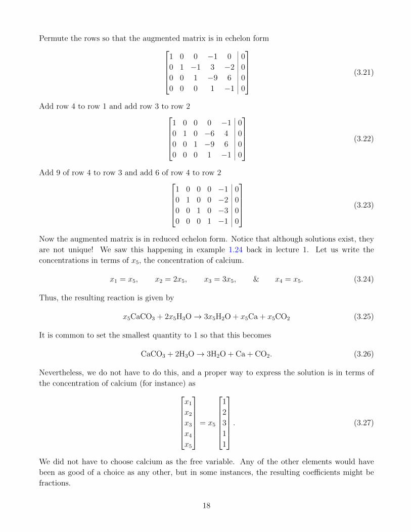
In the previous lecture, we saw how to think of matrices as linear transformations and vice

versa. If you think of a linear transformation as a process, you can perform processes in succession.

For example, imagine you had two linear transformations

Rm A Rnoooo (6.1)

and

Rl B Rmoooo . (6.2)

Here A is an m × n matrix and B is an l ×m matrix. Then it should be reasonable to perform

these operations in succession as

Rl B Rm A Rnoooooooo (6.3)

so that the result is some operation, denoted by BA, from Rn to Rl

Rl BA Rnoooo . (6.4)

In fact, we know we can do this because if ~x is a vector in Rn, we act on it with A to get a vector

A~x in Rm. Now that we have a vector in Rm we act on it with B to get a vector B(A~x) in Rl. This

operation of performing A first and then B is a linear transformation (exercise!) and therefore

must correspond to some unique matrix by Theorem 5.28. We call this matrix BA. In fact, we

can figure out a formula for its matrix components! Let’s try to do this. Let ~x be an arbitrary

vector in Rn. Then (3.2) gives

A~x =

a11 a12 · · · a1n

a21 a22 · · · a2n

......

...


x1

x2

...

xn

=


...

am1x1 + am2x2 + · · ·+ amnxn

(6.5)

where the vector on the right has m components. Now let’s act on this vector with B

B(A~x) =

b11 b12 · · · b1m

b21 b22 · · · b2m

......

...

bl1 bl2 · · · blm


...

am1x1 + am2x2 + · · ·+ amnxn

(6.6)

32

It looks complicated, but let us persevere and calculate this expression. To simplify things, let us

write the vector A~x using a shorthand notation as28a11x1 + a12x2 + · · ·+ a1nxna21x1 + a22x2 + · · ·+ a2nxn

...

am1x1 + am2x2 + · · ·+ amnxn

=

∑n

i=1 a1ixi∑ni=1 a2ixi

...∑ni=1 amixi

(6.7)

Using this notation, we can write

B(A~x) =

b11

∑ni=1 a1ixi + b12

∑ni=1 a2ixi + · · ·+ b1m

∑ni=1 amixi

b21

∑ni=1 a1ixi + b22

∑ni=1 a2ixi + · · ·+ b2m

∑ni=1 amixi

...

bl1∑n

i=1 a1ixi + bl2∑n

i=1 a2ixi + · · ·+ blm∑n

i=1 amixi

=

∑n

i=1 b11a1ixi +∑n

i=1 b12a2ixi + · · ·+∑n

i=1 b1mamixi∑ni=1 b21a1ixi +

∑ni=1 b22a2ixi + · · ·+

∑ni=1 b2mamixi

...∑ni=1 bl1a1ixi +

∑ni=1 bl2a2ixi + · · ·+

∑ni=1 blmamixi

=

∑ni=1

(b11a1i + b12a2i + · · ·+ b1mami

)xi∑n

i=1

(b21a1i + b22a2i + · · ·+ b2mami

)xi

...∑ni=1

(bl1a1i + bl2a2i + · · ·+ blmami

)xi

=

∑n

i=1 (∑m

k=1 b1kaki)xi∑ni=1 (

∑mk=1 b2kaki)xi

...∑ni=1 (

∑mk=1 blkaki)xi

,

(6.8)

which is now in the form needed to extract the matrix BA. By comparing this vector to the one

in (6.5), BA is the matrix

BA =

∑m

k=1 b1kak1

∑mk=1 b1kak2 · · ·

∑mk=1 bmkakn∑m

k=1 b2kak1

∑mk=1 b2kak2 · · ·

∑mk=1 b2kakn

......

...∑mk=1 blkak1

∑mk=1 blkak2 · · ·

∑mk=1 blkakn

(6.9)

From this calculation, we see that the (BA)ij component of the matrix BA is given by

(BA)ij :=m∑k=1

bikakj. (6.10)

28You should have seen this notation in calculus when learning about series.

33

The resulting formula seems overwhelming, but there is a convenient way to remember it instead

of this long derivation. The ij-th component of BA is given by multiplying the entries of the i-th

row of B with the entries of the j-th column of A and adding them all together: bi1 bi2 · · · · · · bim

a1j

a2j

...

amj

=

∑m

k=1 bikakj

(6.11)

This operation makes sense because the number of entries in a row of B is m while the number of

entries in a column of A is also m.

Example 6.12. Consider the following two linear transformations on R2 given by a shear S and

then a rotation R by angle θ (in the figures, k = 1 and θ = π2).

R2

[cos θ − sin θ

sin θ cos θ

]R2

[1 k

0 1

]R2oooooooo . (6.13)

R(S(~e1))R(S(~e2))

S(~e1)

S(~e2)

~e1

~e2

The resulting linear transformation is given by

R2

[cos θ k cos θ − sin θ

sin θ k sin θ − cos θ

]R2oooo , (6.14)

which with k = 1 and θ = π2

becomes

R2

[0 −1

1 1

]R2oooo (6.15)

If, however, we executed these operations in the opposite order

R2

[1 k

0 1

]R2

[cos θ − sin θ

sin θ cos θ

]R2oooooooo (6.16)

S(R(~e1))

S(R(~e2))

R(~e1)

R(~e2) ~e1

~e2

34

we would find the resulting linear transformation to be

R2

[k sin θ + cos θ k cos θ − sin θ

sin θ cos θ

]R2oooo , (6.17)

which with k = 1 and θ = π2

becomes

R2

[1 −1

1 0

]R2oooo (6.18)

Homework (Due: Tuesday September 20). Exercises 9, 10, 11, and 12 in Section 2.1 of [Lay].

Please show all your work, step by step! Do not use calculators or computer programs to solve

any problems! Notice how counterintuitive the results of these problems are. In addition to these

problems, mention how the results of problems 9, 10, 11, and 12 would change if the matrices were

1× 1 matrices instead.

35

7 September 20


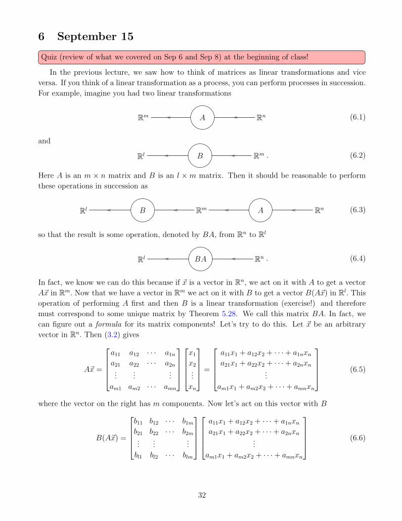
Given a linear transformation

Rm T Rnoooo (7.1)

taking vectors with n components in and providing vectors with m components out, you might want

to know if there is a way to go back to reverse the process. This would be a linear transformation

going in the opposite direction (I’ve drawn it going backwards to our usual convention)

Rm S Rn//// (7.2)

so that if we perform these two processes in succession, the result would be the transformation

that does nothing, i.e. the identity transformation. In other words, going along any closed loop in

the diagram

Rm

T

S

Rn

77''

ggww

(7.3)

is the identity. Expressed another way, this means that

ST Rn

nn

..

= 1n Rn

nn

..

(7.4)

and

TSRm

nn

..

= 1mRm

nn

..

(7.5)

Here 1m is the identity transformation on Rm and similarly 1n on Rn. Often, the inverse S of T

is written as T−1 and the inverse T of S is written as S−1. This is because inverses, if they exist,

are unique.

36

Definition 7.6. An m× n matrix A is invertible/nonsingular if there exists an n×m matrix B

such that

AB = 1n & BA = 1m. (7.7)

A matrix that is not invertible is called a noninvertible/singular matrix.

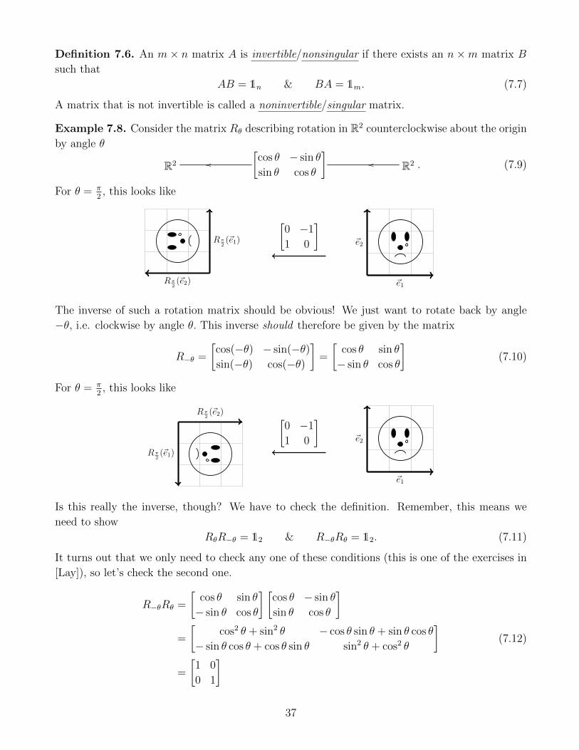
Example 7.8. Consider the matrix Rθ describing rotation in R2 counterclockwise about the origin

by angle θ

R2

[cos θ − sin θ

sin θ cos θ

]R2oooo . (7.9)


Rπ2(~e1)

Rπ2(~e2)

[0 −1

1 0

]

~e1

~e2

The inverse of such a rotation matrix should be obvious! We just want to rotate back by angle

−θ, i.e. clockwise by angle θ. This inverse should therefore be given by the matrix

R−θ =

[cos(−θ) − sin(−θ)sin(−θ) cos(−θ)

]=

[cos θ sin θ

− sin θ cos θ

](7.10)


Rπ2(~e1)

Rπ2(~e2) [

0 −1

1 0

]

~e1

~e2

Is this really the inverse, though? We have to check the definition. Remember, this means we

need to show

RθR−θ = 12 & R−θRθ = 12. (7.11)

It turns out that we only need to check any one of these conditions (this is one of the exercises in

[Lay]), so let’s check the second one.

R−θRθ =

[cos θ sin θ

− sin θ cos θ

] [cos θ − sin θ

sin θ cos θ

]=

[cos2 θ + sin2 θ − cos θ sin θ + sin θ cos θ

− sin θ cos θ + cos θ sin θ sin2 θ + cos2 θ

]=

[1 0

0 1

] (7.12)

37

Example 7.13. Consider the matrix S|k describing a vertical shear in R2 of length k

R2

[1 0

k 1

]R2oooo . (7.14)

When k = 1, this transformation is depicted by

S|1(~e1)

S|1(~e2)

[1 0

1 1

]

~e1

~e2

In this case as well, it seems intuitively clear that the inverse should be also vertical shear but

where the shift is in the opposite vertical direction, namely, k should be replaced with −k. Thus,

we propose that the inverse vertical shear, S|−k, is given by

S|−k =

[1 0

−k 1

]. (7.15)

When k = 1, this transformation is depicted by

S|1(~e1)

S|1(~e2)

[1 0

−1 1

]

~e1

~e2

We check that this works:

S|−kS

|k =

[1 0

−k 1

] [1 0

k 1

]=

[1 0

0 1

]. (7.16)

Theorem 7.17. A 2× 2 matrix

A :=

[a b

c d

](7.18)

is invertible if and only if ad− bc 6= 0. When this happens,

A−1 =1

ad− bc

[d −b−c a

]. (7.19)

38

The quantity ad − bc of a matrix as in this theorem is called the determinant of the matrix

A and is denoted by detA. In all of the examples, the matrices were square matrices, i.e. m × nmatrices where m = n. It turns out that an m × n matrix cannot be invertible if m 6= n. Our

examples from above are consistent with this theorem.

Example 7.20. In the 2 × 2 rotation matrix Rθ from our earlier examples, the determinant is

given by

detRθ = cos θ cos θ − sin θ(− sin θ) = cos2 θ + sin2 θ = 1. (7.21)

Example 7.22. In the 2× 2 vertical shear matrix S|k from our earlier examples, the determinant

is given by

detS|k = 1 · 1− 0 · k = 1. (7.23)

Invertible matrices are quite useful for the following reason.

Theorem 7.24. Let A be an invertible m×m matrix and let ~b be a vector in Rm. Then the linear

system

A~x = ~b (7.25)

has a unique solution. Furthermore, this solution is given by

~x = A−1~b. (7.26)

Exercise 7.27. Let

~b :=

[√3

1

](7.28)

and let Rπ/6 be the matrix that rotates by 30 (in the counterclockwise direction). Find the vector

~x whose image is ~b under this rotation.

Make the students answer this.

Steps:

(1) Write the matrix Rπ/6 explicitly.

(2) Draw the vector ~b.

(3) Guess a solution ~x by thinking about how Rπ/6 acts.

(4) Use the theorem to calculate ~x to test your guess.

(5) Compare your results and then make sure it works.

Theorem 7.29. If A is an invertible m×m matrix, then(A−1

)−1= A. (7.30)

If A and B are invertible m×m matrices, then AB is invertible and

(BA)−1 = A−1B−1. (7.31)

39

This theorem is completely intuitive! To reverse two processes, you do each one in reverse as

if you’re rewinding a movie! The inverse of an m × m matrix A can be computed, if it exists,

in the following way, reminiscent of how we solved linear systems. The idea is to row reduce the

augmented matrix [A 1m

](7.32)

to the form [1m B

](7.33)

where B is some new m×m matrix. If this can be done, B = A−1.

Example 7.34. The inverse of the matrix

A :=

1 −1 1

−1 1 0

1 0 1

(7.35)

can be calculated by some row reductions 1 −1 1 1 0 0

−1 1 0 0 1 0

1 0 1 0 0 1

7→1 −1 1 1 0 0

0 0 1 1 1 0

0 1 0 −1 0 1

7→1 0 1 0 0 1

0 0 1 1 1 0

0 1 0 −1 0 1

(7.36)

and then1 0 1 0 0 1

0 0 1 1 1 0

0 1 0 −1 0 1

7→1 0 0 −1 −1 1

0 0 1 1 1 0

0 1 0 −1 0 1

7→1 0 0 −1 −1 1

0 1 0 −1 0 1

0 0 1 1 1 0

(7.37)

So the supposed inverse is

A−1 =

−1 −1 1

−1 0 1

1 1 0

. (7.38)

To verify this, we should check that it works:−1 −1 1

−1 0 1

1 1 0

1 −1 1

−1 1 0

1 0 1

=

1 0 0

0 1 0

0 0 1

. (7.39)

Example 7.40. A rotation by angle θ (about the origin) in R3 in the plane spanned by ~e1 and ~e2

is given by the matrix cos θ − sin θ 0

sin θ cos θ 0

0 0 1

(7.41)

Theorem 7.42 (The Invertible Matrix Theorem). Please see [Lay] for this theorem. It provides

many characterizations for a matrix to be invertible.

40

Homework (Due: Tuesday September 27). Exercises 7, 21, 22, and 33 in Section 2.2 of [Lay],

Exercises 11 and 12 in Section 2.3 of [Lay], and Exercises 6 and 17 (ignore that it says to produce

an m×m matrix—please produce an (m−1)× (m−1) matrix that answers the questions—m = 3

for exercise 6 and m = 4 for exercise 17) in Section 2.7 of [Lay]. Warning: Please do not read

Section 2.7 in [Lay]. It may confuse you. Instead, refer to my notes. Please show all your work,

step by step! Do not use calculators or computer programs to solve any problems!

Recommended exercises include Exercises 9 (except part (e)), 13, 14, 23, 24, 25, 26, 34, 35 in

Section 2.2 of [Lay] and Exercises 13, 14, 21, 29, and 36 in Section 2.3 of [Lay].

41

8 September 22


Try to make the first half of this lecture a bit more interactive.

Definition 8.1. A subspace of Rn is a collection H of vectors in Rn satisfying the following

conditions.

(a) ~0 ∈ H.

(b) For every pair of vectors ~u and ~v in H, their sum ~u+ ~v is also in H.

(c) For every vector ~v and constant c, the scalar multiple c~v is in H.

Example 8.2. Rn itself is a subspace of Rn. Also, the set ~0 consisting of just the zero vector in

Rn is a subspace.

Are there other subspaces?

Exercise 8.3. Let H be the set of points in R3 described by the solution set of

3x− 2y + z = 0. (8.4)

See Figure 4. Is ~0 in H? Let

3x− 2y + z = 0

3x− 2y + z = 12

Figure 4: A plot of the planes described by 3x− 2y + z = 0 and 3x− 2y + z = 12.

~u =

u1

u2

u3

& ~v =

v1

v2

v3

(8.5)

be two vectors in H and let c be a real number. Is ~u+ ~v in H? Is c~v in H?

42

Exercise 8.6. Is the set of solutions to

3x− 2y + z = 12 (8.7)

a subspace of R3? See Figure 4. What goes wrong?

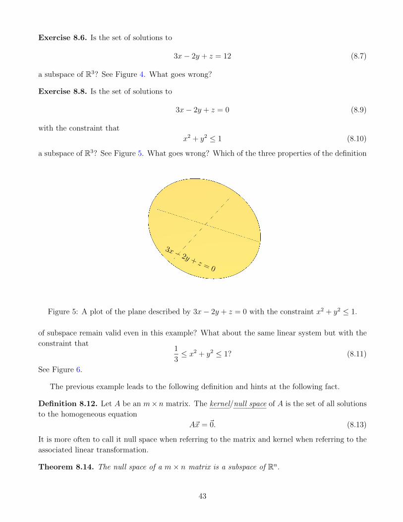
Exercise 8.8. Is the set of solutions to

3x− 2y + z = 0 (8.9)

with the constraint that

x2 + y2 ≤ 1 (8.10)

a subspace of R3? See Figure 5. What goes wrong? Which of the three properties of the definition

3x− 2y + z = 0

Figure 5: A plot of the plane described by 3x− 2y + z = 0 with the constraint x2 + y2 ≤ 1.

of subspace remain valid even in this example? What about the same linear system but with the

constraint that1

3≤ x2 + y2 ≤ 1? (8.11)

See Figure 6.

The previous example leads to the following definition and hints at the following fact.

Definition 8.12. Let A be an m×n matrix. The kernel/null space of A is the set of all solutions

to the homogeneous equation

A~x = ~0. (8.13)

It is more often to call it null space when referring to the matrix and kernel when referring to the

associated linear transformation.

Theorem 8.14. The null space of a m× n matrix is a subspace of Rn.

43

3x− 2y + z = 0

Figure 6: A plot of the plane described by 3x− 2y + z = 0 with the constraint 13≤ x2 + y2 ≤ 1.

Example 8.15. Consider the linear system

3x− 2y + z = 0 (8.16)

from the previous examples. The matrix corresponding to this linear system is just

A =[3 −2 1

], (8.17)

a 1 × 3 matrix. Hence, it describes a linear transformation from R3 to R1. The nullspace of A

exactly corresponds to the solutions of

[3 −2 1

] xyz

=[0]. (8.18)

Definition 8.19. Let A be an m×n matrix. The image/column space of A is the set of all vectors

in Rm of the form A~x with ~x in Rn. It is more often to call it column space when referring to the

matrix and image when referring to the associated linear transformation.

The reason the image of transformation Rm T←− Rn is called the column space is because the

image of T is spanned by the vectors in the columns of the associated matrixT (~e1) · · · T (~en)

(8.20)

In other words, ~b is in the image of A if and only if there exist coefficients x1, . . . , xn such that

~b = x1T (~e1) + · · ·+ xnT (~en). (8.21)

Theorem 8.22. The image of an m× n matrix is a subspace of Rm.

44

Example 8.23. Consider the linear transformation from R2 to R3 described by the matrix 1 0

0 1

−3 2

. (8.24)

The images of the vectors ~e1 and ~e2 get sent to the columns of the matrix. They span the plane

shown in Figure 7.

3x− 2y + z =0

Figure 7: A plot of the plane described by 3x− 2y + z = 0 along with two vectors spanning it.

Definition 8.25. A basis for a subspace H of Rn is a set of vectors that is both linearly independent

and spans H.

Exercise 8.26. Going back to our previous example of the plane in R3 specified by the linear

system

3x− 2y + z = 0, (8.27)

what is a basis for the vectors in this plane? Since the set of all vectorsxyz

(8.28)

satisfying this linear system define this plane, we just need to find a basis for these solutions. We

know that if we specify x and y as our free variables, then a general solution of this system is of

the form x

y

−3x+ 2y

(8.29)

45

with x and y free. How about testing the cases x = 1 with y = 0 and x = 0 with y = 1? This

gives 1

0

−3

&

0

1

2

(8.30)

respectively. Any other vector in the solution set is a linear combination of these two vectors.

Definition 8.31. The number of elements in a basis for a subspace H of Rn is the dimension of

H and is denoted by dimH.

Definition 8.32. Let A be an m× n matrix. The dimension of the image of A is also called the

rank of A and is denoted by rankA.

Theorem 8.33. Let A be an m× n matrix. Then

rankA+ dim kerA = n. (8.34)

Exercise 8.35. Check all of our examples to make sure you believe this.

Homework (Due: Tuesday September 27). Exercises 3, 4, and 16 in Section 2.8 of [Lay] and

Exercises 7 and 20 in Section 2.9 of [Lay]. Please show your work! Do not use calculators or

computer programs to solve any problems!

46

9 September 27


We’re going to do things a little differently from your book, so please pay close attention. Last

class, we defined the determinant of a 2× 2 matrix

A =

[a b

c d

](9.1)

to be

detA := ad− bc. (9.2)

We were partially motivated to give this quantity a special name because if detA 6= 0, then the

inverse of the matrix A is given by

A−1 =1

detA

[d −b−c a

]. (9.3)

There is another perspective to determinants that allows a simple generalization to higher dimen-

sions, i.e. for m×m matrices where m does not necessarily equal 2.

Example 9.4. Consider the following linear transformation.

A~e1

A~e2

A :=

[−2 2

1 0

]~e1

~e2

The square obtained from the vectors ~e1 and ~e2 gets transformed into a parallelogram obtained

from the vectors A~e1 and A~e2. The area (a.k.a. 2-dimensional volume) of the square is initially 1.

Under the transformation, the area becomes twice as big, so that gives a resulting area of 2. Also

notice that the orientation of the face gets flipped once (the tear is initially on the left side of the

face and after the transformation, it is on the right side). This is the same thing that happens to

you when you look in the mirror. It turns out that

detA = (sign of orientation)(volume of parallelogram) = (−1)(2) = −2, (9.5)

which we can check:

detA = (−2)(0)− (1)(2) = −2. (9.6)

Notice that if we swap the columns of A, then the transformation becomes

47

B~e1

B~e2B :=

[2 −2

0 1

]~e1

~e2

and the face is oriented the same way as in the original situation. The volume is scaled by 2 so we

expect the determinant to be 2, and it is:

detB = (2)(1)− (0)(−2) = 2. (9.7)

As another example, imagine writing the vector in the first column in the following way[2

0

]=

[2

1

]+

[0

−1

]. (9.8)

Then how is the determinant of B related to the determinants of the transformations

C~e1C~e2C :=

[2 −2

1 1

]~e1

~e2

and

D~e1

D~e2 D :=

[0 −2

−1 1

]~e1

~e2

48

A quick calculation shows that

detB = detC + detD

2 = 4− 2.(9.9)

The previous example illustrates many of the basic properties of the determinant function. For

a linear transformation Rm T←− Rm, the determinant of the resulting matrixT (~e1) · · · T (~em)

(9.10)

is the signed volume of the parallelepiped obtained from the column vectors in the above matrix.

The sign of the determinant is determined by the resulting orientation: +1 if the orientation

is right-handed and −1 if the orientation is left-handed. This definition has several important

properties, many of which have been illustrated in the previous example. The determinant for

m ×m matrices itself can be viewed as a function from m vectors in Rm to the real numbers R.These m vectors specify the parallelepiped in Rm and the function gives the signed volume of this

parallelepiped.

Definition 9.11. The determinant for m×m matrices is a function29

det :

m times︷︸︸︷Rm × · · ·Rm → R (9.12)

satisfying the following conditions.

(a) For every m-tuple of vectors (~v1, . . . , ~vm) in Rm,

det(~v1, . . . , ~vi, . . . , ~vj, . . . , ~vm

)

switch

= − det

(~v1, . . . , ~vj, . . . , ~vi, . . . , ~vm

). (9.13)

This is sometimes called the skew-symmetry of det .

(b) det is multilinear, i.e.

det(~v1, . . . , a~vi + b~ui, . . . , ~vm

)= a det

(~v1, . . . , ~vi, . . . , ~vm

)+ b det

(~v1, . . . , ~ui, . . . , ~vm

)(9.14)

for all i = 1, . . . ,m all scalars a, b and all vectors ~v1, . . . , ~vi−1, ~vi, ~ui, ~vi+1, . . . , ~vm.

(c) The determinant of the unit vectors, listed in order, is 1:

det(~e1, . . . , ~em

)= 1. (9.15)

For an m×m matrix A, the input for the determinant function consists of the columns of A

written in order:

detA := det(A~e1, · · · , A~em

). (9.16)

29I found this description of the determinant at http://math.stackexchange.com/questions/668/

whats-an-intuitive-way-to-think-about-the-determinant

49

http://math.stackexchange.com/questions/668/whats-an-intuitive-way-to-think-about-the-determinant

http://math.stackexchange.com/questions/668/whats-an-intuitive-way-to-think-about-the-determinant

Corollary 9.17. Let (~v1, . . . , ~vi, . . . , ~vj, . . . , ~vm) be a sequence of vectors in Rm where ~vi = ~vj (and

yet i 6= j). Then

det(~v1, . . . , ~vi, . . . , ~vi, . . . , ~vm

)= 0. (9.18)

Proof. By the skew-symmetry condition (a) in the definition of determinant,

det(~v1, . . . , ~vi, . . . , ~vj, . . . , ~vm

)

switch

= − det

(~v1, . . . , ~vj, . . . , ~vi, . . . , ~vm

)(9.19)

but since ~vi = ~vj

− det(~v1, . . . , ~vj, . . . , ~vi, . . . , ~vm

)= − det

(~v1, . . . , ~vi, . . . , ~vj, . . . , ~vm

). (9.20)

Putting these two equalities together gives

det(~v1, . . . , ~vi, . . . , ~vj, . . . , ~vm

)= − det

(~v1, . . . , ~vi, . . . , ~vj, . . . , ~vm

). (9.21)

A number can only equal the negative of itself if it is zero. Hence,

det(~v1, . . . , ~vi, . . . , ~vj, . . . , ~vm

)= 0 (9.22)

whenever ~vi = ~vj and i 6= j.

Corollary 9.23. Let (~v1, . . . , ~vi, . . . , ~vj, . . . , ~vm) be a list of m vectors in Rm. Then

det(~v1, . . . , ~vi, . . . , ~vj, . . . , ~vm

)= det

(~v1, . . . , ~vi + ~vj, . . . , ~vj, . . . , ~vm

)(9.24)

for any j between 1 and m.

Proof. This follows immediately from multilinearity and the previous Corollary

det(~v1, . . . , ~vi + ~vj, . . . , ~vj, . . . , ~vm

)= det

(~v1, . . . , ~vi, . . . , ~vj, . . . , ~vm

)+ det

(~v1, . . . , ~vj, . . . , ~vj, . . . , ~vm

)︸︷︷︸

0

(9.25)

because ~vj repeats itself in the argument of det .

Let’s check to make sure this definition reduces to the determinant of a 2× 2 matrix. Let

A :=

[a b

c d

]. (9.26)

Then the columns of A are ([a

c

],

[b

d

])= (a~e1 + c~e2, b~e1 + d~e2) . (9.27)

50

Therefore,

detA = det (a~e1 + c~e2, b~e1 + d~e2)

= a det (~e1, b~e1 + d~e2) + c det (~e2, b~e1 + d~e2)

= ab det (~e1, ~e1)︸︷︷︸0

+ad det (~e1, ~e2)︸︷︷︸1

+cb det (~e2, ~e1)︸︷︷︸−1

+cd det (~e2, ~e2)︸︷︷︸0

= ad− bc.

(9.28)

Wow! This abstract technique actually worked! And we didn’t have to memorize all the formulas

in your textbook. All we have to remember are the three conditions in Definition 9.11.

Example 9.29. Let’s try an example in R3 this time before figuring out the general formula. Let

A :=

1 1 0

2 0 1

0 −1 1

. (9.30)

Then

detA = det (A~e1, A~e2, A~e3)

= det (~e1 + 2~e2, ~e1 − ~e3, ~e2 + ~e3)

= det (~e1, ~e1 − ~e3, ~e2 + ~e3) + 2 det (~e2, ~e1 − ~e3, ~e2 + ~e3)

= det (~e1, ~e1, ~e2 + ~e3)︸︷︷︸0

− det (~e1, ~e3, ~e2 + ~e3)

+ 2 det (~e2, ~e1, ~e2 + ~e3)− 2 det (~e2, ~e3, ~e2 + ~e3)

= − det (~e1, ~e3, ~e2)︸︷︷︸−1

− det (~e1, ~e3, ~e3)︸︷︷︸0

+2 det (~e2, ~e1, ~e2)︸︷︷︸0

+ 2 det (~e2, ~e1, ~e3)︸︷︷︸−1

−2 det (~e2, ~e3, ~e2)︸︷︷︸0

−2 det (~e2, ~e3, ~e3)︸︷︷︸0

= −1.

(9.31)

With this general idea, you can calculate determinants of very large matrices as well, though

perhaps it may take a lot of time.

Homework (Due: Tuesday October 4). Please check HuskyCT for the homework. Please show

your work! Do not use calculators or computer programs to solve any problems!

51

10 September 29


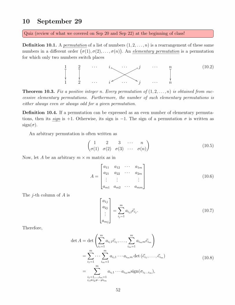
Definition 10.1. A permutation of a list of numbers (1, 2, . . . , n) is a rearrangement of these same

numbers in a different order(σ(1), σ(2), . . . , σ(n)

). An elementary permutation is a permutation

for which only two numbers switch places

1_

2_

· · · i

''

· · · j/

ww

· · · n_

1 2 · · · i · · · j · · · n

(10.2)

Theorem 10.3. Fix a positive integer n. Every permutation of (1, 2, . . . , n) is obtained from suc-

cessive elementary permutations. Furthermore, the number of such elementary permutations is

either always even or always odd for a given permutation.

Definition 10.4. If a permutation can be expressed as an even number of elementary permuta-

tions, then its sign is +1. Otherwise, its sign is −1. The sign of a permutation σ is written as

sign(σ).

An arbitrary permutation is often written as(1 2 3 · · · n

σ(1) σ(2) σ(3) · · · σ(n)

)(10.5)

Now, let A be an arbitrary m×m matrix as in

A =

a11 a12 · · · a1m

a21 a22 · · · a2m

......

...

am1 am2 · · · amm

(10.6)

The j-th column of A is a1j

a2j

...

amj

=m∑ij=1

aijj~eij . (10.7)

Therefore,

detA = det

(m∑i1=1

ai11~ei1 , . . . ,m∑

im=1

aimm~eim

)

=m∑i1=1

· · ·m∑

im=1

ai11 · · · aimm det (~ei1 , . . . , ~eim)

=m∑

i1=1,...,im=1i1 6=i2 6=···6=im

ai11 · · · aimmsign(σi1...im),

(10.8)

52

where σi1...im is the permutation defined by(1 2 · · · m

i1 i2 · · · im

). (10.9)

In the second equality in (10.8), the multi-linearity of det was used. In the third equality, the

skew-symmetry of det was used together with the fact that the determinant of the identity matrix

is 1.

Example 10.10. Let’s use this formula to find a more memorable formula for the determinant of

a 3× 3 matrix. Let the 3× 3 matrix be of the form

A :=

a11 a12 a13

a21 a22 a23

a31 a32 a33

(10.11)

Then,

detA =3∑

i1=1,i2=1,i3=1i1 6=i2 6=i3

ai11ai22ai33sign(σi1i2i3)

= a11

3∑i2=2,i3=2i2 6=i3

ai22ai33sign(σ1i2i3) + a12

3∑i1=2,i3=2i1 6=i3

ai11ai33sign(σi11i3) + a13

3∑i1=2,i2=2i1 6=i2

ai11ai22sign(σi1i21)

= a11

3∑i2=2,i3=2i2 6=i3

ai22ai33sign(σi2i3)− a12

3∑i1=2,i3=2i1 6=i3


3∑i1=2,i2=2i1 6=i2


= a11(a22a33 − a32a23)− a12(a21a33 − a31a23) + a13(a21a32 − a31a22)

= a11 det

[a22 a23

a32 a33

]− a12 det

[a21 a23

a31 a33

]+ a13 det

[a21 a22

a31 a32

]≡ a11 detA11 − a12 detA12 + a13 detA13

(10.12)

by some rearrangements of the terms. In the last equality, we have introduced the notation A1j.

This is the resulting matrix obtained from A by deleting the 1-st row and j-th column

A11 :=

a11 a12 a13

a21 a22 a23

a31 a32 a33

, A12 :=

a11 a12 a13

a21 a22 a23

a31 a32 a33

, & A13 :=

a11 a12 a13

a21 a22 a23

a31 a32 a33

. (10.13)

Note that we could have chosen to do this rearrangement by separating out the second or third

row instead of the first. Just to illustrate the slight difference, let’s separate out the second row

53

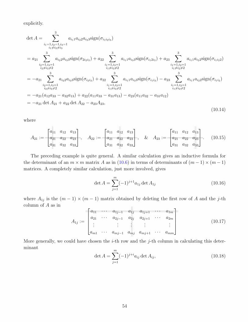
explicitly.

detA =3∑

i1=1,i2=1,i3=1i1 6=i2 6=i3

ai11ai22ai33sign(σi1i2i3)

= a21

3∑i2=1,i3=1i2 6=i3 6=2

ai22ai33sign(σ2i2i3) + a22

3∑i1=1,i3=1i1 6=i3 6=2


3∑i1=1,i2=1i1 6=i2 6=2


= −a21

3∑i2=1,i3=1i2 6=i3 6=2


3∑i1=1,i3=1i1 6=i3 6=2

ai11ai33sign(σi1i3)− a23

3∑i1=1,i2=1i1 6=i2 6=2


= −a21(a12a33 − a32a13) + a22(a11a33 − a31a13)− a23(a11a32 − a31a12)

= −a21 detA21 + a22 detA22 − a23A23,

(10.14)

where

A21 :=

a11 a12 a13

a21 a22 a23

a31 a32 a33

, A22 :=

a11 a12 a13

a21 a22 a23

a31 a32 a33

, & A23 :=

a11 a12 a13

a21 a22 a23

a31 a32 a33

. (10.15)

The preceding example is quite general. A similar calculation gives an inductive formula for

the determinant of an m×m matrix A as in (10.6) in terms of determinants of (m− 1)× (m− 1)

matrices. A completely similar calculation, just more involved, gives

detA =m∑j=1

(−1)j+1a1j detA1j (10.16)

where A1j is the (m − 1) × (m − 1) matrix obtained by deleting the first row of A and the j-th

column of A as in

A1j :=

a11 · · · a1j−1 a1j a1j+1 · · · a1m

a21 · · · a2j−1 a2j a2j+1 · · · a2m

......

......

...

am1 · · · amj−1 amj amj+1 · · · amm

(10.17)

More generally, we could have chosen the i-th row and the j-th column in calculating this deter-

minant

detA =m∑j=1

(−1)j+iaij detAij, (10.18)

54

where

Aij :=

a11 · · · a1j−1 a1j a1j+1 · · · a1m

......

......

...

ai−11 · · · ai−1j−1 ai−1j ai−1j+1 · · · ai−1m

ai1 · · · aij−1 aij aij+1 · · · aimai+11 · · · ai+1j−1 ai+1j ai+1j+1 · · · ai+1m

......

......

...

am1 · · · amj−1 amj amj+1 · · · amm

(10.19)

Definition 10.20. Let A be an m×m matrix as above. In the previous formula for the determi-

nant,

Cij := (−1)i+j detAij (10.21)

is called the (i, j)-cofactor of A.

Theorem 10.22. Let A be an m×m matrix. A is invertible if and only if detA 6= 0. Furthermore,

when this happens,

A−1 =1

detA

C11 C21 · · · Cm1

C12 C22 · · · Cm2

......

...

C1m C2m · · · Cmm

, (10.23)

where Cij is the (i, j)-cofactor of A.

Definition 10.24. The transpose of an m× n matrix A

A =

a11 a12 · · · a1n

a21 a22 · · · a2n

......

...


(10.25)

is the n×m matrix

AT :=

a11 a21 · · · an1

a12 a22 · · · an2

......

...

a1m a2m · · · anm

. (10.26)

Theorem 10.27. Let A be an m×m matrix. Then

detAT = detA. (10.28)

Definition 10.29. The matrixC11 C21 · · · Cm1

C12 C22 · · · Cm2

......

...

C1m C2m · · · Cmm

≡C11 C12 · · · C1m

C21 C22 · · · C2m

......

...

Cm1 Cm2 · · · Cmm

T

(10.30)

in Theorem 10.22 is called the adjugate of A. It is often written as adjA.

55

The following facts follow from everything we have done so far.

Theorem 10.31. An m×m matrix A is invertible if and only if its columns form a basis of Rm.

From the definition of the transpose of a matrix, the definition of the determinant, and Corollary

9.23, one can calculate the determinant using row operations. Swapping rows introduces a minus

sign from the definition of det . Adding rows does not change anything by this theorem and

Corollary 9.23. And in your homework, you are asked to find a formula for the determinant of an

upper-triangular matrix. In other words, if a matrix A is row reduced to a matrix A′ without any

scaling of rows, then

detA = (−1)number of row swaps detA′. (10.32)

This is a faster method for computing the determinant.



56

11 October 4

Today is a review session. A practice exam has been uploaded to HuskyCT.

57

12 October 6

Today is the first midterm.

58

13 October 11


We didn’t finish a lot of material from the sections on determinants since we ended while still

working through example 10.10. So look back to that example now since I think most of today

will be on that.

Example 13.1. Let’s find the inverse of the matrix

A :=

1 1 3

2 −2 1

0 1 0

. (13.2)

The determinant of A is

detA = 1 · det

[1 3

2 1

]= 1− 6 = −5. (13.3)

The adjugate matrix of A is given by

adjA :=

det

[−2 1

1 0

]− det

[2 1

0 0

]det

[2 −2

0 1

]− det

[1 3

1 0

]det

[1 3

0 0

]− det

[1 1

0 1

]det

[1 3

−2 1

]− det

[1 3

2 1

]det

[1 1

2 −2

]

T

=

−1 0 2

3 0 −1

7 5 −4

T

=

−1 3 7

0 0 5

2 −1 −4

. (13.4)

Therefore,

A−1 =1

detAadjA =

1

5

−1 3 7

0 0 5

2 −1 −4

. (13.5)

Let’s just make sure this works:

A−1A =1

5

−1 3 7

0 0 5

2 −1 −4

1 1 3

2 −2 1

0 1 0

=

1

5

−1 + 6 + 0 −1− 6 + 7 −3 + 3 + 0

0 + 0 + 0 0 + 0 + 5 0 + 0 + 0

2− 2 + 0 2 + 2− 4 6− 1 + 0

=

1 0 0

0 1 0

0 0 1

.(13.6)

59

Definition 13.7. A real vector space consists of a set V, the elements of which are called vectors,

together with

i) a binary operation + : V × V → V, called addition and written as ~u+ ~v

ii) a vector ~0 in V, called the zero vector

iii) a function R× V → V, called scalar multiplication and written as c~u

satisfying

(a) addition is commutative: ~u+ ~v = ~v + ~u

(b) addition is associative: ~u+ (~v + ~w) = (~u+ ~v) + ~w

(c) the zero vector is an identity for addition: ~u+~0 = ~u

(d) addition is invertible: for each vector ~u, there is a vector ~v such that ~u+ ~v = ~0

(e) scalar multiplication is distributive over vector addition: c(~u+ ~v) = c~u+ c~v

(f) scalar multiplication is distributive over scalar addition: (c+ d)~u = c~u+ d~u

(g) scalar multiplication is distributive over itself: c(d~u) = (cd)~u

(h) the scalar unit axiom: 1~u = ~u

As you can see, the definition of a vector space is very complicated! There are so many things

to check (compare this to when we were checking whether something was a subspace)! On the

one hand, they are complicated in the sense that there are many data and several restrictions.

On the other hand, all these restrictions make them more manageable and therefore easier to

understand. In particular, vector spaces are completely characterized by their dimension (we will

later define dimension, but you probably already have a rough idea): if two vector spaces have the

same dimension, then they are isomorphic, which means that the only difference between them

is in the description, but there is no difference between them with respect to their vector space

structures. If you take a course in abstract algebra, you’ll learn what a group is. An abelian group

consists of a set with structure (i) and (ii) from above and satisfying (a), (b), (c), and (d). Abelian

groups therefore have less structure, but also fewer restrictions.

You might also ask: why do we need such an abstract definition? What do we gain? The

pay-off is actually phenomenal. As we will see shortly, there are many examples of vector spaces.

Rather than proving something about each and every one of these examples, if we can prove or

discover something for general vector spaces, then all of these results will hold for every single

example.

Example 13.8. Rn whose elements are viewed as n-component column vectors, together with

component-wise addition, the vector whose entries are all 0 as the zero vector, and scalar multi-

plication defined component-wise (as in the first few lectures), is a vector space.

60

Example 13.9. Any subspace of Rn is a vector space with the induced addition, zero vector, and

scalar multiplication.

Example 13.10. The set ofm×nmatrices is a vector space with addition given by component-wise

addition, the zero vector is the zero matrix, and the scalar multiplication is given by distributing

the scalar to each component. This vector space is denoted by mMn.

With the last example, how can we visualize the sum of matrices? We know how to visualize

the sum of n-component vectors (at least when n ≤ 3) as appending the tail of one vector at the

head of the other. This idea won’t work for m × n matrices when m,n ≥ 2 because there are at

least 4 entries and we can’t visualize more than 3 dimensions. However, we can think of addition

in the following way. Let

A :=

[0 −1

1 0

]and B :=

[1 1

0 1

](13.11)

be rotation by 90 and a horizontal shear, respectively. Let t be a variable between 0 and 1. Then

we can look at

tA+B =

[1 1− tt 1

]and A+ tB =

[t t− 1

1 t

]. (13.12)

When t = 1, both of these give A+B, which is

A+B =

[1 0

1 1

], (13.13)

but as t varies and is initially small, we either have B or A for small values of t and then as t

increases we see the additional contribution from the other matrix.Draw this.

Example 13.14. A degree n polynomial is a function p of the form

p(x) = a0 + a1x+ a2x2 + · · ·+ anx

n, (13.15)

where a0, a1, a2, . . . , an are real numbers. A degree zero polynomial is a constant, a degree one

polynomial is a linear function, and a degree two polynomial is a quadratic function. The sum of

two degree n polynomials p as above and q given by

q(x) = b0 + b1x+ b2x2 + · · ·+ bnx

n (13.16)

is the degree n polynomial p+ q, which is given by

(p+ q)(x) := p(x) + q(x) ≡ (a0 + b0) + (a1 + b1)x+ (a2 + b2)x2 + · · ·+ (an + bn)xn. (13.17)

If c is a real number, then cp is the degree n polynomial given by

(cp)(x) := cp(x) ≡ ca0 + ca1x+ ca2x2 + · · ·+ canx

n. (13.18)

The zero polynomial is just the polynomial whose coefficients are all zero, i.e. it’s the constant

function whose value is always zero. Then this gives the set of degree n polynomials the structure

of a vector space. We denote this vector space by Pn.

61

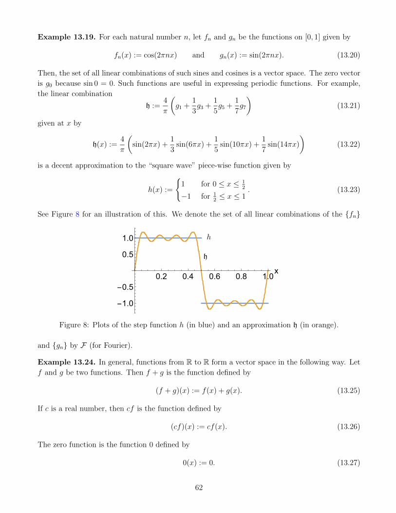
Example 13.19. For each natural number n, let fn and gn be the functions on [0, 1] given by

fn(x) := cos(2πnx) and gn(x) := sin(2πnx). (13.20)

Then, the set of all linear combinations of such sines and cosines is a vector space. The zero vector

is g0 because sin 0 = 0. Such functions are useful in expressing periodic functions. For example,

the linear combination

h :=4

π

(g1 +

1

3g3 +

1

5g5 +

1

7g7

)(13.21)

given at x by

h(x) :=4

π

(sin(2πx) +

1

3sin(6πx) +

1

5sin(10πx) +

1

7sin(14πx)

)(13.22)

is a decent approximation to the “square wave” piece-wise function given by

h(x) :=

1 for 0 ≤ x ≤ 1

2

−1 for 12≤ x ≤ 1

. (13.23)

See Figure 8 for an illustration of this. We denote the set of all linear combinations of the fn

0.2 0.4 0.6 0.8 1.0x

-1.0

-0.5

0.5

1.0 h

h

Figure 8: Plots of the step function h (in blue) and an approximation h (in orange).

and gn by F (for Fourier).

Example 13.24. In general, functions from R to R form a vector space in the following way. Let

f and g be two functions. Then f + g is the function defined by

(f + g)(x) := f(x) + g(x). (13.25)

If c is a real number, then cf is the function defined by

(cf)(x) := cf(x). (13.26)

The zero function is the function 0 defined by

0(x) := 0. (13.27)

62

Example 13.28. Let (a1, a2, a3, . . . ) be a sequence of real numbers satisfying

∞∑n=1

|an| <∞, (13.29)

(recall, this means∑∞

n=1 an is an absolutely convergent series). Given another sequence of real

numbers (b1, b2, b3, . . . ) satisfying∞∑n=1

|bn| <∞, (13.30)

we define the sum of the two to be given by

(a1, a2, a3, . . . ) + (b1, b2, b3, . . . ) := (a1 + b1, a2 + b2, a3 + b3, . . . ). (13.31)

The zero vector is the sequence (0, 0, 0, . . . ). If c is a real number, then the scalar multiplication is

defined to be

c(a1, a2, a3, . . . ) := (ca1, ca2, ca3, . . . ). (13.32)

The sum of two sequences still satisfies the absolutely convergent condition because

∞∑n=1

|an + bn| ≤∞∑n=1

(|an|+ |bn|

)=∞∑n=1

|an|+∞∑n=1

|bn| <∞ (13.33)

by the triangle inequality. Furthermore, the scalar multiplication of an absolutely convergent series

is still absolutely convergent

∞∑n=1

|can| =∞∑n=1

|c||an| = |c|∞∑n=1

|an| <∞. (13.34)

The set of such sequences whose associated series are absolutely convergent is denoted by `1.

Exercise 13.35. A closely related example of a vector space that shows up in quantum mechanics

is the set of sequence of complex numbers (a1, a2, a3, . . . ) such that

∞∑n=1

|an|2 <∞. (13.36)

The zero vector, sum, and scalar multiplication are defined just as in Example 13.28. Check that

this is a vector space (this vector space is denoted by `2).

Exercise 13.37. A generalization of the vector spaces `1 and `2 is the following. Let p ≥ 1. The

set of sequences (a1, a2, a3, . . . ) satisfying

∞∑n=1

|an|p <∞, (13.38)

with similar structure as in the previous examples, is a vector space. This space is denoted by `p.



63

14 October 13

Today, we will define subspaces, linear transformations, the kernel (a.k.a. nullspace), and the

image (a.k.a. column space) of a linear transformation. We briefly discussed this for matrices

before, but will repeat it from this more general perspective.

Definition 14.1. If V is a vector space, a subspace of V is a subset H of V satisfying the axioms

in Definition 8.1.

Theorem 14.2. If V is a vector space and W is a subspace of V, then W is a vector space.

Exercise 14.3. Show that `1 is a subspace of `2. Note that `1 was defined in Example 13.28 and

`2 was defined in Example 13.35 (let both of the sequences be either real or complex). [Warning:

this exercise is not trivial.]

Exercise 14.4. Show that `2 is not a subspace of `1. [Hint: give an example of a sequence

(a1, a2, a3, . . . ) such that∑∞

n=1 |an|2 <∞ but∑∞

n=1 |an| does not converge.]

Definition 14.5. Let V and W be two vector spaces. A linear transformation WT←− V from V

to W is a function from V to W satisfying

T (c~v) = cT (~v) and T (~v1 + ~v2) = T (~v1) + T (~v2). (14.6)

Example 14.7. In the above definition, if V = Rn and W = Rm, then a linear transformation T

uniquely corresponds to an m× n matrix.

Example 14.8. Let Pn be the vector space of degree n polynomials (in the variable x). The

function Pn+1T←− Pn, given by (

T (p))(x) := xp(x) (14.9)

for any degreen n polynomial p, is a linear transformation. Here p is a degree n polynomial and

T (p) is a degree n+ 1 polynomial. For example, if n = 1 and p is of the form p(x) = mx+ b with

m and b real numbers, then T (p) is the quadratic polynomial given by mx2 + bx.

Definition 14.10. Let V and W be two vector spaces and let WT←− V be a linear transformation

from V to W. The kernel of T, written as kerT, is the set of vectors ~v in V satisfying T (~v) = ~0.

The image of T is the set of vectors of the form T (~v) in W with ~v in V.

Example 14.11. In the case that V = Rn and W = Rm, a linear transformation T uniquely

corresponds to an m×n matrix A. In this case, the kernel/null space of T is the set of all solutions

~x to the homogeneous equation

A~x = ~0. (14.12)

The image/column space of T is the set of all vectors in Rm of the form A~x with ~x in Rn. It is

more often to call it column space when referring to the matrix and image when referring to the

associated linear transformation.

Theorem 14.13. The kernel of a linear transformation WT←− V is a subspace of V.

64

Theorem 14.14. The image of a linear transformation WT←− V is a subspace of W.

Example 14.15. Let Pn+1T←− Pn be the linear transformation from Example 14.8. The image

(column space) of this linear transformation is the set of degree n+ 1 polynomials of the form

a1x+ a2x2 + · · ·+ anx

n + an+1xn+1. (14.16)

In other words, it is the set of all polynomials with no constant term.

Problem 14.17. Let30

A :=

[1 2 4 0

0 1 3 −2

]. (14.18)

Describe the kernel/null space of A. Give an example of a basis for the kerA.

Answer. The kernel of A consists of vectors ~x in R4 satisfying A~x = ~0. Solving this linear system

gives x1

x2

x3

x4

=

2x3 − 4x4

−3x3 + 2x4

x3

x4

= x3

2

−3

1

0

+ x4

−4

2

0

1

, (14.19)

where x3 and x4 are free variables. One basis for this kernel is therefore given by

2

−3

1

0

,−4

2

0

1

. (14.20)


your work! Do not use calculators or computer programs to solve any problems! Today, we finished

Sections 4.1 and 4.2 of [Lay].

30This is Exercise 4.2.3 in [Lay].

65

15 October 18

HW #06 is due at the beginning of class! Give time for questions.

I think we went through a few too many concepts from last class. In particular, I mentioned

basis and dimension, but I didn’t exactly say what it means for a set of vectors in an arbitrary

vector space to span the space or when they are linearly independent. The definition is almost the

same as it was before, but it’s good to review it anyway.

Definition 15.1. Let V be a vector space. A set of vectors S := ~v1, . . . , ~vk in V is linearly

independent if the only values of x1, . . . , xk that satisfy the equation

k∑i=1

xi~vi ≡ x1~v1 + · · ·+ xk~vk = ~0 (15.2)

are

x1 = 0, x2 = 0, . . . , xk = 0. (15.3)

A set S of vectors as above is linearly dependent if there exists a solution to the above equation

for which not all of the xi’s are zero. If S is an infinite set of vectors in V, indexed, say, by some

set Λ so that S = ~vαα∈Λ, then S is linearly independent if for every finite subset Ω of Λ, the

only solution to31 ∑α∈Ω

xα~vα = ~0 (15.4)

is

xα = 0 for all α ∈ Ω. (15.5)

S is linearly dependent if it is not linearly independent, i.e. if there exists a finite subset Ω of Λ

with a solution to∑

α∈Ω xα~vα = ~0 in which not all of the xα’s is 0.

Example 15.6. Let S be the set of degree 7 polynomials of the form S := p1, p3, p7. Here pk is

the k-th degree monomial

pk(x) = xk. (15.7)

The set S is linearly independent. This is because the only solution to

a1x+ a3x3 + a7x

7 = 0 (15.8)

that holds for all x is

a1 = a3 = a7 = 0. (15.9)

However, the set p1, p3, 3p3−7p7, p7 is linearly dependent because the third entry can be written

as a linear combination of the other entries. The set p1 + 2p3, p4 − p5, 3p6 + 5p0 − p1 is linearly

independent. This is because the only solution to

a(x+ 2x3) + b(x4 − x5) + c(3x6 + 5− x) = 0 (15.10)

31Here, the notation α ∈ Ω means that α is an element of Ω.

66

is a = b = c = 0. To see this, rewrite the left-hand-side as

a(x+ 2x3) + b(x4 − x5) + c(3x6 + 5− x) = c5 + (a− c)x+ a2x3 + bx4 − bx5 + c3x6. (15.11)

The only way the right-hand-side vanishes for all values of x is when c = 0 which then forces a = 0

and b = 0 as well.

Example 15.12. The set of 2× 2 matrices

A :=

[1 2

0 −1

], B :=

[−3 1

0 2

], and C :=

[−1 5

0 0

](15.13)

are linearly dependent because

2A+B = C. (15.14)

Theorem 15.15. Let V be a vector space and let S be a set of vectors in V. The set S is linearly

dependent if and only if at least one of the vectors in S can be written as a linear combination of

the other vectors in S.

Definition 15.16. Let V be a vector space and let S := ~v1, . . . , ~vk be a set of k vectors in V.

The span of S is the set of vectors in V of the form

k∑i=1

xi~vi ≡ x1~v1 + · · ·xk~vk, (15.17)

with x1, . . . , xk arbitrary real numbers. The span of S is often denoted by span(S). If S is an

infinite set of vectors, say indexed by some set Λ, in which case S is written as S := ~vαα∈Λ, then

the span of S is the set of vectors in V of the form32∑α∈Ω⊆Λ

Ω is finite

xα~vα. (15.18)

Remark 15.19. The sum in the definition of span must be finite (even if S itself is infinite).

At this point, it does not make sense to take an infinite sum of vectors (to make sense of this,

we would have to talk about convergence and would have to define a notion of distance between

different vectors, which we have not (yet) done.

Proposition 15.20. Let V be a vector space and S a set of vectors in V. Then the span of S is a

subspace of V.

Example 15.21. Consider the vector space F of Example 13.19. Recall, this is the vector space

of linear combinations of the functions fn(x) := cos(2πnx) and gm(x) := sin(2πmx) for arbitrary

natural numbers n and m. Let S := f0, f1, g1, f2, g2, f3, g3, . . . . Then the function

x 7→ sin(

2πx− π

4

)(15.22)

32Here, the notation Ω ⊆ Λ means that Ω is a subset of Λ and α ∈ Ω means that α is an element of Ω.

67

is in the span of S. Notice that this function is not in the set S. The fact that this function is in

the span follows from the sum angle formula for sine:

sin(θ + φ) = sin(θ) cos(φ) + cos(θ) sin(φ), (15.23)

which gives

sin(

2πx− π

4

)= sin(2πx) cos

(−π

4

)+ cos(2πx) sin

(−π

4

)=

√2

2sin(2πx)−

√2

2cos(2πx)

=

√2

2g1(x) +

(−√

2

2

)f1(x).

(15.24)

As another example, the function

x 7→ cos2(2πx) (15.25)

is also in the span of S. For this, recall the other angle sum formula

cos(θ + φ) = cos(θ) cos(φ)− sin(θ) sin(φ) (15.26)

and of course the identity

cos2(θ) + sin2(θ) = 1, (15.27)

which can be used to rewrite

cos(2θ) = cos2(θ)− sin2(θ) = cos2(θ)−(

1− cos2(θ))

= 2 cos2(θ)− 1. (15.28)

Using this last identity, we can write

cos2(2πx) =1

2+

1

2cos(4πx) =

1

2f0(x) +

1

2f2(x). (15.29)

Definition 15.30. Let V be a vector space. A basis of V is a set B of vectors in V that is linearly

independent and spans V.

Theorem 15.31. Let V be a vector space with a basis B consisting of n elements (here n is a

natural number). If S is another basis of V, then S consists of n elements as well.

Definition 15.32. The number of elements in a basis for a vector space V is the dimension of V

and is denoted by dimV. A vector space V with dimV < ∞ is said to be finite-dimensional. A

vector space V with dimV =∞ is said to be infinite-dimensional.

Example 15.33. A basis of Pn is given by the monomials (p0, p1, p2, . . . , pn), where

pk(x) := xk. (15.34)

Therefore, dimPn = n+ 1.

68

Example 15.35. A basis for m× n matrices is given by matrices of the form

Eij :=

0 · · · 0 0 0 · · · 0...

......

......

0 · · · 0 0 0 · · · 0

0 · · · 0 1 0 · · · 0

0 · · · 0 0 0 · · · 0...

......

......

0 · · · 0 0 0 · · · 0

(15.36)

where the only non-zero entry is in the i-th row and j-th column, where its value is 1. In other

words, Eij is an m × n matrix with a 1 in the i-th row and j-th column and is zero everywhere

else. Therefore, dimmMn := mn.

Example 15.37. Let F be the vector space from Example 13.19. A basis for F is given by

f0, f1, g1, f2, g2, . . . . Then dimF =∞.

Theorem 15.38. Let V be a vector space and let S be a set of vectors in V. Let H := span(S).

(a) Let ~v be a vector in S. If ~v is in the span of S \ ~v, i.e. the set S with ~v removed, then

span(S \ ~v) = H.

(b) If H is not the zero subspace, then there exists a subset B of S such that B is a basis of H.

Problem 15.39. Consider the following four vectors in R3

~v1 :=

1

2

3

, ~v2 :=

1

−1

−2

, ~v3 :=

0

0

0

, and ~v4 :=

5

4

5

, (15.40)

Is S := ~v1, ~v2, ~v3, ~v4 a basis for span(S)? If not, find a subset B of S that is a basis for span(S).

Find the dimension of span(S).

Answer. No, the set S is not a basis because the set is not linearly independent. One can

remove ~v3 and ~v4 from S and still have a linearly independent set. ~v4 can be removed because

~v4 = 3~v1 + 2~v2. Therefore, we can take B to be B := ~v1, ~v2. This is a basis for span(S) because

it is linearly independent and spans this space. The dimension is therefore 2.


your work! Do not use calculators or computer programs to solve any problems! In this lecture,

we covered Section 4.3 and parts of Section 4.5.

69

16 October 20

Quiz (review of what we covered on Sep 29, Oct 11, and Oct 13) at the beginning of class!

The following theorems help one understand the concept of a basis more.

Theorem 16.1. Let V be a vector space and let H be a subspace of V. Then dim(H) ≤ dim(V ).

Theorem 16.2. Let V be a vector space and let B be a basis for V. Then every vector ~v in V can

be written uniquely as a linear combination of elements of B (except for possibly zero weights).

Note that this theorem is false if the word “basis” is replaced with a set that merely spans V.

Also, the theorem is true even in infinite-dimensional vector spaces.

Proof. To cover the case of infinite dimensions as well, let B = ~vαα∈Λ and suppose that the

vector ~u can be expressed as a linear combination of the vectors in S in two ways as

~u =∑

α∈Ω⊆ΛΩ finite

xα~vα and ~u =∑

β∈Θ⊆ΛΩ finite

yβ~vβ (16.3)

Then the difference of these two equals the zero vector and is given by the sum∑α∈Ω but α/∈Θ

xα~vα +∑

α∈Ω and α∈Θ

(xα − yα)~vα +∑

α/∈Ω but α∈Θ

yα~vα = ~0. (16.4)

Here the notation α /∈ Ω means that α is not an element of Ω. Because the vectors ~vα are all

linearly independent, this is only possible if all of the coefficients are zero.

In the case that the vector space was infinite-dimensional, we noticed that there is some am-

biguity in the linear combinations in the sense that one could throw in more vectors and attach

coefficients of 0 in front. We would like to avoid this possibility, so for the time being, we work

with finite-dimensional vector spaces. This theorem motivates the following definition.

Definition 16.5. Let V be a finite-dimensional vector space and let B = ~v1, · · · , ~vn be a basis

for V. Let ~u be a vector in V. The coordinates of ~v with respect to B is the set of coefficients for

the linear combination used to express ~u in terms of B, i.e. the coefficients x1, . . . , xn from

~u = x1~v1 + · · ·+ xn~vn. (16.6)

You are already familiar with this concept, but we mostly dealt with the vector space V = Rn

before.

Theorem 16.7. Let V be an n-dimensional vector space. Any linearly independent set of n vectors

in V is a basis for V.

Remark 16.8. Be careful! This theorem is false in infinite dimensions! For example, take `1. The

sequences of the form em defined by

em(n) :=

1 if m = n

0 otherwise(16.9)

70

are all linearly independent. Furthermore, there are an infinite number of such elements. Nev-

ertheless, they do not form a basis for all elements in `1. To see this, notice that the sequence

an := 1n2 is not expressible as a (finite) linear combination of the em’s. Indeed, it can only be

expressed as an infinite sum

∞∑m=1

1

m2em =

(1,

1

4,1

9,

1

16, . . .

), (16.10)

which, as mentioned before, we have not defined.

As another example, consider the vector space F of finite linear combinations of the sines and

cosines. Then f0, f1, g1, f2, g2, . . . is a basis with a countable number of elements. But if we

remove any finite number of elements from this basis, we will still have a linearly independent set

of a countable number of elements, yet they will no longer form a basis.

Exercise 16.11. Consider the polynomials

q0(x) := x2 + x3, q1(x) := 1− x, q2(x) := 1 + x+ x2, q3(x) := 1− x3 (16.12)

and let S := q0, q1, q2, q3. Then S is a basis of degree 3 polynomials. One way to check this is to

express the elements of the basis B := p0, p1, p2, p3 (see Example 15.33) in terms of the basis S.Then using the previous theorem, since the set S has 4 vectors and we know B = p0, p1, p2, p3 is

a basis, we know S is a basis.

The goal is to find coefficients aij such that33

p0 = a00q0 + a10q1 + a20q2 + a30q3

p1 = a01q0 + a11q1 + a21q2 + a31q3

p2 = a02q0 + a12q1 + a22q2 + a32q3

p3 = a03q0 + a13q1 + a23q2 + a33q3

(16.13)

which is exactly a linear system, just in a foreign vector space instead of (what looks like) R4. In

terms of the variable x, the system (16.14) takes the form

1 = (a10 + a20 + a30) + (a20 − a10)x+ (a00 + a20)x2 + (a00 − a30)x3

x = (a11 + a21 + a31) + (a21 − a11)x+ (a01 + a21)x2 + (a01 − a31)x3

x2 = (a12 + a22 + a32) + (a22 − a12)x+ (a02 + a22)x2 + (a02 − a32)x3

x3 = (a13 + a23 + a33) + (a23 − a13)x+ (a03 + a23)x2 + (a03 − a33)x3

(16.14)

Solving this directly is certainly doable, but takes some time (it gives a linear system with 16 equa-

tions for all the unknowns). Another way is to express the basis S in terms of B = p0, p1, p2, p3instead (which is much easier). First, we have

q0 = p2 + p3

q1 = p0 − p1

q2 = p0 + p1 + p2

q3 = p0 − p3

(16.15)

33The reason for writing the coefficients in this way will be clear soon.

71

Treating the left side as a list of vectors, we get a matrix of column vectors

q0 q1 q2 q3

=

0 1 1 1

0 −1 1 0

1 0 1 0

1 0 0 −1

, (16.16)

where the right-hand-side is a matrix with respect to the B = p0, p1, p2, p3 basis. The inverse

of this matrix will express the vectors B = p0, p1, p2, p3 in terms of the basis S = q0, q1, q2, q3.The inverse of this matrix is

0 1 1 1

0 −1 1 0

1 0 1 0

1 0 0 −1

−1

=

−1 −1 2 −1

1 0 −1 1

1 1 −1 1

−1 −1 2 −2

(16.17)

The columns of this matrix should be the solution to our problem. Let us check this:

−q0 + q1 + q2 − q3 = p0

−q0 + q2 − q3 = p1

2q0 − q1 − q2 + 2q3 = p2

−q0 + q1 + q2 − 2q3 = p3

(16.18)

Therefore, the columns of the inverse matrix express the basis p0, p1, p2, p3 in terms of the basis

S.



we covered parts of Section 4.4 and the rest of Section 4.5. Please be careful about reading Section

4.4. I find it unnecessarily confusing. We will not be using the notation in that section.

72

17 October 25


At the end of class last week, we worked through an example that described how to translate

from one basis to another in terms of a matrix. If we began with the basis B := p0, p1, p2, p3 of

monomials for degree 3 polynomials, then the new basis given by S := q0, q1, q2, q3 was obtained

from the first by a matrix of the form

T (p0) T (p1) T (p2) T (p3)

B

=

0 1 1 1

0 −1 1 0

1 0 1 0

1 0 0 −1

B

(17.1)

expressed in the basis p0, p1, p2, p3.On the other hand, the matrix describing the basis p0, p1, p2, p3in terms of S = q0, q1, q2, q3 is given by the inverse of this matrix

T−1(q0) T−1(q1) T−1(q2) T−1(q3)

S

=

−1 −1 2 −1

1 0 −1 1

1 1 −1 1

−1 −1 2 −2

S

(17.2)

expressed in the basis S = q0, q1, q2, q3. The subscripts B and S are written to help remind us of

which basis we are expressing the matrices in. Such a linear transformation T is known as a change

of basis transformation. However, the inverse linear transformation is a new object, analogous to

the inverse of a matrix.

Proposition 17.3. Let U, V, and W be three vector spaces and let WS←− V and V

T←− U be two

linear transformations. Then the function WST←− U, defined by

(ST )(~u) := S(T (~u)

)(17.4)

for all vectors ~u in U, is a linear transformation, called the composition of S and T (also said as

“T followed by S”—notice the flip in direction). Furthermore, for any vector space V, the function

VidV←−− V given by

idV (~v) := ~v (17.5)

for all vectors ~v in V is a linear transformation, called the identity on V .

Definition 17.6. Let V and W be two vector spaces. An inverse of a linear transformation

WT←− V is a linear transformation V

S←− W such that

ST = idV & TS = idW . (17.7)

When an inverse S exists for T, T is said to be invertible or an isomorphism. If V and W are two

vector spaces and there exists an isomorphism from V to W, then V is said to be isomorphic to

W.

73

Proposition 17.8. Let V and W be two vector spaces. If WT←− V is an invertible linear trans-

formation, then there exists a unique inverse, denoted by T−1, to T.

Proof. Let S and R be two such inverses. Then

ST = idV , TS = idW , RT = idV , & TR = idW . (17.9)

Multiplying the first equation on the right by R gives (ST )R = idVR = R. By associativity of

composition, this becomes S(TR) = R. Using then the fourth equation from above gives S =

S(idW ) = R.

Example 17.10. Let mMn be the vector space of m × n matrices. Define a transformation

Rmn T←− mMn as follows (to be extra careful and to avoid confusion, I have placed a comma in

between the subscripts for the matrix)

a1,1

a1,2

...

a1,n

a2,1

a2,2

...

am,n

Too

a1,1 a1,2 · · · a1,n

a2,1 a2,2 · · · a2,n

......

...

am,1 am,2 · · · am,n

(17.11)

This transformation is linear (exercise). It is an isomorphism because the inverse is given by

a1

a2

a3

...

amn−1

amn

T−1 //

a1 a2 · · · anan+1 an+2 · · · a2n

......

...

a(m−1)n+1 a(m−1)n+2 · · · amn

. (17.12)

Definition 17.13. Let V and W be finite-dimensional vector spaces and let WT←− V be a linear

transformation. The dimension of the image of T is also called the rank of T and is denoted by

rankA.

Theorem 17.14. Let V and W be finite-dimensional vector spaces and let WT←− V be a linear

transformation. Then

rank T + dim kerT = dimV. (17.15)

Example 17.16. Let P2 be the vector space of degree 2 polynomials and let R2 T←− P2 be the

linear transformation given by sending a degree 2 polynomial p to the vector

T (p) :=

[p(0)

p(1)

](17.17)

74

We did this example for HW earlier. We found that the kernel is given by all polynomials of the

form bx− bx2. This kernel is spanned by the polynomial x− x2 and is therefore one-dimensional.

The dimension of P2 is 3. Therefore, by the previous theorem, this indicates that the rank of T

is 2. Let us check this explicitly by finding a basis for the image of T. Every polynomial can be

expressed as a linear combination of the monomials. Let p(x) = a+ bx+cx2 be such a polynomial.

Then the image of this vector under T is given by[a

a+ b+ c

]= a

[1

1

]+ b

[0

1

]+ c

[0

1

](17.18)

Thus, any 2-component in the span of the span of the vectors

[1

1

]and

[0

1

]are in the image of

T (since the image of T is a subspace). This subspace is two-dimensional, which agrees with our

earlier calculation.

Note: Please look at the invertible matrix theorem in Section 4.6 of [Lay].

Theorem 17.19. Let V and W be finite-dimensional vector spaces. A linear transformation

WT←− V is invertible if and only if it is one-to-one and onto.

Proof. space

(⇒) Suppose T is invertible. Then the equations T−1T = idV and TT−1 = idW both hold. The

second one holds if and only if T is onto (exercise). The first one holds if and only if T is one-to-one

(exercise).

(⇐) Suppose T is one-to-one and onto. Then, WT−1

−−→ V exists as a function. We need to check

that T−1 is linear. Let ~w1 and ~w2 be two vectors in W and let c be a real number. Let ~v1 := T−1(~w1)

and ~v2 := T−1(~w2). Then ~v1 + ~v2 and T−1(~w1 + ~w2) are two vectors in V (we want to show they

are equal). Applying T to the first one gives

T (~v1 + ~v2) = T−1(~w1) + T−1(~w2) = ~w1 + ~w2 (17.20)

by linearity of T. Applying T to the second one gives

T(T−1(~w1 + ~w2)

)= ~w1 + ~w2 (17.21)

because T is onto. Thus, because T is one-to-one, the vectors T−1(~w1 + ~w2) and ~v1 + ~v2 must be

equal proving that

T−1(~w1 + ~w2) = T−1(~w1) + T−1(~w2). (17.22)

A similar proof shows that T−1(c~w) = cT−1(~w).

Finite-dimensional vector spaces are classified by their dimension.

Theorem 17.23. Let V and W be two finite-dimensional vector spaces. Then dimV = dimW if

and only if V and W are isomorphic.

75

Proof. space

(⇒) Suppose n := dimV = dimW. By definition, this means there exist a basis BV = ~v1, . . . , ~vnfor V and a basis BW = ~w1, . . . , ~wn for W. Define a linear transformation W

T←− V as follows.

First, define T on the basis BV by

T(~vi)

:= ~wi (17.24)

for all i ∈ 1, 2, . . . , n. Then, since BV is a basis for V, for any vector ~v in V, there exists a unique

expression of the form (Theorem 16.2)

~v = a1~v1 + · · ·+ an~vn (17.25)

Then, set

T(~v)

:= a1 ~w1 + · · ·+ an ~wn. (17.26)

By construction, T is a linear transformation. It is invertible because the inverse T−1 is constructed

in a similar fashion by

T−1(~wj)

:= ~vj (17.27)

and extended linearly as for T. Thus, V and W are isomorphic.

(⇐) Let n := dimV and m := dimW. Let WT←− V be a linear isomorphism (by assumption, one

exists). Let BV := ~v1, . . . , ~vn be a basis for V. Because T is one-to-one, BW :=T (~v1), . . . , T (~vn)

is a linearly independent set in W. Because T is onto, every vector ~w can be expressed as T (~v) for

some ~v in V. But since BV is a basis of V, there exist unique coefficients such that

~v = a1~v1 + · · ·+ an~vn. (17.28)

By linearity of T,

~w = T (~v) = a1T (~v1) + · · ·+ anT (~vn) (17.29)

showing that BW spans W. Thus BW is a basis for W. Since BW has n elements, m = n.

The basis BW :=T (~v1), . . . , T (~vn)

in the proof of the above theorem is analogous to the

column vectors for a matrix.

Example 17.30. Look back at Example 17.10. A basis of mMn is given by the matrices Eijwith i ∈ 1, 2, . . . ,m and j ∈ 1, 2, . . . , n. Then, the linear transformation T described in that

example is exactly the linear transformation taking the basis

E11, E12, . . . , E1n, E21, E22, . . . , Emn (17.31)

for mMn to the basis

~e1, ~e2, . . . , ~emn (17.32)

for Rmn and extended linearly as in the proof of Theorem 17.23.

Proposition 17.33. Let V and W be vector spaces, let B be a basis for V, and let WT←− V be a

linear transformation. Then T is completely determined by its value on the vectors in B.

Proof. The proof of this is similar to the proof of Theorem 17.23.

76

Theorem 17.23 can be applied in the following way by setting W := V.

Corollary 17.34. Let V be a finite-dimensional vector space, say of dimension n, and let B :=

~v1, . . . , ~vn and B′ := ~v′1, . . . , ~v′n be two bases for V. Then there exists a unique linear isomor-

phism VT←− V

Definition 17.35. The linear transformation T in Corollary is called a change of basis (linear

transformation) on V from the basis B to the basis B′.

We have seen changes of bases several times before. In fact, there was a question on the practice

midterm and the actual midterm! Here’s the question from the practice midterm.

Problem 17.36. A linear transformation R2 → R2 takes the vector ~v1 :=1

2

[−√

2√2

]to ~e2 =

[0

1

]and takes the vector ~v2 :=

1

2

[√2√2

]to −~e1 =

[−1

0

]. Find the matrix associated to this linear

transformation.

Answer. There are several ways to do this problem. Notice that because B := ~v1, ~v2 and

B′ := ~e2,−~e1 are both bases of R2, the question is asking for the change of basis matrix from

the basis B to the basis B′. The following items list some possible methods.

i. (Brute force method) The matrix is of the general form

[a b

c d

]and is assumed to satisfy

[0

1

]=

[a b

c d

](1

2

[−√

2√2

])&

[−1

0

]=

[a b

c d

](1

2

[√2√2

]). (17.37)

This gives a system of linear equations

−√

2

2a+

√2

2b = 0

−√

2

2c+

√2

2d = 1

√2

2a+

√2

2b = −1

√2

2c+

√2

2d = 0

(17.38)

which should be solved for the entries a, b, c, and d.

ii. (Using the inverse) Instead of solving for the matrix itself, first solve for the inverse. In other

words, find the matrix that takes the vector ~e1 to −~v2 and the vector ~e2 to ~v1. This is just the

matrix √2

2

[−1 −1

−1 1

](17.39)

77

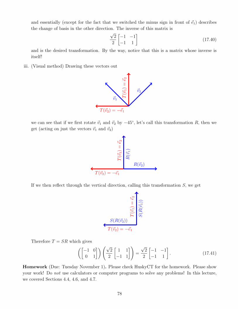
and essentially (except for the fact that we switched the minus sign in front of ~e1) describes

the change of basis in the other direction. The inverse of this matrix is√

2

2

[−1 −1

−1 1

](17.40)

and is the desired transformation. By the way, notice that this is a matrix whose inverse is

itself!

iii. (Visual method) Drawing these vectors out

T (~v2) = −~e1

T(~v

1)

=~e 2

~v1

~v2

we can see that if we first rotate ~v1 and ~v2 by −45, let’s call this transformation R, then we

get (acting on just the vectors ~v1 and ~v2)

T (~v2) = −~e1

T(~v

1)

=~e 2

R(~v

1)

R(~v2)

If we then reflect through the vertical direction, calling this transformation S, we get

T (~v2) = −~e1

T(~v

1)

=~e 2

S(R

(~v1))

S(R(~v2))

Therefore T = SR which gives([−1 0

0 1

])(√2

2

[1 1

−1 1

])=

√2

2

[−1 −1

−1 1

]. (17.41)

Homework (Due: Tuesday November 1). Please check HuskyCT for the homework. Please show


we covered Sections 4.4, 4.6, and 4.7.

78

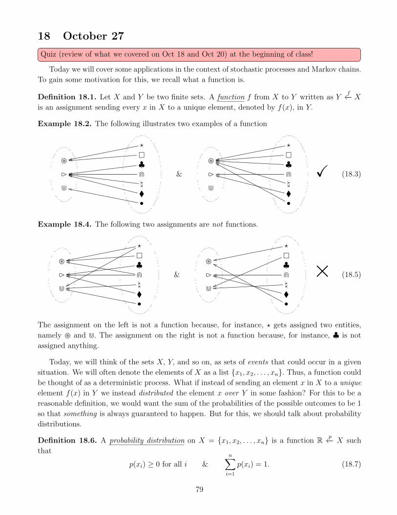
18 October 27

Quiz (review of what we covered on Oct 18 and Oct 20) at the beginning of class!

Today we will cover some applications in the context of stochastic processes and Markov chains.

To gain some motivation for this, we recall what a function is.

Definition 18.1. Let X and Y be two finite sets. A function f from X to Y written as Yf←− X

is an assignment sending every x in X to a unique element, denoted by f(x), in Y.

Example 18.2. The following illustrates two examples of a function

?

♣e\

•

3

d

rrpp

qqoommkk

ll

&

?

♣e\

•

3

d

rrppnn

oo

jj

kk

ff

X (18.3)

Example 18.4. The following two assignments are not functions.

?

♣e\

•

3

d

rrpp

xx

qq

ll

pp

ookk

ll

&

?

♣e\

•

3

d

rr

vv

oo

pp

kk

ff × (18.5)

The assignment on the left is not a function because, for instance, ? gets assigned two entities,

namely and d. The assignment on the right is not a function because, for instance, ♣ is not

assigned anything.

Today, we will think of the sets X, Y, and so on, as sets of events that could occur in a given

situation. We will often denote the elements of X as a list x1, x2, . . . , xn. Thus, a function could

be thought of as a deterministic process. What if instead of sending an element x in X to a unique

element f(x) in Y we instead distributed the element x over Y in some fashion? For this to be a

reasonable definition, we would want the sum of the probabilities of the possible outcomes to be 1

so that something is always guaranteed to happen. But for this, we should talk about probability

distributions.

Definition 18.6. A probability distribution on X = x1, x2, . . . , xn is a function R p←− X such

that

p(xi) ≥ 0 for all i &n∑i=1

p(xi) = 1. (18.7)

79

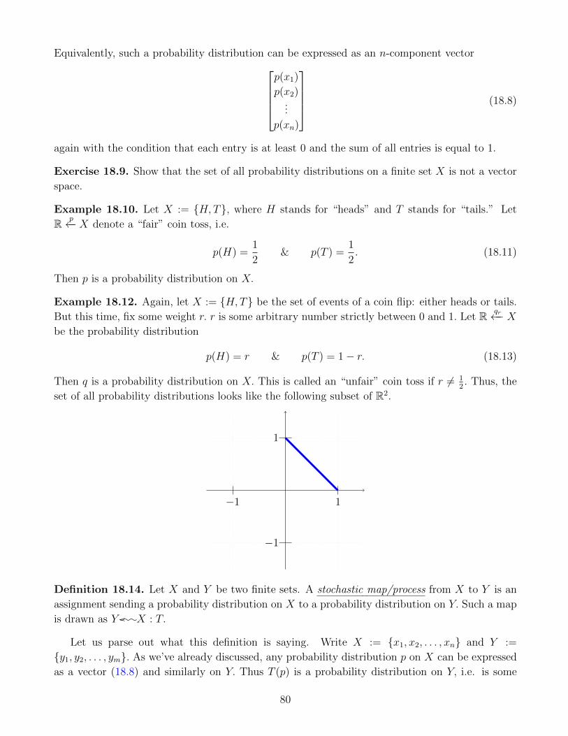
Equivalently, such a probability distribution can be expressed as an n-component vectorp(x1)

p(x2)...

p(xn)

(18.8)

again with the condition that each entry is at least 0 and the sum of all entries is equal to 1.

Exercise 18.9. Show that the set of all probability distributions on a finite set X is not a vector

space.

Example 18.10. Let X := H,T, where H stands for “heads” and T stands for “tails.” Let

R p←− X denote a “fair” coin toss, i.e.

p(H) =1

2& p(T ) =

1

2. (18.11)

Then p is a probability distribution on X.

Example 18.12. Again, let X := H,T be the set of events of a coin flip: either heads or tails.

But this time, fix some weight r. r is some arbitrary number strictly between 0 and 1. Let R qr←− X

be the probability distribution

p(H) = r & p(T ) = 1− r. (18.13)

Then q is a probability distribution on X. This is called an “unfair” coin toss if r 6= 12. Thus, the

set of all probability distributions looks like the following subset of R2.

−1 1

−1

1

Definition 18.14. Let X and Y be two finite sets. A stochastic map/process from X to Y is an

assignment sending a probability distribution on X to a probability distribution on Y. Such a map

is drawn as Y oo X : T.

Let us parse out what this definition is saying. Write X := x1, x2, . . . , xn and Y :=

y1, y2, . . . , ym. As we’ve already discussed, any probability distribution p on X can be expressed

as a vector (18.8) and similarly on Y. Thus T (p) is a probability distribution on Y, i.e. is some

80

vector (this time with m components). Is this starting to look familiar? T is an operation taking

an n-component vector to an m-component vector. It almost sounds as if T is described by some

matrix. Furthermore, we can look at the special probability distribution δxi defined by

δxi(xj) := δij :=

1 if i = j

0 otherwise(18.15)

(you may recognize this as the Kronecker-delta function). In other words, δxi describes the proba-

bility distribution that says the event xi will occur with %100 probability and no other event will

occur. As a vector, this looks like

δxi =

0...

0

1

0...

0

← i-th entry (18.16)

Therefore, we might expect that the probability distribution T (p) on Y is determined by the

probability distributions δxi since p itself can be written as a linear combination of these! Indeed,

we have

p =n∑i=1

p(xi)δxi , (18.17)

or in vector form p(x1)

p(x2)...

p(xn)

= p(x1)

1

0...

0

+ p(x2)

0

1...

0

+ · · ·+ p(xn)

0

0...

1

. (18.18)

Furthermore, whatever T is, it has to send the Kronecker-delta probability distribution to some

distribution on Y which is represented by an m-component vector

T (δxi) =:

T1i

T2i

...

Tmi

. (18.19)

The meaning of this vector is as follows. Imagine that the event xi takes place with %100 prob-

ability. Then the stochastic process says that after xi occurs, there is a T1i probability that the

event y1 will occur, a T2i probability that the event y2 will occur,..., and a Tmi probability that

the event ym will occur. This exactly describes the m-th column of a matrix. In other words, the

81

stochastic process is described by a matrix given by

T =

T11 T12 · · · T1n

T21 T22 · · · T2n

......

. . ....

Tm1 T2m · · · Tmn

(18.20)

where the i-th column represents physically the situation described in the past few sentences. Now

let’s go back to our initial probability distribution p on X. In this case, the event xi takes places

with probability p(xi) instead of %100. Given this information, what is the probability of the event

yj taking place after the stochastic process? This would be obtained by taking the j-th entry of

the resulting m-component vector from the matrix operationT11 T12 · · · T1n

T21 T22 · · · T2n

......

. . ....

Tm1 T2m · · · Tmn

p(x1)

p(x2)...

p(xn)

(18.21)

In other words,

yj =n∑i=1

Tjip(xi) (18.22)

is the probability of the event yj taking place given that the stochastic process T takes place and

the initial probability distribution on X was given by p.

Example 18.23. Imagine a machine that flips a coin and is programmed to always obtain heads

when given heads and always obtains tails when it is given tails. Unfortunately, machines are never

perfect and there are always subtle changes in the environment that actually make the probability

distribution slightly different. Oddly enough, the distribution for heads and tails was slightly

different after performing the tests over and over again. Given heads, the machine is %88 percent

likely to flip the coin and land heads again (leaving %12 for tails). Given tails, the machine is only

%86 likely to flip the coin and land tails again (leaving %14 for heads). The matrix associated to

this stochastic process is

T =

[0.88 0.14

0.12 0.86

]. (18.24)

Imagine I give the machine the coin heads up at first. After how many flips will the probability of

seeing heads be less than %65? After one flip, the probability of seeing heads is[0.88 0.14

0.12 0.86

] [1

0

]=

[0.88

0.12

](18.25)

as we could have guessed. After another turn, it becomes (after rounding and suppressing the

higher order terms) [0.88 0.14

0.12 0.86

] [0.88

0.12

]=

[0.79

.21

](18.26)

82

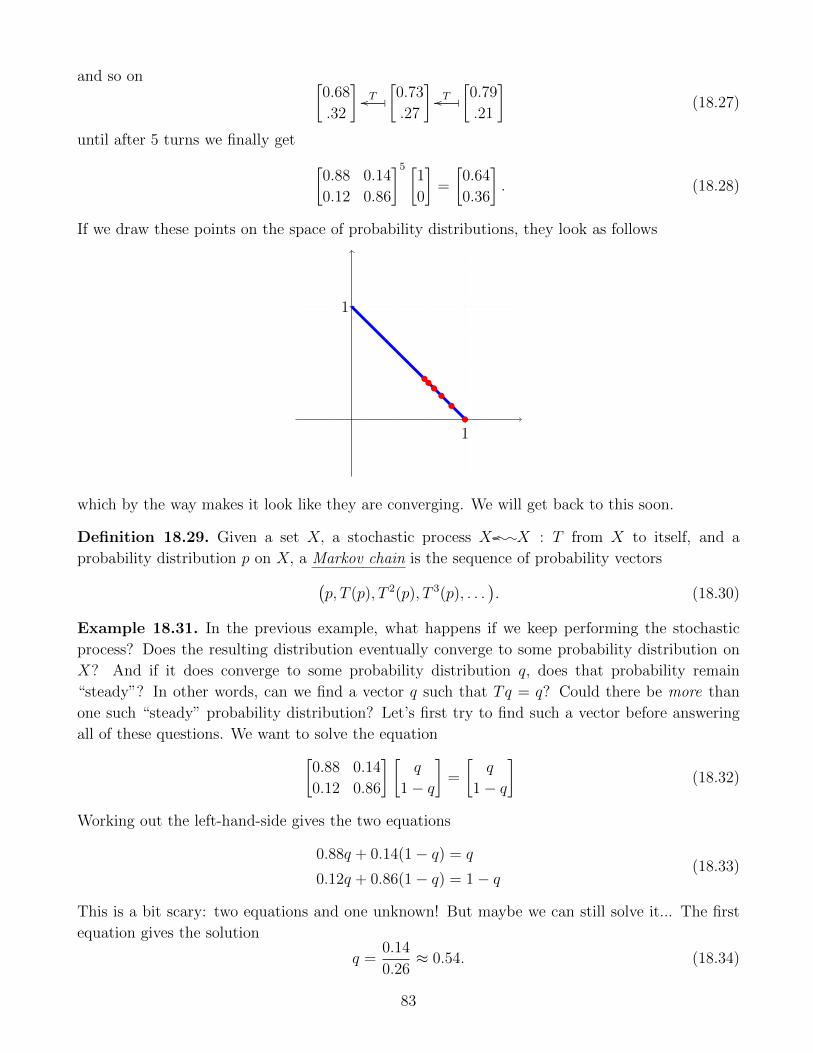
and so on [0.68

.32

]Too

[0.73

.27

]Too

[0.79

.21

](18.27)

until after 5 turns we finally get [0.88 0.14

0.12 0.86

]5 [1

0

]=

[0.64

0.36

]. (18.28)

If we draw these points on the space of probability distributions, they look as follows

1

1

•••

•••

which by the way makes it look like they are converging. We will get back to this soon.

Definition 18.29. Given a set X, a stochastic process X oo X : T from X to itself, and a

probability distribution p on X, a Markov chain is the sequence of probability vectors(p, T (p), T 2(p), T 3(p), . . .

). (18.30)

Example 18.31. In the previous example, what happens if we keep performing the stochastic

process? Does the resulting distribution eventually converge to some probability distribution on

X? And if it does converge to some probability distribution q, does that probability remain

“steady”? In other words, can we find a vector q such that Tq = q? Could there be more than

one such “steady” probability distribution? Let’s first try to find such a vector before answering

all of these questions. We want to solve the equation[0.88 0.14

0.12 0.86

] [q

1− q

]=

[q

1− q

](18.32)

Working out the left-hand-side gives the two equations

0.88q + 0.14(1− q) = q

0.12q + 0.86(1− q) = 1− q(18.33)

This is a bit scary: two equations and one unknown! But maybe we can still solve it... The first

equation gives the solution

q =0.14

0.26≈ 0.54. (18.34)

83

Fortunately, the second equation gives the same exact solution! What this is saying is that if I

was %54 sure that I gave the machine a coin with heads up, then the probability of the outcome

would be %54 heads every single time!

Definition 18.35. Let X be a set and T a stochastic process on X. A steady state probability

distribution for X and T is a probability distribution p on X such that T (p) = p.

A more clever way to solve for steady state probability distributions is to rewrite the equation

T (p) = p as (T − 1)(p) = 0, where 1 is the stochastic process that does nothing (in other words,

it leaves every single probability distribution alone). Since T − 1 can be represented as a matrix

and p as a vector, this amounts to solving a homogeneous system, which you are quite familiar

with by now. We now come to answering the many questions we had before.

Definition 18.36. Let X be a finite set. A T stochastic process on X is said to be regular if

there exists a positive integer k such that the matrix associated to T k has entries (T k)ij satisfying

0 < (T k)ij < 1 for all i and j.

Theorem 18.37. Let X be a finite set and T a regular stochastic process on X. Then, there exists

a unique probability distribution q on X such that T (q) = q. Furthermore, for any other probability

distribution p, the sequence (p, T (p), T 2(p), T 3(p), T 4(p), . . .

)(18.38)

converges to q.

We already saw this in the example above. We found a unique solution to the coin toss scenario

and we also observed how our initial configuration tended towards the steady state solution.



we covered parts of Sections 4.9 and my own personal notes.

84

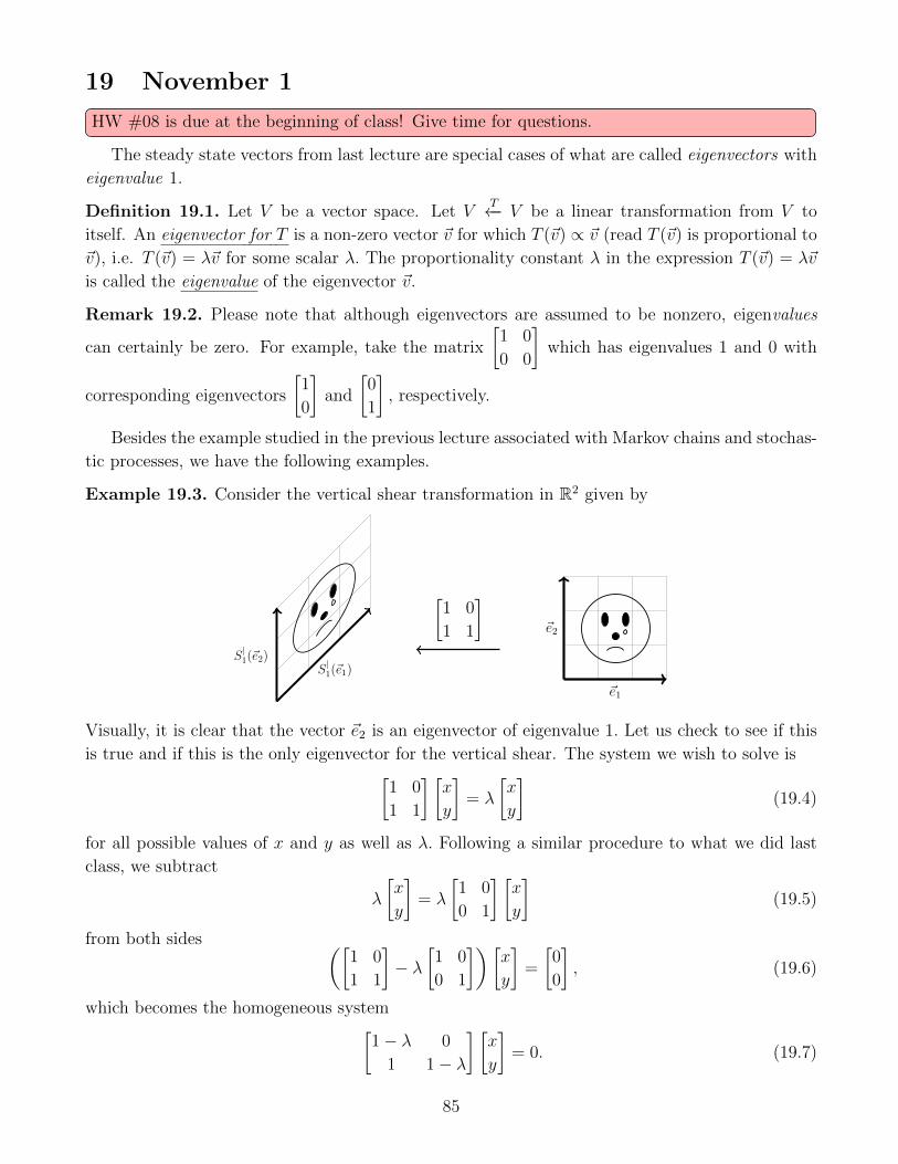
19 November 1


The steady state vectors from last lecture are special cases of what are called eigenvectors with

eigenvalue 1.

Definition 19.1. Let V be a vector space. Let VT←− V be a linear transformation from V to

itself. An eigenvector for T is a non-zero vector ~v for which T (~v) ∝ ~v (read T (~v) is proportional to

~v), i.e. T (~v) = λ~v for some scalar λ. The proportionality constant λ in the expression T (~v) = λ~v

is called the eigenvalue of the eigenvector ~v.

Remark 19.2. Please note that although eigenvectors are assumed to be nonzero, eigenvalues

can certainly be zero. For example, take the matrix

[1 0

0 0

]which has eigenvalues 1 and 0 with

corresponding eigenvectors

[1

0

]and

[0

1

], respectively.

Besides the example studied in the previous lecture associated with Markov chains and stochas-

tic processes, we have the following examples.

Example 19.3. Consider the vertical shear transformation in R2 given by

S|1(~e1)

S|1(~e2)

[1 0

1 1

]

~e1

~e2

Visually, it is clear that the vector ~e2 is an eigenvector of eigenvalue 1. Let us check to see if this

is true and if this is the only eigenvector for the vertical shear. The system we wish to solve is[1 0

1 1

] [x

y

]= λ

[x

y

](19.4)

for all possible values of x and y as well as λ. Following a similar procedure to what we did last

class, we subtract

λ

[x

y

]= λ

[1 0

0 1

] [x

y

](19.5)

from both sides ([1 0

1 1

]− λ

[1 0

0 1

])[x

y

]=

[0

0

], (19.6)

which becomes the homogeneous system[1− λ 0

1 1− λ

] [x

y

]= 0. (19.7)

85

Notice that we are trying to find a nontrivial solution to this system. Rather than trying to

manipulate these equations algebraically and solving these systems in a case by case basis, let us

analyze this system from the linear algebra perspective. Finding an eigenvector for the vertical

shear matrix amounts to finding a nontrivial solution to the system described by equation (19.7),

which means that the kernel of the matrix

[1− λ 0

1 1− λ

]must be nonzero, which, by the Invertible

Matrix Theorem, means the determinant of this matrix must be zero, i.e.

det

[1− λ 0

1 1− λ

]= 0. (19.8)

Solving this, we arrive at the polynomial equation

(1− λ)2 = 0. (19.9)

The only root of this polynomial is λ = 1 (in fact, λ = 1 appears twice, which means it has

multiplicity 2—more on this soon). Knowing this information, we can then solve the system (19.7)

much more easily since the equation reduces to[0 0

1 0

] [x

y

]= 0 (19.10)

and the set of solutions to this system is t

[0

1

], (19.11)

where t is a free variable. Therefore, all of the vectors of the form (19.11) are eigenvectors with

eigenvalue 1.

Example 19.12. Consider the rotation by angle π2

Rπ2(~e1)

Rπ2(~e2)

[0 −1

1 0

]

~e1

~e2

Following a similar procedure to the previous example, namely solving[0 −1

1 0

] [x

y

]= λ

[x

y

](19.13)

for all possible values of x and y as well as λ, we obtain[−λ −1

1 −λ

] [x

y

]=

[0

0

]. (19.14)

86

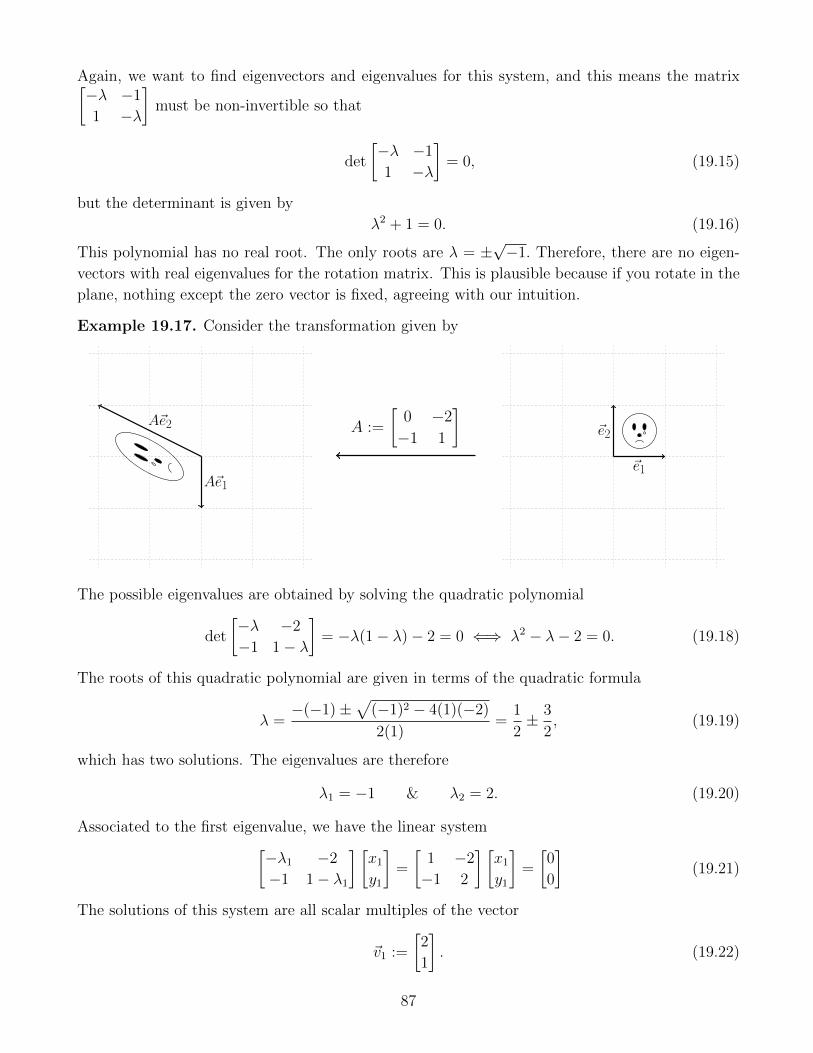
Again, we want to find eigenvectors and eigenvalues for this system, and this means the matrix[−λ −1

1 −λ

]must be non-invertible so that

det

[−λ −1

1 −λ

]= 0, (19.15)

but the determinant is given by

λ2 + 1 = 0. (19.16)

This polynomial has no real root. The only roots are λ = ±√−1. Therefore, there are no eigen-

vectors with real eigenvalues for the rotation matrix. This is plausible because if you rotate in the

plane, nothing except the zero vector is fixed, agreeing with our intuition.

Example 19.17. Consider the transformation given by

A~e1

A~e2 A :=

[0 −2

−1 1

]~e1

~e2

The possible eigenvalues are obtained by solving the quadratic polynomial

det

[−λ −2

−1 1− λ

]= −λ(1− λ)− 2 = 0 ⇐⇒ λ2 − λ− 2 = 0. (19.18)

The roots of this quadratic polynomial are given in terms of the quadratic formula

λ =−(−1)±

√(−1)2 − 4(1)(−2)

2(1)=

1

2± 3

2, (19.19)

which has two solutions. The eigenvalues are therefore

λ1 = −1 & λ2 = 2. (19.20)

Associated to the first eigenvalue, we have the linear system[−λ1 −2

−1 1− λ1

] [x1

y1

]=

[1 −2

−1 2

] [x1

y1

]=

[0

0

](19.21)

The solutions of this system are all scalar multiples of the vector

~v1 :=

[2

1

]. (19.22)

87

Therefore, ~v1 is an eigenvector of

[0 −2

−1 1

]with eigenvalue −1 because

[0 −2

−1 1

] [2

1

]= −1

[2

1

]. (19.23)

Similarly, associated to the second eigenvalue, we have the linear sytem[−λ2 −2

−1 1− λ2

] [x2

y2

]=

[−2 −2

−1 −1

] [x2

y2

]=

[0

0

](19.24)

whose solutions are all scalar multiples of the vector

~v2 :=

[1

−1

]. (19.25)

Again, this means that ~v2 is an eigenvector of

[0 −2

−1 1

]with eigenvalue 2 because

[0 −2

−1 1

] [1

−1

]= 2

[1

−1

]. (19.26)

Visually, under the transformation, these eigenvectors stay along the same line where they started

A~e1

A~e2

A~v1

A~v2

A :=

[0 −2

−1 1

]~e1

~e2 ~v1

~v2

The previous examples indicate the following general phenomena.

Theorem 19.27. Let A be an n× n matrix. The eigenvalues for the linear transformation asso-

ciated to A are given by the solutions to the polynomial equation

det (A− λ1n) = 0 (19.28)

in the variable λ.

Definition 19.29. For an n × n matrix A, the resulting polynomial det (A− λ1n) is called the

characteristic polynomial of A. If an eigenvalue appears k times as a root, then k is called the

multiplicity of that eigenvalue. The span of the eigenvectors of A for a particular eigenvalue λ is

called the eigenspace associated to A and λ.

88

An immediate consequence of the above theorem is the following.

Corollary 19.30. Let A be an upper-triangular n× n matrix of the form

A =

a11 a12 a13 · · · a1n

0 a22 a23 · · · a2n

0 0 a33 · · · a3n

.... . . . . .

...

0 0 · · · 0 ann

(19.31)

Then the eigenvalues of A are given by the roots of the polynomial

(a11 − λ)(a22 − λ)(a33 − λ) · · · (ann − λ) = 0. (19.32)

Another interesting fact that we did not point out explicitly from the examples but is also

visible is the following.

Theorem 19.33. Suppose that ~v1, . . . , ~vk are eigenvectors of a linear transformation VT←− V

with associated eigenvalues λ1, . . . , λk all of which are distinct. Then the set ~v1, . . . , ~vk is

linearly independent.

Proof.

Theorem 19.34. Let A be an n× n matrix. Let P be an invertible matrix and define

B := PAP−1. (19.35)

Then det(A) = det(B).

Proof. This follows immediately from the product rule for determinants, which says

det(B) = det(PAP−1) = det(P ) det(A) det(P−1) = det(P ) det(A) det(P )−1 = det(A). (19.36)

Definition 19.37. An n×n matrix A is similar to an n×n matrix B if there exists an invertible

n× n matrix P such that B = PAP−1.

Corollary 19.38. If an n×n matrix A is similar to an n×n matrix B, then the set of eigenvalues

of A is the same as the set of eigenvalues of B and their multiplicities will also be the same.

Remark 19.39. The converse of this corollary is not true! See your textbook for an example.



we covered Sections 5.1 and 5.2.

89

20 November 3

Quiz (review of what we covered on Oct 25 and Oct 27) at the beginning of class!

As we saw in the previous lecture, it is easy to compute the eigenvalues of an upper-triangular

matrix. It is equally simple to compute the eigenvalues of a diagonal matrix.

Definition 20.1. Let A be an n×n matrix. A is diagonalizable if it is similar to a diagonal matrix

D, i.e. if there exists an invertible n× n matrix P such that A = PDP−1.

Note that solving for D in the above equation gives D = P−1AP.

Theorem 20.2. An n× n matrix A is diagonalizable if and only if A has n linearly independent

eigenvectors. Furthermore, when A is diagonalizable and its eigenvectors are given by ~v1, . . . , ~vn,setting

P :=

~v1 · · · ~vn

, (20.3)

A can be expressed as

A = P

λ1 0 · · · 0

0 λ2...

.... . . 0

0 · · · 0 λn

P−1 (20.4)

where λi is the eigenvalue corresponding to the eigenvector ~vi, namely

A~vi = λi~vi (20.5)

for all i ∈ 1, . . . , n.

Example 20.6. Last class in Example 19.17, we found that the two eigenvalues with their corre-

sponding eigenvectors of the matrix

A :=

[0 −2

−1 1

](20.7)

are (λ1 = −1, ~v1 =

[2

1

])&

(λ2 = 2, ~v2 =

[1

−1

])(20.8)

As in Theorem 20.2, set

P :=

~v1 ~v2

=

[2 1

1 −1

](20.9)

from which we can calculate the inverse as

P−1 =1

3

[1 1

1 −2

]. (20.10)

90

We verify the claim of the theorem

PDP−1 =

[2 1

1 −1

] [−1 0

0 2

]1

3

[1 1

1 −2

]=

1

3

[2 1

1 −1

] [−1 −1

2 −4

]=

1

3

[0 −6

−3 3

]=

[0 −2

−1 1

]= A.

(20.11)

The following is a more complicated example but illustrates how to actually solve cubic poly-

nomials when calculating eigenvalues.

Example 20.12. Let A be the matrix34

A :=

0 1 1

2 1 2

3 3 2

. (20.13)

The eigenvalues of A are obtained from solving the polynomial equation

det(A− λ13) = det

−λ 1 1

2 1− λ 2

3 3 2− λ

= −λ det

[1− λ 2

3 2− λ

]− 1 det

[2 2

3 2− λ

]+ 1 det

[2 1− λ3 3

]= −λ

((1− λ)(2− λ)− 6

)−(

2(2− λ)− 6)

+(

6− 3(1− λ))

= −λ3 + 3λ2 + 9λ+ 5

= 0.

(20.14)

Solving cubic equations is not impossible, but it is difficult. A good strategy is to guess one solution

and then factor out that term to reduce it to a quadratic polynomial. By inspection, λ = −1 is

one such solution. Knowing this, we can use long division of polynomials

(λ+ 1) −λ3 + 3λ2 + 9λ+ 5

to figure out the other factors. To compute this division, one does what one is used to from

ordinary long division by calculating remainders

−λ2

(λ+ 1) −λ3 + 3λ2 + 9λ+ 5

−(−λ3 − λ2)

4λ2 + 9λ+ 5

34This is exercise 5.3.11 in [Lay] but without knowledge of any of the eigenvalues.

91

Proceeding, we get

−λ2 + 4λ

(λ+ 1) −λ3 + 3λ2 + 9λ+ 5

−(−λ3 − λ2)

4λ2 + 9λ+ 5

−(4λ2 + 4λ)

5λ+ 5

until finally

−λ2 + 4λ+ 5

(λ+ 1) −λ3 + 3λ2 + 9λ+ 5

−(−λ3 − λ2)

4λ2 + 9λ+ 5

−(4λ2 + 4λ)

5λ+ 5

−(5λ+ 5)

0

From this, we can factor our polynomial equation to the form

− λ3 + 3λ2 + 9λ+ 5 = (λ+ 1)(−λ2 + 4λ+ 5). (20.15)

Now we can apply the quadratic formula to find the roots of −λ2 + 4λ+ 5 and we get

λ =−4±

√42 − 4(−1)(5)

2(−1)= 2∓ 3. (20.16)

Thus, the polynomial factors into

− λ3 + 3λ2 + 9λ+ 5 = (λ+ 1)(λ+ 1)(−λ+ 5) = (λ+ 1)2(−λ+ 5) (20.17)

and the roots of the polynomial, i.e. the eigenvalues of the matrix A, are λ1 = −1, λ2 = −1, λ3 = 5.

Exercise 20.18. From Example 20.12, calculate the eigenvectors ~v1, ~v2, ~v3 of A associated to the

eigenvalues λ1, λ2, λ3, respectively. Construct the matrix P. Calculate P−1 and verify explicitly

that A = PDP−1.

Warning: not all matrices are diagonalizable.

Example 20.19. The vertical shear matrix

S|1 :=

[1 0

1 1

](20.20)

is not diagonalizable. One way to see this is to use Theorem 20.2. We have already calculated the

eigenvectors of this matrix in Example 19.3. We only found a single eigenvector[0

1

](20.21)

with eigenvalue 1. Since a single vector in R2 cannot span all of R2, this means there aren’t 2

linearly independent eigenvectors associated to this matrix. Therefore, S|1 is not diagonalizable.

92

Remark 20.22. Even though S|1 is not diagonalizable, it can be put into what is called Jordan

normal form, which is the next best thing after diagonal matrices. Namely, every matrix is similar

to a matrix of the form D + N, where D is diagonal and N has all zero entries except possibly

a few 1’s directly above the diagonal (and satisfies other properties). However, there is a caveat,

which is that one must allow for the matrices to be expressed in terms of complex numbers and

to allow for the diagonal matrix D to contain complex numbers as well.

Here’s a theorem that gives a sufficient condition for a matrix to be diagonalizable.

Theorem 20.23. Let A be an n×n matrix with n distinct eigenvalues. Then A is diagonalizable.

It is not necessary for a matrix A to have distinct eigenvalues to be diagonalizable. A simple

example is a matrix that is already in diagonal form. Once it is known that a matrix A is similar

to a diagonal matrix, it becomes easy to calculate “polynomials” in the matrix A. This is because

if P is an invertible matrix such that A = PDP−1, then

A2 =(PDP−1

)2= PDP−1P︸︷︷︸

=1n

DP−1 = PDDP−1 = PD2P−1 (20.24)

and similarly for higher orders

Ak =(PDP−1

)k= PDP−1P︸︷︷︸

=1n

DP−1P︸︷︷︸=1n

DP−1P︸︷︷︸=1n

DP−1 · · ·PDP−1 = PDkP−1. (20.25)

And to compute the power of a diagonal matrix is a piece of cake:λ1 0 · · · 0

0 λ2...

.... . . 0

0 · · · 0 λn

k

=

λk1 0 · · · 0

0 λk2...

.... . . 0

0 · · · 0 λkn

. (20.26)

Definition 20.27. Let A be an n× n matrix. Let p be a positive integer. A degree p polynomial

in A is an expression of the form

t01n + t1A+ t2A2 + · · ·+ tpA

p, (20.28)

where the t’s are real numbers.

Theorem 20.29. Let A be a diagonalizable n× n matrix with a decomposition of the form

A = PDP−1, (20.30)

where D is diagonalizable and P is a matrix of eigenvectors of A. Then

t01n + t1A+ t2A2 + · · ·+ tpA

p,= P(t01n + t1D + t2D

2 + · · ·+ tpDp)P−1. (20.31)



we covered Section 5.3.

93

21 November 8

Today we will review for the second midterm. Please look on HuksyCT for some sample problems.

Review quizzes, homework, suggested exercises, and class notes.

94

22 November 10

Today is the second midterm.

95

23 November 15


All the examples of eigenvalues and eigenvectors we mentioned were for n×nmatrices. However,

these concepts make sense for vectors spaces and linear transformations from a vector space to

itself.

Example 23.1. Consider the linear transformation nMnT←− nMn defined by sending an n × n

matrix A to T (A) := AT , the transpose of A. What are the eigenvalues and eigenvectors of

this transformation? Let us be concrete and analyze this problem for n = 2. Then, the linear

transformation acts as

T

([a b

c d

])=

[a c

b d

]. (23.2)

We want to find solutions, 2 × 2 matrices A, together with eigenvalues λ, satisfying T (A) = λA,

i.e. AT = λA. Right off the bat, we can guess three eigenvectors (remember, our vectors are now

2× 2 matrices!) by just looking at what T does in (23.2). These are

A1 =

[1 0

0 0

], A2 =

[0 0

0 1

], & A3 =

[0 1

1 0

]. (23.3)

Furthermore, their corresponding eigenvalues are all 1. This is because all of these matrices satisfy

ATi = Ai for i = 1, 2, 3. Is there a fourth eigenvector?35 For this, we could express the linear trans-

formation T in terms of the basis E := E11, E12, E21, E22. In this basis, the matrix representation

of T is given by

[T ]E =

1 0 0 0

0 0 1 0

0 1 0 0

0 0 0 1

E

(23.4)

because

T (E11) = E11

T (E12) = E21

T (E21) = E12

T (E22) = E22.

(23.5)

35We do not have to go through this entire calculation that follows to find this fourth eigenvector. One can think

about what it should be by guessing, but we will go through this to illustrate what one would do even if it is not

apparent.

96

The characteristic polynomial associated to this transformation is

det

1− λ 0 0 0

0 −λ 1 0

0 1 −λ 0

0 0 0 1− λ

= (1− λ) det

−λ 1 0

1 −λ 0

0 0 1− λ

= (1− λ)2 det

[−λ 1

1 −λ

]= (1− λ)2(λ2 − 1)

= (1− λ)3(λ+ 1).

(23.6)

Hence, we see that there is another eigenvalue, namely, λ4 = −1. The corresponding eigenvector

can be solved for by solving the linear system2 0 0 0 0

0 1 1 0 0

0 1 1 0 0

0 0 0 2 0

→

1 0 0 0 0

0 1 1 0 0

0 0 0 0 0

0 0 0 1 0

(23.7)

whose solutions are all of the form

s

0

−1

1

0

E

(23.8)

with s a free variable, which in terms of 2× 2 matrices is given by

s

[0 −1

1 0

]. (23.9)

Hence, our fourth eigenvector for T can be taken to be

A4 =

[0 −1

1 0

](23.10)

and its corresponding eigenvalue is λ4 = −1.

Example 23.11. Consider the following two bases of degree 2 polynomials

q0(x) = 0 + 2x+ 3x2 p0(x) = 1

q1(x) = 1 + 1x+ 3x2 p1(x) = x

q2(x) = 1 + 2x+ 2x2 p2(x) = x2

and the linear transformation P2T←− P2 satisfying T (pi) = qi for i = 0, 1, 2. A matrix representation

of this transformation in the P := p0, p1, p2 basis is given by

[T ]P =

0 1 1

2 1 2

3 3 2

P

. (23.12)

97

Because this matrix has nonzero determinant (detT = 5), it is invertible. In fact, we studied this

matrix in Example 20.12. A matrix representation of the inverse of this transformation is given in

the Q := q0, q1, q2 basis by

[T−1]Q =1

5

−4 1 1

2 −3 2

3 3 −2

Q

. (23.13)

and satisfies T−1(qi) = pi for i = 0, 1, 2. To check this, let us make sure that the first column of

this matrix expresses the polynomial p0 in the Q basis.

−4

5q0(x) +

2

5q1(x) +

3

5q2(x) = −4

5(0 + 2x+ 3x2)

+2

5(1− 1x+ 3x2)

− 3

5(1 + 2x+ 2x2)

= 1(1 + 0x+ 0x2)

= p0(x).

Anyway, we’d like to find the eigenvalues and corresponding eigenvectors of T . To do this, we

can use any basis we’d like and use the matrix representation of T in this basis. Therefore,

we can simply find the roots of the characteristic polynomial, which we have already done in

Example 20.12. They were λ1 = −1, λ2 = −1, λ3 = 5. We should now calculate the corresponding

eigenvectors. For λ1 = λ2 = −1, we have to solve1 1 1 0

2 2 2 0

3 3 3 0

→1 1 1 0

0 0 0 0

0 0 0 0

(23.14)

which has solutions

y

−1

1

0

P

+ z

−1

0

1

P

(23.15)

with two free variables y and z. Hence, a basis for such solutions, and therefore two eigenvectors

for λ1 and λ2, is given by the two vectors

~v1 =

−1

1

0

P

& ~v2 =

−1

0

1

P

. (23.16)

(Note: your choice of eigenvectors could be different from mine!) For the eigenvalue λ3 = 5, we

must solve−5 1 1 0

2 −4 2 0

3 3 −3 0

→0 0 0 0

1 −2 1 0

1 1 −1 0

→0 0 0 0

1 −2 1 0

0 3 −2 0

→0 0 0 0

1 0 −1/3 0

0 1 −2/3 0

(23.17)

98

which has solutions

z

1/3

2/3

1

P

(23.18)

with z a free variable. Thus, an eigenvector for λ3 is

~v3 =

1

2

3

P

. (23.19)

In terms of the polynomials, the eigenvalues together with their corresponding eigenvectors in P2

are given by

λ1 ↔ −p0 + p1 ↔ −1 + x

λ2 ↔ −p0 + p2 ↔ −1 + x2

λ3 ↔ p0 + 2p1 + 3p2 ↔ 1 + 2x+ 3x2

(23.20)

As we saw in earlier lectures, some n × n matrices do not have n eigenvalues or a basis of

n eigenvectors. For example, shears in two dimensions only have a one-dimensional basis of

eigenvectors and rotations in two dimensions have none! Each of these problems has a resolution,

the former in terms of what are called generalized eigenvectors, and the latter in terms of complex

eigenvectors. The former is typically studied in a more advanced course on linear algebra (such as

the one being offered next semester).

Definition 23.21. A complex number is an ordered pair of real numbers (a, b) with a, b both real

together with the following addition and multiplication operations. Addition is defined component-

wise

(a, b) + (c, d) := (a+ c, b+ d) (23.22)

and multiplication is defined by36

(a, b)(c, d) := (ac− bd, ad+ bc) (23.23)

for all real numbers a, b, c, d. Define√−1 to be

√−1 := (0, 1). (23.24)

Notice that 1 := (1, 0) is good notation for the unit under multiplication because

1(a, b) ≡ (1, 0)(a, b) = (a, b) (23.25)

and similarly on the right. Here the ≡ symbol means “equivalent” and is just relating the two

possible notations for complex numbers. In fact, using the definition of the expression√−1 and

1, it is common to write

(a, b) ≡ a+ b√−1 (23.26)

36Warning! This is not the “dot product”! We have not talked about the dot product, but we will next lecture,

and the two are very different. We will actually use a different notation to avoid possible confusion between dots

and multiplication.

99

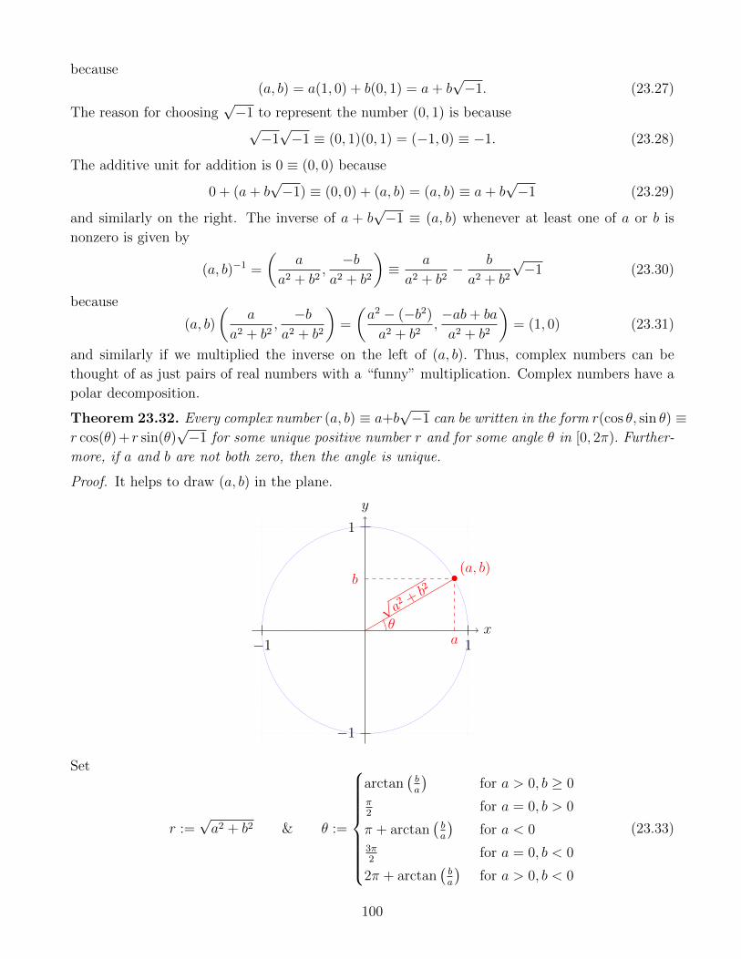
because

(a, b) = a(1, 0) + b(0, 1) = a+ b√−1. (23.27)

The reason for choosing√−1 to represent the number (0, 1) is because√−1√−1 ≡ (0, 1)(0, 1) = (−1, 0) ≡ −1. (23.28)

The additive unit for addition is 0 ≡ (0, 0) because

0 + (a+ b√−1) ≡ (0, 0) + (a, b) = (a, b) ≡ a+ b

√−1 (23.29)

and similarly on the right. The inverse of a + b√−1 ≡ (a, b) whenever at least one of a or b is

nonzero is given by

(a, b)−1 =

(a

a2 + b2,−b

a2 + b2

)≡ a

a2 + b2− b

a2 + b2

√−1 (23.30)

because

(a, b)

(a

a2 + b2,−b

a2 + b2

)=

(a2 − (−b2)

a2 + b2,−ab+ ba

a2 + b2

)= (1, 0) (23.31)

and similarly if we multiplied the inverse on the left of (a, b). Thus, complex numbers can be

thought of as just pairs of real numbers with a “funny” multiplication. Complex numbers have a

polar decomposition.

Theorem 23.32. Every complex number (a, b) ≡ a+b√−1 can be written in the form r(cos θ, sin θ) ≡

r cos(θ) + r sin(θ)√−1 for some unique positive number r and for some angle θ in [0, 2π). Further-

more, if a and b are not both zero, then the angle is unique.

Proof. It helps to draw (a, b) in the plane.

x

y

−1 1

−1

1

•b

a

(a, b)

√ a2 + b

2

θ

Set

r :=√a2 + b2 & θ :=

arctan(ba

)for a > 0, b ≥ 0

π2

for a = 0, b > 0

π + arctan(ba

)for a < 0

3π2

for a = 0, b < 0

2π + arctan(ba

)for a > 0, b < 0

(23.33)

100

where θ is defined as long as both a and b are not zero. If a = b = 0, θ can be anything. Visually,

the function θ can be drawn as a (discontinuous) function on the circle.37

y

z

x

Let’s get back to linear algebra now and analyze the rotation in two dimensions.

Example 23.34. As we saw in Example 19.12, the characteristic polynomial associated to the

rotation by angle π2

matrix given by

Rπ2

:=

[0 −1

1 0

](23.35)

is

λ2 + 1 = 0. (23.36)

Using just real numbers, no such solution exists. However, using complex numbers, we know

exactly what λ should be. The possible choices are

λ1 =√−1 & λ2 = −

√−1 (23.37)

since both satisfy λ2 = −1. What are the corresponding eigenvectors? As usual, we solve a

homogeneous problem for each eigenvalue. For λ1, we have[−√−1 −1 0

1 −√−1 0

]→[−1

√−1 0

1 −√−1 0

]→[1 −

√−1 0

0 0 0

](23.38)

37The code for this cylinder is modified from code written by Gonzalo Medina http://tex.stackexchange.com/

questions/255485/tikz-drawing-a-cylinder-with-a-hole-the-bottom.

101

http://tex.stackexchange.com/questions/255485/tikz-drawing-a-cylinder-with-a-hole-the-bottom

http://tex.stackexchange.com/questions/255485/tikz-drawing-a-cylinder-with-a-hole-the-bottom

which has solutions of the form

t

[−√−1

1

](23.39)

with t a free variable. Hence one such eigenvector for λ1 is

~v1 =

[1√−1

](23.40)

(I multiplied throughout by√−1 so that the first entry is a 1). Similarly, for λ2 one finds that

one such eigenvector is

~v2 =

[1

−√−1

]. (23.41)

Hence, the rotation matrix does have eigenvalues and eigenvectors—we just can’t see them!

Exercise 23.42. Show that the eigenvalues of a matrix of the form[a −bb a

](23.43)

are of the form

a± b√−1. (23.44)

Complex eigenvalues and eigenvectors can be interpreted in this way as types of rotations in a

particular plane. Hence, they always come in pairs.

Definition 23.45. Let (a, b) ≡ a+ b√−1 be a complex number (a and b are real numbers). The

complex conjugate of (a, b) ≡ a+ b√−1 is

(a, b) = (a,−b) (23.46)

or in terms of the notation a+ b√−1 this is written as

a+ b√−1 = a− b

√−1. (23.47)

Definition 23.48. Let Cn be the vector space of n-component vectors but whose entries are all

complex numbers. Addition, scalar multiplication (this time using complex numbers!), and the

zero vector are analogous to how they are defined for Rn. Similarly, m× n matrices can be taken

to have complex numbers as their entries and are (complex) linear transformations Rm ← Rn.

Theorem 23.49. Let A be an n× n matrix with complex entries. If λ is an eigenvalue of A then

λ is also an eigenvalue.

Theorem 23.50. Let A be an n × n matrix with complex entries. Then A has n (complex)

eigenvalues including mutiplicity.




102

24 November 17

Quiz (review of what we covered on Nov 1 and Nov 3) at the beginning of class! Know how to

find eigenvectors and eigenvalues for 3 × 3 matrices and also how to diagonalize 3 × 3 matrices

(when it is possible).

Last class we talked about complex numbers and how every complex number can be expressed

in terms of its magnitude and a direction. The abstract notion of the Euclidean inner product in

Rn provides generalizations of several familiar concepts such as the magnitude of any vector, the

length between two points (vectors), the projection of one vector onto a line, and so on.

Definition 24.1. Let ~v and ~u be two vectors in Rn with components written out as

~v =

v1

v2

...

vn

& ~u =

u1

u2

...

un

. (24.2)

The Euclidean inner product of ~u with ~v (referred to as the dot product in your book) is the real

number

〈~u,~v〉 := u1v1 + u2v2 + · · ·+ unvn. (24.3)

The notion of length is a special case of the Euclidean inner product.

Definition 24.4. Let ~v be a vector in Rn with components written out as

~v =

v1

v2

...

vn

. (24.5)

The length of ~v is

‖~v‖ :=√〈~v,~v〉 =

√v2

1 + v22 + · · ·+ v2

n. (24.6)

v2

v1

(v1, v2)

√ v21+ v

22

103

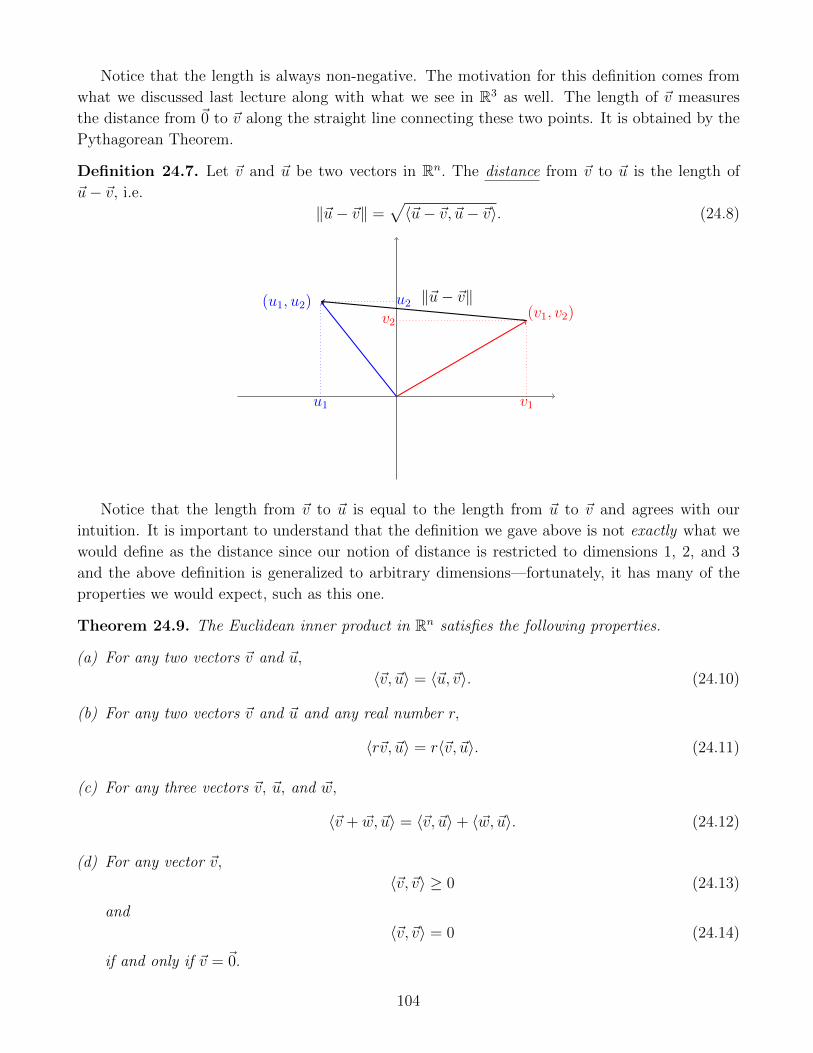
Notice that the length is always non-negative. The motivation for this definition comes from

what we discussed last lecture along with what we see in R3 as well. The length of ~v measures

the distance from ~0 to ~v along the straight line connecting these two points. It is obtained by the

Pythagorean Theorem.

Definition 24.7. Let ~v and ~u be two vectors in Rn. The distance from ~v to ~u is the length of

~u− ~v, i.e.

‖~u− ~v‖ =√〈~u− ~v, ~u− ~v〉. (24.8)

v2

v1

(v1, v2)u2

u1

(u1, u2) ‖~u− ~v‖

Notice that the length from ~v to ~u is equal to the length from ~u to ~v and agrees with our

intuition. It is important to understand that the definition we gave above is not exactly what we

would define as the distance since our notion of distance is restricted to dimensions 1, 2, and 3

and the above definition is generalized to arbitrary dimensions—fortunately, it has many of the

properties we would expect, such as this one.

Theorem 24.9. The Euclidean inner product in Rn satisfies the following properties.

(a) For any two vectors ~v and ~u,

〈~v, ~u〉 = 〈~u,~v〉. (24.10)

(b) For any two vectors ~v and ~u and any real number r,

〈r~v, ~u〉 = r〈~v, ~u〉. (24.11)

(c) For any three vectors ~v, ~u, and ~w,

〈~v + ~w, ~u〉 = 〈~v, ~u〉+ 〈~w, ~u〉. (24.12)

(d) For any vector ~v,

〈~v,~v〉 ≥ 0 (24.13)

and

〈~v,~v〉 = 0 (24.14)

if and only if ~v = ~0.

104

Proof. space

(a) Because multiplication of numbers is commutative

〈~v, ~u〉 = v1u1 + v2u2 + · · ·+ vnun = u1v1 + u2v2 + · · ·+ unvn = 〈~u,~v〉. (24.15)

(b) Because multiplication of real numbers is associative and distributive over addition

〈r~v, ~u〉 = (rv1)u1 + (rv2)u2 + · · ·+ (rvn)un

= r(v1u1) + r(v2u2) + · · ·+ r(vnun)

= r(v1u1 + v2u2 + · · ·+ vnun)

= r〈~v, ~u〉.

(24.16)

(c) By the distributive law and commutativity (and associativity of addition)

〈~v + ~w, ~u〉 = (v1 + w1)u1 + (v2 + w2)u2 + · · ·+ (vn + wn)un

= v1u1 + w1u1 + v2u2 + w2u2 + · · ·+ vnun + wnun

= v1u1 + v2u2 + · · ·+ vnun + w1u1 + w2u2 + · · ·+ wnun

= 〈~v, ~u〉+ 〈~w, ~u〉.

(24.17)

(d) For any vector ~v,

〈~v,~v〉 = v21 + v2

2 + · · ·+ v2n ≥ 0 (24.18)

because each term is non-negative since the square of any real number is non-negative. Fur-

thermore, this quantity is zero if and only if every term is zero, which holds if and only if

~v = ~0.

We can also use the inner product to define angles between vectors.

Definition 24.19. Let ~v and ~u be two nonzero vectors in Rn. The angle θ from ~v to ~u

θ := arccos

(〈~v, ~u〉‖~v‖‖~u‖

). (24.20)

Again, this definition is motivated by what we are used to in low dimensions and follows from

the law of cosines

b := ‖~v‖a := ‖~u‖θ

c := ‖~u− ~v‖

105

which says

c2 = a2 + b2 − 2ab cos(θ). (24.21)

In terms of the Euclidean inner product and the vectors ~u and ~v, this reads

〈~u− ~v, ~u− ~v〉 = 〈~u, ~u〉+ 〈~u, ~u〉 − 2‖~u‖‖~v‖ cos(θ). (24.22)

The left-hand-side of (24.22) reduces to

〈~u− ~v, ~u− ~v〉 = 〈~u− ~v, ~u〉 − 〈~u− ~v,~v〉 = 〈~u, ~u〉 − 2〈~u,~v〉+ 〈~v,~v〉 (24.23)

by parts (a), (b), and (c) of Theorem 24.9. Two of these terms cancel from equation (24.22) giving

− 2〈~u,~v〉 = −2‖~u‖‖~v‖ cos(θ), (24.24)

which reproduces the formula for the angle θ.

A closely related concept to distance and length is that of a projection of one vector onto

another. For this we need the notion of a unit vector.

Definition 24.25. A vector ~u in Rn of length 1 is called a normalized/unit vector. If ~v is any

nonzero vector in Rn, its normalization is given by38

~v

‖~v‖. (24.26)

~v~v‖~v‖

~v~v‖~v‖

Definition 24.27. Let ~v and ~u be two vectors in Rn. The vector projection of ~v onto ~u is the

vector ~v|~u given by

~v|~u :=

(〈~v, ~u〉‖~u‖

)~u

‖~u‖. (24.28)

The scalar projection of ~v onto ~u is the Euclidean inner product of the vector projection of ~v onto

~u with ~u‖~u‖ ⟨

~v|~u,~u

‖~u‖

⟩=〈~v, ~u〉‖~u‖

. (24.29)

38The sphere drawing was done using a modified version of code written by Christian Feuersanger and was found

at http://tex.stackexchange.com/questions/124916/draw-sphere-pgfplots-with-axis-at-center.

106

http://tex.stackexchange.com/questions/124916/draw-sphere-pgfplots-with-axis-at-center

Definition 24.30. Two vectors ~u and ~v are orthogonal whenever 〈~v, ~u〉 = 0.

In terms of the definition of angle, this says that the angle between ~v and ~u is an odd integer

multiple of π2, as we would expect from our common-day use of the word orthogonal.

Definition 24.31. Let ~v be a nonzero vector in Rn and let L := span~v. The orthogonal

complement of L is

L⊥ :=~u ∈ Rn : 〈~v, ~u〉 = 0

(24.32)

i.e. the set of vectors ~u in Rn that are orthogonal to ~v.

Example 24.33. Consider the vector

~v :=

[1

2

](24.34)

in R2 and let L := span~v. Then

L⊥ =aRπ

2(~v) : a ∈ R

, (24.35)

where Rπ2

is the 2× 2 rotation matrix, is the set of all scalar multiples of the vector ~v after it has

been rotated by 90. More explicitly,

L⊥ = span

[−2

1

](24.36)

~v

LL⊥

Example 24.37. Consider the vector

~v :=

1

2

3

(24.38)

in R3 and let L := span~v. Then

L⊥ =

xyz

∈ R3 :

⟨3

2

1

,xyz

⟩ = 0

=

xyz

∈ R3 : 3x+ 2y + z = 0

(24.39)

107

which describes the plane z = −3x− 2y. In other words,

L⊥ =

x 1

0

−3

+ y

0

1

−2

∈ R3 : x, y ∈ R

= span

1

0

−3

, 0

1

−2

.

(24.40)

More generally, we can define the orthogonal complement of any subspace.

Definition 24.41. Let W be a k-dimensional subspace of Rn. The orthogonal complement of W

is

W⊥ :=~u ∈ Rn : 〈~v, ~u〉 = 0 for all ~v ∈ W

(24.42)

i.e. the set of vectors ~u in Rn that are orthogonal to all vectors ~v in W.

Example 24.43. The orthogonal complement of the plane P described by the equation z =

−3x− 2y is precisely the one-dimensional subspace L from Example 24.33 because

P⊥ =

v1

v2

v3

∈ R3 :

⟨v1

v2

v3

, x 1

0

−3

+ y

0

1

−2

⟩ = 0 for all x, y ∈ R

=

v1

v2

v3

∈ R3 : v1x+ v2y − (3x+ 2y)v3 = 0 for all x, y ∈ R

=

v1

v2

v3

∈ R3 : x(v1 − 3v3) + y(v2 − 2v3) = 0 for all x, y ∈ R

=

v1

v2

v3

∈ R3 : v1 = 3v3 and v2 = 2v3

= span

3

2

1

.

(24.44)

This phenomenon of taking the orthogonal complement twice to get back what you started is

true in general.

Theorem 24.45. Let W be a k-dimensional subspace of Rn. Then the orthogonal complement

W⊥ is an (n − k)-dimensional subspace of Rn. Furthermore, the orthogonal complement of the

orthogonal complement is the original subspace itself, i.e.

(W⊥)⊥ = W. (24.46)

108

We can use the properties from Theorem 24.9 to define the notion of an inner product in any

vector space.

Definition 24.47. Let V be a vector space. An inner product on V is a function

〈 · , · 〉 : V × V → R, (24.48)

taking two vectors and producing a real number, satisfying the following axioms.

(a) For any two vectors ~v and ~u in V,

〈~v, ~u〉 = 〈~u,~v〉. (24.49)

(b) For any two vectors ~v and ~u in V and any real number r,

〈~v, r~u〉 = r〈~v, ~u〉. (24.50)

(c) For any three vectors ~v, ~u, and ~w in V,

〈~v + ~w, ~u〉 = 〈~v, ~u〉+ 〈~w, ~u〉. (24.51)

(d) For any vector ~v in V,

〈~v,~v〉 ≥ 0 (24.52)

and

〈~v,~v〉 = 0 (24.53)

if and only if ~v = ~0.

A vector space together with an inner product is called an inner product space.

With this definition we can talk about many fascinating examples of inner products. Just as

we defined the length of a vector, unit vectors, distance between vectors, angles, projections, and

perpendicular subspaces in Rn, we can make completely analogous definitions for inner product

spaces (if you look back, all of these definitions only depended on the inner product!).

Theorem 24.54 (Cauchy-Schwarz). Let V be an inner product space. For all vectors ~u and ~v in

V, ∣∣〈~v, ~u〉∣∣ ≤ ‖~u‖‖~v‖. (24.55)

Theorem 24.56 (Triangle Inequality). Let V be an inner product space. For all vectors ~u and ~v

in V,

‖~u+ ~v‖ ≤ ‖~u‖+ ‖~v‖. (24.57)




109

25 November 29


Theorem 25.1. Let V be a finite-dimensional vector space with an inner product 〈 · , · 〉 let W

be a subspace of V, and let ~v be a vector in V. Then there exist unique vectors ~w in W ~u in W⊥

satisfying ~v = ~w + ~u.

Before proving this theorem, we will go through some definitions and properties of orthogonal-

ity.

Definition 25.2. Let V be a vector space with an inner product 〈 · , · 〉. A set S := ~v1, ~v2, . . . , ~vnof vectors in V is an orthogonal set iff 〈~vi, ~vj〉 = 0 whenever i 6= j. If, in addition, ‖~vi‖ = 1 for all

i = 1, 2, . . . , n, then S is an orthonormal set of vectors in V.

From the examples of the last class, we noticed some interesting properties of sets of orthogonal

vectors when studying the orthogonal complement.

Theorem 25.3. Let V be a vector space with an inner product 〈 · , · 〉 and let S := ~v1, ~v2, . . . , ~vnbe an orthogonal set in V of non-zero vectors. Then S is linearly independent. In particular, S is

a basis for span(S).

Proof. See Lay.

Given an orthogonal set ~v1, ~v2, . . . , ~vn of nonzero vectors in V, the set~v1

‖~v1‖,~v2

‖~v2‖, . . . ,

~vn‖~vn‖

,

(25.4)

is an orthonormal set. An orthonormal set of vectors in V has many similar properties to the

vectors ~e1, ~e2, · · · , ~em in Rn, where m ≤ n.

Theorem 25.5. Let V be a vector space with an inner product 〈 · , · 〉, let S := ~u1, ~u2, . . . , ~unbe an orthonormal set in V, and let ~v be a vector in span(S). Then

~v = 〈~v, ~u1〉~u1 + 〈~v, ~u2〉~u2 + · · ·+ 〈~v, ~un〉~un. (25.6)

Furthermore, since S is a basis for span(S), these linear combinations are unique.

We will prove this theorem more generally shortly. But what happens if ~v is not in the subspace

spanned by an orthonormal set? The following theorem answers this question.

Theorem 25.7. Let V be a vector space with an inner product 〈 · , · 〉, let S := ~u1, ~u2, . . . , ~unbe an orthonormal set in V, and let ~v be a vector in V. Then there exists a unique decomposition

~v = 〈~v, ~u1〉~u1 + 〈~v, ~u2〉~u2 + · · ·+ 〈~v, ~un〉~un + ~v⊥, (25.8)

where

~v⊥ := ~v −(〈~v, ~u1〉~u1 + 〈~v, ~u2〉~u2 + · · ·+ 〈~v, ~un〉~un

)(25.9)

110

is in span(S)⊥. In fact, the transformation VPW←−− V defined by sending ~v in V to

PW (~v) := 〈~v, ~u1〉~u1 + 〈~v, ~u2〉~u2 + · · ·+ 〈~v, ~un〉~un (25.10)

is a linear transformation satisfying

P 2W = PW . (25.11)

Proof. The first thing we check is that ~v⊥ is in span(S)⊥. For this, notice that

〈~v⊥, ~ui〉 =⟨~v −

(〈~v, ~u1〉~u1 + 〈~v, ~u2〉~u2 + · · ·+ 〈~v, ~un〉~un

), ~ui

⟩= 〈~v, ~ui〉 −

n∑j=1

〈~v, ~uj〉〈~uj, ~ui〉

= 〈~v, ~ui〉 −n∑j=1

〈~v, ~uj〉δji

= 〈~v, ~ui〉 − 〈~v, ~ui〉= 0.

(25.12)

Since this is true for every i = 1, 2, . . . , n, it follows that 〈~v⊥, ~u〉 = 0 for every vector ~u in span(S),

since every such vector is expressed as a linear combination of these elements in S. Hence, ~v⊥ is

in span(S)⊥.

The second thing we check is that P 2W = PW (it is not difficult to see that PW is in fact a linear

transformation). For this, let ~v be a vector in V and calculating P 2W (~v) gives

P 2W (~v) = PW

(n∑i=1

〈~v, ~ui〉~ui

)

=n∑i=1

(〈~v, ~ui〉PW (~ui)

)=

n∑i=1

(〈~v, ~ui〉

n∑j=1

〈~ui, ~uj〉~uj

)

=n∑i=1

(〈~v, ~ui〉

n∑j=1

δij~uj

)

=n∑i=1

(〈~v, ~ui〉~ui

)= PW (~v)

(25.13)

as needed.

The last condition in Theorem 25.7 is what defines a projection.

Definition 25.14. Let V be a finite-dimensional vector space. A linear transformation VT←− V

is a projection whenever T 2 = T.

111

A nice way to think about projections is given at http://math.stackexchange.com/questions/

1303977/what-is-the-idea-behind-a-projection-operator-what-does-it-do.

The only difference between Theorem 25.7 and Theorem 25.1 is that Theorem 25.1 only assumes

the presence of a subspace W but not necessarily an orthonormal set spanning W as in Theorem

25.7. There is a subtle, but importance difference between these two hypotheses. Indeed, given an

arbitrary subspace W, how do we know if a orthonormal set spanning W even exists? We know

a basis always exists, but a basis is quite different from an orthonormal set (not every basis is an

orthonormal set but every orthonormal set is a basis for the space it spans). The Gram-Schmidt

process, a process we are about to describe, provides a construction of an orthonormal set for any

subspace of a finite-dimensional inner product space. Hence, not only does it prove the existence

of an orthonormal set for a subspace, it provides a step-by-step procedure for producing one!

Construction 25.15 (The Gram-Schmidt Process). Let V be a finite-dimensional inner product

space and let W be a nonzero subspace. Because V is finite-dimensional, W is finite-dimensional.

Hence, there exists a basis B := ~w1, ~w2, . . . , ~wn, with n ≥ 1, for W. Set

~u1 :=~w1

‖~w1‖(25.16)

and let W1 := span(~w1) ≡ span(~u1). Set

~v2 := ~w2 − 〈~w2, ~u1〉~u1, (25.17)

i.e. the component of ~w2 perpendicular to W1. Normalize it by setting

~u2 :=~v2

‖~v2‖(25.18)

and set W2 := span(~u1, ~u2

). Proceed inductively. Namely, suppose that ~um and Wm have been

constructed and 1 < m < n. Then, set

~vm+1 := ~wm+1 −m∑i=1

〈~wm+1, ~ui〉~ui, (25.19)

i.e. the component of ~wm+1 perpendicular to Wm. Normalize it by setting

~um+1 :=~vm+1

‖~vm+1‖(25.20)

and set Wm+1 := span(~u1, ~u2, . . . , ~um+1

). After this construction is done (which must happen

since n is finite), the set S := ~u1, ~u2, . . . , ~un of vectors has been constructed along with a sequence

of subspaces W1,W2, . . . ,Wn satisfying the following properties.

(a) The set S is orthonormal.

(b) Wn = W. In fact, span(S) = W.

The first claim follows from the construction. The second claim follows from the fact that S is a

basis of Wn containing n elements, but Wn is a subspace of W, which also has a basis containing

n elements, which implies W = Wn.

112

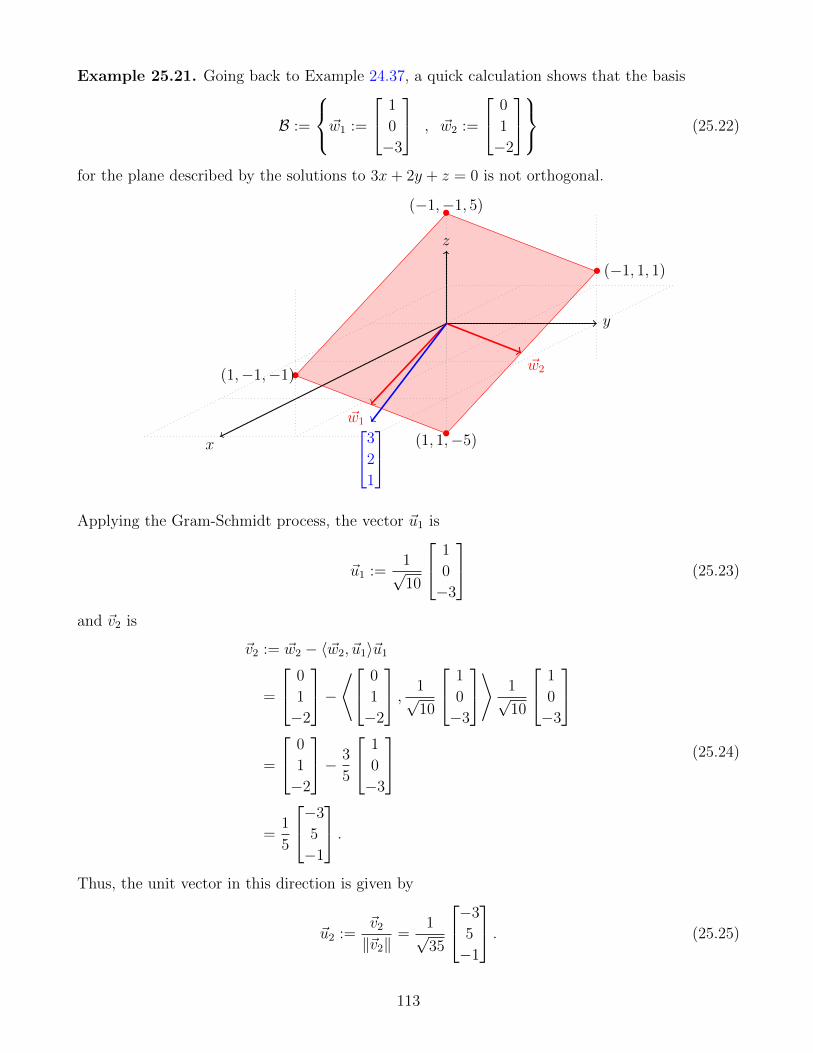
http://math.stackexchange.com/questions/1303977/what-is-the-idea-behind-a-projection-operator-what-does-it-do

http://math.stackexchange.com/questions/1303977/what-is-the-idea-behind-a-projection-operator-what-does-it-do

Example 25.21. Going back to Example 24.37, a quick calculation shows that the basis

B :=

~w1 :=

1

0

−3

, ~w2 :=

0

1

−2

(25.22)

for the plane described by the solutions to 3x+ 2y + z = 0 is not orthogonal.

x

y

z

•(−1,−1, 5)

• (−1, 1, 1)

•(1, 1,−5)

•(1,−1,−1)

~w1

~w2

3

2

1

Applying the Gram-Schmidt process, the vector ~u1 is

~u1 :=1√10

1

0

−3

(25.23)

and ~v2 is

~v2 := ~w2 − 〈~w2, ~u1〉~u1

=

0

1

−2

−⟨ 0

1

−2

, 1√10

1

0

−3

⟩ 1√10

1

0

−3

=

0

1

−2

− 3

5

1

0

−3

=

1

5

−3

5

−1

.

(25.24)

Thus, the unit vector in this direction is given by

~u2 :=~v2

‖~v2‖=

1√35

−3

5

−1

. (25.25)

113

x

y

z

~u1~u2

Now consider the vector

~v :=

1

2

−2

. (25.26)

The projection of this vector onto the plane W spanned by B is given by

PW (~v) = 〈~v, ~u1〉~u1 + 〈~v, ~u2〉~u2

=

⟨ 1

2

−2

, 1√10

1

0

−3

⟩ 1√10

1

0

−3

+

⟨ 1

2

−2

, 1√35

−3

5

−1

⟩ 1√35

−3

5

−1

=

7

10

1

0

−3

+18

35

−3

5

−1

=

1

35

−1

18

33

(25.27)

x

y

z

~v

PW (~v)

This construction allows us to quickly prove Theorem 25.1.

114

Proof of Theorem 25.1. Let S be an orthonormal set for W, the existence of which is guaranteed

by the Gram-Schmidt process. Then apply Theorem 25.7.

Homework (Due: Tuesday December 6). Please check HuskyCT for the homework. Please show


we covered parts of Sections 6.2, 6.3, and 6.4.

115

26 December 1

Quiz (review of what we covered on Nov 15 and Nov 17) at the beginning of class!

A few lectures ago, we asked what are sufficient conditions for a matrix to be diagonalizable.

Today, we will learn about such conditions as well as a useful decomposition for any matrix.

Definition 26.1. An m× n matrix A is symmetric whenever AT = A.

A similar definition can be made for complex matrices.

Definition 26.2. Let A be an m× n matrix with possibly complex entries

A =

a11 a12 · · · a1n

a21 a22 · · · a2n

......

. . ....

...


. (26.3)

The conjugate transpose of A is the n×m matrix

A† :=

a11 a21 · · · am1

a12 a22 · · · am2

......

. . ....

...

a1n a2n · · · amn

. (26.4)

The superscript † is pronounced “dagger.”

Definition 26.5. An m× n matrix A is Hermitian whenever A† = A.

Example 26.6. The three matrices

σx =

[0 1

1 0

], σy =

[0 −ii 0

], & σz =

[1 0

0 −1

](26.7)

are all Hermitian. Notice that the eigenvalues of these three matrices are all ±1, which are real.

We will say something about this phenomenon soon.

Exercise 26.8. Show that σx, σy, σz,12 is a basis for the real vector space of Hermitian 2 × 2

matrices (although we are using complex entries for some of the coordinates, we are only allowed

to multiply by real numbers—indeed, if we multiply a Hermitian matrix by a purely imaginary

number, the matrix will no longer be Hermitian).

Definition 26.9. An inner product on a complex vector space V is a function

〈 · , · 〉 : V × V → C (26.10)

satisfying analogous axioms as an inner product on a real vector space but with axiom (a) replaced

by

116

(a) For any two vectors ~v and ~u in V,

〈~v, ~u〉 = 〈~u,~v〉. (26.11)

This change of axiom implies that for any two vectors ~v and ~u in V and for any complex number

z ∈ C,〈z~u,~v〉 = 〈~v, z~u〉 = z〈~v, ~u〉 = z〈~v, ~u〉 = z〈~u,~v〉. (26.12)

Theorem 26.13. Let A be a complex m× n matrix. Then

〈~v, A~w〉 = 〈A†~v, ~w〉 (26.14)

for all vectors ~w in Cn and ~v in Cm.

Proof. A calculation easily proves this.

Theorem 26.15. The eigenvalues of a Hermitian matrix are real.

Proof. Let A be a Hermitian matrix and let λ be an eigenvalue with a corresponding eigenvector

~v. Then

λ〈~v,~v〉 = 〈~v, λ~v〉 = 〈~v, A~v〉 = 〈A†~v,~v〉 = 〈A~v,~v〉 = 〈λ~v,~v〉 = λ〈~v,~v〉 (26.16)

Since ~v is nonzero, 〈~v,~v〉 is nonzero as well, and this shows that λ = λ, i.e. λ is real.

Theorem 26.17. Let A be a Hermitian matrix. Then eigenvectors corresponding to different

eigenvalues are orthogonal. An analogous statement holds for symmetric real matrices provided

one considers real eigenvalues.

Proof. Let λ1 and λ2 be two distinct eigenvalues of A and let ~v1 and ~v2 be corresponding eigen-

vectors. Then

λ2〈~v1, ~v2〉 = 〈~v1, λ2~v2〉= 〈~v1, A~v2〉= 〈A†~v1, ~v2〉= 〈A~v1, ~v2〉= 〈λ1~v1, ~v2〉= λ1〈~v1, ~v2〉= λ1〈~v1, ~v2〉,

(26.18)

where in the last step we used the fact that eigenvalues of Hermitian matrices are real. This

calculation shows that

(λ2 − λ1)〈~v1, ~v2〉 = 0, (26.19)

which is only possible if either λ2−λ1 = 0 or 〈~v1, ~v2〉 = 0. However, by assumption, since λ1 6= λ2,

it follows that λ2 − λ1 6= 0. Hence 〈~v1, ~v2〉 = 0 which means that ~v1 is orthogonal to ~v2.

Theorem 26.20. A matrix A is Hermitian if and only if there exists a diagonal matrix D and a

matrix P all of whose columns are orthogonal such that A = PDP−1.

117

In fact, let A be an n× n Hermitian matrix, let

D :=

λ1 0 · · · 0

0 λ2...

.... . . 0

0 · · · 0 λn

(26.21)

be a diagonal matrix of its eigenvalues, and let

P :=

~u1 · · · ~un

(26.22)

be the matrix of orthonormal eigenvectors (given a matrix P that initially might have all orthogonal

eigenvectors, one can simply scale them so that they have unit length). Then, a quick calculation

shows that

P † = P−1. (26.23)

Using this, the previous theorem says that

A =

~u1 · · · ~un

λ1 0 · · · 0

0 λ2...

.... . . 0

0 · · · 0 λn

~u1 · · · ~un

† =n∑k=1

λk~uk~u†k. (26.24)

Notice that Pk := ~uk~u†k is an n×n matrix satisfying P 2

k = Pk. In fact, this operator is the projection

operator onto the subspace span~uk. Hence,

A =n∑k=1

λkPk (26.25)

provides a formula for the Hermitian matrix A as a weighted sum of projection operators onto

orthogonal one-dimensional subspaces of A generated by the eigenvectors of A. This decomposition

is referred to as the spectral decomposition of A.

Example 26.26. Consider the matrix

σy =

[0 −ii 0

](26.27)

from Example 26.6. The eigenvalues are λ↑y = +1 and λ↓y = −1 with corresponding eigenvectors

given by

~v↑y =

[1

i

]& ~v↓y =

[i

1

](26.28)

respectively. Associated normalized vectors are

~u↑y =1√2

[1

i

]. & ~u↓y =

1√2

[i

1

](26.29)

118

Then, the orthogonal matrix Py that diagonalizes σy is given by

Py =

[1/√

2 i/√

2

i/√

2 1/√

2

](26.30)

as we can check39

Py

[λ↑y 0

0 λ−y

]P †y =

1

2

[1 i

i 1

] [1 0

0 −1

] [1 −i−i 1

]=

[0 −ii 0

]= σy (26.31)

and the projection matrices P ↑y and P ↓y that project onto the eigenspaces span(~u↑y

)and span

(~u↓y

),

respectively, are given by (each calculated in two different ways to illustrate the possible methods)40

P ↑y = ~u↑y~u↑†y =

(1√2

[1

i

])(1√2

[1 −i

])=

[1/2 −i/2i/2 1/2

](26.32)

and41

P ↓y =

⟨~u↓y, ~e1

⟩~u↓y

⟨~u↓y, ~e2

⟩~u↓y

=1

2

⟨[

i

1

],

[1

0

]⟩[i

1

] ⟨[i

1

],

[0

1

]⟩[i

1

] =

[1/2 i/2

−i/2 1/2

].

(26.33)

Therefore, the matrix σy decomposes as

σy = λ↑yP↑y + λ↓yP

↓y = 1

[1/2 −i/2i/2 1/2

]− 1

[1/2 i/2

−i/2 1/2

]. (26.34)

The only reason this looks more complicated than the matrix σy is because the matrix is expressed

in the basis ~e1, ~e2. If we expressed this matrix in the basis Y := ~u↑y, ~u↓y it looks significantly

simpler

[σy]Y =

[1 0

0 −1

]Y. (26.35)

Example 26.36. For the record, consider the matrix σz from Example 26.6. The eigenvalues are

λ↑z = +1 and λ↓z = −1 with corresponding normalized eigenvectors given by

~u↑z =

[1

0

]& ~u↓z =

[0

1

](26.37)

39For a complex matrix P with orthogonal columns, the inverse P−1 is given by P † instead of PT , which is what

happens when P is real.40In Dirac bra-ket notation, this reads P ↑y = |~u↑y〉〈~u↑y|.41Remember, the matrix A associated to a linear transformation C2 T←− C2 is given by

A =

T (~e1) T (~e2)

.

119

respectively. The projection operators onto these eigenspaces are easy to read off because the

matrix σz is already in diagonal form. These projections are

P ↑z =

[1 0

0 0

]& P ↓z =

[0 0

0 1

]. (26.38)

Example 26.39 (The Stern-Gerlach experiment and quantum mechanics). Consider the following

experiment where (light) classical magnets are sent through a specific type of magnetic field (fixed

throughout the experiment). Depending on the orientation of the magnet, the deflection will be

distributed continuously according to this orientation. However, if a silver atom is sent through

the same apparatus, its deflection is more discrete. It is either only sent up or down. The silver

atoms are show out of an oven so that their internal properties are distributed as uniformly as

possible.

Watch video at: https://upload.wikimedia.org/wikipedia/commons/9/9e/Quantum_spin_

and_the_Stern-Gerlach_experiment.ogv

Let us visualize this Stern-Gerlach experiment by the following cartoon (read from right to

left).

AgovenSG

Z

50% ↑ along z

50% ↓ along z

Now, imagine a second experiment where we isolate the silver atoms that were deflected up along

the z axis and we send those atoms through a Stern-Gerlach experiment oriented along the y axis.

Experimentally, we find that on average 50% of the atoms are deflected in the positive y direction

and 50% in the negative y direction with the same magnitude as the deflection in the z direction

from the first experiment.

AgovenSG

Z

↑ along z

↓ along z

SGY

50% ↑ along y

50% ↓ along y

What do you think happens if we take the atoms that were deflected in the positive z direction first,

then deflected in the positive y direction, and we send these through yet another Stern-Gerlach

experiment oriented again back along the z direction?

AgovenSG

Z

↑ z

↓ zSGY

↑ y

↓ ySGZ

50% ↑ along z

50% ↓ along z

It turns out that not all of them will still deflect in the positive z direction. Instead, 50% of

these atoms will be deflected in the positive z direction and 50% in the negative z direction!

Preposterous! How can we possibly explain this phenomenon?

120

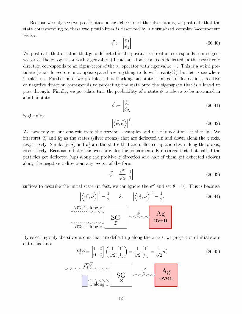
https://upload.wikimedia.org/wikipedia/commons/9/9e/Quantum_spin_and_the_Stern-Gerlach_experiment.ogv

https://upload.wikimedia.org/wikipedia/commons/9/9e/Quantum_spin_and_the_Stern-Gerlach_experiment.ogv

Because we only see two possibilities in the deflection of the silver atoms, we postulate that the

state corresponding to these two possibilities is described by a normalized complex 2-component

vector.

~ψ :=

[ψ1

ψ2

](26.40)

We postulate that an atom that gets deflected in the positive z direction corresponds to an eigen-

vector of the σz operator with eigenvalue +1 and an atom that gets deflected in the negative z

direction corresponds to an eigenvector of the σz operator with eigenvalue −1. This is a weird pos-

tulate (what do vectors in complex space have anything to do with reality!?), but let us see where

it takes us. Furthermore, we postulate that blocking out states that get deflected in a positive

or negative direction corresponds to projecting the state onto the eigenspace that is allowed to

pass through. Finally, we postulate that the probability of a state ~ψ as above to be measured in

another state

~φ :=

[φ1

φ2

](26.41)

is given by ∣∣∣⟨~φ, ~ψ⟩∣∣∣2 . (26.42)

We now rely on our analysis from the previous examples and use the notation set therein. We

interpret ~u↑z and ~u↓z as the states (silver atoms) that are deflected up and down along the z axis,

respectively. Similarly, ~u↑y and ~u↓y are the states that are deflected up and down along the y axis,

respectively. Because initially the oven provides the experimentally observed fact that half of the

particles get deflected (up) along the positive z direction and half of them get deflected (down)

along the negative z direction, any vector of the form

~ψ =eiθ√

2

[1

1

](26.43)

suffices to describe the initial state (in fact, we can ignore the eiθ and set θ = 0). This is because∣∣∣⟨~u↑z, ~ψ⟩∣∣∣2 =1

2&

∣∣∣⟨~u↓z, ~ψ⟩∣∣∣2 =1

2. (26.44)

Agoven

~ψSGZ

50% ↑ along z

50% ↓ along z

By selecting only the silver atoms that are deflect up along the z axis, we project our initial state

onto this state

P ↑z~ψ =

[1 0

0 0

](1√2

[1

1

])=

1√2

[1

0

]=

1√2~u↑z (26.45)

Agoven

~ψSGZ

P ↑z~ψ

↓ along z

121

and then we normalize this state to ~u↑z so that our probabilistic interpretation will still hold. In

the second experiment, this state gets sent through the Stern-Gerlach apparatus oriented along

the y direction. Let us check that indeed half of the particles are deflected up along the y direction

and the other half are deflected down.∣∣⟨~u↑y, ~u↑z⟩∣∣2 =1

2&

∣∣⟨~u↓y, ~u↑z⟩∣∣2 =1

2. (26.46)

Agoven

~ψSGZ

P ↑z~ψ

↓ along z

SGY

50% ↑ along y

50% ↓ along y

So far so good. Now let’s put these postulates to the ultimate test of projecting our resulting state

onto the up state along the y direction to obtain

P ↑y ~u↑z =

1√2~u↑y (26.47)

Agoven

~ψSGZ

P ↑z~ψ

↓ zSGY

P ↑yP↑z~ψ

↓ y

and again normalize to obtain just ~u↑y. Now let’s send these silver atoms back to another Stern-

Gerlach apparatus oriented along the z direction. So what does the math tell us? The probabilities

of this resulting state deflecting either up or down along the z axis after going through all these

experiments is ∣∣⟨~u↑z, ~u↑y⟩∣∣2 =1

2&

∣∣⟨~u↓z, ~u↑y⟩∣∣2 =1

2(26.48)

Agoven

~ψSGZ

P ↑z~ψ

↓ zSGY

P ↑yP↑z~ψ

↓ ySGZ

50% ↑ along z

50% ↓ along z

which beautifully agrees with the experiment! Is all of this a coincidence? We think not. And

it turns out that the study of abstract vector spaces is intimately related to other phenomena

centered around the subject called quantum mechanics. The effect described in this example is

due to the spin of an electron (in the case of silver, this is due to the single valence electron), a

feature inherent of particles and described adequately in the theory of quantum mechanics.

Homework (Due: Tuesday December 6). Please check HuskyCT for the homework. Please show


we covered Section 7.1 in Lay and additional material not in Lay.

122

27 December 6


Homework. Do the exam review and bring it to class on Thursday December 8. In this lecture,

we covered Section 7.4 in Lay.

123

28 December 8

There is no quiz. Today we will review for the final. Please look on HuksyCT for some sample

problems. Review quizzes, homework, suggested exercises, and class notes. Bring questions to

class.

124

References

[1] G. Polya, How to solve it: A new aspect of mathematical method, Princeton University Press, 2014.

125

math 2210q applied linear algebra, fall 2016parzygnat/math2210f16/notes/2210qfall2016no… · math...

Documents