math 167: applied linear algebra chapter 2 · math 167: applied linear algebra chapter 2 jesus de...

MATH 167: APPLIED LINEAR ALGEBRAChapter 2

Jesus De Loera, UC Davis

February 1, 2012

Jesus De Loera, UC Davis MATH 167: APPLIED LINEAR ALGEBRA Chapter 2

General LinearSystems of Equations (2.2).


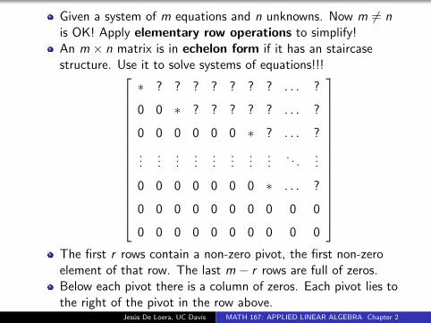
Given a system of m equations and n unknowns. Now m 6= nis OK! Apply elementary row operations to simplify!An m × n matrix is in echelon form if it has an staircasestructure. Use it to solve systems of equations!!!

∗ ? ? ? ? ? ? ? . . . ?

0 0 ∗ ? ? ? ? ? . . . ?

0 0 0 0 0 0 ∗ ? . . . ?

......

......

......

......

. . ....

0 0 0 0 0 0 0 ∗ . . . ?

0 0 0 0 0 0 0 0 0 0

0 0 0 0 0 0 0 0 0 0

The first r rows contain a non-zero pivot, the first non-zeroelement of that row. The last m − r rows are full of zeros.Below each pivot there is a column of zeros. Each pivot lies tothe right of the pivot in the row above.


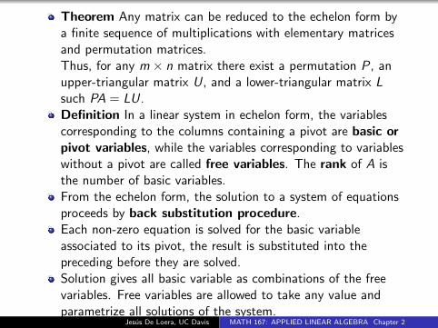
Theorem Any matrix can be reduced to the echelon form bya finite sequence of multiplications with elementary matricesand permutation matrices.Thus, for any m × n matrix there exist a permutation P, anupper-triangular matrix U, and a lower-triangular matrix Lsuch PA = LU.Definition In a linear system in echelon form, the variablescorresponding to the columns containing a pivot are basic orpivot variables, while the variables corresponding to variableswithout a pivot are called free variables. The rank of A isthe number of basic variables.From the echelon form, the solution to a system of equationsproceeds by back substitution procedure.Each non-zero equation is solved for the basic variableassociated to its pivot, the result is substituted into thepreceding before they are solved.Solution gives all basic variable as combinations of the freevariables. Free variables are allowed to take any value andparametrize all solutions of the system.


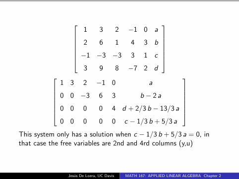
1 3 2 −1 0 a

2 6 1 4 3 b

−1 −3 −3 3 1 c

3 9 8 −7 2 d

1 3 2 −1 0 a

0 0 −3 6 3 b − 2 a

0 0 0 0 4 d + 2/3 b − 13/3 a

0 0 0 0 0 c − 1/3 b + 5/3 a

This system only has a solution when c − 1/3 b + 5/3 a = 0, inthat case the free variables are 2nd and 4rd columns (y,u)


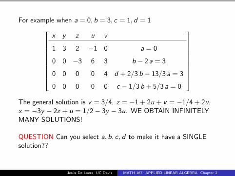
For example when a = 0, b = 3, c = 1, d = 1

x y z u v

1 3 2 −1 0 a = 0

0 0 −3 6 3 b − 2 a = 3

0 0 0 0 4 d + 2/3 b − 13/3 a = 3

0 0 0 0 0 c − 1/3 b + 5/3 a = 0

The general solution is v = 3/4, z = −1 + 2u + v = −1/4 + 2u,x = −3y − 2z + u = 1/2− 3y − 3u. WE OBTAIN INFINITELYMANY SOLUTIONS!

QUESTION Can you select a, b, c , d to make it have a SINGLEsolution??


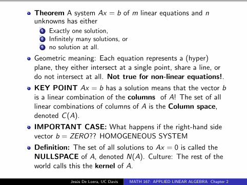
Theorem A system Ax = b of m linear equations and nunknowns has either

1 Exactly one solution,2 Infinitely many solutions, or3 no solution at all.

Geometric meaning: Each equation represents a (hyper)plane, they either intersect at a single point, share a line, ordo not intersect at all. Not true for non-linear equations!.

KEY POINT Ax = b has a solution means that the vector bis a linear combination of the columns of A! The set of alllinear combinations of columns of A is the Column space,denoted C (A).

IMPORTANT CASE: What happens if the right-hand sidevector b = ZERO?? HOMOGENEOUS SYSTEM

Definition: The set of all solutions to Ax = 0 is called theNULLSPACE of A, denoted N(A). Culture: The rest of theworld calls this the kernel of A.


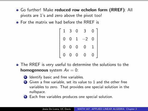
Go further! Make reduced row echelon form (RREF): Allpivots are 1’s and zero above the pivot too!

For the matrix we had before the RREF is1 3 0 3 0

0 0 1 −2 0

0 0 0 0 1

0 0 0 0 0

The RREF is very useful to determine the solutions to thehomogeneous system Ax = 0:

1 Identify basic and free variables.2 Given a free variable, set its value to 1 and the other free

variables to zero. That provides one special solution in thenullspace.

3 Each free variables produces one special solution.


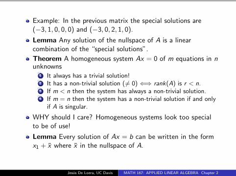
Example: In the previous matrix the special solutions are(−3, 1, 0, 0, 0) and (−3, 0, 2, 1, 0).

Lemma Any solution of the nullspace of A is a linearcombination of the “special solutions”.

Theorem A homogeneous system Ax = 0 of m equations in nunknowns

1 It always has a trivial solution!2 It has a non-trivial solution ( 6= 0) ⇐⇒ rank(A) is r < n.3 If m < n then the system has always a non-trivial solution.4 If m = n then the system has a non-trivial solution if and only

if A is singular.

WHY should I care? Homogeneous systems look too specialto be of use!

Lemma Every solution of Ax = b can be written in the formx1 + x where x in the nullspace of A.


Vector Spacesand Subspaces (2.1)


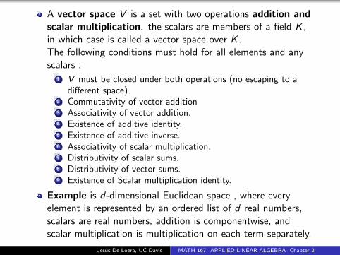
A vector space V is a set with two operations addition andscalar multiplication. the scalars are members of a field K ,in which case is called a vector space over K .The following conditions must hold for all elements and anyscalars :

1 V must be closed under both operations (no escaping to adifferent space).

2 Commutativity of vector addition3 Associativity of vector addition.4 Existence of additive identity.5 Existence of additive inverse.6 Associativity of scalar multiplication.7 Distributivity of scalar sums.8 Distributivity of vector sums.9 Existence of Scalar multiplication identity.

Example is d-dimensional Euclidean space , where everyelement is represented by an ordered list of d real numbers,scalars are real numbers, addition is componentwise, andscalar multiplication is multiplication on each term separately.


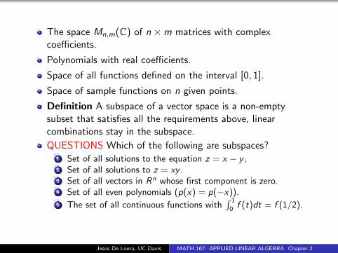
The space Mn,m(C) of n ×m matrices with complexcoefficients.

Polynomials with real coefficients.

Space of all functions defined on the interval [0, 1].

Space of sample functions on n given points.

Definition A subspace of a vector space is a non-emptysubset that satisfies all the requirements above, linearcombinations stay in the subspace.

QUESTIONS Which of the following are subspaces?1 Set of all solutions to the equation z = x − y ,2 Set of all solutions to z = xy .3 Set of all vectors in Rn whose first component is zero.4 Set of all even polynomials (p(x) = p(−x)).5 The set of all continuous functions with

∫ 1

0f (t)dt = f (1/2).


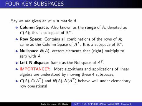
FOUR KEY SUBSPACES

Say we are given an m × n matrix A

Column Space: Also known as the range of A, denoted asC (A); this is subspace of Rm.

Row Space: Contains all combinations of the rows of A;same as the Column Space of AT . It is a subspace of Rn.

Nullspace N(A), vectors elements that (right) multiply tozero with A

Left Nullspace: Same as the Nullspace of AT .

IMPORTANCE?: Most algorithms and applications of linearalgebra are understood by moving these 4 subspaces.

C (A),C (AT ) and N(A),N(AT ) behave well under elementaryrow operations!


What are these 4 subspaces? (continued)

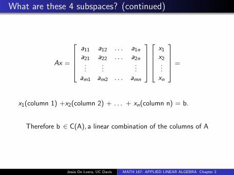
Ax =

a11 a12 . . . a1n

a21 a22 . . . a2n...

......

am1 am2 . . . amn

x1

x2...xn

=

x1(column 1) +x2(column 2) + . . . + xn(column n) = b.

Therefore b ∈ C(A), a linear combination of the columns of A


What are these 4 subspaces? (continued)

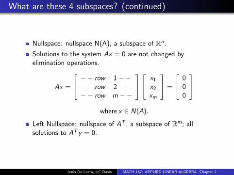
Nullspace: nullspace N(A), a subspace of Rn.

Solutions to the system Ax = 0 are not changed byelimination operations.

Ax =

−− row 1−−−− row 2−−−− row m −−

x1

x2

xm

=

000

where x ∈ N(A).

Left Nullspace: nullspace of AT , a subspace of Rm; allsolutions to AT y = 0.


Linear Independence,Basis, and Dimension (2.3)


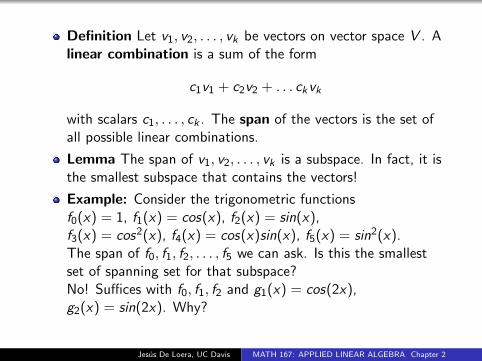
Definition Let v1, v2, . . . , vk be vectors on vector space V . Alinear combination is a sum of the form

c1v1 + c2v2 + . . . ckvk

with scalars c1, . . . , ck . The span of the vectors is the set ofall possible linear combinations.

Lemma The span of v1, v2, . . . , vk is a subspace. In fact, it isthe smallest subspace that contains the vectors!

Example: Consider the trigonometric functionsf0(x) = 1, f1(x) = cos(x), f2(x) = sin(x),f3(x) = cos2(x), f4(x) = cos(x)sin(x), f5(x) = sin2(x).The span of f0, f1, f2, . . . , f5 we can ask. Is this the smallestset of spanning set for that subspace?No! Suffices with f0, f1, f2 and g1(x) = cos(2x),g2(x) = sin(2x). Why?


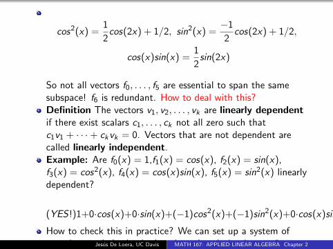
cos2(x) =1

2cos(2x) + 1/2, sin2(x) =

−1

2cos(2x) + 1/2,

cos(x)sin(x) =1

2sin(2x)

So not all vectors f0, . . . , f5 are essential to span the samesubspace! f6 is redundant. How to deal with this?Definition The vectors v1, v2, . . . , vk are linearly dependentif there exist scalars c1, . . . , ck not all zero such thatc1v1 + · · ·+ ckvk = 0. Vectors that are not dependent arecalled linearly independent.Example: Are f0(x) = 1,f1(x) = cos(x), f2(x) = sin(x),f3(x) = cos2(x), f4(x) = cos(x)sin(x), f5(x) = sin2(x) linearlydependent?

(YES!)1+0·cos(x)+0·sin(x)+(−1)cos2(x)+(−1)sin2(x)+0·cos(x)sin(x) = 0.

How to check this in practice? We can set up a system ofequations and check whether the only solution is ci = 0.Jesus De Loera, UC Davis MATH 167: APPLIED LINEAR ALGEBRA Chapter 2

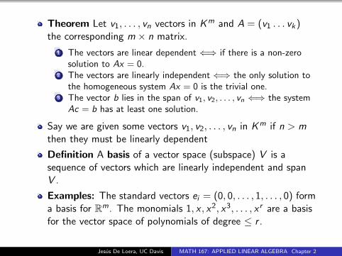
Theorem Let v1, . . . , vn vectors in Km and A = (v1 . . . vk)the corresponding m × n matrix.

1 The vectors are linear dependent ⇐⇒ if there is a non-zerosolution to Ax = 0.

2 The vectors are linearly independent ⇐⇒ the only solution tothe homogeneous system Ax = 0 is the trivial one.

3 The vector b lies in the span of v1, v2, . . . , vn ⇐⇒ the systemAc = b has at least one solution.

Say we are given some vectors v1, v2, . . . , vn in Km if n > mthen they must be linearly dependent

Definition A basis of a vector space (subspace) V is asequence of vectors which are linearly independent and spanV .

Examples: The standard vectors ei = (0, 0, . . . , 1, . . . , 0) forma basis for Rm. The monomials 1, x , x2, x3, . . . , x r are a basisfor the vector space of polynomials of degree ≤ r .


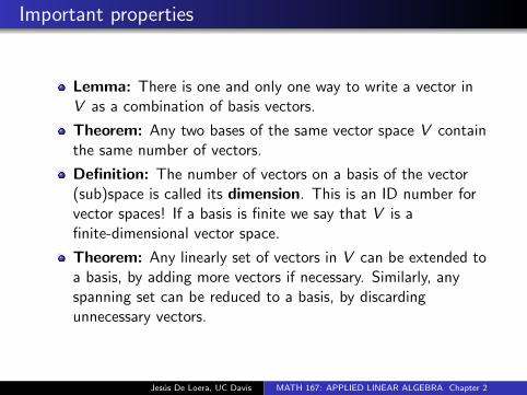
Important properties

Lemma: There is one and only one way to write a vector inV as a combination of basis vectors.

Theorem: Any two bases of the same vector space V containthe same number of vectors.

Definition: The number of vectors on a basis of the vector(sub)space is called its dimension. This is an ID number forvector spaces! If a basis is finite we say that V is afinite-dimensional vector space.

Theorem: Any linearly set of vectors in V can be extended toa basis, by adding more vectors if necessary. Similarly, anyspanning set can be reduced to a basis, by discardingunnecessary vectors.


The Four FundamentalSubspaces (2.4)


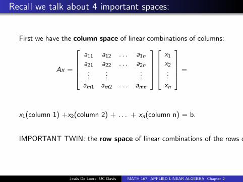
Recall we talk about 4 important spaces:

First we have the column space of linear combinations of columns:

Ax =

a11 a12 . . . a1n

a21 a22 . . . a2n...

......

am1 am2 . . . amn

x1

x2...xn

=

x1(column 1) +x2(column 2) + . . . + xn(column n) = b.

IMPORTANT TWIN: the row space of linear combinations of the rows of A


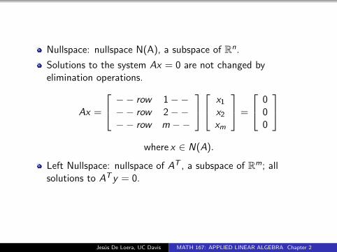
Nullspace: nullspace N(A), a subspace of Rn.

Solutions to the system Ax = 0 are not changed byelimination operations.

Ax =

−− row 1−−−− row 2−−−− row m −−

x1

x2

xm

=

000

where x ∈ N(A).

Left Nullspace: nullspace of AT , a subspace of Rm; allsolutions to AT y = 0.


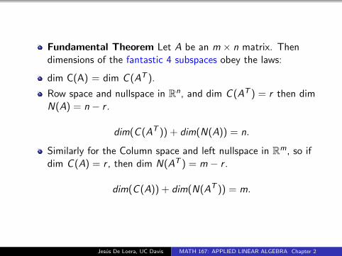
Fundamental Theorem Let A be an m × n matrix. Thendimensions of the fantastic 4 subspaces obey the laws:

dim C(A) = dim C (AT ).

Row space and nullspace in Rn, and dim C (AT ) = r then dimN(A) = n − r .

dim(C (AT )) + dim(N(A)) = n.

Similarly for the Column space and left nullspace in Rm, so ifdim C (A) = r , then dim N(AT ) = m − r .

dim(C (A)) + dim(N(AT )) = m.


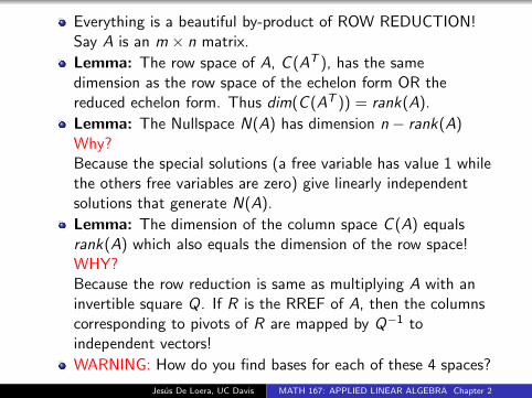
Everything is a beautiful by-product of ROW REDUCTION!Say A is an m × n matrix.

Lemma: The row space of A, C (AT ), has the samedimension as the row space of the echelon form OR thereduced echelon form. Thus dim(C (AT )) = rank(A).

Lemma: The Nullspace N(A) has dimension n − rank(A)Why?Because the special solutions (a free variable has value 1 whilethe others free variables are zero) give linearly independentsolutions that generate N(A).

Lemma: The dimension of the column space C (A) equalsrank(A) which also equals the dimension of the row space!WHY?Because the row reduction is same as multiplying A with aninvertible square Q. If R is the RREF of A, then the columnscorresponding to pivots of R are mapped by Q−1 toindependent vectors!

WARNING: How do you find bases for each of these 4 spaces?


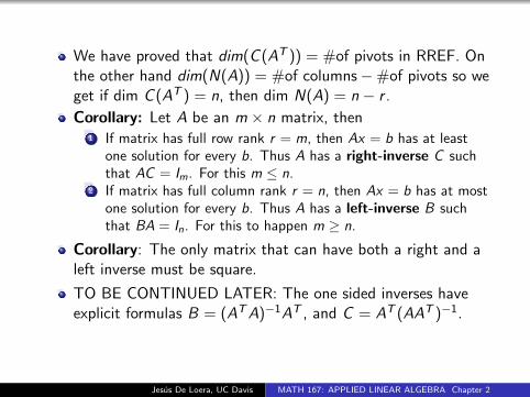
We have proved that dim(C (AT )) = #of pivots in RREF. Onthe other hand dim(N(A)) = #of columns−#of pivots so weget if dim C (AT ) = n, then dim N(A) = n − r .

Corollary: Let A be an m × n matrix, then1 If matrix has full row rank r = m, then Ax = b has at least

one solution for every b. Thus A has a right-inverse C suchthat AC = Im. For this m ≤ n.

2 If matrix has full column rank r = n, then Ax = b has at mostone solution for every b. Thus A has a left-inverse B suchthat BA = In. For this to happen m ≥ n.

Corollary: The only matrix that can have both a right and aleft inverse must be square.

TO BE CONTINUED LATER: The one sided inverses haveexplicit formulas B = (ATA)−1AT , and C = AT (AAT )−1.


Linear Transformations (2.6)


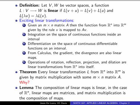
Definition: Let V ,W be vector spaces, a functionL : V −→W is linear if L(v + u) = L(v) + L(u) andL(λv) = λL(v).Exciting linear transformations:

1 Given an m × n matrix A then the function from Rn into Rm

given by the rule v is mapped to Av .2 Integration on the space of continuous functions inside an

interval3 Differentiation on the space of continuous differentiable

functions on an interval.4 From Calculus, the gradient, the divergence are also linear

maps.5 Operations of rotation, reflection, projection, and dilation are

linear transformations from Rn into itself.

Theorem Every linear transformation L from Rn into Rm isgiven by matrix multiplication with some m × n matrix A.Why?Lemma The composition of linear maps is linear, in the caseof Rn, linear maps are matrices, and matrix multiplication isthe composition of maps.


math 167: applied linear algebra chapter 2 · math 167: applied linear algebra chapter 2 jesus de...

Documents