Manual for LS-DYNASoil Material Model 147

PUBLICATION NO. FHWA-HRT-04-095 NOVEMBER 2004

Research, Development, and TechnologyTurner-Fairbank Highway Research Center6300 Georgetown PikeMcLean, VA 22101-2296

Manual for LS-DYNA Soil Material Model 147 FHWA-HRT-04-095

November 2004 Federal Highway Administration Research and Development Turner-Fairbank Highway Research Center 6300 Georgetown Pike McLean, VA 22101-2296

Foreword This report documents a soil material model that has been implemented into the dynamic finite element code, LS-DYNA, beginning with version 970. This material model was developed specifically to predict the dynamic performance of the foundation soil in which roadside safety structures are mounted when undergoing a collision by a motor vehicle. This model is applicable for all soil types when one surface is exposed to the elements if the appropriate material coefficients are inserted. Default material coefficients for National Cooperative Highway Research Program (NCHRP) Report 350, Strong Soil, are stored in the model and can be accessed for use. This report is one of two that completely documents this material model. This report, Manual for LS-DYNA Soil Material Model 147 (FHWA-HRT-04-095), completely documents this material model for the user. The second report, Evaluation of LS-DYNA Soil Material Model 147 (FHWA-HRT-04-094), completely documents the model’s performance and the accuracy of the results. This performance evaluation was a collaboration between the model developer and the model evaluator. Regarding the model performance evaluation, the developer and evaluator were unable to come to a final agreement regarding the model’s performance and accuracy. (The material coefficients for the default soil result in a soil foundation that may be stiffer than desired.) These disagreements are listed and thoroughly discussed in section 9 of the second report. This report will be of interest to research engineers associated with the evaluation and crashworthy performance of roadside safety structures, particularly those engineers responsible for the prediction of the crash response of such structures when using the finite element code LS-DYNA.

Michael F. Trentacoste Director, Office of Safety Research and Development

Notice This document is disseminated under the sponsorship of the U.S. Department of Transportation in the interest of information exchange. The U.S. Government assumes no liability for the use of the information contained in this document. This report does not constitute a standard, specification, or regulation. The U.S. Government does not endorse products or manufacturers. Trademarks or manufacturers' names appear in this report only because they are considered essential to the objective of the document.

Quality Assurance Statement The Federal Highway Administration (FHWA) provides high-quality information to serve Government, industry, and the public in a manner that promotes public understanding. Standards and policies are used to ensure and maximize the quality, objectivity, utility, and integrity of its information. FHWA periodically reviews quality issues and adjusts its programs and processes to ensure continuous quality improvement.

Technical Report Documentation Page 1. Report No.

FHWA-HRT-04-095 2. Government Accession No.

3. Recipient’s Catalog No.

5. Report Date November 2004

4. Title and Subtitle

MANUAL FOR LS-DYNA SOIL MATERIAL MODEL 147 6. Performing Organization Code

7. Author(s)

Brett A. Lewis, Ph.D. 8. Performing Organization Report No.

9. Performing Organization Name and Address

APTEK, Inc. 1257 Lake Plaza Drive Colorado Springs, CO 80906

10. Work Unit No. (TRAIS)

11. Contract or Grant No.

DTFH61-98-C-00071 13. Type of Report and Period Covered

Final Report 09-28-1998 through 08-31-2004

12. Sponsoring Agency’s Name and Address Volpe National Transportation Systems Center 55 Broadway, Kendall Square Cambridge, MA 02142-1093 Federal Highway Administration 6300 Georgetown Pike McLean, VA 22101-2296

14. Sponsoring Agency’s Code

15. Supplementary Notes

Contracting Officer’s Technical Representative (COTR): Martin Hargrave, Office of Safety Research and Development, HRDS-04, Turner-Fairbank Highway Research Center

16. Abstract

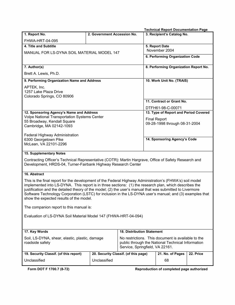
This is the final report for the development of the Federal Highway Administration’s (FHWA’s) soil model implemented into LS-DYNA. This report is in three sections: (1) the research plan, which describes the justification and the detailed theory of the model; (2) the user’s manual that was submitted to Livermore Software Technology Corporation (LSTC) for inclusion in the LS-DYNA user’s manual; and (3) examples that show the expected results of the model. The companion report to this manual is: Evaluation of LS-DYNA Soil Material Model 147 (FHWA-HRT-04-094)

17. Key Words

Soil, LS-DYNA, shear, elastic, plastic, damage roadside safety

18. Distribution Statement

No restrictions. This document is available to the public through the National Technical Information Service, Springfield, VA 22161.

19. Security Classif. (of this report)

Unclassified

20. Security Classif. (of this page)

Unclassified

21. No. of Pages

68

22. Price

Form DOT F 1700.7 (8-72) Reproduction of completed page authorized

ii

Preface

The goal of the work performed under this program, Development of DYNA3D Analysis Tools for Roadside Safety Applications, is to develop soil and wood material models, implement the models into the LS-DYNA finite element code, and evaluate the performance of each model through correlations with available test data.(1) This work was performed under Federal Highway Administration (FHWA) Contract No. DTFH61-98-C-00071. The FHWA Contracting Officer’s Technical Representative (COTR) was Martin Hargrave. Two reports are available for each material model. One report is a user’s manual, Manual for LS-DYNA Soil Material Model 147; the second report is a performance evaluation, Evaluation of LS-DYNA Soil Material Model 147.(2) The user’s manual thoroughly documents the soil model theory, reviews the model input, and provides example problems for use as a learning tool. The performance evaluation for the soil model documents LS-DYNA parametric studies and correlations with test data performed by a potential end user of the soil model, along with commentary from the developer. The reader is urged to review this user’s manual before reading the evaluation report. A user’s manual(3) and evaluation report(4) are also available for the wood model. The model developer and evaluator were unable to come to a final agreement regarding several issues associated with the model’s performance and accuracy during the second independent evaluation of the soil model. These issues are listed and thoroughly discussed in section 9 of the soil model evaluation report.(2)

iii

SI* (MODERN METRIC) CONVERSION FACTORS APPROXIMATE CONVERSIONS TO SI UNITS

Symbol When You Know Multiply By To Find Symbol LENGTH

in inches 25.4 millimeters mm ft feet 0.305 meters m yd yards 0.914 meters m mi miles 1.61 kilometers km

AREA in2 square inches 645.2 square millimeters mm2

ft2 square feet 0.093 square meters m2

yd2 square yard 0.836 square meters m2

ac acres 0.405 hectares ha mi2 square miles 2.59 square kilometers km2

VOLUME fl oz fluid ounces 29.57 milliliters mL gal gallons 3.785 liters L ft3 cubic feet 0.028 cubic meters m3

yd3 cubic yards 0.765 cubic meters m3

NOTE: volumes greater than 1000 L shall be shown in m3

MASS oz ounces 28.35 grams glb pounds 0.454 kilograms kgT short tons (2000 lb) 0.907 megagrams (or "metric ton") Mg (or "t")

TEMPERATURE (exact degrees) oF Fahrenheit 5 (F-32)/9 Celsius oC

or (F-32)/1.8 ILLUMINATION

fc foot-candles 10.76 lux lx fl foot-Lamberts 3.426 candela/m2 cd/m2

FORCE and PRESSURE or STRESS lbf poundforce 4.45 newtons N lbf/in2 poundforce per square inch 6.89 kilopascals kPa

APPROXIMATE CONVERSIONS FROM SI UNITS Symbol When You Know Multiply By To Find Symbol

LENGTHmm millimeters 0.039 inches in m meters 3.28 feet ft m meters 1.09 yards yd km kilometers 0.621 miles mi

AREA mm2 square millimeters 0.0016 square inches in2

m2 square meters 10.764 square feet ft2

m2 square meters 1.195 square yards yd2

ha hectares 2.47 acres ac km2 square kilometers 0.386 square miles mi2

VOLUME mL milliliters 0.034 fluid ounces fl oz L liters 0.264 gallons gal m3 cubic meters 35.314 cubic feet ft3

m3 cubic meters 1.307 cubic yards yd3

MASS g grams 0.035 ounces ozkg kilograms 2.202 pounds lbMg (or "t") megagrams (or "metric ton") 1.103 short tons (2000 lb) T

TEMPERATURE (exact degrees) oC Celsius 1.8C+32 Fahrenheit oF

ILLUMINATION lx lux 0.0929 foot-candles fc cd/m2 candela/m2 0.2919 foot-Lamberts fl

FORCE and PRESSURE or STRESS N newtons 0.225 poundforce lbf kPa kilopascals 0.145 poundforce per square inch lbf/in2

*SI is the symbol for th International System of Units. Appropriate rounding should be made to comply with Section 4 of ASTM E380. e(Revised March 2003)

iv

Table of Contents

CHAPTER 1. THEORY MANUAL .............................................................. 1

INTRODUCTION..................................................................................................... 1

PRELIMINARY WORK ........................................................................................... 2

Determination of Critical Behaviors ................................................................. 2

Evaluation of the Utility of Models Already in LS-DYNA.................................. 7

MODEL DEVELOPMENT....................................................................................... 9

Elastic Constitutive Behavior........................................................................... 9

Yield Surface Behavior.................................................................................. 10

Excess Pore-Water Pressure Behavior ......................................................... 13

Strain Hardening Behavior ............................................................................ 16

Strain Softening Behavior.............................................................................. 18

Strain-Rate Behavior ..................................................................................... 21

INCORPORATION INTO LS-DYNA ..................................................................... 22

CHAPTER 2. USER’S MANUAL............................................................... 27

USER INPUT GUIDE ............................................................................................ 29

THEORY MANUAL............................................................................................... 31

DISCUSSION OF SOIL MODEL USE .................................................................. 39

CHAPTER 3. EXAMPLES MANUAL ....................................................... 41

CHAPTER 4. SUMMARY .......................................................................... 49

APPENDIX A. DETERMINATION OF PLASTICITY GRADIENTS .......... 51

v

APPENDIX B. EXAMPLES OF INPUT.................................................... 55

INPUT FOR SINGLE-ELEMENT SIMULATION OF 3.4-MPA TRIAXIAL COMPRESSION TEST ......................................................................................... 55

FHWA MATERIAL MODEL INPUT FOR DIRECT SHEAR EXAMPLE................ 58

REFERENCES........................................................................................... 59

vi

List of Figures

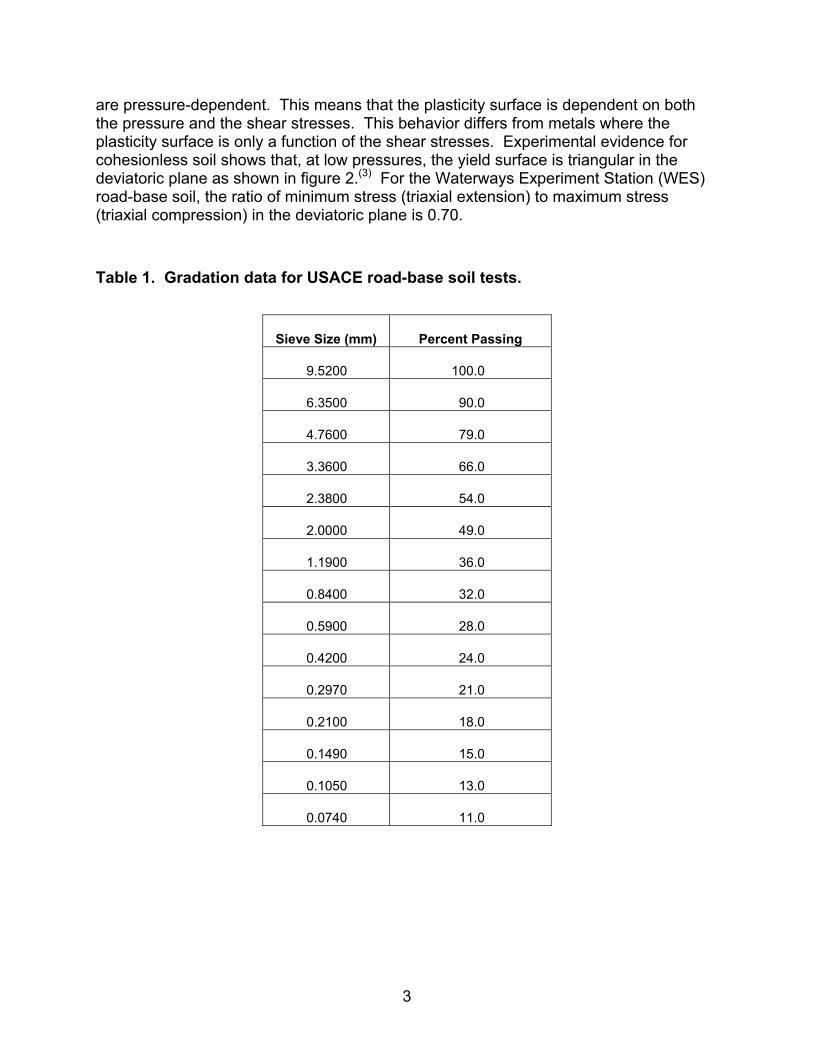
Figure 1. (a) Pressure-dependent (Mohr-Coulomb) and (b) pressure-independent (Von

Mises) yield surfaces....................................................................................... 4

Figure 2. Yield surface in deviatoric plane for cohesionless soils................................... 4

Figure 3. Principal stress difference (peak shear strength) versus pressure (average normal stress) for road-base material ............................................................. 5

Figure 4. Force deflection for two steel posts in soil tests with different moisture contents (5 percent and 26 percent) ............................................................... 6

Figure 5. Energy versus deflection for two steel posts in soil bogie tests with different moisture contents............................................................................................ 7

Figure 6. Model 25 single-element run, triaxial compression at 3.4 MPa compared to WES data..................................................................................................... 8

Figure 7. Pressure versus volumetric strain showing the effects of the D1 parameter.. 10

Figure 8. Standard Mohr-Coulomb yield surface in principal stress space................... 12

Figure 9. Comparison of Mohr-Coulomb yield surfaces in shear stress―Pressure space (standard—(A)/green, modified—(B)/red)........................................... 12

Figure 10. Yield surface with e = 0.55. ......................................................................... 13

Figure 11. Effects on pressure because of pore-water pressure.................................. 14

Figure 12. Effects of parameters on pore-water pressure. ........................................... 16

Figure 13. Principal stress difference versus principal strain difference for triaxial compression test at σ2 = 6.9 MPa of WES road-base material .................. 17

Figure 14. Hardening of yield surface........................................................................... 17

Figure 15. Principal stress difference versus axial strain for triaxial compression test at σ2 = 6.9 MPa of WES road-base material .................................................. 18

Figure 16. Definition of the void formation parameter. ................................................. 20

Figure 17. Zeta versus strain rate for different parameters. ......................................... 21 Figure 18. Elastic moduli and undamaged stresses. .................................................... 22

vii

Figure 19. Elastic trial stresses .................................................................................... 22 Figure 20. Determination of plastic strains ................................................................... 23 Figure 21. Update of stresses and history variables .................................................... 24 Figure 22. Viscoplasticity update.................................................................................. 24 Figure 23. Damage update........................................................................................... 25

Figure 24. Pressure versus volumetric strain showing the effects of the D1 parameter 34

Figure 25. Effects on pressure caused by pore-water pressure. .................................. 35

Figure 26. Effects of D2 and Ksk parameters on pore-water pressure........................... 37

Figure 27. Z-stress versus time for single-element 3.4-MPa triaxial compression simulation ................................................................................................... 41

Figure 28. LS-DYNA model of direct shear test DS-4. ................................................. 42

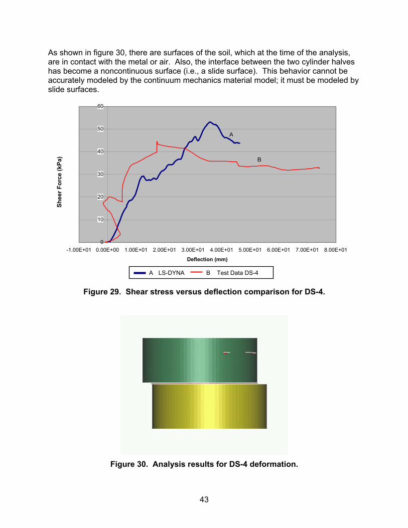
Figure 29. Shear stress versus deflection comparison for DS-4. ................................. 43

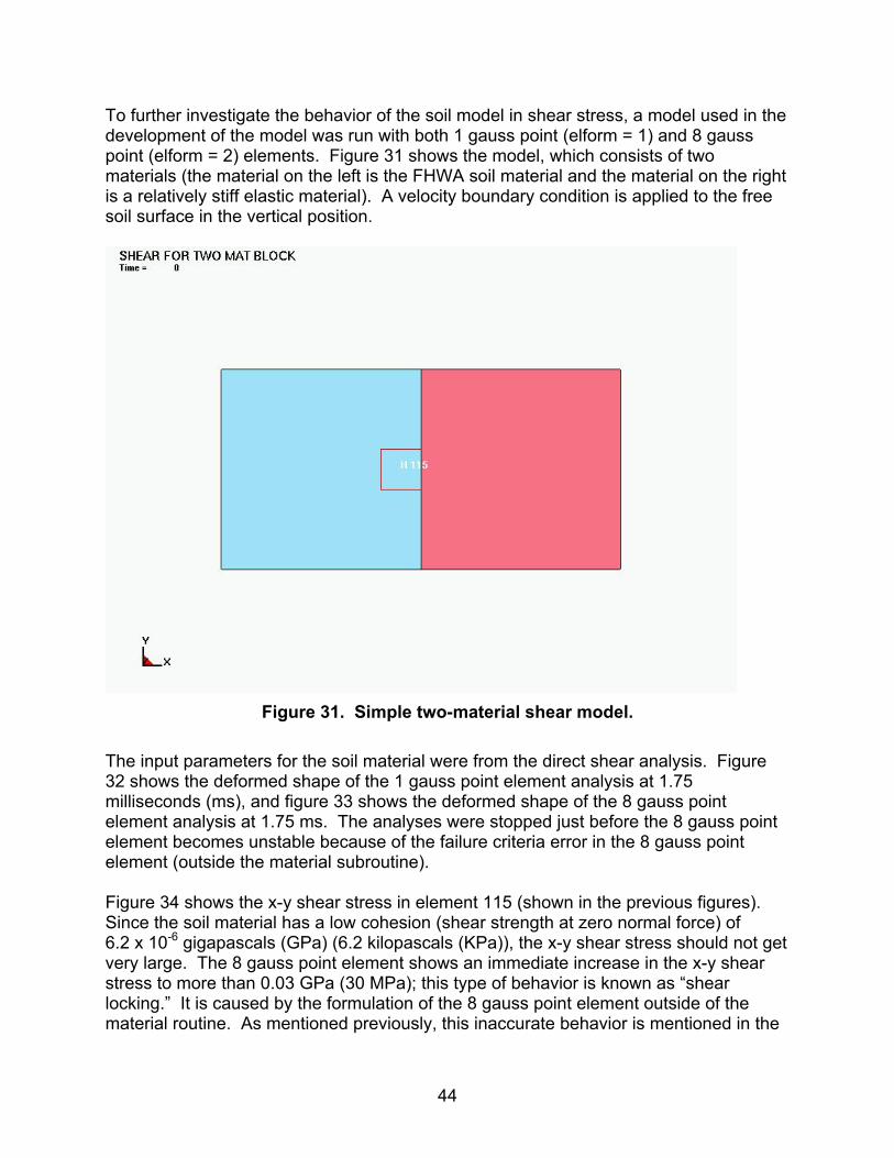
Figure 30. Analysis results for DS-4 deformation. ........................................................ 43

Figure 31. Simple two-material shear model. ............................................................... 44

Figure 32. Deformed shape of 1 gauss point element analysis.................................... 45

Figure 33. Deformed shape of 8 gauss point element analysis.................................... 46

Figure 34. Comparison of x-y stress at element 115 for 1 gauss point and 8 gauss point elements ............................................................................................ 46

viii

List of Tables

1. Gradation data for USACE road-base soil tests ...................................................... 3

2. Input parameters for soil model............................................................................. 28

1

CHAPTER 1. THEORY MANUAL INTRODUCTION

This document is the final report for the development of the Federal Highway Administration’s (FHWA’s) soil model implemented into LS-DYNA. This report is in three sections: (1) a description of the justification and detailed theory of the model, (2) a user’s manual that was submitted for inclusion in the LS-DYNA user’s manual, and (3) examples that show the expected results of the model.

The original research plan was submitted to Martin Hargrave of FHWA and the FHWA organized Centers of Excellence in Finite Element Crash Analysis in September 1999. The material model was developed and changes requested by the centers of excellence were implemented in 2000. During this time, the user-defined material models in LS-DYNA were used. The model was verified and preliminary validation took place in 2001. The model was implemented as a standard material model in version 970 of LS-DYNA in February 2002. The soil model in the production version was checked against analyses done with the user-defined version in spring 2002. A user ran identical analyses and other analyses to validate the model in summer 2002.

A significant difference between the soil material model discussed in this report and the wood material model discussed in another report is that the wood material model was based on extensive experimental data. In the case of the soil model, there was no material property data available for the applications needed (road-base materials). This lack of data caused the material model to be developed based on the one set of data available and the general behavior of cohesionless soils. In addition, some behaviors could not be validated and default properties for the soils used in road-base testing could not be uniquely defined.

The goal of this research was to develop a soil material model in LS-DYNA that will represent the soils used for National Cooperative Highway Research Program (NCHRP) 350 roadside safety hardware testing. In this section of the report, the theory for the soil material model is presented. Investigative work done prior to development of the model is discussed first. The investigative work was for the purpose of determining the critical behaviors of the material that must be included in a model and establishing whether an existing model could be enhanced to meet these requirements or whether a new material model had to be developed. The critical behaviors and how they can be modeled, followed by details of a review of currently used soil material models, are also discussed. Also in this section, model development areas, including details of the algorithms and implementation, are described.

2

PRELIMINARY WORK

The investigative work included determining the critical behaviors of NCHRP 350 soil. Material models already in LS-DYNA were investigated to see if one of them, if enhanced, would be suitable, and what enhancements would be necessary for the modeling of soils in roadside safety applications.

Determination of Critical Behaviors

Behaviors that were critical to soil modeling in roadside safety applications were determined through discussions with roadside safety testers and analysts, by performing literature reviews, and by studying road-base laboratory test results. Most soil data that have been used for past soil model development in LS-DYNA are from laboratory tests that have relatively high confinement.(5) For roadside safety applications, the soil will have low or no confinement. Therefore, the laboratory data used to evaluate and develop the model must be at low or no confinement. Maximum pressures will be less than 30 megapascals (MPa).(6)

Most of the basic triaxial shear test data (from the laboratory) used to determine critical behaviors and develop algorithms have been from the U.S. Army Corps of Engineers (USACE) geological database. The specific soil used is a crushed limestone road base that conforms to NCHRP 350 soil, grade B (see table 1). However, the larger aggregate was removed so that uniform stresses/strains could be achieved in standard specimen sizes for triaxial shear tests. Additional data from the roadside safety testing subcontractor were used to verify and validate the new soil model developed for LS-DYNA.

Elastic behavior of soil is isotropic. This requirement is based on the fact that road-base soils are well graded and not stratified. The standard soil is considered to be cohesionless (i.e., it has no tensile strength). This behavior is common to soils that contain little clay. Elastic behavior mainly affects unloading and the isotropic compression (volumetric) behavior because road-base material tends to have very low shear strength at low confinement (< 0.5 MPa). Very little shear stress is needed to initiate nonrecoverable energy dissipation (plasticity and damage).

Soil behavior is greatly affected by void ratio, compaction, and excess pore-water pressure. Experimental data for a standard road base show that undrained conditions (high moisture content) can greatly affect the amount of deformation. Compaction tends to increase the initial yield strength and the ultimate strength. The void ratio is directly related to compaction. Reduction in the void ratio increases the strength and the bulk modulus of the soil.

Figure 1 shows two commonly used models for yield surfaces. The three axes shown are the three principal stress axes. The generator axis for each surface is the pressure axis. The surface on the left is the Mohr-Coulomb model (a typical soil yield surface) and, for comparison, the surface on the right is the standard Von Mises model (a typical metal yield surface). The yield (onset of plasticity) and ultimate (peak) strength of soil

3

are pressure-dependent. This means that the plasticity surface is dependent on both the pressure and the shear stresses. This behavior differs from metals where the plasticity surface is only a function of the shear stresses. Experimental evidence for cohesionless soil shows that, at low pressures, the yield surface is triangular in the deviatoric plane as shown in figure 2.(3) For the Waterways Experiment Station (WES) road-base soil, the ratio of minimum stress (triaxial extension) to maximum stress (triaxial compression) in the deviatoric plane is 0.70.

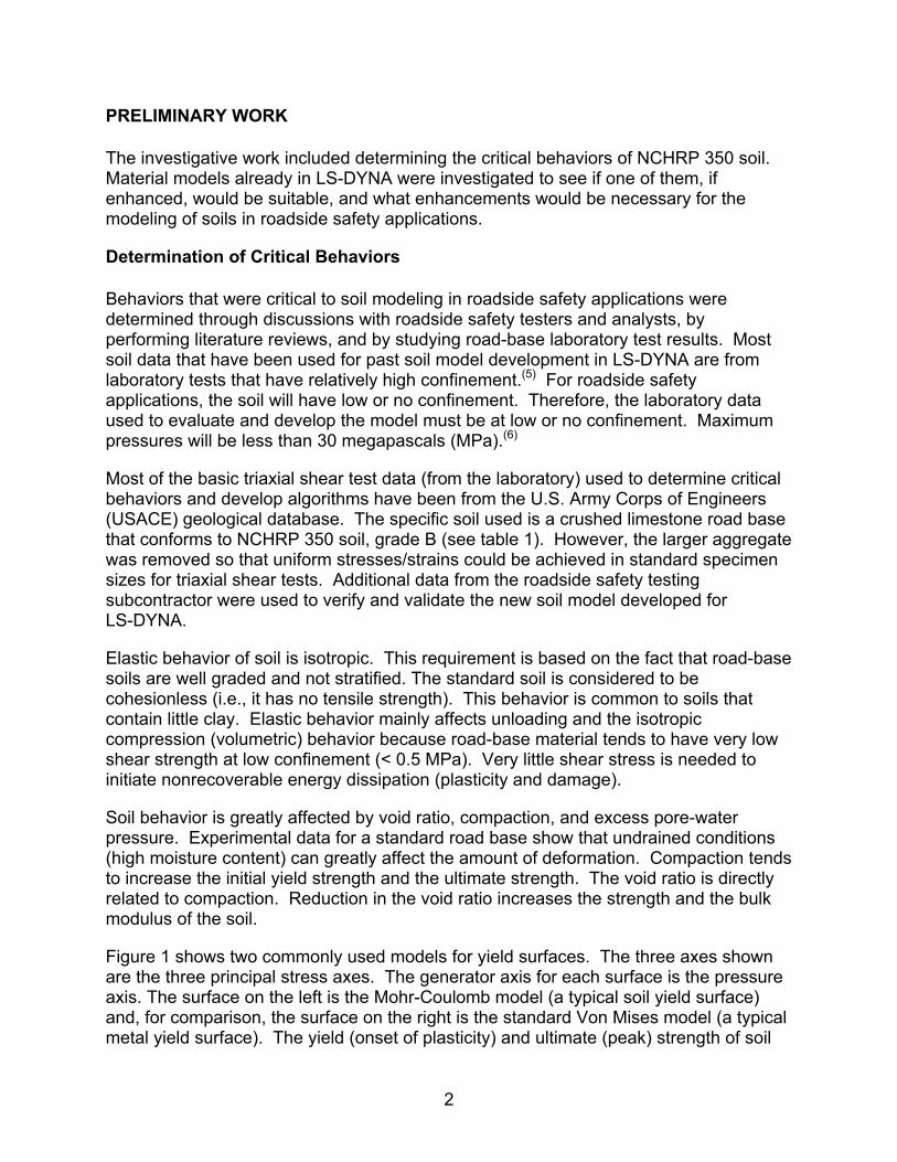
Table 1. Gradation data for USACE road-base soil tests.

Sieve Size (mm) Percent Passing

9.5200 100.0

6.3500 90.0

4.7600 79.0

3.3600 66.0

2.3800 54.0

2.0000 49.0

1.1900 36.0

0.8400 32.0

0.5900 28.0

0.4200 24.0

0.2970 21.0

0.2100 18.0

0.1490 15.0

0.1050 13.0

0.0740 11.0

4

(a) (b)

Figure 1. (a) Pressure-dependent (Mohr-Coulomb) and (b) pressure-independent (Von Mises) yield surfaces.

Figure 2. Yield surface in deviatoric plane for cohesionless soils.

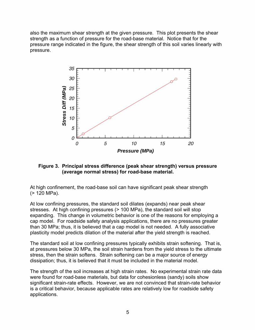
Figure 3 shows the peak principal stress difference versus the average normal stress for the crushed limestone road-base material. The peak principal stress difference is

σ3

Data From Monterey No. 0 SAND

σ2

σ1

5

also the maximum shear strength at the given pressure. This plot presents the shear strength as a function of pressure for the road-base material. Notice that for the pressure range indicated in the figure, the shear strength of this soil varies linearly with pressure.

Figure 3. Principal stress difference (peak shear strength) versus pressure (average normal stress) for road-base material.

At high confinement, the road-base soil can have significant peak shear strength (> 120 MPa).

At low confining pressures, the standard soil dilates (expands) near peak shear stresses. At high confining pressures (> 100 MPa), the standard soil will stop expanding. This change in volumetric behavior is one of the reasons for employing a cap model. For roadside safety analysis applications, there are no pressures greater than 30 MPa; thus, it is believed that a cap model is not needed. A fully associative plasticity model predicts dilation of the material after the yield strength is reached.

The standard soil at low confining pressures typically exhibits strain softening. That is, at pressures below 30 MPa, the soil strain hardens from the yield stress to the ultimate stress, then the strain softens. Strain softening can be a major source of energy dissipation; thus, it is believed that it must be included in the material model.

The strength of the soil increases at high strain rates. No experimental strain rate data were found for road-base materials, but data for cohesionless (sandy) soils show significant strain-rate effects. However, we are not convinced that strain-rate behavior is a critical behavior, because applicable rates are relatively low for roadside safety applications.

Stre

ss D

iff (M

Pa)

Pressure (MPa)

6

The moisture content of the soil can affect the elastic moduli, the shear strength, and the softening behavior of the soil.

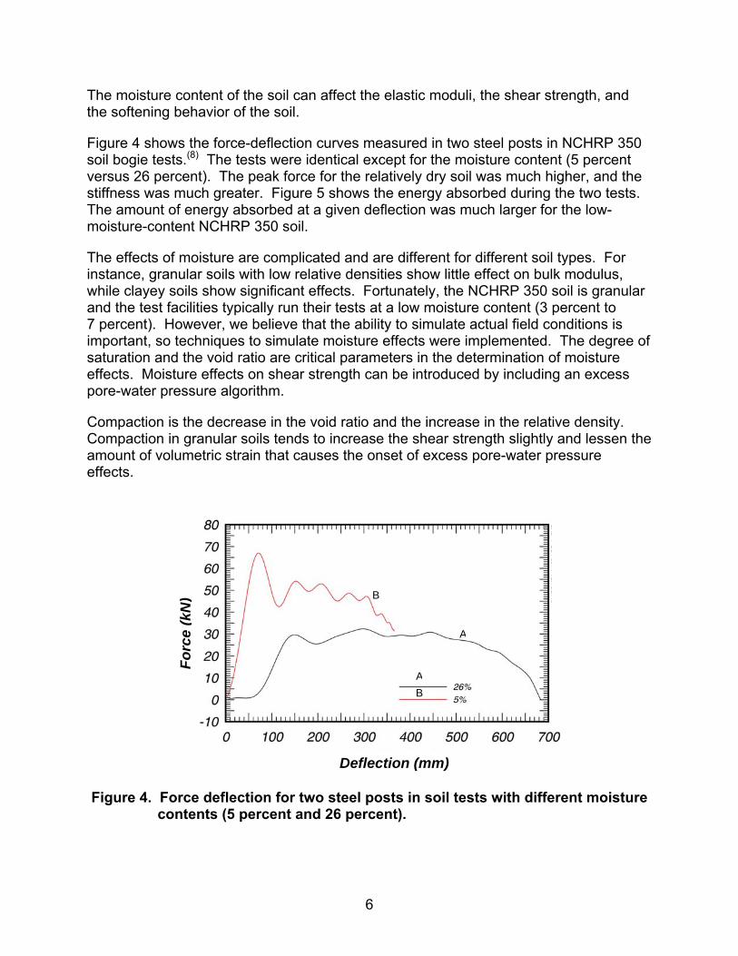
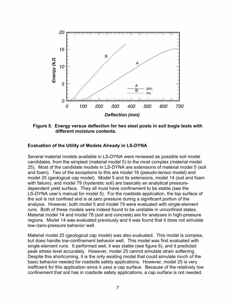
Figure 4 shows the force-deflection curves measured in two steel posts in NCHRP 350 soil bogie tests.(8) The tests were identical except for the moisture content (5 percent versus 26 percent). The peak force for the relatively dry soil was much higher, and the stiffness was much greater. Figure 5 shows the energy absorbed during the two tests. The amount of energy absorbed at a given deflection was much larger for the low-moisture-content NCHRP 350 soil.

The effects of moisture are complicated and are different for different soil types. For instance, granular soils with low relative densities show little effect on bulk modulus, while clayey soils show significant effects. Fortunately, the NCHRP 350 soil is granular and the test facilities typically run their tests at a low moisture content (3 percent to 7 percent). However, we believe that the ability to simulate actual field conditions is important, so techniques to simulate moisture effects were implemented. The degree of saturation and the void ratio are critical parameters in the determination of moisture effects. Moisture effects on shear strength can be introduced by including an excess pore-water pressure algorithm.

Compaction is the decrease in the void ratio and the increase in the relative density. Compaction in granular soils tends to increase the shear strength slightly and lessen the amount of volumetric strain that causes the onset of excess pore-water pressure effects.

Figure 4. Force deflection for two steel posts in soil tests with different moisture contents (5 percent and 26 percent).

AB

B

A

Forc

e (k

N)

Deflection (mm)

7

Figure 5. Energy versus deflection for two steel posts in soil bogie tests with different moisture contents.

Evaluation of the Utility of Models Already in LS-DYNA

Several material models available in LS-DYNA were reviewed as possible soil model candidates, from the simplest (material model 5) to the most complex (material model 25). Most of the candidate models in LS-DYNA are extensions of material model 5 (soil and foam). Two of the exceptions to this are model 16 (pseudo-tensor model) and model 25 (geological cap model). Model 5 and its extensions, model 14 (soil and foam with failure), and model 79 (hysteretic soil) are basically an analytical pressure-dependent yield surface. They all must have confinement to be stable (see the LS-DYNA user’s manual for model 5). For the roadside application, the top surface of the soil is not confined and is at zero pressure during a significant portion of the analysis. However, both model 5 and model 79 were evaluated with single-element runs. Both of these models were indeed found to be unstable in unconfined states. Material model 14 and model 78 (soil and concrete) are for analyses in high-pressure regions. Model 14 was evaluated previously and it was found that it does not simulate low-/zero-pressure behavior well.

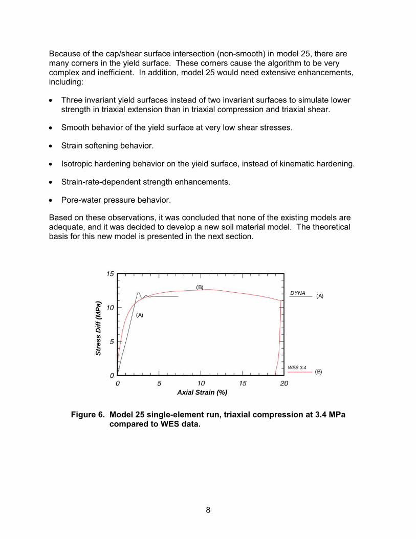
Material model 25 (geological cap model) was also evaluated. This model is complex, but does handle low-confinement behavior well. This model was first evaluated with single-element runs. It performed well, it was stable (see figure 6), and it predicted peak stress level accurately. However, model 25 cannot simulate strain softening. Despite this shortcoming, it is the only existing model that could simulate much of the basic behavior needed for roadside safety applications. However, model 25 is very inefficient for this application since it uses a cap surface. Because of the relatively low confinement that soil has in roadside safety applications, a cap surface is not needed.

Ener

gy (k

J)

AB

B

A

Deflection (mm)

8

Because of the cap/shear surface intersection (non-smooth) in model 25, there are many corners in the yield surface. These corners cause the algorithm to be very complex and inefficient. In addition, model 25 would need extensive enhancements, including:

• Three invariant yield surfaces instead of two invariant surfaces to simulate lower strength in triaxial extension than in triaxial compression and triaxial shear.

• Smooth behavior of the yield surface at very low shear stresses.

• Strain softening behavior.

• Isotropic hardening behavior on the yield surface, instead of kinematic hardening.

• Strain-rate-dependent strength enhancements.

• Pore-water pressure behavior.

Based on these observations, it was concluded that none of the existing models are adequate, and it was decided to develop a new soil material model. The theoretical basis for this new model is presented in the next section.

Figure 6. Model 25 single-element run, triaxial compression at 3.4 MPa compared to WES data.

Axial Strain (%)

(A)

(A)

(B)

(B)DYNA

Stre

ss D

iff (M

Pa)

9

MODEL DEVELOPMENT

The objectives of the material model development effort in order of priority were: accuracy, robustness, efficiency (speed), and ease of use. The choices made in the model are balanced between these objectives. The following subsections describe the characteristics of the algorithms necessary to model soil for roadside safety applications.

Elastic Constitutive Behavior

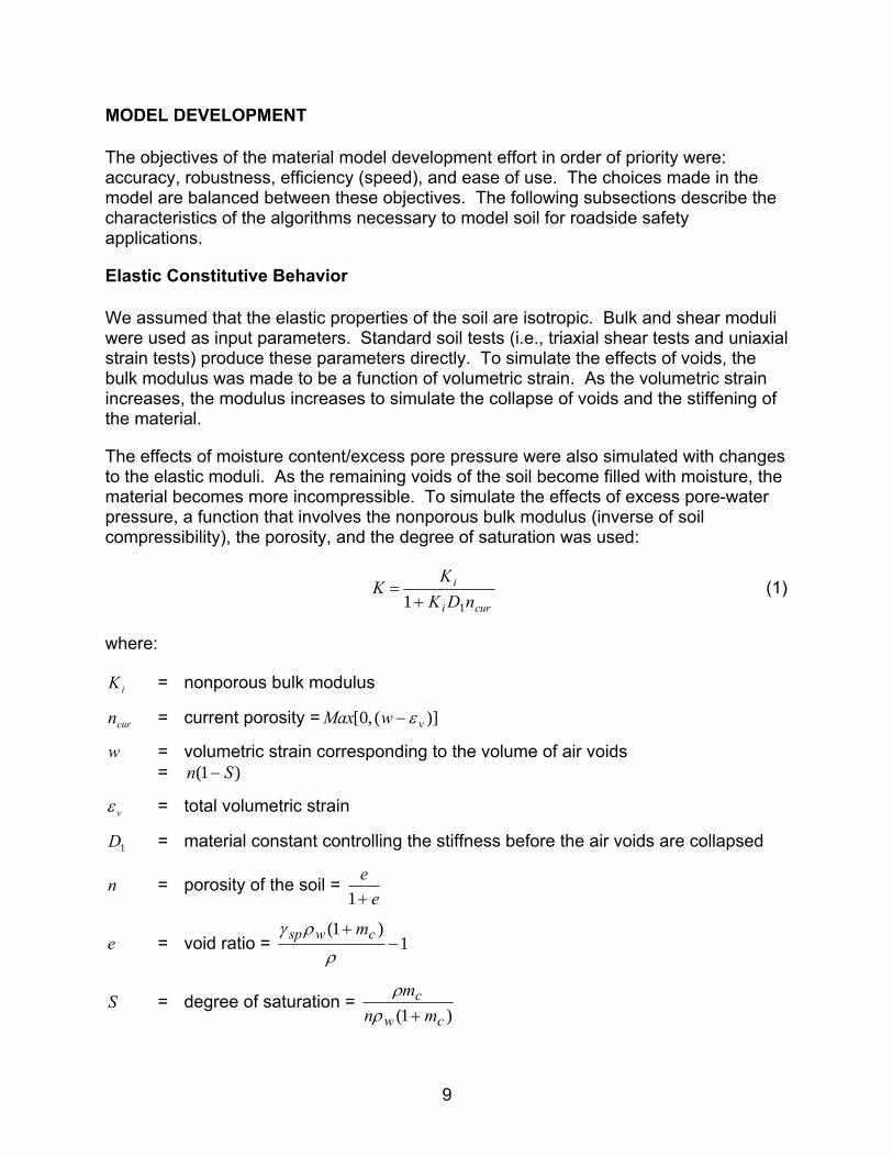
We assumed that the elastic properties of the soil are isotropic. Bulk and shear moduli were used as input parameters. Standard soil tests (i.e., triaxial shear tests and uniaxial strain tests) produce these parameters directly. To simulate the effects of voids, the bulk modulus was made to be a function of volumetric strain. As the volumetric strain increases, the modulus increases to simulate the collapse of voids and the stiffening of the material.

The effects of moisture content/excess pore pressure were also simulated with changes to the elastic moduli. As the remaining voids of the soil become filled with moisture, the material becomes more incompressible. To simulate the effects of excess pore-water pressure, a function that involves the nonporous bulk modulus (inverse of soil compressibility), the porosity, and the degree of saturation was used:

curi

i

nDKK

K11 +

= (1)

where:

iK = nonporous bulk modulus

curn = current porosity = )](,0[ vwMax ε−

w = volumetric strain corresponding to the volume of air voids = )1( Sn −

vε = total volumetric strain

1D = material constant controlling the stiffness before the air voids are collapsed

n = porosity of the soil = e

e+1

e = void ratio = 1)1(

−+

ρ

ργ cwsp m

S = degree of saturation = )1( cw

cmn

m+ρ

ρ

10

wcsp m,γρ, ρ, = soil density, specific gravity, moisture content, and water density.

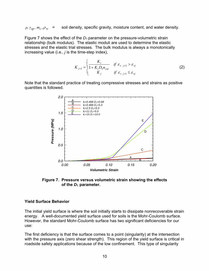
Figure 7 shows the effect of the D1 parameter on the pressure-volumetric strain relationship (bulk modulus). The elastic moduli are used to determine the elastic stresses and the elastic trial stresses. The bulk modulus is always a monotonically increasing value (i.e., j is the time-step index),

⎪⎩

⎪⎨⎧

≤

>+=

+

++

vjjvj

vjjvcuri

i

jifK

ifnDK

KK

εε

εε

1

111 1 (2)

Note that the standard practice of treating compressive stresses and strains as positive quantities is followed.

Figure 7. Pressure versus volumetric strain showing the effects of the D1 parameter.

Yield Surface Behavior

The initial yield surface is where the soil initially starts to dissipate nonrecoverable strain energy. A well-documented yield surface used for soils is the Mohr-Coulomb surface. However, the standard Mohr-Coulomb surface has two significant deficiencies for our use:

The first deficiency is that the surface comes to a point (singularity) at the intersection with the pressure axis (zero shear strength). This region of the yield surface is critical in roadside safety applications because of the low confinement. This type of singularity

A

A

B

B

C

C

D

D

E

E

ki=0.468 D1=0.68 ki=0.468 D1=5.0 ki=2.5 D1=5.0 ki=11 D1=5.0 ki=15 D1=10.0

Volumetric Strain

Pres

sure

(MPa

)

Volumetric Strain

11

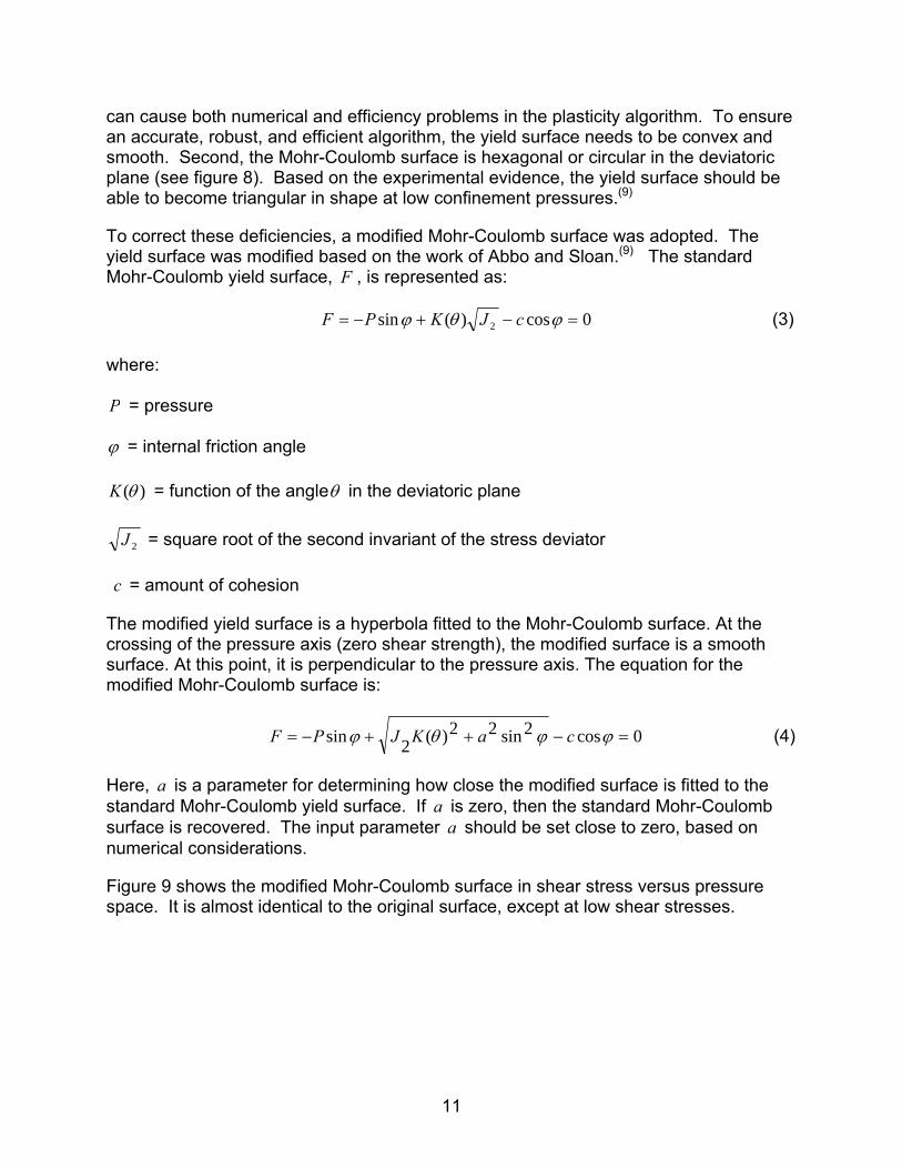
can cause both numerical and efficiency problems in the plasticity algorithm. To ensure an accurate, robust, and efficient algorithm, the yield surface needs to be convex and smooth. Second, the Mohr-Coulomb surface is hexagonal or circular in the deviatoric plane (see figure 8). Based on the experimental evidence, the yield surface should be able to become triangular in shape at low confinement pressures.(9)

To correct these deficiencies, a modified Mohr-Coulomb surface was adopted. The yield surface was modified based on the work of Abbo and Sloan.(9) The standard Mohr-Coulomb yield surface, F , is represented as:

0cos)(sin 2 =−+−= ϕθϕ cJKPF (3) where: P = pressure ϕ = internal friction angle

)(θK = function of the angleθ in the deviatoric plane

2J = square root of the second invariant of the stress deviator c = amount of cohesion

The modified yield surface is a hyperbola fitted to the Mohr-Coulomb surface. At the crossing of the pressure axis (zero shear strength), the modified surface is a smooth surface. At this point, it is perpendicular to the pressure axis. The equation for the modified Mohr-Coulomb surface is:

0cos2sin22)(2sin =−++−= ϕϕθϕ caKJPF (4)

Here, a is a parameter for determining how close the modified surface is fitted to the standard Mohr-Coulomb yield surface. If a is zero, then the standard Mohr-Coulomb surface is recovered. The input parameter a should be set close to zero, based on numerical considerations.

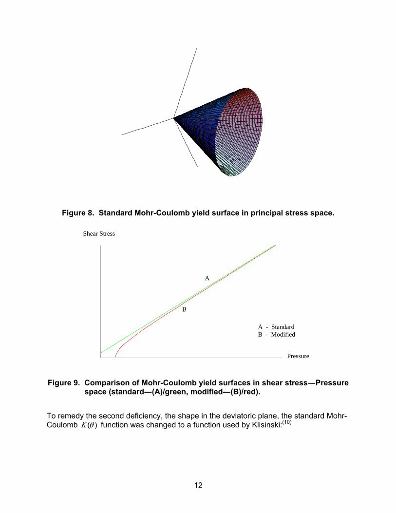
Figure 9 shows the modified Mohr-Coulomb surface in shear stress versus pressure space. It is almost identical to the original surface, except at low shear stresses.

12

Figure 8. Standard Mohr-Coulomb yield surface in principal stress space.

Pressure

Shear Stress

Figure 9. Comparison of Mohr-Coulomb yield surfaces in shear stress―Pressure space (standard―(A)/green, modified―(B)/red).

To remedy the second deficiency, the shape in the deviatoric plane, the standard Mohr-Coulomb )(θK function was changed to a function used by Klisinski:(10)

A - Standard B - Modified

A

B

Shear Stress

Pressure

13

21

2222

222

]45cos)1(4)[12(cos)1(2

)12(cos)1(4)(eeeee

eeK−+−−+−

−+−=

θθ

θθ (5)

Here, 2

3

2

3

J2

J333cos =θ , 3J = third invariant of the stress deviator, and e = material input

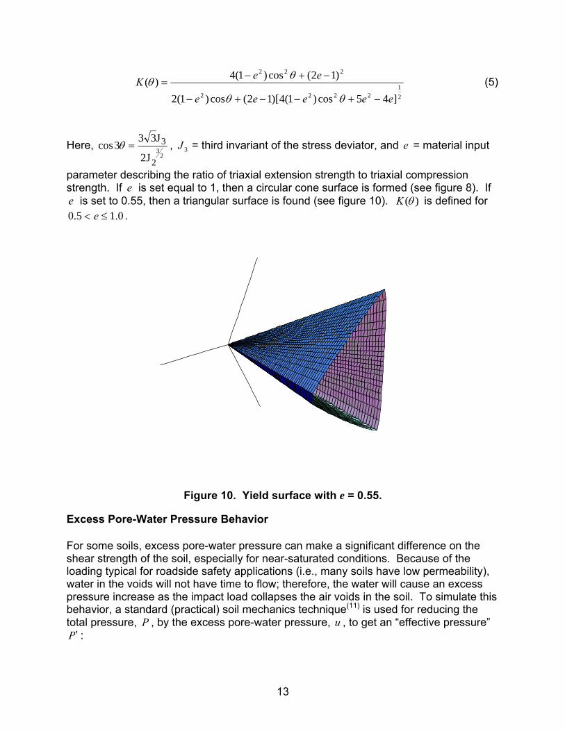
parameter describing the ratio of triaxial extension strength to triaxial compression strength. If e is set equal to 1, then a circular cone surface is formed (see figure 8). If e is set to 0.55, then a triangular surface is found (see figure 10). )(θK is defined for

0.15.0 ≤< e .

Figure 10. Yield surface with e = 0.55.

Excess Pore-Water Pressure Behavior

For some soils, excess pore-water pressure can make a significant difference on the shear strength of the soil, especially for near-saturated conditions. Because of the loading typical for roadside safety applications (i.e., many soils have low permeability), water in the voids will not have time to flow; therefore, the water will cause an excess pressure increase as the impact load collapses the air voids in the soil. To simulate this behavior, a standard (practical) soil mechanics technique(11) is used for reducing the total pressure, P , by the excess pore-water pressure, u , to get an “effective pressure” P′ :

14

uPP −=′ (6)

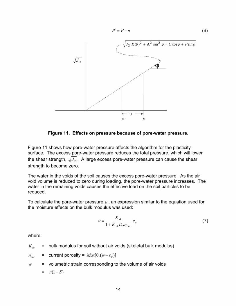
Figure 11. Effects on pressure because of pore-water pressure.

Figure 11 shows how pore-water pressure affects the algorithm for the plasticity surface. The excess pore-water pressure reduces the total pressure, which will lower the shear strength, 2J . A large excess pore-water pressure can cause the shear strength to become zero.

The water in the voids of the soil causes the excess pore-water pressure. As the air void volume is reduced to zero during loading, the pore-water pressure increases. The water in the remaining voids causes the effective load on the soil particles to be reduced.

To calculate the pore-water pressure,u , an expression similar to the equation used for the moisture effects on the bulk modulus was used:

vcursk

sk

nDKK

u ε21 +

= (7)

where:

skK = bulk modulus for soil without air voids (skeletal bulk modulus)

curn = current porosity = )](,0[ vwMax ε−

w = volumetric strain corresponding to the volume of air voids

= )1( Sn −

ϕϕϕθ sincossinA)( 2222 PCKJ +=+

15

vε = total volumetric strain

2D = material constant controlling the pore-water pressure before the air voids are collapsed

n = porosity of the soil = e

e+1

e = void ratio = 1)1(

−+

ργ csp m

S = degree of saturation = )1( c

c

mnm+

ρ

csp m,, γρ = soil density, specific gravity, and moisture content, respectively

Pore-water pressure is not allowed to become negative ( 0≥u ).

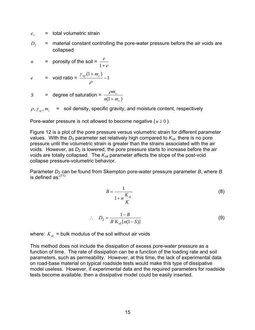
Figure 12 is a plot of the pore pressure versus volumetric strain for different parameter values. With the D2 parameter set relatively high compared to Ksk, there is no pore pressure until the volumetric strain is greater than the strains associated with the air voids. However, as D2 is lowered, the pore pressure starts to increase before the air voids are totally collapsed. The Ksk parameter affects the slope of the post-void collapse pressure-volumetric behavior.

Parameter D2 can be found from Skempton pore-water pressure parameter B, where B is defined as:(11)

KKn

Bsk+

=1

1 (8)

)]1([1

2 SnKBBD

sk −−

=∴ (9)

where: skK = bulk modulus of the soil without air voids

This method does not include the dissipation of excess pore-water pressure as a function of time. The rate of dissipation can be a function of the loading rate and soil parameters, such as permeability. However, at this time, the lack of experimental data on road-base material on typical roadside tests would make this type of dissipative model useless. However, if experimental data and the required parameters for roadside tests become available, then a dissipative model could be easily inserted.

16

Figure 12. Effects of parameters on pore-water pressure.

Strain Hardening Behavior

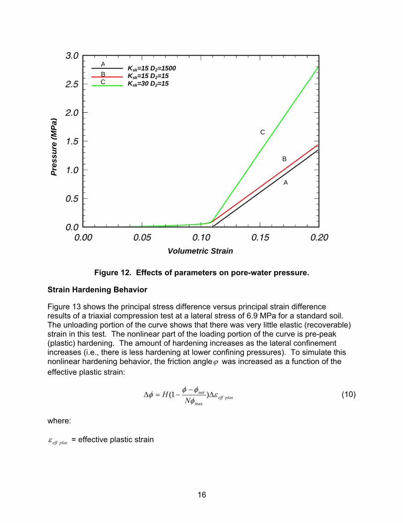
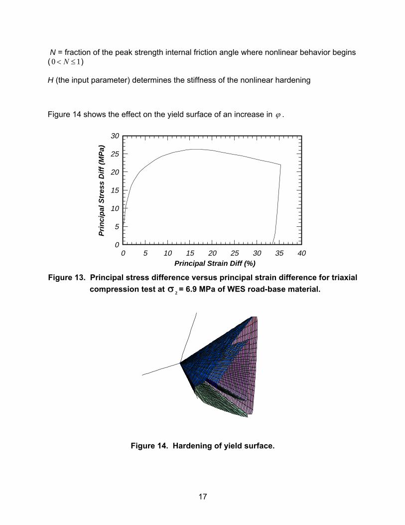
Figure 13 shows the principal stress difference versus principal strain difference results of a triaxial compression test at a lateral stress of 6.9 MPa for a standard soil. The unloading portion of the curve shows that there was very little elastic (recoverable) strain in this test. The nonlinear part of the loading portion of the curve is pre-peak (plastic) hardening. The amount of hardening increases as the lateral confinement increases (i.e., there is less hardening at lower confining pressures). To simulate this nonlinear hardening behavior, the friction angleϕ was increased as a function of the effective plastic strain:

plaseffinit

NH ε

φφφφ ∆

−−=∆ )1(

max

(10)

where:

plaseffε = effective plastic strain

Volumetric Strain

A B

A

C

B

C

Ksk=15 D2=1500 Ksk=15 D2=15 Ksk=30 D2=15

Pres

sure

(MPa

)

17

N = fraction of the peak strength internal friction angle where nonlinear behavior begins ( 10 ≤< N ) H (the input parameter) determines the stiffness of the nonlinear hardening

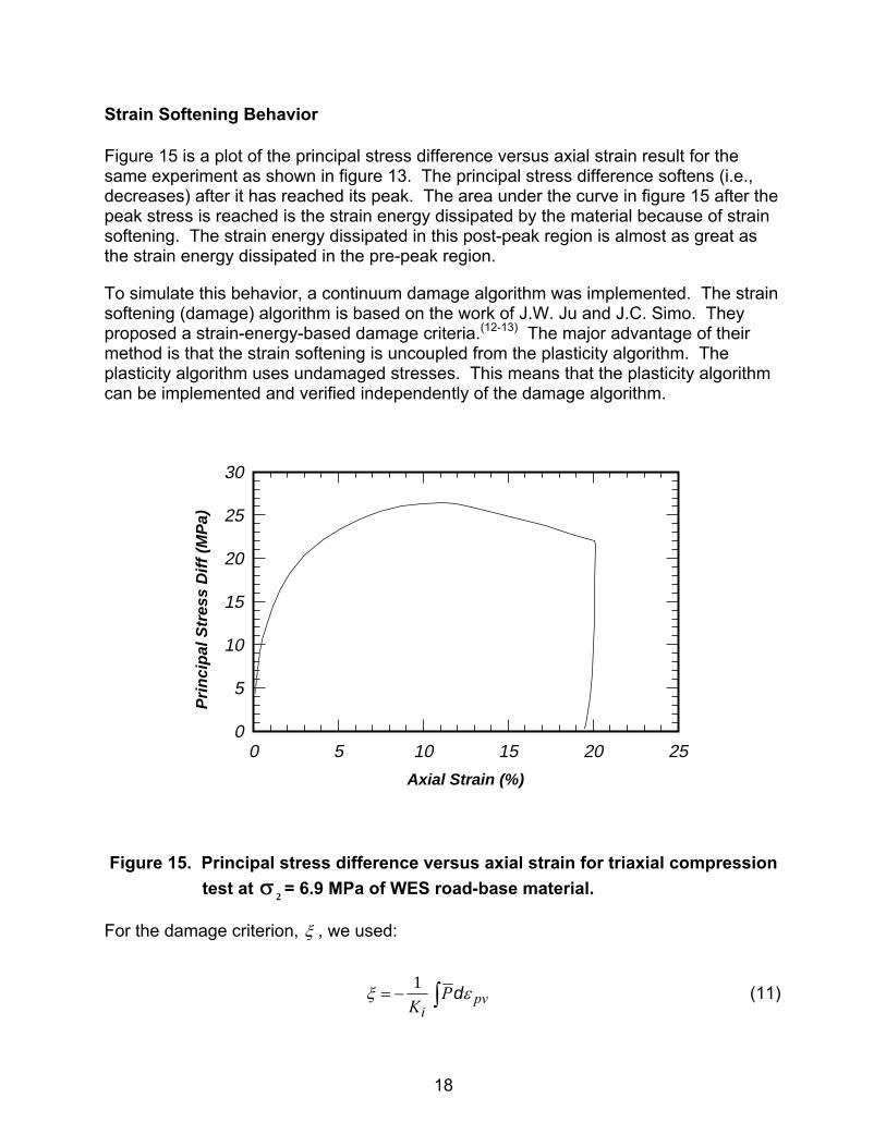
Figure 14 shows the effect on the yield surface of an increase in ϕ .

BA

L 4-MA

R-99 A

PT

EK

DE

146

0 5 10 15 20 25 30 35 400

5

10

15

20

25

30

Principal Strain Diff %

Prin

cipa

l Str

ess

Diff

MP

a

Figure 13. Principal stress difference versus principal strain difference for triaxial

compression test at 2σ = 6.9 MPa of WES road-base material.

Figure 14. Hardening of yield surface.

Principal Strain Diff (%)

Prin

cipa

l Str

ess

Diff

(MPa

)

18

Strain Softening Behavior

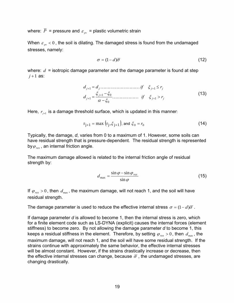
Figure 15 is a plot of the principal stress difference versus axial strain result for the same experiment as shown in figure 13. The principal stress difference softens (i.e., decreases) after it has reached its peak. The area under the curve in figure 15 after the peak stress is reached is the strain energy dissipated by the material because of strain softening. The strain energy dissipated in this post-peak region is almost as great as the strain energy dissipated in the pre-peak region.

To simulate this behavior, a continuum damage algorithm was implemented. The strain softening (damage) algorithm is based on the work of J.W. Ju and J.C. Simo. They proposed a strain-energy-based damage criteria.(12-13) The major advantage of their method is that the strain softening is uncoupled from the plasticity algorithm. The plasticity algorithm uses undamaged stresses. This means that the plasticity algorithm can be implemented and verified independently of the damage algorithm.

BA

L 4-MA

R-99 A

PT

EK

FH

WA

0 5 10 15 20 250

5

10

15

20

25

30

Axial Strain %

Prin

cipa

l Str

ess

Diff

MP

a

Figure 15. Principal stress difference versus axial strain for triaxial compression test at 2σ = 6.9 MPa of WES road-base material.

For the damage criterion, ξ , we used:

∫−= pvi

PK

εξ d1 (11)

Axial Strain (%)

Prin

cipa

l Str

ess

Diff

(MPa

)

19

where: P = pressure and pvε = plastic volumetric strain

When 0<pvε , the soil is dilating. The damaged stress is found from the undamaged stresses, namely:

σσ )1( d−= (12)

where: d = isotropic damage parameter and the damage parameter is found at step 1+j as:

jjj

j

jjjj

rifd

rifdd

>−−

=

≤=

++

+

++

10

011

11

ξξαξξ

ξ

KKKKKK

KKKKKKKKK

(13)

Here, 1+jr is a damage threshold surface, which is updated in this manner:

( )1jj1j ,rmaxr ++ = ξ , and 00 r=ξ (14)

Typically, the damage, d, varies from 0 to a maximum of 1. However, some soils can have residual strength that is pressure-dependent. The residual strength is represented by resϕ , an internal friction angle.

The maximum damage allowed is related to the internal friction angle of residual strength by:

ϕϕϕ

sinsinsin

maxresd

−= (15)

If 0>resϕ , then maxd , the maximum damage, will not reach 1, and the soil will have residual strength. The damage parameter is used to reduce the effective internal stress σσ )1( d−= . If damage parameter d is allowed to become 1, then the internal stress is zero, which for a finite element code such as LS-DYNA (explicit) causes the internal forces (element stiffness) to become zero. By not allowing the damage parameter d to become 1, this keeps a residual stiffness in the element. Therefore, by setting 0>resϕ , then maxd , the maximum damage, will not reach 1, and the soil will have some residual strength. If the strains continue with approximately the same behavior, the effective internal stresses will be almost constant. However, if the strains drastically increase or decrease, then the effective internal stresses can change, because σ , the undamaged stresses, are changing drastically.

20

When material models include strain softening, special techniques must be used to prevent mesh sensitivity. Mesh sensitivity is the tendency of the finite element model/analysis to produce significantly different results as the element size is reduced. Mesh sensitivity occurs because softening in the model concentrates in one element. As the element size is reduced, the failure becomes localized in smaller volumes; this causes less energy to be dissipated by the softening, leading to instabilities or at least mesh-sensitive behavior.

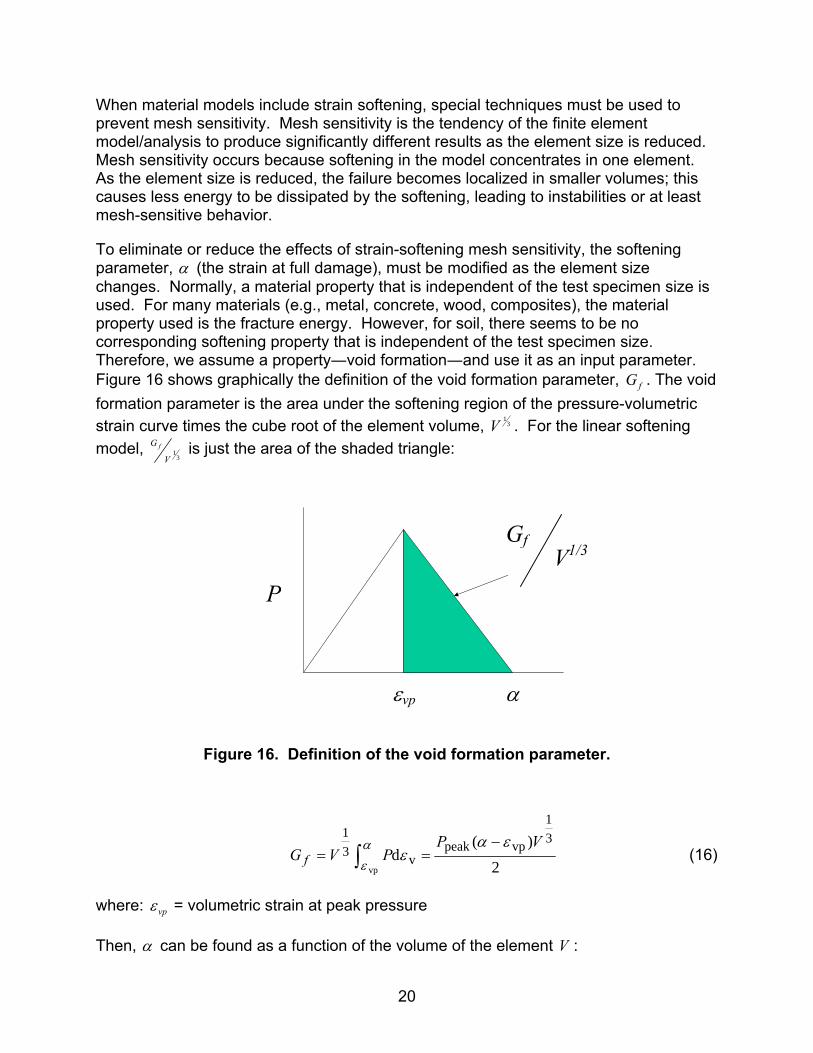
To eliminate or reduce the effects of strain-softening mesh sensitivity, the softening parameter, α (the strain at full damage), must be modified as the element size changes. Normally, a material property that is independent of the test specimen size is used. For many materials (e.g., metal, concrete, wood, composites), the material property used is the fracture energy. However, for soil, there seems to be no corresponding softening property that is independent of the test specimen size. Therefore, we assume a property―void formation―and use it as an input parameter. Figure 16 shows graphically the definition of the void formation parameter, fG . The void formation parameter is the area under the softening region of the pressure-volumetric strain curve times the cube root of the element volume, 3

1V . For the linear softening model,

31

V

G f is just the area of the shaded triangle:

vpε

31

V

Gf

P

α

Figure 16. Definition of the void formation parameter.

2)(

d31

vppeakv3

1

vp

VPPVG f

εαε

αε

−== ∫ (16)

where: vpε = volumetric strain at peak pressure

Then, α can be found as a function of the volume of the element V :

P

GfV1/3

εvp α

21

vp

vp

f

VK

Gε

εα +=

31

2 (17)

where: vpε = an input parameter

If fG is made very small relative to 31

VK vpε , then the softening behavior will be brittle.

Strain-Rate Behavior

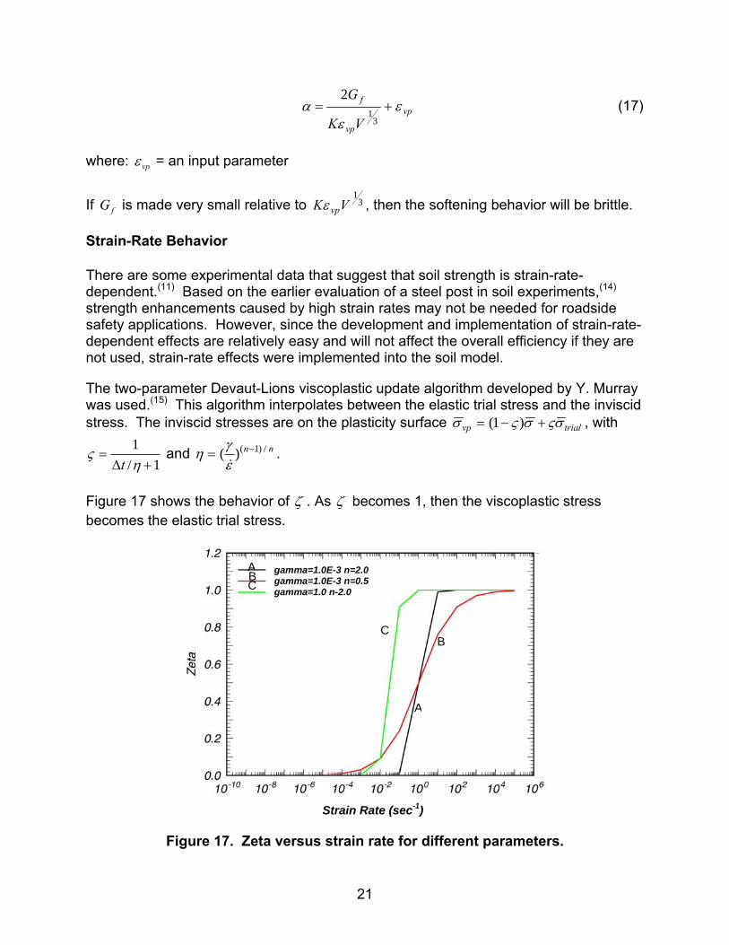
There are some experimental data that suggest that soil strength is strain-rate-dependent.(11) Based on the earlier evaluation of a steel post in soil experiments,(14) strength enhancements caused by high strain rates may not be needed for roadside safety applications. However, since the development and implementation of strain-rate-dependent effects are relatively easy and will not affect the overall efficiency if they are not used, strain-rate effects were implemented into the soil model.

The two-parameter Devaut-Lions viscoplastic update algorithm developed by Y. Murray was used.(15) This algorithm interpolates between the elastic trial stress and the inviscid stress. The inviscid stresses are on the plasticity surface trialvp σςσςσ +−= )1( , with

1/1

+∆=

ης

t and nn /)1()( −=

εγη&

.

Figure 17 shows the behavior of ζ . As ζ becomes 1, then the viscoplastic stress becomes the elastic trial stress.

Figure 17. Zeta versus strain rate for different parameters.

A

BC

C B A gamma=1.0E-3 n=2.0

gamma=1.0E-3 n=0.5gamma=1.0 n-2.0

Strain Rate (sec-1)

22

INCORPORATION INTO LS-DYNA

The above discussion describes the equations and the form of the soil model. In this section, the implementation of the model into LS-DYNA is discussed. The intermediate equations were determined using the symbolic algebra program Mathematica®.

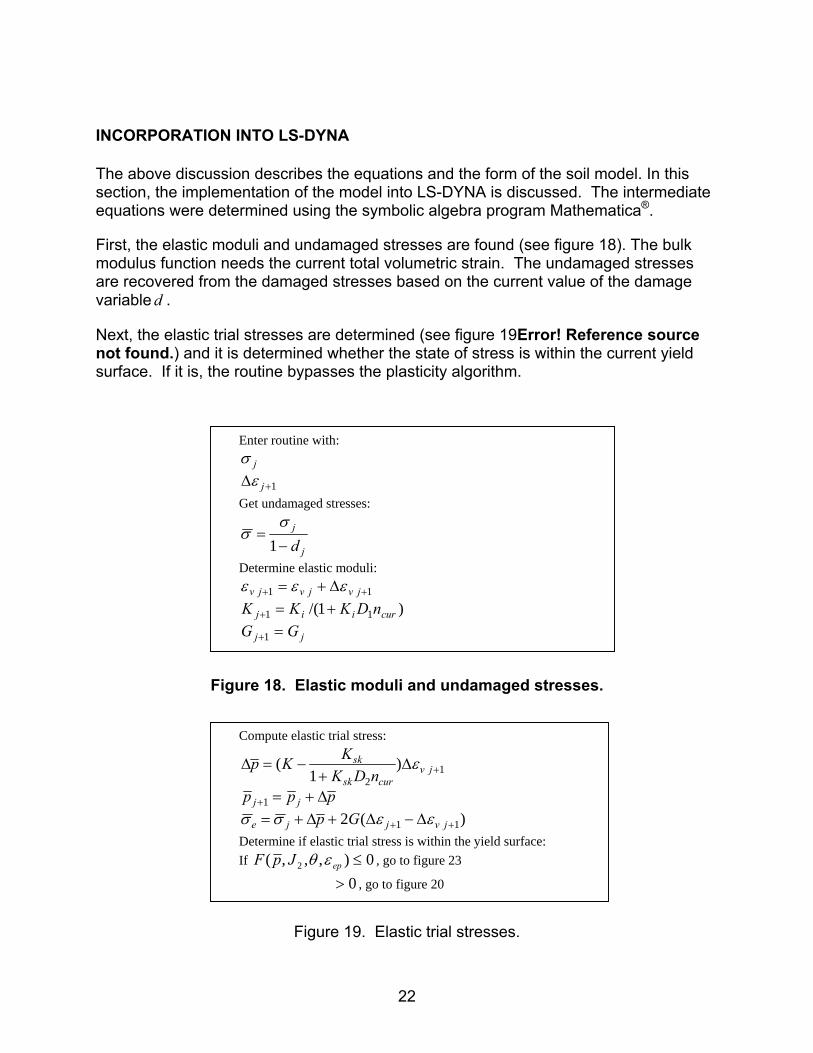
First, the elastic moduli and undamaged stresses are found (see figure 18). The bulk modulus function needs the current total volumetric strain. The undamaged stresses are recovered from the damaged stresses based on the current value of the damage variable d .

Next, the elastic trial stresses are determined (see figure 19Error! Reference source not found.) and it is determined whether the state of stress is within the current yield surface. If it is, the routine bypasses the plasticity algorithm.

Figure 18. Elastic moduli and undamaged stresses.

Figure 19. Elastic trial stresses.

Enter routine with:

1+∆ j

j

εσ

Get undamaged stresses:

j

j

d−=

1σ

σ

Determine elastic moduli:

jj

curiij

jvjvjv

GGnDKKK

=+=∆+=

+

+

++

1

11

11

)1/(εεε

Compute elastic trial stress:

)(2

)1

(

11

1

12

++

+

+

∆−∆+∆+=∆+=

∆+

−=∆

jvjje

jj

jvcursk

sk

Gpppp

nDKKKp

εεσσ

ε

Determine if elastic trial stress is within the yield surface: If 0),,,( 2 ≤epJpF εθ , go to figure 23

0> , go to figure 20

23

The total strains are split into elastic and plastic strains:

pe εεε += (18) The stress increment at step 1+j is then:

)( 111 +++ ∆−∆=∆ jpjj C εεσ (19) To compute the stress increments, it is first necessary to determine the plastic strain increments. The latter are determined by assuming an associated flow rule (see figure 20). Note that the gradient of the yield function is taken at the stress state of the previous time step; this is consistent with the explicit algorithm used in LS-DYNA. The explicit form of the gradients is presented in appendix A. The increment in the hardening parameter ϕ is assumed to have a form similar to the flow rule. C is the elasticity tensor. The function h will be determined later (see figure 21). For the determination of the increment of the scale parameter, the gradients of the yield function are again evaluated at step j. Once the plasticity scale parameter is determined, the stresses and history variables can be updated (see figure 21).

Figure 20. Determination of plastic strains.

The plastic strain increment is found from the associated flow rule:

jjp

Fσ

λε∂∂

∆=∆ + 1

The increment in the hardening parameter ϕ is:

)( eph ελϕ ∆=∆

Employing standard techniques, the increment of the scalar parameter λ is:

hFFCF

CF

ϕσσ

εσλ

∂∂

−∂∂

∂∂

∆∂∂

=∆

24

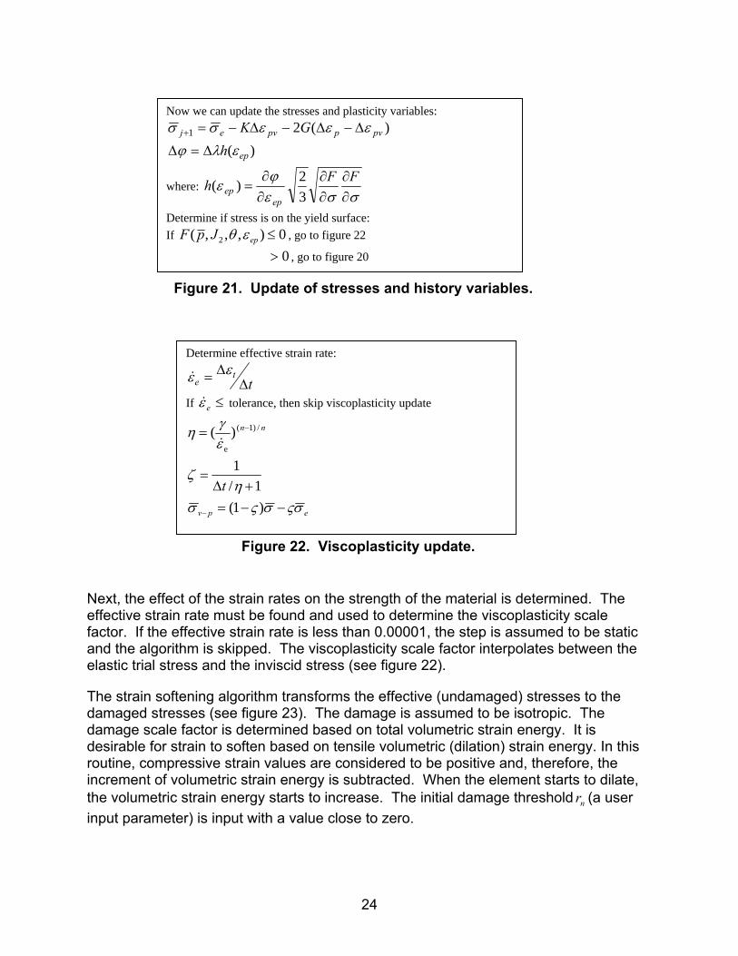
Figure 21. Update of stresses and history variables.

Figure 22. Viscoplasticity update.

Next, the effect of the strain rates on the strength of the material is determined. The effective strain rate must be found and used to determine the viscoplasticity scale factor. If the effective strain rate is less than 0.00001, the step is assumed to be static and the algorithm is skipped. The viscoplasticity scale factor interpolates between the elastic trial stress and the inviscid stress (see figure 22).

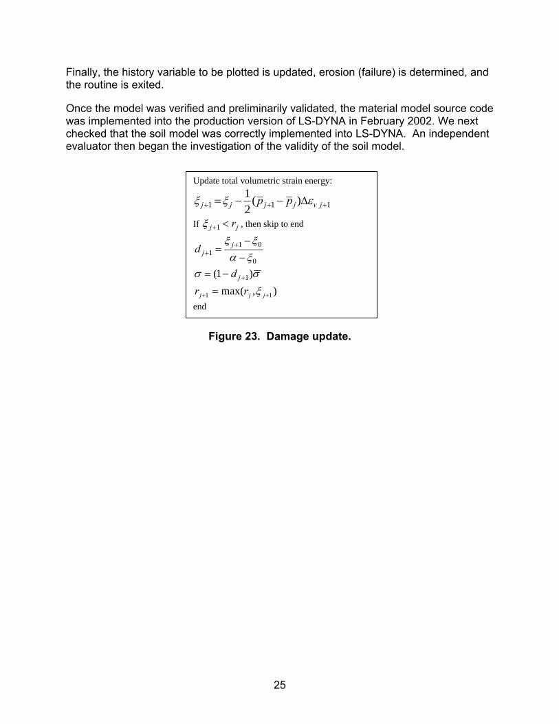
The strain softening algorithm transforms the effective (undamaged) stresses to the damaged stresses (see figure 23). The damage is assumed to be isotropic. The damage scale factor is determined based on total volumetric strain energy. It is desirable for strain to soften based on tensile volumetric (dilation) strain energy. In this routine, compressive strain values are considered to be positive and, therefore, the increment of volumetric strain energy is subtracted. When the element starts to dilate, the volumetric strain energy starts to increase. The initial damage threshold nr (a user input parameter) is input with a value close to zero.

Determine effective strain rate:

tt

e ∆∆= εε&

If ≤eε& tolerance, then skip viscoplasticity update

epv

nn

tσςσςσ

ηζ

εγη

−−=+∆

=

=

−

−

)1(1/

1

)( /)1(

e&

Now we can update the stresses and plasticity variables: )(21 pvppvej GK εεεσσ ∆−∆−∆−=+

)( eph ελϕ ∆=∆

where: σσε

ϕε

∂∂

∂∂

∂∂

=FFh

epep 3

2)(

Determine if stress is on the yield surface: If 0),,,( 2 ≤epJpF εθ , go to figure 22

0> , go to figure 20

25

Finally, the history variable to be plotted is updated, erosion (failure) is determined, and the routine is exited.

Once the model was verified and preliminarily validated, the material model source code was implemented into the production version of LS-DYNA in February 2002. We next checked that the soil model was correctly implemented into LS-DYNA. An independent evaluator then began the investigation of the validity of the soil model.

Figure 23. Damage update.

Update total volumetric strain energy:

111 )(21

+++ ∆−−= jvjjjj pp εξξ

If jj r<+1ξ , then skip to end

0

011 ξα

ξξ−−

= ++

jjd

σσ )1( 1+−= jd

),max( 11 ++ = jjj rr ξ end

27

CHAPTER 2. USER’S MANUAL

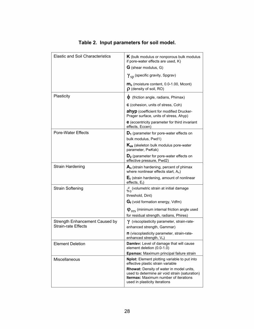
The user’s manual was written as the model was being implemented, verified, and validated. The user’s manual consists of a user input guide (much like material model sections in the LS-DYNA user’s manual); a brief theory manual (LSTC theory manual), which is a condensed version of the first section of this report; and a discussion of the use of the model. Both manuals will be added to an updated LS-DYNA manual. The user’s manual addresses the basics of the model, input parameters, and basic equations. Table 2 contains a brief description of the user input variables for the soil model, along with the corresponding symbols used in the LSTC theory manual. The bold text is the LSTC theory manual symbol, which is typically followed by a brief description and then the user input value symbol. The parameters that need to be specified are dependent on the soil and the specific application.

28

Table 2. Input parameters for soil model.

Elastic and Soil Characteristics K (bulk modulus or nonporous bulk modulus if pore-water effects are used, K)

G (shear modulus, G)

spγ (specific gravity, Spgrav)

mc (moisture content, 0.0-1.00, Mcont) ρ (density of soil, RO)

Plasticity φ (friction angle, radians, Phimax)

c (cohesion, units of stress, Coh)

ahyp (coefficient for modified Drucker-Prager surface, units of stress, Ahyp)

e (eccentricity parameter for third invariant effects, Eccen)

Pore-Water Effects D1 (parameter for pore-water effects on bulk modulus, Pwd1)

Ksk (skeleton bulk modulus pore-water parameter, PwKsk)

D2 (parameter for pore-water effects on effective pressure, Pwd2)

Strain Hardening An (strain hardening, percent of phimax where nonlinear effects start, An)

Et (strain hardening, amount of nonlinear effects, Et)

Strain Softening 0ξ (volumetric strain at initial damage

threshold, Dint)

Gf (void formation energy, Vdfm)

resϕ (minimum internal friction angle used for residual strength, radians, Phires)

Strength Enhancement Caused by Strain-rate Effects

γ (viscoplasticity parameter, strain-rate-enhanced strength, Gammar)

n (viscoplasticity parameter, strain-rate-enhanced strength, Vn)

Element Deletion Damlev: Level of damage that will cause element deletion (0.0-1.0) Epsmax: Maximum principal failure strain

Miscellaneous Nplot: Element plotting variable to put into effective plastic strain variable Rhowat: Density of water in model units, used to determine air void strain (saturation) Itermax: Maximum number of iterations used in plasticity iterations

29

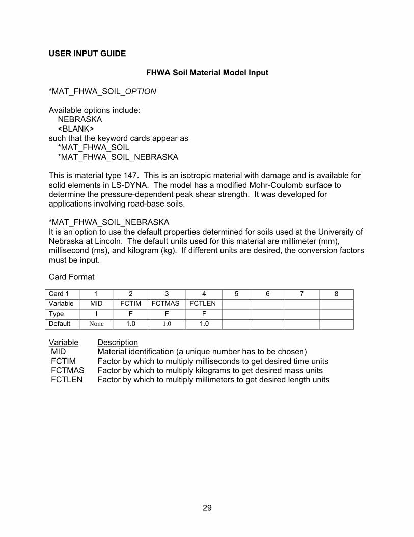
USER INPUT GUIDE

FHWA Soil Material Model Input

*MAT_FHWA_SOIL_OPTION Available options include: NEBRASKA <BLANK> such that the keyword cards appear as *MAT_FHWA_SOIL *MAT_FHWA_SOIL_NEBRASKA This is material type 147. This is an isotropic material with damage and is available for solid elements in LS-DYNA. The model has a modified Mohr-Coulomb surface to determine the pressure-dependent peak shear strength. It was developed for applications involving road-base soils. *MAT_FHWA_SOIL_NEBRASKA It is an option to use the default properties determined for soils used at the University of Nebraska at Lincoln. The default units used for this material are millimeter (mm), millisecond (ms), and kilogram (kg). If different units are desired, the conversion factors must be input. Card Format Card 1 1 2 3 4 5 6 7 8 Variable MID FCTIM FCTMAS FCTLEN Type I F F F Default None 1.0 1.0 1.0 Variable Description MID Material identification (a unique number has to be chosen) FCTIM Factor by which to multiply milliseconds to get desired time units FCTMAS Factor by which to multiply kilograms to get desired mass units FCTLEN Factor by which to multiply millimeters to get desired length units

30

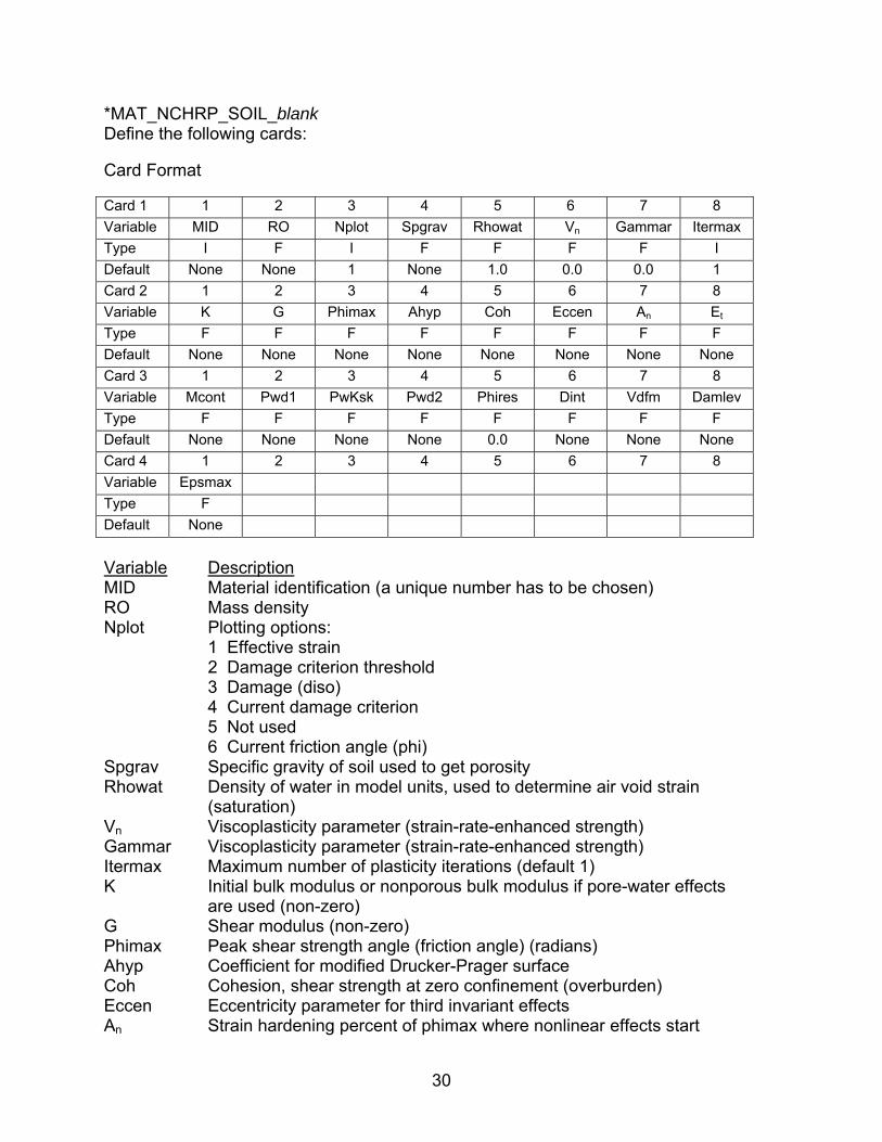
*MAT_NCHRP_SOIL_blank Define the following cards: Card Format Card 1 1 2 3 4 5 6 7 8 Variable MID RO Nplot Spgrav Rhowat Vn Gammar Itermax Type I F I F F F F I Default None None 1 None 1.0 0.0 0.0 1 Card 2 1 2 3 4 5 6 7 8 Variable K G Phimax Ahyp Coh Eccen An Et Type F F F F F F F F Default None None None None None None None None Card 3 1 2 3 4 5 6 7 8 Variable Mcont Pwd1 PwKsk Pwd2 Phires Dint Vdfm Damlev Type F F F F F F F F Default None None None None 0.0 None None None Card 4 1 2 3 4 5 6 7 8 Variable Epsmax Type F Default None

Variable Description MID Material identification (a unique number has to be chosen) RO Mass density Nplot Plotting options:

1 Effective strain 2 Damage criterion threshold 3 Damage (diso) 4 Current damage criterion 5 Not used 6 Current friction angle (phi) Spgrav Specific gravity of soil used to get porosity Rhowat Density of water in model units, used to determine air void strain

(saturation) Vn Viscoplasticity parameter (strain-rate-enhanced strength) Gammar Viscoplasticity parameter (strain-rate-enhanced strength) Itermax Maximum number of plasticity iterations (default 1) K Initial bulk modulus or nonporous bulk modulus if pore-water effects

are used (non-zero) G Shear modulus (non-zero) Phimax Peak shear strength angle (friction angle) (radians) Ahyp Coefficient for modified Drucker-Prager surface Coh Cohesion, shear strength at zero confinement (overburden) Eccen Eccentricity parameter for third invariant effects An Strain hardening percent of phimax where nonlinear effects start

31

Et Strain hardening amount of nonlinear effects Mcont Moisture content of soil (determines amount of air voids) (0-1.00) Pwd1 Parameter for pore-water effects on bulk modulus PwKsk Skeleton bulk modulus, pore-water parameter, set to zero to

eliminate effects Pwd2 Parameter for pore-water effects on effective pressure (confinement) Phires Minimum internal friction angle (radians) (residual shear strength) Dint Volumetric strain at initial damage threshold ( 0ξ ) Vdfm Void formation energy (like fracture energy) Damlev Level of damage that will cause element deletion (0.0-1.0) Epsmax Maximum principal failure strain THEORY MANUAL MAT_FHWA_SOIL A brief discussion of the FHWA soil model is given. The elastic properties of the soil are isotropic. The implementation of the modified Mohr-Coulomb plasticity surface is based on the work of Abbo and Sloan.(9) The model is extended to include excess pore-water effects, strain softening, kinematic hardening, strain-rate effects, and element deletion. The modified yield surface is a hyperbola fitted to the Mohr-Coulomb surface. At the crossing of the pressure axis (zero shear strength), the modified surface is a smooth surface and it is perpendicular to the pressure axis. The yield surface is given as:

(20) where: P = pressure ϕ = internal friction angle

)(θK = function of the angle in deviatoric plane

2J = square root of the second invariant of the stress deviator

c = amount of cohesion, 23

2

3

2

333cos

J

J=θ

3J = third invariant of the stress deviator ahyp = parameter for determining how close to the standard Mohr-Coulomb yield surface the modified surface is fitted

0cos2sin22)(2sin =−++−= ϕϕθϕ cahypKJPF

32

If ahyp is input as zero, the standard Mohr-Coulomb surface is recovered. The input parameter ahyp should be set close to zero, based on numerical considerations, but always less than ϕcotc . It is best not to set the cohesion, c, to very small values since this causes excessive iterations in the plasticity routines. To generalize the shape in the deviatoric plane, the standard Mohr-Coulomb )(θK function was changed to a function used by Klisinski:(10)

21

2222

222

]45cos)1(4)[12(cos)1(2

)12(cos)1(4)(eeeee

eeK−+−−+−

−+−=

θθ

θθ (21)

where:

23

2

3

2

333cos

J

J=θ

3J = third invariant of the stress deviator e = material parameter describing the ratio of triaxial extension strength to triaxial compression strength If e is set to 1, then a circular cone surface is formed. If e is set to 0.55, then a triangular surface is formed. )(θK is defined for 0.15.0 ≤< e . To simulate nonlinear strain hardening behavior, the friction angle ϕ is increased as a function of the effective plastic strain:

plaseffn

initt A

E εφφφ

φ ∆−

−=∆ )1(max

(22)

where:

plaseffε = effective plastic strain

nA = fraction of the peak strength internal friction angle where nonlinear behavior begins, 10 ≤< nA The input parameter tE determines the rate of the nonlinear hardening. If there is no strain hardening, then ϕϕϕ == initmax . To simulate the effects of moisture and air voids, including excess pore-water pressure, both the elastic and plastic behaviors can be modified. The bulk modulus is:

33

curi

i

nDKK

K11 +

= (23)

where:

iK = nonporous bulk modulus

curn = current porosity = )](,0[ vwMax ε−

w = volumetric strain corresponding to the volume of air voids = )1( Sn −

vε = total volumetric strain

1D = material constant controlling the stiffness before the air voids are collapsed

n = porosity of the soil = e

e+1

e = void ratio = 1)1(

−+

ρ

ργ cwsp m

S = degree of saturation = )1( cw

cmn

m+ρ

ρ

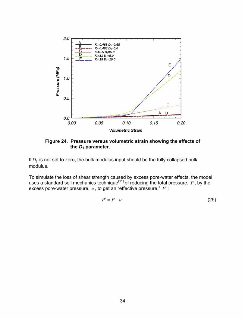
wcsp m,γρ, ρ, = soil density, specific gravity, moisture content, and water density. Figure 24 shows the effect of the D1 parameter on the pressure-volumetric strain relationship (bulk modulus). The bulk modulus will always be a monotonically increasing value, that is:

⎪⎩

⎪⎨⎧

≤

>+=

+

++

vjjvj

vjjvcuri

i

j

ifK

ifnDK

KK

εε

εε

1

111 1 (24)

Note that the model is following the standard practice of assuming that compressive stresses and strains are positive. If the input parameter 1D is zero, then the standard linear elastic bulk modulus behavior is used.

34

Figure 24. Pressure versus volumetric strain showing the effects of the D1 parameter.

If 1D is not set to zero, the bulk modulus input should be the fully collapsed bulk modulus. To simulate the loss of shear strength caused by excess pore-water effects, the model uses a standard soil mechanics technique(11) of reducing the total pressure, P , by the excess pore-water pressure, u , to get an “effective pressure,” P′ :

uPP −=′ (25)

A B

A B

C

C

D

D

E E

Ki=0.468 D1=0.68 Ki=0.468 D1=5.0 Ki=2.5 D1=5.0 Ki=11 D1=5.0 Ki=15 D1=10.0

Volumetric Strain

Pres

sure

(MPa

)

35

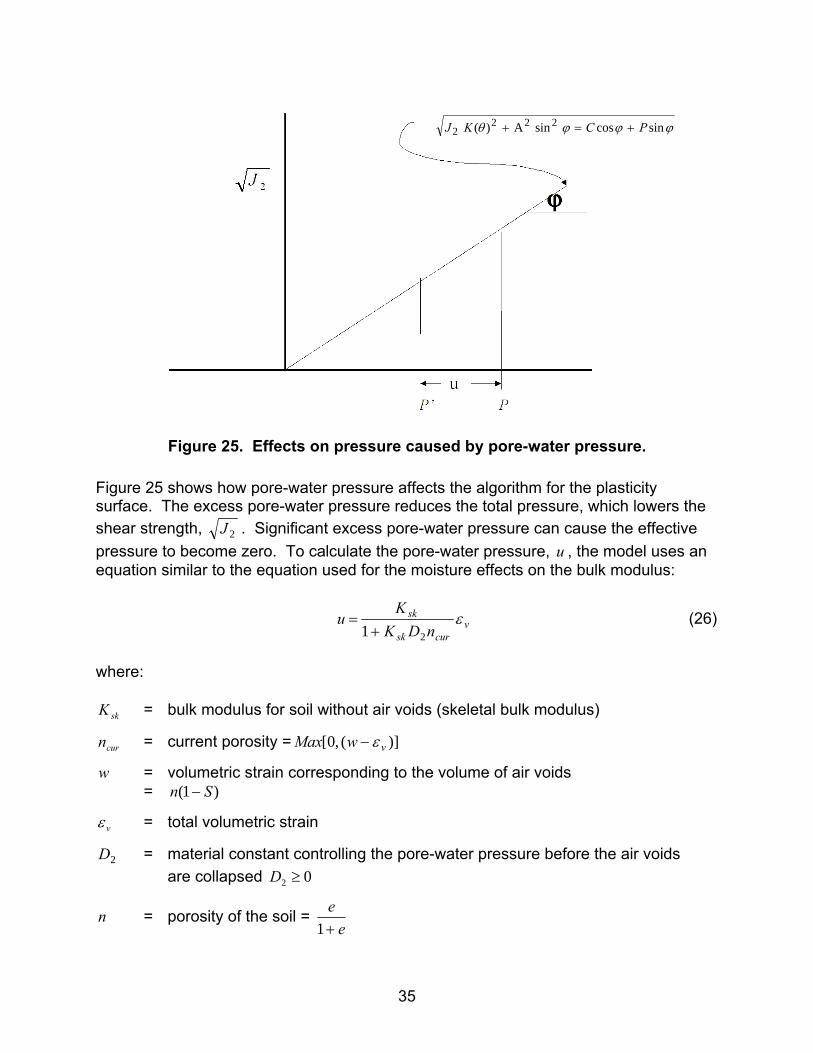
Figure 25. Effects on pressure caused by pore-water pressure. Figure 25 shows how pore-water pressure affects the algorithm for the plasticity surface. The excess pore-water pressure reduces the total pressure, which lowers the shear strength, 2J . Significant excess pore-water pressure can cause the effective pressure to become zero. To calculate the pore-water pressure, u , the model uses an equation similar to the equation used for the moisture effects on the bulk modulus:

vcursk

sk

nDKK

u ε21 +

= (26)

where:

skK = bulk modulus for soil without air voids (skeletal bulk modulus)

curn = current porosity = )](,0[ vwMax ε−

w = volumetric strain corresponding to the volume of air voids = )1( Sn −

vε = total volumetric strain

2D = material constant controlling the pore-water pressure before the air voids are collapsed 02 ≥D

n = porosity of the soil = e

e+1

ϕϕϕθ sincossinA)( 2222 PCKJ +=+

36

e = void ratio = 1)1(

−+

ργ csp m

S = degree of saturation = )1( c

c

mnm+

ρ

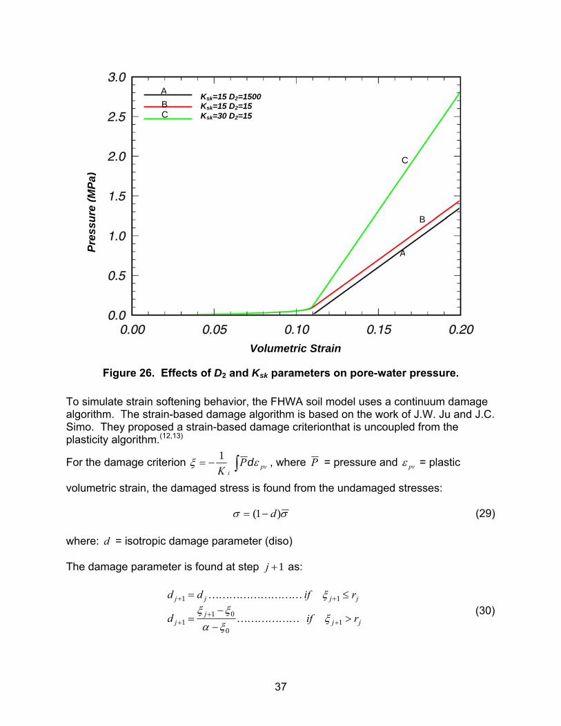
csp m,, γρ = soil density, specific gravity, and moisture content, respectively The increment pore-water pressure is zero if the incremental mean strain is negative (tensile). Figure 26 is a plot of the pore pressure versus volumetric strain for different parameter values. With the D2 parameter set relatively high compared to Ksk, there is no pore pressure until the volumetric strain is greater than the strains associated with the air voids. However, as D2 is lowered, the pore pressure starts to increase before the air voids are totally collapsed. The Ksk parameter affects the slope of the post-void collapse pressure-volumetric strain behavior. The parameter D2 is found from Skempton pore-water pressure parameter B, where B is defined as:(7)

KKn

Bsk+

=1

1 (27)

)]1([1

2 SnKBBD

sk −−

=∴ (28)

37

Figure 26. Effects of D2 and Ksk parameters on pore-water pressure.

To simulate strain softening behavior, the FHWA soil model uses a continuum damage algorithm. The strain-based damage algorithm is based on the work of J.W. Ju and J.C. Simo. They proposed a strain-based damage criterionthat is uncoupled from the plasticity algorithm.(12,13)

For the damage criterion ∫−= pvi

PK

εξ d1 , where P = pressure and pvε = plastic

volumetric strain, the damaged stress is found from the undamaged stresses:

σσ )1( d−= (29) where: d = isotropic damage parameter (diso) The damage parameter is found at step 1+j as:

jjj

j

jjjj

rifd

rifdd

>−−

=

≤=

++

+

++

10

011

11

ξξαξξ

ξ

KKKKKK

KKKKKKKKK

(30)

A

A

B

B

C

C

Ksk=15 D2=1500 Ksk=15 D2=15 Ksk=30 D2=15

Pres

sure

(MPa

)

Volumetric Strain

38

where: 1+jr = damage threshold surface

),max( 11 ++ = jjj rr ξ

00 r=ξ (Dint)

The mesh-sensitivity parameter, α , is described below. Typically, the damage, d, varies from 0 to a maximum of 1. However, some soils can have a residual strength that is pressure-dependent. The residual strength is represented by resϕ , the minimum internal friction angle. The maximum damage allowed is related to the internal friction angle of residual strength by:

ϕϕϕ

sinsinsin

maxresd

−= (31)

If 0>resϕ , then maxd , the maximum damage, will not reach 1 and the soil will have residual strength. When material models include strain softening, special techniques must be used to prevent mesh sensitivity. Mesh sensitivity is the tendency of the finite element model/analysis to produce significantly different results as the element size is reduced. Mesh sensitivity occurs because the softening in the model is concentrated in one element. As the element size is reduced, the failure becomes localized in smaller volumes, which causes less energy to be dissipated by the softening. This can lead to instabilities or, at least, mesh-sensitive behavior. To eliminate or reduce the effects of strain softening mesh sensitivity, the softening parameter, α (the strain at full damage), must be modified as the element size changes. The FHWA soil model uses an input parameter, “void formation,” fG , that is like the fracture energy material property for metals. The void formation parameter is the area under the softening region of the pressure-volumetric strain curve times the cube root of the element volume, 3

1V :

2)(

d3

1

0

31 0peak

vVP

PVG fξα

εαξ

−== ∫ (32)

with 0ξ as the volumetric strain at peak pressure (strain at initial damage (Dint)). Then,

α can be found as a function of the volume of the elementV :

39

03

10

f2ξ

ξα +=

VK

G (33)

If fG is made very small relative to 3

1

0VKξ , then the softening behavior will be brittle. Strain-rate-enhanced strength is simulated by a two-parameter Devaut-Lions viscoplastic update algorithm developed by Y. Murray.(15) This algorithm interpolates between the elastic trial stress (beyond the plasticity surface) and the inviscid stress. The inviscid stresses (σ ) are on the plasticity surface trialvp σςσςσ +−= )1( , with

ηης+∆

=t

and vnvnr /)1()( −=εγη&

.

As ζ becomes 1, then the viscoplastic stress becomes the elastic trial stress. Setting the input value 0=rγ (gamma) eliminates any strain-rate-enhanced strength effects. The model allows element deletion if needed. As the strain softening (damage) increases, the effective stiffness of the element can become very small, causing severe element distortion and “hourglassing.” The element can be “deleted” to remedy this behavior. There are two input parameters that affect the point of element deletion. Damlev is the damage threshold where element deletion will be considered. Epsmax is the maximum principal strain where the element will be deleted. Both d ≥ Damlev and

>maxprε Epsmax are required for element deletion to occur. If Damlev is set to zero, there is no element deletion. Care must be taken when employing element deletion to ensure that the internal forces are very small (element stiffness is zero) or significant errors may be introduced into the analysis. MAT_FHWA_SOIL_NEBRASKA This option gives the soil parameters that were used to validate the material model with experiments performed at the University of Nebraska at Lincoln. The units of these default inputs are milliseconds, kilograms, and millimeters. There are no required input parameters except for material ID (MID). If different units are desired, the appropriate unit conversion factors can be input. DISCUSSION OF SOIL MODEL USE

Material models for geomaterials (soils, concrete, rock, etc.) tend to be complex. The determination of the input parameters for the models is complicated. In addition, modeling different loading conditions and accurate simulation of boundary conditions add to the complexity involved in using these material models. There are two methods that are typically used to determine the material input variables for soils. The most accurate method is to perform laboratory tests that include both triaxial compression and uniaxial strain tests. These tests can be used to determine the

40

elastic moduli, yield surface parameters, and softening parameters. Typically, these tests use drained soil conditions. Laboratory tests with undrained soil conditions can be used to determine the pore-water effects. A second method is to use full-scale testing of the specific application (e.g., a bogie impacting a steel post) to fit the parameters in a trial-and-error method. This method requires more time by the analyst. Since the soil model is nonlinear, there may not be a set of unique input parameters that can be determined. Compaction of the soil is typically used to remove some of the air voids that exist in disturbed soils. However, the density, pore-water effects, stiffness, and strength are also changed upon compacting the soil. To simulate compaction in highway safety applications where the soil is exposed, we recommend that the values for the soil density, pore-water effects, stiffness, and strength be modified. Applying pressure to the ground surface to account for the effects of compaction is a less accurate method that will incorrectly simulate how the soil is deformed at the surface. In full-scale testing or applications, the soil typically extends to infinity. Analyses typically do not extend to infinity, so some type of boundary condition must be applied to the exterior surfaces of a soil analysis model (except for soil surfaces exposed to atmospheric pressure). Standard boundaries reflect dynamic disturbances (stress waves), which does not happen in the real applications. Such reflections can cause serious contamination of the analysis results. Exterior boundaries for analyses involving soil need a nonreflecting boundary. A partial nonreflecting boundary exists in LS-DYNA. This boundary is an impedance-matching boundary, which is only good for high-frequency (highly transient) behavior. At this time, there is no nonreflecting boundary that matches both low- (quasi-static) and high- (highly transient) frequency behaviors. Also, only linear behavior is assumed. Thus, to use the current nonreflecting boundary, the material near the boundaries must only behave linearly. Also, the nonreflecting boundary should only experience high-frequency behavior.

41

CHAPTER 3. EXAMPLES MANUAL

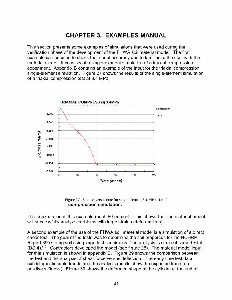
This section presents some examples of simulations that were used during the verification phase of the development of the FHWA soil material model. The first example can be used to check the model accuracy and to familiarize the user with the material model. It consists of a single-element simulation of a triaxial compression experiment. Appendix B contains an example of the input for the triaxial compression single-element simulation. Figure 27 shows the results of the single-element simulation of a triaxial compression test at 3.4 MPa.

Figure 27. Z-stress versus time for single-element 3.4-MPa triaxial compression simulation.

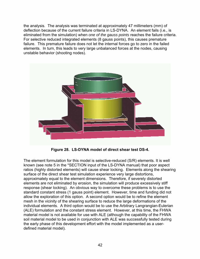
The peak strains in this example reach 80 percent. This shows that the material model will successfully analyze problems with large strains (deformations). A second example of the use of the FHWA soil material model is a simulation of a direct shear test. The goal of the tests was to determine the soil properties for the NCHRP Report 350 strong soil using large test specimens. The analysis is of direct shear test 4 (DS-4).(16) Contractors developed the model (see figure 28). The material model input for this simulation is shown in appendix B. Figure 29 shows the comparison between the test and the analysis of shear force versus deflection. The early time test data exhibit questionable trends and the analysis results show the expected trend (i.e., positive stiffness). Figure 30 shows the deformed shape of the cylinder at the end of

TRIAXIAL COMPRESS @ 3.4MPa

-0.002

-0.004

-0.006

-0.008

-0.01

-0.012

-0.014

-0.016

Z-St

ress

Time (msec)

Z-St

ress

(MPa

)

42

the analysis. The analysis was terminated at approximately 47 millimeters (mm) of deflection because of the current failure criteria in LS-DYNA. An element fails (i.e., is eliminated from the simulation) when one of the gauss points reaches the failure criteria. For selective reduced integrated elements (8 gauss points), this causes premature failure. This premature failure does not let the internal forces go to zero in the failed elements. In turn, this leads to very large unbalanced forces at the nodes, causing unstable behavior (shooting nodes).

Figure 28. LS-DYNA model of direct shear test DS-4.

The element formulation for this model is selective-reduced (S/R) elements. It is well known (see note 5 in the *SECTION input of the LS-DYNA manual) that poor aspect ratios (highly distorted elements) will cause shear locking. Elements along the shearing surface of the direct shear test simulation experience very large distortions, approximately equal to the element dimensions. Therefore, if severely distorted elements are not eliminated by erosion, the simulation will produce excessively stiff response (shear locking). An obvious way to overcome these problems is to use the standard constant stress (1 gauss point) element. However, time and funding did not allow the exploration of this option. A second option would be to refine the element mesh in the vicinity of the shearing surface to reduce the large deformations of the individual elements. A third option would be to use the Arbitrary Langrangian-Eulerian (ALE) formulation and the constant stress element. However, at this time, the FHWA material model is not available for use with ALE (although the capability of the FHWA soil material model to be used in conjunction with ALE was successfully tested during the early phase of this development effort with the model implemented as a user-defined material model).

43

As shown in figure 30, there are surfaces of the soil, which at the time of the analysis, are in contact with the metal or air. Also, the interface between the two cylinder halves has become a noncontinuous surface (i.e., a slide surface). This behavior cannot be accurately modeled by the continuum mechanics material model; it must be modeled by slide surfaces.

0

10

20

30

40

50

60

-1.00E+01 0.00E+00 1.00E+01 2.00E+01 3.00E+01 4.00E+01 5.00E+01 6.00E+01 7.00E+01 8.00E+01

Deflection (mm)

shea

r for

ce k

Pa

LSDYNA test data ds-4

Figure 29. Shear stress versus deflection comparison for DS-4.

Figure 30. Analysis results for DS-4 deformation.

LS-DYNA A

A

B

B

A LS-DYNA B Test Data DS-4

Shee

r For

ce (k

Pa)

44

To further investigate the behavior of the soil model in shear stress, a model used in the development of the model was run with both 1 gauss point (elform = 1) and 8 gauss point (elform = 2) elements. Figure 31 shows the model, which consists of two materials (the material on the left is the FHWA soil material and the material on the right is a relatively stiff elastic material). A velocity boundary condition is applied to the free soil surface in the vertical position.

Figure 31. Simple two-material shear model.

The input parameters for the soil material were from the direct shear analysis. Figure 32 shows the deformed shape of the 1 gauss point element analysis at 1.75 milliseconds (ms), and figure 33 shows the deformed shape of the 8 gauss point element analysis at 1.75 ms. The analyses were stopped just before the 8 gauss point element becomes unstable because of the failure criteria error in the 8 gauss point element (outside the material subroutine). Figure 34 shows the x-y shear stress in element 115 (shown in the previous figures). Since the soil material has a low cohesion (shear strength at zero normal force) of 6.2 x 10-6 gigapascals (GPa) (6.2 kilopascals (KPa)), the x-y shear stress should not get very large. The 8 gauss point element shows an immediate increase in the x-y shear stress to more than 0.03 GPa (30 MPa); this type of behavior is known as “shear locking.” It is caused by the formulation of the 8 gauss point element outside of the material routine. As mentioned previously, this inaccurate behavior is mentioned in the

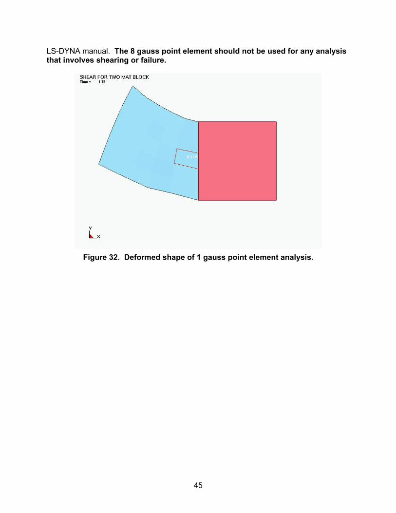
45

LS-DYNA manual. The 8 gauss point element should not be used for any analysis that involves shearing or failure.

Figure 32. Deformed shape of 1 gauss point element analysis.

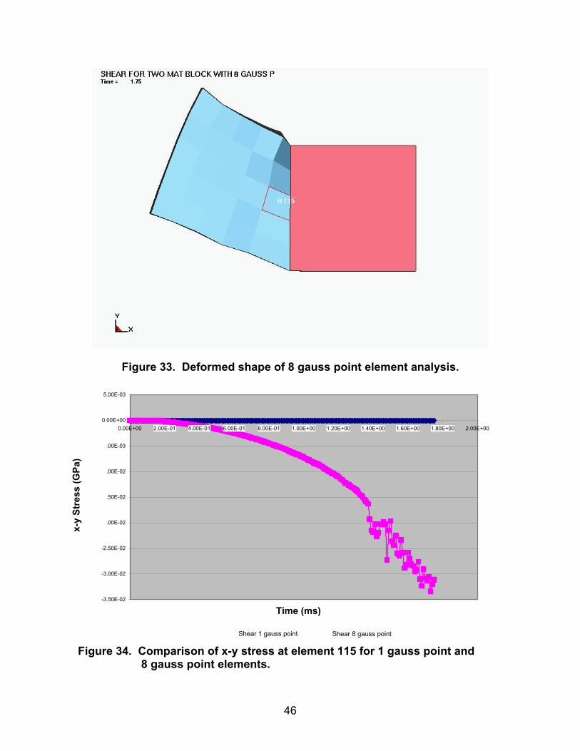
46

Figure 33. Deformed shape of 8 gauss point element analysis.

-3.50E-02

-3.00E-02

-2.50E-02

-2.00E-02

-1.50E-02

-1.00E-02

-5.00E-03

0.00E+00

5.00E-03

0.00E+00 2.00E-01 4.00E-01 6.00E-01 8.00E-01 1.00E+00 1.20E+00 1.40E+00 1.60E+00 1.80E+00 2.00E+00

Time (msecs)

XY S

tres

s (G

pa)

shear 1 gauss point Shear 8 gauss point

Figure 34. Comparison of x-y stress at element 115 for 1 gauss point and 8 gauss point elements.

x-y

Stre

ss (G

Pa)

Time (ms)

Shear 1 gauss point Shear 8 gauss point

47

The material properties used in the simulations/examples described above were not determined from actual material property test data, but were found by trial and error. Obviously, actual material property data would probably lead to more confident results.

49

CHAPTER 4. SUMMARY This report presents the theory manual, user’s manual, and typical examples for the FHWA soil material model implemented into LS-DYNA. This model was developed for use in roadside safety applications. The model is a modified Drucker-Prager plasticity model. In addition to the plasticity model, the FHWA soil material model includes pre-peak hardening, post-peak strain softening (damage), strain-rate effects (strength enhancement), pore-water effects (moisture effects), and erosion capability. These enhancements to the standard soil material models were made to increase the accuracy, robustness, and ease of use for roadside safety applications. The theory manual gives a detailed description of the model, including the justification, equations, and methods of implementation of the equations. Developers should be able to use the theory manual to make modifications to, or maintain, the FHWA soil material model. Appendix A presents the details of the determination of the plasticity gradients. The user’s manual is a contractor’s user’s manual for the FHWA soil material model. Also included is a table that shows the correspondence between the symbols used in the theory manual and the input variables in the user’s manual. A brief discussion of the use of the model in roadside safety applications is also included in this section. Finally, typical examples are presented. These examples should help the user prepare the input and check out the model for their versions of LS-DYNA. The direct shear test simulation was stopped at approximately 46 ms because of shear locking and premature erosion (deletion) of the selectively reduced integration (8 gauss integration point) elements. The problem of shear locking is well known for this type of element when the element is subjected to large distortions. Premature erosion of this element type is a deficiency of the current version of LS-DYNA (version 970 Beta) and is not ascribable to improper functioning of the FHWA soil material model. The use of ALE with constant stress elements (1 gauss integration point) may produce results with greater simulation times. Presently, the FHWA soil material model has been shown to be accurate for small soil samples at all levels of deformation and for large simulations that involve small to intermediate deformations. This restriction is caused by limitations in the current version of LS-DYNA. Additional work is recommended to provide a more robust FHWA soil material model. This work includes investigation of the use of ALE for simulations involving large distortions, investigation/development of nonreflecting boundaries, and further simulations investigating moisture and strain-rate effects. Additional testing would be advantageous for the determination of accurate material properties (soil material model input).

51

APPENDIX A. DETERMINATION OF PLASTICITY GRADIENTS

In the following, the gradient of the yield surface in stress space is determined. The yield function is:

ϕϕθϕ cosc2sin2a2)(2sin −++−= KJPF (34)

where:

21

2222

222

]45cos)1(4)[12(cos)1(2

)12(cos)1(4)(eeeee

eeK−+−−+−

−+−=

θθ

θθ

23

2

3

2

333cos

J

J=θ

3J = third invariant of the stress deviator

e = material parameter describing the ratio of triaxial extension strength to triaxial compression strength

We need to find σ∂

∂F . A convenient method is:

σσσσ

33

221

JC

JCpCF ∂

+∂

∂+

∂=

∂∂ (35)

where:

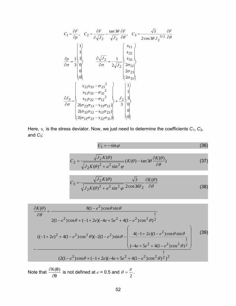
52

⎪⎪⎪⎪

⎭

⎪⎪⎪⎪

⎬

⎫

⎪⎪⎪⎪

⎩

⎪⎪⎪⎪

⎨

⎧

+

⎪⎪⎪⎪

⎭

⎪⎪⎪⎪

⎬

⎫

⎪⎪⎪⎪

⎩

⎪⎪⎪⎪

⎨

⎧

−−−−−−

=∂∂

⎪⎪⎪⎪

⎭

⎪⎪⎪⎪

⎬

⎫

⎪⎪⎪⎪

⎩

⎪⎪⎪⎪

⎨

⎧

=∂

∂

⎪⎪⎪⎪

⎭

⎪⎪⎪⎪

⎬

⎫

⎪⎪⎪⎪

⎩

⎪⎪⎪⎪

⎨

⎧

=∂∂

∂∂

=∂∂

−∂

∂=

∂∂

=

000111

3

)s(2)s(2)s(2

ssssss

222sss

21

000111

31

3cos2

3,3tan,

2

31222312

23111231

12331323

2122211

2313311

2233322

3

31

23

12

33

22

11

2

2

2/32

322

21

JJ

J

Jp

F

JCF

JJFC

pFC

σσσσσσσσσ

σσσ

σ

σσσσσ

θθθθ

Here, is is the stress deviator. Now, we just need to determine the coefficients C1, C2, and C3:

ϕsin1 −=C (36)

))(3tan)((sin)(

)(222

2

22 θ

θθθϕθ

θ∂

∂−

+=

KKaKJ

KJC (37)

θθ

θϕθ

θ∂

∂

+=

)(3cos23

sin)(

)(

22222

23

KJaKJ

KJC

(38)

221

2222

21

222

22222

21

2222

2

))cos)1(454)(21(cos)1(2(

)cos)1(454(

sincos)1)(21(4sin)1(2)(cos)1(4)21((

)cos)1(454)(21(cos)1(2

sincos)1(8)(

θθ

θ

θθθθ

θθ

θθθθ

eeeee

eee

eeeee

eeeee

eK

−++−+−+−

⎟⎟⎟⎟

⎠

⎞

⎜⎜⎜⎜

⎝

⎛

−++−

−+−−−−−++−

−

−++−+−+−

−=

∂∂

(39)

Note that θθ

∂∂ )(K is not defined at e = 0.5 and

2πθ = .

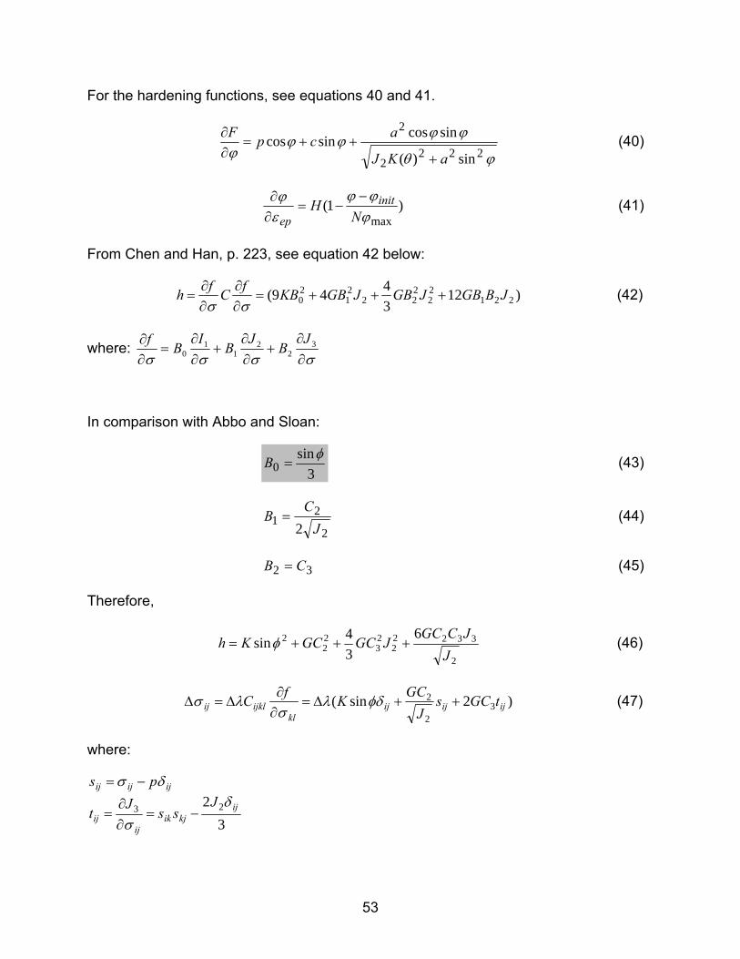
53

For the hardening functions, see equations 40 and 41.

ϕθ

ϕϕϕϕϕ 222

2

2

sin)(

sincossincosaKJ

acpF

+++=

∂∂ (40)

)1(maxϕϕϕ

εϕ

NH init

ep

−−=

∂∂ (41)

From Chen and Han, p. 223, see equation 42 below:

)123449( 221

22

222

21

20 JBGBJGBJGBKBfCfh +++=

∂∂

∂∂

=σσ

(42)

where: σσσσ ∂

∂+

∂∂

+∂∂

=∂∂ 3

22

11

0J

BJBIBf

In comparison with Abbo and Sloan:

3sin

0φ

=B (43)

2

21 2 J

CB = (44)

32 CB = (45)

Therefore,

2

33222

23

22

2 634sin

JJCGC

JGCGCKh +++= φ (46)

)2sin( 32

2ijijij

klijklij tGCs

JGCKfC ++∆=

∂∂

∆=∆ φδλσ

λσ (47)

where:

32 23 ij

kjikij

ij

ijijij

JssJt

psδ

σ

δσ

−=∂∂

=

−=

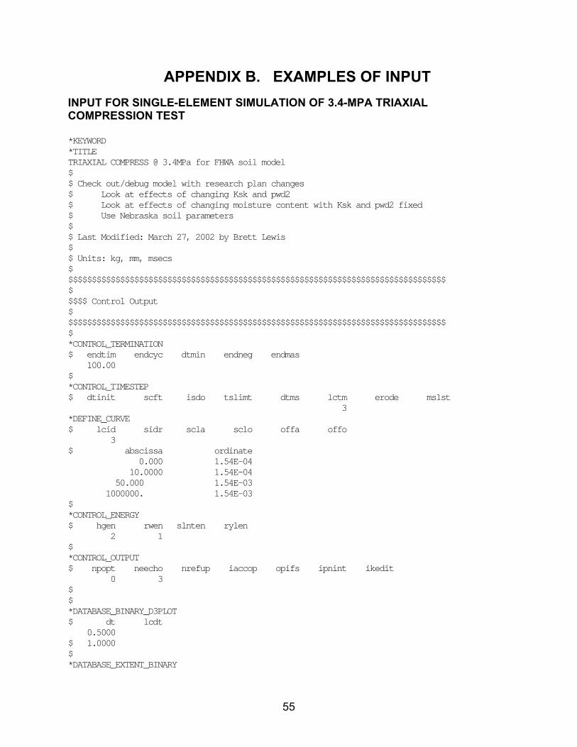
55

APPENDIX B. EXAMPLES OF INPUT INPUT FOR SINGLE-ELEMENT SIMULATION OF 3.4-MPA TRIAXIAL COMPRESSION TEST *KEYWORD *TITLE TRIAXIAL COMPRESS @ 3.4MPa for FHWA soil model $ $ Check out/debug model with research plan changes $ Look at effects of changing Ksk and pwd2 $ Look at effects of changing moisture content with Ksk and pwd2 fixed $ Use Nebraska soil parameters $ $ Last Modified: March 27, 2002 by Brett Lewis $ $ Units: kg, mm, msecs $ $$$$$$$$$$$$$$$$$$$$$$$$$$$$$$$$$$$$$$$$$$$$$$$$$$$$$$$$$$$$$$$$$$$$$$$$$$$$$$$$ $ $$$$ Control Output $ $$$$$$$$$$$$$$$$$$$$$$$$$$$$$$$$$$$$$$$$$$$$$$$$$$$$$$$$$$$$$$$$$$$$$$$$$$$$$$$$ $ *CONTROL_TERMINATION $ endtim endcyc dtmin endneg endmas 100.00 $ *CONTROL_TIMESTEP $ dtinit scft isdo tslimt dtms lctm erode ms1st 3 *DEFINE_CURVE $ lcid sidr scla sclo offa offo 3 $ abscissa ordinate 0.000 1.54E-04 10.0000 1.54E-04 50.000 1.54E-03 1000000. 1.54E-03 $ *CONTROL_ENERGY $ hgen rwen slnten rylen 2 1 $ *CONTROL_OUTPUT $ npopt neecho nrefup iaccop opifs ipnint ikedit 0 3 $ $ *DATABASE_BINARY_D3PLOT $ dt lcdt 0.5000 $ 1.0000 $ *DATABASE_EXTENT_BINARY

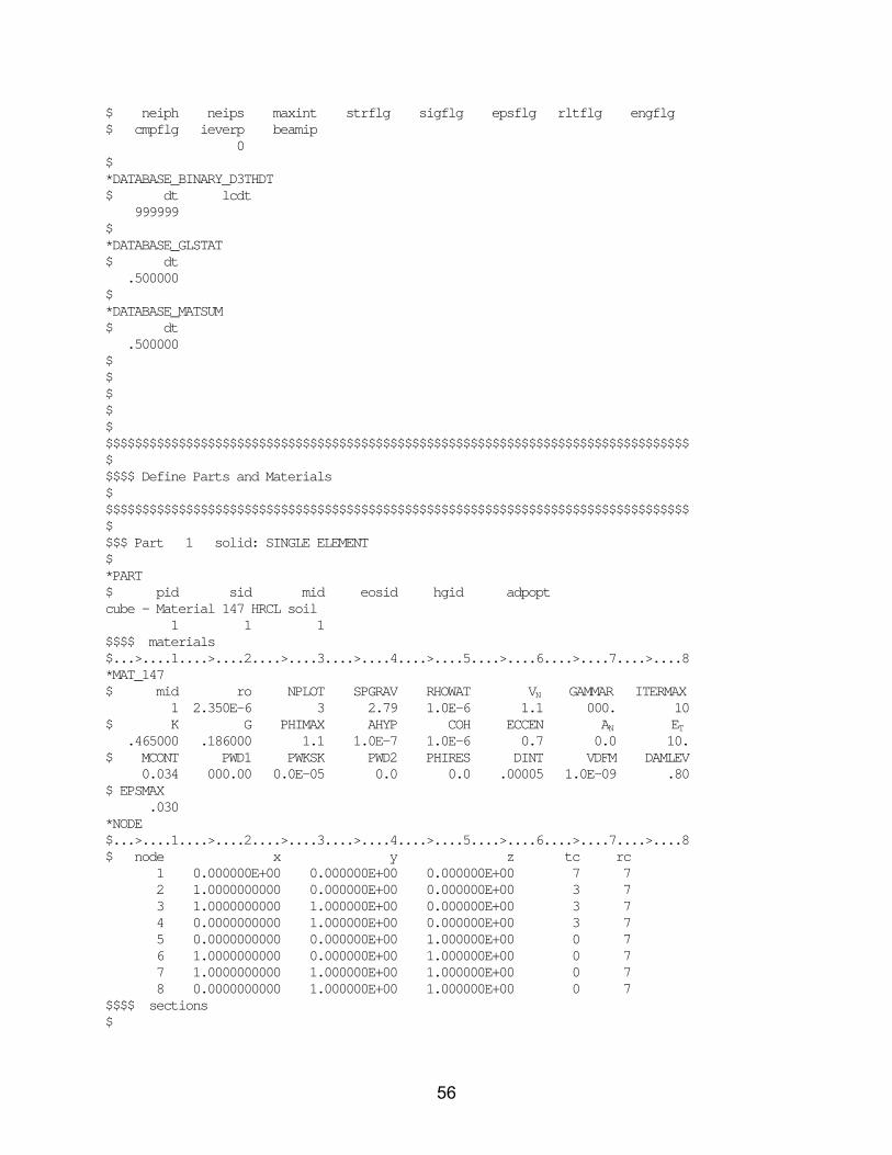
56

$ neiph neips maxint strflg sigflg epsflg rltflg engflg $ cmpflg ieverp beamip 0 $ *DATABASE_BINARY_D3THDT $ dt lcdt 999999 $ *DATABASE_GLSTAT $ dt .500000 $ *DATABASE_MATSUM $ dt .500000 $ $ $ $ $ $$$$$$$$$$$$$$$$$$$$$$$$$$$$$$$$$$$$$$$$$$$$$$$$$$$$$$$$$$$$$$$$$$$$$$$$$$$$$$$$ $ $$$$ Define Parts and Materials $ $$$$$$$$$$$$$$$$$$$$$$$$$$$$$$$$$$$$$$$$$$$$$$$$$$$$$$$$$$$$$$$$$$$$$$$$$$$$$$$$ $ $$$ Part 1 solid: SINGLE ELEMENT $ *PART $ pid sid mid eosid hgid adpopt cube - Material 147 HRCL soil 1 1 1 $$$$ materials $...>....1....>....2....>....3....>....4....>....5....>....6....>....7....>....8 *MAT_147 $ mid ro NPLOT SPGRAV RHOWAT VN GAMMAR ITERMAX 1 2.350E-6 3 2.79 1.0E-6 1.1 000. 10 $ K G PHIMAX AHYP COH ECCEN AN ET .465000 .186000 1.1 1.0E-7 1.0E-6 0.7 0.0 10. $ MCONT PWD1 PWKSK PWD2 PHIRES DINT VDFM DAMLEV 0.034 000.00 0.0E-05 0.0 0.0 .00005 1.0E-09 .80 $ EPSMAX .030 *NODE $...>....1....>....2....>....3....>....4....>....5....>....6....>....7....>....8 $ node x y z tc rc 1 0.000000E+00 0.000000E+00 0.000000E+00 7 7 2 1.0000000000 0.000000E+00 0.000000E+00 3 7 3 1.0000000000 1.000000E+00 0.000000E+00 3 7 4 0.0000000000 1.000000E+00 0.000000E+00 3 7 5 0.0000000000 0.000000E+00 1.000000E+00 0 7 6 1.0000000000 0.000000E+00 1.000000E+00 0 7 7 1.0000000000 1.000000E+00 1.000000E+00 0 7 8 0.0000000000 1.000000E+00 1.000000E+00 0 7 $$$$ sections $

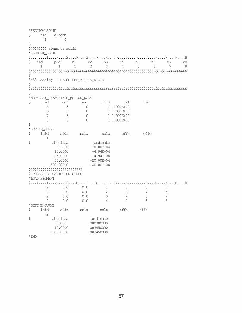
57

*SECTION_SOLID $ sid elform 1 0 $ $$$$$$$$$ elements solid *ELEMENT_SOLID $...>....1....>....2....>....3....>....4....>....5....>....6....>....7....>....8 $ eid pid n1 n2 n3 n4 n5 n6 n7 n8 1 1 1 2 3 4 5 6 7 8 $$$$$$$$$$$$$$$$$$$$$$$$$$$$$$$$$$$$$$$$$$$$$$$$$$$$$$$$$$$$$$$$$$$$$$$$$$$$$$$$ $ $$$$ Loading - PRESCRIBED_MOTION_RIGID $ $$$$$$$$$$$$$$$$$$$$$$$$$$$$$$$$$$$$$$$$$$$$$$$$$$$$$$$$$$$$$$$$$$$$$$$$$$$$$$$$ $ *BOUNDARY_PRESCRIBED_MOTION_NODE $ nid dof vad lcid sf vid 5 3 0 1 1.000E+00 6 3 0 1 1.000E+00 7 3 0 1 1.000E+00 8 3 0 1 1.000E+00 $ *DEFINE_CURVE $ lcid sidr scla sclo offa offo 1 $ abscissa ordinate 0.000 -0.00E-04 10.0000 -4.94E-04 25.0000 -4.94E-04 50.0000 -20.00E-04 500.00000 -40.00E-04 $$$$$$$$$$$$$$$$$$$$$$$$$$$ $ PRESSURE LOADING ON SIDES *LOAD_SEGMENT $...>....1....>....2....>....3....>....4....>....5....>....6....>....7....>....8 2 0.0 0.0 1 2 6 5 2 0.0 0.0 2 3 7 6 2 0.0 0.0 3 4 8 7 2 0.0 0.0 4 1 5 8 *DEFINE_CURVE $ lcid sidr scla sclo offa offo 2 $ abscissa ordinate 0.000 .000000000 10.0000 .003450000 500.00000 .003450000 *END

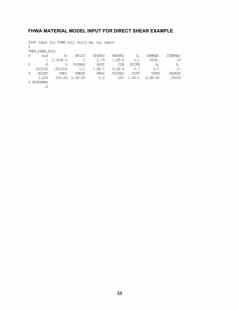
58

FHWA MATERIAL MODEL INPUT FOR DIRECT SHEAR EXAMPLE

$$$$ Input for FHWA soil Units mm, kg, msecs $ *MAT_FHWA_SOIL $ mid ro NPLOT SPGRAV RHOWAT VN GAMMAR ITERMAX 1 2.350E-6 3 2.79 1.0E-6 1.1 0000. 10 $ K G PHIMAX AHYP COH ECCEN AN ET .003250 .001300 1.1 1.0E-7 6.2E-6 0.7 0.0 0. $ MCONT PWD1 PWKSK PWD2 PHIRES DINT VDFM DAMLEV 0.034 000.00 0.0E-05 0.0 .001 1.0E-5 6.0E-08 .99000 $ EPSPRMAX .8

59

REFERENCES 1. Hallquist, J.O., LS-DYNA Keyword User’s Manual, Version 960, Livermore

Software Technology Corporation, Livermore, CA, March 2001.

2. Reid, J.D., B.A. Coon, B.A. Lewis, S.H. Sutherland, and Y.D. Murray, Evaluation of LS-DYNA Soil Material Model 147, Report No. FHWA-HRT-04-094, Federal Highway Administration, November 2004.

3. Murray, Y.D., Manual for LS-DYNA Wood Material Model 143, Report No. FHWA-

HRT-04-097, Federal Highway Administration, to be published in 2005. 4. Murray, Y.D., and J.D. Reid, Evaluation of LS-DYNA Wood Material Model 143,

Report No. FHWA-HRT-04-096, Federal Highway Administration, to be published in 2005.

5. Chen, W.F., and G.Y. Baladi, Soil Plasticity Theory and Implementation, Elsevier

Science LTD, 1985. ISBN 0444424555. 6. U.S. Army Corps of Engineers, Waterways Experiment Station, “DNA Hardened

Runway Studies for Crushed Limestone,” User’s Guide for Material Properties Database Search and Retrieval Program, Vicksburg, MS, 1993.

7. Lade, P.V., and J.M. Duncan, “Elastoplastic Stress-Strain Theory for Cohesionless

Soil,” Journal of the Geotechnical Engineering Division, American Society of Civil Engineers, Vol. 101, No. 10, October 1975, pp. 1037-1053.

8. Coon, B.A., J.D. Reid, and J.R. Rohde, “Dynamic Impact Testing of Guardrail

Posts Embedded in Soil,” Federal Highway Administration, Midwest Roadside Safety Facility, University of Nebraska at Lincoln, TRP-03-77-98, July 21, 1999.

9. Abbo, A.J., and S.W. Sloan, “A Smooth Hyperbolic Approximation to the Mohr-

Coulomb Yield Criterion,” Computers and Structures, Vol. 54, No. 1, 1995. 10. Klisinski, M., Degradation and Plastic Deformation of Concrete, Ph.D. Dissertation,

Polish Academy of Sciences, 1985, Institute of Fundamental Technology Research (IFTR) Report 38.

11. Holtz, R.D., and W.D. Kovacs, An Introduction to Geotechnical Engineering,

Prentice Hall, Inc., 1981. ISBN 0134843940.

60

12. Simo, J.C., and J.W. Ju, “Stress- and Strain-Based Continuum Damage Models, Parts I and II,” International Journal of Solids and Structures, Vol. 23, No. 7, 1987.

13. Ju, J.W., “Energy-Based Coupled Elastoplastic Damage Models at Finite Strains,” Journal of Engineering Mechanics, Vol. 115, No. 11, November 1989.

14. Coon, B.A., J.D. Reid, and J.R. Rohde, Dynamic Impact Testing of Guardrail Posts Embedded in Soil, Federal Highway Administration, Midwest Roadside Safety Facility, University of Nebraska, TRP-03-77-98, July 21, 1999.

15. Murray, Y.D., “Modeling Rate Effects in Rock and Concrete,” Proceedings of the

8th International Symposium on the Interaction of the Effects of Munitions With Structures, Defense Special Weapons Agency, McLean, VA, April 1997.

16. Coon, B.A., J.D. Reid, J.R. Rohde, and J. Herr, “A New Shear Strength Testing

Device for NCHRP Report 350 Strong Soil,” Paper 01-0412, Annual Meeting of the Transportation Research Board, January 2001.

17. Nayak, G.C., and O.C. Zienkiewicz, “Convenient Form of Stress Invariants for

Plasticity,” Journal of the Structural Division, American Society of Civil Engineers, Vol. 98, ST4, 1972, pp. 949-953.

18. Lewis, B.A., Evaluation of LS-DYNA Soil Material Model 147, Report No. FHWA-

HRT-04-094, Federal Highway Administration, August 2004. 19. Chen, Y.F. and D.J. Han, Plasticity for Structural Engineers, Springer-Verlag, New

York Inc., 1988.

HRDI-04/11-04(1M)ERecycledRecyclable