market perception of sovereign credit risk in the euro area during the

WORKING PAPER SER IESNO 1710 / AUGUST 2014

MARKET PERCEPTIONOF SOVEREIGN CREDIT RISK

IN THE EURO AREADURING THE FINANCIAL CRISIS

Gonzalo Camba-Méndez and Dobromił Serwa

In 2014 all ECBpublications

feature a motiftaken from

the €20 banknote.

NOTE: This Working Paper should not be reported as representing the views of the European Central Bank (ECB). The views expressed are those of the authors and do not necessarily refl ect those of the ECB.

© European Central Bank, 2014

Address Kaiserstrasse 29, 60311 Frankfurt am Main, GermanyPostal address Postfach 16 03 19, 60066 Frankfurt am Main, GermanyTelephone +49 69 1344 0Internet http://www.ecb.europa.eu

All rights reserved. Any reproduction, publication and reprint in the form of a different publication, whether printed or produced electronically, in whole or in part, is permitted only with the explicit written authorisation of the ECB or the authors. This paper can be downloaded without charge from http://www.ecb.europa.eu or from the Social Science Research Network electronic library at http://ssrn.com/abstract_id=2446491. Information on all of the papers published in the ECB Working Paper Series can be found on the ECB’s website, http://www.ecb.europa.eu/pub/scientifi c/wps/date/html/index.en.html

ISSN 1725-2806 (online)ISBN 978-92-899-1118-4 (online)EU Catalogue No QB-AR-14-084-EN-N (online)

AcknowledgementsWe would like to thank Bartosz Gebka, Nick Pilcher and Thomas Werner for their helpful comments and discussions in the preparation of this article. All remaining errors remain the responsibility of the authors. The views expressed are those of the authors and do not necessarily refl ect those of the European Central Bank or the National Bank of Poland.

Gonzalo Camba-MéndezEuropean Central Bank,; e-mail: [email protected]

Dobromił Serwa (corresponding author)National Bank of Poland and Warsaw School of Economics; e-mail: [email protected]

Abstract

We study market perception of sovereign credit risk in the euro area during thefinancial crisis. In our analysis we use a parsimonious CDS pricing model to esti-mate the probability of default (PD) and the loss given default (LGD) as perceivedby financial markets. We find that separate identification of PD and LGD appearsempirically tractable for a number of euro area countries. In our empirical results theestimated LGDs perceived by financial markets stay comfortably below 40% in mostof the samples. We also find that macroeconomic and institutional developments wereonly weakly correlated with the market perception of sovereign credit risk, whereasfinancial contagion appears to have exerted a non-negligible effect.

JEL-Classification: C11, C32, G01, G12, G15.Keywords: sovereign credit risk, CDS spreads, euro area, probability of default, loss givendefault.

ECB Working Paper 1710, August 2014 1

Executive summary

The aim of this paper is to study market perception of sovereign credit risk in the euro

area during the financial crisis. Understanding the factors that influence changes in market

perception of sovereign credit risk is a question of special interest for economists, investors,

and financial regulators. Similarly to a number of recent studies, we also monitor the market

perception of sovereign risk by using information derived from CDS spreads.

In studying market perceptions of sovereign credit risk, one of the aims of this paper is

to estimate measures of the probability of default (PD) as perceived by financial markets

and the loss given default (LGD), also as perceived by financial markets, embedded in the

CDS spreads. Earlier studies of the euro area sovereign debt crisis usually employed the

CDS spreads alone and thus were not able to separately identify changes in the valuation

of risk stemming from either increases of potential losses or a growing likelihood of default.

Yet, in the pricing framework of ‘fractional recovery of face value’, the factors governing the

dynamics of the PD and LGD play very distinct roles in the derivation of the price of the

CDS contract, thus suggesting that PD and LGD can indeed, at least in theory, be separately

identified. However, what is conceptually true may not always hold empirically, and to date

the separate identification of PD and LGD remains challenging.

The second aim of this paper is to shed some light on the key drivers of the market percep-

tion of sovereign credit risk. In contrast with earlier studies, we aim not only to study the

main economic drivers but also the potential impact of the numerous institutional changes

introduced. For example, the European Financial Stability Facility (EFSF) was created to

enable financing of the euro area member states that were in difficulty. Additionally, a new

collection of measures to enforce fiscal discipline, referred to as the ‘fiscal compact ’, was in-

troduced. At the same time, and with a view to restoring the normal functioning of financial

markets, the ECB introduced a number of non-standard monetary policy measures such as

for example the Securities Markets Programme.

Beyond economic fundamentals and institutional factors, the phenomenon of contagion was

also quoted as being at the centre of developments in the euro area sovereign debt markets.

Correspondingly, much of the recent research on contagion during the financial crisis has

studied ‘spillovers’ from the Greek sovereign debt crisis to other euro area sovereign debt

markets. In this paper we adopt a more general approach and search for evidence of abnor-

mal spillovers across euro area countries beyond those justified by economic fundamentals,


and not only financial spillovers from Greece.

In our empirical investigation we are able to identify PDs and LGDs for most countries

and periods. Market implied measures of PD and LGD are computed for Germany, France,

Greece, Ireland, Italy, Portugal and Spain. For a number of euro area countries, notably

France, Ireland and Italy, the separate identification of PD and LGD appears empirically

tractable. However, and at times of excessively high CDS spread levels, this appears slightly

less so for Greece and Portugal. Identifiability appears more challenging altogether, however,

for the cases of Germany and Spain.

With these caveats in mind, our reported estimates of PD and LGD reveal several inter-

esting results. In contrast with the literature on corporate credit risk, the dynamics of the

estimated PD and LGD are not always strongly positively correlated. Our estimated LGDs

also show that high levels of LGD are often associated with large stocks of public debt.

This is something broadly to be expected and aligned with the rationale of the haircuts

derived from the simple static debt sustainability analysis proposed by the IMF. For the

euro area countries under investigation here, the estimated LGD was for most of the sample

comfortably below 40%. Only at a few points in time, and in the sample under study, was

the estimate of LGD for Portugal recorded as surpassing 50%, which is the reported average

LGD of all sovereign debt restructurings that took place in the world economy between 1970

and 2010.

Our estimates of PD and LGD are only weakly related to economic and institutional factors.

We also find evidence of possible contagion from developments in the perceptions of credit

risk in one euro area country to other euro area countries. The nature of contagion is, how-

ever, possibly not as unidirectional and simple as it is usually represented by the financial

media, namely from Greece to the rest, because the coincidental shocks ocurred on dates

related to different crisis events.


1 Introduction

In the early stages of the crisis, the financial problems identified in a number of large banks

triggered support recapitalization programs by various euro area governments. When the

slowdown in the global economy became more apparent, and when the macroeconomic out-

look for some euro area countries turned very pessimistic, international investors reacted

nervously and started to seriously question the ability of many euro area governments to

repay their debts. As a result, tensions in several euro area sovereign debt markets escalated

to such a degree that the actual ability of some euro area governments to roll-over their debt

was seriously hampered. Volatility levels, liquidity conditions and yield spreads reached his-

torical peaks and reflected market malfunctioning. It was in this context that the European

authorities decided to introduce a number of policy measures to deal with these tensions.

The aim of this paper is to study market perception of sovereign credit risk in the euro

area during the financial crisis, and in particular, identifying the main factors that influence

changes in market perception of sovereign credit risk. This is a question of special interest

for economists, investors, and financial regulators. Similarly to a number of recent studies,

we also monitor the market perception of sovereign risk by using information derived from

CDS spreads (Longstaff, Pan, Pedersen, and Singleton, 2011; Bei and Wei, 2012; Ang and

Longstaff, 2013). CDS spreads are a more accurate measure to gauge market perceptions of

sovereign credit risk than are sovereign bond yield spreads. This is so because movements

in sovereign bond yield spreads during the financial crisis also reflected liquidity distortions,

limited arbitrage operations amid increasing risk aversion and the official interventions of

the ECB, all of which were less apparent in the CDS market (e.g., Fontana and Scheicher,

2010).

In studying market perceptions of sovereign credit risk, one of the aims of this paper is

to estimate measures of the probability of default (PD) and the loss given default (LGD)

as perceived by financial markets embedded in the CDS spreads. Earlier studies of the euro

area sovereign debt crisis usually employed the CDS spreads alone and thus were not able to

separately identify changes in the valuation of risk stemming from either increases of poten-

tial losses or a growing likelihood of default (Blommestein, Eijffinger, and Qian, 2012; Beirne

and Fratzscher, 2013). Yet, in the pricing framework of ‘fractional recovery of face value’, the

factors governing the dynamics of the PD and LGD play very distinct roles in the derivation

of the price of the CDS contract, thus suggesting that PD and LGD can indeed, at least in

theory, be separately identified. However, as pointed by Pan and Singleton (2008), what is


conceptually true may not always hold empirically, and to date the separate identification

of PD and LGD remains challenging. In this paper we show that, for a number of euro area

countries, separate identification of PD and LGD appears empirically tractable.

The second aim of this paper is to shed some light on the key drivers of the market percep-

tion of sovereign credit risk. In contrast with earlier studies, we aim not only to study the

main economic drivers, but also the potential impact of the numerous institutional changes

introduced. Sovereign CDS spreads for the euro area countries were subject to large fluctu-

ations during the financial crisis. This was understandable to a certain extent, as the recent

financial crisis brought with it the largest recorded decline of economic activity and one of

the fastest recorded increases in public debt since the second world war. However, economic

fundamentals cannot be the sole explanation, as even in the euro area countries that had

solid economic fundamentals, the sovereign CDS spreads were at historical record highs, and

the functioning of the markets was affected by stress. This suggests that concerns over the

institutional framework of the European Monetary Union, and in particular the lack of cred-

ibility of the EU rules to enforce fiscal discipline, were possibly being priced by the markets.1

To respond to this, a number of important institutional changes were introduced. For exam-

ple, the European Financial Stability Facility (EFSF) was created to enable financing of the

euro area member states that were in difficulty. Additionally, a new collection of measures

to enforce fiscal discipline, referred to as the ‘fiscal compact ’, was introduced. In contrast

to the rules of the Stability and Growth Pact in force, the fiscal compact would have to be

documented in primary legislation at the country level, thus rendering it more credible. At

the same time, and with a view to restoring the normal functioning of financial markets, the

ECB introduced a number of non-standard monetary policy measures such as the Covered

Bond Purchase Programmes and the Securities Markets Programme.

Beyond economic fundamentals and institutional factors, the phenomenon of contagion was

also quoted as being at the centre of developments in the euro area sovereign debt markets.

Some of the European Central Bank (ECB) interventions were even said to have been moti-

vated by the specific need to address contagion (Constancio, 2012). Correspondingly, much

of the recent research on contagion during the financial crisis has studied ‘spillovers’ from

the Greek sovereign debt crisis to other euro area sovereign debt markets (e.g., Mink and

1Budget Balance Laws had been enshrined in the Treaty of the European Union signed in Maastrichtin February 1992. In particular, article 104 of the Treaty stated that member states shall avoid excessivegovernment deficits. Further to this, in June 1997, the European Council had passed a resolution on aStability and Growth Pact, by which member states committed themselves to respect the medium-termbudgetary objective of positions close to balance or in surplus as set out in their stability programme.


de Haan, 2013). In this paper we adopt a more general approach and search for evidence

of abnormal spillovers across euro area countries beyond those justified by economic funda-

mentals, and not only financial spillovers from Greece.

In our empirical investigation we are able to identify PDs and LGDs for most countries

and periods. Notably, we find that the estimated PDs vary considerably in time, and reach

values close to one during the most turbulent periods. Meanwhile, the estimated LGD stays

comfortably below 40% in most of the samples. We also find that the estimates of PD and

LGD are only weakly related to macroeconomic and institutional factors. Our empirical

results also show that financial spillovers beyond fundamentals, i.e. contagion, actaully had

a non-negligible impact on the market’s perception of sovereign credit risk.

This paper is organised as follows. Section 2 describes our modeling strategy to estimate PD

and LGD. Section 3 studies the main drivers underlying the market’s perception of sovereign

credit risk. Finally, section 4 concludes.

2 Measuring market’s perception of credit risk

We adopt a modelling framework similar to that employed in Doshi (2011), where LGD is

time varying. This time varying LGD is aligned with empirical observations and similarly

with the current reporting of ‘recovery ratings’ for sovereigns by rating agencies (e.g., Das,

Papaioannou, and Trebesch, 2012).2

2.1 Pricing CDS contracts

We follow the discrete time risk neutral valuation approach of Gourieroux, Monfort, and

Polimenis (2006) and Doshi (2011) to estimate the probability of default (PD) and the loss

given default (LGD) perceived by financial markets. The default time τ is modeled as a

surprise event driven by a homogeneous Poisson process with the time-varying intensity

parameter λt. The expected probability at time t of surviving at least h periods is defined

by:

EQt

1(τ>t+h)

= EQ

t

exp

(h∑k=1

−λt+k−1

)where EQ

t denotes the expected value computed under the risk-neutral measure, and 1(.) is an

indicator function equal to one when its argument is true, and equal to zero otherwise. The

2Standard & Poor’s first started providing recovery ratings for non-investment grade sovereigns in 2007.


PD is then simply defined as one minus the probability of surviving. It is further assumed

that λt is a quadratic function of an unobservable factor xt, λt = x2t , thus enforcing positive

survival and default probabilities. We further assume, as is commonly encountered in the

literature, that the CDS contracts are priced under the assumption of ‘fractional recovery of

face value’ of the debt. Thus, in the event of default, CDS holders will recover the fraction

of the face value that bond issuers fail to pay. The LGD is allowed to vary over time and

depends quadratically on an unobservable factor zt. Its expected value under the risk neutral

measure is assumed to be:

EQt

LGDQ

t+j

= EQ

t

exp(−z2

t+j).

Once again, this functional setting guarantees that LGDt will lie in the range [0, 1]. As

in Doshi (2011), the factors xt and zt are assumed to follow autoregressive processes with

correlated residuals:

st = µ+ Γst−1 + εt, (1)

where:

st =

(xtzt

), µ =

(α1

α2

), Γ =

(β1 00 β2

), εt =

(ε1,t

ε2,t

)The residual vector εt has a bivariate normal distribution, i.e. εt ∼ N (0,Σ), where

Σ =

(σxx σxyσxy σyy

)The factors xt and zt should resemble random walk processes, but we allow for a more gen-

eral VAR process.

For the valuation of a CDS contract, the discounted payments of each of the two parties

of the CDS contract, i.e. the protection buyer and the protection seller, should be consid-

ered. In our model, and in contrast to Doshi (2011), it is assumed that the discount factors,

denoted by D(t + m) are exogenous and known at time t. We justify this choice primarily

with the argument that adding more factors to our model would unnecessarily complicate

the derivation, identification and estimation of the model, while not necessarily providing

more flexibility to enhance the goodness of fit. Furthermore, it is sensible to assume a priori

that the uncertainty related to the risk-free yield curve had a limited impact on the euro

area CDS spreads during the crisis.

The protection buyer promises to pay the premium each quarter up to the termination

of the CDS contract. However, when the credit event occurs (usually between the premium

payment dates), the protection buyer pays the premium accrued and receives a payment,


L, from the protection seller that is equal to the LGD. The expected value (under the risk

neutral measure) of the discounted payments by the protection buyer at time t equals:

PBt = EQt

Stδ

N∑i=1

D(t+ i)[1(τ>t+i) + 1PA0.5

(1(τ>t+i−1) − 1(τ>t+i)

)]. (2)

where St is the annualized premium paid by the protection buyer, and δ is the time between

payment dates in annual terms (0.25 for quarterly payments). The function 1PA equals 1

if the contract specifies premium accrued, and 0 otherwise, as suggested by O’Kane and

Turnbull (2003). N is the number of contractual payment dates until the contract matures.

The protection seller makes the payment LGD only in case of a credit event. The expected

value (under the risk neutral measure) of the payment made is thus given by:

PSt = EQt

M∑j=1

D(t+ j)LGDQt+j−11(t+j−1<τ<t+j)

(3)

where M is the number of periods to maturity for the CDS contract at time t. The spread

of the CDS, St in formula (2), is set so that the expected value of the payments of the

protection buyer equals the expected value of the payments of the protection seller, that is:

St =PSt

EQt

δ∑N

i=1D(t+ i)[1(τ>t+i) + 1PA0.5

(1(τ>t+i−1) − 1(τ>t+i)

)] (4)

In order to complete the CDS pricing model in equation (4), the expected values in formulas

(2) and (3) need to be computed. Technical details on how we computed these expected

values can be found in the appendix.

2.2 Parameter estimation

The combined formulas (4) and (1) for pricing sovereign CDS take the form of a non-linear

state-space model:

yt = f(st,θ) + ut ut ∼ N (0, σuuI)

st = µ+ Γst−1 + εt εt ∼ N (0,Σ) , (5)

where yt is the column vector of logged CDS spreads with maturities 1Y , 2Y , . . . , 10Y ,

respectively. The parameter vector θ is defined as θ = (α1, α2, β1, β2, σxx, σyy, σxy, σuu). The

function f (st,θ) denotes the logged CDS pricing formula of equation (4). As the fit of the

pricing formula is not perfect, a vector of residuals ut is added in order to account for pricing


errors.3 The factors st are unobserved and need to be estimated. A robust method to ac-

complish this, for a known parameter vector θ, is the Unscented Kalman filter (UKF). Given

that there are parameters to be estimated, a least square estimation method in combination

with the UKF needs to be used. We leave the technical details on the joint estimation of

the state vector st and the parameter vector θ for the appendix.

The most liquid sovereign CDS contracts for the countries in the euro area are denominated

in US dollars. Therefore, we use dollar denominated CDS premia from the CMA Database

in our analysis. We use annual maturities from one to ten years, and end-of-month ob-

servations, thus reflecting information disclosed throughout the month. The sample length

depends on data availability and quality.4 The zero coupon US yield curve from Thompson

Reuters is used to compute the discount factors.

The estimated parameters are shown in Table 1. Notwithstanding the very parsimonious

nature of our CDS pricing model, the high R2 coefficient values reported in the table suggest

that the fit of the models is good. The largest errors are recorded for Greek and Portuguese

data. The mean absolute value of the error term for Greece and Portugal amounted to 45

and 40 basis points respectively. These are large values in absolute terms. However, they

can be regarded as small in relative terms if it is remembered that the Greek CDS premia

stood well above 1000 basis points in 2011. The large errors primarily reflect the difficulties

faced to successfully capture the large volatility of the CDS spreads in Greece and Portugal

during the last months of the crisis. We also checked that keeping the LGD constant in time

reduces the fit of the estimated models considerably, which suggests that a one factor model

would be insufficient to replicate the term structure of CDS spreads effectively.

Similar to Pan and Singleton (2008), our results also point to the presence of some ex-

plosive (or random-walk) processes governing the changes in the PD and in the LGD for

many sovereign CDS contracts. This can be seen in parameters α1 and α2 in the table.

Pan and Singleton (2008) noted that whether the intensity was explosive or not appeared

to be inconsequential for econometric identification. Our simulated results shown below also

suggest that these estimated parameters, even when explosive, may be plausible.

The estimation results further suggest that the correlation between the process driving PD

3We use logarithms in the observation equation to smooth the extreme changes in CDS premia in thetime of crisis.

4Samples start in March 2004 (Greece), August 2005 (Portugal), June 2007 (Ireland), July 2007 (Spain),October 2007 (Italy) and November 2007 (France). All samples end in August 2012.


and the process driving LGD is close to zero, or very small, for most countries except Ireland

and Spain, see parameter ρxz in Table 1. This is in contrast with the empirical literature on

corporate CDS spreads which documents a positive correlation between PDs and LGDs, see

Acharya, Bharath, and Srinivasan (2007) and Altman, Brady, Resti, and Sironi (2005).

2.3 The identification problem

We have analysed whether PD and LGD can be satisfactorily identified. This assessment

was conducted by means of the graphical analysis employed in Christensen (2007), and also

by means of the small-scale Monte Carlo exercise used in Pan and Singleton (2008).

Figure 1 shows different combinations of PD and LGD that would allow our model-implied

CDS spreads to perfectly match the observed CDS spreads on a given date. The date chosen

is December 2010, when tensions in sovereign debt markets were mounting but were still

far from the critical peaks recorded in later months. Figure 1 shows that the CDS spreads

of France, Ireland, Italy and Portugal react very differently, over different maturities, to

changes in PD and LGD. Only one PD and LGD combination pair provides a perfect fit of

the observed CDS spreads, suggesting that separate identification of PD and LGD is feasible.

However, the CDS spreads at different maturities in Germany and Spain do not appear to

react differently to alternative combinations of PD and LGD. Identifiability for Greece is

also slightly more challenging for PD values larger than 60%. It appears that for large PDs,

the range of LGD values that provide a perfect fit for all CDS contracts lies between 10%

and 20%.

Despite this, it should be noted that our model-implied CDS spreads do not fit the ob-

served spreads perfectly. The mean absolute value of the errors are relatively large, ranging

from 4 to 50 basis points. Thus, when assessing identifiability of the parameters, it is sensible

to report the combinations of PD and LGD which provide model-implied CDS spreads not

departing from the true values by more than the average absolute estimation error (Chris-

tensen, 2007). Such combinations are shown in Figure 2. Once again, the possible set of

combinations of the PD and LGD pairs that fit the CDS spreads within that margin of error

is relatively narrow for France, Ireland, Italy and (slightly less so) Portugal. The results

for Portugal are now slightly less satisfactory. The LGD values which provide CDS spreads

within the margin of error of our model range from 40% to 60%. Nevertheless, the results

for Germany, Greece and Spain are broadly aligned with those reported in Figure 1.


Naturally it should be remembered that these results are valid for a given date, whereas in

our analysis the model is estimated over a sample period stretching more than 60 months.5

This represents an additional constraint which should facilitate the identification of PD and

LGD. As a final robustness check, and in line with Pan and Singleton (2008), we simulate

data from the estimated models and check if the estimates based on this simulated data dif-

fer substantially from our estimation results. We find that the parameters estimated using

simulated data are centered around those estimated using the original data for most coun-

tries, and that the dispersion of the simulated parameters is relatively narrow (cf., Table 2).

The only notable exception is Portugal, for which the standard deviation of the estimated

parameters is relatively large.

2.4 The market’s perception of credit risk

It follows from the discussion above that our CDS model is not greatly robust with respect

to separately identifying PD and LGD for Portugal and Greece from July 2011 onwards. To

take account of this, we thus shorten the sample used for these two countries in the empirical

analysis which follows.

The estimates of the PDs and LGDs within a two-year horizon are shown in Figure 3.

One thing to note is that these estimates are computed under the risk neutral measure. Due

to the presence of a positive risk premia, both the PD and the LGD are possibly best seen

as upper bounds to actual PD and LGD (or those estimated under the ‘physical’ measure

as usually referred to in the literature). Our reported estimates for LGD range from 2% for

Spain at the beginning of 2008 to 50% for Portugal in mid 2010, (see Figure 3). However, for

the majority of the countries studied here, the LGD fluctuated at levels comfortably below

20% for most of the sample. To put these numbers into perspective, it is worth noting that

the actual average LGD of all sovereign debt restructurings in the world between 1970 and

2010 was 50%, and 50% was also the loss suffered by investors following the restructuring

of Russian debt in 1998 (Cruces and Trebesch, 2013). The largest LGD recorded in our

results (50%) would also be roughly aligned with a Standard and Poor’s ‘recovery rating ’ of

3.6 However, only two of the countries in our sample, Greece and Portugal, towards the end

of 2012, were assigned recovery ratings slightly worse than 3. Indeed, by the end of 2012, no

recovery rating had been assigned to any of the remaining euro area countries.

5The chosen date is broadly representative of the problems encountered at different dates.6Recovery rating of 2, 3 and 4 according to Standard and Poor’s would be equivalent to expected recovery

rates ranging from 70% to 90%, 50% to 70% and 30% to 50% respectively.


With the exception of Greece, the higher the ratio of the sovereign debt to GDP, the higher

was the LGD. This appears to have been the case for Italy, Portugal and Ireland, the coun-

tries which from 2008 onwards have had the largest debt to GDP ratios and are usually

associated with the highest LGD estimates. This accords well with economic theory. For ex-

ample, prior to the sovereign debt crisis the costs of financing for the euro area governments

were all broadly aligned, and commitments towards fulfilling the conditions of the Stability

and Growth Pact dictated that the projected long-term paths of primary surpluses should

be similarly broadly aligned across countries. Under these presumptions, disparities in the

estimated haircuts to restore debt sustainability, computed from the simple static model

used by IMF economists, would be exclusively driven by the magnitude of the debt to GDP

ratio and GDP growth projections (Das, Papaioannou, and Trebesch, 2012).

In terms of scale of debt to GDP ratio, Greece has one of the largest ratios among the

analysed countries from end-2008 onwards, and yet the level of the LGD is relatively low. It

is only by mid-2011 that the LGD of Greece reaches values close to 30%. Nevertheless, this

estimate is still somehow lower than that implied by the ‘recovery rating ’ that was assigned

to Greece by Standard and Poor’s in 2012. Our own last LGD estimate for Greece in 2011

is also lower than the losses that were associated with the 2012 Greek debt restructuring,

which according to some recent studies, amounted to around 60% (Zettelmeyer, Trebesch,

and Gulati, 2013).

The LGD estimates for Germany and Spain remain relatively unchanged for most of the

sample under study. Furthermore, and in spite of the fact that the Spanish CDS spread

continued to increase at a faster pace than that of countries like Germany and France, the

estimated LGD for Spain is the lowest in our sample. This could be a reflection of the

identification problems highlighted for Spain in the previous section.

The intensification of tensions in sovereign debt markets after May 2010 is more clearly

illustrated in the estimates of PD shown in Figure 3. These estimates display a broad up-

ward trend. The probability of default as perceived by financial markets surpassed the 50%

level in three of the countries: Greece, Spain and Ireland.


3 Main drivers of the market’s perception of credit risk

We turn now to the issue of studying the main drivers underlying market perception of

sovereign credit risk. The role of economic and financial developments, institutional devel-

opments and financial contagion will be studied by means of a regression analysis.

3.1 Regression analysis

A multivariate regression model is estimated for every country:

yt = α+B1et +B2it +B3nt + εt (6)

where yt = (y2t , y

5t , y

7t )′and ykt represents either the change in PD or the change in the LGD

for a given country, where k denotes the (two-year, five-year, and seven-year) horizon over

which the dependent variables are defined. Using changes in PD and LGD enables us to focus

on the short-term effects of economic factors on soverign credit risk, while at the same time

we avoid problems associated with nonstationarity. The vector of regressors et represents a

set of economic and financial indicators; it represents a set of dummy variables which serve

as a proxy for institutional developments; and nt represents a set of dummy variables which

serve as a proxy for ‘country news’.

Due to the large number of regressors employed, the model is over-parameterized. Con-

sequently, we adopt a Bayesian model averaging method. In particular, every different

combination of regressors represents different possible models, and the posterior probability

of each such model being the true model can be computed for given assumptions. In our

regression results we will report Bayesian Model Averaging (BMA) coefficients as this is

standard in the literature. The BMA coefficient associated with a certain regressor is com-

puted as the weighted sum of the coefficient associated with that regressor in every single

model, with the use of the posterior probability associated with the model as weights. We

leave the technical details on how to compute posterior model probabilities for the technical

appendix. The list of economic variables to be included as part of et is as follows:

a. VIX. Implied volatility of Standard and Poor’s 500 index.

b. VSP. Stock price volatility.

c. RAT. Sovereign credit rating.

d. iTraxx. Five-year iTraxx for European senior financials.

e. BCDS. Median five-year CDS spread of main banks in the country.

f. FUT-SER. Survey expectations of future demand in the services sector.

g. FUT-GDP. Consensus Economics GDP growth one-year ahead.


h. BC. Business cycle indicator.

i. DEF. Monthly cash budget deficit.

The VIX serves as a proxy for global financial market conditions, while VSP accounts for

conditions in domestic financial markets. We compute VSP as the standard deviation of the

daily returns of the country equity price indexes using Datastream’s Global Equity Index

database. To isolate ‘country specific effects’ from the world financial market volatility ef-

fects (proxied by the VIX), we regress the country volatility index on the VIX and use the

residual from that regression as our measure for VSP. The sovereign rating indicator, RAT,

is constructed using information from sovereign rating downgrades or upgrades, as well as

revisions to the outlook for the sovereing rating. Information about sovereign ratings comes

from Fitch, Standard and Poor’s and Moody’s. A value of 1 is assigned to a one-notch

downgrade, 0.5 for a change to negative outlook, -0.5 for a change to positive outlook and

-1 to a one notch upgrade. RAT is then defined as the average of the reported changes

from the three rating agencies. The variable iTraxx serves as a proxy for tensions in the

banking sector across euro area countries, while BCDS should identify country-specific ten-

sions in the banking sector. FUT-SER is the indicator of the “evolution of demand expected

in the months ahead in the services sector” published by the European Commission.7 BC

is constructed as a weighted average of five survey confidence indicators published by the

European Commission: industry, services, consumers, construction and retail trade. The

questions asked in these surveys relate to views on both current and future developments.

Therefore, this weighted average index is regressed on the FUT-SER indicator above, and

the computed residuals are used as a coincident business cycle indicator.8 Finally, the series

DEF is constructed as the ratio between monthly cash government budget deficit and the

interpolated nominal GDP estimate. We use monthly budget balances of either the general

government (when available), or the central government as published by the National Sta-

tistical Institutes. These monthly cash data provide valid information on the state of public

finances as shown in Onorante, Pedregal, Perez, and Signorini (2010). Monthly seasonal

factors have been used to correct for seasonality. These monthly seasonal factors have been

computed as average percentage deviations from the estimated trend.

There are six ‘institutional’ dummy variables in it which serve to proxy for a number of

relevant changes to the institutional and policy framework introduced in the euro area dur-

7For Ireland, due to the discontinuity of the data after April 2008, use is made instead of the “futurebusiness activity expectations” indicator published by Markit.

8For Ireland, data from the European Commission is discontinued, and use is made instead of the ‘eco-nomic climate indicator of the Irish Economic and Social Research Institute.


ing the financial crisis. These are:

a. Market Functioning. Policies aimed at addressing malfunctioning in financial markets.

b. Ec & Fiscal Stimulus. Economic policies aimed at boosting economic growth.

c. Bank Support. Measures aimed at strengthening the financial position of banks.

d. Government Support. Measures providing support for the financing of governments.

e. Standard MP. Key changes in the standard monetary policy of the ECB.

f. Lehman Brothers. Its collapse potentially signalled to investors that the ‘too big to

fail’ argumentation may be misguided.

Finally, there are three ‘country news’ dummy variables in nt: News Greece, News Ireland

and News Portugal.

The dummy variables have been constructed as follows. First, we created a list of important

country news and institutional events, see Table 3. The events in the list are organised in

chronological order and assigned either to the six previously defined types of ‘institutional’

changes, or to the three different types of ‘country news’. Then, a dummy variable for each

group is defined by assigning a value of one to the dates of the events listed in Table 3

assigned to that specific group, and a value of zero otherwise. It should be noted that the

dependent variable is modelled in first differences, and thus by this construction the impact

of the institutional dummy is permanent in the level of the dependent variable. As a result,

we will thus refer to this dummy variable as a permanent-effect dummy.9 It seems sen-

sible to assume that the impact of these institutional changes on the market’s perception of

credit risk should be of a permanent nature. However, it cannot be a priori excluded that

these announcements lacked credibility and thus had only a temporary effect. We thus assess

the robustness of our results by running our regression analysis also using dummy variables

of a second type. In particular, a temporary-effect dummy is constructed by assigning a

value of one to the dates of the event, a value of minus one to the month following the event,

and a value of zero otherwise.

Hereafter, similarly to most early warning systems, we choose to focus on the regression

results for the risk of a credit event in the two-year horizon. Macroeconomic and financial

factors are less likely to effectively explain the risk of default beyond this horizon. Regres-

9There are two institutional changes which should be assigned a value of minus one to signal, for example,a non-supportive measure as opposed to a supportive measure. First, there are two announcements weassociate with the Ec. & Fiscal Stimulus group which have been defined with a minus, namely realisationthat a major recession lay ahead (Jan-2008), and the fiscal compact limiting structural deficits (Dec-2011).Second, increases in the ECB policy rates have been taken with a minus as opposed to cuts in rates whichhave been assigned a one.


sions results for the five and seven-year maturities have also been computed, although not

reported, and are in line with our main conclusions. The Bayesian analysis shows that only

a reduced set of variables is statistically relevant (Table 4). Furthermore, the R2 coefficients

of the regressions are generally very low, suggesting that our set of economic and financial

indicators and institutional dummies in fact fails to explain a large proportion of the move-

ments in PDs and LGDs.

3.2 The role of economic and institutional factors

The empirical results suggest that macroeconomic indicators, and in particular the timely

cash balances of the public sector (DEF) and the business cycle indicator (BC), are not of

relevance to explain movements in the PD and LGD. Only the indicator on expectations

on future economic activity (FUT) is marginally significant for Germany, France and Italy,

and although significant, its impact is small in size, see Table 4. This result is broadly

aligned with Blommestein, Eijffinger, and Qian (2012) who also identified some turbulent

sub-periods during the euro area crisis where economic fundamentals did not affect sovereign

risk measures.

Our empirical results also show that financial indicators do not covary with PD or LGD

for most of the countries in our sample. This differs slightly from Longstaff, Pan, Pedersen,

and Singleton (2011), who found there was a positive correlation between the risk premium

component of sovereign CDS contracts and global risk factors such as the VIX for a number

of developed and emerging market economies. Their sample, however, did not include euro

area countries. Our results are also partly in contrast with the results reported in Ang and

Longstaff (2013), who found a correlation between a systemic risk factor driving the PD of

euro area countries and a number of financial indicators. The financial indicators which Ang

and Longstaff (2013) found to be correlated with their systemic risk factor were the iTtraxx

index for Europe and the returns on the German DAX index. In our analysis, the volatility

of the country stock indexes (VSP) does not appear to be significant. It is only the VIX that

helps to explain developments in the PD and LGD of Greece, the PD of Germany and the

LGD of Portugal.10 Interestingly, in the study by Ang and Longstaff (2013) the VIX was

not found significant to explain the systemic risk factor.

Finally, our results show that the rating indicator (RAT) is only relevant to explain move-

10As a robustness check, we also estimated principal components of changes in PDs and LGDs. Again,the VIX and national volatility indices appeared to be only weakly correlated with the common risk factors.


ments in the PD of Greece and Portugal. It appears significant to explain movements in

Italy, but the coefficient reported in Table 4 comes with the wrong sign, as it suggests that a

deterioration in the rating lowers the PD of Italy. This is counter-intuitive and may be driven

by the fact that the RAT series for Italy remained unchanged for most of the sample, as

downgrades of the Italian rating only materialised from mid 2011 onwards. It is thus sensible

to ignore this significance and suggest that what the RAT variable in actual fact captures

for Italy cannot be thus associated with what is to be expected of a rating announcement.

It should also be noted that the credit rating of Germany and France remained unchanged

for most of the sample, and it is thus not surprising that RAT is not significant to explain

developments for the two countries.

As for institutional developments, only some of the group dummy variables included in

the regressions to proxy for changes to the institutional framework appear relevant in ex-

plaining some of the dynamics of PD and LGD, see Table 4. The Lehman Brothers event

dummy appears somewhat relevant in explaining developments in the French PD and the

Irish LGD, and measures taken to provide economic and fiscal stimulus appear to covary

negatively with the LGD in Portugal.

3.3 The role of contagion

In this paper we use the term contagion to refer to instabilities in a specific segment of

the financial market that are transmitted to other financial markets, and which are beyond

what might be expected by economic or institutional fundamentals. We take the following

strategy to identify contagion. First, we test the possible impact that the release of country

news may have had on the PD and LGD of other countries. Second, we make use of the

correlations of the country residuals of our regression model (6) to identify shocks to PDs and

LGDs that are not driven by economic fundamentals, nor by institutional factors, and nor by

the previously identified country news. We refer to this phenomenon as ‘dependence beyond

fundamentals ’. Third, contagion may also be revealed by an analysis of the largest residu-

als from our PDs and LGDs country regressions. We describe this effect as ‘dependence of

extreme shocks ’. Large values are identified from the empirical distributions of the residuals

(for each maturity and country separately), i.e. values beyond the sample 75th percentiles.

Following this, the number of coincidences of these large residuals from PD (or LGD) regres-

sions in different countries in each period is computed. The final coincidence index used is

the share of countries with large PDs (or LGDs) in the total number of analysed countries

at time t. Multiple coincidences of large country residuals are taken as evidence of contagion.


Results in Table 4 show that economic news from Greece, Ireland and Portugal are not

associated with movements in PD and LGD with only one exception. The relevant excep-

tion is the small positive association reported between News Portugal and the PD of Greece

and Ireland. Surprisingly, news about Portugal does not appear associated with movements

in the PD and LGD of Portugal. Thus, the impact of country news, as captured in the

regression analysis presented above, does not appear to reflect contagion.

However, the cross-country correlations of the residuals suggest otherwise. Table 5 shows

evidence of the significant positive correlation of the PD residuals across countries. Results

in the table point to significant inter-linkages in PD developments across countries. Inter-

estingly, the PD residuals of Greece and Ireland failed to correlate with those from other

countries, suggesting that the nature of contagion was possibly not as unidirectional and sim-

ple as the financial media tends to represent it, namely from Greece to the rest. A stronger

correlation is reported for France vis-a-vis Germany, and a similar pattern is revealed in the

LGD residuals, although the residuals of the LGD for Italy are not correlated with those in

other countries.

Figure 4 shows the coincidences of large residual changes for both the PD residuals and

the LGD residuals when using permanent dummy-effects.11 If the residuals had been inde-

pendent, instances of four large country residuals occurring at the same point in time would

be unusual (prob < 4%). Some unobservable common factors among the markets can be

identified here again. In particular, the peaks for these coincidences seem to cluster around

three major periods. Firstly, in the second half of 2010 when the financial problems of Ireland

were becoming more apparent and markets started to speculate on the possibility of a debt

restructuring for one euro area country. Secondly, the Autumn of 2011, when some market

participants speculated about the possibility that Greece might leave the euro area, and when

tensions in the Italian sovereign debt markets escalated to peak levels. Thirdly, in the spring

of 2012, when the PSI for Greece was finally agreed and tensions in Spain were at their peak.

Our results presented in Figure 4 thus suggest that common unobservable factors driving the

sovereign risk in individual countries have a time-varying impact. This is also aligned with

Alter and Schuler (2012) who found international effects of changes in sovereign CDS spreads

in the euro area countries to vary in time (e.g. before and after government interventions in

the financial sector) and also between countries. This changing impact may be attributed to

11Similar results were obtained when using termporary dummy-effects, and are thus not shown.


the herding behaviour of investors as suggested by Beirne and Fratzscher (2013), or to chang-

ing market uncertainty affecting the cognitive biases of market participants (Blommestein,

Eijffinger, and Qian, 2012).

3.4 Robustness to alternative specifications

It might be argued that our grouping of the events may be misguided, because the impact

of certain individual events may be much larger than others. Consequently, as a check on

the robustness of our empirical results we have also conducted a regression analysis without

grouping the events, and from this we found similar results.12 Of all the individual events

studied, only November 2008 is found to have a significant and positive impact across sev-

eral countries. The positive sign would suggest that markets were regarding the additional

fiscal boost of the European Economic Recovery Plan, and possibly the earlier launch of

the bail-out plans, as potentially putting under pressure the state of the public finances. At

that stage, markets possibly did not find it credible that the European Recovery Plan would

promote economic activity.

4 Conclusions

The aim of this paper was to study market perception of the sovereign credit risk in euro

area countries during the recent financial crisis. Measures of PD and LGD, as perceived

by financial markets, were computed for Germany, France, Greece, Ireland, Italy, Portugal

and Spain. For a number of euro area countries, notably France, Ireland and Italy, the sep-

arate identification of PD and LGD appears empirically tractable. However, and at times

of excessively high CDS spread levels, this appears slightly less so for Greece and Portugal.

Identifiability appears more challenging altogether however, for the cases of Germany and

Spain.

With these caveats in mind, our reported estimates of PD and LGD reveal several inter-

esting results. In contrast with the literature on corporate credit risk, the dynamics of the

estimated PD and LGD are not always strongly positively correlated. Our estimated LGDs

also show that high levels of LGD are often associated with large stocks of public debt.

This is something broadly to be expected and aligned with the rationale of the haircuts de-

rived from the simple static debt sustainability analysis proposed by the IMF, see e.g. IMF

(2013). For the euro area countries under investigation here, the estimated LGD was for

12For the sake of brevity, we do not report these results.


most of the sample comfortably below 40%. Only at a few points in time, and in the sample

under study, was the estimate of LGD for Portugal recorded as surpassing 50%, which is

the reported average LGD of all sovereign debt restructurings that took place in the world

economy between 1970 and 2010. This finding potentially suggests that the credit events

occurring in the eurozone were associated with investors’ concerns about the liquidity of

the sovereign state rather than concerns about the solvency of the sovereign state. Indeed,

liquidity problems of sovereign states would in fact generate much lower losses for investors

than full-blown debt crises.

Our estimates of PD and LGD were only weakly related to economic and institutional fac-

tors. We also found evidence of possible contagion from developments in the perceptions of

credit risk in one euro area country to other euro area countries. The nature of contagion

was, however, possibly not as unidirectional and simple as it is usually represented by the

financial media, namely from Greece to the rest, because the coincidental shocks ocurred on

dates related to different crisis events.

The financial spillovers between countries reported in our results highlight the problem of

how international investors may fail to price economic and institutional news during turbu-

lent periods. Uncertainty, low quality of available information, and aggravated risk aversion

of market participants played a crucial role in the transmission of risk between markets. Yet,

our study suggests that extreme shocks were transferred to international sovereign markets

through the channel of market perception rather than through economic fundamentals. We

suggest that a key policy to counter the occurrence (and resultant destabilizing effect) of

this would be to enhance the transparency of public accounts. Credible measures by policy

makers and regulators to curb excessive sovereign indebtedness, such as the newly introduced

fiscal compact, should also help to protect financial stability.


References

Acharya, V., S. T. Bharath, and A. Srinivasan (2007): “Does industry-wide distress

affect defaulted firms?,” Journal of Financial Economics, 85, 787–821.

Ahn, K. W., and K. Chan (2014): “Approximate Conditional Least Squares Estimation

of a Nonlinear State-Space Model via Unscented Kalman,” Computational Statistics and

Data Analysis, 69(C), 243–254.

Alter, A., and Y. S. Schuler (2012): “Credit spread interdependencies of European

states and banks during the financial crisis,” Journal of Banking & Finance, 36(12), 3444

– 3468.

Altman, E., B. Brady, A. Resti, and A. Sironi (2005): “The link between default

and recovery rates: theory, empirical evidence and implications,” Journal of Business, 78,

2203–2228.

Ang, A., and F. A. Longstaff (2013): “Systemic sovereign credit risk: Lessons from the

U.S. and Europe,” Journal of Monetary Economics, 60(5), 493–510.

Bei, J., and S. J. Wei (2012): “When is there a strong transfer risk from the sovereign to

the corporates? Property rights gaps and CDS spreads,” NBER Working Paper No 18600.

Beirne, J., and M. Fratzscher (2013): “The Pricing of Sovereign Risk and Contagion

during the European Sovereign Debt Crisis,” Journal of International Money and Finance,

34, 60–82.

Blommestein, H. J., S. C. W. Eijffinger, and Z. Qian (2012): “Animal Spirits in the

Euro Area Sovereign CDS Market,” CEPR Discussion Papers 9092, C.E.P.R. Discussion

Papers.

Briers, M., S. R. Maskell, and R. Wright (2003): “A Rao-Blacwellised Unscented

Kalman Filter,” in In Proc. of the Sixth International Conference of Information Fusion.,

pp. 55–61.

Brown, P. J., M. Vannucci, and T. Fearn (1998): “Multivariate Bayesian variable

selection and prediction,” Journal of the Royal Statistical Society, Series B, 60, 627–641.

Christensen, J. H. E. (2007): “Joint default and recovery risk estimation: an application

to CDS data,” Mimeo.

Constancio, V. (2012): “Contagion and the European debt crisis,” Banque de France -

Financial Stability Review, 16, 109–121.


Cruces, J. J., and C. Trebesch (2013): “Sovereign defaults: the price of haircuts,”

American Economic Journal, 5(3), 85–117.

Das, U. S., M. G. Papaioannou, and C. Trebesch (2012): “Sovereign debt restructur-

ings 1950-2010: Literature Survey, data and stylized facts,” International Monetary Fund

Working Paper WP/12/203.

Doshi, H. (2011): “The Term Structure of Recovery Rates,” working paper, McGill Uni-

versity.

Fontana, A., and M. Scheicher (2010): “An analysis of euro area sovereign CDS and

their relation with government bonds,” ECB Working Paper Series, No 1271.

Gourieroux, C., A. Monfort, and V. Polimenis (2006): “Affine Models for Credit

Risk Analysis,” Journal of Financial Econometrics, 4(3), 494–530.

IMF (2013): “Staff guidance note for public debt sustainability analysis in market-access

countries,” IMF document.

Longstaff, F. A., J. Pan, L. Pedersen, and K. J. Singleton (2011): “How sovereign

is sovereign credit risk?,” American Economic Journal, 3(2), 75–103.

Mink, M., and J. de Haan (2013): “Contagion during the Greek Sovereign Debt Crisis,”

Journal of International Money and Finance, 34, 102–113.

O’Kane, D., and S. Turnbull (2003): “Valuation of Credit Default Swaps,” in Fixed

Income. Quantitative Credit Research. Lehman Brothers.

Onorante, L., D. J. Pedregal, J. J. Perez, and S. Signorini (2010): “The usefulness

of infra-annual government cash budgetary data for fiscal forecasting in the euro area,”

Journal of Policy Modelling, 32, 98–119.

Pan, J., and K. J. Singleton (2008): “Default and Recovery Implicit in the Term

Structure of Sovereign CDS Spreads,” Journal of Finance, 63(5), 2345–2384.

Zellner, A. (1986): “On assessing prior distributions and bayesian regression analysis with

g-prior distributions,” in Bayesian Inference and Decision Techniques: Essays in Honor

of Bruno Finetti, ed. by P. Goel, and A. Zellner, pp. 233–243. North Holland/Elsevier.

Zettelmeyer, J., C. Trebesch, and M. Gulati (2013): “The Greek debt exchange:

An autopsy,” Peterson Institute for International Economics, Working Paper No 13-8.


Technical Appendix

A Pricing CDS contracts

As suggested by Doshi (2011), the Laplace transform of a quadratic form ∆ = A+Bε+ ε′Cε

can be computed to obtain the expectation of the exponential of this form:

E exp (∆) = exp−0.5. ln (det (I− 2ΩC)) + A + 0.5B

(Ω−1 − 2C

)−1B′, (A-1)

where ε ∼ N (0,Ω), I is the identity matrix, and det indicates determinant. Using (A-1)

and the autoregressive formula (1) we define:

a(A,B,C) = µ′Cµ+ Bµ+ 2 ∗ µ′(CWCµ+ CWB′)

+ 0.5BWB′ − 0.5 ln(det(I− 2ΣC)),

b(A,B,C) = 2µ′CΓ + BΓ + 4µ′CWCΓ + 2BWCΓ,

c(A,B,C) = Γ′(C + 2CWC)Γ,

(A-2)

where W = (Σ−1 − 2C)−1 and µ, Γ, and Σ contain parameters defined in (1). The above

formulas are helpful in deriving the expectations in formulas (2) and (3). The protection leg

of the contract presented in equation (2) may be well approximated by:

PSt = EQt

M∑j=1

D(t+ j) exp(−z2t+j−1)

(exp

(j∑

k=1

−x2t+k−1

)− exp

(j−1∑k=1

−x2t+k−1

))(A-3)

Standard calculations reveal that the following expectations can be solved iteratively:

EQt

1(τ>t+i)

= EQ

t

exp

(i∑

k=1

−x2t+k−1

)= exp (Di + Eist + st

′Fist) , (A-4)

EQt

exp(−z2

t+h−1) exp

(h∑j=1

−x2t+j−1

)= exp Gh + Hhst + st

′Jhst , (A-5)

EQt

exp(−z2

t+h−1) exp

(h−1∑j=1

−x2t+j−1

)= exp Kh + Lhst + st

′Mhst , (A-6)

where st = (xt, zt)′ is the vector of state variables in the state-space model (5). The formula

(A-4) denoting the survival probability up to time t + i can be calculated by deriving the

parameters Di, Ei and Fi recursively:

Di+1 = a(Di,Ei,Fi) + Di,

Ei+1 = b(Di,Ei,Fi),

Fi+1 = c(Di,Ei,Fi) + F0,(A-7)


with the starting values D0 = 0, E0 =(

0 0), F0 =

(−1 00 0

).

The formulas (A-5) and (A-6) can be calculated accordingly by deriving the parameters Gi,

Hi, Ji, and Ki, Li, Mi, recursively:

Gi+1 = a(Gi,Hi,Ji) + Gi,

Hi+1 = b(Gi,Hi,Ji),

Ji+1 = c(Gi,Hi,Ji) + J0 for i > 0, and J1 = c(Gi,Hi,J∗0) + J0 for i = 0,

Ki+1 = a(Ki,Li,Mi) + Ki,

Li+1 = b(Ki,Li,Mi),

Mi+1 = c(Ki,Li,Mi) + M0 for i > 0, and M1 = c(Ki,Li,M∗0) + M0 for i = 0.

(A-8)

The starting values of parameters are

G0 = 0, H0 =(

0 0), J0 =

(−1 00 0

), J∗0 =

(0 00 −1

), and

K0 = 0, L0 =(

0 0), M0 =

(−1 00 0

), M∗

0 =

(−1 00 −1

).

The equation (A-4) is used to solve the formula (3) and equations (A-5) and (A-6) are used

in (2). The CDS spread in formula (4) is then derived from (2) and (3) for ten different

maturities (1Y, 2Y, ... 10Y) of CDS contracts. In turn, the column vector of explained

variables yt in the state-space model (5) consists of original (logged) CDS spreads for these

ten maturities observed on the market at time t.

Finally, the formula for the (risk-neutral) expected LGD at time t+ i, i.e.

EQt

LQt+i

= EQ

t

exp(−z2

t+i)

= exp (D∗i + E∗i st + st′F∗i st) , (A-9)

may be derived analogously. The recursive equations for the parameters D∗i , E∗i and F∗i take

the following form:

D∗i+1 = a(D∗i ,E∗i ,F

∗i ) + D∗i ,

E∗i+1 = b(D∗i ,E∗i ,F

∗i ),

F∗i+1 = c(D∗i ,E∗i ,F

∗i )

(A-10)

and the starting values are

D∗0 = 0, E∗0 =(

0 0), F∗0 =

(0 00 −1

).


B The Unscented Kalman Filter

The Unscented Kalman filter equations provide an estimator of the state st conditional

on information up to time t, this estimator is denoted as st|t = Est|y1, . . . , yt and its

corresponding covariance matrix denoted as P t|t = E(st|t−st)(st|t−st)′|y1, . . . , yt. In our

model the non-linearities are only present in the measurement equation, and the state vector

is assumed to be Gaussian. Under this setting, the UKF formulation can be heavily simplified

if the ‘prediction’ steps are ‘marginalised ’. We follow here one simple ‘marginalised’ UKF

procedure as reviewed in Briers, Maskell, and Wright (2003). The Unscented Kalman filter

equations are thus given by:

st+1|t = µ+ Γst|t

P t+1|t = ΓP t|tΓ′ + Σ

yt+1|t = E f(st+1, θ)|y1, . . . , yt

νt+1 = yt+1 − yt+1|t

P yyt+1|t = E

(yt+1|t − yt+1

) (yt+1|t − yt+1

)′P xyt+1|t = E

(st+1|t − st+1

) (yt+1|t − yt+1

)′Kt+1 = P xy

t+1|t

(P yyt+1|t

)−1

st+1|t+1 = st+1|t +Kt+1νt+1

P t+1|t+1 = P t+1|t −Kt+1Pxy ′t+1|t

These equations resemble those of the standard Kalman filter with the exception of the

equations related to yt+1|t, Pyyt+1|t and P xy

t+1|t. The expectations defined by those terms have

no analytical solution and are thus approximated by means of an unscented transformation.

Estimation. The UKF filter relies on known values of the state variables at time zero,

namely x0 and z0, and additionally on the known parameter vector θ. Parameter estimation

can be performed using least square fitting. Note that the prediction errors in the UKF

iterations, namely νt+1, are a function of the parameters. The least square estimator for θ

is then given by the solution to the following optimization problem:

minθ

T∑t=1

ν ′t+1νt+1

The conditions under which this least squares estimator with the embedded UKF filter is

consistent and asymptotically normal are provided in Ahn and Chan (2014).


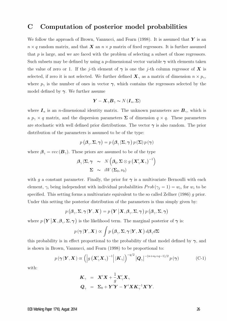
C Computation of posterior model probabilities

We follow the approach of Brown, Vannucci, and Fearn (1998). It is assumed that Y is an

n× q random matrix, and that X an n× p matrix of fixed regressors. It is further assumed

that p is large, and we are faced with the problem of selecting a subset of those regressors.

Such subsets may be defined by using a p-dimensional vector variable γ with elements taken

the value of zero or 1. If the j-th element of γ is one the j-th column regressor of X is

selected, if zero it is not selected. We further defined Xγ as a matrix of dimension n × pγ,where pγ is the number of ones in vector γ, which contains the regressors selected by the

model defined by γ. We further assume

Y −XγBγ ∼ N (In,Σ)

where In is an n-dimensional identity matrix. The unknown parameters are Bγ, which is

a pγ × q matrix, and the dispersion parameters Σ of dimension q × q. These parameters

are stochastic with well defined prior distributions. The vector γ is also random. The prior

distribution of the parameters is assumed to be of the type:

p(βγ,Σ,γ

)= p

(βγ |Σ,γ

)p (Σ) p (γ)

where βγ = vec (Bγ). These priors are assumed to be of the type

βγ |Σ,γ ∼ N(β0,Σ⊗ g

(X ′γXγ

)−1)

Σ ∼ iW (Σ0, ν0)

with g a constant parameter. Finally, the prior for γ is a multivariate Bernoulli with each

element, γi being independent with individual probabilities Prob (γj = 1) = wi, for wi to be

specified. This setting forms a multivariate equivalent to the so called Zellner (1986) g prior.

Under this setting the posterior distribution of the parameters is thus simply given by:

p(βγ,Σ,γ |Y ,X

)= p

(Y∣∣X,βγ,Σ,γ

)p(βγ,Σ,γ

)where p

(Y∣∣X,βγ,Σ,γ

)is the likelihood term. The marginal posterior of γ is:

p (γ |Y ,X ) ∝∫p(βγ,Σ,γ |Y ,X

)dβγdΣ

this probability is in effect proportional to the probability of that model defined by γ, and

is shown in Brown, Vannucci, and Fearn (1998) to be proportional to:

p (γ |Y ,X ) ∝(∣∣∣g (X ′γXγ

)−1∣∣∣ |Kγ|

)−q/2 ∣∣Qγ

∣∣−(n+ν0+q−1)/2p (γ) (C-1)

with:

Kγ = X ′X +1

gX ′γXγ

Qγ = Σ0 + Y ′Y − Y ′XK−1γ X

′Y .


Table 1: Least Square estimation results of CDS pricing model.

France Germany Greece Ireland Italy Portugal Spain

α1 -0.0001 0.0000 0.0010 0.0018 0.0001 -0.0001 0.0002α2 0.0011 -0.0002 0.0000 0.0003 -0.0216 0.0000 -0.0006β1 1.0238 1.0083 1.0036 0.9925 0.9865 1.0215 0.9978β2 1.0058 0.9997 1.0047 1.0041 0.9645 1.0268 0.9978

σxx 4.4E-06 1.1E-06 7.4E-07 6.6E-07 1.3E-05 2.3E-05 2.2E-05σzz 2.0E-05 8.4E-12 2.2E-06 4.4E-06 1.9E-05 3.5E-03 8.3E-07σxz 1.6E-10 -1.2E-10 -2.6E-07 1.6E-06 -3.9E-08 2.1E-05 1.9E-06σuu 4.0E-04 3.1E-06 1.2E-03 3.4E-06 2.4E-04 5.3E-01 6.6E-06

x0 -0.005 -0.011 -0.002 -0.021 0.025 0.001 0.025z0 1.160 -1.436 1.238 -1.707 -2.150 0.748 -1.975

ρxz 0.000 -0.041 -0.200 0.943 -0.002 0.073 0.443

R2 0.94 0.86 0.98 0.98 0.91 0.89 0.97S.E. 0.25 0.37 0.40 0.24 0.31 0.64 0.22

MAV 4.1 6.5 46.9 17.8 15.4 38.7 11.5

Note: α1, α2, β1, and β2 are the parameters of the state equation in model 5. σab denotes covariance

between a and b, x0 and z0 are the respective starting values of x and z. ρxz is the correlation between

the unobservable factors x and z. R2 is computed as one minus the ratio of the sum of squared residuals

over the sum of squared dependent variables. S.E. denotes the residual standard error. Finally, MAV is

the mean absolute value of the error term in basis points. Standard errors of the estimated parameters,

computed by means of Monte Carlo simulations of the model, are shown in Table 2.


Table 2: Simulations of the CDS models

α1 α2 β1 β2 σxx σzz σxz σuu x0 z0

Germany true 0.00003 -0.00025 1.00830 0.99974 1.077E-06 8.390E-12 -1.245E-10 3.07522E-06 -0.0107 -1.4357mean 0.00003 -0.00025 1.00917 0.99703 1.070E-06 8.538E-12 -1.256E-10 3.1256E-06 -0.0108 -1.4486median 0.00003 -0.00025 1.00543 0.99824 1.077E-06 8.545E-12 -1.253E-10 3.14834E-06 -0.0108 -1.4465S.D. 0.00000 0.00001 0.01223 0.00512 4.820E-08 2.246E-13 3.266E-12 1.07125E-07 0.0002 0.0340relative error 2.4% 2.0% 1.2% 0.5% 4.5% 2.7% 2.6% 3.5% 2.0% 2.4%

France true -0.00006 0.00107 1.02376 1.00580 4.420E-06 2.032E-05 1.597E-10 0.00040 -0.0054 1.1602mean -0.00005 0.00107 1.03375 1.00702 4.567E-06 2.107E-05 1.612E-10 0.00039 -0.0054 1.2143median -0.00006 0.00108 1.03136 1.00292 4.455E-06 2.048E-05 1.607E-10 0.00040 -0.0054 1.1744S.D. 0.00000 0.00008 0.01956 0.00805 4.647E-07 2.436E-06 1.811E-11 6.15855E-05 0.0003 0.1024relative error 7.4% 7.6% 1.9% 0.8% 10.5% 12.0% 11.3% 15.5% 5.9% 8.8%

Greece true 0.00099 0.00000 1.00358 1.00468 7.361E-07 2.230E-06 -2.565E-07 0.00120 -0.0024 1.2384mean 0.00100 0.00000 1.01748 1.00561 7.408E-07 2.256E-06 -2.596E-07 0.00121 -0.0024 1.2396median 0.00100 0.00000 1.01651 1.00570 7.385E-07 2.251E-06 -2.585E-07 0.00121 -0.0024 1.2432S.D. 0.00002 0.00000 0.00939 0.00209 3.793E-08 8.978E-08 9.426E-09 4.472E-05 0.0001 0.0304relative error 2.3% 3.0% 0.9% 0.2% 5.2% 4.0% 3.7% 3.7% 2.4% 2.5%

Ireland true 0.00181 0.00035 0.99249 1.00409 6.554E-07 4.429E-06 1.606E-06 3.403E-06 -0.0207 -1.7069mean 0.00183 0.00034 1.00060 1.00511 6.385E-07 4.509E-06 1.584E-06 3.305E-06 -0.0219 -1.6868median 0.00184 0.00035 0.99174 1.00401 6.500E-07 4.495E-06 1.606E-06 3.370E-06 -0.0214 -1.7076S.D. 0.00012 0.00005 0.01914 0.00274 6.278E-08 5.333E-07 1.415E-07 5.852E-07 0.0019 0.0907relative error 6.6% 13.3% 1.9% 0.3% 9.6% 12.0% 8.8% 17.2% 9.0% 5.3%

Italy true 0.00006 -0.02164 0.98650 0.96454 1.266E-05 1.937E-05 -3.881E-08 0.00024 0.0246 -2.1503mean 0.00006 -0.02184 0.97888 0.97491 1.275E-05 1.964E-05 -3.922E-08 0.00025 0.0248 -2.1501median 0.00006 -0.02181 0.98085 0.97643 1.272E-05 1.959E-05 -3.900E-08 0.00025 0.0248 -2.1548S.D. 0.00000 0.00070 0.02129 0.01001 4.933E-07 5.242E-07 1.476E-09 7.129E-06 0.0006 0.0473relative error 1.9% 3.3% 2.2% 1.0% 3.9% 2.7% 3.8% 2.9% 2.4% 2.2%

Portugal true -0.00007 0.00000 1.02148 1.02677 2.304E-05 3.465E-03 2.060E-05 0.53206 0.0015 0.7478mean -0.00007 0.00000 1.03057 1.02253 2.054E-05 4.010E-03 1.878E-05 0.51163 0.0015 0.8619median -0.00007 0.00000 1.02846 1.02206 2.288E-05 3.503E-03 2.052E-05 0.53208 0.0015 0.7579S.D. 0.00002 0.00000 0.01870 0.01156 7.058E-06 1.744E-03 5.089E-06 0.20584 0.0005 0.2136relative error 29.6% 19.3% 1.8% 1.1% 30.6% 50.3% 24.7% 38.7% 31.9% 28.6%

Spain true 0.00019 -0.00059 0.99775 0.99780 2.209E-05 8.267E-07 1.891E-06 6.570E-06 0.0252 -1.9754mean 0.00019 -0.00060 1.00532 0.99823 2.282E-05 8.368E-07 1.903E-06 6.580E-06 0.0251 -1.9862median 0.00019 -0.00060 0.99980 0.99827 2.267E-05 8.251E-07 1.916E-06 6.649E-06 0.0253 -1.9815S.D. 0.00001 0.00003 0.01939 0.00370 1.544E-06 4.966E-08 8.079E-08 4.225E-07 0.0012 0.0482relative error 7.7% 4.9% 1.9% 0.4% 7.0% 6.0% 4.3% 6.4% 4.9% 2.4%

Note: α1, α2, β1, and β2 are the parameters of the state equation in model 5. σab denotes covariance between a and b, x0 and z0 are the respective

starting values of x and z. ”True” are the estimated parameter values used in simulations. ”Mean”, ”Median”, and ”S.D.” are mean, median, standard

deviations of estimated parameters from a number of simulations. ”relative error” is the standard deviation divided by the true parameter value. 100

simulations were run for each model.


Table 3: Key events and news in the euro area during the financial crisis.

Date Description Grouping

Institutional Developments

Aug-2007 ECB provides liquidity assistance to calm tensions in interbank market Market functioningJan-2008 US and EA economic indicators point to recession Ec & Fiscal StimulusMar-2008 ECB offers refinancing operations with longer maturities Market FunctioningJul-2008 ECB increases interest rates by 25 bps Standard MPSep-2008 Lehman Brothers files for bankruptcy Lehman BrothersOct-2008 Unlimited liquidity provision of ECB to banks Market Functioning

Launch of national bail-out plans for banks Bank SupportECB cut rates by 50 bps Standard MP

Nov-2008 Announcement of European Economic Recovery Plan Ec & Fiscal StimulusECB cuts rates by 50 bps Standard MP

Dec-2008 ECB cuts rates by 75 bps Standard MPJan-2009 ECB cuts rates by 50 bps Standard MPMar-2009 ECB cuts rates by 50 bps Standard MPApr-2009 ECB cuts rates by 25 bps Standard MPMay-2009 Announcement of European Financial Supervision Plan Support BanksJun-2009 ECB launches covered bond programme Market FunctioningMay-2010 ECB announces Securities Markets Programme Market FunctioningJun-2010 European Financial Stability Facility launched Government SupportJul-2010 EU banks stress tests published Bank SupportJun-2010 Effective lending capacity of EFSF is increased Government SupportJul-2011 EU banks stress tests published Bank Support

ECB increases rates by 25 bps Standard MPAug-2011 ECB’s SMP programme is extended to Spain and Italy Market FunctioningDec-2011 ECB announces additional non-standard measures (3-year LTRO) Market Functioning

EU agrees on new fiscal compact limiting structural deficits Ec & Fiscal StimulusJun-2012 EU Council announces Compact for Growth and Jobs Ec & Fiscal StimulusJul-2012 President Draghi London speech in support of Euro Market Functioning

Country News

Nov-2009 Greek announces public deficit would exceed 12% News GreeceApr-2010 announcement of EU/IMF financial support for Greece News GreeceOct-2010 Speculation on EU discussions on possible debt restructuring News IrelandNov-2010 Irish government seeks financial support News IrelandDec-2010 Irish package is agreed News IrelandApr-2011 Portuguese government requests activation of aid mechanism News PortugalJun-2011 DE and FR agree on need for PSI in Greek crisis News GreeceJul-2011 Eurogroup sets PSI as precondition for further aid to GR News GreeceOct-2011 Restructuring on GR debt deemed larger than previously envisaged News GreeceNov-2011 Announcement of referendum in Greece on aid assistance News GreeceMar-2012 Agreement on the (PSI) restructuring of Greek debt News Greece

Note: bps are used to denote basis points.


Table 4: BMA regression results.Germany France Greece Ireland Italy Portugal Spain

PD LGD PD LGD PD LGD PD LGD PD LGD PD LGD PD LGD

With ‘permanent-effect dummies’

VIX - 0.03∗∗ - - 0.03∗∗ 0.17∗∗ - - - - - 0.08∗∗ - 0.04∗∗

VSP - - - - - - - - - - - - - -RAT - - - - 0.23∗∗ - - - - - 0.39∗∗ - - -iTraxx 0.61∗∗ - 0.42∗∗ - 0.39∗∗ 0.21∗∗ - - 0.66∗∗ - - 0.07∗∗ 0.57∗∗ -BCDS - - - -0.20∗∗ - -0.03∗∗ - - - - - - - -FUT-SER - - - - - - - - - 0.04∗∗ - - - -FUT-GDP - - - 0.17∗∗ - - - - - - - - - -DEF - - - - - - -0.04∗∗ - - - - - - -BC - - - - - - - - - - - - - -

Market Functioning - -0.04∗∗ - - - - - - - - - - - -Standard MP - - - - - - - - - - - - - -Government Support - - - - 0.12∗∗ - 0.03∗∗ - - - - - - -Bank Support - - - - - - - - - - - - - -Ec & Fiscal Stimulus - 0.03∗∗ - - - - - - - - - -0.11∗∗ - -Lehman Brothers - - 0.21∗∗ - - - - 0.27∗∗ - - - - - 0.07∗∗

News Greece - - - - - - - - - - - - - 0.05∗∗

News Ireland - - - - - - - - - - - - - -News Portugal - - - - 0.27∗∗ - 0.03∗∗ - - - - - - -

R2 0.37 0.05 0.31 0.20 0.38 0.23 0.04 0.09 0.44 0.03 0.16 0.12 0.33 0.06

With ‘temporary-effect dummies’

VIX - - 0.13∗∗ - 0.08∗∗ 0.17∗∗ - 0.02∗∗ - - - 0.16∗∗ - 0.10∗∗

VSP - - - - - - - - - - - - - -RAT - - - - 0.28∗∗ - - - - - 0.39∗∗ - - -iTraxx 0.60∗∗ - 0.31∗∗ - 0.18∗∗ 0.20∗∗ - - 0.65∗∗ - - 0.20∗∗ 0.57∗∗ -BCDS - - - -0.20∗∗ - -0.03∗∗ - - - - - - - -FUT-SER - - - - - - - - - - - - - -FUT-GDP - - - 0.17∗∗ - - - - - - - - - -DEF - - - - - - - - - - - - - -BC - - - - - - - - - - - - - -

Market Functioning - - - - - - - - - - - - - -Standard MP - - - - - - - - - - - - - -Government Support - - - - - - - - - - - - - -Bank Support - - - - - - - - - - - - - -Ec & Fiscal Stimulus 0.14∗∗ - - - - - - - - - - - - -Lehman Brothers - - 0.13∗∗ - - - - - - -0.16∗∗ - - - -

News Greece - - - - - - - - - - - - - -News Ireland - - - - - - -0.43∗∗ 0.44∗∗ - - - - - -News Portugal - - - - - - - - - - - - - -

R2 0.37 0.08 0.29 0.21 0.29 0.23 0.19 0.25 0.43 0.04 0.15 0.18 0.33 0.04

Note: Data has been normalised, results in the table relate to regressions conducted for the two-year PDs and LGDs. Values reported for the regression

coefficients are only those significant and larger than 0.01. ∗ denotes significance at a 5% level of significance.


Table 5: Contagion across sovereign markets. Correlation of residuals.

With ‘permanent-effect dummies’

PD residuals LGD residuals

France Germany Greece Ireland Italy Portugal France Germany Greece Ireland Italy Portugal

Germany 0.57* 0.43*Greece -0.09 0.08 0.35* 0.01Ireland 0.21 0.22 0.03 0.16 0.20 0.17Italy 0.20 0.37* 0.06 0.10 -0.08 -0.05 -0.08 -0.16Portugal 0.27* 0.15 -0.06 0.00 0.19 -0.08 -0.14 -0.11 0.31* -0.04Spain 0.14 0.14 -0.24 0.21 0.34* 0.19 0.38* 0.19 0.30* 0.28* -0.18 0.23

With ‘temporary-effect dummies’

PD residuals LGD residuals

France Germany Greece Ireland Italy Portugal France Germany Greece Ireland Italy Portugal

Germany 0.57* 0.46*Greece -0.13 0.04 0.35* 0.02Ireland 0.23 0.19 -0.04 0.17 0.21 0.09Italy 0.20 0.38* 0.04 0.19 -0.08 -0.08 -0.09 -0.19Portugal 0.27* 0.15 -0.09 0.03 0.19 -0.07 -0.19 -0.12 0.28* -0.05Spain 0.14 0.14 -0.21 0.33* 0.35* 0.19 0.39* 0.20 0.30* 0.35* -0.18 0.20

Note: Correlations significant at the 5% level are denoted with an asterisk. Correlations have been computed with residuals of regressions of PD

and LGD within 2 year maturity.


Figure 1: PD and LGD combinations providing model-implied CDS spreads which fit per-fectly the observed CDS spreads over different maturities on December 2010.

0.02 0.04 0.06 0.08 0.1 0.12 0.140.05

0.1

0.15

0.2

0.25

0.3

0.35

0.4

Germany

PD

LGD

0.04 0.06 0.08 0.1 0.12 0.14 0.16

0.1

0.2

0.3

0.4

0.5

0.6

0.7

France

PD

LGD

0.3 0.4 0.5 0.6 0.7 0.8 0.9

0.1

0.2

0.3

0.4

0.5

0.6

Greece

PD

LGD

0.2 0.3 0.4 0.5 0.60.1

0.2

0.3

0.4

0.5

0.6

0.7

0.8

Ireland

PD

LGD

0.1 0.2 0.3 0.4 0.5

0.2

0.4

0.6

0.8

Italy

PD

LGD

0.05 0.1 0.15 0.2 0.25

0.2

0.3

0.4

0.5

0.6

0.7

0.8

Portugal

PD

LGD

0.3 0.4 0.5 0.6 0.7 0.8

0.05

0.1

0.15

0.2

0.25Spain

PD

LGD

1−year3−year7−year10−year


Figure 2: PD and LGD combinations providing model-implied CDS spreads within the esti-mated mean absolute error from observed CDS spreads over different maturities on December2010.

Germany

PD

LGD

0.02 0.04 0.06 0.08 0.1 0.12 0.140.05

0.1

0.15

0.2

0.25

0.3

0.35

0.4

France

PD

LGD

0.04 0.06 0.08 0.1 0.12 0.14 0.16

0.2

0.4

0.6

0.8

Greece

PD

LGD

0.3 0.4 0.5 0.6 0.7 0.8 0.9

0.1

0.2

0.3

0.4

0.5

0.6

Ireland

PD

LGD

0.2 0.3 0.4 0.5 0.6

0.2

0.4

0.6

0.8

Italy

PD

LGD

0.1 0.2 0.3 0.4 0.5

0.2

0.4

0.6

0.8

Portugal

PD

LGD

0.05 0.1 0.15 0.2 0.25

0.2

0.3

0.4

0.5

0.6

0.7

0.8

Spain

PD

LGD

0.3 0.4 0.5 0.6 0.7 0.8

0.05

0.1

0.15

0.2

0.25


Figure 3: PD and LGD within 2 years.

0

0.2

0.4

0.6

0.8

1

Jan-2008 Aug-2008 Mar-2009 Oct-2009 May-2010 Dec-2010 Jul-2011 Feb-2012

PDs

0

0.1

0.2

0.3

0.4

0.5

0.6

0.7

Jan-2008 Aug-2008 Mar-2009 Oct-2009 May-2010 Dec-2010 Jul-2011 Feb-2012

LGDs

DE GR IE IT FR PT SP


Figure 4: Coincidences of large residuals. With ‘permanent-effect dummies ’.

0%

20%

40%

60%

80%

100%

Jan-2008 Jan-2009 Jan-2010 Jan-2011 Jan-2012

PD

0%

20%

40%

60%

80%

100%

Jan-2008 Jan-2009 Jan-2010 Jan-2011 Jan-2012

LGD

Note: Coincidences are measured as the ratio of the number of residual values above their empirical 75th percentiles to thetotal number of the analysed countries in a given period. The residual values are estimated from the regressions of changes inPD (top chart) and LGD (bottom chart) on the set of economic fundamentals as explained in the main text.


market perception of sovereign credit risk in the euro area during the

Documents