mapping functional diversity from remotely sensed...
TRANSCRIPT

ARTICLE
Mapping functional diversity from remotely sensedmorphological and physiological forest traitsFabian D. Schneider 1, Felix Morsdorf 1, Bernhard Schmid 2, Owen L. Petchey 2, Andreas Hueni 1,
David S. Schimel 3 & Michael E. Schaepman 1
Assessing functional diversity from space can help predict productivity and stability of forest
ecosystems at global scale using biodiversity–ecosystem functioning relationships. We pre-
sent a new spatially continuous method to map regional patterns of tree functional diversity
using combined laser scanning and imaging spectroscopy. The method does not require prior
taxonomic information and integrates variation in plant functional traits between and within
plant species. We compare our method with leaf-level field measurements and species-level
plot inventory data and find reasonable agreement. Morphological and physiological diversity
show consistent change with topography and soil, with low functional richness at a mountain
ridge under specific environmental conditions. Overall, functional richness follows a loga-
rithmic increase with area, whereas divergence and evenness are scale invariant. By mapping
diversity at scales of individual trees to whole communities we demonstrate the potential of
assessing functional diversity from space, providing a pathway only limited by technological
advances and not by methodology.
DOI: 10.1038/s41467-017-01530-3 OPEN
1 Remote Sensing Laboratories, Department of Geography, University of Zurich, Winterthurerstrasse 190, CH-8057 Zurich, Switzerland. 2 Department ofEvolutionary Biology and Environmental Studies, University of Zurich, Winterthurerstrasse 190, CH-8057 Zurich, Switzerland. 3 Jet Propulsion Laboratory,California Institute of Technology, 4800 Oak Grove Drive, Pasadena, CA 91011, USA. Correspondence and requests for materials should be addressed toF.D.S. (email: [email protected])
NATURE COMMUNICATIONS |8: 1441 |DOI: 10.1038/s41467-017-01530-3 |www.nature.com/naturecommunications 1
1234
5678
90

Understanding community structure and the impact ofchanging biodiversity on ecosystem functioning are keytasks in ecology. Progress has been made on a wide variety
of taxa, including plants1, fish2, birds3 and insects4, amongstothers. In plant ecology, biodiversity research has focused on thedistribution of species based on taxonomic identity5. Morerecently, with the emergence of functional biogeography6, treespecies or individuals of a community are described in relation totheir functional identity and distribution in space. Functionaltraits are of particular interest due to their response to environ-mental conditions and direct link to growth, reproduction andsurvival7, 8. Trait-based approaches are emerging rapidly in plantecology, underpinning community assembly and structure, spe-cies interactions and interlinkages between vegetation and bio-geochemical cycles9.
The assessment of plant functional traits and plant functionaldiversity is of particular relevance when predicting ecosystemproductivity and stability. A multitude of experimental studiesdemonstrated positive relationships between plant diversity andecosystem functioning10–12 and increasingly such positive rela-tionships are also found in comparative observational studies13,14. A positive relationship over extended time scales is mainlydriven by functional diversity due to an increased resource useefficiency and utilization as well as sampling effects in a changingenvironment, allowing plant communities to sustain high pro-ductivity over time15–17. Besides productivity, higher functionaldiversity has been linked to enhanced tree growth and ecosystemstability due to complementarity effects, better adaptability tochanging environmental conditions and lower vulnerability todiseases, insect attacks, fire and storms18–20. However, to makeuse of the increasing knowledge about biodiversity–ecosystemfunctioning relationships in forest ecosystems, it would benecessary to develop methods to assess plant functional diversityefficiently over large continuous areas. Our first aim is thereforeto develop such a method for a regional test area, see Fig. 1, as abase for larger scale biodiversity scoping studies.
Spatial variation in plant functional traits and diversity dependon community structure21 and thus represent a potential signal ofcommunity assembly processes. However, plant traits and func-tional diversity do not only depend on community structurerepresented by particular species abundance distributions withina specific geographical unit, but may vary as much within speciesas they do between species22. Different species can also beredundant in terms of their functional traits, and thus not con-tribute to functional diversity16, 23. Therefore, functional diversityis best derived from a given set of traits including their intra-specific variability24, 25. By incorporating individual-level func-tional traits, functional diversity may better predict ecosystemfunctioning than species-level means16.
A multitude of forest monitoring networks exist26 as well astrait-based studies in forested ecosystems27, fostered by standar-dized measurement procedures28 and global trait databases29.However, these procedures usually require taxonomic informa-tion about tree individuals and indirectly assess trait variation andfunctional diversity combining information about species abun-dances and mean traits, thus ignoring variation in tree functionaltraits within species, which can be large even within individuals30.In addition, there is a global bias in the distribution of forestplots, leading to large data gaps particularly in remote areas31.Furthermore, trait measurements in forests are typically limitedin extent and magnitude due to the complexity of destructivecrown-level measurements, as well as associated georeferencingchallenges and plot representativeness32. Consequently, con-tinuous spatial data of traits and especially on trait diversity arestill very sparse. Recent advances in remote sensing provide theopportunity to map traits and trait diversity, thus filling the
existing data gaps33–35. Here, we use three morphological andthree physiological functional traits that we assess directly, i.e.without reference to taxonomic information, to provide a spa-tially continuous description of functional diversity in a forest atlocal scale (≈925 ha), with the potential to scale up to regionaland to the global level.
The selected morphological and physiological traits can beassessed with high-resolution airborne remote sensing methods33,36 and are relevant for plant and ecosystem function. Threemorphological traits, namely canopy height (CH, vertical distancebetween canopy top and ground), plant area index (PAI, pro-jected plant area per horizontal ground area) and foliage heightdiversity (FHD, measure of variation and number of canopylayers), are essential to describe canopy architecture, encom-passing the horizontal and vertical structure of forests andinfluencing light availability, thus affecting competitive andcomplementary light use and ecosystem productivity18, 37. Threephysiological traits, namely leaf chlorophyll (CHL, relative con-tent of chlorophyll a+b per unit leaf area), leaf carotenoids (CAR,relative content of carotenoids per unit leaf area) and equivalentwater thickness (EWT, leaf water content per unit leaf area), donot modify light availability but rather describe light use at thelevel of single leaves. The chlorophylls are functionally importantpigments, since they control the amount of photosyntheticallyactive radiation absorbed for photosynthesis38. Carotenoids arecontributing to the chlorophylls by absorbing additional radiationfor photosynthesis and protecting leaves from over-exposition tohigh amounts of incoming solar radiation by releasing excessenergy38. The third, EWT, is important for plant responses todrought, which could reduce the physiological performancethrough decreased photosynthetic carbon assimilation and elec-tron transport rate39.
We use the above traits to derive measures of functionaldiversity separately for the morphological and leaf physiologicaltraits. Our functional diversity measures are combining multipletraits, as is typically done for such measures23. We calculate threemeasures, related to different aspects of functional diversity—functional richness, divergence and evenness40, 41. Functional
Southern slope
Northern slope
Flat areas
A
B
C
Fig. 1 Laegern mountain temperate mixed forest site in Switzerland. Thetest site is located near Zurich and covers about 2 × 6 km. The mountainrange is divided by a ridge running from east to west, separating theforested area in north facing (blue) and south facing (orange) slopes. Flatareas are defined with a slope <10° (green). Areas not covered by forest(agriculture, grassland, urban areas) are shown in grey
ARTICLE NATURE COMMUNICATIONS | DOI: 10.1038/s41467-017-01530-3
2 NATURE COMMUNICATIONS | 8: 1441 |DOI: 10.1038/s41467-017-01530-3 |www.nature.com/naturecommunications

richness is calculated as the convex hull volume of the communityniche42, as illustrated in Fig. 2a for an assemblage of pixelsmapped in the morphological trait space. It corresponds to theniche extent and defines the outer boundary of the occupiedfunctional space. A disadvantage of this measure may be a stronginfluence by extreme values. In contrast, functional divergenceand evenness describe how sample points are distributed withinthe community niche (Fig. 2b, c). Functional divergence is ameasure of how sample points are spread with regard to the meandistance to the centre of gravity, whereas functional evennessindicates how evenly traits are distributed with regard to spacingamong similar sample points in functional space. These threeindices have mainly been applied to functional diversity ofplants43, where sample points represent species, with anincreasing number of studies on forest ecosystems44. However,this concept has not yet been applied to continuously measuredtrait data independent of taxonomy, vegetation units or evenplant individuals. Remote sensing methods offer to measurefunctional traits continuously and directly across large spatialextents. This has a twofold advantage: (1) there is no need toidentify species, vegetation units or individuals and (2) predictionof ecosystem functions using independently established func-tional diversity–ecosystem functioning relationships are con-sistent across large scales. In contrast, recent efforts to map forestbiodiversity have used forest functional classes as remotely sensedvegetation units with constant trait values assigned to theseunits35.
Our second aim is to test the consistency of our method. Forthis, we compare the results obtained with the two independentsets of traits. Morphological diversity was found to be the maindriver of forest productivity in poly- and monocultures of matureforests45–47, whereas physiological diversity reflects differentresource allocation strategies to maximize light capture andprotective mechanisms and is more closely linked to speciesdiversity48, 49. Since most functional traits show consistent var-iation along broad environmental gradients, we expect bothmorphological and physiological diversity to show similar pat-terns at larger scales. For the leaf physiological traits, we alsocompare the remotely sensed trait values with those directlyobtained from spectroscopic measurements on single leaves. Thisshould indicate how well the retrieval method can be scaled fromthe leaf to the canopy level. Furthermore, we test the generalagreement of trends in trait relationships between communityweighted means of the functional trait database TRY and theretrieved traits for communities composed of the 13 tree speciespresent in our test area.
Finally, we examine scale dependency of different functionaldiversity measures. We demonstrate that functional diversitymeasures can be quantified at any desired unit area within thesampled region, limited only by the spatial resolution of the traitmaps. This will allow—in future efforts—for direct and con-tinuous mapping of functional diversity from space. Functionaldiversity, due to redundancy and trait plasticity, may not showthe same increase with area as is typically found for speciesrichness. Nevertheless, scale dependency of functional diversitycould still lead to scale-dependent functional diversity–ecosystemfunctioning relationships. Such effects would be expected if eco-system functions are not scale-dependent above a certain mini-mum area, which is likely the case, such as for example forproductivity per area. Studies on spatial patterns and scaledependency of functional diversity are still sparse50. We expectfunctional richness to increase with scale. A strong increase atsmall scales would indicate high diversity within communities,which can mean higher resilience to disturbance51, while anincrease at larger scales would indicate high diversity betweencommunities. The exact slope and shape of the relationship,however, cannot be predicted by known species–area relation-ships, since functional richness is influenced by trait correlations,redundancies among species and intra-specific trait variation.Even less is known about other components of functionaldiversity. A study based on four plant communities on the San-torini Archipelago found no relationship with area for functionaldivergence and evenness52.
ResultsFunctional traits. Figure 3 shows the spatial distribution ofmorphological and physiological traits, as derived from airbornelaser scanning and airborne imaging spectroscopy, respectively.Blue areas in the morphological trait map are characterized byhigh canopy density, low canopy height and little canopy layering.When comparing with independent community data, around83% of these areas are classified as juvenile forest with tree heightbelow 21 m and diameter at breast height below 30 cm (Supple-mentary Fig. 1). The largest such area is marked as subregion A,covering ∼1.4 ha, and is likely affected by disturbance caused by awinter storm. Physiologically, these patches are characterized byvery high chlorophyll concentration as compared to an undis-turbed, mature forest canopy.
Larger patches with a dense and closed canopy as well as highrelative chlorophyll and carotenoids content are represented bypink and orange areas in the morphological and physiological
Richness = 0.22F
olia
ge h
eigh
t div
ersi
ty [0
–1]
Fol
iage
hei
ght d
iver
sity
[0–1
]
0.0
0.2
0.4
0.6
0.8
1.0
Divergence = 0.81
0.0
0.2
0.4
0.6
0.8
1.0
Evenness = 0.81
1.00.8
0.6Fol
iage
hei
ght d
iver
sity
[0–1
]
0.40.0
0.2
0.4
0.6
0.8
1.0
0.20.00.00.20.40.60.81.0
Plant area index [0–1] Canopy height [0
–1]1.0
0.80.6
0.40.2
0.00.00.20.40.60.81.0
Plant area index [0–1]0.00.20.40.60.81.0
Plant area index [0–1] Canopy height [0
–1]
1.00.8
0.60.4
0.20.0
Canopy height [0
–1]
b ca
Fig. 2 Three aspects of functional diversity based on morphological forest traits of a circular area with a radius of 120m. The three traits are foliage heightdiversity, plant area index and canopy height in relative units from 0 to 1. a The shaded volume is functional richness, b the distance from the surface of theshaded sphere is functional divergence and c the variation of segment length in the minimum spanning tree is functional evenness
NATURE COMMUNICATIONS | DOI: 10.1038/s41467-017-01530-3 ARTICLE
NATURE COMMUNICATIONS |8: 1441 |DOI: 10.1038/s41467-017-01530-3 |www.nature.com/naturecommunications 3
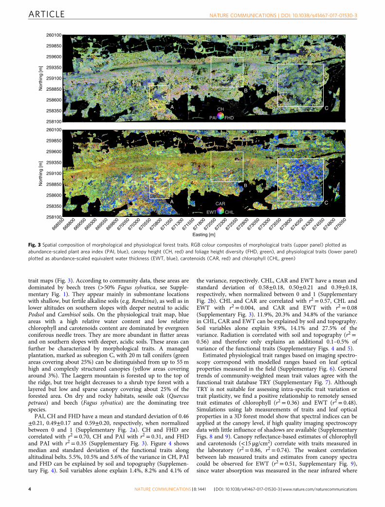
trait maps (Fig. 3). According to community data, these areas aredominated by beech trees (>50% Fagus sylvatica, see Supple-mentary Fig. 1). They appear mainly in submontane locationswith shallow, but fertile alkaline soils (e.g. Rendzina), as well as inlower altitudes on southern slopes with deeper neutral to acidicPodsol and Cambisol soils. On the physiological trait map, blueareas with a high relative water content and low relativechlorophyll and carotenoids content are dominated by evergreenconiferous needle trees. They are more abundant in flatter areasand on southern slopes with deeper, acidic soils. These areas canfurther be characterized by morphological traits. A managedplantation, marked as subregion C, with 20 m tall conifers (greenareas covering about 25%) can be distinguished from up to 55 mhigh and complexly structured canopies (yellow areas coveringaround 3%). The Laegern mountain is forested up to the top ofthe ridge, but tree height decreases to a shrub type forest with alayered but low and sparse canopy covering about 25% of theforested area. On dry and rocky habitats, sessile oak (Quercuspetraea) and beech (Fagus sylvatica) are the dominating treespecies.
PAI, CH and FHD have a mean and standard deviation of 0.46±0.21, 0.49±0.17 and 0.59±0.20, respectively, when normalizedbetween 0 and 1 (Supplementary Fig. 2a). CH and FHD arecorrelated with r2= 0.70, CH and PAI with r2= 0.31, and FHDand PAI with r2= 0.35 (Supplementary Fig. 3). Figure 4 showsmedian and standard deviation of the functional traits alongaltitudinal belts. 5.5%, 10.5% and 5.6% of the variance in CH, PAIand FHD can be explained by soil and topography (Supplemen-tary Fig. 4). Soil variables alone explain 1.4%, 8.2% and 4.1% of
the variance, respectively. CHL, CAR and EWT have a mean andstandard deviation of 0.58±0.18, 0.50±0.21 and 0.39±0.18,respectively, when normalized between 0 and 1 (SupplementaryFig. 2b). CHL and CAR are correlated with r2 = 0.57, CHL andEWT with r2= 0.004, and CAR and EWT with r2 = 0.08(Supplementary Fig. 3). 11.9%, 20.3% and 34.8% of the variancein CHL, CAR and EWT can be explained by soil and topography.Soil variables alone explain 9.9%, 14.1% and 27.5% of thevariance. Radiation is correlated with soil and topography (r2=0.56) and therefore only explains an additional 0.1–0.5% ofvariance of the functional traits (Supplementary Figs. 4 and 5).
Estimated physiological trait ranges based on imaging spectro-scopy correspond with modelled ranges based on leaf opticalproperties measured in the field (Supplementary Fig. 6). Generaltrends of community-weighted mean trait values agree with thefunctional trait database TRY (Supplementary Fig. 7). AlthoughTRY is not suitable for assessing intra-specific trait variation ortrait plasticity, we find a positive relationship to remotely sensedtrait estimates of chlorophyll (r2= 0.36) and EWT (r2= 0.48).Simulations using lab measurements of traits and leaf opticalproperties in a 3D forest model show that spectral indices can beapplied at the canopy level, if high quality imaging spectroscopydata with little influence of shadows are available (SupplementaryFigs. 8 and 9). Canopy reflectance-based estimates of chlorophylland carotenoids (<15 μg/cm2) correlate with traits measured inthe laboratory (r2= 0.86, r2= 0.74). The weakest correlationbetween lab measured traits and estimates from canopy spectracould be observed for EWT (r2= 0.51, Supplementary Fig. 9),since water absorption was measured in the near infrared where
Nor
thin
g [m
]
Easting [m]
Nor
thin
g [m
]
PAI FHD
CH
EWT CHL
CAR
A
B
C
A
B
C
258100
258350
258600
258850
259100
259350
259600
259850
260100
258100
258350
258600
258850
259100
259350
259600
259850
260100
6685
50
6688
00
6690
50
6693
00
6695
50
6698
00
6700
50
6703
00
6705
50
6708
00
6710
50
6713
00
6715
50
6718
00
6720
50
6723
00
6725
50
6728
00
6730
50
6733
00
6735
50
6738
00
6740
50
6743
00
6745
50
6748
00
6750
50
Fig. 3 Spatial composition of morphological and physiological forest traits. RGB colour composites of morphological traits (upper panel) plotted asabundance-scaled plant area index (PAI, blue), canopy height (CH, red) and foliage height diversity (FHD, green), and physiological traits (lower panel)plotted as abundance-scaled equivalent water thickness (EWT, blue), carotenoids (CAR, red) and chlorophyll (CHL, green)
ARTICLE NATURE COMMUNICATIONS | DOI: 10.1038/s41467-017-01530-3
4 NATURE COMMUNICATIONS | 8: 1441 |DOI: 10.1038/s41467-017-01530-3 |www.nature.com/naturecommunications

N 5
12m
N 6
02m
N 6
55m
N 7
12m
N 8
04m
S 8
04m
S 7
12m
S 6
55m
S 6
02m
S 5
12m
0
0.05
0.05
0.1
0.15
0.2
0.15
0.2
0.25
0.3
0.35F
unct
iona
l ric
hnes
s
N 5
12m
N 6
02m
N 6
55m
N 7
12m
N 8
04m
S 8
04m
S 7
12m
S 6
55m
S 6
02m
S 5
12m
0.6
0.7
0.8
0.7
0.8
0.7
0.8
Fun
ctio
nal d
iver
genc
e
N 5
12m
N 6
02m
N 6
55m
N 7
12m
N 8
04m
S 8
04m
S 7
12m
S 6
55m
S 6
02m
S 5
12m
0.7
0.8
0.9
0.8
0.9
0.8
0.9
Fun
ctio
nal e
venn
ess
240
m r
adiu
s60
m r
adiu
s12
m r
adiu
s
N 5
12m
N 6
02m
N 6
55m
N 7
12m
N 8
04m
S 8
04m
S 7
12m
S 6
55m
S 6
02m
S 5
12m
0
0.1
0.2
0.3
0.4
0.5
0.6
0.7
0.8
0.9
1
Fol
iage
hei
ght d
iver
sity
N 5
12m
N 6
02m
N 6
55m
N 7
12m
N 8
04m
S 8
04m
S 7
12m
S 6
55m
S 6
02m
S 5
12m
0
0.1
0.2
0.3
0.4
0.5
0.6
0.7
0.8
0.9
1
Can
opy
heig
ht
N 5
12m
N 6
02m
N 6
55m
N 7
12m
N 8
04m
S 8
04m
S 7
12m
S 6
55m
S 6
02m
S 5
12m
0
0.1
0.2
0.3
0.4
0.5
0.6
0.7
0.8
0.9
1
Pla
nt a
rea
inde
x
Morphology
240
m r
adiu
s60
m r
adiu
s12
m r
adiu
s
Physiology
N 5
12m
N 6
02m
N 6
55m
N 7
12m
N 8
04m
S 8
04m
S 7
12m
S 6
55m
S 6
02m
S 5
12m
0
0.05
0.05
0.1
0.15
0.2
0.25
0.3
0.25
0.3
0.35
0.4
0.45
0.5
Fun
ctio
nal r
ichn
ess
N 5
12m
N 6
02m
N 6
55m
N 7
12m
N 8
04m
S 8
04m
S 7
12m
S 6
55m
S 6
02m
S 5
12m
0.6
0.7
0.8
0.7
0.8
0.7
0.8
Fun
ctio
nal d
iver
genc
e
N 5
12m
N 6
02m
N 6
55m
N 7
12m
N 8
04m
S 8
04m
S 7
12m
S 6
55m
S 6
02m
S 5
12m
0.7
0.8
0.9
0.8
0.9
0.8
0.9
Fun
ctio
nal e
venn
ess
N 5
12m
N 6
02m
N 6
55m
N 7
12m
N 8
04m
S 8
04m
S 7
12m
S 6
55m
S 6
02m
S 5
12m
0
0.1
0.2
0.3
0.4
0.5
0.6
0.7
0.8
0.9
1
Chl
orop
hyll
N 5
12m
N 6
02m
N 6
55m
N 7
12m
N 8
04m
S 8
04m
S 7
12m
S 6
55m
S 6
02m
S 5
12m
0
0.1
0.2
0.3
0.4
0.5
0.6
0.7
0.8
0.9
1
Car
oten
oids
N 5
12m
N 6
02m
N 6
55m
N 7
12m
N 8
04m
S 8
04m
S 7
12m
S 6
55m
S 6
02m
S 5
12m
0
0.1
0.2
0.3
0.4
0.5
0.6
0.7
0.8
0.9
1
Equ
ival
ent w
ater
thic
knes
s
Fig. 4 Boxplots of functional diversity indices and traits grouped by altitudinal belts. Functional richness, divergence and evenness (top panel) are shown forthree spatial scales at 12 m (blue), 60m (purple) and 240m (red) radius. Underlying functional trait values are displayed below, with morphological traitson the left and physiological traits on the right side. Boxes show the median and ±1 standard deviation and whiskers mark ±2 standard deviations. Altitudevalues on the x-axis of the boxplots indicate the middle of the altitudinal belt for the north (N) and the south (S) side of the mountain ridge
0 0.1
A
A
B
B
0.20
0.30.1
AC
C A
B
C
C
B
0.30
0.50.2
0 0.1 0 0.1 0 0.1 0 0.1 0 0.1a b
A B C A B C
Fig. 5 Spatial patterns of morphological and physiological richness at three different scales. Functional richness was computed at 12 m (top), 60m (middle)and 240m (bottom) radius based on a morphological traits and b physiological traits. At 12m radius (top panels), subregions A, B and C are plotted only.The colour is scaled from the lowest (dark blue) to the highest (yellow) richness value with a maximum possible range from 0 to 1
NATURE COMMUNICATIONS | DOI: 10.1038/s41467-017-01530-3 ARTICLE
NATURE COMMUNICATIONS |8: 1441 |DOI: 10.1038/s41467-017-01530-3 |www.nature.com/naturecommunications 5

scaling from leaf to canopy level is hampered by multiplescattering effects.
Functional diversity. Maps of functional richness, divergenceand evenness are shown in Figs. 5–7. Patterns of morphologicaland physiological richness exhibit strongest correlation at med-ium scale between 60 and 240 m radius. The correlation coeffi-cient (r) is 0.37, 0.44 and 0.40 at 12, 60 and 240 m radius,respectively. Differences among northern, southern and flat areas
are significant for both morphological (DF= 2, F= 5.8, p< 0.01)and physiological richness (DF= 2, F= 9.1, p< 0.01) based on ageneralized linear model and an ANOVA test. Figure 4 shows aconsistent decrease of functional richness towards the mountainridge for morphological and physiological richness. Soil andtopography together explain 24.2% and 40.1% of variance inmorphological and physiological richness, whereas 19.6% and34.6% of variance is explained by soil alone and 15.3% and 37.9%by topography alone (Supplementary Fig. 4). For morphologicalrichness, altitude (DF= 1, F= 48.4, p< 0.001) and curvature (DF
0.5
A C
B
0.6 0.8
A C
B
0.7 0.8
A C
B
0.6 0.8
A C
B
0.7 0.8
1 0.5 1 0.5 1 0.5 1 0.5 1 0.5 1
a b
A B C A B C
Fig. 7 Spatial patterns of morphological and physiological evenness at three different scales. Functional evenness was computed at 12 m (top), 60m(middle) and 240m (bottom) radius based on a morphological traits and b physiological traits. At 12 m radius (top panels), subregions A, B and C areplotted only. The colour is scaled from the lowest (dark blue) to the highest (yellow) evenness value with a maximum possible range from 0 to 1
0.6 0.8 0.6 0.8
0.80.6A
B
C
0.80.7A
B
C
0.80.6A
B
C
0.80.7A
B
C
0.6 0.8 0.6 0.8 0.6 0.8 0.6 0.8
a b
A B C A B C
Fig. 6 Spatial patterns of morphological and physiological divergence at three different scales. Functional divergence was computed at 12 m (top), 60m(middle) and 240m (bottom) radius based on a morphological traits and b physiological traits. At 12 m radius (top panels), subregions A, B and C areplotted only. The colour is scaled from the lowest (dark blue) to the highest (yellow) divergence value with a maximum possible range from 0 to 1
ARTICLE NATURE COMMUNICATIONS | DOI: 10.1038/s41467-017-01530-3
6 NATURE COMMUNICATIONS | 8: 1441 |DOI: 10.1038/s41467-017-01530-3 |www.nature.com/naturecommunications
= 2, F= 3.8, p< 0.05) explain most of the variance. Physiologicalrichness is more strongly linked to slope (DF= 1, F= 121.5,p< 0.001), being steepest on the south side of the ridge andindirectly linked to radiation, followed by altitude (DF= 1,F= 20.5, p< 0.001). With slope explaining most of the variance,aspect is not significant any more (Supplementary Table 1).
The correlation (r) between patterns of morphological andphysiological divergence is 0.36, 0.13 and 0.21 at 12, 60 and 240 mradius, respectively. Divergence remains in a relatively smallrange, leading to small relative differences between high and lowdiversity areas. Only altitude is significantly related to morpho-logical divergence (DF= 1, F= 8.4, p< 0.01) based on a general-ized linear model and an ANOVA test, whereas variance inphysiological divergence is mainly explained by slope (DF= 1,F= 23.4, p< 0.001). Soil and topography together explain only7.7% and 17.4% of total variance, with soil being the moreimportant factor. Functional evenness patterns of morphologicaland physiological traits strongly correlate at small scales, forexample with a correlation coefficient (r) of 0.54 at 12 m radius.The correlation decreases towards 0.19 and 0.23 at 60 and 240 mradius, respectively. Evenness is slightly higher on southern thanon northern slopes and flat areas, but the deviation from theaverage is below 2% for morphological and below 3% forphysiological traits. Morphological and physiological evennessvary mainly with altitude (DF= 1, F= 14.0, p< 0.001) and slope(DF= 1, F= 14.8, p< 0.001) respectively. Similar to divergence,soil and topography explain 10.7% and 12.1% of variance,respectively.
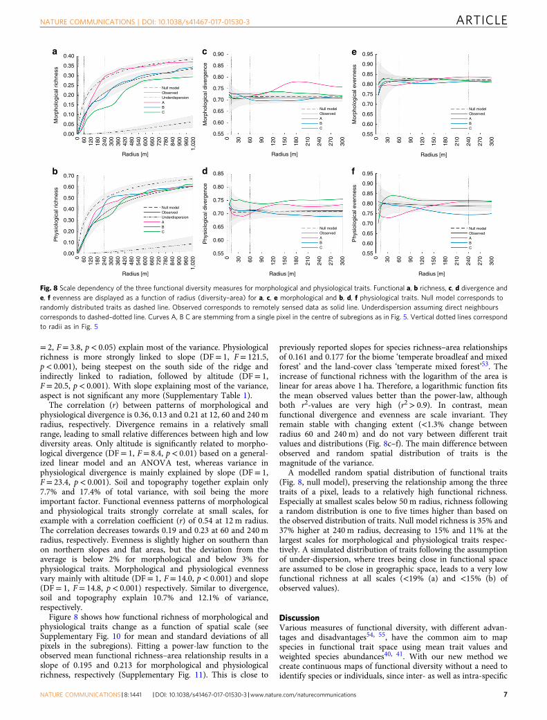
Figure 8 shows how functional richness of morphological andphysiological traits change as a function of spatial scale (seeSupplementary Fig. 10 for mean and standard deviations of allpixels in the subregions). Fitting a power-law function to theobserved mean functional richness–area relationship results in aslope of 0.195 and 0.213 for morphological and physiologicalrichness, respectively (Supplementary Fig. 11). This is close to
previously reported slopes for species richness–area relationshipsof 0.161 and 0.177 for the biome ‘temperate broadleaf and mixedforest’ and the land-cover class ‘temperate mixed forest’53. Theincrease of functional richness with the logarithm of the area islinear for areas above 1 ha. Therefore, a logarithmic function fitsthe mean observed values better than the power-law, althoughboth r2-values are very high (r2> 0.9). In contrast, meanfunctional divergence and evenness are scale invariant. Theyremain stable with changing extent (<1.3% change betweenradius 60 and 240 m) and do not vary between different traitvalues and distributions (Fig. 8c–f). The main difference betweenobserved and random spatial distribution of traits is themagnitude of the variance.
A modelled random spatial distribution of functional traits(Fig. 8, null model), preserving the relationship among the threetraits of a pixel, leads to a relatively high functional richness.Especially at smallest scales below 50 m radius, richness followinga random distribution is one to five times higher than based onthe observed distribution of traits. Null model richness is 35% and37% higher at 240 m radius, decreasing to 15% and 11% at thelargest scales for morphological and physiological traits respec-tively. A simulated distribution of traits following the assumptionof under-dispersion, where trees being close in functional spaceare assumed to be close in geographic space, leads to a very lowfunctional richness at all scales (<19% (a) and <15% (b) ofobserved values).
DiscussionVarious measures of functional diversity, with different advan-tages and disadvantages54, 55, have the common aim to mapspecies in functional trait space using mean trait values andweighted species abundances40, 41. With our new method wecreate continuous maps of functional diversity without a need toidentify species or individuals, since inter- as well as intra-specific
c
d
e
f
0 60 120
180
240
300
360
420
480
540
600
660
720
780
840
900
960
1,02
0
Radius [m]
0.00
0.05
0.10
0.15
0.20
0.25
0.30
0.35
0.40M
orph
olog
ical
ric
hnes
s
Null modelObservedUnderdispersionABC
00
30 60 90 120
150
180
210
240
270
300
Radius [m]
0.55
0.60
0.65
0.70
0.75
0.80
0.85
0.90
Mor
phol
ogic
al d
iver
genc
e
Null modelObservedABC
00
30 60 90 120
150
180
210
240
270
300
Radius [m]
0 60 120
180
240
300
360
420
480
540
600
660
720
780
840
900
960
1,02
0
Radius [m]
30 60 90 120
150
180
210
240
270
300
Radius [m]
30 60 90 120
150
180
210
240
270
300
Radius [m]
0.55
0.60
0.65
0.70
0.75
0.80
0.85
0.90
0.95
Mor
phol
ogic
al e
venn
ess
Null modelObservedABC
0.00
0.10
0.20
0.30
0.40
0.50
0.60
0.70
Phy
siol
ogic
al r
ichn
ess
Null modelObservedUnderdispersionABC
0.55
0.60
0.65
0.70
0.75
0.80
0.85
Phy
siol
ogic
al d
iver
genc
e
Null modelObservedABC
0.55
0.60
0.65
0.70
0.75
0.80
0.85
0.90
0.95
Phy
siol
ogic
al e
venn
ess
Null modelObservedABC
a
b
Fig. 8 Scale dependency of the three functional diversity measures for morphological and physiological traits. Functional a, b richness, c, d divergence ande, f evenness are displayed as a function of radius (diversity–area) for a, c, e morphological and b, d, f physiological traits. Null model corresponds torandomly distributed traits as dashed line. Observed corresponds to remotely sensed data as solid line. Underdispersion assuming direct neighbourscorresponds to dashed–dotted line. Curves A, B C are stemming from a single pixel in the centre of subregions as in Fig. 5. Vertical dotted lines correspondto radii as in Fig. 5
NATURE COMMUNICATIONS | DOI: 10.1038/s41467-017-01530-3 ARTICLE
NATURE COMMUNICATIONS |8: 1441 |DOI: 10.1038/s41467-017-01530-3 |www.nature.com/naturecommunications 7
variability is inherent to remotely sensed functional traits. Espe-cially in relatively species-poor temperate forests, such as the onestudied here, functional diversity might be strongly under-estimated when ignoring intra-specific variability16, 56. Ourmethod avoids this pitfall, because it is fully continuous in spaceand only depends on resolution, it can thus even be applied belowthe individual level. Within-individual variation, for example inleaf traits, is common in plants and can reflect different lightcompetition or leaf ages30. With evolving sensor technologies andminiaturization, higher spectral and spatial resolution of remotelysensed data will allow to study within-individual tree functionaldiversity.
The resulting spatial distribution of morphological and phy-siological diversity generally agree with regard to the spatialpatterns, especially for functional richness. This is related to theenvironmental gradient on the mountain in the observed test areaand the coinciding reduced trait variability towards the ridge(Fig. 4). The mountain ridge is the most prominent landscapefeature of our study area with shallow and rocky soil, steep slopesand high incoming radiation on the south side of the ridge(Supplementary Fig. 5). We can therefore show that both mor-phological and physiological diversity change consistently withtopography and soil. In this case, the abiotic conditions at theridge might act as an environmental filter, only allowing treeswith particular functional traits to exist. This is important becausefunctional richness represents the total extent of the communityniche. The lower functional richness at higher elevation with dry,rocky and shallow soil suggests a smaller range of resourceavailability. Thus smaller biotope space constrained the com-munity niche in this area, which as a consequence may reduce theperformance of the present plant community57 and its adapt-ability to changing environmental conditions40. Therefore, wewould expect the forest communities on the ridge to have lowerecosystem functioning and stability.
Besides similarities in the spatial distribution of functionaldiversity following broad environmental gradients, there are alsoexpected differences between morphological and physiologicaldiversity. These differences are more pronounced for functionaldivergence and evenness than for functional richness. On the onehand, physiological divergence is mainly driven by differencesbetween tree functional groups (needle, broadleaf), because theyhave different leaf structure and composition of pigments andcompounds related to different resource allocation strategies andare therefore clearly divergent in their biochemical characteristics.In areas with mixtures of broadleaf and needle trees, as forexample in subregion C or generally in lower altitudes, pro-ductivity might be increased because the resource use is parti-tioned among the different functional groups leading to lowerresource competition40. At the same time, functional evenness ishigher too, indicating that the niche is filled evenly and availableresources can potentially be fully exploited. In higher altitudeswhere the trait range is reduced, lower divergence and evennesscould mean that there is a stronger competition for resources(nutrients, water) and that some of the resources might be unused,leading to lower productivity and stability of the community.
Morphological diversity, on the other hand, is more stronglylinked to the different stages of forest development (e.g. due todisturbance) and management. For example, subregion A showshigh morphological diversity at larger scales because there is ajuvenile forest patch in the centre surrounded by structurallydifferent mature trees. In contrast, morphological richness,divergence and evenness are low in the managed forest in sub-region C due to equal canopy height and structure. This mayresult in lower productivity due to a lower efficiency in lightcapture, although higher physiological diversity could indicatebetter resource use partitioning among functional groups. The
strong link to the development stage is clearly reflected in themorphological traits themselves. Differences in functional traitsbetween juvenile and mature forest communities can be explainedby changing physiology and morphology with tree age, rangingfrom densely and fast growing highly productive juvenile tomature trees, being characterized by lower growth rate, similarheight, smaller leaves and greater leaf thickness and longevity58.Since the occurrence of patches of juvenile forest is mainly drivenby disturbance and forest management, there is no clear altitu-dinal gradient in functional traits.
In contrast, physiological traits are linked more closely totopographic and soil variables. Equivalent water thickness inparticular shows the strongest altitudinal gradient, because thereis a gradient in soils and steepness leading to lower potentialwater availability towards the top of the ridge. Furthermore,needle trees mainly occurring in lower altitudes show higherEWT and lower relative chlorophyll and carotenoids contentcompared to broadleaf trees. This is in accordance with valuesfrom the TRY database (Supplementary Fig. 7) and a studyconducted at three sites in Switzerland, reporting higher waterand lower nitrogen content, being closely linked to chlorophyllcontent59. In general, our remotely sensed functional traits areconsistent with independent in situ knowledge of the forests inthe study region. We could show that functional traits are map-ped in the correct range and that our measurement values arecompatible with values derived from optical and functional traitdatabases. To map functional diversity, relative trait values can beused but they need to be measured consistently over space. Theproposed remote sensing method has the advantage that it isbased on continuous and consistent large-scale measurementswithout bias due to subjective interpretation or differences inmeasurement techniques or protocols, which can occur whentraits are measured over large areas in the field.
Given the continuous nature of the remotely sensed functionaltrait maps, we were able to study functional diversity at multiplescales and to develop a highly resolved scaling relationship. Therelationship of functional richness and area should be related tothe species–area relationship, which is one of the most studiedecological patterns due to its relevance for predicting biodiversitypatterns and species extinction rates53. Typically, the power-law isused to model species–area relationships resulting in a linearrelationship on the log–log scale. Our results are generally con-sistent between morphological and physiological richness. Fur-thermore, the slope of the relationship on the log–log scale is verysimilar to large-scale species models for temperate mixed for-ests53. However, we also found deviations of the relationship fromthe power-law, as was also reported by Pereira and colleagues forsmaller spatial scales60. Increased within-community diversitywhen considering intra-specific variability might explain thesteeper slope at small scales, whereas species might be redundantwith regard to their functional traits at large scales, leading to aflattening of the log–log relationship. Therefore, we found that alogarithmic function could better predict functional richness thandid the power-law.
Deviations from the average can be observed locally, whenlooking at particular subregions within the test area. Exemplaryfor a steep transition from low to high functional richness withincreasing area is subregion A. Juvenile trees that grow in a dis-turbed area result in low within and high between communitydiversity. In this case, underdispersion at local scale might notonly be driven by abiotic conditions (e.g. environmental filtering)or anthropogenic influence but also by competitive exclusion61.Beech trees might have been planted in disturbed areas orfavoured by environmental conditions, or both, but at the sametime only the fastest growing beech trees with similar functionaltraits might have survived and occupied the new space. When
ARTICLE NATURE COMMUNICATIONS | DOI: 10.1038/s41467-017-01530-3
8 NATURE COMMUNICATIONS | 8: 1441 |DOI: 10.1038/s41467-017-01530-3 |www.nature.com/naturecommunications

competing for light, a competitive ability difference leads to theelimination of individuals that grow slowly and are therefore tooshort to gather enough light61. According to Siefert62, localunder-dispersion leads to locally decreased functional divergenceand increased divergence between environmental patches. This isin agreement with what we observed in subregion A (Fig. 8).
By comparing functional richness–area relationships ofobserved with randomly distributed traits, we found trait con-vergence to be predominant in our forest. However, a general linkbetween community structure and underlying assembly processescan not easily be established, because many processes can lead totrait divergence or convergence, including anthropogenic factorsdue to certain management strategies. Opposing processes canbalance each other and not be disentangled any more44, 63, 64. Thelatter might be the case when looking at the average signal offunctional divergence and evenness, which is scale invariant andalmost similar to the null model. This, however, does not meanthat there is no spatial variation of these two aspects of diversityat all. To study the scale dependency of biodiversity, it is thereforecrucial to not only focus on general relationships but also onspatially continuous diversity patterns at different scales.
In conclusion, combined airborne imaging spectroscopy andlaser scanning allow for mapping functional diversity con-tinuously across large areas of forest using a trait-based, pixel-level approach. We evaluated the diversity of six key traits at avariety of spatial scales and were able to validate these mea-surements against in situ data, as well as to assess communitystructure across an entire landscape. By concentrating on func-tional traits at a continuous spatial resolution without reference tospecies identities or individuals, we were able to include intra-specific variability, which is crucial to assess functional diversityof temperate forests and often neglected when functional diversityis indirectly calculated from taxonomic data. Future studies canadvance the integration of remotely sensed functional data withdatabases of plant functional traits, environmental and ecosystemdata, and dynamic vegetation models to increase our under-standing of the mechanistic linkages between functional diversityand ecosystem function.
To map functional diversity from space and predict globalpatterns of ecosystem functioning, our method could also beapplied to satellite measurements, even though at lower spatialresolution. To test the scalability of our approach we suggestlooking at changing extent and grain in a combined fashion.Supplementary Figure 12 indicates how well richness patternscorrelate at a given neighbourhood radius when changing grain aspixel size. For example, satellite data at 30 m spatial resolutionmight be able to capture richness patterns at 200 m radius with acorrelation coefficient of 0.7–0.8. This paves the way for possiblelarge-scale applications, but further research is needed to quantifyhow much small-scale variability would be lost when pixel size isincreased, and how this would affect diversity–productivityrelationships.
MethodsStudy area. The study area is a temperate mixed forest at the Laegern mountain inSwitzerland (47° 28′43.0 N, 8° 21′53.2 E). The Laegern is characterized by amountain ridge spanning in east–west direction with an altitudinal gradient of450–860 m above sea level (Fig. 1). The extent of the study area is ∼2 km × 6 km. InDecember 1999, the Laegern mountain was affected by a winter storm. The westernpart of the temperate forest was severely hit, resulting in disturbance areas filling inwith beech trees as new stands are initiated. Since forest clear cuts are limited to amaximum area of 0.5 ha, larger patches of juvenile trees likely exist due to thestorm. In 2010, the juvenile trees were 10–15 m high and growing in dense patcheswith a growth rate of around one metre per year65. The mainly closed canopyconsists of a total of 13 species and seven canopy structure types, from single- tomulti-layered canopies66. Roughly 70% of the total forested area is covered bydeciduous broadleaf trees, whereas the remaining 30% of the area is covered byevergreen coniferous trees (forest inventory data). The dominating deciduous
species are common beech (Fagus sylvatica), European ash (Fraxinus excelsior) andsycamore maple (Acer pseudoplatanus). The dominating coniferous species areNorway spruce (Picea abies) and silver fir (Abies alba). Most of the conifers atLaegern were introduced anthropogenically. Naturally, the whole Laegern forestwould be dominated by different hilly to submontane beech communities with fewscattered coniferous needle trees. There are mature trees up to 165 years of age,150 cm of diameter and canopies up to 55 m of height. The study area comprises areference site for forest ecosystem research with an extensive set of ground mea-surements36, 66.
Airborne remote sensing data. The data of the Laegern study area was acquiredin 2010 using airborne laser scanning based on the principle of light detection andranging (LiDAR) and airborne imaging spectroscopy. The LiDAR acquisition wasflown on 1 August 2010 using a helicopter-based scanner system with a rotatingmirror (RIEGL LMS-Q680i, scan angle ±15°). The campaign was flown under leaf-on conditions with a nominal height of 500 m above ground, resulting in a foot-print size of 0.25 m and an average point density of 40 pts/m2. The 3D point cloudwas extracted from the full waveforms of individual laser pulses using Gaussiandecomposition. The LiDAR data was registered to the Swiss national grid CH1903+with a positional accuracy of <0.15 m in vertical and <0.5 m in horizontaldirection.
Imaging spectroscopy acquisitions were flown on 26 June and 29 June 2010under clear sky conditions using the APEX imaging spectrometer34. The study areawas covered with three flight lines on each of the acquisition dates. The averageflight altitude was 4,500 m a.s.l. resulting in an average ground pixel size of 2 m.APEX measured at-sensor radiances in 316 spectral bands ranging from 372 nm to2,540 nm. APEX data were processed to hemispherical-conical reflectance factorsin the APEX Processing and Archiving Facility67. Processing started with the rawinstrument data, which was split into image, dark current and housekeeping data,thus forming level 0. Level 1 (L1) calibrated radiances were obtained by invertingthe instrument model, applying coefficients established during calibration andcharacterization at the APEX Calibration Home Base68. The position andorientation of each pixel in 3D space was based on automatic geocoding in PARGEv3.269, using the swissALTI3D digital terrain model. L1 data were then convertedto HCRF by employing ATCOR4 v7.0 in the smile aware mode. This essentiallyaccounts for the spectral response function of each individual pixels of thespectrometer to reduce biases due to spectral shifts34.
Environmental data. Stand polygons of Kanton Aargau and Zurich include foreststand information on development stage, the percentage coverage of the six mostdominant species, and the percentage coverage of deciduous broadleaf and con-iferous needle trees. The data from Kanton Aargau was provided by AargauischesGeografisches Informationssystem (AGIS), Departement Bau, Verkehr undUmwelt, Abteilung Wald (last updated on 27 February 2015). The data fromKanton Zurich was provided by Geographisches Informationssystem (GIS-ZH),Amt für Landschaft und Natur, Abteilung Wald (last updated on 16 September2015). Soil data corresponds to Bodenkarte Baden (Landeskarte der Schweiz 1:25′000, Blatt 1070), provided by Eidgenössische Forschungsanstalt für Agrarökologieund Landbau (FAL).
Topographic variables (altitude, slope, aspect, curvature) were calculated basedon the digital terrain model derived from a LiDAR acquisition on 10 April underleaf-off conditions. The campaign was flown with a nominal height of 500 m aboveground, resulting in a footprint size of 0.25 m and an average point density of 20pts/m2. Radiation was simulated as incoming photosynthetically active radiation atthe top of canopy (see Supplementary Note 1 for details). Supplementary Fig. 13shows a comparison between simulated and measured radiation at the fluxtower inthe Laegern forest.
Field data. At the Laegern reference site, field survey was conducted on an area of∼5.5 ha to map the exact ground location and taxonomic identity of all dominantand co-dominant trees (1,307 trees with dbh >20 cm). The positions measured onthe ground were linked to a detailed crown map derived from high-resolutiondrone images. Leaf optical properties of sunlit leaves were measured for ten Acerpseudoplatanus, Fraxinus excelsior, Fagus sylvatica, Ulmus glabra and Tilia platy-phyllos trees in June 2009 and for 50 Fagus sylvatica trees in July 2016. For the 50trees, SPAD measurements were taken of the same leaves. Leaf optical propertiesand lab measured traits (chlorophyll, carotenoids, EWT) of 168 Acer pseudopla-tanus trees were used from the ANGERS spectral database.
Functional traits. Functional traits were measured and mapped using state-of-the-art airborne remote sensing methods. A set of three morphological and threephysiological traits was selected and mapped based on airborne laser scanning andimaging spectroscopy data respectively. The whole work-flow from remote sensingdata to functional diversity measures is illustrated in Supplementary Fig. 14.
We selected CH, PAI and FHD as the three main morphological traits, being ofhigh ecological relevance and measurable using airborne laser scanning methods.CH was measured as the distance between the highest laser return from the canopyand the corresponding ground point following Schneider et al.36. PAI was retrievedas the projected surface area of plant material per unit ground area. This includes
NATURE COMMUNICATIONS | DOI: 10.1038/s41467-017-01530-3 ARTICLE
NATURE COMMUNICATIONS |8: 1441 |DOI: 10.1038/s41467-017-01530-3 |www.nature.com/naturecommunications 9
woody as well as foliar material, since laser returns from twigs or leaves can not bedistinguished. PAI was derived from the LiDAR point cloud data on a 2 × 2 mgrid36, 65. FHD is a measure of canopy layering and has been recognized as a majorfunctional trait for characterizing biodiversity of a variety of species and habitats70.FHD was calculated by applying the Shannon–Wiener diversity index on verticalPAI profiles as described by MacArthur and MacArthur71:
FHD ¼ �X
i
pi � logepi; ð1Þ
where pi is the proportion of the total foliage which lies in the ith canopy layer.FHD is a combined measure of how different the layers are with respect to layerdensity (PAI) and how many layers there are in total. Therefore, a certaincorrelation to CH can be expected, since the maximum possible number of layers isgiven by the canopy depth in conjunction with the vertical resolution of the lasersystem. The three morphological traits were normalized to values between 0 and 1and resampled to 6 × 6m spatial resolution using bilinear interpolation,approximating the average basal crown area of the Laegern forest.
Gitelson et al.72 developed a band specific model to derive CHL and CAR fromimaging spectroscopy data in relative units. It has been applied to a wide range ofecosystems, from crops to grasslands and forests38, 73. To derive CHL and CARusing the three-band model72, the following band combinations were used:
CHL ¼ 1R540�560
� 1R760�800
� �� R760�800; ð2Þ
CAR ¼ 1R510�520
� 1R690�710
� �� R760�800; ð3Þ
where Ri−j is the mean reflectance in the spectral range of i to j nanometre. Themodel includes anthocyanins as a third pigment72. We decided not to include it inour study, since anthocyanins can mainly be observed during leaf development orleaf senescence38. Concentrations are generally low during the summer monthsand are difficult to detect, since the absorption features are strongly overlappingwith chlorophyll and carotenoids absorption.
As a third physiological trait, we included EWT. We estimated relative EWTwith a simple ratio water content index based on Underwood et al.74:
EWT ¼ 1� R1;193
R1;126; ð4Þ
where Ri is the reflectance at i nanometre.To reduce the effects of shadows in the traits retrieval, we combined two
airborne imaging spectroscopy acquisitions flown at different times of the day andaggregated 3 × 3 pixels to 6 × 6 m resolution trait data by averaging the threebrightest pixels. To fuse the flight lines, we performed an additional geometrical co-registration using scale-invariant feature transform and random sample consensusalgorithms of the VLFeat package (VLFeat, sift_mosaic, Matlab). Finally, wenormalized to values between 0 and 1.
Estimating physiological forest traits from airborne observations is achallenging task due to the difficulty of linking leaf and canopy level biochemistry.Airborne imaging spectroscopy measures a spatially integrated signal of the sunlitupper canopy of the forest. The mapping of functional diversity relies on relativetrait values being derived from these consistent radiometric measurements. Therelationship of relative trait values and their physical counterparts can bedemonstrated by parametrizing the radiometric simulation of selected species withfield data and generic data from two functional trait databases. The ranges ofphysiological traits were compared with modelled trait ranges based on the leafoptical properties measured in the field in July 2009 (Supplementary Fig. 6). Thesame modelling framework as in ref. 36 was used to simulate canopy reflectancespectra and subsequently derive physiological traits. Constant optical properties forbroadleaf and needle trees were expected to result in a narrower trait range due tothe lack of intra- and inter-specific trait variability within functional groups. Forfurther details on the modelling approach, see Supplementary Note 2.
Field data of the 5.5 ha area at Laegern was used to calculate community-weighted mean chlorophyll and EWT. Species abundances and mean traits werecalculated per 30 × 30 m plot. Remotely sensed mean trait values were thencompared to community-weighted means of the functional trait database TRY29,based on the plot-level species abundances and species-level trait values from TRY(Supplementary Fig. 7). There were not enough measurements in the TRY databaseto calculate community-weighted means of carotenoids.
To illustrate the scalability of the spectral indices from the leaf to the canopylevel, we used the field data to simulate canopy reflectances for the 518 Fagussylvatica and the 168 Acer pseudoplatanus trees on the 5.5 ha area. We used the leafoptical properties of 50 Fagus sylvatica trees measured in July 2016, and randomlydistributed them over the 518 Fagus sylvatica trees according to field survey.Chlorophyll values were then derived from the reflectance spectra at leaf andcanopy level, to be compared to the SPAD measurements of the same leaves(Supplementary Fig. 8). Additionally, we simulated canopy spectra for the 168 Acerpseudoplatanus trees with leaf optical properties of the ANGERS database. Labmeasurements of chlorophyll, carotenoids and EWT from the database were then
compared to traits estimated using spectral indices at leaf and canopy level(Supplementary Fig. 9). Since we did not expect very high carotenoidsconcentrations at Laegern in summer, we fitted a second linear regression inSupplementary Fig. 9c, d for values below 15 μg/m2. For further details on themodelling approach, see Supplementary Note 2.
For mapping in Fig. 3, we used red, green and blue (RGB) colour composites ofthe three normalized morphological and physiological traits respectively. We defineblue areas in the morphological trait map as values of CH<0.5, FHD<0.5 andPAI>0.5, pink areas as CH>0.5, FHD>0.5 and PAI>0.5, and green areas asCH<0.5, FHD>0.3, PAI<0.5. A small area appearing yellow is defined by CH>0.7,FHD>0.7 and PAI<0.6. In the physiological trait map, we define blue areas asvalues of CHL<0.5, CAR<0.5 and EWT>0.5, bright green areas as CHL>0.8,CAR>0.5 and EWT<0.5, and green areas as CHL>0.5, CAR<0.5 and EWT<0.5.Orange areas are characterized by CHL<0.7, CAR>0.7 and EWT<0.5.
The forested area was determined based on CH. To derive the forest mask, wefirst applied a threshold of 10 m CH to select the mature forest pixels and removepossible agricultural fields. We then filled the gaps within the forest to includejuvenile forest patches again. Finally, a threshold of 4 m CH was applied to removegaps and understorey vegetation. We defined a tree to be four or more metres high,as was done in Schneider et al.36 to separate understorey and the canopy.
Functional diversity. Having tens to hundreds of thousands of pixels to map iscomputationally demanding, guiding our choice of index. As a consequence, weselected functional richness, divergence and evenness being computationallymanageable and relatively easy to interpret, since different aspects of functionaldiversity are covered by separate indices. The indices for functional richness,divergence and evenness were calculated based on the remote sensing derivedphysiological and morphological traits. We mapped pixels within a certain radialneighbourhood in the functional trait space, using a moving window approach withvarying neighbourhoods to cover the whole study area. Figure 2 shows an exampleof functional richness, evenness and divergence calculated based on pixels in aradius of 120 m mapped in trait space. Abundance weighting is not needed sinceevery pixel represents a set of trait measurements, not averaged by communities orspecies. With continuous area-based data, however, a single pixel does notnecessarily cover an individual crown. Contributions of more than one individualor species to the functional traits of a singular pixel is possible and thereforerepresents no direct link to species. Detailed information on the three indices andpixel based application is given in the following paragraphs.
Functional richness is a measure of niche extent, where niche is the functionalspace occupied by a species, community or assemblage of trees. It was calculated bymapping pixels of a certain neighbourhood in functional space, whose axes aredefined by the functional traits. Richness was then calculated as the convex hullvolume of the mapped pixels (convhull, Matlab). Supplementary Figure 15 illustratesan artificial example of an increasing functional richness from 0.17 to 0.31.
Since we assign equal weighting to all pixels (no abundances), we calculateddivergence (FDiv) based on Villéger et al.41 as follows:
Δjdj ¼XS
i¼1
1S� jdGi � dGj; ð5Þ
FDiv ¼ dG
Δjdj þ dG; ð6Þ
where S is the number of pixels mapped in the functional space, dGi is theEuclidean distance between the ith pixel and the centre of gravity and dG is themean distance of all pixels to the centre of gravity. In this specific case, a functionaldivergence of 1 would mean that all pixels lie on a sphere with equal distance to thecentre of gravity (Supplementary Fig. 15).
The functional evenness index (FEve) was calculated based on the minimumspanning tree (Fig. 2). A distance matrix with Euclidean distances between all thepoints in the functional space was the basis for deriving the minimum spanningtree using the algorithm of Prim75 (graphminspantree, Matlab). Finally, evennesswas calculated following Villéger et al.41:
PEWl ¼ EWl
PS�1
l¼1EWl
; ð7Þ
FEve ¼PS�1
l¼1min PEWl ;
1S�1
� �� 1S�1
1� 1S�1
;ð8Þ
where EWl is the Euclidean distance of branch l in the minimum spanning tree,PEW is the partial weighted evenness and S is the number of pixels mapped in thefunctional space. Thus S−1 corresponds to the number of branches in theminimum spanning tree. A weighting by species abundance is not necessary whenmapping pixels, since abundance is inherent in the data (Supplementary Fig. 15).
ARTICLE NATURE COMMUNICATIONS | DOI: 10.1038/s41467-017-01530-3
10 NATURE COMMUNICATIONS | 8: 1441 |DOI: 10.1038/s41467-017-01530-3 |www.nature.com/naturecommunications

Scaling. To calculate the functional diversity indices for the whole forest, we used amoving window approach (Supplementary Fig. 16). This means that the indexvalues were calculated for each pixel by iterating through all pixels of the functionaltrait maps. Since diversity is always measured within a certain geographical unit,we used a radial neighbourhood of pixels to calculate the indices. Therefore, theinitial pixel size of 6 × 6 m of the functional trait maps corresponds to the grain,whereas the neighbourhood of pixels corresponds to the extent (SupplementaryFig. 16). We calculated the diversity indices for an increasing neighbourhood of6–1,020 m radius with steps of 6 m, resulting in an extent ranging from 113 to3.27×106 m2. To derive diversity–area curves, we averaged the index values of allforested pixels for each of the 170 extents. For display in Figs. 5–7 and visualassessment, we applied a circular averaging filter (fspecial, disk, Matlab).
Null models. We created a null model of randomly distributed trees, or here pixels,to test if the functional traits distribution follows a random distribution, over- orunder-dispersion. For each tree or pixel, we kept the traits relationship among thethree morphological and physiological traits constant. We then reshuffled thepixels to create random distribution in geographic space (rand, Matlab). Opposedto randomly distribute each trait individually, the trait relationships still hold in thenull model. However, there is no spatial autocorrelation any more.
A second null model is used to simulate maximal under-dispersion, whichcould be resulting from maximal environmental filtering. In this case, we assumethat neighbouring pixels in geographic space are also neighbours in functional traitspace. For each pixel, it is not the neighbouring pixels in a certain radius which areused to calculate the diversity indices. Instead, the same number of neighbouringpixels are selected from the trait space according to minimal Euclidean distance.This results in a purely theoretical null model, where closest neighbours ingeographic space would be closest neighbours in trait space.
Statistical analysis. We tested whether patterns of functional traits and traitdiversity can be explained by abiotic factors related to topography, soil andradiation (see Supplementary Fig. 4 and Supplementary Table 1). To account forspatial autocorrelation, we used a spatially simultaneous autoregressive error modelestimation based on first order neighbours (R package spdep, errorsarlm76) to fit ageneralized linear model.
Subsequent analysis of variance (ANOVA) with type-I sum of squares wasperformed at 60 m radius scale. The forest was sampled using 467 pixels projectedon a regular grid such that their circular neighbourhood areas did not overlap andremained fully within forest boundaries. Continuous explanatory variables wereaveraged within 60 m radius, whereas simple majority was used for categoricalvariables. Continuous explanatory variables were altitude, slope, soil depth andamount of rocky materials. The categorical variable aspect was subdivided in threecategories, namely north, south and flat slopes. Curvature was grouped incategories valley, ridge and flat areas. Soil type consisted of eight soil classes(Dystric Cambisols, Luvisols, Endogleyic Cambisols, Stagnic Cambisols, Cambisols,Calcic Cambisols, Leptosols and Regosols, see Supplementary Fig. 5). SupplementaryFigure 4 shows the variance explained based on type-I sum of squares of soil (toppanels) and topography (bottom panels), as well as additionally explained factorswhen adding topography or soil, and radiation to the model. Within groups, theorder of the explanatory variables was kept constant. For Supplementary Table 1,the order of the explanatory variables related to topography were determined bythe significance when tested individually, with the most significant used first in thecombined model.
Data availability. The data that support the findings of this study are availablefrom the corresponding author upon reasonable request. An example of the air-borne laser scanning and imaging spectroscopy data is available at http://www.geo.uzh.ch/microsite/3dveglab/eod/ for a subset of 300 × 300 m. Community and soildata has to be requested directly from the Swiss cantons Zurich or Aargau.
Received: 30 September 2016 Accepted: 25 September 2017
References1. Roscher, C. et al. A functional trait-based approach to understand community
assembly and diversity-productivity relationships over 7 years in experimentalgrasslands. Perspect. Plant Ecol., Evol. Syst. 15, 139–149 (2013).
2. Mouillot, D., Graham, N. A., Villéger, S., Mason, N. W. & Bellwood, D. R. Afunctional approach reveals community responses to disturbances. Trends Ecol.Evol. 28, 167–177 (2013).
3. Calba, S., Maris, V. & Devictor, V. Measuring and explaining large-scaledistribution of functional and phylogenetic diversity in birds: separatingecological drivers from methodological choices. Glob. Ecol. Biogeogr. 23,669–678 (2014).
4. Fründ, J., Dormann, C. F., Holzschuh, A. & Tscharntke, T. Bee diversity effectson pollination depend on functional complementarity and niche shifts. Ecology94, 2042–2054 (2013).
5. Gotelli, N. J. & Colwell, R. K. Quantifying biodiversity: procedures and pitfallsin the measurement and comparison of species richness. Ecol. Lett. 4, 379–391(2001).
6. Violle, C., Reich, P. B., Pacala, S. W., Enquist, B. J. & Kattge, J. The emergenceand promise of functional biogeography. Proc. Natl Acad. Sci. USA 111,13690–13696 (2014).
7. Violle, C. et al. Let the concept of trait be functional! Oikos 116, 882–892(2007).
8. Liu, X. et al. Linking individual-level functional traits to tree growth in asubtropical forest. Ecology 97, 2396–2405 (2016).
9. Sakschewski, B. et al. Resilience of amazon forests emerges from plant traitdiversity. Nat. Clim. Change 6, 1032–1036 (2016).
10. Hooper, D. U. et al. Effects of biodiversity on ecosystem functioning: aconsensus of current knowledge. Ecol. Monogr. 75, 3–35 (2005).
11. Balvanera, P. et al. Quantifying the evidence for biodiversity effects onecosystem functioning and services. Ecol. Lett. 9, 1146–1156 (2006).
12. Cardinale, B. J. et al. The functional role of producer diversity in ecosystems.Am. J. Bot. 98, 572–592 (2011).
13. Barrufol, M. et al. Biodiversity promotes tree growth during succession insubtropical forest. PLoS ONE 8, e81246 (2013).
14. Liang, J. et al. Positive biodiversity-productivity relationship predominant inglobal forests. Science 354, aaf8957 1–12 (2016).
15. Hillebrand, H., Bennett, D. M. & Cadotte, M. W. Consequences of dominance:a review of evenness effects on local and regional ecosystem processes. Ecology89, 1510–1520 (2008).
16. Cadotte, M. W., Carscadden, K. & Mirotchnick, N. Beyond species: functionaldiversity and the maintenance of ecological processes and services. J. Appl. Ecol.48, 1079–1087 (2011).
17. Zhang, Y., Chen, H. Y. H. & Reich, P. B. Forest productivity increases withevenness, species richness and trait variation: a global meta-analysis. J. Ecol.100, 742–749 (2012).
18. Williams, L. J., Paquette, A., Cavender-Bares, J., Messier, C. & Reich, P. B.Spatial complementarity in tree crowns explains overyielding in speciesmixtures. Nat. Ecol. Evol. 1, 63 (2017).
19. Chamagne, J. et al. Forest diversity promotes individual tree growth in centraleuropean forest stands. J. Appl. Ecol. 54, 71–79 (2017).
20. Ruiz-Benito, P. et al. Functional diversity underlies demographic responses toenvironmental variation in european forests. Glob. Ecol. Biogeogr. 26, 128–141(2017).
21. McGill, B. J., Enquist, B. J., Weiher, E. & Westoby, M. Rebuilding communityecology from functional traits. Trends Ecol. Evol. 21, 178–185 (2006).
22. Cianciaruso, M. V., Batalha, M. A., Gaston, K. J. & Petchey, O. L. Includingintraspecific variability in functional diversity. Ecology 90, 81–89 (2009).
23. Petchey, O. L. & Gaston, K. J. Functional diversity (fd), species richness andcommunity composition. Ecol. Lett. 5, 402–411 (2002).
24. Laughlin, D. C., Joshi, C., van Bodegom, P. M., Bastow, Z. A. & Fulé, P. Z. Apredictive model of community assembly that incorporates intraspecific traitvariation. Ecol. Lett. 15, 1291–1299 (2012).
25. Luo, Y.-H. et al. Trait-based community assembly along an elevational gradientin subalpine forests: quantifying the roles of environmental factors in inter- andintraspecific variability. PLoS ONE 11, 1–20 (2016).
26. Ferretti, M. & Fischer, R. Forest Monitoring: Methods for TerrestrialInvestigations in Europe with an Overview of North America and Asia, vol. 12 ofDevelopments in Environmental Science (UK, Elsevier Science, 2013).
27. Bussotti, F., Pollastrini, M., Holland, V. & Brüggemann, W. Functional traitsand adaptive capacity of European forests to climate change. Environ. Exp. Bot.111, 91–113 (2015).
28. Pérez-Harguindeguy, N. et al. New handbook for standardised measurement ofplant functional traits worldwide. Aust. J. Bot. 61, 167–234 (2013).
29. Kattge, J. et al. TRY-a global database of plant traits. Glob. Change Biol. 17,2905–2935 (2011).
30. Li, X., Pei, K., Kéry, M., Niklaus, P. A. & Schmid, B. Decomposing functionaltrait associations in a chinese subtropical forest. PLoS ONE 12, e0175727 (2017).
31. Jetz, W. et al. Monitoring plant functional diversity from space. Nat. Plants 2,1–5 (2016).
32. Gray, A. Monitoring stand structure in mature coastal douglas-fir forests: effectof plot size. For. Ecol. Manag. 175, 1–16 (2003).
33. Homolová, L., Malenovský, Z., Clevers, J. G., García-Santos, G. & Schaepman, M. E.Review of optical-based remote sensing for plant trait mapping. Ecol. Complex. 15,1–16 (2013).
34. Schaepman, M. E. et al. Advanced radiometry measurements and earth scienceapplications with the airborne prism experiment (apex). Remote Sens. Environ.158, 207–219 (2015).
35. Asner, G. P. et al. Airborne laser-guided imaging spectroscopy to map foresttrait diversity and guide conservation. Science 355, 385–389 (2017).
36. Schneider, F. D. et al. Simulating imaging spectrometer data: 3d forest modelingbased on lidar and in situ data. Remote Sens. Environ. 152, 235–250 (2014).
NATURE COMMUNICATIONS | DOI: 10.1038/s41467-017-01530-3 ARTICLE
NATURE COMMUNICATIONS |8: 1441 |DOI: 10.1038/s41467-017-01530-3 |www.nature.com/naturecommunications 11

37. Ishii, H. T., Tanabe, S.-i & Hiura, T. Exploring the relationships among canopystructure, stand productivity, and biodiversity of temperate forest ecosystems.For. Sci. 50, 342–355 (2004).
38. Ustin, S. L. et al. Retrieval of foliar information about plant pigment systemsfrom high resolution spectroscopy. Remote Sens. Environ. 113, S67–S77 (2009).
39. Lawlor, D. W. & Cornic, G. Photosynthetic carbon assimilation and associatedmetabolism in relation to water deficits in higher plants. Plant Cell Environ. 25,275–294 (2002).
40. Mason, N. W. H., Mouillot, D., Lee, W. G. & Wilson, J. B. Functional richness,functional evenness and functional divergence: the primary components offunctional diversity. Oikos 111, 112–118 (2005).
41. Villéger, S., Mason, N. W. H. & Mouillot, D. New multidimensional functionaldiversity indices for a multifaceted framework in functional ecology. Ecology 89,2290–2301 (2008).
42. Salles, J. F., Poly, F., Schmid, B. & Roux, X. L. Community niche predicts thefunctioning of denitrifying bacterial assemblages. Ecology 90, 3324–3332 (2009).
43. Letts, B., Lamb, E. G., Mischkolz, J. M. & Romo, J. T. Litter accumulation drivesgrassland plant community composition and functional diversity via leaf traits.Plant Ecol. 216, 357–370 (2015).
44. van der Plas, F. et al. A new modeling approach estimates the relativeimportance of different community assembly processes. Ecology 96, 1502–1515(2015).
45. Silva Pedro, M., Rammer, W. & Seidl, R. Disentangling the effects of compositionaland structural diversity on forest productivity. J. Veg. Sci. 28, 649–658 (2017).
46. Bohn, F. J. & Huth, A. The importance of forest structure to biodiversity-productivity relationships. R. Soc. Open Sci. 4, 160521 (2017).
47. Forrester, D. I. & Bauhus, J. A review of processes behind diversity-productivityrelationships in forests. Curr. For. Rep. 2, 45–61 (2016).
48. Asner, G. P. et al. Amazonian functional diversity from forest canopy chemicalassembly. Proc. Natl Acad. Sci. USA 111, 5604–5609 (2014).
49. Martin, R. E., Asner, G. P. & Sack, L. Genetic variation in leaf pigment, opticaland photosynthetic function among diverse phenotypes of Metrosiderospolymorpha grown in a common garden. Oecologia 151, 387–400 (2007).
50. Biswas, S. R., Mallik, A. U., Braithwaite, N. T. & Wagner, H. H. A conceptualframework for the spatial analysis of functional trait diversity. Oikos 125,192–200 (2015).
51. Mori, A. S., Furukawa, T. & Sasaki, T. Response diversity determines theresilience of ecosystems to environmental change. Biol. Rev. 88, 349–364 (2013).
52. Karadimou, E. K., Kallimanis, A. S., Tsiripidis, I. & Dimopoulos, P. Functionaldiversity exhibits a diverse relationship with area, even a decreasing one. Sci.Rep. 6, 35420 (2016).
53. Gerstner, K., Dormann, C. F., Václavík, T., Kreft, H. & Seppelt, R. Accountingfor geographical variation in species-area relationships improves the predictionof plant species richness at the global scale. J. Biogeogr. 41, 261–273 (2014).
54. Petchey, O. L. & Gaston, K. J. Functional diversity: back to basics and lookingforward. Ecol. Lett. 9, 741–758 (2006).
55. Mouchet, M. A., Villéger, S., Mason, N. W. H. & Mouillot, D. Functionaldiversity measures: an overview of their redundancy and their ability todiscriminate community assembly rules. Funct. Ecol. 24, 867–876 (2010).
56. Albert, C. H. et al. A multi-trait approach reveals the structure and the relativeimportance of intra- vs. interspecific variability in plant traits. Funct. Ecol. 24,1192–1201 (2010).
57. Dimitrakopoulos, P. G. & Schmid, B. Biodiversity effects increase linearly withbiotope space. Ecol. Lett. 7, 574–583 (2004).
58. Bond, B. J. Age-related changes in photosynthesis of woody plants. TrendsPlant Sci. 5, 349–353 (2000).
59. Huber, S., Kneubühler, M., Psomas, A., Itten, K. & Zimmermann, N. E.Estimating foliar biochemistry from hyperspectral data in mixed forest canopy.For. Ecol. Manag. 256, 491–501 (2008).
60. Pereira, H. M., Borda-de Água, L. & Martins, I. S. Geometry and scale inspecies-area relationships. Nature 482, E3–E4 (2012).
61. Mayfield, M. M. & Levine, J. M. Opposing effects of competitive exclusion onthe phylogenetic structure of communities. Ecol. Lett. 13, 1085–1093 (2010).
62. Siefert, A. Spatial patterns of functional divergence in old-field plantcommunities. Oikos 121, 907–914 (2012).
63. Botta-Dukát, Z. & Czúcz, B. Testing the ability of functional diversity indices todetect trait convergence and divergence using individual-based simulation.Methods Ecol. Evol. 7, 114–126 (2016).
64. Chacón-Labella, J., de la Cruz, M., Pescador, D. S. & Escudero, A. Individualspecies affect plant traits structure in their surroundings: evidence of functionalmechanisms of assembly. Oecologia 180, 975–987 (2016).
65. Schneider, F. D., et al. in Proc. SilviLaser 2015, 14th Conference on LidarApplications for Assessing and Managing Forest Ecosystems (eds Durrieu, S. &Véga, C.) (La Grande Motte, France, 2015).
66. Leiterer, R., Furrer, R., Schaepman, M. E. & Morsdorf, F. Forest canopy-structure characterization: a data-driven approach. For. Ecol. Manag. 358,48–61 (2015).
67. Hueni, A. et al. Structure, components, and interfaces of the airborne prismexperiment (apex) processing and archiving facility. IEEE Trans. Geosci. RemoteSens. 47, 29–43 (2009).
68. Hueni, A., Lenhard, K., Baumgartner, A. & Schaepman, M. E. Airborne prismexperiment calibration information system. IEEE Trans. Geosci. Remote Sens.51, 5169–5180 (2013).
69. Schläpfer, D. & Richter, R. Geo-atmospheric processing of airborne imagingspectrometry data. Part 1: parametric orthorectification. Int. J. Remote Sens. 23,2609–2630 (2002).
70. August, P. V. The role of habitat complexity and heterogeneity in structuringtropical mammal communities. Ecology 64, 1495–1507 (1983).
71. MacArthur, R. & MacArthur, J. On bird species diversity. Ecology 42, 595–599(1961).
72. Gitelson, A. A., Keydan, G. P. & Merzlyak, M. N. Three-band model fornoninvasive estimation of chlorophyll, carotenoids, and anthocyanin contentsin higher plant leaves. Geophys. Res. Lett. 33, 1–5 (2006).
73. Viña, A. Evaluating vegetation indices for assessing productivity along atropical rain forest chronosequence in western amazonia. Israel J. Plant Sci. 60,123–133 (2012).
74. Underwood, E., Ustin, S. & DiPietro, D. Mapping nonnative plants usinghyperspectral imagery. Remote Sens. Environ. 86, 150–161 (2003).
75. Prim, R. C. Shortest connection networks and some generalizations. Bell Syst.Tech. J. 36, 1389–1401 (1957).
76. Bivand, R. & Piras, G. Comparing implementations of estimation methods forspatial econometrics. J. Stat. Softw. 63, 1–36 (2015).
AcknowledgementsThis study has been supported by the University of Zurich Research Priority Program onGlobal Change and Biodiversity (URPP GCB). The research carried out at the Jet Pro-pulsion Lab, California Institute of Technology, was under a contract with the Natio-nalAeronautics and Space Administration. Government sponsorship is acknowledged.Part of the work is based on output from the working group of the National Center forEcological Analysis and Synthesis on ‘Prospects and priorities for satellite monitoring ofglobal terrestrial biodiversity’. Data processing was supported by S3IT (University ofZurich), with assistance of Riccardo Murri and Sergio Maffioletti. We thank CarlaGuillén Escribà, Irene Garonna, Walter Jetz, Reinhard Furrer, Meinrad Abegg and DanielKükenbrink for fruitful discussions on aspects of the manuscript.
Author contributionsF.D.S., F.M., B.S., O.L.P., and M.E.S. designed research; F.D.S., B.S., and M.E.S. per-formed research; F.D.S., F.M., A.H., and M.E.S. analysed data; and F.D.S., F.M., B.S., O.L.P., A.H., D.S.S. and M.E.S. wrote the paper.
Additional informationSupplementary Information accompanies this paper at doi:10.1038/s41467-017-01530-3.
Competing interests: The authors declare no competing financial interests.
Reprints and permission information is available online at http://npg.nature.com/reprintsandpermissions/
Publisher's note: Springer Nature remains neutral with regard to jurisdictional claims inpublished maps and institutional affiliations.
Open Access This article is licensed under a Creative CommonsAttribution 4.0 International License, which permits use, sharing,
adaptation, distribution and reproduction in any medium or format, as long as you giveappropriate credit to the original author(s) and the source, provide a link to the CreativeCommons license, and indicate if changes were made. The images or other third partymaterial in this article are included in the article’s Creative Commons license, unlessindicated otherwise in a credit line to the material. If material is not included in thearticle’s Creative Commons license and your intended use is not permitted by statutoryregulation or exceeds the permitted use, you will need to obtain permission directly fromthe copyright holder. To view a copy of this license, visit http://creativecommons.org/licenses/by/4.0/.
© The Author(s) 2017
ARTICLE NATURE COMMUNICATIONS | DOI: 10.1038/s41467-017-01530-3
12 NATURE COMMUNICATIONS | 8: 1441 |DOI: 10.1038/s41467-017-01530-3 |www.nature.com/naturecommunications