Mapping Environmental Factors for Spatial Epidemiology:

Experiences and Examples

Beat Rihm, Meteotest, Bern

on behalf of the Federal Office for the Environment

(FOEN), Air Pollution Control and Chemicals

Division, Bern

Workshop on epidemiological analysis of air pollution effects on vegetation,

Basel, 16-17 September 2014

Spatial epidemiology: we include environmental factors to study

geographic correlations.

If the explaining/predicting factors (pollutants, climate…) are not

measured at the same site as the dependent ecological factors (growth,

health…) we need "mapping". I.e. we calculate the environmental factors

at the ecological receptor points. Questions arise such as:

• Type of model/interpolation

• Raster vs. sites (points)

• Time vs. space

• Basic parameters

vs. integrated parameters

• Examples:

ammonia,

nitrogen deposition,

ozone flux

Overview

Rihm | page 2

• Point on the earth: xzy, land-use, surface roughness

• Height above ground of measurements.

Reference height of modelled concentrations.

• Forest: above/below canopy, throughfall/open field deposition.

• A line or area: e.g. transects of Swiss Biodiversity-Monitoring

(BDM Z7) in 1x1 km cells:

Plant species observed

along the paths (red).

Deposition was modelled

for points nearby the line

on a hectar-grid (purple).

What Is a Site?

• The differential equations describing atmospheric transport are

calculated numerically.

• Advantages: integrated meteorology and pollutants; long-range

transport; chemical reactions; soil-interaction; prognostic; high

temporal resolution.

• Disadvantages: complex; parametrisation may be difficult; "low"

spatial resolution (mountains, local sources).

• In Switzerland:

- research and case studies at PSI with CAMx

(Sebnem Aksoyoglu et al.).

- model Cosmo 2.2 km at MeteoSwiss, only for meteo (?).

Analytical Atmospheric Models e.g. EMEP Unified

Rihm | page 4

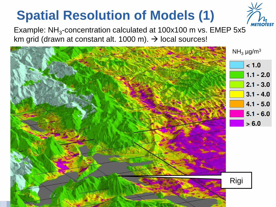
Example: NH3-concentration calculated at 100x100 m vs. EMEP 5x5

km grid (drawn at constant alt. 1000 m). local sources!

Spatial Resolution of Models (1)

Rigi

NH3 µg/m3

Example: NH3 concentration (µg/m3) calculated at 100x100 m and

locations of trees with recorded epiphytic lichens local sources/farms!

Spatial Resolution of Models (2)

• Example: O3-flux spruce, mapped at 250x250 m, EMEP 5 km

grid (drawn at constant alt. 1000 m). Topography/climate!

Spatial Resolution of Models (3)

Jura

Mountains

Swiss

Plateau

Lakes

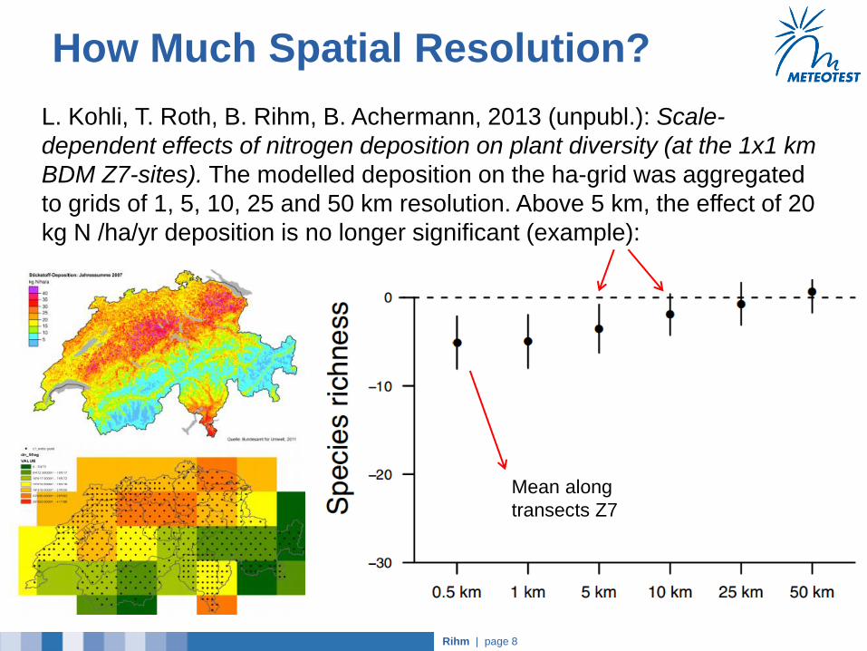
L. Kohli, T. Roth, B. Rihm, B. Achermann, 2013 (unpubl.): Scale-

dependent effects of nitrogen deposition on plant diversity (at the 1x1 km

BDM Z7-sites). The modelled deposition on the ha-grid was aggregated

to grids of 1, 5, 10, 25 and 50 km resolution. Above 5 km, the effect of 20

kg N /ha/yr deposition is no longer significant (example):

How Much Spatial Resolution?

Rihm | page 8

Mean along

transects Z7

Rihm | page 9

1. Climatic parameters such as temp., prec., radiation:

3-D inverse distance model (Shepard’s gravity interpolation), with

vertical scale factors/vertical gradients and local corrections for

northern/southern slopes, cities, lakes, depressions...

http://meteonorm.com/de/downloads/documents (Jan Remund)

2. Primary pollutants closely related to the emission sources:

emission maps and statistical dispersion models:

NH3, NO2, (also SO2, CH4, Benzol, PM10 available).

quality of the emission map is crucial for modeling local peaks.

3. O3 concentration and other integrated parameters (e.g. O3 flux):

geo-statistical interpolation, i.e. regression with available maps of

explaining parameters.

not always feasible, depends on spatial variabilty of the dependent

parameter and the quality of the predictor maps. Spatial

stratification may help.

Mapping Approaches Aiming at High Spatial Resolution

Rihm | page 10

Path ways of reactive N in the atmosphere (Hertel et al. 2011, http://www.nine-esf.org/ENA)

Modeling Nitrogen Deposition with High Spatial Resolution

Geo-statistical interpolation

of monitoring results

Model 100x100 m Model 100x100 m

Rihm | page 11

Ammonia Emission Map, Point Sources (Farms) with ha-Resolution

Example in Jura Mountains:

Raised bog (black dots) with

farms (red class) and crop/

grassland (green class). Forests

are in light blue class.

Circles: 1 and 4 km distance

Rihm | page 12

Methods:

• Dispersion function f(distance), Asman & Jaarsveld (modified)

• Concentration = f(distance) * source_strength

• Deposition = concentration * deposition_velocity

• Ammonia monitoring network with passive samplers (model validation)

Modeling Ammonia Concentration and Deposition

1.0E-09

1.0E-08

1.0E-07

1.0E-06

1.0E-05

1.0E-04

1.0E-03

1.0E-02

1.0E-01

1.0E+00

0 10000 20000 30000 40000 50000

D (m)

land-use type mm s-1

coniferous forest

deciduous forest

agricultural land

surface water

unproductive vegetation

settlement

no vegetation

30

22

12

20

20

8

5

f(distance), distance to source 50m - 50km: Deposition velocities:

Rihm | page 13

Ammonia Landscape: a Sea Urchin

Rihm | page 14

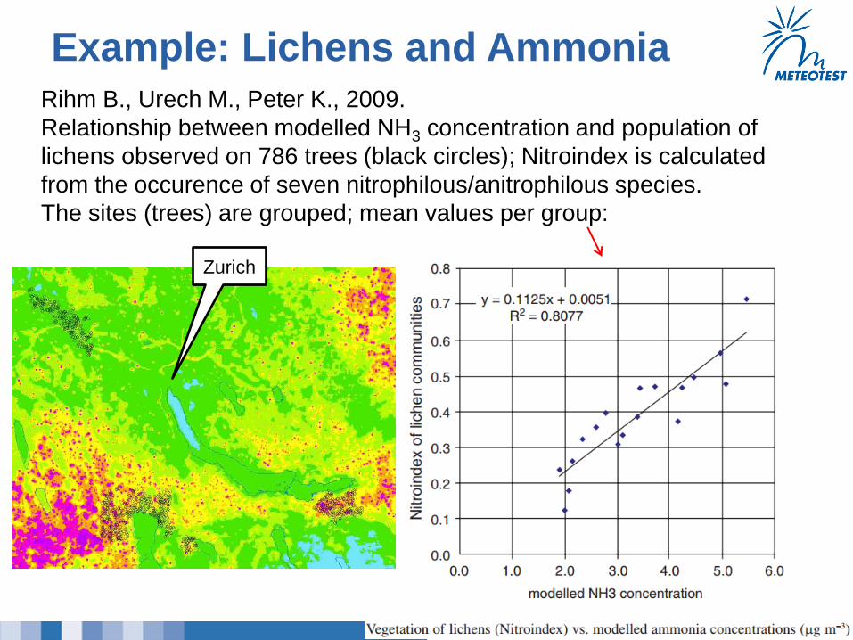
Rihm B., Urech M., Peter K., 2009.

Relationship between modelled NH3 concentration and population of

lichens observed on 786 trees (black circles); Nitroindex is calculated

from the occurence of seven nitrophilous/anitrophilous species.

The sites (trees) are grouped; mean values per group:

Example: Lichens and Ammonia

Zurich

Rihm | page 15

Braun S./IAP 2004: Relationship between N-deposition and the

occurence of blackberries in forest observation plots.

Example: N and Blackberries

Rihm and Braun | page 16 | January 28, 2014

• Selection of 38 monitoring stations for ozone and meteorology.

Mapping Ozone Flux (POD1) with High Spatial Resolution, 1991-2011

Rihm | page 17

• The O3 concentration is highly variable in time and space as

shown during this 1-day-episode in the region of Basel (output of

the analytical model Berphomod, 1998; animated gif).

Problem: Hourly O3 Concentration for POD1 Calculation (1)

Rihm | page 18

• Hourly O3 concentration maps derived from monitoring stations

are produced for public information, but they are too coarse for

site-specific POD1 calculations

http://www.bafu.admin.ch/luft/luftbelastung/blick_zurueck/04751/in

dex.html?lang=en

• Idea: Calculate POD1 at the 39 monitoring stations (where hourly

O3 and meteo values are available) and then try to map that

integrated parameter, instead of the "basic" O3 concentration.

Problem: Hourly O3 Concentration for POD1 Calculation (2)

POD1 1991-2011, DO3SE, 38 Stations Station 1991 1992 1993 1994 1995 1996 1997 1998 1999 2000 2001 2002 2003 2004 2005 2006 2007 2008 2009 2010 2011 MEAN

AIG 12 6 11 5 8

ANI 14 14 9 14 11 12

ARO 6 6 5 8 5 4 4 6 5 7 6 4 14 6 7 10 11 12 13 11 12 8

BAC 21 23 23 20 20 21 20 20 21 20 20 21 19 19 19 20 20

BAS 14 14 13 13 15 15 15 17 17 17 6 17 10 14 17 16 16 15 15 15 13 14

BRU 20 21 22 20 18 20

CAS 17 17 17 18 15 17

CHA 24 25 22 24 23 24 27 26 28 26 26 26 25 26 25 24 22 23 24 22 23 25

chablais 14 14 14 18 17 11 19 17 19 16 8 13 11 13 14

DAV 13 15 13 15 13 14 15 14 15 14 14 15 16 15 14 14 13 13 14 12 12 14

DOR 23 26 32 24 17 39 10 21 18 17 5 17 11 17 17 16 11 12 10 10 10 17

DUE 11 13 13 13 15 16 15 16 15 13 14 15 11 16 15 14 15 15 15 14 14 14

EGG 15 12 8 13 4 10

ETZ 17 18 19 12 17 14 14 19 18 18 19 16 17

GIE 12 16 16 18 14 15

LAE 14 16 15 15 15 16 16 16 18 18 17 18 10 19 17 16 16 16 17 15 15 16

LLA 20 17 15 12 16

MAG 12 13 16 12 16 18 15 17 17 16 14 16 13 14 15 14 13 15 13 14 14 15

muri 12 17 13 16 15 13 11 18 16 15 14 13 14 11 9 14

PAS 16 15 11 15 11 14

PAY 23 22 21 21 21 22 23 16 25 13 24 25 16 23 23 22 19 18 12 16 13 20

RIG 24 25 22 25 23 23 25 25 26 26 25 24 27 25 24 25 21 22 22 20 23 24

sagno 29 34 37 22 29 35 25 22 24 24 21 23 21 17 24 26

SAI 21 22 20 21 19 21

schoebu 22 25 21 24 23 18 22 16 12 11 16 7 10 12 12 13 12 14 16 12 16

sciss 30 24 23 24 27 16 24 18 19 11 17 21

SGS 22 19 15 16 16 12 20 22 21 25 22 23 24 25 24 22 20 19 20 20 23 20

SIS 10 11 13 12 15 15 17 13 15 16 15 17 9 14 15 14 15 14 16 15 11 14

SOG 17 17 18 17 16 17

STA 26 41 38 35 23 22 32 25 30

STM 13 14 13 14 14 14 15 15 15 13 13 14 14 12 12 11 11 13 11 11 13

SYZ 11 12 11 11 13 11

TAE 18 18 18 18 19 20 21 22 20 21 20 20 18 21 19 18 19 19 19 17 19 19

TUR 11 7 5 9 4 7

WEE 20 19 20 16 12 17

wengen 15 18 12 11 11 15 13 12 14 7 10 10 7 8 12

WLD 21 19 20 20

ZIM 21 23 25 23 21 23

zugerb 22 25 26 22 26 29 18 23 23 25 21 17 19 13 21 22

n 13 16 17 17 17 17 20 22 23 24 24 24 23 24 24 24 33 36 35 36 35 24

Rihm | page 19

(Beech)

Scheme POD1 Mapping

Forest Sites

F1..F4:

Tree Growth,

4-yr-means

Soil water Epidemiological

Analysis

Spatial interpolation of POD1, 1991-2011

F1 F2 F3 F4

Air Monitoring

Sites A1..A5:

Ozone, Meteo:

hourly data for

DO3SE model

(POD1)

Temporal

resolution

1 year

Beech, POD1 mean 1991-2011 (mmol/m2/yr): (spruce not shown)

POD1 = -33.01 + 0.4984 * relh + 0.2093 * (o3mean0.333 * zq)

adj.R2 = 0.51, n = 38, units: mmol m-2 yr-1

Predictor maps, 250 m raster:

1) zq = -11.59 * z2 + 23.61 * z + 7.40 , z = altitude (km)

2) o3mean: mean ozone concentration (µg m-3), 1996-1998

3) relh: relative air humidity (%)

Geo-statistical Interpolation Using Predictor Maps & Regression Analysis

y = -0.00001159x2 + 0.02361352x + 7.40055626R² = 0.33118291

0.000

5.000

10.000

15.000

20.000

25.000

30.000

0 500 1000 1500 2000

z

z

Poly. (z)

POD1 Beech, Mean 1991-2011

Rihm | page 23

The spatial pattern of the POD1 average 1991-2011 is quite stable; the

chosen input-maps explained 51% of the variation.

For the epidemiological analysis the temporal resolution is crucial as

the stem growth relative to the average stem growth is analysed.

We need yearly maps. Is there an easy way for calculating them?

Look at relative flux: relPOD1year = POD1year / POD1991-2011

relPOD1 of all stations is ~linear! Mean R2 1991-2011 = 0.78

POD1, Yearly Maps 1991-2011 (1)

y = 1.2096x - 4.6302R² = 0.8518

0.00

5.00

10.00

15.00

20.00

25.00

30.00

0.00 5.00 10.00 15.00 20.00 25.00

BD1SW_2011

BD1SW_2011

Linear (BD1SW_2011)

y = 0.8789x + 2.4013R² = 0.857

0.00

5.00

10.00

15.00

20.00

25.00

0.00 5.00 10.00 15.00 20.00 25.00

BD1SW_2007

BD1SW_2007

Linear (BD1SW_2007)

Rihm | page 24

As relPOD1 behaves quite linearly, we can map it with a inverse-distance

weight (IDW) interpolation: no further data are needed.

The yearly POD1 maps are calculated by multiplying the relPOD1-map

with the POD1 average map on a cell-by-cell basis;

examples 2007 and 2011:

POD1, Yearly Maps 1991-2011 (2)

Rihm | page 25

1) If the sites are influenced by local sources of pollutants (e.g. NH3),

the spatial resolution of the model should depict the horizontal

gradients around those sources (cellsize ~ 0.1 – 0.5 km).

For secondary pollutants (e.g. O3) larger cellsizes may be OK.

2) If topography around sites is complex, meteo parameters show

strong gradients.

For depicting alpine valleys: cellsize < 0.5 – 2 km

3) For spatial epidemiology we need gradients in the environmental

factors. The mapping of these factors must have enough spatial

resolution to depict the gradients within the investigation area.

4) Sub-grid variation of factors leads to scatter or also to bias (if the

sites are not randomly situated).

Comments and Conclusions - Spatial Resolution

Rihm | page 26

5) If analytical atmospheric models cannot be applied (costs, complexity,

spatial resolution) geo-statistical interpolation and statistical

dispersion models might be useful.

6) For defined investigation areas, the spatial pattern of environmental

factors is often easier to be mapped if the factors are time-averaged

or integrated.

7) For mapping environmental factors, clarify what is essential in the

epidemiological analyis: variation in time or in space. Mapping is

generally easier if not both, time and space, must be in high

resolution.

8) Avoid using unnecessary "bad" data in the mapping process, i.e.

input maps with small predicting power in comparison with their

quality.

Comments and Conclusions - Mapping Methods

Thank you for your attention!

Beat Rihm, Meteotest

Churfirsten in clouds (CH)