warwick.ac.uk/lib-publications

Manuscript version: Author’s Accepted Manuscript The version presented in WRAP is the author’s accepted manuscript and may differ from the published version or Version of Record. Persistent WRAP URL: http://wrap.warwick.ac.uk/92780 How to cite: Please refer to published version for the most recent bibliographic citation information. If a published version is known of, the repository item page linked to above, will contain details on accessing it. Copyright and reuse: The Warwick Research Archive Portal (WRAP) makes this work by researchers of the University of Warwick available open access under the following conditions. Copyright © and all moral rights to the version of the paper presented here belong to the individual author(s) and/or other copyright owners. To the extent reasonable and practicable the material made available in WRAP has been checked for eligibility before being made available. Copies of full items can be used for personal research or study, educational, or not-for-profit purposes without prior permission or charge. Provided that the authors, title and full bibliographic details are credited, a hyperlink and/or URL is given for the original metadata page and the content is not changed in any way. Publisher’s statement: Please refer to the repository item page, publisher’s statement section, for further information. For more information, please contact the WRAP Team at: wrap@warwick.ac.uk.

Discrete Longitudinal Data Modeling with a

Mean-Correlation Regression Approach

Cheng Yong Tang∗, Weiping Zhang†, and Chenlei Leng‡

September 28, 2017

Abstract

Joint mean-covariance regression modeling with unconstrained parametrization for

continuous longitudinal data has provided statisticians and practitioners a powerful

analytical device. How to develop a delineation of such a regression framework amongst

discrete longitudinal responses, however, remains an open and more challenging prob-

lem. This paper studies a novel mean-correlation regression for a family of generic

discrete responses. Targeting at the joint distributions of the discrete longitudinal

responses, our regression approach is constructed by using a copula model whose cor-

relation parameters are innovatively represented in hyperspherical coordinates with no

constraint on their support. To overcome the computational intractability in maxi-

mizing the full likelihood function of the model, we further propose a computationally

efficient pairwise likelihood approach. A pairwise likelihood ratio test is then con-

structed and validated for statistical inferences. We show that the resulting estima-

tors of our approaches are consistent and asymptotically normal. We demonstrate the

effectiveness, parsimoniousness and desirable performance of the proposed approach

by analyzing three real data sets and conducting extensive simulations.

Keywords : Joint Distribution; Discrete longitudinal data; Hyperspherical coordinates; Like-

lihood ratio test; Mean-correlation regression; Cholesky decomposition; Pairwise likelihood.

∗Department of Statistical Science, Temple University, Philadelphia, PA 19122, USA. Email: yong-

tang@temple.edu.†Corresponding author. Department of Statistics and Finance, University of Science and Technology of

China. Email: zwp@ustc.edu.cn.‡Department of Statistics, University of Warwick, Coventry, CV4 7AL, UK. Email:

C.Leng@warwick.ac.uk.

1

1 Introduction

Longitudinal observations are characterized by repeated measurements from the same sub-

jects, giving rise to the signature feature of longitudinal data with their rich, interesting and

practically meaningful covariance structures. In contrast to analyzing independent data,

revealing, understanding, and explaining the correlation structures are fundamental and

crucial not only for developing appropriate models but also for drawing and interpreting

conclusions from the data sets on the trends, changes, and other aspects of interest in var-

ious studies (Diggle et al., 2002; Fitzmaurice et al., 2004). With multiple subjects in a

longitudinal study, a specific goal is to characterize the covariance matrices, one for each

subject, for those repeated measurements using parsimonious regression techniques. While

it is useful to employ conventional ARMA structures or random effects (Diggle et al., 2002)

for modeling the covariance/correlation of the longitudinal responses, one often find that

only limited choices of such devices are available (Pourahmadi, 1999; Zhang et al., 2015).

To overcome this difficulty, one often resorts to a central idea in statistical analysis by de-

veloping regression models that utilize covariates for depicting various target associations

of interests. For instance, for the practical sake of more comprehensive interpretations

and predictions, one may intend to broadly explore the correlation structures incorporating

more explanatory variables additional to times of the observations; see, for example, Hoff-

man (2012) for modeling with multiple random effects. Indeed, as shown in our PBC Liver

data example in Section 4.2, additional covariate to the time-lag of observations are found

significant for the explaining the correlation structures of the longitudinal data.

A key challenge in dealing with a covariance matrix with regression techniques is the

positive definite requirement. For continuous longitudinal responses, Pourahmadi (1999,

2000) pioneered the joint modeling approaches. Pivotal to these approaches is a modified

Cholesky decomposition on covariance that allows unconstrained parametrization of the

2

entries in the decomposition. Overcoming the positive definiteness constraint on covariances

permits the development of interpretable regression models akin to autoregressive models

in a time series context (Pourahmadi, 2011). A new class of models motivated by moving

average models were further developed by Zhang and Leng (2012). Zhang et al. (2015)

recently proposed models to investigate marginal variances and correlations from a geometric

perspective. Other important works on joint modeling for continuous longitudinal data

include Pan and Mackenzie (2003); Ye and Pan (2006); Pourahmadi (2007); Daniels and

Pourahmadi (2009); Leng et al. (2010); Xu and Mackenzie (2012).

Nevertheless, the aforementioned development has mainly been focusing on continuous

longitudinal data. As a common feature, however, longitudinal observations from social,

economic, and medical studies often contain a substantial number of discrete variables; see,

among others, some typical studies in Lynn (2009), the main objectives of which may then

naturally focus on discrete responses. For example, it is conventional that in longitudinal

surveys, respondents are asked to choose one category out of the candidate answers. In

behavioral and biomedical studies, yes or no value is common when recording items such

as whether or not a symptom is present. Hence, it is equally important and desirable for

practitioners to more clearly understand and parsimoniously model the dependence structure

of the discrete longitudinal responses as that in investigating continuous cases; see, among

others, the monographs by Molenberghs and Verbeke (2005) and Bergsma et al. (2009).

Despite the ubiquity of discrete longitudinal responses, analyzing them is much more

challenging mainly because of the lack of suitable multivariate joint distributions for dis-

crete variables that broadly incorporate the correlations between measurements from the

same subject, opposing to analyzing continuous cases as discussed in Diggle et al. (2002)

and Pourahmadi (1999) where general applicable and interpretable approaches are famil-

iar. It is known that even for given marginal distributions of the discrete variables, such as

Bernoulli or Poisson, specifying the joint distributions of multiple longitudinal measurements

3

incorporating between measurements correlations remains difficult (Molenberghs and Ver-

beke, 2005; Bergsma et al., 2009). Moreover, although progress has been made in modeling

the mean for longitudinal discrete responses (Diggle et al., 2002), it is an open difficult prob-

lem to develop regression methods for simultaneously analyzing the mean and covariance

structure for discrete data. In particular, for identifiability issues, the covariance matrix is

constrained as a correlation matrix (Chib and Greenberg (1998)). The need to parametrize

a matrix to be positive definite and have unit diagonals immediately renders inapplicability

of the modified Cholesky approach in Pourahmadi (1999, 2000) and the moving average

decomposition method in Zhang and Leng (2012). In the Bayesian context, Daniels and

Pourahmadi (2009) made use of the partial autocorrelations (PACs). However, difficulties

are seen both in explaining these PAC and building more elaborate regression models. Wang

and Daniels (2013) studied a Bayesian modeling approach for continuous longitudinal data

via PACs and marginal variances, and Gaskins, et al. (2014) proposed models to obtain

sparse PACs. Other existing approaches for modeling and incorporating correlations, to

name a few classical papers in the literature, include the Markov model on the transitional

probability matrix for binary data (Muenz and Rubinstein, 1985), the working model ap-

proach (Zeger et al., 1985), the estimating equation approach (Zeger and Liang, 1986), and

the double hierarchical modeling approach with random effects Lee and Nelder (2006). None

of the above approaches discussed the problem of building general regression models using

covariates for modeling correlations of discrete longitudinal data.

In this paper, we propose a novel approach for adaptively and flexibly modeling discrete

longitudinal data, focusing on a mean-correlation regression analysis that solves both prob-

lems of generally specifying joint distributions and parsimoniously modeling correlations

with no constraint. To our best knowledge, our work for the first time offers regression tools

for such data with unconstrained parametrization. To accommodate a broad class of depen-

dent discrete longitudinal data that can be unbalanced and observed at irregular times, we

4

advocate a unified framework for the joint distributions of the discrete responses from the

same subject by using a copula, in conjunction with appropriate univariate marginal distri-

butions. We then study the use of hyperspherical coordinates to parametrize the correlation

matrix in the copula in terms of a set of angles, effectively a new set of constraint-free pa-

rameters on their support. Aided by this property, we propose separated mean, correlation,

and dispersion regression models to understand these three key quantities. In contrast to

existing copula approaches for longitudinal data, our model is unique and practically ap-

pealing in that only a small number of parameters are required even when modeling a large

number of longitudinal responses. Our approach is powerful being capable of incorporating

general covariates in a regression model for correlations; see our PBC Liver data example

in Section 4.2 and other examples in Section 4 for more detail.

Since maximizing the full likelihood function constructed from the copula representa-

tion can be computationally infeasible even for moderate dimensional discrete responses,

we further develop a composite pairwise likelihood approach as a feasible alternative for

computing the estimators of parameters in the joint regression model. As an individual

interest of its own, our approach guarantees the resulting estimated correlation matrix to

be always positive-definite, overcoming an important issue of using the pairwise likelihood

approaches for correlation and covariance matrices. We show that the resulting estimators

from the pairwise likelihood are consistent and asymptotically normal, and are computa-

tionally much more efficient than the full maximum likelihood estimators. For statistical

inferences, we then develop a likelihood ratio test based on the pairwise likelihood for eval-

uating hypotheses of interest. In extensive numerical studies in terms of simulation and real

data examples with different types of discrete responses, we demonstrate the usefulness and

merits of the proposed framework.

The rest of the paper is organized as follows. Section 2 introduces the joint mean-

correlation-dispersion modeling approach of the paper. Section 3 discusses the theoretical

5

properties of the estimators and presents a new test based on pairwise likelihood ratio

for hypothesis testing. Section 4 presents extensive numerical simulations and three data

analyses. Conclusions and an outline of future study are found in Section 5. Technical

details including sketch of proofs, additional data analysis example and simulations studies

are given in the Supplementary Material of this paper.

2 Main methodology

2.1 The joint modeling approach

An appealing approach for modeling correlated discrete longitudinal variables is the copula

construction (Song, et al., 2009). Sklar’s theorem ensures that a multivariate distribution can

be determined jointly by the univariate marginal distributions and a copula, a multivariate

function of these marginals responsible for dependence. For our paper, we use the Gaussian

copula. As a counterpart of the Gaussian distribution, the Gaussian copula has merits of

being convenient and has been demonstrated useful in recent studies (e.g. Liu et al. (2009)).

Formally, a set of random variables U = (U1, . . . , Ud)T follows a Gaussian copula model if

their joint distribution is specified by

F (u1, . . . , ud) = P (U1 ≤ u1, . . . , Ud ≤ ud) = Φd(v1, . . . , vd;R).

Here Φd is the probability distribution function of the d-dimensional standardized nor-

mal distribution with zero mean, R is the correlation matrix, and vi = Φ−11 (wi) where

wi = P (Ui ≤ ui) is the marginal distribution of Ui (1 ≤ i ≤ d). The copula construction is

extremely attractive methodologically as it decouples the marginal feature from the depen-

dence structure, and can treat continuous, categorical and mixed data in a unified fashion.

Because of the decoupling, models developed for independent data can be seamlessly incor-

porated by appropriately manipulating the marginal distributions. In our study, we consider

the Gaussian copula because of its merits in flexibility, interpretability, and parsimony in

6

its parameters for capturing the data features, sharing those of the multivariate normal

distribution. We remark that other copulas, for example, the t-copula (Fang et al., 2002),

can also be applied without compromising the essence of our mean-correlation modeling

framework.

Let yi = (yi1, . . . , yimi)T be the mi longitudinal measurements for the ith subject, where

the discrete response yij is observed at time tij. In this paper, we consider without loss

of generality that the discrete variable takes integer values, i.e., yij ∈ {0, 1, 2, . . . }. Let

ti = (ti1, . . . , timi)T, and we denote xij ∈ Rp as the covariate for the jth measurement

of subject i. With these notations, we intend to develop models that can handle general

unbalanced longitudinal data. Existing methods, for example, the one in Song, et al. (2009)

and that in Gaskins, et al. (2014), both work on balanced and equally spaced longitudinal

data.

With multiple subjects, we denote the observations as {yij,xij, tij} (i = 1, . . . , n; j =

1, . . . ,mi). For categorical responses, we assume that yij follows the exponential family

distribution so that generalized linear models (GLMs) can be used for the discrete responses

marginally (McCullagh and Nelder, 1989); that is, the marginal probability mass function

of Y takes the form f(y) = c(y;ϕ) exp[{yθ − ψ(θ)}/ϕ] with canonical parameter θ and

scale parameter ϕ. Since ψ′(θ) = E(Y ) := µ, we denote the canonical link function by

(ψ′)−1(µ) := g(µ). For the mean, we postulate the usual GLM marginally for each yij as

g (E(yij)) = g(µij) = xT

ijβ. (1)

In addition, we note that var(y) = ϕψ′′(θ) with dispersion parameter ϕ depending on the

specific family of the discrete response variables whose estimation may also be required in

some scenarios. We then take the joint distribution of yi following the Gaussian copula

representation

Fmi(yi) = P (Yi1 ≤ yi1, . . . , Yimi

≤ yimi) = Φmi

(zi1, . . . , zimi;Ri), (2)

7

where zij = Φ−11 {F (yij)} (j = 1, . . . ,mi), F is the marginal distribution function of Y

specified by the GLM, and Ri = (ρijk)mij,k=1 is the correlation matrix for the ith subject.

This copula modeling device allows the marginal distributions and the correlations of the

discrete longitudinal responses to be treated separately. Thus it provides a powerful and

flexible device to incorporate desired marginal models for discrete responses. We remark

here that although the elements in Ri are not directly the correlations between the discrete

observations, they are determining the dependence of the longitudinal observations via the

model (2). In a special case when the responses are binary, the correlation between two

observations is a monotone function of the corresponding element in Ri; see also Fan et

al. (2017). We also refer to the discussions in Song (2000) on the connection between the

correlation coefficients in Ri and those of the observed variables.

Clearly, with so many parameters in {Ri} (i = 1, . . . , n) associated with the un-balanced

longitudinal data, existing conventional copula modeling approaches generally do not apply

due to the tremendous problem of over-parametrization. In our approach, we decompose Ri

as

Ri = TiTT

i , (3)

where Ti is a lower triangular matrix given by

Ti =

1 0 0 · · · 0

ci21 si21 0 · · · 0

ci31 ci32si31 si32si31 · · · 0

......

.... . .

...

cimi1 cimi2simi1 cimi3simi2simi1 · · ·mi−1∏l=1

simil

, (4)

where cijk = cos(ωijk) and sijk = sin(ωijk) are trigonometric functions of angles ωijk ∈ [0, π)

(1 ≤ k < j ≤ mi) that are the parameters under the new parametrization.

Note that for any matrix Ti, Ri = TiTT

i is guaranteed to be nonnegative definite. The

special form of Ti in (3) ensures further that the diagonals of Ri are unit. Additionally,

8

the order of the angles added into the lower triangular Ti respects the longitudinal nature

of the data collected along the time dimension. Thus, the effect of the decomposition is to

transform the unknown positive definite correlations {Ri} into unconstrained parameters in

{ωijk} on [0, π). This decomposition in (3) appeared in Creal et al. (2011) for analyzing time

series and was studied by Zhang et al. (2015) for regression with continuous longitudinal

responses where it was argued that the angles ωijk represent rotations of these coordinates

and their magnitude reflects roughly the correlations amongst different components.

Since all angles in (3) are unconstrained on [0, π), we propose to model these angles

{ωijk} collectively via a regression model after a monotone transformation from R:

ωijk = π/2− atan(wT

ijkγ), (5)

where wijk ∈ Rq is a covariate and γ is the q × 1 unknown parameters. We opt to use the

arctan transformation to ensure that the parameter γ for covariate wijk in (5) is completely

constraint free. A dramatic dimension reduction is immediately achieved by (5) that uses

only q parameters for modeling all n correlation matrices {Ri} (i = 1, . . . , n). We remark

that wijk depends on two indices j and k of the ith subject. This is reasonable since for

modeling the correlation between observation j and k, we need to examine the covariates

of the ith subject at the two corresponding observations. In practice, we can follow the

convention of longitudinal data analysis by taking wijk as some function of the time lag

|tij − tik| between observations, which effectively ensures the correlation to be stationary;

see also Pourahmadi (1999). Other time-dependent covariates may also be meaningfully

exploited; an example is available in Section 4.2 for analyzing the Mayo PBC liver data. In

this sense, our regression approach for the correlations is innovative in that it can incorporate

a broad class of covariates available for revealing and explaining the covariations between

longitudinal measurements. Furthermore, we emphasize that by using regression model (5)

in conjunction with copula, our approach provides a new device for modeling general joint

distributions for data that can be discrete or more generally mixed type.

9

We refer to our proposed method for modeling discrete longitudinal data collectively

using (1)-(5) as the mean-correlation regression approach. By combining all unknown pa-

rameters in this modeling framework, we write collectively the parameter vector of interest

as θ = (βT,γT, ϕ)T. Using the GLM for the responses marginally in (1) and the model in

(5) for the correlations, we are ready to develop the maximum likelihood estimators for θ.

A daunting difficulty is, however, that applying copula to fit discrete data is known com-

putationally intensive. Such difficulty roots in the identifiability issue that a d-dimensional

Gaussian Copula has continuous support on Rd while discrete response variable are concep-

tually defined only on discrete grid points. Thus only those probabilities evaluated on the

grid points are well defined. To see this, we may write the full likelihood as

L(θ) =n∏

i=1

P (Yi1 = yi1, . . . , Yimi= yimi

)

=n∏

i=1

P (yi1 − 1 < Yi1 ≤ yi1, . . . , yimi− 1 < Yimi

≤ yimi)

=n∏

i=1

∫· · ·∫z−i <u≤zi

φmi(u;Ri)du, (6)

where zi = (zi1, . . . , zimi)T and z−i = (z−i1, . . . , z

−imi

)T with zij = Φ−11 {F (yij)}, z−ij = Φ−11 {F (yij−

1)}, and z−ij = −∞ when yij takes the smallest possible value on its support. The vector

inequality z−i < u ≤ zi means componentwise, i.e., z−i1 < u1 ≤ zi1, . . ., z−im1

< umi≤ zimi

.

Though integrals in the full likelihood can be approximated numerically, the computational

cost is clearly high and may not scale easily to even a moderate number of repeat measure-

ments. Actually, directly calculating the distribution function of each subject i specified by

(2) requires 2mi summations of lower dimensional distribution functions as in the approach

of Song, et al. (2009), thus the computational cost grows exponentially with mi.

To overcome the computational difficulty, we propose to apply the composite likelihood

idea reviewed in Varin, et al. (2011) by using pairwise likelihood.

10

2.2 The pairwise likelihood (PL) approach

To estimate the parameters in the model specified by (1)-(5), we apply the composite like-

lihood idea by constructing all pairwise likelihoods via bivariate copula as

pL(θ) =n∏

i=1

∏1≤j<k≤mi

∫ zij

z−ij

∫ zik

z−ik

φ2(u; ρijk)du, (7)

where φ2(·; ρ) is the probability density function of bivariate normal N(0, 0, 1, 1, ρ). The

computational cost is noticeably lower than that of the full likelihood. To see this, we

note that (7) involves mi(mi− 1)/2 summations for each subject in the longitudinal data, a

polynomial order complexity as compared to the exponential order in computing the full like-

lihood. Furthermore, each summand can be obtained by approximating a bivariate normal

distribution function which can be evaluated very quickly and accurately with existing com-

putational routines developed for low-dimensional integration, for example, those in Tong

(1990) and the ones implemented in R (e.g. function biv.nt.prob in package mnormt;and

function pmvnorm in package mvtnorm). More importantly, calculating the pairwise likeli-

hood is highly scalable by observing that evaluating each pairwise likelihood can be done

separately, which is an ideal fit for modern computational facilities.

By using the pairwise likelihood (7) in conjunction with our mean-correlation regression

models specified in (1)-(5), our proposed method also substantially enhances the conven-

tional pairwise likelihood methods for studying covariance and correlation matrices. We

remark that an appealing feature of our pairwise likelihood approach is that ρijk in (7) is

specified by the hyperspherical decomposition in (3), (4) and (5) so that it is highly parsi-

monious and ensures the resulting correlation matrix to be automatically positive definite.

In contrast, a conventional composite pairwise likelihood treats all correlations as standing-

alone parameters, ignoring the fact that they are from a correlation matrix. Thus in addition

to the difficulty from over-parametrization, the resulting estimates from a conventional pair-

wise likelihood approach may not respect the fact that the pairwise correlations jointly forms

11

a correlation matrix.

Denote the log pairwise likelihood function as

pl(θ) =n∑

i=1

∑1≤j<k≤mi

log

∫ zij

z−ij

∫ zik

z−ik

φ2(u; ρijk)du :=n∑

i=1

∑1≤j<k≤mi

lijk(θ), (8)

and the score function as

Sn(θ) =∂pl

∂θ=

n∑i=1

∑1≤j<k≤mi

∂lijk∂θ

:=n∑

i=1

Sni(θ). (9)

We employ the modified Fisher scoring algorithm to maximize the pairwise likelihood func-

tion (8). The exact forms of the score function and the expected Hessian matrix for pl(θ)

are provided in the Supplementary Material.

Denote θ(t−1) as the updated value of θ at iteration (t − 1) . We update the estimates

by the following iterative equation θ(t) = θ(t−1) + H−1n (θ(t−1))Sn(θ(t−1)), where Hn is the

expected Hessian matrix given later in (10).

The parameters η = (βT, ψ)T can be initialized by fitting the marginal GLMs, assuming

an independent correlation structure where ρijk = 0, which is equivalent to γ = 0. These

initial estimators of β and ψ are known to be root-n consistent (Zeger and Liang, 1986). If

data are balanced where Ri = R, it is not difficult to find an initial consistent estimator of

γ. To do that, we can easily obtain a sample estimator of R which is root-n consistent, using

the initial consistent estimators of β and ψ. By noticing ω1jk = · · · = ωnjk for balanced data,

we can use the model in (5) to consistently estimate γ. It is then straightforward to show

that one step estimator will be as efficient as the fully iterated estimators, a reminiscence

of what is true for one step estimators for the MLE. If data are unbalanced, obtaining the

global optimal solution of the likelihood or the pairwise likelihood is more difficult. We

experience, however, that the iterative procedure we have discussed so far always converges

to the optimal solution, and the numerical results reported in Section 4 are based on this

simple iterative procedure.

12

3 Main results

3.1 Asymptotic properties

The asymptotic property of the maximum likelihood estimation involves the limit of the

expected Hessian matrix H(θ) = limn→∞− 1nE(∂2pl/∂θ∂θT), and the limit of variance

J(θ) = limn→∞ V arθ( 1√nSn(θ)), where the expectation is conditioning on the covariates

xij and wijk. To formally establish the theoretical properties, we impose the following

standard regularity conditions in studying statistical methods for longitudinal data.

Condition A1: The dimensions p and q of covariates xij and wijk are fixed; n→∞ and

maximi is bounded from above.

Condition A2: The true value θ0 = (βT

0 ,γT0 , ϕ0)

T is in the interior of the parameter space

Θ that is a compact subset of Rp+q+1.

Condition A3: Both H(θ0) and J(θ0) are positive definite matrices.

Condition A4: Let the expected Hessian matrix for the full likelihood method be I(θ) =

−E(∂2 logL/∂θ∂θT). Then as n → ∞, I(θ0)/n converges to a positive definite matrix

I(θ0).

For the MLE based on the full likelihood function, we have the following asymptotic

results.

Theorem 1. Under regular conditions A1, A2 and A4, let θ = (βT

, γT, ϕ)T be the maximum

likelihood estimator, i.e., the maximizer of (6), then√n(θ − θ0) → N(0, I−1(θ0)), where

I(θ) is the Fisher information matrix defined in Condition A4.

For the estimator based on the pairwise likelihood function, we have

Theorem 2. Under regular conditions A1, A2 and A3, let θ = (βT

, γT, ϕ)T be the maximum

pairwise likelihood estimator, i.e., the maximizer of (7), then√n(θ−θ0)→ N(0,G−1(θ0)),

where G(θ) = H(θ)J−1(θ)H(θ) is also known as the Godambe information matrix.

13

Since θ is a consistent estimator of θ0, H and J in the asymptotic covariance matrix are

consistently estimated respectively by

Hn(θ) = − 1

n

n∑i=1

∑1≤j<k≤mi

lijk(θ), (10)

where lijk(θ) = ∂2lijk(θ)/∂θ∂θT, and Jn(θ) = 1n

∑ni=1 Sni(θ)ST

ni(θ). Therefore, G(θ0) can

be consistently estimated as

Gn(θ) = Hn(θ)Jn(θ)−1Hn(θ). (11)

We note that the difference between the efficiencies of the pairwise likelihood and the full

likelihood essentially depends on the difference between the Godambe information matrix in

Theorem 2 and the Fisher information matrix in Theorem 1, where the latter determines the

lower variance bound of unbiased estimators. We also note that our method for estimating

β and ϕ, i.e., the parameters in the mean model and the dispersion parameter, is consistent

even when the copula model (2) is not correctly specified. As a special case, when the Ri

in (2) is specified as the identity matrix, our method is equivalent to the approach ignoring

all dependence between the longitudinal data, the so-called working independence, which

remains consistent for the parameters β and ϕ. When there is a departure from the truth to

the model assumption on the correlations, then follow the existing framework of statistical

inference with mis-specified model, e.g. White (1982), the probability limit of the parameter

estimation will be the one in the support of the parameter space such that the corresponding

model has the smallest Kullback-Leibler divergence to the truth.

3.2 Pairwise likelihood ratio and hypothesis testing

We discuss a procedure based on pairwise likelihood ratio for testing hypotheses. This

test is useful when the interest is to assess the statistical evidence for single or multiple

components in the parameter θ. Specifically, subject to a permutation of the entries of θ,

write θ = (θT

1 ,θT

2 )T where θ1 is an r × 1 parameter of interest, θ2 is a nuisance parameter.

14

We want to test H0 : θ1 = θ1,0 against H1 : θ1 6= θ1,0. Let θ be the unrestricted maximum

pairwise likelihood estimate and θ = (θT

1,0, θT

2 )T be the (profile) maximum pairwise likelihood

estimate under the null hypothesis. We partition the total score statistic Sn(θ) defined by

(9) correspondingly as

Sn(θ) =

Sn,1(θ)

Sn,2(θ)

.

The maximum pairwise likelihood estimates θ under the alternative hypothesis and θ under

the null hypothesis satisfy respectively Sn(θ) = 0, Sn,2(θ1,0, θ2) = 0. Furthermore, we

partition the Hessian matrix H and its inverse respectively as

H =

H11 H12

H21 H22

, H−1 =

H11 H12

H21 H22

,

and denote H11·2 = (H11)−1 = H11 −H12H−122 H21. The same partitions are applied on G

and G−1. Then the pairwise likelihood ratio statistic is defined as

LRT = 2{pl(θ)− pl(θ)},

where pl(θ) is the log pairwise likelihood function given by (8). We have the following

theorem for the properties of the pairwise likelihood ratio test.

Theorem 3. Under conditions A1, A2 and A3, for testing the hypothesis H0 : θ1 = θ1,0

versus H1 : θ1 6= θ1,0, asymptotically as n → ∞, the pairwise likelihood ratio statistic

LRT = 2{pl(θ) − pl(θ)} d→∑r

j=1 λjVj, where V1, . . . , Vr denote independent χ21 random

variables and λ1 ≥ · · · ≥ λr are the eigenvalues of (H11)−1G11.

Since Hn and Gn given by (10) and (11) are respectively consistent estimator of H and G,

the eigenvalues λ1, · · · , λr can be estimated consistently by the corresponding eigenvalues of

(H11n )−1G11

n in practice. Then the critical value of the pairwise likelihood ratio test statistic

can be obtained straightforwardly by simulations. We have applied the testing procedure

in detecting significant features in both the mean and correlation parts of the regression

15

model; see Section 4.2. Examples in our simulations given in Section 4.4 show that the

testing procedure works satisfactorily for statistical inferences.

4 Examples: data analyses and simulations

4.1 Mayo PBC liver data

We now apply the proposed method to the primary biliary cirrhosis (PBC) of the liver

data set as in Appendix D of Fleming and Harrington (1991). The PBC data set was

collected in a study conducted by the Mayo Clinic from 1974 to 1984 and is available in

many R packages (Eg. mixAK and JM). The major goal of this double-blinded randomised

placebo-controlled trial is to assess the efficacy of a new drug, the D-penicillamine. This

data set contains survival time and other information on 312 PBC patients participating in

the trial. The original clinical protocol for these patients specified visits at six months, one

year, and annually thereafter, leading to unequally spaced observations times. However, due

to death and censoring, patients on average made 6.2 visits with a standard deviation 3.8

visits, resulting in a highly un-balanced repeated measurement data set. Since earlier studies

have shown that there were no therapeutic differences between control and D-penicillamine-

treated patients, we examine instead the relationship between a patient’s hepatomegaly

status and other covariates.

We find clear evidence that the hepatomegaly status is highly correlated with other

covariates. For example, Pearson chi-square tests give highly significant statistical evidence

for the existence of correlation between hepatomegaly and a variable named spiders. Let

Yij denote the hepatomegaly indicator at visit j for patient i where Yij = 1 if hepatomegaly

developed and 0 otherwise. We consider the following covariates: Age = Age in years; tij

= Number of years between enrollment and this visit date; drug = 0 for placebo and 1 for

D-penicillmain treatment; ascites = presence of ascites, 0 for No and 1 for Yes; spiders =

blood vessel malformations in the skin, 0 for No and 1 for Yes; Bili = Serum bilirubin, in

16

mg/dl; Alb = Albumin in gm/dl; Plat = Platelet count; Protime = Prothrombin time, in

second.

Observations with incomplete covariates were ignored. The remaining 235 patients with

116 cases with developed hepatomegaly were analyzed using the following logistic regression

model:

logit(Yij) = β0 + β1Agei + β2Drugi + β3Ascitesij + β4Spiders+ β5 log(Biliij)

+ β6 log(Albij) + β7 log(Platij) + β8 log(Protimeij),

and the angles ωjk in parametrisation (3) for the correlations matrix are modeled by

tan(π/2− ωijk) = f(tij − tik) + γ3

∣∣∣ log(ProtimeijProtimeik

)∣∣∣,where f(tij− tik) = γ0 +γ1(tij− tik) +γ2(tij− tik)2 is a quadratic polynomial of the time lag

chosen by the composite likelihood versions of BIC criterion (Gao and Song, 2010). Here the

difference in Prothrombin time (after log-transform) is a time dependent covariate additional

to functions in time lag that we included in the regression analysis for correlations.

The estimated parameters with standard deviations for the mean are β0 = 5.7492.155,

β1 = 0.0020.012, β2 = −0.4160.239, β3 = 0.4700.246, β4 = 0.6450.154, β5 = 0.5410.108, β6 =

−2.7800.346,β7 = −0.3370.698, and β8 = −0.4030.189. As a comparison, a GEE approach

with unstructured working correlation is also implemented and we get: β0 = 4.52962.2296,

β1 = 0.00160.0104, β2 = −0.42120.2126, β3 = 0.32050.2732, β4 = 0.57240.1633, β5 = 0.57000.0892,

β6 = −1.90990.5313, β7 = −0.30840.7080 and β8 = −0.35930.1770. Using the hypothesis testing

approach in Theorem 3, the p-value is 0.734 for testing H0 : β1 = β2 = β3 = 0, suggesting

that a smaller model may be adequate for modeling the conditional mean function. The

estimated correlation parameters are γ0 = 0.6330.082, γ1 = −0.1400.034, γ2 = 0.0070.003

and γ3 = 1.0920.488. By using the pairwise likelihood ratio test in Theorem 3, we test

H0 : γ1 = γ2 = 0, H0 : γ1 = 0 or H0 : γ2 = 0. All the p-values turn out to be very

close to zero, indicating that the quadratic polynomial in time lag for the angles is highly

17

significant. The p-value is 0.009 for H0 : γ3 = 0, showing that the difference in Prothrombin

time (after log-transform) is highly significant in the correlation modeling. This is a quite

remarkable finding indicating that additional to the time, other more general variable can

play a statistically significant role in explaining the correlation structures. The left plot

of Figure 1 gives the plot of fitted tan(π/2 − ωijk) versus time lags, and the right plot in

Figure 1 shows the fitted correlations versus time lag. We see that the correlations generally

decrease with time lag, indicating that the hepatomegaly status may be highly correlated

with the disease status at the most recent measuring times.

We show that our approach can be used to incorporate many covariates for effectively

revealing, explaining, and modeling the correlation structures. The difference between pat-

terns in Figures 1 and 5 is interesting, though both are decreasing. Most importantly, our

development in Theorems 1–3 provides an effective device for collecting data evidence for

more effective model building in taking both the mean and correlation into considerations

for unbalanced and unequally spaced discrete longitudinal data.

0 2 4 6 8 10 12 14

−1.

0−

0.5

0.0

0.5

1.0

(a)

Time Lag

tan(

π2

−ω

)

0 2 4 6 8 10 12 14

−0.

20.

00.

20.

40.

60.

8

(b)

Time Lag

Cor

rela

tion

Figure 1: Mayo PBC liver data: (a) plot of fitted angles tan(π/2− ωjk) versus time lag, (b)plot of fitted correlations versus time lag. In panel (a), the solid red line is the fitted line bythe proposed model, and the dashed curves represent asymptotic 95% confidence intervals.

18

4.2 The Epileptic seizure data

The Epileptic seizure Data (Thall and Vail, 1990) concerns a randomised clinical trial of 59

epileptic patients who were randomly assigned to a new drug(trt=1) or a placebo(trt=0)

as an adjuvant to the standard chemotherapy. This data set has been analyzed; see, for

example, Diggle et al. (2002) and Molenberghs and Verbeke (2005). Baseline data are

available at the time when patients entered the trial, including the number of epileptic

seizure recorded in the preceding 8-week period (expind=0) and age in years. The patients

were then randomly assigned to the treatment by the drug Progabide (31 patients) or to the

placebo group (28 patients). They were then followed for four 2-week periods (expind=1)

and the number of seizures recorded. To account for the over-dispersion, we use the following

parametric negative binomial regression model for the mean (Diggle et al., 2002)

Yij ∼ Negbin(δ, µij), log(µij) = log(tij) + β0 + β1expindi + β2trti + β3expindi ∗ trti,

where δ is the overdispersion parameter, tij = 8 if j = 0 and tij = 2 for j = 1, 2, 3, 4. The

log(tij) is needed to account for different observation periods.

●

●

●

●

●

●●

●

●

●

2 3 4 5 6 7 8

0.5

1.0

1.5

(a)

Time Lag

tan(

π2

−ω

)

●

●

●

●

●

●●

●

●

●

●

●

●

●

●

●

●

●

●

●

2 3 4 5 6 7 8

0.4

0.5

0.6

0.7

(b)

Time Lag

Cor

rela

tion

Figure 2: The Epileptic seizure Data: (a) plot of fitted angles tan(π/2 − ωjk) versus timelag, (b) plot of fitted correlations versus time lag. In panel (a), solid dots are fitted angleswith a common correlation matrix for all subjects with parametrization (4), the solid blackline is from fitting a LOWESS curve to the solid dots; the solid red line is the fitted line bythe proposed model, and the dashed curves represent asymptotic 95% confidence intervals.

19

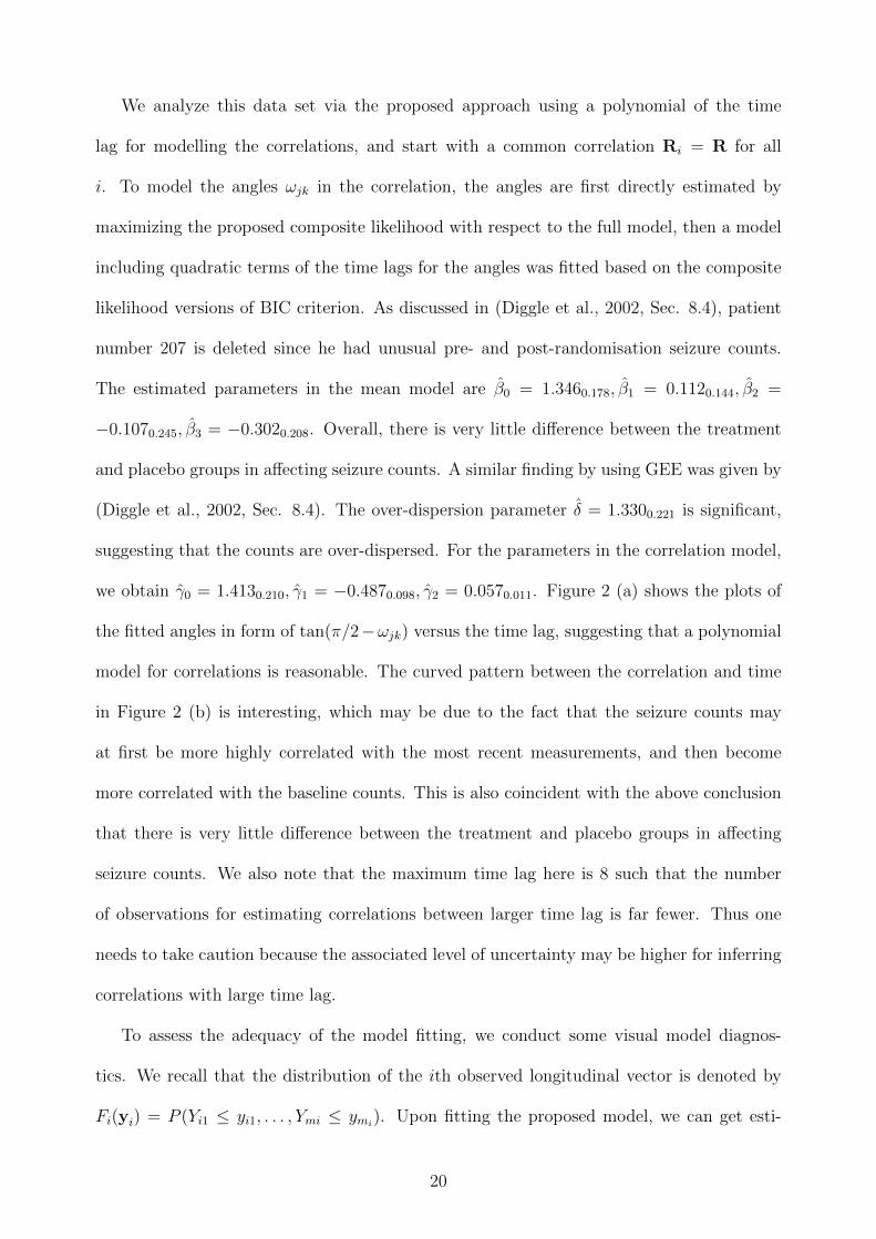
We analyze this data set via the proposed approach using a polynomial of the time

lag for modelling the correlations, and start with a common correlation Ri = R for all

i. To model the angles ωjk in the correlation, the angles are first directly estimated by

maximizing the proposed composite likelihood with respect to the full model, then a model

including quadratic terms of the time lags for the angles was fitted based on the composite

likelihood versions of BIC criterion. As discussed in (Diggle et al., 2002, Sec. 8.4), patient

number 207 is deleted since he had unusual pre- and post-randomisation seizure counts.

The estimated parameters in the mean model are β0 = 1.3460.178, β1 = 0.1120.144, β2 =

−0.1070.245, β3 = −0.3020.208. Overall, there is very little difference between the treatment

and placebo groups in affecting seizure counts. A similar finding by using GEE was given by

(Diggle et al., 2002, Sec. 8.4). The over-dispersion parameter δ = 1.3300.221 is significant,

suggesting that the counts are over-dispersed. For the parameters in the correlation model,

we obtain γ0 = 1.4130.210, γ1 = −0.4870.098, γ2 = 0.0570.011. Figure 2 (a) shows the plots of

the fitted angles in form of tan(π/2−ωjk) versus the time lag, suggesting that a polynomial

model for correlations is reasonable. The curved pattern between the correlation and time

in Figure 2 (b) is interesting, which may be due to the fact that the seizure counts may

at first be more highly correlated with the most recent measurements, and then become

more correlated with the baseline counts. This is also coincident with the above conclusion

that there is very little difference between the treatment and placebo groups in affecting

seizure counts. We also note that the maximum time lag here is 8 such that the number

of observations for estimating correlations between larger time lag is far fewer. Thus one

needs to take caution because the associated level of uncertainty may be higher for inferring

correlations with large time lag.

To assess the adequacy of the model fitting, we conduct some visual model diagnos-

tics. We recall that the distribution of the ith observed longitudinal vector is denoted by

Fi(yi) = P (Yi1 ≤ yi1, . . . , Ymi ≤ ymi). Upon fitting the proposed model, we can get esti-

20

mated probabilities denoted by F1,i(yi) (i = 1, . . . , n). On the other hand, we may calculate

empirical distribution by F2,i(yi) = n−1∑n

j=1 I(y1j ≤ y1i, . . . , ymj ≤ ymi). A plot of F1,i vs

F2,i can be an overall diagnostic of goodness of fit, and is given in (a) of Figure 3, showing an

overall reasonable fitting of the distribution. As a second diagnostic, we focus on the fitting

of the correlation structure. In particular, we compute the empirical correlations between

the z-scores, zij = Φ−1(F (yij)), and then we plot it against the fitted correlation with the

proposed method, which is given in (b) of Figure 3, indicating a reasonable fitting of the

correlation matrix Ri.

(a) (b)

Figure 3: plots of model diagnostics: (a) the empirical distribution function vs the fitteddistribution function; (b) the empirical correlations of the z-scores vs the fitted correlations.

4.3 Simulations

We conduct extensive simulations in this section to assess the performance of the mean-

correlation modeling methodology with R. We also compare the pairwise likelihood estimates

(PLEs) with the MLEs in terms of their biases and variances, and evaluate the accuracy

of the inferential procedure for estimating the standard errors of the estimators. As a

benchmark, we compare our method to the GEE method in Liang and Zeger (1986) for

estimating the parameters in the mean model and the dispersion, assuming unstructured

correlations. In each of the following studies, we generate 500 data sets and consider sample

21

sizes n = 50, 100 and 200. All simulations were conducted in R. We first report the difference

in time for obtaining the PLEs and MLEs for Study 1 when n = 50. We find that on the

average, it takes twice as much time to obtain the MLEs when mi = 4, twenty times as

such time when mi = 6. When mi = 8, the computational time becomes intractable for

the full likelihood approach. While for the pairwise likelihood approach, the computational

time is manageable even for larger mi. This highlights the substantial gain in terms of the

computational time by using pairwise likelihood.

Study 1. The data sets are generated from the model

yij ∼ Poisson(λij), log(λij) = β0 + xij1β1 + xij2β2,

ωijk = π/2− atan(γ0 + wijk1γ1 + wwjk2γ2), (i = 1, . . . , n; j = 1, . . . ,mi),

where the measurement times tij are generated from the uniform distribution. We consider

two cases: (I) mi ≡ 6 and (II) mi− 1 ∼ Binomial(6, 0.8) respectively. The latter case gives

different numbers of repeated measurements mi for different subjects. The covariate xij =

(xij1, xij2)T is generated from a standard bivariate normal distribution with zero correlation.

We take the covariates for the correlations as wijk = {1, tij−tik, (tij−tik)2}T. The parameters

are set as β = (β0, β1, β2) = (1.0,−0.5, 0.5) and γ = (γ0, γ1, γ2) = (0.5,−0.3, 0.5). There is

no dispersion parameter for this study.

Table 1 shows the accuracy of the estimated parameters in terms of their mean biases

(MB) and standard deviations. For PLEs, all the biases are small especially when n is large.

Additionally, to evaluate the inference procedure, we compare the sample standard deviation

(SD) of 500 parameter estimates to the sample average of 500 standard errors (SE) using

formula (11). The standard deviation (Std) of 500 standard errors is also reported. Table

1 shows that the SD and SE are quite close, especially for large n. This indicates that the

standard error formula works well and demonstrates the validity of Theorem 1. Although

estimators based on the pairwise likelihood function is slightly less efficient than the maxi-

mum likelihood estimates, they have smaller biases. In particular, the MLEs for estimating

22

the parameters in the correlation matrices are highly biased. As discussed earlier, this is

likely due to the computational difficulty of evaluating multidimensional integrals when a

full likelihood is used. Compared to the GEE estimates with unstructured correlations

for estimating the parameters in the mean model, the PLEs have very competitive perfor-

mance. Though our method is not designed with specific consideration for enhancing the

mean model estimation incorporating correlations from the longitudinal data, we see that

their performance is very close to those of the full likelihood and GEE methods. When the

sample size is smaller, the PLEs even outperform the GEE with unstructured correlations,

showing the advantage of using parsimonious correlation models.

We now assess the finite sample performance of the approximation results in Theorem

3 by testing H0 : β2 = 0 and H0 : γ0 = 0 respectively under simulation setup case I.

Figure 4 (a) and (b) display the power functions by the proposed pairwise likelihood ratio

testing procedure with a nominal level 0.05. It is clear that the size of the test is well

maintained at the nominal level and that the power of the test increases when the true

parameter value deviates from that in the null hypothesis. To examine the finite sample

distribution under the null provided by Theorem 3, Figure 4 (c) shows the Q-Q plot of

LRT = 2{pl(θ) − pl(θ)} based on 500 simulated data sets with sample size n = 50, for

testing H0 : θ1 = θ1,0 with θ1 = (β2, γ0)T and θ1,0 = (0, 0)T. The estimated null distribution

is found to be 4.81χ21 + 0.94χ2

1, where each eigenvalue is the average of 500 eigenvalues, one

from each simulation. Then we treat this distribution as the null distribution and obtain

its quantile via simulation as the theoretical quantiles. We further plot them against the

observed quantiles from the 500 pairwise likelihood ratio statistics. It is seen that there is

a close agreement between these two sets of quantiles, even though the sample size n = 50

is fairly small.

23

0.00 0.05 0.10 0.15 0.20

0.2

0.4

0.6

0.8

1.0

(a)

β2,0

Pow

er

0.0 0.1 0.2 0.3 0.4

0.2

0.4

0.6

0.8

1.0

(b)

γ0,0

Pow

er

●●●●●●●●●●●●●●

●●●●●●●●●●

●●●●●●●●●●●

●●●●●●●●●●●●●●●

●●●●●●●●

●●●●●●●●●●

●●●●●●

●●●●●●●●●●

●●●●●●●●

●●●●●●●

●●●●●●

●●●●●●●

●●●●

●●●●

●●●

●●●●●●●

●●●●●●●●

●●●●●

●●●

●●●

●●●●●

●●●

0 2 4 6 8

02

46

8

(c)

Theoretical Quantile

Obs

erve

d Q

uant

ile

Figure 4: (a) The power function for testing H0 : β2 = 0; (b) The power function for testingH0 : γ0 = 0; (c) Quantile-Quantile plot of the pairwise likelihood ratio statistics relative tothe mixture of χ2

1 distributions as in Theorem 3. The dashed horizontal lines are at the 0.05nominal level.

Study 2. The data sets are generated from the model

yij ∼ Bernoulli(pij), logit(pij) = β0 + xij1β1 + xij2β2,

ωijk = π/2− atan(γ0 + wijk1γ1 + wijk2γ2), (i = 1, . . . , n; j = 1, . . . ,mi),

where again mi ≡ 6 for case I and mi − 1 ∼ Binomial(6, 0.8) for case II. The measure-

ment times tij are generated from the uniform distribution. We set β = (β0, β1, β2) =

(1.0,−0.5, 0.5) and γ = (γ0, γ1, γ2) = (0.5,−0.3, 0.5). The covariate xij is generated again

from a standard normal distribution. we take wijk = {1, tij − tik, (tij − tik)2}T. Table 2

shows the results that are qualitatively similar to those in Study 1.

Study 3. This is a study designed for investigating the impact on the mean model

estimation from misspecified correlation model. For such a purpose, we generate data from

the following random effect Poisson regression model

yij ∼ Pois(λij), log(λij) = β0 + β1xij1 + β2xij2 + zijbi

where bi ∼ N(0, σ2b ) is a random effect accounting for the correlations. The β = (1, 0.5,−0.5)′

and σb = 0.8. The covariates xij1 and xij2 are generated from standard normal, zij ∼

Uniform(0, 1). The number of repeated measurements is 6. We applied the cubic polyno-

mial of time lag for our approach when modeling the correlations, and we have also compared

24

our approach with the GEE method with different specifications of the working correlation

structures. For this setting, the model is mis-specified for both our method and the GEE

method. The simulation results are summarized in Table 3. From the results, we can see

that our method performs very competitively, even when the correlation structure is not cor-

rectly specified. Specifically, when sample sizes are small, our method consistently performs

the best with the smallest MSE. When sample size is larger, the GEE with unstructured

covariance specification works very well. However, when sample size is smaller at n = 50,

the GEE with unstructured covariance specification has very high level of variation due to

unstable covariance estimations. Overall, our method performs very promisingly, indicating

the potential benefit for estimating the mean model incorporating the correlations between

the longitudinal data from using a parsimonious correlation model.

Summary. Through the simulations, we clearly see the merits of the proposed mean-

correlation regression approach in terms of gains from using parsimonious correlation mod-

eling, especially when the sample size is smaller. As for estimating the parameters in the

mean model, we see that the pairwise likelihood based method performs very competitively,

comparing with the full likelihood based approach and the GEE method that are capable

of incorporating correlation structures from the longitudinal data. This reflects that our

method is very effectively for estimating the mean model, also being capable of incorpo-

rating the correlation structures. In simulation results not reported here, we found very

substantial improvement of our method compared with the GEE with working indepen-

dence. We also find that inferences including estimations and hypothesis testing are highly

effective using the pairwise likelihood instead of using the computationally intractable full

likelihood. Hence, using our mean-correlation regression approach with pairwise likelihood

based inferences could provide a powerful and convenient device for analyzing generic dis-

crete longitudinal data in practice.

25

5 Conclusion

The problem of developing regression models for correlation structures is an open problem

when longitudinal responses are discrete. This paper proposes the first model of this kind to

address the challenging problem. Equipped with the new parametrization of a correlation

matrix in a copula model which enables unconstrained model building and a computationally

efficient estimation method based on pairwise likelihood, we have developed a new tool for

investigating correlated responses.

This paper focuses mainly on univariate discrete responses. It will be interesting to

generalize the univariate models to situations where multiple mixed outcomes are available

at each time point (Xu and Mackenzie, 2012). One way to simplify the multiple response

time-dependent covariance is to factorize the covariance matrices via a Kronecker product

decomposition that greatly reduces the dimensionality. This problem will be studied in a

future paper. Another interesting problem is to develop model diagnostic tools for assessing

model adequacy, especially for unbalanced data. For balanced data, as illustrated in the

paper, graphical tools to compare the empirical estimates and the model estimates, such as

those used for analyzing the toenail data and the epileptic seizure data, are useful. However,

counterparts of those are not currently available when data are unbalanced. Finally, this

proposed framework for modeling mean-correlation is extremely flexible and allows the de-

velopment of parametric, nonparametric, semi-parametric models for correlations. As such,

another future line of research is to develop data-driven models for covariations.

Acknowledgement

We thank the Editor, Associate Editor, and two referees for their constructive comments and

suggestions that have greatly improved the paper. Zhang acknowledges support from the

National Key Research and Development Plan (No. 2016YFC0800100 and the NSF of China

26

(No. 11671374,71631006). Tang acknowledges support from NSF Grants SES-1533956 and

IIS-1546087. Leng was supported by the Alan Turing Institute under the EPSRC grant

EP/N510129/1.

References

Bergsma, W., Croon, M., and Hagenaars, J. A. (2009), Marginal Models for Dependent,

Clustered, and Longitudinal Categorical Data, Springer.

Chib, S. and Greenberg, E. (1998). Analysis of multivariate probit models. Biometrika, 85,

347–361.

Creal, D., Koopman, S. J., and Lucas, A. (2011). A dynamic multivariate heavy-tailed

model for time-varying volatilities and correlations. Journal of Business and Economic

Statistics, 29, 552–563.

Daniels, M. J. and Pourahmadi, M. (2009). Modeling covariance matrices via partial auto-

correlations. Journal of Multivariate Analysis, 100, 2352–2363.

De Backer, M., De Keyser, P., De Vroey, C., and Lesaffre, E. (1996). A 12-week treatment

for dermatophyte toe onychomycosis: terbinafine 250mg/day vs. itraconazole 200mg/day

a double-blind comparative trial. British Journal of Dermatology, 134, 16–7.

Dickson, E. R., Grambsch, P. M., Fleming, T. R., Fisher, L. D. and Langworthy, A. (1989).

Prognosis in primary biliary cirrhosis: Model for decision making. Hepatology, 10, 1–7.

Diggle, P. J., Heagerty, P., Liang, K. Y., and Zeger, S. L. (2002). Analysis of Longitudinal

Data. Oxford University Press, 2nd edition.

Fan, J., Liu, H., Ning, Y., and Zou, H. (2017), High dimensional semiparametric latent

graphical model for mixed data. Journal of the Royal Statistical Society, Series B, 79, 405

- 421.

Fang, H., Fang, K., and Kotz, S. (2002). The meta-elliptical distributions with given

marginals. Journal of Multivariate Analysis, 82, 1-16.

Fitzmaurice, G. M., Laird, N. M., and Ware, J. H. (2004). Applied longitudinal analysis,

New York: Wiley.

Fleming, T. R. and Harrington, D. P. (1991). Counting Processes and Survival Analysis.

New York:Wiley.

Gao, X. and Song, P.X.K. (2010). Composite likelihood Bayesian information criteria for

model selection in high-dimensional data. Journal of the American Statistical Association,

105, 1531-1540.

Gaskins, J., Daniels, M.J., and Marcus, B. (2014). Sparsity inducing prior distributions

for correlation matrices of longitudinal data. Journal of Computational and Graphical

Statistics, 23, 966–984.

Hoffman, L. (2012). Considering alternative metrics of time: Dos anybody really know what

“time” is? In G. Hancock and J. R. Harring (Ed.) Advances in longitudinal methods in

27

the social and behavioral sciences. Charlotte, NC: Information Age Publishing.

Liu, H., Lafferty, J. D., and Wasserman, L. A.(2009). The nonparanormal: semiparametric

estimation of high dimensional undirected graphs. Journal of Machine Learning Research,

10, 2295-2328.

Leng, C., Zhang, W., and Pan, J. (2010). Semiparametric mean-covariance regression anal-

ysis for longitudinal data. Journal of the American Statistical Association, 105, 181–193.

Liang, K. Y. and Zeger, S. L. (1986). Longitudinal data analysis using generalized linear

models. Biometrika, 73, 13–22.

Lee, Y. and Nelder, J. A. (2006). Double hierarchical generalized linear models (with dis-

cussion). Journal of the Royal Statistical Society: Series C, 55, 139–185.

Lynn, P. (2009). Methodology of Longitudinal Surveys, Wiley.

McCullagh, P. and Nelder, J. A. (1989). Generalized Linear Models, New York: Chapman

and Hall/CRC.

Molenberghs, G. and Verbeke, G. (2005). Models for Discrete Longitudinal Data. Springer-

Verlag.

Muenz, L. R. and Rubinstein, L. V. (1985). Markov models for covariate dependence of

binary sequences. Biometrics, 41, 91–101.

Pan, J. and Mackenzie, G. (2003). Model selection for joint mean-covariance structures in

longitudinal studies. Biometrika, 90, 239–244.

Pourahmadi, M. (1999). Joint mean-covariance models with applications to longitudinal

data: unconstrained parameterisation. Biometrika, 86, 677–690.

Pourahmadi, M. (2000). Maximum likelihood estimation of generalised linear models for

multivariate normal covariance matrix. Biometrika, 87, 425–35.

Pourahmadi, M. (2007). Cholesky decompositions and estimation of a covariance matrix:

Orthogonality of variance-correlation parameters. Biometrika, 94, 1006–1013.

Pourahmadi, M. (2011). Covariance estimation: The GLM and regularization perspectives.

Statistical Science, 26, 369–387.

Song, P. X.-K., Li, M., and Yuan, Y. (2009). Joint regression analysis of correlated data

using Gaussian copulas. Biometrics, 65, 60–68.

Song, P. X. K. (2000). Multivariate Dispersion Models Generated From Gaussian Copula.

Scandinavian Journal of Statistics, 27, 305 - 320.

Thall, P. F. and Vail, S. C. (1990). Some covariance models for longitudinal count data with

over-dispersion. Biometrics, 46, 657–671.

Tong, Y. L. (1990). The Multivariate Normal Distribution, Springer.

Varin, C., Reid, N., and Firth, D. (2011). An overview of composite likelihood methods.

Statistica Sinica, 21, 5–42.

Wang, Y. and Daniels, M. J. (2013). Bayesian modeling of the dependence in longitudinal

data via partial autocorrelations and marginal variances. Journal of Multivariate Analysis,

28

116, 130–140.

White, H. (1982). Maximum likelihood estimation of misspecified models. Econometrica, 50,

1–25.

Xu, J. and Mackenzie, G. (2012). Modelling covariance structure in bivariate marginal mod-

els for longitudinal data. Biometrika, 99, 649–662.

Ye, H. and Pan, J. (2006). Modelling covariance structures in generalized estimating equa-

tions for longitudinal data. Biometrika, 93, 927–941.

Zeger, S. L., Liang, K. Y., and Self, S. G. (1985). The analysis of binary longitudinal data

with timeindependent covariates. Biometrika, 72, 31–38.

Zeger, S. L. and Liang, K. Y. (1986). Longitudinal data analysis for discrete and continuous

outcomes. Biometrics, 42, 121–130.

Zhang, W. and Leng, C. (2012). A moving average cholesky factor model in covariance

modeling for longitudinal data. Biometrika, 99, 141–150.

Zhang, W., Leng, C., and Tang, C. Y. (2015). A joint modeling approach for longitudinal

studies. Journal of the Royal Statistical Society Series B, 77, 219–238.

29

Table 1: Simulation results for Study 1. Mean bias (MB) and standard deviation (SD) ofeach parameter us reported. SE is the average standard error calculated using the formulain Theorem 2. PL: Partial Likelihood; FL: Full Likelihood; GEE: Generalized EstimatingEquation.

Pairwise Likelihood Full Likelihood GEEn 50 100 200 50 100 200 50 100 200

Case IMBβ0

-0.007 -0.003 0.001 -0.006 -0.005 0.001 -0.014 -0.007 -0.001SD (0.073) (0.046) (0.034) (0.071) (0.046) (0.033) (0.076) (0.051) (0.034)SE 0.069 0.049 0.034 - - - - - -Std (0.005) (0.002) (0.001) - - - - - -MBβ1 -0.002 -0.001 0.000 -0.002 -0.001 0.000 -0.005 -0.001 0.001SD (0.033) (0.022) (0.015) (0.031) (0.021) (0.014) (0.037) (0.021) (0.016)SE 0.032 0.023 0.016 - - - - - -Std (0.004) (0.002) (0.001) - - - - - -MBβ2

0.002 0.001 0.000 0.002 0.001 0.000 0.003 0.002 0.000SD (0.034) (0.022) (0.016) (0.032) (0.020) (0.015) (0.038) (0.021) (0.015)SE 0.032 0.023 0.016 - - - - - -Std (0.004) (0.002) (0.001) - - - - - -MBγ0 0.001 -0.001 -0.004 -0.039 -0.046 -0.047 - - -SD (0.119) (0.078) (0.056) (0.069) (0.050) (0.036) - - -SE 0.090 0.063 0.044 - - - - - -Std (0.013) (0.007) (0.003) - - - - - -MBγ1 -0.023 -0.011 0.031 0.304 0.328 0.350 - - -SD (0.688) (0.462) (0.330) (0.301) (0.241) (0.181) - - -SE 0.477 0.332 0.232 - - - - - -Std (0.088) (0.048) (0.023) - - - - - -MBγ2 0.058 0.035 -0.024 -0.359 -0.378 -0.407 - - -SD (0.814) (0.555) (0.391) (0.340) (0.279) (0.212) - - -SE 0.558 0.385 0.268 - - - - - -Std (0.116) (0.063) (0.032) - - - - - -

Case IIMBβ0

-0.002 -0.002 -0.003 -0.004 -0.001 -0.002 -0.006 -0.004 -0.005SD (0.071) (0.053) (0.0360) (0.067) (0.050) (0.034) (0.087) (0.052) (0.034)SE 0.074 0.052 0.036 - - - - - -Std (0.006) (0.003) (0.001) - - - - - -MBβ1

0.001 -0.001 -0.001 0.001 -0.000 -0.000 -0.003 -0.002 -0.002SD (0.034) (0.026) (0.018) (0.033) (0.025) (0.017) (0.065) (0.025) (0.019)SE 0.036 0.026 0.018 - - - - - -Std (0.005) (0.002) (0.001) - - - - - -MBβ2

-0.001 0.001 0.001 -0.001 0.001 0.000 -0.000 -0.001 0.001SD (0.035) (0.025) (0.018) (0.033) (0.024) (0.017) (0.054) (0.026) (0.019)SE 0.036 0.023 0.018 - - - - - -Std (0.005) (0.002) (0.001) - - - - - -MBγ0 0.015 -0.001 -0.003 -0.037 -0.049 -0.048 - - -SD (0.132) (0.099) (0.065) (0.077) (0.053) (0.041) - - -SE 0.110 0.076 0.054 - - - - - -Std (0.017) (0.009) (0.004) - - - - - -MBγ1 -0.084 -0.011 0.009 0.326 0.372 0.362 - - -SD (0.795) (0.580) (0.388) (0.298) (0.195) (0.173) - - -SE 0.588 0.406 0.288 - - - - - -Std (0.117) (0.060) (0.030) - - - - - -MBγ2 0.132 0.034 -0.005 -0.386 -0.441 -0.442 - - -SD (0.963) (0.689) (0.464) (0.347) (0.209) (0.189) - - -SE 0.700 0.479 0.338 - - - - - -Std (0.162) (0.080) (0.043) - - - - - -

30

Table 2: Simulation results for Study 2. Mean bias (MB) and standard deviation (SD) ofeach parameter us reported. SE is the average standard error calculated using the formulain Theorem 2. PL: Partial Likelihood; FL: Full Likelihood; GEE: Generalized EstimatingEquation.

Pairwise Likelihood Full Likelihood GEEn 50 100 200 50 100 200 50 100 200

Case IMBβ0

0.009 0.016 0.005 0.029 0.033 0.023 0.0311 0.033 0.014SD (0.234) (0.153) (0.111) (0.227) (0.147) (0.105) (0.280) (0.160) (0.112)SE 0.220 0.156 0.110 - - - - - -Std (0.016) (0.008) (0.004) - - - - - -MBβ1 -0.014 -0.006 -0.002 -0.017 -0.011 -0.005 0.021 -0.001 0.003SD (0.152) (0.111) (0.076) (0.144) (0.107) (0.072) (0.168) (0.112) (0.072)SE 0.147 0.104 0.073 - - - - - -Std (0.018) (0.009) (0.004) - - - - - -MBβ2

0.021 0.004 0.006 0.025 0.008 0.010 -0.013 -0.004 0.001SD (0.153) (0.114) (0.077) (0.146) (0.107) (0.072) (0.167) (0.112) (0.073)SE 0.148 0.104 0.073 - - - - - -Std (0.017) (0.009) (0.004) - - - - - -MBγ0 -0.005 -0.004 0.004 -0.056 -0.048 -0.048 - - -SD (0.266) (0.179) (0.119) (0.141) (0.095) (0.065) - - -SEStd 0.203 0.143 0.100 - - - - - -Std (0.039) (0.019) (0.008) - - - - - -MBγ1 0.003 0.046 -0.013 0.343 0.329 0.324 - - -SD (1.562) (1.031) (0.728) (0.495) (0.270) (0.199) - - -SE 1.042 0.721 0.505 - - - - - -Std (0.205) (0.106) (0.051) - - - - - -MBγ2 0.139 -0.006 0.037 -0.338 -0.368 -0.365 - - -SD (1.919) (1.251) (0.871) (0.504) (0.272) (0.196) - - -SE 1.232 0.837 0.583 - - - - - -Std (0.276) (0.137) (0.068) - - - - - -

Case IIMBβ0

0.013 0.014 -0.002 0.024 0.031 0.017 0.044 0.030 0.007SD (0.240) (0.166) (0.117) (0.224) (0.157) (0.106) (0.244) (0.169) (0.115)SE 0.233 0.166 0.118 - - - - - -Std (0.020) (0.010) (0.005) - - - - - -MBβ1

-0.014 -0.006 -0.002 -0.017 -0.006 -0.005 -0.005 0.002 -0.001SD (0.168) (0.116) (0.084) (0.166) (0.114) (0.0768) (0.177) (0.116) (0.080)SE 0.165 0.117 0.082 - - - - - -Std (0.024) (0.011) (0.005) - - - - - -MBβ2

0.005 0.010 0.004 0.011 0.013 0.007 -0.005 0.004 0.002SD (0.174) (0.120) (0.084) (0.166) (0.115) (0.080) (0.175) (0.119) (0.081)SE 0.166 0.117 0.082 - - - - - -Std (0.022) (0.011) (0.005) - - - - - -MBγ0 0.009 -0.009 -0.008 -0.043 -0.058 -0.054 - - -SD (0.329) (0.207) (0.140) (0.172) (0.109) (0.073) - - -SE 0.240 0.166 0.117 - - - - - -Std (0.052) (0.023) (0.011) - - - - - -MBγ1 -0.032 0.004 0.054 0.315 0.035 0.354 - - -SD (2.001) (1.207) (0.833) (0.553) (0.109) (0.194) - - -SE 1.249 0.869 0.604 - - - - - -Std (0.260) (0.126) (0.064) - - - - - -MBγ2 0.164 0.095 -0.022 -0.334 -0.363 -0.392 - - -SD (2.531) (1.558) (1.011) (0.587) (0.3522) (0.167) - - -SE 1.497 1.024 0.709 - - - - - -Std (0.346) (0.173) (0.085) - - - - - -

31

Table 3: Simulation results. Mean bias (MB) and Mean square error (MSE) of each param-eter is reported under different sample sizes and models. PL: pairwise likelihood approach;GEE: generalized estimating equations; Ind: Independent working correlation; AR: AR(1)working correlation; Unstr: Unstructured working correlation. All results are multiplied by100.

nMBβ0MSE MBβ1

MSE MBβ2MSE

PL50 10.09 2.04 -0.26 0.45 -0.12 1.57

100 11.28 1.66 -0.21 0.21 0.15 0.93150 9.72 1.27 -0.54 0.12 0.12 0.48

GEE

Ind50 10.27 2.17 0.26 0.54 -0.3 1.88

100 11.27 1.68 0.08 0.21 -0.75 1.06150 10.68 1.51 -0.42 0.15 -0.41 0.59

AR50 10.50 2.16 -0.13 0.45 -0.31 1.67

100 11.29 1.65 -0.08 0.17 -1.06 0.85150 10.67 1.48 -0.49 0.13 -0.08 0.42

Unstr50 8.43 6.12 -1.30 3.65 0.37 6.24

100 10.78 1.54 -0.02 0.17 -1.02 0.91150 10.23 1.37 -0.42 0.13 -0.17 0.45

32

Supplementary Material to “Discrete Longitudinal Data Modeling with a

Mean-Correlation Regression Approach”

Tang, C.Y., Zhang, W., and Leng, C.

This Supplementary Material contains technical proofs, additional data analysis and

simulations studies.

Computation of the score function. Note that the objective function is

pl(θ) =n∑

i=1

∑1≤j<k≤mi

lijk(θ),

where

lijk(θ) = logLijk(θ) = log

∫ zij

z−ij

∫ zik

z−ik

φ2(u; ρijk)du

= log(

Φ2(zij, zik; ρijk)− Φ2(z−ij , zik; ρijk)− Φ2(zij, z

−ik; ρijk) + Φ2(z

−ij , z

−ik; ρijk)

)and Φ2(x, y; ρ) is the cdf of bivariate normalN(0, 0, 1, 1, ρ), zij = Φ−11 {F (yij)} = zij(β, ψ), z−ij =

Φ−11 {F (yij − 1) = z−ij(β, ψ)}, and denote η = (βT, ψ)T. We have

∂lijk∂η

=1

Lijk

∂Lijk

∂η=

1

Lijk

( ∂

∂ηΦ2(zij, zik; ρijk)− ∂

∂ηΦ2(z

−ij , zik; ρijk)

− ∂

∂ηΦ2(zij, z

−ik; ρijk) +

∂

∂ηΦ2(z

−ij , z

−ik; ρijk)

). (A.1)

By the fact that

∂Φ2(z1, z2; ρ)

∂η=∂Φ2(z1, z2; ρ)

∂z1

∂z1∂η

+∂Φ2(z1, z2; ρ)

∂z2

∂z2∂η

= φ(z1)Φ1

( z2 − ρz1√1− ρ2

)∂z1∂η

+ φ(z2)Φ1

( z1 − ρz2√1− ρ2

)∂z2∂η

= Φ1

( z2 − ρz1√1− ρ2

)∂F (y1)

∂η+ Φ1

( z1 − ρz2√1− ρ2

)∂F (y2)

∂η, (A.2)

where zi = Φ−11 {F (yi)}, i = 1, 2, we can write out (A.1) easily.

Noting that for j < k, ρijk =∑j

s=1 TijsTiks and

∂Tits∂γ

=

Tits[−tan(ωits)

∂ωits

∂γ +∑s−1

l=11

tan(ωitl)∂ωitl

∂γ ] t > s > 1

Tits∑s−1

l=11

tan(ωitl)∂ωitl

∂γ , t = s > 1

−sin(ωit1)∂ωit1

∂γ , s = 1

,

1

we can obtain the derivative of lijk with respect to γ as

∂lijk∂γ

=1

Lijk

∂Lijk

∂γ=

1

Lijk

(φ2(zij, zik; ρijk)− φ2(z

−ij , zik; ρijk)

− φ2(zij, z−ik; ρijk) + φ2(z

−ij , z

−ik; ρijk)

)∂ρijk∂γ

. (A.3)

Combining (A.1) and (A.3) leads to the score function Sn(θ) .

The expected Hessian matrix. For the second derivatives of log-likelihood function,

the formula is more complicated. However, it is easy to see that

EHn(θ) = − 1

n

n∑i=1

∑1≤j<k≤mi

Elijk(θ)

=1

n

n∑i=1

∑1≤j<k≤mi

Elijk(θ)lTijk(θ), (A.4)

thus Hn in (10) can be approximated by 1n

∑ni=1

∑1≤j<k≤mi

lijk(θ)lTijk(θ).

Proof of Theorem 1. The proof follows as a special case of the following proof for

Theorem 2, and hence is omitted.

Proof of Theorem 2. Here we give a sketch of the proof. It is easy to see that

EθSn(θ) = 0. Thus by Taylor expansion, we have

0 = Sn(θ) = Sn(θ0) + Sn(θ)(θ − θ0),

where Sn = ∂ST

n/∂θ and θ is in a neighborhood of θ0. Specially, we have θ → θ0 when

n→∞. Therefore, it is seen that

√n(θ − θ0) = [− 1

nSn(θ)]−1

1√nSn(θ0).

From Central Limit Theorem, Assumption A1-A3, Eθ0Sn(θ0) = 0 and the boundness of

V arθ0(Sni(θ0)), i = 1, . . . , n, we have

1√nSn(θ0)→ N(0,J(θ0)).

By Assumption A3 and Slutsky’s theorem, θ is consistent and asymptotically normal with

asymptotic covariance matrix G(θ0).

Proof of Theorem 3. Using a Taylor expansion of the log-pairwise likelihood function

pl around θ, we obtain

pl(θ) = pl(θ) + (θ − θ)TSn(θ) +1

2(θ − θ)T(−nH(θ))(θ − θ) + op(1).

2

Notice that 0 = Sn(θ) = Sn(θ) + (−nH(θ))(θ − θ) + op(n1/2). We then have

pl(θ) = pl(θ) +n

2(θ − θ)TH(θ)(θ − θ) + op(1).

It can be rewritten via a partitioned matrix notation

pl(θ1, θ2) = pl(θ1,θ2)

+n

2((θ1 − θ1)T, (θ2 − θ2)T)

H11 H12

H21 H22

θ1 − θ1

θ2 − θ2

+ op(1). (A.5)

Assuming that the null hypothesis is true, a Taylor expansion of the score Sn,2 around

(θ1,0,θ2) gives

0 = Sn,2(θ1,0, θ2) = Sn,2(θ1,0,θ2) + (−nH22)(θ2 − θ2) + op(n1/2).

Equating this with the corresponding part of Sn(θ1,0,θ2), we find

θ2 − θ2 = H−122 H21(θ1 − θ1,0) + (θ2 − θ2) + op(n1/2).

Therefore under the null hypothesis, it is true that

2{pl(θ1,0, θ2)− pl(θ1,0, θ2)} = n(θ2 − θ2)TH22(θ1,0,θ2)(θ2 − θ2) + op(1)

= n[(θ1 − θ1,0)H12H−122 H21(θ1 − θ1,0) + 2(θ1 − θ1,0)TH12(θ2 − θ2)

+ (θ2 − θ2)TH22(θ2 − θ2)] + op(1). (A.6)

Combing (A.5) and (A.6) we have

2{pl(θ)− pl(θ1,0, θ2)} = 2{pl(θ)− pl(θ1,0,θ2)} − 2{pl(θ1,0, θ2)− pl(θ1,0, θ2)}

= n(θ1 − θ1,0)T(H11 −H12H−122 H21)(θ1 − θ1,0) + op(1)

= n(θ1 − θ1,0)T(H11)−1(θ1 − θ1,0) + op(1).

Because under the null hypothesis√n(θ1−θ1,0)→ N(0,G11), it follows from the properties

of a multivariate normal distribution that

n(θ1 − θ1,0)T(H11)−1(θ1 − θ1,0)d→

r∑j=1

λjVj,

where V1, . . . , Vr denote independent χ21 random variables and λ1 ≥ · · · ≥ λr are the eigen-

values of (H11)−1G11. The proof is completed.

3

Toenail data

We apply our mean-correlation regression method to analyze a data set from the toenail

dermatophyte onychomycosis study (De Backer et al., 1996). This data set consists of

294 participants in two treatment groups with a total of 1907 observations. Subjects were

initially examined every month during a 12-week (3 months) treatment period, and then

followed up further every 3 months for up to a total of 48 weeks (12 months). Due to

various unknown reasons, in total there are 23.8% subjects dropping out, and consequently

measurement numbers per subject range from 1 to 7. Therefore, this data set is unbalanced.

The response variable of interest for our analysis is the severity of the infection of the toenail,

coded as 0 (not severe) or 1 (severe). By analyzing this response variable, one aims to reveal

the trend of the infection severity over time, and compare patterns, if any, between the two

treatment groups. Following Molenberghs and Verbeke (2005), in the marginal model, we

use the following logistic model for the conditional mean function for the jth measurements

of the ith subject:

Yij ∼ Bernoulli(πij), logit(πij) = β0 + β1Ti + β2tij + β3Titij,

where Ti is the treatment indicator for subject i (1 for the experimental arm, 0 for the

standard arm), tij is the time point at which the jth measurement is taken for the ith

subject.

As for the correlation modeling, considering that the data set is unbalanced with homo-

geneously spaced time points for all subjects, we first investigate a reasonable model using a

common 7× 7 correlation matrix R by letting Ri = R for all subjects. Thus the equivalent

unknown parameters for R by the parametrization (4) are ωjk (1 ≤ j < k ≤ 7). Then the

pairwise likelihood approach is applied to obtain estimators ωjk, leading to an estimated

correlation matrix. The plot of the function tan(π/2 − ωjk) versus the time lag is given in

Figure 5 (a) with solid dots, suggesting some monotone decreasing associations. Clearly,

this method for incorporating the correlations involves 7× 6/2 = 21 parameters.

Now let us demonstrate the application of the parsimonious correlation regression. Sug-

gested by Figure 5 (a) and the composite likelihood versions of Bayesian information crite-

rion (BIC) described by Gao and Song (2010), we link these angles with covariates via the

parsimonious model specified in (5) using a quadratic polynomial function of the time lag

4

between measurements with unknown parameters γ0, γ1, γ2. The estimated parameters of

the mean-correlation joint model with estimated standard deviation shown in the subscript

are β0 = −0.55650.1711, β1 = 0.02360.2407, β2 = −0.18300.0232, β3 = −0.07740.0344, suggest-

ing that the time is a significant covariate in the mean model, while the evidence for the

treatment effect and its interaction with time is not statistically significant. For compar-

isons, we also obtain a GEE estimates of the parameters in the same mean model with

unstructured working correlations: β0 = −0.68980.1679, β1 = 0.08280.2430, β2 = −0.14830.0283

and β3 = −0.10430.0514. We found that the two sets of estimates are largely compara-

ble with each other. The estimated parameters in the correlation regression model are

γ0 = 3.02360.2750, γ1 = −0.46900.0658, γ2 = 0.02040.0043, all highly significant. Denoted by

ωjk the estimated angles from the parsimonious model, Figure 5 (a) also shows the plot of

the fitted angles tan(π/2− ωjk) versus time lag, which indicates a competent fitting of the

angles with far fewer parameters where only 3 parameters are involved compared with 21

parameters in a common correlation matrix R. Figure 5 (b) indicates, not surprisingly, that

the correlation decreases as the time lag increases, suggesting a high correlation between

the severity of the infection at current visit with the those at the nearest visit times.

●

●

●

●

●

●

●

●

●

●

●

●

●

●

●

●

●

●

●

●

●

2 4 6 8 10 12

01

23

45

(a)

Time Lag

tan(

π2

−ω

)

●

●

●

●

●

●

●

●

●

●

●

●

●

●

●

●

●

●

●

●

●

●

●●

●

●●

●

●

●

●

●

●

●

●

●

●

●

●

● ●

●

2 4 6 8 10 12

0.3

0.4

0.5

0.6

0.7

0.8

0.9

1.0

(b)

Time Lag

Cor

rela

tion

Figure 5: The toenail data: (a) plot of fitted angles tan(π/2 − ωjk) versus time lag, (b)plot of fitted correlations versus time lag. In panel (a), solid dots are fitted angles with acommon correlation matrix for all subjects with parametrization (4), the solid black lineis from fitting a LOWESS curve to the solid dots, the solid red line is from the proposedmodel, and the dashed curves represent asymptotic 95% confidence intervals.

5

Additional simulations

Study 4. We generate n observations y1, . . . ,yn, each with dimension mi set as the

two cases in Study 1. In this study we consider a Gaussian copula model in which the

marginal distributions Fij(j = 1, ...,m) are negative binomial as yij ∼ NegBin(δ, µij) with

mean µij and variance µij + µ2ij/δ, where δ > 0 is the over-dispersion parameter. The mean

is parameterised as µij = exp(xTijβ) to allow dependence on covariates, and the variance

exceeds its mean (i.e. overdispersion). The covariate xij1 and xij2 are generated from a

bivariate normal distribution with correlation 0.5. The angles in the correlation matrix is set

as ωijk = π/2−atan(γ0+wijk1γ1) with wijk = {1, tij−tik, (tij−tik)2}T. The true parameters

are taken as β = (β0, β1, β2) = (1,−0.5, 0.5), δ = 4 and γ = (γ0, γ1, γ2) = (0.5,−0.3, 0.5).

Table 4 shows that all the biases for the proposed method are small and that the SD

and SE are quite close, especially for large n. Interestingly, the MLEs perform slightly

better in this study for Case I, but we observed that it took much more time to obtain

them. For Case II, the large bias of the MLEs suggest again that the MLE may encounter

severe numerical problems when the multi-dimensional integrations are computed. In terms

of the estimation efficiency of the parameters in the mean model, the proposed PLEs again

performs very competitively compared with the GEE method with unstructured correlations

in this case.

6

Table 4: Simulation results for Study 4. Mean bias (MB) and standard deviation (SD) ofeach parameter us reported. SE is the average standard error calculated using the formulain Theorem 2. PL: Partial Likelihood; FL: Full Likelihood; GEE: Generalized EstimatingEquation.

Pairwise Likelihood Full Likelihood GEEn 50 100 200 50 100 200 50 100 200

Case IMBβ0

-0.002 -0.002 -0.001 -0.004 -0.004 -0.004 -0.008 -0.002 -0.001SD (0.047) (0.058) (0.046) (0.051) (0.063) (0.050) (0.093) (0.058) (0.044)SE 0.056 0.041 0.029 - - - - - -Std (0.006) (0.005) (0.003) - - - - - -MBβ1 0.008 -0.004 -0.003 0.004 -0.006 -0.004 -0.001 -0.001 -0.001SD (0.018) (0.031) (0.022) (0.024) (0.032) (0.024) (0.044) (0.027) (0.021)SE 0.032 0.023 0.016 - - - - - -Std (0.005) (0.003) (0.002) - - - - - -MBβ2

0.003 -0.002 -0.002 0.001 -0.004 -0.004 -0.002 0.001 -0.000SD (0.010) (0.035) (0.025) (0.019) (0.036) (0.025) (0.044) (0.030) (0.020)SE 0.032 0.023 0.016 - - - - - -Std (0.005) (0.003) (0.002) - - - - - -MBδ 0.561 0.313 0.111 0.282 0.395 0.224 1.407 0.791 0.500SD (0.746) (1.048) (0.640) (0.453) (1.138) (0.750) (2.559) (1.848) (1.416)SE 1.128 0.724 0.469 - - - - - -Std (0.382) (0.273) (0.103) - - - - - -MBγ0 -0.006 -0.004 -0.001 0.003 -0.091 -0.093 - - -SD (0.113) (0.079) (0.058) (0.025) (0.187) (0.193) - - -SE 0.100 0.073 0.051 - - - - - -Std (0.013) (0.007) (0.003) - - - - - -MBγ1 -0.019 -0.009 0.011 0.002 0.447 0.4318 - - -SD (0.654) (0.433) (0.332) (0.081) (0.459) (0.426) - - -SE 0.471 0.332 0.231 - - - - - -Std (0.083) (0.049) (0.022) - - - - - -MBγ2 0.052 0.022 -0.006 0.004 -0.413 -0.387 - - -SD (0.764) (0.522) (0.398) (0.112) (0.401) (0.329) - - -SE 0.549 0.384 0.266 - - - - - -Std (0.107) (0.066) (0.031) - - - - - -

Case IIMBβ0

-0.009 -0.001 -0.005 -0.010 0.001 -0.004 -0.012 0.000 -0.004SD (0.090) (0.068) (0.047) (0.088) (0.065) (0.045) (0.088) (0.065) (0.045)SE 0.031 0.020 0.014 - - - - - -Std (0.060) (0.027) (0.013) - - - - - -MBβ1

0.000 -0.001 -0.001 0.000 0.000 -0.001 -0.001 0.000 -0.001SD (0.046) (0.032) (0.023) (0.044) (0.031) (0.022) (0.046) (0.031) (0.023)SE 0.037 0.026 0.018 - - - - - -Std (0.007) (0.004) (0.002) - - - - - -MBβ2 -0.001 -0.001 0.000 -0.000 -0.000 0.000 -0.001 -0.000 0.000SD (0.049) (0.032) (0.024) (0.046) (0.030) (0.022) (0.047) (0.031) (0.024)SE 0.037 0.026 0.019 - - - - - -Std (0.007) (0.004) (0.002) - - - - - -MBδ 0.777 0.310 0.120 0.864 0.405 0.228 1.340 0.0.907 0.600SD (1.953) (1.051) (0.659) (2.073) (1.176) (0.831) (2.624) (1.984) (1.461)SE 1.358 0.770 0.502 - - - - - -Std (0.944) (0.306) (0.123) - - - - - -MBγ0 -0.001 -0.011 -0.005 -0.063 -0.070 -0.057 - - -SD (0.145) (0.067) (0.070) (0.114) (0.056) (0.069) - - -SE 0.125 0.086 0.061 - - - - - -Std (0.019) (0.008) (0.005) - - - - - -MBγ1 -0.042 -0.044 0.021 0.407 0.458 0.379 - - -SD (0.826) (0.096) (0.382) (0.550) (0.086) (0.364) - - -SE 0.591 0.403 0.285 - - - - - -Std (0.118) (0.061) (0.032) - - - - - -MBγ2 0.070 -0.037 -0.018 -0.477 -0.520 -0.442 - - -SD (0.994) (0.657) (0.451) (0.643) (0.480) (0.418) - - -SE 0.704 0.475 0.335 - - - - - -Std (0.165) (0.081) (0.043) - - - - - -

7