Manual On Setting Up, Using, And Understanding Random Forests V3.1

The V3.1 version of random forests contains some modificationsand major additions to Version 3.0. It fixes a bad bug in V3.0. Itallows the user to save the trees in the forest and run other data setsthrough this forest. It also allows the user to save parameters andcomments about the run.

I apologize in advance for all bugs and would like to hear aboutthem. To find out how this program works, read my paper "RandomForests" Its available on the same web page as this manual. It wasrecently published in the Machine Learning. Journal

The program is written in extended Fortran 77 making use of anumber of VAX extensions. It runs on SUN workstations f77 and onAbsoft Fortran 77 (available for Windows) and on the free g77compiler. but may have hang ups on other f77 compilers. If youfind such problems and fixes for them, please let me know.

Random forests computesclassification and class probabilitiesintrinsic test set error computationprincipal coordinates to use as variables.variable importance (in a number of ways)proximity measures between casesa measure of outlyingnessscaling displays for the data

The last three can be done for the unsupervised case i.e. no classlabels. I have used proximities to cluster data and they seem to doa reasonable job. The new addition uses the proximities to dometric scaling of the data. The resulting pictures of the data areinteresting and useful.

The first part of this manual contains instructions on how to set upa run of random forests V3.1. The second part contains the noteson the features of random forests V3.1 and how they work.

I. Setting Parameters

The first seven lines following the parameter statement need to befilled in by the user.

Line 1 Describing The Data

m d i m =number of variablesnsample0=number of cases (examples or instances) in the datanclass=number of classesmaxcat=the largest number of values assumed by a categorical

variable in the datantest=the number of cases in the test set. NOTE: Put ntest=1 if

there is no test set. Putting ntest=0 may cause compiler complaints .

labelts=0 if the test set has no class labels, 1 if the test set has classlabels.

iaddcl=0 if the data has class labels. If not, iaddcl=1 or 2adds a synthetic class as described below

If their are no categorical variables in the data set maxcat=1. Ifthere are categorical variables, the number of categories assumedby each categorical variable has to be specified in an integer vectorcalled cat, i.e. setting cat(5)=7 implies that the 5th variable is acategorical with 7 values. If maxcat=1, the values of cat areautomatically set equal to one. If not, the user must fill in thevalues of cat in the early lines of code.

For a J-class problem, random forests expects the classes to benumbered 1,2, ...,J. For an L valued categorical, it expects thevalues to be numbered 1,2, ... ,L. At present, L must be less than orequal to 32.

A test set can have two purposes--first: to check the accuracy of RFon a test set. The error rate given by the internal estimate will bevery close to the test set error unless the test set is drawn from adifferent distribution. Second: to get predicted classes for a set ofdata with unknown class labels. In both cases the test set musthave the same format as the training set. If there is no class labelfor the test set, assign each case in the test set label classs #1, i.e.put cl(n)=1, and set labelts=0. Else set labelts=1.

If the data has no class labels, addition of a synthetic class enables it

it to be treated as a two-class problem with nclass=2. Settingiaddclass=1 forms the synthetic class by independent samplingfrom each of the univariate distributions of the variables in theoriginal data. Setting iaddclass=2 forms the synthetic class byindependent sampling from uniforms such that each uniform hasrange equal to the range of the corresponding variable.

Line 2 Setting up the run

jbt=number of trees to growmtry=number of variables randomly selected at each nodelook=how often you want to check the prediction erroripi=set priorsndsize=minimum node size

jb t :this is the number of trees to be grown in the run. Don't bestingy--random forests produces trees very rapidly, and it does nothurt to put in a large number of trees. If you want auxiliaryinformation like variable importance or proximities growa lot of trees--say a 1000 or more. Sometimes, I run out to 5000trees if there are many variables and I want the variablesimportances to be stable.

m t r y :this is the only parameter that requires some judgment to set, butforests isn't too sensitive to its value as long as it's in the right ballpark. I have found that setting mtry equal to the square root ofmdim gives generally near optimum results. My advice is to beginwith this value and try a value twice as high and half as lowmonitoring the results by setting look=1 and checking the internaltest set error for a small number of trees. With many noisevariables present, mtry has to be set higher.

l o o k :random forests carries along an internal estimate of the test seterror as the trees are being grown. This estimate is outputted tothe screen every look trees. Setting look=10, for example, gives theinternal error output every tenth tree added. If there is a labeledtest set, it also gives the test set error. Setting look=jbt+1eliminates the output. Do not be dismayed to see the error ratesfluttering around slightly as more trees are added. Their behavior

is analagous to the sequence of averages of the number of heads intossing a coin.

ipi: pi is an real-valued vector of length nclass which sets priorprobabilities for classes. ipi=0 sets these priors equal to the classproportions. If the class proportions are very unbalanced, you maywant to put larger priors on the smaller classes. If differentweightings are desired, set ipi=1 and specify the values of the {pi(j)}early in the code. These values are later normalized, so settingpi(1)=1, pi(2)=2 weights a class 2 instance twice as much as a class1 instance. The error rates reported are an unweighted count ofmisclassified instances.

ndsize: setting this to the value k means that no node with fewerthan k cases will be split. The default that always gives goodperformances is ndsize=1. In large data sets, memory requirementswill be less and speed enchanced if ndsize is set larger. Usually, thisresults in only a small loss of accuracy for large data sets.

Line 3 Options on Variable Importance

im p =1 turns on the variable importances methods described below.

impstd=1 gives the standard imp outputimpmargin=1 gives, for each case, a measure of the effect ofnoising up each variableimpgraph=1 gives for each variable, a plot of the effect of the variable on the class probabilities.

impstd=1 computes and prints the following columns to a filei) variable numbervariables importances computed as:ii) The % rise in error over the baseline error.iii) 100* the change in the margins averaged over all casesiv) The proportion of cases for which the margin is decreased minus the proportion of increases.v) The gini increase by variable for the run

impgraph=1 computes and prints out the columns for eachvariable m--

i) variable number i.e. mii) sorted values of x(m) from lowest to highestiii-iii+nclass) effect of x(m) on the probabilities of class j.

Line 4 Options based on proximities

iprox=1 turns on the computation of the intrinsic proximitymeasures between any two cases . This has to be turned on forthe following options to work.

noutlier=1 computes an outlyingness measure for all cases in thedata. If iaddcl=1 then the outlyingness measure is computed onlyfor the original data. The output has the columns :

i) classii) case numberiii) measure of outlyingness

iscale=1 computes scaling coordinates based on the proximitymatrix. If iaddcl is turned on, then the scaling is outputted only forthe original data. The output has the columns:

i) case numberi) true classiii) predicted class.iv) 0 if ii)=iii), 1 otherwisev-v+msdim ) scaling coordinates

m d i m s c is the number of scaling coordinates to be extracted.Usually 4-5 is sufficient

Line 5 Transform to Principal Coordinates

ipc=1 takes the x-values and computes principal coordinates fromthe covariance matrix of the x's. These will be the new variables forRF to operate on. This will not work right if some of the variablesare categorical.

mdimpc: This is the number of principal components to extract.It has to be <=mdim.

norm=1 normaizes all of the variables to mean zero and sd onebefore computing the principal components.

Line 6 Saving the forest

isavef=1 saves all the trees in the forest to a file named eg. A.

isavep=1 creates a file B that contains the parameters usedin the run and allows up to 500 characters of text descriptionabout the run.

irunf=1 reads file A and runs new data down the forest.

i showp=1 reads file B and prints it to the sccreen

The calling code and files names required (except for the name ofA) are at the end of the main program. The name for A is enteredat the beginning of the program.

Line 7 Output Controls

Note: user must supply file names for all output listed belowor send it to the screen.

nsumout=1 writes out summary data to the screen. This includeserrors rates and the confusion matrix

infout=1 prints the following columns to a filei) case numberii) 1 if predicted class differs from true class, 0 elseiii) true class labeliv) predicted class labelv) margin=true class prob. minus the max of the other class prob.vi)-vi+nclass) class probabilities

ntestout=1 prints the follwing coumns to a filei) case number in test setii) true class (true class=1 if data is unlabeled)iii) predicted classiv-iv+nclass) class probabilities

iproxout=1 prints to filei) case #1 numberii) case #2 numberiii) proximity between case #1 and case #2

USER WORK:

The user has to construct the read-in the data code of which I haveleft an example. This needs to be done after the dimensioning ofarrays. If maxcat >1 then the categorical values need to be filled in.If ipi=1, the user needs to specify the relative weights of the classes.

File names need to be specified for all output. This is importantsince a chilling message after a long run is "file not specified" orsomething similar.

REMARKS:

The proximities can be used in the clustering program of yourchoice. Their advantage is that they are intrinsic rather than an adhoc measure. I have used them in some standard and home-brewclustering programs and gotten reasonable results. The proximitiesbetween class 1 cases in the unsupervised situation can be used tocluster. Extracting the scaling coordinates from the proximities andplotting scaling coordinate i versus scaling coordinate jgives illuminating pictures of the data. Usually, i=1 and j=2 give themost information (see the notes below).

There are four measures of variable importance: They complementeach other. Except for the 4th they are based on the test sets left outon each tree construction. On a microarray data with 5000variables and less than 100 cases, the different measures single outmuch the same variables (see notes below). But I have found onesynthetic data set where the 3rd measure was more sensitive thanthe first three.

Sometimes, finding the effective variables requires some hunting. Ifthe effective vzriables are clear-cut, then the first measure will findthem. But if the number of variables is large compared to thenumber of cases, and if the predictive power of the individualvariables is small, the other measures can be useful.

Random forests does not overfit. You can run as many trees as youwant. Also, it is fast. Running on a 250mhz machine, the currentversion using a training set with 800 cases, 8 variables, and mtry=1,constructs each tree in .1 seconds. On a training set with 2200cases, 11 variables, and mtry=3, each tree is constructed in .2seconds. It takes 4 seconds per tree on a training set with 15000cases and 16 variables with mtry=4, while also making computationsfor a 5000 member test set.

The present version of random forests does not handle missingvalues. A future version will. It is up to the user to decided how todeal with these. My current preferred method is to replace eachmissing value by the median of its column and each missingcategorical by the most frequent value in that categorical. Myimpression is that because of the randomness and the many treesgrown, filling in missing values with a sensible values does not effectaccuracy much.

For large data sets, if proximities are not required, the majormemory requirement is the storage of the data itself, and the threeinteger arrays a,at,b. If there are less than 64,000 cases, these latterthree may be declared integer*2 (non-negative). Then the totalstorage requirement is about three times the size of the data set. Ifproximities are calculated, storage requirements go up by thesquare of the number of cases times eight bytes (double precision).

Outline Of How Random Forests Works

Usual Tree Construction--Cart

Node=subset of data. The root node contains all data.

At each node, search through all variables to findbest split into two children nodes.

Split all the way down and then prune tree up toget minimal test set error.

Random Forests Construction

Root node contains a bootstrap sample of data of same size asoriginal data. A different bootstrap sample for each tree to begrown.

An integer K is fixed, K<<number of variables. K is the onlyparameter that needs to be specified. Default is the square root ofnumber of variables.

At each node, K of the variables are selected at random. Only thesevariables are searched through for the best split. The largest treepossible is grown and is not pruned.

The forest consists of N trees. To classify a new object havingcoordinates x , put x down each of the N trees. Each tree gives aclassification for x .

The forest chooses that classification having the most out of Nvotes.

Transformation to Principal Coordinates

One of the users lent us a data set in which the use of a fewprincipal components as variables reduced the error rate by2/3rds. On experimenting, a few other data sets were found wherethe error rate was significantly reduced by pre-transforming toprincipal coordinates As a convenience to users, a pre-transformation subroutine was incorporated into this version.

Random Forests Tools

The design of random forests is to give the user a good deal ofinformation about the data besides an accurate prediction.Much of this information comes from using the "out-of-bag" casesin the training set that have been left out of the bootstrappedtraining set.

The information includes:

a) Test set error rate.

b) Variable importance measures

c) Intrinsic proximities between cases

d) Scaling coordinates based on the proximities

e) Outlier detection

The following explains how these work and give applications, bothfor labeled and unlabeled data.

Test Set Error Rate

In random forests, there is no need for cross-validation or aseparate test set to get an unbiased estimate of the test set error. Itis gotten internally, during the run, as follows:

Each tree is constructed using a different bootstrap sample fromthe original data. About one-third of the cases are left out of thebootstrap sample and not used in the construction of the kth tree.

Test Set Error Rate

Put each case left out in the construction of the kth tree down thekth tree to get a classification.

In this way, a test set classification is gotten for each case in aboutone-third of the trees. Let the final test set classification of theforest be the class having the most votes.

Comparing this classification with the class label present in the datagives an estimate of the test set error.

Class probability estimates

At run's end, for each case, the proportion of votes for each class isrecorded. For each member of a test set (with or without classlabels), these proportions are also computed. By a stretch ofterminology , we call these class probability estimates. These shouldnot be interpreted as the underlying distributional probabilities. Butthey contain useful information about the case.

The margin of a case is the proportion of votes for the true classminus the maximum proportion of votes for the other classes. Thesize of the margin gives a measure of how confident theclassification is.

Variable Importance.

Because of the need to know which variables are important in theclassification, random forests has four different ways of looking atvariable importance. Sometimes influential variables are hard tospot--using these four measures provides more information.

Measure 1

To estimated the importance of the mth variable. In the left outcases for the kth tree, randomly permute all values of the mthvariable Put these new covariate values down the tree and getclassifications.

Proceed as though computing a new internal error rate. The amountby which this new error exceeds the original test set error is definedas the importance of the mth variable.

Measures 2 and 3

For the nth case in the data, its margin at the end of a run is theproportion of votes for its true class minus the maximum of theproportion of votes for each of the other classes. The 2nd measureof importance of the mth variable is the average lowering of themargin across all cases when the mth variable is randomly permutedas in method 1.

The third measure is the count of how many margins are loweredminus the number of margins raised.

Measure 4

The splitting criterion used in RF is the gini criterion--also used inCART. At every split one of the mtry variables is used to form thesplit and there is a resulting decrease in the gini. The sum of alldecreases in the forest due to a given variable, normalized by thenumber of trees, froms measure 4.

We illustrate the use of this information by some examples. Some ofthese were done on version 1 so may differ somewhat from theversion 3 output.

An Example--Hepatitis Data

Data: survival or non survival of 155 hepatitis patients with 19covariates. Analyzed by Diaconis and Efron in 1983 ScientificAmerican. The original Stanford Medical School analysis concludedthat the important variables were numbers 6, 12, 14, 19.

Efron and Diaconis drew 500 bootstrap samples from the originaldata set and used a similar procedure, including logistic regression,to isolate the important variables in each bootstrapped data set.

Their conclusion , "Of the four variables originally selected not onewas selected in more than 60 percent of the samples. Hence thevariables identified in the original analysis cannot be taken tooseriously."

Logistic Regression Analysis

Error rate for logistic regression is 17.4%.

Variables importance is based on absolute values of the coefficientsof the variables divided by their standard deviations.

- . 5

.5

1.5

2.5

3.5

stan

dard

ized

coe

ffici

ents

0 1 2 3 4 5 6 7 8 9 1 0 1 1 1 2 1 3 1 4 1 5 1 6 1 7 1 8 1 9 2 0variables

FIGURE 1 STANDARDIZED COEFFICIENTS-LOGISTIC REGRESSION

The conclusion is that variables 7 and 11 are the most importantcovariates. When logistic regression is run using only these twovariables, the cross-validated error rate rises to 22.9% .

Analysis Using Random Forests

The error rate is 12.3%--30% reduction from the logistic regressionerror. Variable importances (measure 1) are graphed below:

- 1 0

0

1 0

2 0

3 0

4 0

5 0

perc

ent i

ncre

se in

err

or

0 1 2 3 4 5 6 7 8 9 1 0 1 1 1 2 1 3 1 4 1 5 1 6 1 7 1 8 1 9 2 0

variables

FIRURE 2 VARIABLE IMPORTANCE-RANDOM FOREST

Two variables are singled out--the 12th and the 17th The test seterror rates running 12 and 17 alone were 14.3% each. Runningboth together did no better. Virtually all of the predictive capabilityis provided by a single variable, either 12 or 17. (they are highlycor re la ted)

The standard procedure when fitting data models such as logisticregression is to delete variables; Diaconis and Efron (1983) state ,"...statistical experience suggests that it is unwise to fit a model thatdepends on 19 variables with only 155 data points available."

Newer methods in Machine Learning thrive on variables--the morethe better. There is no need for variable selection ,On a sonar dataset with 208 cases and 60 variables, Random Forests error rate is14%. Logistic Regression has a 50% error rate.

Microarray Analysis

Random forests was run on a microarray lymphoma data set withthree classes, sample size of 81 and 4682 variables (genes) withoutany variable selection. The error rate was low (1.2%) usingmtry=150.

What was also interesting from a scientific viewpoint was anestimate of the importance of each of the 4682 genes.

The graphs below were produced by a run of random forests.

- 1 0

1 0

3 0

5 0

7 0

9 0

110

Impo

rtan

ce

0 1000 2000 3000 4000 5000

Variable

VARIABLE IMPORTANCE-MEASURE 1

- 2 5

1 5

5 5

9 5

135

175

215

Impo

rtan

ce

0 1000 2000 3000 4000 5000Variable

Variable Importance Measure 2

- 2 0

0

2 0

4 0

6 0

8 0

100

120Im

port

ance

0 1000 2000 3000 4000 5000Variable

Variable Importance Measure 3

The graphs show that measure 1 has the least sensitivity, showingonly one significant variable. Measure 2 has more, showing not onlythe activity around the gene singled out by measure 1 but also asecondary burst of activity higher up. Measure 3 has too muchsensitivity, fingering too many variables.

Measure 4 also has too much sensitivity. On the other hand, onanother microarray data set, measure 4 was the only measure thatwas capable of locating important variables.

Effects of variables on predictions

Besides knowing which variables are important, another piece ofinformation needed is how the values of each variable effects theprediction. To look at this, for each class and each variable m, useas response variable the class probability minus the class probabilitywith the mth variable noised. Plot this against the values of the mthvariable and do a smoothing of the curve.

The figure below is a plot of the decreases in class probability due tonoising up the 8th variable in the glass data. The sixth classprobability is significantly decreased. The other class probabilitiesincrease somewhat. They are happy the variable 8 is out of thepic ture .

- . 3

- . 2

- . 1

0

.1

.2

.3

.4

.5

.6

.7ch

ange

in c

lass

pro

babi

lty

- . 5 0 .5 1 1.5 2 2.5 3variable 8

Class 6

Class5

Class 4

Class 3

Class2

Class 1

DECREASES IN CLASS PROBABILTY AFTER NOISING VARIABLE 8

An intrinsic proximity measure

Since an individual tree is unpruned, the terminal nodes will containonly a small number of instances. Run all cases in the training setdown the tree. If case i and case j both land in the same terminalnode. increase the proximity between i and j by one. At the end ofthe run, the proximities are divided by twice the number of trees inthe run and proximity between a case and itself set equal to one.

To cluster-use the above proximity measures.

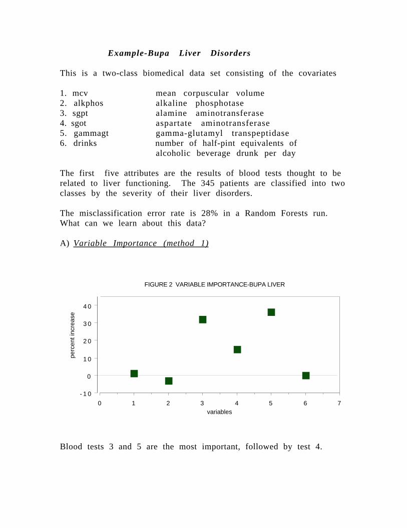
Example-Bupa Liver Disorders

This is a two-class biomedical data set consisting of the covariates

1. mcv mean corpuscular volume2. alkphos alkaline phosphotase3. sgpt alamine aminotransferase4. sgot aspartate aminotransferase5. gammagt gamma-glutamyl transpeptidase6. drinks number of half-pint equivalents of

alcoholic beverage drunk per day

The first five attributes are the results of blood tests thought to berelated to liver functioning. The 345 patients are classified into twoclasses by the severity of their liver disorders.

The misclassification error rate is 28% in a Random Forests run.What can we learn about this data?

A) Variable Importance (method 1)

- 1 0

0

1 0

2 0

3 0

4 0

perc

ent i

ncre

ase

0 1 2 3 4 5 6 7variables

FIGURE 2 VARIABLE IMPORTANCE-BUPA LIVER

Blood tests 3 and 5 are the most important, followed by test 4.

B) Clus te r ing

Using the proximity measure outputted by Random Forests tocluster, there are two class #2 clusters.

In each of these clusters, the average of each variable is computedand plotted:

FIGURE 3 CLUSTER VARIABLE AVERAGES

S omething interesting emerges. The class two subjects consist oftwo distinct groups: Those that have high scores on blood tests 3, 4,and 5 Those that have low scores on those tests. We will revisit thisexample below.

Scaling Coordinates

The proximities between cases n and k form a matrix {prox(n,k)}.From their definition, it is easy to show that this matrix issymmetric, positive definite and bounded above by 1, with thediagonal elements equal to 1. It follows that the values 1-prox(n,k)are squared distances in a Euclidean space of dimension not greaterthan the number of cases. For more background on scaling see"Multidimensional Scaling" by T.F. Cox and M.A. Cox

Let prox(n,-) be the average of prox(n,k) over the 2nd coordinate.and prox(-,-) the average over both coordinates. Then the matrix:

cv((n,k)=.5*(prox(n,k)-prox(n,-)-prox(k,-)+prox(- ,-))

is the matrix of inner products of the distances and is also positivedefinte symmetric. Let the eigenvalues of cv be λ (l) and theeigenvectors vl (n) Then the vectors

x(n) = ( λ (1)v1(n), λ (2)v2,(n), ...)

have squared distances between them equal to 1-prox(n,k). Werefer to the values of λ ( j)v j (n) as the jth scaling coordinate.

In metric scaling, the idea is to approximate the vectors x (n) by thefirst few scaling coordinates. This is done in random forests byextracting the number msdim of the largest eigenvalues andcorresponding eigenvectors of the cv matrix. The two dimensionalplots of the ith scaling coordinate vs. the jth often gives usefulinformation about the data. The most useful is usually the graph ofthe 2nd vs. the 1st.

We illustrate with three examples. The first is the graph of 2nd vs.1st scaling coordinates for the liver data

- . 25

- . 2

- . 15

- . 1

- . 05

0

.05

.1

.15

.2

- . 2 - . 15 - . 1 - . 05 0 .05 .1 .15 .2 .251st Scaling Coordinate

class 2

class 1

Metric Scaling Liver Data

The two arms of the class #2 data in this picture correspond to thetwo clusters found and discussed above.

The next example uses the microarray data. With 4682 variables, itis difficult to see how to cluster this data. Using proximities and thefirst two scaling coordinates gives this picture:

- . 2

- . 1

0

.1

.2

.3

.4

.5

.62n

d S

calin

g C

oord

inat

e

- . 5 - . 4 - . 3 - . 2 - . 1 0 .1 .2 .3 .41st Scaling Coordinate

class 3

class 2

class 1

Metric ScalingMicroarray Data

Random forests misclassifies one case. This case is represented bythe isolated point in the lower left hand corner of the plot.

The third example is glass data with 214 cases, 9 variables and 6classes. This data set has been extensively analyzed (see Patternrecognition and Neural Networkks-by B.D Ripley). Here is a plot ofthe 2nd vs. the 1st scaling coordinates.:

- . 4

- . 3

- . 2

- . 1

0

.1

.2

.3

.4

2nd

scal

ing

coor

dina

te

- . 5 - . 4 - . 3 - . 2 - . 1 0 .1 .21st scaling coordinate

class 6

class 5

class 4

class 3

class 2

class 1

Metric Scaling Glass data

None of the analyses to data have picked up this interesting andrevealing structure of the data--compare the plots in Ripley's book.

Outlier Location

Outliers are defined as cases having small proximities to all othercases. Since the data in some classes is more spread out thanothers, outlyingness is defined only with respect to other data in thesame class as the given case. To define a measure of outlyingness,we first compute, for a case n, the sum of the squares of prox(n,k)for all k in the same class as case n. Take the inverse of this sum--itwill be large if the proximities prox(n,k) from n to the other cases kin the same class are generally small. Denote this quantity byo u t ( n ) .

For all n in the same class, compute the median of the out(n), andthen the mean absolute deviation from the median. Subtract themedian from each out(n) and divide by the deviation to give anormalized measure of outlyingness. Yhe values less than zero areset to zero. Generally, a value above 10 is reason to suspect thecase of being outlying. Here is a graph of outlyingness for themicroarray data

- 2

0

2

4

6

8

1 0

1 2

1 4

outly

ingn

ess

0 1 0 2 0 3 0 4 0 5 0 6 0 7 0 8 0 9 0sequence number

class 3

class 2

class 1

Outlyingness MeasureMicroarray Data

There are two possible outliers--one is the first case in class 1, thesecond is the first case in class 2.

As a second example, we plot the outlyingness for the Pima Indianshepatitis data. This data set has 768 cases, 8 variables and 2 classes.It has been used often as an example in Machine Learning researchbut has been suspected of containing a number of outliers.

0

5

1 0

1 5

2 0

2 5

outly

ingn

ess

0 200 400 600 800sequence number

class 2

class 1

Outlyingness Measure Pima Data

If 10 is used as a cutoff point, there are 12 cases suspected of beingoutl iers.

Analyzing Unlabeled Data

Unlabeled date consists of N vectors {x(n)} in M dimensions. Usingthe iaddcl option in random forests, these vectors are assigned classlabel 1. Another set of N vectors is created and assigned class label2. The second synthetic set is created by independent samplingfrom the one-dimensional marginal distributions of the originalda ta .

For example, if the value of the mth coordinate of the original datafor the nth case is x(m,n), then a case in the synthetic data isconstructed as follows: its first coordinate is sampled at random

from the N values x(1,n), its second coordinate is sampled atrandom from the N values x(2,n), and so on. Thus the syntheticdata set can be considered to have the distribution of Mindependent variables where the distribution of the mth variable isthe same as the univariate distribution of the mth variable in theoriginal data.

When this two class data is run through random forests a highmisclassification rate--say over 40%, implies that there is not muchdependence structure in the original data. That is, that its structureis largely that of M independent variables--not a very interestingdistribution. But if there is a strong dependence structure betweenthe variables in the original data, the error rate will be low. In thissituation, the output of random forests can be used to learnsomething about the structure of the data. The following is anexample.

An Application to Chemical Spectra

Data graciously supplied by Merck consists of the first 468 spectralintensities in the spectrums of 764 compounds. The challengepresented by Merck was to find small cohesive groups of outlyingcases in this data. Using the iaddcl option, there was excellentseparation between the two classes, with an error rate of 0.5%,indicating strong dependencies in the original data.

We looked at outliers and generated this plot.

0

1

2

3

4

5ou

tlyin

gnes

s

0 100 200 300 400 500 600 700 800sequence numner

Outlyingness Measure Spectru Data

This plot gives no indication of outliers. But outliers must be fairlyisolated to show up in the outlier display. To search for outlyinggroups scaling coordinates were computed. The plot of the 2nd vs.the 1st is below:

- . 2

- . 15

- . 1

- . 05

0

.05

.1

.15

.2

.25

2nd

scal

ing

coor

dina

te

- . 25 - . 2 - . 15 - . 1 - . 05 0 .05 .1 .15 .2 .251st scaling coordinate

Metric ScalingSpecta Data

This shows, first, that the spectra fall into two main clusters. Thereis a possiblity of a small outlying group in the upper left handcorner. To get another picture, the 3rd scaling coordinate is plottedvs. the 1st.

- . 3

- . 25

- . 2

- . 15

- . 1

- . 05

0

.05

.1

.153r

d sc

alin

g co

ordi

ante

- . 25 - . 2 - . 15 - . 1 - . 05 0 .05 .1 .15 .2 .251st scaling coordinate

Metrc ScalingSpecta Data

The group in question is now in the lower left hand corner and itsseparation from the body of the spectra has become more apparent.

Saving Forests and Parameters

If the data set is large with many variables, a run growing 100 treesmay take awhile. If there is another set of data with the sameparameters except for sample size, the user may want to run this2nd set down the forest either to get classifications or to use thedata as a test set. In this case put isavef=1 and isavep=1.

When isavef is on, the variable values saved to file (which the usermust name-say 'forest55') are enough to reconstruct the forest. Ifirunf =1, then first, the new data are read in. Then the statementopen(1, file='forest55',status='old') runs the new data down thefores t .

If labelts is set =1, that implies that the new data has labels, and theprogram will output the error after each tree. If labelts=0, then thenew data has no class labels. But data must still be read in as

though there were values of the labels. Simply assign each label thevalue 1. As soon as these parameter values are filled in and the newdata read in, iut goes down the forest. If inewcl=1, then at the endof the run, all predicted class labels will be saved to a file.

The user knows ntest--the sample size of the data to run down thereconstituted forest. But may not remember the other values thatneed to be put in the parameter statement. However, if when doingthe initial run, isavep was put equal to 1 and a filename given inthe lines just before the end of the main program, then all theneeded parameters will be saved to the file as well as a textualdescription of up to 500 characters. The only thing that the userprovides is the file name and the textual description.

For these new runs modify the parameter statment as follows.1. all options should be turned off,2 set nsample0=1, ntest=sample size of the new data, and replacethe value of nrnodes by the value given in the parameter file.3. all other values stay the same as in the original run.

Parameters of the original run given by the file are nsample0,mdim,maxcat, nclass, jbt, nrnodes,the out-of-bag error rate, as well as theoriginal nsample0. The other parameters in the parameter statementsuch as mtry have no effect in the rerun.

If I have left anything out of this manual, let me know.(leo@stat.berkeley.edu). Please report bugs either to me orAdele Cutler (adele@sunfs.math.usu.edu)