manifolds: bird migration, hurricane · pdf fileto motivate further, consider the phenomenon...

arX

iv:1

405.

0803

v1 [

stat

.AP]

5 M

ay 2

014

The Annals of Applied Statistics

2014, Vol. 8, No. 1, 530–552DOI: 10.1214/13-AOAS701c© Institute of Mathematical Statistics, 2014

STATISTICAL ANALYSIS OF TRAJECTORIES ON RIEMANNIAN

MANIFOLDS: BIRD MIGRATION, HURRICANE TRACKING

AND VIDEO SURVEILLANCE

By Jingyong Su∗, Sebastian Kurtek†, Eric Klassen‡

and Anuj Srivastava‡

Texas Tech University∗, Ohio State University† and Florida StateUniversity‡

We consider the statistical analysis of trajectories on Rieman-nian manifolds that are observed under arbitrary temporal evolu-tions. Past methods rely on cross-sectional analysis, with the giventemporal registration, and consequently may lose the mean structureand artificially inflate observed variances. We introduce a quantitythat provides both a cost function for temporal registration and aproper distance for comparison of trajectories. This distance is usedto define statistical summaries, such as sample means and covari-ances, of synchronized trajectories and “Gaussian-type” models tocapture their variability at discrete times. It is invariant to identi-cal time-warpings (or temporal reparameterizations) of trajectories.This is based on a novel mathematical representation of trajectories,termed transported square-root vector field (TSRVF), and the L

2

norm on the space of TSRVFs. We illustrate this framework usingthree representative manifolds—S

2, SE(2) and shape space of pla-nar contours—involving both simulated and real data. In particular,we demonstrate: (1) improvements in mean structures and signifi-cant reductions in cross-sectional variances using real data sets, (2)statistical modeling for capturing variability in aligned trajectories,and (3) evaluating random trajectories under these models. Experi-mental results concern bird migration, hurricane tracking and videosurveillance.

1. Introduction. The need to summarize and model trajectories arises inmany statistical procedures. An important issue in this context is that trajec-tories are often observed at random times. If this temporal variability is notaccounted for in the analysis, then the resulting statistical summaries will

Received January 2013; revised November 2013.Key words and phrases. Riemannian manifold, time warping, variance reduction, tem-

poral trajectory, rate invariant, parallel transport.

This is an electronic reprint of the original article published by theInstitute of Mathematical Statistics in The Annals of Applied Statistics,2014, Vol. 8, No. 1, 530–552. This reprint differs from the original in paginationand typographic detail.

1

http://arxiv.org/abs/1405.0803v1

http://www.imstat.org/aoas/

http://dx.doi.org/10.1214/13-AOAS701

http://www.imstat.org

http://www.imstat.org

http://www.imstat.org/aoas/

http://dx.doi.org/10.1214/13-AOAS701

2 SU, KURTEK, KLASSEN AND SRIVASTAVA

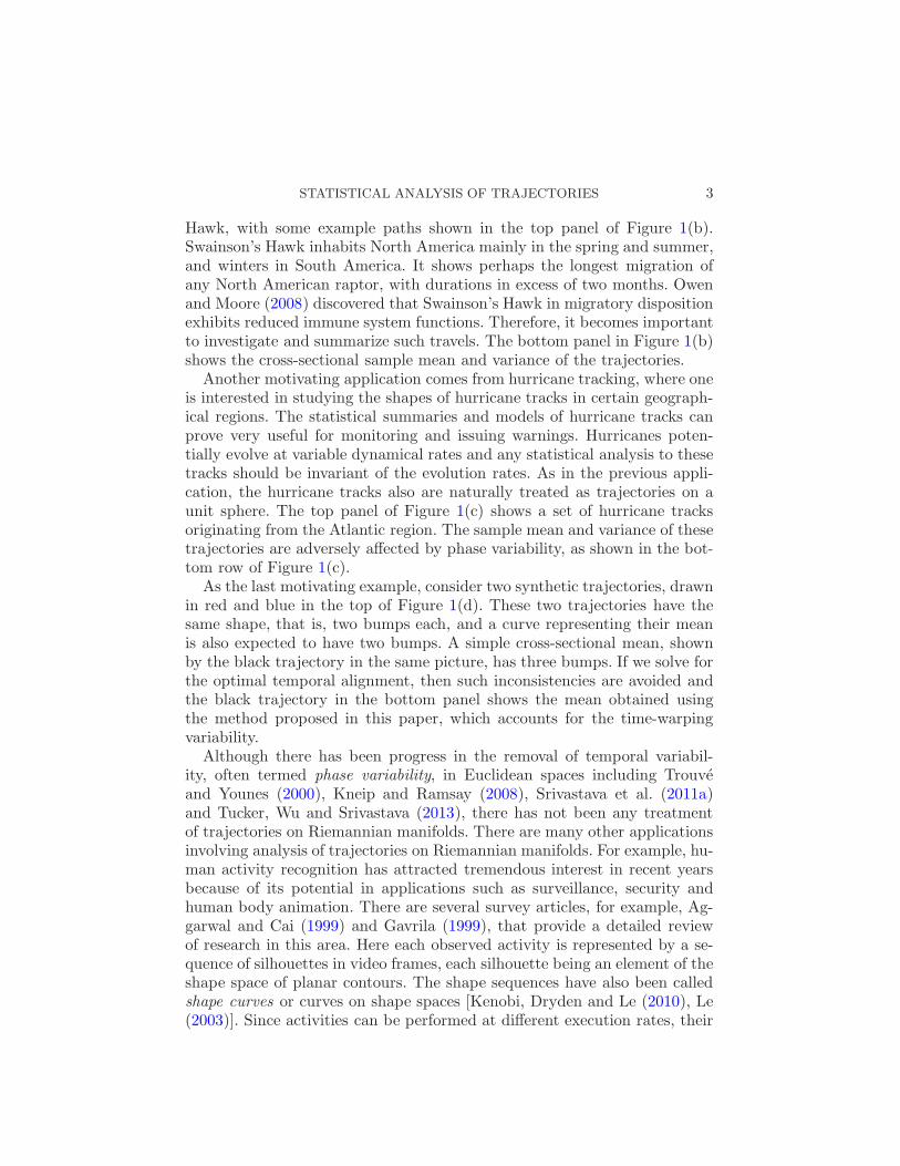
Fig. 1. Summary of trajectories on S2: (a) a simulated example; (b) bird migration paths;

(c) hurricane tracks; (d) cross-sectional mean of two trajectories without (top) and with(bottom) registration.

not be precise. The mean trajectory may not be representative of individualtrajectories and the cross-sectional variance will be artificially inflated. This,in turn, will greatly reduce the effectiveness of any subsequent modeling oranalysis based on the estimated mean and covariance. As a simple exampleconsider the trajectory on S

2 shown in the top panel of Figure 1(a). We sim-ulate a set of random, discrete observation times and generate observationsof this trajectory at these random times. These simulated trajectories areidentical in terms of the points traversed but their evolutions, or parame-terizations, are quite different. If we compute the cross-sectional mean andvariance, the results are shown in the bottom panel. We draw the samplemean trajectory in black and the sample variance at discrete times usingtangential ellipses. Not only is the mean fairly different from the originalcurve, the variance is purely due to randomness in observation times and issomewhat artificial. If we have observed the trajectory at fixed, synchronizedtimes, this problem would not exist.

To motivate further, consider the phenomenon of bird migration which isthe regular seasonal journey undertaken by many species of birds. There arevariabilities in migration trajectories, even within the same species, includingthe variability in their rates of travels. In other words, either birds can travelalong different paths or, even if they travel the same path, different birds (orsubgroups) may fly at different speed patterns along the path. This resultsin variability in observation times of migration paths for different birds andartificially inflates the cross-sectional variance in the data. Another issue isthat such trajectories are naturally studied as paths on a unit sphere whichis a nonlinear manifold. We will study the migration data for Swainson’s

STATISTICAL ANALYSIS OF TRAJECTORIES 3

Hawk, with some example paths shown in the top panel of Figure 1(b).Swainson’s Hawk inhabits North America mainly in the spring and summer,and winters in South America. It shows perhaps the longest migration ofany North American raptor, with durations in excess of two months. Owenand Moore (2008) discovered that Swainson’s Hawk in migratory dispositionexhibits reduced immune system functions. Therefore, it becomes importantto investigate and summarize such travels. The bottom panel in Figure 1(b)shows the cross-sectional sample mean and variance of the trajectories.

Another motivating application comes from hurricane tracking, where oneis interested in studying the shapes of hurricane tracks in certain geograph-ical regions. The statistical summaries and models of hurricane tracks canprove very useful for monitoring and issuing warnings. Hurricanes poten-tially evolve at variable dynamical rates and any statistical analysis to thesetracks should be invariant of the evolution rates. As in the previous appli-cation, the hurricane tracks also are naturally treated as trajectories on aunit sphere. The top panel of Figure 1(c) shows a set of hurricane tracksoriginating from the Atlantic region. The sample mean and variance of thesetrajectories are adversely affected by phase variability, as shown in the bot-tom row of Figure 1(c).

As the last motivating example, consider two synthetic trajectories, drawnin red and blue in the top of Figure 1(d). These two trajectories have thesame shape, that is, two bumps each, and a curve representing their meanis also expected to have two bumps. A simple cross-sectional mean, shownby the black trajectory in the same picture, has three bumps. If we solve forthe optimal temporal alignment, then such inconsistencies are avoided andthe black trajectory in the bottom panel shows the mean obtained usingthe method proposed in this paper, which accounts for the time-warpingvariability.

Although there has been progress in the removal of temporal variabil-ity, often termed phase variability, in Euclidean spaces including Trouveand Younes (2000), Kneip and Ramsay (2008), Srivastava et al. (2011a)and Tucker, Wu and Srivastava (2013), there has not been any treatmentof trajectories on Riemannian manifolds. There are many other applicationsinvolving analysis of trajectories on Riemannian manifolds. For example, hu-man activity recognition has attracted tremendous interest in recent yearsbecause of its potential in applications such as surveillance, security andhuman body animation. There are several survey articles, for example, Ag-garwal and Cai (1999) and Gavrila (1999), that provide a detailed reviewof research in this area. Here each observed activity is represented by a se-quence of silhouettes in video frames, each silhouette being an element of theshape space of planar contours. The shape sequences have also been calledshape curves or curves on shape spaces [Kenobi, Dryden and Le (2010), Le(2003)]. Since activities can be performed at different execution rates, their


corresponding shape curves will exhibit distinct evolution rates. Veeraragha-van et al. (2009) accounted for the time-warping variability but their methodhas some fundamental problems, as explained later. [Briefly, the method isbased on equation (2) which is not a proper distance. In fact, it is not evensymmetric.] Another motivating application is in pattern analysis of vehi-cle trajectories at a traffic intersection using surveillance videos, where theinstantaneous motion of a vehicle is denoted by the position and orienta-tion on the road. The movements of vehicles typically fall into predictablecategories—left turn, right turn, U turn, straight line—but the instanta-neous speeds can vary depending on the traffic. In order to classify thesemovements, one has to temporally align the trajectories, thus removing theeffects of travel speeds, and then compare them.

Now we describe the problem in mathematical terms. Let α : [0,1]→M ,where M is a Riemannian manifold, be a differentiable map; it denotesa trajectory on M . We will study such trajectories as elements of an ap-propriate subset of M [0,1]. Rather than observing a trajectory α directly,say, in the form of time observations α(t1), α(t2), . . . , we instead observethe time-warped trajectory α(γ(t1)), α(γ(t2)), . . . , where γ : [0,1]→ [0,1] isan unknown time-warping function (a function with certain constraints de-scribed later) that governs the rate of evolution. The mean and variance of{α1(t), α2(t), . . . , αn(t)} for any t, where n is the number of observed tra-jectories, are termed the cross-sectional mean and variance at that t. If weuse the observed samples {αi(γi(t)), i = 1,2, . . . , n} for analysis, the cross-sectional variance is inflated due to random γi. Our hypothesis is that thisproblem can be mitigated by temporally registering the trajectories. Thus,we are interested in the following four tasks:

1. Temporal registration: This is a process of establishing a one-to-one corre-spondence between points along multiple trajectories. That is, given anyn trajectories, say, α1, α2, . . . , αn, we are interested in finding functionsγ1, γ2, . . . , γn such that the points αi(γi(t)) are matched optimally for allt.

2. Metric-based comparisons: We want to develop a metric that is invariantto different evolution rates of trajectories. Specifically, we want to definea distance d(·, ·) such that for arbitrary evolution functions γ1, γ2 andarbitrary trajectories α1 and α2, we have d(α1, α2) = d(α1 ◦ γ1, α2 ◦ γ2).

3. Statistical summary : The main use of this metric will be in defining andcomputing a (Karcher) mean trajectory µ(t) and a cross-sectional vari-ance function ρ(t), associated with any given set of trajectories. Thereason for performing registration is to reduce the cross-sectional vari-ance that is artificially introduced in the data due to random observationtimes. The reduction in variance is quantified using ρ.


4. Statistical modeling and evaluation: We will use the estimated mean andcovariance of registered trajectories to define a “Gaussian-type” modelon random trajectories. This model will then be used to evaluate p-valuesassociated with new trajectories. Here the p-value implies the proportionof trajectories with smaller density than the current trajectory under thegiven model.

For performing comparison and summarization of trajectories, we need ametric and, at first, we consider a more conventional solution. Since M is aRiemannian manifold, we have a natural distance dm between points on M .Using dm, one can compare any two trajectories: α1, α2 : [0,1]→M , as

dx(α1, α2) =

∫ 1

0dm(α1(t), α2(t))dt.(1)

Although this quantity represents a natural extension of dm from M toM [0,1], it suffers from the problem that dx(α1, α2) 6= dx(α1 ◦ γ1, α2 ◦ γ2) ingeneral. It is not preserved even when the same γ is applied to both trajec-tories, that is, dx(α1, α2) 6= dx(α1 ◦ γ,α2 ◦ γ) in general. If we have equalityin the last case, for all γ, then we can develop a fully invariant distance anduse it to properly register trajectories, as described later. So, the failure tohave this equality is a key issue that forces us to look for other solutions insituations where trajectories are observed at random temporal evolutions.When a trajectory α is observed as α ◦ γ, for an arbitrary temporal re-parameterization γ, we call this perturbation compositional noise. In theseterms, dx is not useful in comparing trajectories observed under composi-tional noise.

Our goal is to take time-warping into account, derive a warping-invariantmetric, and generate statistical summaries (sample mean, covariance, etc.)for trajectories on a set M . The fact that M is a Riemannian manifoldpresents a formidable challenge in developing a comprehensive framework.But this is not the only challenge. To clarify, how has this registration andanalysis problem been handled for trajectories in Euclidean spaces? In caseM = R, that is, if one is interested in registration and modeling of real-valued functions under random time-warpings, the problem has been stud-ied by many authors, including Srivastava et al. (2011a), Liu and Muller(2004), Kneip and Ramsay (2008) and Tucker, Wu and Srivastava (2013).In case M =R

2, where the problem involves registration and shape analysisof planar curves, the solution is discussed in Michor and Mumford (2007),Younes et al. (2008), Shah (2008) and Sundaramoorthi et al. (2011). Srivas-tava et al. (2011b) proposed a solution that applies to curves in arbitrary R

n.One can also draw solutions from problems in image registration where 2Dand 3D images are registered to each other using a spatial warping insteadof a temporal warping [see, e.g., LDDMM technique, Beg et al. (2005)]. A


majority of the existing methods in Euclidean spaces formulate an objectivefunction of the type

minγ

(∫ 1

0|α1(t)−α2(γ(t))|2 dt+ λR(γ)

)

,

where | · | is the Euclidean norm, R is a regularization term on the warpingfunction γ, and λ > 0 is a constant. In the case of a Riemannian manifold,one can modify the first term to obtain

minγ

(∫ 1

0dm(α1(t), α2(γ(t)))

2 dt+ λR(γ)

)

,(2)

where dm(·, ·) is the geodesic distance on the manifold. The main problemwith this procedure is that (a) it is not symmetric, that is, the registration ofα1 to α2 is not the same as that of α2 to α1, as pointed out by Christensenand Johnson (2001), among others, and (b) the minimum value is not aproper distance, so it cannot be used to compare trajectories. This sumsup the fundamental dilemma in trajectory analysis—equation (1) provides ametric between trajectories but does not perform registration, while equation(2) performs registration but is not a metric.

Another potential approach is to map trajectories onto a vector space, forexample, the tangent space at a point, using the inverse exponential map,and then compare the mapped trajectories using the Euclidean solutions inthe vector space. While this idea is feasible, the results may not be consistentsince the inverse exponential map is a local and highly nonlinear operator.For example, on a sphere, under stereographic map two points near thesouth pole will map to two distant points in the tangent space at the northpole, and their distance will be highly distorted. In contrast, the solutionproposed here transports vector fields associated with trajectories, ratherthan trajectories themselves, into a standard tangent space and this providesa more stable alternative.

We would like an objective function for alignment that (a) is a properdistance, that is, it is symmetric, positive definite and satisfies the triangleinequality, (b) is invariant to simultaneous warping of two trajectories by thesame warping function, and (c) leads to minimal cross-sectional variance forsample trajectories. For real-valued functions, a Riemannian framework hasalready been presented in Kurtek, Wu and Srivastava (2011) and Srivastavaet al. (2011a), but to our knowledge this framework has not been generalizedto manifolds.

In this paper we develop a framework for automated registration of mul-tiple trajectories and obtain improvements in statistical summaries of time-warped trajectories on Riemannian manifolds. This framework is based on anovel mathematical representation called the transported square-root vector


field (TSRVF) and the L2 norm between TSRVFs. The setup satisfies the

invariance property mentioned earlier, that is, an identical time-warping ofTSRVFs representing two trajectories preserves the L

2 norm of their dif-ference and, therefore, this difference is used to define a warping-invariantdistance between trajectories. The resulting distance is found useful in reg-istration, comparison and summarization of trajectories on manifolds. Toillustrate these ideas, we take three manifolds, S

2, SE(2) and the shapespace of planar closed curves, and provide simulated and real examples. Ourpaper can also be viewed as an extension, albeit not a trivial one, of thework of Kurtek, Wu and Srivastava (2011) and Srivastava et al. (2011a)from M =R to Riemannian manifolds.

The paper is organized as follows. In Section 2 we introduce a generalmathematical framework for analyzing trajectories on Riemannian mani-folds and demonstrate the use of this framework in registration, compari-son, summarization, modeling and evaluation. We also provide algorithmsfor performing these tasks. In Section 3 we specialize this framework to S

2

and consider two applications. In Section 4 we apply it to pattern anal-ysis of vehicle trajectories on SE(2). In Section 5 we provide details fortime-warping invariant analysis of trajectories on the shape space of planarclosed curves, with applications to activity recognition.

2. Mathematical framework. Let α denote a smooth trajectory on aRiemannian manifold M endowed with a Riemannian metric 〈·, ·〉. Let Mdenote the set of all such trajectories: M = {α : [0,1] → M |α is smooth}.Also, define Γ to be the set of all orientation preserving diffeomorphisms of[0,1] :Γ = {γ : [0,1] → [0,1]|γ(0) = 0, γ(1) = 1, γ is a diffeomorphism}. Notethat Γ forms a group under the composition operation. If α is a trajectoryon M , then α ◦ γ is a trajectory that follows the same sequence of pointsas α but at the evolution rate governed by γ. More technically, the group Γacts on M according to (α,γ) = α ◦ γ.

Given two smooth trajectories α1, α2 ∈ M, we want to register pointsalong the trajectories and compute a time-warping invariant distance be-tween them. As mentioned earlier, the quantity given in equation (2) wouldbe a natural choice for this purpose, but it fails for several reasons, includingthe fact that it is not symmetric. Fundamentally, this and other quantitiesused in previous literature are not appropriate for solving the registrationproblem because they are not measuring registration in the first place. Tohighlight this issue, take the registration of points between the pair (α1, α2)and the pair (α1 ◦ γ,α2 ◦ γ), for any γ ∈ Γ. It can be seen that the pairs(α1, α2) and (α1 ◦ γ,α2 ◦ γ) have exactly the same registration of points.In fact, any identical time-warping of two trajectories does not change theregistration of points between them. But the quantities given in equations


(1) and (2) provide different values for these pairs, despite the same regis-tration. Hence, they are not good measures of registration. We emphasizethat the invariance under identical time-warping is a key property neededin the desired framework.

We introduce a new representation of trajectories that will be used tocompare and register them. We assume that for any two points p, q ∈M , wehave an expression for parallel transporting any vector v ∈ Tp(M) along theshortest geodesic from p to q, denoted by (v)p→q. As long as p and q do notfall in the cut loci of each other, the geodesic between them is unique andthe parallel transport is well defined. The measure of the set of cut locus onthe manifolds of our interest is typically zero. So, the practical implicationsof this limitation are negligible. Let c be a point in M that we designateas a reference point. We assume that none of the observed trajectories passthrough the cut locus of c to avoid the problem mentioned above.

Definition 1. For any smooth trajectory α ∈M, the transported square-root vector field (TSRVF) is a parallel transport of a scaled velocity vectorfield of α to a reference point c ∈M according to

hα(t) =α(t)α(t)→c√

|α(t)|∈ Tc(M),

where | · | denotes the norm related to the Riemannian metric on M .

Since α is smooth, so is the vector field hα. Let H ⊂ Tc(M)[0,1] be theset of smooth curves in Tc(M) obtained as TSRVFs of trajectories in M ,H = {hα|α ∈M}. If M = R

n with the Euclidean metric, then h is exactlythe square-root velocity function defined in Srivastava et al. (2011b).

The choice of the reference point c used in Definition 1 is important andcan affect the results. The choice typically depends on the application, thedata and the manifold under study. In case all the trajectories pass througha point or pass close to a point, then that point is a natural candidate forc. This would be true, for example, in the case of hurricane tracks, if weare focused on all hurricanes starting from the same region. Another re-mark is that instead of parallel transporting of scaled velocity vectors alonggeodesics, one can transport them along trajectories themselves, as was doneby Jupp and Kent (1987), but that requires c to be a common point of alltrajectories. While the choice of c can, in principle, affect distances, our ex-periments suggest that the results of registration, distance-based clusteringand classification are quite stable with respect to this choice. An example ispresented later in Figure 2.

We represent a trajectory α ∈M with the pair (α(0), hα) ∈M ×H. Giventhis representation, we can reconstruct the path, an element ofM, as follows.


For any time t, let Vt be a time-varying tangent vector-field on M obtainedby parallel transporting hα(t) over M [except for the cut locus of α(t)], thatis, for any p ∈M , Vp(t) = (hα(t))c→p. Then, define an integral curve β such

that β(t) = |Vβ(t)(t)|Vβ(t)(t) with the starting point β(0) = α(0) ∈M . Thisresulting curve β will be exactly the same as the original curve α.

The starting points of different curves can be compared using the Rieman-nian distance dm on M . However, these points do not play an important rolein the alignment of trajectories since they are already assumed to be matchedto each other. Therefore, the main focus of analysis, in terms of alignmentand comparison, is on TSRVFs. Since a TSRVF is a path in Tc(M), one canuse the L

2 norm to compare such paths.

Definition 2. Let α1 and α2 be two smooth trajectories on M and lethα1 and hα2 be the corresponding TSRVFs. The distance between them is

dh(hα1 , hα2) =

(∫ 1

0|hα1(t)− hα2(t)|2 dt

)1/2

.

The distance dh, being the standard L2 norm, satisfies symmetry, posi-

tive definiteness and triangle inequality. Also, due to the invertibility of themapping from M to M ×H, one can use dh (along with dm) to define adistance on M. The main motivation of this setup—TSRVF representationand L

2 norm—comes from the following fact. If a trajectory α is warped byγ, to result in α ◦ γ, the TSRVF of α ◦ γ is given by

hα◦γ(t) =(α(γ(t))γ(t))α(γ(t))→c

√

|α(γ(t))γ(t)|=

(α(γ(t)))α(γ(t))→c

√

γ(t)√

|α(γ(t))|

= hα(γ(t))√

γ(t),

which is also denoted as (hα, γ)(t). We will often write (hα, γ) to denotehα◦γ . As stated earlier, we need a distance for registration that is invariantto identical time-warpings of trajectories. Next, we show that dh satisfiesthis property.

Theorem 1. For any α1, α2 ∈M and γ ∈ Γ, the distance dh satisfiesdh(hα1◦γ , hα2◦γ) = dh(hα1 , hα2). In geometric terms, this implies that the ac-

tion of Γ on H under the L2 metric is by isometries.

The proof is given below:

dh(hα1◦γ , hα2◦γ) =

(∫ 1

0|hα1(γ(t))

√

γ(t)− hα2(γ(t))√

γ(t)|2 dt)1/2

=

(∫ 1

0|hα1(s)− hα2(s)|2 ds

)1/2

= dh(hα1 , hα2),


where s= γ(t).Next we define a quantity that can be used as a distance between trajec-

tories while being invariant to their temporal variability. To set up this def-inition, we first introduce an equivalence relation between trajectories. Forany two trajectories α1 and α2, we define them to be equivalent, α1 ∼ α2,when:

1. α1(0) = α2(0), and2. there exists a sequence {γk} ∈ Γ such that limk→∞ h(α1◦γk) = hα2 under

the L2 metric.

In other words, any two trajectories are equivalent if they have the samestarting point and the TSRVF of one can be time-warped into the TSRVFof the other using a sequence of warpings. It can be easily checked that ∼forms an equivalence relation on H (and, correspondingly, M).

Since we want our distance to be invariant to time-warpings of trajecto-ries, we wish to compare trajectories by comparing their equivalence classes.Thus, our next step is to inherit the distance dh to the set of such equivalenceclasses. Toward this goal, we introduce the set Γ as the set of all nondecreas-ing, absolutely continuous functions γ : [0,1]→ [0,1] such that γ(0) = 0 andγ(1) = 1. This set Γ is a semigroup with the composition operation (it isnot a group because the elements do not have inverses). The group Γ isa subset of Γ. The elements of Γ warp the time axis of trajectories in Min the same way as elements of Γ, except they allow certain singularities.For a TSRVF hα ∈ H, its equivalence class, or orbit under Γ, is given by[hα] = {(hα, γ)|hα ∈H, γ ∈ Γ}.

It can be shown that the orbits under Γ are exactly the same as theclosures of the orbits of Γ, defined as [hα]0 = {(hα, γ)|γ ∈ Γ}, as long as αhas nonvanishing derivatives almost everywhere. (The last condition is notrestrictive since we can always re-parameterize α by the arc-length.) Theclosure is with respect to the L

2 metric on H. Please refer to Robinson(2012) for a detailed description of a similar construction for trajectories inR.

Now we define the quantity that will serve both as the cost functionfor registration and distance for comparison. This quantity is essentially dhmeasured between equivalence classes.

Definition 3. The distance ds on H/∼ (or M/∼) is the shortest dhdistance between equivalence classes in H, given as

ds([hα1 ], [hα2 ])

= infγ1,γ2∈Γ

dh((hα1 , γ1), (hα2 , γ2))(3)

= infγ1,γ2∈Γ

(∫ 1

0|hα1(γ1(t))

√

γ1(t)− hα2(γ2(t))√

γ2(t)|2 dt)1/2

.


Theorem 2. The distance ds is a proper distance on H/∼.

Proof. The symmetry of ds comes directly from the symmetry of dh.For positive definiteness, we need to show that ds([hα1 ], [hα2 ]) = 0⇒ [hα1 ] =[hα2 ]. Suppose that ds([hα1 ], [hα2 ]) = 0, by definition, it then follows imme-diately that for all ε > 0, there exists a γ ∈ Γ such that dh(hα1 , (hα2 , γ))< ε.From this, it follows that hα1 is in the orbit hα2 . Since we are assuming thatorbits are closed, it follows that hα1 ∈ [hα2 ], so [hα1 ] = [hα2 ].

To establish the triangle inequality, we need to prove

ds([hα1 ], [hα3 ])≤ ds([hα1 ], [hα2 ]) + ds([hα2 ], [hα3 ])

for any hα1 , hα2 , hα3 ∈H. For a contradiction, suppose

ds([hα1 ], [hα3 ])> ds([hα1 ], [hα2 ]) + d([hα2 ], [hα3 ]).

Let

ε= 13(ds([hα1 ], [hα3 ])− ds([hα1 ], [hα2 ])− ds([hα2 ], [hα3 ])).

By our supposition, ε > 0. From the definition of ε, it follows that

ds([hα1 ], [hα3 ]) = ds([hα1 ], [hα2 ]) + ds([hα2 ], [hα3 ]) + 3ε.

By the definition of ds, we can choose γ1, γ2 ∈ Γ, such that

dh((hα1 , γ1), hα2)≤ ds([hα1 ], [hα2 ]) + ε

and

dh(hα2 , (hα3 , γ2))≤ ds([hα2 ], [hα3 ]) + ε.

Now, by the triangle inequality for dh, we know that

dh((hα1 , γ1), (hα3 , γ2))≤ dh((hα1 , γ1), hα2) + dh(hα2 , (hα3 , γ2))

≤ ds([hα1 ], [hα2 ]) + ds([hα2 ], [hα3 ]) + 2ε.

It follows that

ds([hα1 ], [hα3 ])≤ ds([hα1 ], [hα2 ]) + ds([hα2 ], [hα3 ]) + 2ε.

But this contradicts the fact that

ds([hα1 ], [hα3 ]) = ds([hα1 ], [hα1 ]) + ds([hα2 ], [hα3 ]) + 3ε.

Hence, our supposition that

ds([hα1 ], [hα3 ])> ds([hα1 ], [hα2 ]) + ds([hα2 ], [hα3 ])

must be false. The triangle inequality follows. �


Now, since Γ is dense in Γ, for any δ > 0, there exists a γ∗ such that

|dh(hα1 , hα2◦γ∗)− ds([hα1 ], [hα2 ])|< δ.(4)

This γ∗ may not be unique but any such γ∗ is sufficient for our purpose.Furthermore, since γ∗ ∈ Γ, it has an inverse that can be used in furtheranalysis. The minimization over Γ in equation (4) is performed in practiceusing the dynamic programming (DP) algorithm [Bertsekas (2007)]. Hereone samples the interval [0,1] using T discrete points and then restricts toonly piecewise linear γ’s that pass through that T × T grid. The search forthe optimal trajectory on this grid is accomplished in O(T 2) steps.

2.1. Metric-based comparison of trajectories. Our goal of warping-invariantcomparison of trajectories is achieved using ds. For any γ1, γ2 ∈ Γ and α1,α2 ∈M, we have

[hα1◦γ1 ] = [hα1 ], [hα2◦γ2 ] = [hα2 ]

and, therefore, we get ds([hα1◦γ1 ], [hα2◦γ2 ]) = ds([hα1 ], [hα2 ]). Examples ofthis metric are presented later.

2.2. Pairwise temporal registration of trajectories. The next goal is toperform registration of points along trajectories. Let our approximation tothe optimal warping be as defined in equation (4). This allows for the reg-istration between α1 and α2, in that the point α1(t) on the first trajectoryis optimally matched to the point α2(γ

∗(t)) on the second trajectory.If we compare equation (3) with equation (2), we see the advantages

of the proposed framework. Both equations present a registration problembetween α1 and α2, but only the minimum value resulting from equation (3)is a proper distance. Also, in equation (2) we have two separate terms formatching and regularization, with an arbitrary weight λ, but in equation (3)the two terms have been merged into a single natural form. Recall that thechange in TSRVF h due to the time-warping of α by γ is given by (h,γ) =(h ◦ γ)√γ, and the distance ds is based on these warped TSRVFs. The term√γ provides an intrinsic regularization on γ in the matching process. It

provides an elastic penalty against excessive warping since γ becomes largeat those places. Lastly, the optimal registration in equation (3) remains thesame if we change the order of the input functions. That is, the registrationprocess is inverse consistent.

2.3. Summarization and registration of multiple trajectories. An addi-tional advantage of this framework is that one can compute an average ofseveral trajectories and use it as a template for future classification. Fur-thermore, this template can be used for registering multiple trajectories. We


use the notion of the Karcher mean to define and compute average trajecto-ries. Given a set of sample trajectories α1, . . . , αn on M , we represent themusing the corresponding pairs (α1(0), hα1), (α2(0), hα2), . . . , (αn(0), hαn). Wecompute the Karcher means of each component in their respective spaces:(1) the Karcher mean of αi(0) is computed with respect to dm in M , and(2) the Karcher mean of hαi

with respect to ds in H/∼. The latter Karchermean is defined as

hµ = argmin[hα]∈H/∼

n∑

i=1

ds([hα], [hαi])2.

Note that [hµ] is an equivalence class of trajectories and one can select anyelement of this mean class to help in the alignment of multiple trajectories.The standard algorithm to compute the Karcher mean proposed by Le andKume (2000) is adapted to this problem as follows:

Algorithm 1 (Karcher mean of multiple trajectories). Compute theKarcher mean of {αi(0)} and set it to be µ(0).

1. Initialization step: select µ to be one of the original trajectories and com-pute its TSRVF hµ.

2. Align each hαi, i= 1, . . . , n, to hµ according to equation (4). That is, solve

for γ∗i using the DP algorithm and set αi = αi ◦ γ∗i .3. Compute TSRVFs of the warped trajectories, hαi

, i= 1,2, . . . , n, and up-date hµ as a curve in Tc(M) according to hµ(t) =

1n

∑ni=1 hαi

(t).4. Define µ to be the integral curve associated with a time-varying vector

field on M generated using hµ, that is, dµ(t)dt = |hµ(t)|(hµ)(t)c→µ(t), and

the initial condition µ(0).5. Compute E =

∑ni=1 ds([hµ], [hαi

])2 =∑n

i=1 dh(hµ, hαi)2 and check for con-

vergence. If not converged, return to step 2.

It can be shown that the cost function decreases iteratively and, as zerois a natural lower bound,

∑ni=1 ds([hµ], [hαi

])2 will always converge. Thisalgorithm provides two sets of outputs: an average trajectory denoted bythe final µ and the set of aligned trajectories αi. Therefore, this solves theproblem of aligning multiple trajectories too.

For computing and analyzing the second and higher moments of a sampletrajectory, the tangent space Tµ(t)(M), for t ∈ [0,1], is used. This is con-venient because it is a vector space and one can apply more traditionalmethods here. First, for each aligned trajectory αi(t) at time t, the vectorvi(t) ∈ Tµ(t)(M) is computed such that a geodesic that goes from µ(t) to αi(t)in unit time has the initial velocity vi(t). This is also called the shooting vec-

tor from µ(t) to αi(t). Let K(t) be the sample covariance matrix of all shoot-ing vectors from µ(t)’s to αi(t)’s. The sample Karcher covariance at time t isgiven by K(t) = 1

n−1

∑ni=1 vi(t)vi(t)

T , with the trace ρ(t) = trace(K(t)). This


ρ(t) represents a quantification of the cross-sectional variance, as a functionof t, and can be used to study the level of alignment of trajectories. Also,for capturing the essential variability in the data, one can perform PrincipalComponent Analysis (PCA) of the shooting vectors. The basic idea is to

compute the Singular Value Decomposition (SVD) K(t) = U(t)Σ(t)UT (t),where U(t) is an orthogonal matrix and Σ(t) is the diagonal matrix of sin-gular values. Assuming that the entries along the diagonal in Σ(t) are orga-nized in a nonincreasing order, the functions U1(t),U2(t), . . . represent thedominant directions of variability in the data.

2.4. Modeling and evaluation of trajectories. An important use of meansand covariances of trajectories is in devising probability models for capturingthe observed statistical variability, and for using these models in evaluatingp-values of future observations. By p-values we mean the proportion of ran-dom trajectories that will have lower probability density under a given modelwhen compared to the test trajectory. Several models are possible in this sit-uation, but since our main focus is on temporal registration of trajectories,we will choose a simple model to demonstrate our ideas. After the registra-tion, we treat a trajectory α as a discrete-time process, composed ofm pointsas {α(t1), α(t2), . . . , α(tm)}, for a fixed partition {0 = t1, t2, . . . , tm = 1} of[0,1]. Given the mean and the covariance at each tj , we model the pointsα(tj) ∈M,j = 1,2, . . . ,m independently, and obtain the joint density by tak-ing the product. The difficulty in this step comes from the fact that M is anonlinear manifold but one can use the tangent space Tµ(tj )(M), instead, toimpose a probability model since this is a vector space. We impose a mul-tivariate normal density on the tangent vector v(tj) = exp−1

µ(tj )(α(tj)), with

mean zero and variance given by K(tj) (as defined above). It is analogousto the model of additive white Gaussian noise when M = R. Then, for anytrajectory α, one can compute a joint probability of the full trajectory as

P (α) =∏m

j=1 f(α(tj)) ≡∏m

j=1N(v(tj); 0, K(tj)). This model is potentially

useful for many situations: (1) It can be used to simulate new trajectories

via random sampling. Given {(µ(tj), K(tj))|t ∈ [0,1]}, we can simulate thetangent vectors and compute the corresponding trajectory points α(tj), forthe desired tj . (2) Given a trajectory, we evaluate its p-value under the im-posed model. This measures how likely is the occurrence of the trajectory bychance assuming the null hypothesis H0, where H0 represents that imposedmodel.

Since we are interested in studying the effects of temporal registration,we demonstrate these ideas with the following experiment. We compute p-values of trajectories using the parametric bootstrap under two situations:without registration and with registration. In each situation, we first take aset of trajectories as the training set and estimate the mean and covariance at


each discrete time, and then impose a “Gaussian-type” model on the tangentspaces of M at the mean values at those times. This becomes the imposedmodel H0. The evaluation of p-values requires Monte Carlo sampling. Wegenerate a large number, say, N = 10,000, of trajectories from the model,denoted as Xi, i= 1,2, . . . ,N . Then we compute the proportion that are lesslikely than our test trajectory and denote it as p(α) = 1

N

∑Ni=1 1[P (Xi)<P (α)].

In the following sections we consider three examples of M and presentexperimental results to validate our framework.

3. Trajectories on S2. Statistical methods for unit vectors in three-dimensio-

nal space have been studied extensively in directional statistics [Mardiaand Jupp (2000)]. In the landmark-based shape analysis of objects, includ-ing Dryden and Mardia (1998), Jupp and Kent (1987) and Kume, Dry-den and Le (2007), where 2D objects are represented by configurations ofsalient points or landmarks, the set of all such configurations after remov-ing translation and scale is a real sphere S

2n−3 (for configurations withn landmarks). To illustrate this framework, in a simple setting, we startwith M = S

2, with the standard Euclidean Riemannian metric. For any twopoints p, q ∈ S

2 (p 6=−q) and a tangent vector v ∈ Tp(S2), the parallel trans-

port (v)p→q along the shortest geodesic (i.e., great circle) from p to q is given

by v− 2〈v,q〉|p+q|2

(p+ q).

Registration of trajectories: As mentioned earlier, for any two trajectorieson S

2, we use their TSRVFs and DP algorithm in equation (4) to find theoptimal registration between them. In Figure 2 we show one example of reg-istering such trajectories. The parameterization of trajectories is displayedusing colors. In the top row, the left column shows the trajectories α1 andα2, the middle column shows α1 and α2 ◦ γ∗ and the right column shows γ∗

using c= [0,0,1]. The correspondences between the two trajectories are de-picted by black lines connecting points along them. Due to the optimizationof γ in equation (4), the dh value between them reduces from 1.67 to 0.36and the correspondences become more natural after the alignment. We alsoconsider different choices of c (c = [0,0,−1], [−1,0,0], [0,1,0]). In all casesthe registration results are very close, as shown in the bottom row.

In the following, we consider two specific applications, bird migration andhurricane tracks, and show how the cross-sectional variance of the meantrajectories is reduced by registration. For both applications, we use themean of the starting points of the trajectories as the reference point c inDefinition 1.

Bird migration data: This data set has 35 migration trajectories of Swain-son’s Hawk, observed during the period 1995 to 1997, each having geo-graphic coordinates measured at some random times. Several sample paths


Fig. 2. Registration of trajectories on S2.

are shown at the top row in Figure 3(a). In the bottom panel of Figure 3(a),we show the optimal warping functions {γ∗i } used in aligning them and thisclearly highlights a significant temporal variation present in the data. In

Fig. 3. Swainson’s Hawk migration: (a) {αi} (top) and {γ∗i } (bottom); (b) µ and ρ

without registration; (c) µ and ρ with registration.


Fig. 4. ρ (1st row) and p-values (2nd row) for each trajectory without (red) and with(blue) registration.

Figure 3(b) and (c), we show the Karcher mean µ and the cross-sectional

variance ρ without and with registration, respectively. In the top row, µ

is displayed using colors, where red areas correspond to higher ρ value. In

the bottom row, the principal modes of variation are displayed by ellipses

on tangent spaces. We use the first and second principal tangential direc-

tions as the major and minor axes of ellipses, and the corresponding singular

values as their sizes. We observe that (1) the mean after registration bet-

ter preserves the shapes of trajectories, and (2) the variance ellipses before

registration have their major axes along the trajectory while the ellipses

after registration exhibit a smaller, actual variability in the data. Most of

the variability after registration is limited to the top end where the origi-

nal trajectories indeed have differences. The top row of Figure 4(a) shows a

decrease in the function ρ due to the registration.

Next we construct a “Gaussian-type” model for these trajectories using

estimated summaries for two cases (with and without temporal registration),

as described previously, and compute p-values of individual trajectories using

Monte Carlo simulation. The results are shown in the bottom of Figure 4(a),

where we note a general increase in the p-values for the original trajectories

after the alignment. This is attributed to a reduced variance in the model

due to temporal alignment and the resulting movement of individual samples

closer to the mean values.


Fig. 5. Summary of hurricane tracks without and with temporal registration.

Hurricane tracks: We choose two subsets of Atlantic Tracks File 1851-2011, available on the National Hurricane Center website.1 The first subsethas 10 tracks and another has 7 tracks, with observations at six-hour sep-aration. In Figure 5 we show the data, their Karcher mean and variancewithout and with registration for each subset. The decrease in the value ofρ is shown in the top of Figure 4(b) and (c). Although the decrease here isnot as large as the previous example, we observe about 20% reduction in ρon average due to registration. In the bottom plots of Figure 4(b) and (c), itis also seen that there is a general increase of the p-values after registration,although they decreased in a few cases. This is because those trajectoriesare closer to the mean without registration.

4. Vehicle trajectories on SE(2). Here we study the problem of classify-ing vehicle trajectories into broad motion patterns using data obtained fromtraffic videos. While the general motion of a vehicle at a traffic intersection ispredicable—left turn, right turn, U turn or straight line—the travel speedsof vehicles may be different in distinct instances due to traffic variations.Since we are interested in tracking position and orientation of a vehicle, weconsider individual tracks as parameterized trajectories on SE(2), which isa semidirect product of SO(2) and R

2, that is, SE(2) = SO(2)⋊R2. For the

rotation component O ∈ SO(2) and tangent vectors X1,X2 ∈ TO(SO(2)), the

1http://www.nhc.noaa.gov/pastall.shtml.

http://www.nhc.noaa.gov/pastall.shtml


Fig. 6. (a): Real trajectories in SE(2) obtained from a traffic video. (b): Trajectoriesused for clustering.

standard Riemannian metric is given by 〈X1,X2〉= trace(XT1 X2), while we

use the Euclidean metric for R2. We choose the rotation component of c asthe identity matrix and the translation component as [0,0]. We found thatthe results of registration, clustering and classification are quite stable withrespect to different choices of c. For a tangent vector W ∈ TO(SO(2)), theparallel transport of W from O to I2×2 is OTW . The formulae for the R

2

component are standard.

Registration of trajectories: The data for this experiment comes from traf-fic videos available at the Image Sequence Server website.2 In Figure 6(a)we show an example trajectory for each of the three classes: right turn (firstpanel), left turn (second panel), and straight line (third panel). In this smallexperiment, the total data includes 14 trajectories with 5 trajectories cor-

Fig. 7. Registration of trajectories on SE(2).

2http://i21www.ira.uka.de/image_sequences/.

http://i21www.ira.uka.de/image_sequences/


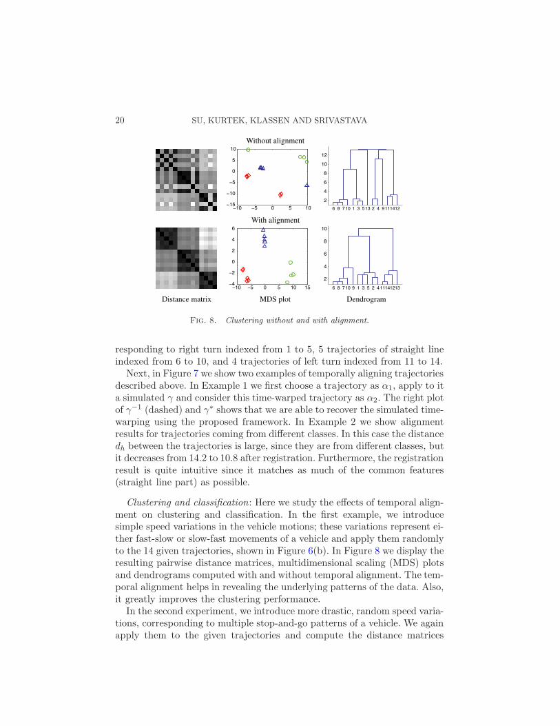
Fig. 8. Clustering without and with alignment.

responding to right turn indexed from 1 to 5, 5 trajectories of straight lineindexed from 6 to 10, and 4 trajectories of left turn indexed from 11 to 14.

Next, in Figure 7 we show two examples of temporally aligning trajectoriesdescribed above. In Example 1 we first choose a trajectory as α1, apply to ita simulated γ and consider this time-warped trajectory as α2. The right plotof γ−1 (dashed) and γ∗ shows that we are able to recover the simulated time-warping using the proposed framework. In Example 2 we show alignmentresults for trajectories coming from different classes. In this case the distancedh between the trajectories is large, since they are from different classes, butit decreases from 14.2 to 10.8 after registration. Furthermore, the registrationresult is quite intuitive since it matches as much of the common features(straight line part) as possible.

Clustering and classification: Here we study the effects of temporal align-ment on clustering and classification. In the first example, we introducesimple speed variations in the vehicle motions; these variations represent ei-ther fast-slow or slow-fast movements of a vehicle and apply them randomlyto the 14 given trajectories, shown in Figure 6(b). In Figure 8 we display theresulting pairwise distance matrices, multidimensional scaling (MDS) plotsand dendrograms computed with and without temporal alignment. The tem-poral alignment helps in revealing the underlying patterns of the data. Also,it greatly improves the clustering performance.

In the second experiment, we introduce more drastic, random speed varia-tions, corresponding to multiple stop-and-go patterns of a vehicle. We againapply them to the given trajectories and compute the distance matrices


with and without temporal alignment. In Table 1 we report the classifica-tion performances based on 1-, 3- and 5-nearest neighbor (NN) classifiers.The method described in this paper produces superior classification of driv-ing patterns. In particular, we can achieve a 100% classification rate usingthe 1-NN classifier.

5. Shape space of planar contours. Motivated by the problem of analyz-ing human activities using video data, we are interested in alignment, com-parison and averaging of trajectories on the shape space of planar, closedcurves. There are several mathematical representations available for thisanalysis, and we use the representation of Srivastava et al. (2011b). Thebenefits of using this representation over other methods are discussed there.We provide a very brief description and refer the reader to the original paperfor details. Let β :S1 7→ R

2 denote a planar closed curve. Its correspondingq-function is defined as

q(s) =β(s)

√

|β(s)|, s ∈ S

1.

A major advantage of using q-functions to represent shapes of curves isthat the translation variability is automatically removed (q only dependson β). To remove the scaling variability, we re-scale all curves to be of unitlength. This restriction translates to the following condition for q-functions:∫

S1|β(s)|ds =

∫

S1|q(s)|2 ds = 1. Therefore, the q-functions associated with

unit length curves are elements of a unit hypersphere in the Hilbert spaceL2(S1,R2). In order to study shapes of closed curves, we impose an additional

condition, which ensures that the curve starts and ends at the same point.This condition is given by

∫

S1q(s)|q(s)|ds = 0. Using these two conditions

and the q-function representation, we can define the pre-shape space of unitlength, closed curves as

C =

{

q ∈ L2(S1,R2)

∣

∣

∣

∣

∫

S1

|q(s)|2 ds= 1,

∫

S1

q(s)|q(s)|ds= 0

}

.

The shape space of these curves is obtained by removing the re-parameterizationgroup Ψ, the set of diffeomorphisms from S

1 to itself, and rotation, that is,

Table 1

Classification rates without and with alignment

Classification rate 1-NN 3-NN 5-NN

Without alignment 64.3% 64.3% 50%With alignment 100% 100% 93%


Fig. 9. Registration of two trajectories on the shape space of planar contours.

S = C/(Ψ× SO(2)). A unit circle is used as the standard shape and c in

Definition 1 is given by its q-representation. For algorithms on computing

parallel transports of tangent vectors along geodesic trajectories in the shape

space S , we refer the reader to Srivastava et al. (2011b).

To illustrate our framework, we apply it to real sequences in the UMD

common activities data set. We use a subset of 8 classes from this data set

with 10 instances in each class. Each instance consists of 80 consecutive pla-

nar closed curves. As a first step, we down-sample each of these trajectories

to 17 contours.

Fig. 10. Registration and summary of multiple trajectories.


Registration: An example of registering two trajectories of planar closedcurves from the same class is shown in Figure 9. The distance dh betweenthe two trajectories decreases from 4.27 to 3.26. The optimal γ∗ for thisregistration is shown in the right panel.

Statistical summaries: We give an example of averaging and registrationof multiple trajectories using Algorithm 1 in Figure 10. The aligned sampletrajectories within the same class are much closer to each other than beforetemporal alignment. The energy when computing the Karcher mean con-verges quickly, as shown at the left bottom corner in Figure 10. The rightbottom plot shows that the cross-sectional variance ρ is significantly reducedafter temporal registration.

Classification: For this activity data set we computed the full pairwisedistance matrix for trajectories, using dh (without registration) and ds (withregistration). The leave-one-out nearest neighbor classification rate (1-NNas described earlier) for ds is 95% as compared to only 87.5% when usingdh.

6. Conclusion. Statistical analysis of trajectories on nonlinear manifoldsis important in many areas, including medical imaging and computer vision.In this paper we have provided a framework for registering, comparing, sum-marizing and modeling trajectories on S

2, SE(2) and shape space of planarcontours under invariance to time-warping. Specifically, we have defined aproper metric, which allows us to register trajectories and compute theirsample means and covariances. For future work, we would like to extendthe framework to other applications with other underlying manifolds. Inaddition, we encourage further efforts on the statistical modeling of suchtrajectories.

REFERENCES

Aggarwal, J. K. and Cai, Q. (1999). Human motion analysis: A review. Comput. Vis.Image Underst. 73 428–440.

Beg, M. F., Miller, M. I., Trouve, A. and Younes, L. (2005). Computing largedeformation metric mappings via geodesic flows of diffeomorphisms. Int. J. Comput.Vis. 61 139–157.

Bertsekas, D. P. (2007). Dynamic Programming and Optimal Control, 3rd ed. AthenaScientific, Belmont, MA.

Christensen, G. E. and Johnson, H. J. (2001). Consistent image registration. IEEETrans. Med. Imag. 20 568–582.

Dryden, I. L. and Mardia, K. V. (1998). Statistical Shape Analysis. Wiley, Chichester.MR1646114

Gavrila, D. M. (1999). The visual analysis of human movement: A survey. Comput. Vis.Image Underst. 73 82–98.

http://www.ams.org/mathscinet-getitem?mr=1646114


Jupp, P. E. and Kent, J. T. (1987). Fitting smooth paths to spherical data. J. R. Stat.

Soc. Ser. C Appl. Stat. 36 34–46. MR0887825

Kenobi, K., Dryden, I. L. and Le, H. (2010). Shape curves and geodesic modelling.

Biometrika 97 567–584. MR2672484

Kneip, A. and Ramsay, J. O. (2008). Combining registration and fitting for functional

models. J. Amer. Statist. Assoc. 103 1155–1165. MR2528838

Kume, A., Dryden, I. L. and Le, H. (2007). Shape-space smoothing splines for planar

landmark data. Biometrika 94 513–528. MR2410005

Kurtek, S., Wu, W. and Srivastava, A. (2011). Signal estimation under random time

warpings and its applications in nonlinear signal alignments. Adv. Neural Inf. Process.

Syst. 24 676–683.

Le, H. (2003). Unrolling shape curves. J. Lond. Math. Soc. (2) 68 511–526. MR1994697

Le, H. and Kume, A. (2000). The Frechet mean shape and the shape of the means. Adv.

in Appl. Probab. 32 101–113. MR1765168

Liu, X. and Muller, H.-G. (2004). Functional convex averaging and synchronization for

time-warped random curves. J. Amer. Statist. Assoc. 99 687–699. MR2090903

Mardia, K. V. and Jupp, P. E. (2000). Directional Statistics, 3rd ed. Wiley, Chichester.

MR1828667

Michor, P. W. and Mumford, D. (2007). An overview of the Riemannian metrics on

spaces of curves using the Hamiltonian approach. Appl. Comput. Harmon. Anal. 23

74–113. MR2333829

Owen, J. C. and Moore, F. R. (2008). Swainson’s thrushes in migratory disposition

exhibit reduced immune function. Journal of Ethology 26 383–388.

Robinson, D. (2012). Functional analysis and partial matching in the square root velocity

framework. Ph.D. thesis, Florida State Univ., Tallahassee, FL.

Shah, J. (2008). H0-type Riemannian metrics on the space of planar curves. Quart. Appl.

Math. 66 123–137. MR2396654

Srivastava, A., Wu, W., Kurtek, S., Klassen, E. and Marron, J. S. (2011a).

Registration of functional data using Fisher–Rao metric. Preprint. Available at

arXiv:1103.3817v2.

Srivastava, A., Klassen, E., Joshi, S. H. and Jermyn, I. H. (2011b). Shape analysis

of elastic curves in Euclidean spaces. IEEE Trans. Pattern Anal. Mach. Intell. 33 1415–

1428.

Sundaramoorthi, G., Mennucci, A., Soatto, S. and Yezzi, A. (2011). A new geo-

metric metric in the space of curves, and applications to tracking deforming objects by

prediction and filtering. SIAM J. Imaging Sci. 4 109–145. MR2792407

Trouve, A. and Younes, L. (2000). On a class of diffeomorphic matching problems in

one dimension. SIAM J. Control Optim. 39 1112–1135. MR1814269

Tucker, J. D., Wu, W. and Srivastava, A. (2013). Generative models for functional

data using phase and amplitude separation. Comput. Statist. Data Anal. 61 50–66.

MR3063000

Veeraraghavan, A., Srivastava, A., Roy-Chowdhury, A. K. and Chellappa, R.

(2009). Rate-invariant recognition of humans and their activities. IEEE Trans. Image

Process. 18 1326–1339. MR2742162

Younes, L., Michor, P. W., Shah, J. and Mumford, D. (2008). A metric on shape

space with explicit geodesics. Atti Accad. Naz. Lincei Cl. Sci. Fis. Mat. Natur. Rend.

Lincei (9) Mat. Appl. 19 25–57. MR2383560











http://arxiv.org/abs/arXiv:1103.3817v2







J. Su

Department of Mathematics and Statistics

Texas Tech University

Lubbock, Texas 79409

USA

E-mail: [email protected]

S. Kurtek

Department of Statistics

Ohio State University

Columbus, Ohio 43210

USA

E. Klassen

A. Srivastava

Department of Mathematics

Florida State University

Tallahassee, Florida 32306

USA

mailto:[email protected]

manifolds: bird migration, hurricane · pdf fileto motivate further, consider the phenomenon...

Documents