8

Making AUVs Truly Autonomous Per Espen Hagen1, Øyvind Hegrenæs1, Bjørn Jalving1, Øivind Midtgaard2,

Martin Wiig2 and Ove Kent Hagen2 1Kongsberg Maritime

2Norwegian Defence Research Establishment (FFI) Norway

1. Introduction After decades of research and development, autonomous underwater vehicles (AUVs) are today becoming accepted by an increasing number of users in various military and civilian establishments. The number of AUV systems sold to civilian and military customers worldwide is well into triple digits. The bulk of these systems have been manufactured within the last five years, so the sector is in rapid growth. AUVs provide a safe, cost-effective and reliable alternative to manned or remotely controlled systems. For military users, they can reduce the exposure of personnel and high-value assets to dangerous environments such as mine fields or enemy-controlled harbours and waterways. They also facilitate covert or clandestine information gathering behind enemy lines. For civilian users, the flexibility and agility of AUVs make them cost-effective sensor platforms, in particular in deeper water. However, the actual autonomy of the vehicles in existence today is limited in many ways, restricting their potential uses. Further advances in AUV autonomy will enable new operations, such as covert, very long endurance missions (weeks) in unknown and/or hostile areas. While some experimentation is already taking place with e.g. under ice operations, the chance of failure is unacceptably high for many potential users. De-risking of long-endurance autonomous operations in unknown areas is thus an important goal for the AUV community. The level of autonomy achieved by AUVs is chiefly determined by their performance in three areas: Energy autonomy – reliable power sources and low power consumption for long-endurance missions. Navigation autonomy – precise navigation and positioning with little or no position estimate error growth for extended periods of time. Decision autonomy – the ability to sense, interpret and act upon unforeseen changes in the environment and the AUV itself. These three areas should be addressed in a balanced fashion. In particular, navigation and decision autonomy are interlinked in various ways – the AUV’s trajectory will affect navigation system and individual sensor performance, while the navigation system’s performance will affect the AUV’s ability to achieve the mission objectives. Actions taken by a decision autonomy subsystem can include changes to the vehicle trajectory, but also sensor configuration and utilization.

Underwater Vehicles

130

This chapter will focus on the latter two technology areas. For energy autonomy, the reader is referred to e.g. (Hasvold et al., 2006) or (Hagen et al., 2007).

2. Navigation autonomy Precise navigation remains a substantial challenge to all underwater platforms, including AUVs. Over the last two decades, global navigation satellite systems such as GPS (Global Positioning System) have solved this issue for most surface, land and air based applications. With local or wide area augmentation systems, sub-meter positioning accuracy is available anywhere, anytime. No similar system exists for positioning below the sea surface. Autonomous operation in deep water or covert military operations requires the AUV to handle submerged operation for long periods of time. One philosophy is to employ the best possible inertial navigation system (INS) together with a large toolbox of aiding sensors and techniques, as done by the HUGIN navigation system (Jalving et. al., 2003).

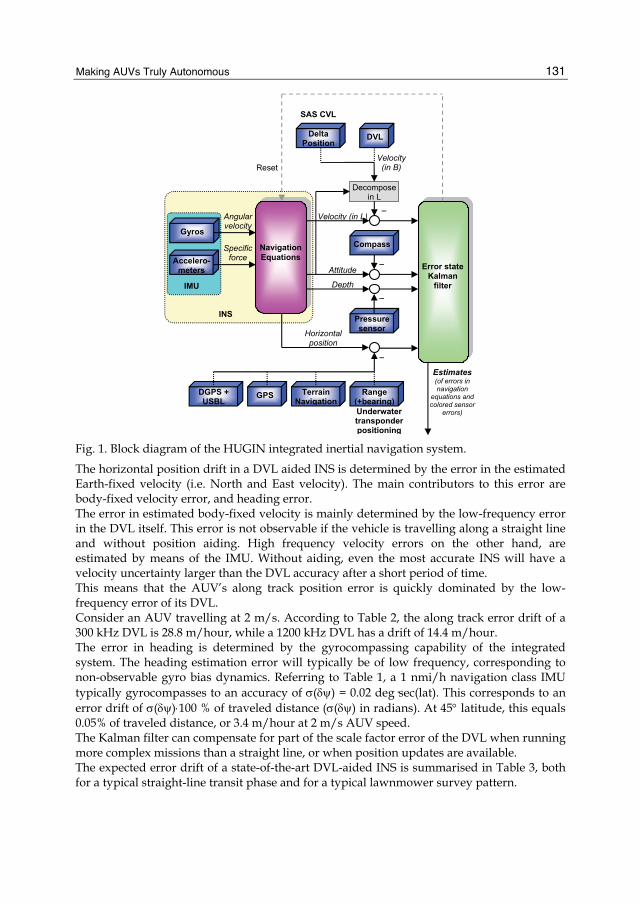
2.1 Integrated inertial navigation system structure An INS calculates position, velocity and attitude using high frequency data from an Inertial Measurement Unit (IMU). An IMU consists of three accelerometers measuring specific force and three gyros measuring angular rate. If left unaided the INS will, after a short period of time, have unacceptable position errors. The position error growth is determined by the class of the IMU, see Table 1. Currently the best available IMU with a feasible size for an AUV gives a position error growth in the order of 1 nmi/h (1 σ), when integrated in an INS. To reduce this error the INS needs to be aided by redundant sensor measurements. These sensors are usually integrated with the INS through a Kalman filter, which performs this integration in a mathematically optimal manner. Fig 1 shows a schematic view of the HUGIN integrated INS, where the Kalman filter is based on an error-state model and provides a much higher total navigation performance than is obtained from the individual sensors alone.

IMU class Gyro bias Accelerometer bias >10 nmi/h 1°/h 1 mg

1 nmi/h 0.005°/h 30 μg

Table 1. Classification of feasible IMUs for AUVs

2.2 DVL aided INS The solution for most modern AUVs is a low drift Doppler Velocity Log (DVL) aided INS that can integrate various forms of position measurement updates. DVL accuracy is dependent on acoustic frequency. Higher frequency yields better accuracy at the cost of decreased range, as illustrated in Table 2. Prioritisation between range and accuracy is dependent on the application.

Frequency Long term accuracy Range 150 kHz ±0.5% o.s. ± 2 mm/s 425 – 500 m 300 kHz ±0.4% o.s. ± 2 mm/s 200 m 600 kHz ±0.2% o.s. ± 1 mm/s 90 m

1200 kHz ±0.2% o.s. ± 1 mm/s 30 m

Table 2. DVL range and accuracy depends on its acoustic frequency (o.s is of speed).

Making AUVs Truly Autonomous

131

DVLDelta Position

Navigation Equations

Gyros

Accelero-meters

Error state Kalman

filter

Velocity (in B)

Decompose in L

Velocity (in L)Angular velocity

Specific force

INS

IMU

Compass

Pressure sensor

_

_

_

Attitude

Depth

_

Range (+bearing)

Terrain Navigation

GPS DGPS + USBL

Estimates (of errors in navigation

equations and colored sensor

errors)

SAS CVL

Underwater transponder positioning

Reset

Horizontal position

Fig. 1. Block diagram of the HUGIN integrated inertial navigation system.

The horizontal position drift in a DVL aided INS is determined by the error in the estimated Earth-fixed velocity (i.e. North and East velocity). The main contributors to this error are body-fixed velocity error, and heading error. The error in estimated body-fixed velocity is mainly determined by the low-frequency error in the DVL itself. This error is not observable if the vehicle is travelling along a straight line and without position aiding. High frequency velocity errors on the other hand, are estimated by means of the IMU. Without aiding, even the most accurate INS will have a velocity uncertainty larger than the DVL accuracy after a short period of time. This means that the AUV’s along track position error is quickly dominated by the low-frequency error of its DVL. Consider an AUV travelling at 2 m/s. According to Table 2, the along track error drift of a 300 kHz DVL is 28.8 m/hour, while a 1200 kHz DVL has a drift of 14.4 m/hour. The error in heading is determined by the gyrocompassing capability of the integrated system. The heading estimation error will typically be of low frequency, corresponding to non-observable gyro bias dynamics. Referring to Table 1, a 1 nmi/h navigation class IMU typically gyrocompasses to an accuracy of σ(δψ) = 0.02 deg·sec(lat). This corresponds to an error drift of σ(δψ)⋅100 % of traveled distance (σ(δψ) in radians). At 45° latitude, this equals 0.05% of traveled distance, or 3.4 m/hour at 2 m/s AUV speed. The Kalman filter can compensate for part of the scale factor error of the DVL when running more complex missions than a straight line, or when position updates are available. The expected error drift of a state-of-the-art DVL-aided INS is summarised in Table 3, both for a typical straight-line transit phase and for a typical lawnmower survey pattern.

Underwater Vehicles

132

Position error drift (% of traveled distance)

Straight line

Lawnmower pattern with 1 km

lines Along track 0.11% 0.01% Across track 0.03% 0.001%

Table 3. Typical position error drift for a high quality DVL-aided INS

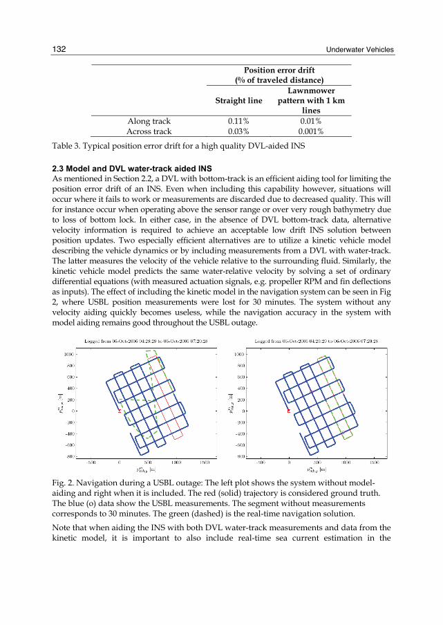
2.3 Model and DVL water-track aided INS As mentioned in Section 2.2, a DVL with bottom-track is an efficient aiding tool for limiting the position error drift of an INS. Even when including this capability however, situations will occur where it fails to work or measurements are discarded due to decreased quality. This will for instance occur when operating above the sensor range or over very rough bathymetry due to loss of bottom lock. In either case, in the absence of DVL bottom-track data, alternative velocity information is required to achieve an acceptable low drift INS solution between position updates. Two especially efficient alternatives are to utilize a kinetic vehicle model describing the vehicle dynamics or by including measurements from a DVL with water-track. The latter measures the velocity of the vehicle relative to the surrounding fluid. Similarly, the kinetic vehicle model predicts the same water-relative velocity by solving a set of ordinary differential equations (with measured actuation signals, e.g. propeller RPM and fin deflections as inputs). The effect of including the kinetic model in the navigation system can be seen in Fig 2, where USBL position measurements were lost for 30 minutes. The system without any velocity aiding quickly becomes useless, while the navigation accuracy in the system with model aiding remains good throughout the USBL outage.

Fig. 2. Navigation during a USBL outage: The left plot shows the system without model-aiding and right when it is included. The red (solid) trajectory is considered ground truth. The blue (o) data show the USBL measurements. The segment without measurements corresponds to 30 minutes. The green (dashed) is the real-time navigation solution.

Note that when aiding the INS with both DVL water-track measurements and data from the kinetic model, it is important to also include real-time sea current estimation in the

Making AUVs Truly Autonomous

133

navigation system. The sea current will often constitute the dominant error source when aiding the INS with water-relative velocity data, in particular when applying DVL water track data. For additional information on model-aiding and sea current estimation, the reader may refer to (Hegrenæs et al., 2007) and (Hegrenæs et al., 2008).

2.4 Micro delta-position aiding Some of the sensors carried by an AUV can observe the same part of the seafloor in consecutive sensor measurements, such as a Synthetic Aperture Sonar (SAS), a 3D sonar, or a camera. By correlating these consecutive measurements of the same seafloor patch over a small time interval, a measurement of the change of the AUVs position between these measurement times may be derived. A Correlation Velocity Log (CVL) is another sensor that provides a similar measurement, although using a different measurement principle. These sensors provide a different measurement than velocity to integrate with the INS. This aiding technique is herein called micro delta-position aiding. When the time interval is very short, the measurement more and more resembles a pure velocity measurement. This technique therefore provides redundancy to the DVL, but may also decrease the position error drift of the DVL-aided INS substantially if the measurement is sufficiently accurate. In this aspect, SAS is a particularly attractive sensor. SAS uses consecutive pings to synthesise a larger array. For this to work properly, the array position displacement between pings must be found with extremely high accuracy. This is called micronavigation or DPCA (displaced phase centre antenna) (Belletini & Pinto, 2002; Hansen et. al., 2003). By using this position displacement as a velocity measurement, it can potentially be an order of magnitude better than even the most accurate DVL. The technique is fully autonomous, but requires a suitable sensor onboard the AUV.

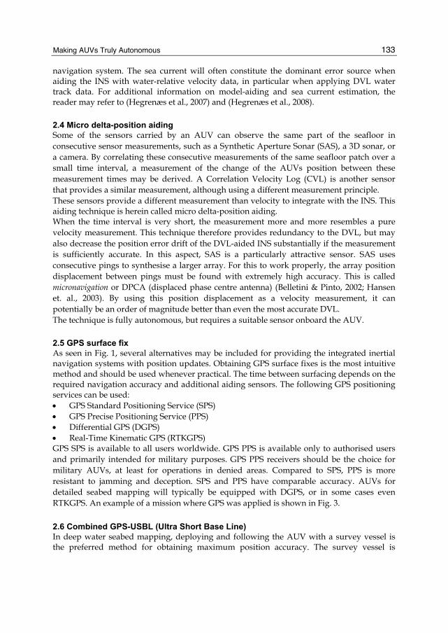
2.5 GPS surface fix As seen in Fig. 1, several alternatives may be included for providing the integrated inertial navigation systems with position updates. Obtaining GPS surface fixes is the most intuitive method and should be used whenever practical. The time between surfacing depends on the required navigation accuracy and additional aiding sensors. The following GPS positioning services can be used: • GPS Standard Positioning Service (SPS) • GPS Precise Positioning Service (PPS) • Differential GPS (DGPS) • Real-Time Kinematic GPS (RTKGPS) GPS SPS is available to all users worldwide. GPS PPS is available only to authorised users and primarily intended for military purposes. GPS PPS receivers should be the choice for military AUVs, at least for operations in denied areas. Compared to SPS, PPS is more resistant to jamming and deception. SPS and PPS have comparable accuracy. AUVs for detailed seabed mapping will typically be equipped with DGPS, or in some cases even RTKGPS. An example of a mission where GPS was applied is shown in Fig. 3.

2.6 Combined GPS-USBL (Ultra Short Base Line) In deep water seabed mapping, deploying and following the AUV with a survey vessel is the preferred method for obtaining maximum position accuracy. The survey vessel is

Underwater Vehicles

134

-1 -0.5 0 0.5 1

x 104

0

0.2

0.4

0.6

0.8

1

1.2

1.4

1.6

1.8

2x 104 Position relative to start of navigation (0,0).

East (m)

Nor

th (m

)

HUGIN INS positionStart pointGPS surface fix

Start of mission

End of mission

Fig. 3. Mission example with GPS surface fix using a HUGIN AUV, September 2003.

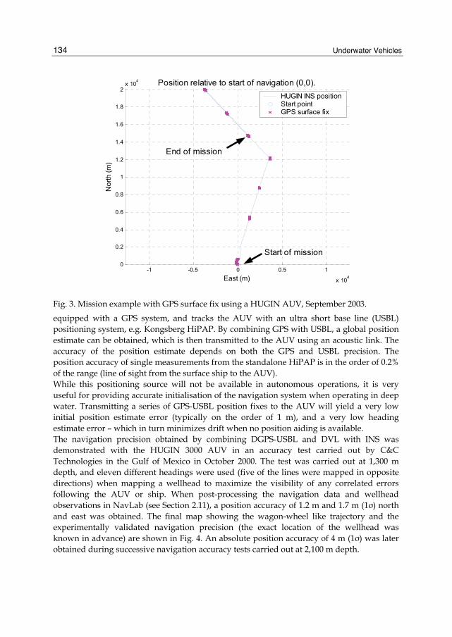
equipped with a GPS system, and tracks the AUV with an ultra short base line (USBL) positioning system, e.g. Kongsberg HiPAP. By combining GPS with USBL, a global position estimate can be obtained, which is then transmitted to the AUV using an acoustic link. The accuracy of the position estimate depends on both the GPS and USBL precision. The position accuracy of single measurements from the standalone HiPAP is in the order of 0.2% of the range (line of sight from the surface ship to the AUV). While this positioning source will not be available in autonomous operations, it is very useful for providing accurate initialisation of the navigation system when operating in deep water. Transmitting a series of GPS-USBL position fixes to the AUV will yield a very low initial position estimate error (typically on the order of 1 m), and a very low heading estimate error – which in turn minimizes drift when no position aiding is available. The navigation precision obtained by combining DGPS-USBL and DVL with INS was demonstrated with the HUGIN 3000 AUV in an accuracy test carried out by C&C Technologies in the Gulf of Mexico in October 2000. The test was carried out at 1,300 m depth, and eleven different headings were used (five of the lines were mapped in opposite directions) when mapping a wellhead to maximize the visibility of any correlated errors following the AUV or ship. When post-processing the navigation data and wellhead observations in NavLab (see Section 2.11), a position accuracy of 1.2 m and 1.7 m (1σ) north and east was obtained. The final map showing the wagon-wheel like trajectory and the experimentally validated navigation precision (the exact location of the wellhead was known in advance) are shown in Fig. 4. An absolute position accuracy of 4 m (1σ) was later obtained during successive navigation accuracy tests carried out at 2,100 m depth.

Making AUVs Truly Autonomous

135

Fig. 4. A wellhead mapped repeatedly with different headings to evaluate the position accuracy of the final map, and hence the navigation system. The true position of the wellhead was located at coordinates (0,0) relative north and east.

2.7 LBL (Long Base Line) Underwater transponders may be used to provide submerged position measurements to the AUV. If multiple transponders are arranged in a network for this purpose, it is called a long base line (LBL) system. The AUV interrogates the LBL network, and uses the reply from each transponder to calculate the range from the AUV to the transponders. If the 3D position of each transponder is known, the AUV can compute a unique position by triangulation if replies are received from three or more transponders. If only two transponders are within range (sparse LBL system), two possible position solutions exist. These are mirrored about the base line between the transponders. The LBL network is deployed and calibrated by a surface vessel, and is therefore not a strictly autonomous solution. However, once the network is established, the AUV may navigate autonomously with bounded error drift by visiting the network occasionally.

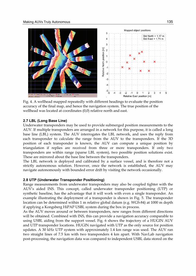
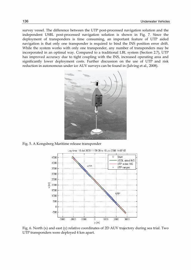
2.8 UTP (Underwater Transponder Positioning) Range measurements from underwater transponders may also be coupled tighter with the AUV’s aided INS. This concept, called underwater transponder positioning (UTP) or synthetic baseline, has the advantage that it will work with even a single transponder. An example illustrating the deployment of a transponder is shown in Fig. 5. The transponder location can be determined within 1 m relative global datum (e.g. WGS-84) at 1000 m depth if applying a Kongsberg HiPAP USBL system during the box in process. As the AUV moves around or between transponders, new ranges from different directions will be obtained. Combined with INS, this can provide a navigation accuracy comparable to using USBL aiding from the support vessel. Fig. 6 shows the trajectory of a HUGIN AUV and UTP transponder locations. HUGIN navigated with UTP as the only source for position updates. A 30 kHz UTP system with approximately 1.4 km range was used. The AUV ran two straight lines of 7.5 km with two transponders 4 km apart. With NavLab navigation post-processing, the navigation data was compared to independent USBL data stored on the

Underwater Vehicles

136

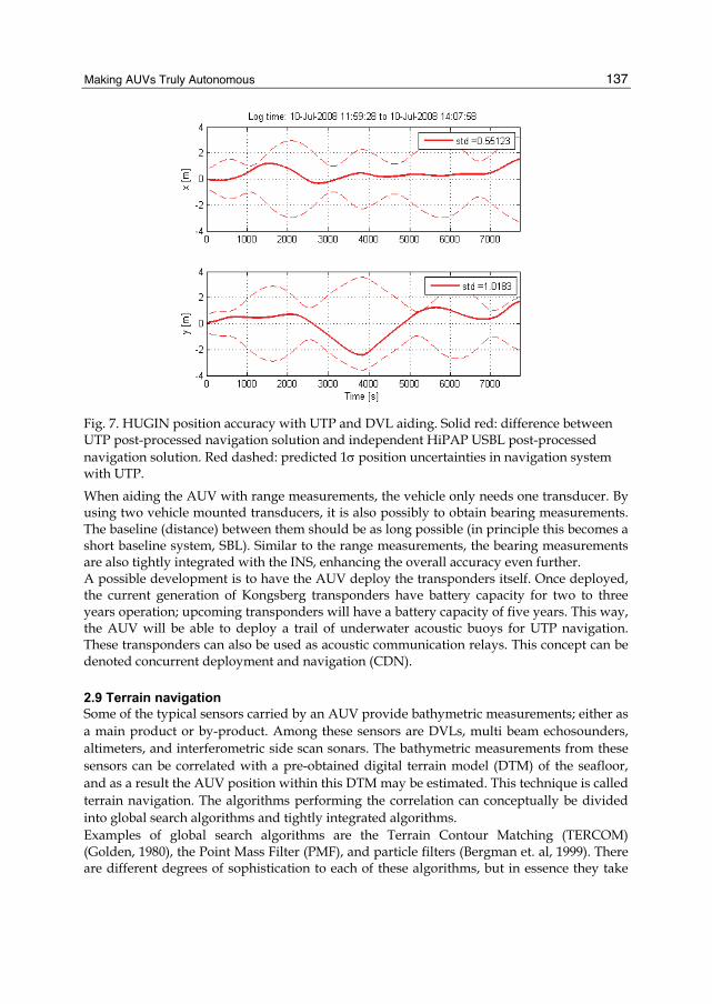
survey vessel. The difference between the UTP post-processed navigation solution and the independent USBL post-processed navigation solution is shown in Fig. 7. Since the deployment of transponders is time consuming, an important feature of UTP aided navigation is that only one transponder is required to bind the INS position error drift. While the system works with only one transponder, any number of transponders may be incorporated in an optimal way. Compared to a traditional LBL system (Section 2.7), UTP has improved accuracy due to tight coupling with the INS, increased operating area and significantly lower deployment costs. Further discussion on the use of UTP and risk reduction in autonomous under ice AUV surveys can be found in (Jalving et al., 2008).

Fig. 5. A Kongsberg Maritime release transponder

Fig. 6. North (x) and east (y) relative coordinates of 2D AUV trajectory during sea trial. Two UTP transponders were deployed 4 km apart.

Making AUVs Truly Autonomous

137

Fig. 7. HUGIN position accuracy with UTP and DVL aiding. Solid red: difference between UTP post-processed navigation solution and independent HiPAP USBL post-processed navigation solution. Red dashed: predicted 1σ position uncertainties in navigation system with UTP.

When aiding the AUV with range measurements, the vehicle only needs one transducer. By using two vehicle mounted transducers, it is also possibly to obtain bearing measurements. The baseline (distance) between them should be as long possible (in principle this becomes a short baseline system, SBL). Similar to the range measurements, the bearing measurements are also tightly integrated with the INS, enhancing the overall accuracy even further. A possible development is to have the AUV deploy the transponders itself. Once deployed, the current generation of Kongsberg transponders have battery capacity for two to three years operation; upcoming transponders will have a battery capacity of five years. This way, the AUV will be able to deploy a trail of underwater acoustic buoys for UTP navigation. These transponders can also be used as acoustic communication relays. This concept can be denoted concurrent deployment and navigation (CDN).

2.9 Terrain navigation Some of the typical sensors carried by an AUV provide bathymetric measurements; either as a main product or by-product. Among these sensors are DVLs, multi beam echosounders, altimeters, and interferometric side scan sonars. The bathymetric measurements from these sensors can be correlated with a pre-obtained digital terrain model (DTM) of the seafloor, and as a result the AUV position within this DTM may be estimated. This technique is called terrain navigation. The algorithms performing the correlation can conceptually be divided into global search algorithms and tightly integrated algorithms. Examples of global search algorithms are the Terrain Contour Matching (TERCOM) (Golden, 1980), the Point Mass Filter (PMF), and particle filters (Bergman et. al, 1999). There are different degrees of sophistication to each of these algorithms, but in essence they take

Underwater Vehicles

138

input from the INS, a bathymetric sensor and a DTM, and estimate a global position measurement to be integrated back with the INS. These algorithms handle highly non-linear bathymetry with great results, but have convergence problems in terrain with little variation. The tightly integrated algorithms, such as Terrain Referenced Integrated Navigation (TRIN) (Hagen & Hagen, 2000), and Sandia Integrated Terrain Aided Navigation (SITAN) (Hostetler, 1978), integrate the bathymetric range measurements tightly with the INS. These algorithms handle linear and weakly non-linear terrain very well, but may have some problems with highly non-linear terrain. Terrain navigation is a fully autonomous technique, but it requires a DTM of the mission area. This information is unfortunately not always available. A solution to this problem is called Concurrent Mapping and Navigation (CMN), where the DTM is made by the AUV in-situ, and used concurrently by the terrain navigation algorithms to bind the position error drift.

-20 -10 0 10 20 30 40 50 60 70

-20

0

20

40

60

80

100

East offset[m]

Nor

th o

ffset

[m]

Point Mass PDF Contours after 9 pings

-40 -20 0 20 40 60-40

-20

0

20

40

60

80

100

120

East offset[m]

Nor

th o

ffset

[m]

Particle Filter cloud after 9 pings

Fig. 8. The contour lines of the PMF’s probability density function (left) and the particle filter cloud (right) after processing 9 pings from a DVL with the tool TerrLab (Hagen, 2006). Red line is a priori navigation solution, black line is true position and cyan marks position estimates from the terrain navigation algorithms.

2.10 Macro delta-position aiding As an extension of the idea of the micro delta-position aiding, we can consider sensor measurements where the same patch of the seafloor is seen with an arbitrarily large time interval between the measurements. As an example, consider the detection of mine-like objects from sidescan images. If the AUV passes the same object multiple times, and the localisation accuracy of the object is mainly contributed to the AUVs navigation accuracy, then the difference between the object’s estimated position from the two observation times gives a valuable measurement of relative position error of the AUV. This type of measurement can be integrated with an INS, and the technique is herein called macro delta-position aiding. Another example, closely related to CMN, is to use sparse bathymetric information from an interferometric sonar covering overlapping regions during the mission. After running one of the terrain navigation algorithms, we will be able to make a macro delta-position measurement for the INS.

Making AUVs Truly Autonomous

139

This technique is fully autonomous, but requires an imaging or bathymetric sensor. It is also only possible to bind the position error drift with this technique. The initial global error of the AUV is not observed, as can be done with regular terrain navigation

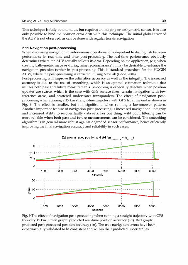
2.11 Navigation post-processing When discussing navigation in autonomous operations, it is important to distinguish between performance in real time and after post-processing. The real-time performance obviously determines where the AUV actually collects its data. Depending on the application, (e.g. when creating bathymetric maps or during mine reconnaissance) it may be desirable to enhance the navigation precision further in post-processing. This is standard procedure for the HUGIN AUVs, where the post-processing is carried out using NavLab (Gade, 2004). Post-processing will improve the estimation accuracy as well as the integrity. The increased accuracy is due to the use of smoothing, which is an optimal estimation technique that utilizes both past and future measurements. Smoothing is especially effective when position updates are scarce, which is the case with GPS surface fixes, terrain navigation with few reference areas, and scattered underwater transponders. The effect of navigation post-processing when running a 15 km straight-line trajectory with GPS fix at the end is shown in Fig. 9. The effect is smaller, but still significant, when running a lawnmower pattern. Another important feature of navigation post-processing is increased navigational integrity and increased ability to recover faulty data sets. For one thing, wild point filtering can be more reliable when both past and future measurements can be considered. The smoothing algorithm is in general more robust against degraded sensor performance, hence efficiently improving the final navigation accuracy and reliability in such cases.

Fig. 9.The effect of navigation post-processing when running a straight trajectory with GPS fix every 15 km. Green graph: predicted real-time position accuracy (1σ). Red graph: predicted post-processed position accuracy (1σ). The true navigation errors have been experimentally validated to be consistent and within their predicted uncertainties.

Underwater Vehicles

140

3. Decision autonomy The vast majority of today’s AUVs operate with a pre-programmed mission plan specifying waypoints and vehicle parameters for the entire mission. Complex tasks that cannot be accurately specified in advance must be solved through intermittent communication with a human operator. This obviously limits the performance and applicability of such vehicles. A truly autonomous vehicle must be able to perceive its own condition and its environment, and respond appropriately to unexpected or dynamic situations. Updated situational awareness requires an extensive set of sensors and data analysis tools, but the most challenging part of decision autonomy is still to select advantageous actions based on the information available. Conceptually, decision autonomy can be divided into two categories: The ability to handle internal malfunctions (sustainability) – and the ability to handle unpredictable external events (adaptivity). The latter is important for optimizing mission execution by adaptive, real-time mission planning based on e.g. observed bathymetry and sea current conditions. It also facilitates novel applications such as adaptive data collection and cooperation with other vehicles. Sustainability is vital to realise both long-endurance missions, as the probability of sub-system failures increases with mission duration, and missions in extreme environments, e.g. under ice, where consequences of failures may be unacceptable. In all cases, actions must be chosen so that the overall mission goals are achieved to highest degree possible. These actions may include modifying the mission plan, and algorithms for automated re-planning are thus required. Section 3.1 provides an overview of the different architectures that are common to use when designing an autonomous control system. Section 3.2 introduces autonomous path planning, explaining the consequences of the control architecture on the complexity of the planning algorithms. Planning requires knowledge about the environment of the vehicle, and Section 3.3 discusses ways to represent this knowledge. For the vehicle to be truly autonomous, it is important that its sensors are also able to operate autonomously; this is discussed in Section 3.4. The ability to handle internal malfunctions is covered in Section 3.5. The autonomous vehicle may be required to cooperate with other vehicles, both autonomous and not. Some scenarios requiring such cooperation are given in Section 3.6. Finally, an example of an autonomous vehicle is given in Section 3.7, which very briefly describes the autonomy system of the HUGIN AUV.

3.1 Control architectures A control architecture is a software framework that manages both sensor and actuator systems, thus enabling the AUV to perform a user-specified mission. There are basically three different approaches to control architectures: deliberate, reactive and hybrid systems (Arkin, 1998)(Valavanis et al, 1998)(Ridao et al., 2000)(Russell & Norvig, 2003). Deliberate (hierarchical) architectures are based on planning using a world model. They allow reasoning and making predictions about the environment. Data flows from sensors to the world model, which is used together with a predefined set of mission goals to plan new actions to be undertaken by the actuators (Fig 10). This “Sense-Plan-Act” scheme is suited for structured and predictable environments, and its well-defined, tightly-coupled structure simplifies the process of system design and verification. However, problems arise when trying to maintain an accurate, real-time world model in the complex, dynamic and only partly observable environments typical for underwater operation. System response may then be too slow or erratic.

Making AUVs Truly Autonomous

141

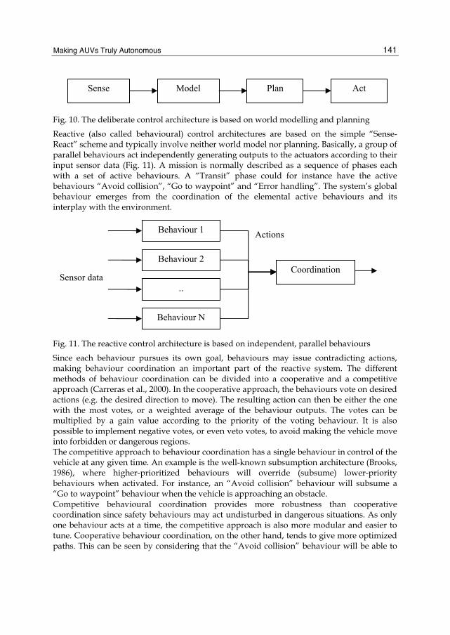
Fig. 10. The deliberate control architecture is based on world modelling and planning

Reactive (also called behavioural) control architectures are based on the simple “Sense-React” scheme and typically involve neither world model nor planning. Basically, a group of parallel behaviours act independently generating outputs to the actuators according to their input sensor data (Fig. 11). A mission is normally described as a sequence of phases each with a set of active behaviours. A “Transit” phase could for instance have the active behaviours “Avoid collision”, “Go to waypoint” and “Error handling”. The system’s global behaviour emerges from the coordination of the elemental active behaviours and its interplay with the environment.

Fig. 11. The reactive control architecture is based on independent, parallel behaviours

Since each behaviour pursues its own goal, behaviours may issue contradicting actions, making behaviour coordination an important part of the reactive system. The different methods of behaviour coordination can be divided into a cooperative and a competitive approach (Carreras et al., 2000). In the cooperative approach, the behaviours vote on desired actions (e.g. the desired direction to move). The resulting action can then be either the one with the most votes, or a weighted average of the behaviour outputs. The votes can be multiplied by a gain value according to the priority of the voting behaviour. It is also possible to implement negative votes, or even veto votes, to avoid making the vehicle move into forbidden or dangerous regions. The competitive approach to behaviour coordination has a single behaviour in control of the vehicle at any given time. An example is the well-known subsumption architecture (Brooks, 1986), where higher-prioritized behaviours will override (subsume) lower-priority behaviours when activated. For instance, an “Avoid collision” behaviour will subsume a “Go to waypoint” behaviour when the vehicle is approaching an obstacle. Competitive behavioural coordination provides more robustness than cooperative coordination since safety behaviours may act undisturbed in dangerous situations. As only one behaviour acts at a time, the competitive approach is also more modular and easier to tune. Cooperative behaviour coordination, on the other hand, tends to give more optimized paths. This can be seen by considering that the “Avoid collision” behaviour will be able to

Actions Behaviour 1

Behaviour 2

..

Behaviour N

Sensor data Coordination

Sense Model Plan Act

Underwater Vehicles

142

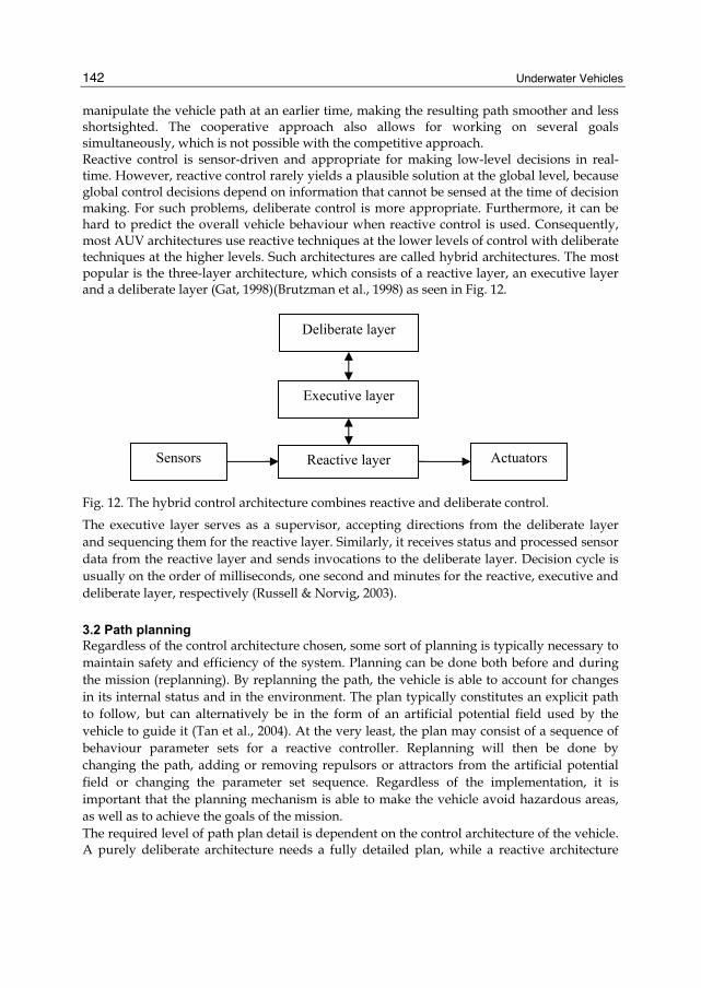
manipulate the vehicle path at an earlier time, making the resulting path smoother and less shortsighted. The cooperative approach also allows for working on several goals simultaneously, which is not possible with the competitive approach. Reactive control is sensor-driven and appropriate for making low-level decisions in real-time. However, reactive control rarely yields a plausible solution at the global level, because global control decisions depend on information that cannot be sensed at the time of decision making. For such problems, deliberate control is more appropriate. Furthermore, it can be hard to predict the overall vehicle behaviour when reactive control is used. Consequently, most AUV architectures use reactive techniques at the lower levels of control with deliberate techniques at the higher levels. Such architectures are called hybrid architectures. The most popular is the three-layer architecture, which consists of a reactive layer, an executive layer and a deliberate layer (Gat, 1998)(Brutzman et al., 1998) as seen in Fig. 12.

Fig. 12. The hybrid control architecture combines reactive and deliberate control.

The executive layer serves as a supervisor, accepting directions from the deliberate layer and sequencing them for the reactive layer. Similarly, it receives status and processed sensor data from the reactive layer and sends invocations to the deliberate layer. Decision cycle is usually on the order of milliseconds, one second and minutes for the reactive, executive and deliberate layer, respectively (Russell & Norvig, 2003).

3.2 Path planning Regardless of the control architecture chosen, some sort of planning is typically necessary to maintain safety and efficiency of the system. Planning can be done both before and during the mission (replanning). By replanning the path, the vehicle is able to account for changes in its internal status and in the environment. The plan typically constitutes an explicit path to follow, but can alternatively be in the form of an artificial potential field used by the vehicle to guide it (Tan et al., 2004). At the very least, the plan may consist of a sequence of behaviour parameter sets for a reactive controller. Replanning will then be done by changing the path, adding or removing repulsors or attractors from the artificial potential field or changing the parameter set sequence. Regardless of the implementation, it is important that the planning mechanism is able to make the vehicle avoid hazardous areas, as well as to achieve the goals of the mission. The required level of path plan detail is dependent on the control architecture of the vehicle. A purely deliberate architecture needs a fully detailed plan, while a reactive architecture

Deliberate layer

Executive layer

Reactive layer Sensors Actuators

Making AUVs Truly Autonomous

143

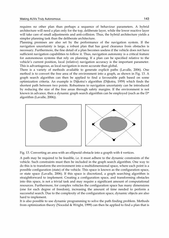
requires no other plan than perhaps a sequence of behaviour parameters. A hybrid architecture will need a plan only for the top, deliberate layer, while the lower reactive layer will take care of small adjustments and anti-collision. Thus, the hybrid architecture yields a simpler planning task than the deliberate architecture. Planning premises are also set by the performance of the navigation system. If the navigation uncertainty is large, a robust plan that has good clearance from obstacles is necessary. Furthermore, the fine detail of a plan becomes useless if the vehicle does not have sufficient navigation capabilities to follow it. Thus, navigation autonomy is a critical feature for autonomous systems that rely on planning. If a plan can be specified relative to the vehicle’s current position, local (relative) navigation accuracy is the important parameter. This is advantageous, as local navigation is more accurate than global. There is a variety of methods available to generate explicit paths (Lavalle, 2006). One method is to convert the free area of the environment into a graph, as shown in Fig. 13. A graph search algorithm can then be applied to find a favourable path based on some optimization criteria. An example is Dijkstra’s algorithm (Dijkstra, 1959) which finds the shortest path between two points. Robustness to navigation uncertainty can be introduced by reducing the size of the free areas through safety margins. If the environment is not known in advance, then a dynamic graph search algorithm can be employed (such as the D* algorithm (Lavalle, 2006)).

Fig. 13. Converting an area with an ellipsoid obstacle into a grapth with 4 vertices.

A path may be required to be feasible, i.e. it must adhere to the dynamic constraints of the vehicle. Such constraints must then be included in the graph search algorithm. One way to do this is to transform the environment into a multidimensional space, where each point is a possible configuration (state) of the vehicle. This space is known as the configuration space, or state space (Lavalle, 2006). If this space is discretized, a graph searching algorithm is straightforward to implement. Creating a configuration space, and transforming obstacles into this space, is not a trivial task and may require a significant amount of computational resources. Furthermore, for complex vehicles the configuration space has many dimensions (one for each degree of freedom), increasing the amount of time needed to perform a successful search. Due to the complexity of the configuration space, dynamic objects are also hard to implement. It is also possible to use dynamic programming to solve the path finding problem. Methods from optimization theory (Nocedal & Wright, 1999) can then be applied to find a plan that is

Underwater Vehicles

144

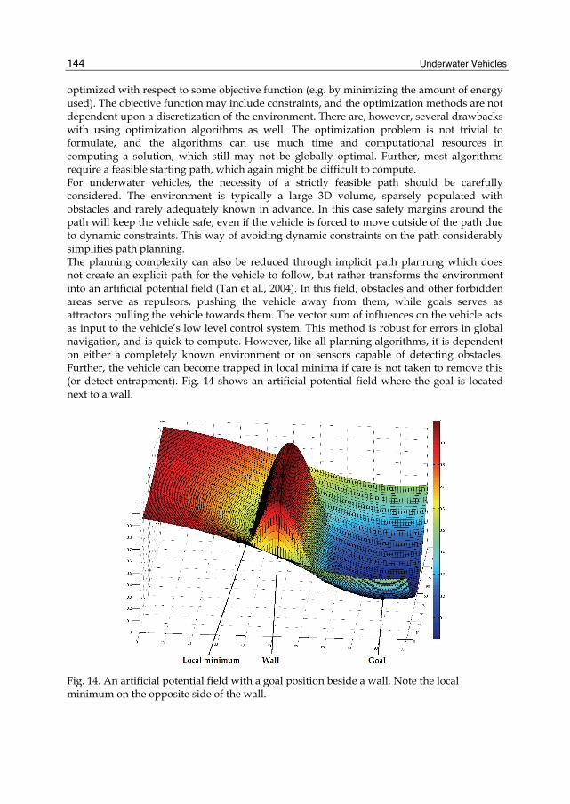
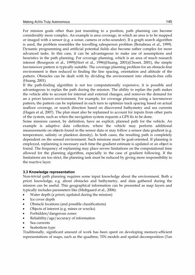
optimized with respect to some objective function (e.g. by minimizing the amount of energy used). The objective function may include constraints, and the optimization methods are not dependent upon a discretization of the environment. There are, however, several drawbacks with using optimization algorithms as well. The optimization problem is not trivial to formulate, and the algorithms can use much time and computational resources in computing a solution, which still may not be globally optimal. Further, most algorithms require a feasible starting path, which again might be difficult to compute. For underwater vehicles, the necessity of a strictly feasible path should be carefully considered. The environment is typically a large 3D volume, sparsely populated with obstacles and rarely adequately known in advance. In this case safety margins around the path will keep the vehicle safe, even if the vehicle is forced to move outside of the path due to dynamic constraints. This way of avoiding dynamic constraints on the path considerably simplifies path planning. The planning complexity can also be reduced through implicit path planning which does not create an explicit path for the vehicle to follow, but rather transforms the environment into an artificial potential field (Tan et al., 2004). In this field, obstacles and other forbidden areas serve as repulsors, pushing the vehicle away from them, while goals serves as attractors pulling the vehicle towards them. The vector sum of influences on the vehicle acts as input to the vehicle’s low level control system. This method is robust for errors in global navigation, and is quick to compute. However, like all planning algorithms, it is dependent on either a completely known environment or on sensors capable of detecting obstacles. Further, the vehicle can become trapped in local minima if care is not taken to remove this (or detect entrapment). Fig. 14 shows an artificial potential field where the goal is located next to a wall.

Fig. 14. An artificial potential field with a goal position beside a wall. Note the local minimum on the opposite side of the wall.

Making AUVs Truly Autonomous

145

For mission goals other than just transiting to a position, path planning can become considerably more complex. An example is area coverage, in which an area is to be mapped or imaged with a sensor (e.g. a sonar, camera or echo-sounder). If a graph search algorithm is used, the problem resembles the travelling salesperson problem (Bonabeau et al., 1999). Dynamic programming and artificial potential fields also become rather complex for more advanced tasks. In this case, it can be advantageous to make use of assumptions and heuristics in the path planning. For coverage planning, which is an area of much research interest (Bourgeois et al., 1999)(Hert et al., 1996)(Huang, 2001)(Choset, 2001), the simple lawnmower pattern is typically suitable. The coverage planning problem for an obstacle-free environment is then reduced to finding the line spacing, orientation and altitude of the pattern. Obstacles can be dealt with by dividing the environment into obstacle-free cells (Huang, 2001). If the path-finding algorithm is not too computationally expensive, it is possible and advantageous to replan the path during the mission. The ability to replan the path makes the vehicle able to account for internal and external changes, and removes the demand for an a priori known environment. For example, for coverage planning using a lawnmower pattern, the pattern can be replanned in each turn to optimize track spacing based on actual seafloor coverage, or search direction based on discovered bathymetry and sea currents (Hagen et al, 2007). The plan must also be replanned to account for inputs from other parts of the system, such as when the navigation system requests a GPS fix to be done. Some missions cannot, by definition, have an explicit, planned path for the vehicle. An example is adaptive data collection, where the vehicle may perform additional measurements on objects found in the sensor data or may follow a sensor data gradient (e.g. temperature, salinity or plankton density). In both cases, the resulting path is completely dependent on the sensed environment. Such missions must be goal-oriented. If planning is employed, replanning is necessary each time the gradient estimate is updated or an object is found. The frequency of replanning may place severe limitations on the computational time allowed for the planning algorithm, especially in the case of gradient following. If the limitations are too strict, the planning task must be reduced by giving more responsibility to the reactive layer.

3.3 Knowledge representation Non-trivial path planning requires some input knowledge about the environment. Both a priori knowledge, e.g. about obstacles and bathymetry, and data gathered during the mission can be useful. This geographical information can be presented as map layers and typically includes parameters like (Midtgaard et al., 2006): • Water depth (a priori; updated during the mission) • Ice cover depth • Obstacle locations (and possible classifications) • Objects of interest (e.g. mines or wrecks) • Forbidden/dangerous zones • Reliability/age/accuracy of information • Sea currents • Seabottom type Traditionally, significant amount of work has been spent on developing memory-efficient representations of maps, such as the quadtree, TIN models and spatial decomposition (Tan

Underwater Vehicles

146

et al., 2004). While these methods may reduce memory requirements by several orders of magnitude without loss of information, the time to access information can increase dramatically. Current start-of-the-art computer systems have enough memory storage to make a uniform grid representation a reasonable choice. For a deliberate architecture, dependent on a high level of planning, the required grid spacing of the map is set in a large part by the environment. If the environment is simple with a sparse obstacle density, only a coarse map is required. However, a complex environment (e.g. a harbour) requires a fine-gridded map. A reactive architecture may not need a map at all, or only a very coarse one, regardless of the environment. A hybrid architecture, with a top deliberate layer and a bottom reactive layer, only needs a plan for the deliberate layer. Thus, it only requires a coarse gridding on the map in any environment. How coarse is dependent both on the mission an on how much of the control is performed by the deliberate and how much is performed by the reactive layer. Note that the product of the mission, e.g. a bathymetric map, will typically be stored in another, high-resolution format that need not be kept in memory.

3.4 Sensor autonomy To the end user, an AUV is nothing more than a platform carrying the sensors (or other payloads) that perform the actual objective of the mission; data collection. In fully autonomous HUGIN missions, the performance of the onboard sensors and other subsystems are normally checked during the initial phase of the mission, where the AUV is within communication range of the surface vessel. Using either acoustic or RF links, the operator can ensure that all subsystems perform as assumed during the planning phase – and take corrective action as needed. If conditions are known to vary, different sensor settings may be pre-programmed for different parts of the mission plan. However, when operating autonomously in areas where the environmental conditions are unknown or rapidly varying, this may not be sufficient and the AUV will need to re-adjust the sensor configuration autonomously. Some sensors include some functionality for automatic adaptation to varying conditions; some are very simple and have no parameters that can be changed. However, most sensors available today are designed based on the assumption that a human operator will monitor the sensor data and adjust the sensor parameters as needed. This is in particular true for more advanced sensors such as side scan sonars, multibeam echo sounders, synthetic aperture sonars and optical imaging systems. Over the following paragraphs, we will use the Kongsberg HISAS 1030 interferometric synthetic aperture sonar (SAS) as an example (Fossum et al., 2008). This sensor is used for very high resolution imaging (2-5 cm both along- and across-track) and high resolution bathymetry out to approximately 10 times AUV altitude. HISAS 1030 transmits wide-beam, wide-band pulses to port and starboard side at regular intervals; typically, a few Hz. Signals reflected back from the seafloor and from objects in the water volume are received in two long multi-element receiver arrays, as well as in the transmitter. A complex signal processing chain, working on data from a number of consecutive pings, transforms the raw data into sonar imagery and bathymetry (Hagen et al., 2001)(Hansen et al., 2003).

Making AUVs Truly Autonomous

147

The performance of a SAS is limited by a wide range of factors – AUV altitude, stability of motion, navigation accuracy, self noise, and sound speed variations, to name a few. In shallow water, performance is often limited by acoustic multipath; i.e., simultaneous reception of signals that have travelled different paths from transmitter to receiver (reflected from the seafloor, from the surface, seafloor then surface, surface then seafloor, etc). A fully autonomous SAS would analyse the returned signal and, based on the sonar data and knowledge of the environment, tune operation to optimize performance. The most obvious candidate parameters to modify include the transmission beam width and direction, and the AUV altitude. After applying these changes, the autonomy system may determine that performance is still inadequate; e.g., the actual range to which good sonar imagery can be produced is less than required to achieve full bottom coverage. This will then trigger replanning of the mission, by spacing survey lines tighter.

3.5 Error handling Robust error handling is vital to achieve sustainability and survivability of the vehicle. A conservative approach is to make the vehicle perform an emergency ascent when encountering any severe error or abnormal situation. This will ensure that the vehicle can be recovered, even though the result is mission failure. For under-ice or covert missions, an emergency ascent procedure will not be possible. Ensuring survival of the vehicle in emergency situations thus becomes significantly harder. In covert or clandestine operations, preventing discovery may be much more important than recovering the vehicle. In many scenarios, one option may be to perform an emergency descent, allowing the vehicle to rest at the sea floor until a recovery operation may be possible. Clearly, a more intelligent error handling will be needed for long endurance and complex missions. This will increase survival capabilities in dangerous situations as described above, and also enable the vehicle to complete the mission to the best degree possible. A challenge with error handling algorithms is that the error may be in the algorithm itself. This makes redundancy important, and necessitates a bottom-line error handling procedure with emergency ascent/descent. Intelligent error handling requires the vehicle to perceive both its external environment and internal status. By measuring sensor performance it is possible to alter the mission plan to optimize performance, as described under path planning. The vehicle should also be able to estimate the remaining time of operation before it runs out of energy, ensuring that it always has enough energy for the return journey. The error handling can be divided in three layers. The topmost layer is concerned with achieving the mission goals as best it can under the circumstances. This layer will be mission-dependent, and a different software module may be needed for each kind of mission. The middle layer is mission-independent and is concerned with getting the vehicle to the specified rendezvous position. The mission will not be a success, but the vehicle will at least be recovered at a safe location. The bottom layer is the last line of defence, and will attempt to ensure survivability of the vehicle. It is this layer that will perform emergency ascent/descent. The importance of the bottom layer makes it advantageous if this is implemented both in software and in hardware (e.g., if the power system suddenly fails, the hardware solution will ensure that an ascent procedure is initiated).

Underwater Vehicles

148

3.6 Cooperating systems Cooperating systems is a rising topic in the field of underwater intelligent vehicles providing many potential benefits. The systems can all be AUVs, or be a mixture of underwater and surface vehicles. Some vehicles may be autonomous while other may be remotely controlled or manned. Below are some examples of cooperation. The mission time to survey a given area may be significantly reduced by using several autonomous vehicles. The level of communication between these vehicles depends on the level of planning involved (and thus on the control architecture). If each vehicle is given a part of the area to explore independently, no intervehicle communication is necessary. However, it is also possible for the vehicles to interact, for instance by transmitting their positions and sensor findings as guidelines for the other vehicles. This is of particular interest for adaptive data collection, where the combined efforts of all the vehicles can be focused through either directions from a master AUV or control algorithms inspired by swarm intelligence (Bonabeau et al., 1999). The use of several AUVs moving in formation may be advantageous when tracking sensor data gradients, as calculating the spatial gradient based on data from a single vehicle requires intensive manoeuvring. Two AUVs with different sensor suites can cooperate in a mission where the objective is to detect and examine certain objects or features on the seafloor. The first vehicle is equipped with a sensor for long-range detection and covers the complete area using an efficient survey pattern (e.g. lawnmower). Sensor data is automatically processed in the vehicle, and results transmitted over acoustic link. The second vehicle is equipped with close-range inspection sensors and visits only the detection locations transmitted by the first vehicle. An AUV can cooperate with an accompanying surface ship in several ways. The surface ship (manned or unmanned) may provide an accurate position update to the AUV, using GPS and USBL as described in Section 2.6. The AUV can also acoustically transfer key parameters and data subsets to an unmanned surface vessel, which can use wireless communication to receivers located on land or in air, thus substantially increasing the effective communication range for the AUV. Another mode of cooperation is a bistatic sonar configuration. Typically the surface ship will transmit with an active sonar, with passive receiver antennas located on (or towed behind) one or more AUVs. The cooperation between an AUV and a manned military submarine also offers interesting possibilities. The AUV may be used as a forward sensor platform to avoid exposure of the submarine. As another example, the AUV may act as a decoy, using sonar to imitate a real submarine’s acoustic signature, thus deceiving the opponent. Planning of cooperative missions can primarily be divided in two areas. If the mission can be split into non-overlapping tasks each involving only a single vehicle, then these tasks can be planned separately. Each vehicle in the system will have one or more of these tasks, and will execute them independently of the others. The only procedure involving actual cooperation will be the distribution of tasks. However, if the mission can not be split into non-overlapping tasks, the planning will become very complex. Further, a high level of active cooperation between the vehicles will require a high level of communication. Long-range, high-bandwidth, networkable underwater communication is technically difficult to achieve, and also undesirable if the vehicles should avoid being detected. The level of

Making AUVs Truly Autonomous

149

cooperation is thus highly dependent on the mission, but it is evident that several missions can greatly benefit from using cooperating systems.

3.7 Implementation in the HUGIN AUV Goal driven mission management systems produce a mission plan based on the overall mission objectives together with relevant constraints and prior knowledge of the mission area. Such a system is being developed for the HUGIN AUV. A hybrid control architecture, as described in Section 3.1, is used. The deliberate layer has a hierarchical structure, dividing each task into smaller subtasks until the subtasks can be implemented by the lower, reactive layer. This gives much flexibility in placing the line between the deliberate and the reactive part, and the solution fits well into the existing HUGIN system. Using existing well-proven software as a starting point reduces the effort required for implementation and testing. It also facilitates a stepwise development approach, where new features can be tested at sea early in the process. While extensive testing can be performed in simulations, there is no substitute for testing AUV subsystems in their natural environment – the sea. This has been one of the main principles of the HUGIN development programme. A framework for autonomy has been designed and implemented, and is being integrated with the existing HUGIN control and mission management system. Among the first features to utilize this framework are an advanced anti-collision system, automated surfacing for GPS position updates (controlled by a variety of constraints), and adaptive vehicle track parameters and sensor settings to optimize sensor performance. In this way, incremental steps will be taken towards a complete goal driven mission management system. Automated mission planning will also be beneficial for mission preparation, simplifying the work of the operator and reducing the risk of mission failure due to human errors.

4. Discussion Increasing the autonomy of AUVs will open many new markets for such vehicles – but it should also provide substantial benefits to current users: Better power sources facilitate longer endurance and/or more power-hungry sensors. Increased navigation autonomy relaxes the requirement for USBL positioning from a surface vessel, the frequency of GPS surface fixes etc. Perhaps most importantly, increased decision autonomy (including sustainability) will increase the probability of successfull completion of missions in all environments, and will also facilitate new missions and new modes of operation. A shift from a manually programmed mission plan to a computer-generated plan based on higher-level operator input will also provide other benefits. Although graphical planning and simulation aids are used extensively with current AUVs, human errors in the planning phase still account for a significant portion of unsuccessful AUV missions. Increasing the automation in the mission planning process and elevating the human operator to a defining and supervisory role will eliminate certain types of errors. The combined effect of increased energy, navigation and decision autonomy in AUVs will be seen over the next decade. The conservative nature of many current and potential users of AUVs dictates a stepwise adoption of new technology. However, even fairly modest, incremental improvements will facilitate new applications.

Underwater Vehicles

150

5. References Arkin, R. C. (1998). Behavior-based robotics, The MIT Press, Cambridge, USA Bellettini, A. & Pinto, M. A. (2002). Theoretical accuracy of synthetic aperture sonar

micronavigation using a displaced phase-center antenna. IEEE Journal of Oceanic Engineering, vol. 27 no. 4, pp. 780-789

Bergman, N. ; Jung, L. & Gustafsson, F. (1999). Terrain navigation using Bayesian statistics, IEEE Control System Magazine, Vol. 19, No. 3, 1999, pp. 33-40

Bonabeau, E. ; Dorigo, M. & Theraulaz, G. (1999). Swarm intelligence : from natural to artificial systems. Oxford University Press. New York, NY, USA

Bourgeois, B. S.; Martinez, A. B.; Alleman, P. J.; Cheramie, J. J. & Gravley, J. M. (1999). Autonomous bathymetry survey system, IEEE Journal of Oceanic Engineering, Vol 24, No. 4, 1999, pp. 414 – 423

Brooks, R. A. (1986). A robust layered control system for a mobile robot, IEEE Journal of robotics and automation, vol. 2, No. 1, March 1986, pp. 14-23

Brutzman, D.; Healey, T.; Marco, D. & McGhee, B. (1998). The Phoenix autonomous underwater vehicle, Artificial intelligence and mobile robots. Kortenkamp, D.; Bonasso, R. P.; Murphy, R. (Ed.), pp. 323-360, The MIT Press, Cambridge, USA

Carreras, M.; Batlle, J. ; Ridao, P. & Roberts, G. N. (2000). An overview on behaviour-based methods for AUV control, Proceedings of MCMC2000, 5th IFAC Conference on Manoeuvring and Control of Marine Crafts, Aalborg, Denmark, August 2000

Choset, H. (2001). Coverage for robotics – A survey of recent results, Annals of Mathematics and Artificial Intelligence, Vol 31, pp. 113-126

Dijkstra, E. W. (1959). A note on two problems in connection with graphs, Numerische Mathematik, Vol 1, 1959, pp. 269-271

Fossum, T. ; Hagen, P. E. & Hansen, R. E. (2008). HISAS 1030 : The next generation mine hunting sonar for AUVs. UDT Europe 2008 Conference Proceedings, Glasgow, UK, June 2008

Gade, K. (2004). NavLab, a Generic Simulation and Post-processing Tool for Navigation, European Journal of Navigation, vol 2 no 4, November 2004

Gat, E. (1998). Three-layer architectures, Artificial intelligence and mobile robots. Kortenkamp, D. ; Bonasso, R. P. & Murphy, R. (Ed.), pp. 195-210, The MIT Press, Cambridge, USA

Golden, J. (1980). Terrain Contour matching(TERCOM) : A cruise missile guidance aid, In : Image Processing for Missile Guidance, Wiener, T. (Ed.), The Society of Photo-Optical Engineeers, Vol. 238, 1980, pp. 10-18

Hagen, O. K. & Hagen P. E. (2000). Terrain referenced integrated navigation system for underwater vehicles, SACLANTCEN Conference Proceedings CP-46, Bovio, E. Tyce, R. and Schmidt, H. (Ed.), pp. 171-180, NATO SACLANT Undersea Research Centre, La Spezia, Italy

Hagen, O. K. (2006). TerrLab – a generic simulation and post-processing tool for terrain referenced navigation, Proceedings of Oceans 2006 MTS/IEEE, Boston, MA, USA, September 2006

Making AUVs Truly Autonomous

151

Hagen, P. E.; Hansen, R. E.; Gade, K. & Hammerstad, E. (2001). Interferometric Synthetic Aperture Sonar for AUV Based Mine Hunting: The SENSOTEK project, Proceedings of Unmanned Systems 2001, Baltimore, MD, USA, July-August 2001

Hagen, P. E.; Midtgaard, Ø. & Hasvold, Ø. (2007). Making AUVs Truly Autonomous, Proceedings of Oceans 2007 MTS/IEEE, Vancouver, BC, Canada, October 2007

Hansen, R. E.; Sæbø, T. O.; Gade, K. & Chapman, S. (2003). Signal Processing for AUV Based Interferometric Synthetic Aperture Sonar, Proceedings of Oceans 2003 MTS/IEEE, San Diego, CA, USA, September 2003

Hasvold, Ø.; Størkersen, N.; Forseth, S. & Lian, T. (2006). Power sources for autonomous underwater vehicles, Journal of Power Sources, vol. 162 no. 2, pp. 935-942, November 2006

Hegrenæs, Ø.; Hallingstad, O. & Gade, K. (2007). Towards Model-Aided Navigation of Underwater Vehicles. Modeling, Identification and Control, vol. 28, no. 4, October 2007, pp. 113-123

Hegrenæs, Ø.; Berglund, E. & Hallingstad, O. (2008). Model-Aided Inertial Navigation for Underwater Vehicles, Proceedings of IEEE International Conference on Robotics and Automation 2008 (ICRA-08), Pasadena, CA, USA, May 2008, pp. 1069-1076

Hert, S.; Tiwari, S. & Lumensky, V. (1996). A Terrain-Covering Algorithm for an AUV, Autonomous Robots, Vol. 3, No. 2, 1996, pp. 91-119

Hostetler, L. (1978). Optimal terrain.aided navigation systems, AIAA Guidance and Control Conference, Palo Alto, CA, USA, 1978

Huang, W. H. (2001). Optimal line-sweep-based decompositions for coverage algorithms, Proceedings of the 2001 IEEE International conference on Robotics and Automation, pp. 27-32, Seoul, Korea 2001

Jalving, B. ; Gade, K. ; Hagen, O. K. & Vestgård, K (2003). A Toolbox of Aiding Techniques for the HUGIN AUV Integrated Inertial Navigation System, Proceedings of Oceans 2003 MTS/IEEE, San Diego, CA, USA, September 2003

Jalving, B. ; Vestgård, K.; Faugstadmo, J. E. ; Hegrenæs, Ø.; Engelhardtsen, Ø. & Hyland, B. (2008). Payload sensors, navigation and risk reduction for AUV under ice surveys, Proceedings of Oceans 2008 MTS/IEEE, Quebec, QC, Canada, September 2008

LaValle, S. M. (2006). Planning Algorithms, Cambridge University Press, ISBN 0-521-86205-9, New York, USA

Midtgaard, Ø.; Jalving, B. & Hagen, P.E. (2006), Initial design of anti-collision system for HUGIN AUV, FFI/RAPPORT 2006/01906 (IN CONFIDENCE), 2006

Nocedal, J. & Wright, S. J. (1999). Numerical Optimization, Springer-Verlag, ISBN 0-387-98793-2, New York, USA

Ridao, R.; Yuh, J.; Battle, J. & Sugihara, K. (2000). On AUV control architecture. Proceedings of International Conference on Intelligent Robots and Systems (IROS 2000), Takamatsu, Japan

Russell, S. & Norvig, P. (2003). Artificial intelligence – a modern approach, Ch 25: Robotics. Second edition, Prentice Hall, New Jersey, USA.

Tan, C. S.; Sutton R. & Chudley J. (2004). Collision avoidance systems for autonomous underwater vehicles (Parts A and B), Journal of Marine Science and Environment, No. C2 , November 2004, pp. 39-62

Underwater Vehicles

152

Valavanis, K. P. ; Gracanin, D.; Matijasevic, M.; Kolluru, R. & Demetriou, G. A. (1998). Control architectures for autonomous underwater vehicles. IEEE Control Systems Magazine, Vol. 17, No. 6