mainstreaming transport co benefits approach co-benefits... · mainstreaming transport...

Mainstreaming Transport Co‐benefits Approach

A Guide to Evaluating Transport Projects

In collaboration with

Institute for Global Environmental Strategies (IGES) Climate Change Group 2108‐11 Kamiyamaguchi, Hayama Kanagawa 240‐0115, Japan Phone: +81‐46‐855‐3810 Fax: +81‐46‐855‐3809 E‐mail: cc‐[email protected] URL:http://www.iges.or.jp March 2011

Copyright © 2011 by the Institute for Global Environmental Strategies (IGES), Japan

All rights reserved. Inquiries regarding this publication copyright should be addressed to IGES in writing. No parts of this publication may be reproduced or transmitted in any form or by any means, electronic or mechanical, including photocopying, recording, or any information storage and retrieval system, without the prior permission in writing from IGES. Printed in Japan Although every effort is made to ensure objectivity and balance, the printing of a book or translation does not imply IGES endorsement or acquiescence with its conclusions or the endorsement of IGES financers. IGES maintains a position of neutrality at all times on issues concerning public policy. Hence conclusions that are reached in IGES publications should be understood to be those of authors and not attributed to staff‐members, officers, directors, trustees, funders, or to IGES itself. Whilst considerable care has been taken to ensure the accuracy of the Report, IGES would be pleased to hear of any errors or omissions, together with the source of the information. This book is printed on recycled paper.

1

Foreword For the past three years, the Institute for Global Environmental Strategies (IGES) has been conducting research on co-benefits. This research has demonstrated that quantifying co-benefits is essential to mainstreaming climate and development concerns into project appraisals, policymaking processes, and international climate negotiations. IGES research has also shown that, while it is important to quantify co-benefits, policymakers in developing Asia frequently lack the time, resources, and training to conduct standard cost-benefit analyses. These difficulties are compounded in the transport sector due to a large number of actors, frequent limits on data, and a wide range of feedbacks. Hence a simple intuitive tool to support the quantification of co-benefits of transport projects and policies is much needed. IGES has been working closely with researchers at Nihon University in Tokyo, Japan and associated organizations in Thailand and the Philippines to develop such a tool. “Mainstreaming a Transport Co-benefits Approach: A Guide to Evaluating Transport Projects” represents the result of these efforts. The guidelines or TCG, provide a set of user-friendly, step-by-step instructions for policymakers, transport planners, and development specialists interested in quantifying co-benefits of transport projects in Asia.

Acknowledgements Special thanks to Prof. Hisayoshi Morisugi and Prof. Atsushi Fukuda of Nihon University who prepared the initial draft. The guide benefitted greatly from constant consultation with them and from the recommendations of international panel of transport experts and policymakers at a review at the second meeting of the International Forum on a Sustainable Asia and the Pacific (ISAP). The TCG also received valuable feedback from members of the Asian Transport Research Society (ATRANS), Thailand’s Ministry of Transport, Operations and Transport Planning Office, the Clean Air Initiative for Asian Cities (CAI-Asia), and other organizations in Thailand and Philippines who participated in field testing workshops. The project was generously supported by the Ministry of Environment, Japan (MoEJ).

Questions and comments should be sent to:

Jane Romero Eric Zusman IGES - Climate Change Group IGES - Climate Change Group 2108-11 Kamiyamaguchi, Hayama 2108-11 Kamiyamaguchi, Hayama Kanagawa 240-0115 Japan Kanagawa 240-0115 Japan Email: [email protected] Email: [email protected]

mailto:[email protected]

mailto:[email protected]

2

Table of Contents 1. Introduction 4 2. Taking a co-benefits approach in the transport sector: what, why and how? 4 3. The future of co-benefits: the CDM, the post-2012 climate regime,

and non-UNFCCC mechanisms 9 4. Guide to quantifying co-benefits 16

4.1 Time savings 17

4.1.1 Input data requirements 17 4.1.2 Formula 17 4.1.3 Estimating the value of time 17

4.2 Vehicle operating costs savings 18 4.2.1 Input data requirements 18 4.2.2 Formula 19 4.2.3 Estimating vehicle operating cost 19

4.3 Traffic safety benefits 22 4.3.1 Methodology 22 4.3.2 Input data requirements 24 4.3.3 General formula 24 4.3.3.1 Formula for calculating traffic accident loss 24 4.3.3.2 Formula for calculating number of human accidents 25 4.3.3.3 Average (unit) damage cost of human accident 27 4.3.3.4 Formula to calculate average damage cost of human accident 27 4.3.4 How to estimate when data is not enough 31

4.4 Environmental benefits 33 4.4.1 Input data requirements 33 4.4.2 Estimation of emissions 33 4.4.2.1 Bottom up approach 34 4.4.2.2 Top down approach 36 4.4.3 Emission factors in developing countries 36 4.4.4 Calculation of damage costs 38

References 39

3

Case studies 40 1. Proposed C-5 BRT (in Manila) 40

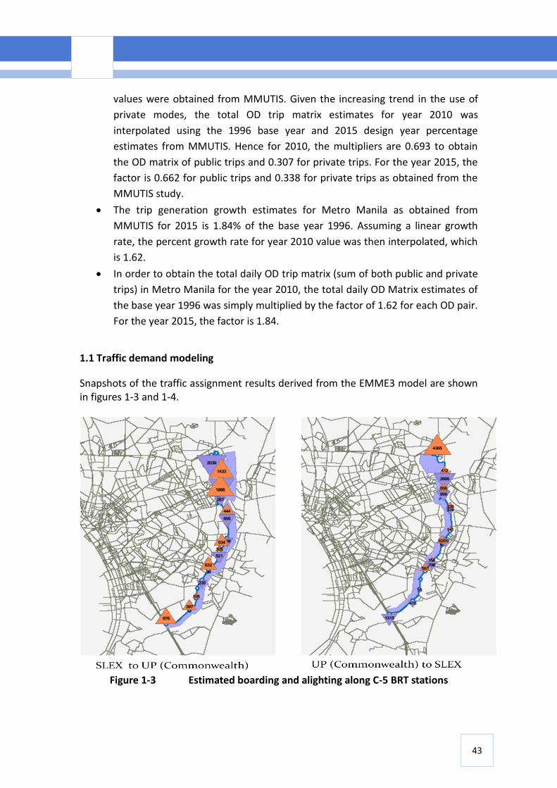
1.1 Traffic demand modelling 43 1.2 Users benefits calculation 45 1.3 Estimation of air pollutants and greenhouse gas emissions 45 1.4 Summary 46

2. Bangkok BRT 47 2.1 Traffic demand modelling 48 2.2 Users benefits calculation 49 2.3 Estimation of air pollutants and greenhouse gas emissions 50 2.4 Summary 51

4

1. Introduction

Efficient and modern transport systems are critical to development. But as the developing world urbanizes, the negative externalities from air pollution, on-road congestion, traffic accidents demonstrate the flaws in the conventional approach to transport planning. Simply building more roads and elevated expressways is neither sustainable nor desirable. Yet deviating from business-as-usual (BAU) requires not only a different set of transport choices but a different approach to transport planning. This “co-benefits approach” prioritizes transport projects that meet immediate development needs while addressing longer term climate change concerns. The transport sector accounts for more than two thirds of global oil consumption and emits 23% of energy related carbon dioxide (CO2) (IEA, 2009). This share is likely to increase due to rapid motorization in developing countries, especially countries in Asia. Road transport is the dominant producer of greenhouse gases (GHGs) from the transport sector, with cars accounting for almost half of domestic transport emissions by source. Policymakers in Asia hence are increasingly confronted with the following dilemma: how to reduce fossil fuel consumption thereby mitigating GHG emissions while improving energy security, mobility, road safety, and air quality? Mainstreaming co-benefits into transport planning is the first step to turning this challenge into an opportunity.

2. Taking a co-benefits approach in the transport sector: what, why and how?

A co-benefits approach capitalizes on synergies between current local problems (e.g. congestion, air pollution, etc.) and their future global consequence (climate change) by integrating multiple objectives into project planning. In addressing mobility, accessibility, road safety, air pollution and CO2 emissions in a holistic manner, a co-benefits approach not only can maximize benefits but minimize costs. The approach may further bring much needed funding to the transport sector if trends in international development finance and climate change negotiations continue to move in their current direction. It may also encourage policymakers to account for multiple benefits in the ex ante planning stage of a transport project in contrast to acknowledging ancillary or secondary benefits ex post. The Transport Co-benefits Guidelines (TCG) presents policymakers, practitioners and other stakeholders with a simple, intuitive tool to quantify co-benefits from transport projects in Asia. The TCG is intended to clarify the steps involved in estimating reductions in CO2 and conventional air pollutants as well time savings, vehicle operating costs, and accidents. It also aims to give different stakeholders a common understanding of how co-benefits were estimated. Throughout the TCG, the discussion

5

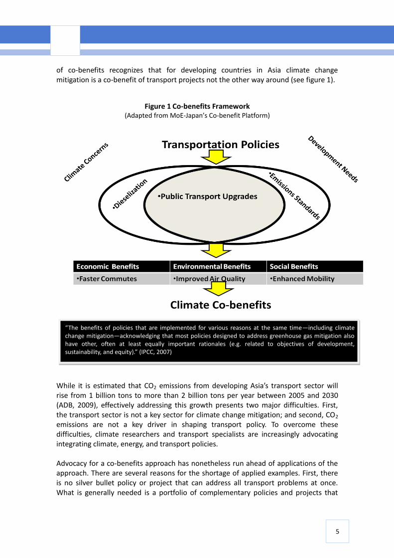
of co-benefits recognizes that for developing countries in Asia climate change mitigation is a co-benefit of transport projects not the other way around (see figure 1).

Figure 1 Co-benefits Framework (Adapted from MoE-Japan’s Co-benefit Platform)

While it is estimated that CO2 emissions from developing Asia’s transport sector will rise from 1 billion tons to more than 2 billion tons per year between 2005 and 2030 (ADB, 2009), effectively addressing this growth presents two major difficulties. First, the transport sector is not a key sector for climate change mitigation; and second, CO2 emissions are not a key driver in shaping transport policy. To overcome these difficulties, climate researchers and transport specialists are increasingly advocating integrating climate, energy, and transport policies. Advocacy for a co-benefits approach has nonetheless run ahead of applications of the approach. There are several reasons for the shortage of applied examples. First, there is no silver bullet policy or project that can address all transport problems at once. What is generally needed is a portfolio of complementary policies and projects that

“The benefits of policies that are implemented for various reasons at the same time—including climate change mitigation—acknowledging that most policies designed to address greenhouse gas mitigation also have other, often at least equally important rationales (e.g. related to objectives of development, sustainability, and equity).” (IPCC, 2007)

6

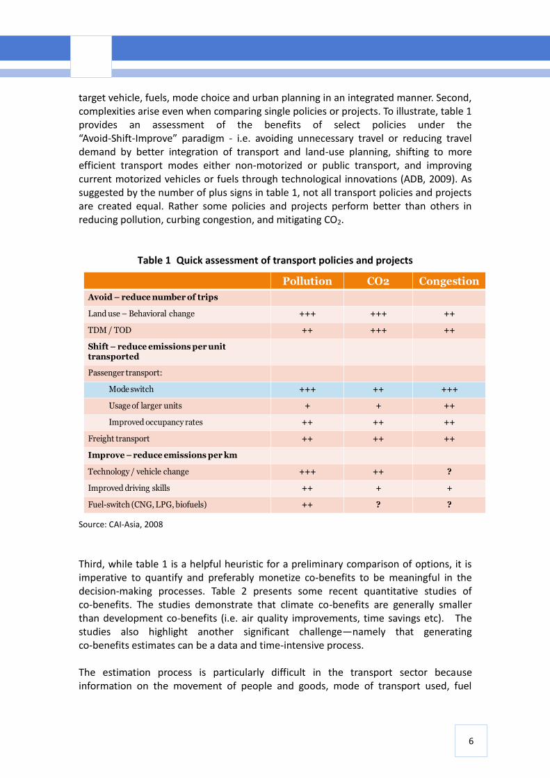
target vehicle, fuels, mode choice and urban planning in an integrated manner. Second, complexities arise even when comparing single policies or projects. To illustrate, table 1 provides an assessment of the benefits of select policies under the “Avoid-Shift-Improve” paradigm - i.e. avoiding unnecessary travel or reducing travel demand by better integration of transport and land-use planning, shifting to more efficient transport modes either non-motorized or public transport, and improving current motorized vehicles or fuels through technological innovations (ADB, 2009). As suggested by the number of plus signs in table 1, not all transport policies and projects are created equal. Rather some policies and projects perform better than others in reducing pollution, curbing congestion, and mitigating CO2.

Table 1 Quick assessment of transport policies and projects

Source: CAI-Asia, 2008

Third, while table 1 is a helpful heuristic for a preliminary comparison of options, it is imperative to quantify and preferably monetize co-benefits to be meaningful in the decision-making processes. Table 2 presents some recent quantitative studies of co-benefits. The studies demonstrate that climate co-benefits are generally smaller than development co-benefits (i.e. air quality improvements, time savings etc). The studies also highlight another significant challenge—namely that generating co-benefits estimates can be a data and time-intensive process. The estimation process is particularly difficult in the transport sector because information on the movement of people and goods, mode of transport used, fuel

Pollution CO2 Congestion

Avoid – reduce number of trips

Land use – Behavioral change +++ +++ ++

TDM / TOD ++ +++ ++

Shift – reduce emissions per unit transported

Passenger transport:

Mode switch +++ ++ +++

Usage of larger units + + ++

Improved occupancy rates ++ ++ ++

Freight transport ++ ++ ++

Improve –reduce emissions per km

Technology / vehicle change +++ ++ ?

Improved driving skills ++ + +

Fuel-switch (CNG, LPG, biofuels) ++ ? ?

7

consumption, and emission trends is often limited and fragmented. Further, though transport projects are typically required to conduct feasibility studies, economic impact assessment, and environmental impact analysis (especially projects funded by official development assistance (ODA) or multilateral banks), strong oversight is needed to ensure compliance. Finally and most importantly, government agencies often lack the human resources and technical training to become involved in the analysis of co-benefits. In addition to monitoring, an informed appreciation will be especially important during the conceptualization phase of the transport planning process.

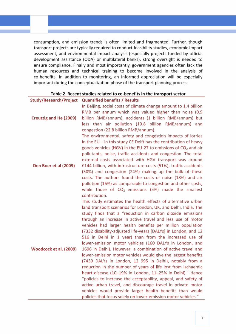
Table 2 Recent studies related to co-benefits in the transport sector

Study/Research/Project Quantified benefits / Results

Creutzig and He (2009)

In Beijing, social costs of climate change amount to 1.4 billion RMB per annum which was valued higher than noise (0.9 billion RMB/annum), accidents (1 billion RMB/annum) but less than air pollution (19.8 billion RMB/annum) and

congestion (22.8 billion RMB/annum).

Den Boer et al (2009)

The environmental, safety and congestion impacts of lorries in the EU – in this study CE Delft has the contribution of heavy goods vehicles (HGV) in the EU-27 to emissions of CO2 and air pollutants, noise, traffic accidents and congestion. The total external costs associated with HGV transport was around

€144 billion, with infrastructure costs (51%), traffic accidents (30%) and congestion (24%) making up the bulk of these costs. The authors found the costs of noise (18%) and air pollution (16%) as comparable to congestion and other costs, while those of CO2 emissions (5%) made the smallest contribution.

Woodcock et al. (2009)

This study estimates the health effects of alternative urban land transport scenarios for London, UK, and Delhi, India. The study finds that a “reduction in carbon dioxide emissions through an increase in active travel and less use of motor vehicles had larger health benefits per million population

(7332 disability-adjusted life-years [DALYs] in London, and 12 516 in Delhi in 1 year) than from the increased use of lower-emission motor vehicles (160 DALYs in London, and 1696 in Delhi). However, a combination of active travel and lower-emission motor vehicles would give the largest benefits (7439 DALYs in London, 12 995 in Delhi), notably from a reduction in the number of years of life lost from ischaemic heart disease (10–19% in London, 11–25% in Delhi).” Hence “policies to increase the acceptability, appeal, and safety of active urban travel, and discourage travel in private motor vehicles would provide larger health benefits than would

policies that focus solely on lower-emission motor vehicles.”

8

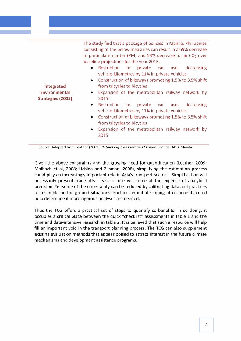
Integrated Environmental

Strategies (2005)

The study find that a package of policies in Manila, Philippines consisting of the below measures can result in a 69% decrease in particulate matter (PM) and 53% decrease for in CO2 over baseline projections for the year 2015.

Restriction to private car use, decreasing

vehicle-kilometres by 11% in private vehicles

Construction of bikeways promoting 1.5% to 3.5% shift from tricycles to bicycles

Expansion of the metropolitan railway network by

2015

Restriction to private car use, decreasing vehicle-kilometres by 11% in private vehicles

Construction of bikeways promoting 1.5% to 3.5% shift from tricycles to bicycles

Expansion of the metropolitan railway network by

2015

Source: Adapted from Leather (2009), Rethinking Transport and Climate Change. ADB. Manila.

Given the above constraints and the growing need for quantification (Leather, 2009; Maibach et al, 2008; Uchida and Zusman, 2008), simplifying the estimation process could play an increasingly important role in Asia’s transport sector. Simplification will necessarily present trade-offs - ease of use will come at the expense of analytical precision. Yet some of the uncertainty can be reduced by calibrating data and practices to resemble on-the-ground situations. Further, an initial scoping of co-benefits could help determine if more rigorous analyses are needed. Thus the TCG offers a practical set of steps to quantify co-benefits. In so doing, it occupies a critical place between the quick “checklist” assessments in table 1 and the time and data-intensive research in table 2. It is believed that such a resource will help fill an important void in the transport planning process. The TCG can also supplement existing evaluation methods that appear poised to attract interest in the future climate mechanisms and development assistance programs.

9

3. The future of co-benefits: the CDM, the post-2012 climate regime, and non-UNFCCC mechanisms

Co-benefits are not a new phenomenon. Since the 1990s, researchers have been applying energy models to estimate the ancillary air pollution and climate change benefits from policies and measures (Ayres and Walters, 1991). What is new is the growing interest in bringing this research to bear on actual sectoral policies and measures. The recent interest in practical application is particularly relevant for transport projects. In contrast to other sectors, transport projects often deliver sustainable development and GHG mitigation benefits. That transport projects generate these benefits corresponds with the Clean Development Mechanism’s (CDM) twin goals of providing low cost GHG mitigation opportunities and promoting sustainable development in host countries. This further fed expectations that CDM would play an important role in the transport sector when it was created in 2003. But since 2004 at the 10th Conference of Parties (COP 10) to the United Nations Framework Convention on Climate Change (UNFCCC) concerns have been raised about the “fit” between transport and the CDM (Sanchez, 2008). By COP 13, a report card on CDM paid more attention to the barriers than the potential for transport. Today the evidence of these barriers continues with only seven approved transport methodologies, three registered transport projects, and 0.4% of the total certified emission reduction strategies (CERs) from the transport sector. The disappointing performance of the CDM has led to several proposals to reform the CDM or the future climate regime or non-UNFCCC mechanisms. All three sets of reforms—to the CDM, to the future climate regime generally, and to international financing mechanisms outside the UNFCCC—involve accounting for a broader range of benefits than conventional appraisal frameworks.

Reforming the CDM-Several of the reform proposals concentrate on changing

the rules governing the CDM. These include suggestions to scale up the CDM

from the project to the policy or sectoral level. This would arguably help

transport projects because a larger scale mechanism would reduce the

transaction costs from measuring GHG reductions. Another set of proposals

calls for greater use the “first of its kind” principle that would allow some

project types to waive CDM additionality requirements. This was presumably

justified because transport projects were typically intended to achieve

development goals, thus it was difficult to demonstrate that a project was

additional to what would occur absent carbon finance.

10

Another set of potentially beneficial proposals for transport CDM focused on

promoting developmental co-benefits through “facilitative means.” The term

facilitative means referred to various forms of preferential treatment for

project activities with co-benefits, such as expedited processing times,

reductions in registration costs, or a relaxation of additionality rules (see table

3). These suggestions were not included the text of the Copenhagen Accord

(the main outcome of COP15) (UNFCCC, 2010) or the Cancun Agreement (the

main outcome COP16) (UNFCCC, 2010), and it remains to be seen if they will be

raised again in the lead up to COP 17. But their discussion suggests an interest

in quantifying co-benefits, especially for a comparably more flexible set of

mechanisms based on Nationally Appropriate Mitigation Actions (NAMAs).

Post-2012 Mechanisms: Nationally Appropriate Mitigation Actions (NAMAs)

and Measurable Reportable and Verifiable (MRV)-Among the most important

of these mechanisms are those that will provide technology, capacity building

and financial support to NAMAs. The acronym “NAMAs” was first used in the

Bali Action Plan—the 2007 agreement that laid a foundation for negotiating a

future climate change agreement. It has since been used in the Copenhagen

Accords and the Cancun Agreements. All three of these documents stipulate

that developing country parties would take NAMAs in the context of

sustainable development in exchange for financial, technology and capacity

building support in measurable, reportable, and verifiable (MRV) manner. The

interpretation of this text remains highly contested, but there is an emerging

consensus that developing countries could take pledge three different types of

NAMAs with corresponding differences in MRV:

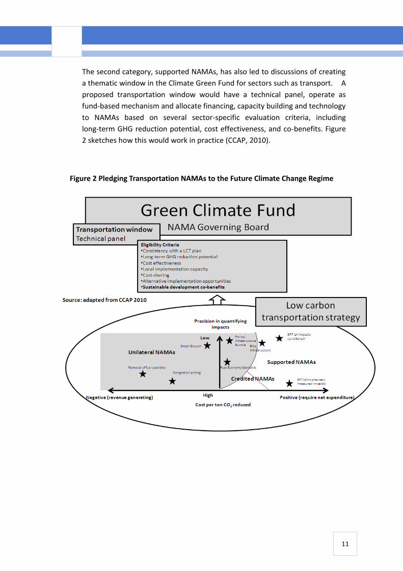
o Unilateral NAMAs - actions taken and financed independently by host

countries. These actions will be reported to the UNFCCC and

measured, reported and verified nationally with guidelines for

“international consultations and analysis (ICA).”

o Supported NAMAs -actions that would receive financial and other forms

of support from developed country parties. The Cancun agreements

suggest that this support will come from a Climate Green Fund under

the climate change regime. These NAMAs would be subject to MRV set

at the international level.

o Credited NAMAs - would receive financing from new crediting

mechanism under the UNFCCC. Again these NAMAs would be subject

to international MRV similar to the CDM.

11

The second category, supported NAMAs, has also led to discussions of creating

a thematic window in the Climate Green Fund for sectors such as transport. A

proposed transportation window would have a technical panel, operate as

fund-based mechanism and allocate financing, capacity building and technology

to NAMAs based on several sector-specific evaluation criteria, including

long-term GHG reduction potential, cost effectiveness, and co-benefits. Figure

2 sketches how this would work in practice (CCAP, 2010).

Figure 2 Pledging Transportation NAMAs to the Future Climate Change Regime

12

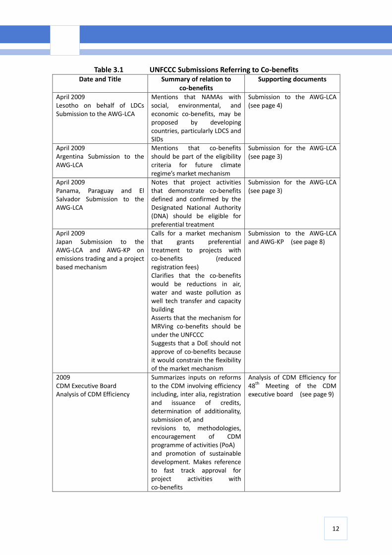
Table 3.1 UNFCCC Submissions Referring to Co-benefits Date and Title Summary of relation to

co-benefits Supporting documents

April 2009 Lesotho on behalf of LDCs Submission to the AWG-LCA

Mentions that NAMAs with social, environmental, and economic co-benefits, may be proposed by developing countries, particularly LDCS and SIDs

Submission to the AWG-LCA (see page 4)

April 2009 Argentina Submission to the AWG-LCA

Mentions that co-benefits should be part of the eligibility criteria for future climate regime’s market mechanism

Submission for the AWG-LCA (see page 3)

April 2009 Panama, Paraguay and El Salvador Submission to the AWG-LCA

Notes that project activities that demonstrate co-benefits defined and confirmed by the Designated National Authority (DNA) should be eligible for preferential treatment

Submission for the AWG-LCA (see page 3)

April 2009 Japan Submission to the AWG-LCA and AWG-KP on emissions trading and a project based mechanism

Calls for a market mechanism that grants preferential treatment to projects with co-benefits (reduced registration fees) Clarifies that the co-benefits would be reductions in air, water and waste pollution as well tech transfer and capacity building Asserts that the mechanism for MRVing co-benefits should be under the UNFCCC Suggests that a DoE should not approve of co-benefits because it would constrain the flexibility of the market mechanism

Submission to the AWG-LCA and AWG-KP (see page 8)

2009 CDM Executive Board Analysis of CDM Efficiency

Summarizes inputs on reforms to the CDM involving efficiency including, inter alia, registration and issuance of credits, determination of additionality, submission of, and revisions to, methodologies, encouragement of CDM programme of activities (PoA) and promotion of sustainable development. Makes reference to fast track approval for project activities with co-benefits

Analysis of CDM Efficiency for 48th Meeting of the CDM executive board (see page 9)

13

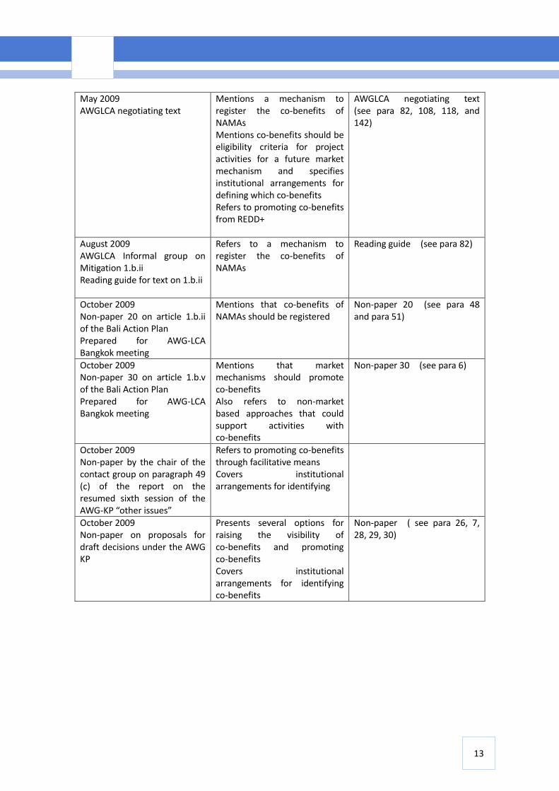
May 2009 AWGLCA negotiating text

Mentions a mechanism to register the co-benefits of NAMAs Mentions co-benefits should be eligibility criteria for project activities for a future market mechanism and specifies institutional arrangements for defining which co-benefits Refers to promoting co-benefits from REDD+

AWGLCA negotiating text (see para 82, 108, 118, and 142)

August 2009 AWGLCA Informal group on Mitigation 1.b.ii Reading guide for text on 1.b.ii

Refers to a mechanism to register the co-benefits of NAMAs

Reading guide (see para 82)

October 2009 Non-paper 20 on article 1.b.ii of the Bali Action Plan Prepared for AWG-LCA Bangkok meeting

Mentions that co-benefits of NAMAs should be registered

Non-paper 20 (see para 48 and para 51)

October 2009 Non-paper 30 on article 1.b.v of the Bali Action Plan Prepared for AWG-LCA Bangkok meeting

Mentions that market mechanisms should promote co-benefits Also refers to non-market based approaches that could support activities with co-benefits

Non-paper 30 (see para 6)

October 2009 Non-paper by the chair of the contact group on paragraph 49 (c) of the report on the resumed sixth session of the AWG-KP “other issues”

Refers to promoting co-benefits through facilitative means Covers institutional arrangements for identifying

October 2009 Non-paper on proposals for draft decisions under the AWG KP

Presents several options for raising the visibility of co-benefits and promoting co-benefits Covers institutional arrangements for identifying co-benefits

Non-paper ( see para 26, 7, 28, 29, 30)

14

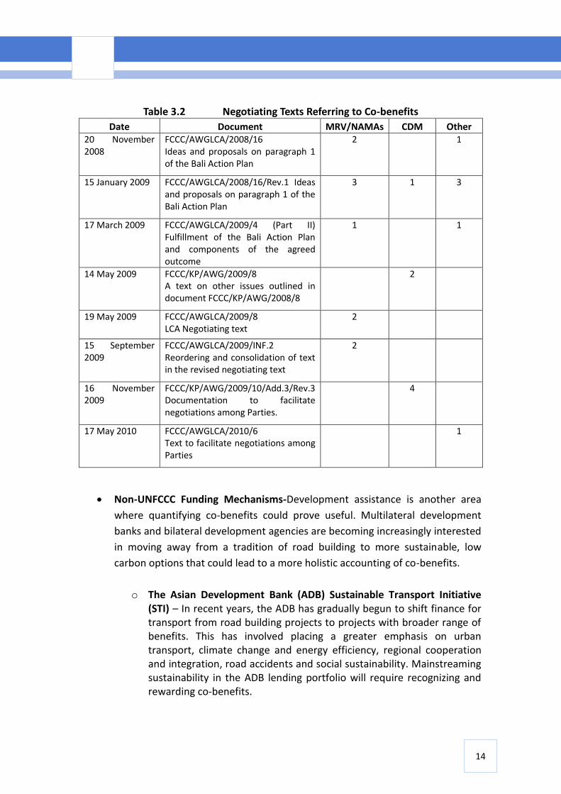
Table 3.2 Negotiating Texts Referring to Co-benefits

Date Document MRV/NAMAs CDM Other 20 November 2008

FCCC/AWGLCA/2008/16 Ideas and proposals on paragraph 1 of the Bali Action Plan

2 1

15 January 2009 FCCC/AWGLCA/2008/16/Rev.1 Ideas and proposals on paragraph 1 of the Bali Action Plan

3 1 3

17 March 2009 FCCC/AWGLCA/2009/4 (Part II) Fulfillment of the Bali Action Plan and components of the agreed outcome

1 1

14 May 2009 FCCC/KP/AWG/2009/8 A text on other issues outlined in document FCCC/KP/AWG/2008/8

2

19 May 2009 FCCC/AWGLCA/2009/8 LCA Negotiating text

2

15 September 2009

FCCC/AWGLCA/2009/INF.2 Reordering and consolidation of text in the revised negotiating text

2

16 November 2009

FCCC/KP/AWG/2009/10/Add.3/Rev.3 Documentation to facilitate negotiations among Parties.

4

17 May 2010 FCCC/AWGLCA/2010/6 Text to facilitate negotiations among Parties

1

Non-UNFCCC Funding Mechanisms-Development assistance is another area

where quantifying co-benefits could prove useful. Multilateral development

banks and bilateral development agencies are becoming increasingly interested

in moving away from a tradition of road building to more sustainable, low

carbon options that could lead to a more holistic accounting of co-benefits.

o The Asian Development Bank (ADB) Sustainable Transport Initiative (STI) – In recent years, the ADB has gradually begun to shift finance for transport from road building projects to projects with broader range of benefits. This has involved placing a greater emphasis on urban transport, climate change and energy efficiency, regional cooperation and integration, road accidents and social sustainability. Mainstreaming sustainability in the ADB lending portfolio will require recognizing and rewarding co-benefits.

15

o Climate Investment Funds (CIF) – In 2008, donors led by the World Bank pledged over US$6.1 billion to create climate investment funds to provide concessional finance for projects with global and local benefits. Of the two funds, the Climate Technology Fund (CTF) is increasingly concentrating on sustainable, low-carbon transport that could potentially have a transformative effect on the transport sector in developing countries.

Taking full advantage of these new developments will require not only changes in how the international community evaluates transport projects, but that policymakers in developing countries and transport practitioners have the expertise and tools to quantify co-benefits. The methodologies discussed herein intend to help build this capacity. By recognizing co-benefits – time savings, air quality improvement, health impacts, accident reduction, CO2 reduction – alternative transport projects will be given priority over conventional approach to building more roads and layers of elevated expressways.

16

4. Guide to quantifying transport co-benefits The TCG is intended for policymakers, private practitioners and specialists in the transport, climate, air pollution and urban planning sectors, as well as related funding institutions. The TCG helps to clarify the steps in estimating reductions in CO2 and conventional air pollutants as well time savings, vehicle operating costs, and accidents. It also aims to give different stakeholders a common understanding of how co-benefits were initially estimated and eventually measured, reported, and verified. The TCG is at this point focused on transport projects because they are a critical building block of transport policies. Future iterations may include methods for assessing policies. This section will guide the quantification of co-benefits. The section on quantification will revisit conventional cost-benefit analysis (CBA) to estimate and quantify time savings, vehicle operating costs savings, traffic accident reduction, and environmental benefits – local air pollution by measuring nitrogen oxide (NOx), particulate matter (PM) and carbon monoxide (CO); climate change mitigation by CO2. The methods in the TCG are based on Japan Research Institute’s (JRI) “Guidelines for the Evaluation of Road Investment Projects.” The decision to adapt JRI’s guidelines comes from a desire to build on existing capacity and experience. Rather than re-inventing the wheel, the TCG incorporates recent advances in estimating environment and climate impacts into well established assessment techniques. The JRI’s guidelines are already widely disseminated among transport experts, making it easier to integrate the updated and expanded environment and climate assessments into accepted techniques. This section of the TCG begins with steps for quantifying the benefits from time savings. It then moves to the benefits from vehicle operating costs. The third section focuses on road safety benefits. A final section concludes with environmental benefits, both urban air pollution and CO2. This guide provides initial values based on current available data. It is envisioned that users will update it accordingly, for their own purposes, as more data become available. To facilitate easy use and an open platform to reflect data updates, this guide comes with an Excel-based spreadsheet, the Transport Co-benefits Calculator. The spreadsheet follows the flow on how each co-benefit is calculated in the guide. Two BRT projects are shown as case study examples on how the guide can be used. Although the guide will not cover traffic demand forecasting, the results from any modelling software should be compatible with the methods to quantify co-benefits. The final results show the monetized co-benefits which could be meaningful in decision making processes considering both climate and developmental benefits.

17

4.1 Time savings

Basically travel time is monetized by simply multiplying travel time by the value of time. Value of time can be estimated in two ways – by resource value approach and behavioural value approach – wherein resource value means the marginal productivity of time with the assumption that a unit of time is used for production instead of driving while behavioural value means the user’s willingness to pay for a unit of time with the assumption that a unit of time can be used for others activities instead of driving.

4.1.1 Input data requirements

1. Traffic volume of each vehicle type – passenger car, bus, van, small truck, ordinary truck, motorcycle (with and without project)

2. Average travel time of each vehicle type (with and without project) 3. Value of time of each vehicle type

4.1.2 Formula

Benefit of travel time saving wo BTBTBT

Total Travel time cost (per year) 365j l

jijlijli TQBT

where, BT : Benefit of travel time saving

iBT : Total Travel time cost with/without project

ijlQ : traffic volume for j vehicle type on link l , with/without project

(vehicle/day)

ijlT : ave. travel time for j vehicle type on link l , with/without project (min）

j : value of time for j vehicle type (monetary unit/minute*vehicle)

i : wi with project, Oi without project, j : vehicle type

l : link

4.1.3 Estimating the value of time

The value of time depends on trip purpose, vehicle occupancy ratio, among other factors. Since neither traffic demand nor traffic volume is generally segmented by trip purpose but by vehicle type, the value of time is also estimated for each vehicle type. The value of working time per person is calculated based on the wage rate. However, the majority of trips are not work-related, but done on a traveler’s own time. The

18

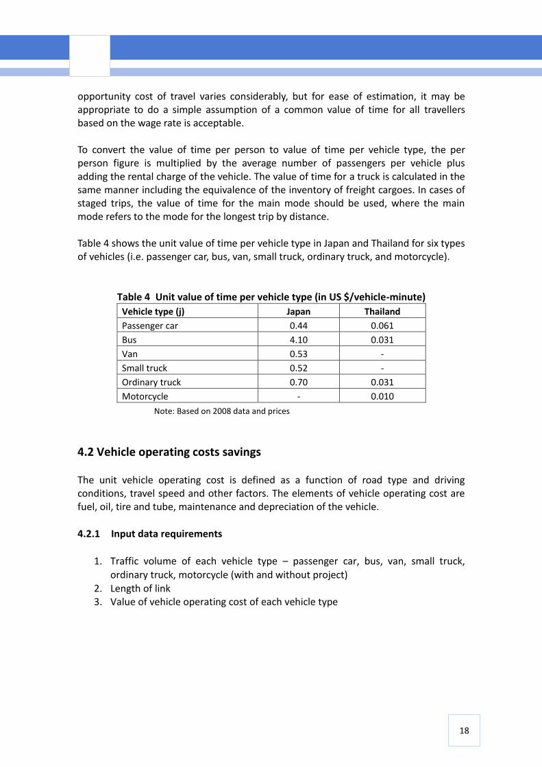
opportunity cost of travel varies considerably, but for ease of estimation, it may be appropriate to do a simple assumption of a common value of time for all travellers based on the wage rate is acceptable. To convert the value of time per person to value of time per vehicle type, the per person figure is multiplied by the average number of passengers per vehicle plus adding the rental charge of the vehicle. The value of time for a truck is calculated in the same manner including the equivalence of the inventory of freight cargoes. In cases of staged trips, the value of time for the main mode should be used, where the main mode refers to the mode for the longest trip by distance. Table 4 shows the unit value of time per vehicle type in Japan and Thailand for six types of vehicles (i.e. passenger car, bus, van, small truck, ordinary truck, and motorcycle).

Table 4 Unit value of time per vehicle type (in US $/vehicle-minute)

Vehicle type (j) Japan Thailand

Passenger car 0.44 0.061

Bus 4.10 0.031

Van 0.53 -

Small truck 0.52 -

Ordinary truck 0.70 0.031

Motorcycle - 0.010

Note: Based on 2008 data and prices

4.2 Vehicle operating costs savings The unit vehicle operating cost is defined as a function of road type and driving conditions, travel speed and other factors. The elements of vehicle operating cost are fuel, oil, tire and tube, maintenance and depreciation of the vehicle.


1. Traffic volume of each vehicle type – passenger car, bus, van, small truck, ordinary truck, motorcycle (with and without project)

2. Length of link 3. Value of vehicle operating cost of each vehicle type

19

4.2.2 Formula

Benefit of vehicle operating cost reduction wo BRBRBR

Total Travel time cost (per year) 365j l

jlijli LQBR

where, BR : Benefit of vehicle operating cost reduction

iBR : Total vehicle operating cost with/without project

ijlQ : traffic volume for j vehicle type on link l , with/without project

(vehicle/day)

lL : Link length of link l (km）

j : value of vehicle operating cost for j vehicle type (monetary

unit/minute*vehicle) i : wi with project, Oi without project, j : vehicle type

l : link

4.2.3 Estimating vehicle operating cost

The vehicle operating cost should be calculated for each OD pair by the following steps:

1. select the value of the unit vehicle operating cost for each link included in

the OD pair, according to travel speed, vehicle type and road type;

2. multiply the unit vehicle operating cost ($/vehicle･km) with traffic volume

on the link (vehicle･km) to obtain the vehicle operating cost for the link

volume (vehicle･km);

3. sum up the vehicle operating cost for each link over the links included for

each OD pair, and

4. divide the vehicle operating cost for the OD pair by the OD traffic volume so

as to obtain the vehicle operating cost per vehicle which is specific to each

OD pair.

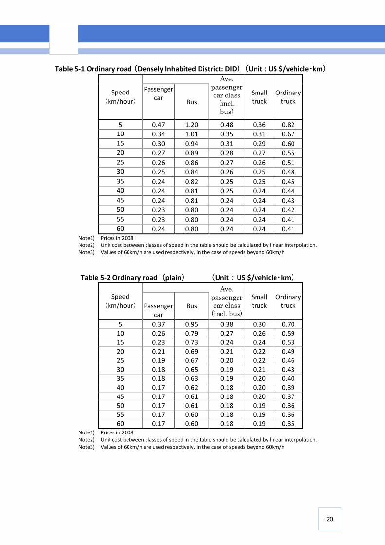
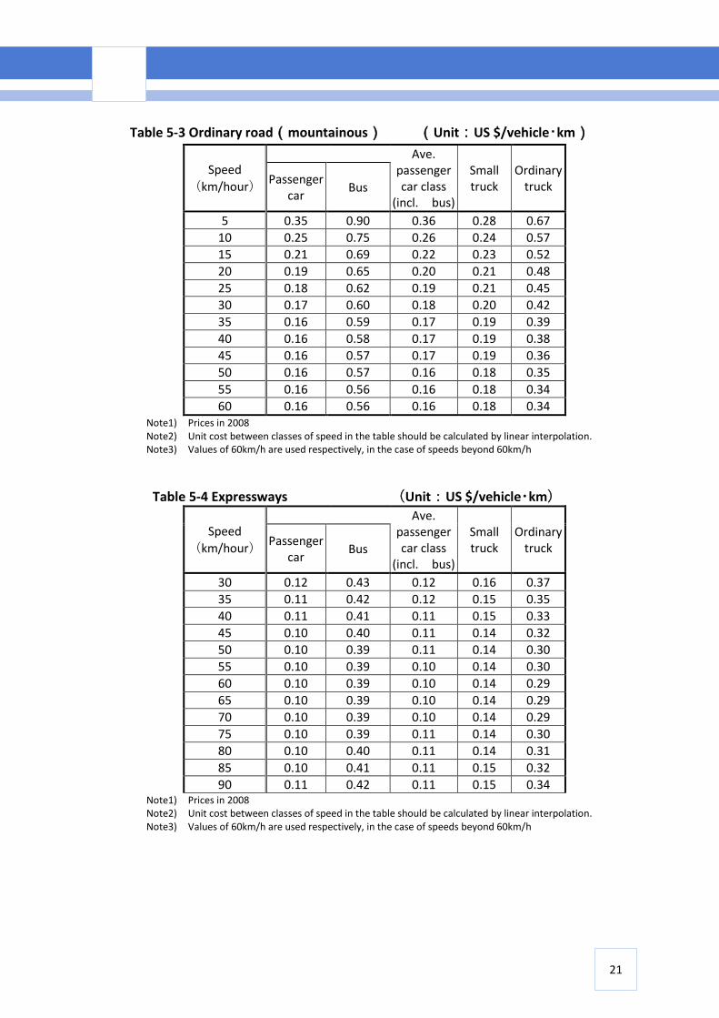
Japanese data on vehicle operating costs varies depending on the type of the road and terrain as shown in succeeding tables 5-1 to 5-4. These values can be used initially if there is no data available. Note that the denomination is in US $ converted from yen based on 2008 prices. Unit cost between classes of speed in the table should be calculated by linear interpolation. It is assumed that values corresponding to 60km/h are used in case of speeds beyond 60km/h.

20

Table 5-1 Ordinary road（Densely Inhabited District: DID）（Unit：US $/vehicle･km）

Speed

（km/hour）

Ave.

passenger

car class

(incl.

bus)

Small truck

Ordinary truck

Passenger car

Bus

5 0.47 1.20 0.48 0.36 0.82

10 0.34 1.01 0.35 0.31 0.67

15 0.30 0.94 0.31 0.29 0.60

20 0.27 0.89 0.28 0.27 0.55

25 0.26 0.86 0.27 0.26 0.51

30 0.25 0.84 0.26 0.25 0.48

35 0.24 0.82 0.25 0.25 0.45

40 0.24 0.81 0.25 0.24 0.44

45 0.24 0.81 0.24 0.24 0.43

50 0.23 0.80 0.24 0.24 0.42

55 0.23 0.80 0.24 0.24 0.41

60 0.24 0.80 0.24 0.24 0.41 Note1) Prices in 2008 Note2) Unit cost between classes of speed in the table should be calculated by linear interpolation. Note3) Values of 60km/h are used respectively, in the case of speeds beyond 60km/h

Table 5-2 Ordinary road（plain）（Unit：US $/vehicle･km）

Speed

（km/hour）

Ave.

passenger

car class

(incl. bus)

Small truck

Ordinary truck

Passenger

car Bus

5 0.37 0.95 0.38 0.30 0.70

10 0.26 0.79 0.27 0.26 0.59

15 0.23 0.73 0.24 0.24 0.53

20 0.21 0.69 0.21 0.22 0.49

25 0.19 0.67 0.20 0.22 0.46

30 0.18 0.65 0.19 0.21 0.43

35 0.18 0.63 0.19 0.20 0.40

40 0.17 0.62 0.18 0.20 0.39

45 0.17 0.61 0.18 0.20 0.37

50 0.17 0.61 0.18 0.19 0.36

55 0.17 0.60 0.18 0.19 0.36


21

Table 5-3 Ordinary road（mountainous）（Unit：US $/vehicle･km）

Speed

（km/hour）

Ave. passenger car class

(incl. bus)

Small truck

Ordinary truck

Passenger car

Bus

5 0.35 0.90 0.36 0.28 0.67

10 0.25 0.75 0.26 0.24 0.57

15 0.21 0.69 0.22 0.23 0.52

20 0.19 0.65 0.20 0.21 0.48

25 0.18 0.62 0.19 0.21 0.45

30 0.17 0.60 0.18 0.20 0.42

35 0.16 0.59 0.17 0.19 0.39

40 0.16 0.58 0.17 0.19 0.38

45 0.16 0.57 0.17 0.19 0.36

50 0.16 0.57 0.16 0.18 0.35

55 0.16 0.56 0.16 0.18 0.34


Table 5-4 Expressways （Unit：US $/vehicle･km）

Speed

（km/hour）

Ave. passenger car class

(incl. bus)

Small truck

Ordinary truck

Passenger car

Bus

30 0.12 0.43 0.12 0.16 0.37

35 0.11 0.42 0.12 0.15 0.35

40 0.11 0.41 0.11 0.15 0.33

45 0.10 0.40 0.11 0.14 0.32

50 0.10 0.39 0.11 0.14 0.30

55 0.10 0.39 0.10 0.14 0.30

60 0.10 0.39 0.10 0.14 0.29

65 0.10 0.39 0.10 0.14 0.29

70 0.10 0.39 0.10 0.14 0.29

75 0.10 0.39 0.11 0.14 0.30

80 0.10 0.40 0.11 0.14 0.31

85 0.10 0.41 0.11 0.15 0.32


22

4.3 Traffic safety benefits Traffic accident is a contingent event caused by many intricately inter-related factors. It is difficult to generalize whether measures that improve traffic flow enhance traffic safety. Most reports with data before and after a measure aimed at improving the flow of vehicles and pedestrians suggests these measures contribute to reducing the occurrence rate and damage from traffic accidents. The occurrence rate of traffic accident varies with factors such as road type, roadside type, road structure and characteristics of road traffic. The damage cost specified by types of traffic accident for each road section is also given as a function of the above-mentioned factors. Traffic accident statistics usually record the conditions of the accident point and the related road section, and the surrounding area. The statistics also record the following: the damage level; the numbers of casualties; fatal injuries; and minor injuries. Accidents are classified into vehicles mutually damaged, single vehicle damaged, pedestrian, bicycle, and so on. For material loss of vehicles, which does not include human injury, record of insurance payments for the vehicle damage can be a data source. Traffic volume at the accident point and the time required to clear the way determine the loss by traffic congestion. 4.3.1 Methodology

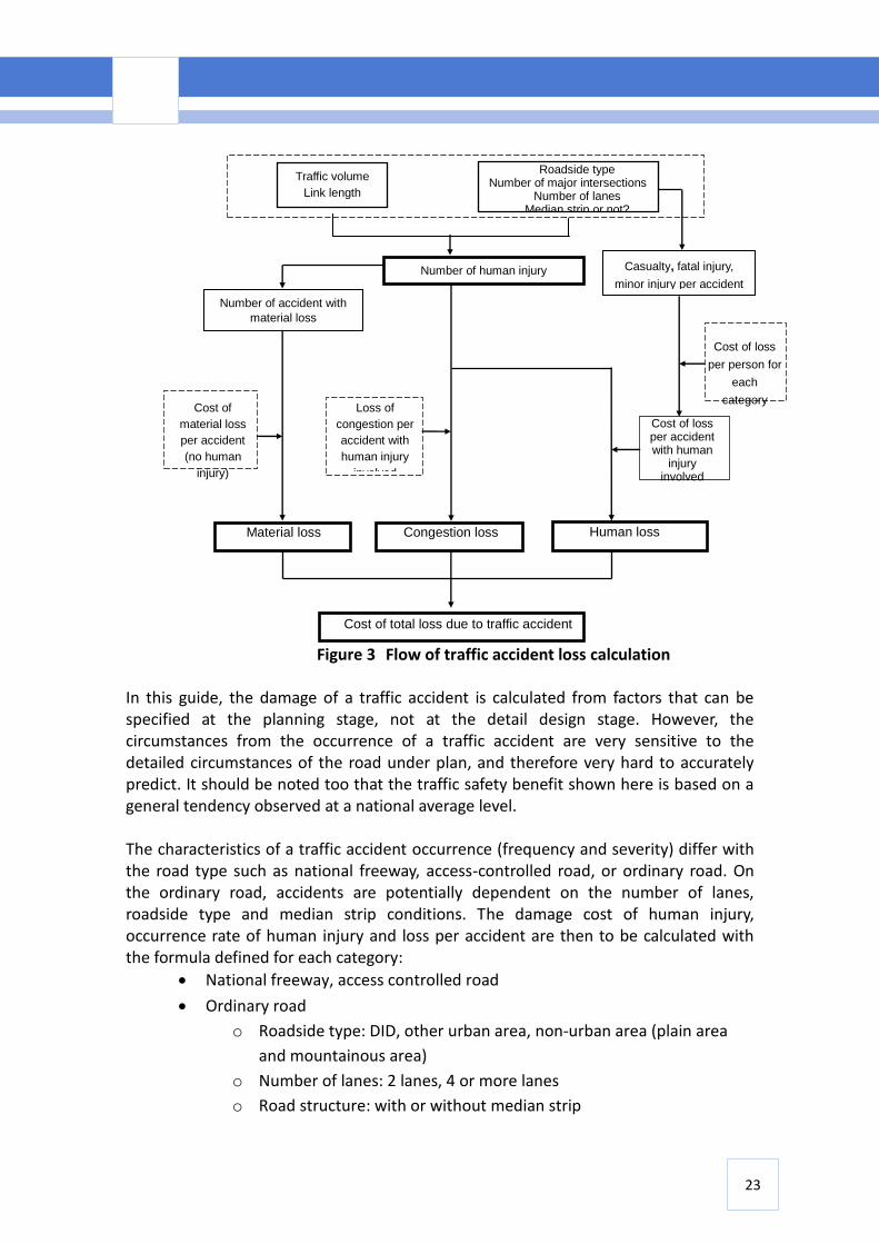
Generally, traffic safety benefit is calculated from the change in occurrence rate of accidents and damages incurred “with” and “without” any transport project or policy are introduced following the steps outlined in figure 3.

23

In this guide, the damage of a traffic accident is calculated from factors that can be specified at the planning stage, not at the detail design stage. However, the circumstances from the occurrence of a traffic accident are very sensitive to the detailed circumstances of the road under plan, and therefore very hard to accurately predict. It should be noted too that the traffic safety benefit shown here is based on a general tendency observed at a national average level. The characteristics of a traffic accident occurrence (frequency and severity) differ with the road type such as national freeway, access-controlled road, or ordinary road. On the ordinary road, accidents are potentially dependent on the number of lanes, roadside type and median strip conditions. The damage cost of human injury, occurrence rate of human injury and loss per accident are then to be calculated with the formula defined for each category:

National freeway, access controlled road

Ordinary road

o Roadside type: DID, other urban area, non-urban area (plain area

and mountainous area)

o Number of lanes: 2 lanes, 4 or more lanes

o Road structure: with or without median strip

Roadside type Number of major intersections

Number of lanes Median strip or not?

Congestion loss

Casualty, fatal injury,

minor injury per accident

Human loss

Material loss

Cost of loss

per person for

each

category

Cost of loss per accident with human

injury involved

Cost of

material loss

per accident

(no human

injury)

Loss of

congestion per

accident with

human injury

involved

Cost of total loss due to traffic accident

Traffic volume

Link length

Figure 3 Flow of traffic accident loss calculation

Number of human injury accidents

Number of accident with

material loss

24


1. Type of road 2. Type of roadside 3. Road structure – median strip condition 4. Number of lanes 5. Daily traffic volume (in 1,000 vehicles/day) 6. Length of link 7. Number of major intersections

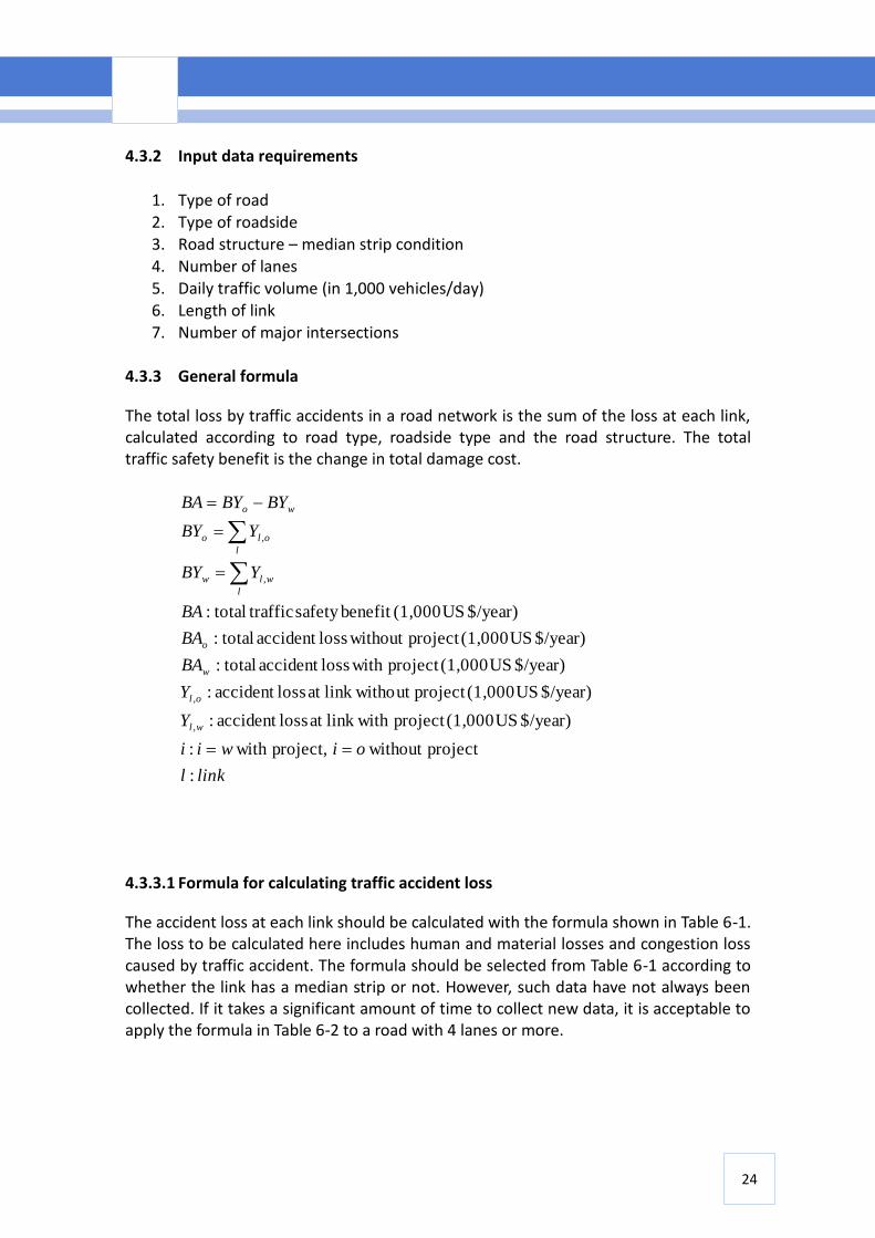
4.3.3 General formula

The total loss by traffic accidents in a road network is the sum of the loss at each link, calculated according to road type, roadside type and the road structure. The total traffic safety benefit is the change in total damage cost.

linkl

oiwii

Y

Y

BA

BA

BA

YBY

YBY

BYBYBA

wl

ol

w

o

l

wlw

l

olo

wo

:

project without project, with :

$/year) US(1,000project link with at lossaccident :　

$/year) US(1,000project ut link withoat lossaccident :

$/year) US(1,000project with lossaccident total:

$/year) US(1,000project without lossaccident total:　

$/year) US(1,000benefit safety traffictotal:

,

,

　

,

,

4.3.3.1 Formula for calculating traffic accident loss

The accident loss at each link should be calculated with the formula shown in Table 6-1. The loss to be calculated here includes human and material losses and congestion loss caused by traffic accident. The formula should be selected from Table 6-1 according to whether the link has a median strip or not. However, such data have not always been collected. If it takes a significant amount of time to collect new data, it is acceptable to apply the formula in Table 6-2 to a road with 4 lanes or more.

25

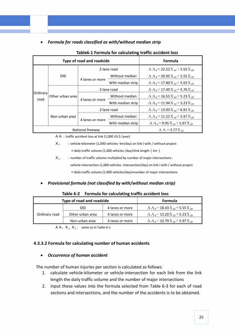
Formula for roads classified as with/without median strip

Table6-1 Formula for calculating traffic accident loss

Type of road and roadside Formula

Ordinary

road

DID

2-lane road ＡＡil＝22.52Ｘ1il＋5.55Ｘ2il

4 lanes or more Without median

strip

ＡＡil＝20.95Ｘ1il＋5.55Ｘ2il

With median strip ＡＡil＝17.80Ｘ1il＋5.55Ｘ2il

Other urban area



strip



Non-urban area



strip



National freeway ＡＡ＝3.77Ｘ1il

ＡＡ：traffic accident loss at link (1,000 US $ /year)

Ｘ1 ：vehicle-kilometer (1,000 vehicles･km/day) on link l with / without project

＝daily traffic volume (1,000 vehicles /day)×link length（km）

Ｘ2 ：number of traffic volume multiplied by number of major intersections :

vehicle-intersection (1,000 vehicles･intersection/day) on link l with / without project

＝daily traffic volume (1,000 vehicles/day)×number of major intersections

Provisional formula (not classified by with/without median strip)

Table 6-2 Formula for calculating traffic accident loss

Type of road and roadside Formula

Ordinary road

DID 4 lanes or more ＡＡil＝18.43Ｘ1il＋5.55Ｘ2il

Other urban area 4 lanes or more ＡＡil＝13.20Ｘ1il＋5.23Ｘ2il

Non-urban area 4 lanes or more ＡＡil＝10.79Ｘ1il＋5.97Ｘ2il

ＡＡ, Ｘ1, Ｘ2： same as in Table 6-1

4.3.3.2 Formula for calculating number of human accidents

Occurrence of human accident

The number of human injuries per section is calculated as follows: 1. calculate vehicle-kilometer or vehicle-intersection for each link from the link

length the daily traffic volume and the number of major intersections

2. input these values into the formula selected from Table 6-3 for each of road

sections and intersections, and the number of the accidents is to be obtained.

26

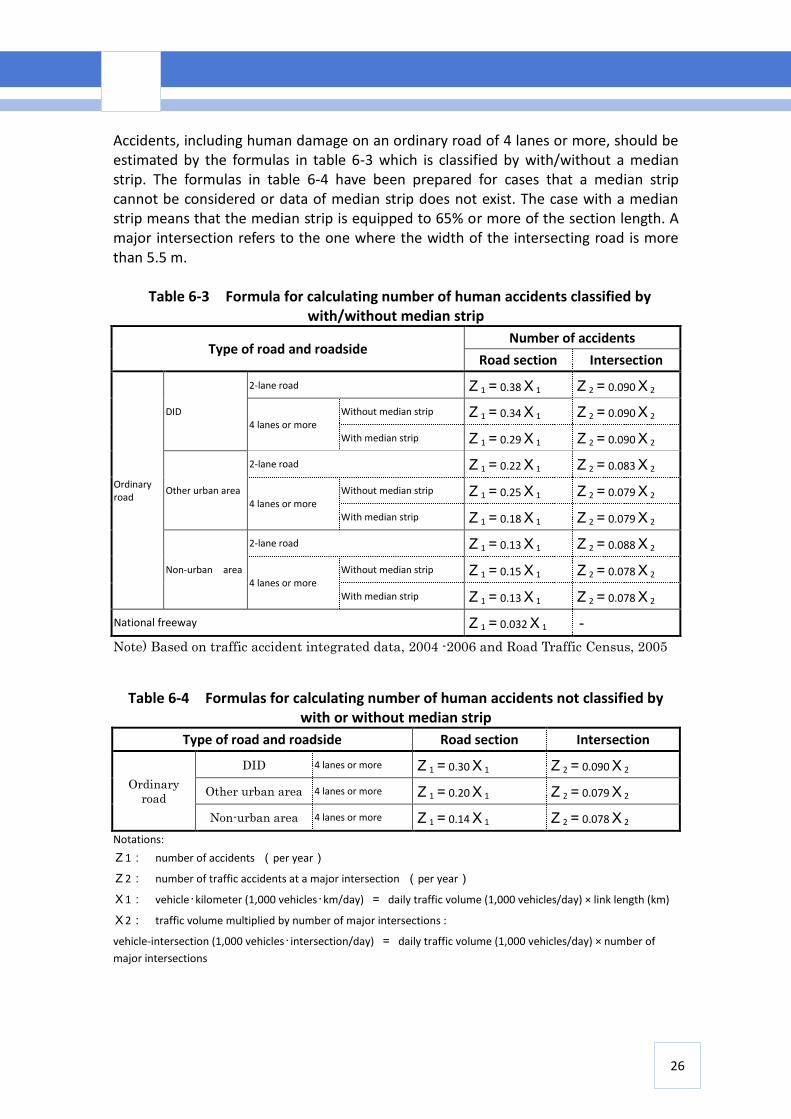
Accidents, including human damage on an ordinary road of 4 lanes or more, should be estimated by the formulas in table 6-3 which is classified by with/without a median strip. The formulas in table 6-4 have been prepared for cases that a median strip cannot be considered or data of median strip does not exist. The case with a median strip means that the median strip is equipped to 65% or more of the section length. A major intersection refers to the one where the width of the intersecting road is more than 5.5 m.

Table 6-3 Formula for calculating number of human accidents classified by with/without median strip

Type of road and roadside Number of accidents

Road section Intersection

Ordinary road

DID

2-lane road Ｚ1＝0.38Ｘ1 Ｚ2＝0.090Ｘ2

4 lanes or more Without median strip Ｚ1＝0.34Ｘ1 Ｚ2＝0.090Ｘ2

With median strip Ｚ1＝0.29Ｘ1 Ｚ2＝0.090Ｘ2

Other urban area

2-lane road Ｚ1＝0.22Ｘ1 Ｚ2＝0.083Ｘ2



Non-urban area

2-lane road Ｚ1＝0.13Ｘ1 Ｚ2＝0.088Ｘ2



National freeway Ｚ1＝0.032Ｘ1 －

Note) Based on traffic accident integrated data, 2004 -2006 and Road Traffic Census, 2005

Table 6-4 Formulas for calculating number of human accidents not classified by with or without median strip

Type of road and roadside Road section Intersection

Ordinary

road

DID 4 lanes or more Ｚ1＝0.30Ｘ1 Ｚ2＝0.090Ｘ2

Other urban area 4 lanes or more Ｚ1＝0.20Ｘ1 Ｚ2＝0.079Ｘ2

Non-urban area 4 lanes or more Ｚ1＝0.14Ｘ1 Ｚ2＝0.078Ｘ2

Notations:

Ｚ1： number of accidents （per year）

Ｚ2： number of traffic accidents at a major intersection （per year）

Ｘ1： vehicle･kilometer (1,000 vehicles･km/day) ＝ daily traffic volume (1,000 vehicles/day) × link length (km)

Ｘ2： traffic volume multiplied by number of major intersections :

vehicle-intersection (1,000 vehicles･intersection/day) ＝ daily traffic volume (1,000 vehicles/day) × number of

major intersections

27

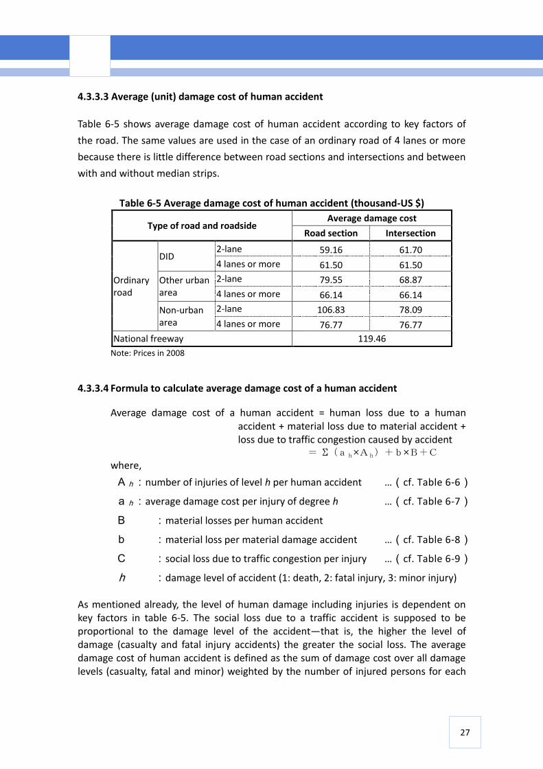
4.3.3.3 Average (unit) damage cost of human accident

Table 6-5 shows average damage cost of human accident according to key factors of

the road. The same values are used in the case of an ordinary road of 4 lanes or more

because there is little difference between road sections and intersections and between

with and without median strips.

Table 6-5 Average damage cost of human accident (thousand-US $)

Type of road and roadside Average damage cost

Road section Intersection

Ordinary road

DID 2-lane 59.16 61.70

4 lanes or more 61.50 61.50

Other urban area

2-lane 79.55 68.87


Non-urban area

2-lane 106.83 78.09


National freeway 119.46

Note: Prices in 2008

4.3.3.4 Formula to calculate average damage cost of a human accident

Average damage cost of a human accident = human loss due to a human accident + material loss due to material accident + loss due to traffic congestion caused by accident

＝ Σ（ａｈ×Ａｈ）＋ｂ×Ｂ＋Ｃ

where,

Ａｈ：number of injuries of level h per human accident …（cf. Table 6-6）

ａｈ：average damage cost per injury of degree h …（cf. Table 6-7）

Ｂ：material losses per human accident

ｂ：material loss per material damage accident …（cf. Table 6-8）

Ｃ：social loss due to traffic congestion per injury …（cf. Table 6-9）

ｈ：damage level of accident (1: death, 2: fatal injury, 3: minor injury)

As mentioned already, the level of human damage including injuries is dependent on key factors in table 6-5. The social loss due to a traffic accident is supposed to be proportional to the damage level of the accident—that is, the higher the level of damage (casualty and fatal injury accidents) the greater the social loss. The average damage cost of human accident is defined as the sum of damage cost over all damage levels (casualty, fatal and minor) weighted by the number of injured persons for each

28

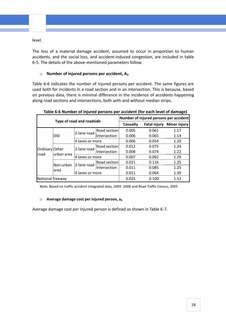
level. The loss of a material damage accident, assumed to occur in proportion to human accidents, and the social loss, and accident-induced congestion, are included in table 6-5. The details of the above-mentioned parameters follow.

o Number of injured persons per accident, Ah

Table 6-6 indicates the number of injured persons per accident. The same figures are used both for incidents in a road section and in an intersection. This is because, based on previous data, there is minimal difference in the incidence of accidents happening along road sections and intersections, both with and without median strips.

Table 6-6 Number of injured persons per accident (for each level of damage)

Type of road and roadside Number of injured persons per accident

Casualty Fatal injury Minor injury

Ordinary road

DID 2-lane road

Road section 0.005 0.061 1.17

Intersection 0.006 0.065 1.14

4 lanes or more 0.006 0.054 1.20

Other urban area

2-lane road Road section 0.012 0.075 1.24


4 lanes or more 0.007 0.062 1.29

Non-urban area

2-lane road Road section 0.021 0.116 1.25


4 lanes or more 0.011 0.064 1.30

National freeway 0.025 0.100 1.52

Note: Based on traffic accident integrated data, 2004 -2006 and Road Traffic Census, 2005

o Average damage cost per injured person, ah

Average damage cost per injured person is defined as shown in Table 6-7.

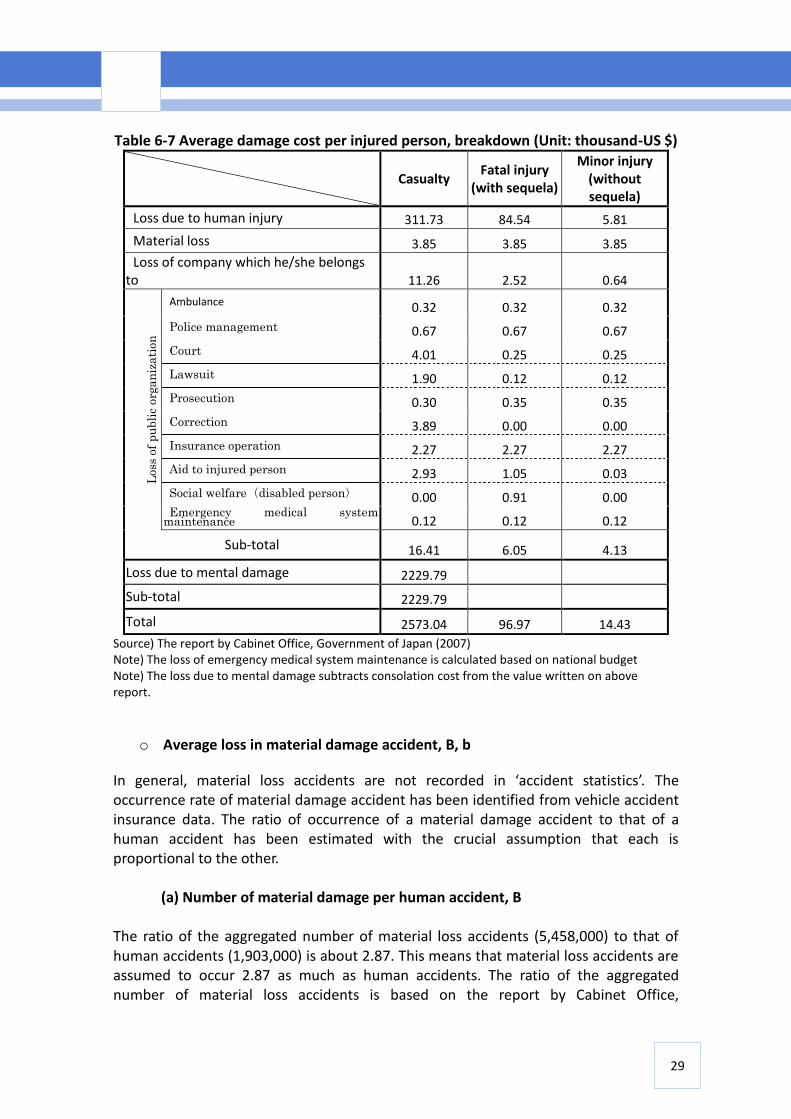
29

Table 6-7 Average damage cost per injured person, breakdown (Unit: thousand-US $)

Casualty Fatal injury

(with sequela)

Minor injury (without sequela)

Loss due to human injury 311.73 84.54 5.81

Material loss 3.85 3.85 3.85

Loss of company which he/she belongs to 11.26 2.52 0.64

Ambulance 0.32 0.32 0.32

Police management 0.67 0.67 0.67

Court 4.01 0.25 0.25

Lawsuit 1.90 0.12 0.12

Prosecution 0.30 0.35 0.35

Correction 3.89 0.00 0.00

Insurance operation 2.27 2.27 2.27

Aid to injured person 2.93 1.05 0.03

Social welfare（disabled person） 0.00 0.91 0.00

Emergency medical system maintenance 0.12 0.12 0.12

Sub-total 16.41 6.05 4.13

Loss due to mental damage 2229.79

Sub-total 2229.79

Total 2573.04 96.97 14.43

Source) The report by Cabinet Office, Government of Japan (2007) Note) The loss of emergency medical system maintenance is calculated based on national budget Note) The loss due to mental damage subtracts consolation cost from the value written on above report.

o Average loss in material damage accident, B, b

In general, material loss accidents are not recorded in ‘accident statistics’. The occurrence rate of material damage accident has been identified from vehicle accident insurance data. The ratio of occurrence of a material damage accident to that of a human accident has been estimated with the crucial assumption that each is proportional to the other.

(a) Number of material damage per human accident, B

The ratio of the aggregated number of material loss accidents (5,458,000) to that of human accidents (1,903,000) is about 2.87. This means that material loss accidents are assumed to occur 2.87 as much as human accidents. The ratio of the aggregated number of material loss accidents is based on the report by Cabinet Office,

Loss

of

pu

bli

c org

an

iza

tion

30

Government of Japan (2007).

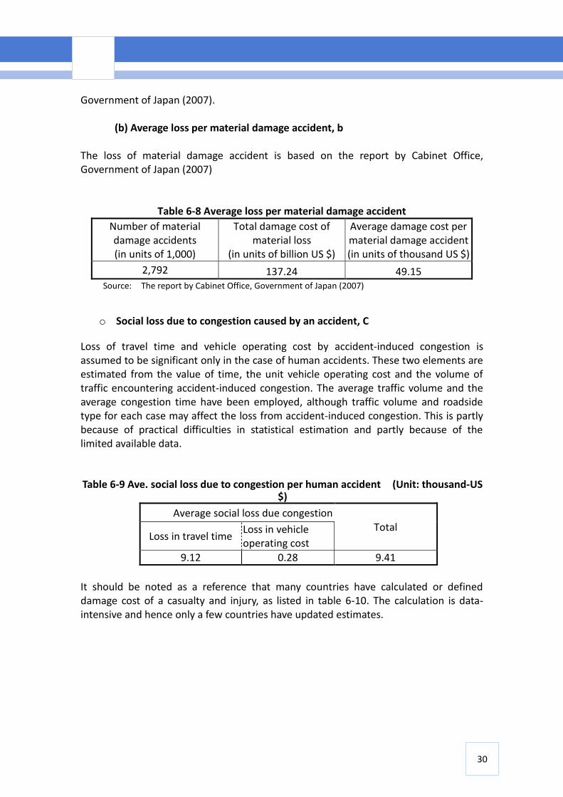
(b) Average loss per material damage accident, b

The loss of material damage accident is based on the report by Cabinet Office, Government of Japan (2007)

Table 6-8 Average loss per material damage accident

Number of material damage accidents (in units of 1,000)

Total damage cost of material loss

(in units of billion US $)

Average damage cost per material damage accident (in units of thousand US $)

2,792 137.24 49.15 Source: The report by Cabinet Office, Government of Japan (2007) o Social loss due to congestion caused by an accident, C

Loss of travel time and vehicle operating cost by accident-induced congestion is assumed to be significant only in the case of human accidents. These two elements are estimated from the value of time, the unit vehicle operating cost and the volume of traffic encountering accident-induced congestion. The average traffic volume and the average congestion time have been employed, although traffic volume and roadside type for each case may affect the loss from accident-induced congestion. This is partly because of practical difficulties in statistical estimation and partly because of the limited available data. Table 6-9 Ave. social loss due to congestion per human accident (Unit: thousand-US

$)

Average social loss due congestion Total

Loss in travel time Loss in vehicle operating cost

9.12 0.28 9.41

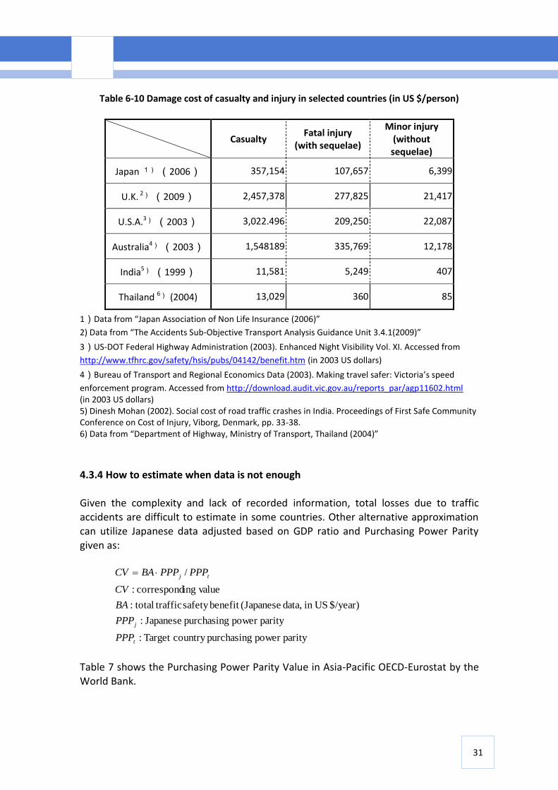
It should be noted as a reference that many countries have calculated or defined damage cost of a casualty and injury, as listed in table 6-10. The calculation is data- intensive and hence only a few countries have updated estimates.

31

Table 6-10 Damage cost of casualty and injury in selected countries (in US $/person)

Casualty Fatal injury

(with sequelae)

Minor injury (without sequelae)

Japan １）（2006） 357,154 107,657 6,399

U.K. 2）（2009） 2,457,378 277,825 21,417

U.S.A.3）（2003） 3,022.496 209,250 22,087

Australia4）（2003） 1,548189 335,769 12,178

India5）（1999） 11,581 5,249 407

Thailand 6） (2004) 13,029 360 85

1）Data from “Japan Association of Non Life Insurance (2006)”

2) Data from “The Accidents Sub-Objective Transport Analysis Guidance Unit 3.4.1(2009)”

3）US-DOT Federal Highway Administration (2003). Enhanced Night Visibility Vol. XI. Accessed from

http://www.tfhrc.gov/safety/hsis/pubs/04142/benefit.htm (in 2003 US dollars)

4）Bureau of Transport and Regional Economics Data (2003). Making travel safer: Victoria’s speed

enforcement program. Accessed from http://download.audit.vic.gov.au/reports_par/agp11602.html (in 2003 US dollars) 5) Dinesh Mohan (2002). Social cost of road traffic crashes in India. Proceedings of First Safe Community Conference on Cost of Injury, Viborg, Denmark, pp. 33-38. 6) Data from “Department of Highway, Ministry of Transport, Thailand (2004)”

4.3.4 How to estimate when data is not enough Given the complexity and lack of recorded information, total losses due to traffic accidents are difficult to estimate in some countries. Other alternative approximation can utilize Japanese data adjusted based on GDP ratio and Purchasing Power Parity

given as:

paritypower purchasingcountry Target :

paritypower purchasing Japanese:

$/year) in US data, (Japanesebenefit safety traffictotal:

value　ingcorrespond:

/

t

j

tj

PPP

PPP

BA

CV

PPPPPPBACV

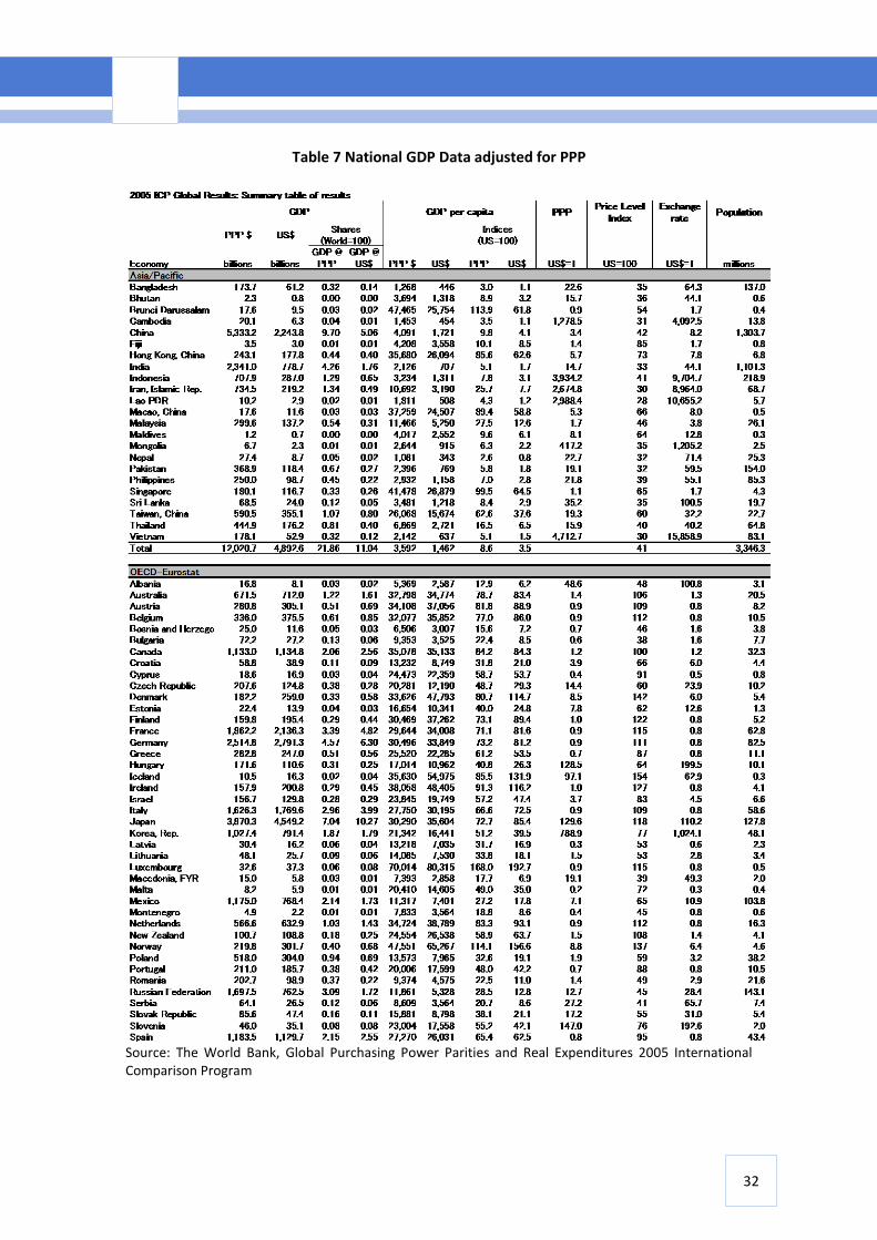
Table 7 shows the Purchasing Power Parity Value in Asia-Pacific OECD-Eurostat by the World Bank.

http://www.tfhrc.gov/safety/hsis/pubs/04142/benefit.htm

http://download.audit.vic.gov.au/reports_par/agp11602.html

32

Table 7 National GDP Data adjusted for PPP

Source: The World Bank, Global Purchasing Power Parities and Real Expenditures 2005 International Comparison Program

33

4.4 Environmental benefits

Transport projects may affect the environment, contributing to climate change, air pollution, noise, vibration, land use and ecological changes. One of the environmental benefits gained from transport projects is climate change mitigation by reducing greenhouse gases such as CO2. Some transport projects also have the potential to reduce conventional air pollutants such as nitrogen oxide (NOx) and particulate matter (PM), and to improve local air quality, therefore reducing air pollution and related health impacts. Environmental benefits from transport projects can be estimated with the following steps:

Step 1: Estimation of emissions Step 2: Calculation of damage cost

The effects of traffic on the environment vary with the composition of vehicle type and travel speed. The distribution of inhabitants in impact areas differs between roadside types. In converting the environmental impacts to monetary values, the impacts should be calculated for every roadside type.


1. Vehicle type - classified into small vehicle (i.e. privately owned passenger car and small truck) and large vehicle (i.e. bus and ordinary truck)

2. Vehicle speed - average travel speed for each link obtained from the results of traffic assignment.

3. Roadside type - classified into four types which have been already adopted in the Road Traffic Census: DID, other urban area, non-urban area (plain) and non-urban area (mountainous). Note: the sum of link length over these four roadside types should equal the total route length of the network.

4. Emission factor for each vehicle type

5. Average daily traffic volume of each vehicle type 6. Length of link 7. Fuel economy for each vehicle type at average speed 8. Net calorific value of fuel 9. Emission factor for fuel

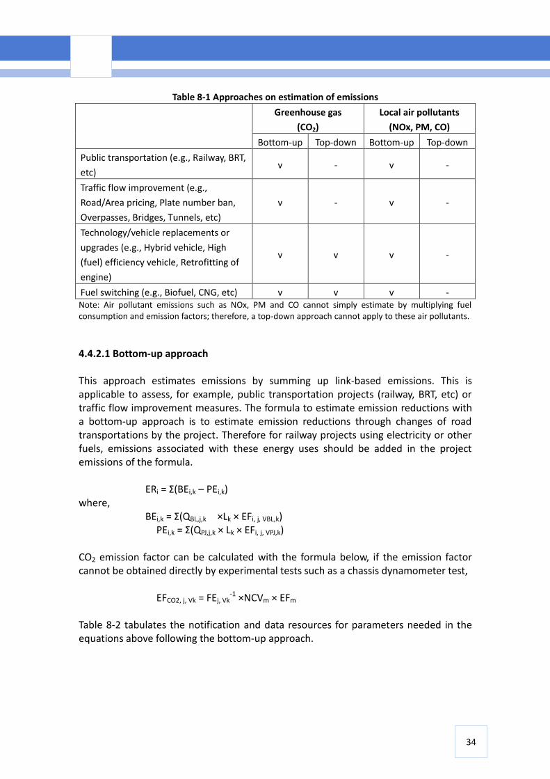
4.4.2 Estimation of emissions There are two approaches, depending on project types, to estimate CO2 and air pollutant emissions as shown in table 8-1.

34

Table 8-1 Approaches on estimation of emissions

Greenhouse gas

(CO2)

Local air pollutants

(NOx, PM, CO)

Bottom-up Top-down Bottom-up Top-down

Public transportation (e.g., Railway, BRT,

etc) v - v -

Traffic flow improvement (e.g.,

Road/Area pricing, Plate number ban,

Overpasses, Bridges, Tunnels, etc)

v - v -

Technology/vehicle replacements or

upgrades (e.g., Hybrid vehicle, High

(fuel) efficiency vehicle, Retrofitting of

engine)

v v v -

Fuel switching (e.g., Biofuel, CNG, etc) v v v - Note: Air pollutant emissions such as NOx, PM and CO cannot simply estimate by multiplying fuel consumption and emission factors; therefore, a top-down approach cannot apply to these air pollutants.

4.4.2.1 Bottom-up approach This approach estimates emissions by summing up link-based emissions. This is applicable to assess, for example, public transportation projects (railway, BRT, etc) or traffic flow improvement measures. The formula to estimate emission reductions with a bottom-up approach is to estimate emission reductions through changes of road transportations by the project. Therefore for railway projects using electricity or other fuels, emissions associated with these energy uses should be added in the project emissions of the formula.

ERi = Σ(BEi,k – PEi,k) where,

BEi,k = Σ(QBL,j,k ×Lk × EFi, j, VBL,k) PEi,k = Σ(QPJ,j,k × Lk × EFi, j, VPJ,k) CO2 emission factor can be calculated with the formula below, if the emission factor cannot be obtained directly by experimental tests such as a chassis dynamometer test, EFCO2, j, Vk = FEj, Vk

-1 ×NCVm × EFm Table 8-2 tabulates the notification and data resources for parameters needed in the equations above following the bottom-up approach.

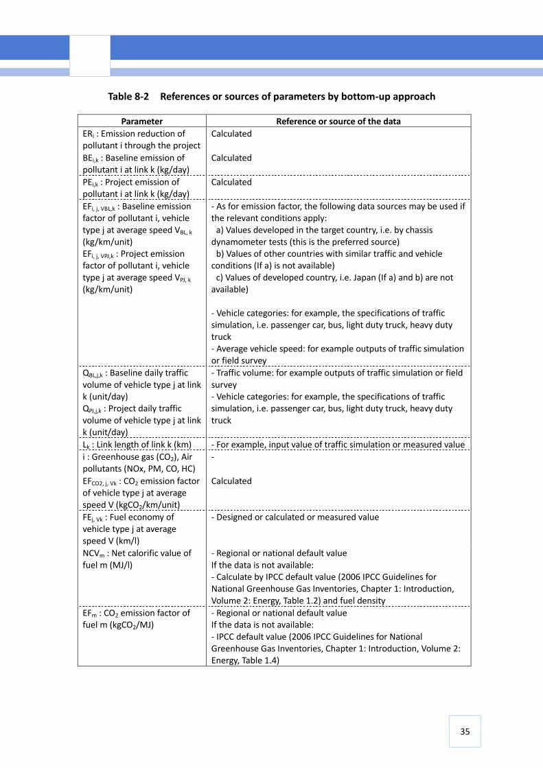
35

Table 8-2 References or sources of parameters by bottom-up approach

Parameter Reference or source of the data

ERi : Emission reduction of pollutant i through the project

Calculated

BEi,k : Baseline emission of pollutant i at link k (kg/day)

Calculated

PEi,k : Project emission of pollutant i at link k (kg/day)

Calculated

EFi, j, VBL,k : Baseline emission factor of pollutant i, vehicle type j at average speed VBL, k (kg/km/unit) EFi, j, VPJ,k : Project emission factor of pollutant i, vehicle type j at average speed VPJ, k (kg/km/unit)

- As for emission factor, the following data sources may be used if the relevant conditions apply: a) Values developed in the target country, i.e. by chassis dynamometer tests (this is the preferred source) b) Values of other countries with similar traffic and vehicle conditions (If a) is not available) c) Values of developed country, i.e. Japan (If a) and b) are not available) - Vehicle categories: for example, the specifications of traffic simulation, i.e. passenger car, bus, light duty truck, heavy duty truck - Average vehicle speed: for example outputs of traffic simulation or field survey

QBL,j,k : Baseline daily traffic volume of vehicle type j at link k (unit/day) QPJ,j,k : Project daily traffic volume of vehicle type j at link k (unit/day)

- Traffic volume: for example outputs of traffic simulation or field survey - Vehicle categories: for example, the specifications of traffic simulation, i.e. passenger car, bus, light duty truck, heavy duty truck

Lk : Link length of link k (km) - For example, input value of traffic simulation or measured value

i : Greenhouse gas (CO2), Air pollutants (NOx, PM, CO, HC)

-

EFCO2, j, Vk : CO2 emission factor of vehicle type j at average speed V (kgCO2/km/unit)

Calculated

FEj, Vk : Fuel economy of vehicle type j at average speed V (km/l)

- Designed or calculated or measured value

NCVm : Net calorific value of fuel m (MJ/l)

- Regional or national default value If the data is not available: - Calculate by IPCC default value (2006 IPCC Guidelines for National Greenhouse Gas Inventories, Chapter 1: Introduction, Volume 2: Energy, Table 1.2) and fuel density

EFm : CO2 emission factor of fuel m (kgCO2/MJ)

- Regional or national default value If the data is not available: - IPCC default value (2006 IPCC Guidelines for National Greenhouse Gas Inventories, Chapter 1: Introduction, Volume 2: Energy, Table 1.4)

36

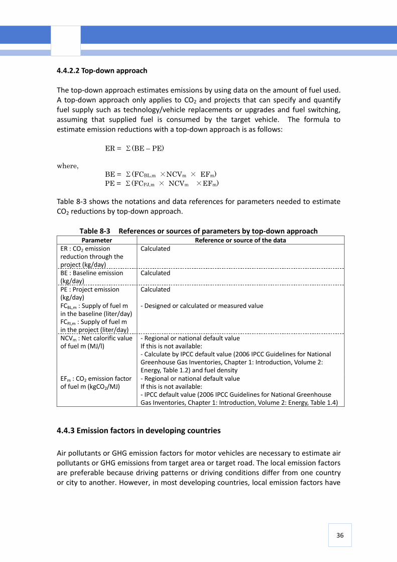
4.4.2.2 Top-down approach The top-down approach estimates emissions by using data on the amount of fuel used. A top-down approach only applies to CO2 and projects that can specify and quantify fuel supply such as technology/vehicle replacements or upgrades and fuel switching, assuming that supplied fuel is consumed by the target vehicle. The formula to estimate emission reductions with a top-down approach is as follows:

ER = Σ(BE – PE)

where,

BE = Σ(FCBL,m ×NCVm × EFm)

PE = Σ(FCPJ,m × NCVm ×EFm)

Table 8-3 shows the notations and data references for parameters needed to estimate CO2 reductions by top-down approach.

Table 8-3 References or sources of parameters by top-down approach Parameter Reference or source of the data

ER : CO2 emission reduction through the project (kg/day)

Calculated

BE : Baseline emission (kg/day)

Calculated

PE : Project emission (kg/day)

Calculated

FCBL,m : Supply of fuel m in the baseline (liter/day) FCPJ,m : Supply of fuel m in the project (liter/day)

- Designed or calculated or measured value

NCVm : Net calorific value of fuel m (MJ/l)

- Regional or national default value If this is not available: - Calculate by IPCC default value (2006 IPCC Guidelines for National Greenhouse Gas Inventories, Chapter 1: Introduction, Volume 2: Energy, Table 1.2) and fuel density

EFm : CO2 emission factor of fuel m (kgCO2/MJ)

- Regional or national default value If this is not available: - IPCC default value (2006 IPCC Guidelines for National Greenhouse Gas Inventories, Chapter 1: Introduction, Volume 2: Energy, Table 1.4)

4.4.3 Emission factors in developing countries

Air pollutants or GHG emission factors for motor vehicles are necessary to estimate air pollutants or GHG emissions from target area or target road. The local emission factors are preferable because driving patterns or driving conditions differ from one country or city to another. However, in most developing countries, local emission factors have

37

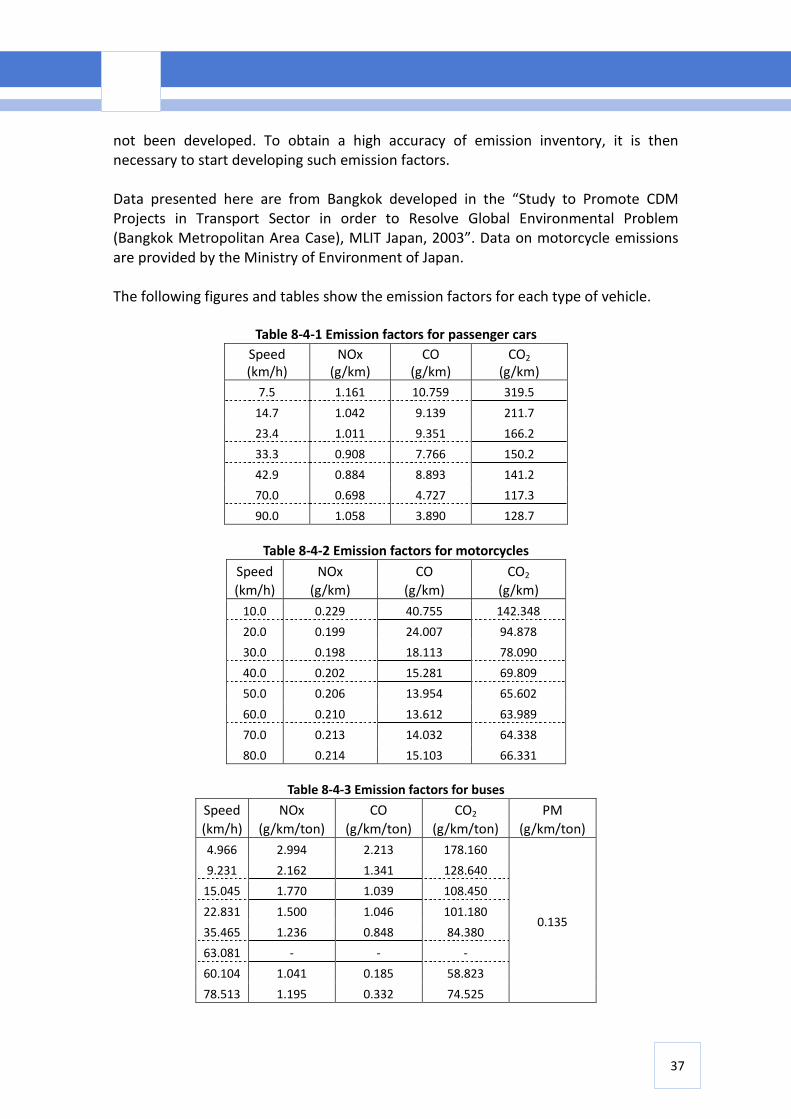
not been developed. To obtain a high accuracy of emission inventory, it is then necessary to start developing such emission factors. Data presented here are from Bangkok developed in the “Study to Promote CDM Projects in Transport Sector in order to Resolve Global Environmental Problem (Bangkok Metropolitan Area Case), MLIT Japan, 2003”. Data on motorcycle emissions are provided by the Ministry of Environment of Japan. The following figures and tables show the emission factors for each type of vehicle.

Table 8-4-1 Emission factors for passenger cars

Speed (km/h)

NOx (g/km)

CO (g/km)

CO2 (g/km)

7.5 1.161 10.759 319.5

14.7 1.042 9.139 211.7

23.4 1.011 9.351 166.2

33.3 0.908 7.766 150.2

42.9 0.884 8.893 141.2

70.0 0.698 4.727 117.3

90.0 1.058 3.890 128.7

Table 8-4-2 Emission factors for motorcycles

Speed

(km/h)

NOx

(g/km)

CO

(g/km)

CO2

(g/km)

10.0 0.229 40.755 142.348

20.0 0.199 24.007 94.878

30.0 0.198 18.113 78.090

40.0 0.202 15.281 69.809

50.0 0.206 13.954 65.602

60.0 0.210 13.612 63.989

70.0 0.213 14.032 64.338

80.0 0.214 15.103 66.331

Table 8-4-3 Emission factors for buses

Speed

(km/h)

NOx

(g/km/ton)

CO

(g/km/ton)

CO2

(g/km/ton)

PM

(g/km/ton)

4.966 2.994 2.213 178.160

0.135

9.231 2.162 1.341 128.640

15.045 1.770 1.039 108.450

22.831 1.500 1.046 101.180

35.465 1.236 0.848 84.380

63.081 - - -

60.104 1.041 0.185 58.823

78.513 1.195 0.332 74.525

38

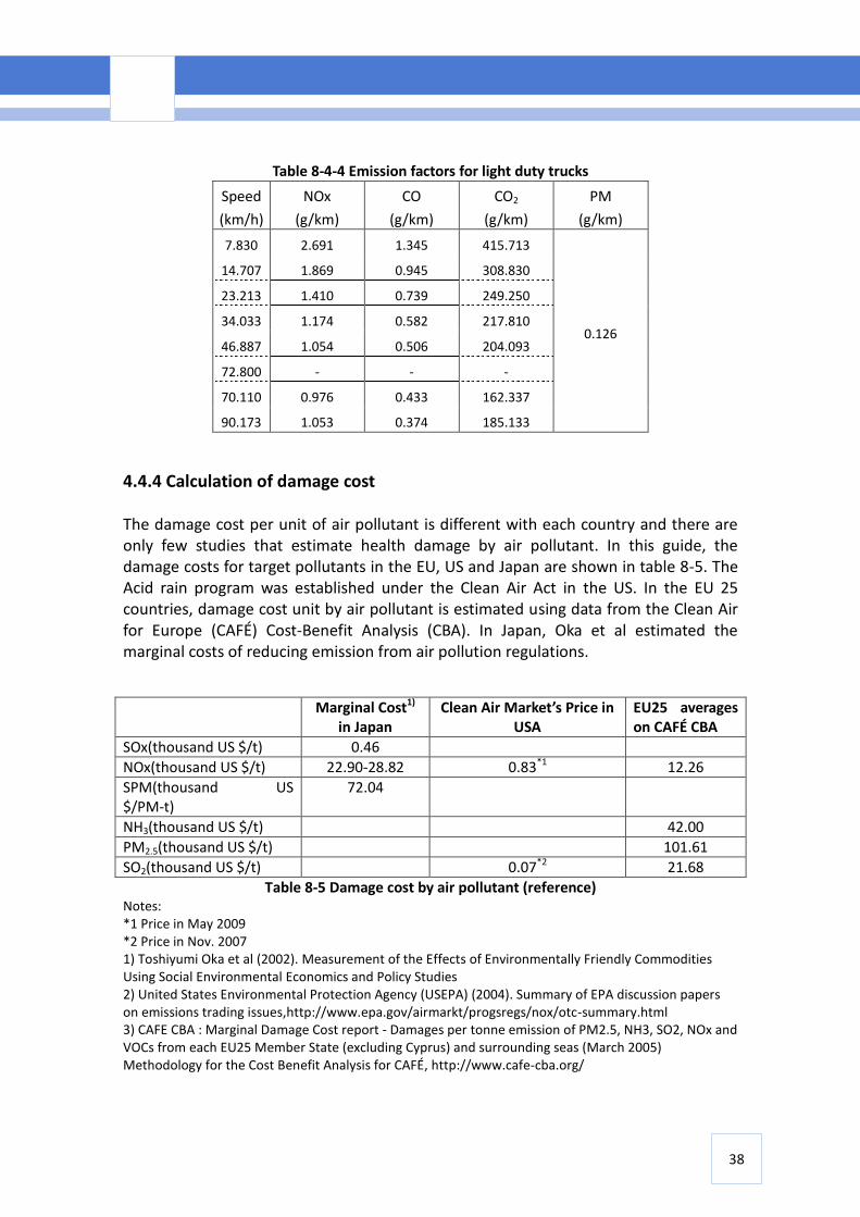
Table 8-4-4 Emission factors for light duty trucks

Speed

(km/h)

NOx

(g/km)

CO

(g/km)

CO2

(g/km)

PM

(g/km)

7.830 2.691 1.345 415.713

0.126

14.707 1.869 0.945 308.830

23.213 1.410 0.739 249.250

34.033 1.174 0.582 217.810

46.887 1.054 0.506 204.093

72.800 - - -

70.110 0.976 0.433 162.337

90.173 1.053 0.374 185.133

4.4.4 Calculation of damage cost The damage cost per unit of air pollutant is different with each country and there are only few studies that estimate health damage by air pollutant. In this guide, the damage costs for target pollutants in the EU, US and Japan are shown in table 8-5. The Acid rain program was established under the Clean Air Act in the US. In the EU 25 countries, damage cost unit by air pollutant is estimated using data from the Clean Air for Europe (CAFÉ) Cost-Benefit Analysis (CBA). In Japan, Oka et al estimated the marginal costs of reducing emission from air pollution regulations.

Table 8-5 Damage cost by air pollutant (reference) Notes: *1 Price in May 2009 *2 Price in Nov. 2007 1) Toshiyumi Oka et al (2002). Measurement of the Effects of Environmentally Friendly Commodities Using Social Environmental Economics and Policy Studies 2) United States Environmental Protection Agency (USEPA) (2004). Summary of EPA discussion papers on emissions trading issues,http://www.epa.gov/airmarkt/progsregs/nox/otc-summary.html 3) CAFE CBA : Marginal Damage Cost report - Damages per tonne emission of PM2.5, NH3, SO2, NOx and VOCs from each EU25 Member State (excluding Cyprus) and surrounding seas (March 2005) Methodology for the Cost Benefit Analysis for CAFÉ, http://www.cafe-cba.org/

Marginal Cost1)

in Japan Clean Air Market’s Price in

USA EU25 averages on CAFÉ CBA

SOx(thousand US $/t) 0.46

NOx(thousand US $/t) 22.90-28.82 0.83*1 12.26

SPM(thousand US $/PM-t)

72.04

NH3(thousand US $/t) 42.00

PM2.5(thousand US $/t) 101.61

SO2(thousand US $/t) 0.07*2 21.68

39

References Asian Development Bank (ADB) (2009). Transport and carbon dioxide emissions: forecasts, options, analysis, and evaluation, ADB, Manila, Philippines Ayres, R. and Walter, J. (1991). The greenhouse effect: damages, costs and abatement, Environmental and Resource Economics, 1 (3), 237-270. Bureau of Transport and Regional Economics Data (2003). Making travel safer: Victoria’s speed enforcement program., http://download.audit.vic.gov.au/reports_par/agp11602.html CAFE CBA, Marginal Damage Cost report - Damages per tonne emission of PM2.5, NH3, SO2, NOx and VOCs from each EU25 Member State (excluding Cyprus) and surrounding seas (March 2005) Methodology for the Cost Benefit Analysis for CAFÉ, http://www.cafe-cba.org/ Center for Clean Air Policy (CCAP) (2010) Transportation NAMAs: a proposed framework, hhttp://www.ccap.org/docs/resources/924/CCAP_Transport_NAMA.pdf Creutzig, F. and D. He (2009). Climate change mitigation and co-benefits of feasible transport demand policies in Beijing. Transport. Res. Part D 14(2), 120-131. den Boer, E. et al (2009). Are trucks taking their toll? The environmental, safety and congestion impacts of lorries in the EU. CE Delft, Netherlands. Intergovernmental Panel on Climate Change (IPCC) (Fourth Assessment Report). Climate Change, 2001: Mitigation. (2001)B. Metz, O. Davidson, R. Swart. and J. Pan. (eds.) Cambridge, Cambridge University Press. Japan Research Institute’s (JRI) (1999) ‘Guidelines for the Evaluation of Road Investment Projects.’ Leather, J. (2009). Rethinking Transport and Climate Change. Draft copy. Asian Development Bank. Manila, Philippines. Maibach, M. et al (2008). Handbook on estimation of external costs in the transport sector Version 1.1. CE Delft, Netherlands. Mohan, D. (2002). Social cost of road traffic crashes in India. Proceedings of First Safe Community Conference on Cost of Injury, Viborg, Denmark, pp. 33-38.

http://download.audit.vic.gov.au/reports_par/agp11602.html

http://www.cafe-cba.org/

40

Ministry of Land, Infrastructure and Tourism (MLIT) (2003). Study to promote CDM projects in the transport sector in order to resolve global environmental problems (Bangkok Metropolitan Area Case), Tokyo, Japan. Oka, T. (2002) Measurement of the Effects of Environmentally Friendly Commodities Using Social Environmental Economics and Policy Studies The Energy and Resources Institute (TERI) and World Business Council for Sustainable Development (2008). Mobility for Development: Bangalore, India. WBCSD, http://www.wbcsd.org/DocRoot/L6oFI1nA5XLSAqUb0aZU/M4D_Bangalore_case_study%20-%20small.pdf Uchida T. and Zusman, E. (2008). Reconciling local sustainable development benefits and global greenhouse gas mitigation in Asia: research trends and needs. Studies of Regional Policy 11(1), pp57-74 United Nations Framework Convention on Climate Change (UNFCCC) (2007). Bali Action Plan. http://unfccc.int/files/meetings/cop_13/application/pdf/cp_bali_action.pdf. UNFCCC (2009). Copenhagen Accord, http://unfccc.int/resource/docs/2009/cop15/eng/11a01.pdf. UNFCCC (2010). Cancun Agreements: Outcome of the work of the Ad Hoc Working Group on Long-term Cooperative Action under the Convention, http://unfccc.int/resource/docs/2010/cop16/eng/07a01.pdf#page=2 United States Environmental Protection Agency (USEPA) (2004). Summary of EPA discussion papers on emissions trading issues, http://www.epa.gov/airmarkt/progsregs/nox/otc-summary.html United States-Department of Transportation (US-DOT) Federal Highway Administration (2003). Enhanced night visibility Vol. XI, http://www.tfhrc.gov/safety/hsis/pubs/04142/benefit.htm Sanchez, S. (2008) Reforming CDM and scaling-up finance for sustainable urban transport in Olsen, K. H. and Fenhann, J. (eds) A Reformed CDM– Including New Mechanisms for Sustainable Development, UNEP Risø Centre, Roskilde, Denmark The World Bank, Global Purchasing Power Parities and Real Expenditures 2005 International Comparison Program

http://www.wbcsd.org/DocRoot/L6oFI1nA5XLSAqUb0aZU/M4D_Bangalore_case_study%20-%20small.pdf

http://www.wbcsd.org/DocRoot/L6oFI1nA5XLSAqUb0aZU/M4D_Bangalore_case_study%20-%20small.pdf

http://unfccc.int/resource/docs/2009/cop15/eng/11a01.pdf

http://www.tfhrc.gov/safety/hsis/pubs/04142/benefit.htm

41

CASE STUDIES

1. Proposed C-5 BRT (in Manila)

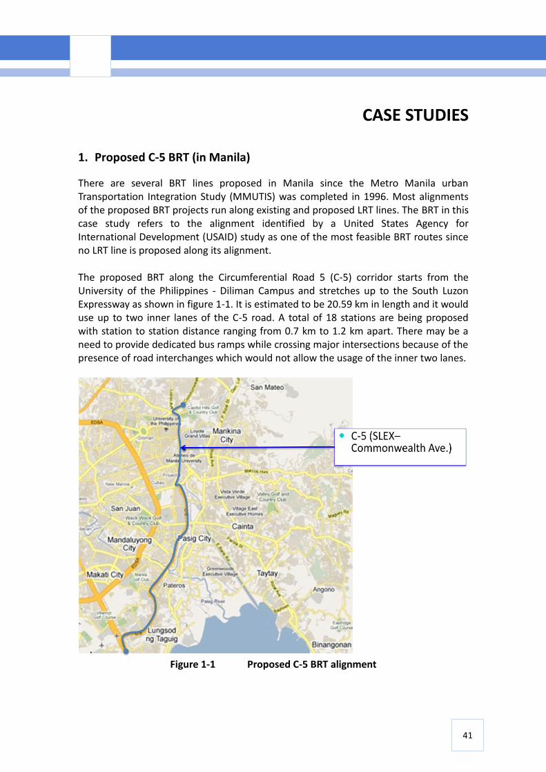
There are several BRT lines proposed in Manila since the Metro Manila urban Transportation Integration Study (MMUTIS) was completed in 1996. Most alignments of the proposed BRT projects run along existing and proposed LRT lines. The BRT in this case study refers to the alignment identified by a United States Agency for International Development (USAID) study as one of the most feasible BRT routes since no LRT line is proposed along its alignment. The proposed BRT along the Circumferential Road 5 (C-5) corridor starts from the University of the Philippines - Diliman Campus and stretches up to the South Luzon Expressway as shown in figure 1-1. It is estimated to be 20.59 km in length and it would use up to two inner lanes of the C-5 road. A total of 18 stations are being proposed with station to station distance ranging from 0.7 km to 1.2 km apart. There may be a need to provide dedicated bus ramps while crossing major intersections because of the presence of road interchanges which would not allow the usage of the inner two lanes.

Figure 1-1 Proposed C-5 BRT alignment

42

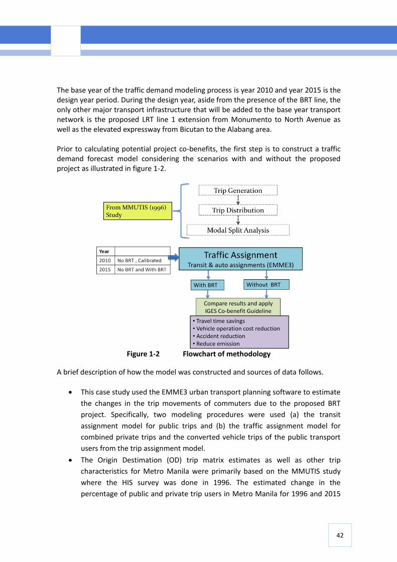
The base year of the traffic demand modeling process is year 2010 and year 2015 is the design year period. During the design year, aside from the presence of the BRT line, the only other major transport infrastructure that will be added to the base year transport network is the proposed LRT line 1 extension from Monumento to North Avenue as well as the elevated expressway from Bicutan to the Alabang area. Prior to calculating potential project co-benefits, the first step is to construct a traffic demand forecast model considering the scenarios with and without the proposed project as illustrated in figure 1-2.

Figure 1-2 Flowchart of methodology

A brief description of how the model was constructed and sources of data follows.

This case study used the EMME3 urban transport planning software to estimate

the changes in the trip movements of commuters due to the proposed BRT

project. Specifically, two modeling procedures were used (a) the transit

assignment model for public trips and (b) the traffic assignment model for

combined private trips and the converted vehicle trips of the public transport

users from the trip assignment model.

The Origin Destimation (OD) trip matrix estimates as well as other trip

characteristics for Metro Manila were primarily based on the MMUTIS study

where the HIS survey was done in 1996. The estimated change in the

percentage of public and private trip users in Metro Manila for 1996 and 2015

43

values were obtained from MMUTIS. Given the increasing trend in the use of

private modes, the total OD trip matrix estimates for year 2010 was

interpolated using the 1996 base year and 2015 design year percentage

estimates from MMUTIS. Hence for 2010, the multipliers are 0.693 to obtain

the OD matrix of public trips and 0.307 for private trips. For the year 2015, the

factor is 0.662 for public trips and 0.338 for private trips as obtained from the

MMUTIS study.

The trip generation growth estimates for Metro Manila as obtained from

MMUTIS for 2015 is 1.84% of the base year 1996. Assuming a linear growth

rate, the percent growth rate for year 2010 value was then interpolated, which

is 1.62.

In order to obtain the total daily OD trip matrix (sum of both public and private

trips) in Metro Manila for the year 2010, the total daily OD Matrix estimates of

the base year 1996 was simply multiplied by the factor of 1.62 for each OD pair.

For the year 2015, the factor is 1.84.

1.1 Traffic demand modeling

Snapshots of the traffic assignment results derived from the EMME3 model are shown in figures 1-3 and 1-4.

Figure 1-3 Estimated boarding and alighting along C-5 BRT stations

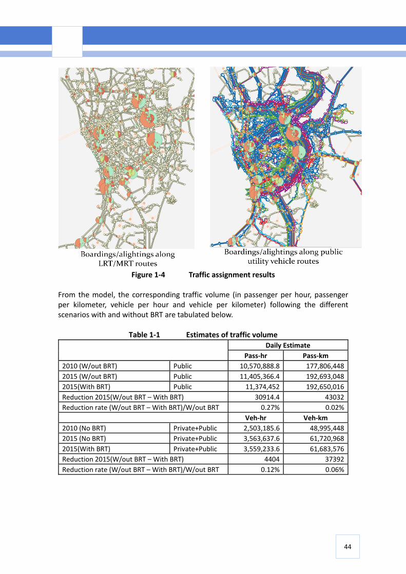
44

Figure 1-4 Traffic assignment results

From the model, the corresponding traffic volume (in passenger per hour, passenger per kilometer, vehicle per hour and vehicle per kilometer) following the different scenarios with and without BRT are tabulated below.

Table 1-1 Estimates of traffic volume

Daily Estimate

Pass-hr Pass-km

2010 (W/out BRT) Public 10,570,888.8 177,806,448

2015 (W/out BRT) Public 11,405,366.4 192,693,048

2015(With BRT) Public 11,374,452 192,650,016

Reduction 2015(W/out BRT – With BRT) 30914.4 43032

Reduction rate (W/out BRT – With BRT)/W/out BRT 0.27% 0.02%

Veh-hr Veh-km

2010 (No BRT) Private+Public 2,503,185.6 48,995,448

2015 (No BRT) Private+Public 3,563,637.6 61,720,968

2015(With BRT) Private+Public 3,559,233.6 61,683,576

Reduction 2015(W/out BRT – With BRT) 4404 37392

Reduction rate (W/out BRT – With BRT)/W/out BRT 0.12% 0.06%

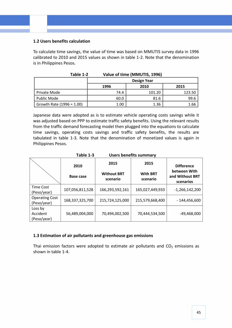
45

1.2 Users benefits calculation

To calculate time savings, the value of time was based on MMUTIS survey data in 1996 calibrated to 2010 and 2015 values as shown in table 1-2. Note that the denomination is in Philippines Pesos.

Table 1-2 Value of time (MMUTIS, 1996)

Design Year

1996 2010 2015

Private Mode 74.4 101.20 123.50

Public Mode 60.0 81.6 99.6

Growth Rate (1996 = 1.00) 1.00 1.36 1.66

Japanese data were adopted as is to estimate vehicle operating costs savings while it was adjusted based on PPP to estimate traffic safety benefits. Using the relevant results from the traffic demand forecasting model then plugged into the equations to calculate time savings, operating costs savings and traffic safety benefits, the results are tabulated in table 1-3. Note that the denomination of monetized values is again in Philippines Pesos.

Table 1-3 Users benefits summary

2010

Base case

2015

Without BRT scenario

2015

With BRT scenario

Difference

between With and Without BRT

scenarios

Time Cost (Peso/year)

107,056,811,528 166,293,592,161 165,027,449,933 -1,266,142,200

Operating Cost (Peso/year)

168,337,325,700 215,724,125,000 215,579,668,400 - 144,456,600

Loss by Accident (Peso/year)

56,489,004,000 70,494,002,500 70,444,534,500 -49,468,000

1.3 Estimation of air pollutants and greenhouse gas emissions

Thai emission factors were adopted to estimate air pollutants and CO2 emissions as shown in table 1-4.

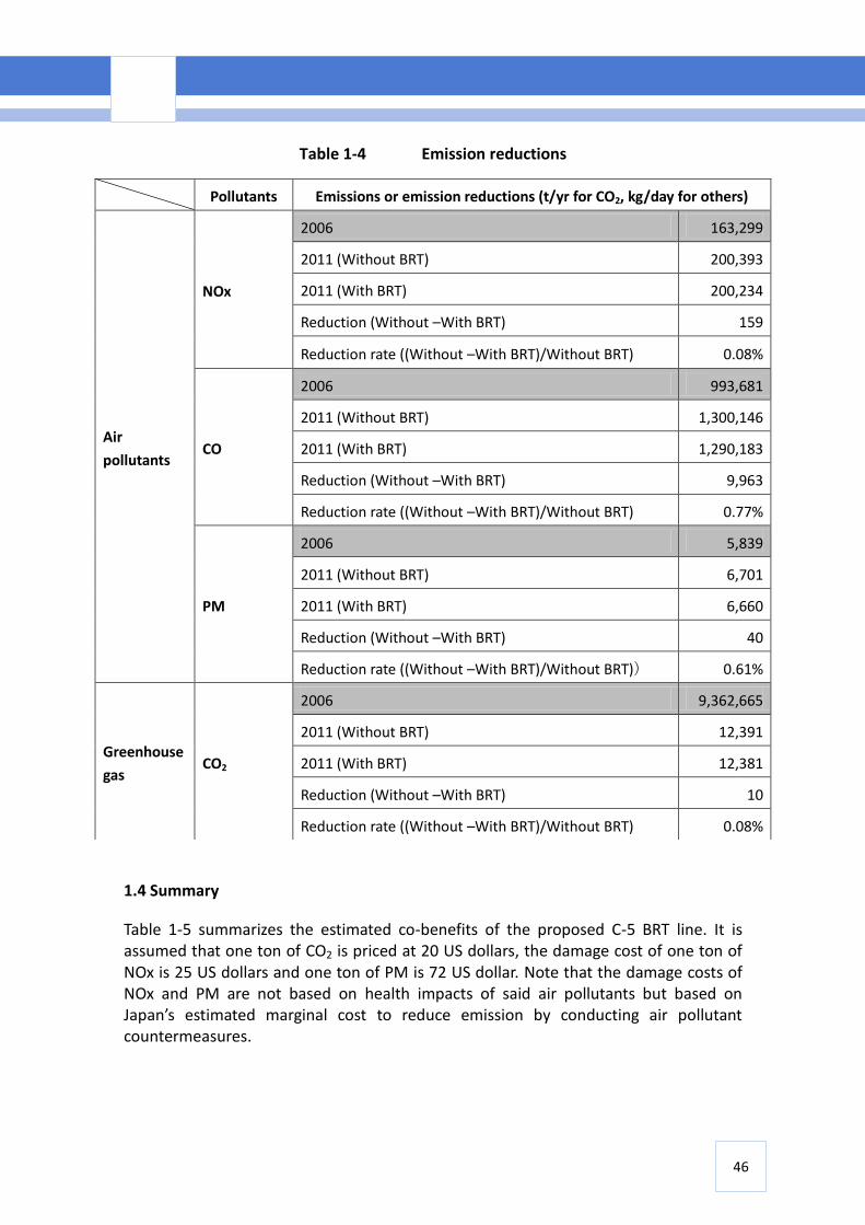
46

Table 1-4 Emission reductions

1.4 Summary

Table 1-5 summarizes the estimated co-benefits of the proposed C-5 BRT line. It is assumed that one ton of CO2 is priced at 20 US dollars, the damage cost of one ton of NOx is 25 US dollars and one ton of PM is 72 US dollar. Note that the damage costs of NOx and PM are not based on health impacts of said air pollutants but based on Japan’s estimated marginal cost to reduce emission by conducting air pollutant countermeasures.

Pollutants Emissions or emission reductions (t/yr for CO2, kg/day for others)

Air

pollutants

NOx

2006 163,299

2011 (Without BRT) 200,393

2011 (With BRT) 200,234

Reduction (Without –With BRT) 159

Reduction rate ((Without –With BRT)/Without BRT) 0.08%

CO

2006 993,681

2011 (Without BRT) 1,300,146

2011 (With BRT) 1,290,183

Reduction (Without –With BRT) 9,963


PM

2006 5,839

2011 (Without BRT) 6,701

2011 (With BRT) 6,660


Reduction rate ((Without –With BRT)/Without BRT)） 0.61%

Greenhouse

gas CO2

2006 9,362,665


2011 (With BRT) 12,381



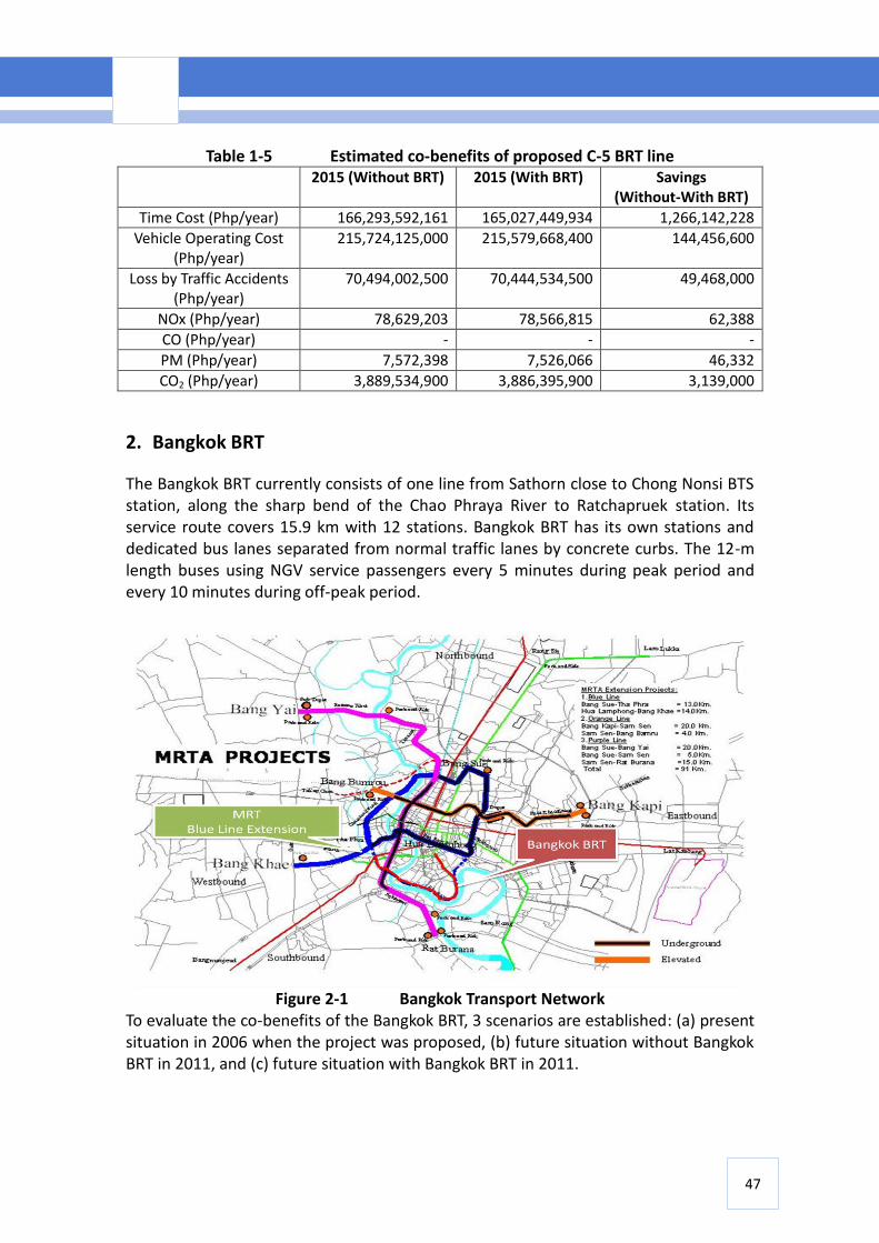
47

Table 1-5 Estimated co-benefits of proposed C-5 BRT line 2015 (Without BRT) 2015 (With BRT) Savings

(Without-With BRT)

Time Cost (Php/year) 166,293,592,161 165,027,449,934 1,266,142,228

Vehicle Operating Cost (Php/year)

215,724,125,000 215,579,668,400 144,456,600

Loss by Traffic Accidents (Php/year)

70,494,002,500 70,444,534,500 49,468,000

NOx (Php/year) 78,629,203 78,566,815 62,388

CO (Php/year) - - -

PM (Php/year) 7,572,398 7,526,066 46,332

CO2 (Php/year) 3,889,534,900 3,886,395,900 3,139,000

2. Bangkok BRT

The Bangkok BRT currently consists of one line from Sathorn close to Chong Nonsi BTS station, along the sharp bend of the Chao Phraya River to Ratchapruek station. Its service route covers 15.9 km with 12 stations. Bangkok BRT has its own stations and dedicated bus lanes separated from normal traffic lanes by concrete curbs. The 12-m length buses using NGV service passengers every 5 minutes during peak period and every 10 minutes during off-peak period.

Figure 2-1 Bangkok Transport Network

To evaluate the co-benefits of the Bangkok BRT, 3 scenarios are established: (a) present situation in 2006 when the project was proposed, (b) future situation without Bangkok BRT in 2011, and (c) future situation with Bangkok BRT in 2011.

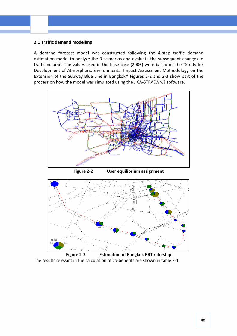
48

2.1 Traffic demand modelling

A demand forecast model was constructed following the 4-step traffic demand estimation model to analyze the 3 scenarios and evaluate the subsequent changes in traffic volume. The values used in the base case (2006) were based on the “Study for Development of Atmospheric Environmental Impact Assessment Methodology on the Extension of the Subway Blue Line in Bangkok.” Figures 2-2 and 2-3 show part of the process on how the model was simulated using the JICA-STRADA v.3 software.

Figure 2-2 User equilibrium assignment

Figure 2-3 Estimation of Bangkok BRT ridership

The results relevant in the calculation of co-benefits are shown in table 2-1.

乗換

乗車

降車

100人/日

凡例

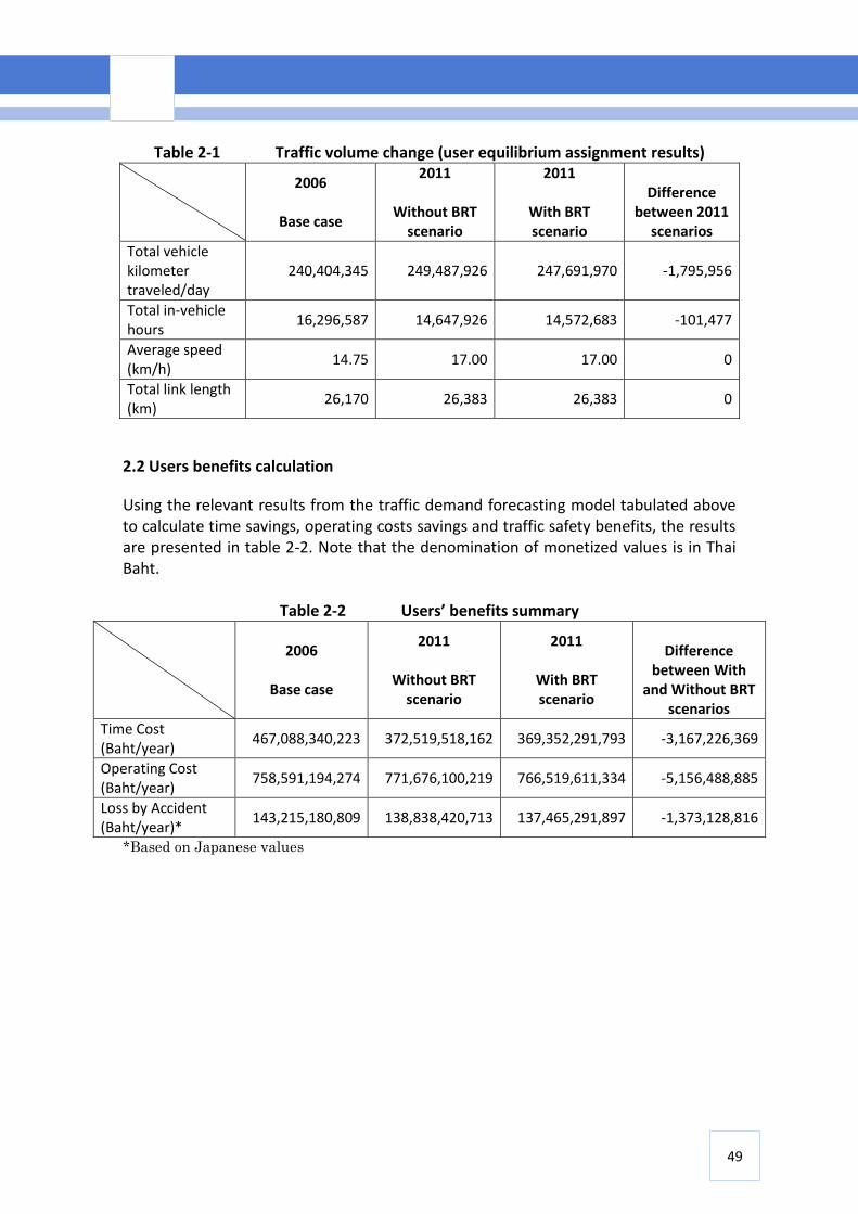
49

Table 2-1 Traffic volume change (user equilibrium assignment results)

2006

Base case

2011


2011

With BRT scenario

Difference

between 2011 scenarios

Total vehicle kilometer traveled/day

240,404,345 249,487,926 247,691,970 -1,795,956

Total in-vehicle hours

16,296,587 14,647,926 14,572,683 -101,477

Average speed (km/h)

14.75 17.00 17.00 0

Total link length (km)

26,170 26,383 26,383 0

2.2 Users benefits calculation

Using the relevant results from the traffic demand forecasting model tabulated above to calculate time savings, operating costs savings and traffic safety benefits, the results are presented in table 2-2. Note that the denomination of monetized values is in Thai Baht.

Table 2-2 Users’ benefits summary

2006

Base case

2011


2011

With BRT scenario

Difference

between With and Without BRT

scenarios

Time Cost (Baht/year)

467,088,340,223 372,519,518,162 369,352,291,793 -3,167,226,369

Operating Cost (Baht/year)

758,591,194,274 771,676,100,219 766,519,611,334 -5,156,488,885

Loss by Accident (Baht/year)*

143,215,180,809 138,838,420,713 137,465,291,897 -1,373,128,816

*Based on Japanese values

50

2.3 Estimation of air pollutants and greenhouse gas emissions

Air pollutants (NOx, PM, CO) and greenhouse gas (CO2) were estimated using the traffic volume and vehicle speed data for each link obtained through the 4-step traffic demand estimation model and applying the corresponding air pollutant emission factors. The results are summarized in table 2-3.

Table 2-3 Emission reductions

Pollutants Emissions or emission reductions (t/day for CO2, kg/day for others)

Air pollutants

NOx

2006

2011 (Without BRT) 327,389

2011 (With BRT) 325,930



CO

2006

2011 (Without BRT) 1,173,604

2011 (With BRT) 1,160,929


Reduction rate ((Without –With BRT)/Without BRT) 1.08

PM

2006


2011 (With BRT) 13,843



Greenhouse gas

CO2

2006


2011 (With BRT) 66,903



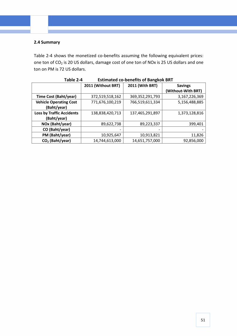
51

2.4 Summary

Table 2-4 shows the monetized co-benefits assuming the following equivalent prices:

one ton of CO2 is 20 US dollars, damage cost of one ton of NOx is 25 US dollars and one

ton on PM is 72 US dollars.

Table 2-4 Estimated co-benefits of Bangkok BRT 2011 (Without BRT) 2011 (With BRT) Savings

(Without-With BRT)

Time Cost (Baht/year) 372,519,518,162 369,352,291,793 3,167,226,369

Vehicle Operating Cost (Baht/year)

771,676,100,219 766,519,611,334 5,156,488,885

Loss by Traffic Accidents (Baht/year)

138,838,420,713 137,465,291,897 1,373,128,816

NOx (Baht/year) 89,622,738 89,223,337 399,401

CO (Baht/year) - - -

PM (Baht/year) 10,925,647 10,913,821 11,826

CO2 (Baht/year) 14,744,613,000 14,651,757,000 92,856,000

Institute for Global Environmental Strategies (IGES) 2108-11 Kamiyamaguchi, Hayama, Kanagawa, 240-0115 Japan TEL: +81-46-855-3700 FAX: +81-46-855-3709 E-mail: [email protected] URL: http://www.iges.or.jp [Tokyo Office] Nippon Press Center Bldg. 6F 2-2-1 Uchisaiwai-cho, Chiyoda-ku, Tokyo, 100-0011 Japan TEL: +81-3-3595-1081 FAX: +81-3-3595-1084 [Kansai Research Centre] East Building 4th Floor, Disaster Reduction and Human Renovation Institution, 1-5-2, Kaigan-dori, Waki-no-hama, Chuo-ku, Kobe, Hyogo, 651-0073 Japan TEL: +81-78-262-6634 FAX: +81-78-262-6635 [Kitakyushu Urban Centre] International Village Center 2F 1-1-1, Hirano, Yahata-Higashi-Ku, Kitakyushu City, JAPAN 805-0062 TEL: +81-93-681-1563 FAX: +81-93-681-1564 [Beijing Office] IGES Sino-Japan Cooperation Project Office Sino-Japan Friendship Center for Environmental Protection #508 Room No.1 Yuhuinanlu, Chao Yang District, Beijing, 100029 China TEL: +86-10-8463-6314 [Bangkok Office] c/o AIT/UNEP RRC.AP, Outreach Bldg. 3F, AIT P.O. Box 4, Klongluang, Pathumthani 12120, Thailand TEL: +66-2-524-6441 FAX: +66-2-516-2125 [APN Centre] East Building 4th Floor, Disaster Reduction and Human Renovation Institution, 1-5-2, Kaigan-dori, Waki-no-hama, Chuo-ku, Kobe, Hyogo, 651-0073 Japan TEL: +81-78-230-8017 FAX: +81-78-230-8018 [Japanese Center for International Studies in Ecology (JISE)] 2-12-20 Okano, Nishi-ku, Yokohama, Kanagawa, 220-0073 Japan TEL: +81-45-322-1223 FAX: +81-45-322-1225

mainstreaming transport co benefits approach co-benefits... · mainstreaming transport...

Documents