Magnetic Levitation

Bjørnar BøhagenDepartment of Engineering Cybernetics

Norwegian University of Science and TechnologyN-7491 Trondheim

NORWAY

2003

2

Contents

1 Introduction 5

2 Mathematical model 72.1 Mechanical model . . . . . . . . . . . . . . . . . . . . . . . . . . . 72.2 Electrical model . . . . . . . . . . . . . . . . . . . . . . . . . . . . 82.3 The overall model . . . . . . . . . . . . . . . . . . . . . . . . . . . 82.4 Stability . . . . . . . . . . . . . . . . . . . . . . . . . . . . . . . . 9

3 Control based on linear methods 113.1 Position control loop . . . . . . . . . . . . . . . . . . . . . . . . . 113.2 Current control loop . . . . . . . . . . . . . . . . . . . . . . . . . 123.3 The overall control loop . . . . . . . . . . . . . . . . . . . . . . . 13

4 Phase plane 15

5 The describing function method 17

6 Input-output linearization 196.1 Linearization . . . . . . . . . . . . . . . . . . . . . . . . . . . . . 196.2 Control . . . . . . . . . . . . . . . . . . . . . . . . . . . . . . . . 20

A The laboratory 23

3

4

1 Introduction

The magnetic levitation experiment, or for short "maglev", consists of an electro-magnet, a ball and a post encased in a rectangular enclosure as shown in Figure1. One electromagnet pole faces a black post upon which a 2.54 [cm] steel ball

Figure 1: The maglev experiment

rests. The ball elevation from the post is measured using a sensor embedded inthe post. The post is designed such that with the ball at rest on its surface, thetop of the ball is 12.5 [mm] from the face of the electromagnet (not 14 [mm] asstated in the manual [1]). The purpose of the experiment is to analyse and designcontrollers that levitates the ball from the post according to a desired set point ora desired trajectory. The post also provide repeatable initial condition for controlsystem performance evaluation. For further description and understanding of thesystem consult with [1] which is available in the laboratory.

5

6

2 Mathematical model

In this section we will derive a mathematical model for the system. First themechanical dynamics describing the ball is derived, then a model describing thecurrent in the electromagnet is derived. Before deriving the dynamics we definethe variables used in this section.

Definition 2.1

x1 = x

x2 = x

x3 = i

x =£x1 x2 x3

¤Tu = E

Be careful not to confuse the state vector, x, with the position variable, x. Inthe following all vectors will be expressed in bold face.

2.1 Mechanical model

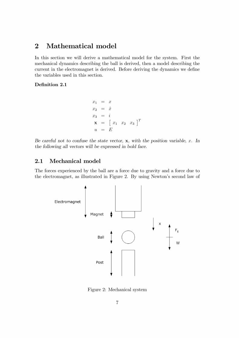
The forces experienced by the ball are a force due to gravity and a force due tothe electromagnet, as illustrated in Figure 2. By using Newton’s second law of

Figure 2: Mechanical system

7

motion, we may writemx =W − FE (1)

where m is the mass of the ball, x is the position at the top of the ball relativeto the electromagnet, W is the weight of the ball and FE is the force on the balldue to the electromagnet. The forces are given by

W = mg (2)

FE = Kii2

(x+ d)2(3)

where g is the acceleration due to gravity on the surface of the Earth, i is thecurrent running through the coil in the electromagnet, Ki is the magnetic forceconstant for the electromagnet/ball pair and d is a constant describing the "pointof attack" on the ball due to the electromagnetic force (notice that FE given hereis different from the one given in [1]). By using (2) and (3) we may rewrite (1) as

mx = W − FE

= mg −Kii2

(x+ d)2

⇔ x = g − Ki

m

i2

(x+ d)2(4)

2.2 Electrical model

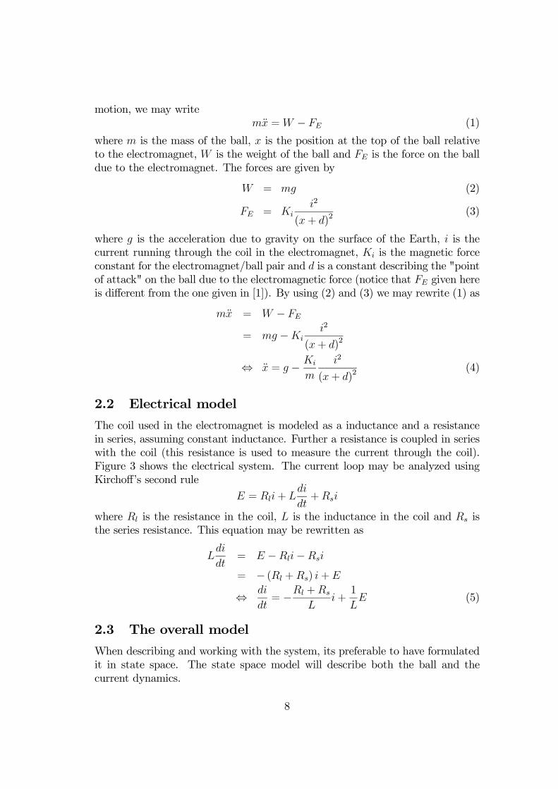
The coil used in the electromagnet is modeled as a inductance and a resistancein series, assuming constant inductance. Further a resistance is coupled in serieswith the coil (this resistance is used to measure the current through the coil).Figure 3 shows the electrical system. The current loop may be analyzed usingKirchoff’s second rule

E = Rli+ Ldi

dt+Rsi

where Rl is the resistance in the coil, L is the inductance in the coil and Rs isthe series resistance. This equation may be rewritten as

Ldi

dt= E −Rli−Rsi

= − (Rl +Rs) i+E

⇔ di

dt= −Rl +Rs

Li+

1

LE (5)

2.3 The overall model

When describing and working with the system, its preferable to have formulatedit in state space. The state space model will describe both the ball and thecurrent dynamics.

8

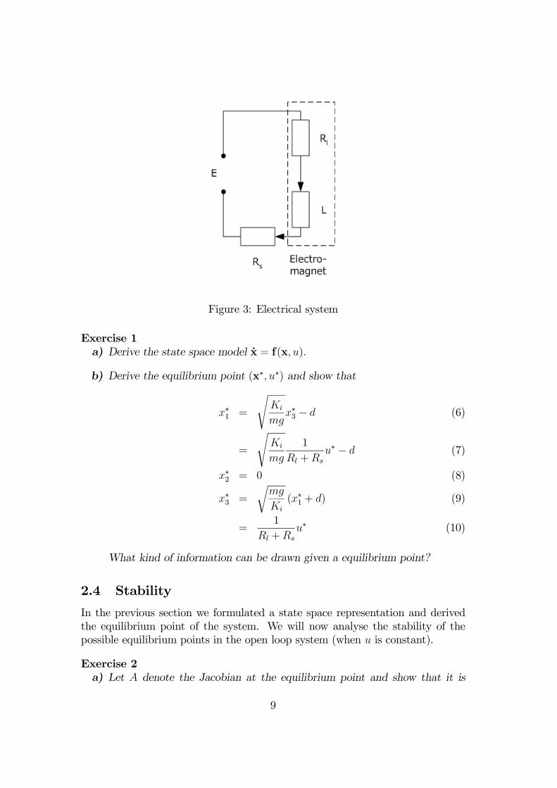
Figure 3: Electrical system

Exercise 1a) Derive the state space model x = f(x, u).

b) Derive the equilibrium point (x∗, u∗) and show that

x∗1 =

sKi

mgx∗3 − d (6)

=

sKi

mg

1

Rl +Rsu∗ − d (7)

x∗2 = 0 (8)

x∗3 =

rmg

Ki(x∗1 + d) (9)

=1

Rl +Rsu∗ (10)

What kind of information can be drawn given a equilibrium point?

2.4 Stability

In the previous section we formulated a state space representation and derivedthe equilibrium point of the system. We will now analyse the stability of thepossible equilibrium points in the open loop system (when u is constant).

Exercise 2a) Let A denote the Jacobian at the equilibrium point and show that it is

9

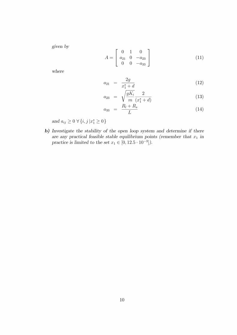
given by

A =

0 1 0a21 0 −a230 0 −a33

(11)

where

a21 =2g

x∗1 + d(12)

a23 =

rgKi

m

2

(x∗1 + d)(13)

a33 =Rl +Rs

L(14)

and aij ≥ 0 ∀ {i, j |x∗1 ≥ 0}b) Investigate the stability of the open loop system and determine if there

are any practical feasible stable equilibrium points (remember that x1 inpractice is limited to the set x1 ∈ [0, 12.5 · 10−3]).

10

3 Control based on linear methods

In [1] the distributor of the "maglev" experiment suggest a control law for thesystem based on linear theory. The closed loop system is designed in two stepsusing pole placement. First a control law for position (levitation) is designed,then a control law for the current loop is designed. When designing the positioncontrol loop, the current is used as control input assuming that the closed loopcurrent dynamics (the loop is closed with a control law) is infinite fast relativeto the position loop. In this section we will analyse this approach using theory,simulation and finally testing the control law on the actual system. First wedefine the variables used in this section.

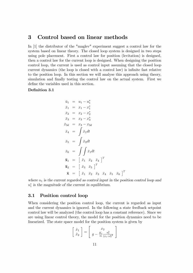
Definition 3.1

u1 = u1 − u∗1x1 = x1 − x∗1x2 = x2 − x∗2x3 = x3 − x∗3x3d = x3 − x3d

x4 =

Zx1dt

x5 =

Zx3dt

x6 =

Z Zx1dt

x1 =£x1 x2 x4

¤Tx2 =

£x3 x5

¤Tx =

£x1 x2 x3 x4 x5 x6

¤Twhere u1 is the current regarded as control input in the position control loop andu∗1 is the magnitude of the current in equilibrium.

3.1 Position control loop

When considering the position control loop, the current is regarded as inputand the current dynamics is ignored. In the following a state feedback setpointcontrol law will be analyzed (the control loop has a constant reference). Since weare using linear control theory, the model for the position dynamics need to belinearized. The state space model for the position system is given by·

x1x2

¸=

"x2

g − Ki

m

u21(x1+d)

2

#

11

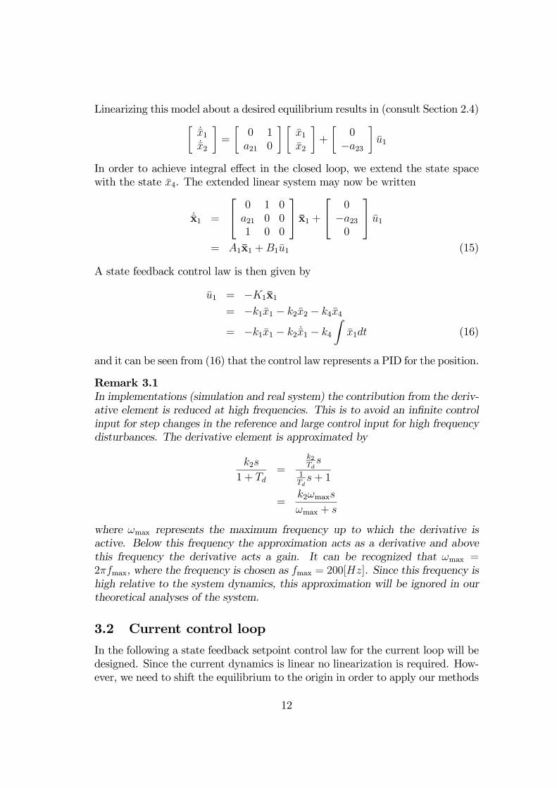
Linearizing this model about a desired equilibrium results in (consult Section 2.4)·˙x1˙x2

¸=

·0 1a21 0

¸ ·x1x2

¸+

·0−a23

¸u1

In order to achieve integral effect in the closed loop, we extend the state spacewith the state x4. The extended linear system may now be written

˙x1 =

0 1 0a21 0 01 0 0

x1 + 0−a230

u1= A1x1 +B1u1 (15)

A state feedback control law is then given by

u1 = −K1x1

= −k1x1 − k2x2 − k4x4

= −k1x1 − k2 ˙x1 − k4

Zx1dt (16)

and it can be seen from (16) that the control law represents a PID for the position.

Remark 3.1In implementations (simulation and real system) the contribution from the deriv-ative element is reduced at high frequencies. This is to avoid an infinite controlinput for step changes in the reference and large control input for high frequencydisturbances. The derivative element is approximated by

k2s

1 + Td=

k2Tds

1Tds+ 1

=k2ωmaxs

ωmax + s

where ωmax represents the maximum frequency up to which the derivative isactive. Below this frequency the approximation acts as a derivative and abovethis frequency the derivative acts a gain. It can be recognized that ωmax =2πfmax, where the frequency is chosen as fmax = 200[Hz]. Since this frequency ishigh relative to the system dynamics, this approximation will be ignored in ourtheoretical analyses of the system.

3.2 Current control loop

In the following a state feedback setpoint control law for the current loop will bedesigned. Since the current dynamics is linear no linearization is required. How-ever, we need to shift the equilibrium to the origin in order to apply our methods

12

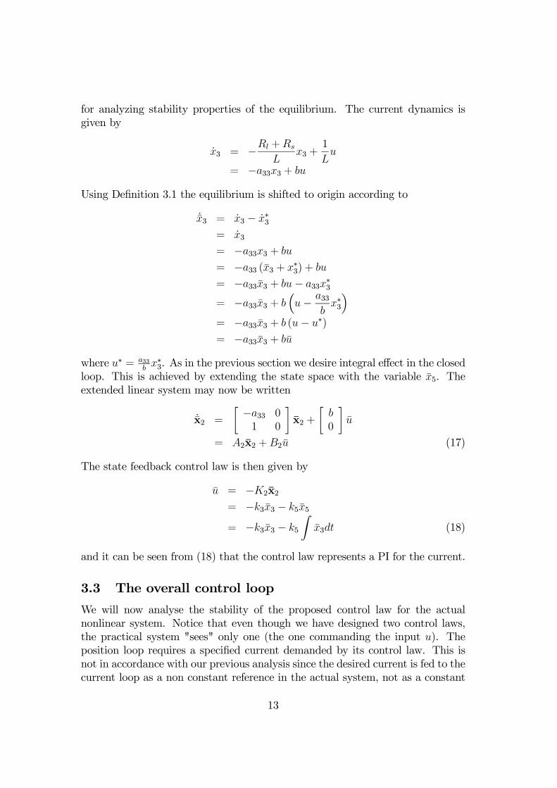
for analyzing stability properties of the equilibrium. The current dynamics isgiven by

x3 = −Rl +Rs

Lx3 +

1

Lu

= −a33x3 + bu

Using Definition 3.1 the equilibrium is shifted to origin according to

˙x3 = x3 − x∗3= x3

= −a33x3 + bu

= −a33 (x3 + x∗3) + bu

= −a33x3 + bu− a33x∗3

= −a33x3 + b³u− a33

bx∗3´

= −a33x3 + b (u− u∗)

= −a33x3 + bu

where u∗ = a33bx∗3. As in the previous section we desire integral effect in the closed

loop. This is achieved by extending the state space with the variable x5. Theextended linear system may now be written

˙x2 =

· −a33 01 0

¸x2 +

·b0

¸u

= A2x2 +B2u (17)

The state feedback control law is then given by

u = −K2x2

= −k3x3 − k5x5

= −k3x3 − k5

Zx3dt (18)

and it can be seen from (18) that the control law represents a PI for the current.

3.3 The overall control loop

We will now analyse the stability of the proposed control law for the actualnonlinear system. Notice that even though we have designed two control laws,the practical system "sees" only one (the one commanding the input u). Theposition loop requires a specified current demanded by its control law. This isnot in accordance with our previous analysis since the desired current is fed to thecurrent loop as a non constant reference in the actual system, not as a constant

13

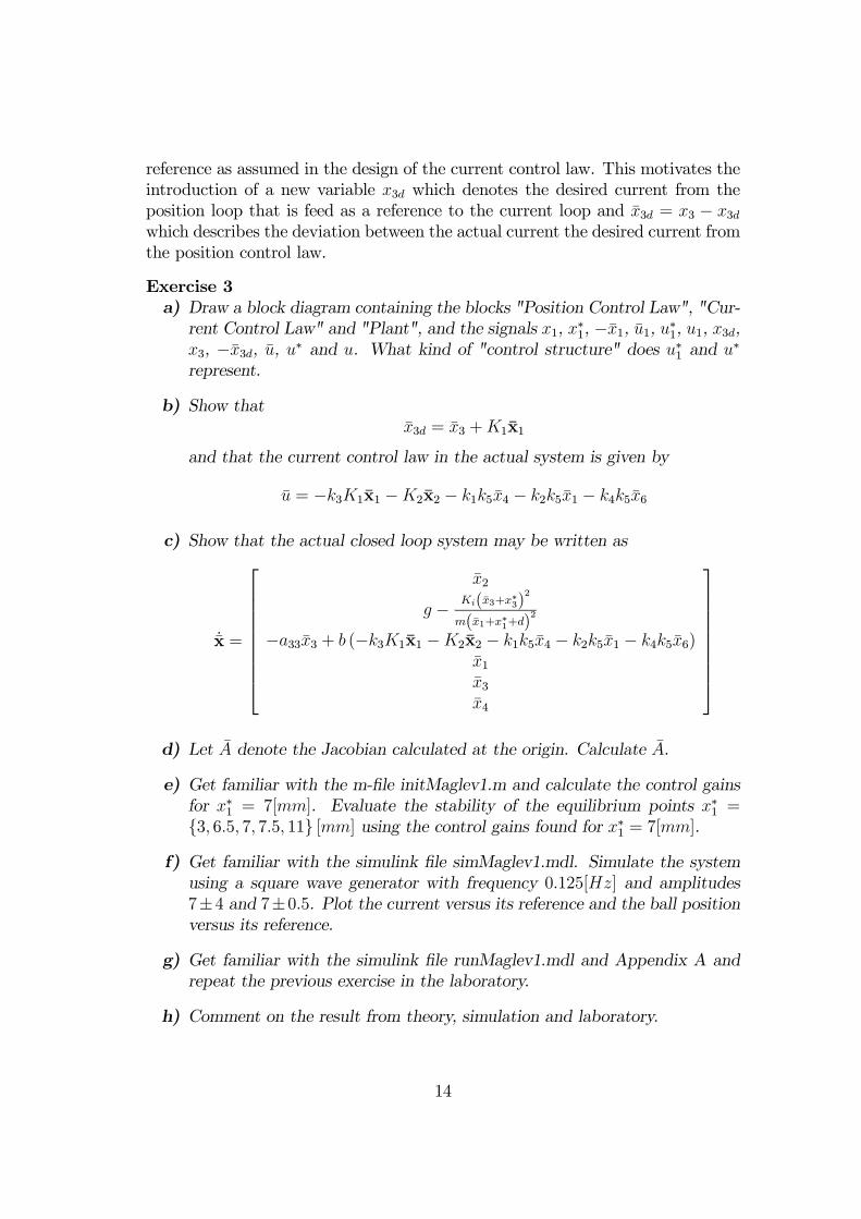
reference as assumed in the design of the current control law. This motivates theintroduction of a new variable x3d which denotes the desired current from theposition loop that is feed as a reference to the current loop and x3d = x3 − x3dwhich describes the deviation between the actual current the desired current fromthe position control law.

Exercise 3a) Draw a block diagram containing the blocks "Position Control Law", "Cur-rent Control Law" and "Plant", and the signals x1, x∗1, −x1, u1, u∗1, u1, x3d,x3, −x3d, u, u∗ and u. What kind of "control structure" does u∗1 and u∗

represent.

b) Show thatx3d = x3 +K1x1

and that the current control law in the actual system is given by

u = −k3K1x1 −K2x2 − k1k5x4 − k2k5x1 − k4k5x6

c) Show that the actual closed loop system may be written as

˙x =

x2

g − Ki(x3+x∗3)2

m(x1+x∗1+d)2

−a33x3 + b (−k3K1x1 −K2x2 − k1k5x4 − k2k5x1 − k4k5x6)x1x3x4

d) Let A denote the Jacobian calculated at the origin. Calculate A.

e) Get familiar with the m-file initMaglev1.m and calculate the control gainsfor x∗1 = 7[mm]. Evaluate the stability of the equilibrium points x∗1 ={3, 6.5, 7, 7.5, 11} [mm] using the control gains found for x∗1 = 7[mm].

f) Get familiar with the simulink file simMaglev1.mdl. Simulate the systemusing a square wave generator with frequency 0.125[Hz] and amplitudes7±4 and 7±0.5. Plot the current versus its reference and the ball positionversus its reference.

g) Get familiar with the simulink file runMaglev1.mdl and Appendix A andrepeat the previous exercise in the laboratory.

h) Comment on the result from theory, simulation and laboratory.

14

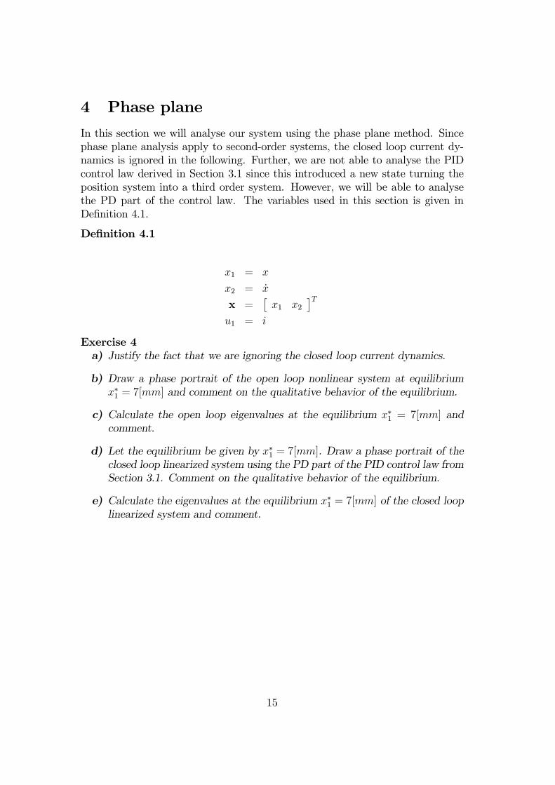
4 Phase plane

In this section we will analyse our system using the phase plane method. Sincephase plane analysis apply to second-order systems, the closed loop current dy-namics is ignored in the following. Further, we are not able to analyse the PIDcontrol law derived in Section 3.1 since this introduced a new state turning theposition system into a third order system. However, we will be able to analysethe PD part of the control law. The variables used in this section is given inDefinition 4.1.

Definition 4.1

x1 = x

x2 = x

x =£x1 x2

¤Tu1 = i

Exercise 4a) Justify the fact that we are ignoring the closed loop current dynamics.

b) Draw a phase portrait of the open loop nonlinear system at equilibriumx∗1 = 7[mm] and comment on the qualitative behavior of the equilibrium.

c) Calculate the open loop eigenvalues at the equilibrium x∗1 = 7[mm] andcomment.

d) Let the equilibrium be given by x∗1 = 7[mm]. Draw a phase portrait of theclosed loop linearized system using the PD part of the PID control law fromSection 3.1. Comment on the qualitative behavior of the equilibrium.

e) Calculate the eigenvalues at the equilibrium x∗1 = 7[mm] of the closed looplinearized system and comment.

15

16

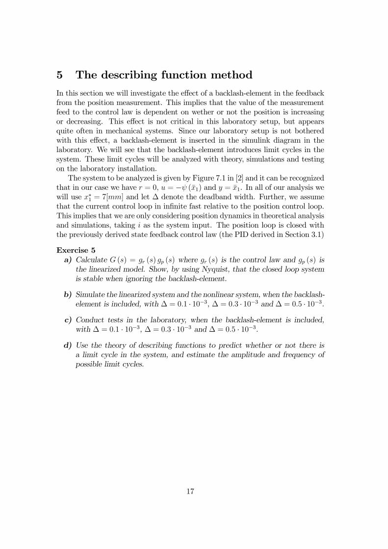
5 The describing function method

In this section we will investigate the effect of a backlash-element in the feedbackfrom the position measurement. This implies that the value of the measurementfeed to the control law is dependent on wether or not the position is increasingor decreasing. This effect is not critical in this laboratory setup, but appearsquite often in mechanical systems. Since our laboratory setup is not botheredwith this effect, a backlash-element is inserted in the simulink diagram in thelaboratory. We will see that the backlash-element introduces limit cycles in thesystem. These limit cycles will be analyzed with theory, simulations and testingon the laboratory installation.The system to be analyzed is given by Figure 7.1 in [2] and it can be recognized

that in our case we have r = 0, u = −ψ (x1) and y = x1. In all of our analysis wewill use x∗1 = 7[mm] and let ∆ denote the deadband width. Further, we assumethat the current control loop in infinite fast relative to the position control loop.This implies that we are only considering position dynamics in theoretical analysisand simulations, taking i as the system input. The position loop is closed withthe previously derived state feedback control law (the PID derived in Section 3.1)

Exercise 5a) Calculate G (s) = gr (s) gp (s) where gr (s) is the control law and gp (s) isthe linearized model. Show, by using Nyquist, that the closed loop systemis stable when ignoring the backlash-element.

b) Simulate the linearized system and the nonlinear system, when the backlash-element is included, with ∆ = 0.1 · 10−3, ∆ = 0.3 · 10−3 and ∆ = 0.5 · 10−3.

c) Conduct tests in the laboratory, when the backlash-element is included,with ∆ = 0.1 · 10−3, ∆ = 0.3 · 10−3 and ∆ = 0.5 · 10−3.

d) Use the theory of describing functions to predict whether or not there isa limit cycle in the system, and estimate the amplitude and frequency ofpossible limit cycles.

17

18

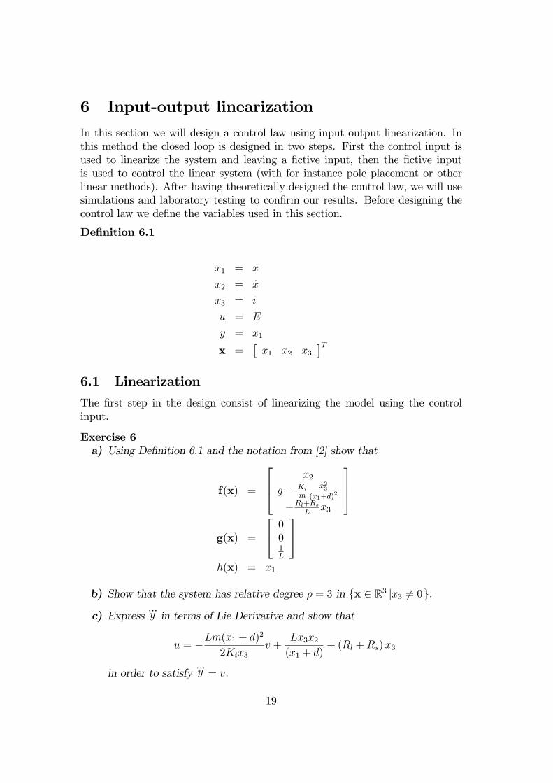
6 Input-output linearization

In this section we will design a control law using input output linearization. Inthis method the closed loop is designed in two steps. First the control input isused to linearize the system and leaving a fictive input, then the fictive inputis used to control the linear system (with for instance pole placement or otherlinear methods). After having theoretically designed the control law, we will usesimulations and laboratory testing to confirm our results. Before designing thecontrol law we define the variables used in this section.

Definition 6.1

x1 = x

x2 = x

x3 = i

u = E

y = x1

x =£x1 x2 x3

¤T6.1 Linearization

The first step in the design consist of linearizing the model using the controlinput.

Exercise 6a) Using Definition 6.1 and the notation from [2] show that

f(x) =

x2

g − Ki

m

x23(x1+d)

2

−Rl+Rs

Lx3

g(x) =

001L

h(x) = x1

b) Show that the system has relative degree ρ = 3 in {x ∈ R3 |x3 6= 0}.c) Express

...y in terms of Lie Derivative and show that

u = −Lm(x1 + d)2

2Kix3v +

Lx3x2(x1 + d)

+ (Rl +Rs)x3

in order to satisfy...y = v.

19

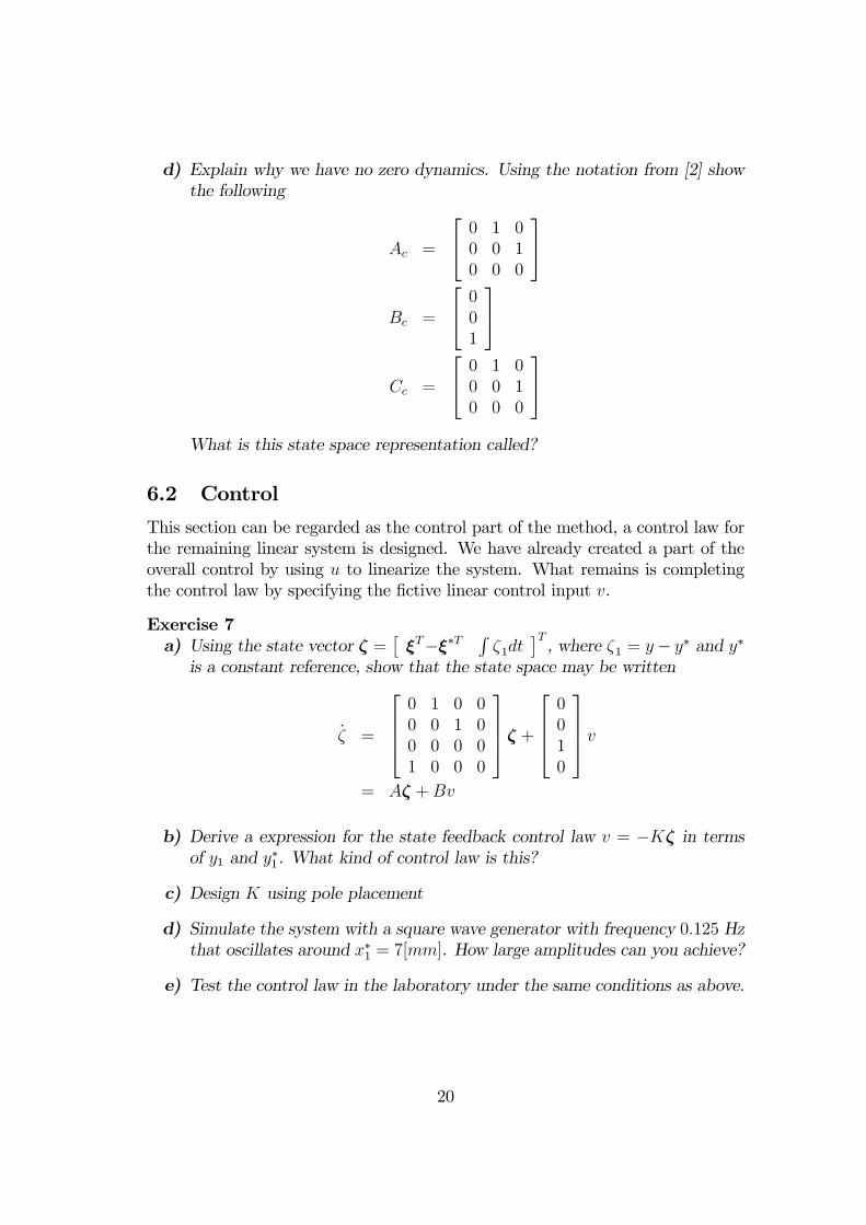
d) Explain why we have no zero dynamics. Using the notation from [2] showthe following

Ac =

0 1 00 0 10 0 0

Bc =

001

Cc =

0 1 00 0 10 0 0

What is this state space representation called?

6.2 Control

This section can be regarded as the control part of the method, a control law forthe remaining linear system is designed. We have already created a part of theoverall control by using u to linearize the system. What remains is completingthe control law by specifying the fictive linear control input v.

Exercise 7a) Using the state vector ζ =

£ξT−ξ∗T R

ζ1dt¤T, where ζ1 = y− y∗ and y∗

is a constant reference, show that the state space may be written

ζ =

0 1 0 00 0 1 00 0 0 01 0 0 0

ζ +0010

v= Aζ +Bv

b) Derive a expression for the state feedback control law v = −Kζ in termsof y1 and y∗1. What kind of control law is this?

c) Design K using pole placement

d) Simulate the system with a square wave generator with frequency 0.125 Hzthat oscillates around x∗1 = 7[mm]. How large amplitudes can you achieve?

e) Test the control law in the laboratory under the same conditions as above.

20

References

[1] Magnetic Levitation Experiment. Quanser Consulting. Advansed TeachingSystems.

[2] Khalil, Hassan K. Nonlinear Systems. Third Edition. Prentice Hall. 2002.

21