macroscopic traffic state estimation: understanding...
TRANSCRIPT
Research ArticleMacroscopic Traffic State Estimation Understanding TrafficSensing Data-Based Estimation Errors
Paul B C van Erp Victor L Knoop and Serge P Hoogendoorn
Department of Transport amp Planning Faculty of Civil Engineering and Geosciences Delft University of Technology Stevinweg 12628 CN Delft Netherlands
Correspondence should be addressed to Paul B C van Erp pbcvanerptudelftnl
Received 24 May 2017 Accepted 1 October 2017 Published 1 November 2017
Academic Editor Martin Trepanier
Copyright copy 2017 Paul B C van Erp et al This is an open access article distributed under the Creative Commons AttributionLicense which permits unrestricted use distribution and reproduction in any medium provided the original work is properlycited
Traffic state estimation is a crucial element in trafficmanagement systems and in providing traffic information to road users In thisarticle we evaluate traffic sensing data-based estimation error characteristics in macroscopic traffic state estimation We considertwo types of sensing data that is loop-detector data and probe speed data These data are used to estimate the mean speed in adiscrete space-timemeshWe assume that there are no errors in the sensing dataThis allows us to study the errors resulting from thedifferences in characteristics between the sensing data and desired estimate together with the incomplete description of the relationbetween the twoThe aimof the study is to evaluate the dependency of this estimation error on the traffic conditions and sensing datacharacteristics For this purpose we usemicroscopic traffic simulation wherewe compare the estimates with the ground truth usingEdiersquos definitions The study exposes a relation between the error distribution characteristics and traffic conditions Furthermorewe find that it is important to account for the correlation between individual probe data-based estimation errors Knowledge relatedto these estimation errors contributes to making better use of the available sensing data in traffic state estimation
1 Introduction
Traffic state estimation is an important element in trafficmanagement applications and traffic information servicesThe traffic state can be described on different levels [1] Themicroscopic traffic state describes the traffic on an individ-ual vehicle level thus using the time and space headwaysand individual vehicle speed The macroscopic traffic statedescribes the traffic flow conditions using the mean speeddensity and flow
In traffic state estimation different types of informationcan be used Traffic sensing data is collected via differentkind of sensors for example loop-detectors [2 3] andmobile phones (probes) [4 5] In addition to sensing datainformation related to the traffic dynamics is captured in theform of traffic flow models for example the LWR model[6 7] Traffic flow models are based on physical laws andhistorical data These information types thus sensing dataand traffic flow models allow us to estimate the traffic stateThe difference between the true and estimated traffic states is
denoted as the estimation error In this research the focus isput on these estimation errors
It is valuable to have information related to the estimationerrors for applications of the related estimates For instancein traffic state estimation different types of informationfor example traffic sensing data-based estimates and trafficflow model-based prediction can be fused Examples ofsuch applications are [3ndash5 8] These applications all consider(amongst others) a variant of the Kalman Filter (KF) [9]for information fusion KFs assume Gaussian distributederrors with a to-be-defined (co)variance Alternatively aParticle Filter (PF) [10] can be used for information fusionin which we are free to define any type of expected errordistribution In the provided references related to the KFthe researchers all assume constant error variances relatedto the data-based that is loop-detector or probe data-based estimates They thus do not assume any dependencyof the error characteristics on features such as the trafficconditions or varying sensing data characteristics In additionto information fusion information related to estimation or
HindawiJournal of Advanced TransportationVolume 2017 Article ID 5730648 11 pageshttpsdoiorg10115520175730648
2 Journal of Advanced Transportation
prediction errors can also have a more direct value for roadusers For instance in travel time prediction a probabilityfunction can be provided instead of a single expected value[11] This may be valuable for routing advise as the traveltime variability may negatively influence the attractiveness ofcertain routes
In this research the following way of thinking is consid-ered If we have knowledge related to the relation betweenestimation error characteristics and potentially observablefeatures we may improve our understanding of the errorcharacteristics related to an estimate Examples of potentiallyobservable features are traffic conditions and sensing datacharacteristics Improved understanding of the estimationerror characteristics is valuable in the applications discussedabove for example traffic state estimation using a variant ofthe KL [3 4 8]
The objective of this research is to expose the dependencyof traffic sensing data-based estimation errors on trafficconditions and sensing data characteristics We define trafficsensing data-based estimation as the estimation of a desiredoutput based on traffic sensing data Both the sensing data asthe desired output have specific characteristics for exampletype of variable and spatialtemporal characteristics If thesediffer we have to make assumptions to describe the relationbetween the two In this research we estimate the meanspeed in discrete time and space that is time is discretizedin periods and space in cells (road segments) similar to[3 4 8 12 13] The properties of the traffic sensing data-typewe consider that is loop-detector data and probe speed dataare based on existing research [4 14]
This research focuses on specific combinations of trafficsensing data and estimation output The findings can beused for applications which consider similar data-types andestimation output However more generally we opt to showthat the estimation error characteristics can depend on thetraffic conditions and (varying) sensing data characteristicsAny application that requires defining the estimation errorcharacteristics for example information fusion using a KFcan take this into account However depending on thespecific application this may require extra research
In this article we first describe the (macroscopic) trafficconditions within a discrete space-time mesh Next wediscuss traffic sensing data-based traffic state estimation andour focus related to this topic After describing the conductedexperiments we present and discuss the results Finally theconclusions of this research are presented
2 Variables Used to Describethe Traffic Conditions
The traffic conditions can be described as a function of space119909 and time 119905 For computational reasons it is valuable toconsider the traffic conditions in discretized space and time[15] To discretize the space 119909 the road stretch is subdividedinto 119868 cells where 119894 and Δ 119894 respectively denote the cellnumber and length of cell 119894 The number of lanes within 119894 isgiven by 120582119894 Furthermore time 119905 is discretized in time periodswith duration 119879 which are denoted by 119901 = 1 119875 Eachcombination of 119894 and 119901 corresponds to a discrete area in
the space-time domain In this discrete space-time mesh themacroscopic traffic variables mean speed flow and densityare respectively denoted by 119906(119894 119901) 119902(119894 119901) and 120588(119894 119901)
In the literature different methodologies are proposedto calculate the macroscopic variables in a discrete space-time mesh based on the microscopic variables For instanceWang and Papageorgiou [3] propose calculating each variableindependently based on the downstream (flow) and end-of-period (mean speed and density) conditions AlternativelyEdie [16] proposed a generalized formulation of the macro-scopic variables In this research we followEdiersquos formulationas it considers the conditions over the entire space-time areainstead of only the end-of-period and downstream boundaryconditions
In traffic state estimation in a discrete space-time meshhomogeneous conditions (defined as constant over space)and stationary conditions (defined as constant over time) areoften assumed [8] Different vehicle classes (eg passengercars and trucks) can coexist in homogeneous and stationaryconditions namely if the conditions within these classes arehomogeneous and stationary
Assumptions related to homogeneity and stationaritycan be important when applying a traffic flow modelFor instance the Cell Transmission Model (CTM) [12 13]assumes a constant cell outflow during the entire period 119901 Itis however also important in sensing data-based estimationIn nonhomogeneous conditions a loop-detector placed atthe upstream cell boundary may observe different trafficconditions than one placed at the downstream boundaryIf the conditions are homogeneous both loop-detectorsobserve the same conditions and a loop-detector placed at anylocation within the cell is representative for the conditionsin the entire cell Furthermore the variation in individualvehicle speeds V can increase when the traffic conditions arenonhomogeneous and nonstationaryThis can lead to a largerestimation uncertainty when estimating the traffic conditionsbased on individual probe speeds
In reality traffic is nonhomogeneous and nonstationary[17] Such traffic conditions can still be expressed in themacroscopic traffic flow variables but these variables may beincapable of uniquely describing the traffic conditions Forinstance in terms of the (traditional) macroscopic variablesan area in which vehicles are decelerating due to downstreamcongestion (jam inflow) and in which vehicles are accelerat-ing when leaving a jam may be the same while in reality theconditions differ
To capture the conditions that are nonhomogeneous ornonstationary extra traffic variables can be used In thisresearch we add a single extra traffic variable related to thenonhomogeneity of traffic that is the change in speed overspace Although it is possible to add more variables addingthis single variable suffices for the analysis conducted in ourexperiments
3 Sensing Data-Based Mean Speed Estimation
Theexplanation of sensing data-basedmean speed estimationis split into three parts First we discuss the traffic sensingdata considered in this research Second the estimation
Journal of Advanced Transportation 3
approach to obtain the mean speed from the sensing datais presented And third we discuss how the estimation errordistribution can be described
31 Traffic Sensing Data Characteristics Seo [18] states thatwe can regard traffic data collection as a special case of trafficstate estimation In the procedure to obtain traffic data fromraw sensor signals exogenous assumptions are required Inthis research the starting point is traffic sensing data Weassume that these data do not contain errorsThis assumptionallows us to study the errors induced due to differencesbetween the sensing data characteristics and desired estimatecharacteristics and incomplete description of the relationbetween the two
We consider two types of traffic sensing data that is loop-detector data and probe speed data The characteristics ofthe loop-detector data are based on the loop-detector dataavailable in Netherlands that is lane-specific one-minuteaggregated (time-mean) speeds 119906119879119897 and flows 119902119897 [14] Fol-lowing [3] the loop-detectors are located at the downstreamboundary of discrete road segments In line with [4 5] weconsider instantaneous individual vehicle speeds from probevehicles that is V119899 where 119899 describes the vehiclersquos ID It isassumed that the probes are observed at the end of eachperiodThese data can be collected fromGPS-enabledmobilephones and navigation systems
32 Estimation Approach The desired estimation outputhas specific characteristics that is variable type and spa-tialtemporal characteristics In this research we estimate themean speed 119906 for a cell (discrete road segment) 119894 and period119901 that is 119906(119894 119901) This desired output is estimated based onthe two traffic sensing data-types discussed above
The traffic sensing data (partly) and desired output differin terms of variable type and spatialtemporal characteristicsTherefore we have to define models to estimate 119906(119894 119901) basedon the sensing data The models used in this research aretaken from prior research that is [4 14]
The loop-detector data and probe speed data-based esti-mates are respectively denoted as ld and probe Based onthe loop-detector data the speed is estimated by taking theweighted harmonic mean of the lane-specific speeds [14]Here we consider the loop-detector data which relates to thecell and period for which 119906 is estimated
ld = sum120582119897=1 119902119897sum120582119897=1 (119902119897119906119879119897 ) (1)
We consider themean V119899 of the 119895number of vehicles observedin a specific cell and period as the probe data-based 119906estimate that is probe [4]
probe = 1119895119895sum119899=1
V119899 (2)
33 Estimation Error Distribution The traffic sensing data-based estimates may differ from the true 119906(119894 119901) We denotethis difference as the sensing data-based estimation errorThe
characteristics of these errors may be described using theerror distribution
We describe the estimation error distribution using fourstatistics namely themean variance skewness and kurtosisThe mean variance skewness and kurtosis respectivelyrelate to the first second third and fourth standardizedmoments of a distribution [19] The skewness addressesthe symmetry of a distribution and the kurtosis providesinformation related to the peakedness or alternatively the ldquofattailsrdquo of a distribution [19] For perfect Gaussian distributionthe skewness and kurtosis are respectively equal to 0 and 3By means of the Jarque-Bera (JB) test [20] we can test fornormality The null hypothesis of the JB test is normality
4 Experimental Set-Up
The objective of the experiments is to expose the character-istics of the data-based mean speed estimation errors In thissection we discuss the data used in this research and explainthe conducted experiments
41 DataCollection In this research we consider synthesizeddata collected using the microscopic simulation programFOSIM The microscopic models and calibration used inFOSIM are described in [21] Furthermore it is validatedfor Dutch freeways [22 23] FOSIM allows us to retrievetrajectory data for each individual vehicle The trajectorydata are used for two purposes Firstly we construct thetraffic sensing data that is loop-detector data and probespeed data with the characteristics described in the previoussection Secondly we construct the ground truth as will beexplained below Combined these allow us to obtain thetraffic sensing data-based estimation errors and evaluate theircharacteristics
Real trajectory datasets are scarce and are often limitedin terms of spatial and temporal coverage For instancethe NGSIM [24] trajectory dataset covers a study area ofapproximately 640m for a 45-minute period FOSIM allowsus to simulate traffic for a much larger spatial and temporalcoverage
We consider a schematized road stretch of the Dutch A13freeway from the Hague to Rotterdam which has a speedlimit of 100 kmh in our experiments The length of the roadstretch is 13878m with five on-ramps and four off-rampsThe road is discretized in 24 cells with lengths ranging from520 to 770m We consider a two-hour time domain which isdiscretized into periods of 15 seconds 119879 = 153600 h Thisdiscretization is based on the approach followed by [3] Theroad layout and the traffic conditions in terms of 119906 and 120588are shown in Figure 1 Within this space-time domain twostanding queues are observed
42 Ground Truth Theground truth is important to describethe true traffic conditions in a discrete area in the space-timedomain and determine the estimation errors by comparingthe data-based estimates with the ground truth As explainedbefore we describe the macroscopic traffic conditions byfour variables namely the mean speed density flow and
4 Journal of Advanced Transportation
5
3
12
4
(a) Road layout in FOSIM
Time (h)
Spac
e (km
)
0
2
4
6
8
10
12
10
20
30
40
50
60
70
80
90
100
02 04 06 08 12 14 16 181 2
(b) Mean speed 119906 kmh
Time (h)
Spac
e (km
)0
2
4
6
8
10
12
50
100
150
200
02 04 06 08 12 14 16 181 2
(c) Density 120588 vehkm
Figure 1The schematized road stretch in FOSIM (a) and the true traffic conditions ((b) and (c)) in terms of the mean speed 119906 and density 120588
change in speed over space The former three variables aredetermined using [16] generalized formulation
120588 = sum119899 119903119899Δ119879 119902 = sum119899 119889119899Δ119879 119906 = 119902120588
(3)
where the time spent and distance traveled by vehicle 119899withinthe space-time area are respectively denoted by 119903119899 and 119889119899
The change in speed over space is obtained by performingan OLS regression over the end-of-period individual vehiclespeeds For this purpose we consider the following equationV119899 = 1205790 + 1205791119909119899 The change in speed over space is captured in1205791
Given the ground truth 119906 and data-based estimate theestimation error 120578 can be determined
120578 = 119906 minus (4)
43 Evaluation of Estimation Error Characteristics In thisresearch we evaluate the dependency of loop-detector andprobe data-based estimation error distributions on the trafficconditions Here the probe data-based estimates are basedon individual probe observations In reality we may havemultiple probe observations for a given combination of celland period Therefore we will also consider the dependency
of the probe data-based estimation error characteristicson the observed fraction of the traffic flow This sensingdataset characteristic is denoted by the number of probeobservations
431 Dependency on Traffic Conditions The traffic condi-tions can be described using the traffic flow variables Theestimation errors may be directly explained based on thetraffic flow variables using for instance linear regressionProblems with this approach are that the explanatory vari-ables are correlated (as described by fundamental diagramseg [25]) and nonlinear relations may exist between theexplanatory and dependent variables Instead of consideringthe traffic flow variables as independent variables we wantto identify the different traffic conditions in the considereddataset based on the combination of these variables Forthis purpose the true traffic conditions are grouped into adiscrete number of clusters using the 119870-means clusteringalgorithm Next the estimation error characteristics of theobservations assigned to each cluster can be described Thisapproach allows us to get an insight into the dependency ofthe estimation errors on the traffic conditions
Using the 119870-means clustering algorithm [26] each areain time and space is assigned to one of the defined119870 numberof clusters based on the traffic conditions These conditionsare described by three variables namely the mean speed119906 density 120588 and change in individual vehicle speeds overspace 120597V120597119909 The vector 119911(119900) contains these three variables
Journal of Advanced Transportation 5
for observation 119900 where 119900 relates to a single area in space-time domain The macroscopic traffic variable flow 119902 is leftout because 119906 and 120588 combined contain this information thatis 119902 = 120588119906 and in contrast to 119902 are able to uniquely describethe homogeneous and stationary traffic conditions119870-Means clustering follows an iterative procedure tominimize a cost function 119869cost This iterative procedure issusceptible to local optimaThismeans that the algorithm canconverge to different solutions To overcome this problem thealgorithm is applied 10 times and the solution with the lowestcost 119869cost is selected
We consider the cost function given by (5) This functionconsiders the mean squared difference between the individ-ual observations 119911(119900) and centroid of the assigned cluster 120583119888(119900)for the total number of observations 119898 Here the clustercentroid 120583119888(119900) is defined as the mean values for each variableof all observations assigned to cluster 119888
119869cost = 1119898119898sum119900=1
10038171003817100381710038171003817119911(o) minus 120583119888(119900)100381710038171003817100381710038172 (5)
Before applying the clustering algorithm the explanatoryvariables (features) are scaled If feature scaling is not appliedit is possible that features with larger absolute difference willdominate the clustering Therefore for each feature the 119911-scores are considered The 119911-score of an observation is equalto the difference between the observation and the meanof all observations divided by the standard deviation of allobservations
To find the optimal 119870 we plot 119869cost as a function of 119870Increasing 119870 will decrease the cost since a more refinedclustering is possible However this plot allows us to visuallycompare benefits in terms of 119869cost of addingmore clustersTheoptimal119870 is selected by searching for a kink which is referredto as the elbow in the plot Up till this point adding a clusteryields a relatively large benefit and thus a decrease in 119869costwhile the added value of increasing the number of clusters islimited Therefore the selected number of clusters is at thelocation of the elbow This selection procedure is subjectiveas we have to define what is a kink and what is notThereforeit is also important to interpret the cluster characteristics andsee if they make sense As will be shown in the results theselection procedure works well in our application
After each observation has been assigned to a clus-ter the estimation error distribution characteristics can bedetermined per cluster We are specifically interested in thedifferences between clusters Here the cluster characteristicsas described by the cluster centroids can be compared withthe error characteristics as described by the error statistics
We assume that the loop-detectors are located at thedownstream boundary of each road segment Based on thesedata a single 119906 estimate is obtained for each combination of119894 and 119901 119894 119901 Furthermore in this part of the research weconsider every possible individual probe data-based speedestimateThe number of vehicles on road segment 119894 in period119901 is defined as 119873(119894 119901) Therefore for each combinationof 119894 119901 one loop-detector and 119873(119894 119901) probe data-basedestimates are obtained
432 Dependency on Observed Fraction of the Traffic FlowThe probe data-based estimate (see (2)) and thus the probedata-based estimation error depend on the number of probeobservations 119895 We are interested in the effect of 119895 on estima-tion error characteristics Here we focus on the estimationerror variance as this is an important feature in trafficstate estimation methodologies which apply a KF and werediscussed in Introduction that is [3ndash5 8]
Models to Explain Probe Data-Based Estimation Error Vari-ance Wewill compare twomodels that describe the influenceof the number of probe observations 119895 on the estimation errorvariance The difference between these models relates to theexpected correlation between estimation errors of individualprobe observations
The first model assumes that individual probe data-basedestimates have the same error variance and the estimationerrors are not correlated In contrast the second model doesassume that there is a correlation between the individualestimation errors The rationale behind the second model isas follows The mean speed is dependent on the speeds ofall vehicles within the considered area in space-time In thiscase the difference between an individual vehicle speed V119899of vehicle 119899 and the mean speed 119906 that is the estimationerror is expected to be correlated with the difference betweenV119898 and 119906 that is the estimation error based on V of vehicle119898 For example if we have two observations the differencewith respect to the mean (error) of the two observations hasa correlation of minus one
The assumptions discussed above are used to analyticallyderive the two models For both models it is assumedthat V are Gaussian-distributed with mean 119906 and variance1205902V Given this distribution we can say that the estimationerror distribution based on single probe observations isa zero-mean Gaussian distribution with variance 1205902V Thisvariance is constant for a given area in the space-timedomain but can differ between areas for example due totraffic conditions In the first model each observation isseen as an independent observation with no relation to otherobservations thus 119864[120576119899120576119898] = 0 for 119899 = 119898 where 120576119899 denotesthe difference between 119906 and V119899 that is the estimationerror when estimating 119906 based on the individual speed V ofvehicle 119899 In the second model we take into account the factthat the estimation errors based on different observationsare (negatively) correlated Each probe vehicle is given anequal probability of being observed which means that theobservation sample is taken from a random draw Based onthis assumption we say that the expected covariance betweentwo different probe observations for example of vehicles 119899and119898 is constant thus 119864[120576119899120576119898] = 119888 for 119899 = 119898
The difference between the two models is the assumptionof the size of the sample for which we are interested inthe mean No correlation corresponds to the assumptionthat the observations are drawn from an infinite samplewhile a finite sample yields results in a (negative) correlationbetween errors Therefore the two models will be denoted asAssumed Infinite Sample (AIS) and Assumed Finite Sample(AFS) models in the remainder of this article Based on the
6 Journal of Advanced Transportation
assumptions stated above the analytical derivations result inthe AIS model and AFS model
119864 [1205782]AIS = 11198951205902V (6)
119864 [1205782]AFS = 119873 minus 119895119895 (119873 minus 1)1205902V (7)
The derivations of these models are shown in the Appendix
True Probe Data-Based Estimation Error Variance The twomodels that are proposed to describe the probe data-basedestimation error variance are dependent on the observednumber of vehicles 119895 total number of vehicles 119873 andvariance of individual vehicle speeds 1205902V To evaluate andcompare the fit of the two models we want to compare themodel estimates with the true error variance The true errorvariance is approximated using a Monte Carlo Experiment(MCE) and is therefore denoted as MCE For each area inspace and time thus combination of 119894 and 119901 we require aMCE-based error variance approximation for each potentialvalue of 119895 that is 1205902119894119901119895 To obtain 1205902119894119901119895 the following procedureis followed for each potential value of 119895
(1) Random draw of 119895 observations from 119873(119894 119901) probes(2) Calculating estimation error for each set using 120578 =119906 minus 1119895sum119895119899=1 V119899(3) Repeating steps (1) and (2) 500 times
(4) Calculating error variance 1205902119894119901119895 of the set of 500estimation errors
The MCE-based error variance approximation that is 1205902119894119901119895is defined as the error variance observed in the data Notethat this is still an approximation based on the 500 samplesets that are randomly drawn If the experiment is performedagain with new random draws the error variances mayslightly differ It is expected that the MCE becomes moreaccurate when the number of random draws increases Forthis paper we consider the provided MCE over 500 runs asthe representative ground truth
Comparison of the Models We want to compare the errorvariance observed in the data that is theMCEapproximation1205902119894119901119895 with the twomodel-based estimates of the error variancethat is 2119894119901119895 To get an initial insight into the differences inthe fit of the two models two discrete areas in the space-timedomain are selected These are the representative areas thuscombinations of 119894 and 119901 for the clusters with the lowest andhighest 120588 which are related to 119873 are selected To obtain arepresentative area we consider the cost function given by(5) The contribution of individual areas can be computedusing 119911(119900) and 120583119888(119900) Per cluster we select the area that isobservation 119900 which has the smallest squared differencewith the cluster centroid that is 120583119888(119900) as the representativearea
To get an overall insight for bothmodels theMeanAbso-lute Percentage Error (MAPE) is calculated The followingequation is used to calculate the MAPE
MAPE = 1119875119875sum119901=1
1119868119868sum119894=1
1119873 (119894 119901)119873(119894119901)sum119895=1
100381610038161003816100381610038161205902119894119901119895 minus 2119894119901119895100381610038161003816100381610038161205902119894119901119895 times 100 (8)
We will consider the overall MAPE together with the MAPEfor bins of the penetration rate with a size of 10 Byconsidering the MAPE for different bins we are able todiscuss the effect of the penetration rate on the accuracy of thetwo model-based estimates of the error variance The choicefor a bin size of 10 is not crucial for this discussion Forboth the overall fit and the fit per penetration rate bin thepenetration rate is capped at 90 This limit is imposed toovercome the problem that the Percentage Error (PE) andthus the MAPE goes to infinity when 119895 = 119873 In this case 1205902119894119901119895will be equal to zero
5 Results and Findings
The results and findings of the experiments presented in theprevious section are discussed here We first consider theloop-detector and probe data-based estimation error depen-dency on the traffic conditions Next we zoom in into theerror variance of the probe data-based estimates for differentnumbers of probe observations and traffic conditions
51 Dependency on Traffic Conditions The relation between119870 and the cost is shown in Figure 2(a)The elbow is observedfor 119870 = 4 which is therefore selected as the optimal 119870 InFigure 2(b) the cluster classification is shown in the space-time domain Furthermore the cluster centroids are providedin Table 1 Based on these centroids and the comparisonbetween Figures 1 and 2(b) the clusters are interpreted Forinterpretation based on 120588 and 119902 it is important to know thatwe are considering a three-lane road stretch that is 120582 = 3In the cluster interpretation 120597V120597119909 plays an important roleA value close to zero corresponds to (near) homogeneousconditions which can be either free flow or congestion basedon the other variables Throughout the remainder of thispaper we will refer to the free flow and congested space-timeareas as homogeneous traffic conditions A negative valuemeans that the speed decreases when moving downstreamThis means that vehicles are (or have to) decelerating whichcan correspond to the inflow of a congested area or jam Viceversa a positive value can correspond to jam outflow
The clustering of areas in space and time based on thetraffic conditions allows us to evaluate the sensing data-basedestimation error dependency on traffic conditions For eachcluster the loop-detector and probe data-based estimationerror characteristics are described By means of the meanvariance skewness and kurtosis of the independent errorswe gain insight into the distribution of these errors Further-more we test for normality and thus whether the errors areGaussian-distributed using the JB test The results are givenin Table 1
The first observation is that for each error distributionthe null hypothesis of Gaussian-distributed error is rejected
Journal of Advanced Transportation 7
Number of clusters K2 3 4 5 6 7 8
Cos
t fun
ctio
n J
0
02
04
06
08
1
12
14
(a) Cost versus number of clusters
Time t (h)
Dist
ance
x (k
m)
0
2
4
6
8
10
12
1
15
2
25
3
35
4
02 04 06 08 12 14 16 181 2
(b) Space-time plot clusters119870 = 4
Figure 2 Cost function dependent on the number of clusters and visualization of the cluster in the space-time domain for the optimalnumber of clusters 119870 = 4Table 1 Interpretation of the four clusters based on the cluster centroids and the error distribution characteristics for probe and loop-detectordata-based estimates per cluster
Clusters1 2 3 4
Jam inflow Free flow Congestion Jam outflow
Cluster centroids
119906 [kmh] 585 960 238 477120588 [vehkm] 871 513 1874 1089119902 [vehh] 4596 4878 4369 5049120597V120597119909 [km(km h)] minus0108 minus0001 minus0002 0096Num obs 601 8424 1889 630
Probe data error char
Mean 055 minus004 001 005Variance 7840 879 488 4559Skewness 006 072 minus148 minus019Kurtosis 299 691 1700 267JB test 1 1 1 1
Num obs 31187 248461 213184 41982
Loop-detector data error char
Mean 1517 minus008 minus040 minus3123Variance 1152 201 154 1075Skewness 051 176 minus017 103Kurtosis 343 1950 875 525JB test 1 1 1 1
Num obs 601 8424 1889 630
thus JB test = 1 The nonhomogeneous conditions that isjam inflow and outflow yield challenges for data-based trafficstate estimation in a discrete estimation mesh Loop-detectordata-based estimates can be biased in these conditions Thisis caused by the combination of loop-detector location andchange in speed over space Following existing literaturewe placed the loop-detectors at the downstream boundarieson the cells If the speed decreases over space as is thecase for jam inflow the mean speed is underestimated usingloop-detector data Vice versa if the speed increases overspace as is the case for jam outflow the mean speed is
overestimated using loop-detector data Challenges also arisefor probe data-based estimation but these are a result ofother effects Caused by variation in speed over space inaddition to the variation in speed due to vehicle and driverheterogeneity the total variance of the individual vehiclespeeds increases with respect to homogeneous conditionsThis yields an increased probe data-based estimation uncer-tainty For the homogeneous traffic conditions we make adistinction between free flow and congested conditions Forprobe data-based estimates the uncertainty is larger in freeflow with respect to congestion This is caused by the larger
8 Journal of Advanced Transportation
Penetration rate jN (mdash)
0
01
02
03
04
05
06
07
08
09
1
0 01 02 03 04 05 06 07 08 09 1
MCE (true)AIS modelAFS model
Relat
ive e
rror
var
ianc
eE[
2]2
(mdash)
(a) Free flow119873 = 49 veh and 1205902V = 529 km2h2
Penetration rate jN (mdash)0 01 02 03 04 05 06 07 08 09 1
MCE (true)AIS modelAFS model
0
01
02
03
04
05
06
07
08
09
1
Relat
ive e
rror
var
ianc
eE[
2]2
(mdash)
(b) Congestion119873 = 125 veh and 1205902V = 325 km2h2
Penetration rate bin ()
MA
PE (
)
0100200300400500600700
0ndash9
0
0ndash1
0
10ndash2
0
20ndash3
0
30
ndash40
40
ndash50
50
ndash60
60
ndash70
70
ndash80
80ndash9
0
(c) Mean Absolute Percentage Error (MAPE) for the AIS model
Penetration rate bin ()
MA
PE (
)
0
1
2
3
4
5
6
0ndash9
0
0ndash1
0
10ndash2
0
20ndash3
0
30
ndash40
40
ndash50
50
ndash60
60
ndash70
70
ndash80
80ndash9
0
(d) Mean Absolute Percentage Error (MAPE) for the AFS model
Figure 3 Visualization of the AIS model and AFS model fit and shape for an individual representative of free flow and congested area in thespace-time domain Furthermore the total model fit in terms of MAPE is given for both models
speed variation due to vehicle and driver heterogeneity in freeflow conditions A similar relation is visible for loop-detectordata-based estimates however here the relative differencebetween free flow and congested conditions is smaller
A direct comparison between the accuracies of loop-detector and probe data-based estimations in free flow andcongested conditions should not bemade based on the resultsdepicted in Table 1 These probe data-based estimates arebased on individual vehicle speed data of a single probe whilewemay observemore than one probe For this reason we willevaluate how the estimation error is affected whenmore thanone probe observation is available below
52 Dependency on Observed Fraction of the Traffic FlowIn this section we want to evaluate the performances ofthe two proposed models that is the AIS model and AFSmodel to describe the probe data-based estimation errorvariance Figures 3(a) and 3(b) show representative areas inthe space-time domain for free flow and congested condi-tions respectively 119894 119901 = 18 76 and 119894 119901 = 20 205Keep in mind that these figures relate to a single area inthe space-time domain Considering a single area can help
to understand the difference between the two models andhow these relate to the true estimation error variance In linewith the findings from the previous section the estimationerror variance for an individual observation is larger in freeflow than in congestion Furthermore we can see that 119873 issmaller in free flow than in congestion In the figures it canbe observed that theMCE sometimes (slightly) increaseswiththe number of observations while this is not expected for thetrue error variance This can be explained by the limited setof random draws that is 500 used to obtain the MCE-basederror variance
The AIS model has the same shape based on 119895 butdiffers based on penetration rate The relative accuracy of theAIS model decreases when 119895 increases The reason may bethat the AIS model fails to capture the important (negative)correlation between estimation errors The AFS model doesinclude these effects resulting in a higher accuracy It is clearthat the AFS model is dependent on the penetration rate119895119873 as for 119895 = 119873 the estimated error variance is zeroFurthermore the effect of having more observations thuswhen 119895 increases becomes also clearwhen comparing the twofigures In Figure 3(b) the AFSmodel decreases more rapidly
Journal of Advanced Transportation 9
as a function of 119895119873 than in Figure 3(a)This can be explainedby the fact that in the congested case 119895 is larger than in thefree flow case for a given penetration rate 119895119873 As the MCE-based error variance follows this line we may say that thiseffect seems to explain the true error variance If119873 increasesthe AIS model seems to become more accurate This makessense as the AFS model approaches the AIS model for largervalues of119873 and they are the same if119873 rarr infin If one considersthe AIS model for a given penetration rate the probe data-based estimate thus becomes more accurate in terms of thepoint estimate and the error variance description
Up to now we considered two observations to gain aninsight into the two models and MCE-based error varianceHowever we are interested in the overall fit and whetherthe discussed characteristics hold for the entire sample TheMAPE is considered to describe the overall and penetrationrate bin-specific fit These are depicted in Figures 3(c) and3(d) for respectively AIS model and AFS model
Figures 3(c) and 3(d) show that theAFSmodel has amuchbetter fit than the AIS model The AIS model especially hasproblems describing the estimation error variance at higherpenetration rates At these penetration rates the negativecorrelation between estimation errors of individual probeobservation becomes a more important factor As the AISmodel misses this factor while it is included by the AFSmodel the AIS model is outperformed by the AFS modelThe MAPE of the AFS model is relatively constant over thepenetration rate bins
6 Conclusions and Discussion
In this research the traffic sensing data-based estimationerror characteristics are evaluated by means of experimentsWe focus on two combinations of a desired estimation outputtype of traffic sensing data and estimation approach Here weestimate the mean speed in a discrete space-time mesh basedon loop-detector data and probe speed data
In the experiments we observe a relation between theestimation error characteristics and traffic conditions andsensing data characteristics We find that the extent to whichtraffic conditions are nonhomogeneous negatively influencesthe estimation error characteristics For instance for bothdata-types we observe larger error variances in jam inflowand outflow than in free flow and congested conditionsAlso our loop-detector data-based estimates are biased innonhomogeneous traffic conditions Furthermore we showthat it is valuable to take into account the correlation betweenestimation errors to describe the probe data-based estimationerror variance based on multiple probe observations
Our experiments are conducted with the microscopicsimulation program FOSIM The results are thus influencedby the use of this simulation environment However weexpect that the findings in this paper are also applicable toreal-world applications as our explanations relate to real-world situations As an example we can consider the effectsof the level on nonhomogeneity of the traffic conditions onthe estimation errors in terms of the mean and variance Wetry to explain these effects based on the nonhomogeneityitself Aswe observe nonhomogeneous traffic conditions both
in simulated environments and in the real world we expectthat this explanation is also valid in real-world applicationsFurthermore we think that the notion that the estimationerrors can be explained based on certain features is of generalimportance Even if one deals with different circumstancesfor example other data-types or desired estimation outputit is valuable to consider this notion and try to explain theestimation errors
Knowledge related to estimation errors is valuable whencombining (fusing) different types of information or whenweighing different alternatives Examples of the latter arecontrol decisions within a dynamic traffic management sys-tem or routing decisions of road users This knowledge canlead to improved performance for these different applica-tions without requiring additional (expensive) sensing dataImplementing knowledge related to estimation errors onlymarginally adds to the computation cost and does not requiredevelopment of new complex methodologies Howeverbefore this can be put into practice research is required toexpose the added value for performance of applications inwhich the estimates are used as an input for example trafficstate estimation or control
Appendix
Derivation the AIS Model and AFS Model
The individual vehicle speeds within a cell and periodare assumed to be Gaussian-distributed with mean 119906 andvariance 1205902V
V119899 = 119906 + 120576119899 120576119899 sim 119873(0 1205902V) (A1)
Themean speed 119906 is equal to the estimatedmean speed plusthe estimation error 120578
119906 = + 120578 (A2)
We can estimate 119906 based on 119895 number of individual vehiclespeed observations
= 1119895119895sum119899=1
V119899 = 119906 + 1119895119895sum119899=1
120576119899 (A3)
The estimation error variance that is119864[1205782] is given by119864[(minus119864[])2] thus119864 [1205782] = 119864 [( minus 119864 [])2] (A4)
= 119864[[(119906 minus 119906 + 1119895
119895sum119899=1
120576119899)2]]
(A5)
= 119864[[(1119895119895sum119899=1
120576119899)2]]
(A6)
Following the reasoning discussed in Section 432 we canmake different assumptions related to (co)variance of the
10 Journal of Advanced Transportation
individual differences (errors) between V119899 and 119906 This resultsin the two models that is Assumed Infinite Sample (AIS)andAssumedFinite Sample (AFS)models Based on (A1) forboth models 119864[120576119899120576119899] = 1205902V However the AIS model assumesthat 119864[120576119899120576119898] = 0 for 119899 = 119898 while AFS model assumes that119864[120576119899120576119898] = 119888 for 119899 = 119898
Continuing from (A6) for the AIS model the errorvariance becomes
119864 [1205782]AIS = 11198952119864[ 119895sum119899=1
1205762119899] = 11198952 1198951205902V = 11198951205902V (A7)
which thus yields (6)Continuing from (A6) for the AFS model the error
variance becomes
119864 [1205782]AFS = 11198952119864[[( 119895sum119899=1
120576119899)2]]
(A8)
In contrast to the AIS model 119864[(sum119895119899=1 120576119899)2] does not simplifyto119864[sum119895119899=1 1205762119899] Instead the (1198952minus119895) number of terms of119864[120576119899120576119898]where 119899 = 119898is still of importance Therefore we obtain
119864 [1205782]AFS = 11198952 (1198951205902V + (1198952 minus 119895) 119888) = 11198951205902V + 119895 minus 1119895 119888 (A9)
The last step is to find 119888 For this purpose we say that the errorvariance is equal to zero when we observe all vehicles that is119895 = 119873 This yields
11198731205902V + 119873 minus 1119873 119888 = 0(119873 minus 1) 119888 = minus1205902V
119888 = minus 1119873 minus 11205902V (A10)
Next we combine the above relations
119864 [1205782]AFS = 11198951205902V minus 119895 minus 1119895 1119873 minus 11205902V= 119873 minus 1119895 (119873 minus 1)1205902V minus 119895 minus 1119895 (119873 minus 1)1205902V= 119873 minus 119895119895 (119873 minus 1)1205902V
(A11)
which yields (7)
Conflicts of Interest
The authors declare that they have no conflicts of interest
Acknowledgments
The authors acknowledge the Netherlands Organisation forScientific Research (NWO) for providing the funding used toperform this research
References
[1] A D May Traffic Flow Fundamentals Prentice Hall 1990[2] S Hoogendoorn R Landman J Van Kooten and M
Schreuder ldquoIntegrated Network Management AmsterdamControl approach and test resultsrdquo in Proceedings of the 201316th International IEEE Conference on Intelligent TransportationSystems Intelligent Transportation Systems for All Modes ITSC2013 pp 474ndash479 The Hague Netherlands October 2013
[3] Y Wang and M Papageorgiou ldquoReal-time freeway trafficstate estimation based on extended Kalman filter a generalapproachrdquo Transportation Research Part B Methodological vol39 no 2 pp 141ndash167 2005
[4] C Nanthawichit T Nakatsuji and H Suzuki ldquoApplication ofprobe-vehicle data for real time traffic state estimation andshort term travel time prediction on a freewayrdquo TransportationResearch Record vol 58900 no 1855 pp 49ndash59 2003
[5] J C Herrera and A M Bayen ldquoIncorporation of Lagrangianmeasurements in freeway traffic state estimationrdquo Transporta-tion Research Part BMethodological vol 44 no 4 pp 460ndash4812010
[6] M J Lighthill and G B Whitham ldquoOn kinematic waves IIA theory of traffic flow on long crowded roadsrdquo Proceedingsof the Royal Society A Mathematical Physical and EngineeringSciences vol 229 pp 317ndash345 1955
[7] P I Richards ldquoShock waves on the highwayrdquo OperationsResearch vol 4 no 1 pp 42ndash51 1956
[8] C P I J VanHinsbergen T Schreiter F S Zuurbier JW C VanLint and H J Van Zuylen ldquoLocalized extended kalman filterfor scalable real-time traffic state estimationrdquo IEEE Transactionson Intelligent Transportation Systems vol 13 no 1 pp 385ndash3942012
[9] R E Kalman ldquoA new approach to linear filtering and predictionproblemsrdquo Journal of Basic Engineering pp 35ndash45 1960
[10] M S Arulampalam S Maskell N Gordon and T Clapp ldquoAtutorial on particle filters for online nonlinearnon-GaussianBayesian trackingrdquo IEEE Transactions on Signal Processing vol50 no 2 pp 174ndash188 2002
[11] D Woodard G Nogin P Koch D Racz M Goldszmidtand E Horvitz ldquoPredicting travel time reliability using mobilephone GPS datardquo Transportation Research Part C EmergingTechnologies vol 75 pp 30ndash44 2017
[12] C F Daganzo ldquoThe cell transmission model a dynamic repre-sentation of highway traffic consistent with the hydrodynamictheoryrdquo Transportation Research Part B Methodological vol 28no 4 pp 269ndash287 1994
[13] C F Daganzo ldquoThe cell transmission model part II networktrafficrdquo Transportation Research Part B Methodological vol 29no 2 pp 79ndash93 1995
[14] V Knoop and S Hoogendoorn ldquoEmpirics of a generalizedmacroscopic fundamental diagram for urban freewaysrdquo Trans-portation Research Record no 2391 pp 133ndash141 2013
[15] T Bellemans BDe Schutter andBDeMoor ldquoModels for trafficcontrolrdquo Journal A vol 430 no 3-4 pp 13ndash22 2002
[16] L C Edie ldquoDiscussion of traffic stream measurements anddefinitionsrdquo in Proceedings of the 2nd Int Symp On the Theoryof Traffic Flow OECD Paris France 1965
[17] L H Immers and S Looghe ldquoTraffic FlowTheoryrdquo Tech RepKatholieke Universiteit Leuven 2002
[18] T Seo Traffic Estimation with Vehicles Observing Other Vehicles[PhD thesis] Tokyo Institute of Technology 2015
Journal of Advanced Transportation 11
[19] J B Ramsey H J Newton and J L Harvill ldquoMoments andthe shape of histogramsrdquo in The Elements of Statistics WithApplications to Economics and the Social Sciences chapter 4 pp77ndash119 DuxburyThomson Learning 2004
[20] C M Jarque and A K Bera ldquoA test for normality of observa-tions and regression residualsrdquo International Statistical Reviewvol 55 no 2 pp 163ndash172 1987
[21] T Dijker and P Knoppers ldquoFOSIM 51 Gebruikershandleiding(Users Manual)rdquo Tech Rep Technische Universiteit Delft2006
[22] M M Minderhoud and K Kirwan ldquoValidatie FOSIM voorasymmetrische weekvakken - CAPWEEF fase 1rdquo Tech RepLaboratorium voor Verkeerskunde Faculteit Civiele Technieken Geowetenschappen Technische Universiteit Delft DelftNetherlands 2001
[23] N Henkens W Mieras and D Bonnema ldquoValidatie FOSIMrdquoTech Rep Sweco De Bilt Netherlands 2017
[24] J Colyar and J Halkias 2007 httpswwwfhwadotgovpubli-cationsresearchoperations07030indexcfm
[25] S Smulders ldquoControl of freeway traffic flow by variable speedsignsrdquo Transportation Research Part B Methodological vol 24no 2 pp 111ndash132 1990
[26] P-N Tan M Steinbach and V Kumar ldquoCluster analysisbasic concepts and algorithmsrdquo in Introduction to Data Miningchapter 8 pp 487ndash568 2006
RoboticsJournal of
Hindawi Publishing Corporationhttpwwwhindawicom Volume 2014
Hindawi Publishing Corporationhttpwwwhindawicom Volume 2014
Active and Passive Electronic Components
Control Scienceand Engineering
Journal of
Hindawi Publishing Corporationhttpwwwhindawicom Volume 2014
International Journal of
RotatingMachinery
Hindawi Publishing Corporationhttpwwwhindawicom Volume 2014
Hindawi Publishing Corporation httpwwwhindawicom
Journal of
Volume 201
Submit your manuscripts athttpswwwhindawicom
VLSI Design
Hindawi Publishing Corporationhttpwwwhindawicom Volume 201
Hindawi Publishing Corporationhttpwwwhindawicom Volume 2014
Shock and Vibration
Hindawi Publishing Corporationhttpwwwhindawicom Volume 2014
Civil EngineeringAdvances in
Acoustics and VibrationAdvances in
Hindawi Publishing Corporationhttpwwwhindawicom Volume 2014
Hindawi Publishing Corporationhttpwwwhindawicom Volume 2014
Electrical and Computer Engineering
Journal of
Advances inOptoElectronics
Hindawi Publishing Corporation httpwwwhindawicom
Volume 2014
The Scientific World JournalHindawi Publishing Corporation httpwwwhindawicom Volume 2014
SensorsJournal of
Hindawi Publishing Corporationhttpwwwhindawicom Volume 2014
Modelling amp Simulation in EngineeringHindawi Publishing Corporation httpwwwhindawicom Volume 2014
Hindawi Publishing Corporationhttpwwwhindawicom Volume 2014
Chemical EngineeringInternational Journal of Antennas and
Propagation
International Journal of
Hindawi Publishing Corporationhttpwwwhindawicom Volume 2014
Hindawi Publishing Corporationhttpwwwhindawicom Volume 2014
Navigation and Observation
International Journal of
Hindawi Publishing Corporationhttpwwwhindawicom Volume 2014
DistributedSensor Networks
International Journal of
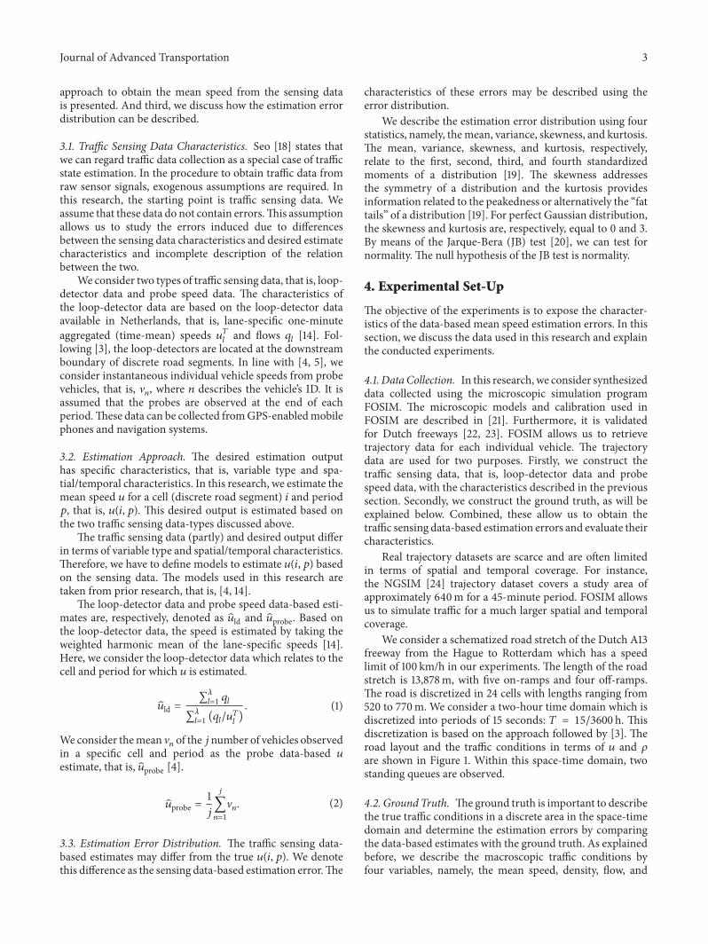
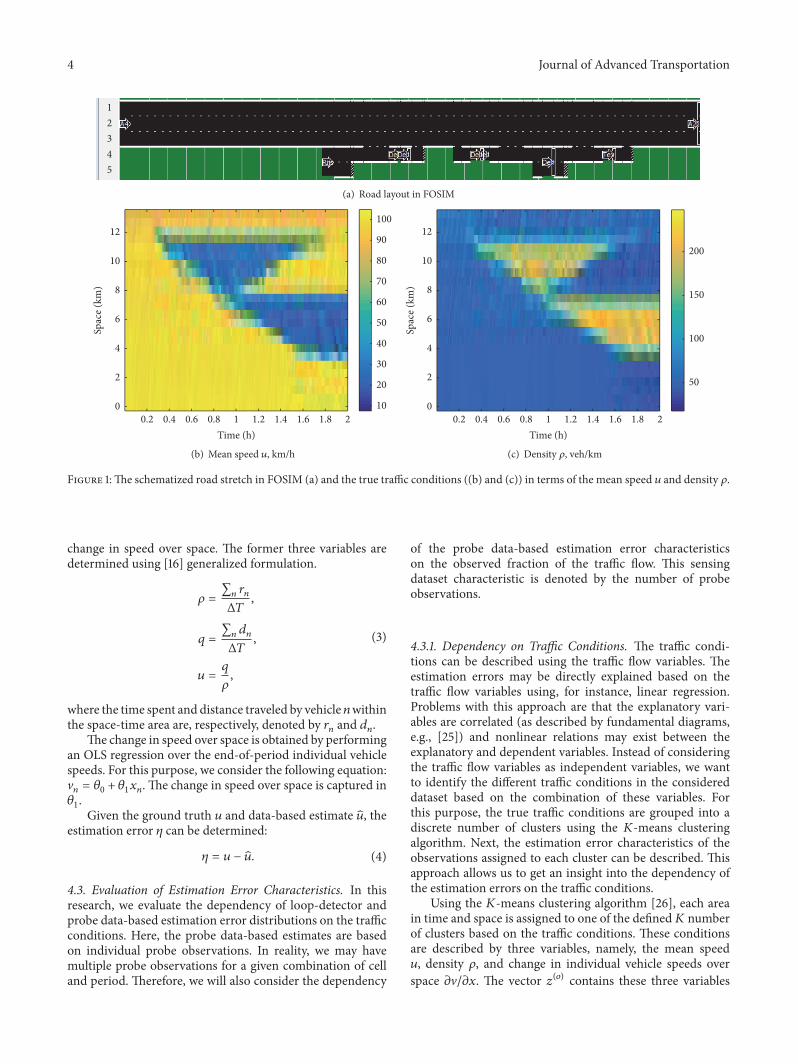
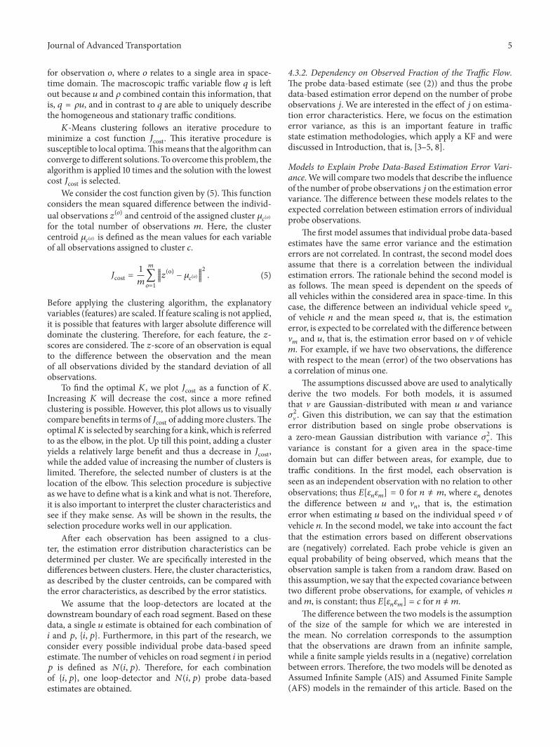
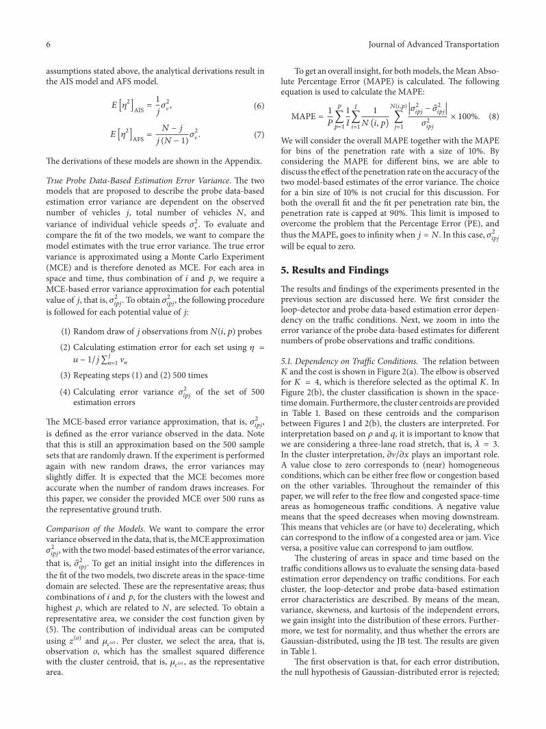
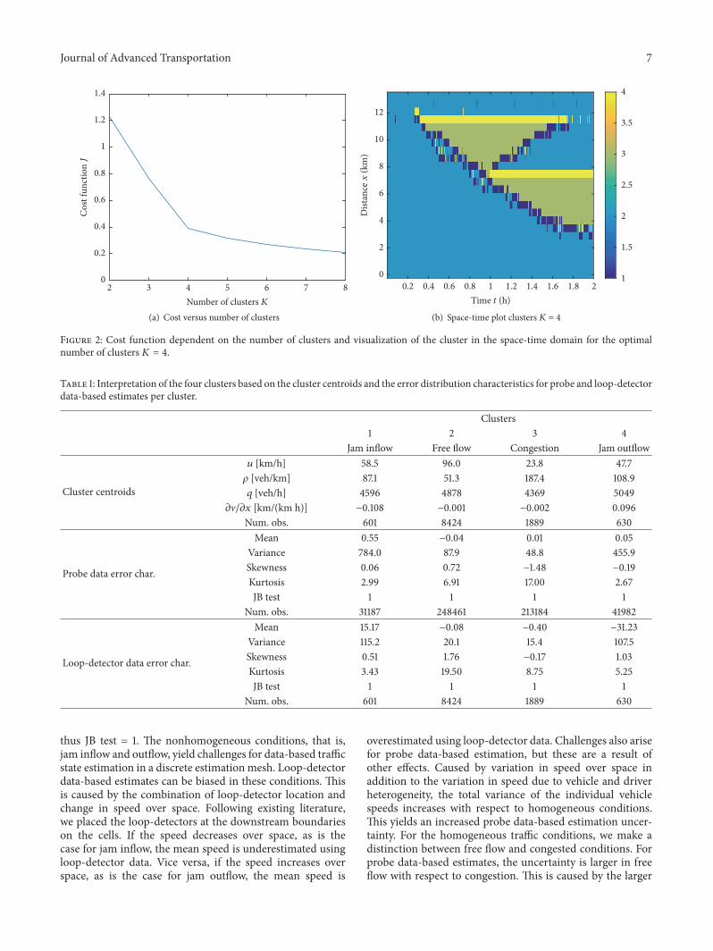
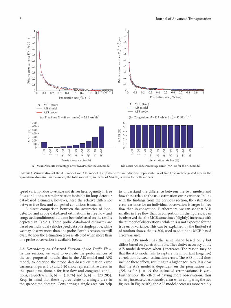
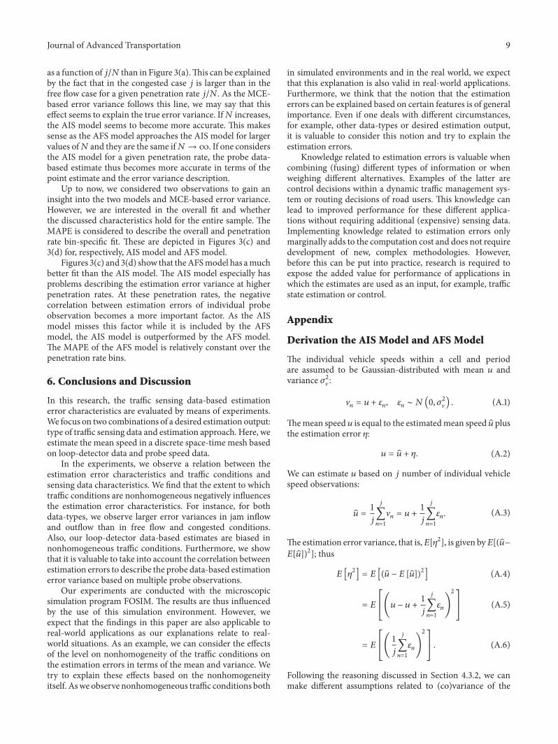