m303 furtherpuremathematics · 2018-06-13 · 2.1 polynomial rings 19 2.2 the degree of a...

M303

Further pure mathematics

Rings and polynomials

This publication forms part of an Open University module. Details of this and otherOpen University modules can be obtained from the Student Registration and Enquiry Service, TheOpen University, PO Box 197, Milton Keynes MK7 6BJ, United Kingdom (tel. +44 (0)845 300 6090;email [email protected]).

Alternatively, you may visit the Open University website at www.open.ac.uk where you can learnmore about the wide range of modules and packs offered at all levels by The Open University.

Note to reader

Mathematical/statistical content at the Open University is usually provided to students inprinted books, with PDFs of the same online. This format ensures that mathematical notationis presented accurately and clearly. The PDF of this extract thus shows the content exactly asit would be seen by an Open University student. Please note that the PDF may containreferences to other parts of the module and/or to software or audio-visual components of themodule. Regrettably mathematical and statistical content in PDF files is unlikely to beaccessible using a screenreader, and some OpenLearn units may have PDF files that are notsearchable. You may need additional help to read these documents.

The Open University, Walton Hall, Milton Keynes, MK7 6AA.

First published 2014. Second edition 2016.

Copyright c© 2014, 2016 The Open University

All rights reserved. No part of this publication may be reproduced, stored in a retrieval system, transmittedor utilised in any form or by any means, electronic, mechanical, photocopying, recording or otherwise, withoutwritten permission from the publisher or a licence from the Copyright Licensing Agency Ltd. Details of suchlicences (for reprographic reproduction) may be obtained from the Copyright Licensing Agency Ltd, SaffronHouse, 6–10 Kirby Street, London EC1N 8TS (website www.cla.co.uk).

Open University materials may also be made available in electronic formats for use by students of theUniversity. All rights, including copyright and related rights and database rights, in electronic materials andtheir contents are owned by or licensed to The Open University, or otherwise used by The Open University aspermitted by applicable law.

In using electronic materials and their contents you agree that your use will be solely for the purposes offollowing an Open University course of study or otherwise as licensed by The Open University or its assigns.

Except as permitted above you undertake not to copy, store in any medium (including electronic storage oruse in a website), distribute, transmit or retransmit, broadcast, modify or show in public such electronicmaterials in whole or in part without the prior written consent of The Open University or in accordance withthe Copyright, Designs and Patents Act 1988.

Edited, designed and typeset by The Open University, using the Open University TEX System.

Printed in the United Kingdom by Halstan & Co. Ltd, Amersham, Bucks.

ISBN 978 1 4730 2036 8

2.1

Contents

Contents

1 Rings 5

1.1 Subrings 11

1.2 Zero divisors and units 13

1.3 Fields 16

2 Polynomials over fields 19

2.1 Polynomial rings 19

2.2 The degree of a polynomial 21

2.3 Basic properties of polynomial rings over fields 23

3 Divisibility of polynomials 25

3.1 Polynomial division 25

3.2 Highest common factors 29

3.3 The Euclidean Algorithm 31

3.4 Least common multiples 33

36Solutions and comments on

exercises

Index 45

1 Rings

1 Rings

In Book B we learnt about groups, which are defined as a set of elementsequipped with some operation ◦, and satisfying certain axioms given inDefinition 1.1 of Book B, Chapter 5. When we think of the set of integers,however, there are two basic operations that we can use: addition, +, andmultiplication, ·. We learnt in Chapter 5 that (Z,+) is an abelian group, What about subtraction and

division? In a sense, we canthink of these as the inverses toaddition and multiplication.

but we can quickly verify that (Z, ·) is not: no integers apart from 1 and−1 have multiplicative inverses and so axiom G3 of Definition 1.1 does nothold.

We may ask which of the group axioms do hold for (Z, ·). If m,n ∈ Z,then m · n ∈ Z and so we have closure (axiom G1). Next, since1 ·m = m · 1 = m, the element 1 ∈ Z acts as the identity to confirmaxiom G2. Finally, associativity of multiplication is a basic property of theintegers and so G4 holds. The integers form a model for our definition of aring.

5


Definition 1.1 Ring axioms

Let R be a set and let + and · be binary operations defined on R.Then (R,+, ·) is a ring if the following axioms hold.The old German word Ring can

mean ‘association’; hence theterms ‘ring’ and ‘group’ havesimilar origins.

Axioms for addition:

R1 Closure For all a, b ∈ R,

a+ b ∈ R.

R2 Associativity For all a, b, c ∈ R,

a+ (b+ c) = (a+ b) + c.

R3 Additive identity There exists an additive identity 0 ∈ R suchthat, for all a ∈ R,

a+ 0 = a = 0 + a.

R4 Additive inverses For each a ∈ R, there exists an additiveinverse −a ∈ R such that

a+ (−a) = 0 = (−a) + a.

R5 Commutativity For all a, b ∈ R,

a+ b = b+ a.

Axioms for multiplication:

R6 Closure For all a, b ∈ R,

a · b ∈ R.

R7 Associativity For all a, b, c ∈ R,

a · (b · c) = (a · b) · c.R8 Multiplicative identity There exists a multiplicative identity

1 ∈ R such that, for all a ∈ R,

a · 1 = a = 1 · a.Axioms combining addition and multiplication:

R9 Distributive laws For all a, b, c ∈ R, multiplication is leftdistributive over addition in R:

a · (b+ c) = (a · b) + (a · c),and multiplication is right distributive over addition in R:

(a+ b) · c = (a · c) + (b · c).Furthermore, (R,+, ·) is a commutative ring if the following extraaxiom holds.

R10 Commutativity For all a, b ∈ R,

a · b = b · a.

6

1 Rings

At first sight, this looks like a lot of individual axioms to satisfy; so let uslook at them collectively. First off, note that the axioms for addition (R1to R5) are exactly the axioms required for (R,+) to be an abelian group.As a result, we can use the ‘Elementary consequences’ (see, for example,Proposition 1.2 of Book B, Chapter 5) to deduce the following.

Lemma 1.2

Let (R,+, ·) be a ring. Then the additive identity 0 ∈ R is unique.Furthermore, for every a ∈ R the additive inverse (−a) is unique.

Next, R6 to R8 tell us some rules about multiplication, but note that it isnot the case that (R, ·) is a group, because we are missing the axiom thatguarantees the existence of multiplicative inverses. Finally, R9 shows ushow to combine these two operations, in exactly the way we expect whenmultiplying and adding integers.

Early definitions of a ring did not include the multiplicative identityaxiom, and this approach persists in some texts. In this case, the ring wehave defined above is called a ring with 1, to distinguish it from a ‘ringwithout 1’. However, all our rings will have a multiplicative identity, andso we can use the term ‘ring’ unambiguously.

Most of the rings in this module will also be commutative (that is, axiomR10 holds), but as we are about to see an example of a non-commutativering, we will not for the moment assume this axiom.

Example 1.3 Some familiar rings

(a) (Z,+, ·), the set of integers Z, with normal addition and This was our original ‘template’to create the abstract definitionof a ring. So it is appropriatethat it is the first example weencounter.

multiplication, is a commutative ring.

To see this, first note that (Z,+) forms an infinite abelian group, withadditive identity 0. This, therefore, immediately covers axioms R1 toR5. Similarly, R6 to R8 follow since multiplication over the integers isclosed, associative, and the multiplicative identity is 1. Of course,multiplication over the integers is commutative, and so we can alsoverify axiom R10. This leaves only axiom R9, which follows asdistributivity is a basic property of the integers.

(b) (Q,+, ·), the set of rational numbers, with normal addition andmultiplication, forms a commutative ring. Similarly, we can readilycheck that the set of real numbers, R, and the set of complex numbers,C, are also both commutative rings under the same operations.

(c) (M2×2,+, ·), the set of 2× 2 matrices over R, with matrix additionand multiplication, is a ring but not a commutative ring.

Checking some of the axioms for this example takes a little morethought. For addition, closure follows since the sum of two 2× 2matrices is another 2× 2 matrix. It can easily be checked that theaddition of matrices is associative and commutative. The additive

7


identity is the zero matrix

(

0 00 0

)

and consequently the additive

inverse of the matrix

(

a b

c d

)

is

(

−a −b

−c −d

)

.

For multiplication, when we multiply two 2× 2 matrices together weobtain another 2× 2 matrix, and so closure (R6) is satisfied. It isstraightforward (but not immediately obvious) to check thatmultiplication is associative, and we can check that the identity matrix(

1 00 1

)

acts as the multiplicative identity for axiom R8.

Finally, axiom R9 can be readily verified, but it is well known thatmultiplication of matrices is not commutative and so R10 does nothold. For example:

(

1 11 0

)

·(

0 11 1

)

=

(

1 20 1

)

, but

(

0 11 1

)

·(

1 11 0

)

=

(

1 02 1

)

.

Exercise 1.1

The ring Z× Z consists of all ordered pairs of integers (a, b), with additionand multiplication defined by (a, b) + (c, d) = (a+ c, b+ d) and(a, b) · (c, d) = (ac, bd). Write down:

(a) (2, 1) + (4, 5) and (2, 1) · (4, 5)(b) the additive identity element

(c) the additive inverse of the element (2, 1)

(d) the multiplicative identity element.

Exercise 1.2

Show that the following are commutative rings.

(a) The set of integers Zn = {0, 1, 2, . . . , n− 1}, equipped with additionand multiplication modulo n.

(b) The set

Z[√2] = {a+ b

√2 : a, b ∈ Z},

equipped with the usual addition and multiplication of real numbers.

You may be wondering how we justify statements such as ‘multiplication ofintegers is associative’. The properties of integers that you have known(not necessarily by name) and used since you first started doing arithmeticcan be justified only by working with a formal definition of the integers. Awell-known definition of the integers starts from a set of axioms known as‘Peano axioms’, after Giuseppe Peano (1858–1932). These are thenextended to give ‘Peano arithmetic’. These axioms include the properties

8

1 Rings

such as associativity, commutativity and distributivity that we have beendiscussing, but in this module you are not expected to be familiar withthese axioms; the approach we have used so far to justify such statementsis sufficient.

In light of the examples above, you may now be wondering what objects donot form rings; so let us look at a couple before we proceed.

Example 1.4 Two examples of non-rings

(a) The set of non-negative integers, Z+ = {0, 1, 2, . . .}, with the usualaddition and multiplication.

We find that R1 and R2 are true, but then we cannot find additiveinverses to satisfy R3: for example, we need −1 to be the additiveinverse of 1, but it is not in the set Z+.

(b) The even integers, 2Z = {. . . ,−4,−2, 0, 2, 4, . . .}, with the usualaddition and multiplication.

In this example, we find that this set does actually form an abeliangroup under addition. The problem comes when we try to find amultiplicative identity for axiom R8: there isn’t one! If there was amultiplicative identity, 2k ∈ 2Z, say, then (2k) · (2n) = 2n for alln ∈ Z. This, however, implies that 2k = 1, and so k 6∈ Z, which is acontradiction.

Having seen some examples and non-examples, we are ready to prove somesimple properties that we should expect to find. Throughout these, youshould be thinking how this is exactly what we expect in the examples ofrings that we have just seen. Are the properties also true for each of ourtwo non-examples, and if they aren’t, why not?

Proposition 1.5 Basic properties of rings

Let (R,+, ·) be a ring. Then:

(a) 0 · a = a · 0 = 0 for all a ∈ R

(b) −(−a) = a for all a ∈ R

(c) a · (−b) = (−a) · b = −(a · b) for all a, b ∈ R

(d) (−a) · (−b) = a · b for all a, b ∈ R.

9


Proof We will prove parts (a)–(c), and leave part (d) as an exercise forProving statements like these isactually quite tricky: we need tobe careful that at each stage weuse only the axioms that definea ring, or results that we havederived from these axioms.

you to do.

(a) Let a ∈ R, and set b = 0 · a. We want to show that b is the additiveidentity. First, we know that 0 = 0 + 0, and so 0 · a = (0 + 0) · a= 0 · a+ 0 · a, using axiom R9. Since we set b = 0 · a, we haveb = b+ b. Therefore, using associativity:

0 = b+ (−b) = (b+ b) + (−b) = b+ (b+ (−b)) = b+ 0 = b.

A similar argument can be used to prove that a · 0 = 0.

(b) First, for any a ∈ R we have (−a) + a = 0. Now, the element (−a) ofR has a unique additive inverse (by Lemma 1.2), namely −(−a), fromwhich it follows that a = −(−a).

(c) We have a · b+ (−a) · b = (a+ (−a)) · b = 0 · b = 0, the last stepfollowing by part (a) of the proposition. Therefore, (−a) · b must bethe additive inverse of a · b, and so we have (−a) · b = −(a · b).Similarly, we can show that −(a · b) = a · (−b).

Having established these basic properties, we will relax our notation alittle. We have so far used the minus sign ‘−’ to denote the additiveinverse of an element: a+ (−a) = 0. When working with the integers, weare familiar with using the minus sign as a binary operation, that is, wewrite expressions such as ‘a− b’. We will extend this notation here.Formally, in any ring R with a, b ∈ R, we define a− b to mean the result ofadding the additive inverse of b to a. Put simply, a− b = a+ (−b).

When the context is clear, we will use two further notationalsimplifications, similar to those made at the start of Book B. First, we willwrite the juxtaposition ab to mean the product a · b. Second, we will oftenrefer to (R,+, ·) by the set symbol R when it is clear which operations arebeing used.

Exercise 1.3

Prove part (d) of Proposition 1.5.

Exercise 1.4

What can you say about a ring in which the additive and multiplicativeidentities are the same, that is, a ring where 0 = 1?

10

1 Rings

1.1 Subrings

In Exercise 1.2, we showed that the sets Zn and Z[√2] were rings. In the

solution, we appealed to properties of addition and multiplication of alarger set to prove some of the axioms. For example, Z[

√2] is a subset of

the ring R, and hence, since we are using the same definition of additionand multiplication for both, some of the axioms hold immediately. In thissubsection, we want to formalise this approach.

Definition 1.6 Subring

Let R be a ring. We say that S is a subring of R if:

(a) the set S is a subset of R

(b) S is a ring when equipped with the same binary operations as R

(c) the ring S has the same multiplicative identity as R.

Why do we insist that S has the same multiplicative identity? As we willsee shortly in Worked Exercise 1.9(b), it is possible for a subset of a ring tobe a ring itself, but with a different multiplicative identity. We want to beable to distinguish between this case and the definition given above.

Why, then, did we not also insist that S should have the same additiveidentity as R? We can deduce this from the definition given above.

Lemma 1.7

Let R be a ring, and S a subring of R. Then the additive identityof S is the same as the additive identity of R.

Proof Suppose 0S is the additive identity in S, and 0R that for R. Thenfor any s ∈ S, we have s+ 0S = s as an equation in S, and so also as anequation in R. Working in R, we now have:

0R = (−s) + s

= (−s) + (s + 0S)

= ((−s) + s) + 0S = 0R + 0S

= 0S .

Some obvious examples are the integers Z as a subring of the rationals Q,and the rationals as a subring of the reals R, and the reals as a subring ofthe complex numbers C. We saw in Example 1.3 that all of Z,Q,R and C

are rings, and for each the additive identity is 0 and the multiplicativeidentity is 1.

Now, as we wanted, we can state and prove a lemma justifying why we donot need to check all the axioms R1–R9 when verifying that a subset of aring is a subring.

11


Lemma 1.8 Subring criterion

Let R be a ring and let S be a subset of R. Then S is a subring of Rif:

SR1 for all s, t ∈ S, s− t ∈ SAxiom SR1 can be thought of as‘closure under subtraction’.

SR2 for all s, t ∈ S, st ∈ S

SR3 the multiplicative identity of R is in S.

Proof Since S is a subset of R, we just need to check that S is a ringwith the same binary operations and multiplicative identity as R.

Let s ∈ S. (Note that S is non-empty by SR3; so such an s exists.) BySR1, s− s = 0 ∈ S and so 0− s = (−s) ∈ S. In addition, if t ∈ S then(−t) ∈ S, so that s+ t = s− (−t) ∈ S. This shows that (S,+) is anabelian subgroup of (R,+).

Multiplication is closed in S by SR2, and axiom SR3 ensures that themultiplicative identity of R is in S, and in fact it must be a multiplicativeidentity for S. The associative and distributive laws hold since they holdin R. Thus we have shown that S is a ring, and since the multiplicativeidentity coincides, it follows immediately that S is a subring of R.

Worked Exercise 1.9

(a) Show that the set of Gaussian integers,Z[i] = {a+ ib : a, b ∈ Z} where i =

√−1, equipped with the usual

addition and multiplication of complex numbers, is a ring.

(b) Why is S = {0, 5} not a subring of Z10?

Solution

(a) Since Z[i] is a subset of the complex numbers C, it will be enoughto prove that Z[i] is a subring of C. We check the conditions ofLemma 1.8. Consider two elements a+ ib and c+ id of Z[i]. Then

SR1: (a+ ib)− (c+ id) = (a− c) + i(b− d) ∈ Z[i].

SR2: (a+ ib) · (c+ id) = (ac− bd) + i(ad+ bc) ∈ Z[i].

SR3: The multiplicative identity of C and Z[i] is 1 = 1 + 0i.

It follows from the subring criterion that Z[i] is a subring of C,and therefore that Z[i] is a ring.

(b) Condition SR3 does not hold for S: the multiplicative identity ofZ10 is 1, which is not in S.

Note, however, that S is a ring with the same operations as Z10.The multiplicative identity of S is 5.

12

1 Rings

The requirement that the multiplicative identity of a subring is always thesame as that of the original ring has some interesting consequences. Forexample, the only subring of Z is Z itself, and the only subring of Zn is Zn.

Exercise 1.5

By considering a suitable larger ring and using Lemma 1.8, prove that thefollowing are rings:

(a) Z[ω] = {a+ bω+ cω2 : a, b, c ∈ Z} where ω = e2iπ/3, so that ω3 = 1

(b) Q[i] = {a+ bi : a, b ∈ Q}.

1.2 Zero divisors and units

The axioms that define a ring leave some opportunities for results that wemight not expect. By considering the integers Z, we already know thatelements do not need to have multiplicative inverses, but in some ringseven stranger things can happen.

Suppose that in Z we wish to solve the quadratic equation

x2 − 5x+ 6 = 0.

Factorising the left-hand side, we obtain

(x− 2)(x− 3) = 0.

It follows that either x− 2 = 0 or x− 3 = 0, and hence that x = 2 orx = 3. This method works since if in Z the product of two terms is 0, thenone of the two terms must itself be 0.

More generally, if we know that the product of two integers a and b is 0,then we can deduce that at least one of a or b must be 0. Put another way,if we multiply two non-zero integers then their product must also benon-zero.

However, in the ring Z6 we have 2 · 3 ≡ 0 (mod 6). In other words, thereare two non-zero elements whose product is zero. We want to be able todistinguish between elements where this does happen and those where itdoes not, and so we make the following definition.

Definition 1.10 Zero divisor

Let R be a ring. A non-zero element a ∈ R is a zero divisor in R ifthere is a non-zero element b ∈ R for which ab = 0 or ba = 0.

In a sense, 0 is also a zero divisor since 0 · 1 = 0 is true in every ring, butwe have deliberately excluded this so that in future we do not have to keepusing phrases such as ‘no non-zero zero divisors’. Commutative rings withno zero divisors have a special name. Since they have several of the We will learn more about

integral domains in Chapter 12.properties of the ring of integers, we call them integral domains.

13


Example 1.11 Rings with no zero divisors

(a) The ring Z has no zero divisors – this is the fact that we used to solvethe quadratic equation above. Similarly, Q, R and C also have no zerodivisors.

(b) Z7 has no zero divisors. If ab ≡ 0 (mod 7), then 7 divides ab, and hence(since 7 is prime) divides a or b (or both) in Z7. Thus a = 0 or b = 0.

Example 1.12 Rings with zero divisors

(a) Z6, as we saw above, does have zero divisors. Since 2 · 3 ≡ 0 (mod 6)and 3 · 4 ≡ 0 (mod 6), we see that all of 2, 3 and 4 are zero divisors.

However, 1 and 5 are not zero divisors since there are no numbers aand b (other than 0) in Z6 for which 1 · a ≡ 0 (mod 6) or5 · b ≡ 0 (mod 6).

(b) The ring M2×2 of 2× 2 matrices with entries from R has zero divisors.For example, the product

(

1 00 0

)

·(

0 00 1

)

=

(

0 00 0

)

shows that both

(

1 00 0

)

and

(

0 00 1

)

are zero divisors.

Exercise 1.6

Let R be the ring Z× Z (as defined in Exercise 1.1). For a, b, c, d ∈ Z,addition is defined by (a, b) + (c, d) = (a+ c, b+ d), and multiplication isgiven by (a, b) · (c, d) = (ac, bd).

(a) Give an example of a zero divisor in R.

(b) Describe all the zero divisors in R.

Now that we are aware of the possibility that rings have zero divisors, weturn again to the issue of multiplicative inverses: which elements of a ringcan be multiplied together to give 1? For example, in Z, we have(−1) · (−1) = 1, and so −1 is its own multiplicative inverse, but there is nomultiplicative inverse of 2 in Z.

So far, we have allowed our rings to be non-commutative, that is, axiomR10 has not needed to be satisfied. Our main example of anon-commutative ring has been M2×2, the ring of 2× 2 matrices withentries from R. As we move our focus to consider elements that havemultiplicative inverses, the existence of non-commutative rings leads tosome awkward possibilities. For example, could we have anon-commutative ring R and a, b ∈ R, with a · b = 1, but b · a 6= 1?The answer to this question is

‘yes’ for some quite peculiarrings, but we will not explorethis here.

14

1 Rings

Convention: commutative rings

To avoid the complications described above, all rings we will considerfrom now on will be commutative. Additionally, we will drop theword ‘commutative’ and simply use the term ‘ring’.

With this settled, we can define a term for elements that havemultiplicative inverses.

Definition 1.13 Unit

An element a of a (commutative) ring R is a unit if there is an The term ‘unit’ is overused inmathematics generally. It shouldbe clear from the context whichmeaning is appropriate.

element a−1 ∈ R for which a · a−1 = a−1 · a = 1.

For example, in the ring Z the only units are 1 and −1; in the ring Z10 theunits are 1, 3, 7 and 9, since

1× 1 ≡ 1 (mod 10), 3× 7 ≡ 1 (mod 10) and 9× 9 ≡ 1 (mod 10).

Exercise 1.7

List all the units in the following rings.

(a) Z12

(b) Z× Z

(c) Z[i]

Although in the above exercise it was relatively straightforward to list theunits in specific rings, this is not always the case. We will see examples inChapter 12 where finding units is rather more difficult.

Exercise 1.8

(a) Write down all the zero divisors in the rings Zn, for n = 8, 9, 10, 11and 12.

(b) Give a description of all the zero divisors in Zn, for any given naturalnumber n.

(c) Which rings Zn have no zero divisors?

(d) Show that in a ring R, if a is a unit then it cannot be a zero divisor.

15


1.3 Fields

In the definition of a ring, the axiom we were missing for the non-zeroelements to form a group under multiplication was that every element hasan inverse: in other words, every non-zero element is a unit. A ring withthis property is called a field.

Definition 1.14 Field

A (commutative) ring R is a field if the additive and multiplicativeRecall Exercise 1.4, which tellsus what happens when 0 = 1 ina ring.

identities are distinct, and every non-zero element is a unit.

In other words, R has distinct elements 0 and 1, axioms R1–R10 hold,and so does:

R11 Multiplicative inverses For every non-zero a ∈ R, thereexists a−1 ∈ R such that a · a−1 = a−1 · a = 1.

In the same way that we have been using the symbol R to refer to a generalring, we will use F for a field. You may find that in other texts the letterK is used: this is because the German mathematician Richard Dedekind(1831–1916) used the term Korper for field, which translates as ‘body’.

Example 1.15 Some well-known fields

The following are easily seen to be fields.

(a) Q: Since pq ·

qp = 1 for non-zero p, q ∈ Z, the inverse of p

q is qp .

(b) R: The inverse of any non-zero x ∈ R is x−1 = 1x .

(c) C: The inverse of z = a+ ib 6= 0 is

z−1 =1

a+ ib=

(

a

a2 + b2

)

+ i

( −b

a2 + b2

)

.

Example 1.16 Some rings that are not fields

(a) Z is not a field: as we observed in the previous subsection, the onlyunits are −1 and 1, and so no other integer has a multiplicative inverse.

(b) Z6 is not a field: for example, the element 2 is not a unit.

Since Z6 has sufficiently few elements, we can verify this by testing allmultiples of 2 modulo 6:

2 · 0 ≡ 0, 2 · 1 ≡ 2, 2 · 2 ≡ 4,

2 · 3 ≡ 0, 2 · 4 ≡ 2, 2 · 5 ≡ 4.

16

1 Rings

Exercise 1.9 Properties of multiplicative inverses

Let F be a field, and a, b ∈ F non-zero elements. Prove the following.

(a) (a−1)−1 = a

(b) (ab)−1 = b−1a−1

The second example of a non-field, Z6, raises an interesting point: we usedthe element 2, which is a zero divisor, since 2 · 3 ≡ 0 (mod 6). InExercise 1.8(d), we showed that any element that is a unit cannot also be azero divisor. As a consequence of this, we have the following lemma.

Lemma 1.17

Let F be a field. Then F has no zero divisors.

Proof Suppose a 6= 0 is a zero divisor in F , and so there exists anon-zero b ∈ F such that a · b = 0. By axiom R11, there exists b−1 ∈ F

such that b · b−1 = 1. Now

a = a · 1 = a · (b · b−1) = (a · b) · b−1 = 0 · b−1 = 0,

which is a contradiction.

In Exercise 1.8, we stated that Zn has no zero divisors if, and only if, n is aprime number. In fact, each element of Zn is either a zero divisor or a unit.

Lemma 1.18

Let a ∈ Zn be non-zero, where n ∈ N. Then a is either a zero divisoror a unit.

Proof If hcf(a, n) = 1, then by Proposition 4.7 of Book A, Chapter 1 For any non-zero element a, oneof two things can happen: eitherhcf(a, n) = 1, or hcf(a, n) > 1.We consider each of thesepossibilities in turn.

there exist s, t ∈ Z such that sa+ tn = 1. Therefore, sa ≡ 1 (mod n), andhence a is a unit in Zn.

On the other hand, if hcf(a, n) = d > 1, then a = dh and n = dk for someh, k, with 1 < k < n and hcf(h, k) = 1. Then

ak = (dh)k = (hd)k = h(dk) = hn ≡ 0 (mod n),

which proves that a is a zero divisor.

This lemma immediately gives us an important consequence.

Corollary 1.19

The ring Zn is a field if, and only if, n is a prime number.

17


The fields Zp, where p is a prime number, contain only finitely manyelements, and are therefore called finite fields. We will not explore finitefields further in this chapter, as we will study them in some detail inBook E, Chapter 19. However, we will make two quick remarks.

First, the fields Zp, for p prime, are not the only finite fields: in fact, thereexists a finite field with q elements if, and only if, q is a power of a primenumber.

Second, if we repeatedly add the multiplicative identity to itself,1 + 1 + · · ·+ 1, we will at some point end up with the additive identity.For example, in Z3, 1 + 1 + 1 = 3 ≡ 0 (mod 3). The number of times weadd 1 to itself to get 0 is known as the characteristic. So, thecharacteristic of Z3 is 3.

We finish this section by defining subfields, and developing an analogue tothe subring criterion (Lemma 1.8) that allows us to avoid checking all theaxioms.

Definition 1.20 Subfield

A subset S of a field F that is a field with the same binary operationsand multiplicative identity as F is known as a subfield of F .

Lemma 1.21 Subfield criterion

Let F be a field, and let S be any subset of F . Then S is a subfield ofF if:

(a) S is a subring of F

(b) every non-zero element of S has a multiplicative inverse in S.

Consequently, to determine whether S is a subfield of F or not, we need tocheck only axioms SR1–SR3 from Lemma 1.8 and axiom R11 fromDefinition 1.14.

Proof Since S is a subset of F , we just need to check that S is a fieldwith the same binary operations and identities as F . First, condition (a)tells us that S has the same multiplicative identity as F , and that all theaxioms R1–R10 hold. This leaves only axiom R11 about the existence ofmultiplicative inverses, but this is guaranteed by condition (b).

Exercise 1.10

By considering suitable larger fields, show that the following are fields.

(a) Q[i] = {a+ bi : a, b ∈ Q}(b) Q[

√2] = {a+ b

√2 : a, b ∈ Q}

18

2 Polynomials over fields


As we saw in Subsection 1.2, rings can have unexpected properties. Toavoid some of these issues, we are going to spend the remainder of thischapter studying polynomial rings where the coefficients of thepolynomials come from a field, as these are generally much better behavedthan generic rings.

2.1 Polynomial rings

Definition 2.1 Polynomial ring over a field

Let F be a field. Then a polynomial over F with the variable x is apolynomial of the form f(x) = a0 + a1x+ a2x

2 + · · ·+ anxn, where

a0, a1, a2, . . . , an ∈ F and n ≥ 0, where x0 is defined to be 1.

The polynomial ring over F is

F [x] = {a0 + a1x+ · · ·+ anxn : a0, a1, . . . , an ∈ F, n ≥ 0}.

We have seen the square bracket notation ‘F [x]’ a few times already in thischapter, and it is worth verifying that our use of it has been consistent.For example, in Exercise 1.10(b) we encountered Q[

√2], which was defined

to be the set {a+ b√2 : a, b ∈ Q}. The above definition would define it as

{a0 + a1√2 + · · ·+ an(

√2)n : ai ∈ Q}, but of course (

√2)2 = 2 is already

an element of Q, and so the higher terms of√2 can simply be included in

the coefficients a0 and a1.

To be clear that F [x] is indeed a ring, we need to define ‘addition’ and‘multiplication’ within F [x], and then be sure that all the axioms hold.How we add and multiply polynomials should come as no surprise: first,we need to remember that the field F came with its own addition andmultiplication, and use these to build the natural definitions. If in doubt,think about how it is done in R[x], that is, when the coefficients are all realnumbers.

Addition is defined by(

n∑

i=0

aixi

)

+

(

m∑

i=0

bixi

)

=

max(m,n)∑

i=0

(ai + bi)xi.

Note that the sum on the right-hand side of this equation goes up tomax(m,n): so, if n < m then we add ‘dummy’ coefficientsan+1 = an+2 = · · · = am = 0.

What is the zero of F [x]? If ‘0’ is the symbol for the zero in the field F ,then let 0x be the zero in F [x]. It is defined as the polynomial where everycoefficient is equal to 0; so in fact we have 0x = 0. However, we willcontinue to use the symbol 0x to highlight when we are working in thepolynomial ring F [x].

19


We can now work out additive inverses:(

n∑

i=0

aixi

)

+

(

n∑

i=0

(−ai)xi

)

=

n∑

i=0

(ai + (−ai)) xi = 0x.

The closure, associativity and commutativity of addition in F [x] followquite easily: remember that we can assume they hold in F .

Next, we define multiplication:(

n∑

i=0

aixi

)

·

m∑

j=0

bjxj

=

m+n∑

k=0

∑

i+j=k

ai · bj

xk.

At first sight, this definition looks rather offputting. So, let us quicklyconsider an example to reassure ourselves that this is exactly what weexpect to see. Take polynomials f(x) = 1 + 5x− 4x2 and g(x) = 2 + 3xover R. Then

f(x)g(x) = (1 + 5x− 4x2) · (2 + 3x)

=(

1 · 2)

+(

1 · 3 + 5 · 2)

x+(

5 · 3 + (−4) · 2)

x2 +(

(−4) · 3)

x3

= 2 + 13x + 7x2 − 12x3.

What is the multiplicative identity of F [x]? As we did with the zero, wewill use the special symbol 1x to distinguish it from the ‘1’ in F , eventhough 1x = 1.

The remaining axioms R6–R9 are readily verified, as a consequence of theaxioms for the field F . In addition, since multiplication in F iscommutative, it follows that F [x] is a commutative ring, that is, axiomR10 holds.

Example 2.2 Some common polynomial rings

(a) The set of polynomials with rational coefficients, Q[x], with 0x = 0 andThe polynomial ring Q[x] willappear in Section ??. 1x = 1, is a ring since Q is a field.

(b) C[x] represents the polynomials with complex coefficients, and R[x]the polynomials with real coefficients. Note that Q[x] ⊂ R[x] ⊂ C[x].

(c) The polynomial ring Z2[x] consists of all polynomials whosecoefficients are all either 0 or 1. More generally, we can consider thepolynomial ring Zp[x] where p is a prime number.

20


Worked Exercise 2.3

Let f(x) = 1 + 2x and g(x) = 1 + 3x+ 2x3 be polynomials in Z5[x],the ring of polynomials over the field Z5, equipped with addition andmultiplication modulo 5.

(a) Calculate and simplify (i) f(x) + g(x), and (ii) 3f(x)− g(x).

(b) Compute f(x)g(x).

Solution

(a) (i) f(x) + g(x) = (1 + 1) + (2 + 3)x+ 2x3 ≡ 2 + 2x3 (mod 5)

3f(x)− g(x) = 3(1 + 2x)− (1 + 3x+ 2x3)(ii)

= (3 + (3× 2)x)− 1− 3x− 2x3

≡ (3 + x) + 4 + 2x+ 3x3

= (3 + 4) + (1 + 2)x+ 3x3

≡ 2 + 3x+ 3x3 (mod 5)

f(x)g(x) = (1 + 2x)(1 + 3x+ 2x3)(b) Note that it is sometimes easierwhen working in Zp[x] tocalculate the polynomials overZ, and then reduce thecoefficients modulo p at the end.

= 1 + 5x+ 6x2 + 2x3 + 4x4

≡ 1 + x2 + 2x3 + 4x4 (mod 5)

Exercise 2.1

Let f(x) = 2x3 − 3 and g(x) = 9x4 + 7x2 − x+ 1. Compute (i) f(x) + g(x)and (ii) f(x) · g(x) in the following polynomial rings:

(a) Q[x]

(b) Z7[x]

(c) Z2[x].

2.2 The degree of a polynomial

Definition 2.4 Degree of a polynomial

Let F be a field, and let f(x) = a0 + a1x+ · · ·+ anxn be a

polynomial in F [x]. The degree of f(x), deg(f), is the largest k ≥ 0for which ak 6= 0.

This non-zero coefficient ak is known as the leading coefficient.

21


At this point, it is also worth making a remark about notation: strictlyspeaking, we should have written deg(f(x)) rather than deg(f), but this israther clumsy. For the same reason, in future we will occasionally dropthe ‘(x)’ from other equations involving polynomials, where the meaning isstill sufficiently clear.

Example 2.5 The degree of a polynomial

In Exercise 2.1, the polynomial f(x) = 2x3 − 3 has degree 3 in Q[x] andZ7[x], but f(x) ≡ 1 (mod 2) and so f(x) has degree 0 in Z2[x].

On the other hand, the polynomial g(x) = 9x4 + 7x2 − x+ 1 has degree 4in all of Q[x], Z7[x] and Z2[x].

Convention: degree of the zero polynomial

By convention, the degree of the polynomial 0x will be −∞, whichshould be interpreted as meaning we can choose the degree of 0x to beas largely negative as we need.

This choice is made so that the following lemma is consistent when one orboth of the polynomials f and g are equal to 0x.

Lemma 2.6

Let F be a field, and let f(x) and g(x) be polynomials in F [x]. Thendeg(fg) = deg(f) + deg(g).

This seemingly innocuous lemma actually turns out to be quite important,as we will see later in this chapter and the next. Before we prove it, let uspause to think what would happen if we replaced the field F with somearbitrary ring R. We consider an example in the following exercise.

Exercise 2.2

Consider the polynomials f(x) = 2x2 + x+ 3 and g(x) = 3x+ 1 in thepolynomial ring Z6[x]. Find:

(a) deg(f)

(b) deg(g)

(c) deg(fg).

What went wrong? We expected the degree of f(x)g(x) to be 3, but thecoefficient of x3 disappeared because 2 · 3 ≡ 0 (mod 6). This, of course, isbecause 2 and 3 are zero divisors in Z6, and we know from Lemma 1.17that fields cannot have zero divisors.

22


Proof of Lemma 2.6 First, if either f(x) or g(x) is equal to 0x, thenfg = 0x and deg(fg) = −∞ as we should expect. So we now suppose thatf(x) 6= 0x and g(x) 6= 0x.

Let f(x) = a0 + a1x+ · · · + anxn and g(x) = b0 + b1x+ · · ·+ bmxm be

polynomials over F , where deg(f) = n and deg(g) = m. In particular, thismeans that an 6= 0 and bm 6= 0. Now, from the definition of multiplicationin F [x],

f(x)g(x) =

m+n∑

k=0

∑

i+j=k

ai · bj

xk.

The highest term in this sum is anbmxm+n, and so we certainly havedeg(fg) ≤ deg(f) + deg(g). Moreover, since an, bm ∈ F are both not equalto zero, it follows by Lemma 1.17 that their product anbm is also not 0.Thus deg(fg) = m+ n = deg(f) + deg(g).

Meanwhile, what happens to the degree if we add two polynomials?Clearly, from the definition, deg(f + g) ≤ max(deg(f),deg(g)), but can wereplace the ‘≤’ with ‘=’? Again, let us first consider a couple of examples.

Exercise 2.3

Calculate the degree of f(x) + g(x) over the stated ring:

(a) f(x) = 2x3 + 4x2 − 1 and g(x) = 3x3 + 3x2 − 2x over Z5

(b) f(x) = 1 + x and g(x) = 1− x over Q.

In the above exercise, you should have found that it is indeed possible forthe degree of the sum of two polynomials to be less than the sum of thedegrees. In each case, the top term of f + g disappeared becausedeg(f) = deg(g), and the leading coefficients of f and g were additiveinverses of each other.

Lemma 2.7

Let F be a field, and let f(x) and g(x) be polynomials in F [x]. Thendeg(f + g) ≤ max(deg(f),deg(g)).

Proof This follows directly from the definition of addition forpolynomials in F [x].

2.3 Basic properties of polynomial rings over fields

Now we have defined and developed the concept of the degree of apolynomial, we are in a position to prove some results to reassure us thatpolynomials over fields behave in the way that we expect them to.

23


First, the property that the field F has no zero divisors can be shown toimply that there are also no zero divisors in F [x].

Lemma 2.8

Let F be a field, and let f(x), g(x) ∈ F [x] be polynomials such thatf(x)g(x) = 0x. Then either f(x) = 0x, or g(x) = 0x (or both).

Proof Since by Lemma 2.6 we have −∞ = deg(0x) = deg(fg)= deg(f) + deg(g), it follows that at least one of f(x) or g(x) must havedegree −∞, that is, f(x) = 0x or g(x) = 0x.

We might now wonder whether in fact F [x] is a field: is every element aunit? This turns out not to be the case.

Lemma 2.9

An element of a polynomial ring F [x] over a field F has amultiplicative inverse (that is, the element is a unit) if, and only if, ithas degree 0.

Proof First, a polynomial f(x) of degree 0 is simply a non-zero elementof the field F : f(x) = a0 with a0 ∈ F . Since F is a field, there existsa−10 ∈ F such that a0 · a−1

0 = 1. Therefore, the inverse of f(x) in F [x] is

f−1(x) = a−10 .

Conversely, for a polynomial f(x) ∈ F [x], suppose that g(x) ∈ F [x] is themultiplicative inverse. Then f(x)g(x) = 1x, and so by Lemma 2.6deg(f) + deg(g) = deg(1x) = 0. By definition, the degree of a polynomial iseither −∞ or an integer value greater than or equal to 0. So the onlypossible situation in which deg(f) + deg(g) = 0 arises is when f hasdegree 0.

Since every unit in a polynomial ring F [x] is actually in F , we willtypically refer to u ∈ F [x] rather than u(x) ∈ F [x] from now on.

Lemma 2.9 implies that F [x] is not itself a field, since we cannot findinverses for anything with degree ≥ 1. However, despite this lack ofinverses in F [x], we can still cancel terms from equations.

Lemma 2.10 Cancellation of polynomials

If f(x) is a non-zero polynomial and f(x)g(x) = f(x)h(x) in F [x],then g(x) = h(x).

24

3 Divisibility of polynomials

Proof We can rearrange the equation fg = fh to obtain fg − fh = 0,which by distributivity gives us f(g − h) = 0. Now g − h is a polynomialover F , so by Lemma 2.8 either f(x) = 0x (which by assumption is nottrue), or g(x) − h(x) = 0x. Therefore, we must have g(x) = h(x).

We finish this section with a couple of definitions that we will need later inthis chapter.

Definition 2.11 Associate and monic

Let F be a field, and f(x), g(x) ∈ F [x].

(a) We say that f(x) is an associate of g(x) if f(x) = ug(x) where u We will generalise the concept of‘associate’ to other rings inChapter 12.

is a unit in F [x].

(b) The polynomial f(x) is monic if the leading coefficient is equalto 1.

Exercise 2.4

Let F be a field, and f(x) a non-zero polynomial in F [x]. Prove thefollowing.

(a) If g(x) ∈ F [x] is an associate of f(x), then deg(g) = deg(f).

(b) There exists a unique monic polynomial that is an associate of f(x).


This section seeks to develop some results concerning the divisibility ofpolynomials that mirror results in Book A, Chapter 1 for the integers.

3.1 Polynomial division

You may already have had practice at dividing one polynomial over thereal numbers by another and calculating the remainder. Here, we want toextend this ‘long division’ to polynomials over an arbitrary field F . Beforewe do this, however, we should justify that what we are doing is valid, andcan be done in a unique way: what we need is a division algorithm forpolynomials, to mirror Theorem 4.1 in Book A, Chapter 1. In fact, as weproceed through this section you may like periodically to glance back atSection 4 of Chapter 1, and observe the similarities.

25


Theorem 3.1 Division Algorithm for polynomials

Let F be a field and let f and g be polynomials in F [x], with g 6= 0x.Then there exist unique polynomials q and r in F [x] such that

(a) deg(r) < deg(g), and

(b) f = qg + r.

The polynomials q and r are respectively known as the quotient andremainder when dividing f by g.

Proof If f = 0x or deg(f) < deg(g), then we can simply take q = 0x andThere are two parts to thisproof. First, we prove theexistence of a suitable q and rusing induction, and then weprove that they are unique.

r = f(x). Thus from now on we will assume deg(f) ≥ deg(g). Letf(x) = a0 + a1x+ · · ·+ anx

n and g(x) = b0 + b1x+ · · ·+ bmxm, withan 6= 0 and bm 6= 0 so that deg(f) = n and deg(g) = m. We use inductionon d = n−m ≥ 0 to prove the existence of a suitable q(x) and r(x).

The base case is d = 0, when m = n. In this case, we can take q = anb−1m ,Remember F is a field, and so

we can find b−1m such that

bmb−1

m = 1.and r = f − qg. Note that deg(r) < deg(g) because the coefficient of xm

in r disappears: am − amb−1m bm = 0.

For the inductive step, suppose that the statement is true ford = 0, 1, . . . , k − 1. Now consider d = k. Define f1 = f − anb

−1m xkg. ThereWe have expressly constructed

f1 so that deg(f1) < deg(f). are three cases to consider: f1 = 0x, deg(f1) < deg(g) anddeg(f1) ≥ deg(g). If f1 = 0x, then we take q = anb

−1m xn−m and r = 0x. If

deg(f1) < deg(g), then we take q = anb−1m xn−m and r = f1. Thus we now

suppose deg(f1) ≥ deg(g). By induction, we can find q1(x), r1(x) such thatf1 = q1g + r1, with deg(r1) < deg(g). We now substitute back:

f = anb−1m xn−mg + f1

= anb−1m xn−mg + (q1g + r1)

=(

anb−1m xn−m + q1

)

g + r1

and so we take q = anb−1m xn−m + q1 and r = r1.

For uniqueness of q and r, suppose that we can find another pair ofpolynomials q∗, r∗ with f = q∗g + r∗. Then we have qg + r = q∗g + r∗,which can be rearranged to give (r − r∗) = (q∗ − q)g. Applying Lemma 2.6,we get deg(r − r∗) = deg(q∗ − q) + deg(g), but since deg(g) > deg(r − r∗)this is a contradiction unless r = r∗ and q∗ = q.

Actually finding q and r, when working in a polynomial ring, requires longdivision of polynomials. We will work through the steps of one example, incase you are not familiar with the process or need reminding.

26


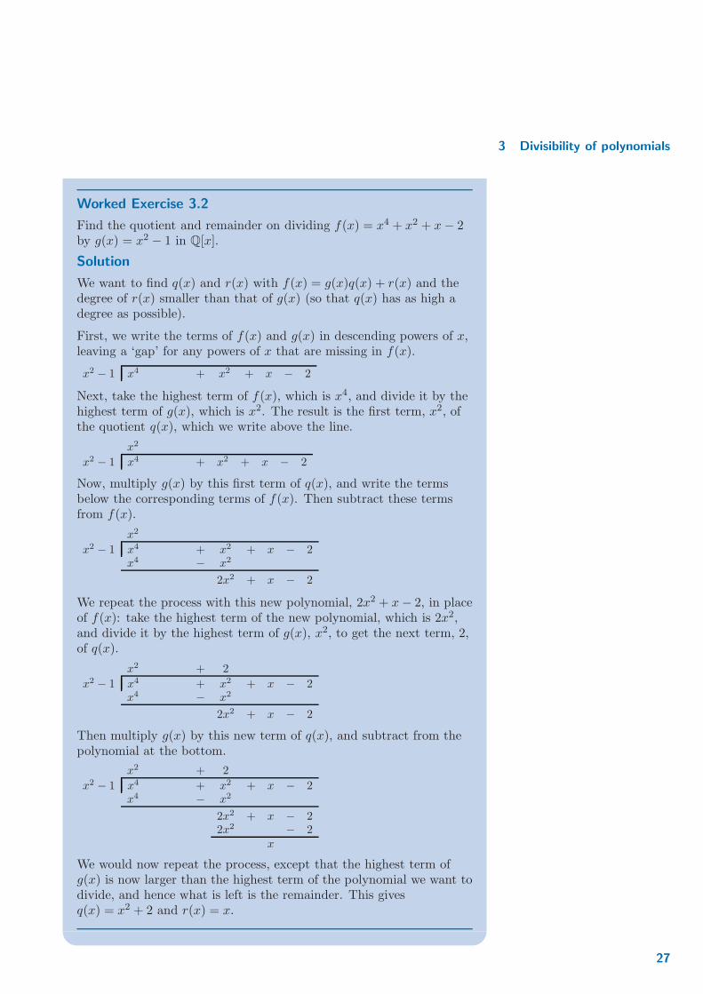
Worked Exercise 3.2

Find the quotient and remainder on dividing f(x) = x4 + x2 + x− 2by g(x) = x2 − 1 in Q[x].

Solution

We want to find q(x) and r(x) with f(x) = g(x)q(x) + r(x) and thedegree of r(x) smaller than that of g(x) (so that q(x) has as high adegree as possible).

First, we write the terms of f(x) and g(x) in descending powers of x,leaving a ‘gap’ for any powers of x that are missing in f(x).

x2 − 1 x4 + x2 + x − 2

Next, take the highest term of f(x), which is x4, and divide it by thehighest term of g(x), which is x2. The result is the first term, x2, ofthe quotient q(x), which we write above the line.

x2

x2 − 1 x4 + x2 + x − 2

Now, multiply g(x) by this first term of q(x), and write the termsbelow the corresponding terms of f(x). Then subtract these termsfrom f(x).

x2

x2 − 1 x4 + x2 + x − 2x4 − x2

2x2 + x − 2

We repeat the process with this new polynomial, 2x2 + x− 2, in placeof f(x): take the highest term of the new polynomial, which is 2x2,and divide it by the highest term of g(x), x2, to get the next term, 2,of q(x).

x2 + 2

x2 − 1 x4 + x2 + x − 2x4 − x2

2x2 + x − 2

Then multiply g(x) by this new term of q(x), and subtract from thepolynomial at the bottom.

x2 + 2

x2 − 1 x4 + x2 + x − 2x4 − x2

2x2 + x − 22x2 − 2

x

We would now repeat the process, except that the highest term ofg(x) is now larger than the highest term of the polynomial we want todivide, and hence what is left is the remainder. This givesq(x) = x2 + 2 and r(x) = x.

27


Exercise 3.1

For each of the following polynomials f(x), g(x) in Q[x], find the quotientq(x) and the remainder r(x) for the division of f(x) by g(x).

(a) f(x) = x3 − 2x2 + 3x− 1, g(x) = x− 1

(b) f(x) = 2x4 − x+ 1, g(x) = x2 + 1

(c) f(x) = 3x3 − 2x2 + 1, g(x) = 2x+ 1

With a division algorithm in hand, we now state precisely what we meanwhen we say that one polynomial divides another: the remainder in theabove process must equal the zero polynomial 0x in F [x].

Definition 3.3 Factors of a polynomial

Let F be a field, and f, g polynomials in F [x]. We say that gdivides f (or g is a factor of f) if there is some polynomial h ∈ F [x],such that f = gh.

If f is non-zero and neither g nor h are units then g and h areproper factors of f .

Notice that if g and h are proper factors of f in F [x], then0 < deg(g) < deg(f) and 0 < deg(h) < deg(f): if deg(g) = 0 then g ∈ F

would be a unit, while if deg(g) = deg(f) then Lemma 2.6 of this chapterwould imply deg(h) = 0, and so h would be a unit.

Once again, the zero polynomial 0x behaves slightly differently: everypolynomial is a factor of 0x since 0x = f(x) · 0x. The following exercise willenable you to develop properties of polynomial division that are directlyanalogous to those we proved for the integers in Section 4 of Book A,Chapter 1.

Exercise 3.2 Properties of division for polynomials

Let F be a field, and let f, g and h be non-zero polynomials in F [x]. Provethe following statements.

(a) If g divides f then g divides f + gh for any polynomial h ∈ F [x].

(b) If h divides g and g divides f then h divides f .

(c) If h divides f and h divides g then h divides af + bg for anypolynomials a, b ∈ F [x].

(d) The polynomials f and g are associates if, and only if, g divides fand f divides g.

28


3.2 Highest common factors

We have now laid the foundations we need to enable us to describe theanalogue of the Euclidean Algorithm for polynomials, and hence developthe concept of highest common factor. We proceed in exactly the sameway as we did for the integers in Book A, Chapter 1.

Definition 3.4 Highest common factor of two polynomials

Let F be a field, and f, g two polynomials in F [x], not both equalto 0x. Then the highest common factor of f and g, writtenhcf(f, g), is a monic polynomial of largest degree satisfying thefollowing:

(a) hcf(f, g) divides both f and g.

(b) Any polynomial d ∈ F [x] that divides both f and g must alsodivide hcf(f, g).

As with the highest common factor of two integers, the hcf of twopolynomials is unique, as the next result will show. First, however, weshould ask ourselves whether the condition that hcf(f, g) is monic isstrictly necessary. It is straightforward to see that yes, it is necessary toensure uniqueness; otherwise, any associate of hcf(f, g) would also satisfyconditions (a) and (b) of Definition 3.4.

Theorem 3.5

Let F be a field, and f, g two polynomials in F [x], not both equalto 0x. Then hcf(f, g) is unique, and there exist polynomialsa, b ∈ F [x] such that

hcf(f, g) = af + bg.

Proof We consider the set of polynomials Compare the proof of thistheorem to the proof ofProposition 4.7 in Book A,Chapter 1.

S = {af + bg : a, b ∈ F [x]}.First note that if h is a polynomial in S, any associate of h is also in S,since these are formed by multiplying h by an element of F . By applyingthe Well-Ordering Principle to the degrees of the polynomials in S, we canchoose from S a polynomial of smallest degree, h = af + bg. Moreover,since every associate of h is also in the set S, we can assume h is monic.

We claim that this monic polynomial h is unique. If there existed in S

another monic polynomial h1 = a1f + b1g of the same degree as h, then

h− h1 = af + bg − (a1f + b1g)

= (a− a1)f + (b− b1)g

is another polynomial from S. Since h and h1 are both monic, it followsthat either h− h1 6= 0x has smaller degree than h (which is impossible), orh− h1 = 0x, so that h and h1 are identical.

29


To complete the proof, we need to prove that h = hcf(f, g). For this, weuse the Division Algorithm (Theorem 3.1) to find polynomials q and r suchthat f = qh+ r with deg(r) < deg(h). We want to show that r = 0x. Todo this, we demonstrate that r is a member of S:

r = f − qh

= 1 · f − q (af + bg)

= (1− qa)f + (−qb)g ∈ S.

However, r has strictly smaller degree than h, and so we must have r = 0x.Hence f = qh and so f is a multiple of h. A similar argument tells usthat g is a multiple of h, and hence h is a common factor.

Finally, we have to show that h is the highest of these factors. This followsby Exercise 3.2(c): for any common factor d of f and g, we know that ddivides af + bg = h.

Both Definition 3.4 and Theorem 3.5 have the condition that f and g

cannot both be equal to the zero polynomial 0x of F [x]. When workingwith the integers in Book A, Chapter 1 we simply stated that hcf(0, 0)does not exist, and this would seem to make sense here too; thus, wedeclare that hcf(0x, 0x) does not exist.Some authors instead define

hcf(0x, 0x) = 0x.Following the pattern laid out by Chapter 1, we can now give meaning tothe term ‘coprime’ in the context of polynomials.

Definition 3.6 Coprime

Let F be a field, and let f, g be polynomials in F [x], not both equalto 0x. If hcf(f, g) = 1x then we say that f and g are coprime.

As a direct consequence of Theorem 3.5, we therefore have the followingresult.

Corollary 3.7

The polynomials f, g ∈ F [x], not both equal to 0x, are coprime if, andonly if, there exist polynomials a, b ∈ F [x] such that af + bg = 1x.

Exercise 3.3

Let F be a field, and f, g and h be polynomials in F [x]. Prove thefollowing.

(a) If hcf(f, g) = 1x and both f and g divide h, then fg divides h.

(b) If f divides gh and hcf(f, g) = 1x, then f divides h.Part (b) is the polynomial ringequivalent to Euclid’s Lemma,Theorem 4.12 of Book A,Chapter 1.

30


3.3 The Euclidean Algorithm

In the last subsection, we proved the existence and uniqueness of thehighest common factor of two polynomials over a field. However, as wasthe case in Book A, Chapter 1, the proof of this fact was not hugelyenlightening on how to find the highest common factor. In this subsection,we will see how to apply the Division Algorithm (Theorem 3.1) to carryout practical calculation of the highest common factor.

Strategy: Euclidean Algorithm to find the hcf of twopolynomials

Given a field F , and two polynomials f, g ∈ F [x], not both equalto 0x, let f

∗ = f and g∗ = g.

1. Apply the Division Algorithm (Theorem 3.1) to f∗, g∗ to findq, r ∈ F [x] for which f∗ = qg∗ + r.

2. If r = 0x then stop: hcf(f, g) = a−1g∗, where a ∈ F is thecoefficient of the highest power of x in g∗.

3. Otherwise, r 6= 0x. Replace f∗ by g∗, and g∗ by r, and go back tostep 1.

Worked Exercise 3.8

In Q[x], find hcf(3x4 + 2x3 + x2 − 4x+ 1, x2 + x+ 1).

Solution

For convenience later, we will set f(x) = 3x4 + 2x3 + x2 − 4x+ 1 andg(x) = x2 + x+ 1, so that we are trying to find hcf(f, g). First, wedivide f by g using polynomial long division, to obtain

f(x) = (3x2 − x− 1)g(x) + (−2x+ 2).

The next step of the Euclidean Algorithm requires that we divideg(x) by the remainder, −2x+ 2. This gives

g(x) = (−12x− 1)(−2x+ 2) + 3.

As has happened here, when the remainder is a constant (that is, hasdegree zero) we know that the next step of the algorithm must give uszero remainder, and so the following final step could actually beomitted:

−2x+ 2 = (−23x+ 2

3) · 3 + 0.

Therefore, hcf(f, g) = 13 · 3 = 1.

31


Exercise 3.4

(a) Use the Euclidean Algorithm to find hcf(x3 + 2x2 − x− 2, x2 − 4x+ 3)in Q[x].

(b) Hence, or otherwise, find polynomials s, t in Q[x] for whichx− 1 = s(x3 + 2x2 − x− 2) + t(x2 − 4x+ 3).

As well as providing a method to find the hcf of two polynomials, theabove exercise shows that the Euclidean Algorithm also helps us to findthe polynomials a(x), b(x) such that hcf(f, g) = af + bg (as was guaranteedby Theorem 3.5). This was a relatively straightforward task in the aboveexercise, but for more complicated scenarios the strategy is to workbackwards through the Euclidean Algorithm (as we did back in Book A,Chapter 1). We demonstrate this in a worked exercise.

Worked Exercise 3.9

Let f(x) = 3x4 + 2x3 + x2 − 4x+ 1 and g(x) = x2 + x+ 1. In Q[x],find polynomials a(x) and b(x) such that 1 = a(x)f(x) + b(x)g(x).

Solution

In Worked Exercise 3.8, we showed that hcf(f, g) = 1. Workingbackwards through the Euclidean Algorithm:

3 = (12x+ 1)(−2x + 2) + g(x)

= (12x+ 1)[

f(x)− (3x2 − x− 1)g(x)]

+ g(x)

= (12x+ 1)f(x)− (32x3 + 5

2x2 − 3

2x− 2)g(x).

Therefore, dividing by 3 we obtain a(x) = 16x+ 1

3 andOnce you have foundpolynomials a(x) and b(x), it isgood practice to check they arecorrect by computing af + bgdirectly.

b(x) = −12x

3 − 56x

2 + 12x+ 2

3 .

Exercise 3.5

Let f(x) = 2x3 + 3x2 + 2x− 1 and g(x) = x2 + x be polynomials in Q[x].

(a) Find the highest common factor of f and g.

(b) Find polynomials a(x) and b(x) such that af + bg = hcf(f, g).

32


3.4 Least common multiples

Throughout this section, we have been drawing parallels between theintegers and polynomials with coefficients from fields. Here, our aim is toconvert the results of Subsection 4.3 of Book A, Chapter 1.

Definition 3.10 Least common multiple of two polynomials

Let F be a field, and f, g two non-zero polynomials in F [x]. Then theleast common multiple of f and g, lcm(f, g), is the monicpolynomial ℓ ∈ F [x] satisfying the following:

(a) f and g both divide ℓ.

(b) For any polynomial h ∈ F [x] that is divisible by both f and g, wehave deg(h) ≥ deg(ℓ).

First, we should establish whether lcm(f, g) must always exist. This isindeed the case because for any two non-zero polynomials f and g, theproduct fg and its associates satisfy condition (a) of Definition 3.10, andso there is a monic polynomial that satisfies condition (a). Among themonic polynomials satisfying (a), we need to choose one of smallest degree.Insisting that the least common multiple of two polynomials be monic thenguarantees uniqueness, as we are about to show.

Lemma 3.11

Let F be a field, and f, g two non-zero polynomials in F [x]. Thenℓ = lcm(f, g) is unique.

The proof follows the same pattern as the uniqueness part of the proof ofTheorem 3.5.

Proof By the remarks before the lemma, it suffices to show that amongthe monic polynomials satisfying condition (a) of Definition 3.10, there isonly one of lowest degree.

For a contradiction, suppose that ℓ1 and ℓ2 are two monic polynomials ofthe same lowest degree k that satisfy condition (a). However, then ℓ1 − ℓ2is a polynomial of degree strictly less than k, and by Exercise 3.2(c), sinceeach of f and g divides both ℓ1 and ℓ2, each also divides ℓ1 − ℓ2. Thusℓ1 − ℓ2 is a polynomial of degree less than k that satisfies condition (a),which is a contradiction.

33


Now we have established that lcms are indeed unique, we want a practicalway to find them. Of course, if we can factorise the polynomials f and g

then it is relatively straightforward to find lcm(f, g) (and indeed hcf(f, g)),simply by comparing factors as we would do with prime factorisations inthe integers.

There are two problems with this approach. First, we haven’t yetdeveloped an analogue to ‘prime factorisation’ for polynomials (we willconsider this task in the next section). Second, having managed todescribe an analogue to ‘prime factorisation’, we would then need to find away of calculating it. This is no easy task for integers, let alonepolynomials over arbitrary fields! Instead, we will use the following result.

Proposition 3.12

Let f(x), g(x) be non-zero monic polynomials with coefficients from afield F . Then

lcm(f, g) · hcf(f, g) = f · g.

Notice that this requires both f and g to be monic, otherwise fg is a scalarmultiple of the left-hand side. Given non-monic polynomials f and g, wecan obtain monic ones with the same lcm and hcf by multiplying each of fand g by the inverse of its leading coefficient.

Proof Let h(x) = hcf(f, g). Since h divides f , it also divides fg.Compare the proof of thisproposition with the proof ofProposition 4.15 in Book A,Chapter 1: it is almost identical.

Therefore, there exists a polynomial ℓ(x) ∈ F [x] such that fg = hℓ. Wewant to show that ℓ = lcm(f, g).

Since h divides both f and g, there exist polynomials p and q in F [x] suchthat

f = hp and g = hq.

Substituting for f and then g in fg = hℓ, and then cancelling out a factorof h, we obtainRemember that Lemma 2.10 of

this chapter tells us that we areallowed to cancel factors fromeither side of an equation.

ℓ = gp and ℓ = fq.

This shows that ℓ is a common multiple of f and g, and so all that remainsis for us to show it is the least such.

Suppose ℓ1 is another polynomial in F [x] that is divisible by both f and g.There exist polynomials p1, q1 ∈ F [x] such that

ℓ1 = q1f and ℓ1 = p1g.

We also know from Theorem 3.5 that there exist polynomials a and b inF [x] such that h = hcf(f, g) = af + bg.

34


Multiplying this equation by ℓ1 gives

ℓ1h = ℓ1af + ℓ1bg

= p1gaf + q1fbg

= fg(p1a+ q1b)

= hℓ(p1a+ q1b).

This last line follows since we have already established that fg = hℓ.Finally, we can cancel a factor of h from either side to obtain

ℓ1 = ℓ(p1a+ q1b),

which proves that ℓ1 is divisible by ℓ, and hence that ℓ(x) = lcm(f, g).

Worked Exercise 3.13

Find lcm(x3 + x2 − x+ 2, x4 + 2x3 − x− 2) in Q[x].

Solution

First, we compute hcf(x3 + x2 − x+ 2, x4 + 2x3 − x− 2). The firstround of polynomial long division tells us that

x4 + 2x3 − x− 2 = (x+ 1)(x3 + x2 − x+ 2) + (−2x− 4).

The remainder here is −2x− 4 = −2(x+ 2). Dividing x3 + x2 − x+ 2by the monic polynomial x+ 2 gives

x3 + x2 − x+ 2 = (x2 − x+ 1)(x + 2)

so that the hcf is x+ 2.

Now, using Proposition 3.12,

lcm(x3 + x2 − x+ 2, x4 + 2x3 − x− 2)

=(x3 + x2 − x+ 2) · (x4 + 2x3 − x− 2)

x+ 2

=x3 + x2 − x+ 2

x+ 2· (x4 + 2x3 − x− 2)

= (x2 − x+ 1) · (x4 + 2x3 − x− 2)

= x6 + x5 − x4 + x3 − x2 + x− 2.

Exercise 3.6

Working in Q[x], find the lcm of:

(a) x3 − 1 and x4 − x3 + x2 − 1

(b) x3 + x2 − 8x− 12 and x3 + 5x2 + 8x+ 4.

35

Solutions and comments on exercises


Solution to Exercise 1.1

(a) (2, 1) + (4, 5) = (6, 6) and (2, 1) · (4, 5) = (8, 5)

(b) (0, 0)

(c) (−2,−1)

(d) (1, 1)


(a) We check each axiom in turn. R1, R2 and R5 follow by the basic For the additive axioms, wecould use the fact that (Zn,+) isan abelian group.

properties of addition modulo n. For R3, the additive identity is 0,since 0 + a ≡ a (mod n) for any a ∈ Zn, and then writinga+ (−a) ≡ 0 (mod n) proves R4.

The multiplicative axioms follow similarly: R6 and R7 follow directlyfrom the definition of multiplication modulo n. For R8, themultiplicative identity is 1, since 1 · a = a · 1 ≡ a (mod n).

Finally, R9 follows directly from the distributivity of addition andmultiplication of the integers, and R10 (commutativity ofmultiplication) holds by the properties of multiplication modulo n.Hence (Zn,+, ·) is a commutative ring.

(b) For Z[√2], let a, b, c, d ∈ Z. We consider each axiom in turn.

For R1, we have

(a+ b√2) + (c+ d

√2) = (a+ c) + (b+ d)

√2,

which is in Z(√2) since a+ c, b+ d ∈ Z.

Using the equation in R1 repeatedly together with the associativity ofaddition of integers, R2 follows directly. The additive identity is0 = 0 + 0

√2, which proves R3, and then for R4, the inverse of a+ b

√2

is (−a) + (−b)√2. Commutativity follows from the equation in R1

with the commutativity of addition over the real numbers.

For the multiplicative axioms, closure (R6) is not immediatelyobvious, but it follows from

(a+ b√2) · (c+ d

√2) = ac+ (bc+ ad)

√2 + bd

√2 ·

√2

= (ac+ 2bd) + (bc+ ad)√2.

R7 and R10 are now immediate since multiplication of real numbers isassociative and commutative. For R8, the multiplicative identity is1 = 1 + 0

√2. Finally, R9 follows, once again, because multiplication is

distributive over addition in R.


We use part (c) of the proposition twice, followed by part (b):

(−a) · (−b) = −(a · (−b)) = −(−(a · b)) = a · b.

36



If 1 = 0 and a is any element of the ring then, using Proposition 1.5(a),

a = a · 1 = a · 0 = 0

and hence a = 0. Consequently, the ring has only one element, which mustbe both the additive and the multiplicative identity.


(a) We show that Z[ω] is a subring of C. Let a, b, c, d, e, f ∈ Z. For SR1,Note that Z[ω] is not a subringof Z[i]. we have

(a+ bω+ cω2)− (d+ eω+ fω2) = (a− d) + (b− e)ω+ (c− f)ω2,

which is in Z[ω] since (a− d), (b− e) and (c− f) ∈ Z.

For SR2, using ω3 = 1, we have

(a+ bω+ cω2) · (d+ eω+ fω2)

= (ad+ bf + ce) + (ae+ bd+ cf)ω+ (af + be+ cd)ω2 ∈ Z[ω].

Finally, the multiplicative identity of C is 1, and in Z[ω] we have1 = 1 + 0ω+ 0ω2. Hence SR3 holds.

(b) We will show that Q[i] is a subring of C. For a, b, c, d in Q, we have

SR1: (a+ ib) − (c+ id) = (a− c) + i(b− d) ∈ Q[i].

SR2: (a+ ib) · (c+ id) = (ac− bd) + i(ad+ bc) ∈ Q[i].

SR3: The multiplicative identity of C and Q[i] is 1 = 1 + 0i.


(a) (3, 0) · (0, 1) = (0, 0) gives an example of two zero divisors.

(b) The zero divisors are those elements (x, y) for which one of x and y

is 0.


(a) The units are 1, 5, 7 and 11. Each element is its own inverse – forexample, 7× 7 ≡ 1 (mod 12).

(b) The units are the pairs (1, 1), (1,−1), (−1, 1) and (−1,−1).

(c) The units are 1,−1, i and −i.

37



(a) The zero divisors in Z8 are 2, 4 and 6, since 2× 4 ≡ 6× 4 ≡ 0 (mod 8).

In Z9 the zero divisors are 3 and 6.

In Z10 the zero divisors are 2, 4, 5, 6, 8.

In Z11 there are no zero divisors.

In Z12 the zero divisors are 2, 3, 4, 6, 8, 9 and 10.

(b) The zero divisors in Zn are those positive integers a ∈ Zn that share a We will use this result in theproof of Lemma 1.18.common factor with n that is greater than 1; that is, hcf(a, n) > 1.

(c) Zn has no zero divisors if, and only if, n is a prime number.

(d) Suppose that a ∈ R is a unit, and so there exists a multiplicativeinverse a−1. If there exists b ∈ R such that a · b = 0, then

b = 1 · b = (a−1a)b = a−1(ab) = a−1 · 0 = 0.

Therefore a cannot be a zero divisor.


(a) By definition, (a−1)−1 · a−1 = 1, and therefore we have

(a−1)−1 = (a−1)−1 · 1= (a−1)−1 · (a−1 · a)= ((a−1)−1 · a−1) · a= 1 · a = a.

b−1a−1 = (b−1a−1) · 1 = (b−1a−1) ·(

(ab)(ab)−1)

(b)

=(

(b−1a−1)(ab))

· (ab)−1

=(

b−1(a−1a)b)

· (ab)−1 =(

b−1b)

· (ab)−1

= 1 · (ab)−1 = (ab)−1.

Alternatively, consider

(b−1a−1) · (ab) = b−1(a−1a)b

= b−1 · 1 · b = b−1b

= 1,

which shows that (b−1a−1) is the inverse of the element ab. That is,(ab)−1 = b−1a−1.


(a) From Exercise 1.5(b), we know that Q[i] is a subring of C. To showthat Q[i] is a subfield of C, it remains to show only that everynon-zero element of Q[i] has a multiplicative inverse, by Lemma 1.21.Let a, b ∈ Q, not both equal to zero, so that a+ bi ∈ Q[i] is non-zero.

38


We want to find c, d ∈ Q such that (a+ bi)(c+ di) = 1. We couldcompare real and imaginary parts, and solve the resultingsimultaneous equations, but there is a quicker method. Observe that(a+ bi)(a− bi) = a2 + b2 is a rational number, and therefore

(a+ bi)(a− bi)

a2 + b2= 1.

Thus c =a

a2 + b2and d =

−b

a2 + b2are both in Q, and the

multiplicative inverse c+ di ∈ Q[i] is

a

a2 + b2− b

a2 + b2i.

(b) We will use the fact that Q[√2] ⊂ R. First we show, using the subring

criterion (Lemma 1.8) that Q[√2] is a subring of R. For a, b, c, d ∈ Q,

we have

SR1: (a+ b√2)− (c+ d

√2) = (a− c) + (b− d)

√2 ∈ Q[

√2].

SR2: (a+ b√2) · (c+ d

√2) = (ac+ 2bd) + (ad+ bc)

√2 ∈ Q[

√2].

SR3: The multiplicative identity of R and Q[√2] is 1 = 1 + 0

√2.

Finally, we find the multiplicative inverses of elements in Q[√2]. Let

a, b ∈ Q, with at least one of a or b non-zero, and considera+ b

√2 ∈ Q[

√2]. We wish to find c, d ∈ Q such that

(a+ b√2)(c+ d

√2) = 1.

Observe that (a+ b√2)(a− b

√2) = a2 − 2b2 is in Q, and is non-zeroIf a2 − 2b2 were 0 with at least

one of a and b non-zero then bmust be non-zero and so a2

b2= 2.

This gives the contradiction that√2 = a

b∈ Q.

since√2 is irrational. Thus,

(a+ b√2)(a− b

√2)

a2 − 2b2= 1.

Therefore, we may take

c =a

a2 − 2b2, d =

−b

a2 − 2b2,

noting that this choice satisfies c, d ∈ Q, and thereforec+ d

√2 ∈ Q[

√2]. Hence, the inverse of a+ b

√2 is

a

a2 − 2b2+

b

2b2 − a2

√2.

39



(a) Working in Q[x]:

(i) f(x) + g(x) = 9x4 + 2x3 + 7x2 − x− 2

(ii) f(x)g(x) = 18x7 + 14x5 − 29x4 + 2x3 − 21x2 + 3x− 3.

(b) Working in Z7[x], we can reduce the answer to part (a) modulo 7:

(i) f(x) + g(x) ≡ 2x4 + 2x3 + 6x+ 5 (mod 7)

(ii) f(x)g(x) ≡ 4x7 + 6x4 + 2x3 + 3x+ 4 (mod 7).

(c) Working in Z2[x], we can reduce the answer to part (a) modulo 2:

(i) f(x) + g(x) ≡ x4 + x2 + x (mod 2)

(ii) f(x)g(x) ≡ x4 + x2 + x+ 1 (mod 2).


(a) deg(f) = 2

(b) deg(g) = 1

f(x)g(x) = (2x2 + x+ 3)(3x+ 1)(c)

= 2 · 3x3 + (2 + 3)x2 + (3 · 3 + 1)x+ 3

≡ 5x2 + 4x+ 3 (mod 6).

From this, we see that deg(fg) = 2. Note that this is less thandeg(f) + deg(g) = 3.


(a) f(x) + g(x) = (2x3 + 4x2 − 1) + (3x3 + 3x2 − 2x) =5x3 + 7x2 − 2x− 1 ≡ 2x2 − 2x− 1 (mod 5). Therefore deg(f + g) = 2.

(b) f(x) + g(x) = (1 + x) + (1− x) = 2, and therefore deg(f + g) = 0.


(a) Since g(x) is an associate of f(x), there exists a unit u ∈ F [x] suchthat g(x) = uf(x). By Lemma 2.6, deg(g) = deg(uf)= deg(u) + deg(f), and since deg(u) = 0 by Lemma 2.9, we havedeg(f) = deg(g).

(b) Let f(x) be a polynomial of degree deg(f) = n over F with leadingcoefficient an 6= 0. Since an ∈ F , there exists a multiplicative inversea−1

n ∈ F of an, and so the polynomial a−1

n f(x) is an associate of f(x),and has leading coefficient equal to 1. That is, the polynomiala−1

n f(x) is monic.

Moreover, it is the unique monic associate: a−1n is the unique inverse

of an in F , and so any other associate of f(x) cannot be monic.

40



(a)

x2 − x + 2

x− 1 x3 − 2x2 + 3x − 1x3 − x2

− x2 + 3x − 1− x2 + x

2x − 12x − 2

1

Thus q(x) = x2 − x+ 2 and r(x) = 1.

(b)

2x2 − 2

x2 + 1 2x4 − x + 12x4 + 2x2

− 2x2 − x + 1− 2x2 − 2

− x + 3

Thus q(x) = 2x2 − 2 and r(x) = −x+ 3.

(c)3

2x2 − 7

4x + 7

8

2x+ 1 3x3 − 2x2 + 1

3x3 + 3

2x2

− 7

2x2 + 1

− 7

2x2 − 7

4x

7

4x + 1

7

4x + 7

8

1

8

Thus q(x) = 3

2x2 − 7

4x+ 7

8and r(x) = 1

8.


(a) Since g divides f , there exists a polynomial a ∈ F [x] such that f = ag.Now, using the distributivity of addition and multiplication in F [x],we have

f + gh = ag + gh = g(a+ h),

which shows that g is a factor of f + gh.

(b) Since g divides f , we can write f = ag for some a ∈ F [x]. Similarly,since h divides g, there exists b ∈ F [x] such that g = bh. Now, byassociativity of multiplication in F [x],

f = ag = a(bh) = (ab)h,

which shows that f is divisible by h.

41


(c) Since h divides f and g, we can write f = ch and g = dh for somec, d ∈ F [x]. Now, using associativity of multiplication and thedistributive laws, we see that h divides af + bg:

af + bg = a(ch) + b(dh) = (ac)h+ (bd)h = (ac+ bd)h.

(d) If f and g are associates then there exists a ∈ F such thatg(x) = af(x), which immediately shows that g is divisible by f .Moreover, we can write a−1g(x) = f(x), which shows that f isdivisible by g.

For the other direction, suppose g divides f and f divides g. Thenthere exist polynomials a, b ∈ F [x] such that g = af and f = bg. Wewill have finished if we can show that a and b are inverses, since thiswould imply a ∈ F, so that g is an associate of f . We write

f = bg = b(af) = (ba)f.

Then by Lemma 2.10 we have 1 = 1x = ba, and therefore a = b−1 asrequired.


(a) Since f and g are coprime, there exist a, b ∈ F [x] such that1x = af + bg. Multiplying this through by h gives

h = afh+ bgh.

Next, as f divides h there exists c ∈ F [x] such that h = cf . Similarlythere exists d ∈ F [x] such that h = dg, and we substitute these in tothe right-hand side to get

h = af(dg) + bg(cf) = (ad+ bc)fg,

which shows that fg divides h.

(b) Since hcf(f, g) = 1x, there exist a, b ∈ F [x] such that 1x = af + bg.We multiply this through by h to get

h = afh+ bgh.

Next, since f divides gh, there exists c ∈ F [x] such that gh = cf .Substituting this into the above equation gives

h = afh+ b(cf) = (ah+ bc)f,

which shows that f divides h.

42



(a) Using polynomial long division, we apply the Euclidean Algorithm:

(x3 + 2x2 − x− 2) = (x+ 6)(x2 − 4x+ 3) + (20x− 20)

(x2 − 4x+ 3) = 1

20(x− 3)(20x− 20) + 0.

Hence in Q[x],hcf(x3 + 2x2 − x− 2, x2 − 4x+ 3) = 1

20(20x− 20) = x− 1.

(b) From the above calculation,x− 1 = 1

20

(

(x3 + 2x2 − x− 2)− (x+ 6)(x2 − 4x+ 3))

and so

x− 1 = 1

20(x3 + 2x2 − x− 2)− 1

20(x+ 6)(x2 − 4x+ 3). That is,

s = 1

20and t = − 1

20(x+ 6).


(a) First, we divide f(x) = 2x3 + 3x2 + 2x− 1 by g(x) = x2 + x usingpolynomial long division:

f(x) = (2x+ 1)g(x) + (x− 1).

Next, we divide g(x) by the remainder, x− 1:

g(x) = (x+ 2)(x− 1) + 2.

This tells us that hcf(f, g) = 1

2· 2 = 1.

(b) Working backwards through the Euclidean Algorithm,

2 = g(x)− (x+ 2)(x− 1)

= g(x)− (x+ 2) [f(x)− (2x+ 1)g(x)]

= −(x+ 2)f(x) + (2x2 + 5x+ 3)g(x).

Dividing by 2, this gives a(x) = −1

2x− 1, and b(x) = x2 + 5

2x+ 3

2.


(a) First, polynomial long division gives

x4 − x3 + x2 − 1 = (x− 1)(x3 − 1) + (x2 + x− 2).

Dividing x3 − 1 by the remainder gives

x3 − 1 = (x− 1)(x2 + x− 2) + (3x− 3).

The remainder here is 3x− 3 = 3(x− 1) and we can see by inspectionthat x2 + x− 2 = (x− 1)(x+ 2), which allows us to conclude that thehcf is x− 1. Therefore, by Proposition 3.12,

lcm(x3 − 1, x4 − x3 + x2 − 1) =(x3 − 1) · (x4 − x3 + x2 − 1)

x− 1

= (x2 + x+ 1) · (x4 − x3 + x2 − 1)

= x6 + x4 − x− 1.

43


(b) Dividing one by the other gives

x3 + 5x2 + 8x+ 4 = 1 · (x3 + x2 − 8x− 12) + (4x2 + 16x+ 16).

The remainder is 4x2 + 16x+ 16 = 4(x2 + 4x+ 4), and so we can nowdivide x3 + x2 − 8x− 12 by x2 + 4x+ 4 to get

x3 + x2 − 8x− 12 = (x− 3)(x2 + 4x+ 4).

Therefore hcf(x3 + x2 − 8x− 12, x3 + 5x2 + 8x+ 4) = x2 + 4x+ 4.

Finally, using Proposition 3.12,

lcm(x3 + x2 − 8x− 12, x3 + 5x2 + 8x+ 4)

=(x3 + x2 − 8x− 12) · (x3 + 5x2 + 8x+ 4)

x2 + 4x+ 4

= (x− 3) · (x3 + 5x2 + 8x+ 4)

= x4 + 2x3 − 7x2 − 20x− 12.

Alternatively, note that x3 + x2 − 8x− 12 = (x− 3)(x+ 2)2 andx3 + 5x2 + 8x+ 4 = (x+ 1)(x+ 2)2, and so

lcm(x3 + x2 − 8x− 12, x3 + 5x2 + 8x+ 4) = (x− 3)(x+ 1)(x+ 2)2,

which when expanded gives the same result.

44

Index

Index

associate, 27

binomial coefficient, 49

characteristic, 20commutative ring, 8complex conjugate, z, 41content, 44coprime, 32cyclotomic polynomials, 48

degree, 23divides, 30, 44Division Algorithm for polynomials, 28

Eisenstein’s Criterion, 47Euclidean Algorithm, 33

factor, 30, 44Factor Theorem, 38field, 18finite fields, 20

Gauss’s Lemma, 45Gaussian integers, 14

hcf, 31highest common factor, 31

integral domains, 15irreducible, 40, 44

lcm, 35leading coefficient, 23least common multiple, 35

monic, 27

polynomial over F , 21polynomial ring over F , 21polynomial ring over Z, 41primitive, 44proper factors, 30, 44

quotient, 28

Rational Root Test, 42reducible, 40remainder, 28ring, 8ring with 1, 9root, 38roots of unity, 48

subfield, 20subring, 13

unit, 17

z, 41zero divisor, 15

45

m303 furtherpuremathematics · 2018-06-13 · 2.1 polynomial rings 19 2.2 the degree of a...

Documents