lumpy investments and capital adjustment patterns in the food manufacturing industry

Lumpy investments and capital adjustment patternsin the food manufacturing industry

Pinar Celikkol Geylani

# Springer Science+Business Media New York 2013

Abstract This paper investigates investment patterns and the types of capital adjust-ment cost in the U.S. food manufacturing plants. The study first documents the lumpynature of investment rates and shows that few investment incidents at plant-levelcontribute to a large portion of aggregate investment, indicating the importance of largeinvestments in the food manufacturing industry. Further, the paper presents econometricevidence for the nature of capital adjustment costs by estimating an investment hazardmodel which determines both the probability of having an investment spike and thefactors affecting lumpy investments. The results support the presence of both convexand non-convex components of capital adjustment costs.While the importance of lumpyinvestments at the plant-level support for a non-convex component of adjustment cost,the empirical estimation of hazard function shows downward-sloping shape (i.e.,negative duration dependence) which demonstrates the existence of a convex compo-nent as well.

Keywords Convex and non-convex adjustment costs . Lumpy investments .

Plant-level data

JEL Classification D21 . D24 . E22 . 033 . L66

1 Introduction

This paper investigates the factors that explain the plant-level investment patterns andexamines the types of capital adjustment cost (e.g., convex and non-convex compo-nents) by using a rich panel data set from the U.S. Census Bureau. This study buildson the theoretical work of Cooper et al. (1999), Cooper and Haltiwanger (2006), andempirically analyzes the shape of the adjustment cost function in the U.S. foodmanufacturing industry from 1972 through 1995. The results show that both convex

J Econ FinanDOI 10.1007/s12197-013-9262-2

P. C. Geylani (*)Palumbo-Donahue School of Business, Duquesne University, Pittsburgh, PA, USAe-mail: [email protected]

and non-convex components of capital adjustment costs are present for the U.S. foodmanufacturing plants. While the importance of lumpy capital investment at the plant-level provides a support for a non-convex component of adjustment cost, the empir-ical estimation of hazard function shows downward-sloping shape (i.e., negativeduration dependence) which reveals the existence of a convex component as well.

In the analysis of a firm’s investment behavior over time, studies note periods of littleor zero investment followed by periods of large investments (Caballero and Engle 1999;Cooper et al. 1999; Gelos and Isgut 2001; Nilsen and Schiantarelli 2003). This patterncan be the result of incidences such as irreversibility and indivisibilities of investment,presence of fixed costs, or non-convex cost of adjustments. The indivisibility ofinvestment can be the result of a firm’s investment in new technologies. When firmsgive up an old technology and adopt the new one, they may need to deliver or installnewly purchased equipment, train existing workers, or hire employees to operate thenew equipment, all of which, in turn, create production disruptions. These activitiesprevent smooth investments and create investment spikes in particular years. On theother hand, the irreversibility of investment projects can result from firm-specific capitalgoods (which lead to high marginal cost of disinvestment compared to positive invest-ment) and the absence of a secondary market for various capital goods, resulting inperiods of inaction and disinvestment (Dixit and Pindyck 1994; Gelos and Isgut 2001;Nilsen and Schiantarelli 2003; Cooper and Haltiwanger 2006). Similarly, non-convexities in the adjustment cost function (e.g., fixed costs which can be a result ofdifferences in capital vintages across firms and plants) lead to lumpy investments (Gelosand Isgut 2001). However, under the convex adjustment costs, firms can always changecapital to respond optimally to profitability shocks and can exclude those incidencescontributing to a non-smooth adjustment path for the capital stock (Cooper andHaltiwanger 2006; Nilsen and Schiantarelli 2003).

Identifying the nature of capital adjustment cost not only plays a key role in ourunderstanding of investment at the macro level, but it also helps us to evaluategovernment policies that are geared towards investments. For example, identifyingthe adjustment cost structure is critical for predicting the impact of factor marketpolicies such as depreciation rules or investment tax credits on the demand forinvestment good (Hamermesh and Pfann 1996). Thus, our fundamental objective inthis paper is to shed new light on the continuing debate regarding the structure ofadjustment cost in investment models.

The typical assumption of a neoclassical investment model considers adjustmentcost as convex when it is commonly specified to be a quadratic function.1 Under theconvex (smooth) adjustment costs, producers can optimally adjust capital stock torespond shocks; on the other hand, costs such as fixed costs or non-convex costs canchange producers’ investment behavior in such a way that creates non-convexity incost of adjustments. Thus, different from the neo-classical investment model assump-tion, studies that acknowledge non-convex adjustment costs model investment as anon-linear function of shocks (e.g., Abel and Eberly 1994, 1996; Dixit and Pindyck1994). More recent studies on micro-level data show that non-convexities, irrevers-ibilities, and indivisibilities play an important role in the investment process and, as aresult, adjustment cost can take many different forms (e.g., Cooper et al. 1999;

1 See Hammermash and Pfann (1996) for an excellent review.

J Econ Finan

Caballero and Engle 1999; Cooper and Haltiwanger 2006). There have also beentheoretical studies investigating departures from the conventional convex adjustmentcost structure. These studies examine the lumpy nature of investment, the indivisi-bility of investment projects, and the presence of fixed costs, and they conclude thatthere is a need for empirical knowledge about form of the micro-level adjustment cost(e.g., Bertola and Caballero 1994; Abel and Eberly 1994; Cooper et al. 1999; Cooperand Haltiwanger 2006). However, empirical investigation of the types of adjustmentcost is quite scarce, and there is, thus far, limited evidence that a large portion ofinvestments at the micro-level is concentrated in few investment episodes (e.g., Domsand Dunne 1998; Cooper et al. 1999; Nilsen and Schiantarelli 2003). Even though thereis some evidence of non-convexity of adjustment costs with respect to the convex form,the current literature provides no consensus on the type of adjustment cost to be used inmodeling and estimation (Hamermesh and Pfann 1996). In fact, Cooper andHaltiwanger (2006) argue that most of the recent empirical literature regarding suchcosts relies primarily on the reduced form implications of non-convex vs. convexmodels, in turn rejecting one form (i.e. convex) in favor of another (i.e., non-convex).Nevertheless, there might be some cases where alternative forms of adjustment cost co-exist. Cooper and Haltiwanger (2006) consider a theoretical model which simultaneous-ly includes alternative forms of capital adjustment specifications (e.g., convex, non-convex with irreversibility).

The main objective of this paper is to determine those factors which explain whyplant investment patterns can be intermittent, lumpy and/or smooth. In keeping withrecent developments, we aim to investigate the nature of adjustment cost at the plantlevel. In particular, the main question that we attempt to answer is the following: Is thereany evidence for the presence of different components of simultaneous adjustment costat the plant level (i.e. both convex and non-convex)?

Even though there have been studies analysing the duration between capitalinvestments for manufacturing firms and plants in US and different countries,2

there haven’t been any methodological studies that analyze duration between invest-ment spikes and adjustment cost structure for the U.S. food manufacturing industry atsuch a detail level. This paper presents a rare empirical application that demonstratesboth types of adjustment cost by means of rich and unique plant-level panel dataobtained from the U.S. Census Bureau.

We begin our analysis with a basic description of investment behavior at the plantlevel in the U.S. food manufacturing industry and document the lumpy nature of plant-level investments. The next step of the analysis focuses on the empirical investigation ofdifferent types of capital adjustment structure through hazard function estimation. Thecharacterization of the hazard function is based on Cooper et al. (1999) and Cooper andHaltiwanger (2006) framework of firm investment decision as a dynamic optimizationproblem which offers information about the timing of investments.

The use of plant-level data in a single industry has several advantages over usingdata at the industry-level and pooling industries all together. First, by focusing on asingle industry, we avoid combining different industries into joint technology. Since

2 For example, for US manufacturing plants, see Copper et al. (1999) and Cooper and Haltiwanger (2006);for Norwegian manufacturing plants, see Nilsen and Schiantarelli (2003); for Swedish manufacturing firms,see Carlsson and Laseen (2005); and, for Dutch manufacturing plants, see Letterie et al. (2004).

J Econ Finan

we analyse types of capital adjustment cost at the plant-level as opposed to theaggregate-level data (i.e., firm or industry-level), we are not exposed to aggregationissues on capital investments. Aggregation of capital goods across plants and firms mayimply smooth adjustment behavior because aggregation may cover (hide) the lumpystructure of investment).3 As a result, the investment structure of plants may discloseinteresting patterns compared to the studies using aggregate level or pooled-industrydata. Third, because of cross-sectoral differences that exist in pooled-industry data, weare better able to control unobserved heterogeneity by focusing on a single industry atplant level.

The results suggest that both types of adjustments costs (i.e., convex and non-convex) co-exist in the US food manufacturing industry. While the descriptiveanalysis shows an evidence of lumpy capital investment at the plant-level whichsupport for a non-convex component of adjustment cost, the empirical estimation ofhazard function shows downward-sloping shape which demonstrates the existence ofa convex component as well. Therefore, this paper not only provides evidence forstructural modelers to consider different components of adjustment costs, but italso has practical implications in that it informs policy makers about the nature ofthese costs, which, in turn, can affect policies related to investments (e.g., invest-ment tax credits).

The remainder of this paper is organized as follows. Section 2 describes the theoret-ical framework of capital adjustment cost models. Section 3 describes the data, reportssome descriptive analyses of investment patterns at the plant level, presents the invest-ment hazard model, and discusses empirical findings. Section 4 concludes the paper.

2 Theoretical framework of capital adjustment cost models

This section provides a brief overview of the theoretical framework of adjustmentcost models and discusses how possible alternative forms of adjustment costs can bedescribed and estimated by utilizing the hazard function approach.

Studies addressing the cost of capital adjustments (Cooper et al. 1999; Cooper andHaltiwanger 2006) postulate that increasing the investment hazard (positive durationdependence) is an indication of non-convex forms of adjustment costs. Initially,Cooper et al. (1999) investigate the machine replacement problem which takes intoconsideration of non-convex adjustment costs at the plant level. More recently,Cooper and Haltiwanger’s (2006) dynamic optimization model at plant-level con-siders possible alternative forms of adjustment cost and shows that an adjustment costfunction which integrates convex and non-convex counterparts with irreversibilitiesbest fits the data.

The basic theoretical framework of adjustment cost models considers a producerthat generates profits over time and makes investment decisions maximizing thediscounted present value of profits. Based on the Cooper et al. (1999) and Cooperand Haltiwanger (2006) theoretical framework, the producer’s profit maximization

3 Nilsen and Schiantarelli (2003) show that aggregating plant level investments into the firm-level hides theimportance of zero investment occurrences in the Norwegian micro level data. Similar results are shown inU.S. manufacturing plants by Doms and Dunne (1998).

J Econ Finan

problem, using the dynamic programming approach with adjustment costs, can bedescribed as follows:

V A;Kð Þ ¼ maxI

∏ A;Kð Þ−C I ;A;Kð Þ þ βEA0��AV A

0;K

0� �

ð1Þ

where Π(A, K) presents the producer’s profit flow which depends on its current capitalstock (K), a profitability shock (A) that plays an important role in the producer’sdecision-making problem by affecting the producer’s current productivity and supplyinginformation about future investment opportunities.4 Note that un-primed and primedvariables indicate current and future values of those variables, respectively. I is the levelof investment, K′ refers to capital accumulation function; e.g., K′=K(1−δ)+I, β is thediscount factor and C(I, A, K) is the adjustment cost function carrying both elements ofconvex and non-convex adjustment costs. Specifically, the non-convex portion ofadjustment costs includes a fixed component that the producer may face during periodsof lumpy investment and characterizes costs such as loss of output during the period ofnew capital installment and acquisition as well as loss of plant productivity because ofplant reforming, changes in organization, and worker training (Cooper and Haltiwanger2006; Cooper et al. 1999).

Given the state variables, the producer has a choice: either continue with thecurrent capital stock (wait to invest in another period) or invest in new capital (replacethe existing capital). This decision is based on the discounted expected profit of newinvestments relative to the cost of adjustment with both components (i.e., non-convexand convex) and is presented below, by means of the dynamic optimization problem:

V A;Kð Þ ¼ max V i A;Kð Þ;Vni A;Kð Þ� � ð2Þwhere i represents the option to invest and ni refers to the option to wait (not invest)

V i A;Kð Þ ¼ maxI

∏ A;Kð Þ−C I ;A;Kð Þ þ βEA0��AV A

0;K

0� �

ð3Þ

Vni A;Kð Þ ¼ ∏ A;Kð Þ þ βEA0��AV A

0;K

0� �

ð4Þ

The solution to the optimization problem in Eq. (2) gives information about theproducer’s investment decision where the producer invests (replaces capital) in theperiod t if Vi > V ni given the producer’s state vector (A, K). Using the Cooper et al.(1999) formulation, we can characterize this solution by a hazard function Θ(A, K),thatis, the probability of the plant investing, given its state variables, an aggregate state ofproductivity (A), the current capital stock (K). The effect of profitability shock to thehazard function depends on the nature of adjustment cost and the distribution of

4 Cooper et al. (1999) consider that producer profitability depends on the state of productivity (A) whichcontains an idiosyncratic (ε) component that was assumed i.i.d, and a common component (A) that was alsoassumed, following a first-order Markov process. In addition, each producer has plant-level characteristicsthat can influence its profitability (Cooper et al. 1999). These are taken into account in the empiricalestimate given in section 3.2.

J Econ Finan

profitability shocks. Thus, the Cooper et al.’s (1999) model of non-convex adjustmentcost shows that the probability of capital investment (e.g., machine replacement) in-creases with time since the last investment increases, implying increasing hazard underthe serially correlated exogenous shocks to the plant’s profitability. Their model shows adecreasing hazard under the serially correlated shocks and convex adjustment cost,whereas it predicts a horizontal hazard function in the case of no adjustment costs withserially uncorrelated shocks.

The increasing hazard function (i.e., positive duration dependence) can be explainedin such a way that, under non-convex adjustment costs (e.g., fixed costs), as the timesince the producer’s last investment increases, the probability that a positive return froma new investment is able to support the fixed costs increases as well (Dunne and Mu2010). This is because of an increase in the productivity differences of a producer’sexisting capital stock and new investment since the last investment (Cooper et al. 1999).Producers tend to invest on new capital when the productivity difference between newcapital and existing capital becomes large enough. On the other hand, under convexadjustment costs, the best strategy for producers is to invest when there is a capitalshortage, creating a downward sloping hazard function, i.e., a negative duration depen-dence (Dunne and Mu 2010).

3 Data sources, empirical model and findings

3.1 Data sources and descriptive analyses of the plant-level investment patterns

This paper uses plant-level data from the U.S. Census Bureau’s LongitudinalResearch Database (LRD) which contains detailed plant-level information from theAnnual Survey of Manufacturers (ASM) and the Census of Manufacturers (CM) ofall U.S. manufacturing industries.5 Our dataset consists of a balanced panel thatincludes 1233 U.S. food plants over the period 1972–1995. The balanced data setstructure help us to construct capital stocks according to the using perpetual inventorymethod and measure the lumpiness of investment over a long time period.6 The U.Sfood manufacturing industry is specifically suitable for the purpose of this study sincethe industry has been increasingly capital intensive and has experienced majortechnological advances over the past several decades. Therefore, many plants in thisindustry have made investments that are lumpy in nature.

Previous empirical studies (e.g., Doms and Dunne 1998; Cooper et al. 1999), whichinvestigate non-convex adjustment costs, use the lumpiness of investment as an evi-dence to show the presence of non-convexities because the existence of limited infor-mation on these shocks creates challenges for researchers to measure and test theprofitability shocks. Therefore, in the analysis of a producer’s investment behaviour

5 The survey of ASM continuously samples plants with more than 250 employees; on the other hand, thesurvey of CM samples every U.S. manufacturing plant in every five years. Therefore, continuous data existfor both large plants (i.e., plants with more than 250 employees) and the small plants that are selected aspart of the ASM panel.6 The benefit of using the balanced data set as opposed to unbalance panel setting is to overcome thedifficulty in measuring some variables (e.g., capital) in LRD (see Caballero et al. 1995; Cooper et al. 1999;Cooper and Haltiwanger 2006)).

J Econ Finan

over time, the evidence of lumpiness such as discrete burst of investments followed bysmall investments are considered non-convexity in adjustments costs structure, on theother hand, the evidence of investment that are spread over the time (i.e., more smooth)implies convex adjustment costs (Goolsbee and Gross 1997). In this section, we firststart to investigate the lumpiness of investment by using various descriptive measures ofinvestment behavior at the plant level and document the lumpy nature of plant-levelinvestments. Then, in the next section, we analyze types of capital adjustment structureeconometrically by estimating the hazard function which determines both the probabil-ity of having an investment spike and the factors affecting lumpy investments.

In order to assess the characteristics of investment patterns at plant-level, we firstpresent the main features of the investment rate distribution in the data. The ratio of aplant’s investments on capital to its real capital stock is used as the definition of theinvestment rate. In the literature, a plant’s investment is considered lumpy if it is largerelative to its other investments. These investments are unusually high investmentepisodes relative to the typical investment rate experienced within a plant (Power1998). Thus, they are characterized as a lumpy investment episode if the investmentrate exceeds the median rate by a factor which is usually set between 1.5 and 3.75 foreach plant (see Power 1998; Cooper et al. 1999). In keeping with previous research (e.g.,Power 1998; Cooper et al. 1999; Nilsen and Schiantarelli 2003; Geylani and Stefanou2012), we define lumpy investments as a plant’s capacity-improving investment activ-ities when its investment rate in a given year exceeds 2.5 times its median investmentrate.7 Since our main purpose in the paper is to describe the capital investments andadjustment cost patterns at plant level, throughout the paper, for capital investments, wefocus on those pertinent to machinery and equipment because they are the type ofinvestment that usually incorporate the latest technology (similar to Cooper et al. 1999;Carlsson and Laseen 2005).

To analyse lumpiness of capital investments, we first calculate the number observa-tions that can be described as lumpy investments and their contribution to total plant-level investments for machinery and equipment in the U.S. food industry over the period1972–1995. The results show that, although a small percentage of observation (17 %)present machinery and equipment investment spikes, they account for a disproportionateshare of overall investments (84 % of the total investment). Thus, plant-level machineryand equipment investment is lumpy, suggesting non-convexity of adjustment costs.

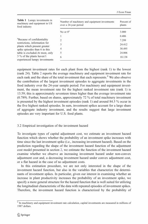
Second, we calculate the number of lumpy investments over a 24-year period andthe percentage of plants with lumpy investments in the industry. Table 1 demonstratesthat over the sample period, 97 % of the plants encounter between 1 and 6 machineryinvestment spikes8 and, at most, only 3 % of the plants haven’t experienced lumpyinvestments.

Third, to investigate both the degree of lumpiness in more detail and the impor-tance of these lumpy episodes in aggregate investment, similar to the studies Domsand Dunne (1998) and Nilsen and Schiantarelli (2003), we rank the machinery and

7 Median investment rate is calculated for each plant using plant observations over the period 1972–1995.We also explored other lumpy investment definitions and didn’t find strikingly different results across thedefinitions.8 Because of confidentiality restrictions, information for plants which present greater spike episodes than 6in this table is excluded. See Geylani and Stefanou (2012) for more detail presentation of lumpiness in theindustry.

J Econ Finan

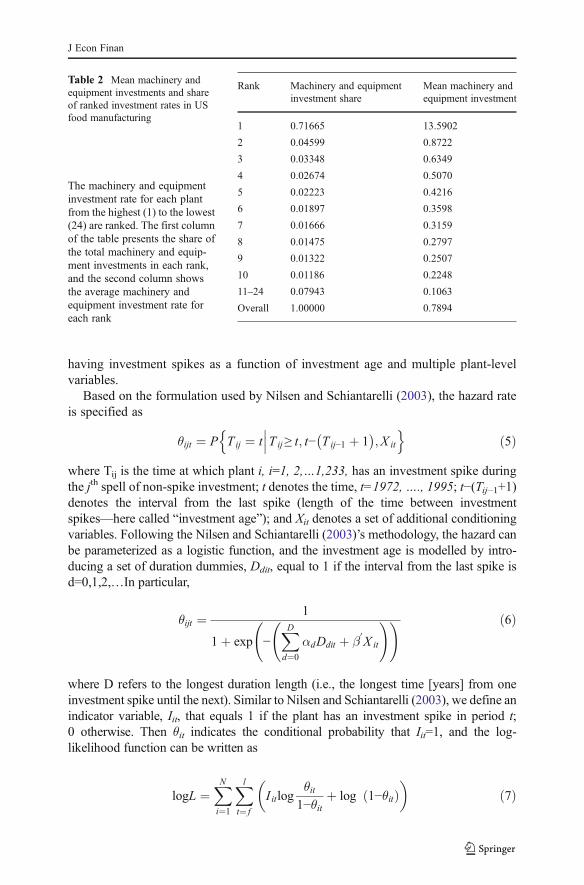
equipment investment rates for each plant from the highest (rank 1) to the lowest(rank 24). Table 2 reports the average machinery and equipment investment rate foreach rank and the share of the total investment that each represents.9 We also observethe contribution of the largest investment episodes to aggregate investments in thefood industry over the 24-year sample period. For machinery and equipment invest-ment, the mean investment rate for the highest ranked investment rate (rank 1) is13.59; this is approximately seventeen times higher than the average investment rate(0.789). Further, based on shares, approximately 72 % of total machinery investmentis presented by the highest investment episodes (rank 1) and around 84.5 % occur inthe five highest ranked episodes. In sum, investment spikes account for a large shareof aggregate industry investment, and the results suggest that large investmentepisodes are very important for U.S. food plants.

3.2 Empirical investigation of the investment hazard

To investigate types of capital adjustment cost, we estimate an investment hazardfunction which shows whether the probability of an investment spike increases withtime since the last investment spike (i.e., increasing investment hazard). Based on theprediction regarding the shape of the investment hazard function of the adjustmentcost model presented in section 2, we estimate the function of the investment hazardexamine whether we observe an increasing investment hazard under non-convexadjustment cost and, a decreasing investment hazard under convex adjustment cost,or a flat hazard in the case of no adjustment costs.

In this estimation procedure, we are not only interested in the shape of theinvestment hazard function, but also in the variables that characterize the determi-nants of investment spikes. In particular, given our interest in examining whether anincrease in plant productivity increases the probability of an investment spike, wespecify a more general structure for the hazard function that is well suited for utilizingthe longitudinal characteristic of the data with repeated episodes of investment spikes.Therefore, the investment hazard function is characterized by the probability of

9 In machinery and equipment investment rate calculation, capital investments are measured in millions of1987 dollars.

Table 1 Lumpy investments inmachinery and equipment in USfood industry

aBecause of confidentialityrestrictions, information forplants which present greaterspike episodes than 6 in thistable is excluded.At most, only3 % of the plants haven’texperienced lumpy investments

Number of machinery and equipment investmentsover a 24-year period

Percent ofplants

No or 0a 3.000

1 0.406

2 7.299

3 24.412

4 30.495

5 24.006

6 10.138

J Econ Finan

having investment spikes as a function of investment age and multiple plant-levelvariables.

Based on the formulation used by Nilsen and Schiantarelli (2003), the hazard rateis specified as

θijt ¼ P Tij ¼ t��Tij≥ t; t− Tij−1 þ 1

� �;X it

n oð5Þ

where Tij is the time at which plant i, i=1, 2,…1,233, has an investment spike duringthe jth spell of non-spike investment; t denotes the time, t=1972,…., 1995; t−(Tij−1+1)denotes the interval from the last spike (length of the time between investmentspikes—here called “investment age”); and Xit denotes a set of additional conditioningvariables. Following the Nilsen and Schiantarelli (2003)’s methodology, the hazard canbe parameterized as a logistic function, and the investment age is modelled by intro-ducing a set of duration dummies, Ddit, equal to 1 if the interval from the last spike isd=0,1,2,…In particular,

θijt ¼ 1

1þ exp −XDd¼0

αdDdit þ β0X it

! ! ð6Þ

where D refers to the longest duration length (i.e., the longest time [years] from oneinvestment spike until the next). Similar to Nilsen and Schiantarelli (2003), we define anindicator variable, Iit, that equals 1 if the plant has an investment spike in period t;0 otherwise. Then θit indicates the conditional probability that Iit=1, and the log-likelihood function can be written as

logL ¼XNi¼1

Xlt¼ f

I itlogθit

1−θitþ log 1−θitð Þ

ð7Þ

Table 2 Mean machinery andequipment investments and shareof ranked investment rates in USfood manufacturing

The machinery and equipmentinvestment rate for each plantfrom the highest (1) to the lowest(24) are ranked. The first columnof the table presents the share ofthe total machinery and equip-ment investments in each rank,and the second column showsthe average machinery andequipment investment rate foreach rank

Rank Machinery and equipmentinvestment share

Mean machinery andequipment investment

1 0.71665 13.5902

2 0.04599 0.8722

3 0.03348 0.6349

4 0.02674 0.5070

5 0.02223 0.4216

6 0.01897 0.3598

7 0.01666 0.3159

8 0.01475 0.2797

9 0.01322 0.2507

10 0.01186 0.2248

11–24 0.07943 0.1063

Overall 1.00000 0.7894

J Econ Finan

where f and l refer the first and last year of plant i’s observations that are used forestimation. Therefore, this form of the log-likelihood can be estimated by using thelogistic estimation as follows:

Pr I i;t� � ¼ Λ β0 þ β1X i;t þ β2TFPi;t−t

� � ð8Þwhere Ii,t=1 if a plant has an investment spike in that year; otherwise Ii,t=0. Xi,t is avector set of relevant plant-level characteristics: dummies for a plant’s lagged invest-ment age, plant’s size, age, 4-digit SIC industry (4-digit output composition), andlagged productivity growth. The inclusion of these of variables allows us to investigatetheir effects on the plant’s probability of having an investment spike and to controlunobserved heterogeneity in the estimation. The investment age variable measures thetime since the plant’s most recent investment spike. In this specification, the range ofinvestment age dummies (Ddit) is 0 to 9 and more, where 0 denotes consecutive spikes;1 represents a one-year investment spike interval, and so on. For the plant size and theplant age variables, we use two different measures to assess if our estimation resultsare robust across definitions. For the first plant size measure, we create quartile groupsto assign size dummy variables for the plants that are based on plant’s weightedaverage employment over the sample period. For the second plant size measure, weuse a continuous variable which is presented by the total employment for each plant ineach year. Similarly, for the first plant age measure, we use dummy variables thatindicate the number of years a plant existed in the census dataset using three differentcensus categories (i.e., 1963, 1967 and 1972). For the second plant age measure, weuse a continuous variable that measures the difference between the current year of theplant and the first year that the plant existed (i.e., 1963, or 1967 or 1972) in theindustry. The last variable is productivity growth lagged by t periods, TFPi, t−t

10 Theproductivity growth is measured at plant level through a Cobb-Douglas productionfunction estimation using Levinsohn and Petrin’s (2003) semi-parametric method. TheLevinsohn and Pertin (2003)’s approach is used to correct simultaneity betweenunobservable productivity and observable input choices. The simultaneity problemoccurs when profit- maximizing firms respond to positive productivity shocks byexpanding output, in turn, using more inputs, creating a simultaneity betweenunobservable productivity and observable input choices (Levinsohn and Petrin2003). This creates bias least squares estimates of production functions which in turnleads to biased productivity estimates.11 As a solution, Levinsohn and Petrin (2003)propose to use an intermediate input (e.g., materials, fuel, or electricity) as a proxycontrolling for the error associated with simultaneity. We estimate the Cobb-Douglasproduction function by using the energy variable as the proxy to control for the error

10 To address any potential endogeneity concerns in our estimation, we use predicted lagged productivityvalues. For the number of periods to lag TFP growth in our regression, we explored various options (e.g.,1st, 2nd and 3rd lagged value of predicted TFP growth; and, 2-year, 3-year (centred on t-2), and 4-yearmoving averages).11 Olley and Pakes (1996) present a solution to this problem by using investment as a proxy variable inestimation to control for the correlated error and the inputs. However, there have been some issues relatedwith investment as a proxy in estimation, in particular micro-level data. For example, an investment proxyis only valid for plants reporting non-zero investment, however, at the plant-level one can observe manyzero investments. Also, non-convexities in adjustment costs may lead the non-responses in investment tosome productivity shocks.

J Econ Finan

associated with simultaneity. The coefficients from this estimation are then used togenerate a productivity growth variable for each plant in each year to be used in ourhazard function estimation in Eq. (8).12 Table 3 gives a description and statistics of thevariables used in the models.

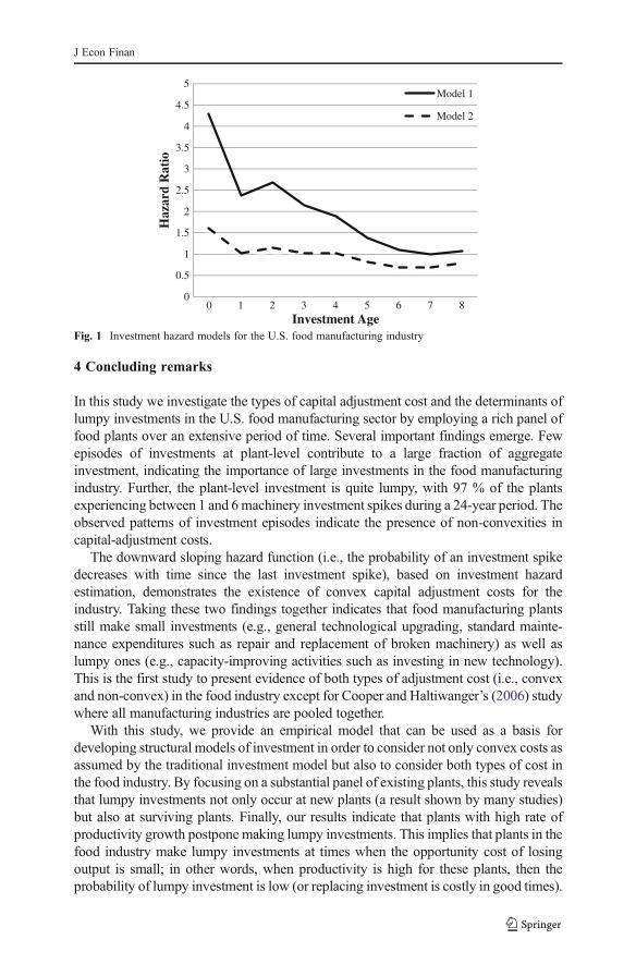
We estimated two hazard models with different plant age and size specifications(Eq. (8)). The estimation results of the hazard models are reported in Table 4. The firstset of results reported in Table 4 (model 1) presents the estimates obtained from thelogit model which uses the dummy representation of the plant size and age variables.Coefficient estimates for the investment age in this model are all positive andsignificant for the first five years. The second set of results reported in Table 4 (model2) presents the estimates obtained from the logit model which uses the plant size andage as continuous variables. Coefficient estimates for the investment age variablefrom this model are positive for the first four investment age variables, on the otherhand, negative and significant for the rest of the coefficients. Figure 1 presents a plotof the hazard ratios using the results from Table 4 (models 1 and 2).13 The generaltrend indicates that the likelihood of having an investment spike decreases sharplyafter the current investment is made, and then declines gradually for subsequent ages.This may be a result of the rapid obsolescence rate in the food industry which causesthe plants to make frequent investments.

In both models, we observe downward sloping hazard function (i.e., negative durationdependence). The downward sloping hazard function (i.e., the probability of an invest-ment spike decreases with time since the last investment spike) indicates that, when aninvestment spike is not occurring, a plant is likely making small investments.14 Thisfinding is a clear evidence of the hypothesis that under the convex adjustment cost, firmsmay change capital stocks to respond optimally to profitability shocks. The theoreticalmodels (e.g., Cooper et al. 1999; Cooper and Haltiwanger 2006) which investigate theeffect of profitability shocks on the shape of hazard function under different adjustmentscost structures predict a negative duration dependence (i.e., decreasing hazard function)under the convex adjustment costs with serially correlated shocks. Our empirical resultssupport this behaviour in such a way that food plants make frequent investments inresponse to profitability shocks under the convex adjustment cost structure. This can alsoindicate that producers invest in capital when there is a capital shortage. Particularly, U.S.food plants may make small investments in order to maintain their competitive positionsin the market and to improve food safety and quality assurance processes that aremandated by regulatory acts.

Nilsen and Schiantarelli (2003) also find that small investment rates are fairlyfrequent and quantitatively important in Norwegian manufacturing plants. Mostrecently, the presence of a mixed form of adjustment costs (convex and non-convex) is explored in a structural model of adjustment by Cooper and Haltiwanger(2006). Their results suggest that a model incorporating both types of adjustment costbest fits the data.

12 The details of the productivity measurement and the coefficient estimates from both the least squares andthe LP approaches are described in Geylani and Stefanou (2012).13 The hazard ratios [Exp (investment age coefficients)] are calculated using the estimated coefficients fromTable 4.14 To check robustness, we estimated the hazard function for major sub-industries in food industry and stillfound a decreasing hazard function even though we controlled for unobserved heterogeneity across plants.

J Econ Finan

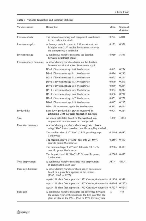
Table 3 Variable description and summary statistics

Variable names Description Mean Standarddeviation

Investment rate The ratio of machinery and equipment investmentsto the real capital stock

0.772 6.011

Investment spike A dummy variable equals to 1 if investment rateis higher than 2.5* median investment rate overthe time period; 0 otherwise

0.173 0.378

Investment age A continuous variable measures the durationbetween investment spikes

6.910 5.530

Investment age dummies A set of dummy variables based on the durationbetween investment spikes (investment age):

D0=1 if investment age is 0; 0 otherwise 0.082 0.274









D9+=1 if investment age is 9+; 0 otherwise 0.313 0.464

Productivity Plant-level productivity growth measured byestimating Cobb-Douglas production function

0.004 0.214

Size An index calculated based on the weighted totalemployment measure over the time period

10088 10657

Plant size dummies A set of dummy variables which assign size classesusing “Size” index based on quartile sampling method:

The smallest size=1 if “Size” <25 % quartile group,0 otherwise

0.2480 0.432

The medium size=1 if “Size” falls into 25–50 %quartile group, 0 otherwise

0.2501 0.433

The medium-large=1 if “Size” falls into 50–75 %quartile group, 0 otherwise

0.2506 0.433

The largest size=1 if “Size” >75 % quartile group,0 otherwise.

0.2505 0.433

Total employment A continuous variable measures total employmentin each plant in each year

387.4 440.41

Plant age dummies A set of dummy variables which assign age classesbased on a plant first appears in the Census(1963, 1967 or 1972):

Age0=1 if plant first appears in 1972 Census; 0 otherwise 0.1420 0.3491



Plant age A continuous variable measures the difference betweenthe current year of the plant and the first year that theplant existed in the 1963, 1967 or 1972 Census years.

19 7.48

J Econ Finan

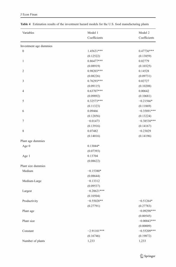
Table 4 Estimation results of the investment hazard models for the U.S. food manufacturing plants

Variables Model 1 Model 2

Coefficients Coefficients

Investment age dummies

0 1.45631*** 0.47736***

(0.12522) (0.13859)

1 0.86477*** 0.02779

(0.08919) (0.10325)

2 0.98203*** 0.14528

(0.08226) (0.09731)

3 0.76293*** 0.02727

(0.09115) (0.10208)

4 0.63707*** 0.00642

(0.09892) (0.10681)

5 0.32573*** −0.21566*(0.11323) (0.11869)

6 0.09466 −0.35891***(0.12856) (0.13224)

7 −0.01473 −0.38538***(0.13916) (0.14167)

8 0.07482 −0.23029(0.14016) (0.14196)

Plant age dummies

Age 0 0.13044*

(0.07393)

Age 1 0.13704

(0.08622)

Plant size dummies

Medium −0.15380*(0.08644)

Medium-Large −0.13312(0.09537)

Largest −0.28621***(0.10504)

Productivity −0.55028** −0.51264*(0.27791) (0.27783)

Plant age −0.09298***(0.00545)

Plant size −0.00043***(0.00009)

Constant −2.91101*** −0.55209***(0.16746) (0.19872)

Number of plants 1,233 1,233

J Econ Finan

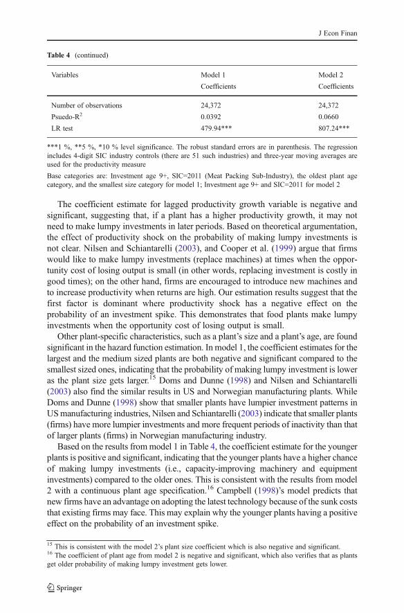
The coefficient estimate for lagged productivity growth variable is negative andsignificant, suggesting that, if a plant has a higher productivity growth, it may notneed to make lumpy investments in later periods. Based on theoretical argumentation,the effect of productivity shock on the probability of making lumpy investments isnot clear. Nilsen and Schiantarelli (2003), and Cooper et al. (1999) argue that firmswould like to make lumpy investments (replace machines) at times when the oppor-tunity cost of losing output is small (in other words, replacing investment is costly ingood times); on the other hand, firms are encouraged to introduce new machines andto increase productivity when returns are high. Our estimation results suggest that thefirst factor is dominant where productivity shock has a negative effect on theprobability of an investment spike. This demonstrates that food plants make lumpyinvestments when the opportunity cost of losing output is small.

Other plant-specific characteristics, such as a plant’s size and a plant’s age, are foundsignificant in the hazard function estimation. In model 1, the coefficient estimates for thelargest and the medium sized plants are both negative and significant compared to thesmallest sized ones, indicating that the probability of making lumpy investment is loweras the plant size gets larger.15 Doms and Dunne (1998) and Nilsen and Schiantarelli(2003) also find the similar results in US and Norwegian manufacturing plants. WhileDoms and Dunne (1998) show that smaller plants have lumpier investment patterns inUSmanufacturing industries, Nilsen and Schiantarelli (2003) indicate that smaller plants(firms) have more lumpier investments and more frequent periods of inactivity than thatof larger plants (firms) in Norwegian manufacturing industry.

Based on the results frommodel 1 in Table 4, the coefficient estimate for the youngerplants is positive and significant, indicating that the younger plants have a higher chanceof making lumpy investments (i.e., capacity-improving machinery and equipmentinvestments) compared to the older ones. This is consistent with the results from model2 with a continuous plant age specification.16 Campbell (1998)’s model predicts thatnew firms have an advantage on adopting the latest technology because of the sunk coststhat existing firms may face. This may explain why the younger plants having a positiveeffect on the probability of an investment spike.

15 This is consistent with the model 2’s plant size coefficient which is also negative and significant.16 The coefficient of plant age from model 2 is negative and significant, which also verifies that as plantsget older probability of making lumpy investment gets lower.

Table 4 (continued)

Variables Model 1 Model 2

Coefficients Coefficients

Number of observations 24,372 24,372

Psuedo-R2 0.0392 0.0660

LR test 479.94*** 807.24***

***1 %, **5 %, *10 % level significance. The robust standard errors are in parenthesis. The regressionincludes 4-digit SIC industry controls (there are 51 such industries) and three-year moving averages areused for the productivity measure

Base categories are: Investment age 9+, SIC=2011 (Meat Packing Sub-Industry), the oldest plant agecategory, and the smallest size category for model 1; Investment age 9+ and SIC=2011 for model 2

J Econ Finan

4 Concluding remarks

In this study we investigate the types of capital adjustment cost and the determinants oflumpy investments in the U.S. food manufacturing sector by employing a rich panel offood plants over an extensive period of time. Several important findings emerge. Fewepisodes of investments at plant-level contribute to a large fraction of aggregateinvestment, indicating the importance of large investments in the food manufacturingindustry. Further, the plant-level investment is quite lumpy, with 97 % of the plantsexperiencing between 1 and 6machinery investment spikes during a 24-year period. Theobserved patterns of investment episodes indicate the presence of non-convexities incapital-adjustment costs.

The downward sloping hazard function (i.e., the probability of an investment spikedecreases with time since the last investment spike), based on investment hazardestimation, demonstrates the existence of convex capital adjustment costs for theindustry. Taking these two findings together indicates that food manufacturing plantsstill make small investments (e.g., general technological upgrading, standard mainte-nance expenditures such as repair and replacement of broken machinery) as well aslumpy ones (e.g., capacity-improving activities such as investing in new technology).This is the first study to present evidence of both types of adjustment cost (i.e., convexand non-convex) in the food industry except for Cooper and Haltiwanger’s (2006) studywhere all manufacturing industries are pooled together.

With this study, we provide an empirical model that can be used as a basis fordeveloping structural models of investment in order to consider not only convex costs asassumed by the traditional investment model but also to consider both types of cost inthe food industry. By focusing on a substantial panel of existing plants, this study revealsthat lumpy investments not only occur at new plants (a result shown by many studies)but also at surviving plants. Finally, our results indicate that plants with high rate ofproductivity growth postpone making lumpy investments. This implies that plants in thefood industry make lumpy investments at times when the opportunity cost of losingoutput is small; in other words, when productivity is high for these plants, then theprobability of lumpy investment is low (or replacing investment is costly in good times).

0

0.5

1

1.5

2

2.5

3

3.5

4

4.5

5

0 1 2 3 4 5 6 7 8

Haz

ard

Rat

io

Investment Age

Model 1

Model 2

Fig. 1 Investment hazard models for the U.S. food manufacturing industry

J Econ Finan

There are possible policy implications that can be derived from the empiricalresults of this study. The adjustment cost structure of a firm is an important factor inunderstanding a firm’s input demands and productivity, as well as, in predicting theimpact of factor market policies on the aggregate level. Thus, in order to investigatethese effects accurately, we need to incorporate plant-level information (e.g., invest-ment and cost structure at the most micro level) into our analysis. Some of the resultsfrom this study may inform policy makers to observe firm behaviour towards theirpolicies (such as investment tax credits that are geared towards encouraging invest-ments) that are offered for them. For example, the evidence of non-convex adjustmentcost can inform policy makers why some firms may not take advantage of tax creditsthat encourages continuous investment in new capital.17

Future research can benefit from a structural model that allows us to formalize aricher model of adjustment costs (containing both types). Further, we can formallycompare the predictions of the effects of a factor market policy at plant-level and ataggregate level from a model which considers traditional convex adjustment cost withone that considers a more complex form of adjustment cost alternatives.

Acknowledgments I would like to thank three unanimous referees for their valuable suggestions andcomments. The research in this paper was conducted while the author was a special sworn status researcherof the U.S. Census Bureau at the Michigan Census Research Data Center. Any opinions and conclusionsexpressed herein are those of the author and do not necessarily represent the views of the U.S. CensusBureau. All results have been reviewed to ensure that no confidential information is disclosed. Supports forthis research from the U.S. Department of Agriculture/National Research Initiative (award no. 03-35400-12949) and at the University of Michigan RDC from NSF (ITR-0427889) are gratefully acknowledged.

References

Abel A, Eberly J (1994) A unified model of investment under uncertainty. Am Econ Rev 84(5):1369–1384Abel A, Eberly J (1996) Optimal investment with costly irreversibility. Rev Econ Stud 63(4):581–593Bertola G, Caballero R (1994) Irreversibilities and aggregate investment. Rev Econ Stud 61(2):223–246Caballero R, Engle E (1999) Explaining investment dynamics in U.S. Manufacturing: a generalized (S,s)

approach. Econometrica 67(4):783–826Caballero R, Engle E, Haltiwanger JC (1995) Plant-level adjustment and aggregate investment dynamics.

Brookings Pap Econ Act 2:1–39Campbell J (1998) Entry, exit, embodies technology, and business cycles. Rev Econ Dyn 1(2):371–408Carlsson M, Laseen S (2005) Capital adjustment patterns in Swedish manufacturing firms: what model do

they suggest? Econ J 115:969–986Cooper R, Haltiwanger JC (2006) On the nature of capital adjustment costs. Rev Econ Stud 73:611–633Cooper R, Haltiwanger JC, Power L (1999) Machine replacement and the business cycle: lumps and

bumps. Am Econ Rev 89(4):921–946Dixit AK, Pindyck RS (1994) Investment under uncertainty. Princeton University Press, Princeton, New

JerseyDoms M, Dunne T (1998) Capital adjustment patterns in manufacturing plants. Rev Econ Dyn 1:409–429Dunne T, Mu X (2010) Investment spikes and uncertainty in the petroleum refining industry. J Ind Econ

58(1):190–213Gelos RG, Isgut A (2001) Fixed capital adjustment: is Latin America different? Rev Econ Stat 83(4):717–726Geylani CP, Stefanou ES (2012) Linking investment spikes and productivity growth. Empir Econ.

doi:10.1007/s00181-012-0599-8

17 We would like to thank an anonymous referee for suggesting this point.

J Econ Finan

http://dx.doi.org/10.1007/s00181-012-0599-8

Goolsbee A, Gross DB (1997) Estimating the form of adjustment costs with data on heterogeneous capitalgoods NBER working paper no. 6342

Hamermesh SD, Pfann GA (1996) Adjustment costs in factor demand. J Econ Lit 34(3):1264–1292Letterie WA, Pfann GA, Polder JM (2004) Factor adjustment spikes and interrelation: an empirical

investigation. Econ Lett 85:145–150Levinsohn J, Petrin A (2003) Estimating production functions using inputs to control for unobservables.

Rev Econ Stud 70(2, 243):317–342Nilsen OA, Schiantarelli F (2003) Zeros and lumps in investment: empirical evidence on irreversibility and

nonconvexities. Rev Econ Stat 85(4):1021–1037Olley GS, Pakes A (1996) The dynamics of productivity in the telecommunication equipment industry.

Econometrica 64(6):1263–1297Power L (1998) The missing link: technology, investment, and productivity. Rev Econ Stat 80(2):300–313

J Econ Finan

lumpy investments and capital adjustment patterns in the food manufacturing industry

Documents