lp sobolev spaces - tsinghua...
TRANSCRIPT

Acta Math., 171 (1993), 165-229
A global calculus of parameter-dependent pseudodifferential
boundary problems in Lp Sobolev spaces
by
GERD GRUBB and NIELS JORGEN KOKHOLM
University o] Copenhagen Copenhagen, Denmark
University of Copenhagen Copenhagen, Denmark
In tro d u c t io n
The theory of pseudodifferentiai boundary problems has been developed to provide a
larger framework for the study of differential boundary value problems, allowing algebraic
manipulations with the operators (reflected in a symbolic calculus) and allowing the
inclusion of non-local terms. The elliptic calculus has its origin in works of Vishik, l~skin
and Boutet de Monvel (cf. [V-E], [E], [BM1] and in particular the Acta article [BM2])
and was further developed e.g. in Rempel and Schulze [R-S1] and Grubb [G1]. The scope
of the theory was enlarged by the consideration of systems depending on a parameter
(running in a noncompact set), which can be for example a spectral parameter )~E(~
(allowing functional calculus), a time dependence (for parabolic problems) or a small
parameter c >0 (entering in singular perturbation problems). For operators in L2 spaces,
such a theory was worked out in the book [G2], and further developed for parabolic
problems by Grubb and Solonnikov [G-S1], who applied it to give new results on fully
nonhomogeneous Navier-Stokes problems (cf. [G-S2] and its references). Let us also
mention the treatment in [R-S2] of resolvent estimates and complex powers for systems
without the so-called transmission property.
The purpose of the present work is to extend the parameter-dependent calculus
to the Lp setting, 1<p<cr and to a suitable class of unbounded manifolds, including
exterior domains (complements of smooth compact sets) in R n and ~n +.
A fundamental difficulty in the study of parameter-dependent elliptic pseudodiffe-
rential problems, depending e.g. on a spectral parameter A on a ray in C, is the following:
Without the parameter, the singularity of the homogeneous symbols at ~=0 is harmless
(since it is felt in a compact set only), but when A is adjoined, the singularity has an

166 G. G R U B B A N D N. J . K O K H O L M
important influence as I)~1--*oc. This is reflected in a complicated structure of the symbol
classes, noticeable already for the pseudodifferential operators P in the theory, but even
more so for the boundary terms (the trace operators T, Poisson operators K, singular
Green operators G).
The book [G2] handles this problem by introducing a version of the Boutet de Monvel
calculus with symbols depending on a parameter # ( a suitable power of }~), where It has
much the same role as the cotangent variables in the ps.d.o, calculus, but enters with less
regular estimates. The symbol seminorms for operators on R~ are formulated by use of
L2(R+) estimates, where x,~ ER+ is the variable normal to the boundary (here one finds
that e.g. systems of supremum norms, that are equivalent with the present choice in the
non-parametrized case, are far from equally efficient when the parameter is included);
and the full calculus is established in this framework. L2 Sobolev space estimates of the
operators are obtained by use of convenient properties of the Fourier transform.
For Lp results one might expect that it would be necessary to work the symbolic
calculus over again with Lp(R+) estimates, but we found that this is neither necessary nor
very useful. In fact, the results can very well be obtained on the basis of the development
in [G2]. Mapping properties in Lp(R~) Sobolev spaces are obtained by use of multiplier
theorems of Mihlin and Lizorkin with respect to the tangential variable x', valued in
Hilbert spaces of functions of xn. (The theorems do not hold generally in Banach spaces,
which is why Lp(R+) symbol estimates are not used.) Our point here is that we can
get the desired Lp(R~_) estimates on the basis of certain weighted L2(R+) and H~(R+)
estimates derived from the calculus of [G2], by use of an interpolation result from Gilbert
[Gi] together with other results on Bessel-potential and Besov spaces (cf. [T1]).
In the process, we have revised the results of [G2] and worked out some precisions
of that calculus; notably, a certain "loss of regularity" occurring there has been almost
eliminated. We have also found a simplification in the use of "order-reducing operators",
namely that the simple version ( ( D ' I • t composes in a very good way with the
boundary operator types K, T and G, and hence can be used in many places where one
would think it necessary to use the more refined version of [BM2]. Moreover, we extend
the calculus to unbounded manifolds with finitely many conical ends, by working with a
special type of symbols that are uniformly estimated in x (as in HSrmander [H3, 18.1] for
ps.d.o.s without p-dependence); and systems of negative class are included (generalizing
[G3]). - - Some of our results were announced in [G-K].
Contents. Section 1 introduces the appropriate Bessel-potential spaces H~,t'(~) and
Besov spaces Bp,~(~) depending on a parameter I tER+; and the expected properties
(interpolation, duality, imbedding and trace theorems) are established, uniformly in the
parameter. The admissible unbounded manifolds are defined. The needed variable-

A GLOBAL CALCULUS 167
coefficient version of Mihlin's and Lizorkin's theorems is presented, and we show some
particular interpolation results to be used later.
In Section 2, we introduce a stricter, globally estimated version of the symbol classes
in [G2], based on [H3, 18.1] (results for symbol classes with local estimates can be re-
covered from this). An advantage of the global calculus (besides allowing unbounded
manifolds) is that it gives more precise results: the so-called negligible operators are
included in the operator spaces instead of forming residual classes, and the compositions
and inverses on R~_ (when they exist) are defined by precise symbols in the calculus.
In Section 3, we show how a certain projection estimate from [G2] can be sharpened,
allowing any E > 0 instead of ~= �89 for (0,2) below. We introduce negative classes and study
the composition of boundary operators with operators ((D'> +iDn) t, and we prove some
delicate estimates of the boundary symbol operators in weighted L2 spaces, crucial for
the later Lp estimates.
In Section 4, we prove the main theorem on continuity in Hi '" and B~'" spaces. It
is found, roughly speaking, that for boundary operators of regularity u, the continuity
holds with an 0((#> -~+11/2-1/pl +1) estimate of the operator norm, and for ps.d.o.s it
holds with an O((#)-~+1) estimate (see the precise statements in Theorem 4.1 below;
for the necessity, see Remark 4.2). In particular, if u~> �89 the estimates are uniform in #
for each pE ]1, ec[.
Finally, Section 5 gives the full proof of composition rules for the present operator
classes, showing that when ~4~ and ~4~ are Green operators of order d resp. d', class r
resp. r' and regularity u resp. u !,
(P. ++c. A. \ 'T. S. ' A =k
(0.1)
then (when the matrix dimensions match) A,.A~ is again a Green operator:
! I l l l! \ ( P" -L(P,,P;)+G, K~ (0.2) zl I! A fl[! _~ ",+ ) " ' . = " . T# S; '
of order d'=d+s and class r"=max{r',r+d'}, with all terms of regularity S -
rain(u, u', , + u ' ) except L(P,, P~), that is of regularity u"-E, any E>0.
Applications. The above gives the fundamental steps necessary for establishing the
calculus in the desired generality. In sequels [Gh] to this paper, polyhomogeneous
parameter-elliptic Green operators ,4, are considered; it is shown that parameter-eUiptic
operators are invertible (within the calculus) for sufficiently large #, and that an inverse,
when it exists, belongs to the calculus; and the consequences for parabolic pseudodifferen-
tial boundary problems (in anisotropic Bessel-potential and Besov spaces) are developed.

168 G. G R U B B AND N. J. K O K H O L M
Moreover, a concrete application of the anisotropic Lp Sobolev space results to the time-
dependent nonhomogeneous Navier-Stokes problem along the lines of [G-S2] is worked
out. Further consequences for Navier-Stokes problems with initial data of low regularity
have been derived in [G6].
1. Spaces and manifolds
1.1. Besse l -potent ia l and Besov spaces wi th a parameter
There are many good explanations of the various generalizations of Sobolev spaces in
the Lp situation, cf. e.g. Stein [St], NikolskiY [Nil, Bergh-L6fstr6m [B-L], Triebel [T1,2].
In the present paper we shall use the terminology summed up in [G3] (based to a large
extent on IT1]), without repeating the full details here, where we shall focus on the
information on parameter-dependent spaces necessary for our presentation.
Let l < p < c ~ . We recall that a constant-coefficient pseudodifferential operator Q
with symbol q(~),
Qu = OP(q(~))u = q(D)u = .~u-1 (q.~?A)
(where ~" is the Fourier transform), is continuous in Lp, if one of the following criteria
(derived from the Marcinkiewics multiplier theorem) holds:
C(q)- sup lSIl~llD~q(5)l < oo (Mihlin [M]),
C'(q)- sup ]~"n~q(~)] < c~ (Lizorkin [L]); a l =0,1 , ~ E R ~
(1.1)
and the norm is ~CpC(q) resp. CpC'(q), where Cp is independent of q. Lizorkin's
criterion covers a different type of symbols than Mihlin's, since "mixed" expressions
~iD~q with i ~ j do not enter. (The total order is higher there, when n>~3, but in many
situations that is no problem.)
In order to state estimates of parameter-dependent Green operators in Bessel-
potential (Hi) and Besov (B~) spaces, we introduce for each of these spaces a family
of equivalent norms depending on a parameter #. The parametrized norms are intro-
duced first for spaces over R n, then for spaces over R~_ = {x E Rnlxn >10}, and finally for
spaces over suitable manifolds with boundary.
Consider first the spaces over a n. Let {~)=(1+1~12) 1/2, and denote OP((~)s)= {D) s. Recall that the Bessel-potential space H~(R n) is defined as the space of f E S ' ( R n) for
which (D)Sfeip(R"), with norm
[IfllH~(P,.,~) = [[(D)*fIIL,,(Rn) �9 (1.2)

A GLOBAL CALCULUS 169
For s eN, H~(R ~) equals the Sobolev space Wp(R n) that consists of the functions f
with D~f e Lp(R '~) for l al ~< s. For s e R+\N, another definition is used for the Sobolev-
SlobodetskiY space W~(Rn); it is taken equal to the Besov space B~(Rn). Here B~(R ~)
can be described either in terms of an integral formula:
for se]0,1[, : e B ~ ( R ~) ~-~ II/IIL,+fR I:(x)-:(Y)IP dxdy<c~, ~ Ix-y l ~+p" (1.3)
fors, t e R , ,+t n t , n . feB,, (R) ~-~ (D) feB~(R ),
or in terms of a norm defined by a partition of unity as follows (cf. e.g. [B-L, Lemma
6.1.7]): Let ~ e C ~ ( R n) have the properties
supp~={~12-1 ~< I~1 ~<2},
~ ( r when 2 -1<[r
E ~ ( 2 - k ~ ) = l when[~l~0,
and define ~0eC~(R ~) by
~ o ( ~ ) = 1 - E qa(2-k~)" l~<k<c~
Then Bp(Rn)=B~,p(Rn), where, for any s e R and 0<q<c~, the space B;,q(R n) is de-
fined as the space of tempered distributions f with finite norm
/ IIflIB:~,~(R~) : ~,ll~oo(D)fllq,(R~)+
IIflIB:,(R~) = llfllB:o,,(R~)"
(2"kll~(2-kD)fllLPfW~))q) 1/q; (1.4) l~<k<c~
Parameter-dependent versions are now defined as follows: Let #ER.+ (we could
equally well let #ER). For the Bessel-potential spaces, we simply take the norms
IIfIIHg''(R~)=I[(D,#)'fIIL~(R-), where (D, #)s = OP((r #) ' ) = Z~, (r #) = (1+ Ir +~2)x/2 (1.5)
(Also (2.2) or (2.3) can be used.) For each fixed #, this is equivalent to II:llH$(a-), by Mih- lin's criterion (the functions (r162 #)-1 and (r #)(r satisfy (1.1)), but with estimates
depending on /z. For s>~0, the functions (~,/z) ' /((r s) and ((~)s+(#)~)/(r
satisfy Mihlin's criterion with constants independent of #, so
/l:ll.;,.(a~) = II <D, #)'fIIL.(R~) = II 0P((r #)'/((r + (#)')) 0P((~c)" + </~>~):II Lto(R n)
<. CI(II(D)" flIL,(Rn) +(IZ)'IIflIL,(R,~));
170 G. G R U B B A N D N. J . K O K H O L M
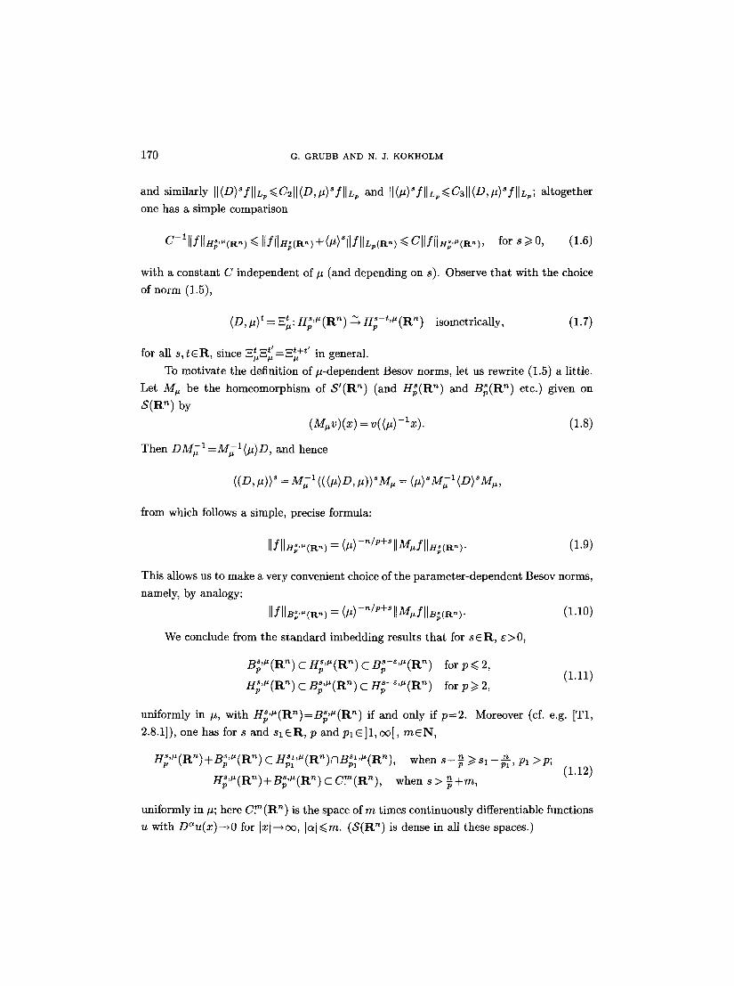
and similarly ]]<D)~f[[L~ ~<C2[[(D,/Z>~fIIL~ and I{</Z>*fIIL~ ~C3[I<D,/Z)~fIIL.; altogether one has a simple comparison
C-I[[f[[H~,~,(R,,) <~ [[f[[H~(R.,)+(/Z)*[[fI[L,(Ft,,) <<. CI[f[IH;,,(R,,), for s ~> 0, (1.6)
with a constant C independent of/Z (and depending on s). Observe that with the choice
of norm (1.5),
(D,/z)t _-- -z'=t. Hp,U(R.) __% Hp-t,U(R.) isometrically, (1.7)
for all s, t c R , since =t =,' _~,+, ' in general. ~ # ~ I z - - ~ l z
To motivate the definition of/z-dependent Besov norms, let us rewrite (1.5) a little.
Let Mu be the homeomorphism of 8 ' ( R n) (and Hp(R '~) and Bp(R n) etc.) given on S (R n) by
(Uuv)(x) = v((#)-Ix). (1.8)
Then DM~ 1 =M~ 1 (/Z)D, and hence
((D,/Z))~ = Mu -1 (((/Z)D,/Z))~M u = (/Z)~M~ 1 (D)*Mu,
from which follows a simple, precise formula:
[[fllHg'~(R") = </Z>-n/P§ IIMjIIHg(R~)" (1.9)
This allows us to make a very convenient choice of the parameter-dependent Besov norms,
namely, by analogy:
IlfllB;..(~-) = </Z)-~/P+~ IIM.flIB~(~-). (1.10)
We conclude from the standard imbedding results that for s E R, e > 0,
B~'U(R")CHp'U(R'~)CBp-~'U(R "~) f o r p < 2 , (1.11)
H~'U(R'~) C B;'U(R") c H;-~'U(R ") forp~>2,
uniformly in #, with H~'~'(Rn)=B~'U(R n) if and only if p=-2. Moreover (cf. e.g. [T1,
2.8.1]), one has for s and s lER, p and plE] l , oo[, mEN,
Hp'U(gn)§ ~) C Hp~'U(Rn)NBp~'U(R~), when s - p ~> s, - ~ , Pl >P; (1.12)
Hp'U(Rn)§ when s > p §
uniformly in #; here C.m(R n) is the space of m times continuously differentiable functions
u with D~u(x)---~O for txt--~oo, [at~<m. (S(R ~) is dense in all these spaces.)

A GLOBAL CALCULUS 171
Observe also the following difference: For s=0,
II'/IH~ : I['[IL~(R-) for all/z e R§
whereas I[.IIBo,.(R~) depends in an essential way on # when pr In fact, we have for all
f E S ( R n) in view of (1.4) and (1.10),
Ilfll~o,-(R~) ~ IIfIIL~(R~) as lZ ~ ~ , (1.13)
where Lp(Rn)=H~162176 ~) when pr
We need to know that the interpolation, duality and trace theorems valid for the
usual Bessel-potential and Besov spaces have counterparts for these parameter-dependent
spaces, with estimates uniform in ~. The statements and proofs will be straightforward
when we use (1.9) and (1.10). To give an example, recall that real interpolation (-,.)O,p
(cf. [B-L, Theorem 6.2.4]) of the Bessel-potential spaces H~~ ~) and H~I(R ~) with
0<0<1 and so~sl , gives the Besov space B~(R~), where s=(1-0)s0+0Sl . In particular,
for some constant C>0 independent of f we have when fEB~(Rn):
C -1 IlfllB$(~) < Ilfll(HgO (a~),Hgl (R~))~,~,~ < CIIfilBgR~). (1.14)
(The precise value of the interpolation norm depends on the method; here we refer to
the K-method, to fix the ideas.) Since M~, is a homeomorphism in all these spaces,
and the exponent - p + S in (1.9) and (1.10) is an affine function of s, we get with the
same C:
C--111flIBg'~(R ~) ~ IIfI[(H;~ ~ CIIfIIBg'~(R~)"
We formulate this result as follows:
( 1 . 1 5 )
(H~~ H~,l't'(Rn))o,p ~- B~#'(Rn), uniformly in #, with s = (1-0)So+0Sl.
(1.16)
Recall that for f in the smallest of the spaces,
.< 1-0 o (1.17) IIfIIB~,~(R-) -~ CIIflIH;o,.(R~)I{YllHT'"(rt-)"
As an application, we see that for each t, sER,
(D, #)t =_~,._p=t. Rs,~,(Rn~,_ j -% B~-t,~(Rn), uniformly in # (1.18)
(in the sense that the operators (D, p)t and (D, p)- t between these spaces have bounds
independent of/z). Because - 9 +s is affine in ~ too, all the other interpolation and
12- 935204 Acta Mathematica 17 I. Imprim6 le 2 f~vder 1994

172 a . GRUBB AND N. J. KOKHOLM
Lmbedding results of [B-L, 6.2 and 6.4] generalize immediately to/~-uniform results for
the parameter-dependent spaces. The same is true for the duality results, since (.1.10)
menus that (#}-'qP+sMt~ is an isometry of B~'t'(R n) onto B~I(R'), and thus
( ( (U}-,~II,§ M , }* ) - ~ = (#~)nl.-~ (p}-n M~ ̀ = (#j)~IP'-* M ,
is an isometry of B;,~'(Rn) * onto B ; ( R ) =B; , ( R ) , where
; + ~ * = i . ( I ,19)
(The notation {1Lig) ~ be. used throughout.)) Thus for alI sER,
s;,,(R~)*_~ B~""(R~)~ ~ifo, mly in •. (1.20)
Fkl.MIy, we have: for the restriction operator" ~o: u:(x)~-~u(x',O) (from R ~ to R~-I) ,
s ince- -~ : t . - - - T . ~ s - - ~ ) and ~(M~,u)=:M~,'~oU', that the usual trace theorem (cf.
e,g. [EaL, Ttmorem 6.6.I])impEes:
" 7 0 " r r s , , ~ ~ " ~ . r~ "~, - - + r ~ - l / p l* f ' r * r e - l; " ~
(1.21) :0:B;'~(R'~)~--~B~p-i/P"~(R'-:): ~ni$ormIy hi ~ for , > '
mad, eammt ~ . t ~ a -<-: (el:, e.g: [Ga, Lemma 2.2 D. ~ p
C~r g sp~ces de~imc[ relative to R~_, one has the tmuaI two variants. On one
k a ~ there are: the ~ s ~ b s ~ of distributions supported in ~t ~
H~, , , , -~ , _ n;, ,~(l lO)l ~ p i , , c R ~ } ; ,,;~ ( R + ) - {~ e . . . . , (122)
that i n ~ the norm from the fu~ spaces; and on the other hand, there are the distri-
hmion spaces over R ~ obtained by restriction:
H ~ : ' u ~ " = r + n g ' " ( R ~ ) , B; . 'v(R:) =r+B.;'V(R'~); (1.23)
t h w are provided with the in6mum norms
Ulf~;,*(~:)=inf{ llgtl.;,,'(R:)lg~H;'V(Rn), r + g = / } , etc. (1.24)
Here r --e demotes restriction to R~_ (and we later also use e +, extending functions on R~
by zero on R ~ \ l ~ ) . The spaces
8 0 ( R ~ ) = { u e S ( R ' ~ ) [ s u p p u c R . ~ } resp. , 9 ( R ~ ) = r + S ( R ") (1.25)

A GLOBAL CALCULUS 173
are dense in rrH,gr~n-~ and BH'gq~ n ~ resp. H2,U(R~) and ns ,u[~n ~. and the norms in ~ p ; 0 KL~'+] p;0 ~, +1 p U p K - - + / ,
the latter equal the quotient norms when we identify
H s't'(~'~ ~ "~ H s''(~'~lt-r~'~'{~n ~ etc, (1.26) p ~ = ~ + ] ~ p k ~ '~ J / ~ p ; O K ~ ] '
(There is a detailed analysis e.g. in ~ e b e l [T1, 2.8, 2.9] of the spaces in the/z-independent
case; H~;0(R+)~ ~ - n and B sp;o~.r ~ are ca l l ed /~ (R +) resp. Bp,p(R~~S +) there.) Now the crucial
observation is, that since the dilation x ~ (#)x preserves R~, we can conclude that the
norms are related to the gAndependent norms in the same way as for the spaces over Fin:
I[fllX~, = <l.t)-n/P+SllMufi[x~ for s ER, with (1.27)
p;0(a+),/~p(P~) or B~o(n+). Uniform interpolation, imbedding, duality, trace and extension theorems then follow
from the case without a parameter just as above. (For an overview of relevant non-
parametrized statements~ see [G3].) Let us collect some of the resulting statements in a
theorem.
THEOREM 1.1. The following identifications hold, uniformly in #:
(g~ (R+),H~ (R+))o,p-(H;'V(R~),B~'g(R~))o,p
(1.2s) (Z ; (R+),H$ (R+ ))0,v, "
[B; (a+) , p ( r t + ) b _ : ~ , . .+ , ,
[g ; (R+), ~ (R+) ]o - where
s, teR, s#t, p, qZ]l,~r 0s]0,1[, s,=(1-O)s+Ot, $ - ~ + ~ .
Here the dual spaces are defined with respect to an extension of the sesquilinear duality (u,v)R~ =:frt~ u(x)V(x)dx; and the interpolations that are used are real interpolation
( ' , ')o,p resp. complex inte~lat ion [., . ]o. The interpolation statements hold also with Hp and B~ replaced by H~o and B~,;o, and the norms satisfy generalizations of (1.17).
The trace operator q~: u( x ) ~ D~ u( x', O) is continuous for s > j + ~,
I:[s,~,[~n ~a.ns,ut~n ~ ._+ t~,=J~l/~,t'tl~n-~ uniformly in #, (1.29)
Note also that in view of (1.6),
C -~ I[/ll.;,.(a;) 4 lit H;(a~)+(.)" i1 iz.(a~) < 6'll/ll.;,.<a~), for each s ~ O, (1.30)

174 G. GRUBB AND N. J. KOKHOLM
with C independent of #.
For the spaces over R~_, the following operators are more convenient than the =t.
Denoting (~1, .-., ~n-1)=~', we let
x~(~,u)=(<( , . )+i~) t, teR, X~: (~' , . , On) = OPt . (X~=(~, . ) ) = ((~', . ) + i O n ) t, (1.31)
E~=,u = OP(xt, (~, . ) ) -- (<D', .> +iOn)t;
then one has for all t, sER:
(•• (1.32) ~ + , t t ~ • - - ~• - - ~:F,/~"
Moreover, the funtions (~, . )- t((~, , #)+i~n)t satisfy Lizorkin's criterion (1.1) uniformly
in # for each tER, and hence the operators
-u - • = OP(<~, . ) - t ((~,, . ) +i~.~)t)
are bounded in Lp(Rn), uniformly i n . , for any s and t, which implies
"~t . r _ r s , u t ~ n ~ ~ r . g s - t , u t ~ n ~ (1.33) -• "'p ~ J ~ " p ~ j, uniformly i n . ,
with similar statements for B~ ,u spaces. We define as usual
PR?~ =r+Pe +, also written for short as P+.
By the Paley-Wiener theorem, the operators F.~_,u map So(R~) onto itself, and .-t =t'
equals =t+t' there, so by extension by continuity and by duality one gets the homeomor-
phism properties:
THEOREM 1.2. For all s, t E R one has, uniformly i n . ,
~ t . L l " s , ~ ( ~ n ~ _~ l : . 1 s - t , / ~ [ ~ n "~ ,~t ,~s = ~ t + s . ~ + , g " * 'p ;0 k*~+) ~*p;0 t ' ~ + ] , with ~+, lz ,R_~+, /z ,R~_ ~ + , / ~ , R ~ '
(1.34) s ,p - - n ~ 8 - t , ~ - - n ~ t ~ s ~ ~ t + s =t . :Up (R+)--*H; (R+), with ~--,Iz,l:t+ --,t~,R+ --,~,R+ ~-,/~,R~"
(On distribution spaces where e + is not defined, Et_,u,rt~ is taken as the continuous
extension from S(fft~_).) The analogous statements hold with Hp replaced by Bp.
Here the results in Besov spaces follow from the results in Bessel-potential spaces
by interpolation, using (1.28). We note furthermore that the mapping - -~ (")=-,ma~ is p ~ s , ~ l ~ n ~ bounded in ..p ~.~+~ and in B~,~(R~_), uniformly i n . , so that for each s~R,
IlfllH;-~,,,(n.7.) ~< Cs(U)-~ll.fll.~:,,,(n~.), tlfll.g-l,,,(~.7.) ~< C~(.)-lllfll.g,,,(~.~_). (1.35)
We observe the following simple property of the spaces:
A G L O B A L C A L C U L U S 175
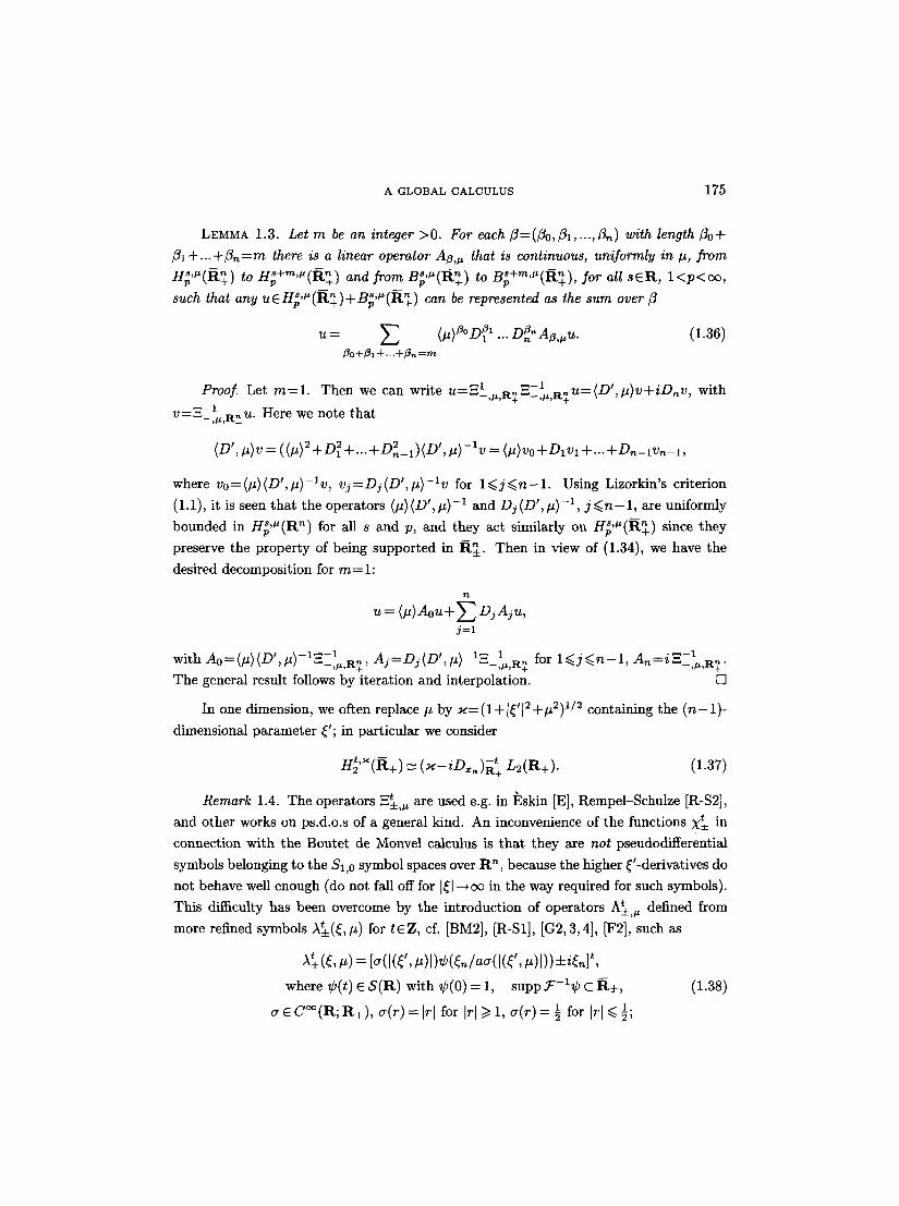
LEMMA 1.3. Let m be an integer >0. For each ]~=(~0,f~l,...,f~n) with length 13o+ ~l+. . .+~n=m there is a linear operator A~,~, that is continuous, uniformly in #, from H~_'~(ft~)~ to ..p~8+'~'~(~n~+~ and from B~,~(R~_) to B~_+m,~(~t~_),~ for all s s 1 <p<co ,
such that any s,~ - n ~,~ --,~ ueH~ (R+)+B~ (R+) can be represented as the sum over Z
u= ~ (#>~~ . . .D~'A~,#u. (1.36) ~o+fh +.. .+~=m
_ ' ' 1 ~ - - 1 t Proof. Let m = l . Then we can write U----_,~,R?=_,~,RrU=(D,#)v+iDnv, with
V==_,~,R?U. Here we note that
I 2 2 2 ! - - i <D ,#)v=((#> +DI+.. .+Dn_I)(D ,#> v= (lZ)vo+DlVl+...+nn-lVn-1,
where vo=(#)(D',#)-lv, v j=Dj(D~,#)- lv for l<.j<.n-1. Using Lizorkin's criterion
D "D p ,-1 j<.n-1 , uniformly (1.1), it is seen that the operators (#)(D~,#) -1 and j / ,#) , are r48,~C~n ~ since they bounded in H~,~(R n) for all s and p, and they act similarly on ..~ ~.~+j
preserve the property of being supported in R~. Then in view of (1.34), we have the
desired decomposition for m--1:
n
u = (#)Aou+~-~ DjAju, j = l
,,\ -I~--I n " ~_ . with Ao = (#)(D', ~ ---,.,R+, Aj =Dj (D', ~)-IE-~.,R ~ for l~<j ~<n-- 1, An =z ---~,R~
The general result follows by iteration and interpolation. []
In one dimension, we often replace # by x=(1+[~'[2+#2) ~/2 containing the (n-1) -
dimensional parameter ~'; in paxticular we consider
g~'~' (ft+ ) ~- ( x - i D ~ )~t+ L2(R+). (1.37)
Remark 1.4. The operators -• are used e.g. in ]~skin [E], Rempel-Schulze [R-S2],
and other works on ps.d.o.s of a general kind. An inconvenience of the functions X~= in
connection with the Boutet de Monvel calculus is that they axe not pseudodifferential
symbols belonging to the S1,0 symbol spaces over R n, because the higher ~-derivatives do
not behave well enough (do not fall off for ]~[--+co in the way required for such symbols).
This difficulty has been overcome by the introduction of operators A t defined from •
more refined symbols A~=(~, #) for fEZ, cf. [BM2], [R-S1], [G2, 3, 4], [F2], such as
.,V, = [o-(I (,f', I)) +i,1,,] where r E 8(R) with r = 1, supp~ ' - l r C R.• (1.38)
a e C~176 a ( r ) = [r[ for ]r[/> 1, a(r)= �89 for ]r] ~< 5,1"

176 G. GRUBB AND N, J. KOKHOLM
and a>0 is taken so large that ar177162 for all values of a and ~ (e.g, a>~
2supt lr These symbols ave truly pseudodifferential, elliptic, of regularity +oc in
the terminology of [G2], and have the transmission property. Moreover, they have the
same mapping properties as the --t listed in (1.34) (fEZ), shown in a similar way, see ~=}:,g
also [G3, Theorem 5.1]. (The hypothesis s u p p ~ ' - l r was not always included, it
assures the extension of the mapping properties as in (1.34) to negative s, cf. IF2], [G3].)
But in fact we shall show below in Section 2 that the operators in (1.34) are, after
all, useful in the Sl,o pseudodifferential boundary operator calculus, as long as they are
only composed with the "singular" operators, i.e. with Poisson, trace and singular Green
operators, where they do preserve the operator classes. This observation will allow us to
make some calculations in a simpler way than if the A~= were to be used. We shall even
discuss some estimates where noninteger powers t are involved. (When t~ Z, neither the
A~: nor the X~ have the two-sided transmission property that plays an essential role in
the Boutet de Monvel calculus, so they are rarely considered then.)
1.2. Admiss ib le manifolds
Now let us say a few words about corresponding spaces defined over more general subsets
of R n and manifolds. Here we shall use the following two fundamental observations:
(i) When CEC~ n) is bounded and all its derivatives are bounded, the mapping f~-~r is continuous from H~'~(R '~) resp. B~,#(Rn) to itself, uniformly in # for any s e R ,
l < p < c c . (ii) A diffeomorphism x from R n to R n, for which all derivatives of x and
x -1 are bounded (we call this a bounded diffeomorphism), induces a mapping f~-*fox that sends H~,#(Rn) resp. B~'~(R '~) homeomorphically onto itself, uniformly in #, for
any sEN, l < p < c c . These mapping properties are easily shown for H~,~(R n) when
sE2N, where (1.5) gives an elementary definition of the spaces; and they follow for the
other spaces by interpolation and duality. In a similar way one gets (i) and (ii) for the
spaces defined relative to R~_ (here x is a bounded diffeomorphism from R~ to R~.,
and it extends to a bounded diffeomorphism from R '~ to R'~). Note that a bounded
diffeomorphism ~: R.~_--*R~_ has the property
c lx-yt < I (x)-,dy)l C:lx-yl, (1.39)
with positive constants C1 and C2 (for C2 take e.g. sup tx'(x)l and for C11 take e.g,
sup ](~-l) '(x)t ). In the following, {1, ..., m} x A denotes a disjoint union of m copies of A,
for an integer m > 0. When x goes from U to V, relatively open subsets of {1, ..., m} x R~,
we say that ~ is an admissible diffeomorphism if it is a bounded diifeomorphism and (1.39)
holds when z and y lie in the same copy of R~.

A GLOBAL CALCULUS 177
These observations allow us to define H~ '~ and B~ ,u spaces over C ~ manifolds
(with interior f~ and boundary F=Of~) that are formed of a compact piece and finitely
many conical pieces. More precisely, we assume that ~, in addition to being an n-
dimensional C ~ manifold with boundary, is the union ~=~r of a conical piece
~2co,~ and a bounded piece ~Sd with ~bd compact; here, with B '~={x~Rn I Ixl<l},
S n - Z = O B ~,
f~co , r={x-~ txo[ t>r , x o ~ M C { 1 , . . . , m } x S ~ - ~ } , for r > 0, (1.40)
where M denotes a closed smooth (n-1)-dimensional submanifold of {1, ..., m} x S n-1
with interior M ~ and boundary OM; and we assume that ~'~co,l~'~bd equals f~o,1\~r
(i.e. the set where l < t < 2 ) . Using local coordinates for ~'~bd and for M in a standard
way, we can describe the structure of ~ as follows: There is a finite cover of ~ by open
sets f~i C ~ (i = 1, ..., i0) with associated C ~ bijections gi: f~i _7. Ei (coordinate mappings),
where the f~i and Ei are finite unions of (relatively) open subsets U of ~, resp. relatively
open subsets V of (1,..., m} • R~_, of the following types:
U1C~'~bdN~"~ , V1C{1, . . . ,m)xR~_, U 2 C ~ - ~ b a , V2C{1,...,m}xR.~_,
U 3 - - { x = t x o I t > r , x o e w open c M ~
V3 = {x = txo t ~ > r, xo e w' rel. open C {1, ..., m} • (S n-1 ~R~_)}, (1.41)
U4 = {x = tXo [ t > r, Xo ~ w rel. open C M},
V4 -~ {x -- txo [t > r, Xo ~ w' rel. open C {1, ..., m} x (Sn-I ~R~_)};
such that U2NOf~ and u4no~ are mapped into {1 , . . . ,m}xRn-1 ; and the mappings
xiox 9 are admissible diffeomorphisms from x j ( f ~ n ~ j ) to x~(f~iN~j) for all i , j . The
mappings from sets of the types U3, U4 to V3, V4 can be taken of the form x: txo H
~(xo)t)~(xo), where ~ is a positive scalar C ~ function and ), is a C ~ bijection from w
to w'. We can obtain (by use of linear transformations in R~_) that the Ei are mutu-
ally disjoint. (~ can also be described by other finite systems gj : f~j-*~j, j = l , ..-,jo,
with these properties, and we say that two systems are equivalent when the xioK'~ -I are
admissible diffeomorphisms from ~i (~i N~j) to gi(f~it3~j) for all i, j . )
For short, we call such ~ admissible manifolds, and we call the finite systems of local
coordinates describing them as above admissible. By restriction to F they give admissible
systems of local coordinates for F.
xi (12i)--_ i with We can assume that each l~i has an open subset ~ such that ~ -=~
dist(E~, CEi)>0 and {~i: fl~-+E~}~~ is already an admissible system of coordinates.
Following [G2, Appendix A.5] (to which we refer for more details), we assume more-
over that ~ is a closed smooth subset of a neighboring open n-dimensional admissible

178 G. G R U B B AND N. J. K O K H O L M
C ~ manifold ~, and that a normal coordinate xn has been chosen on a neighborhood
~ of F in E (and fits together with an admissible system of local coordinates), such that
~ is identified with F x [-2, 2], with points (x', xn), x'EF, x ~ e [ - 2 , 2]. (One can obtain
by a suitable choice that x~ is a multiple of the usual xn-coordinate in the patches of the
type 172 and 174.) Then the trace operators ~/j: u~-~D~u(x', 0) ( jEN) are well-defined.
We furthermore consider C ~162 vector bundles E over ~, described by finite systems
of local trivializations, where the part of the coordinates concerning the manifold form
an admissible system. Similar requirements are made for vector bundles F over F. We
assume that E is the restriction to ~ of a bundle E given on Z, and that E[r.~ is the
lifting of E l f to r x [ - 2 , 2 ] . For short, we shall call such bundles E and F (and the
mentioned local trivializations) admissible. Now the spaces Hp,U(~) and, more generally, the spaces of sections of E, called
H~,U(~, E) or just Hp,~(E), are defined by use of a partition of unity as described in
[G2, A.5] (with the obvious modifications), and so are the B~ '~' spaces. The various
uniform mapping properties shown above for spaces over R n and R_~ ((1.6), (1.16),
(1.20), (1.21), (1.28-30)) carry over to this situation. Also (1.33) and (1.34) can be
generalized, cf. [G2, 3, 5] and [R-S2]; and (1.35) extends.
A C ~ function on ~ or F will be called an admissible C ~ function when it is
bounded with bounded derivatives (when considered in admissible local coordinates);
the multiplication by such a function is continuous in the spaces we are considering.
The admissible manifolds include compact manifolds and "exterior domains" and
"exterior halfspaces" (complements in R n or R n of smooth compact subsets), as well as +
more complicated manifolds.
In Schrohe [Scl,2] there is introduced a concept of unbounded manifold called
SG-compatible manifolds, that contains the present type. We observe however that our
definitions of ]unction spaces (and later symbols) are very different from those in [Scl, 2],
since ours do not involve a weight function for [x[--*oc as in [Scl, 2]. Furthermore, we
shall not play on compactness or Fredholm properties in the study of elliptic problems
[G5]; instead invertibility is obtained for sufficiently large values of the parameter #.
When {gi: ~i ~Ei}~~ is an admissible system of local coordinates, there exists an i0 associated partition of unity {~oi}i=l, where the ~i are admissible C ~ functions with
io s u p p ~ i C ~ i and ~--~i=1 ~i =1 on ~. It will be convenient to have a more refined partition
of unity (that is just sub-ordinate to the cover ~i), as used in Seeley [Se3].
LEMMA 1.5. When ~ is an admissible manifold, there exists an admissible system
of local coordinates {gi: - ~ i - ~ i } ~ ~ for which there is a subordinate partition of unity
{O~jj=llJ~ consisting of admissible C ~ ]unctions Oj with )-~J<~Jo OJ =1, such that for any four integers j l , j2, j3, j4 <~jo there is an i<~io (a function i=i(jl , j2,j3,j4) of the four

A GLOBAL CALCULUS 179
variables) satisfying supp 0jl U supp 0j2 U supp ~Ja U supp Oj, C f~i.
For given admissible vector bundles E and E ~ over ~, F and F' over F, one
can likewise choose a system of local coordinates {xi:~li--%:~i}~~ 1 and trivializations {0 . l.Jo • c N, etc., such that there is a subordinate partition of unity 3Jj=l with
the above property.
Proof. Consider first the case where ~ is a compact manifold; we can assume that
it is provided with a Riemannian metric. Consider an admissible system of coordinates
{.7,t'i: ~'~i-~,.~i}~~ we assume that the patches "-i are disjoint, and note that they need not
be connected sets. By the compactness of ~, there is a number 6>0 such that any subset
of ~ with geodesic diameter ~<di is contained in one of the sets 12i. Now cover ~ by a
finite system of open balls Bj, j = l , ...,jo, of radius ~<di/8. This system has the following
@cluster property: Any four sets Bjl , Bj~, Bj~, Bj4 can be grouped in clusters that are
mutually disjoint and where each cluster lies in one of the sets f/i.
The 4-cluster property is seen as follows: Let j l , j2 , j3 , ja<. jo be given. First adjoin
to Bj~ those of the Bj~, k=2, 3, 4, that it intersects with; next adjoin to this union those
of the remaining sets that it intersects with, and finally do it once more; this gives the
first cluster. If any sets are left, repeat the procedure with these (at most three). Now
the procedure is repeated with the remaining sets, and so on; this ends after at most four
steps. The clusters are clearly mutually disjoint, and by construction, each cluster has
diameter ~<5, hence lies in a set ~)i. (One could similarly obtain covers with an N-cluster
property, taking balls of radius ~t f /2N. )
To the original coordinate mappings we now adjoin the following new ones: As-
sume that Bj~, Bj2 , Bj3 , Bj4 gave rise to the disjoint clusters U~,U",..., where U'C
f~i', U"Cf~i,,, .... Then use xi, on U', xi,, on U", ... (if necessary followed by linear
tranformations r ... to separate the images) to define the mapping ;r U~UU"U ...-%
~ri, (U') U (b"xi,, (U") U .... This gives a new (admissible) coordinate mapping, for which
Bj~UBj2UBjaUBj4 equals the initial set U~uU"u .... In this way, finitely many new
coordinate mappings, say { ~ : f~i-%.Ei}~_io+l , are adjoined to the original ones, and we
have established a mapping (j l , j2, ja, j4 ) r-, i =i( jz , j2, J3, j4 ) for which
�9 jo i B . ~ J o Let (OY}j=I be a parti t ion of unity associated with the cover t JJ j=l , then it has the
desired property with respect to the system {xi: f~i-%Ei}~=l.
Now consider a general manifold ~. Here we can assume that the system of co-
ordinates {m: f~i--%Ei}~~ is such that the f/i for i = l , ...,i~o, say, lie in 12co,1 and form
a cover of ~r and the •i for i=i 'o+l , ...,io lie in ~'~bd\~')co,7/4 and form a cover of
180 G. GRUBB AND N. J. KOKHOLM
�9 ~ i~ U f l ~o ~ b d \ ~ c o , 6 / 4 , L e t f~=fl~f3~bd for i = l , . . . , ~ . Now since {12i}i_ 1 { ~}t=i~+1 is a rela~
tively open cover of the compact set ~bd, we can choose a cover with small balls {Bj}j~ exactly as above, having the 4-cluster property. Here ~ can be taken so small that
~o,2N~bd is covered by those By that lie in 12co,7/4; let us rearrange so that they have the indices j = l .... ,j~. For j<j~ we define Bj={txol t>~to, toxoeBj}, cf. (1.40). Now
{BJ)j~l~t- J~ ~ dB'~'J~ is a cover of ~ with the 4-cluster property relative to {fli}~~ so when we adjoin more coordinate mappings as above, a partition of unity associated with
~j=IU{Bj}j=j~+! will be subordinate to { f l i } ~ in the desired way. []
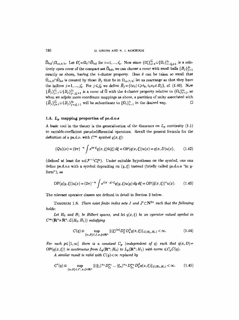
1.3. Lp m a p p i n g p r o p e r t i e s o f ps .d ,o . s
A basic tool in the theory is the generalization of the theorems on Lp continuity (1.1)
to variable-coefficient pseudodifferential operators. Recall the general formula for the
definition of a ps.d.o, with C ~ symbol q(x, ~):
( Qu)(x) = (2~r) ~ / eiX'~q(x, ~)~(~) d~ = OP(q(x, ~) )u(x) = q(x, D)u(x), (1.42)
(defined at least for uC~Y-IC~). Under suitable hypotheses on the symbol, one can
define ps.d.o.s with a symbol depending on (y, ~) instead (briefly called ps.d.o.s "in y- form ), as
(21r)-~ / ei(X-u)'~q(y, f)u(y) dy d( = OP(q(x, ~))*u(x). (1.43) OP(q(y,
The relevant operator classes are defined in detail in Section 2 below�9
THEOREM 1.6. There exist finite index sets J and J ' c N 2~ such that the following holds:
Let Ho and H1 be Hilbert spaces, and let q(x, ~) be an operator valued symbol in C~r Rn; ~(H0,//1)) satisfying
C(q) - sup II(~)I~fD~D~q(x,~)IIL(Ho,H1) < oo. (1.44)
For each pE]l , ov[ there is a constant Cp (independent of q) such that q(x,D)= OP(q(x,~)) is continuous from Lp(Rn;Ho) to Lp(Rn;H1) with norm <~ CpC(q).
A similar result is valid with C(q)<oc replaced by
C ' (q) - sup 11(51)~1D~ ~n a , D e (1.45) ... (~,~) D ~ xq(x,5)tl~(Ho,H,) <oo. ( a ,~}EJ ' , x , ~ R . ~

A GLOBAL CALCULUS 181
The results hold also for operators given in y-form OP(q(y, ~)), when q(y, ~) satisfies (1.44) resp. (1.45) with x replaced by y.
Indications of proof. (1.44) and (1.45) are generalizations of, respectively, Mihlin's
and Lizorkin's criteria (!.1). For (1.44), the proof of Hbrmander [HI, Theorem 3.5], although formulated for the L2 case, applies to the abovementioned Lp case by use of Mihlin's theorem in a Hilbert space valued variant (cf. [B-L, Theorem 6.1.6], IT1, 2.2.4]);
this shows that one can take J={{a,/3}cN~'~l [ a l , [~ l~n+l }. Statements requiring fewer values of ~ (and of a, when p~ 2) can be found e,g. in Nagase [Na], With J replaced
by N 2~, the Lp continuity of polyhomogeneous ps.d.o.s is shown in Seeley [Se2], and Beals [B] includes the S~ case. - - For (1,45), let us first observe that Lizorkin's constant coefficient result generalizes to Hilbert space valued operators e.g. by the argument given in Shamir [Sh] for reducing Lizorkin's result to a version of Mihlin's result. The present
authors have worked out a generalization of the proof of [HI, Theorem 3.5], that shows that one can take J'={{a,~}eN2nlai<2 for j = l .... ,n, I~l~<n+2} in (1.45) (for lack of space, we shall not include the details here). Yamazaki [Y] shows that one can take
J' ={ {a,/~}eN2~]a={~jaj}i=l,..,,n with aj<n+ l, for j=l , ...,n, ]/~1<1},
Finally, when an operator is given in y-form OP(q(y,~)), we simply use that its adjoint satisfies OP(q(y,~))'=OP(~(x,~)) (cf. (1.43)), where q(x,~) has the required
estimates (1.44) resp, (1.45) as an operator from/-/1 to H0 for each (x, ~). Then, by the preceding results, OP(q(x, ~)) is continuous from Lp(R~; H1) to Lp(l:tn; H0) for all
pE ]1, c~[ with a bound CpC(q) resp. CpC'(q), so it follows by duality that OP(q(y, ~)) has the asserted continuity properties. []
Remark 1.7. The theorem does not extend to the general case where H0 and/ /1 are replaced by Banach spaces. As a simple illustration, we mention the fact that the Poisson operator K with symbol (~'):/P((~')+i~) ~1 (and symbol-kernel (~')l/PH(xn)e-(~')z", H(xn)=I{~>o}) is not continuous from Lp(R n- l ) to Lp(R~_) when p<2 and n > l , just continuous from the strict subspace B~ n- l ) to Lp(R~), cf. [G3, Remark 3.3]. For
n=l, K is continuous from C to Lp(R+), and if Theorem 1.6 (in dimension n - 1 ) could be used for the mapping q(x',~'):v~(~')l/Pe-(r with Ho=C, HI=Lp(R+), the
Lp-continuity of K for n > 1 would follow.
In our approach to L v estimates for the boundary operators in the parameter- dependent calculus, we apply the above theorem to symbols depending on the tangential
variables, valued in spaces of functions (or distributions) in the normal variable. A fun- damental idea is to choose these spaces, that must be Hilbert spaces, in such a way that they give spaces contained in Lp by interpolation. Here we use the L2 Sobolev spaces

182 G. GRUBB AND N. J. KOKHOLM
over R+ , and the weighted L2 spaces:
L2(R+,x~)={veD'(R+)tx~v(xn)eL2(R+)}, 5 e R . (1.46)
Note that the dual space of L2(R+,x~) (in relation to the sesquilinear duality
fR+ u(xn)O(xn) dx,,) is
L2(R+, x~)* = L2(R+, x;~). (1.47)
More precisely, we shall use:
T H E O R E M 1 .8 . (1) / ] 1 <p<~2 andS' < ~ 1 - 1 < 6 , thenwith 0 = ( ~ - - ~ - - 5 1 1 ' ) / ( 6 - - 6 ! ) ,
5 t (L2(R+, x,~ ), L2 (R+, x~))O,p C Lp(R+),
(1.48) (H~; o (R+), H~;~(R+))o,p D Lp(R+).
(2) / ] 2 ~ p < c ~ andS'<�89 -1~<5, then with O=( �89 -5')/(5-5'),
(Hi' (~t+ ), H~(~t+ ))o,v C Lv(R+), (1.49)
(L2 (R+, x~'), L2(R+, x~))e,v D Lp(R+).
(The inclusions are identities when p=2.)
Proof. The identities are classical for p=2; it is the case p r that demands a special
argumentation.
The first line in (1) follows for general 6' from Gilbert [Gi]. By HSlder's inequality,
p -- IIflIL,(~+) -- k-,<=~'-~<~k xnpe' Jx~ f(xn)l p dxn
, "[p/2
The last expression gives by [Gi, Theorem (3.7)0)] a norm on the interpolation space on
the left hand side of the first line in (1.48), and hence this inclusion follows. (We observe
that in the result of Gilbert, 2 k-1 <w(x) ~< 2 k should have been written 2 k-1 <w(x) -1 < 2 k,
cf. [Gi, Theorem (3.3)].) The second line in (1.49) follows by duality. When 5'=0, a simpler argument suffices, where R + is just divided into ]0, a[ and [a, oo[, HSlder's
inequality is applied, and a is chosen so that the two terms balance.
To show the first line in (1.49), we use that
51 - - (H~ (R+), H~(~+))0,v = B~/~-~/P(~t+ ) c H~ ) = Lv(R+),

A G L O B A L C A L C U L U S 183
where the first identity is accounted for in IT1, 2.10.1], and the inclusion (which is an
identity for p--2) follows for p>2 from [T1, 2.8.1 (18)], cf. also [T1, 4.6.1]. The second
line in (1.48) follows by duality. []
As an immediate consequence we get (using e.g. [B-L, 5.8.6]):
COROLLARY 1.9. (1) I l l<p<.2 and ~,<~1�89 then with 8 = ( ~ - � 8 9
(4(R~-1; L2(R+, z~ )), Lp(R~-~; L2(R+, x~)))e,p c 4(R~), (1.50)
(Lp(R~-~; H~.o~'(K+)), Lp(R~-~; H~;6o(~t+)))o,~ �9 L~(R~). 1 1 1 1 ~ / (2) / f 2~p<c~ and ~ ' < ~ - ~ < ~ , then with O = ( ~ - ~ - ~ f ) / (~ -~ ),
(L~(R~-~; H~ (R+)), 4(R~-1; H~(R+)))~,~ c 4(R~), (1.51)
(Lp(Rn-i;'L~(R+, Xn~')) , /v(Rn-1; 52(R+, x~)))e,p �9 Lv(R~). (The inclusions are identities when p=2.)
2. Uniformly estimated symbols
2.1. Symbol spaces
We shall now supplement the symbol spaces introduced in [G2] with spaces of symbols
satisfying estimates that are uniform in x resp. x', following the pattern set up for ps.d.o.s
in HSrmander [H3, Chapter 18]. Besides that this leads to operators with convenient
continuity properties in global Sobolev spaces relative to R~_, this has the advantage that
the rules of calculus can be stated in a more exact form than for the symbols satisfying
local estimates: To take an adjoint or to compose two operators leads to an operator with
a precisely defined symbol in the appropriate space, not just defined modulo so-called
negligible operators. (Recall from [G2] that there are many different kinds of negligible
operators involved in the local parameter-dependent calculus: one for each regularity
number and for each operator type, and some additional ones.)
The symbols will depend on a space variable generally called X E R nl and later
specialized to be x E R ~, x' E R ~-1, (x, y) E R 2n or (x', y ' )ER 2n-2, etc.
To avoid lengthy repetitions, we simply use the notation from [G2] and refer the
reader to the details there, recalling only a few conventions, such as
Dxj = -iO~j ; Dx~ = +iO~ ;
(~-f)(~) -- d d (2.1)
a• =max{+a,0}; (~, g) = (1~12+g2+1) '/2, ~,(~,~)=(~)/(~,~), dg,~)=(g)/(g,~), ~<(g,~)=(g,~).

184 G, GRUBB AND N. J. KOKHOLM
Occasionally, it can be useful to redefine (~, #) as
(~, ~) ~-- (i~I2d-l-#2d-{- 1)1/2d (2.2)
or
u) = (l U+u2d) TM for u)i 1 (2.3)
(extended to be smooth positive), where d is a fixed positive integer; these are useful for holomorphic extensions in/~ and homogeneous symbols, e.g. in connection with resolvent studies ([G2, 5]). Observe also:
(()v(~'#)d-u+(~'#)d=(g(~'#)V+l)(~'#)d~-- { (~)~ (~, #)d-v (~, #)d whenWhen u~0,u~>0' (2,4)
We shall use the conventions: ~ (resp, >/) means "4 (resp,/>) a constant (indepen- dent of the space variable) times", Moreover, -" means that both ~ and ) hold, The constants vary from case to case.
Recall (e.g. from [G2, 2.2]) that for rEZ, 7~-1 is the space of functions f(~n)E C~162 that have an asymptotic expansion ~ _ ~ < j ~ _ ~ s j ~ for I(~l-ooo; and 7~= ~J~ez 7/~-1. Moreover, 7i + is the subspace of H-1 consisting of functions extending holomorphically into C_ ={~n E C Jim ~n <0} with the same asymptotics there, and 7/- is the direct sum of the space of complex conjugates of 7/+ and the space C[~.] of polyno- mials. For a simple formulation of symbols of negative class it is conwenient to introduce the notation
We recall that 7-/=7"/_1A-C[~], 7-/=~/+47~- (direct sums) and 7/_1=7/+ @7/=1 (ortho- gonal direct sum in L2(R)); the projections onto ~/-1, 7/+, 7/- and 7/- 1 being denoted
h- l , h +, h- resp. h-- 1. We denote by S~o(Rn• n) the space called S d or Sd(RnxR n) in [H3, Chapter 18]~
consisting of symbols p(x, ()EC~(R~x R n) satisfying the estimates (on Rn• Rn):
for all
The subspace of polyhomogeneous symbols (called 8vdhg(R"xRn ) in [H3, Chapter 18]) will here be denoted Sd(RnxR"). The definitions generalize immediately to the case where xER n is replaced by by X ER m . Now let us define parameter-dependent symbols:
DEFINITION 2.1. Let d and uER,

A GLOBAL CALCULUS 185
r t~,~l .. ~n+ ~ ~ of X-uni formly estimated (or just: uniformly esti- (1) The space ~,1,0,.~ ^ ~ + )
mated) pseudodifferential symbols of order d and regularity u consists of the C ~ functions
~n~+n+ l satisfying the estimates p ( x , ~ , i t ) on +
tD~ O? D~p(X, ~, U)t ~- ( (~V -I~ (~, U) d-~-~ + <~, ~>d- t~l-J) (2.7)
= (0(~, It)~-lal + 1)(~, p)d-lal-#,
for all indices a E N n, 13EN n~, j E N .
(2) The space Sd,~ tR '~x l~ +~'~ + j of uniformly estimated polyhomogeneous ps.d.o. d,v n1 - - n + l symbols of order d and regularity ~ consists of the symbols pESx,0(R • ) that
moreover have asymptotic expansions P ' ~ I ~ N Pd-l, in the sense that P - - ~ t < N Pd-l be-
lo~g~ to ~ ~,~- ~ (it"~ • ~t~ + ~ ) for an N e N , and Pd-~( i , ~, It) ~ homogeneous of d ~ e e
d - l in (~, It) for [~t >11.
(3) A symbol p(x, y, ~, it) E sd~ (R2nx ~.~_+1) is said to satisfy the uniform two-sided
transmission condition at xn=yn=O, when p and its derivatives at xn=Yn=O are in
TI as functions of ~n, m such a way that the estimates required in connection with the
asymptotic expansions in ~n (el. [G2, Definition 2.2.7]) hold with constants independent
of (xr,~r). This can also be expressed as the property that for all indices j, N, NV E N and
a,13, "yEN '~, the restrictions to zn E P ~ of the inverse Fourier transforms,
4- N N ' --1 ~ 7 a " t t ri z , D~. ~ _.r D ~ D u D r 1T~p(x , O, y , O, ~',~,~, It), (2.8)
are bounded functions of ( x~, y~, z , ) E R n - I • R n - l x R • (hence extend to C ~ functions
of (x',o~ z ~eR~, " - ~ . , . , • ,. The space of such symbols is denoted S~:~,utt,(R2'~• and d ,u 2n - - n + l the subspace o] symbols that moreover are polyhomogeneous is denoted Suttr(R xl~+ ).
Similar definitions are made when p is independent of y or x (then R ~n is replaced by
It").
The definitions (I) and (2) are straightforward generalizations of the definitions in
[G2, Sections 2.1 and 2.21. As for the transmission condition, a further analysis is given
in Grubb and HSrmander [G-H] and [G4, 1.3]. In order for a ps.d.o. P=OP(p(x,~))
to have what was originally called the transmi~ion property (on R~_), namely that
P ~ preserves the property of being C ~ on ITS_, it is necessary and sufficient that r + ~ N T - - 1 D ~ D a ~ ' J q d C o o z,'.n - r ~ ,0,~) is for (x~ ,zn)ERn- lx f f {+, for all indices (no require-
meat is needed for zn <0). However, the full IXseudodifferential boundary operator cal-
culus needs the preservation of C ~ property for both P and its adjoint, or equivalently,
the preservation of C ~ property for P on both R_'~ and R~_. But here, when d is integer
and P is polyhomogeneous (the case mainly considered in [G21), one can show that the
two-sided preservation of Coo property (on R~_ and It,,_) is equivalent with the one-sided

186 G. GRUBB AND N. J. KOKHOLM
preservation of C ~ property ion R~). The transmission condition used in [G2] was
indicated there by a subscript 'tr'. In [G-HI, spaces of symbols with the one-sided (resp.
one-sided uniform) transmission property were indicated by a subscript 'tr' (resp. 'utr').
In the present work, we allow noninteger d in the study of mapping properties, and we
indicate the spaces of symbols satisfying the uniform two-sided transmission condition by
the subscript 'uttr', to avoid conflict with earlier conventions. Since this is the condition
used from now on, we often just say that such symbols satisfy "the uniform transmission
condition".
For fixed #, Definition 2.1 (3) gives the space d 2,~ ,~ S1,0,uttr(R x t t ) of parameter-inde- pendent ps.d.o, symbols of order d satisfying the uniform two-sided transmission condi-
tion.
Now let us define the uniform versions of the boundary operator symbol spaces.
DEFINITION 2.2. Let d, v e R and f e Z . The spaces S~:~(itn~xR~_,K:) (]C=7-/+,
~ - 1 resp. 7-l+@7-lr_1) of X-uniformly estimated Poisson, trace resp. singular Green symbols of degree d, class r and regularity v consist of the symbols in qd,~(~n~ ~n K.) ~ i , 0 k ~ " , " '~+,
(cf. [G2, Section 2.3]) satisfying the estimates listed there with constants independent of X E R TM .
Expressed in detail, with 0=0(~',~), '~=(~',~) (4. (2.1)):
(1) The space Sf:~ (R n' x R.~_, 7-i +) of uniformly estimated Poisson symbols of order d + l (degree d) and regularity v consists of the functions k (X , ( ,# ) lying in 7-I + with
respect to (n and satisfying estimates
+ r ~ "~ "~' J ( 0 ~ - I ~ I - [ ' ~ - m ' ] + + l ) x a + l / 2 - 1 ~ l - ' ~ + m ' - j , (2 .9)
for all indices.
(2) The space Sld:~'(R'UxR._~,7-/~-_x) of uniformly estimated trace symbols of order and degree d, regularity v and class r consists of the functions t(X, ~, #) of the form
t(x,r (2.10) 0<~j<r+
where sj(X,~',#)Esd~J'~(R'UxR~_) and t ' (X , ( ,#) is in 7-/~i~{_i,~_I} as a function of
~n, with estimates
{]h-I D~x D~,D~ ~ ' D ~ t' ( X, ~, ~)IIL2.,. ~- (0 ~-I~t-[m-~']+ +1) xd+ l/2-1~l-m+m'-~, (2.11)
for all indices. (The space Sla:~(it'UxR~, 7-/+_1) is defined similarly.) (3) The space Sd:~'(R'UxR~_,7-/+@?-/~-_l) of uniformly estimated singular Green
symbols of order d + l (degree d), regularity v and class r consists of the functions

A G L O B A L C A L C U L U S 187
g(X, (, ~. , It) of the form
g(X,r it)= E kj(X'r +g'(X'~'r]"'it)' (2.12) 0<~/<r+
s d - J , v r R n l x ~ l y 7-~+~ wherekj(X,{, i t )e 1.o ~ +, j andg'(X,~,7?n,it) isinT-t+@n2~in{_l,r_l} asa function of (~n, ~?n), with estimates
+ - r a k k' m m' j , [lh~. h_l,~. Dx D~, D~. ~n Do. ~n D,g i X, ~, ~ , It)I[ L2.,..,. (R~) (2.13)
(ev-Ial-[k-k'l+-[rn-m']+ + 1)xd+l/2-la[ -k+k'-m+m'-j,
for all indices. (4) The spaces Sd'V(R"lx fitS_, E) of uniformly estimated polyhomogeneous ps.d.o.
symbols of degree d and regularity v consist of the symbols feS~(R'~• that moreover have asymptotic expansions f " ~ t e N fd-t, in the sense that f - -~ t<N fd-t E S d ~ o N ' V - N ( I : I , n l • for all NEN, and f d - l ( X , ~ , i t ) resp . f d _ l ( X , ~ , ? T n , i t ) i s homo- geneous of degree d - l in (~,it) resp. (~ ,~ ,#) for I~'1>~1.
(5) There is a similar convention for the associated spaces of symbol-kernels k= J:~kz k, { = ~ k z t and ~=f fr ( lx ~';l__,u,g (cf. (2.1)) when r~<0; here/C=7"/+, 7"~: 1
resp. 7-t+@7-t-~ is replaced by S(~t+), S(~t+) resp. S(fft2++) (with R~_+=m• and
the estimates are replaced by the following, where f =[~ or t~,
j3 m m' a j~ ! llDxxn 9=. DuD.f(X , xn, ~ , It)llL~,~. (rt+) ~ (e ~-t~-m'l+-l~1 +I) M+~n-'~+m'-l~l-j, I l " ~ I IID~xxkOk y~D~ D~,D~g (X,x,,y,~, ' . . 2 ~, It)l L2 . . u.(R++) (2.14)
(t)v- [k- k'l+ -fro-re'f+-[al +l)~d+l--k+k'--m+m'-[aI-j.
The parameter-independent boundary symbol spaces (generalizing [BM2]) have a
simpler definition, without the powers of ~ and without reference to a v. To save space
we just write:
DEFINITION 2.3. The spaces of uniformly X-estimated boundary symbols of degree d and class r are defined as in Definition 2.2, considered for a fixed It.
For the uniformly estimated symbols there axe the same inclusions of the parameter-
independent spaces in the parameter-dependent spaces as described in [G2, Proposition
2.3.14]. The definition of symbols of negative class is consistent with that of [G3, 4].
We now have to show that the calculus for operators defined from these symbols
works in a precise way, as indicated in the introduction. In principle, this requires going
through the whole development of [G2, Chapter 2] for the new symbol classes; however,
much of what has to be done is so close to the development there that it suffices to give
some indications, drawing also on the presentation in [H3].
13 - 935204 Acta Mathematica 171. lmprim6 le 2 f~vrier 1994

188 G. GRUBB AND N. J. KOKHOLM
2.2. Composition rules for ps.d.o.s
Let p(x,~,#)Esd~(Rn• n+l~+ /. For each #El=t+ it follows from [H3, 18.1] that P~=
OP(p(x, ~, #))=p(x, D, #), defined by
~, #))u(x) = (2r) -'~ f eiX'r ~, #)fi(~) d~, (2.15) P,u(x) OP(p(x,
maps S (R ~) into itself, extending to a continuous mapping of S ' (R n) into itself, with Schwartz kernel tgp(x, y, #) related to p(x, ~, #) by
)~p(x, y, #) = (2~) -~ ./e~(~-Y)'~p(x, ~, it) d~ (2.16)
(identifiable with Jr~zp(x, ~, it)tz=~-~);
The integral in (2.16) is an oscillatory integral, cf. [H3, 7.8], it is the limit for e--*0 of the expressions obtained by multiplying the integrand by a function X(e~), x E C ~ ( R n ) with
X=I on a neighborhood of 0 (cf. also (2.22) below). Operators and symbols of order -00 will be called negligible.
Recall from [G2] the simple inequalities:
(~)~(~,#)-~'~. (~)~+l~'l(it)-v'; (~),,{it}-u'~ (~)~+lv'l(~,it)-v'; (2.18)
showing how a decrease for litl--*~ carries over to a decrease for I((, it)l --*~ and vice versa (with a certain loss of precision in the ~-variable). They can be used, together with
elementary properties of the Fourier transform, to show the following characterization of the present negligible symbols of regularity v ~ in terms of kernel properties:
--~o,~/--oe n - - n + l __ - - N , v ~ - N n LEMMA 2.4. I fp(x ,~,u)ES (R x R + ) - - O N S l , 0 (R xR~_+I), i.e.,
}D~D~DJp(x,~,it)l ~ (~)--N(#)--u'--j for all (~,~eN '~, j, N E N , (2.19)
then
"~ J X ' ' " ]D~D~Dut:p(x, - z , it)i~(z) - y (it)-~-~ f o r a l l % B e N ~, j , N ' E N . (2.20)
Conversely, if ]Cp(x, y, it) is a function satisfying (2.20), then the function p derived from it by (2.17) satisfies (2.19), hence is a symbol in S-~ ' " ' -~ (R~• +1) defining the operator with kernel ]Cp. (For fixed it, this characterizes the negligible ps.d.o.s in the standard uniform calculus.)
The proof is straightforward and consists of showing that each estimate in (2.20) follows from a certain finite set of estimates (2.19) and vice versa, where the number of

A G L O B A L C A L C U L U S 189
estimates grows with the size of the indices. Note the advantage of the present calculus:
The operators with C ~ kernels (satisfying suitable estimates in x, y and #) belong to
the calculus, and do not have to be treated as residual classes as in [G2].
Proposition 18.1.3 in [H3] extends readily to the parameter-dependent situation,
showing that for any sequence of symbols Pd-I E S~o l'~'-l(R '~1 x ~_+1) (i �9 N) there exists a symbol pE S~l~(anix R.~ +1) such that P--~I<M ~d-Z- ~c"d-M'~'-MIRn'XI{.n+l~ol,O ~ + j for any
MEN. We then say that p N ~ l e N Pd-*~ Now it is also of interest to consider ps.d.o.s represented by formulas (as in [H2])
(27r) - '~//ei(~-~t)'~p(x, y, ~, #)u(y) dy d~ = OP(p(z, y, ~, #) )u(x),
uE$(Rn), where p(x, y, ~, #)�9 ~_+1). When p is not integrabte in ~, this is
interpreted, via oscillatory integrals (cf. [H3, 7.8])) by a weak definition as follows: For u, vES(R n) we set
( P~,u, v) = ~(2~r ) - n / / f ei(~-v)'~p(x, y, ~, #)u(y)~(x)x(v~) dx dy d~ (2.22)
= lim(P,,,u, v), P,,~ ~ OP(p(x, y, ~, #)X(e~)); e~--.0
this defines P~ as an operator from S(R") to S'(Rn), The formulas imply
Pv,, = OP(q,(x, ~, #)), where qe(x, ~, , ) -- e 'Du'~ (p(x, y, ~, ~u)X(*~))I~=,,
as defined in [H3] before Theorem 18.1.7; and the results on convergence of symbols
there ([H3, Theorem 18.1.7 and Remark]) show that q~(x,~,p) converges weakly in
Sld, o (RnxR a) for each ~ to
q(x,~,t~)=e~D~.Dcp(x,y,~,p)]~= x,., ~ 1 ~,~DC,~r ~eN" (2,23)
with OP(p(x, y, ~,/~)) = OP(q(x, ~,/~)).
That q,(x, ~) ---*0 weakly in Sl~,o(Rnx R n) for ,--*0, ~E ]0, 1], means that the set {q,},e ]0,1]
is bounded in S~,0(Rnx R '~) and q,---,0 in D~(R2n); the latter convergence can be sharp-
ened to uniform convergence of D~D'~q~(x, ~) for all a, B~N" on the compact subsets of R 2~.
To avoid repetitions, we have a ]~ in the notation here, but up until Theorem 2.7, it
should be considered as a fixed number.
For the special case of (2.21) where p is independent of x, (2.23) implies
OP(p(y,~,p))=OP(ql(x,~,l~)), with
ql(x,~,l.~)=eiD~'D'p(y,~,l~)]~=~,'.~ ~ ~0~1 ,XD,~p(y,~,#) ~=~" (2.24) h E N "

190 G. G R U B B AND N. J. K O K H O L M
We observe furthermore that , by (2.22), the adjoint of Pg=OP(p(x , ( ,#) ) is P ~ =
OP(p(y, (, It)), which may be reduced by (2.24), so that we get:
OP(p(x, ~, It))* = OP(/~(y, ~, It)) = OP(q(x, ~, It)), with
q(x,~, It) = e 't)~'DCp(x, ~, It) ,.~ E ~O~D~p(x,~,it),l a •- . (2.25) ~ c N n
cf. also [H3, (18.1.9)]. Note that then P~=OP(q(x,~,it))*=OP(~-l(y,~,it)), so that we also find (by conjugation of the formula for q, cf. (2.1) for D~):
OP(p(x, ~, It)) = OP(q2(y, ~, It)), with
q2(Y'~'it)=e-iD~'Dcp(x'~'it)[z=u'" E ~O;D~p(z,~, i t)]x:y. (2.26) h E N '~
This prepares for the formula for the composition of two operators, cf. [H3, Theorem 18.1.8]:
OP(p~ (x, r It)) OP(p2 (x, r It)) = OP(q(x, r It)), with
q(x, ~, It) = e iD~''o" (Pl (x, ~1, It)P2 (Y, ~, It))]u=:~,,/=~
'~ E l~aDa" (2.27) h-?.,% n kPl (x, ~?, It)P2(Y, ~, It))ly=z,n=~, a E N n
denoted q(x, ,~, It) ---pl(x, ~, It)op2 (x, ~, It).
The formula can (as in [H2] and [G2]) be derived from the preceding rules, by first using
(2.26) to construct q2(Y, ~, It) such that OP(p2(x, ~, It))--OP(q2(y, ~, It)), next observing that one has the simple product formula
OP(pl (x, ~, #)) OP(q2 (y, ~, #)) = OP(pl (x, (, #)q2 (Y, ~, #)),
and finally reducing Pl (x, ~, It)q2 (y, ~, It) to q(x, ~, #) by use of (2.23) and a certain formula for simplification of binomial expressions.
Finally, we have to discuss coordinate changes. Here [H3, Theorem 18.1.17] is only formulated for symbols with compactly supported kernels, but the hypothesis of com-
pactness can be removed when admissible diffeomorphisms are considered, cf. Section 1.2, as follows: Let U and U~, be open sets in R n, and let x: U---*U~ be an admissible
diffeomorphism. Let Pu=OP(p(x, ~, #)) be a ps.d.o, with distribution kernel supported in a subset of U • U with positive distance from O(U x U). Then it induces a ps.d.o, on
V by (Pu,~,u)ox=Pu(uox) for ueC~(U,~) , with
p,~(x(x), 7, #) = e-i~'(~)'n Pt,( ei~'(x)'n) (2.28)
,x~ E 1 D,~ "x t , ~, iox(y).,1 , , p t , I t ) o ; e a E N n

A GLOBAL CALCULUS 191
where Qx(y )=g(y ) -g (x ) -~ (x ) (y -x ) . This is seen by a generalization of the proof of
[H3, Theorem 18.1.17]: Let X(x)EC~(R n) with x = l near 0, and write the distribution
kernel ]Cp(x, y, #) of P~ as a sum of two terms/C 1 =(1 -X(x-y))lCp and ~2 =X(x-y)ICp. Here/~1 is the kernel of an operator of order -oc , and the estimates assuring this ((2.20)
with fixed #) carry over to the corresponding kernel ~ in view of (1.39). Concerning
]C 2, we note that the estimates in [H3, Theorem 18.1.17] are valid, uniformly in a E R n,
when ]C 2 is replaced by ~o(x+a)r 2 with ~o and CEC~. Taking ~o and r equal to 1
on a sufficiently large neighborhood of 0, we can obtain that for any (x, y) Esupp X(x-y) there is an a so that ~o(x+a)r there, so the desired estimates hold for ]C 2.
(These arguments were kindly supplied by L. HSrmander in a personal communication.)
We say as in [G2], with a somewhat loose terminology, that Pu is in x-form, (x, y)-
form, resp. y-form, when it is defined as in (2.15), (2.21), resp. (2.21) with p(x, y, ~, ~) replaced by p(y, ~, #). We shall also sometimes need a mixture of these concepts; e.g.
an operator defined by (2.21) with p(x, y, ~, #) replaced by p(x', yn, ~, #) is said to be in
(x', y,~)-form. One changes an x-form to an (x r, yn)-form by a variant of (2.26), namely
OP(p(x, ~, #)) = OP(q(x', y~, ~, #)), with
q(x',y~,~,]z) =e-iDv~De~p(x,~,#),.~ ~ 70~D~,p(1 " - j x, ~, #)]~=y~. (2.29)
jEN
The above considerations describe the basic rules of calculus for ps.d.o.s when # is
fixed. For the parameter-dependent calculus, we moreover have to justify the asymptotic
cd,~/~n~ ~+~). This will expansions (2.23) etc. with respect to the symbol spaces ~1,0 ~-~
be based on the following general rule inferred from [H3, Theorem 18.1.7 ft., Theorem
18.4.11]:
LEMMA 2.5. Let B be a Banach space, and let S~,0(RnxRn)| be the space of C ~ functions a(x,~) from a n x R n to B satisfying [[D~D~a(x,~)[[s~(~) d-I"], for all a , ~ E N n. Then a(x,~)~-~eiD,'Dea(x,~) extends from a mapping in S(RnxR'~) | to a weakly continuous mapping from Sd,o(Rn• R n) | to sd,0(Rnx R n) | B; and for each kEN, the mapping Rk defined by
Rk: a(x, ~) H eiD~'Dea(x, ~)-- ~ ~O~D~a(x, ~) I~l<k
is weakly continuous from Sax,o (R'~x R") | to sd~k(R"x R '~) |
Remark 2.6. For AES(Rnx Rn) | the Fourier transform A=~'(~,r is de-
fined by the usual formula and . 4ES(RnxRn) | by the standard proof. This allows
us to define e~D"DcA(x,~)ES(R~xRn)| in the usual way, cf. [H3, Volume I, p. 207].

!92 G. G R U B B A N D N. .t. K O K H O L M
- - As in [H3, Definition 18.4.9], we say that a mapping from sd~,o| to sd:,o| is
weakly continuous when it is continuous in the ordinary sense (with respect to the Fr6zhet
topologies) and, in addition, the restriction to a bounded subset is continuous in the C ~
topology.
Proof of Lemma 2.5. For AES(R'~xRn) | b*EB*, one has that (b*,A)ES and
(b~, e iD~'D' A(x, r l = eiD~'D' (b*, A(x, ~) ). (2.30)
Define the seminorms on Sd, o@B, IAik,s=supt~l+l~l<k sup~,r I](r162 (This can also be reformulated in the notation of [H3, 18.4].) The proof of [H3, (18.4.17)]
gives for aE Sld,0 (with the special partition of unity ~v E C ~ used there): For any N there
is an M and a C (depending only on the dimension and the choice of metric and partition
of unity) such that
<
~ 0 m this we get by use of (2.30) for AESd, o| with the same constants:
II eio~'Dr ( w A )(x, 5) I[- ~< C( l + d~(x, 5) )-N (5)dlAIM, B.
Hence we have for AESdl,o|
II er162 (v~A )(x, ~)[l" ~< C ' (5)dIAIM,B �9 V
We can therefore define (eiD~'DcA)(x, ~ ) = ~ v eiD~'Dr (~pvA)(x, ~) as a weakly continuous
mapping from Sal,o| to B (cf. [Ha, Theorem 18.4.10]). Estimates of derivatives and
remainders follow easily, and give [H3, Theorem 18.4.11] for Sdl,o| []
The lemma will be used with B=f~(H1,H2) for Hilbert spaces /-/.1 and/-/2 in the
study of ps.d. boundary operators. For the ps.d.o.s we use it with B = C to obtain:
d,v 2 n THEOREM 2.7. For p(x, y, ~, #) E $1, o (It x ~ + 1 ) , the asymptotic expansion (2.23)
holds in ~'l,0r . . . . + j. Moreover, when p(x,~,~)ESdl[o(l:tn• the asymptotic expansions (2.24), (2.25) and (2.26) hold in 8!, o (It x
When It xR , ( ;~ .+ ) ]or i=1 ,2 , the asymptotic expansion (2.27) ~dl+d2,m(Vl,V2),'~n ~ . n + l - holds: in i,o (I t • ), where
m(,1, v2) = rain{v1, v2, v, +"2}- (2,.31)
Hence when Pi,, (i = !, 2) are parameter-dependent ps, d. o.s of order di and regularity ~i, with uniformly estimated symbols, then the adjoint P{,, and the composition Q~=

A G L O B A L CALCULUS 193
Pl,uP2,u are parameter-dependent ps.d.o.s with uniformly estimated symbols, of order dx resp. dl+d2 and regularity ul resp. rn(ul, u2). Here Qu satisfies the uniform transmission condition when Pl,u and P2,u do so.
The operator classes are invariant under admissible coordinate changes, satisfying rules as in (2.28).
Proof. We first treat (2.23), from which the statements on (2.24), (2.25) and (2.26)
follow. Let q'(x, y, ~, ~)----eiDuDcp(x, y, ~, #), then q(x, ~, ~)=q'(x, x, ~, #). Since (x, #)~--~
p(x, . , . ,#) is C r162 with values in Sd, o(RnxRn), the same is true for (z,#)~-*q'(x, .,. ,#). In particular, q' and q are C ~ .
Now we shall show that q satisfies the first seminorm estimate for the space s d , v (l:~ 2 n v ~ n + 1 "~.
1,0 k ~ ' ' ~" "~ - I - ] "
Iq(x,C ~)1 ~ (~, ~)d+(~, p)d-~(~)~. (2.32)
Note that for large 7 (]71> ~) and general c~,fl one has that
cf. (2.18). It follows that (y, ~)~-}D'~p(x, y, ~, #) belongs to S~+la-'l-I~ll,0 ~(Rnx R '~) with
seminorms that are O((#) d-~) uniformly in x. According to Lemma 2.5, we have for
kCN if I~/l>v,
but also for general f~ if k>d,
1 a D O x
- , 0 a s
Choosing k>21dI-t-21ul+l, we get by h'l integrations of the radial derivatives of q' along
rays from 0% using (2.33) and (2.34), that
I~l<k
which implies (2.32).

194 G. G R U B B AND N. J. K O K H O L M
Since Dx,~,~,~ commutes with e iD~'Dr and b~D~, all other estimates of q in
sd~(R~• ~_+1) follow immediately, and the expansion in the full asymptotic series (2.23)
follows by taking k even larger in (2.33). This implies the first part of the theorem.
For the second part we proceed as indicated after (2.27) above. The rule for (2.26)
proved above implies that the expansion of q2(Y,~, #) holds in sd2'~2twn• +1) Now 1,0 k~*" ~, d l+d" ,m(~ ' l , v " ) / ' ~2nvDn+l~ [G2, Proposition 2.1.5] shows that pl(x, ~, ~)q2(y, ~, e06S1,0 ~ . . . . . + ~ with
m(~'l, u2) defined by (2.31). Then by the rule for (2.23), the expansion of q(x, ~, #) holds in s d l Td2,m(Ul,U2) []:~n v ]~ n + l ~
1,0 \ . . . . ~+ ,'"
The third statement is an immediate consequence, and the rules for coordinate
changes follow by an extension of the proof described after (2.28) including the #-
dependence. []
2.3. B o u n d a r y opera to rs
Recall from [G2] the defining formulas for a Poisson operator Kg, a trace operator T~
of class 0 and a singular Green operator G~, of class 0, in terms of symbol-kernels (cf.
Definition 2.2 (5)):
K~v(x) = OPK ( k(x', ~, # ) )v(x) = OPK (/r ~', #) )v(x)
= (27r) 1-n . / , ,_ , e ix''r fc(x', xn, {', #) 0({') d{',
T~u(x') = OPT (t'(x', ~, #))u(x') = OPT ({'(x, ~', #))u(x') (2.35)
= (21r) 1-'~ e i#'r t'(x',xn,~',#)d(~',xn)dxnd~', n - 1
G~u(x) = OPG(g'(x', ~, y~, #))u(x) = OPG(~'(x, Yn, ~', #))u(x)
= (2~) 1-n J ~ ' ~'(x', ~n, y.~, ~ ' , . ) aft ' , ~ ) dy~ d~'; n - I
here ~(()=7~_~u(x), ~((')=~'~,_~,v(x'), and a(~',x,~)=~'~,__.~,~(x',x,~). (See e.g. [G2, 2.4] for the definitions in terms of symbols.) When the class r is />0, the trace
and singular Green symbols are of the form
t(~',~,.)= ~_. ~Ax',r o~<j~<~-I (2.36)
g(~',~,~,~)= ~ kAx',~,~)~+g'(x',~,~n,~), o<<.j<<.~-I
cf. (2.10), (2.12).
by T.=
Then we define T~=OPT(t(x', ~, #)) resp. G~ =OPG(g(x', ~, ~n, #)),
E Sj,,Tj+T~, resp. G,= E KJ,,~/J+G~ , (2.37) 0 ~ j ~ r - - 1 O~j~r--1

A GLOBAL CALCULUS 195
where Suj =OP'(s j (x ' , ~', #)) and Kj, , =OPK(kj(x ' , ~, #)).
When the operator definitions are applied with respect to the x~-variable only, the
operators are denoted OPK~ etc. and called called boundary symbol operators (one can
also use a notation where ~,~ or (~,~,~) is replaced by the indication Dn). We use OP'
to denote application of the pseudo-differential definition w.r.t, the x'-vaxiable. OP may
be written OP= when we want to underline that it is applied w.r.t, the x-vaxiable.
The main object now is to show continuity properties and composition rules for all
the operator types, but before we go on to that, we insert a section with some technical
improvements of results in [G2].
3. Refinement of L2 symbol estimates
3.1. An improved estimate for ps.d.o.s
In [G2], there were shown a number of estimates in L2 Sobolev spaces for pseudodiffer-
ential boundary operators depending on a parameter #, where the behavior with respect
to # is expressed in terms of the so-called regularity number u. In some cases, the regu-
laxity was lowered in the passage from an operator to a derived operator. We show in the
following how this loss of regularity can be avoided in most cases (or even improved), by
more delicate applications of estimates from [G2]. Next, we study the compositions with
the simple order-reducing operators ((D 1, #)• n)~?~, t EZ, and include operators of
negative class in the calculus. Finally, we analyze the effect of applying ((~', # ) - iD~ n)t+
6 to a symbol-kernel, for t and hE]0, 1[, in preparation for the Lp estimates in and x n Section 4. From here on, we write PR~ and PR+ as P+ (e.g. =t~+,~,R~ _-t_=•
By a refinement of the proof of [G2, Theorem 2.2.8] we shall show an improvement
of the regularity by essentially x ~, in the application of the projection h-1.
PROPOSITION 3.1. Let d and uER, and let p(x', ~, #) be an xn-independent pseu- cd,v (l:~nv ~ + 1 ) . Then h-ap satisfies dodifferential symbol belonging to the space ~l ,0 ,u t t r~ . . . .
{(Q ' + I / 2 + I ) x d+l/2 if lz# 1 ; (3.1)
Ilh-lplli:'r ~ ( l logol l /2+l)x d+1/2 if v = - ! 2 .
Similarly, the Laguerre series estimates in [G2, Theorem 2.2.8] can be improved by a
replacement of ~ y by ~ . + 1 / 2 if , r 1 8 9 and by Ilogol ~/z if u=- �89
Proof. The proof of [G2, Theorem 2.2.5] shows that
Ih-~p(x', 5, U)l ~ { (~'' u)d+Xir when 1~-1 ) (~', U); (3.2) (~),(~,#)d-~+(~, ,)d when [~{ ~< (~',#).
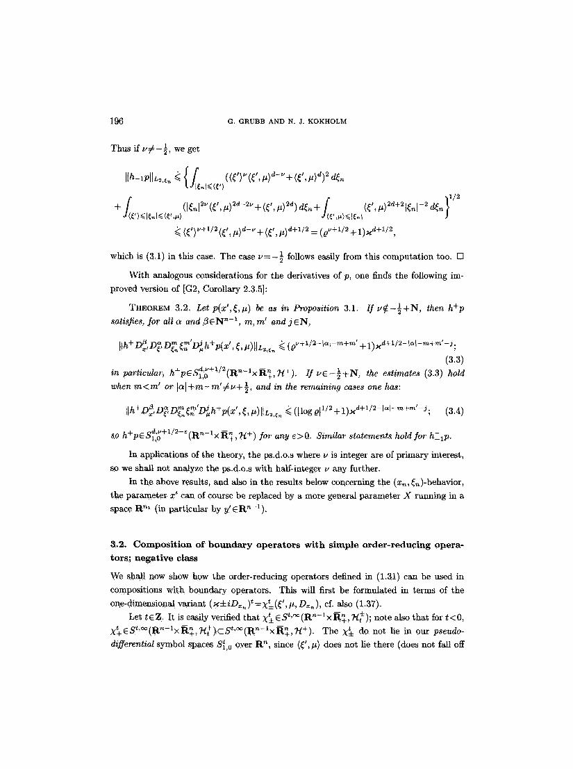
196 G. GRUBB AND N. J. KOKHOLM
v 1 Thus if r we get
+
(~,)v+1/2(~, , # ) d - v + (~t p ) d + l / 2 = (Qv+l/2 + l)avd+l/2
which is (3,1) in this case. The case v = - � 8 9 follows easily from this computation too. []
With analogous considerations for the derivatives of p, one finds the following im-
proved version of [G2, Corollary 2.3,5]:
THEOREM 3 2. Let p(x~,~,#) be as in Proposition 3.1. I f v ~ - � 8 9 then h+p
satisfies, for atl a and ~ E N '~-1, m, m' and j E N ,
t �9 I r t �9 + D ~ a m m ~ + )lh X,Dr162 n Dhh p(x ,~,l.t)llt2,en ~ (p~'+l/2--t~t--m+m +l)>rd+l/2--1,~l--m+~ --~;
(3.3) in particular, h + p E S ~ + ! / 2 ( R = - l x R ~ , ?-l+). I f v E - � 8 9 the estimates (3.3) hold
when m < m t or lal+m-m'#~+�89 and in the remaining cases one has:
h + ~ ~ ,~ m + ~(l logol~/U+l)~d+l/2-1~l-m+m-~; (3.4)
so h§ itS_, 7-I +) for any e>0. Similar statements hold for h-~p.
tn applications of the theory, the ps.d.o.s where v is integer are of primary interest,
so. we shall not analyze the ps.d.o.s with half-integer v any further.
tn the above results, and also in the results below concerning the (xn, ~u)-behavior,
the parameter x" cax~ of course be replaced by a more general parameter X running in a
space R TM (in particular by y'~R~-~).
a.2. Composition of houndary operators with simple order-reducing opera- tora~ negative class
We sh~-t now show how the order-reducing operators defined in (1.3t) can be used in
compositions with boundary operators. This will first be formulated in terms of the
one.dimensional variant ( x • i D=, )t = X~ ( ~', #, D~. ), cf. also (1.37).
Let tEZ. It is: easily verified that x ~ E S t , = ( R ~ - l x F t n 7-/~); note also that for t<0, - § ,
)~t e S t oo{Rn-1 X S t '~176 n 7-l+). The X~= do not lie in our pseudo-
differential symbol spaces S~,0 over R n, since (~', p) does not lie there (does not fall off

A GLOBAL CALCULUS 197
in the (,,,direction when derived w.r.t, (t); so a composition of our ps.d,o.s with Op(Xt, )
will generally !end outside of our ps.d.o, classes. However, the crucial observation we
shall make now is that the X~: do satisfy, not only the L2 estimates for boundary symbol
classes derived in [G2, Lemma 2.3.9], but also the sup norm estimates that were shown
to be valid for decompositions of pseudodifferential $1,0 symbols with the transmission
property in [G2, Theorem 2.2.5]:
LEMMA 3.3. Let tEZ. For any o4EN n, k and jEN,
~ k ~ . ~ l N ' t s , t k ~ ~ , .
O~l<~t-t-k--lo~l--j
where Is~,k,~,j [ ~. (~', #)t-z+k-1':,1-3 (3.5)
k a j t " , t + l + k - ~ - j - 1
Proof. For t~>0, there is no h-1 part, and the estimates of the coefficients s~,k,~,j
are straightforward to see. When t < 0, we write the functions ~nD~k ~Du((~ , j ~ #)4-z~n)" t as
sums of terms of the form
et t/3~ j~ t "~ ~ ( ~ , , , t '~ l ,,-,~' ~",~, , t " , , . , , ~t ~ or c ~ # k~,/~] kk~,#]• ,
where f,l>~O, Ifl'[+f +t '+l=t+k-[(~[- j , resp.
j">~O, t'" <O, I~f ' l+j"+t"+t" '=t+k-Ial- j;
these terms obviously satisfy the desired estimates. It is used here that terms containing m , (~ (({ , #)4- i~)S with m > 0 > s can be reduced away by insertion of formulas
~m = (:t:i)m({~,, # ) . + i ~ _ (~,, #))m : Z Cm,m' ((~', #):t:i~n) m' (~', ~)m--m'. ,~,
(The estimates of the Sl,k,~,j follow also from [G2, Lemma 2.3.9].) []
This leads to the following results on products:
LEMMA 3.4. Let t and t' EZ, and let tEN. (1) W h e n k ( z ' , ~ , # ) e S f ~ o l ' ~ ( R ~ - l x f : t P r , 7 - l + ) , t h e n
dTt-- l , • n--1 h+(x~k(x',r e $1, 0 ( R x R-_~, ~~I-) . ( 3 . 6 )
(2) When t (x ' , ~, . ) esd ;~ (P~n- I xR .~ , ~1~7_1) , then
! ' c Q d + t ' b'(l:: ln--lx'~n "!4-- ~ (3.7) h - ( t (x , ~, ]z)X~) ~ ~ t*r *~'+, ' ~[r+t']+-lJ"

198 G. G R U B B AND N. J. K O K H O L M
(3) When g(x', ~, ~n, P ) � 9 Sd,ol'V(R n- ix R~-, ~-~+~'~r--1), then (with all combinations
of choices of + and - for -4-)
+ - - t ! ' ! ~ o d + t + t ' - - l , v l D n - - I . ~ n d L 4 + ~ q Z - - h~ .hv . (X• ,~,TIn,#)Xt~(~ ,7/'~,#))=~ ~'" ^ " + , ' ~ ~'~[r+t']+-l'" (3.s)
The projections h + and h - can be omitted when Xt~ is taken as Xt+ with t <~O and t ~ t ~ ~• is taken as X-; then moreover, the indication 7-l + vesp. T/~r+t,]+_l can be replaced by
?-l + resp. ?-l~+t, 1.
Proof. This is seen by carrying out the proof of [G2, Lemmas 2.6.2 and 2.6.3] with
X~: (~, #) playing the role of p there, using the estimates from Lemma 3.3 above, followed
by an application of [G2, Lemmas 2.3.9 and 2.3.10]. []
The lemma implies that the full operators Kg=OPK(k) , Tt,=OPT(t ) and G , =
OPG(g), by composition with operators =t to the left and right in a similar way, ~ •
give Poisson, trace resp. singular Green operators belonging to our calculus and having
the same regularity. This is seen first for the cases where K , is given in y'-form, Tg is
given in x'-form, and Gg is given in y'-form resp. x'-form for compositions with =t ~ •
to the left resp. to the right of G, only. In each of these cases it follows from the operator
definition that the full symbol of the resulting operator equals the projected product in
formulas (3.6)-(3.8), without further terms. For more general symbols, we get the result
by changing from x'-form to y'-form or vice versa (cf. (2.26) and [G2, Theorem 2.4.6]);
in the treatment of Gg, one composes first on one side and afterwards on the other side
using these techniques.
Let us also observe that for tER, the operators OP ( (~ ' , g ) t )=(D ' , g ) t, although
they are not ps.d.o.s with symbol in Sst,0(RnxR n+l~ + j, compose very well with Poisson
operators, trace operators and s.g.o.s. More precisely, the restrictions OP((~', #) t )+=
(D', #)~_ = r + (D', #>re + are wen-defined on S (R~) since the (D', #)t preserve the property
of being supported in R~ (but their mapping properties in H~" (R~) spaces are not
convenient for t<0). Now, when T~ =OPT(t(x ' , ~, #)) and G, =OPG(g(x' , ~, 7/,~, #)) are
of order d, class r and regularity u, then a direct calculation shows that
P t T , ( D , #)+ = OPT(t(x', ~, #)(~', #)t), (3.9)
t t G, (D, #) + = OPG(g(x', ~, '1~, #) (~', #>t);
these are operators belonging to the calculus, of order d-f-t, class r and regularity v.
(D', #)~_G, and (P' , #)~Kg are likewise of order d+t and regularity v when G, and Kg
are given of order d and regularity v, with slightly more complicated symbol formulas.
Before collecting all this in a theorem, let us extend the results to operators of
negative class (cf. Definition 2.2 (2)-(3) and (2.36)). Note that one has for any r e Z ,
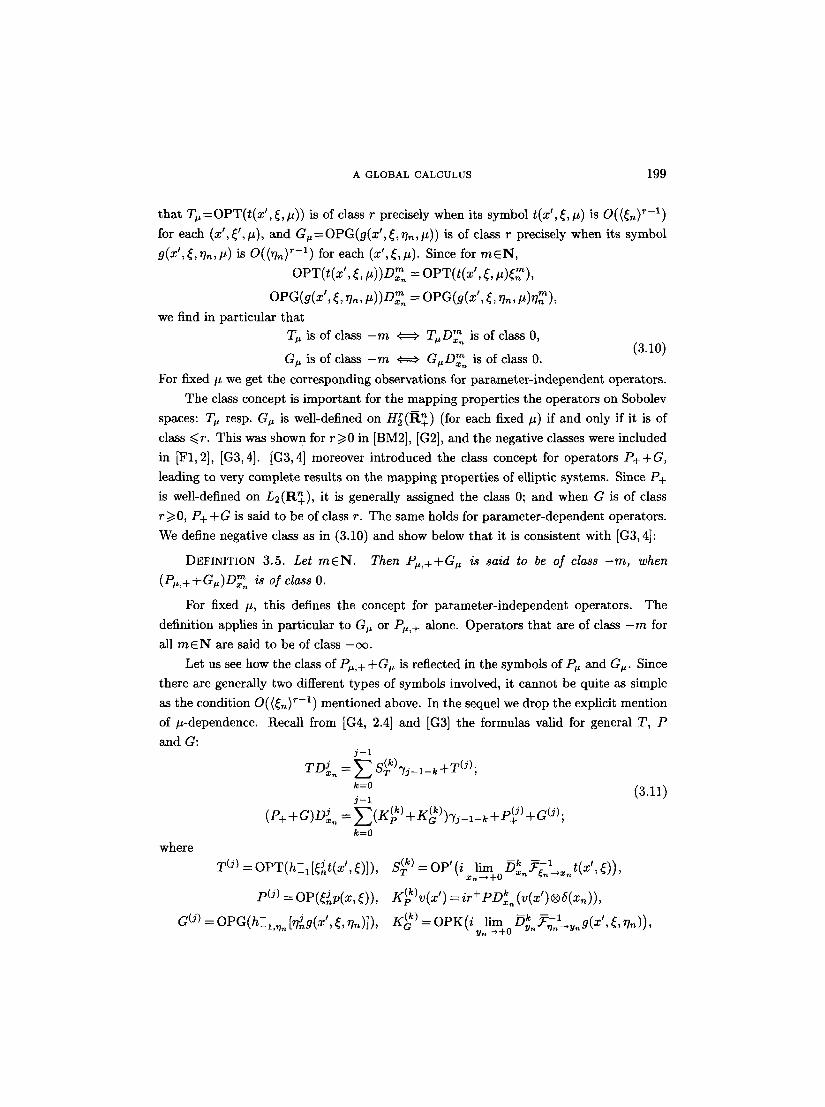
A GLOBAL CALCULUS 199
that T~=OPT(t(x' , ~, #)) is of class r precisely when its symbol t(x', ~, #) is O((~n} r - l )
for each (x t, ~', #), and G~=OPG(g(x',~, ~/,~, #)) is of class r precisely when its symbol
g(x',{,rb~,#) is O((rb~) ~-1) for each (x ' ,{ ,#) . Since for m e N ,
OPT(t(x ' , {, #))D~ m = OPT(t(x ' , {, #){~) ,
OPG(g(x' , {, r/,~, #))D= m = OPG(g(x' , ~, r/., #)rlm),
we find in particular that T, is of class - m r T ,D~. is of class 0,
(3.m) Gu is of class - m ~==:> G~,D,~ is of class O.
For fixed/z we get the corresponding observations for parameter-independent operators.
The class concept is important for the mapping properties the operators on Sobolev
spaces: T u resp. G~ is well-defined on H~(R~_) (for each fixed #) if and only if it is of
class ~<r. This was shown for r/>0 in [BM2], [G2], and the negative classes were included
in [F1,2], [G3, 4]. [G3, 4] moreover introduced the class concept for operators P++G,
leading to very complete results on the mapping properties of elliptic systems. Since P+
is well-defined on Lz(R+),n it is generally assigned the class 0; and when G is of class
r/> 0, P+ + G is said to be of class r. The same holds for parameter-dependent operators.
We define negative class as in (3.10) and show below that it is consistent with [G3, 4]:
DEFINITION 3.5. Let m E N . Then P~,+ +G, is said to be of class - m , when
(P~,+ +G~)D~ is of class O.
For fixed #, this defines the concept for parameter-independent operators. The
definition applies in particular to G~ or Pro+ alone. Operators that are of class - m for
all m E N are said to be of class -c~ .
Let us see how the class of Pro+ +G# is reflected in the symbols of P , and G~. Since
there are generally two different types of symbols involved, it cannot be quite as simple
as the condition O ( ( ~ ) ~-1) mentioned above. In the sequel we drop the explicit mention
Recall from [G4, 2.4] and [G3] the formulas valid for general T, P of #-dependence.
and G: j--1
T D J n = ~ S(Tk)"~j-l-k ..~-T(J);
k=O
j - 1
(P+ +G)DJ~ = ~-~(K~) + K (k)' , + p(+J) +a(J) �9 G } l j - l - k k=0
where
T 0) = O P T ( h - 1 [~Jnt(x', ~)]),
p(J) = OP({anp(x, ~)),
G (j) = OPG(h_-lm" [~(~g(x', ~, rb~)]),
(3.n)
= oP' ( i lira S - : k e)), Xn'*4-O n e,n Xn
K(,,%(x ') = ir+ p n L (,,(x') |
K (k) =OPK( iu~moDk~;s~u .g (x ' ,~ ,~? , ) ) ,

200 G. GRUBB AND N. J. KOKHOLM
cf. (2.1). We see from the first line in (3.11) that TD'~ = O P T ( t ) D m is of class 0 if and
only if S (~ . . . . . S(T m-l) =0; and that when this holds, TD~. is of class 0 for j = 0 , ..., m - 2
also (the latter properties need not be mentioned explicitly in the condition for T being
of class - m , as in [G3, 4]). It then follows also that TD~ ~ ~' =TD~= D~, is of class 0 for
In] ~m, since D ~ does not interfere with the class. The analogous considerations apply
to P++G. Then we find altogether, for m E N ,
T is of class - m -: :. S(T ~ . . . . =S(T m-l) = 0
< :. TD~ is of class 0 for all ]a[ ~< m; /C(0) .1_/C(0) (m--l) (m--l) P+ + G is of class - m -.' " ~ P ~ ~ ~ G ', . . . . . . K p -5 K G = 0
(P++G)D~ is of class 0 for all ]a[ ~<m.
(3.n)
Let us moreover note that in view of (3.10) and (3.12) one has for any rEZ, that T. )-G = - r is of class r -: :- u__,~,+ u__,u,+ T = - r is of class 0; and G . is of class r -' is of class 0.
For P.,+ +Gu one can show that it is of class r if and only if its composition with A-F.,+
(cf. Remark 1.4) is of class 0.
We recall from [G3, Theorem 3.10] that when an operator is of class r for some r 6 Z, 8 - - n then it is defined on Hp(R+) and Bp(R~_) for s > r + ~ - l , but it cannot be well-defined
HS(ftn ~ ~ - n 1 By(R+) for an unless it is actually of class r - 1 . on p~ + j o r s ~ r + ~ - I
Now we can sum up the results on compositions with .-t and (D',#)t: ~ : k , . , +
THEOREM 3.6. Let K , , T~, and G~, be Poisson, trace and singular Green operators
of order d 6 R , regularity u 6 R and class r 6 Z (for T , and Gu), and let t and t ' 6 Z .
When r=O, then =t -+,u,+K u is a Poisson operator of order d+t and regularity v,
TuE~,,,+ is a trace operator of order d+t', regularity u and class [ t '+1 ]+-1 , and
=~ G =t' is a singular Green operator of order d+t+t ' , regularity u and class , . ,+ # ~ •
[ t '+1]+-1 (with all combinations of choices of + o r - / o r +). ~t I "~t' When r 6 Z , T,-_ ,u ,+ and E~,u,+ Gu ~_,u,+ are trace resp. singular Green operators
of order d+t' resp. d+t+t ' , regularity u and class r+t' .
' ~ "D' "~ G and G,(D',#)~_ are trace, Pois- F o r a n y s 6 R , T , (D ,#)+, (D',#)~+Ku, ( ,#)+ .
son resp. singular Green operators of order d+s, regularity u and class r.
The symbols are determined by the usual formulas for composition of the operators
with ps. d. o. s.
3.3. Symbol-kernel estimates in H~'~'(R.+) and L 2 ( R + , x~) spaces
When t is not integer, the symbols X~= are not in 7-/(although they do have the property of
extending holomorpically for Im ~n <0 resp. Im ~n > 0). Nevertheless, we can obtain some

A GLOBAL CALCULUS 201
special results concerning application of (x-iDx~)t+ to the symbol-kernels (recall Defini-
tion 2.2 (5)), that show how some compositions with =t have good properties�9 This ~ - - , ~ , +
implies estimates of the corresponding boundary symbol operators in H2t'"(R+) spaces,
which will be useful in the study of Lp estimates later. The estimates are convenient
since there is no loss of regularity when one applies D = .
THEOREM 3�9149 Let d and vER, let t , t ~ and t 'ER.+, and let h E N n-1. When
Q d - - l , v ( l ~ n - - 1 . ~ n ,t~+~ p k ( X t , ( , . ) e ~ . l , 0 ~,=~. x l r t + , n ) and g ( x , ~ , ~ n , . ) e s d ; l ' v ( R n - l x R ~ , n + @ ' ~ - ~ = l ) ,
then the associated symbol-kernels and boundary symbol operators satisfy:
la[ a �9 t' - I t
= II OPK,~(<~) De,(x-,D..)+k)llz(c,G,.(rt+)) (3.13)
.~ ( ~ + 1)xd+t+e- 1/2; i i i !
�9 t ' D t t l ~ I ~ ~ �9 t - II(x-zD=.)+(x-z y.)+ ( ( ) O~,( -~D~. )+9(x , yn , ( ,#)IIL2 .... ,.(a2++)
(0 ~ + 1)xd+t+t' +t"-l/2; (3.14)
I I ~ l a �9 t ' II OPG~((~ ) Dr163 )
4 (0~ + 1),~ ~+~+~'+~''-'/~. (3.15) �9 t I (3.14) ~nd (3.~5) hold ~l~o ~th (,~-~D,~ ,~p~ccd by (~-~D,~
Proof�9 Consider (3.13) in the case a=0. The operator OPK,~(k): C--*S(R+) acts
simply as multiplication of vEC by the symbol-kernel k(x~,x,~,~P,#); it is also called
OPK~(k), and the application of (x- iD=,) t+ to k corresponds to composition of
(x - iD~, ) t+ with OPEn(k). (We recall that k=:F~-~, k is in e+S(R+) as a function
of x,~, usually identified with its restriction to {x,~>0}.) Hence, in view of (1�9 and
(1.37),
�9 t ~ , t ~ ~ II (,~-~D=.)+ OPK,dk)vll G , ~ ( n + ) = II (x-~D:.)~+ kltL:(R+)IVl = Ilkll H~+,',~(a+)Ivh
and we may assume that t~=0. The symbol estimates for 1r show that for all mEN,
liklIHF.~(~+) = }l(x--iD~,)'~k]]L:(rt+) ~ (0~+l )x a+~-1/2.
Applying this with some m > t and with m replaced by 0, we find by a simple interpolation,
taking 1 - O = t / m (cf. (1.17)):
tiitl.:,~(u+) 4 Itill~:d ~(~.)llitt~o,~(~+) ~. ((o~ + 1)~d+m-~/~)~/m((0 ~ + 1)~d-~/~)l-~/'~ < (0~ + 1)~+~-~/~,

202 G. GRUBB AND N. J. KOKHOLM
showing (3.13) in this case. For lal--1, say c~=(1, 0, ..., 0), we note that
(~'} D~ [r+ (x-iD~)t 'e+ k(x ', x~, ~', #)]
= {~r + OP~(t'(g-i~)t'-lD~,x)e+k+(~'}(x-iD~)~D~,k
= (~')t'(De~)(~-iD~.)e(~-iD,,)+lk+(~')(~-iD~.)+De, k,
cf. (1.34). The latter two expressions are similar to those we have already treated, for
(x- iD~)+l~ is a Poisson symbol-kernel of order d - 1 and regularity v:
~ - ~ . r + ( x - iDz . ) - l e+ Ic= h +[(~-i~n)-l k(x',~, #)] e S d-2 , v ( R n - 1 )~ l_L+, ~ . ~ + ) . ~ n
by Lemma 3.4, and D~j k is a Poisson symbol-kernel of order d - 1 and regularity v - 1 ;
moreover, the factor (~')Dr >r is ~ (~'). Since one has in general (cf. (2.1))
((')l-I(e~-I-I + 1)~--I-I ~ (e~+ 1 )x ' , (3.16)
we conclude that (3.13) holds for a= (1 , 0, ..., 0). The general estimate (3.13) follows by
iteration of this argument.
The proof of (3.14) is very similar. Again we begin with the case a = 0 , and use
that (g-iD~,)t+(x-iD~,)~ equals (x-iD~)~+ +t', so we may assume t'=O. In view of
the symbol rules, we only have to account for the cases where t and t" E [0, 1]. Here we
depart from the inequalities, valid by the definition of S d-l,",
II~(~',~,y~,~',~)IIL~ .... ~o(R~+)~(~+I)~ d,
II(----iO~,~)~llL~(R~+)+ll(x--iOu.)~llL~(rt~+ ) ~ (Q" + 1)x d+x, (3.17) II(x-iD~,)(x-iny,)~l[i~(a~++) ~ ( e ~ + l ) x d+2,
which show (3.14) for t and t" equal to 0 or 1 (and t'=O, a=0) . Since one has for
functions f : R + - + X when X is a Hilbert space,
II(x--iD~,~)~f(xn)llL=(a+;X) = IIf(xn)llHg'"(~+;X),
we can read the statements in (3.17) as Sobolev space estimates of vector valued functions.
Then we obtain (3.14) (with t '=0 , c~=0) by application of interpolation, first between
the spaces L2,z~(R+;Y) and H21'"(R+;Y), with Y equal to L2,y~(R+) or H~ '" (R+) ,
and thereafter between the spaces n2,v~(R+; X) and H~'"(R.+; X) with X=Ht'"(rt+). The factors (~')I~1D~, are included in a similar way as for/r by use of the Leibniz formula
and Lemma 3.4.
For the explanation of (3.15), we let (~---0; the general case can afterwards be included
by a calculation using the Leibniz formula. Then we can also assume that t'=O. The

A GLOBAL CALCULUS 203
estimates (3.14) can be read as Hilbert-Schmidt norm estimates of the family of operators
OPG.(g') from L2(R+) to L2(R+) (parametrized by (x', ~', #)) with the integral operator
kernels
~l[X! 32 g t , n ,Yn ,~ ' ,# ) ( x - iD=, , ) t+ (u - iDy . )~ 'O(x ' , xn ,Yn ,~ ' , / z ) .
One has a fortiori that the operator norms of OPG,~(g') in s axe
bounded with the same bound as in (3.14). This carries over to Sobolev space estimates
of OPGn(g) itself, as follows: Let uEH~;~"'"(R.+) and set v = ( x + i D = , ) - t " f i . In view of
(1.34), v identifies with a function in L2(R+), and moreover, by duality,
/o ( x - iD=. ) t+ OPGn(g)u ( x - i D ~ . ) t + - ' x ' �9 t,, = g ( x , . , y . , ~ , # ) ( x + , D v . ) v (yn)dyn
~0 ~ " t . ~,t~ ~ ! = [ ( x - t D = . ) + ( ~ - ~ D u . ) + g ( x , x . , y n , ~ ' , # ) l ~ ( Y , O d y .
= OPG.(g')~.
Then the L2 operator norm estimates of OPG.(g') imply
,, " u d+t+t" II OPG~(g)II~:~H-, ,"'K ' H ' " K " ~< (0 +1);~ . t 2;0 k +), 2 I. +))
(3.1s)
For the last assertion, one uses that the adjoint OPGn(~(x', x . , yn, ~', #))* equals
OPG.(~(x', y. , x. , ~', #)), which is of the same kind as above. []
We shall also need to analyze the effect of multiplication of the symbol-kernels by a
fractional power of xn, or rather, the study of the norms of boundary symbol operators
in L2(R+, x~n) spaces, cf. (1.46). This is more delicate than the preceding study, since
the multiplication by xn lowers the regularity by 1, and the regularity concept does not
always interpolate well.
Let k(x ' , ~, ~)Esd- l 'U(Rn-lx R_~, "1-~+); then k(x, ~', ~t) satisfies, by definition,
II~:[IL~,=.(R+) ~ (0 "+ I )x a-1/2, I[x,~k[[L~,=.(R+) ~ (8~'-1+1)x a-3/2. (3.19)
Let 0< 6 < 1, and recall the interpolation inequality
6 X 1-6 X 6 ]lXnf( n)][L2(R+) ~ IIf(Xn)HL2(R+)]]Xnf( n)HL2(R+); ( 3 . 2 0 )
it gives for k:
u 1 6 u 1 6 d 1/2 6 HkllL~,. IIx.kll~.~,=. ~(Q + 1 ) - (Q - + 1 ) x - - (3.21)
<~ (1 + 0 ~'(1 -~) + 0 (~'- 1)~ + 0,,-~)>~,~- 1/2-~.
14--935204 dcta Mathematica 171. Imprim6 le 2 f~vtier 1994

204 G, GRUBB AND N, J. KOKHOLM
Here m i n { v ( 1 - ~ ) , ( v - 1 ) & v - 6 } = v - ~ f if v < 0 and is >/0 if v~>l, so that (3.21) implies
(recall that p ~ + 1 - 1 when a~>0, cf. (2.1))
t]x~n]~ltL2.~ ~ ( ~ - ~ + 1)x d-1/2-~ when v e R \ ]0, 1[; (3.22)
which is as good as one could hope for; note that u and L,-6 have the same sign. But
when ~ ]0, !~, we only get
]IX~HL2,= n ~ (g~L,-6 _~_ 1)xd-1 /2-~f , V E ]0, 1[, (3.23)
where S v - 6 = v - ~ - ( 1 - 6 ) v is <0 and < v - & Note however that (3.21) is fine in the
region 1~'[ >~(#), for here (~'),.~ (~', H), so (3.21) is equivalent with
llzZ ll =,=. r z when ]~'t >/(H). (3.24)
~ e n n > l (the case of principal interest for applications), we can use (3.24) together
with a consideration of derivatives to extend (3.22) to all v r with just a logarithmic
loss when v=6. The proof is given in the following theorem, where we also collect facts
shown above.
THEOREM 3.8. Let d and ~ER, 6E]0, 1[, a E N '~-~, and assume that n > l if v~
]0, 11 . Let k(x',~,H) be a Poisson symbol in Sd-"~'(R~'-'xf{.~_,'tt+). Then
i,x~,.,, ~ Da[c" , . , { ( ~ - ~ + 1 ) ~ -~/~-~ when v r (3.25) ' ( l logel ' /2+l)~ -1/=-~ when ~,=5.
Proof. Consider first the case a = 0 . The result is proved above when u E R \ ] 0 , 1[,
so we let vE ]0, 1[. For ]~']~>(H) we have (3.24) which shows the desired estimate in that
region; it remains to consider I~ r] < (H)- Let ~ '#0, then the basic trick is to integrate the
following inequalities along the ray in ~'-space from ~' to ((#)/]~r])~,, using (3.24) at one
endpoint. For l<~j<~n-1 we have (with norms in L2,=,(R+)):
5 ID~ IIx~.~:lt 2 ] 42 x~]k(x,~',#)D~jk(x,~',H)ldxn (3.26)
<211xJcllllx~-~D~jkll for 6~ 1
ID~llx~klt~l <211x~%1111D~kll for 6 > 0 . (3.27)
First we treat the values v,6 with 5>v. Here we prove by induction on I that for
l=O, 1, ...,lo, where 2-1~ <L,,
[]x~[r ~. ( Q " - a + l ) x d-1/2-a, when 6 > u and 2 -1-1 < 6 < 2 -t . (3.28)

A GLOBAL CALCULUS 205
The induction start is based on (3.26). When �89 then 0~<2b- l< l and we can
apply (3.22) (with ~, and b replaced by v - 1 and 2b-1) to the second factor in (3.26),
which gives
I Dr IIx Yr k + + ~02v--26--1X 2d-2-25 ;
in the last inequality we used that b>~u. ]t follows that
IIx tl = k x2d-1-25-b f(/z)(t> 2v-25-1 (/~>2d-2v-1 dt Jlr
k (~ l }2u -2g( I .~ )2d - l -2 r ' J f - ( / .~}2d-1 -25 k (~Ov-~iJ'cd-1/2-lY) 2, (3.29)
which proves (3.28) for/--0. Since k is smooth and the estimate is uniform in (~', #) for
~'r it extends to all (~',#) ERY+. Now we have when b>u and 2-q'+1)-1 ~<b<2-q'+l)
that 2b>u and 2 -(z'+~) <~.2b<2 -z'. So if (3.28) is proved for l=l', (3.29) gives
IDr IIx ll [ ~ ~'-2~fxd-1/2-21f~ v-11"~d-3/2 k ~ 02t~-2tf-lx2d-2-2~, (3.30)
and then (3.28) follows for l= l '+l by integration. By induction (up to l=Io), (3.25)
is obtained for any b>u. An inspection of the proof shows that the case b--u can be
included, giving (3.25), when the estimate of the integral in (3.29) is replaced by a
logarithmic estimate.
Finally, the values b<u are treated as follows: If 0 < u / 2 < b < # , then 2b>u and
2 u - 2 ~ i - 1 > - 1 , hence (3.30) holds and gives (3.25) by integration. The remaining bE
]0, u/2] can be included by interpolation of the estimates for b=0 and b=3u/4, much as
in (3.20) ft.
When a~0 , (~')laID~,[r is of order d and regularity min{u, ]aI} (cf. [G2, Lemma
2.1.6]), so the preceding result applied to (~'}l~lD~,[r implies (3.25). []
Note that the trick in Theorem 3.8 also improves [G2, (2.2.90)] when n > l .
We shall now consider singular Green symbols. Here one can study the effect of mul-
tiplication of the symbol-kernel with x~ as well as y~, corresponding to letting OPGn (g)
end in or start in a weighted L2 space over It+. What we shall need later is a mixture
of this with the applications of (x-inz~)t+ and ({')I-ID~, studied in Theorem 3.7, and
we go directly to the needed result. Recall the notation (1.46).
THEOREM 3.9. Let d and uER, bE [0, 1], t and t' E~l~+, a E N n-l , and assume that t d l v n l n n > l ifuE]O, 1[. Let g(x ,~,~7~,#)ES - ' (R - xR+,7-/+@7-/_-l). Then the associated

206 G. GRUBB AND N. J. K O K H O L M
symbol-kernel 9(x', xn, yn, ~', #) satisfies:
Iix~(x_iD~,)t+ , I~l ~ �9 t'~ <~ ) Dr .... , ,(R~+) and
Hy~(~-iD=,~)t+(~ )lalD~,(x--zDz.)t+gHL2 . . . . v,~(R~_+ ) are
{ (Qv-5-4-1)xd-5+t+t' when v#5 , or S=O or1;
(llogvll/2+l)x d-~+t+t' when v=~iE]0 ,1[ .
(3.31)
The operator OPGn(g') with symbol-kernel ~ '=/ r I,~ID2 ( x i D = ~t' ~l satisfies:
H OPG~(g')IIL(H~,x(K+),L~(R+,=~)) and II OPG~(g')H~(L2(R+,=~),H~'X(~+)) are
.~ f (~)~-~+1)~ d-~+~ whenu#~f, or~f---O or1;
(llog ~lz/2q-1)~ "d-6+~ when u = $ E ]0, 1[.
(3.32)
Proof. Consider the estimate of the first norm in (3.31). Since xn~ is of order d - 1
and regularity v - l , it follows from Theorem 3.7 and considerations like (3.11) that the
estimate is valid when ~i is 0 or 1. Then we apply a version of the preceding considerations
on ~c (the interpolation in (3.20) and the lifting from lower regularities in the proof of
Theorem 3.8), now for vector valued functions. This gives the estimate of the first norm
in (3.31), and the estimate of the first norm in (3.32) follows from this as in the passage
from (3.14) to (3.15) in Theorem 3.7.
For the estimate of the second norm in (3.31), we just have to interchange the roles
of xn and yn, then the estimate of the second norm in (3.32) follows by variant of the
explanation in Theorem 3.7, where we use the duality (1.47). []
Remark 3.10. We shall not burden the exposition with more detailed conclusions
based on (3.23) for u e ]0, 1[ and n=l , that can be worked out when needed. Instead, let
us mention another technique giving adequate resolvent estimates:
In the resolvent construction for normal elliptic boundary problems, the symbols of
the boundary operators are of integer or half-integer regularity (cf. [G2, 3.3]), so it is
only symbols of regularity �89 that axe not covered by (3.22). But here one has additioi ~1
information, namely e.g. that the Poisson symbol-kernels of regularity �89 and order d
satisfy estimates
II(Lx,+)~k(x',x,~,~',#))IL~,(R+) ~ x d-1/2, for ~ie [0, �89 (3.33)
where L,,,+ is the Laguerre operator on R+, L,,,+=-x-lO=.xnO=, + x x , ~ + l . We recall
from [G2, (2.2.15)] that IIL~,+IClIL2(R+) is equivalent to the g2 norm of the Laguerre

A GLOBAL CALCULUS 207
expansion of/r Estimates like (3.33) hold both for the terms in the direct operator .At,,�9 and its inverse B,,e; see [G2, Remark 2.6.16, Theorems 3.2.3 3 ~ and 3.3.1]. Now
(L>,,+u, ~t)L2(R+) ~- 24 - 1 ( X n O x . U , Ox,~U)"}-24(XnU, ?.t)-}-II~t]] 2,
for u � 9 since 7o(X,~O~u)=0. The terms are/>0, so one gets the operator inequality
L,~,+ > / x x , + l , in the sense that (L,,,+) -1 ~< ( x x n + l ) -1.
By an operator-theoretic monotonicity theorem (cf. e.g. Donoghue [D]), this implies
(n , , ,+ ) -~<(xxn+l ) -~ for a6]0, 1[, and hence, by (3.33),
IJ (xx,~ + 1)~: H L 2 (1%+) --~-- ( (XXn -{- 1) 2~:, ~:) 1/2 (3.34)
< k)1/2 = ijLi+ ll < 24d-1/2, for �9 [O, 1[.
Thus (3.25) holds for ~6 [0, �89 [ and n=l also, in this case. Similar estimates hold for the trace symbol-kernels of class 0 entering in the resolvent construction. The arguments
likewise apply to the singular Green symbol-kernels ~ entering into the resolvent con- 1 struction, of class 0, regularity ~ and order d, say. Here one finds by application of the
above method for the xn-vaxiable and straightforward Sobolev space interpolation for the yn-variable:
I I ( x x n + l / ( x - - i D y , , ) t + ' l l L 2 . . . . ,=(a~+) ~< I[(L,,,+/(24--iDy,~)t+gllL2(R~_+) (3.35)
Z d+t for 6 �9 [0, 5
Such estimates hold also with x,, and y,~ interchanged, so (3.31)-(3.32) holds for 66 [0, 1 [ and n = l in this case.
The methods also allow an improvement of [G2, Theorem 2.6.6], concerning the sym- bol g+(p) of the special s.g.o. G+(Pt,)=r+Pue-J (recall that J: u(x', x,~)Hu(x',-x,~)).
THEOREM 3.11. Let p be as in Proposition 3.1, with u ~ - � 8 9 and let n > l if u>-�89 If uCN, then [t+(p) satisfies for all indices a , ~ � 9 n-l, k, k ' ,m,m' , jEN:
I t , ! [3 o~ k k m m j ~ + I I]D~,Dr n y n , g (p)(x ,x,~,y,~,~ ,#) L2 . . . . un(R~_+) (3.36)
( @ u - l a l - k + k ' - m + m ' + 1 ) 2 4 d - l a l - k + k ' - m + m ' - j ;
in particular, g+(p) belongs to sd-I,~(R'~-lxR~_,T/+@T/_-t).
If u �9 (3.36) holds for all indices except those satisfying
k>~k', m ~ m ' , l a l + k - k ' + m - m ' = u , (3.37)

208 G. G R U B B A N D N. J . K O K H O L M
for which one has
a k k' m m' j -+ t IIPx, D~,xnD~,~yn Dy,~ Dt, g (p)(x ,x,~,yn,r .... ,n(R~+) (3.38)
<~ ([log Qil/2+l)xd--I~l--k+k'--m+m'--J;
SO g+(p)ESd-l,v-~(an-l•163 7-/+@7-/_-1) for any ~>0.
Similar estimates hold for g- (p).
ProoL It is shown in [G2, Theorem 2.6.6] that ~+(p)=(.~(~Lzh+p)l~=x.+u. for
1 Then we get by application x~,y~>0. By Theorem 3.2, the regularity of h+p is v+~.
of (3.25) with 5=�89 to/~+=~'~-Lzoh+p:
(fs ' J'l/ = IP ( .+Y. , r Ilg+(p)(x',xn, yn,~',#)]lL2(R2++) -+ X' X '
= (2 fR+ dz=) (~u+l/2--1/2-~-X)xd - - (Q" + 1 ) , d,
where Q~ is replaced by [log ~[1/2 if u=0. In a similar way, we get improvements of the
estimates in [G2, Theorem 2.6.6] of the derived symbols. For example we have, since
D~.p is of order d - 1 and regularity v - 1:
IIXng+(p)(x/'Xn'Yn'~/'")IILz(R2++) ~ ( f R (Xn-~-yn)21p+(xt'Xn-~-Yn'~t'")12 dxndyn) 1/2
= ( 2 JR+ Z.W I oh + ( Dr dz@ 1/2 (ev-1+1/2-1/2 + 1)xd-1 = (Q~-I + 1).d--l,
with Q~-~ replaced by Ilog011/2 if u = l . - - The result for g-(p) follows since g - (p )= g+(p*)*. []
This result permits an improvement of the regularity numbers in the general para-
metrix construction from [G2, 3.2], see [G5].
Remark 3.12. The logarithmic loss in case uEN in Theorem 3.11 can be removed
in some special cases, for example when p is a rational function of ~ and # of the form
(f(x',~)g(x~,~)-i+#l) -1 with f and g polynomial in ~ of degree k+l resp. k (here k
and 1EN, and d=-l) . The proof is somewhat long, and will be left out since it is
not necessary for the resolvent estimates taken up [G5], where the loss of regularity is
eliminated by other methods established in [G2].

A GLOBAL CALCULUS 209
Remark 3.13. Let us note that when v=0, and d=0, say, then the L2(R+) operator
norm of OPG~ (g+ (p)) is .~ 1 (without a logarithmic loss), simply because the operator
equals r + OPn(p )e -J , where the L2(R) operator norm of OPt(p) is ~1. One can extend
this to uniform bounds in f..(H~ (R+),H~ (R+)) and s by
use of formulas such as (4.25) below and a related version containing the multiplication
by x,~. But these estimates are far from the generality covered by Theorem 3.9, and we do
not see how to obtain the estimates in Theorem 3.9 for g+(p) with general independent
values of 5, t and t' (or just those values that enter in the proof of Theorem 4.1 below)
without using Hilbert-Schmidt norm estimates, such as the estimates of the symbol-
kernel in Theorem 3.11.
4. Lp estimates of parameter-dependent operators
4.1. Es t ima tes on Euclidean space
We shall now extend the L 2 mapping properties shown in [G2, Section 2.5] to Lp spaces,
l<p<c~ . The basic result is the following theorem on mapping properties for operators
with x-uniformly resp. x'-uniformly estimated symbols (cf. Definition 2.1).
THEOREM 4.1. Let d and v E R , let pE ]1, c~[, and let rEZ . d,~ n - - n + l (1) Let p(x,(,g)eS1,0(R xR+ ). Then Pg=OP(p(x ,~ ,# ) ) is continuous for all
sER: P,:H;'~(R'~)--~ H ; - g " ( R '~) and
(4.1) P, :Bp'g(R n)-~B;-d ' t ' (Rn), with norm O({#}-~+1).
(2) Let with n > l il el0,1[ andp<2. Then
Kg=OPK(k) is continuous for all sER:
Kt~:B~-I /P"(R'~-I) --~ r-r~-d't'l~n~ ~'v ~,~+jMB v ~-d,g (R+),-'~
with norm O((#)-~'+[1/P-1/2]+ + 1), (4.2)
i l 1 unless O < v - - ~ - 5 , where the norm is 0((]~) ~) for any ~>0. (3) Let t (x ' ,~ ,# ) d,~ ~-1 --~ - ESI,o(R xR+,?-/~_l) (of class r), with n > l /f rE]0,1[ and
p>2. Then T ~ = O P T ( t ) is continuous for all s > r + l - l :
Tg: H i~'€ (R+) + B y - = ~'g (R+)-~ --* Bp-d-I/v't'(R'~-l), with norm 0 ( ( # ) --~+[1/2--1/pl+ -~- 1),
(4.3)
unless 0<u=�89 1 --~, where the norm is O((p} ~) for any e>0.

210 G. G R U B B AND N. J. K O K H O L M
d~b' n (4) Let p(x,G#)ESLo,utt~(R xR~_+I), with n > l if uE]- �89189 and p<2. Then
Pro+ =OP(p(x, ~, #))+ is continuous for all s> ~ - 1:
P/z,+: s,tt --n Hs-d,u(~n H i (R+)-~ p , +, . .,~, - n ~B;-d,/z(fft~), Pro+" Bp (a+)
and (4.4)
with norm 0( (# ) - "+1) .
(5) Let g(x',~,rl.,#)eSdl~l'v (R"- lxf f~_, 7~+ ~'kl~r_l) (of class r), with n > l if vE
]0,1[ and pr Then G,=OPG(9) is continuous for all s > r + 1 - 1 :
G /z : B;'/z (fft ~_ ) ~ n,-a,/z (U,~
and (4.5)
with norm 0( (#) -~+li/p-t/zl +1),
unless 0 < u = 11 ~-�89 where the norm is O((#)') for any ~>0. Moreover, if P~,,+ is as in
(4) and P,,+ +Gu is of class - m for some m E N , then (4.5) holds with G/z replaced by
P,,+ +Gu, for all s > - m + ~ - l .
(6) Let p(x, ~, #) be as in (4). Then the s.g.o. G+(P/Z) is continuous for all s > 1 y - l :
G+(G): G-d,. and
(4.6) with norm O((#)-~+1).
0,v n - - n + l Proof. (1) We shall apply Theorem 1.6. Since symbols p(x ,G#)ESI ,o (R • )
satisfy (1.44) with C(p)=O((#)-~+l) (H0=Hx=C), the first statement in (4.1) follows
immediately for the case d=s=0 . When s and d are general, one reduces to this case, .qO,u cf. (1.5), by replacing Pu by (D, #)s-dpu(D, #)-s, which is a ps.d.o with symbol in ~t,0,
hence is bounded in Lp(Rn), uniformly in #. The statement for B~ ,# spaces follows by
interpolation, cf. (1.16). This proves (1).
(2) For the boundary operators, results for fixed # were proved in [G3] and [F1, 2];
and we shall to some extent follow [G3] in the argumentation. In view of the for-
mula (2.35), K# can be considered as a vector valued #-dependent ps.d.o. Q(x', D', #)
in the x' variable, such that the symbol takes values in a space of linear mappings
c~->[r ~, xn, ~, #)c from C to a function space over R+. Here [r ~, xn, ~', #) is in S(~.+)
as a function of x~, on which many different norms can be used.
For one thing, 1r satisfies, by hypothesis, the estimates for all c~ and flEN n-1 (recall
that x = (~', #)):
II (C>l t D~,D~, (Ir x . , #)x -d+1/2) + 1,
~' R "-I, i>0, for x', E # (4.7)

A GLOBAL CALCULUS 211
Then since OPz,(;,r d-l/2) is an isometry of Hdp-1/2'~(l:~ n- l ) onto Lp(R n- l ) (cf. (1.5)),
we find by application of Theorem 1.6:
K~:Hd-1/2'~(R'~-I)---*Lp(Rn-1;L2(R+)), with norm O((lz>-~+l). (4.8)
When 2~<p<oo, we also use that
"-'~,~z,~xn (k(x', xn, ~', #)x-d-1/2)II,'(C;L2(R+ ) ) ~ (#)-~ +1,
which gives, by use of Theorem 1.6 and (4.8),
K~,: d+1/2,~ n-1 H; (1t )-~Lp(11~-l 'H~(R+)) , with norm O((#}-~+1).
Using Corollary 1.9 (2) we then find by application of real interpolation (. ,-)l/2-1/p,p (cf. (1.16)) the boundedness of:
K,: Bd-1/P'"(11 '~-1) ~ Lp(11_'~), with norm O((/~)-~+1).
By composition to the left with operators =t t 6 Z (cf. (1.31-34)) we get moreover, ~--,/~,+,
since =t K is a Poisson operator of order d+t and regularity v by Theorem 3.6, ~--,/~,+
K , =-t =t ,I ,-,t+d-1/p,,,,-.n-1, , , t , , ~ n , O((#}-V+l). = n , : D p t*t )--+rip' t , t+), with norm
The mapping property is extended to arbitrary t 6 11 by complex interpolation (cf. (1.28)); and by real interpolation we furthermore get
K~,: ,~t+d-1/p,,,--,~-l, n t ,u ,~n , O((#}-~ + 1). Dp ~*t )--*Z~ v (*t+), with norm
This shows (4.2) for p>~2. When l < p < 2 , we choose a ~6] 1 1 1 y - ~ , ~ [ , $#v, and apply Theorem 1.6 to
k(x', x~, ~', # )x -d-1/2+6, considered as a ps.d.o, symbol in (x', ~') for each/~ with values
in s L2(11+, x~)); it acts as in (4.7) with right hand side O((#)-~+~+1) by Theorem 3.8. This gives
g~, r r d + l / 2 - - 6 , 1 ~ r r [* ' *n - -1 :np t*t ~-~.pt . t ;L2(11+,z~)), with norm O((~u)-~+6+l). (4.9)
Here the interpolation ( . , . )(1/p-1/2)/6, p applied to (4.8) and (4.9) gives, by use of Corol- lary 1.9 (1), (1.16) and (1.17):
K~,: Bd-1/P'"(11 n- l ) ~ Lp(11~_), (4.10)
with norm O(((]z)-~ + 1)1--(1/p-1/2)/6((~)--v+6 "Jr 1)(1/p-1/2)/~).

212 G. G R U B B AND N. J. K O K H O L M
When v~0, this is estimated by
0({#) [vl(1-(1/p-1/2)/l~)+(ivl+5)(1/p-1/2)/5) : O({#)]vI+I/p--I/2), (4.11)
and when ~> ~ - �89 we can take 5<~, getting O(1); this shows the desired result if v~0 1 1 __1 1 or v > ~ - ~ . If ~ - ~ - ~ , we get the estimate O((#) ~) by taking 6 arbitrarily close to
1 1 [, we replace the above interpolation argument by one where v. Finally, if vE ]0, ~ - ~
we interpolate between two versions of (4.9) with 5' resp. 5, where ~<5 '< ~ - �89 <5, and
use (1.50); this gives the desired estimate. Lp(R~) is replaced by H~ 'g spaces and B~,it
spaces in the same way as in the case p~>2; and this completes the proof of (2).
(3) If r~>0, we are dealing with operators and symbols as in (2.37), (2.36). For the
terms Sj,g~j, the result follows from (1.29) and (1). For the term T~ of class 0, the
result follows, for ~ - l < s < ~ , from (2) by duality, using that T~* is a Poisson operator 1 1 1 of order d§ 1 and regularity v; here ~ - �89 is replaced by ~ - ~, since the Poisson operator
• 1 By composition to the right with operators is considered in Lp, spaces with p , - ~. 1 1 =t one gets (4.3) for t + ~ - l < s < t + ~ , tEN, and the exceptional values s E ~ + N are ~ - , # , +
included by complex resp. real interpolation. If r=-m<O (cf. Section 2.2), we can write
- - T ~ m ~ , - m T i t - - tt ~ - , t t , + ~ - , i t , - { - ,
where Tit~m, it,+ is a trace operator of class 0, order d§ and regularity v according
to Theorem 3.6. Then in view of (1.34), the region where (4.3) holds extends down to
s > - m + ~ - l . This proves (3).
(4) Here we use the scheme of [BM1] in the same way as in [G3, Theorem 3.4], so
the explanation can be brief. In view of the formulas
D~ne+u = e+D~, u~=i(~ou)(x')Qh(xn),
Dx~e• = e• for j < n; (4.12)
one has, setting Kuv--r+P~(v(x')|
Dx, Pit,+u = P~,+D~, u+ [Dx,, P~]+u-iKit~/oU,
D~jP~,+u=P~,+D~ju+[D~,P~,]+u, for j <n . (4.13)
K~ is a Poisson operator of order d-t-1, and its regularity is v+ 1 except when ~ E - �89 §
where the regularity of K~ is v+ �89 - c , any e>0; these assertions follow from Theorem 3.2,
when we use that Pt, can be written on (x', yn)-form (cf. (2.29)): P~--OP(q(x ~, Yn, ~, #)),
and then the symbol of Kit equals h+q(x r, O, ~, #). When ~ - l < s < ~ , l 1 (4.4) follows directly from (1) in view of (1.28), first line. Next,
it is proved for t § 2 4 7 1 by induction in t e N using (4.13). Here we apply (2)

A GLOBAL C A L C U L U S 213
to Ko, noting that the norm in the various spaces will be O((/Z) -~-1/2+~+[1/p-1/2]+ + 1),
which is O((/z)-V+l) for small ~. The full range of s, and the generalization to Besov
spaces, is obtained by interpolation as in [G3, Theorem 3.4]�9 This shows (4).
(5) If r>~0, we are considering operators and symbols as in (2�9 (2.36), with G~ of
class 0. The terms Kj,o~ j are handled by (1.29) and (2). The result for a case r=-m<O �9 �9 _ . ~ m ~ - - m is derived from the case r = 0 by writing G o-Go~_,o ,+~_,o ,+ , similarly to the treatment
of T o in the proof of (3); here G ~m is of class 0. Thus we may assume that the class O~-- ,O,+
r is zero.
In view of (2.35), G o can be considered as a vector valued /z-dependent ps.d.o.
Q(x ~, D t,/Z) in the x' variable, with the symbol valued in a space of linear mappings from
a function space over R+ to another, v(x~)~-~(g(x j, ~',/Z, Dn)v)(xn). Here g(3J, ~',/Z, Dn) R2 is an integral operator with kernel 9(x', xn,y,~, ~',/Z) lying in S ( + + ) as a function of
x,~, y,~, so many different norms can be used.
Let p~>2. Consider first the case d=0. Here we have by Theorem 3.9 with t=~,
t ' = 0, that for any ~ e [0, 1] such that 5 ~ u if u E ]0, 1 [, and any a,/3 E N n- 1,
]1 (~')I'~lD'~,D~,g(x', ~', #, Dn)I]s
<<. I[(~')l~'lD~,O~,g(x',r (4.15) ((~')/(~',/z))~-a + 1 ~ (/z)-u+a + 1,
since II ~11 Hg (a§ <~ II ~11 Hg" (~+)" It t hen follows from Theorem 1.6 that G o is continuous
Go: Lp(Rn-1; Lu(R+, x ~ ) ) ~ Lp(Rn-1; H26 (R+)), (4.16)
with norm O((/Z)-~+~+I).
If p=2, we get the continuity of Go:L2(R~)~L2(R'~.), with norm O((/Z)-~+I)
directly from this, taking 5=0. Here in fact the estimates (4.15-16) follow directly from
the symbol properties, and one need not appeal to Theorem 3.9.
Now let p>2. When u r 1 8 9 we use (4.16) with ~=~1 and ~ = ~ satisfying 0~<(51 < 1 1 1 --~ < ~ < 5 and u~ [~, 5~]; then we get by interpolation using Corollary 1.9 that
�9 n n O ( ( / Z ) - v + I / 2 - 1 / P q - 1 ) . ( 4 . 1 7 ) G o. Lp(R+) ~ Lp(R+), with norm
When _ 1 1 v - 7 - ~ , we get the estimates with a loss of e> 0 as in (2).
=-d G which is a s.g.o, of If d is integer r we apply the same treatment to - - ,o ,+ o,
order and class 0, and regularity v, by Theorem 3.6. Then we get in view of (1.34),
m
L n (4.18) Go: p(R+)-~Hp-d '~ w i t h n o r m
O(</z>-~+l /~ - , /p+ l ) for , 1 1 1 ~ r O((/z>~) for ~ = ~ - ~ > 0 . (4.19)

214 G. G R U B B A N D N. J . K O K H O L M
When d is noninteger, -_-d G is not a standard s.g.o., but some formulas can be ~--,#,+ #
used anyway. Assuming as we may that Gu is given in y'-form, Gu---OPG(g(y', ~, ~?n, #)),
we can write
_--u G =t' ~k G - - - t ' G I - G " (4.20)
~k where t'>0, kEZ, G~, is the s.g.o. __ u,+Gu of order d+k, class 0 and regularity u by
Theorem 3.6, and G~ is the generalized s.g.o.
G~=OPG(g")- -OP ," "" ' ~' x Lg LY,~ ,# ,Dn)) , where �9 _ , ,
=(x-,D,~)R+g (y ,xn, Yn,~',#)
~'(y',x~,y~,~',#) = (~<-iD~)k+~l(y',x~,yn,~',#).
Theorem 3.9 applied to g' shows that g"(y', ~', #, D~) satisfies
]l (~')I~1D~ D~,g"(y', ~', #, D~)]]s (4.21)
<~ [{(~ ) Dr (y ,~ ,~,Dn)[{f_.(L,(R+,:~V,~),H~,"(~.+)) { </~) -u+~+l ,
for all 6~[0, 1] with 6 r if u~]0 ,1[ , all a and ~@N n- l , and hence it follows as in the
first part of the proof that
G~: Lp(R~.) ~ Lp(R~) , with norm (4.19).
Then by (4.20), we get (4.18) using (1.34).
We have hereby obtained (4.18)-(4.19) for all dER, when p~>2.
In order to generalize this easily to more general H~ ,~ spaces and to p<2 , we shall
prove an auxiliary result that may be of some independent interest. The result is that
the restriction of G u to r+So(R~) (cf. (1.25)) has a continuous extension
G~:H~;~(~t~)-* H~-d'"(Ft~), for all t e R , l < p < c ~ , with norm (4.22)
1 1 for I�89 O(<,>~ for >0.
We have up to now shown (4.22) for t=0 and p~2. When rnEZ, G =-m ~+,~,+ can be written
in a unique way as [-m]+-1
G ~,-rn ~ I . -+ ,~ ,+ G . + ~ ~J,~"(m)7) j = 0
with G~ s.g.o, of class 0 and suitable Poisson operators Ir ('~) and then (cf. (1.25))
G , - + , . , + i r + S o ( ~ ) = G ~]r+ So(~ ).

A G L O B A L C A L C U L U S 215
Now =m maps r+30(R~_) homeomorphically onto r+~0(R~_) (see the statements be- ~ + , / ~ , +
fore Theorem 1.2), so when p~>2, an application of (4.18) to G~ shows in view of (1.34)
that for fer+So(I:t~_),
= l i e . - § flIH~-~..r I I G j I I H ~ - ~ , . < ~ ) , =m
.< IIa; Hs -IIa'llc(L,,(rtT.),,r_~.,,(~t~.))llYltH;;V(rt~.).
Thus G, on r+S0(R.~_) has a continuous extension G, satisfying (4.22) when tEZ and
2 ~<p < cr The validity for general t E R follows by complex interpolation. The remaining
values of p are included by duality, when we use (1.28), second line, and the fact that
the adjoint of G t, is another s.g.o, of order d, class 0 and regularity t,.
The estimate (4.22) implies in view of (1.28), first line, that when ~ - l < t < ~ , l 1
~.p t.~+j, with norm as in (4.22), (4.23)
for any p. Writing Gg as
G G =-k =k k E N , (4.24) ~t : / ~ - - , ~ t , + ~ - - , / ~ , + ,
where G =-k is a s.g.o, of order d - k , class 0 and regularity 1., according to Theorem t t~ - - , /~ ,A -
3.6, we extend the validity of (4.23) to all t > ~ - I with t - ~ N , by use of (1.34). The
exceptional values of t>~ b are included by complex interpolation, cf. (1.28). Finally, a
version of (4.23) with Hp replaced by B n fonows by real interpolation, cf. (1.28).
For the statement with P~,+ + G , of class - m <0 we observe that in view of Lemma
1.3, we just have to prove that (P~,++G,)(#)~oD~ ' ... D~, is continuous from H~#'(R~)
to ..pT4s-d-m'~/~tn'~+j for s > ~ - - l , with norm as asserted, for all j30+/~l+...+fl,~=m. But
here
( P , , + + G , ) D~I 1 ... D~ ~ = ( P , D~' . .. D~n~ ) + + G (;h ..... ~ )
w:*~ f ' (~ ..... ~ ) of order d+f~l +... +~,~, class 0 and regularity t~ (since the other terms are J b u tgr/.t
so), and multiplication by (/z) '~ is uniformly bounded from Ht'"(fi~_) to Hpt-~~
for any t (cf. (1.35)), so the result follows from the case already treated and (4).
This completes the proof of (5).
(6) These estimates are generally better in their dependence on # than what (5)
would give, and can be obtained by treating G+(P~,) analogously to P,,+ in (4). In fact,
since
G+ ( P~, )u = r+ P , e - Ju ,

216 G. G R U B B AND N. J. K O K H O L M
one has by (4.12),
D,~G+( P~)u-- r+ DnP~e- Ju (4.2~)
= -G+(P~)D,~u+G+([Dn, P~])u+iK~/ou,
with the same Poisson operator K~ as in (4); and one also has
D=jG+(Pt,)u=-G+(P~)D=~u+G+([D=~,Pt,])u, for j <n . (4.26)
Then G + (P~) has the desired continuity property for 1 1 < s < ~ in view of (1), and this
is lifted to all s > ~ - i by induction (using (4.25-26)) and interpolation as in (4). []
Remark 4.2. The augmentation of - ~ in (4.2) for p<2 and in (4.3) for p>2, hence
in (4.5) for p~2, cannot be avoided in general. For example, let p<2 and a~�89 and
consider the Poisson operator K with symbol k=(~')~((~')+i~n)-l; as a #-dependent
symbol it belongs to Sa-l'a-1/2(Rn-l• ~+) (see [G2, (2.3.51)] or make a simple
direct calculation). Since --a-~-~-[-~l 1--1=--a-hi>0, (~>-a+I/P"FI,~#-a+I/P for # ) 1 .
Here we have for veS(R~-~)\{0}:
HK]Is HK(D', #)I/P-~VHL,(R?~ )
IIK((D', ~)/~)~/~-'~lln.(~_) = C
II~ll~o,.(Ro-i) IIK~II~cR~_)
il >0 for ~ ,
cf. (1.13), so the exponent on (#) in (4.2) cannot be lowered in this case.
For arbitrary p, the exponent on (#) cannot in general be less than -~. As a simple
example for Poisson operators one can take K , with symbol
k(~', ~, ~) = (.,'>~ ((~,', ~)+ i . , . ) -1 e s~- i '"(R~-lx P~, ~+) ;
the symbol-kernel is k=(~')~e -<~',~>=-. Here we have for vES(Rn-1) \{0}, when #--*oo:
IJK~JJC(B~-,/p,u(I:tn_I),Lp(R~.)) >/C ( f l f (~')" e~="e'-"="~/P-"9(~') d~'lp dx)~/p #-" ~-"11~11.o,.r
= c (flf(~')"e'"'~'-"'"/"(=/#)l/P-"s d~'lp dx)l/p Ilvll~o,.ca.-,)
.--, c ( f l f (~')" e'="e'-="~'(~') d~'[. dx) '/p

A GLOBAL CALCULUS 217
For trace operators, the related example T~=(D')V(D',#)I-WP-~7o with symbol
t(x', ~, #)= (~')~(~', #)1-1/p-~ of order 1 - 1 , class 1 and regularity v, is seen in a similar
way to have the property
IfT, Hc(H~,~(ft?~),BO,,(rt~_,)) >1 Ct~ -~ for tz/> 1,
with c > 0.
The analysis in [G3] of the parameter-independent case implies that the estimates
(4.3) and (4.5) cannot be extended to lower values of s unless T t, resp. G~ is of a lower
class than r. Therefore the information on the extension d~ in (4.22) is of interest; and
we cart add that (4.22) is valid also for operators of class >0, since terms of the form
Kj,~" b vanish on r+S0(R~_). There is a similar result for trace operators, derived by
duality from (4.2), applied to the adjoint of the part of T t, of class 0. Altogether, we have
COROLLARY 4.3. Let T~ and G t, be as in Theorem 4.1. Their restrictions to r+So(R..~) have continuous extensions Tt, and Gt, with the continuity properties, for all tEl:t:
- - t , l ~ - - n T•: H~;0 (R+) --* Btp-d-1/P'•(Rn-1), (4.27)
with norm O( (tt) -~+[ll2-Upl+ +1) for v r �89 ~ or ,<~0; O((p) ~) for v=�89
( n - (4.28) ~ p ; 0 k~'~+ /
11>0. (Here Hp can with norm 0((#)-Y+I1/2-1/P{-~- 1) for v~l �89 - ~l, 0((#) ~) for v= 1�89 - be replaced by Bp.)
Remark 4.4. In some cases in (2)-(6) we had to assume n > l when rE]0, 1[ in order
to apply Theorems 3.8 and 3.9 in the proofs. Note however that for n = l , the estimates
needed in the proofs for K~, T~ and G t, are furnished by Remark 3.10 in the cases with
regularity �89 and certain Laguerre estimates described there. Thus Theorem 4.1 extends
to n = l in these cases. This suffices to get uniform mapping properties for all n>_.l for
the operators entering in the resolvent construction (cf. [Gb]), where the ps.d.o, part
has regularity /> 1 and the other operators have regularity ~> �89 and satisfy the needed
Laguerre estimates. (For the remaining cases we note that regularity in ]0, 1[ implies of
course regularity 0; the results may be improved slightly by a discussion departing from
(3.23).)
4.2. E s t i m a t e s o f o p e r a t o r s on m a n i f o l d s
Let us first make some observations on negligible operators. By (2.18) with ~ replaced by
~' (cf. also [G2, Lemma 2.4.3]), a singular Green symbol-kernel ~?(x', Xn, y,~, ~', #) belongs

218 G. G R U B B A N D N. J . K O K H O L M
to S - o o , v ' + l - o o [ l ~ n - l v ~ n _~[~2 ~ N q d - l ' v ' + d ( ~ n - l v ~ n _ ~ ( ~ 2 ~
1,0 \x~, ~ ~ + , ~ \ ~ + + ] 1 = L,1, 0 k~.~, A.~,,.+,t.~ka.t.++l] d ~ Z
if and only if
I I " I B k k m m o 3 ~ IID=,xnDx~y~ DvD~,D,g(x , x, , y~, (', #)1 L2 .... ~.(R~.+) +I , , , - - , ' l - -J
for all indices a,/~ E N ~-I, k, k', m, m', j, N E N;
(4.29)
with constants depending on the indices and on ~. These symbol-kernels (and corre-
sponding operators and symbols) will be said to be negligible of regularity v '+ 1 (within
the uniform symbol spaces); they are of degree - N , order 1 - N and regularity v '+ 1 - N
for any N. The operator kernels corresponding to these symbol-kernels,
G(X, y, ---- ( , (4.30)
are characterized by the conditions:
fl ~ k k ' m m ' j t I f IID=,Dz,x~D~.y n Dv Dz)~G(x , x~, x - z , Yn, tz) L2 .... ~.(R?~+)
for all indices 7, ~ E N n-l , k, k', m, m', j, N' E N.
(4.31)
The passage between the set of estimates (4.29) and the set of estimates (4.31) is worked
out in a similar way as in the study of ps.d.o.s in Lemma 2.4. As usual, symbol sequences
can be assigned symbols in the appropriate asymptotic sense.
For the #-independent case, a similar (simpler) characterization holds with p omitted
from the formulas (see (4.34 i) below).
When Pz is a negligible ps.d.o, of regularity d , the kernel K:p,+(x, y, #) of Pz,+
satisfies, cf. (2.20),
Nt )(x-y) D~D~D~ICp,+(x,y,~)] ~ (#)-~'-~
for all ,~ ,~EN n, N ' , j E N , when x, yER~. (4.32)
Conversely, let /C(x, y, #) be a function in C~[R ~ , + xR.~_ xR+) satisfying (4.32). Then
we observe that in the region {x, yER~I xn ~ 1 or y,, ~< 1}, (4.32) implies in fact
! t . k m t N B ~ j Ixny~ (x - y ) D, DvD, IC(x,y,#)I ~ (#)-~'-J
for all 7,/~ E N", N ' , k , m , j e N . (4.33)

A G L O B A L C A L C U L U S 219
Hence, by the extension procedure described by Seeley in [Sel], used first from x,~ER+
to x , E R and next from y n E R + to ynER, we can find a C ~ function )Cl(x,y,#) on
R n x R n • such that (4.32) holds in the whole space. Then by Lemma 2.4, /C1 is
the kernel of a ps.d.o. Pu that is negligible of regularity u', and/C(x, y, #)=/Cp,+(x, y, #).
Thus (4.32) characterizes the kernels of negligible operators Pu,+ of regularity u'.
Similar considerations hold for/z-independent symbols, where we drop all reference
to # and to regularities.
Note in particular that for /z-independent operators, the negligible singular Green
operators G resp. negligible pseudo-differential operators P+ in the uniform calculus are
those with kernel/Ca resp./Cp,+ satisfying, on R ~ x R~_, ! i ~N x k mDa ,." [x sup II(x'--Y ) nY~ ~.~,~a~ ,y) L2 .... ~ . (~+) ~ 1 for an indices, (4.34i)
xs,y'qRn -I
N' a resp. sup I{x-y) Dx,JCp,+(x,y)l~l foral l indices. (4.34ii)
Here the set of estimates (4.34 i) implies the set of estimates (4.34 ii), since
sup [f(x,~,yn)[4~ [If[[ IlD~Jll IlDy.fl[ [ID~.Dv.fl[, :gn ~Yn
for f E S ( R ~ + ) , with norms in L2(R~_+). (One cannot conclude the other way.)
Remark 4.5. In the local parameter-independent calculus (of IBM2]), there is no
distinction between the two types of integral operators/CG and K:p,+. In the local/Z-
dependent calculus of [G2], the negligible ps.d.o.s of regularity ~,' are a subset of the
negligible s.g.o.s of regularity # + 1, since sup-norm estimates over bounded sets imply L2
estimates; whereas the above shows that a converse inclusion holds in the/z-independent
uniformly estimated case. In the cases with both/z-dependence and uniform estimates,
the two types of integral operators differ in a complicated way, so one should avoid using
them at the same time.
Negligible trace and Poisson operators axe characterized in similar ways. For exam-
ple, in the /z-independent uniform calculus, the negligible trace operators of class r~>0
are of the form T=~,o<<.j< r Sj"Tj+T I, where the Sj are negligible ps.d.o.s on R '~-1 and
T ~ has a kernel/CT, (x', y) satisfying
i IN ' m /~ I sup lllX --y > y,~ D=,,JCT,(x ,Y)llL2,~.(~+) ~- 1 for all indices; (4.35)
and the negligible Poisson operators have similar kernels, only with yn replaced by xn.
In the/z-dependent calculus, (4.35) is replaced by I I P " I
sup II{x'-Y >N D~,,~,ymD~ D~ICT,(X ,Y,/Z)IIL2,,.(R+) *',Y 'eR"-~ (4.36)
(/z)-~'+[m-m']+-j for all indices.
15 - 935204 Acta Mathematica 171. Imprimd le 2 f6vrier 1994

220 G. G R U B B A N D N. J . K O K H O L M
We find as in [G2]:
THEOREM 4.6. The spaces of parameter-dependent uniformly estimated Poisson,
trace and singular Green operators of a given order, class and regularity, are invariant
under admissible coordinate changes that preserve the set {xn=0}.
Proof. One goes through the proof of [G2, Theorem 2.4.11], now with global es-
timates, using the arguments given around (2.28) for the coordinate changes in x ~, yr.
variables, and using the above characterizations of negligible operators. For the xn, Yn-
variables, one passes via symbols of the form in [G2, Remark 2.4.9]. []
Also the uniform transmission condition for ps.d.o.s is preserved under admissible
coordinate changes.
For an admissible manifold ~ (cf. Section 1.2), the various types of operators are
now generalized to mappings between sections of vector bundles over ~ and F in the
way explained sketchily in [G2, end of Section 2.4]. For precision, we assume that a
system of local trivializations has been chosen with the properties listed in Lemma 1.5,
for given admissible vector bundles E and E1 over ~, F and F1 over F. Then, for exam-
ple, �9 ~ - G, . C(0 ) (f~, E) --* C ~ (~, El) is a uniformly estimated, parameter-dependent singular
Green operator, when each term in the decomposition G~-~-~jl,j2~jo ~Jl G~J2 gives such
an operator in the local coordinates, i.e., when (cf. also [G2, A.5])
(Oil G ~oj2 ).,i = ~ol,i ~ (Oil G ~ QJ2 ) or ~1 (4.37)
is an N l x N - m a t r i x formed s.g.o, on {1,. . . ,m}xR~_, where ~ o i : E l a ~ i x C N and
~1,i: El la,--~F-i x C N~ are the local trivializations associated with a coordinate set f~i
containing supp Ojl U supp Oj2. The other types of operators are similarly described.
Then the continuity properties for scalar operators on R~_ imply the continuity
properties for general operators:
COROLLARY 4.7. Let ~ be an admissible (cf. Section 1.2) manifold of dimension
n > l with boundary F, and let E and El, F and F1 be admissible vector bundles over
resp. F. Let P~ be a ps.d.o, going from a bundle E to another El, where E and E1
extend E resp. E1 to a an admissible neighboring boundaryless manifold ~, Pu having
the transmission property at F; and let K~ be a Poisson operator going from F to El,
T~ a trace operator going from E to F1, G~ a singular Green operator going from E to
El, and S~ a ps.d.o, going from F to F1, all operators being parameter-dependent with
uniformly x-estimated symbols when considered in the local coordinates, of order dER,
class r E Z and regularity ~ E R. Then the mapping properties in Theorem 4.1 hold with
the H~ ,~ and Bp ,~ spaces over R~_ and R n-1 replaced by Hp '~ and B~,~' spaces of sections
of the bundles over ~ resp. F.

A GLOBAL CALCULUS 221
For n-- l , the result also holds when the symbols in local coordinates have the
properties described in Remark 4.4.
5. Composi t ion of Green operators
For the operators other than the ps.d.o.s, the establishing of rules of calculus for the
uniformly estimated symbol classes is new even in the parameter-independent case. (In
the studies of Lp mapping properties in [G3] and [F2], symbol classes with uniform
estimates were considered, but the general composition rules were only used for operators
on compact manifolds, where the rules from [BM2], [G2], [R-S1] suffice.) So here we must
include full explanations of the parameter-independent case. Sometimes this will be in
the form of a specialization of the (usually more complicated) parameter-dependent case,
to save space.
Theorem 4.1 shows the continuity of systems -4~ (also called Green operators): g t t T_TS, t t {~n ~ N T 4 " s - d , t t { R n ~N1
. ~1 ~ = : X ~ X ,
T. S. (5.1)
with norm O({#)-"+l'/v-1/21)+l, for s > r + } - l ,
when Pt,, G~, K~, T~ and S~, are, respectively, a ps.d.o, in R n satisfying the uni-
form transmission condition, a singular Green operator on R~_, a Poisson operator from
R ~-1 to R~, a trace operator from R~_ to R n-l , and a ps.d.o, in R ~-1, all parameter-
dependent with uniformly x-estimated symbols, of order dER, class rEZ and regularity
vER. Here A~ can be composed with another Green operator A~ to the right, when the
dimensions N and M fit with the range dimensions for ,4~. (No precautions concerning
compact support are needed, as in the local calculus.)
The composition rules we shall show, are summed up in the following theorem:
THEOREM 5.1. Let -4~ and -4~ be Green operators as in (5.1), of order d resp. d', class r resp. r' and regularity u resp. v',
Kt' ~ ' , ( e. + +a. ( •,++a. K; (5.2) -4"= k 'T. S. . ' -4"=\ r j S'. ] "
Then (when the matrix dimensions match) -4.-4~ is again a Green operator:
.4; ' ,+ +G, K , where P'~' = P,P~, = A,-4, = \ 7~' _,~" '
G /~=-L(P. ,P ' P ' P' ' +K.T'., ~,)+ ~,+G~+Gt~ .,++G~G~ (5.3)
K'.'= P.,+K'~ +G.K'. + K.S'., ! ! ! !! ! ! 7'~'=T.P'.,++T.G.+S.T'~, S . = T . K . + S . S . ,

222 G. G R U B B AND N. J. K O K H O L M
of order d"=d+d' and class r"=max{r ' , r +d'}, with L(Pu, P~) of regularity re(u, u')-r (any r and all the other terms of regularity m(u, u') (cf. (2.31)). The same asymptotic symbol formulas as in [G2, 2.7] are valid.
The proof is continued through the major part of this section.
For the composed terms without Pu or P~, the proof is a straightforward generaliza-
tion of that in [G2, 2.6-2.7], where the rules for the boundary symbol operators shown
in [G2, 2.6] are combined with the pseudodifferential arguments established in Theorem
2.7 above, applied (in suitable vector valued form) with respect to the x' variable.
For the operator (P,P~)+, the result follows directly from Theorem 2.7.
It remains to treat L(P~,, P~)=(PuP~)+-Pu,+P~,+ and the compositions
p j I . p I I u,+Gu ' Guu,+' Pu,+K'u ' TuPu,+" (5.4)
For L(Pu, P~) we recall the formula, shown in [G2, (2.6.23)],
L(Pu,P~)= ~ Km,u'ym+G+(Pu)G-(P~), with O<~ r n < d ~
G+(P,) = r+P,e-J, G-(P ; ) = Jr-P;e + --[G+(P;*)I *,
d '
K~,uv=- i Z r+P"S[,u p~-l-'~(v(x')| l = m - { - 1
(5.5)
where Ju(x', xn)=u(x',-xn), and the S[, u are tangential differential operators such that I d ' t the symbol of P~-~t=o St,u(x,D')Dt~ is O((~,~)-1). For the Poisson operators K,~,~,
one gets the desired statement by a straightforward generalization of [G2, Lemma 2.6.4
and Theorem 2.7.5]; in the present situation we have the advantage that PuS[,u can be
transformed to y-form in an exact way, so that Lemma 2.6.4 applies directly. For the
term with G +, we make the following considerations.
When Pu=OP(p(x', ~, #)) is of order d and regularity u, with symbol independent
of x~ and satisfying the transmission condition, we have from [G2, Theorem 2.6.6] that
the symbol-kernel of G+(Pu) equals
' for (5.6)
and hence (with H(xn)=l(~:,,>o})
g+ (p)(x', ~, ~n, #) = Yrxn--.~ ~y~-~n~H (xn )H (yn )[Yr(.~z,P(X ', ~', ~n, #)]lz,=~+yn
~ , X n ~ n + Z y n ' q n W ' $ ( X n + y n ) ~ n t _ _ 1 e - " " H(xn)H(Yn)p(x ,~',~,~,#)dCnd~nd~Tn; - Y4
(5.7)

A GLOBAL CALCULUS 223
and we see from Theorem 3.11 above that it belongs t o Sd-l,u-e(Rn-lx a~_, 7-~+~'~'~--1),
with e = 0 in some cases. d,~ n ~+~). Now let p(x, ~, #) be a general element of Sl,o,uttr(R x It is seen as in [G2,
(2.3.6)] that for u e S ( R + ) ,
r+OPn(p)e-Ju= 9+(p)(x,y,~,(',#)u(yn)dyn, where
[t+(p)(x, yn,f ' ,#) =fi(x, zn,f',#)lz~=x,+y~ for xn,yn >0; (5.8)
with/5(x, z,~, f ' , #) = ]:(,~z~p(x, ~, #);
here r+~(x, zn, 4', #) is in S ( R + ) as a function of zn, in view of the transmission property.
Then we can show the following precise version of [G2, Theorem 2.7.6]:
d~lz n THEOREM 5.2. Letp(x,f,#)6Sl,o,~tt~(R xR~+l ) , and let P~=OP(p) . Then [1+(p) v! dCned by (5.8) belong~ to S~13 ~' ( r t ~ - ~ • with ~ ' = . if d - �89 a n d . are non-
integer, and with u '=u-e (any e>0) in general; and G+(Pu)=r+P~e- J is the singular Green operator with symbol-kernel 9+ (p). It has the asymptotic expansion:
0 + ( p ) ( x , y ~ , ~ ' , . ) ~ ~ ~ xJ - ' ' ~. ,~[03~p(x , O, zn, ~ , #)]lz~=x~+~, (5.9) jEN
and the associated symbol has the asymptotic expansion
g+(p)(x',~,~,~)~y:~ 1~ +.a 'x' ~og ~ ~ p ~ ,0 ,4 ,~ ) ) , (5.10) j 6 N
where (5.7) is applied in each term.
Proof. Consider a Taylor expansion of p(x, f, #),
p(x,~,#)= y~ ~.xJO~p(x',O,~,lz)+xMrM(x,~,#), where
j<M (5.11) 11 rM(x,~,~t) = ~ 1 I'l -- h'M-IoM) ~Pi'X' , hx,~,~,~t)dh;
,-r (*~ ,~ , .~+h For each of the terms ~x~O~p(x', 0,4, #), the proce- clearly r M ~ l , 0 , u t t r t . , . ~ ^~+ 2. 2.
dures of [G2, 2.6], improved as in Theorem 3.11 above, apply directly to show that
G+ ( ~x~ OP(O~ (p(x', O, f, U) )) = OPG( ~.D~ g+ (t~p(x' , O, f, ~))), (5.12)
1 I with symbol in d- ,~ ~-1 $1, 0 (R x R~ , 7-/+@7-/-1); it corresponds to the symbol-kernel
9~_l_j( x, Yn, ~t , ) : ~.xjg+(OJxnP(Xt ' O, ~, ~t)),

224 G. G~UBB AND N. J. KOKHOLM
defined as in (5.6).
Now consider the remainder. Here we have as in (5.8) that
r+x M OPn(rM(x, ~, I~))e-Ju = . ~ xM~M(X, x,~+yn, ~', #)u(yn) dye,
for uES(R+) , with r+z ~M - + -1 - - r z ~ n _ . z r M in 8 (R+) as a function of z~. Let ~(M)=
XMn r M (:~, Xn +Yn, ~', ~ ) for xn, y~ > 0; then we shall show that it satisfies better estimates,
the larger M is taken. First we note that for xn,Yn>O,
<<. I(I+x2)-!(X,~+y,~)M(I+(x,~+y,~)2)S~.~, rM(X,~,#)I,.=~.+y.[
1 x 2 --I --i ~ M ~ 2 r =1( + .) si~-~.. ~o(1+ r162 Since rM is in sd:~, rIM=D~(I+D~.)rM belongs to Sd(~ M'~-M, and hence
- X t X t 2 [Ig(M)( , ,~,Y,~,~,tt) JiL~(R~.+ )
-< f f 1 x 2 -1.7:-1 ' ~ j j l( + .) ,.~+,.rM(x,{,#)],.=~.+v~}adx~dy~
/o /? = ( l + x 2 ) - 2 dxn Iss r~(x, r #)1 ~ dz. n
sup/ IS~L~r~M(X,~,g)12dz, - supl l r~(x , 2 x JR x '
(({,)~+l~-~l-M+~/2(g)~-~)~, whenM~>.+ld-.t+l. D ~ ~knk' ~ , m o m ' D a n j ~. For the derived functions x '~n~x.un y. ~ , ~ ( M ) , one finds in a similar way (more
details are given in the calculation [G2, (2.7.28)]) that for large M, ,~ k k t m rn' er j ~ ! - M ' d--v
where M' for each fixed set of indices a, 13, k, k', m, m' , j goes to cr for M--+cr
Now let N ~ N . For M>~Y+v+21d-v]+l , H~(M)H~(~')~-N(~',#) d-~ in view of
(2.18). Then we find, using the information on the symbols in (5.12) for j<~M, that
~+(~)(~, ~ , ~ ' , , ) - y]~ -+ x ' j < N g d _ l - j ( ,Yn , r , # ) L~(R~_+) ~'~ (~ t )u ' - -N(~ , g )d - - v ' ,
for any N e N . The derived functions are similarly estimated, with the correct orders, as- d-l, ~ n--i --n -- suring that ~+(p) does indeed belong to S1, 0 ( R x R + , ~S(R+)) with asymptotic ex-
pansion (5.9). It follows moreover that OPG(g + (p)) = OP' OPG,~ (g+ (p)) is well-defined,
and equals G+(P~) in view of (5.8). This completes the proof. []
G-(P~) can be treated in a similar way, or one can use the above together with the
following result on adjoints, that is shown as in [G2, Theorem 2.4.6] (now based on the
present Theorem 2.7):
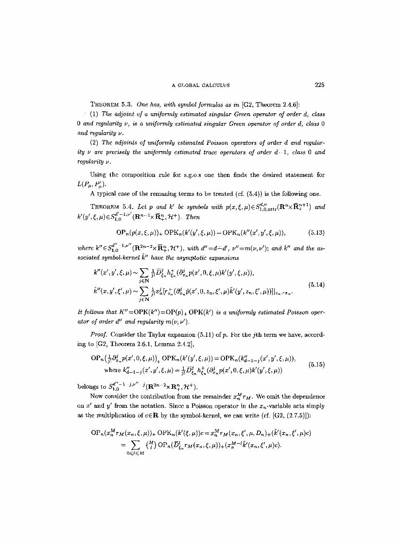
A G L O B A L C A L C U L U S 225
THEOREM 5.3. One has, with symbol formulas as in [G2, Theorem 2.4.6]:
(1) The adjoint of a uniformly estimated singular Green operator of order d, class 0 and regularity u, is a uniformly estimated singular Green operator of order d, class 0 and regularity u.
(2) The adjoints of uniformly estimated Poisson operators of order d and regular-
ity ~, are precisely the uniformly estimated trace operators of order d - l , class 0 and regularity u.
Using the composition rule for s.g.o.s one then finds the desired statement for
L(P~,P;~).
A typical case of the remaning terms to be treated (cf. (5.4)) is the following one.
d,v n - - n + l THEOREM 5.4. Let p and k' be symbols with p(x,~,p)ESl,O,uttr(R • ) and " " d ' - l ' U ' ( R n - l x - - "]~+). Then k' (y', ~, #) �9 ~1,o R~_,
OP~(p(x, ~, #))+ oPgu(k ' (y ' ,~ ,#) )=OPK~(k"(x ' ,y ' ,~ ,#) ) , (5.13)
where k" ' -~d"- l '~"~R2n-2xR ~ 7-/+), with d" "--1,0 ~ +, =d+d', u"=m(u , #) ; and k" and the as- sociated symbol-kernel k" have the asymptotic expansions
k " ( x ' , y ' , ~ , # ) ~ 1Dj h + , ~ "x' O" "k" '
jeN (5.14) [~"(x, y', r It) ~ ~ 1 x j rr + (w ~(~, z '
j ~ N
It follows that K"=OPK(k")=OP(p)+ OPK(k') is a uniformly estimated Poisson oper- ator of order d" and regularity re(u, # ) .
Proof. Consider the Taylor expansion (5.11) ofp. For the j t h term we have, accord-
ing to [G2, Theorem 2.6.1, Lemma 2.4.2],
OPn (~.O~,,p(x', 0, ~, #))+ OPK~(k'(y' , ~, #)) = OPKn(k~_l_ j (x', y', ~, #)), (5.15)
" 1 ~ j h4- (~,~p(x' , O, ~, t~)]g'(y', ~, ~)) where kd_l_j(x ' ,y ' ,~ ,# ) . ~. ~ , ~
d It 1 " v H " belongs to S - -J ' -J/R2~-2xR.'~ ?-/+). 1,0 ~ 4 - '
Now consider the contribution from the remainder x nMrM. We omit the dependence
on x' and y' from the notation. Since a Poisson operator in the xn-variable acts simply
as the multiplication of c � 9 by the symbol-kernel, we can write (cf. [G2, (2.7.5)]):
OP~(xffrM(xn,r OPK~(k'(~,#)) c = xUrn M(' Xn,~*' , / ~ , Dn)+(k'(Xn,~' ,Iz) c)
= Z (M) Op,(D~rM(X,~,~,#))+(xM_,~,(X~,~,,#)c).

226 G. GRUBB AND N. J. KOKHOLM
Assume that M>~d, and let N(d, l) be the smallest integer ~max(d- l , 0}, then M-l>~ N(d, l) for all tel0, M], and hence e+xM-'kteH2N(d't)(R). Since D~rM is of order d - l and regularity v- l , it satisfies (cf. (2.1))
D m i~ ~m'Dm'z~l r Zx
for all m,m'EN. Then we have in view of (5.1), that OP=(D~nrM ) maps H2d-l'~'(R)
into L2(R) with norm O(~-1+1) . This gives:
lit+ - l + M - l ' , OPn(D~ rM)(e x n k )IIL2(R+) ~ (e~'-l§
�9 v--l d - l -N(d l) N(d l) - -M- l t =(~, + l ) l l f fn ,~) , (5,~,~) 'nr k(SP)IIL~(R) N(d,l)
~(Qt~--IW1)xd--l--N(d'l) Z xN(d' l)-J J M - l - , IID~,,.(z= k )IIL.,(R+) j=O
J <~ ( e v - l _4_ 1 ) ( ~ v ' - M + l + 1)xd"-M-1/2 ~ (et/ '--M .~_ 1 ) z d " - M - 1 / 2 .
�9 �9 ;~ m m ' a j Apphcatmn of D~,,y, x,~ D ~ D~, Dg gives expressions that can be treated in the same way,
showing that for M sufficiently large (depending on the indices), one gets the correct
estimate. The proof of (5.14) is completed by taking this together with the information
on the symbols in (5.15). The composition rule for the full operators now follows as in
[G2, Theorem 2.7.9]. []
This proof is a little simpler than those in [G2, Lemmas 2.7.1-2, Theorem 2.7.3],
because we can use the global properties of p. When Theorem 5.4 is used to treat the
term P~,+K'~ in Theorem 5.1, one first brings K~ on y'-form.
The other compositions in (5.4) are treated in a very similar way, and this ends the
proof of Theorem 5.1.
By restriction to a fixed value of p, we get the corresponding (simpler) rules for
compositions and adjoints of parameter-independent systems:
COROLLARY 5.5. For p-independent systems with x-uniformly estimated symbols, the statements of Theorems 5.1 and 5.3 are valid when p and the regularity numbers are disregarded.
The rules are easily carried over to the situation of operators between admissible
vector bundles over manifolds, by use of the coordinate systems and partition of unity
described in Lemma 1.5. In fact, when we write
, - , - = ( ) ' A,A~ = Z ~j~ A , ~J20j3 A , Oj4, where ~j 0j 0 0 o Qy = ~j I t , ( 5 . 1 6 )
Jl,j2,J354 ~<Jo 0 Qj

A GLOBAL CALCULUS 227
the study of each term carries over to a study of compositions of operators on (1, ..., m} •
R~, where Theorem 5.1 can be apphed. Likewise, taking adjoints can be localized in
this way. Thus we can conclude:
COROLLARY 5.6. Theorems 5.1 and 5.3 extend to operators on admissible mani-
folds.
The calculus is hereby ready for the consideration of paxameter-elliptic Green oper-
ators in global Lp spaces, the consequences for parabolic problems, and the applications
to Navier-Stokes problems, established in continuations of this article [G5, 6].
References
[B] BEALS, R., L P and HSlder estimates for pseudodifferential operators: sufficient condi- tions. Ann. Inst. Fourier, 24 (1979), 239-260.
[B-L] BERGI-I, J. 8z L()FSTROM, J., Interpolation Spaces. Springer-Verlag, Berlin-New York, 1976.
IBM1] BOUTET DE MONVEL, L., Comportement d'un opdrateur pseudo-diffdrentiel sur une va~idtd ~ bord, I-II. J. Analyse Math., 17 (1966), 241-304.
IBM2] - - Boundary problems for pseudo-differential operators. Acta Math., 126 (1971), 11-51. [D] DONOGHUE JR., W. F., Monotone Matrix Functions. Grundlehren, 207. Springer-Verlag,
Berlin-New York, 1970. [El ESKIN, G., Boundary Value Problems for Elliptic Pseudodifferential Equations. AMS,
Providence, R. I., 1981. IF1] FRANKE, J., Besov-Triebel-Lizorkin spaces and boundary value problems, in Seminar
Analysis, 198J//85, pp. 89-104. Karl Weierstrass Institut fiir Math., Berlin, DDR, 1985.
IF2] - - Elliptische Randwertprobleme in Besov-Triebel-Lizorkin-Rai~men. Dissertation, Frie- drich Schiller Universit~it, Jena, 1986.
[Gi] GILBERT, J. E., Interpolation between weighted L p spaces. Ark. Mat., 10 (1972), 235- 249.
[G1] GRUBB, G., Singular Green operators and their spectral asymptotics. Duke Math. J., 51 (1984), 477-528.
[G2] - - Functional Calculus of Pseudo-Di]]erential Boundary Problems. Progr. Math., 65. Birkh~iuser, Boston, 1986.
[G3] - - Pseudo-differential boundary problems in Lp spaces. Comm. Partial Dij~erential Equations, 15 (1990), 289-340.
[G4] - -Parabol ic pseudo-differential boundary problems and applications, in Microlocal Analysis and Applications (Proceedings CIME, Montecatini Terme, 1989), pp. 46- 117. Lecture Notes in Math., 1495; by J. M. Bony, G. Grubb, L. HSrmander, H. Komatsu and J. SjSstrand (L. Cattabriga and L. Rodino, eds.). Springer-Verlag, Heidelberg, 1991.
[G5] - - 1. Parameter-elliptic and parabolic pseudodifferential boundary problems in global Lp Sobolev spaces. To appear in Math. Z. 2. Nonhomogeneous time-dependent Navier- Stokes problems in Lp Sobolev spaces. To appear; a preliminary version is given in Preprint no. 20, Copenhagen Univ. Math. Dept. Preprint Series, 1991.
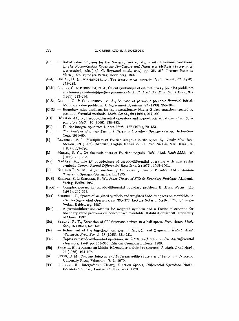
228 G. GRUBB AND N. J. KOKHOLM
[G6] - - Initial value problems for the Navier-Stokes equations with Neumann conditions, in The Navier-Stokes Equations II--Theory and Numerical Methods (Proceedings, Oberwolfach, 1991) (J. G. Heywood et al., eds.), pp. 262-283. Lecture Notes in Math., 1530. Springer-Verlag, Heidelberg, 1992.
[G-H] GRUBB, G. & HORMANDER, L., The transmission property. Math. Scand., 67 (1990), 273-289.
[G-K] GRUBB, G. ~/; KOKHOLM, N. J., Calcul symbolique et estimations Lp pour les probl~mes aux limites pseudo-diff~rentiels param~tris~s. C. R. Acad. Sci. Paris Sdr. I Math., 312 (1991), 223-226.
[G-S1] GRUBB, G. ~ SOLONNIKOV, V. A., Solution of parabolic pseudo-differential initial- boundary value problems. J. Differential Equations, 87 (1990), 256-304.
[G-S2] - - Boundary value problems for the nonstationary Navier-Stokes equations treated by pseudo-differential methods. Math. Scand., 69 (1991), 217-290.
[H1] H(3RMANDER, L., Pseudo-differential operators and hypoelliptic equations. Proc. Sym- pos. Pure Math., 10 (1966), 138-183.
[H2] - - Fourier integral operators I. Aeta Math., 127 (1971), 79-183. [H3] - - The Analysis of Linear Partial Differential Operators. Springer-Verlag, Berlin-New
York, 1983-85. ILl LIZORKIN, P. I., Multipliers of Fourier integrals in the space Lp. Trudy Mat. Inst.
Steklov., 89 (1967), 247-267; English translation in Proc. Steklov Inst. Math., 89 (1967), 269-290.
[M] MIHLIN, S. G., On the multipliers of Fourier integrals. Dokl. Akad. Nauk SSSR, 109 (1956), 701-703.
[Na] NAGASE, M., The L p boundedness of pseudo-differential operators with non-regular symbols. Comm. Partial Differential Equations, 2 (1977), 1045-1061.
[Ni] NIKOLSKI~, S. M., Approximation of Functions of Several Variables and Imbedding Theorems. Springer-Verlag, Berlin, 1975.
[R-S1] REMPEL, S. ~ SCHULZE, B.-W., Index Theory of Elliptic Boundary Problems. Akademie Verlag, Berlin, 1982.
[R-S2] - - Complex powers for pseudo-differential boundary problems II. Math. Nachr., 116 (1984), 269-314.
[Scl] SCItROHE, E., Spaces of weighted symbols and weighted Sobolev spaces on manifolds, in Pseudo-Differential Operators, pp. 360-377. Lecture Notes in Math., 1256. Springer- Verlag, Heidelberg, 1987.
[Sc2] - - A pseudodifferential calculus for weighted symbols and a Fredholm criterion for boundary value problems on noncompact manifolds. Habilitationsschrift, University of Mainz, 1992.
[Sel] SEELEY, R. T., Extension of C ~ functions defined in a half space. Proc. Amer. Math. Soc., 15 (1964), 625-626.
[Se2] - - Refinement of the functional calculus of CalderSn and Zygmund. Nederl. Akad. Wetenseh. Proc. Set. A, 68 (1965), 521-531.
[Se3] - - Topics in pseudo-differential operators, in CIME Con]erence on Pseudo-Differential Operators, 1968, pp. 169-305. Edizioni Cremonese, Roma, 1969.
[Sh] SHAMIR, E., A remark on Mihlin-HSrmander multipliers theorem. J. Math. Anal. Appl., 16 (1966), 104-107.
[St] STEIN, E. M., Singular Integrals and Differentiability Properties of Functions. Princeton University Press, Princeton, N. J., 1970.
IT1] TRIEBEL, H., Interpolation Theory, Function Spaces, Differential Operators. North- Holland Publ. Co., Amsterdam-New York, 1978.

A GLOBAL CALCULUS 229
IT2] IV-El
[Y]
- - Theory of Function Spaces. Birkh/iuser, Basel, 1983. VISI-IIK, M. I. gz I~SKIN, G. I., Elliptic equations in convolution in a bounded domain
and their applications. Uspekhi Mat. Nauk, 22 (1967), 15-76; English translation in Russian Math. Surveys, 22 (1967), 13-75.
M. YAMAZAKI, The LP-boundedness of pseudodifferential operators with estimates of parabolic type and product type. J. Math. Soc. Japan, 38 (1986), 199-225.
GERD GRUBB Department of Mathematics University of Copenhagen Universitetsparken 5 DK-2100 Copenhagen Denmark E-mail address: grubb~math.ku.dk
NIELS JORGEN KOKHOLM Department of Mathematics University of Copenhagen Universitetsparken 5 DK-2100 Copenhagen Denmark
Received October 15, 1991