low-order modeling from relay feedback

PROCESS DESIGN AND CONTROL

Low-Order Modeling from Relay Feedback

Qing-Guo Wang,* Chang-Chieh Hang, and Biao Zou

Department of Electrical Engineering, National University of Singapore, 10 Kent Ridge Crescent,Singapore 119260, Singapore

There have recently been considerable interests in extensions of PID relay autotuning to model-based controllers, and this necessitates transfer function modeling from relay feedback. Themethods reported in the literature for this purpose require two tuning tests, and their resultsare approximate in nature. In this paper, exact expressions for the periods and amplitudes oflimit cycles under relay feedback are derived for processes which may be modeled by first-orderplus dead-time dynamics. This time-domain information is then combined with frequencyresponse point estimation using Fourier series expansions of the limit cycles so that a first-order plus dead-time model can be identified with a single relay test. Furthermore, noapproximation is made in our derivations and the resultant model will be precise if it matchesthe structure of the process. In the case of the mismatched structure, it is shown throughextensive simulations that our procedure yields very accurate results in the sense that theidentified model frequency response fits the actual process one well. Both unbiased and biasedrelays with or without hysteresis are considered.

1. Introduction

Relay autotuning of PID controllers has been suc-cessful in industrial process control application and ledto a number of commercial autotuners (Astrom andHagglund, 1988). Now the relay feedback is beingextended to tune some other controllers, such as model-based controllers which need transfer function models(Hang et al., 1995; Palmor et al., 1994; Wang et al.,1995). The transfer function models (or their equivalentstep response models) also play an important role in theanalysis of the multivariable process. Luyben (1987)proposes the following method for first-, second-, andthird-order process modeling (called the ATV method):(1) The ultimate gain and ultimate frequency areobtained by using Astrom’s autotuning method. (2) Thedead time is read off from the initial response of thesystem to the autotuning test. (3) The steady-state gainis obtained from a steady-state model of the process orfrom use of the step response method (Luyben, 1990);(4) First-, second-, and third-order transfer functions arefitted to the data at zero and the ultimate frequencies.The procedure was later modified (Li et al., 1991) toremove the condition that the gain should be known.The modified procedure uses two relay experiments. Thefirst is a straightforward one; the second is run with adead time added. Thus, the steady-state gain can bedetermined. However, accurate measurement of thedead time from the initial response is very difficult, andthe ultimate gain and ultimate frequency derived fromthe describing function are approximate and may havesignificant errors in the case of processes with high-order dynamics and/or long dead times. Recently, aninput-biased relay experiment is introduced (Shen et al.,1996) to identify two points on the Nyquist curve froma single test based on the describing function analysis.

The most commonly used dynamic model for theindustrial process is the first-order plus dead-timemodel, which has three parameters. In this paper, exactexpressions for the periods and amplitudes of limitcycles under relay feedback are derived for first-orderplus dead-time processes. This time-domain informa-tion is combined with frequency response point estima-tion using Fourier series expansions of the limit cyclesso that a first-order plus dead-time model can beidentified with a single relay test. Our methods avoidthe difficulty of measuring the dead time from the relaytest. Furthermore, no approximation is made in ourderivations, and the resultant model will be precise ifit matches the structure of the process. In the case ofthe mismatched structure, it is shown through extensivesimulations that our procedure is robust and yields veryaccurate results in the sense that the identified modelfrequency response fits the actual process one well. Bothunbiased and biased relays with or without hysteresisare considered.The paper is organized as follows. In section 2,

modeling from a biased relay feedback is developed. Insection 3, the unbiased relay feedback is considered. Theconclusions are in section 4.

2. Biased Relay

Consider a first-order plus dead-time process

A relay feedback system of Figure 1 is set up for theprocess. In the ATV method (Luyben, 1987), only theapproximate critical point information of the processfrequency response can be obtained from one relay test.In order to obtain the steady-state gain of the processfrom the same relay experiment, in addition to thecritical point information, the biased relay as shown inthe Figure 2 is introduced. The resulting oscillation

* Author to whom all correspondence should be addressed.Tel: 65-7722282. Fax: 65-7791103. E-mail: [email protected].

G(s) ) Ke-Ls

Ts + 1(1)

375Ind. Eng. Chem. Res. 1997, 36, 375-381

S0888-5885(96)00412-5 CCC: $14.00 © 1997 American Chemical Society

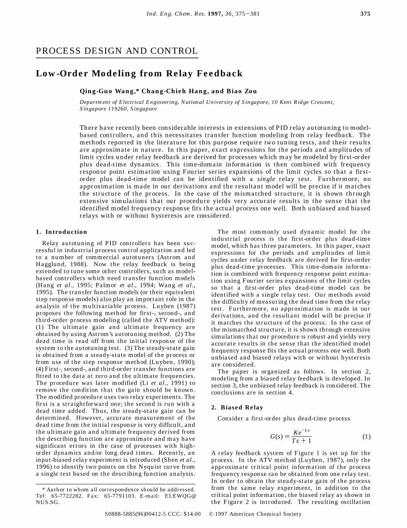
waveform of the process is shown in Figure 3. Thefollowing theorem gives the properties of the oscillation.Theorem 1: For the process of eq 1 under the relay

feedback of Figure 2, the process output y converges tothe stationery oscillation in one period (Tu1 + Tu2), andthe oscillation is characterized by

and

Proof: See the Appendix.Equations 2-5 are the exact expressions of the period

and the amplitude of limit cycle oscillation for theprocess (1). Some simulation examples are given inTable 1, where the outputs of biased relay are 1.3 and-0.7, respectively, and the hysteresis of relay is 0.1. Theresults show the accuracy of the formulas (2)-(5), andvery small errors are caused by simulation computa-tions.The four equations (2)-(5) are sufficient to determine

the three parameters of the process, but solving theseequations is somehow tedious. To simplify the compu-tations, we now look into frequency response informa-tion contained in the limit cycle. Theorem 1 indicatesthat the waveforms of the process input u(t) and outputy(t) are periodic with the period Tu1 + Tu2. They can beexpanded into Fourier series. The direct-current com-ponents of these periodic waves are extracted, and thesteady-state gain of the process can be computed(Ramirez, 1985) via the following formula:

With K known, the normalized dead time of theprocess Θ ) L/T is obtained from eq 2 or eq 3 as

or

It then follows from eq 4 or eq 5 that

or

The dead time is thus

The above development can be summarized as thefollowing identification procedure.Identification Procedure. The biased relay experi-

ment is performed. The process input u(t) and outputy(t) are recorded, and the periods and the amplitudesof the oscillation are measured.

Figure 1. Relay feedback system.

Figure 2. Biased relay.

Figure 3. Oscillatory waveforms under a biased relay feedback.

Table 1. Limit Cycle under the Biased Relay Feedback

process calculated result measured result percentage error, %

K T L Tu1 Tu2 Au Ad Tu1 Tu2 Au Ad Tu1 Tu2 Au Ad

1 2 1 1.620 2.503 0.5722 -0.3361 1.620 2.505 0.572 -0.336 0.000 0.080 0.035 0.0301 2 2 2.788 3.909 0.8585 -0.4793 2.790 3.910 0.859 -0.479 0.072 0.026 0.058 0.0631 2 5 5.972 7.307 1.2015 -0.6507 5.970 7.310 1.202 -0.651 0.034 0.041 0.042 0.0461 1 2 2.469 3.119 1.1376 -0.6188 2.470 3.120 1.138 -0.619 0.041 0.032 0.035 0.0321 5 2 3.432 5.447 0.4956 -0.2978 3.430 5.445 0.496 -0.298 0.058 0.037 0.081 0.0670.5 2. 2 3.003 4.321 0.4477 -0.2580 3.005 4.320 0.448 -0.258 0.067 0.023 0.067 0.0002 2 2 2.685 3.725 1.6803 -0.9218 2.685 3.725 1.680 -0.922 0.000 0.000 0.018 0.022

Au ) (µ0 + µ)K(1 - e-L/T) + εe-L/T (2)

Ad ) (µ0 - µ)K(1 - e-L/T) - εe-L/T (3)

Tu1 ) T ln2µKeL/T + µ0K - µK + ε

µK + µ0K - ε(4)

Tu2 ) T ln2µKeL/T - µK - µ0K + ε

µK - µ0K - ε(5)

K ) G(0) )∫0Tu1+Tu2y(t) dt∫0Tu1+Tu2u(t) dt

(6)

Θ ) ln(µ0 + µ)K - ε

(µ0 + µ)K - Au(7)

Θ ) ln(µ - µ0)K - ε

(µ - µ0)K + Ad(8)

T ) Tu1(ln 2µKeΘ + µ0K - µK + ε

µK + µ0K - ε )-1

(9)

T ) Tu1(ln 2µKeΘ - µ0K - µK + ε

µK - µ0K - ε )-1

(10)

L ) TΘ (11)

376 Ind. Eng. Chem. Res., Vol. 36, No. 2, 1997

Step 1: Compute K from eq 6.Step 2: Compute Θ from eq 7 or eq 8.Step 3: Compute T from eq 9 or eq 10.Step 4: Compute L from eq 11.Simulation is carried out for processes with different

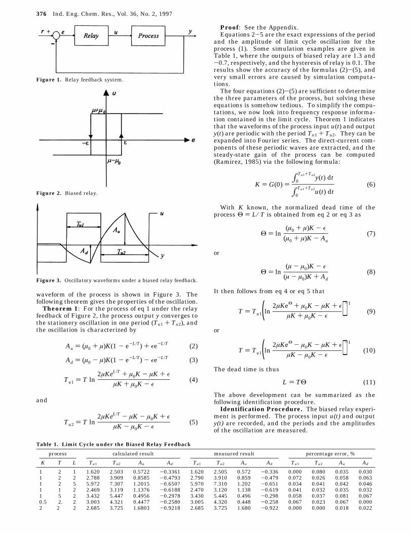
normalized dead time to illustrate the accuracy of theproposed method. The outputs of biased relay are 1.3and -0.7, respectively, and the hysteresis of relay is 0.1.The resultant limit cycles and model parameters arepresented in Table 2. For comparison, the parametersobtained by the ATV (Luyben, 1987) are also given inTable 2, where it is assumed that the steady-state gainis known and the dead time is read exactly. TheNyquist curves of the models and the corresponding realprocesses are shown in Figure 4. The results show thatthe proposed method can give nearly the exact identi-fication of the process parameters.

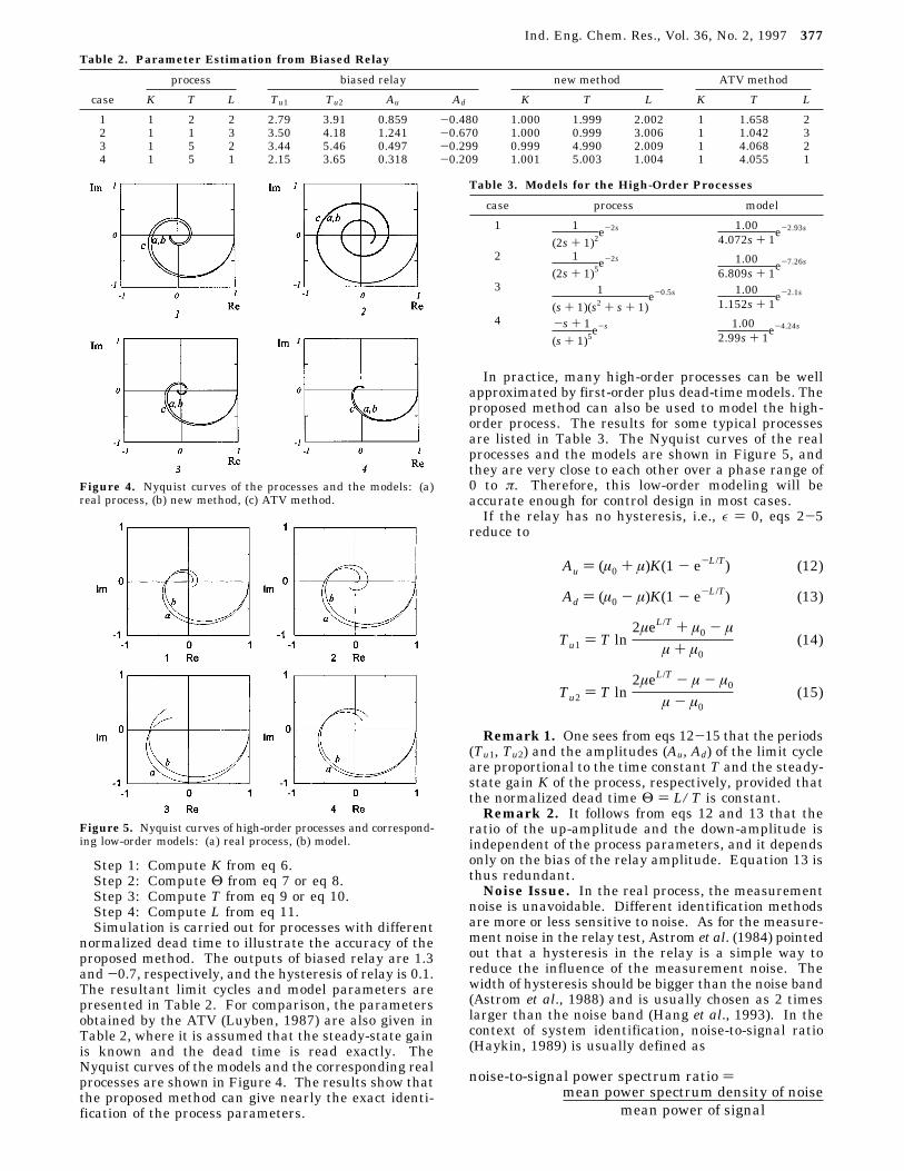
In practice, many high-order processes can be wellapproximated by first-order plus dead-time models. Theproposed method can also be used to model the high-order process. The results for some typical processesare listed in Table 3. The Nyquist curves of the realprocesses and the models are shown in Figure 5, andthey are very close to each other over a phase range of0 to π. Therefore, this low-order modeling will beaccurate enough for control design in most cases.If the relay has no hysteresis, i.e., ε ) 0, eqs 2-5

reduce to

Remark 1. One sees from eqs 12-15 that the periods(Tu1, Tu2) and the amplitudes (Au, Ad) of the limit cycleare proportional to the time constant T and the steady-state gain K of the process, respectively, provided thatthe normalized dead time Θ ) L/T is constant.Remark 2. It follows from eqs 12 and 13 that the

ratio of the up-amplitude and the down-amplitude isindependent of the process parameters, and it dependsonly on the bias of the relay amplitude. Equation 13 isthus redundant.Noise Issue. In the real process, the measurement

noise is unavoidable. Different identification methodsare more or less sensitive to noise. As for the measure-ment noise in the relay test, Astrom et al. (1984) pointedout that a hysteresis in the relay is a simple way toreduce the influence of the measurement noise. Thewidth of hysteresis should be bigger than the noise band(Astrom et al., 1988) and is usually chosen as 2 timeslarger than the noise band (Hang et al., 1993). In thecontext of system identification, noise-to-signal ratio(Haykin, 1989) is usually defined as

Table 2. Parameter Estimation from Biased Relay

process biased relay new method ATV method

case K T L Tu1 Tu2 Au Ad K T L K T L

1 1 2 2 2.79 3.91 0.859 -0.480 1.000 1.999 2.002 1 1.658 22 1 1 3 3.50 4.18 1.241 -0.670 1.000 0.999 3.006 1 1.042 33 1 5 2 3.44 5.46 0.497 -0.299 0.999 4.990 2.009 1 4.068 24 1 5 1 2.15 3.65 0.318 -0.209 1.001 5.003 1.004 1 4.055 1

Figure 4. Nyquist curves of the processes and the models: (a)real process, (b) new method, (c) ATV method.

Figure 5. Nyquist curves of high-order processes and correspond-ing low-order models: (a) real process, (b) model.

Table 3. Models for the High-Order Processes

case process model

1 1(2s + 1)2

e-2s 1.004.072s + 1

e-2.93s

2 1(2s + 1)5

e-2s 1.006.809s + 1

e-7.26s

3 1(s + 1)(s2 + s + 1)

e-0.5s 1.001.152s + 1

e-2.1s

4 -s + 1(s + 1)5

e-s 1.002.99s + 1

e-4.24s

Au ) (µ0 + µ)K(1 - e-L/T) (12)

Ad ) (µ0 - µ)K(1 - e-L/T) (13)

Tu1 ) T ln2µeL/T + µ0 - µ

µ + µ0(14)

Tu2 ) T ln2µeL/T - µ - µ0

µ - µ0(15)

noise-to-signal power spectrum ratio )mean power spectrum density of noise

mean power of signal

Ind. Eng. Chem. Res., Vol. 36, No. 2, 1997 377

(denoted by N1) or

(denoted by N2). In order to test our method in arealistic environment, real-time relay tests were per-formed using Dual Process Simulator KI 100 fromKentRidge Instruments (KentRidge, 1992). The simu-lator is an analog process simulator and can be config-ured to simulate a wide range of industrial processes

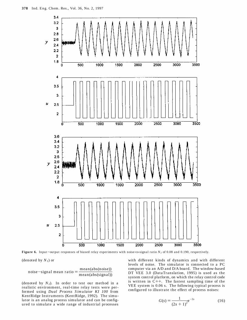
with different kinds of dynamics and with differentlevels of noise. The simulator is connected to a PCcomputer via an A/D and D/A board. The window-basedDT VEE 3.0 (DataTranslation, 1995) is used as thesystem control platform, on which the relay control codeis written in C++. The fastest sampling time of theVEE system is 0.06 s. The following typical process isconfigured to illustrate the effect of process noises:

Figure 6. Input-output responses of biased relay experiments with noise-to-signal ratio N2 of 0.08 and 0.190, respectively.

noise-signal mean ratio )mean(abs(noise))mean(abs(signal))

G(s) ) 1(2s + 1)2

e-2s (16)


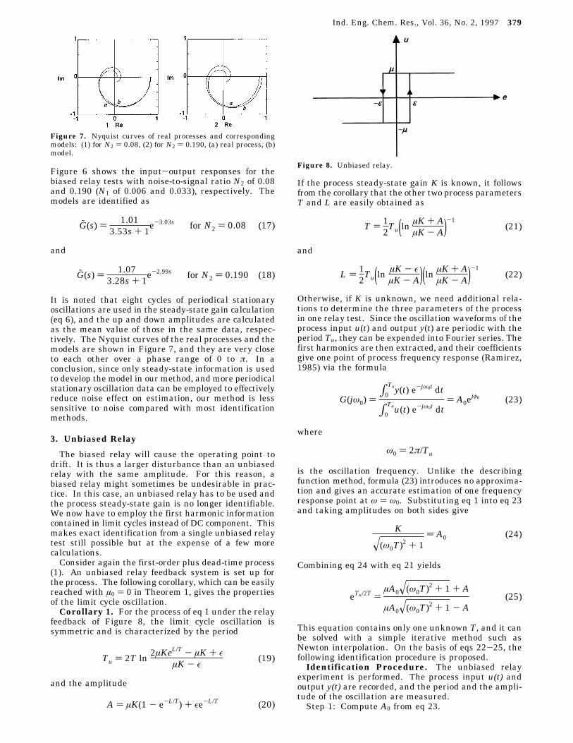
Figure 6 shows the input-output responses for thebiased relay tests with noise-to-signal ratio N2 of 0.08and 0.190 (N1 of 0.006 and 0.033), respectively. Themodels are identified as

and

It is noted that eight cycles of periodical stationaryoscillations are used in the steady-state gain calculation(eq 6), and the up and down amplitudes are calculatedas the mean value of those in the same data, respec-tively. The Nyquist curves of the real processes and themodels are shown in Figure 7, and they are very closeto each other over a phase range of 0 to π. In aconclusion, since only steady-state information is usedto develop the model in our method, and more periodicalstationary oscillation data can be employed to effectivelyreduce noise effect on estimation, our method is lesssensitive to noise compared with most identificationmethods.

3. Unbiased Relay

The biased relay will cause the operating point todrift. It is thus a larger disturbance than an unbiasedrelay with the same amplitude. For this reason, abiased relay might sometimes be undesirable in prac-tice. In this case, an unbiased relay has to be used andthe process steady-state gain is no longer identifiable.We now have to employ the first harmonic informationcontained in limit cycles instead of DC component. Thismakes exact identification from a single unbiased relaytest still possible but at the expense of a few morecalculations.Consider again the first-order plus dead-time process

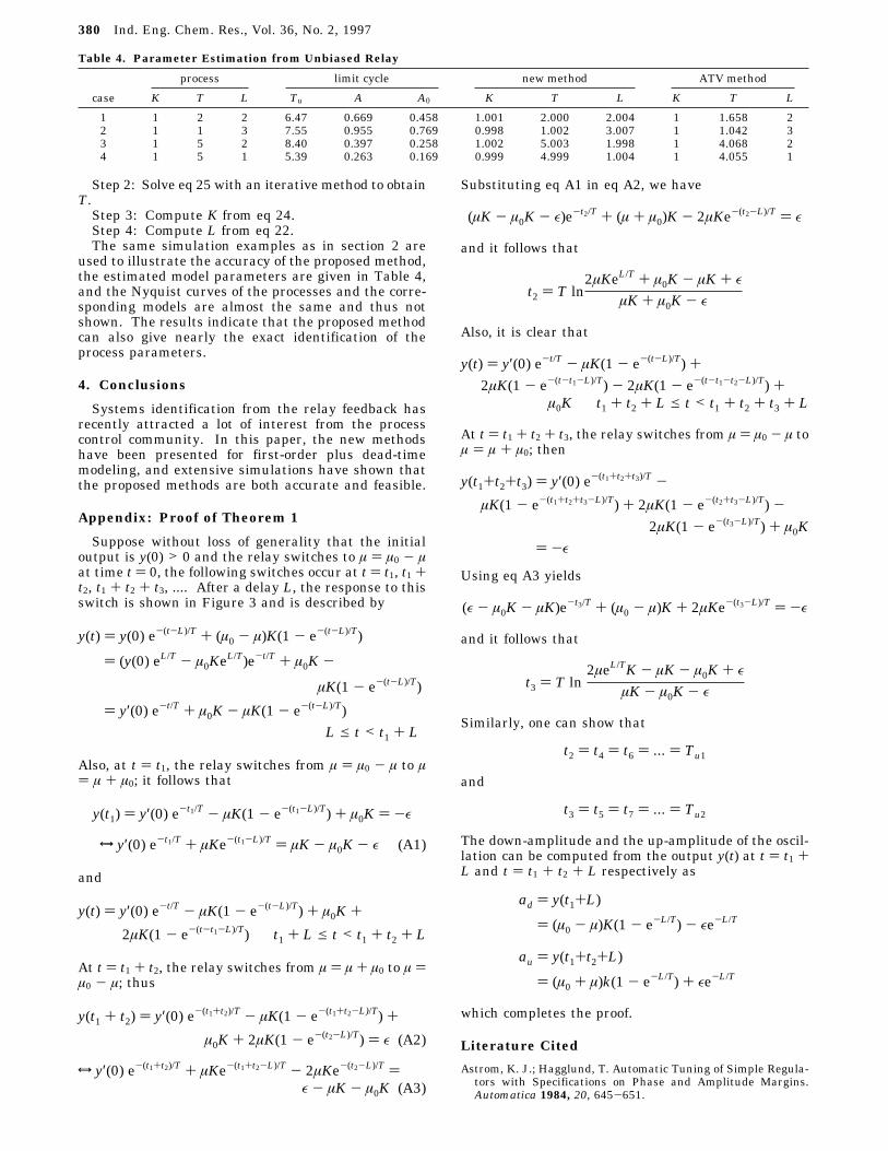
(1). An unbiased relay feedback system is set up forthe process. The following corollary, which can be easilyreached with µ0 ) 0 in Theorem 1, gives the propertiesof the limit cycle oscillation.Corollary 1. For the process of eq 1 under the relay

feedback of Figure 8, the limit cycle oscillation issymmetric and is characterized by the period

and the amplitude

If the process steady-state gain K is known, it followsfrom the corollary that the other two process parametersT and L are easily obtained as

and

Otherwise, if K is unknown, we need additional rela-tions to determine the three parameters of the processin one relay test. Since the oscillation waveforms of theprocess input u(t) and output y(t) are periodic with theperiod Tu, they can be expended into Fourier series. Thefirst harmonics are then extracted, and their coefficientsgive one point of process frequency response (Ramirez,1985) via the formula

where

is the oscillation frequency. Unlike the describingfunction method, formula (23) introduces no approxima-tion and gives an accurate estimation of one frequencyresponse point at ω ) ω0. Substituting eq 1 into eq 23and taking amplitudes on both sides give

Combining eq 24 with eq 21 yields

This equation contains only one unknown T, and it canbe solved with a simple iterative method such asNewton interpolation. On the basis of eqs 22-25, thefollowing identification procedure is proposed.Identification Procedure. The unbiased relay

experiment is performed. The process input u(t) andoutput y(t) are recorded, and the period and the ampli-tude of the oscillation are measured.Step 1: Compute A0 from eq 23.

Figure 7. Nyquist curves of real processes and correspondingmodels: (1) for N2 ) 0.08, (2) for N2 ) 0.190, (a) real process, (b)model.

G̃(s) ) 1.013.53s + 1

e-3.03s for N2 ) 0.08 (17)

G̃(s) ) 1.073.28s + 1

e-2.99s for N2 ) 0.190 (18)

Tu ) 2T ln 2µKeL/T - µK + ε

µK - ε(19)

A ) µK(1 - e-L/T) + εe-L/T (20)

Figure 8. Unbiased relay.

T ) 12Tu(ln µK + A

µK - A)-1

(21)

L ) 12Tu(ln µK - ε

µK - A)(ln µK + AµK - A)

-1(22)

G(jω0) )∫0Tuy(t) e-jω0t dt

∫0Tuu(t) e-jω0t dt) A0e

jφ0 (23)

ω0 ) 2π/Tu

K

x(ω0T)2 + 1

) A0 (24)

eTu/2T )µA0x(ω0T)

2 + 1 + A

µA0x(ω0T)2 + 1 - A

(25)


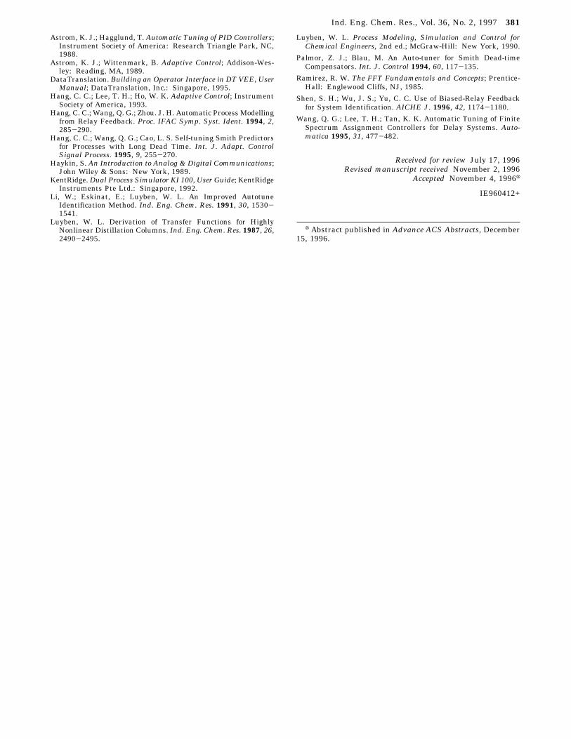
Step 2: Solve eq 25 with an iterative method to obtainT.Step 3: Compute K from eq 24.Step 4: Compute L from eq 22.The same simulation examples as in section 2 are

used to illustrate the accuracy of the proposed method,the estimated model parameters are given in Table 4,and the Nyquist curves of the processes and the corre-sponding models are almost the same and thus notshown. The results indicate that the proposed methodcan also give nearly the exact identification of theprocess parameters.

4. Conclusions

Systems identification from the relay feedback hasrecently attracted a lot of interest from the processcontrol community. In this paper, the new methodshave been presented for first-order plus dead-timemodeling, and extensive simulations have shown thatthe proposed methods are both accurate and feasible.

Appendix: Proof of Theorem 1

Suppose without loss of generality that the initialoutput is y(0) > 0 and the relay switches to µ ) µ0 - µat time t ) 0, the following switches occur at t ) t1, t1 +t2, t1 + t2 + t3, .... After a delay L, the response to thisswitch is shown in Figure 3 and is described by

Also, at t ) t1, the relay switches from µ ) µ0 - µ to µ) µ + µ0; it follows that

and

At t ) t1 + t2, the relay switches from µ ) µ + µ0 to µ )µ0 - µ; thus

Substituting eq A1 in eq A2, we have

and it follows that

Also, it is clear that

At t ) t1 + t2 + t3, the relay switches from µ ) µ0 - µ toµ ) µ + µ0; then

Using eq A3 yields

and it follows that

Similarly, one can show that

and

The down-amplitude and the up-amplitude of the oscil-lation can be computed from the output y(t) at t ) t1 +L and t ) t1 + t2 + L respectively as

which completes the proof.

Literature Cited

Astrom, K. J.; Hagglund, T. Automatic Tuning of Simple Regula-tors with Specifications on Phase and Amplitude Margins.Automatica 1984, 20, 645-651.

Table 4. Parameter Estimation from Unbiased Relay

process limit cycle new method ATV method

case K T L Tu A A0 K T L K T L

1 1 2 2 6.47 0.669 0.458 1.001 2.000 2.004 1 1.658 22 1 1 3 7.55 0.955 0.769 0.998 1.002 3.007 1 1.042 33 1 5 2 8.40 0.397 0.258 1.002 5.003 1.998 1 4.068 24 1 5 1 5.39 0.263 0.169 0.999 4.999 1.004 1 4.055 1

y(t) ) y(0) e-(t-L)/T + (µ0 - µ)K(1 - e-(t-L)/T)

) (y(0) eL/T - µ0KeL/T)e-t/T + µ0K -

µK(1 - e-(t-L)/T)

) y′(0) e-t/T + µ0K - µK(1 - e-(t-L)/T)L e t < t1 + L

y(t1) ) y′(0) e-t1/T - µK(1 - e-(t1-L)/T) + µ0K ) -ε

S y′(0) e-t1/T + µKe-(t1-L)/T ) µK - µ0K - ε (A1)

y(t) ) y′(0) e-t/T - µK(1 - e-(t-L)/T) + µ0K +

2µK(1 - e-(t-t1-L)/T) t1 + L e t < t1 + t2 + L

y(t1 + t2) ) y′(0) e-(t1+t2)/T - µK(1 - e-(t1+t2-L)/T) +

µ0K + 2µK(1 - e-(t2-L)/T) ) ε (A2)

S y′(0) e-(t1+t2)/T + µKe-(t1+t2-L)/T - 2µKe-(t2-L)/T )ε - µK - µ0K (A3)

(µK - µ0K - ε)e-t2/T + (µ + µ0)K - 2µKe-(t2-L)/T ) ε

t2 ) T ln2µKeL/T + µ0K - µK + ε

µK + µ0K - ε

y(t) ) y′(0) e-t/T - µK(1 - e-(t-L)/T) +2µK(1 - e-(t-t1-L)/T) - 2µK(1 - e-(t-t1-t2-L)/T) +

µ0K t1 + t2 + L e t < t1 + t2 + t3 + L

y(t1+t2+t3) ) y′(0) e-(t1+t2+t3)/T -

µK(1 - e-(t1+t2+t3-L)/T) + 2µK(1 - e-(t2+t3-L)/T) -2µK(1 - e-(t3-L)/T) + µ0K

) -ε

(ε - µ0K - µK)e-t3/T + (µ0 - µ)K + 2µKe-(t3-L)/T ) -ε

t3 ) T ln2µeL/TK - µK - µ0K + ε

µK - µ0K - ε

t2 ) t4 ) t6 ) ... ) Tu1

t3 ) t5 ) t7 ) ... ) Tu2

ad ) y(t1+L)

) (µ0 - µ)K(1 - e-L/T) - εe-L/T

au ) y(t1+t2+L)

) (µ0 + µ)k(1 - e-L/T) + εe-L/T


Astrom, K. J.; Hagglund, T. Automatic Tuning of PID Controllers;Instrument Society of America: Research Triangle Park, NC,1988.

Astrom, K. J.; Wittenmark, B. Adaptive Control; Addison-Wes-ley: Reading, MA, 1989.

DataTranslation. Building an Operator Interface in DT VEE, UserManual; DataTranslation, Inc.: Singapore, 1995.

Hang, C. C.; Lee, T. H.; Ho, W. K. Adaptive Control; InstrumentSociety of America, 1993.

Hang, C. C.; Wang, Q. G.; Zhou. J. H. Automatic Process Modellingfrom Relay Feedback. Proc. IFAC Symp. Syst. Ident. 1994, 2,285-290.

Hang, C. C.; Wang, Q. G.; Cao, L. S. Self-tuning Smith Predictorsfor Processes with Long Dead Time. Int. J. Adapt. ControlSignal Process. 1995, 9, 255-270.

Haykin, S. An Introduction to Analog & Digital Communications;John Wiley & Sons: New York, 1989.

KentRidge.Dual Process Simulator KI 100, User Guide; KentRidgeInstruments Pte Ltd.: Singapore, 1992.

Li, W.; Eskinat, E.; Luyben, W. L. An Improved AutotuneIdentification Method. Ind. Eng. Chem. Res. 1991, 30, 1530-1541.

Luyben, W. L. Derivation of Transfer Functions for HighlyNonlinear Distillation Columns. Ind. Eng. Chem. Res. 1987, 26,2490-2495.

Luyben, W. L. Process Modeling, Simulation and Control forChemical Engineers, 2nd ed.; McGraw-Hill: New York, 1990.

Palmor, Z. J.; Blau, M. An Auto-tuner for Smith Dead-timeCompensators. Int. J. Control 1994, 60, 117-135.

Ramirez, R. W. The FFT Fundamentals and Concepts; Prentice-Hall: Englewood Cliffs, NJ, 1985.

Shen, S. H.; Wu, J. S.; Yu, C. C. Use of Biased-Relay Feedbackfor System Identification. AICHE J. 1996, 42, 1174-1180.

Wang, Q. G.; Lee, T. H.; Tan, K. K. Automatic Tuning of FiniteSpectrum Assignment Controllers for Delay Systems. Auto-matica 1995, 31, 477-482.

Received for review July 17, 1996Revised manuscript received November 2, 1996

Accepted November 4, 1996X

IE960412+

X Abstract published in Advance ACS Abstracts, December15, 1996.


low-order modeling from relay feedback

Documents