low coherence interferometry in turbomachinery and flow
TRANSCRIPT

Research Collection
Doctoral Thesis
Low coherence interferometry in turbomachinery and flowvelocimetry
Author(s): Kempe, Andreas
Publication Date: 2007
Permanent Link: https://doi.org/10.3929/ethz-a-005344464
Rights / License: In Copyright - Non-Commercial Use Permitted
This page was generated automatically upon download from the ETH Zurich Research Collection. For moreinformation please consult the Terms of use.
ETH Library

Diss. ETH No. 16962
Low Coherence Interferometry In
Turbomachinery and Flow Velocimetry
A dissertation submitted to the
Swiss Federal Institute of Technology Zurich
for the degree of
Doctor of Science
presented by
Andreas Kempe
Dipl.-Ing. TU Dresden
born September, 7, 1977
citizen of Germany
accepted on the recommendation of
Prof. Dr.-Ing. Thomas Rosgen, supervisor
Ken Yves Haffner, co-examiner
2007

Copyright (c) 2007 Andreas KempeInstitute of Fluiddynamies (ETH Zurich)
All rights reserved
Low Coherence Interferometry In
Turbomachinery and Flow Velocimetry
Published and distributed by
Institute of Fluiddynamies
Swiss Federal Institute of Technology (ETH) Zurich
ETH Zentrum, ML H35
CH-8092 Zurich
Switzerland
http //www lfd mavt ethz ch
Printed in Switzerland by
Repro ETH Honggerberg
Wolfgang-Pauh-Str 15, HIL C 45
CH-8093 Zurich
Switzerland
Acknowledgments
The work on this thesis was always inspiring and exciting, sometimes it was chal¬
lenging and also attntional, but overall it was a very interesting and unforgettable
experience. Its success has been made possible by the help of many other people.
Thus, I want to express my gratitude to everybody for supporting me in my research.
In particular I would like to thank my supervisor Prof. Dr.-Ing. Thomas Rosgen,who has given me the chance to participate in interesting research projects and at¬
tend various international conferences. He also gave me the opportunity for a research
visit at the California Institute of Technology, which was a very unique experience
for me. During the daily work he has supported me with his encouragement and he
has always shown his interest in my research - leading to many discussions.
I want also thank my co-supervisor Ken Y. Haffner for his fruitful recommenda¬
tions to write this thesis as a summary of my research work. Particularly, I would like
to express my sincere thanks to him again as my research partner within ALSTOM
Power. Without his help the success of the project would not has been possible.With his unresting engagement he paved the way for tests at a full sized gas turbine.
The test series at such a "hell of a machine" was a really exciting experience for
me. Concerning the work together with ALSTOM Power, I have to thank for the
financial support to the project, too.
A special thanks also goes to Dr. Stefan Schlamp who greatly enriched my knowl¬
edge with his exceptional insights into the academical research. The close coopera¬
tion with him in writing papers helped me overcomethis - disliked by me - aspect of
the academic work. I also have to thank him for always listening to all of my new
ideas, it was the fastest way to smash them down or to decide to give it a try.
Last but not least, sincere thanks go to my lovely ones my parents and of course
my girlfriend. For my parents I don 't have to enumerate what they have done for me.
I just want to say Danke! Et pour ma petite amie je la remercie pas uniquement
grâce à son ordinateur que j'ai pu utiliser pour écrire ma thèse mais pour beaucoup
plus! Un gros bisou!


Contents
Acknowledgments iii
List of Figures / Tables ix
Notations xi
Zusammenfassung / Abstract xiii
I. Theory 3
Introduction 3
1 Fundamentals of Lasers and Optics 5
1.1 Electromagnetic Waves 5
1.1.1 Mathematical Description 5
Homogeneous Plane Waves 6
1.1.2 Light Polarization 7
1.1.3 Mixing of Electromagnetic Waves 7
1.1.4 Laser Light 8
Monochromatic Light 8
Non-Monochromatic Light 8
Optical Coherence Temporal/Spatial 9
1.2 Optical Components 11
1.2.1 Photodetectors 11
Technical Characteristics 12
1.2.2 Optical Fibers 14
Multimode Step-Index Fiber 14
Multimode Graded-Index Fiber 15
Singlemode Fiber 15
1.2.3 Optical Gratings and Bragg Cells 16
Diffraction Grating 16
Bragg Cells 17
1.2.4 Superluminescent Light Emitting Diodes (SLD's) 17
v

2 Interferometry 19
2.1 Michelson-Interferometer 19
2.2 Low Coherence Interferometry (LCI) 20
2.2.1 Principle 21
2.2.2 Low Coherence Interferometry Applications 23
Optical Coherence Tomography - OCT 23
Optical Low Coherence Reflectometry - OLCR 24
Distributed Laser-Doppler Velocimetry - DLDV 24
3 Laser Velocimetry 25
3.1 Light Scattering of Small Particles 25
3.2 Laser-Doppler Systems 26
3.2.1 The Doppler Effect 26
3.2.2 Laser-Doppler Velocimetry - LDV 26
LDV - Doppler Difference Method 27
LDV - Reference Beam Method 27
3.3 Laser-2-Focus Systems (L2F) 29
3.3.1 Principle 29
3.3.2 Correlation Method 30
3.3.3 Histogram Method 31
II. Tip Clearance Probe 35
Introduction and Motivation 35
4 Turbomachinery Background 37
4.1 Tip Clearance/Leakage Flows 37
4.2 Clearance Effects in Turbines 38
4.2.1 Losses 38
4.2.2 Heat Transfer 40
5 Experimental Setup 41
5.1 Measurement Principle/Optical Arrangement 41
5.2 Optical Frontend 42
5.3 Signal Processing 43
5.3.1 Data Acquisition 43
5.3.2 Data Analysis 44
6 Experiments 47
6.1 System Performance 47
6.2 LISA Turbine Tests 47
6.3 GT26 Gas Turbine Tests 50
7 Conclusions / Outlook 53

III. Self-Referencing Velocimetry 57
Introduction and Motivation 57
8 Self-Referencing Low Coherence Velocimeter 59
8.1 Basic Working Concept 59
8.2 Self-Referencing Laser-Doppler Velocimetry (SR-LDV) 59
8.2.1 Measurement Principle- SR-LDV 59
8.2.2 Data Analysis - SR-LDV 62
8.3 Self-Referencing Laser-Two-Focus Velocimetry (SR-L2F) 63
8.3.1 Measurement Principle- SR-L2F 63
8.3.2 Data Analysis - SR-L2F 64
9 Experiments 67
9.1 Signal Processing 67
9.2 Measurements in Liquid Flows 68
9.2.1 Poiseuille Flow- Rectangular Channel 68
9.2.2 Couette Flow - Rotating Cylinder 69
9.3 Gaseous Flows 73
9.3.1 Flow Seeding 73
9.3.2 Blasius Solution - Flat Plate 74
10 Measurement Uncertainty Considerations for SR-LDV 77
10.1 General Measurement Precision 77
10.2 Aperture Broadening 77
10.3 Shadowing Effect 78
10.4 Frequency Resolution 79
11 Conclusions / Outlook 81
11.1 Summary 81
11.2 Dual Beam Self-Referencing Laser Doppler Velocimeter 82
Appendix 89
Bibliography 89
Epilogue 93
Curriculum Vitae 95


List of Figures / Tables
Figures
1.1 Laser pulse, complex degree of coherence and power spectral density. 10
1.2 Responsivity of a photoreceiver - Newport model 1811 12
1.3 Types of optical fibers 15
1.4 Performance of SLD-HP-56-HP 18
2.1 Basic principle of a Michelson interferometer 20
2.2 Low coherence interferometry principle 21
2.3 Interferogram of Superlum SLD-HP-56-HP 23
3.1 Scattering behavior of small particles 25
3.2 Basic principle for LDA techniques (direct backward scattering). . . 26
3.3 LDA dual-beam configuration 28
3.4 Basic principle LDV - reference beam method 28
3.5 L2F orientation of the measurement volumes 29
3.6 L2F flow orientation a.) correlation possible b.) no correlation.... 29
3.7 3D distribution curve of a L2F measurements series 30
3.8 Statistical distribution of a L2F measurement at a fix angle 31
4.1 Secondary flow field of an axial-turbine stage 37
4.2 Sources of turbine losses 38
4.3 Loss vs. reduced blade area 39
4.4 Turbine efficiency vs. tip clearance 39
4.5 Sheerwood number representing amount of heat transfer 40
5.1 Schematic setup of the optical parts for the tip clearance probe. ...41
5.2 Interaction between laser beam, front end and blade tip 42
5.3 Photograph of the tip clearance probe SFE 43
5.4 Data acquisition - tip clearance probe 44
5.5 Sample intensity map for a turbine blade on a rotary stage, 40 /im
delay steps, 5 ßs sliding window 45
6.1 Schematic view of LISA axial test turbine 47
6.2 Tip clearance distribution of LISA rotor, intensity map 48
6.3 LISA tip clearance behavior over operation time 49
6.4 GT26 example intensity plot of several blade passages 50
6.5 GT26 schematic illustration 51
8.1 Schematic setup of the optical components in the interferometer unit,
which also includes the light source 60
IX

8.2 Self-referencing LDV - schematic setup of the interaction between
laser beams and particles 61
8.3 Self-referencing L2F principle 65
8.4 Particle passages bandpass filtered signal, raw signal 65
9.1 Data acquisition - boundary layer profiler 67
9.2 Optical access - rectangular channel experiment 68
9.3 Poiseuille flow profile measured with SR-LDV and SR-L2F 69
9.4 Measured velocity profile of Couette flow at 0.21 m/s surface speed. 70
9.5 Measured velocity profiles of Couette flow at various rotation speeds. 71
9.6 Standard deviation/errors - Couette flow experiment 72
9.7 Flat plate wind tunnel schematic 74
9.8 Optical access through clear adhesiv tape, sensor head positioning. . 75
9.9 Measured profiles - flat plate experiment 75
10.1 Aperture broadening (black), shadowing effect (gray) 79
11.1 Dual beam self-referencing LDV interferometer design 82
11.2 Dual beam self-referencing LDV principle 83
Tables
1.1 Spectral bandwidths and coherence lengths of various light sources. . 8
11.1 Combinations of the ray subpairs with equal pathlengths. 84

Notations
All bold letters represent vectors, underlines denote the complex from. The latin
letters x, y, z represent the cartesian coordinates, u,v,w the corresponding velocities
in [m/s].
Latin Letters
Symbol Unit Description
A m? area
si — autocorrelation function
B T magnetic induction
b m width
c,c0 m/s speed of light, ~ in vacuum
D C/m? electric displacementd m distance
E V/m electric field strengthS J/Hz energy spectral densitye — unit vector
& — Fourier transformation function
is? - factor for the shape of the power spectral density
JjJcjJshzft Hz frequency, cut-off~,
~ shift
G - photodetector gain factor
H A/m magnetic field strengthh eVs Planck constant
I W/m2 electromagnetic intensity
^di îjn > îp> A photodiode dark current, ~ Johnson-Nyquist noise
*SÄT)*sn current, ~ electric current, ~ reverse saturation
current, ~ shot noise current
k - wavenumber
kß eV/K Boltzmann constant
l,lc m length, coherence ~
m kg mass
mv - modulation depth / visibilityNA - numerical aperture
NEP W/VHz noise equivalent power
n,neff- refractive index, effective refractive index
P - Poynting vector
Pp w photodiode power
&>,!p W/Hz, - power spectral density, normalized ~
Q - bragg cell quality factor
Q C elemental chargeRe - Reynolds number
continued on next page
XI

Symbol Unit Description
R\ A/WRsh n
f-, fcore m
s A/m2s —
T K
Ta —
t,tf s
V -
VA V
V, Vr, Vp m/sVA V
w J/m?
spectral responsivity
photodiode shunt resistance
radius, ~ of fiber core
current density
signalabsolute temperature
Taylor number
time, ~ of flight
optical fiber V-parameter
applied bias voltage
velocity, relative~, particle r
applied bias voltage
energy density
Greek Letters
Symbol Unit Description
ß rod
7 -
A -
e, e0 F/m
V Pas
Vq-
e rod
K S/mA,A0 m
A m
ß,ßo N/A2Pc C/m3T,TC s
abroad-
<P rod
UJ Hz
angleself coherence function
difference
electric permittivity, ~ in vacuum
dynamic viscosity
quantum efficiency
angleelectric conductivity
light wavelength, ~ in vacuum
acoustic wavelength
magnetic permeability, ~ in vacuum
charge densitytime incremental, coherence time
broadening factor
phase angle27rf - angular frequency
Abbreviations
Symbol Description
AOM acousto-optic modulator
DSO digital storage oscilloscope
LCI low coherence interferometry
EFE, SFE endoscopic front end, sensor front end
SR self-referencing

Zusammenfassung
Diese Doktorarbeit enstand in den Jahren 2002 bis 2006 am Institut fur Fluiddyna-
mik, ETH Zurich. Die Arbeit wurde hauptsächlich durch ALSTOM Power Switzer¬
land im Rahmen der Kooperation Center of Energy Conversion - CEC finanziert.
Es werden zwei neue Messmethoden fur die Anwendung von Niedrig-KoharenzInterferometne vorgestellt. Zum einen konnte zum ersten Mal die Tip Clearance
(Schaufelabstand) der ersten Laufreihe nach der Brennkammer einer Kraftwerks¬
gasturbine unter realen Bedingungen akkurat gemessen werden. Zum anderen wurde
ein neues Laser-Anemometer entwickelt, welches auf einfache Weise erlaubt Grenz¬
schichten auf bewegten Oberflachen zu messen.
Die Entwicklung der Tip Clearance Messsonde war das ursprüngliche Projekt. Es
wurde ein System entwickelt mit dem zeitlich aufgloste Abstandsmessungen an der
ersten der Brennkammer folgenden Laufreihe einer Gasturbine durchgeführt werden
können. Das Prinzip basiert auf der Interferenz zwischen dem Streulicht einer vor-
beilaufenden Turbinenschaufel und dem einer Referenz im Turbinengehause. Zur
Zeit gebräuchliche Sensoren haben entweder eine zu geringe zeitliche Auflosung,einen zu geringen Messbereich oder sind bei sehr hohen Temperaturen (> 1000°C)nicht dauerhaft anwendbar. Niedrig-Koharenz Interferometne erlaubt eine hohe zeit¬
lich Auflosung (fij 1 ßs) mit einer absoluten Messgenauigkeit im Bereich von unter
einem hundertstel Millimeter. Der Sensorkopf kann daher in einer gekühlten Kavitat
platziert werden ohne an Messgenauigkeit einzubussen. Ein faseroptischer Prototypwurde erfolgreich auf einer Laborturbine mit Kaltgas, als auch in einer grossen Kraft-
werksgasturbine (GT26-ALSTOM) getestet. Der zweite Teil dieser Doktorarbeit be¬
schreibt die Funktionsweise dieses Sensors und gibt eine Zusammenfassung zu den
Testmessungen.
Ein neues selbst referenzierende Laser-Anemometer kombiniert Techniken der Ge¬
schwindigkeitsbestimmung mit den Eigenschaften der Niedrig-Koharenz Interfero¬
metne (hochaufgeloste Abstandsmessung). Als neuer Ansatz sind sowohl das Mess¬
objekt als auch die Referenz ausserhalb des Interferometers platziert und somit
einander selbst referenzierend. Dies erlaubt kontaktlose Messungen von wandnahen
Strömungen auch wenn sich die Oberflache unregelmassig bewegt. Durch die
Interferometereinstellung wird ohne den Sensorkopf zu bewegen die Messpositionautomatisch bezüglich der Oberflache fixiert. Die absolute Genauigkeit der räumlich
Auflosung hegt im Mikrometerbereich und wird durch die Eigenschaften der niedng-koharenten Lichtquelle definiert. Mit einer Weisshchtquelle waren daher theoretisch
auch räumliche Aufiosugen im sub-mikrometer Bereich möglich. Der dritte Teil dieser
Arbeit beschreibt das Prinzip der neuen Methode und stellt die Ergebnisse aus ersten
Validierungtests vor.


Abstract
The work reported in this thesis was carried out at the Institute of Fluid Dynamics,ETH Zurich, between 2002 and 2006. The work was mainly funded by ALSTOM
Power Switzerland as a part of the Center of Energy Conversion - CEC co-operation
between ETH and ALSTOM.
This thesis introduces two novel methods for sensing applications in low coherence
interferometry. For the first time under operating conditions the tip clearance of an
early stage of a power plant gas turbine has been measured in detail. On the other
hand a new technique of laser velocimetry has been developed, allowing contactless
boundary layer measurements over moving surfaces.
The "Tip Clearance Probe" was the initial project. This measuring system has
been developed to obtain temporally resolved tip clearance data from early stages of
gas turbines. The working principle relies on the interference between backreflected
light from the blade tips during the blade passage time and a frequency shifted
reference. Common tip clearance sensors either do not have the temporal resolution
or an adequate measurement range or they cannot withstand the high temperature
loads. The low coherence interferometry technique adapted to tip clearance sensing
allows to measure with absolute spatial accuracy of tens of microns. The probe can
hence be mounted in a cooled recess without compromising accuracy. A prototype
of the system, an all-fiber assembly, has been successfully applied to a laboratory
cold-gas turbine and to the first stage behind the combustor of a large-scale power
generation gas turbine (GT26-ALSTOM). The second part of this thesis outlines the
principle of this sensor and reports on the turbine measurements.
The novel "Self-Referencing Boundary Layer Profiler" combines flow velocimetrymeasurements with the spatial high resolving qualities of low coherence interfer¬
ometry. The new approach is that both the object to be measured and an opticalreference are outside of the interferometer, i.e., they are self-referenced to each other.
Thus, the technique is applicable to contactless measurements of near surface flows,even if the surface moves irregularly. The measurement location is always selected
based on its distance to an reference object. The distance can be adjusted without
moving optical parts in the sensor head, but by varying the path lengths in the
interferometer arms. The absolute accuracy of the measurement location and the
spatial resolution depend on the properties of the low coherence light source, with
typical values of tens of microns. The working principle of this new technique and
proof-of-pnnciple tests are described in the third part of this thesis.


Part I
Theory
i


Introduction
This part of the thesis is intended to give a brief overview about relevant fields
of optics, lasers, interferometry and laser velocimetry. Together with a number of
historical facts only basic background knowledge is presented, not claiming com¬
pleteness. For further information one can follow the given references used as source
of this short summary.
The term optics originates form the greek phrase téchnë optikë, respectively from
the latin phrase ars optica, both meaning the lore relevant for vision (Kahske, 1996).Thereby, this stands for the science of light, with its origination, propagation and
perception. In the sense of natural sciences this means the physics of electromagnetic
radiation, wherein the visible light is only a small part. Electromagnetic waves as
a major part of todays physics exhibit a variety of exciting phenomena, which are
often simply fascinating for everybody.
Historical deliverances about optics go back to first great civilizations, such as the
ancient Babylon or Egypt. So, empirical knowledge about light reflection and the
straight propagation of light was already existent. Nevertheless, light had almost
everywhere some form of spiritual character. Between 500 B.C. and 200 the Greeks
Empedokles, Plato, Euklid, Aristoteles, Archimedes, Claudius and Ptolemaus have
been involved in the development of knowledge about light in the scientific sense.
The Greek already could mathematically describe light reflection and refraction. It
was also known that human vision is only possible when something is illuminated
by light. Unfortunately, due to the fact that Aristoteles disliked experiments, the
Greek and also later theories were partly incorrect, simply because sometimes theywere not verified at all.
After the Hellenistic civilization many of their scientific writings has been de¬
stroyed in wars or they got lost. Around the year 1000, Alhazen Mohammed Ibn
el Heitam, a persian scientist, wrote an opus "Kitab-al-Manazir" (treasure of op¬
tics). His theories were based on the old Greek papers. In the Europe of the Mid¬
dle Age most scientists shared Aristoteles attitudes. First with Robert Grosseteste
(1168/75-1253) and mainly with his student Roger Bacon (1214-1294) experiment
and theory together were seen as the way of science. With the translation of the
theories of Ptolemaus and Ibn el Heitam into Latin by the end of the 12th century,the knowledge of optics in Europe slowly increased.
From then on many scientists and also painters became aware of novel optical laws
and they developed their own theories, e.g., Isaac Newton (1643-1727) and Leonardo
da Vinci (1452-1519). A real breakthrough was achieved in 1817 by Thomas Young,since he first saw light as a transversal wave. Independently, Augustin Fresnel devel¬
oped similar theories around the same time. In 1845 Micheal Faraday (1791-1867)found a first indication for a relationship between light and electromagnetism. He
3
showed experimentally that the polarization of light can be rotated by a magnetic
field. Following this suggestion, James Clerk Maxwell (1831-1879) developed the
theory of electromagnetic waves, which up to today is mainly used to describe the
behavior of light. Nevertheless, in 1900 Max Planck (1858-1947) opened the book
to the quantum mechanics and in turn also the development of lasers (light amplifi¬cation by stimulated emission) in the mid 1950's.
Today, scientists are still actively conducting research in the field of light, e.g.,
quantum optics and non-classical light. So, for thousands of years light has fascinated
many researchers and everybody else alike, and for sure it will continue to do so.
4

1 Fundamentals of Lasers and Optics
The description of electromagnetic waves presented in this thesis mainly follows
the book "Laser Doppler and Phase Doppler Measurement Techniques. "(Albrechtet al., 2003). For consistency the given equations for electromagnetic waves follow
their nomenclature. Only differing references are explicitly cited.
1.1 Electromagnetic Waves
1.1.1 Mathematical Description
Light propagation can be described by the theory of electromagnetic fields, which is
based on Maxwell's equations. For a harmonic oscillation, Maxwell's equations can
be simplified by using the complex form (denoted through underlines)
curlH = S + jwD_, curlE=-jwB_ (11a)
divD = ,3c, divB = 0 (lib)
S = eE, D = kE, B = /uH (lie)
with H as the magnetic field strength, S as the current density, u> as the angular
frequency, D as the electric displacement, E as electric field strength, B as the
magnetic induction and pc as the charge density. The material properties are taken
into account through the material constants e, k and ß, which represent the electric
permittivity, the electrical conductivity and the magnetic permeability.
For a charge-free space (pc = 0), these equations yield to two identical partialdifferential equations for the field parameters E and H, the electric and magneticfield strengths
V2E + fc2E = 0 (12a)
V2H + fc2H = 0 (12b)
Any solution of these two equations with k as the wavenumber can be interpreted as
a wave, which might be the reason why they are more commonly known as the wave
equations for an electromagnetic field. The wavenumber k is based on the dispersionrelation
k = \/eßLü2 — jojnß = ui^/ep, (1-3)
5

1 Fundamentals of Lasers and Optics
which describes the relation between the frequency of the wave and the material
properties.
The propagation speed of an electromagnetic wave, known as the speed of light,is also given by the properties of the medium in which the wave propagates
1 c0 c0,, ,N
wsß y/erßr n
with n as the index of refraction and cq as the speed of light in vacuum
11 , X
en = - = 299.792, 458 ms'1 (1.5)V£oMo
The refractive index n itself depends on the frequency (wavelength) of the elec¬
tromagnetic wave, as well as on the pressure and temperature of the propagationmedium.
Homogeneous Plane Waves
A simple solution of the wave equations can be given for a non-conducting medium
(re = 0). With a wave described by a wave vector
u> 2ttk = kek = —
ek = —ek (1.6)c A
and assuming a sinusoidal wave behavior the Eqs. 1.2 can be transformed into the
solutions for the field strengths
E = E0exp [j (ut - kz)} ,H = H0exp [j (ut - kz)} (1.7)
here with z as the propagation direction. The energy density is then given by
w = i(E-D + H-B) (1.8)
and expresses the energy in an electrical field. For a homogeneous plane wave this
equation can be further transformed to
w = - (sE2 + ßH2) ,E = |E| ,
H = |H| (1.9)
6
1.1 Electromagnetic Waves
In general the electric and magnetic field strengths are coupled and they contain
the same amount of energy. Therefore, it is sufficient to express the energy densitywith the electric field only
w = eE2 (1.10)
The Poynting vector (after John Henry Poyntmg 1852-1914)
P = ExH (1.11)
describes the energy flux in an electromagnetic field. With the preceding simplifica¬tions the Poynting vector for a plane wave can be written as
|P| =cw = ceE2 (1.12)
1.1.2 Light Polarization
Light emanating from a source like the sun or a light bulb vibrates in all directions
perpendicular to the direction of propagation and is thus called unpolarized. If
instead, the light wave vibrates in a particular direction at a specific point in the
propagation path the light is called polarized.
A homogeneous plane wave propagating in the z direction can be modeled as the
sum of two independent partial waves with orthogonal field components (x,y)
E (t, z) = exEx (t, z) + eyEy (t, z) (1 13a)
Ex = E0xexp[}(cüt-kz + ipx)] (113b)
ELy = Eoyexp[j {ujt- kz + <py)] (113c)
where both components are perpendicular to the propagation direction k = kez.
Furthermore, these two field components can have a relative phase shift A(p =
<Px — <Py Depending on the amplitudes of the partial waves and their relative phase
shift, linear, right or left circular, as well as elliptical polarized light can occur.
1.1.3 Mixing of Electromagnetic Waves
If more than one electromagnetic wave hits a detector surface, optical mixing occurs.
The electric field strength at a detector then becomes the sum of all impinging
intensities. Consider two electromagnetic waves impinging on a detector surface
with its x — y plane normal to both wave directions. What the detector is exposedis
E = £ E. = £ (e^ + eyZy>) (! 14a)
E<cz,yz = Exz,yz exp [j {ojtt - ktz + fxl,vl)\ (1 14b)
7
1 Fundamentals of Lasers and Optics
1.1.4 Laser Light
Monochromatic Light
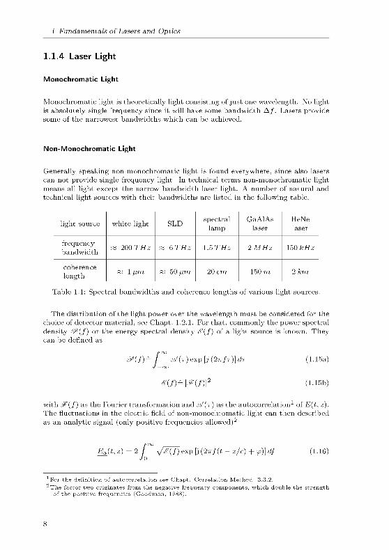
Monochromatic light is theoretically light consisting of just one wavelength. No lightis absolutely single frequency since it will have some bandwidth A/. Lasers providesome of the narrowest bandwidths which can be achieved.
Non-Monochromatic Light
Generally speaking non-monochromatic light is found everywhere, since also lasers
can not provide single frequency light. In technical terms non-monochromatic lightmeans all light except the narrow bandwidth laser light. A number of natural and
technical light sources with their bandwidths are listed in the following table.
light source white light SLDspectral
lamp
GaAlAs
laser
HeNe
laser
frequencybandwidth
as 200 THz as 6 THz 1 5THz 2 MHz 150 kHz
coherence
lengthm 1 ßm m 50 ßm 20 cm 150 m 2 km
Table 1.1 Spectral bandwidths and coherence lengths of various light sources.
The distribution of the light power over the wavelength must be considered for the
choice of detector material, see Chapt. 1.2.1. For that, commonly the power spectral
density £^(f) or the energy spectral density S(f) of a light source is known. Theycan be defined as
/oo s/(t) exp [j (2tt/t)] dr (115a)-OO
<T(/)=|^(/)|2 (115b)
with .S£(f) as the Fourier transformation and -s/{t) as the autocorrelation1 of E(t, z).The fluctuations in the electric field of non-monochromatic light can then described
as an analytic signal (only positive frequencies allowed)2
Ea(tt z) = 2 ^(TJexp [j (2irf(t - z/c) + tp)} df (1.16)Jo
For the definition of autocorrelation see Chapt Correlation Method 3 3 2
The factor two originates from the negative frequency components, which double the strengthof the positive frequencies (Goodman, 1988)
8
1.1 Electromagnetic Waves
Optical Coherence Temporal/Spatial3
In general one has to differentiate between two types of coherence, temporal coher¬
ence and spatial coherence. Temporal coherence means the ability of a light beam
to interfere (constructive optical mixing) with a delayed, but spatially not shifted,version of itself. Spatial coherence, on the other hand, means the ability of a lightbeam to interfere with a spatially shifted, but not delayed, version of itself. Allowing
temporal and spatially shifting together leads to the concept of mutual coherence.
A measure of coherence is provided by the definitions of the complex degree ofcoherence j(t), which represents a normalized version of the self coherence function,which in turn is the autocorrelation s/(t) of the analytic signal Ea(t, z)
^ = ^oy (L17)
According to Mandel (1959) the coherence Urne rc can be defined as
/oo h(r)\2dr (1.18)-oo
Furthermore, the coherence length lc is the distance which the light propagates
within the coherence time
lc = ctc (1.19)
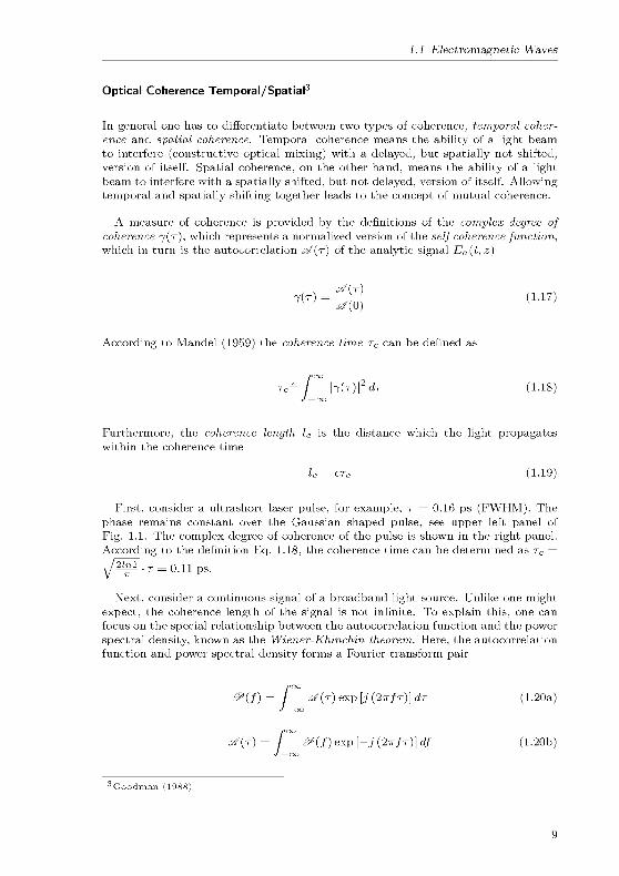
First, consider a ultrashort laser pulse, for example, r = 0 16 ps (FWHM). The
phase remains constant over the Gaussian shaped pulse, see upper left panel of
Fig. 1.1. The complex degree of coherence of the pulse is shown in the right panel.
According to the definition Eq. 1.18, the coherence time can be determined as rc =
/2!n20 n
Next, consider a continuous signal of a broadband light source. Unlike one might
expect, the coherence length of the signal is not infinite. To explain this, one can
focus on the special relationship between the autocorrelation function and the power
spectral density, known as the Wiener-Khmchm theorem. Here, the autocorrelation
function and power spectral density forms a Fourier transform pair
/oo s/(t) exp [j (2tt/t)] dr (1 20a)-CO
/CO &U) exp [-j (2tt/t)] df (120b)-oo
'Goodman (1988)
9

1 Fundamentals of Lasers and Optics
Corresponding to Goodman (1988) the complex degree of coherence in terms of
power spectral density can then be expressed as
/'OO
7(r)= / &(f) exp [-j (2ttfr)]dfJo
roo
with I &{f)df = 1
Jo
!p(f) is the normalized power spectral density, see lower left panel Fig. 1.1.
(1 21a)
(1 21b)
With Eq. 1.18 the coherence time of a broadband light source can now be expressedas a function of the frequency bandwidth A/
f3?
A/(1.22)
with f e? as a form factor of the spectral shape of the power density spectrum and
A/ as the FWHM bandwidth (half power bandwidth). In particular, f e? is 1 for a
rectangular, 0.318 for a Lorenzian and 0.664 for a Gaussian spectrum.4
time [ps]
04 05 06
optical delay [ps]
-03-02-01 0 01 02 03
frequency [THz]
239 236 233 230 227
«05
1260 1280 1300 1320
wavelength [nm]
-100 -50 0 50
[microns]
100
Fig. 1.1 Laser pulse, complex degree of coherence and power spectral density."
Please note the factor f^ given here is valid for energy fluctuations For intensity fluctuations
as measured by photoreceivers the square of fg& has to be considered
3For visualization the wavelength m the figure is scale up by a factor of 6 The duration of
the pulse was chosen such that the power spectral density is equivalent to that of SuperlumSLD-HP-56-HP (Fig 1 4)
10
1.2 Optical Components
For spatial coherence consider a non-monochromatic point source of zero diameter.
It emits temporal low coherence light, which on the other hand is highly spatiallycoherent. The light from a collection of incoherent point-sources instead would have
lower spatial coherence. If multiple point sources are coherent with each other, e.g.,
multiple slits in a Young's slit experiment, there is no loss of spatial coherence.
Spatial coherence can be increased with a spatial filter, i.e., a very small pinhole.The spatial coherence of light will also increase as it travels away from the source as
the source appears smaller (more pointlike) and the waves become more like a planewave.
1.2 Optical Components
1.2.1 Photodetectors
Fluctuations of the energy density of light waves cannot be measured directly. Usu¬
ally the photodetectors used for light detection do not have such high frequencyresolution because of the inertia of electron emission. Thus, a photodetector shows
an intensity fluctuation / as temporal average of the Poynting vector (Eq. 1.12). In
complex notation this leads to a simple mathematical representation for the electro¬
magnetic intensity
I r C£
I=tJ |P|dt=-E±-E^ (1.23)
T
The power detected on a photodiode includes furthermore the integration of Eq. 1.23
over the sensitive surface of the detector
Pp=ffldA (1.24)
A
The perpendicular symbols in Eq. 1.23 indicate that only components perpendicularto the detector's surface directly contribute to the electron emission. Other vec¬
tor components result in detector losses. The output of electric current is directly
proportional to the detected power
iv = Gq^-Pv (1.25)
with q as elemental charge, rjq as the quantum efficiency (a factor which considers
the detector's material properties), h as the Planck constant (after Max Planck
1858-1947) and / as the light frequency. In addition, the generated signal in a
photodetector is amplified, here accounted for by gain factor G.
Due to the time averaging behavior of the photodetector, all frequencies above
a certain cut-off frequency fc are represented as a DC current signal component.
11

1 Fundamentals of Lasers and Optics
Therefore the output current of a detector can be described by the sum of a DC
component and further AC parts
*P = !dc + %AG cos (<*>t + f) = »DC [1 + mcos (u>t + (p)] (1.26a)
1AG
1>DC(1.26b)
with m as the so-called modulation depth or visibility.
Technical Characteristics 6
Spectral Responsivity R\ The responsivity of a photodiode is a measure of the
sensitivity to light and it is defined as the ratio of the photocurrent ip to the received
light power Pp at a given wavelength:
Rx = (1.27)
In other words, it is a measure of the effectiveness of the conversion of the light powerinto electrical current, see Fig. 9.1. It varies with the wavelength of the incident lightas well as with the applied reverse bias and the temperature.
^ 0 30
g 0 60
m
= 0 40
0 20
0 00
BOO 1Q0D 1200 1400
Wavelength, urn
1600 1800
Fig. 1.2: Responsivity of a photoreceiver - Newport model 1811.
6UDT Sensors Inc. (2006)
12
1.2 Optical Components
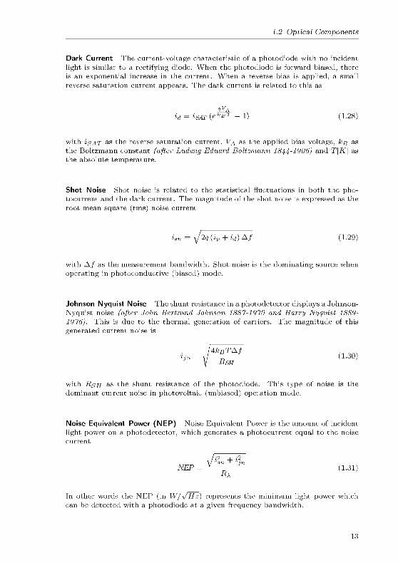
Dark Current The current-voltage characteristic of a photodiode with no incident
light is similar to a rectifying diode. When the photodiode is forward biased, there
is an exponential increase in the current. When a reverse bias is applied, a small
reverse saturation current appears. The dark current is related to this as
1VA
td = tSAT(ekBT _i) (1.28)
with isAT as the reverse saturation current, Va as the applied bias voltage, kg as
the Boltzmann constant (after Ludwig Eduard Boltzmann 1844-1006) and T[K] as
the absolute temperature.
Shot Noise Shot noise is related to the statistical fluctuations in both the pho¬tocurrent and the dark current. The magnitude of the shot noise is expressed as the
root mean square (rms) noise current
isn = ^J2q (ip + id) A/ (1.29)
with A/ as the measurement bandwidth. Shot noise is the dominating source when
operating in photoconductive (biased) mode.
Johnson-Nyquist Noise The shunt resistance in a photodetector displays a Johnson-
Nyquist noise (after John Bertrand Johnson 1887-1970 and Harry Nyquist 1889-
1976). This is due to the thermal generation of carriers. The magnitude of this
generated current noise is
•J»- iFff^ (1-30)
with Rsh as the shunt resistance of the photodiode. This type of noise is the
dominant current noise in photovoltaic (unbiased) operation mode.
Noise Equivalent Power (NEP) Noise Equivalent Power is the amount of incident
light power on a photodetector, which generates a photocurrent equal to the noise
current
V lln + V/
NEP = - — (1.31)Rx
V '
In other words the NEP (in W/\/Hz) represents the minimum light power which
can be detected with a photodiode at a given frequency bandwidth.
13

1 Fundamentals of Lasers and Optics
1.2.2 Optical Fibers 7
In the 1840's, the Swiss physicist Daniel Gollodon and the French physicist J JacquesBabmet showed that light can be guided along jets of water. In 1854, John Tyndall,a British physicist, popularized light guiding in a demonstration, guiding light in a
jet of water flowing from a tank to another. As water poured out through the spout
of the first container, Tyndall directed a beam of sunlight at the path of the water.
Due to the effect called internal reflection, the light seen by the audience followed
a zigzag path inside the curved path of the water. By the turn of the century,
inventors realized that bent quartz rods could carry light, and patented them as
dental illuminators.
Heinrich Lamm as medical student in Munich demonstrated image transmission
through a bundle of optical fibers. His goal was to look inside inaccessible parts
of the body. In a 1930 paper he reported on transmitting a image of a light bulb
filament through a short bundle. A crucial innovation was made by Abraham van
Heel in 1954. He first covered a bare fiber with a transparent cladding of a lower
refractive index. This protected the total reflection surface from contamination and
greatly reduced crosstalk between fibers. Since then fiber optic research has led to
a dramatic improvement in light guiding performance and fibers are used today in
a wide field of applications, especially in telecommunication and medicine.
Basically, optical fibers are classified into two types, single mode fibers and multi-
mode fibers. Furthermore, fibers may be categorized as step-index or graded-indexfibers.
Multimode Step-Index Fiber
Fig. 1.3 shows the principle of total internal reflection in a multimode step-indexfiber. Because the index of refraction of the fiber core is higher than that of the
cladding, light within the numerical aperture (NA) can enter the fiber and is then
guided along. The numerical aperture of a step-index fiber can be described as
NA = n0 sin 9A = n0 Jn\ - n\ (1-32)
with n\ and ni as the refractive indicies of the fiber's core and cladding media and
no as the refractive index of the surrounding medium, which normally is air with
no ~ 1. For a multimode fiber, different light modes can be transmitted. The
different modes enter the fiber at different angles and then each mode for itself
bounces back and forth by total internal reflection (see Fig. 1.3). It can be seen that
the different modes travel different distances inside the fiber, causing the two modes
to arrive at separate times. This disparity between arrival times of the different light
rays is known as dispersion, and the result is a distorted signal at the receiving end.
This is especially important for interferometry applications, see Chapt. 2.2.2.
Hecht (2006) and Force Inc (2006)
14

1.2 Optical Components
Step fm$e.x
(hfuitimtd*s)
Cladding Coie.
"V ..-"^ Ravs
Gmd^d Index
(Multimode)
© V*" ^c" Vf" Vf^ ^*>
Single Mods
(Manonmde)
Fig. 1.3: Types of optical fibers.
Multimode Graded-lndex Fiber
Graded-index refers to the fact that the refractive index of the core gradually de¬
creases from the center of the core
NA(r) = no sinda = yn\(r) (1.33)
As Fig. 1.3 shows, the light rays no longer follow straight lines. Instead they follow
a serpentine path being gradually bent back towards the center by the continuously
varying refractive index. This reduces the arrival time disparity because all modes
arrive at about the same time. The modes traveling in a straight line are in a regionof higher refractive index, so they travel more slowly than the serpentine modes.
These travel farther but faster in the lower refractive index of the outer core region.
Singlemode Fiber
As the core radius of a fiber decreases, the number of possible propagation modes
decreases, too (see Fig. 1.3). With a core radius of about 3..10 /im, singlemode fibers
allow only one mode to propagate. Dependent on the wavelength, the number of
modes carried is described by the so called V-parameter
frrreore
A(1.34)
The number of modes which can enter the fiber is approximately V2. The smaller
core diameter of singlemode fibers makes coupling light into the core more diffi-
15

1 Fundamentals of Lasers and Optics
cult. Similarly, the tolerances for singlemode connectors and splices are much more
demanding.
An additional important variety of singlemode fiber is the polarization maintaining
(PM) fiber. The PM fiber is designed to guide only one polarization of the input
light. Next the core, there are two additional filaments called stress rods. These
stress rods create stress in the core of the fiber such that the transmission of onlyone polarization plane of light is favored.
1.2.3 Optical Gratings and Bragg Cells
Optical gratings and Bragg cells are often used as beamsplitters, modulators or
frequency shifters. In laser Doppler systems frequency shifting gives the possibility to
determine the direction of the flow velocity. Kerr cells or Pockels cells are also feasible
as frequency shifting devices, but due to the limited quality, frequency variations and
low frequency shift, they have not become common in laser Doppler applications.
Diffraction Grating
For diffraction through a slit the intensity of the diffracted light can be expressed as
T sin2 ( ^r- (sin/3D — sin a) ]^
=^ y~ (1 35a)
/0 (fx(sin/3p-sina))
sin/3p = sin a ±—, p = 0, 1, 2 (135b)
where a is the incidence angle, ßp the diffraction angle of order p and b the gratingwidth. The assumptions are that the source and the receiver are far away from the
grating, the grating length I is much larger than its width b, that b is larger than two
times the wavelength b > 2A and the amplitude or phase changes across the grating
are sinusoidal. The incidence angle here changes only the position of the intensity
maximum.
If the grating is moving perpendicular to the incident light (a = 0), the diffracted
light experiences a Doppler frequency shift, see Chapt. 3.2.1.
8AA-Opto-Eelectromc (2003)
16

1.2 Optical Components
Bragg Cells
A Bragg cell creates a phase grating with acoustically generated pressure waves
within a crystal. A so-called quality factor Q defines the interaction regime between
the acoustic and light waves (AA-Opto-Eelectronic, 2003)
(1.36)
with A as the light wavelength, A as the acoustic wavelength, n as the refractive index
of the crystal and I as the length over which the light wave interacts with the acoustic
wave. For Q << 1 and Q >> 1 two interaction regimes can be distinguished.
Raman- Nath regime For Q << 1 the light roughly normal to the acoustic waves
is diffracted into several orders ( , —2, —1, 0, 1, 2, ) with an intensity given by the
Bessel function.9
Bragg regime For Q >> 1 the light has to be at a certain incidence angle. Onlythen the light is refracted optimally at its 1st order with twice the incidence angle,the other orders are annihilated by destructive interference.
1.2.4 Superluminescent Light Emitting Diodes (SLD's)
The special property of superluminescent diodes (SLD's)10 is the combination of
laser-diode-hke output power with a broadband optical spectrum. The large band¬
width translates into a short coherence length allowing SLD's to be used as low
coherence interferometry light sources (see Chapt. 2.2). The small form factor and
user friendly operation make them advantageous. High power SLD's have first been
developed in 1989 by Gerard A. Alphonse, Alphonse et al. (1988).
SLD's are based on a p-n-junction embedded in an optical waveguide. When biased
electrically in the forward direction they show optical gain and generate amplified
spontaneous emission over a wide range of wavelengths. They are designed to have
high single pass amplification, but unlike laser diodes, the feedback is insufficient
to perform lasing action. A rejection of the cavity modes is typically achieved by
tilting the waveguide with respect to the end facets and with anti-reflection coatings
at the facets. Thus a smooth broadband spectrum, which is temporally incoherent,
Chandrasekhara Venkata (C V ) Raman (1888-1970) In 1930 Raman was awarded the Nobel
prize m physics for his 1928 discovery of the Raman Effect, which demonstrates that the
energy of a photon can undergo partial transformation withm matter In 1934-36, with his
colleague Nagendra Nath, Raman proposed the Raman-Nath Theory on the diffraction of light
by ultrasonic waves He was director of the Indian Institute of Science and founded the Indian
Academy of Sciences m 1934 and the Raman Research Institute m 1948 (Coutsoukis, 2006)Please note frequently used acronyms for the superluminescent diode are SLD and alternative
SLED However, SLED is not recommended, because it is more often used for surface-emitting
LED, l e,with a totally different meaning
17
1 Fundamentals of Lasers and Optics
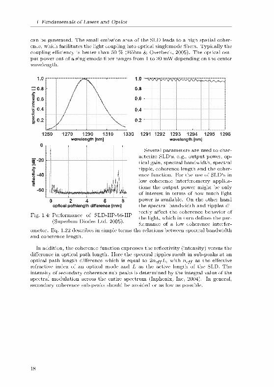
can be generated. The small emission area of the SLD leads to a high spatial coher¬
ence, which facilitates the light coupling into optical singlemode fibers. Typically the
coupling efficiency is better than 50 % (Böhm & Overbeck, 2005). The optical out¬
put power out of a singlemode fiber ranges from 1 to 30 mW depending on the center
wavelength.
1.0
= 0.8
ë
I"I 0.4
I 0,2
1250 1270 1290 1310
wavelength [nm]
1330 1291 1292 1293 1294
wavelength [nm]
12S5 1296
2--202,
1„„
f,-40
-60
0 2 4 6 8
optical pathlength difference [mm]
Fig. 1.4: Performance of SLD-HP-56-HP
(Superlum Diodes Ltd, 2005).
ometer. Eq. 1.22 describes in simple terms the relations between spectral bandwidth
and coherence length.
Several parameters are used to char¬
acterize SLD's, e.g., output power, op¬
tical gain, spectral bandwidth, spectral
ripple, coherence length and the coher¬
ence function. For the use of SLD's in
low coherence interferometry applica¬tions the output power might be onlyof interest in terms of how much light
power is available. On the other hand
the spectral bandwidth and ripples di¬
rectly affect the coherence behavior of
the light, which in turn defines the per¬
formance of a low coherence interfer-
In addition, the coherence function expresses the reflectivity (intensity) versus the
difference in optical path length. Here the spectral ripples result in sub-peaks at an
optical path length difference which is equal to 2neffL, with rae// as the effective
refractive index of an optical mode and L as the active length of the SLD. The
intensity of secondary coherence sub-peaks is determined by the integral value of the
spectral modulation across the entire spectrum (Inphenix, Inc, 2004). In general,
secondary coherence sub-peaks should be avoided or as low as possible.
18

2 Interferometry
Interferometry relies on the principles of interference to determine properties of
waves, their sources, or the wave propagation medium. Interference is understood as
the superposition of two or more waves. When waves moving along their direction of
propagation, either from one source using different paths or from different sources,
reach the same point in space at the same time, interference occurs. If the waves
arrive in-phase (the crests arrive together), constructive interference occurs. The
combined crest is an enhanced version of the one from the individual wave. When
they arrive out-of-phase (the crest from one wave and a trough from another), de¬
structive interference cancels the wave motion. Please note the energy of the wave
is not lost, it moves to areas of constructive interference.
Acoustic interferometry has been applied to study the velocity of sound in a fluid.
Radio astronomers use interferometry to obtain accurate measurements of the po¬
sition and properties of stellar radio sources. Optical interferometry is widely used
to observe objects without touching or otherwise disturbing them. Interpreting the
fringes reveals information about optical surfaces, the precise distance between the
source and the observer, spectral properties of light, or the visualization of processes
such as crystal growth, combustion, diffusion or shock wave motion.
The most striking examples of interference occur in visible light. Interference of
two or more light waves appears as bright and dark bands called "fringes." Inter¬
ference of light waves was first described in 1801 by Thomas Young (1773-1829)when he presented information supporting the wave theory of light. The observa¬
tion and explanation of interference fringes in general dates back to Robert Hooke
(1635-1703) and Isaac Newton (1643-1727). Nevertheless the invention of interfer¬
ometry is widely attributed to the American physicist Albert Abraham Michelson
(1852-1931).
It is important to note that almost every observation of interference is time aver¬
aged. Thus, interfering waves must be coherent, i.e., they need to have a predictable
phase relationship. Otherwise, for random phase changes between two waves, the
interference signal is destroyed.
2.1 Michelson-lnterferometer
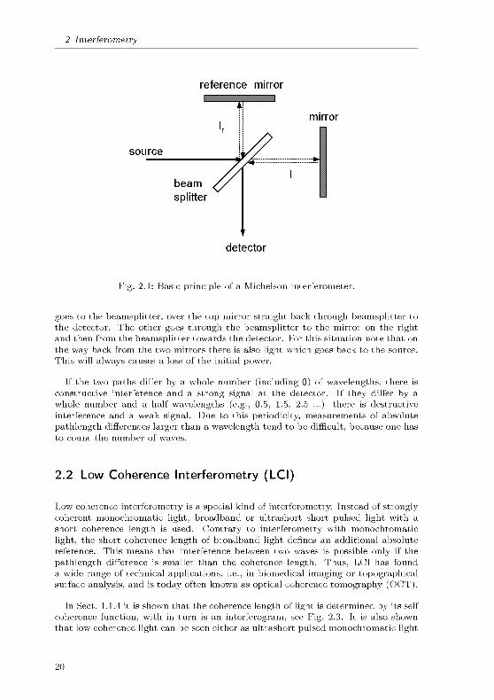
A very common example of an interferometer is the Michelson (or Michelson-Morley)type (after Albert Michelson (1852-1931) and Edward Williams Morley (1838-1923)). The basic building blocks are a light source (or matter source), a detector,two mirrors and one semitransparent mirror (often called beamsplitter), arranged as
shown in Fig. 2.1. There are two possible paths from the source to the detector. One
19
2 Interferometry
reference mirror
mirror
source
beam
splitter
detector
Fig. 2.1 Basic principle of a Michelson interferometer.
goes to the beamsplitter, over the top mirror straight back through beamsplitter to
the detector. The other goes through the beamsplitter to the mirror on the rightand then from the beamsplitter towards the detector. For this situation note that on
the way back from the two mirrors there is also light which goes back to the source.
This will always causes a loss of the initial power.
If the two paths differ by a whole number (including 0) of wavelengths, there is
constructive interference and a strong signal at the detector. If they differ by a
whole number and a half wavelengths (e.g., 0.5, 1.5, 2.5 ...) there is destructive
interference and a weak signal. Due to this periodicity, measurements of absolute
pathlength differences larger than a wavelength tend to be difficult, because one has
to count the number of waves.
2.2 Low Coherence Interferometry (LCI)
Low coherence interferometry is a special kind of interferometry. Instead of stronglycoherent monochromatic light, broadband or ultrashort short pulsed light with a
short coherence length is used. Contrary to interferometry with monochromatic
light, the short coherence length of broadband light defines an additional absolute
reference. This means that interference between two waves is possible only if the
pathlength difference is smaller than the coherence length. Thus, LCI has found
a wide range of technical applications, i.e., in biomedical imaging or topographicalsurface analysis, and is today often known as optical coherence tomography (OCT).
In Sect. 1.1.4 it is shown that the coherence length of light is determined by its self
coherence function, with in turn is an interferogram, see Fig. 2.3. It is also shown
that low coherence light can be seen either as ultrashort pulsed monochromatic light
20

2.2 Low Coherence Interferometry (LCI)
or equivalently as broadband light. For the latter there is a fixed mathematical
relationship between the power spectral density and the self coherence function,which is known as the Wiener-Khmchm theorem. Physically, one might regardcontinuous emitted broadband light also as pulses, but instead of the light amplitude,its phase changes pulsewise by a random value. For a time averaged interferogramthis means also loss of coherence.
2.2.1 Principle
As mentioned low coherence interferometry basically does not differ in the designof the optical components from a classical interferometer. Only the monochromatic
and coherent light source is replaced by a light source with certain short coherent
light pulses. Consider the upper mirror in Fig. 2.1 as a reference, where the distance
dr = 2lr to the beamsplitter is known. The right mirror instead is located at
an unknown distance d. The reference mirror can be moved back or forth until
interference occurs. Since interference can only be observed if the optical path
length difference (twice the distance to the beamsplitter) of the reference and the
second mirror is within the coherence length of the light source, the position of the
second mirror is hence known by the position of the reference mirror (see Fig. 2.2)
d = dr
\{d-dr)\ = 2\{l-lr)\ < lc
(2 la)
(2 1b)
Replacing the second mirror by an object to be investigated, gives rise to various
LCI applications such as, for example surface profilometry.
a)AAA y\AA
beamsplitter 21 > 21+1
M AAA
detector
beamsplitter
AAA
2lr=2ldetector
c)A"A AAA
beamsplitter 2lr<2l-lcdetector
Fig. 2.2 Low coherence interferometry principle a) path of reference wave (bold)too long c) path of reference wave to short b) pathlength difference of both
waves is within the coherence length, i.e., interference occurs.
21
2 Interferometry
To make possible interference visible on the detector, one light beam in the interfer¬
ometer can be shifted in its frequency. Following the optical wave mixing equations
Eqs. 1.14 in Chapt. 1.1.3, the sum of two equal waves with the same phase, polar¬
ization, pathlength and propagation direction, but with a different amplitude and
frequency can be expressed as
E = Ej + E2 = Ei exp [j (wit - kz)] + E2 exp [j {uj2t - kz)] (2.2)
According to Eq. 1.23 the averaged intensity is then
I = —E-E* = — [El +E| +2E1E2cos{uj2t - uJit)] (2.3)
This equation can be split into two parts, one corresponding to the DC term and
one to the AC components of the intensity
IDC =
y (E2 + El) (2 4a)
IAC = ceE1E2 cos ( Aojt) (2 4b)
If the frequency difference Alo of the AC part is within the detector's frequency
bandwidth, the output current on the detector is similar to Eqs. 1.26
*P = !dc [1 + mcos (Awt)] (2.5)
with Alo as the frequency of the beat note representing an indicator for interference.
Thus, one can focus on the intensity of the beat note to recover the envelope of
an interferogram. Delaying the reference reflection in an interferometer from dr <
(d — lc) to dr > (d + lc), the beat note intensity can be recorded. As an exam¬
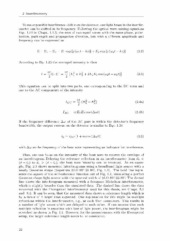
ple, Fig. 2.3 shows measured interferograms using a broadband light source with a
nearly Gaussian shape (Superlum SLD-HP-56-HP, Fig. 1.4). The bold line repre¬
sents the square of the self-coherence function out of Fig. 1.1, simulating a perfectGaussian shape light source with the spectral width of SLD-HP-56-HP. The dotted
line shows the interferogram measured with a freespace Michelson interferometer,which is slightly broader than the simulated data. The dashed line shows the data
recovered with the fiberoptical interferometer used for this thesis, see Chapt. 5.1
and 8.2. It can be seen, that the measured data shows a coherence length which is
by a factor of 4 larger than expected. One explanation for this might be multiplereflections within the interferometer, e.g., at each fiber connectors. This results in
a number of light waves which are delayed to each other. If one assume that each
multiple reflection is associate with loss of light power, the interferogram might be
stretched as shown in Fig. 1.1. However, for the measurements with the fiberoptical
setup, the larger coherence length needs to be considered.
22
2.2 Low Coherence Interferometry (LCI)
1
09
08
07
„
06
w 05c
s-
04
03
02
0 1
/->
/
1
1
J
1
1
1
/
1
1
1
{ \J ;/
/ .7
W \~
\
\
\
\
\
\
\
\
\
\
N
i". \
V v
v x
V x-
-200 -150 -100 -50 0 50
optical delay [microns]
100 150 200
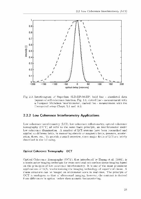
Fig. 2.3 Interferogram of Superlum SLD-HP-56-HP bold line - simulated data
(square of self coherence function, Fig. 1.1, dotted line - measurement with
a freespace Michelson interferometer, dashed line - measurement with the
fiberoptical setup Chapt. 5.1 and 8.2.
2.2.2 Low Coherence Interferometry Applications
Low coherence interferometry (LCI), low coherence reflectometry, optical coherence
tomography (OCT) all refer to the same basic principle, an interferometer under
low coherence illumination. A number of LCI systems have been researched and
applied to different fields, in measuring electric or magnetic fields, pressure, acceler¬
ation, flows, etc.. To provide a small overview, three major fields of LCI are brieflydescribed in the following.
Optical Coherence Tomography - OCT
Optical Coherence Tomography (OCT), first introduced by Huang et al. (1991), is
a noninvasive imaging technique for cross-sectional sub-surface tissue imaging based
on the principles of low coherence interferometry. It is one of the most prominent
applications of LCI, revolutionizing the imaging technology of superficial tissue. A
tissue structure can be imaged on micrometer scale in real time. The principle of
OCT is analogous to that of ultrasound imaging, however, the contrast is derived
from differences in optical rather than acoustic backscattenng.
23

2 Interferometry
Optical Low Coherence Reflectometry - OLCR
Optical low coherence reflectometry (OLCR) is an interferometne technique that
allows one to measure the amplitude and relative phase of reflected light. The tech¬
nique was originally developed for reflection measurements in telecommunications
devices with micrometer resolution. There, optical interfaces in complex structures
can be precisely located and measured. The principle is based on coherent cross-
correlation detection of light reflected from the sample. OLCR has also applicationsin medicine, e.g., for corneal thickness determination (Masters, 1999).
Distributed Laser-Doppler Velocimetry - DLDV
Distributed laser-Doppler velocimetry (DLDV) is a technique using low coherence
interferometry for flow velocimetry. The technique was first presented by Gusmeroh
& Martinelli (1991). It permits continuous interrogation of the flow velocity in any
point belonging to a collimated laser beam. The technique can be seen as a specialform of reference beam laser-Doppler velocimetry, see Chapt. 3.2.2.
DLDV uses low coherence light together with a Michelson interferometne con¬
figuration. The flow is illuminated by a collimated light beam. The position of
the measurement volume can be chosen everywhere within the collimated beam, by
setting the position of the reference within the interferometer. The size of the mea¬
surement volume depends on the beam diameter and the coherence length of the
light source. Among the many particles crossing the sensing beam, only the parti¬
cles within the coherent volume produce a interference signal. The flow velocity is
determined by reference beam LDV frequency analysis.
24
3 Laser Velocimetry
3.1 Light Scattering of Small Particles
Optical flow velocimetry techniques are often based on the detection of the move¬
ment of small particles in the fluid, so-called seeding particles. The basic assumption
is that the small seeding particles follow the fluid, thus representing the flow. How¬
ever, this is also one major cause for measurement errors. The mass of the seedinginvolves an inertia, which leads to a delayed reaction of the particles in the flow
field. Particularly for investigations in shock dynamics this is an essential issue. The
smaller the particles the better is their ability to follow the flow, but also the lower
is the intensity of the scattered light.
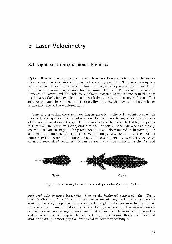
Generally speaking the size of seeding in gases is on the order of microns, which
means it is comparable to optical wavelengths. Light scattering off such particles is
characterized as Mie-scattenng. Here the intensity of the backreflected light dependsnot only on the particle's shape, diameter and refractive index, but also and mostlyon the observation angle. The phenomenon is well documented in literature, but
also relative complex. A comprehensive summary, e.g., can be found in van de
Hülst (1981). To give an example, Fig. 3.1 shows the general scattering behavior
of micrometer sized particles. It can be seen, that the intensity of the forward
Fig. 3.1 Scattering behavior of small particles (Schodl, 1991).
scattered light is much larger than that of the backward scattered light. For a
particle diameter ds > 2A, e.g., it is three orders of magnitude larger. Sidewards
scattering strongly depends on the observation angle, and sometimes there is almost
no scattering. Thus optical setups where the light source and the receiver are on
a line (forward scattering) provide much better results. However, most times the
optical access makes it impossible to build the system this way. Hence, the backward
scattering setup is most popular for optical velocimetry techniques.
25
3 Laser Velocimetry
3.2 Laser-Doppler Systems
3.2.1 The Doppler Effect
The Doppler effect (after Christian Andreas Doppler 1803-1853), is the apparent
change in frequency or wavelength of a wave that is perceived by an observer moving
relative to the source of the wave. For waves which do not require a medium (suchas light waves) only the relative difference in velocity between the observer and the
source needs to be considered.
It is important to realize that the frequency which the source emits does not
actually change. Consider the following simple analogy. A person A throws one
ball every second to a second person B. Assume that the balls travel with constant
velocity. If A is stationary, B will receive one ball every second. However, if A is
moving towards B, B will receive the balls more frequently, because there will be
less spacing between the balls. The same is true if A is stationary and B is moving
towards A. On the other hand the spacing between the balls increases, if A or B
move away from each over. So it is actually the wavelength which is affected, and
as a consequence, the perceived frequency too.
More generally the result in change of wavelength and frequency of electromagneticwaves can be expressed with
/ « /o (l - ^) (3.1)
with \vr\ << c, / as the light frequency detected by a receiver, /o as the frequencyof the light source, c as the specific speed of light and vr as the relative velocitybetween the source and the observer. The relative velocity is denoted positive, if the
source and the observer are moving away from each other.
3.2.2 Laser-Doppler Velocimetry - LDV
Laser-Doppler velocimetry is a technique to obtain velocity data using the Dopplereffect. In the field of flow analysis it is an indirect measurement technique, since it
measures the velocity of inhomogeneities in the flow, so-called seeding particles.
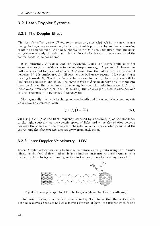
Fig. 3.2 Basic principle for LDA techniques (direct backward scattering).
The basic working principle is illustrated in Fig. 3.2. Due to that the particle acts
both as a moving receiver and as a moving emitter of light, the frequency shift as a
26

3.2 Laser-Doppler Systems
result of the Doppler effect appears twice. The frequency shift as an equivalent of
the particle velocity is then described by
fshift ~ foil j - /o
sxnct
= -2-^—-vp (3.2)Ao
with c = / • A and \vp\ << c as the particle velocity. Please note that the equation is
only valid for LDA m direct backward scattering. The frequency shift will be positive
for particles moving m laser direction.
For typical flows the Doppler shift is in the order of W6Hz, which is very small
compared to the frequencies of light of approximately W14,Hz. Thus a direct mea¬
surement of the Doppler shift tends to be impossible, since the cut-off frequenciesof common photoreceivers are around W9Hz. However, e.g., with the help of an
interferometer or the use of frequency dependent absorption cells the small Dopplershifts can be detected. Absorptions cells are often used for Doppler global velocime¬
try (DGV). The signal is then an intensity value which corresponds to a frequencyshift or the velocity data, respectively.
LDV - Doppler Difference Method
Fig. 3.3 shows a schematic of a LDV dual-beam configuration, also known as Dopplerdifference method. For this the output from a laser is split into two beams. Both
beams are focused onto the same point to form one measurement volume. Lightscattered from this region can be collected by another focusing lens. Thus, reflec¬
tions from both beams are then mixed on a detector surface. Analogous to Eq. 3.2
the Doppler shift appears twice, but for both of the beams. Following Eq. 1.14
(Chapt. 1.1.3) and Eq. 1.23/ 1.26 (Chapt. 1.2.1) the photoreceiver signal can be
expressed as
tP = %DC + iAC cos {ujt) (3.3)
wherein the AC part includes the frequency difference between the Doppler shifts of
the two beams. Thus, the system is sensitive to velocities orthogonal to the bisector
of the two incident beams
vp =-A^_
•
flM1(3-4)
2sin&/2 cosa
This equation is valid for either backward scattering or forward scattering setups.
LDV - Reference Beam Method
The reference beam LDV configuration was the first reported by Yeh & Cummins
(1964). In the reference beam technique light scattered from one illuminating beam
is collected and mixed with a reference beam on a photodetector. A simple schematic
27

3 Laser Velocimetry
incident waves
measurement volume
particle
Fig. 3.3: LDA dual-beam configuration.
of this configuration is shown in Fig. 3.4. In a Michelson interferometer configurationthe output from a laser diode is split by a beam splitter to form the signal and refer¬
ence beam. One output is focused to form the measurement volume. Light scattered
from this region is collected by the same lens. The reference beam is reflected bya plane mirror. Both backreflected beams are recombined at the beamsplitter and
heterodyned on a photodiode.
plane mirror
particles in
the focus
Fig. 3.4: Basic principle LDV - reference beam method.
The Doppler shift depends on the incident angle to the flow direction and on the
velocity of the flow. The flow velocity in backward scattering setup can hence be
expressed as
vp — „
'
JshzftIsvaoL
(3.5)
28
3.3 Laser-2-Focus Systems (L2F)
with a as the incident angle to the flow. In a forward scattering configuration, the
Doppler shift is of opposite sign.
3.3 Laser-2-Focus Systems (L2F)
3.3.1 Principle
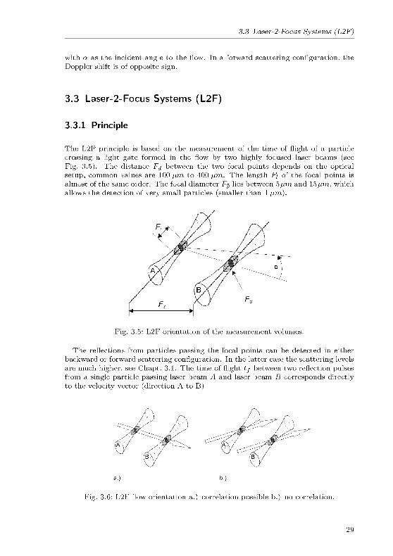
The L2F principle is based on the measurement of the time of flight of a particle
crossing a light gate formed in the flow by two highly focused laser beams (seeFig. 3.5). The distance Fj between the two focal points depends on the optical
setup, common values are 100 ßm to 400 ßm. The length Fi of the focal points is
almost of the same order. The focal diameter F$ lies between 5ßm and 15 ßm, which
allows the detection of very small particles (smaller than 1 ßm).
Fig. 3.5: L2F orientation of the measurement volumes.
The reflections from particles passing the focal points can be detected in either
backward or forward scattering configuration. In the latter case the scattering levels
are much higher, see Chapt. 3.1. The time of flight tf between two reflection pulsesfrom a single particle passing laser beam A and laser beam B corresponds directlyto the velocity vector (direction A to B)
a) b)
Fig. 3.6: L2F flow orientation a.) correlation possible b.) no correlation.
29

3 Laser Velocimetry
UABFd
(3.6)
Reflection pulses in a L2F setup can be classified into correlated and uncorrelated
events. Correlated double-pulses are from a single particle passing beam A and
B. The corresponding velocities vary around a certain mean value with a distorted
Gaussian distribution, whose variance correlates with the degree of turbulence. Since
correlated events are only possible if a particle may pass both beams, the orientation
of the light gate has to match with the flow direction, see Fig. 3.6. Otherwise onlyuncorrelated events from reflections of different particles will be detected, uniformlydistributed over the measurement time.
To characterize a full flow, generallya series of measurements has to be done
at different orientations within the an¬
gular range where correlated events are
expected. The statistical analysis will
result in a three-dimensional Gaussian
distribution curve in terms of angle and
velocity, see Fig. 3.7. The maximum of
this distribution curve then defines the
velocity vector u in the absolute coor¬
dinate system.
In order to distinguish between cor¬
related and uncorrelated events two
analysis methods are common, the cor¬
relation method and the histogrammethod.
Fig. 3.7: 3D distribution curve of a L2F
measurements series.
3.3.2 Correlation Method
The correlation method determines the analogy function of signals, the correla¬
tion function respectively. One distinguishes between auto-correlation and cross-
correlation. The auto-correlation function gives a value for the self-similarity of a
signal (only one detector is used for the beams A and B). The cross-correlation
instead gives a value for the similarity between two signals. The auto-correlation is
built by the integral of the product of a signal s(t) and the same but shifted signal
s(t + r)
/OO s(t)s(t + r)dt-OO
(3.7)
For the cross-correlation s(t + r) must be replaced by a second signal g(t + r). In
case of a time dependent measurement, the maximum of the correlation functions
can be attributed to the temporal shift within s or between s and g.
30

3.3 Laser-2-Focus Systems (L2F)
In technical use the integral can be discretized with / elements at time steps of rs
<^(rs) = ~^2 s(i)s(i + ts) for ts = 0. (3.8)
This equation gives good correlation results if either the number of elements or the
event rate are high enough. An increase of the time steps also gives better correlation
values, but causes a trade off in the temporal resolution. Thus, in the majority of
cases the correlation method is only used at high event rates (high particle seeding).
The time of flight, as a measure of the flow velocity, can be determined by the
position of peaks in the correlation function.
3.3.3 Histogram Method
The histogram method produces a frequency distribution of k time delays between
single particle pulses, which directly corresponds to the velocity. One divides the
time axis in a certain number of intervals Ai,..., An, so-called classes. Every velocitycan then attributed to a class Aj(l < j < n). The respective quantity Q3 of
velocities in a class is the so-called class occurrence. Dividing Q} by the number
k of velocity spot samples gives the relative class occurrence. The uncorrelated
velocities, statistically uniformly distributed, build the noise level of the velocity
histogram. The correlated velocities are related to a Gaussian curve (see Fig. 3.8).It directly represents the statistical behavior of the flow situation.
nUJiMfulfllii ,ii uliJilintLltlllBU fcUnBJift.y|time of flight classes [s]
Fig. 3.8: Statistical distribution of a L2F measurement at a fix angle.
The drawback of this method lies in the determination of the time delays between
the pulses. In a highly seeded flow the probability increases that several particlesare in the light gate at the same time. This creates an unproportional increase of
faster velocities. In addition it also makes a simple determination of the pulse delays
impossible. Thus this method is often used at low event rates, like in syntheticallyseeded flows.
31

3 Laser Velocimetry
32

Part II
Tip Clearance Probe
33

Introduction and Motivation
A turbine rotor must have a small but finite clearance to its surrounding casing.
This tip clearance is typically about one percent of the blade span. The leakage
flows, i.e., fluid flowing through the gap between the blade tips and the shroud of a
turbine or compressor, have large effects on the aerodynamics of the machinery and
are responsible for a significant percentage of overall losses in turbines (Sieverding,1985). Due to different thermal expansion coefficients and heating rates in the
turbine rotor and the machine casing, the tip clearance is not constant, but dependson the operating condition and varies during machine start-up and shut-down. In
order to increase the turbine efficiency, the tip clearance has to be as small as possible,while avoiding damage by blades touching the casing. Therefore, it is important to
measure and monitor the tip clearance under operating conditions.
Current tip clearance probes are mostly of inductive or capacitive type, with
typical relative accuracies of about 5 % (Sheard et al., 1999, Steiner, 2000). This
is sufficient in situations where the probe can be mounted flush with the turbine
casing, because the absolute errors are then small. In harsh and high-temperature
environments, such as in the early stages of gas turbines, this mounting scheme is not
feasible. The Curie point of rare earth metals, which is well below operating temper¬
atures in turbines, sets an upper bound on the maximum operation temperature of
these classical sensors (Barranger & Ford, 1981, Dhadwal & Kurkov, 1999). Probes
can be mounted in a cooled recess within the casing, but techniques are requiredwith sufficient absolute accuracy over the increased total distance (tip clearance +
recess). Optical measurement probes can provide the required resolution and are
generally not affected by temperature effects, e.g., (Barranger & Ford, 1981, Pfister
et al., 2005). Although the implementation of sensitive optical parts within the tur¬
bine is challenging, operating temperatures up to 900 K have been reported (Rooth& Hiemstra, 2001). Also microwave type clearance sensors (Geisheimer et al., 2004)were reported to operate at high temperatures.
A new approach based on optical low coherence interferometry is reported here.
The novel tip clearance probe yields near real-time, blade-to-blade tip clearance
data with absolute measurement errors in the order of tens of microns even in harsh
environments with limited optical access. The measurement technique relies on
the interference between backreflected light from the blade tips during the blade
passage time and a frequency shifted reference. Due to the measurement principle the
absolute spatial accuracy only depends on the coherence length of the light source,
rendering the system insensitive to the measurement distance, turbine vibrations
and large temperature changes. For typical scenarios where the tip clearances are
within a range of a few millimeters, the technique can yield data once every second
for each blade. This allows to monitor transient effects during turbine start-up
and shut-down. Optical access is provided by a single optical fiber of arbitrary
length. The robust sensor head can easily be mounted in a cooled recess. Its own
35

maximum operating temperature is about 1000 K. The high operating temperature
of the sensor itself together with additional cooling possibilities allow the use of the
system in environments with temperatures which are much higher, but standard in
today's gas turbines. The sensitive mechanical, electronic and optical components
of the system are placed far from the turbine in a separate post-processing unit.
The presented prototype of such a system is an all-fiber assembly, with self-
calibrating capabilities and a spatial resolution of less than 50 /im. The data ac¬
quisition system consists of a digital storage oscilloscope and a common PC. The
limited data transfer rates of this system lead to reduced scan rates (typically one
per minute). Results from proof-of-pnnciple measurements at different turbines,the LISA test facility at ETH Zurich and the GT26 gas turbine at ALSTOM, are
reported in this thesis.
36

4 Turbomachinery Background
4.1 Tip Clearance/Leakage Flows
The clearance between the tip of the rotating components (compressor or turbine
blades) and the shroud is inevitable in turbine engines. The leakage flow across
this gap is caused by the pressure difference between the pressure side and suction
side of the blade. This flow can have significant effects on the stage aerodynamic
performance and on the structural durability of the blade. In the case of hot gas
turbines the special flow situation across the blade tip can result in hot spots in this
blade region. Therefore, different cooling schemes, e.g., film cooling, are applied to
improve the durability of the components.
The leakage flow tends to roll up to form vortices beginning at the blade tips, see
Fig. 4.1. The interaction of this secondary flow with the main flow causes complexflow phenomena with many of detrimental effects on the performance of an axial
turbine. The induced complex three dimensional flow field can span up to 20% of
the blade beginning at the tip.
Horae-Shoa Vortex Hubwall Passago Vortux
Fig. 4.1: Secondary flow field of an axial-turbine stage (Sjolander, 1997).
37

4 Turbomachinery Background
4.2 Clearance Effects in Turbines
As mentioned the secondary flows caused by the gap between blade tip and turbine
casing can have large impacts on the turbine operation and its efficiency. A whole
research field is occupied with the analysis and simulation of this complex issue. Two
of the main and obvious effects are loss generation and the change of heat transfer.
4.2.1 Losses
Tip clearance losses are responsible for a large fraction of the overall loss in a turbine.
The average loss level is about 25% of the total loss and 33% of rotor loss. As an
example, Fig. 4.2 shows the percentage of losses for different effects in comparison to
the total loss of several turbines (13-CYL, 13-CONE, 12, etc.). It can be seen that
even small changes in the tip clearance have direct effects on the turbine efficiency.
PKHCTEB IfFKHNCY U50 US DUS MIS «( 0919 0116 WW IJÎ3
Fig. 4.2 Sources of turbine losses (Booth, 1985b).
A conceptual model (see Fig. 4.3) shows that not only the reduced area of the blade
lowers the efficiency, but that leakage mixing and unloading effects cause additional
losses. For example, the efficiency decrement of 4% is 1.5 times higher than the
normalized change of tip clearance (2.6%).
Efficiency measurements also show that the tip clearance loss is much higher than
the reduced area ratio, see Fig. 4.4. The broken curve shows a good consistence
38

4 2 Clearance Effects m Turbines
-001 0.02
CHANGE IN TIP CLEARANCE
BLADE HEIGHT
Fig 4 3 Loss vs reduced blade area (Booth, 1985a)
between prediction and experiment of the dependence of the normalized tip clearance
and loss of efficiency in percent Again the loss of, e g ,5% is much higher than the
tip clearance increase of 2% As a rule of thumb (Schaub et al, 1993), in a high
performance high pressure turbine stage 45% of the losses in the roter and 30% of
the losses in the stage are attributable to the tip leakage flow
<u
_
/ y_
/ jS Expt Predicted- Kofckey (1968 )-Turbine
/° ..*/ >^= 147, <£=0 28
- / ^ .__- Spencer ( 1956)-PumpV/=0 26. <£=0 2l
fr*' 1
a
i i i i i002 003
X(-T/h)
Fig 4 4 Turbine efficiency vs tip clearance (Lakshminaryayana, 1985)
39
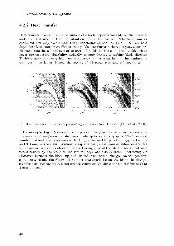
4 Turbomachinery Background
4.2.2 Heat Transfer
Heat transfer from a fluid to the surface of a body depends not only on the material
and fluid, but also on the flow situation around the surface. The heat transfer
coefficient can vary over a wide range depending on the flow field. The flow field
dependent heat transfer coefficient thus yields heat fluxes in the tip region, which are
different from those found over other parts of the blade. Hot spots are possible, which
lower the structural durability radically or may destroy a turbine blade directly.Turbines operate at very high temperatures, the first stage behind the combustion
chamber in particular. Hence, the cooling of this stage is of special importance.
Fig. 4.5: Sheerwood number representing amount of heat transfer (Cho et al., 2000).
For example, Fig. 4.5 shows contour plots of the Sherwood number, representingthe amount of heat/mass transfer, on a blade tip for various tip gaps. The Sherwood
number without gap is shown on the left, in the middle panel the gap is 1.5 mm
and 3.0 mm on the right. Without a gap the heat/mass transfer enhancement due
to horse-shoe vortices is observed at the leading edge of the blade. Additional local
peaks caused by the wake at the trailing edge are also existent. Increasing the
clearance between the blade tip and shroud, fluid enters the gap on the pressure
side. As a result, the Sherwood number characteristics on the blade tip changes
significantly. For example, a hot spot is generated on the blade tip trailing edge at
3 mm tip gap.
40

5 Experimental Setup
5.1 Measurement Principle/Optical Arrangement
Fig. 5.1 shows the schematic setup of the optical components in the measuring
circuit of the system. A superluminescent diode (SLD, Superlum Diodes model
SLD56-HP2, 10 mW) emits low coherence light into a singlemode fiber. A fiber
optical isolator protects the sensitive light source from backreflections and guidesthe light to a polarization insensitive optical circulator. The circulator is used to
transfer the light through a singlemode optical fiber to the endoscopic front end
(EFE), where a collimator lens directs the light out of the fiber onto the passing
blade tips. From there a small fraction of the incident light is reflected back onto
the collimator lens and into the fiber towards the circulator, where it is deflected
into the interferometer part of the measurement system. A small fraction (~ 1 %) of
the light is also reflected off the two surfaces of the collimator lens, which provides
a spatial reference.
SLD isolator
-L>variable
delay
ofrom / to
EFE/turbine
Following the nomencla¬
ture of Fig. 5.2, the light re¬
flected from the blade tips
is denoted as ray 1, the
light reflected from the lens
front and back surfaces as
rays 2 and 3 and the lightfrom the fiber end as rays
F, respectively. The lightbackreflected from the tur¬
bine blades and the front
end (rays F, 1, 2, 3) is
fed into two interferome¬
ter arms by a beam split¬ter. In the reference arm,
an acousto-optic modula¬
tor (AOM, NEOS model
26055) shifts the frequencyof the light by 55 MHz, cor¬
responding to several peri¬
ods within the blade pas¬
sage time (~ 10 ßs). The
delay arm contains a mo¬
torized variable delay line (VDL, General Photonics VariDelay). The light from
the two interferometer arms is recombined by another beam splitter/combiner and
a broadband photoreceiver (New Focus model 1811) serves as detector.
Ù
beam
splitter
acusto
opticmodulator
beam
combiner
photodiode
Fig. 5.
data processing with DSO and PC
1 Schematic setup of the optical parts for the
tip clearance probe.
41

5 Experimental Setup
-+t+- -H-+-
reflection at fiber end
-1-4%
dT=d na,r(T)
1 -
blade
lens
Fig. 5.2 Interaction between laser beam, front end and blade tip.
As shown in Fig. 5.2, the path length of ray 1 is longer than that of rays 2 and 3
or even ray F. Denote the tip clearance as dj-, the optical thickness of the collimator
lens as dj,, the distance between fiber end and lens as do and the path lengths of
both interferometer arms (between the two beam splitters/combiners) as lr and l^,
respectively. If the VDL is set such that lr + 2(d^ + di, + do) = Id, for example, the
part of ray 1 going through the reference arm interferes with those parts of ray F
which go through the delay arm. The frequency of the AOM is now recorded as a
beat signal at the detector, which can be detected as a peak in the power spectrum.
Similarly, interference between ray 3 and ray F is observed, when lr+2(djJ+do) = Id-This represents the lens back surface, whose position within the turbine is known.
In addition, by checking the delay setting where ray 2 and ray F interfere, i.e., when
lr + 2do = Id, the EFE can be monitored for failures.
5.2 Optical Frontend
As mentioned the sensitive optical parts and electronics are included in a separate
self-contained unit, placed sufficiently far away from the turbine. Only a singlemodefiber is needed to connect the interferometer part with the sensor front end, posi¬
tioned within the turbine casing. The length of this connecting fiber is arbitrary.For the test described in this thesis it was measuring approximately 20 meter.
The two meter long fiber optical sensor front end (Fig. 5.3) was custom-made bythe company "Fiber-Optic" in Spreitenbach, Switzerland. Its maximum operating
temperature is about 1000 K. Besides a standard fiber connector it consists of a
gold coated singlemode fiber. The fiber is placed within a flexible steel wire sleeve.
Within this sleeve the fiber is free to move, such to avoid stresses due to different
thermal expansions. At the front end's upper side is an approx. 1 cm thick and
30 cm long bent tube with a built-in fiber connector (a part of this tube is also
flexible). The tube consists also of a Swagelok connector for the installation within
the turbine casing. At the lower side of the front end a focusing sapphire lens,
approx. 1 5 mm in diameter, is embedded. The lens and a part of the fiber end are
bonded and permanently crimped together with the surrounding metal jacket. The
placements of fiber and lens are as described in Fig. 5.2.
42
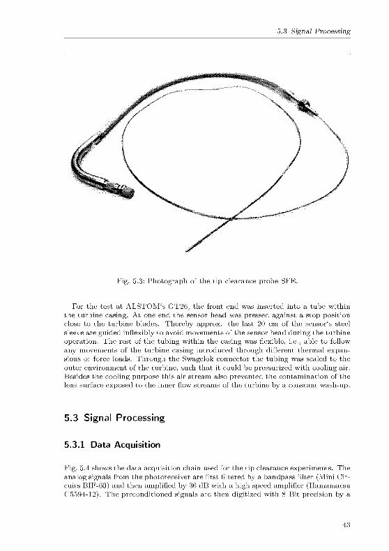
5.3 Signal Processing
Fig. 5.3 Photograph of the tip clearance probe SFE.
For the test at ALSTOM's GT26, the front end was inserted into a tube within
the turbine casing. At one end the sensor head was pressed against a stop position
close to the turbine blades. Thereby approx. the last 20 cm of the sensor's steel
sleeve are guided inflexibly to avoid movements of the sensor head during the turbine
operation. The rest of the tubing within the casing was flexible, i.e., able to follow
any movements of the turbine casing introduced through different thermal expan¬
sions or force loads. Through the Swagelok connector the tubing was sealed to the
outer environment of the turbine, such that it could be pressurized with cooling air.
Besides the cooling purpose this air stream also prevented the contamination of the
lens surface exposed to the inner flow streams of the turbine by a constant wash-up.
5.3 Signal Processing
5.3.1 Data Acquisition
Fig. 5.4 shows the data acquisition chain used for the tip clearance experiments. The
analog signals from the photoreceiver are first filtered by a bandpass filter (Mini Cir¬
cuits BIF-60) and then amplified by 36 dB with a high speed amplifier (HamamatsuC5594-12). The preconditioned signals are then digitized with 8 Bit precision by a
43

5 Experimental Setup
Digital Storage Oscilloscope - DSO (LeCroy LT347L). Data is then transferred to a
PC through a 10 MBit Ethernet connection for further analysis and storage. The
sampling rate and the acquisition window length are set through the DSO. The DAQis initiated by triggering the DSO with an external key-phaser of the test facility.
photo-receiver
signal
window length,
sampling rate
Fig. 5.4 Data acquisition - tip clearance probe.
5.3.2 Data Analysis
Two LabView (Ver. 7.1, National Instruments) programs perform the data storageand analysis. While one of them only stores the raw data for later analysis, the
second extracts tip clearances either on-line or from previously stored data sets.
During the critical gas turbine tests, data was initially stored. The raw data is first
bandpass filtered with a second-order Butterworth IIR-filter at a frequency range of
55 ± 1 MHz. A reliable indicator of a blade passage at the current delay line setting
was found to be the product of the signal variance and the maximum of the power
spectrum within a few microseconds sliding window. Either one of these factors
on its own did not yield a satisfactory discrimination between blade passages and
noise, especially at low signal levels. This product will be referred as beat signal
intensity for the remainder of this part of the thesis. Suppose that data is acquiredfor the entire duration of a turbine revolution. The VDL delay is varied in steps
after each acquisition and a new full-revolution trace is acquired. The step size for
the VDL has to be less than the coherence length of the light source. This, combined
with the given rotation rate of the turbine and the desired measurement range, is
an upper bound for the detection rate of the technique. A full scan over 1 mm in
steps of 40 /im on a turbine operating at 50 Hz thus requires at least 1 second. Note
that data acquisition and moving the VDL occurs during alternating revolutions. In
practice, achievable data transfer rates and the response time of the VDL motor led
to increased scan times.
Two approaches to reduce the amount of raw data were used. One is undersam-
phng of the DSO at sampling rates of 50, 20 and 10 MHz. The Butterworth filter
then had a frequency range of 5 ± 1 MHz. Noise from multiple frequency ranges
is convolved into the relevant frequency range.This leads to reduced signal-to-noiseratios (SNR). For tests in turbines, however, it was found to be practical. A further
reduction of the amount of data can be realized by only acquiring data within short
windows around the expected blade passage time. For turbine stages with many
blades and using window sizes which capture the blade passage reliably, however,
44
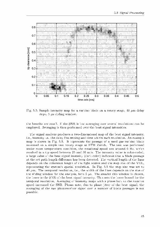
5.3 Signal Processing
time axis [ms]
Fig. 5.5: Sample intensity map for a turbine blade on a rotary stage, 40 /im delay
steps, 5 ßs sliding window.
the benefits are small. If the SNR is low averaging over several revolutions can be
employed. Averaging is then performed over the beat signal intensities.
The signal analysis produces a two-dimensional map of the beat signal intensity,
i.e., intensity vs. the delay line setting and time within each revolution. An example
map is shown in Fig. 5.5. It represents the passage of a used gas turbine blade
mounted on a simple test rotary stage at ETH Zurich. The test was performedunder room temperature condition, the rotational speed was around 6 Hz, which
resulted in a tip speed between 25 and 30 m/s. The intensity value is color-coded,
a large value of the beat signal intensity (dark color) indicates that a blade passage
at the set path length difference has been detected. The vertical length of the lines
depends on the coherence length of the light source and the step size of the VDL,
representing the system's spatial resolution. In Fig. 5.5 the step size was set to
40 /im. The temporal resolution, i.e., the width of the lines depends on the size of
the sliding window for the analysis, here 5 ßs. The smaller this window is chosen,the lower is the SNR of the beat signal intensity. This sets the lower bound for the
temporal resolution. Averaging of intensity maps with a phase-lock to the rotation
speed increased the SNR. Please note, due to phase jitter of the beat signal, the
averaging of the raw photoreceiver signal over a number of blade passages is not
possible.
45

5 Experimental Setup
46

6 Experiments
6.1 System Performance
6.2 LISA Turbine Tests
LISA, Fig. 6.1, is a research turbine test facility of the Laboratory of Turbomachin¬
ery at ETH Zurich. The important design features are mechanical precision, full
accessibility for instrumentation as well as quick assembly. The core of the test rigis an axial turbine with vertical orientation. The maximum power of 400 kW is
taken from a quasi atmospheric air circuit driven by a 750 kW radial compressor.
The turbine's power output is connected via an angular gear box to a generatorwith electrical power feedback. The air circuit consists of a cooler, which controls
the inlet temperature, a flow conditioning segment and a calibrated venturi-nozzle
integrated into the back flow pipe (Pfau, 2003). The results of LISA tip clearance
tests presented in this thesis were performed as a secondary application during tip
gap flow field manipulations (Behr et al., 2006).
Generator gjzlSafety Coupling 1
Venturi Nozzle
Bypass System
Safety Coupling 2
Flow ConditioningStretch
Compressor
Fig. 6.1: Schematic view of LISA axial test turbine (Pfau, 2003).
47

6 Experiments
1 H
5 10 15 20 25 30 35 40 45
time after key-phaser [ms]
50
3 4 5 6 7
time after key-phaser [ms]
10
Fig. 6.2: Tip clearance distribution of LISA rotor, intensity map
The full view suggests that not all blades were detected. The detail view in the lower panel,
however, shows that this is just an artifact of the visualization routine.
48

6.2 LISA Turbine Tests
Due to the high mechanical precision of the turbine as well as the use of cold
gas (approx. 50° C) and therefore small thermal expansion responses, the primary
objective of the measurements was to scan with high spatial resolution, i.e., small
interferometer delay steps. Fig. 6.2 shows a two-dimensional beat signal intensity
map of 50 milliseconds at a rotation speed of 2700 rpm, i.e., spanning two full
revolutions. The sampling rate was set to 50 MHz, the step size to 20 /im. The
complete scan over 0 3 mm lasted 60 seconds. The rotor with a tip diameter of
798 6 mm [±0 01 mm] consists of 54 blades machined into one single aluminum ring
by electrical erosion. The smooth aluminum surface of the blade tips yields a highbackreflection level. Together with the signal amplification due to the interference
with the reference reflection in the EFE, the SNR in these tests is not critical. The
rotor blade tips show a sinusoidal clearance behavior with an amplitude of approx.
50 (im. This value might be due to a small eccentricity of the rotor assembly within
the turbine.
16 17
day-time [hh]
Fig. 6.3 LISA tip clearance behavior over operation time.
In Fig. 6.3 the average, the maximum and the minimum tip clearance of the 54
blades was recorded over time. The sampling rate was set 10 MHz and the step size
to 20 /im. In this test, a separate spatial reference was provided by a window which
was placed approximately flush with the casing. The scan range was increased to
1 15 mm such to include this reference location as well. A scan then lasted 95 seconds.
The long-term clearance behavior of the turbine shows a small decrease of the gap byabout 100 /im (before 13 hours daytime, the turbine was rotating at a lower speed).In addition a smooth increase and decrease of the tip clearance can be detected.
This might be due to a slow gradual rotation of 20° of the turbine casing during the
simultaneously performed flow field measurements.
49
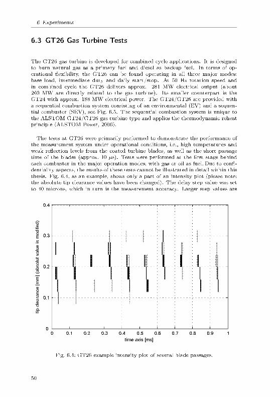
6 Experiments
6.3 GT26 Gas Turbine Tests
The GT26 gas turbine is developed for combined cycle applications. It is designedto burn natural gas as a primary fuel and diesel as backup fuel. In terms of op¬
erational flexibility, the GT26 can be found operating in all three major modes:
base load, intermediate duty and daily start/stop. At 50 Hz rotation speed and
in combined cycle the GT26 delivers approx. 281 MW electrical output (about260 MW are directly related to the gas turbine). Its smaller counterpart is the
GT24 with approx. 188 MW electrical power. The GT24/GT26 are provided with
a sequential combustion system consisting of an environmental (EV) and a sequen¬
tial combustor (SEV), see Fig. 6.5. The sequential combustion system is unique to
the ALSTOM GT24/GT26 gas turbine type and applies the thermodynamic reheat
principle (ALSTOM Power, 2006).
The tests at GT26 were primarily performed to demonstrate the performance of
the measurement system under operational conditions, i.e., high temperatures and
weak reflection levels from the coated turbine blades, as well as the short passage
time of the blades (approx. 10 ßs). Tests were performed at the first stage behind
each combustor in the major operation modes, with gas or oil as fuel. Due to confi¬
dentiality aspects, the results of these tests cannot be illustrated in detail within this
thesis. Fig. 6.4, as an example, shows only a part of an intensity plot (please note:
the absolute tip clearance values have been changed). The delay step value was set
to 40 microns, which in turn is the measurement accuracy. Larger step values are
iNllI0 0.1 0.2 0.3 0.4 0.5 0.6 0.7 0.8 0.9 1
time axis [ms]
Fig. 6.4: GT26 example intensity plot of several blade passages.
50

6.3 GT26 Gas Turbine Tests
EV-Cobustor EV-Burner
Fig. 6.5: GT26 schematic illustration.
not possible, due to the coherence length of the light source of approx. 50 /im. The
time axis is resolved with 5 microseconds. The signatures show that the blade tip is
not flat, but slightly beveled.
In general it can be said that even under real gas turbine conditions, the sensor
still works well. However in terms of measurement system performance a few issues
need to be addressed. The EFE with its optical parts close to the hot gas flow showed
no irreversible failures. The high temperatures and the mechanical loads due to the
casing movements during its warm-up did not damage the optics. The 20 m fiber
optical extension cable also withstood the temperatures within the turbine enclosure,which can reach up to approx. 80°C close to the turbine. The SNR was high enoughto operate with a sampling rate of 50 MHz and without averaging. During the start¬
up of the turbine, i.e., the first 30 minutes after ignition, the SNR was comparativelylow and just above the sensing limit. Furthermore, after 5 hours of operation under
base-load conditions, the SNR dropped over a period of 20-30 minutes. Finally and
reproducibly in two tests at around 5-6 hours of operation, the SNR was too low to
detect any tip clearances.
Both phenomena are probably caused by changes in the thermal behavior of the
optical fiber within the casing and the turbine enclosure. The first decrease of the
SNR at the start-up might be due to the fast temperature rise and therefore the
huge thermal stresses at the EFE. After 30 minutes, the rate of the temperature rise
is decreased. The whole EFE is heated-up and due to its design the fiber within
the EFE experiences no mechanical stresses. The second decrease can be attributed
to the relatively small thermal load in the turbine enclosure. The extension cable
was protected by a thick PVC tube (standard telecom cable). Its thermal insulation
might cause the long response time to the temperatures in the enclosure building.The assembly of the fiber and the PVC is not specifically designed to balance me¬
chanical stresses of the fiber at higher temperatures. Thus, under stress the fiber
51

6 Experiments
transmissivity can drop by orders of magnitude. However, both assumptions have
to be investigated in further tests.
During the GT26 tests the beat signal frequency was shifted by 10 to 15 MHz.
This is due to Doppler shift in the backrefiected light from the blade tips. If the
surface of the blade tips moves not perpendicular to the sensor head, a Dopplershift can be detected as in reference beam LDA applications, see Chapt. 3.2.2. Anyrelative velocities parallel to the beam axis between the reference reflection and the
blade reflection will result in a Doppler signal. In the GT26 the blade tips are
relatively rough, plus they are slightly beveled. The roughness leads to a spectral
broadening of the beat signal frequency of up to ± 2 MHz. The bevel of the tip
causes a general frequency shift. It might also be possible that the sensor was
mounted at a small angle. Taking into account the circumferential velocities at the
GT26 of approx. 350 m/s, the observed frequency shift corresponds to an angle of
about 1-2° off the normal direction.
In the data acquisition and analysis this Doppler shift has to be considered. All
bandpass filter devices have to match the shifted frequency. For industrial applica¬tions such uncertainties in the analysis regime should be avoided.
52
7 Conclusions / Outlook
Proof-of-principle measurements were presented for a novel tip clearance measure¬
ment technique with high spatial and temporal resolution. Independent of the dis¬
tance between the output coupler lens and the blade tip the absolute spatial accuracy
is within 50 microns. Variations in fluid or material temperatures have no influence
other than minimal changes in the refractive index. Data acquisition rates for tip
clearance profiles on the order of seconds allows monitoring of transient effects duringturbine start-up and shut-down. Simultaneously with the tip clearance, the blade
passage times are measured, facilitating the detection of blade oscillations.
The tests at the LISA turbine test facility and the GT26 gas turbine under oper¬
ating conditions already led to qualified results. For the first time the tip clearance
behavior from the first stage of a large scale gas turbine cold be monitored for differ¬
ent engine loads. However, for a second prototype the aspects of industrial operation
have to be considered. One focus is the thermal behavior of the optical fibers close
to the turbine. In particular the problem in long-term tests has to be solved. The
exposure of the optical connection cable to an environment of 80° C leads to a re¬
versible failure after approx. 5 hours. With special assemblies the optical fiber in
the covering tube can be guided stress-free, which should solve this problem.
The second focus for further developments lies in the observed Doppler shifts,which lead to a shift of the beat signal. On one hand, with this the acousto-optic
modulator with its fixed frequency shift is unnecessary. On the other hand, depend¬
ing on the mounting orientation of the sensor to the blade tip surface and blade tip
velocity, the Doppler shift will have different values. For this reason, a flexible de¬
modulation of the signal into a fixed frequency band might be one possible technical
solution. This is particularly important in a situation where one signal processing
unit operates with more than one sensor front end, which is an additional possible
improvement for the system. Therefore, tests with amplitude modulated SLD and
a following frequency lock-in have been made with promising results.
With the use of an optical multiplexer measurements with a series of sensor front
ends mounted around the circumference of the turbine casing are possible. Still
only one light source and one signal processing unit are necessary. The multiplexer
just needs to be inserted between the circulator and the front ends. Then the tip
clearance for each sensor position can be measured successively. The increase in the
measurement time for this scenario is minimal, since it should be possible to switch
between two sensor front ends within one or two turbine revolutions.
53

7 Conclusions / Outlook
54

Part III
Self-Referencing Velocimetry
55

Introduction and Motivation
Velocimetry techniques for boundary layer measurements face two challenges spatialresolution and non-intrusiveness. In most technical applications, the thickness of the
boundary layers is on the order of millimeters such that sub-millimeter resolution
is required for meaningful measurements. The requirements are even higher when
the viscous sub-layer and the log-layer have to be resolved (Schhchting & Gersten,
2000).
Traditionally, hot-wire anemometry (or constant temperature anemometry, CTA,as well as constant current anemometry) has been the method of choice for such
measurements, e.g., (Haggmark et al., 2000, Ligrani & Bradshaw, 1987, Wolff et al.,
2000). The typical diameter of the wire is on the order of micrometers. They are
typically 1-2 mm long, but the spatial resolution in the wall-parallel direction is not
critical. Because the measurement location is identical to the probe location, the
probe has to be moved to obtain the velocity profile across the boundary layer. This
makes this technique problematic for measurements over moving objects. But even
over stationary surfaces, the thermal conductivity of the wall leads to systematic
errors of the measured velocity (Durst & Zanoun, 2002, Durst et al., 2001).
Recently, micro-PIV has been applied to high-resolution boundary layer measure¬
ments. PIV either requires optical access from at least two directions (one for the
illuminating laser sheet, the second for the camera) or a depth resolving focusing
optic as in microscopy (Lin & Perhn, 1998, Meinhart et al., 2000). Depending on
the geometry and the object's movement, this might not be feasible. Laser-Doppler
velocimetry (LDV) lacks the required spatial resolution, which is determined by the
diameter of the intersecting laser beams and the crossing angle. LDV measures the
velocity component perpendicular to the long axis of the intersection ellipsoid. This
means that the spatial resolution is poorest in the direction where it is most critical.
With a novel technique using a tilted fringe system, the LDV intersection volume can
also be resolved in the order of microns (Buttner & Czarske, 2001, 2003). Distributed
laser Doppler velocimetry (DLDV) (Gusmeroh & Martinelli, 1991), a reference beam
LDV using low coherence light, defines the measurement location as the focal region.
The low coherence interferometry then allows further resolution within the focal re¬
gion. In this respect, the technique shares many aspects with optical coherence
tomography (OCT) (Tomlins & Wank, 2005). DLDV can be seen as a very similar
technique to the approach described in this thesis.
In a PIV image, the flow is visible together with the object such that it is possibleto deduce the measurement location (relative to the surface) from the data without
independent knowledge of the object's trajectory. Nevertheless, as mentioned, the
PIV installation itself might be very challenging. CTA, LDV and DLDV on the
other hand have all in common, that they are not self-referencing. At any instance,
the relative location of the object to the measurement volume has to be known. If
57
the motion is irregular or if the shape of the object changes over time, this might
pose a problem.
The new technique is self-referencing with respect to its vertical measurement
location to an arbitrary surface and has a spatial resolution only depending on the
coherence length of the light source (e.g., see interferogram Fig. 2.3). It measures
in-plane and out-of-plane components of the velocity vector. The sensitivity to out-
of-plane velocities (which are normally much lower) is tenfold (value can be adjusted)higher than for in-plane velocities. As for LDV and PIV, particle seeding is required.
Conceptually, planar measurements (cf. PIV) are also possible with self-referencing
capabilities.
The working principle of this new technique is explained using the example of a
two-component boundary layer profiler based on the Doppler effect. The systems
is spatially self-referenced relative to a surface, but applications where the sensor
head is the reference follow the same principle. For the new approach a notation is
introduced with "SR" standing for self-referencing, i.e., SR-LDV.
58

8 Self-Referencing Low Coherence
Velocimeter
8.1 Basic Working Concept
The new technique combines flow velocimetry measurements with self-referencing
qualities by the use of low coherence interferometry. The measurement location is
selected based on its distance from an object. This object can either be the sen¬
sor head itself or an external surface, which might be moving relative to the sensor
head. The distance can be adjusted without moving optical parts in the sensor
head, simply by varying the path lengths in the interferometer arms. Irrespectiveof any movement of the surface, measurements are always performed at a set dis¬
tance from the wall. One could say that the measurement location is in wall-fixed
coordinates instead of lab-fixed coordinates as for other techniques. The absolute
accuracy of the measurement location and the spatial resolution is on the order of
tens of micrometers, depending on the properties of the low coherence light source.
This technical approach is applicable to single-beam single-component measure¬
ments, as well as to multi-beam multi-component measurements (cf. Laser-Doppler
Velocimetry - LDV or Laser-Two-Focus Velocimetry - L2F). In the future, with a
probable rise of power of broadband light sources, two-dimensional measurements
(cf. Particle Imaging Velocimetry PIV) might also be possible with self-referencing
image planes or a pointwise scanning technique. As mentioned similar to most other
optical velocimetry techniques, flow seeding is required.
This chapter outlines the principles of the self-referencing technique for LDV and
L2F applications. The new self-referencing aspect will be indicated with the prefix
SR, i.e., writing SR-LDV or SR-L2F.
8.2 Self-Referencing Laser-Doppler Velocimetry (SR-LDV)
8.2.1 Measurement Principle - SR-LDV
The system consists of two main parts the interferometer unit and the sensor head.
Fig. 8.1 shows the schematic setup of the optical components in the interferometer
unit of the system. A superluminescent diode (SLD, Superlum Diodes model SLD56-
HP2, 1310 nm, 10 mW) emits low coherence light into a singlemode fiber. The dotted
line in Fig. 2.3 is the autocorrelation function of the SLD. The coherence length is
represented as the FMHW of the peak (~ 35 /im). A fiber optical isolator protects
59
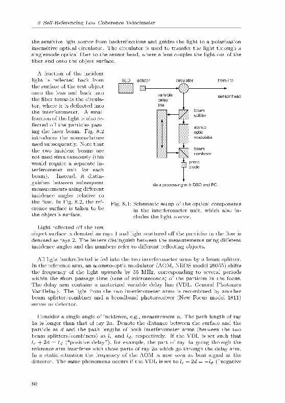
8 Self-Referencing Low Coherence Velocimeter
the sensitive light source from backreflections and guides the light to a polarizationinsensitive optical circulator. The circulator is used to transfer the light through a
singlemode optical fiber to the sensor head, where a lens couples the light out of the
fiber and onto the object surface.
A fraction of the incident
light is reflected back from
the surface of the test objectonto the lens and back into
the fiber towards the circula¬
tor, where it is deflected into
the interferometer. A small
fraction of the light is also re¬
flected off the particles pass¬
ing the laser beam. Fig. 8.2
introduces the nomenclature
used subsequently. Note that
the two incident beams are
not used simultaneously (thiswould require a separate in¬
terferometer unit for each
beam). Instead, it distin¬
guishes between subsequentmeasurements using different
incidence angles relative to
the flow. In Fig. 8.2, the ref¬
erence surface is taken to be
the object's surface.
Light reflected off the test
object surface is denoted as rays 1 and light scattered off the particles in the flow is
denoted as rays 2. The letters distinguish between the measurements using different
incidence angles and the numbers refer to different reflecting objects.
All light backrefiected is fed into the two interferometer arms by a beam splitter.In the reference arm, an acousto-optic modulator (AOM, NEOS model 26055) shifts
the frequency of the light upwards by 55 MHz, corresponding to several periodswithin the short passage time (tens of microseconds) of the particles in the focus.
The delay arm contains a motorized variable delay line (VDL, General Photonics
VariDelay). The light from the two interferometer arms is recombined by another
beam splitter/combiner and a broadband photoreceiver (New Focus model 1811)serves as detector.
Consider a single angle of incidence, e.g., measurement a. The path length of ray
la is longer than that of ray 2a. Denote the distance between the surface and the
particle as d and the path lengths of both interferometer arms (between the two
beam splitters/combiners) as lr and Id, respectively. If the VDL is set such that
lr + 2d = Id ("positive delay"), for example, the part of ray la going through the
reference arm interferes with those parts of ray 2a which go through the delay arm.
In a static situation the frequency of the AOM is now seen as beat signal at the
detector. The same phenomena occurs if the VDL is set to lr — 2d = —l^ ("negative
SLD isolator
—Q- ovariable
delayline
/, i l
l\
\
5
beam
splitter
acusto
opticmodulator
beam
combiner
photodiode
data processing with DSO and PC
Fig. 8.1 Schematic setup of the optical components
in the interferometer unit, which also in¬
cludes the light source.
60
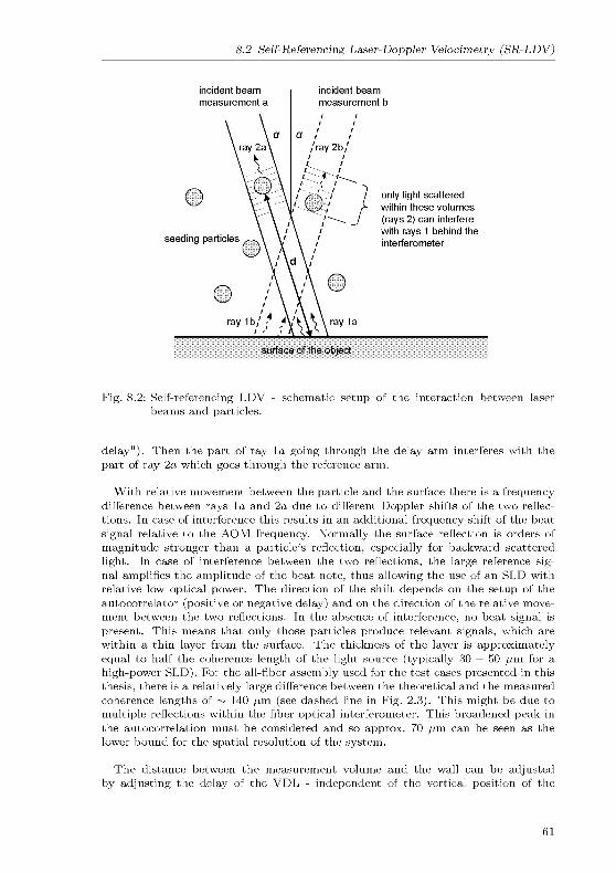
8.2 Self-Referencing Laser-Doppler Velocimetry (SR-LDV)
incident beam
measurement a
incident beam
measurement b
only light scattered
within these volumes
(rays 2) can interfere
with rays 1 behind the
interferometer
surface of the object
Fig. 8.2: Self-referencing LDV
beams and particles.
schematic setup of the interaction between laser
delay"). Then the part of ray la going through the delay arm interferes with the
part of ray 2a which goes through the reference arm.
With relative movement between the particle and the surface there is a frequencydifference between rays la and 2a due to different Doppler shifts of the two reflec¬
tions. In case of interference this results in an additional frequency shift of the beat
signal relative to the AOM frequency. Normally the surface reflection is orders of
magnitude stronger than a particle's reflection, especially for backward scattered
light. In case of interference between the two reflections, the large reference sig¬nal amplifies the amplitude of the beat note, thus allowing the use of an SLD with
relative low optical power. The direction of the shift depends on the setup of the
autocorrelator (positive or negative delay) and on the direction of the relative move¬
ment between the two reflections. In the absence of interference, no beat signal is
present. This means that only those particles produce relevant signals, which are
within a thin layer from the surface. The thickness of the layer is approximately
equal to half the coherence length of the light source (typically 30 — 50 /im for a
high-power SLD). For the all-fiber assembly used for the test cases presented in this
thesis, there is a relatively large difference between the theoretical and the measured
coherence lengths of ~ 140 /im (see dashed line in Fig. 2.3). This might be due to
multiple reflections within the fiber optical interferometer. This broadened peak in
the autocorrelation must be considered and so approx. 70 /im can be seen as the
lower bound for the spatial resolution of the system.
The distance between the measurement volume and the wall can be adjusted
by adjusting the delay of the VDL - independent of the vertical position of the
61

8 Self-Referencing Low Coherence Velocimeter
sensor head. Irrespective of any movement of the surface, measurements are always
performed at a set distance from the wall. One could say that the measurement
location is in wall-fixed coordinates instead of lab-fixed coordinates as for other
techniques.
Each measurement yields the relative velocity between reference surface and par¬
ticle in the direction of the laser beam. In order to determine the wall-normal and
wall-parallel velocity components separately, a second measurement with a different
incidence angle is required. This is shown in Fig. 8.2 as measurement beam b. These
two measurement do not need to be taken simultaneously and the measurement vol¬
umes of the two beams do not necessarily coincide exactly. In fact, their offset will
typically vary along the wall-normal direction. Consequently, the beams do not look
at the same horizontal position. But the spacing of the beams and their diameter
is small and since the resolution in wall-parallel direction is usually not crucial, this
should not pose a problem.
Throughout this thesis the laser beams a and b will be indicated with either for¬
ward (looking in the upstream direction) or backward (looking in the downstream
direction).
8.2.2 Data Analysis - SR-LDV
Consider the velocity vector u = (u,v), where u is the wall-parallel velocity and v is
the wall-normal component. Assume (without loss of generality) that the bisector of
the laser beams from measurements a and b is perpendicular to the wall (as shown
in Fig. 8.2). Interference between rays la and 2a produces a peak in the power
spectrum at
2
fa = —(v cosa + u svaa) + fAOM (8.1)A
(A is the wavelength of the laser beams). The Doppler shift between rays 16 and 26
(from a second measurement) occurs with the opposite sign for the u component.
The peak is thus at
2
fb = —(v cosa - u svaa) + fAOM (8.2)A
Denote the spacing of the two peaks as AF = \fa — fb\ and the average Dopplershift as Y2 F =
g {fa + fb) — fAOM- The velocity vector is then obtained from
AAF ASF, N
u = and v = (8.3)Asina 2cosa
Since a is small, the sensitivity to wall-normal velocities (dYlF/dv) is much largerthan to in-plane velocities (dAF/du). The ratio of the sensitivities is 1 /tana. This is
desirable, because the wall-normal velocities are much smaller than the wall-parallelvelocities in boundary layer types of flows.
62

8.3 Self-Referencing Laser-Two-Focus Velocimetry (SR-L2F)
In order to relate the sign of the shift of the beat signal, / — fAOM, to the flow
direction, one has to account for the setting and for the design of the interferometer.
With an interferometer design as shown in Fig. 8.1, consider a case where the lightreflected off the particle is more blue shifted, i.e., f2 > f\ (where f\ and f2 are
the frequencies of rays 1 and 2, respectively, as shown in Fig. 8.1). When the
interferometer is set such that the path lengths match when ray 2 passes throughthe AOM and ray 1 passes through the delay arm, i.e., to a negative delay, the beat
note will have the frequency (Jaom + fl) — f\- When, on the other hand, ray 2
passes through the delay arm and ray 1 is frequency shifted, the beat note will have
the frequency (Jaom + /l) — Ï2- For both scenarios the shift of the beat signalhas opposite signs. The same case with an interferometer design where the AOM is
included in the delay arm, will lead to beat signal shifts in the opposite direction.
It has been assumed that the orientation of the sensor head to the surface is known.
Lacking the orientation of the wall relative to the detector the flow direction relative
to the wall cannot be obtained. In this case only the flow velocity components
along directions aligned in relation to the sensor head can be determined. Another
assumption was that the wall is stationary. When the wall moves relative to the
sensor head, the measured velocities are relative to the wall speed.
8.3 Self-Referencing Laser-Two-Focus Velocimetry (SR-L2F)
8.3.1 Measurement Principle - SR-L2F
The key features of this technique are the same as for SR-LDV, namely low coherence
velocimetry with spatial self-referencing capability. Now, however, two laser beams
are used to measure a single velocity component. The standard laser-two-focus
principle is based on the measurement of the time of flight of a particle between two
light gates. The light gates are formed by two highly focused laser beams, which
allow the detection of relatively small particles. The lengths of the focal regions
are usually still several hundred micrometers, which limits the spatial resolution in
the beam-wise direction. Also, the absolute location of the focal region relative to
an object is not known, only the relative distance to the focusing optic. Using low
coherence light and an interferometer setup resolves both limitations. Only particles,which pass at a certain distance from the wall across the focal region produce a beat
signal.
The changes to the SR-LDV experimental setup are twofold first, the three-port
polarization independent circulator is replaced by a four-port polarization dependentcirculator. It provides two independent beams of perpendicular polarization. The
incoming light from these two ports is directed into the interferometer.
Furthermore, in the SR-L2F setup both laser beams are set perpendicular to
the surface. Therefore, no Doppler shift is generated by wall-parallel velocities.
The extraction of velocity data follows the common L2F analysis techniques (seeChapt. 3.3), except that it derives the data from the beat signals. The measured
velocities are then relative to the sensor head. In addition, the system is sensitive
to out-of-plane velocities by detecting the Doppler shift, as in SR-LDV.
63
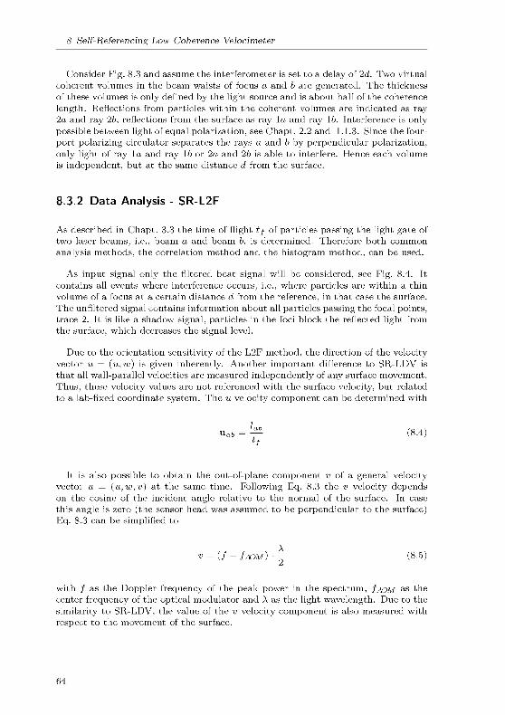
8 Self-Referencing Low Coherence Velocimeter
Consider Fig. 8.3 and assume the interferometer is set to a delay of 2d. Two virtual
coherent volumes in the beam waists of focus a and 6 are generated. The thickness
of these volumes is only defined by the light source and is about half of the coherence
length. Reflections from particles within the coherent volumes are indicated as ray
2a and ray 26, reflections from the surface as ray la and ray 16. Interference is only
possible between light of equal polarization, see Chapt. 2.2 and 1.1.3. Since the four-
port polarizing circulator separates the rays a and 6 by perpendicular polarization,
only light of ray la and ray 16 or 2a and 26 is able to interfere. Hence each volume
is independent, but at the same distance d from the surface.
8.3.2 Data Analysis - SR-L2F
As described in Chapt. 3.3 the time of flight tf of particles passing the light gate of
two laser beams, i.e., beam a and beam 6, is determined. Therefore both common
analysis methods, the correlation method and the histogram method, can be used.
As input signal only the filtered beat signal will be considered, see Fig. 8.4. It
contains all events where interference occurs, i.e., where particles are within a thin
volume of a focus at a certain distance d from the reference, in that case the surface.
The unfiltered signal contains information about all particles passing the focal points,
trace 2. It is like a shadow signal, particles in the foci block the reflected light from
the surface, which decreases the signal level.
Due to the orientation sensitivity of the L2F method, the direction of the velocityvector u = (u,w) is given inherently. Another important difference to SR-LDV is
that all wall-parallel velocities are measured independently of any surface movement.
Thus, these velocity values are not referenced with the surface velocity, but related
to a lab-fixed coordinate system. The u velocity component can be determined with
Uab = ^ (8.4)
It is also possible to obtain the out-of-plane component v of a general velocityvector u = (u,w,v) at the same time. Following Eq. 8.3 the v velocity depends
on the cosine of the incident angle relative to the normal of the surface. In case
this angle is zero (the sensor head was assumed to be perpendicular to the surface)Eq. 8.3 can be simplified to
v = (f- fAOM) • - (8.5)
with / as the Doppler frequency of the peak power in the spectrum, fAOM as the
center frequency of the optical modulator and A as the light wavelength. Due to the
similarity to SR-LDV, the value of the v velocity component is also measured with
respect to the movement of the surface.
64
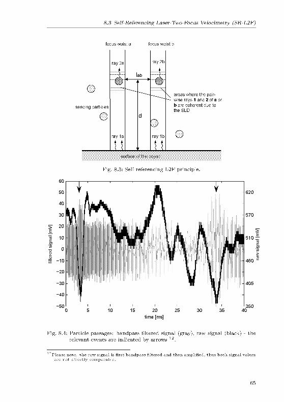
8.3 Self-Referencing Laser-Two-Focus Velocimetry (SR-L2F)
focus waist a focus waist b
o
seeding particles
o
ray 2a
ray 1a
i i
lab
ray 2b
\
3
ray 1b
i i
areas where the pair-
wise rays 1 and 2 of a or
b are coherent due to
the SLD
o
surface of the object
Fig. 8.3: Self-referencing L2F principle.
Fig. 8.4: Particle passages: bandpass filtered signal (gray), raw signal (black) - the
relevant events are indicated by arrows 12.
Please note: the raw signal is first bandpass filtered and then amplified, thus both signal values
are not directly comparable.
65

8 Self-Referencing Low Coherence Velocimeter
66

9 Experiments
9.1 Signal Processing
Fig. 9.1 shows the data acquisition chain for the velocimetry experiments. The analog
signals from the photoreceiver are first filtered by a bandpass filter (Mini Circuits
BBP-60) and then amplified by 36 dB with a high speed amplifier (HamamatsuC5594-12). The preconditioned signals are then digitized with 8 bit precision by a
photo-receiver
signal
window length,
sampling rate
Fig. 9.1 Data acquisition - boundary layer profiler.
Digital Storage Oscilloscope - DSO (LeCroy LT347L). The data is finally transferred
to a PC for further analysis and storage. The sampling rate and the acquisition
window length are set through the DSO. The data acquisition is triggered by a
particle passing the laser beam at the correct distance from the reference surface,
i.e., when the bandpass filtered signal exceeds a threshold (see also Fig. 8.4). The
dips in the unfiltered signal during relevant particle passages (indicated by arrows)were caused by a partial blockage of ray 1 through the particle. The subsequent data
analysis was performed by a LabView program (Ver. 7.1, National Instruments).
For the SR-LDV measurements, the raw data is first bandpass filtered with a
second-order Butterworth IIR-filter. Then the power spectrum of the signal is cal¬
culated with the standard LabView Fast-Fourier Transformation - FFT algorithm.
Next, from the power spectrum the frequency information of a particle passage is
extracted by the LabView peak detection routine. The threshold for the peak detec¬
tion is manually adjustable, as well as the number of points used to interpolate the
position of the frequency peak. Typical settings used during the experiments are 10
points for the interpolation routine and a threshold twice as high as the noise level.
Finally the frequency data is converted into velocity as described in Sect. 8.2.2.
In the L2F routine, after the bandpass filtering, the signal envelope is determined
by a Hubert transformation and another lowpass filtering step. Signals above a
certain threshold are then indicated with 1 and below the threshold with 0. Next,this binary signal is autocorrelated. In the autocorrelation function all peak positions
67

9 Experiments
are detected with the LabView peak-detection routine. Furthermore, the distribution
function of the time of flight data is determined with histogram method. Finally,with the knowledge of the light gate spacing, the time of flight is converted into
velocity data (see Sect. 8.3.2).
9.2 Measurements in Liquid Flows
9.2.1 Poiseuille Flow - Rectangular Channel
The tests in a closed rectangular channel were primary realized to demonstrate
the performance of the measurement system under controlled conditions. Also the
comparison to the theoretical profile should be established. In addition, the velocity
profile within the channel was measured in the SR-LDV and in the SR-L2F mode,
providing similar but in the way of the analysis routine independent data (frequencyvs. time of flight measurement).
The dimensions of the channel are 20 mm by 3.3 mm with a length of approx.
500 mm. Optical access was possible through the channel walls (Plexiglas, 1.5 mm
thick). In both measurement configurations the sensor head was placed approx.
6 cm above the channel and the diameter of the coupling lens was 5 millimeter.
At the back side of the lower Plexiglas wall a retro-reflecting foil was affixed (seeFig. 9.2). The orientation of the channel was horizontal. Oil (Bizol, CGPL-68) was
sucked through the channel at constant flow rates. As seeding aluminum powderwith particles sizes of approx. 50 microns was used.
optical access through the upper wa
Plexiglas walls
With the retro-reflector it was
possible to obtain good reflections,also at high incident angles (neededfor the SR-LDV measurements). In
that way the reference reflection
was not directly the channel bot¬
tom. Hence, the optical delay set
in the interferometer representing
the bottom of the channel is not
zero. The relative measurement
retro-reflecting foilpositions in the channel were recal¬
culated under the consideration of
the refractive index of the oil and
the mentioned offset.Fig. 9.2 Optical access - rectangular channel
experiment.
Fig. 9.3 shows the comparison of
the three flow profiles (parabolic theory, SR-LDV, SR-L2F). In the SR-LDV mea¬
surements the observation angle was ± 14°, indicated with either forward or back¬
ward. The optical delay in the autocorrelator (Chapt. 5, Fig. 5.1) was set to positive
values. Therefore, the observed beat signals are smaller than the AOM frequencyfor the forward setup and higher for the backward setup at positive flow directions.
The error bars for SR-LDV representing the minimum and maximum velocity out
of 30-50 measurements for each position. The standard deviation is with approx.
68

9.2 Measurements m Liquid Flows
Fig. 9.3 Poiseuille flow profile measured with SR-LDV and SR-L2F, Re œ 2.
0.5 mm/s (200 Hz) nearly constant over the profile. All data was obtained at a
sampling rate of 50 MHz and with a measurement window of 100 k samples. Thus,the resolution of the power spectrum in this test was 500 Hz. At the highest veloc¬
ity, a particle passage almost covered the acquisition window. Undersamphng shifted
the beat signal to 5 MHz. For the L2F measurement the plotted velocity at each
position is always related to maximum in the histogram of class occurrences of the
time of flight data. Both measurements compared with each other and compared to
the theoretical parabolic profile show a good agreement.
9.2.2 Couette Flow - Rotating Cylinder
The measurements between two coaxial rotating cylinders, i.e., Taylor-Couette flow,were performed to demonstrate the self-referencing capabilities. A metal cylinder
(outer diameter 2rz = 83 mm) was placed coaxially in the center of a Plexiglas
cylinder (inner diameter 2r0 = 89 3 mm, 5 mm thick). The length of both cylindersis approx. 30 cm, they were installed vertically. The resulting gap, of about 2 85 mm,
was filled with olive oil and aluminum powder (particle size m 50 /ai) as seeding.The inner cylinder could rotate with frequencies of up to Q/(27r) = 6 revolutions per
second.
The SR-LDV sensor head was located approx. 60 mm radially outside of the outer
cylinder and slightly tilted against the flow direction. Due to the beam deflections at
the curved Plexiglas surface, the angle of incidence relative to the inner cylinder is
69

9 Experiments
0 05 1 15 2 25 3 35 4
optical delay [mm]
Fig. 9.4 Measured velocity profile of Couette flow at 0.21 m/s surface speed.
not known a prion. It was later calculated to be approx. 15°, based on the measured
frequency shifts near the wall and the known rotation rate. For these flow param¬
eters the flow is laminar and the flow is parallel such that the wall-normal velocity
component is known to be zero. Measurements with a single incidence angle are
thus sufficient.
A retro-reflecting foil was attached to the inner cylinder (the reference surface).The primary reason for this was to increase the reflection level from the reference
surface back into the collimator lens. The reflections from the metal cylinder are
otherwise very directional and thus largely miss the collection lens for sufficiently
large angles of incidence. The light is not reflected from the surface of the foil, but
enters it and is reflected from the internal structures. It thus covers a small pathwithin it. This has the welcome side effect that the (optical) reference surface does
not coincide with the foil surface, but lies within the foil. This allows one to mea¬
sure closer to the reference surface. Normally, measurements at or near the reference
surface (within the first 50 to 100 /im) require that the path lengths through both
interferometer arms are nearly equal. In that case, however, all other reflections also
produce interference with themselves. This results in a high background level of the
beat signal, above which passing particles cannot be detected. The offset due to
the path length within the reflector foil was measured to be 0 18 mm. Owing to the
spatially periodic structure of the retro-reflector, the backreflection level is not con¬
stant, but instead highly modulated. It was also observed that, due to a shadowing
effect, the reflection level from the retro-reflector and walls decreases during particle
passages. However, in the bandpass filtered signal only the beat signals are visible.
70

9.2 Measurements m Liquid Flows
In Fig. 9.4 the frequency shift of the beat signal is plotted versus the optical delayof the interferometer. The surface velocity Us of the inner rotating cylinder was
0 21 m/s. In a coordinate system fixed with the rotating cylinder, the fluid flow
direction is negative, i.e., at the stationary outer Plexiglas wall the relative velocityis the highest and at the moving cylinder's surface it is zero, with a linear profilein-between. The error bars represent the minimum and maximum of the frequencyshifts out of 10 to 30 particle passages for each position. The standard deviation is
between 1 and 2 kHz and nearly constant across the gap. Data with high spatialresolution was obtained close to each surface and within three central regions. Close
to the fixed Plexiglas wall the data rate drops rapidly, because the absolute flow
speed is close to zero and the number of particle passing the laser beam per unit
time decreases. Note that the surface of the inner cylinder corresponds to an optical
delay of 0 18 mm, the optical path within the retro-reflector.
Fig. 9.5 shows the frequency shift of the beat signal versus the optical delay of
the interferometer at different rotation speeds of the cylinder. The data series are
labeled by the surface speed of the rotating cylinder and the corresponding Taylornumber (77 as the dynamic viscosity)
/— /\3/2
i/r.u (r0—
r.)'
,
Ta=VV
^ (9.1)V
The maximum rotation speed of this test setup was approx. 6 Hz, correspondingto a surface velocity of Us = 1 55 m/s. The data at all rotation speeds shows a
linear behavior in accordance with theory. Fig. 9.6 shows the range of the measured
0 05 1 15 2 25 3 35 4
optical delay [mm]
Fig. 9.5 Measured velocity profiles of Couette flow at various rotation speeds.
71

9 Experiments
10
o mean standard deviation
D max positive error-
D O max negative error
O-
O
û9
n o
D
Oo o o o
frequency shifts and the stan¬
dard deviation for each rota¬
tion speed. "Max positive er¬
ror" refers to the maximum
difference between the high¬est measured frequency shift
and the mean, "max nega¬
tive error" refers to the max¬
imum difference between the
lowest frequency shift and the
mean. The standard devia¬
tions are averaged over the gap,
because they are nearly con¬
stant for a given rotation speed.The values are plotted relative
to the surface velocity. The
"f/g-relative" error is with ~
2% independent of the rotation
speed. Assuming that the wall-normal extent of the measurement volume is 70 /im
or ~ 0 5% of the gap width, one would expect to see variations of 0 5% of Us in
the particle speed passing the measurement volume. Thus, about one quarter of the
standard deviation can be attributed to the finite spatial resolution and the velocity
gradient. At all surface velocities, except at 1 55 m/s, the data was obtained at a
sampling rate of 50 MHz and with a measurement window of 25k samples. At the
highest rotational speed only 5, 000 samples have been recorded. Hence, the spectralresolution was 2 kHz and 10 kKHz, respectively.
0 05 1 15 2
surface velocity [m/s]
Fig. 9.6 Standard deviation/errors - Couette flow
experiment.
The spatially periodic structure of the retro-reflector moving with the rotating
cylinder caused a temporally periodic signature in the recorded signal. Because this
modulation was well outside the expected frequency range from interfering beams
(/^40jVf ±AF), it could be discriminated from the useful signals. It did, however, limit
the length over which a single particle passage produces a continuous interference
signal. When measuring close to the stationary wall, this modulation limited the
duration of the signature of a particle passage. Consequently, the acquisition window
was set approximately to this value.
At higher rotations speeds the beat signal length was shorter than the acquisition
window, which means that the effective spectral resolution was lower than the theo¬
retical value for a given frequency and the length of the acquisition window. Hence,at the highest surface speed of 1 55 m/s, a shorter acquisition window was used such
that the beat signal lengths were again comparable to the acquisition window.
L2F measurements at moving surfaces could not be performed. Due to the mea¬
surement principle, single particles have to pass both light gates and a clean reference
reflection must be observed during both events. With a modulated reference signalthe probability of correlated signals drops rapidly, making L2F measurements im¬
possible. With a mirror-like foil as reflector the reference signal was much more
stable, but the data rate for L2F was still insufficient.
72

9.3 Gaseous Flows
9.3 Gaseous Flows
9.3.1 Flow Seeding
For boundary layer investigations in gaseous flows liquid droplets as seeding are
not very useful. The main reason is that the liquid droplets easily wet the surface,which in turn affects the boundary layer flow behavior. Better suited for these
measurements would be dry smoke, with almost no influence on the surface and
the flow. The drawback of smoke seeding is the very small particles sizes, which
result in low reflection levels. Since low coherent light sources have relatively low
power, smoke is yet not applicable to the interferometne self-referencing technique.As the most practicable seeding material, small solid salt particles have been found.
With crystal sizes between 1 and 4 microns, sufficient reflections can be observed. In
addition the salt crystals do not contaminate the surface as much as liquid droplets.
The salt crystals are produced by an ultrasonic atomizer which is placed in a NaCl
water solution. The membrane of such an atomizer device oscillates at an ultrasonic
frequency and causes cavitation within the surrounding fluid. This in turn leads
to the formation of small droplets. The size of these droplets is in the order of 1
to 10 microns. As the generated droplets evaporate, a cube-shaped NaCl crystalwill remain from each droplet. In a simple setup, the atomizer is placed in a closed
bucket. Two flexible PVC-tubes are attached on the lid. At one tube air can be
blown in, at the second tube particle-laden air streams out.
The NaCl crystal size can be controlled by the concentration of the solution.
Applying the law of mass conservation for a solution droplet with a diameter d$ and
the density ps, the edge length le of the sodium chloride crystal cube after the water
evaporation can be expressed as
Y-frS'3 (9 2a)6 Pc
fm =
; (9 2b)"IJVaCi +«lff20
with fm as the mass of solute divided by total mass of solution and pc as the crystal
density pc = 2165 kg/m3. The density of the solution ps is a function of fm.
The particle size distribution for different values of fm was measured using a
laser diffraction based particle size analyzer (Rusch et al., 2006). For an ultrasonic
atomizer operating in an almost saturated solution the typical crystal sizes range
from 1 to 4 microns.
73

9 Experiments
9.3.2 Blasius Solution - Flat Plate
With the use of a more powerful SLD (Exalos 1320-1111, 1320 nm, 25 mW) it was
also possible to perform measurements in an gaseous flow. For these feasibility tests
the boundary layer profile over a flat plate was measured. An aluminum plate,
approx. 70 mm wide, 30 mm long and 1 mm thick was installed horizontally inside
a small wind tunnel. The leading edge of the flat plate was sharpened over 3 mm.
The wind tunnel consist of a Plexiglas pipe, 60 cm long, inner diameter ~ 70 mm. A
shaped inlet together with a honeycomb structure was used for the flow stabilization
at the air intake. At the air outlet a second honeycomb structure was followed by the
wind tunnel propeller drive, which worked in suction mode. The test section with
the flat plate was in the middle of the tunnel (see Fig. 9.7). As seeding particles the
previously described salt crystals were used. They were injected in front of the inlet.
To avoid contamination of the laboratory with the salt particles, the open loop wind
tunnel discharged into a 5 m long flexible pipe guiding the exhaust air to a vent.
\' structures
-60 cm
Fig. 9.7: Flat plate wind tunnel schematic.
Optical access was provided through a clear adhesive tape. The tape was stretched
across a port hole in the tunnel wall, measuring approx. 30 mm x 80 mm (seeFig. 9.8). The optical sensor head, a focusing lens with a diameter of about 5 mm,
was installed above this window at a distance of ~ 6 cm to the aluminum plate.
The focal point of the laser was set close to the surface of the flat plate, simply by
focusing until the highest surface reflexion could be achieved. The aluminum surface
was slightly roughened in order to obtain good reflections back into the collection
lens even at higher incidence angles.
Fig. 9.9 shows the boundary layer profiles measured at three different flow speeds.The plotted data represents the mean value of approx. 20 particle passages for each
vertical position. The reference flow rates were measured with a conventional pro¬
peller velocimeter (Schiltknecht, model number 12675). The measurement position
was 6 mm downstream of the leading edge on the upper side of the plate. The
74
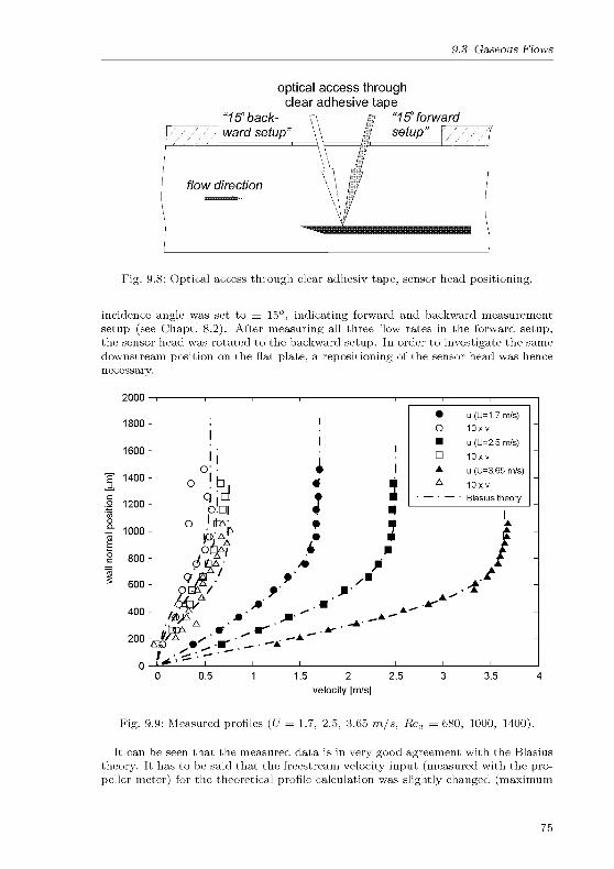
9.3 Gaseous Flows
optical access throughclear adhesive tape
"15? back¬
ward setup"
flow direction
"15° forward
setup"'
Fig. 9.8: Optical access through clear adhesiv tape, sensor head positioning.
incidence angle was set to ± 15°, indicating forward and backward measurement
setup (see Chapt. 8.2). After measuring all three flow rates in the forward setup,
the sensor head was rotated to the backward setup. In order to investigate the same
downstream position on the flat plate, a repositioning of the sensor head was hence
necessary.
2000 r
1800
1600
1" 1400
2,
| 1200
'55o
- 100003
E
i 800
"toä
600
400
200
0
1 1
• u (U=1 7 m/s)
o 10xv
! i,
u (U=2 5 m/s)
o'1 iD 10xv
u (U=3 65 m/s)
o !h « -
q,d • à
o!di 4 n
A10xv
Blasius theory
|o jit*- *
PA ,•
or^A, i m
9/8 * /*
A-'
.
fir s-*'* .-*-*'££> X«C- 'K- —
' ~~A
;*-, i i
0.5 1.5 2 2.5
velocity [m/s]
3.5
Fig. 9.9: Measured profiles (U = 1.7, 2.5, 3.65 m/s, Rex = 680, 1000, 1400).
It can be seen that the measured data is in very good agreement with the Blasius
theory. It has to be said that the freestream velocity input (measured with the pro¬
peller meter) for the theoretical profile calculation was slightly changed (maximum
75

9 Experiments
by ±0.1 m/s), in order to achieve the best fit with the measured profile. Never¬
theless, for the wall-parallel velocity component, only a few points show a small
deviation from the theoretical boundary layer shape (±1%). The agreement for the
out-of-plane velocity (scaled up in the plot by a factor of 10) is worse, but still satis¬
factory. Note that the measurement uncertainty (in absolute terms) is independentof the flow velocity. This leads to large relative errors for low flow velocities.
In contrast to the measurements in liquid, no retro-reflecting foil was used to
generate the reference reflection. Hence, the zero delay setting of the interferometer
is equal to the zero wall normal position. As mentioned before, for measurements
very close to the surface this leads to large beat signal due to interference of each
signal with itself. Therefore, measurements within the first 150 /im above the surface
could not be obtained. Since this value only depends on the light source, but is
independent of the flow, the spatial resolution in terms of wall units will depend
on the flow. For the intermediate flow speed of U = 2 5 m/s (Rex = 1000), this
corresponds to y+ fa 3 5. If desired, it would also be possible to use a retro-reflector
in gaseous flows, allowing measurements much closer to the wall. However, comparedto aluminum powder seeding used for the measurements in liquids, the salt crystalflow seeding produces a much weaker reflection. Due to this, only reflections of
salt particles very close to the focal point produce a detectable signal. In turn, the
positioning of the focal point right above the retro-reflector is very challenging as it
was done just by hand in these experiments.
76
10 Measurement Uncertainty Considerations
for SR-LDV
10.1 General Measurement Precision
Even though various error sources for laser-Doppler velocimetry are discussed in the
literature, e.g., (Durst et al., 1987) and references given there, the overall measure¬
ment error for a specific system and for a specific application is not easy to estimate.
In addition, to validate a new LDV sensor concept a simple theoretical model mightnot be feasible. Alternatively, validations are done experimentally by measuring a
well known phenomenon and comparing the results with the theory.
For the novel boundary layer profiler this was done with a number of generic flows,
i.e., a Poiseuille flow, a Taylor-Couette flow and a laminar Blasius boundary layerover a flat plate. The estimation of the errors in these specific experiments was done
under the assumption of a theoretical perfect flow (no turbulence). To compare
the test results the optical arrangement of the sensor head was not modified (lensdiameter 5 mm, measurement distance approx. 60 mm, observation angle ± 15°).
In general, a simple lower limit for the frequency measurement accuracy can be
given by
A/mm ~-*-
(10.1)
where At is the length of the observed particle burst. In particular, this could be
improved by a factor of about 2 due to the interpolation scheme for the peak detection
in the power spectrum. However, this value strongly depends on the experimental
setup and cannot be taken as constant. In the following only three sources of error
are described, which are significant for the self-referencing setup.
10.2 Aperture Broadening
As shown in Fig. 10.1, the angle of scattered light can vary from +/3 to —ß dependingon the aperture of the collecting lens. Since the Doppler shift of the backscattered
light among others also depends on the observation angle (see Eq. 3.2, Chapt. 3.2.2),this results in a broadening of the received Doppler frequency signal. In a first
77
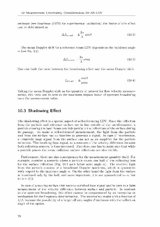
10 Measurement Uncertainty Considerations for SR-LDV
estimate (see Saanmaa (1979) for experimental validation) the limits of this effect
can be determined as
2-u
^fbroad = ±— Sinß (10.2)A
The mean Doppler shift for a reference beam LDV depends on the incidence anglea (see Eq. 3.5)
2m
Afmcan = —sma (10.3)A
One can built the ratio between the broadening effect and the mean Doppler shift
sinßCbroad = ± (10.4)
sma
Taking the mean Doppler shift as the quantity of interest for flow velocity measure¬
ments, this ratio can be seen as the maximum impact factor of aperture broadeningonto the measurement value.
10.3 Shadowing Effect
The shadowing effect is a special aspect of self-referencing LDV. Since the reflection
from the particle and reference surface are in line outside of the interferometer, a
particle crossing the laser beam can hide partially the reflections of the surface duringits passage. To make a self-referenced measurement, the light from the particleand from the surface has to interfere to generate a signal. In case of interference,
a relatively large signal from the surface can act as an amplifier for the particlereflection. The resulting beat signal, as a measure of the velocity difference between
both reflection sources, is thus increased. Therefore, one has to make sure that while
a particle passes the focus, sufficient surface reflections are also visible.
Furthermore, there are also consequences for the measurement quantity itself. For
example, consider a scenario where a particle covers one half of the collecting lens
for the surface reflection (Fig. 10.1 part below solid angle a). The received lightfrom the particle consists of a broadened Doppler spectrum, which is symmetricwith respect to the incidence angle a. On the other hand the light from the surface
is broadened only by the half, and more important, it is not symmetrical to a, but
to a - ß/2.
In case of a moving surface this leads to a shifted beat signal and in turn to a false
measurement of the velocity difference between surface and particle. In contrast
to the aperture broadening, this effect cannot be compensated by an interpolationmechanism for the frequency determination. The uncertainty scales with a fraction of
l/ß, because the possibility of a larger off axis angles ß increases with the collection
angle of the optics.
78
10.4 Frequency Resolution
collectinglens
surface
Fig. 10.1: Aperture broadening (black), shadowing effect (gray).
10.4 Frequency Resolution
As mentioned the frequency equivalent Afmm of the length of a given a beat sig¬nal defines the limits for the frequency determination. Although the resolution of a
calculated power spectrum itself depends on the number of samples of a measure¬
ment trace, the accuracy of the frequency determination of a burst signal within
this trace is not simply improved by increasing the sampling rate. True resolution
improvements are only possible with longer burst signals.
The duration of a signal burst is governed by the time a particle needs to pass
the laser beam. Because this time changes linearly with the velocity of the flow, this
error source is a relative value. Thus, at low flow velocities the frequency resolution is
higher, allowing more accurate velocity measurement (vice versa for high velocities).Besides of the velocity, the passage time of a particle through a laser beam only
depends on the diameter of the laser beam and on that of the particle. The largerof which is the determining factor.
Using larger seeding particles increases the passage time and in turn the frequency
resolution, as well as the amount of backrefiected light from the particles. However,
an upper limit for particle sizes is given by their inertia and hence their ability to
follow the flow. Changing the acceptance angle of a given collecting lens affects the
beam diameter in the focus. A smaller collecting angle produces a larger beam diam¬
eter, which in turn increases the particle passage time. On the other hand, a largebeam diameter decreases the light intensity in the focus. Together with the smaller
acceptance angle, the amount of light received from a particle decreases rapidly.
Ideally, the diameter of the laser beam and that of the particles are comparable and
as large as possible.
79

10 Measurement Uncertainty Considerations for SR-LDV
80
11 Conclusions / Outlook
11.1 Summary
Two optical velocimetry techniques were presented which are based on low coherence
interferometry. Both have in common that the extent and the error of the position of
the measurement volume are comparable to the coherence length of the light source
(tens of micrometers). They also share the features that the measurement location
is set relative to a reference surface (which could be the surface of a moving object),that they require particle seeding and that the measurement location can be scanned
along a line without mechanical movement of the sensor head. Multiple components
of the velocity vector can be measured using a single interferometer and light source.
Both techniques were demonstrated in proof-of-principle measurements for liquids.The measurement range depends on the power of the light source, the reflection levels
of the reference surface and the particles (i.e., particle size) and the collection angleof the optics (i.e., lens diameter and distance to the measurement volume). In the
first test series a lens with a diameter of 5 mm, a measurement distance of 60 mm
(collection angle of approx. 5 deg.), aluminum powder as particle seeding (approx.50 ßm in size) and a 10 mW light source (SLD, Superlum Diodes model SLD56-HP2)were used. This allowed a measurement range of approx. 4 mm, without moving
the sensor head. Improvements could be made using a more powerful light source
(Exalos EXS1320-1111, 25mW). For measurements in liquids the measurement range
was increased by a factor of 2. Hence, the focal point does not need to be located most
accurate to the surface, facilitating the handling of the sensor. With the increase
in light power, measurements in air could also be demonstrated. With a collection
angle of approx. 5° and small salt crystals as seeding (1-4 ßm in size) a measurement
range of approx. 2 mm without relocating the sensor head was possible.
Decreasing the collection angle leads to an elongated focal point, which in turn
increases the range in which the sensor front end does not need to be moved to
collect particle reflections, as well as the absolute measurement range in respect to
the surface. It also increases the accuracy of the velocity measurement, due to longer
lasting signals. On the other hand it significantly lowers the reflection level from the
particles. Due to the autocorrelator setup of the interferometer and the large zero
delay signal, measurements within the first 100 microns above the wall could not be
achieved directly. With the help of a retro-reflector on the surface, the measurement
location indicating the surface could be set away from zero interferometer delay.
Further developments should focus on the handling of the sensor. Although the
sensor has self-referencing capabilities, measurements are only possible when the fo¬
cus is set close to the surface, especially when using small particles as in air flows.
To overcome this limitation an auto-focusing optic should be implemented. Further-
81

11 Conclusions / Outlook
more, with the actual SR-LDV single beam setup the incident angle to the surface
must be known, which is a direct source of uncertainty.
In the following an alternative dual beam configuration for SR-LDV is brieflydescribed. The basic principle is the same as in the single beam arrangement, but
the system should be able to overcome the problems with the unknown incident
angle and the large zero delay signal.
11.2 Dual Beam Self-Referencing Laser Doppler Velocimeter
Fig. 11.1 shows the schematic setup of the optical components in the interferometer
unit of the proposed dual beam self-referencing system. A light source emits low
coherence light into a singlemode fiber. A fiber-optical isolator protects the sensitive
light source from backreflections and guides the light to a polarization insensitive
optical circulator. The circulator is used to transfer the light through a singlemode
optical fiber to the a beamsplitter, where the light is split into two parts of equal
intensity (denoted with rays a and b).
The light is guided through singlemode fibers to two coupling lenses in the sensor
head, lenses la and lb- The length of fiber a (lf,a) differs by design from that of fiber
b (lf,b) by a value Al, which must be significantly longer than the coherence lengthor any spatial quantity to be considered for a measurement (say, 10 cm).
—Q-
A/
SLD isolator circulator
o
acusto
opticmodulator
from / to sensor head
including two lenses
beam
splitter
variable
delayline
I photo diodes
Fig. 11.1 Dual beam self-referencing LDV interferometer design.
82

11.2 Dual Beam Self-Referencing Laser Doppler Velocimeter
incident beam
from lens a
incident beam
from lens b
oseeding particles
flow direction
surface of the object
Fig. 11.2: Dual beam self-referencing LDV principle.
Following the nomenclature of Fig. 11.2, light reflected off the test object surface
is denoted as rays la and 16 and the light scattered off the particles in the flow is
denoted as rays 2a and 26. All light backrefiected and collected by both lenses is
guided back to the beam splitter. There one half of the rays 1 and 2 is deflected to
the circulator and then into the reference arm including a acousto-optic modulator.
The other half is fed into the variable delay arm of the interferometer. The light from
the two interferometer arms is finally recombined by another beam splitter/combinerand a broadband photoreceiver serves as detector. In addition, there is an optionfor a second photoreceiver to increase the SNR.
It is assumed that both lenses have the same incidence angle to the surface, justwith an opposite sign, and that the surface is more or less reflective. For laser beam
a, as shown in Fig. 11.2, the light travels through the fiber a and is then focused
through the lens la onto the surface. There, part of the light a is deflected as ray la
to the lens lb- backreflections from a particle, ray 2a, will be collected by the lens
la- For laser beam 6 this will be vice versa, i.e., a surface reflection (16) is collected
by the lens a and a particle reflection (26) by lens 6.
However, all reflections (rays la, lb, 2a, 26) are now split into the two interfero¬
meter arms. Before the interferometer, the pathlength of rays la and 16 is the same
and equal to the length of the fiber a plus the fiber 6 and two times the distance
sensor head to surface dh.s The pathlength of ray 2a is twice the length of fiber a
plus the distance to the particle dhp. Finally, the pathlength of ray 26 is twice the
length of fiber 6 plus the distance to the particle. Since the lengths of the fibers
83

11 Conclusions / Outlook
differ by Al this can be summarized as
ha = hb = 21* + A I
ha = 2 (I* +Al)-2d*
l2b = 21* -2d*
with
Al =
f,a~ Lf,b,
h = lf,b + dhs,
d* = dhs - dhP
(11 la)
(11 lb)
(11 lc)
(11.2)
Setting the variable delay in the delay arm of the interferometer, various combi¬
nations of the subpairs of rays are possible. Thereby, only at a few the pathlengthsare equal and interference occurs. The following table gives a summary.
interferometer setting subpairs with equal pathlength
''delay — 're/subpairs interfere with their counterpart
and surface reflections ray la and 16
''delay= hef ~T 2> I 2b(delay) with 2a(ref)
''delay= hef ^ ' 2a(delay) with 2b(ref)
''delay= hef ~~r *> ~T 2 a 2b(delay) with la(ref), lb(ref)
''delay= hef ~~r *> 2 a la(delay), Ib(delay) with 2a(ref)
''delay= hef ' -\- 2 a 2a(delay) with la(ref), Ib(ref)
helay = hef ' ^ a> la(delay), Ib(delay) with 2b(ref)
Table 11.1 Combinations of the ray subpairs with equal pathlengths.
The procedure for data analysis of the dual beam SR-LDV is quite similar to
the analysis of the two independent measurements of the single beam SR-LDV (seeChapt. 8.2.2). If interference between a surface reflection and a particle reflection is
present, the difference of the Doppler shift frequency can be seen in the beat signal.
However, the different optical setup in the front end has to be considered in order
to relate the shift of the beat signal, / — fAOM, to the velocity components of the
particles in the flow.
84
11.2 Dual Beam Self-Referencing Laser Doppler Velocimeter
First, consider the wall-parallel velocity component u only and assume a flow
direction as shown in Fig. 11.2. The light backrefiected from the particles contains
a Doppler shift (rays 2a and 26). For the light rays 2a the Doppler shift is negative
(/2a = —2u/\)sina) and for the rays 26 it is positive (f2b = 2u/\)sina). The lightdeflected from the surface does not contain a Doppler shift. This is also true if
the surface is moving in u direction, because the light from the surface is deflected
from one lens to another with opposite angles. Therefore, this system measures the
wall-parallel velocity with respect to the sensor head.
For the wall-normal velocity component v, the system follows the descriptions
given Chapt. 8.2.2, which means this velocity component is measured relative to the
surface.
The orientation of the sensor head to the surface is inherently known, since suffi¬
cient surface reflections are only collected if the sensor head is oriented perpendicularto it.
85

11 Conclusions / Outlook
86

Appendix
87


Bibliography
AA-Opto-Eelectronic (2003). Apphation Notes Do you know Acousto-optics?
http //www.a-a.fr/Documentation/AO Doc.pdf. Technical report, last visited
Sept. 2006.
Albrecht HE Borys M Damaschke N Tropea C (2003). Laser Doppler and Phase
Doppler Measurement Techniques. Springer Verlag Berlin Heidelberg New York.
Alphonse CA Gilbert DB Harvey MG Ettenberg M (1988). High-power superlumi¬nescent diodes. Journal of Quantum Electronics 24 2454—2457.
ALSTOM Power (2006). GT24 and GT26 Gas Turbines - 188MW and 281MW.
http //www.power.alstom.com. last visited June 2006.
Barranger JR Ford MJ (1981). Laser Optical Blade Tip Clearance Measurement
System. J. Eng. Power 103(2) 457-460.
Behr T Kalfas AI Abhari RS (2006). Unsteady Flow Physics and Performance of a
One-and-l/2-Stage Unshrouded High Work Turbine. ASME Paper No. GT2006-
90959.
Böhm R Overbeck E (2005). Power as High as Lasers With the Optical Spectrumof a LED. Laser+Photomcs 5 28-30.
Booth TC (1985a). Turbine Loss Correlations and Analysis. VKI Lecture series
1985-5. Von Karman Institute, Rhode-St-Genese.
Booth TC (1985b). Importance of Tip-Clearance Flows in Turbine Design. VKI
Lecture series 1985-5. Von Karman Institute, Rhode-St-Genese.
Buttner L Czarske J (2001). A multimode-fiber laser-Doppler anemometer for highly
spatially resolved velocity measurements using low-coherence light. Measurements
Science and Technology 12 1891-1903.
Buttner L Czarske J (2003). Spatial resolving laser Doppler velocity profile sen¬
sor using sightly fringe systems and phase evaluation. Measurement Science and
Technology 14 2111-2120.
Cho HH Rhee DH Choi JH (2000). Heat/Mass Transfer Characteristics on Turbine
Shroud with Blade Tip Clearance. ICHMT Turbine-2000, Book of Abstracts, No.
32.
Coutsoukis P (2006). India Origin and Development, http //www.photius.com/countries/india/economy/. last visited Oct. 2006.
89

Bibliography
Dhadwal HS Kurkov AP (1999). Dual-laser probe measurement of blade-tip clear¬
ance. Journal of Engineering for Gas Turbines and Power 121 481—485.
Durst F Melhng A Whitelaw JH (1987). Theorie und Praxis der Laser-Doppler-Anemometrie. Braun, Karlsruhe.
Durst F Zanoun ES (2002). Experimental investigation of near—wall effects on hot¬
wire measurements. Experiments in Fluids 33 210—218.
Durst F Zanoun ES Pashtrapanska M (2001). In situ calibration of hot wires close
to highly heat—conducting walls. Experiments in Fluids 31 103—110.
Force Inc. (2006). Types of Optical Fiber, http //www.fiber-optics.info/articles/fiber-types.htm. last visited Sept. 2006.
Geisheimer J Bilhngton S Burgess D (2004). A microwave blade tip clearance sensor
for active clearance control applications. AIAA Paper No. 2004-3720.
Goodman JW (1988). Statistical Optics. John Wiley & Sons, Inc.
Gusmeroli V Martinelli M (1991). Distributed laser Doppler velocimeter. OpticsLetters 16 1358-1360.
Haggmark CP Bakchinov AA Alfredsson PH (2000). Measurements with a flow
direction boundary-layer probe in a two-dimensional laminar separation bubble.
Exp. Fluids 28 236-242.
Hecht J (2006). A Short History of Fiber Optics, http //www.sff.net/people/Jeff.Hecht/history.html. last visited Sept. 2006.
Huang D Swanson EA Lin CJ Shuman JS Stinson WG Chang W Hee MR Flotte
T Gregory K Puhafito CA Fujimoto JG (1991). Optical coherence tomography.Measurements Science and Technology 254 1178—1181.
Inphenix, Inc (2004). Superluminescent Light Emitting Diodes Device Funda¬
mentals and Reliability, http //www.inphenix.com/pdfdoc/Apphcation Notes for
SLEDs.pdf. Technical report, last visited July 2006.
Kahske R (1996). Geschichtliches und Aktuelles der Optik. 1. Staatsexamen
Lehramt, Theoretische Kernphysik, Universität Hamburg.
Lakshminaryayana B (1985). Tip Clearance Effects in Axial Turbomachines. VKI
Lecture series 1985-5. Von Karman Institute, Rhode-St-Genese.
Ligrani PM Bradshaw PH (1987). Spatial resolution and measurement of turbulence
in the viscous sublayer using subminiature hot-wire probes. Exp. Fluids 5 407—
417.
Lin HJ Perhn M (1998). Improved methods for thin, surface boundary layer inves¬
tigations. Exp. Fluids 25 431-444.
Mandel L (1959). Fluctuations of Photon Beams The Distribution of the Photo-
Electrons. Proc. Phys. Soc. 74 233-243.
90

Bibliography
Masters BR (1999). Early Development of Optical Low-Coherence Reflectometryand Some Recent Biomedical Applications. Journal of Biomedical Optics 4 236—
247.
Meinhart CD Wereley ST Gray MHB (2000). Volume illumination for two-
dimensional particle image velocimetry. Measurements Science and Technology11 809-814.
Pfau A (2003). Loss Mechanisms in Labyrinth Seals of Shrouded Axial Turbines.
ETHZ Thesis No. 15226.
Pfister T Buttner L Czarske J (2005). Laser Doppler profile sensor with sub-
micrometre position resolution for velocity and absolute radius measurements of
rotating objects. Measurements Science and Technology 16 627—641.
Rooth RA Hiemstra W (2001). A Fiber-Optic Tip-Shroud Deflection Measurement
System. J. Eng. Power 123(2) 359-362.
Rusch D Kempe A Rosgen T (2006). Seeding of high temperature air flow. Experi¬ments in Fluids, submitted 04-06.
Saanmaa R (1979). A laser Doppler velocimeter for surface velocity measurement.
J.Phys.E. 12 600-603.
Schaub UW Vlasic E Moustapha SH (1993). Effect of tip clearance on the perfor¬mance of a highly loaded turbine stage. AGARD-CP-537 Paper No. 29.
Schhchting H Gersten K (2000). Boundary-Layer Theory. Springer Verlag Berlin.
Schodl R (1991). Laser Transit Velocimetry. Von Karman Institute for Fluid Dy¬namics LS 1991-05 Laser Velocimetry, Rhode Island.
Sheard AG ODonnell SG Stnngfellow JF (1999). High temperature proximity mea¬
surement in aero and industrial turbomachinery. Journal of Engineering for Gas
Turbines and Power 121 167-173.
Sieverding C (1985). Tip-Clearance Effects in Axial Turbomachines. Lecture series
1985-5. Von Karman Institute, Rhode-St-Genese.
Sjolander SA (1997). Secondary and Tip-Clearance Flows in Axial Turbines. VKI
Lecture series 1997-1. Von Karman Institute, Rhode-St-Genese.
Steiner A (2000). Techniques for blade tip clearance measurements with capacitive
probes. Measurements Science and Technology 11 865—869.
Superlum Diodes Ltd (2005). Performance Sheet SLD-56-HP Very-High-Power SLDs
at 1310 nm. http //www.superlumdiodes.com/pdf/56hp.pdf. Technical report,
last visited Oct. 2006.
Tomlins PH Wank RK (2005). Theory, developments and applications of opticalcoherence tomography. Journal of Physics D 38 2519—2535.
UDT Sensors Inc. (2006). Photodiode Characteristics, http //www.udt.com. last
visited June 2006.
91

Bibliography
van de Hülst HC (1981). Light Scattering by Small Particles. Dover, New York.
Wolff S Brunner S Fottner L (2000). The use of hot-wire anemometry to investi¬
gate unsteady wake-induced boundary-layer development on a high-lift lp turbine
cascade. Journal of Turbomachinary 122 644—650.
Yeh Y Cummins HZ (1964). Localized Fluid Flow Measurements with an He-Ne
Laser Spectrometer. Appl. Phys. Letters 4 1768—178.
92
Epilogue
Between 1997 and 2002 I was studying mechanical engineering with a focus in
aerospace technology, turbine engines and rocket propulsion at the Technical Uni¬
versity of Dresden. This study included an internship at ABB Corporate Research
Ltd, Switzerland. There, I was involved in the development of a new electronic do¬
mestic gas meter, which gave me first insights into sensor technologies. Later, in my
diploma thesis at the ETH Zurich I made feasibility studies for a new optical tip
clearance sensor. This not just opened me the doors to the field of optic measuring
techniques, but it also gave my the opportunity for my doctoral study. So I could
work on the development of a sensor from the first idea to a working prototype.
In that project I was working together with ALSTOM Power at the new tip
clearance sensor, where we could perform first proof-of-pnnciple tests at an ALSTOM
large-scale power plant gasturbine GT26. It was the first time the tip clearance has
been monitored with high temporal resolution. A modified version of the sensor
system will be built at ALSTOM Power. Maybe in the future it will become an
integral part of gasturbines with options to active clearance control.
At the same time I was working on another project, namely self-referencing ve¬
locimetry. The working interferometer system from the tip clearance sensor should
be used for some kind of flow velocimetry. Today low coherence interferometry is
not very common in flow velocimetry. This might be due to an actual lack of power
of broadband light sources compared to narrowband lasers. In medicine, optical co¬
herence tomography has become a standard technique since many years. This mightbe due to the fact that optical power must be limited anyway in order to not damagethe tissue.
For velocimetry applications I have utilized a key advantage of low coherence inter¬
ferometry when using a reference outside of the interferometer and thereby makingthe system self-referenced with respect to it. With this for example, boundary layermeasurements at irregularly moving surfaces can be easily obtained. First feasibilitytests have been done with the system in liquids and in air. With a rise of power in
broadband light sources in the near future, I think self-referencing velocimetry can
become a powerful tool for boundary layer investigations.
Personally, summarizing my doctoral study at ETH Zurich I can look back to 4
years full of interesting experiences. Be it the ups and downs in the research itself,the testing at this hell of a machine GT26 at ALSTOM, the teaching assistance of
a class with 200 students or the interesting journey to Pasadena.
93

Epilogue
94

Curriculum Vitae
Andreas Kempe
Personal Data
date of birth September 7, 1977
place of birth Zwickau, Germany
citizenship German
Education
2006 PhD examination, ETH Zurich, Zunch/CH
2003 Visiting Researcher, California Institute of Technology & Viosense Ltd.
Pasadena/USA (4 months)
2002 PhD Student (supervisor Prof. Dr.-Ing. T. Rosgen),ETH Zurich, Zunch/CHDegree Dipl.-Ing. Maschinenbau, Vertiefung Luft-/Raumfahrttechmk,TU Dresden, Dresden/DDiploma thesis, ETH Zurich, Zunch/CH
2001 Internship, ABB Corporate Research Ltd, Baden/CH (9 months)
1997 Study of Mechanical Engineering with focus in Aerospace Technology,TU Dresden, Dresden/D
1996 Military duty paratroopers, Merzig/DUniversity-entrance diploma, Clara-Wieck Gymnasium, Zwickau/D
1993 German secondary school, Clara-Wieck Gymnasium, Zwickau/D
1985 School, Polytechnische Oberschule Biel, Zwickau/D
95