low coherence interferometry for central thickness measurement of rigid and soft contact lenses

Low coherence interferometry for central thickness measurement of rigid and soft contact lenses

I. Verrier1*, C. Veillas1 and T. Lépine1, 2

Université de Lyon, F-69003, Lyon, France Université de Saint Etienne, F-42000, Saint-Etienne, France

1 CNRS UMR 5516, Laboratoire Hubert Curien, 18, rue Benoît LAURAS 42000 Saint-Etienne, France 2 Institut d’Optique Rhône-Alpes, 18, rue Benoît LAURAS 42000 Saint-Etienne, France

*Corresponding author: [email protected]

Abstract: In this paper we propose contact lens central thickness measurement with a low coherence interferometry technique using either a SLED source or a broadband continuum generated in air-silica Micro-structured Optical Fiber (MOF) pumped with a picosecond microchip laser. Each of these sources associated with the interferometer provides, at the same time, good measurement resolution and quick signal recording without moving any optical elements and without need of a Fourier Transform operation. Signal improvement is performed afterwards by a numerical treatment for optimal correlation peaks detection leading to central thickness value of several contact lenses.

2009 Optical Society of America

OCIS codes: (120.0120) Instrumentation, measurement and metrology; (120.3180) Interferometry.

References and links

1. M. A. Marcus, J. R. Lee, H. W. Harris, and R. Kelbe, “Apparatus for measuring Material Thickness Profiles,” US Patent # 6067161 (2000).

2. M. A. Marcus, J. R. Lee, and H. W. Harris, “Method for measuring material thickness profiles,” US Patent # 6038027 (2000).

3. T. Blalock and S. Heveron-Smith, “Practical applications in film and optics measurements for dual light source interferometry,” Proc. SPIE 5589, 107-113 (2004).

4. B. E. Bouma and G. J. Tearney, Handbook of optical coherence tomography (New York: Marcel Dekker 2002).

5. J. M. Schmitt, “Optical Coherence Tomography (OCT): A review,” IEEE J. of Sel. Top. Quantum Electron. 5, 1205-1215 (1999).

6. A. F. Fercher, W. Drexler, C. K. Hitzenberger, and T. Lasser, “Optical coherence tomography principles and applications,” Rep. Prog. Phys. 66, 239-303 (2003).

7. R. Leitbeg, C. K. Hitzenberger, and A. F. Fercher, “Performance of Fourier domain vs. time domain optical coherence tomography,” Opt. Express 11, 889-894 (2003).

8. R. Leitbeg, M. Wojtkowski, A. Kowalczyk, C. K. Hitzenberger, M. Sticker, and A. F. Fercher, “Spectral measurement of absorption by spectroscopic frequency-domain optical coherence tomography,” Opt. Lett. 25, 820-822 (2000).

9. Y. Park, T. J. Ahn, J. C. Kieffer, and J. Azana, “Optical Frequency domain reflectometry based on real–time Fourier Transformation,” Opt. Express 15, 4597-4616 (2007).

10. C. Dorrer, N. Belabas, J. P. Likforman, and M. Joffre, “Spectral resolution and sampling issues in Fourier-Transform spectral interferometry,” J. Opt. Soc. Am. B 17, 1795-1802 (2000).

11. C. Dorrer, “Influence of the calibration of the detector on spectral interferometry,” J. Opt. Soc. Am. B 16, 1160-1168 (1999).

12. K. Ben Houcine, G. Brun, M. Jacquot, I. Verrier, D. Reolon, and C. Veillas, “Temporal analysis of optical complex structures: application to tomography through scattering media,” Proc. SPIE 5249, 526-533 (2004).

13. K. Ben Houcine, M. Jacquot, I. Verrier, G. Brun, and C. Veillas, “Imaging through scattering medium using SISAM correlator,” Opt. Lett. 29, 2908-2910 (2004).

14. V. Tombelaine, C. Lesvigne, P. Leproux, L. Grossard, V. Couderc, J. L. Auguste, J. M. Blondy, G. Huss, and P. H. Pioger, "Ultra wide band supercontinuum generation in air-silica holey fibers by SHG-induced modulation instabilities," Opt. Express 13, 7399-7404 (2005).

#107490 - $15.00 USD Received 11 Feb 2009; revised 19 Mar 2009; accepted 20 Mar 2009; published 15 May 2009

(C) 2009 OSA 25 May 2009 / Vol. 17, No. 11 / OPTICS EXPRESS 9157

15. I. Verrier, G. Brun, and J. P. Goure, “SISAM interferometer for distance measurement,” Appl. Opt. 36, 6 (1997).

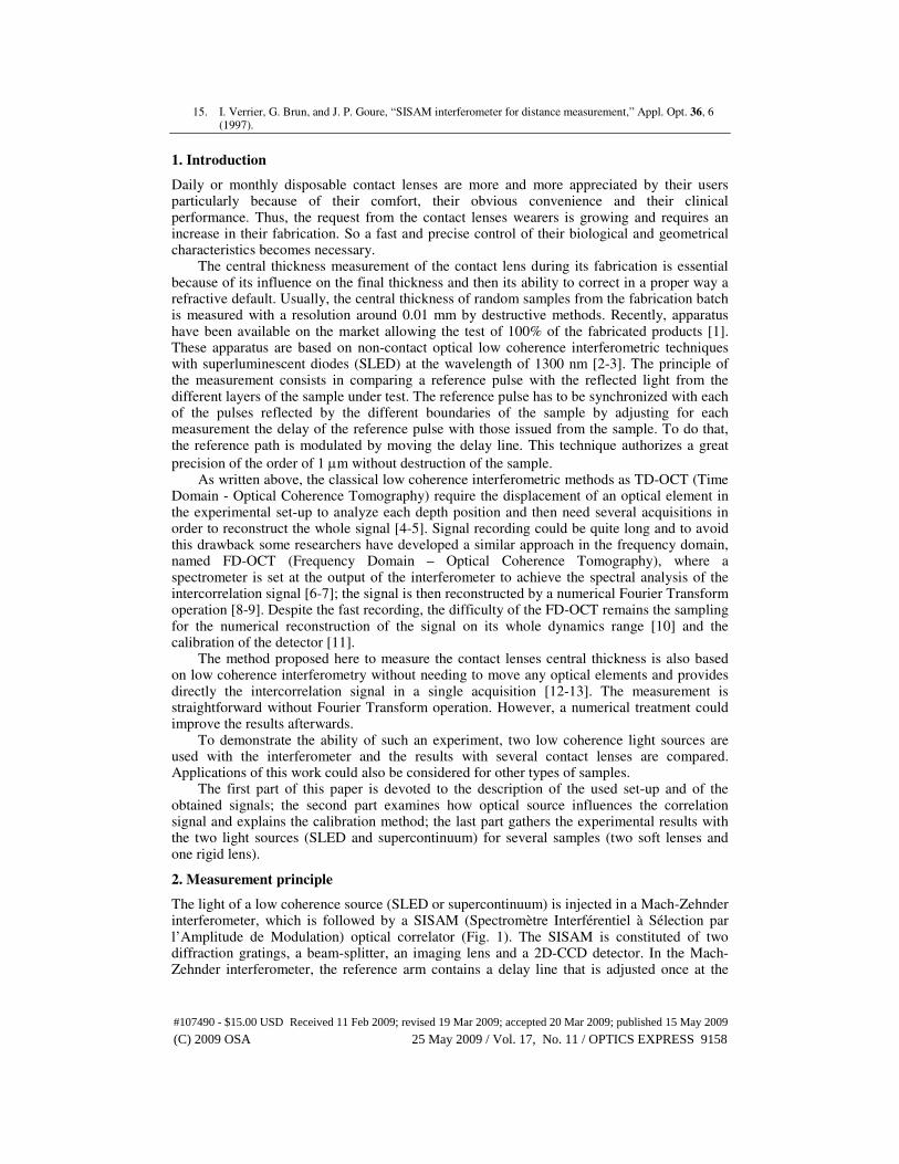
1. Introduction

Daily or monthly disposable contact lenses are more and more appreciated by their users particularly because of their comfort, their obvious convenience and their clinical performance. Thus, the request from the contact lenses wearers is growing and requires an increase in their fabrication. So a fast and precise control of their biological and geometrical characteristics becomes necessary.

The central thickness measurement of the contact lens during its fabrication is essential because of its influence on the final thickness and then its ability to correct in a proper way a refractive default. Usually, the central thickness of random samples from the fabrication batch is measured with a resolution around 0.01 mm by destructive methods. Recently, apparatus have been available on the market allowing the test of 100% of the fabricated products [1]. These apparatus are based on non-contact optical low coherence interferometric techniques with superluminescent diodes (SLED) at the wavelength of 1300 nm [2-3]. The principle of the measurement consists in comparing a reference pulse with the reflected light from the different layers of the sample under test. The reference pulse has to be synchronized with each of the pulses reflected by the different boundaries of the sample by adjusting for each measurement the delay of the reference pulse with those issued from the sample. To do that, the reference path is modulated by moving the delay line. This technique authorizes a great

precision of the order of 1 µm without destruction of the sample. As written above, the classical low coherence interferometric methods as TD-OCT (Time

Domain - Optical Coherence Tomography) require the displacement of an optical element in the experimental set-up to analyze each depth position and then need several acquisitions in order to reconstruct the whole signal [4-5]. Signal recording could be quite long and to avoid this drawback some researchers have developed a similar approach in the frequency domain, named FD-OCT (Frequency Domain – Optical Coherence Tomography), where a spectrometer is set at the output of the interferometer to achieve the spectral analysis of the intercorrelation signal [6-7]; the signal is then reconstructed by a numerical Fourier Transform operation [8-9]. Despite the fast recording, the difficulty of the FD-OCT remains the sampling for the numerical reconstruction of the signal on its whole dynamics range [10] and the calibration of the detector [11].

The method proposed here to measure the contact lenses central thickness is also based on low coherence interferometry without needing to move any optical elements and provides directly the intercorrelation signal in a single acquisition [12-13]. The measurement is straightforward without Fourier Transform operation. However, a numerical treatment could improve the results afterwards.

To demonstrate the ability of such an experiment, two low coherence light sources are used with the interferometer and the results with several contact lenses are compared. Applications of this work could also be considered for other types of samples.

The first part of this paper is devoted to the description of the used set-up and of the obtained signals; the second part examines how optical source influences the correlation signal and explains the calibration method; the last part gathers the experimental results with the two light sources (SLED and supercontinuum) for several samples (two soft lenses and one rigid lens).

2. Measurement principle

The light of a low coherence source (SLED or supercontinuum) is injected in a Mach-Zehnder interferometer, which is followed by a SISAM (Spectromètre Interférentiel à Sélection par l’Amplitude de Modulation) optical correlator (Fig. 1). The SISAM is constituted of two diffraction gratings, a beam-splitter, an imaging lens and a 2D-CCD detector. In the Mach-Zehnder interferometer, the reference arm contains a delay line that is adjusted once at the



beginning and that keeps the same position during the acquisition; the sample is set in the measurement arm at the focal point of a microscope objective.

Fig. 1. Set-up.

2.1 Low coherence sources

The light source used here is either a SLED emitting at the central wavelength λ0 = 822.4 nm

over a spectral bandwidth of ∆λ = 39 nm (full width at 1/e2) connected to a monomode fiber

or a source emitting a supercontinuum light over the visible spectrum up to the near infrared

region (flat spectrum around λ0 = 1064 nm of full width ∆λ = 1580 nm between the minima) generated in an air-silica Microstructured Optical Fiber (MOF) pumped by a picosecond microchip laser [14].

The wave amplitude after collimation by the lens at the interferometer input is expressed as:

Sc = Ss r( )Γ ν( ) (1)

Ss r( ) is the spatial distribution amplitude where r

2 = x2 + y2 is the radial component and

Γ ν( ) is the temporal frequencies distribution.

The beam is supposed to be spatially Gaussian for the SLED and with a first order Bessel distribution for the supercontinuum. Indeed, the fiber propagates only the fundamental mode for the wavelengths associated to the SLED and the MOF inside which is generated the supercontinuum propagates only the LP11 mode in the visible range. Then, for each source, the spatial distribution is:

SLED:

Ss r( )= S0 exp −r2

a02

a0 ≈ 1mm

Supercontinuum:

Ss r( )= S0J1

r

a1

a1 = 2mm (2)

a0 and a1 stand, respectively, for the beam radius of the fundamental mode and for the

dimension of the LP11 mode after propagation up to the collimating lens.

J1

r

a1

is the first

order Bessel function.

Lens

Inter-correlation

Beam-splitter Beam-splitter

Grating 1

Detector

x

y z

Object under test

Lens

Beam-splitter

Grating 2

Delay line Mirror

Mirror Mirror

Source

Microscope objective

Φ = 2 mm



The temporal frequencies spectrum Γ ν( )= TF γ t()( ) of each light source is such as its

distribution is Gaussian for the SLED and flat for the supercontinuum:

SLED:

Γ ν( )2 = Γ0

2exp −4

ν −ν0( )2

∆ν 2

with

ν0 = 3.646 1014 Hz

∆ν1/ e2 =c

λ0

2∆λ = 1.73 1013 Hz

Supercontinuum: Γ ν( )

2= Γ0

2

∀ν ∈ 1.7;7[ ]1014 Hz (3)

2.2 Mach-Zehnder interferometer

In the reference arm, the wave propagates in air up to the first diffraction grating and remains

nearly collimated. Its phase ϕR ν( ) is proportional to the traveling path lR:

ϕR ν( )=

2πνc

lR (4)

In the measurement arm, the wave propagates in air up to the 10x microscope objective, is focalized and reflected back by each interface of the object. Then, the different waves still

travel in air up to the second diffraction grating. The phase ϕ i ν( ) of each reflected wave is

expressed as:

ϕ i ν( )=2πν

clT + 2 nk ek

k =1i>1

i−1

∑

(5)

where lT, nk, ek are respectively the total path in air, the refractive index and the thickness of the object slice k.

The amplitude distributions SR and Si traveling up to each grating are then given by:

SR r,ν( )= αRSs r( )Γ ν( )exp − j2πν

clR

Si r,ν( )=αT Ss r( )Γ ν( )ri tk2

k=1i>1

i−1

∏

exp − j

2πνc

lT +2 nk ek

k=1i>1

i−1

∑

(6)

The coefficients αR and αT correspond to the reflected and transmitted waves amplitudes by the different beam-splitters for each arm of the interferometer. ri is the reflection amplitude coefficient of the last interface i. For each slice k, the transmission amplitude coefficient is tk.

Assuming that the object is constituted of only one slice (2 interfaces), then the whole amplitude wave in the measurement arm just behind the second grating is:

ST r,ν( )= S1 r,ν( )+ S2 r,ν( )= Si r,ν( )i=1

2

∑

=αT Ss r( )Γ ν( )r1 exp − j2πν

clT

+ r2t1

2exp − j

2πνc

lT + 2n1e1( )

(7)

In the case of same media in front of and behind the object, then the reflection amplitude coefficients r1 and r2 are equal (r1=r2=r) leading to the reflection intensity coefficient R=rr* and to the transmission intensity coefficient T=1-R.

Each interface induces a pulse that propagates up to the second diffraction grating.



2.3 SISAM correlator

The fields of the different waves propagated in the Mach-Zehnder interferometer undergo a phase shift by the two SISAM gratings in an antisymmetrical way in each arm. The induced

phase shifts are respectively ψR r,ν( ) and

ψT r,ν( ) for the reference and the measurement

arms. These waves are then added by the beam-splitter onto the CCD detector. The resulting

amplitude S r,ν( ) is the sum of the waves phase-shifted by the object and the gratings:

S r,ν( )= SR r,ν( )exp jψR r,ν( )[ ]+ ST r,ν( )exp jψT r,ν( )[ ] (8)

The integral of the power spectral density CSS r,ν( ) of the resulting wave

S r,ν( ), on the

whole source frequency bandwidth, yields to the light distribution EC r( ) at the output of the

SISAM:

EC r( )= CSS r,ν( )dν

ν∫ = S r,ν( )S∗ r,ν( )ν∫ dν (9)

CSS r,ν( ) is the autocorrelation function of the resulting wave

S r,ν( ):

CSS r,ν( )= SR r,ν( )

2

+ ST r,ν( )2

+ SR r,ν( )ST

∗r,ν( )exp − j∆ψ( )+ SR

∗r,ν( )ST r,ν( )exp j∆ψ( )

(10)

The phase difference ∆ψ =ψT −ψR due to the diffraction gratings is developed at the first

order around the central frequency ν0 and is expressed as:

∆ψ = ψT −ψR = 2π

⌣

Q + Qν( )X

with

⌣

Q =2N0

cos ′ θ 0cos ′ θ p − ′ θ 0( )

and

Q = 2 −N0

ν0 cos ′ θ 0cos ′ θ p − ′ θ 0( )+

1

csin ′ θ p − ′ θ 0( )

(11)

X is the horizontal coordinate (perpendicular to the grating lines) bound to the detector. The mathematical definition of X and calculation steps of Eq. (11) have been already developed [15]. The lens at the output of the SISAM images the two gratings planes onto the 2D-CCD camera with a magnification equal to 1.

N0 = 150 l/mm is the lines number per millimeter of each grating, ′ θ 0 the diffraction angle

for the source central wavelength λ0 and

′ θ p the diffraction angle corresponding to the flat tint

(beams are parallel and superposed) at the wavelength λ p

. The incidence angle upon the

gratings is θ0 = 82.5°. In order to add the beams after the gratings, the beam-splitter is set at

45° from each diffracted beam at the wavelength λ p (flat tint) (Fig. 2).

Fig. 2. Beams addition.

As a matter of fact, the SISAM plays the role of correlator between the measurement and reference fields by their direct temporal intercorrelation in real time without moving the delay

Grating 1

Detector

X

Z

Lens

Beam-splitter

Grating 2 θ’p θ0

θ’0

Y



line. The phase shift induced by the two diffraction gratings on each wave transverse section permits then to avoid the modulation of the reference optical path contrary to TD-OCT and does not need any numerical Fourier Transform operation, as it is the case for FD-OCT.

The light distribution on the detector is finally written as:

Ec X( )= E0 1+ K

′ K cos 4πν0

n1e1

c

F π∆ν 2n1e1

c

+cos4πν0

cX sin ′ θ p − ′ θ 0( )+ 2πν0

∆l

c

F π∆ν

∆l

c+ QX

+T cos4πν0

cX sin ′ θ p − ′ θ 0( )+ 2πν0

∆l + 2n1e1

c

F π∆ν ∆l + 2n1e1

c+ QX

(12)

with:

K =2αRαT R

αR2 +αT

2 R 1+ T 2( )′ K =

αT

αR

T R ∆l = lT − lR

E0 = S02Γ0

2∆ν αR2 +αT

2 R 1+ T 2( )[ ]J1

r

a1

π2

exp −r2

a02

and

F x( )=

sinc x( )=sin x

xcontinuum

exp −x

2

2

SLED

Equation (12) exhibits 3 terms:

• A continuous background

E0 1+ K ′ K cos 4πν0

n1e1

c

F π∆ν

2n1e1

c

;

• A first vertical correlation peak centered at

X0 = −∆l

cQ of full width:

∆X =2

∆νQ

between the minima for the supercontinuum and

∆X =2

π2

∆νQ at 1/e

2 for the SLED;

• A second vertical correlation peak centered at

X1 = −∆l + 2n1e1

cQ of same full width.

The two correlation peaks have nearly the same width depending on the source spectral

width ∆ν and on the Q factor induced by the SISAM: the greater the source spectral

bandwidth ∆ν and the factor Q are, the thinner the peaks are. The Q factor, when developed

at the first order, varies in the same way as N0, θ0 and (λ0)-1

. It can be deduced that the correlation peaks are thinner when the source spectral

bandwidth ∆ν, the incidence angle θ0 on the grating and the grating dispersion are increasing

(N0 high) and when the central wavelength λ0 is decreasing. However, the light distribution at the set-up output has been calculated with an approximation of the phases induced by the SISAM gratings since the phase difference development of Eq. (11) is limited to the first order; the dispersion terms of higher orders lead to phase distortion. Furthermore, the microscope objective in front of the sample induces additional dispersion that contributes to correlation peaks broadening in particular for very broadband spectrum such as the supercontinuum source.

The peaks are centered at the group delays of each of the reflected waves by the object and are weighted by the SISAM scale factor Q that imposes then the measurement range and

the resolution. Moreover these peaks are spatially modulated at

2ν0

csin ′ θ p − ′ θ 0( ) frequency

leading to a greater oscillations number in the peaks when the temporal central frequency ν0

and the diffraction angles difference θp’-θ0’ are growing. The peak location is chosen at the maximum of the oscillations envelop.



3. Correlation signals, calibration and limits of the set-up

3.1 Correlation signals, numerical treatment and calibration

As explained in the section 2, the signal captured by the 2D-CCD detector (Sony XC-EI50CE) does not only depend on the SISAM configuration but also on the selected optical source (SLED or supercontinuum). At first, to show how the source influences the correlation signal, a mirror is used as object and set at the focal plane of the microscope objective. The delay line is kept at a fixed position so that the two arms of the interferometer are nearly equal. Then, the 2D-CCD camera records a correlation signal for the SLED (Fig. 3(a)) or the supercontinuum (Fig. 3(b)) light sources.

(a) (b)

Fig. 3. Correlation images with (a) the SLED source and (b) the supercontinuum.

Each of the two signals exhibits, inside its envelope, only one vertical correlation peak due to the interferences between the reference pulse and the single reflected pulse by the mirror. The spatial envelop of the light distribution differs for the SLED and the supercontinuum (Eq. (12)): the SLED one is a Gaussian function and is maximum at the centre of the camera whereas the supercontinuum one varies as a first order Bessel function and reveals two sides lobes along the y-axis with a minimum at its centre.

In order to improve the correlation signal, a numerical treatment has been developed with Matlab in the following manner. The signals corresponding to the measurement and reference arms are also recorded separately and subtracted from the correlation signal in order to suppress the continuous background (Figs. 4(a) and 4(d)).

Fig. 4. Determination of the correlation peaks. (a) Subtracted image with the SLED. (b) Vertical filter and region of interest with the SLED. (c) Columns sum with the SLED. (d) Subtracted image with the supercontinuum. (e) Vertical filter and region of interest with the supercontinuum. (f) Columns sum with the supercontinuum.

Correlation peak Correlation peak

Y vertical pixel number

X horizontal pixel number

X horizontal pixel number

Y vertical pixel number

(c) (b) (a)

(f) (e) (d) n° 363 n° 407 X X

n° 409 n° 417 X

y

X

y

y y X

Grey level sum (a.u.)

X




A region of interest of the subtracted signal is then selected and a vertical Prewitt filter (method for edge detection) is applied to this region for extraction of the strong contrast areas (Figs. 4(b) and 4(e)). A sum over the columns and suppression of linear tendency part by part allows enhancing the signal. Then, each peak is automatically detected by search of the maxima inside the signal envelop (Figs. 4(c) and 4(f)) in the following way: all the values exceeding a threshold are taken into account. The threshold is chosen to be as three times the sliding standard deviation calculated with the values immediately before the considered point.

The peak maximum and the standard deviation expressed in grey level sum are 2300 and 60 for the SLED (Fig. 4(c)) whereas these values are 5900 and 50 for the supercontinuum (Fig. 4(f)). It leads to SNR equal to 16 dB for the SLED and 21 dB for the supercontinuum.

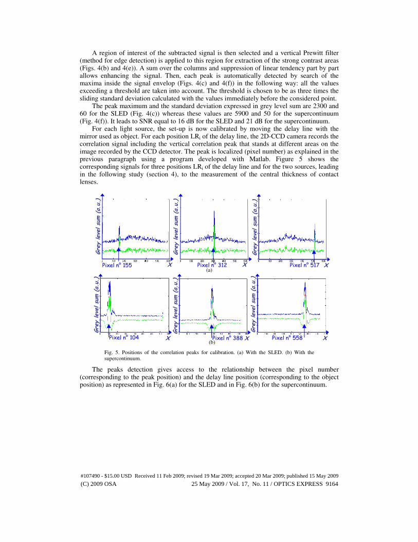
For each light source, the set-up is now calibrated by moving the delay line with the mirror used as object. For each position LRi of the delay line, the 2D-CCD camera records the correlation signal including the vertical correlation peak that stands at different areas on the image recorded by the CCD detector. The peak is localized (pixel number) as explained in the previous paragraph using a program developed with Matlab. Figure 5 shows the corresponding signals for three positions LRi of the delay line and for the two sources, leading in the following study (section 4), to the measurement of the central thickness of contact lenses.

(a)

(b)

Fig. 5. Positions of the correlation peaks for calibration. (a) With the SLED. (b) With the supercontinuum.

The peaks detection gives access to the relationship between the pixel number (corresponding to the peak position) and the delay line position (corresponding to the object position) as represented in Fig. 6(a) for the SLED and in Fig. 6(b) for the supercontinuum.

Pixel n° 155 Pixel n° 517 Pixel n° 312

Pixel n° 104 Pixel n° 558 Pixel n° 388

X X


X

X X X








SLED source y = 0.001924x + 7.537430

R 2 = 0.999807

7.8

7.9

8

8.1

8.2

8.3

8.4

8.5

8.6

8.7

100 200 300 400 500 600

Pixel number X

Supercontinuum source

y = 0.0017980x + 18.1299339

R2 = 0.9998919

18 18.2 18.4 18.6 18.8 19 19.2 19.4

0 200 400 600 800 Pixel number X

Fig. 6 Calibration curves for the two sources (a) SLED. (b) supercontinuum.

These calibration curves lead to a conversion coefficient of 1.798 µm/pixel for the

supercontinuum and of 1.924 µm/pixel for the SLED.

3.2 Resolution, accuracy and measurement range

The calibration of the set-up when using the SLED or the supercontinuum source enables us now to compare, in term of optical paths, the peaks width that induces the resolution of the measurement. These theoretical values of the peaks widths between two minima for the supercontinuum are deduced from Eqs. 11 and 12 and given by:

∆X =2λ0

2

c∆λQ=

λ0

2

∆λ−

N0λ0

cos ′ θ 0cos ′ θ p − ′ θ 0( )+ sin ′ θ p − ′ θ 0( )

−1

(13)

For the SLED, Eq. (13) has to be multiplied by the coefficient 2 π when the peak width

is estimated at 1/e2. The numerical values of λo and ∆λ are firstly depending on the two

sources but also on the CCD detector which bandwidth can reduce the wavelength spectrum. In our case, the CCD spectral bandwidth is [300 – 1000 nm] which includes the wavelength spectrum of the SLED but not that of the supercontinuum. Taking into account the spectral

limitation of the CCD detector leads to the values of λo = 650 nm and ∆λ = 700 nm for the

supercontinuum whereas for the SLED, these values λo = 822.4 nm and ∆λ = 39 nm are staying the same as those of the source. The wavelength values corresponding to the flat tint

are λp = 632.5 nm (alignment with an HeNe) for the SLED and λp = λo = 650 nm for the supercontinuum. Then, with the help of the above numerical values, the theoretical widths of

the correlation peaks are calculated: ∆X = 59µm = 7 pixels (1 pixel = 8.6 µm on the detector)

for the SLED and ∆X = 3µm = 0.35 pixel for the supercontinuum. Here, it can be noticed that,

for the SLED, the correlation signal is well sampled, as the peak width is greater than two pixels. It is not the case for the supercontinuum, whose correlation signal retrieval could be critical as its width is smaller than one pixel. However, the sampling will not be a limitation, even for the particular case of the supercontinuum, because actually its correlation peak broadens as seen in the following paragraph.

The peak widths theoretical values are now compared with the experimental ones. The full width at 1/e

2 of the correlation peak for the SLED is measured to be 8 pixels (Fig. 4(c))

corresponding to an optical path difference of ∆δ = 15 µm (see calibration in Fig. 6), whereas

for the supercontinuum, the peak full width is of 44 pixels or ∆δ = 79 µm (Fig. 4(f)). Thus, the experimental peak width value is close to the theoretical one for the SLED contrary to the values for the supercontinuum. Indeed, when the optical frequency bandwidth becomes very large (case of the supercontinuum), the correlation peak undergoes broadening due to dispersion effect. This is not taken into account in Eq. 13 because the dispersion terms of high orders induced by the gratings, that contribute to phase distortion, have been omitted as well



as the dispersion induced by the microscope objective. As a result, the experimental correlation peak for the SLED is clearly getting thinner than that of the supercontinuum.

These experimental values of the correlation peak widths do not affect the accuracy and then the measurements results even in the case of the supercontinuum because the peak is always detected by the same criteria (search of the maximum of the oscillations envelop by the Matlab program). But the peak widths lead to the determination of the set-up resolution as established in the following paragraph.

a) Resolution

Let us consider now the case of different optical paths to be determined in the measurement arm, several intercorrelation peaks will then appear. To differentiate among them, the peaks of

spatial width ∆X must be well separated in order to be detected by the camera. Limitation to resolve the peaks is given at first sight by the Rayleigh criteria: the peaks separation must be greater than their half width (at 1/e

2 for the SLED or between the minima for the

supercontinuum). This condition implies that the path difference (δ = n1e1) is large enough

and greater than δmin = ∆δ/2 = 8 µm for the SLED and δmin = ∆δ/2 = 40 µm for the supercontinuum. The resolution of the set-up is then better for the SLED than for the supercontinuum.

b) Measurement range

Another point to be considered in the set-up is the maximum optical path difference that can be measured. The measurement range gives this upper limit of the optical path difference that should not exceed the maximum value corresponding to the camera field of 768 pixels. Indeed, in our experiment, the horizontal width of the beam is not a limiting factor to the

measurement range. Then the optical path difference must not be greater than δmax = 1.48 mm

(768 pixels) for the SLED and δmax = 1.4 mm (768 pixels) for the supercontinuum (see the corresponding conversion coefficients subsection 3.1). The measurement range is nearly the same for both sources.

c) Accuracy

The last limit presented here is the measurement accuracy that is fixed by the ability of the Matlab program to localize one correlation peak. The peak width does not influence the accuracy of the measurement much whereas the signal to noise ratio (SNR) is a limiting factor. Indeed, the position of the correlation peak is determined with a better accuracy if SNR is as high as possible. For the supercontinuum, the signal to noise ratio could be enhanced by suppression of the area in between the two lobes of the envelop signal (Fig. 4(e)). This central area does not bring any information about the signal and reduces the signal to noise ratio when the sum is achieved on the signal columns.

To quantify the set-up accuracy, a set of ten correlation signals has been recorded under the same experimental conditions. The numerical process is applied to each of the ten signals in order to compare the position of the correlation peak. At worst, the maximum of the correlation peak is localized at one pixel around + 1 pixel. Thus, the set-up accuracy is

considered to be of 3 pixels corresponding to an optical path of 5 µm for the supercontinuum

and 6 µm for the SLED (see the corresponding conversion coefficients subsection 3.1). In the

section 4, the accuracy is considered to be the same (6 µm) for the SLED and the supercontinuum.

The limits of the set-up being known, measurements with different samples can be now realized in order to validate the set-up.



4. Experimental results

Three contact lenses are tested in air: two soft lenses and a rigid one. Soft contact lenses refractive index and center thickness significantly depend on their water content. So for all the experiments, the lenses are taken out of their solution and immediately set into a box with their apex in front of the objective. The measurement takes a few seconds so that the lenses have no time to suffer from dehydration and are considered as wet.

4.1 Soft contact lens (-3.75D)

The first measured sample is a soft contact lens of optical power -3.75D made in Balafilcon A material. The mean values of the central thickness and refractive index given by the

manufacturer are roughly e1 = 90 µm and n1 = 1.4. As explained in subsection 3.1, the CCD detector records three images (one for the

correlation, one for the measurement signal and one for the reference signal). The interferences signal is extracted and shows two correlation peaks issued from the two contact lens interfaces.

Figure 7(a) shows the correlation signal after subtraction and numerical treatment when using the SLED source. It permits to obtain the following results: the positions of the two peaks induced by each faces of the lens are localized on the pixels which numbers are

X0 = 318 and X1 = 387. The optical path difference δ = n1e1 is corresponding to 69 pixels

leading to the lens central thickness. So, δ = 131 + 6 µm and e1 = 131/1.4 = 95 + 4 µm. For the supercontinuum source (Fig. 7(b)), the two correlation peaks, corresponding to

the two lens interfaces, are separated by 72 pixels meaning that e1 = 93 + 4 µm.

Fig. 7. Results for the soft lens of -3.75D. (a) with the SLED, (b) with the supercontinuum.

For both of the sources (SLED and supercontinuum), the experimental values of the

central lens thickness agree with the one given by the manufacturer (roughly 90 µm).

(b)

Pixel n° 318 Pixel n° 387


X X



X X

(a)

y

y



4.2 Soft contact lens (-4.75D)

The second sample is a soft contact lens fabricated in the same material (Balafilcon A) as the first lens but with an optical power of -4.75D. Measurements are realized in the same way as for the first sample. The mean values of the central thickness and refractive index are also

roughly e1 = 90 µm and n1 = 1.4. Figure 8(a) gives the numerical treatment of the correlation signal when using the SLED

source and leads to the following results: the two correlation peaks induced by each of the lens interfaces are localized on the pixels which numbers are X0 = 312 and X1 = 378 and the

central thickness is e1 = 91 + 4 µm. It has to be noticed that the small peak (around the pixel n°110) detected by the program is not significant and must not be taken into account.

(a)

(b)

Fig. 8. Results for the soft lens of -4.75D. (a) with the SLED, (b) with the supercontinuum.

For the measurement with the supercontinuum source (Fig. 8(b)), the gap between the two correlation peaks corresponding to the lens interfaces is of 78 pixels leading to

e1 = 101 + 4 µm and is greater than the expected value (nearly 90 µm) whereas the

measurement with the SLED source agrees with the value given by the manufacturer. This could be explained by the fact that, in the case of the supercontinuum, the reference beam is not strictly superimposed on the measurement one in the vertical direction.

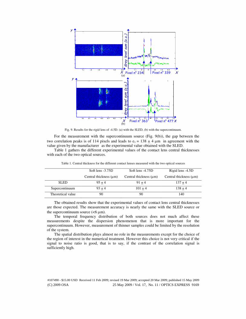
4.3 Rigid contact lens (-4.5D)

The last studied sample is a rigid contact lens of optical power -4.5D and fabricated in SiloxanyIMA-fluoroMA-MMA material. The mean values of its central thickness and

refractive index are roughly e1 = 140 µm and n1 = 1.48. Figure 9(a) shows the signal when using the SLED source and the two correlation peaks

corresponding to each lens interfaces are localized on the pixels which numbers are X0 = 234

and X1 = 339 corresponding to the lens central thickness of e1 = 137 + 4 µm.



X

y

X



(a.u.)

X

y

X



(a)

(b)

Fig. 9. Results for the rigid lens of -4.5D. (a) with the SLED, (b) with the supercontinuum.

For the measurement with the supercontinuum source (Fig. 9(b)), the gap between the

two correlation peaks is of 114 pixels and leads to e1 = 138 + 4 µm in agreement with the value given by the manufacturer as the experimental value obtained with the SLED.

Table 1 gathers the different experimental values of the contact lens central thicknesses with each of the two optical sources.

Table 1. Central thickness for the different contact lenses measured with the two optical sources

Soft lens -3.75D

Central thickness (µm)

Soft lens -4.75D


Rigid lens -4.5D


SLED 95 + 4 91 + 4 137 + 4

Supercontinuum 93 + 4 101 + 4 138 + 4

Theoretical value 90 90 140

The obtained results show that the experimental values of contact lens central thicknesses are those expected. The measurement accuracy is nearly the same with the SLED source or

the supercontinuum source (<6 µm). The temporal frequency distribution of both sources does not much affect these

measurements despite the dispersion phenomenon that is more important for the supercontinuum. However, measurement of thinner samples could be limited by the resolution of the system.

The spatial distribution plays almost no role in the measurements except for the choice of the region of interest in the numerical treatment. However this choice is not very critical if the signal to noise ratio is good, that is to say, if the contrast of the correlation signal is sufficiently high.

y



X X



X

y

X



5. Conclusion

In this work, the ability to measure contact lenses central thickness with a good accuracy is demonstrated. Two soft contact lenses and one rigid contact lens of close optical power have been used as samples with two different optical sources. The resolution of the measurements is more efficient for the SLED configuration than for the supercontinuum but the results are

nearly the same for each of the optical sources in terms of accuracy (around few µm). However, the resolution of the measurement can be enhanced in the case of the supercontinuum by compensating the dispersion induced by the microscope objective. This will be done in future work by inserting a similar objective in the reference arm. The numerical treatment itself is well adapted as, for the two sources configurations (SLED or Supercontinuum), the correlation peaks are well contrasted. Although, in the particular case of the supercontinuum, the numerical treatment could even take more advantage of a better choice of the region of interest by suppression of the beam central part where the light intensity is minimum.

In the final analysis, the indisputable advantage of this measurement technique is the very fast correlation signal recording since there is neither wavelength tuning nor delay line modulation.

Acknowledgments

The supercontinuum source was provided by Leukos in the frame of a collaboration with Xlim institute from Limoges (France) and the authors would like to express their thanks to V. Couderc, G. Huss et P. Leproux. The authors are also grateful to C. Fallet, student at the Institut d’Optique, for the elaboration of the computing program.



low coherence interferometry for central thickness measurement of rigid and soft contact lenses

Documents