looking inside mechanistic models of carcinogenesis

l

Looking inside mechanistic models ofcarcinogenesis

Sascha Zöllner

Helmholtz Zentrum München (Germany)Institute of Radiation Protection

l

Motivation

• Qualitative behavior?• Why do we needmechanistic model?

l

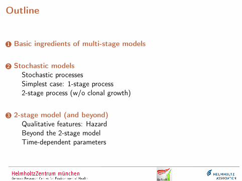
Outline

1 Basic ingredients of multi-stage models

2 Stochastic modelsStochastic processesSimplest case: 1-stage process2-stage process (w/o clonal growth)

3 2-stage model (and beyond)Qualitative features: HazardBeyond the 2-stage modelTime-dependent parameters

l




l

Modeling cancer: Key ingredients

(epi)genetic transitions: X0µ→ X1

µ→ ··· µ→ Xk

dXk

dt= µXk−1 =⇒ Xk(t) =

∫ t

0dt ′Xk−1µ

(...)= X0(µt)k/k!

[Armitage/Doll (1957)] polynomial growth

clonal expansion of pre-malignant cells: X1γ X1 +1

dX1

dt= γX1 =⇒ X1(t) = X1(0)eγt

exponential growth

l

k = 2 stages

X1 = Nµ0 +X1γ (γ ≡ α−β )

X2 = X1µ1

Link to medical data• Hazard (↔Survival S)

h =probability of new case in (t, t + ∆t]

time step ∆t=−d lnS

dt

• Deterministic approximation:

h ≈ ddt

X2 = µ1X1 =⇒ h ≈ Nµ0µ1 + γh

l

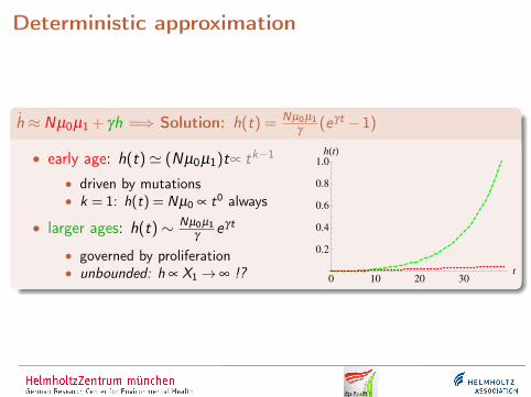
Deterministic approximation

h ≈ Nµ0µ1 + γh =⇒ Solution: h(t) = Nµ0µ1γ

(eγt −1)

• early age: h(t)' (Nµ0µ1)t∝ tk−1

• driven by mutations• k = 1: h(t) = Nµ0 ∝ t0 always

• larger ages: h(t)∼ Nµ0µ1γ

eγt

• governed by proliferation• unbounded: h ∝ X1→ ∞ !?

0 10 20 30t

0.2

0.4

0.6

0.8

1.0

hHtL

l

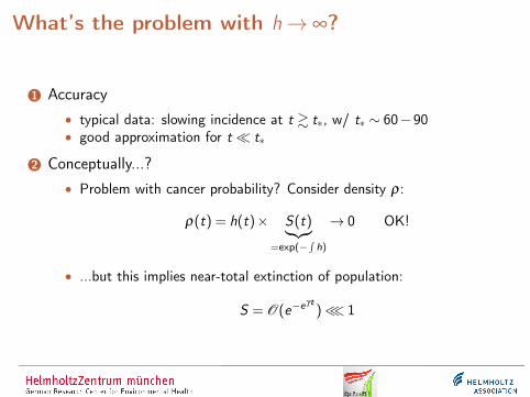
What’s the problem with h→ ∞?

1 Accuracy• typical data: slowing incidence at t & t∗, w/ t∗ ∼ 60−90• good approximation for t� t∗

2 Conceptually...?• Problem with cancer probability? Consider density ρ:

ρ(t) = h(t)× S(t)︸︷︷︸=exp(−

∫h)

→ 0 OK!

• ...but this implies near-total extinction of population:

S = O(e−eγt)≪ 1

l

Can we fix it?

1 Go beyond deterministic approximation h 6= µ1X1 Stochastic model (Sec. 2)

2 Within deterministic model? Start from

h(t) = µ1(t)X1(t); X1 = Nµ0 + γX1

Phenomenological modifications:• Compensate X1 ∼ eγt? Age-dependent µ1(t)∼ e−γt (as t→ ∞)

• Keep X1 bounded? X1!

= 0• Age-dependent γ(t), Nµ0(t)...?• ad-hoc cell-cell interaction term: X1 = Nµ0 + γX1−εX 2

1[Sachs, Rad. Research 164 (2005)]

l




l

Stochastic process

• So far: “Sharp” # of cells Xi (t)

• But cancer evolution is stochastic process:Xi (t) are random, w/ probability

Prob{X1(t) = x1, . . . ,Xk(t) = xk}=: Px1...xk (t)≡ Px(t)

Goal• Find Px(t) with initial condition Px(0) = δx ,0 (healthy cells only)• More precisely, we want to model time evolution

P(t0) 7→ P(t)

l

Markov process

• Markov’s condition: “Short-memory” time evolution,i.e., {Px(t)} completely determines Px(t + ∆t)

• leads to Chapman-Kolmogorov eq.

Px(t + ∆t) = ∑x ′Px ′(t)px ′→x

• Transition probabilities• normalized: ∑x px ′→x = 1• completely define the time evolution (i.e., parametrize our model!)

l

Markov processContinuous-time process

Px(t + ∆t) = ∑x ′(6=x)

Px ′(t)px ′→x +Px(t)

(1− ∑

x ′(6=x)

px→x ′

)= Px(t) + ∑

x ′( 6=x)

(Px ′(t)px ′→x −Px(t)px→x ′)

Master equation• Take ∆t→ 0, assuming px ′→x( 6=x ′) ' Ax ′,x∆t:

ddt

Px(t) = ∑x ′

(Px ′(t)Ax ′,x −Px(t)Ax ,x ′

)• Formal solution: P(t)≡A P(t) =⇒ P(t) = eA tP(0)

l




l

1-stage (Poisson) process

• States: x ≡ (x1) – #cells in stage 1• Assume only 1 transition (from “healthy” → “malignant”)

px ′→x = Nµ0∆t if x ′ = x−1

Px(t + ∆t) = Px−1(t)Nµ0∆t +Px(t)(1−Nµ0∆t)

• Transitions between states:

(x1 = 0)µ0−→ (1)

µ0−→ (2)µ0−→ ·· ·

continuous transfer from (x1 = 0) toward (x1→ ∞)

l

1-stage process: Master equation

Px(t) = Nµ0

Px−1(t)︸︷︷︸transfer from x−1→x

− Px(t)︸︷︷︸transfer x→x+1

; Px(0) = δx ,0

Solve:

Px=0 =−Nµ0P0 ⇒ P0(t) = e−Nµ0t

P1 = Nµ0(P0−P1) ⇒ P1(t) = e−Nµ0tNµ0t...

...

l

Solution: Poisson distribution

Px(t) = e−Nµ0t (Nµ0t)x

x!

• E (X1)≡ X1(t) = Nµ0t – probability “travels” w/ speed Nµ0

• Var(X1)≡∆X 21 = Nµ0t – spreads out

• Steady state as t→ ∞? Px(t) = Nµ0 [Px−1(t)−Px(t)]?= 0

0 2 4 6 8 10x

0.2

0.4

0.6

0.8

1.0

PHx;tL

l

A toy model

Imagine the #cells, x , were continuous: Px(t) =: P(x ; t)

P(x ; t) =−Nµ0 [P(x ; t)−P(x−1; t)]→−Nµ0∂

∂xP(x ; t)

Solution: Any “traveling wave” with P(x ; t) = f (x−Nµ0t)

• Proof: ∂t f (x−Nµ0t) = f ′(x−Nµ0t)︸︷︷︸=∂x f

×[−Nµ0]

• Gives “central” dynamics, but no diffusion

l

Back to “deterministic” model

So far, solved whole problem, Px(t)What is specific dynamics of mean cell #, X (t)?

ddt

X (t) = ∑xx Px(t)

= ∑xx Nµ0 (Px−1−Px)

= Nµ0(X +1−X

)= Nµ0

∴ Heuristic model in Sec. 1 ⇐⇒ Exact dynamics of X (t)

l

Link to risk model

What is the hazard / survival probability for this model?

S(t) = Prob(Tcancer > t) =?

Simplest model: Interpret person as healthy:⇔ X1(t) = 0

S(t) = Prob{X1(t) = 0}= P0(t)

• Survival: S(t) = e−Nµ0t

• Hazard: h(t) =− ddt lnS(t) = +Nµ0

• Same as deterministic model!• Age-independence not realistic for cancer data/biology – let’s move on!

l




l

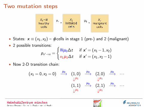
Two mutation steps

• States: x ≡ (x1,x2) – #cells in stage 1 (pre-) and 2 (malignant)• 2 possible transitions:

px ′→x =

{Nµ0∆t if x ′ = (x1−1,x2)

x1µ1∆t if x ′ = (x1,x2−1)

• Now 2-D transition chain:

(x1 = 0,x2 = 0)µ0−→ (1,0)

µ0−→ (2,0)µ0−→ ·· ·

↓µ1 ↓µ1

(1,1)µ0−→ (2,1)

µ0−→ ·· ·↓µ1 ↓µ1

l

2-stage process: Master equation

Px1x2(t) = Nµ0 (Px1−1,x2(t)−Px1,x2(t))

+ x1µ1 (Px1,x2−1(t)−Px1,x2(t))

If we are only interested in the hazard, h =−S/S , with

S(t) = Prob{X2(t) = 0}= ∑x1

Px1,0

then we only need the x2 = 0 entries:

Px1,0(t) = Nµ0 [Px1−1,0(t)−Px1,0(t)]− x1µ1Px1,0(t)

Same as 1-stage process, but w/ loss term for high #1-cells (1→2)

l

Hazard

S = ∑x1

Px1,0 =−µ1 ∑x1

x1Px1,0

h =− SS

= +µ1 ∑x1

x1Px1,0

∑x Px ,0= µ1E (X1|X2 = 0)

• Looks like deterministic approximation,but w/ mean X1|0 conditional on X2 = 0!

• Relevant probability distribution for X1:Px1|0 ≡ Px1,0/∑x Px ,0 (normalized)

l

Back to hazard

Since h = µ1X1|0, all we need is effective equation for X1|0:

ddt

X1|0 = ∑x1

x1[Nµ0

(Px1−1|0−Px1|0

)−(x1− X1|0

)µ1Px1|0

]= Nµ0

(X1 +1−X1

)|0−

(X 2

1|0− X 21|0

)µ1

ddt

X1|0 = Nµ0−∆X 21|0µ1

• “Deterministic” term (from 1st step) – describes mean X1

• “Stochastic” fluctuation term (2nd step)• leads to steady state!• similar effect as phenomenological term inhibiting cell growth (Sec. 1)

l

Hazard: Constant parameters

• For const. parameters: Px1|0 Poissonian ⇒ ∆X 21|0 = X1|0

ddt

X1|0 = Nµ0− X1|0µ1

• strong “damping” if many pre-malign cells (likely already malign –discount, since no longer cause new cancer)

• Rewrite in terms of h = X1|0×µ1:

h = µ1(Nµ0−h) h(t) = Nµ0(1− e−µ1t

)

l

Summary so far

Deterministic model

• Exact equations for mean #cells X1 = µ0X0 + γ1X1

• Approximation for hazard: h ≈ µ1X1

• works well for earlier ages: polynomial / exp. growth• growth unbounded!

Stochastic model• Exact hazard: h = µ1E (X1|X2 = 0)≡ µ1X1|0

• X1|0 obeys similar equation as X1:• same deterministic term (more 1-cells due to µ0)• extra fluctuation term (fewer 1-cells due to µ1)

• Equilibrium at older age: Hazard saturates

l




l

2-stage model w/ clonal expansion

• Deterministic model: h = Nµ0µ1 + (α−β )h• Include stochastic term −∆X 2

1|0 (constant parameters):

h = Nµ0µ1 + (α−β −µ1︸︷︷︸=:γ

)h− α

Nµ0h2

• 1st-order term −µ1h (“Poisson contribution ∆X 2 = X ”)• 2nd-order term ∝−αh2 (“high α X1 ↑ increased loss to 2-cells”)

[Moolgavkar (1979-81)]

l

Phases

h

h'deterministic

Nµ0µ1/q

Nµ0µ1

exact

0 20 40 60 80t

0.2

0.4

0.6

0.8

1.0

hHtL

What can we learn from h = Nµ0µ1 + γh− α

Nµ0h2?

• initially: h ' Nµ0µ1 + γh =⇒ h(t)' Nµ0µ1γ

[eγt −1]

• max. growth: h(t∗) = 0 =⇒ h(t)' h(t∗) + h(t∗)(t− t∗)• steady state: h→ 0 =⇒ h(t)→ Nµ0µ1/q

w/ q(q + γ)≡ αµ1; γt∗ ≡ ln γ+qq

l

Effective parameters

h = Nµ0µ1 + γh− α

Nµ0h2

• Scaling invariance only 3 parameters “ identifiable” from h:• Nµ0µ1; γ (deterministic – early age)• αµ1 (stochastic)

• One interpretation:• time scale: t ′ = γt• hazard scale: h′ = hγ/Nµ0µ1

• functional shape: ε ≡ αµ1/γ2 h′ = 1+h′− εh′2

l




l

Multi-stage models

...X0=N

healthy cells

Xk-1

initiatedcells

µ0 μk-1

αk-1

division

βk-1inactivation/differentiation

Xk

malignantcells

X1

initiatedcells

µ1µ1µ1µ1 µk-2

α1

division

β1inactivation/differentiation

k-stage model w/ clonal expansion (k = 2 ⇐⇒ TSCE)• Parameters

• transitions (µ0,...,k−1): k parameters• proliferation (α1...k−1;β1...k−1): 2(k−1) – too many!

• Qualitative behavior?[Little, Int. J. Rad. Biol. 78 (2002)]

l

Example: 3-stage “pre-initiation” model

Analytic solution

h(t) = Nµ0

1−(qe(γ+q)t + (γ +q)e−qt

γ +2q

)−µ1/α

• 4 (out of 5) identifiable parameters: Nµ0, γ , q, plus µ1/α. . .

• Phases: polynomial ∝t2, exponential, linear, saturation to Nµ0

[Luebeck, PNAS 99 (2002); Meza, PNAS 105 (2008)]

l

What can we really learn?

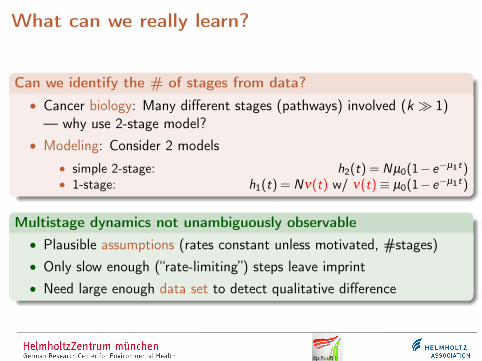
Can we identify the # of stages from data?• Cancer biology: Many different stages (pathways) involved (k � 1)— why use 2-stage model?

• Modeling: Consider 2 models• simple 2-stage: h2(t) = Nµ0(1− e−µ1t)• 1-stage: h1(t) = Nν(t) w/ ν(t)≡ µ0(1− e−µ1t)

Multistage dynamics not unambiguously observable• Plausible assumptions (rates constant unless motivated, #stages)• Only slow enough (“rate-limiting”) steps leave imprint• Need large enough data set to detect qualitative difference

l




l

What about radiation. . .?

• Radiation-induced (epi-)genetic effects• non-repair: apoptosis β ↑• misrepair: additional mutations µi ↑, (α−β ) ↑• . . .

• Toy model to understand effects:

µi (t) = µ(0)i [1+ f (t)] , etc.

f (t) =

{const. t ∈ [t1, t2]

0 else

How could we solve that?

l

µ1(t): Deterministic model

h(t) = µ1(t)X1(t); X1 = Nµ0 + γX1

µ1 = µ(0)1 (1+ f ) =⇒ h = h(0)(1+ f )

• Jump at t1,2: ∆h = ∆µ1X1 — instant effect!• Excess relative risk = f

l

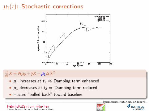
µ1(t): Stochastic corrections

ddtX = Nµ0 + γX −µ1∆X 2

• µ1 increases at t1 ⇒ Damping term enhanced• µ1 decreases at t2 ⇒ Damping term reduced• Hazard “pulled back” toward baseline

[Heidenreich, Risk Anal. 17 (1997]

l

Now for µ0(t):

l

µ0(t)

ddtX = Nµ0 + γX −µ1∆X 2

• Kinks (no jumps): ∆h = µ1×N∆µ0 – extra stage delays effect• Slow return to baseline:Kink at t2 neglible compared to accumulated clonal growth

l

Excercise: α(t)

looking inside mechanistic models of carcinogenesis

Health & Medicine

t t time step t

agedependent t

1tx1t x1

stages x1

n0 x1 x2

deterministic model

x0 x1 xk dxk dt

1x1 stochastic model