Institut C.D. HOWE Institute

commentaryNO. 395

Long-Term Returns: A Reality Check for Pension Funds and Retirement Savings

Pension fund managers and retirement savers could face lower-than-assumed investment returns over the long term using realistic projections. The implications

would be bigger pension liabilities for some defined-benefit pension plans, and a need to save more and work longer for individual savers, if they are

to avoid a larger-than-expected drop in their retirement lifestyles.

Richard Guay and Laurence Allaire Jean

$12.00isbn 978-0-88806-916-0issn 0824-8001 (print);issn 1703-0765 (online)

Essential Policy Intelligence | Conseils indispensablessur les

polit

ique

s

INST

ITU

TC.D. HOWE

INST

ITU

TE

Finn PoschmannVice-President, Research

Commentary No. 395December 2013Pension Policy

C.D. Howe Institute publications undergo rigorous external review by academics and independent experts drawn from the public and private sectors.

The Institute’s peer review process ensures the quality, integrity and objectivity of its policy research. The Institute will not publish any study that, in its view, fails to meet the standards of the review process. The Institute requires that its authors publicly disclose any actual or potential conflicts of interest of which they are aware.

In its mission to educate and foster debate on essential public policy issues, the C.D. Howe Institute provides nonpartisan policy advice to interested parties on a non-exclusive basis. The Institute will not endorse any political party, elected official, candidate for elected office, or interest group.

As a registered Canadian charity, the C.D. Howe Institute as a matter of course accepts donations from individuals, private and public organizations, charitable foundations and others, by way of general and project support. The Institute will not accept any donation that stipulates a predetermined result or policy stance or otherwise inhibits its independence, or that of its staff and authors, in pursuing scholarly activities or disseminating research results.

The Institute’s Commitment to Quality

About The Authors

Richard Guay is a Professor of Finance, UQAM and Fellow, CIRANO.

Laurence Allaire Jean is former Project Director, CIRANO Finance Group.

The Study In Brief

Expectations for investment returns play an important role in establishing business capital cost and capital structure, as well as influencing individual savings behaviour, risk-taking, and long-term funding of institutional obligations such as pensions.

Proper and realistic forecasting makes for better long-term investment decisions improving retirement planning. In this Commentary, we demonstrate why pension plan administrators and individual savers should avoid using historical rates of returns to forecast future returns, and provide our own forecast for long-term investment returns on a balanced portfolio of bonds and stocks using current and prospective market information.

Our empirical analysis of Canadian data provides substantial evidence that forecasts based on past performance should not form a basis for decision-making, as they consistently point in the wrong direction. The history of stock and bond markets is punctuated with extreme situations – such as the recent global financial crisis – that make drawing on the outcome of these events inappropriate as a predictor of future performance. Thus, relying on historical performance to inform long-run return forecasts in pricing future pension liabilities is almost certain to be misleading.

Prospectively, using information available as of February 2013, we predict long-term returns in the neighbourhood of 2.5 percent (0.5 percent real) on long-term bonds and of 6.9 percent (4.8 percent real) on stocks. For a balanced portfolio (50/50 split), we therefore expect a real return of 2.7 percent for the next decade.

To incorporate potential risks to this scenario, we have performed a series of long-term simulations that give a sense of varied possible outcomes. We found significant downside risks. There is a 25 percent probability that portfolio returns will be lower than forecasted by more than one percentage point on a 30-year horizon, and lower by more than 2 percentage points on a 10-year horizon.

Finally, we draw implications for pension funds and individual savers. The use of more realistic investment return expectations would reveal bigger pension liability for some defined-benefit pension plans. They also mean individuals should save more for their retirement to avoid a larger-than-expected drop in their retirement lifestyles.

C.D. Howe Institute Commentary© is a periodic analysis of, and commentary on, current public policy issues. Michael Benedict and James Fleming edited the manuscript; Yang Zhao prepared it for publication. As with all Institute publications, the views expressed here are those of the authors and do not necessarily reflect the opinions of the Institute’s members or Board of Directors. Quotation with appropriate credit is permissible.

To order this publication please contact: the C.D. Howe Institute, 67 Yonge St., Suite 300, Toronto, Ontario M5E 1J8. The full text of this publication is also available on the Institute’s website at www.cdhowe.org.

2

Furthermore, for managers of many large defined-benefit (DB) pension plans, these expectations impact the valuation of liabilities – the present value of promised and future obligations – to determine the appropriate funding ratios to maintain plan viability. It is, therefore, imperative to properly forecast these returns (and, consequently, discount rates) to better reflect the current state of a fund’s obligations and a pension plan’s real annual costs. More generally, proper and realistic forecasting makes for better long-term investment decisions, improving retirement planning.

Plan administrators should avoid using historical returns to forecast future returns. The history of stock and bond markets is punctuated with extreme situations – such as the recent global financial crisis –that make drawing on the outcome of these events inappropriate as a predictor of future performance. This is true for any time horizons even up to 100 years. It is unlikely that the future will bring similar historical events.

Current bond yields are tightly linked to a generalized drop in interest rates over the last few decades. In recent years, yields on long-term government bonds were in the 2 to 3 percent range, compared to yields hovering around 5 percent a decade ago, and 10 percent two decades ago. The analysis developed in this paper shows that such

high historical returns are unlikely to be repeated in the foreseeable future.

Current monetary policies across industrialized countries are also contributing to these historically very low interest rates. Should we conclude that interest rates will climb back to their historical average after a full global economic recovery? For various reasons, we do not see this scenario as plausible.

Monetary policy’s primary impact is on short-term rates, which are commonly now less than 1 percent – a level below inflation. While we can reasonably expect short-term rates to increase to more “normal” levels when central banks start pulling back their extraordinary monetary stimulus, the story is different for long-term bonds. A number of factors – an aging population, many pension funds reaching maturity, as well as stricter financial sector regulations – are combining to create increased demand for long-term bonds, likely keeping their returns at very low levels.

Furthermore, as Beaudry and Bergevin (2013) point out, the new “normal” long-term rate will likely be lower than its historical average. The most important long-term rate factor, they say, will be a rise in savings from emerging countries like China translating into increased demand for safe bonds.

The authors would like to thank Alexandre Laurin and members of C.D. Howe Institute’s Pension Policy Council for their insights and comments on earlier drafts of this paper, as well as their colleagues at CIRANO. Responsibility for the views expressed in this Commentary and for any remaining errors rests with the authors.

Predicted rates of return for stocks and bonds play a central role in establishing an organization’s capital cost, capital structure, as well as its investment and portfolio decisions. For individuals, forecasted returns especially influence savings behaviour and investment decisions.

3 Commentary 395

For stock markets, recent volatility makes forecasts even more precarious. Analysis of historical data shows that at year-end 2008, going as far back as even a decade, most exchanges have experienced negative returns.1

What is to be expected for the next 10 years? We are convinced that relying on historical returns for forecasts is inappropriate. Instead, we formulate long-term predictions using only current and prospective information.

In the first section, we outline our equity-return projections based on current dividend yields as well as leading financial analysts’ economic growth predictions. Our forecasts for long-term stock market returns, therefore, combine current yields, current prices, along with prospective economic growth projections.

We also consider the impact of demographics. For the next few decades, the impact of an aging population will likely correspond to a lower growth rate in developed countries, which puts a downward pressure on the equity premium. This might be accentuated by a sale of equity following a reduction of risk tolerance. However, beyond a forecasting horizon of 30 years, the effect might be ambiguous because reduced risk tolerance would necessitate compensation through higher equity premiums.

The forecast approach we favour for long-term government bonds is based on current yields to maturity. As a result, we derive forecasts that are substantially below those rooted in previous decades’ returns.

Prospectively, we predict long-term returns in the neighbourhood of 2.5 percent (0.5 percent real) on long-term bonds and of 6.9 percent (4.8 percent real) on stocks. For a balanced portfolio (50-50), we

therefore expect a real return of 2.7 percent for the next decade.

Applying such low-return projections when making portfolio and saving decisions has serious implications, especially for an individual who needs to purchase an annuity. A lower discount rate would increase DB pension plans’ liability valuations and also lead to a substantial increase in their annual servicing costs.2

This Commentary is organized in two main sections. The first section is a quantitative analysis of forecasting approaches, where a forward-looking approach is chosen to provide forecasts based on the current market environment. The next section provides implications for retirement savings and pension funds, as well as a broader policy discussion. A conclusion follows that includes other perspectives.

Backward- versus Forward-Looking Forecasting: Approaches and Findings

The cornerstone of our empirical analysis is the substantial evidence that forecasts based on past performance should not form a basis for decision-making, as they consistently point in the wrong direction. Thus, relying on historical performance-based actuarial assumptions for long-run return forecasts in pricing a pension fund’s liabilities are almost certain to be misleading.

This section briefly introduces standard forecasting approaches found in the financial literature, testing them with Canadian data. Then, we introduce our own forecasts based on the current environment. The section concludes with a risk analysis that aims at illustrating various statistical issues, most notably the distribution around forecasts.

1 This decline holds for the US S&P 500 Composite Index and for the MSCI World Index, while the S&P/TSX Composite Index showed positive returns.

2 We observe various funding levels across pension systems – pay-as-you-go for OAS/GIS, a partially funded system for CPP/QPP or a fully funded employer-sponsored plan. This Commentary focuses on the fully funded approach.

4

Elements from the Literature

The literature that has been consulted as background to this paper’s quantitative analysis varies from the more technical and theoretical to the more applied and intuitive.

First, Dimson, Marsh and Staunton (2013) present Canadian historical equity premiums for three time periods, 1900-2012, 1963-2012 and 2000-2012, that are, respectively, 3.4 percent, 1.0 percent and -3.2 percent. In attempting to forecast future returns, these results show how an extrapolation from historical returns could be misleading, since results are very sensitive to the time horizon.

Focusing on the Equity Risk Premium (ERP), Damodaran (2013) measures various ERP estimates. Results show that a current-implied premium approach (based on current equity value and a discounted future cash flow model) easily outperformed a backward-looking, historical-premium forecast. Campbell and Shiller (1988) argue for the current dividend-yield method plus a predicted growth rate as a simple forecasting tool for future returns. The same authors propose other measures, such as the price-to-earnings ratio (P/E) with some historical averaging at the earnings level, to provide some smoothing of forecasts – more precisely, comparing current price to a 10-year average of inflation-adjusted earnings. Leading US economist Jeremy Siegel has also criticized this latest method (the cyclically adjusted price-earnings ratio, or CAPE) for its use of historical data on the grounds that forecasts should be strictly forward looking.3

Robert Arnott, also focusing on risk premium, demonstrates the inaccuracies in using historical figures to forecast long-run returns and determine

a reliable “sustainable equity risk premium.” In Arnott and Ryan (2001), the authors examine a 74-year period, adjusting the measured 5.1 percent risk premium by deducting elements that came from unique historical events that can no longer be repeated. Examples of events that boosted the equity risk premium are: an unprecedented tripling in valuation measured by the P/E ratio; a drop in dividend yield, mainly through important stock buybacks; and relatively higher economic growth in the past compared to projections, in a context where real dividend growth is highly linked to economic growth.

In a nutshell, the 20th century’s financial history contains events that are deemed unique and non-replicable, and should not be a basis for enthusiasm in future long-term returns. Arnott (2011) reconfirmed these findings, also pointing out the problem of survivorship bias in which historical return metrics only apply to still-existing companies, indices and even stock markets themselves, writing, “Our own stock market history is but a single sample of a large and unknowable population of potential outcomes.”

Furthermore, he summarizes his view of relevant forecast tools in Arnott and Bernstein (2002) (with our emphasis):

Few observers have noticed that much of the difference between stock dividend yields and the real returns on stocks can be traced directly to the upward revaluation of stocks since 1982. The historical data are muddied by this change in valuation levels – which is why we find the current fashion of forecasting the future by extrapolating the past to be so alarming. The earnings yield is a better estimate of future real stock returns than any extrapolation of the past. And the dividend yield

3 See “Robert Shiller versus Jeremy Siegel Debate: Are Stocks Overvalued?” http://saxangle.com/2011/04/robert-shiller-versus-jermy-siegel-debate-are-stocks-overvalued/ Accessed Nov. 25, 2013.

5 Commentary 395

plus a small premium for real dividend growth is even better, because in the absence of changes in valuation levels, the earnings yield systematically overstates future real stock returns.

Therefore, similar to the aforementioned authors, our analysis of Canadian data contrasts backward-looking based forecasts with forward-looking ones, in order to assess their respective predictive power.

Results for the Canadian Financial Market Data

To evaluate various forecasting methods, we compare hypothetical 10-year predictions that could have been made in the past to the actual return over that decade. For instance, we simulate a 10-year return prediction that could have been made in 1993 based on then-available information and compare it with actual returns between 1993 and 2003. Accordingly, since we follow a 10-year forecast structure, the last forecasting point must be 2003, which uses data up to 2013 for realized return comparisons.4

The Stock Market

The first series of tests is performed on the main Canadian stock exchange index, the S&P TSX Composite Index, with monthly data for 50 years ranging from 1963 to 2013. Two forecast methods are examined: one based on historical data and another that is forward-looking based on the dividend yield (DY) at the time and prospective economic growth. The historical approach uses the

previous 10-year average return based on the total return index. The forward-looking approach uses the current DY5 and adds the most recent expert GDP forecasts to represent the future growth rate of dividends.6

t t tLongTermStock Return Forecast DY g= +

where DYt represents the dividend yield at time t and tg represents the expert forecast for long-term economic growth.

Table 1 presents comparative results of the two approaches, historical and forward-looking.

We measure predictability by comparing each forecast to the actual 10-year return. The results are unambiguous. Whereas the DY approach generates a 55 percent correlation between prediction and realization, the historical approach generates a negative correlation of 63 percent (Table 1). Furthermore, the volatility of the prediction error, as measured by the standard error in our sample, decreases from 6 percent to 4 percent, which means the precision of forecasts increases by switching from the historical approach to the forward-looking approach (Table 1). Similar correlation results for 1960-2012 can be found in Damodaran (2013).

Figure 1 clearly shows the poor predictive power of using historical returns. On the other hand, the forward-looking approach, DY combined with nominal GDP growth, provides a more reliable prediction (bottom part of Figure 1), as the slope is positive and prediction error is reduced. Each scatter plot reports in its title the

4 It might be preferable to back-test, using horizons such as 50 years or more. However, for practical reasons related to data availability, our back-testing analysis focuses on a 10-year horizon.

5 Other models exist and could be considered (See Davis, Aliaga-Diaz and Thomas). However, the focus of this Commentary is to show that simple forward-looking methodologies do improve substantially the forecasts when compared to a historical approach.

6 For the purpose of back-testing with the available data, we used latest measured yearly GDP growth.

6

correlation estimate (ρ), the slope of a univariate linear regression7 and the F-statistic of the same regression.

The Long-Term Bond Market

Similar comparisons can be made for the long-term bond market. Again, we use the 10-year historical average return as our backward-looking approach and compare it to a simple forward-looking measure: the yield to maturity (YTM).

Long Term Bond Return Forecastt = YTMt

where YTMt is the bond’s yield to maturity at time t.The data come from the Canadian long-term

government bond index (10-year +) and are very similar to the DEX Long Term Bond Index (10-year +). Using monthly data from 1984 to 2013, we compared each forecasting measure to the realized return on those bonds over the following 10 years. Table 2 presents the correlations and the volatility of the forecasting error for two forecasting models.

Results from Table 2 are similar to those of the stock market computations above, with both negative historical and positive forward-looking correlations as well as smaller prediction-error volatility for the forward-looking measure when compared to the historical, backward-looking approach. Also similar to Figure 1, a scatter plot chart for bonds clearly shows the negative correlation of the historical approach, whereas using the redemption yield as a forward-looking predictor correlates much more closely (and in the right direction) to the future realized returns it is trying to predict.

The following charts graphically present this empirical measure (Figure 2). Each scatter plot includes the correlation estimate (ρ), the slope of a univariate linear regression and the F-statistic associated to the linear regression.

Current Forward-Looking Forecasts

The literature and quantitative results above provide justification for applying forward-looking measures

7 The slope (b) of the regression is RRt,t+10 = a + b∙FMt where FM is the forecasting model value at time t and RRt,t+10 is the realized return for the next 10 years (from time t to t+10).

Table 1: Predictability of Backward- versus Forward-Looking Forecasts (Stock Market)

Historical Approach Forward-Looking Approach percentCorrelation with Realized Returns -63 55Volatility of Prediction Error 6.0 4.2

Sources: S&P/TSX Composite Total Return Index and Dividend Yield, 1963-2013 (596 monthly observations). Authors’ calculations on a 10-year horizon (356 10-year forecasts).

7 Commentary 395

Source: S&P/TSX Composite Total Return Index and Dividend Yield, 1963-2013 (596 monthly observations).Authors’ calculations on a 10-year horizon (356 10-year forecasts).

Figure 1: Comparing the Predictive Power of Forecasts versus Realized Returns on Stocks

0

5

10

15

20

25

0 5 10 15 20 25

Forecast (percent)

TSX: Historical Approach vs. Realized Returns

ρ = -63%, slope = -0.57, F-test = 233

0

5

10

15

20

25

0 5 10 15 20 25

Forecast (percent)

TSX: Forward-Looking Approach vs. Realized Returns

Rea

lized

Ret

urns

(per

cent

)R

ealiz

ed R

etur

ns (p

erce

nt)

ρ = 55%, slope = 0.35, F-test = 157

8

in our own forecasts. As we will see, the forecast numbers thus computed caution against developing policies based on optimistic long-term returns.

The following table presents our forecasts on a 10-year horizon, as of February 2013, based on a forward-looking method, and is followed by more specific information.8 (Interest rates and other factors have changed during the course of 2013, so using the most current information would lead to slightly different results.9)

On the stock market side, our February 2013 sample point reflects a 3.02 percent DY. When added to the Parliamentary Budgetary Officer 2012 real GDP long-run forecast of 1.8 percent,10 we predict an average 4.82 percent real annual return over the next 10 years. Using a 2 percent inflation level (the Bank of Canada target), our forecast for

nominal returns on Canadian stocks is 6.92 percent over the next 10 years.11

On the long-term bond market side, our latest (February 2013) sample point has a 2.5 percent YTM, which represents our forecast in nominal terms. Using the same inflation forecast, this implies a Canadian long-term bond market real returns forecast of 0.49 percent (= 1.025/1.02 -1) over the next 10 years.

For our portfolio forecast, we assume an asset allocation of 50 percent equities and 50 percent bonds, which corresponds to the average asset allocation of many Canadian pension plans.12 Therefore, we project a real return of 2.66 percent on a balanced portfolio over a 10-year horizon, and a corresponding 4.71 percent nominal return.

8 These forecasts do not include investment expenses (ranging from 0.3 percent for a large pension plan to more than 1 percent for small pension plans or individual savers). This leaves room for return enhancement in some funds (e.g., 60/40 weights instead of 50/50) although at a higher risk, which would lead to the same return forecast after fees.

9 Due to higher bond yields, slightly lower long-term GDP growth projection, and lower dividend yield, our forecast for the portfolio as of September 30, 2013, would be 3.17% real, and 5.23% nominal.

10 See: Parliamentary Budget Officer – Fiscal Sustainability Report 2012. Other authorities making similar long-term economic forecasts include the Conference Board of Canada, the Department of Finance, Canadian commercial banks and the International Monetary Fund.

11 Using the following compounding formula: 6.92% = (1 + 4.82%)*(1 + 2%) – 1.12 The Towers Watson 2012 survey of DB pension funds reports an average asset allocation of about 50-50 for Canadian

pension plans (Towers Watson 2012a).

Table 2: Predictive Power of Backward- versus Forward-Looking Forecasts (Bond Market)

Historical Approach Forward-Looking Approach percentCorrelation with Realized Returns -52 85Volatility of Prediction Error 2.0 0.6

Sources: Datastream Canadian Government Index / DEX Long Term Bond Index, 1984-2013 (338 monthly observations). Authors’ calculations on a 10-year horizon (218 10-year forecasts).

9 Commentary 395

Sources: Datastream Canadian Government Index / DEX Long Term Bond Index, 1984-2013 (338 monthly observations). Authors’ calculations on a 10-year horizon (218 10-year forecasts).

Figure 2: Comparing the Predictive Power of Forecasts versus Realized Returns on Bonds

5

6

7

8

9

10

11

12

13

9 10 11 12 13 14 15

DEX: Historical Approach vs. Realized Returnsρ = -52%, slope = -0.56, F-test = 34.8

5

6

7

8

9

10

11

12

13

4 5 6 7 8 9 10

DEX: Forward-Looking Approach vs. Realized Returns

ρ = 85%, slope = 0.95, F-test = 256

Rea

lized

Ret

urns

(per

cent

)R

ealiz

ed R

etur

ns (p

erce

nt)

Forecast (percent)

Forecast (percent)

1 0

One could argue against relying on such low-level predicted returns by invoking “mean-reversion,” a theory often discussed in the literature suggesting that rates of returns tend to revert back to their long-term average. However, we believe this scenario to be implausible because of demographic factors, the maturity of pension plans and regulatory pressure pushing financial institutions (banks, insurance) away from risky to lower-risk assets such as government bonds. Also, Beaudry and Bergevin (2013) claim that today’s highly integrated world bond market and the long-term “rise of China and the concomitant rise in its level of savings by households” will put pressure to keep interest rates on long-term government bonds at low levels.

Risk Analysis

While we will work with the Table 3 forecasts for the rest of this Commentary, we pause here to note that some components were left out of the above calculations for simplicity’s sake.

The main excluded factor is risk. Risk is the dispersion of return outcomes for each asset class and for the portfolio as a whole. This dispersion has two main implications: first, different return realizations may cause the return for the next decade to be below our average forecast returns (obviously, it could also be above, but we are

concerned with downside); second, as we mix different assets with different risk profiles, the non-perfect correlation between them will have a beneficial effect on the volatility of the portfolio by reducing it through the effect of diversification. The latter point is a well-known statistical phenomenon, so we won’t expand on it.

To elaborate on and to measure potential downside risk, we have performed a series of simulations that give a sense of varied possible outcomes. Using models for stocks and bonds (see Appendix), we built a 50-50 portfolio based on the simulated returns for each asset class and incorporating a correlation structure. Simulations for realized returns were performed on various long-term time horizons.

For the 10-year horizon, we have presented the distributional results in Table 4.

A first change from applying downside risk is that stock returns are 5.75 percent on average, lower than the simulation long-term trend of 6.92 percent. The reason is the effect of volatility in percentage returns that creates an asymmetry from adverse shocks. For instance, after a 10 percent drop of the index, say from 100 to 90, a subsequent 10 percent increase has a smaller effect (+ 9 = 90 × 10 percent) than a subsequent 10 percent return after a gain, say from 100 to 110 (+ 11 = 110 × 10 percent).

Table 3: Current 10-Year Forecasts using the Forward-Looking Approach, as of February 2013

Forecast Real Nominal percentStocks 4.82 6.92Long-Term Bonds 0.49 2.5050-50 Portfolio 2.66 4.71

Source: Data from S&P/TSX, Datastream, PBO, Bank of Canada and authors’ calculations.

1 1 Commentary 395

By incorporating risk, we expect returns to converge

to 21

2µ σ− , where μ is the long-term mean return

and σ2 is its variance.A second interesting result of this simulation

is the lower average realized return on bonds at 1.8 percent, below the forecasted return of 2.5 percent. This is because our model allows a long-term convergence of 3.8 percent for the bond yields, which is above current yields.13 A general (yet modest) increase in interest rates generates a loss in capital for the bond that reduces the total returns. On longer horizons, like 30 years or more, this effect is almost nonexistent as the realized returns gradually converge to its long term trend.

A third and important result is that the overall simulated portfolio performance has an average realized return of 4.18 percent, which is below our basic forecast of 4.7 percent in Table 3.

Turning now to the quantiles for this returns distribution, we focus on the 25th and 10th percentiles. For the portfolio, we see that there is a 25 percent probability of experiencing returns equal

or lower than 2.28 percent. Similarly, investors have a 10 percent probability of experiencing returns equal to or below 0.55 percent for the next decade. This downside risk is central in retirement planning as it could force plan members or savers to contribute more to the plan or to substantially delay retirement in order to achieve a given retirement income objective.

It is also interesting to perform simulations on longer time horizons. We now present results for a 30-year time horizon.

At the portfolio level, the main differences between the 10-year and 30-year horizons are higher overall returns (closer to our basic forecast of 4.7 percent) and tighter distribution around the mean, as illustrated by lower-end quantiles posting a better performance. Higher overall returns chiefly arise as a consequence of higher returns on bonds, due to their long-term convergence toward a higher level (albeit very slowly). Furthermore, and this is also true for the tighter distribution phenomenon, the correlation structure and its beneficial

Table 4: Simulation Results for a 10-Year Horizon

Geometric Average Median Q25 Q10 percentStock Returns 5.75 5.80 1.96 -1.41Bond Returns 1.80 1.81 1.11 0.40Portfolio Returns 4.18 4.20 2.28 0.55

Source: Authors’ calculations. (See Appendix for model assumptions.)

13 We use a very long-term trend to reach the 1.8 percent return, i.e., the 1900-2012 real bond return average reported by Dimson et al. (2013) augmented by the 2 percent inflation target of the Bank of Canada. (See Appendix for an explanation.)

1 2

diversification effect is accentuated over time. The diversification across time periods also kicks in. Still, despite relatively better returns on this horizon, these levels are both below most actuarial assumption levels (as presented in the next section), as well as being subject to important downside risks, as measured by values of the 25th and 10th quantiles.

Implications for Retirement Savings and Pension Funds

This section puts our forecasts in perspective with a quick description of the current actuarial environment, in terms of assumptions prevailing in the Canadian pension fund industry. Then, we measure implications for both individual savers (equivalently, members of a defined-contribution plan) and for defined-benefit pension plans. The section concludes with policy implications.

For simplicity and ease of interpretation, we rely on our initial portfolio forecasts (Table 3). Yet, we incorporate the observed dispersion from the simulation by adding a scenario with a reduction in returns somehow reflecting a lower ranking for a pension fund (e.g., last quartile) and the management fees faced by an individual saver. Even if those scenarios could be more severe, we

will consider a drop of one percentage point from average returns to show the sensitivity of results.

Survey of Actuarial Assumptions in Canada’s Pension Fund Industry

Compared to our forecasts, current Canadian actuarial assumptions tend to be optimistic. For example, in its 2012 edition of the Global Survey of Accounting Assumptions for Defined Benefit Plans, Towers Watson reports an average projected Canadian plan return of 6.4 percent (Towers Watson 2012a). However, Dimson et al. (2013) describe this level, in their Credit Suisse report as: “optimistic. For Canada (…), the implied real equity return is greatly above the level we deem plausible.”

To better illustrate the environment of return assumptions, we examined documentation by the largest Canadian pension funds and observed a projected nominal annual return range from 5.3 percent to 6.9 percent, and from 3.0 percent to 4.5 percent for projected real annual returns. The 6.4 percent average projection above falls nicely in this range. In real terms, accounting for the Bank of Canada 2 percent target inflation rate, this translates in average pension funds real return expectation of 4.3 percent – a level above our

Table 5: Simulation Results for a 30-Year Horizon

Geometric Average Median Q25 Q10 percentStock Returns 5.55 5.54 3.42 1.54Bond Returns 3.09 3.09 2.74 2.42Portfolio Returns 4.77 4.74 3.67 2.75

Source: Authors’ calculations. (See Appendix for model assumptions.)

1 3 Commentary 395

14 Implicit pension fund real return = 4.31% = (1+6.4%)/(1+2%). That is the reported 6.4 percent from the Towers Watson survey on Canadian pension funds, with a two-percentage-point inflation adjustment (Towers Watson 2012a).

15 See Towers Watson (2012b).16 As far as public policy is involved, our view is that the government should promote a basic replacement level (50 percent),

for example through automatic savings. Reaching the “ideal” 70-percent-replacement level remains the individual’s decision and responsibility. See Campbell.

17 Savings rate excludes fiscal/RRSP constraints, which could reduce after-tax returns for some cases when required savings rates exceed RRSP limits.

2.7 percent forecast in Table 3.14 Our lower projected returns have important implications for both individual savers and pension funds.

It should be noted that discount rates do not necessarily correspond to projected returns on assets. For instance, to calculate the funding ratio, some pension funds may use discount rates that are slightly lower than their projected returns to account for adverse deviations. However, for the solvency valuation, which is not the focus of this paper, pension plans typically use current corporate bond rates.

Clearly, optimistic projections could prove problematic. First, such optimism could mislead individuals in their savings behaviour when preparing for retirement. Second, they hide the reality about the scale of accumulated obligations within defined-benefit pension funds as well as their annual costs when projected returns are used as the discount rate.

In meeting the challenge of high costs and deficits of some pension plans, it is essential to acknowledge these realities. Once more realistic assumptions are incorporated, negotiations for adjustments might be required (but will be difficult) in order to reduce costs and deficits to acceptable levels.

On the DC Plans’ and Individual Savers’ Side

Individual savers, as well as members of increasingly popular15 defined-contribution (DC) schemes, are directly facing a new economic reality of low

expected returns. In the early 1990s, real interest rates for Canadian bonds were above 4 percent. Currently, rates are at historically low levels.

One way to measure the impact on the required effort that now must be considered when planning retirement saving decisions is through various scenarios. Using our own software program, we provide such results for two income profiles (Table 6). The first is of someone retiring after reaching a pre-retirement annual income level of $50,000. The second income profile is for a pre-retirement income of $100,000.

Both people start saving today at age 35 and retire at 65. We generate results for income replacement levels of 50 percent, 70 percent and 100 percent at retirement.16 Computations include federal OAS/GIS as well as CPP/QPP. The calculations indicate the saving levels throughout the career (as a proportion of income) required to sustain a given post-retirement income.17

In a lower, more realistic real-return environment of 2.66 percent, the saving effort necessary to achieve the same income replacement is quite higher than under more optimistic expectations (Table 6). For an income of $50,000 or above, the required savings rate is nearly 1.5 times greater than under an optimistic forecast. For example, to reach the popular target of 70 percent income replacement for a $50,000 final income, the necessary savings rate, over 30 years, jumps from 9.6 percent to 14 percent of annual gross salary.

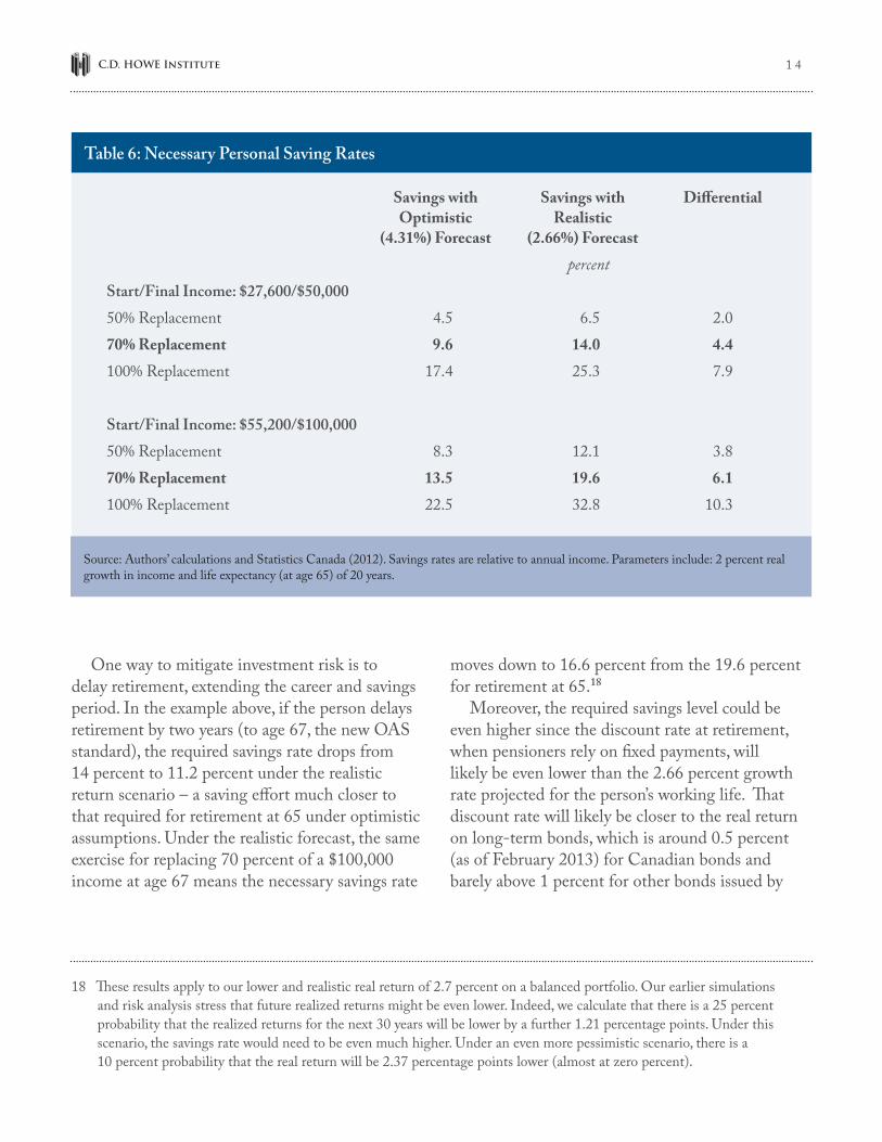
1 4

Table 6: Necessary Personal Saving Rates

Savings with Savings with Differential Optimistic Realistic (4.31%) Forecast (2.66%) Forecast percentStart/Final Income: $27,600/$50,000 50% Replacement 4.5 6.5 2.070% Replacement 9.6 14.0 4.4100% Replacement 17.4 25.3 7.9

Start/Final Income: $55,200/$100,000 50% Replacement 8.3 12.1 3.870% Replacement 13.5 19.6 6.1100% Replacement 22.5 32.8 10.3

Source: Authors’ calculations and Statistics Canada (2012). Savings rates are relative to annual income. Parameters include: 2 percent real growth in income and life expectancy (at age 65) of 20 years.

One way to mitigate investment risk is to delay retirement, extending the career and savings period. In the example above, if the person delays retirement by two years (to age 67, the new OAS standard), the required savings rate drops from 14 percent to 11.2 percent under the realistic return scenario – a saving effort much closer to that required for retirement at 65 under optimistic assumptions. Under the realistic forecast, the same exercise for replacing 70 percent of a $100,000 income at age 67 means the necessary savings rate

moves down to 16.6 percent from the 19.6 percent for retirement at 65.18

Moreover, the required savings level could be even higher since the discount rate at retirement, when pensioners rely on fixed payments, will likely be even lower than the 2.66 percent growth rate projected for the person’s working life. That discount rate will likely be closer to the real return on long-term bonds, which is around 0.5 percent (as of February 2013) for Canadian bonds and barely above 1 percent for other bonds issued by

18 These results apply to our lower and realistic real return of 2.7 percent on a balanced portfolio. Our earlier simulations and risk analysis stress that future realized returns might be even lower. Indeed, we calculate that there is a 25 percent probability that the realized returns for the next 30 years will be lower by a further 1.21 percentage points. Under this scenario, the savings rate would need to be even much higher. Under an even more pessimistic scenario, there is a 10 percent probability that the real return will be 2.37 percentage points lower (almost at zero percent).

1 5 Commentary 395

provincial governments or municipalities. Such fixed-income rates play a crucial role in pricing annuities, which are frequently a major component of retirement income.

There is a third, pessimistic forecast based on negative factors not considered above. To acknowledge these possibilities, we consider a further drop of one percentage point in real returns to reach an even more conservative 1.66 percent growth forecast (Table 7). This drop reflects the real risk of lower realized returns and the costs of investment management (especially in DC plans).

Required savings rates are obviously much higher when one percentage point is removed annually from the returns on savings. For instance, providing

a 70 percent replacement level to an individual earning $50,000 at career end at 65 would require a 17.6 percent savings rate out of annual income compared to 14 percent under the realistic forecast.

Finally, if we consider new mortality tables proposed by the Canadian Institute of Actuaries,19 which increase life expectancy at retirement by more than two years, necessary savings would increase even more. For instance, the $50,000 final income case where the individual aims at a replacement of 70 percent would require saving rates of 10.4 percent, 15.3 percent and 19.4 percent for the optimistic, realistic and pessimistic forecasts, respectively.

Table 7: Necessary Saving Rates (More pessimistic)

Savings with Savings with Differential Optimistic Pessimistic (4.31%) Forecast (1.66%) Forecast percentStart/Final Income: $27,600/$50,000 50% Replacement 4.5 8.1 3.770% Replacement 9.6 17.6 7.9100% Replacement 17.4 31.7 14.3 Start/Final Income: $55,200/$100,000 50% Replacement 8.3 15.1 6.870% Replacement 13.5 24.6 11.1100% Replacement 22.5 41.0 18.5

Source: Authors’ calculations and Statistics Canada (2012). Savings rates are relative to annual income. Parameters include: 2 percent real growth in income and life expectancy (at age 65) of 20.

19 See The Actuary – “Canada’s soaring life expectancy ‘presents DB pension challenge’.”

1 6

On the DB Plans’ Side

As seen above, the average projected rate of returns used to evaluate the actuarial funding ratio for many DB plans is greater than 6 percent. A more realistic 4.7 percent return on a balanced portfolio would – not surprisingly – substantially increase these funds’ liabilities. Such a discount rate adjustment would reveal a higher actuarial funding deficit for many pension plans. Considering discount rates well below current assumptions would, as recently highlighted by the Quebec government’s D’Amours Committee (Quebec 2013), shed some light on the truth about accumulated liabilities as well as true costs for these pension plans.

Evaluating a Pension Plan’s Liabilities

For public-sector plans, lower expected returns on investment leads to discounting accrued and future liabilities at a lower discount rate – and the lower the discount rate, the higher the level of liabilities. Even though some public-sector plans are maturing more quickly than others, which means a lower duration of liabilities, many still have liability durations beyond 15 years. (In finance, duration is a measure of debt sensitivity to the rate used for pricing it.) Here, being conservative and assuming a duration of only 15 years would roughly mean that any one percentage point change in the rates used for pricing the liability would translate into an upward shift of over 15 percent in liability value.

Therefore, if we reduce the pension funds’ discount rate from 6.4 percent to 4.7 percent, it would increase the liabilities by roughly 25 percent (or -1.7 percent × 15) compared to what is currently reported. Moreover, if we follow the D’Amours Committee recommendation to use a discount rate corresponding to a safe bond return when calculating present value of benefits to be paid to pensioners, the pension liability would be much higher.

Let’s consider a realistic but hypothetic situation of a public sector pension plan in which the asset value is 20 percent below current (normalized) actuarial liability. We suppose an asset size of $0.8 billion and a $1 billion liability (with a discount rate of 6.4 percent); in other words, a plan with a 20 percent deficit.

First, it is worth noting that even with a 6.4 percent projected asset return, the deficit for this plan still continues to increase in dollar terms. To keep this deficit constant in dollars, the asset return must be higher. In fact, realized returns on asset must reach 8 percent. This is quite unrealistic in the long run.

$16.4% 8%.$0.8

BB

× =

In short, assets require realized returns to be higher than the discount rate in order to fulfill future obligations when the fund is in deficit. As the equation above demonstrates, an 8 percent return on $0.8 billion generates $64 million annually over a decade, an amount necessary to offset the annual liability cost of $64 million. In practice, absent higher returns or reduced benefits, plans must increase contribution levels to make up the actuarial deficit over time.

Second, assuming a lower and more realistic future rate of return would increase the liability value by about $250 million to reach $1.25 billion, thus widening the deficit since the assets have not changed from their current level. The resulting deficit would then exceed 36 percent instead of the reported 20 percent.

Pension Plan’s Liability as Proper Debt

For a market valuation of future benefits, the discount rate must take into account that those benefits are guaranteed by the sponsor. In this way, for many federal, municipal and university

1 7 Commentary 395

plans, and several provincial government plans, future benefits represent debt.20 Thus, in a market context, the rate of return on long-term bonds of these entities is a better guide to estimate liabilities linked to their pension plans and, more obviously, for the portion of those liabilities that are current pension benefits paid to retirees. To continue with the previous public pension plan example, such an adjustment would push the liability level well above $1.25 billion, which implies a deficit figure well in excess of 40 percent.

Effects on Annual Costs

In their recent work on federal DB pension plans, Robson and Laurin (2012) show the huge annual cost or contribution that is necessary to fund those pension plans in the long run when we use the low return on Canadian bonds that is likely to prevail in the next decade. The annual cost of some federal DB plans exceeds 50 percent of annual wages. It hits 70 percent of annual wages for the DB plan for the Members of Parliament.

Similarly, based on our DC calculations (that is savers facing the same economic environment as funds), a change-in-returns assumption could increase annual costs by 45 percent on the contribution side.

Policy Implications

First, since these liabilities already exist, adjusting to a more appropriate discount rate would allow a more accurate view of current liabilities and their considerable weight on the financial situation of these plans if the situation persists in the future. To achieve sustainability for DB pension plans, it is imperative as a first step to be transparent about

some of their very high costs. Once these costs are revealed, employers (and plan members) can then proceed to perform the adequate adjustments on the cost side as well as on the accumulated deficit side to ensure sustainability.

Further, the true cost of a DB pension plan is not known with certainly until the last benefit payment is made to the last beneficiary. For instance, referring to our earlier simulation results (Tables 4 and 5), there is a significant probability (over 25 percent) of returns being at least one percentage point below our forecast, leading to even higher realized plan costs.

Next, some stakeholders consider unacceptable the reduction of retirement-linked benefits. Before 2000, many plan decision-makers and sponsors approved advantageous ancillary benefits that are still part of the pension benefits world today. However, these modifications occurred in a context where long-term economic perspectives were deemed promising, with stock and bond market returns much higher than what we can expect for the next decade. Nowadays, we are well aware that overly optimistic economic and financial perspectives from before 2000 did not materialize and that returns tanked.

Thus, we believe that the cost linked to these erroneous predictions should be attenuated. Yet, in a spirit of fair risk and cost-sharing between employees and employers, it may be desirable, as proposed by the D’Amours Committee, that any employee benefit concessions be accompanied by a similar effort by employers toward plan deficit reduction. Furthermore, considering that the sponsor currently supports a large proportion of total costs and risks in many public-sector pension schemes, the D’Amours Report suggests that this proportion be reduced.

20 These future benefits are considered to be a debt to be paid to current and future retirees, regardless if paid with accumulated assets or with a sponsor contribution.

1 8

Conclusion

By providing simple and more reliable ways to predict long-term returns on stock and bond markets, this Commentary offers realistic forecasts for a balanced portfolio’s long-term returns for the next decade.

The result is substantially lower than current Canadian pension fund projections. More precisely, we forecast a nominal (real) return of 4.7 percent (2.7 percent) whereas the average pension fund projection is 6.4 percent (4.3 percent).

The analysis has been done within the realm of traditional investment vehicles; publicly tradable stocks and long-term government bonds. Indeed, Towers Watson (2012a) presents survey results for Canadian DB pension funds that are consistent with the 50-50 allocation. Of course, the pension plan could increase the equity allocation to 60 percent or more. This would improve expected returns, but will also introduce more risk that might not be appropriate for many pension plans.

There are ways for pension funds to potentially mitigate, at least to some extent, the effect of a low-return environment of stocks and bonds. This is done by capturing other risk premiums in the managed portfolio. For instance, it is possible to reap a potential risk premium if we move the portfolio to illiquid assets such as real estate, private equity and infrastructure to increase the expected return on the global portfolio. This could be done without increasing the observed volatility of the portfolio returns.

Still, this is not a free lunch as those illiquid assets increase significantly other risk. In particular, it increases the risk (and costs) related to (i) the

selection of an under-performing manager, (ii) the legal risk related to additional and deal-specific contracts enforcements and of course, (iii) the liquidity risk. Thus, increasing the allocation to those illiquid assets may increase expected returns but with a broader definition of risk – not only the observed volatility – it is an open debate if those assets do really provide a better risk-return profile.21

The impacts of an adjustment toward a more realistic discount rate, based on predicted returns, affect both individual savers (or members of a defined-contribution plan) as well as DB pension plans. The latter are required to report liability and manage assets reflecting anticipated future returns. Adjusting DB pension plan liabilities provides a more pessimistic, yet more realistic view of the real costs and funding deficits they are facing.

The use of a more appropriate discount factor would reveal the bigger pension liability of some DB pension plans. Then, it would be more likely that negotiations could take place to reduce their annual costs and accumulated funding deficits to acceptable levels.

Finally, our lower, although more realistic, projected real return on a balanced portfolio might not be low enough. For instance, simulation results indicate there is a 10 percent probability that returns for the next 30 years will be equal or below 2.8 percent (or 0.7 percent real). Under such a scenario, the savings rate and the pension deficit would be huge, and there would be no way to avoid increases in savings and contributions, as well as significant reductions in pension benefits.

21 See Franzoni, Nowak and Phalippou (2012).

1 9 Commentary 395

Appendix: Simulation Models and Methods

The simulation models used in the section on risk analysis are described below.

Stocks

The model for stocks is the simpler one. It assumes a random walk structure, with a drift representing the long-term average, the authors’ forecast.

The equation for the model is:

pt = p

t – 1. (1 + μ + σ. dw

1,t)

where

Pt : The current price level of the index (with P0 = 100)

μ : The drift parameter, the long-term average for returns (6.92%)

σ : The volatility of returns (the historical annual volatility on the TSX from 1956 to 2013, that is 17.19%)

dW1,t : A stochastic shock following a bivariate normal distribution that is correlated to the bond market (the bivariate distribution is N( 0, V), where 0 is a 2×1 vector of zeros)

V : The covariance matrix representing the correlation structure between stocks (TSX) and bonds (DEX). The matrix is 2×2 with diagonal elements being ones and off- diagonals being the correlation ρ.

ρ : The correlation between returns for stocks and bonds (the historical correlation from 1986 to 2013, that is 0.2126).

For each simulation outcome k, a geometric average for returns is computed for any time horizon n in the following way:

,,

0

1.

= − k n

nk n

PR

P

Bonds

The model for bonds is similar to that for stocks, but incorporates additional features. It is very similar to the Cox-Ingersoll-Ross model for interest rates.

Our model first simulates the bond market’s yield to maturity (or interest rate) through the equation:

( )1 1 1 2,σ− − −= + ⋅ − + ⋅ ⋅t t t t tr r a b r r dW

with

0.5 7.0≤ ≤t% r %

and

σ σ= ⋅LT

LT

Fr

where

rt : The current interest rate (with r0 = 2.50%, the latest YTM of our sample, that is from January 2013)

a : The mean-reversion parameter, or speed of reversion (here, it is set at 0.25)

b : The long-term trend, from the historical value of long-term bonds (set at 3.8%, Dimson et al. 2013 reported average at 1.8% real for the period 1900-2012, to which is added two percentage points for inflation)

2 0

σLT : The long-term (LT) historical volatility for yields on Canadian over-10-year bonds (the historical value comes from the period 1985 to 2013, and is 2.65%)

rLT : The long-term (LT) historical value for yields on Canadian over-10-year bonds (the historical value comes from the period 1985 to 2013, and is 6.70%)

F : Adjustment factor to bring yield volatility to a level generating a simulated volatility on bond returns in line with historical levels (F = 1/2.95)

dW2,t : A stochastic shock following a bivariate normal distribution correlated to the stock market (the bivariate distribution is N(0, V), where 0 is a 2×1 vector of zeros)

V : The covariance matrix representing the correlation structure between stocks (TSX) and bonds (DEX). The matrix is 2×2 with diagonal elements being ones and off- diagonals being the correlation ρ.

ρ : The correlation between returns for stocks and bonds (the historical correlation from 1986 to 2013, that is 0.2126).

Assuming a constant duration of 13.67 (the long-term DEX duration as of February 2013), yearly returns are computed based on the fluctuations of the interest rates. From those yearly returns, a geometric average is computed for various time horizons.

With both stock and bond simulation outcomes (5,000 simulations were performed with a maximum horizon of 50 years), a portfolio with constant weights at 50 percent is constructed and its performance measured over various time horizons.

2 1 Commentary 395

References

Arnott, Robert, and Peter Bernstein. 2002. “What Risk Premium is ‘Normal’?” Financial Analysts Journal. Vol. 58, No. 2: 64-85.

Arnott, Robert, and Ronald Ryan. 2001. “The Death of the Risk Premium: Consequences of the 1990s.” Journal of Portfolio Management. Spring.

Arnott, Robert. 2011. “The Biggest Urban Legend in Finance.” Fundamental Index Newsletter. March.

Beaudry, Paul, and Philippe Bergevin. 2013. “The new ‘Normal’ for Interest Rates In Canada: The Implications of Long-Term Shifts in Global Saving and Investment.” E-Brief. Toronto: C.D. Howe Institute. May 29.

Campbell, Bryan, et al. 2011. “Pensions 4-2 au Québec: Vers un nouveau partenariat.” Montreal: CIRANO.

Campbell, John, and Robert Shiller. 1988. “The Dividend-Price Ratio And Expectations Of Future Dividends And Discount Factors.” Review of Financial Studies. v1(3), 195-228.

––––––––––––––. 1998. “Valuation Ratios and the Long-Run Stock Market Outlook.” Journal of Portfolio Management. Vol. 24, No. 22.

Dimson, Elroy, Paul Marsh and Mike Staunton. 2013. Credit Suisse Global Investment Returns Yearbook 2013. Credit Suisse Research Institute.

Damodaran, Aswath. 2013. Equity Risk Premiums (ERP): Determinants, Estimation and Implications – The 2013 Edition. New York University – Stern School of Business.

Davis, Joseph, Roger Aliaga-Diaz, and Charles J. Thomas. 2012. “Forecasting stock returns: What signals matter, and what do they say now?” Valley Forge, Pa. Vanguard Research.

Franzoni, Francesco, Eric Nowak, and Ludovic Phalippou. 2012. “Private Equity Performance and Liquidity Risk.” The Journal of Finance. November 19.

Parliamentary Budget Officer (PBO). 2012. Fiscal Sustainability Report 2012. Ottawa.

Quebec. 2013. Innovating for a Sustainable Retirement System. Report of the Expert Committee on the Future of the Quebec Retirement System. Alban D’Amours chaired the committee.

Robson, William, and Alexandre Laurin. 2012. “Federal Employee Pension Reforms: First Steps – on a Much Longer Journey.” E-Brief. Toronto: C.D. Howe Institute. November 1.

Statistics Canada. 2012. “Life expectancy, at birth and at age 65, by sex and by province and territory.” Ottawa. CANSIM, Table 102-0512.

The Actuary. 2013., “Canada’s soaring life expectancy ‘presents DB pension challenge’.” August 7.

Towers Watson. 2012a. “Global Survey of Accounting Assumptions for Defined Benefit Plans.”

––––––––––––. 2012b. “International Pension Plan survey 2012.” London. November.

Notes:

Notes:

Notes:

Support the InstituteFor more information on supporting the C.D. Howe Institute’s vital policy work, through charitable giving or membership, please go to www.cdhowe.org or call 416-865-1904. Learn more about the Institute’s activities and how to make a donation at the same time. You will receive a tax receipt for your gift.

A Reputation for Independent, Nonpartisan ResearchThe C.D. Howe Institute’s reputation for independent, reasoned and relevant public policy research of the highest quality is its chief asset, and underpins the credibility and effectiveness of its work. Independence and nonpartisanship are core Institute values that inform its approach to research, guide the actions of its professional staff and limit the types of financial contributions that the Institute will accept.

For our full Independence and Nonpartisanship Policy go to www.cdhowe.org.

Recent C.D. Howe Institute Publications

November 2013 Richards, John. Diplomacy, Trade and Aid: Searching for ‘Synergies.’ C.D. Howe Institute Commentary 394.November 2013 Blomqvist, Åke, Boris Kralj, and Jasmin Kantarevic. “Accountability and Access to Medical Care: Lessons from the Use of Capitation Payments in Ontario.” C.D. Howe Institute E-Brief.November 2013 Neill, Christine. What you Don’t Know Can’t Help You: Lessons of Behavioural Economics for Tax-Based Student Aid. C.D. Howe Institute Commentary 393.November 2013 Dachis, Benjamin, and William B.P. Robson. “Equipping Canadian Workers: Business Investment Loses a Step against Competitors Abroad.” C.D. Howe Institute E-Brief.October 2013 Blomqvist, Åke, and Colin Busby. Paying Hospital-Based Doctors: Fee for Whose Service? C.D. Howe Institute Commentary 392.October 2013 Found, Adam, Benjamin Dachis, and Peter Tomlinson. “What Gets Measured Gets Managed: The Economic Burden of Business Property Taxes.” C.D. Howe Institute E-Brief.October 2013 MacIntosh, Jeffrey G. High Frequency Traders: Angels or Devils. C.D. Howe Institute Commentary 391.October 2013 Richards, John. Why is BC Best? The Role of Provincial and Reserve School Systems in Explaining Aboriginal Student Performance. C.D. Howe Institute Commentary 390.September 2013 Poschmann, Finn, and Omar Chatur. “Absent With Leave: The Implications of Demographic Change for Worker Absenteeism.” C.D. Howe Institute E-Brief.September 2013 Goulding, A.J. A New Blueprint for Ontario’s Electricity Market. C.D. Howe Institute Commentary 389.September 2013 Boyer, Marcel, Éric Gravel, and Sandy Mokbel. Évaluation de projets publics: risques, coût de financement et coût du capital. C.D. Howe Institute Commentary 388 (French).September 2013 Boyer, Marcel, Éric Gravel, and Sandy Mokbel. The Valuation of Public Projects: Risks, Cost of Financing and Cost of Capital. C.D. Howe Institute Commentary 388.September 2013 Tkacz, Greg. Predicting Recessions in Real-Time: Mining Google Trends and Electronic Payments Data for Clues. C.D. Howe Institute Commentary 387.

C.D

. HO

WE

Ins

tit

ut

e

67 Yonge Street, Suite 300,Toronto, O

ntarioM

5E 1J8