1

Local Behavior of Discretely StiffenedComposite Plates and Cylindrical Shells

SAMUEL KINDE KASSEGNE* and J. N. REDDY†

* Ram Analysis, 5315 Avenida Encinas, Suite 220, Carlsbad, CA 92008, U.S.A.† Department of Mechanical Engineering, Texas A&M University, College Station, TX 77843-3123, U.S.A.

Abstract- The Layerwise Shell Theory is used to model discretely stiffened laminated

composite plates and cylindrical shells for stress, vibration, pre-buckling and post-buckling

analyses. The layerwise theory reduces a 3-D problem to a 2-D problem by expanding the 3-D

displacement field as a function of a surface-wise 2-D displacement field and a 1-D interpolation

polynomial through the shell thickness. Using a layerwise format, discrete axial and

circumferential stiffeners are modeled as two-dimensional beam elements. Similar displacement

fields are prescribed for both the stiffener and shell elements. The contribution of the stiffeners to

the membrane stretching, bending and twisting stiffnesses of the laminated shell or plate is

accounted by forcing compatibility of strains and equilibrium of forces between the stiffeners and

the shell skin.

1. INTRODUCTION

Stiffened cylindrical shells are widely used as structural components for aerospace and

underwater vehicles. Advanced fiber-reinforced composites have been the materials of choice in

the construction of such structures because of their inherent high stiffness and strength to weight

ratio. The efficient use of these advanced composites requires a good understanding of their

system response characteristics to external causes such as mechanical and environmental loads.

Traditionally, Laminated composite shells have been modeled as equivalent single-layer shells

using classical shell theories. The Love-Kirchhoff theory [1], one of the classical shell theories,

assumes that straight lines normal to the undeformed middle surface remain straight, inextensible

and normal to the deformed middle surface. As a result, transverse normal and shear

deformations are neglected. It has long been recognized, however, that classical two-

dimensional shell theories yield good results only when these structures are thin, the dynamic

excitations are within the low-frequency range, and the material anisotropy is not severe. The

classical shell theories could give errors as high as 30% for deflections, stresses, and natural

frequencies when used for laminated anisotropic shells [2]. Therefore there is a need for more

refined theories for the analysis of laminated plates and shells.

2

On the other hand, the quantitative assessment of the effects of discrete stiffeners on the local

and global behavior of shells stiffened by stringers and rings is also crucial to the clear

understanding of the response and reliability of such structures. So far, a significant amount of

research in stiffened shells dealt with cases where the stiffener spacing is small compared to the

dimensions of the shell. In such shells, the behavior of the closely spaced stiffeners is averaged

out or "smeared" over the shell surface. However, most researchers had ignored the eccentricity

of the stiffeners. Such models resulted in higher buckling loads [3]. Moreover, the major

drawback of the "smeared" approaches is that they fail to capture the local effects of the

stiffeners, thereby making them unsuitable to study the response of stiffened shells where the

stiffeners are spaced unevenly and are of different geometry along the circumference or across

the length of the shell surface.

The finite element method has been used to solve the problem of shells with stiffeners by

formulating beam elements whose displacement fields are compatible with those of shell

elements. Kohnke and Schnobrich [4] proposed a sixteen degrees of freedom isotropic beam

finite element, which has displacement fields compatible with those of a cylindrical shell element

from which the beam element is reduced. However, its application is limited to isotropic

cylindrical shells. A laminated anisotropic curved stiffener element with sixteen degrees of

freedom was generated from a laminated anisotropic rectangular shallow thin shell element with

forty-eight degrees of freedom by Venkatesh and Rao [5]. This compatible curved stiffener

element and a rectangular shell element [6] have been used by Venkatesh and Rao [7] to solve

problems of laminated anisotropic shells stiffened by laminated anisotropic stiffeners. Rao and

Venkatesh later presented a forty-eight degrees of freedom doubly curved quadrilateral shell of

revolution element where the stiffness of the stiffener elements again is superimposed after a

suitable transformation [8]. However, all these elements are based on the classical thin shell

theory and neglect shear deformations, which are of significant importance in composite

laminates. In these elements, no additional degrees of freedom are introduced, however.

Carr and Clough [9] and Schmit [10] used an alternative approach where axial stiffeners

(stringers) and radial stiffeners (rings) were approximated by the same element type as the shell.

The main disadvantage of their approach is that a substantial number of additional nodes and

nodal displacements are introduced as unknowns. Ferguson and Clark [11] developed a variable

thickness curved beam and shell stiffener element with transverse shear deformation capabilities.

In their formulation, a family of two-dimensional and three-dimensional beam elements are

developed as double degenerates of a fully three-dimensional isoparametric continuum element.

There is a displacement compatibility with Ahmad’s [12] thick shell element transverse shear and

3

variable thickness properties. A shear deformable degenerated curved element which has

nonlinear and post-buckling analysis capability was developed by Liao and Reddy [13]. The

element has been used to determine the global response of stiffened plates and shells with a good

accuracy. However, this element does not have the capacity to include transverse normal strains

and also requires a shear correction factor.

The model proposed here, to be used for cylindrical shells stiffened by discrete stringers and

rings that are typical of aircraft fuselage structures and rocket cases, is intended to carry out a

vibration, buckling, stress and post-buckling analysis of such structures using a finite element

model of Reddy’s Layerwise Theory [14]. The Layerwise Theory of Reddy has effectively been

employed in developing a two-dimensional model for laminated plates, which is capable of

accurately determining the in-plane and interlaminar stresses [15]. The three-dimensional

displacement field is expanded as a function of a surface-wise two-dimensional displacement

field and a one-dimensional interpolation through the thickness. The use of higher order

polynomial interpolation functions or more sub-divisions through the thickness improves the

degree of accuracy in expanding the three-dimensional displacement field. In this model, the

displacements are approximated linearly through each layer. This accounts for any discontinuities

in the derivatives of the displacements at the interfaces of the lamina. As a result, the transverse

stresses are continuous at the interfaces of dissimilar material layers. This is particularly evident

when each physical layer is modeled with two or more layers through the thickness.

Unlike the equivalent single-layer theories such as the shear deformation and classical shell

theories, the layerwise theory explicitly prescribes the displacement field, strain field and stress at

each interface through the thickness. The expansion of the w-component of the displacement

field through the thickness relaxes the condition of the inextensibility of normals imposed by the

conventional single-layer theories. As a result, the layerwise model developed is essentially a

three-dimensional model in a two-dimensional format.

In this study, discrete axial and circumferential stiffeners are modeled as two-dimensional

beam elements, and their contribution to the axial, bending and twisting stiffnesses of the

laminated shell is accounted for by forcing compatibility of strains and equilibrium of forces

between the stiffeners and the shell skin at their common nodes. In other words, stiffened shells

are analytically modeled by appropriately superposing the element stiffness matrices of layerwise

shell and stiffener elements. The development of the governing equations and the finite element

model for a layerwise shell element is discussed in this paper while those of a layerwise stiffener

element are discussed elsewhere by Kassegne and Reddy [16]. The present study focuses on the

4

local behavior of stiffened shells and plates. This includes determining the state of stress and

strain near the skin-stiffener interface.

2. FORMULATION

In this section, the theoretical formulation of the layerwise theory for cylindrical shells is

presented. The objective is to derive the nonlinear Euler-Lagrange equations of motion which are

conveniently solved by developing a finite element model of their weak form.

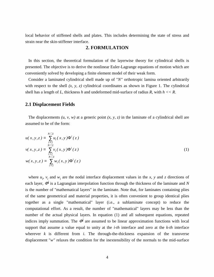
Consider a laminated cylindrical shell made up of "N" orthotropic lamina oriented arbitrarily

with respect to the shell (x, y, z) cylindrical coordinates as shown in Figure 1. The cylindrical

shell has a length of L, thickness h and undeformed mid-surface of radius R, with h << R.

2.1 Displacement Fields

The displacements (u, v, w) at a generic point (x, y, z) in the laminate of a cylindrical shell are

assumed to be of the form:

u( x , y , z ) u ( x , y ) ( z )ii 1

N 1i=

=

+

∑ Φ

v( x , y , z ) v ( x , y ) ( z )ii 1

N 1i=

=

+

∑ Φ (1)

w( x , y , z ) w ( x , y ) ( z )ii 1

N 1i=

=

+

∑ Φ

where ui, vi and wi are the nodal interface displacement values in the x, y and z directions of

each layer, Φi is a Lagrangian interpolation function through the thickness of the laminate and N

is the number of "mathematical layers" in the laminate. Note that, for laminates containing plies

of the same geometrical and material properties, it is often convenient to group identical plies

together as a single "mathematical" layer (i.e., a sublaminate concept) to reduce the

computational effort. As a result, the number of "mathematical" layers may be less than the

number of the actual physical layers. In equation (1) and all subsequent equations, repeated

indices imply summation. The Φi are assumed to be linear approximation functions with local

support that assume a value equal to unity at the i-th interface and zero at the k-th interface

wherever k is different from i. The through-the-thickness expansion of the transverse

displacement "w" relaxes the condition for the inextensibility of the normals to the mid-surface

5

as stipulated by the classical lamination theory and the shear deformation theories. This allows a

non-zero transverse normal strain as in the three-dimensional models. The transverse normal

stresses assume a very significant value (when compared to the allowable stress) in laminates

with localized effects, like cut-outs, free edges and skin-stiffener interfaces and need to be

considered.

The global linear approximation functions are defined as below:

Φ i

i i

ii i

i i

ii i

z

zz z

hz z z

zz z

hz z z

( )

( ) ,

( ) ,

( )

( )

==

−≤ ≤

=−

≤ ≤

− −

−−

+

ψ

ψ

21 1

11

1 1

( i = 1, 2, ... N) (2)

where ψ ji (j = 1, 2) is the local or layer Lagrange interpolation function associated with the j-th

node of the i-th layer and hi is the thickness of the i-th layer as shown in Figure 1.b. Here, it

could be recognized that each layer is in effect a one-dimensional finite element through thethickness. The ψ j

i are the interpolation functions of the i-th element where j = 1, 2 for linear

elements and j = 1, 2, 3 for quadrilateral elements.

2.2 Strain-Displacement Relationships

The von Kármán type of nonlinear strains are considered, where small strains and moderate

rotations with respect to the shell reference surface are assumed. Rotations about the normals to

the shell reference surface are considered to be negligible for cylinders where the ratio h/R is

considerably less than unity. Here h is the thickness and R is the radius of the cylindrical shell.

Note that any of the strain-displacement relationships documented in the literature could be used

depending on the h/R ratio. In this study, the Donnell type relationships are adopted. The Donnell

type strain-displacement equations in an orthogonal cylindrical coordinate system are:

ε ∂∂

∂∂

∂∂

∂∂

∂∂xx

i i i j i ju

x

w

x

u

x

w

x

w

x= + = +1

2

1

22( ) Φ Φ Φ

ε ∂∂

∂∂

∂∂

∂∂

∂∂yy

i i i i j i jv

y

w

R

w

y

v

y

w

R

w

y

w

y= + + = + +1

2

1

22( ) ( )Φ Φ Φ

γ ∂∂

∂∂

∂∂

∂∂

∂∂

∂∂

∂∂

∂∂xy

i i i i j i ju

y

v

x

w

x

w

y

u

y

v

x

w

y

w

x= + + = + +( )Φ Φ Φ (3)

6

γ ∂∂

∂∂

∂∂yz i

ii i iv

z

w

y

v

Rv

d

dz

w

y

v

R= + − = + −Φ Φ( )

7

Z

1

2

N+1

layer 1

layer N

Y

3

a) Notations for a cylindrical shell

Figure 1. Geometry, coordinate system and notations for a stiffened cylindrical shell.

X R

Z

Y

L

layer 1

layer 2

layer 3

layer 4

interface 1

2

3

4

5

Φ 1

Φ 2

Φ 3

Φ 4

Φ 5

ψ 1

2

ψ 1

1

Z h

1

b) 1-D approximation functions

c) Geometry of cylindrical shell

8

γ ∂∂

∂∂

∂∂xz i

ii iu

z

w

xu

d

dz

w

x= + = +Φ Φ and

ε ∂∂zz i

iw

zw

d

dz= = Φ

2.3 Constitutive Equations

The three-dimensional constitutive equations of an arbitrarily oriented orthotropic laminae in

the laminate coordinate system are:

σσσσ

εεεγ

xx

yy

zz

xy

xx

yy

zz

xy

C C C C

C C C C

C C C C

C C C C

=

11 12 13 16

12 22 23 26

13 23 33 36

16 26 36 66

(4.a)

σσ

γγ

yz

xz

yz

xz

C C

C C

=

44 45

45 55

(4.b)

Note that transformed reduced stiffnesses C16, C26, C36 and C45 are all equal to zero for laminae

whose material coordinate axes coincide with the coordinate axis of the shell.

2.4 Virtual Work Statement

The virtual work statement can be written using Hamilton’s principle. The stationary total

potential energy principle dictates that δΠ = 0, where δΠ is the first variation of the total

potential energy,

δΠ = δU + δV (5)

The virtual strain energy of the shell due to the internal in-plane, transverse shear and

transverse normal stresses is δU and is given as:

δ σ δε σ δε σ δε σ δγ σ δγ σ δγU dzdAxx xx yyh

h

yy zz zz xz xz yz yz xy xy= + + + + +−

∫∫ ( )

2

2

Ω

(6)

9

Here Ω is the reference surface of the shell. The work done by the specified pre-bucklingstresses σi is of the form:

δ σ δεV dz dAih

h

i=−

∫∫ ( )

2

2

Ω

(7)

Substituting the strain-displacement relations (3) into the total potential energy given by

equations (5), (6) and (7) gives the following weak form of the virtual work statement which will

later be used to derive the equations of motion and the finite element model:

0 = + + + + + +

+ + + + + +

+ − +

∫ [ ( ) ( )

( )

( )

Nu

xN

v

y

w

RN

u

y

v

RM

w

x

w

xM

w

y

w

y

Mw

x

w

y

w

y

w

xQ u Q w Q v K

w

x

Kw

y

v

RM

w

xi i

yi i i

xyi i i

xij i j

yij i j

xyij i j i j

xzi

i zzi

i yzi

i xzi i

yzi i i

xij

∂δ∂

∂δ∂

∂ ∂δ∂

δ ∂δ∂

∂∂

∂δ∂

∂∂

∂δ∂

∂∂

∂δ∂

∂∂

δ δ δ∂δ∂

∂δ∂

δ ∂δ

Ω

]i j

yij i j

xyij i j i j

i ix

w

xM

w

y

w

yM

w

x

w

y

w

y

w

xP w dA

∂∂∂

∂δ∂

∂∂

∂δ∂

∂∂

∂δ∂

∂∂

δ+ + + +( )

(8)

where Pi is the pressure applied on the shell surface. For internal pressure, i =1 and for external

pressure, i = N+1. The laminate force and moment resultants are the results of integration of the

stresses through the thickness of the laminate and are given in terms of the internal stresses and

the interpolation polynomials as:

( , , ) ( , , )N N N dzxi

yi

xyi

xxh

h

yy xyi=

−

∫ σ σ σ

2

2

Φ ,

( , , ) ( , , )M M M dzxij

yij

xyij

xxh

h

yy xyi j=

−

∫ σ σ σ

2

2

Φ Φ

( , , ) ( , , )Q Q Qd

dzdzxz

iyzi

zzi

xzh

h

yz zz

i

=−

∫ σ σ σ

2

2 Φ, ( , ) ( , )K K dzxz

iyzi

xzh

h

yzi=

−

∫ σ σ

2

2

Φ (9)

10

( , , ) ( , , )M M M dzxij

yij

xyij

xxh

h

yy xyi j=

−

∫ σ σ σ

2

2

Φ Φ

The laminate forces given in equation (9) could be expressed in terms of displacements instead

of stresses. This will prove convenient later on when the finite element model is formulated in

section 2.10. Substituting the constitutive relations given by equation (4) into the force resultants

of equation (9) gives an expression for the laminate force resultants in terms of the

displacements:

N Au

xA

v

y

w

RA w A

u

y

v

x

Dw

x

w

xD

w

y

w

yD

w

x

w

y

xi ij j ij j j ij

jij j j

ijk j k ijk j k ijk j k

= + + + + +

+ + +

11 12 13 16

11 12 16

1

2

1

2

∂∂

∂∂

∂∂

∂∂

∂∂

∂∂

∂∂

∂∂

∂∂

∂∂

( ) ( )

N Au

xA

v

y

w

RA w A

u

y

v

x

Dw

x

w

xD

w

y

w

yD

w

x

w

y

yi ij j ij j j ij

jij j j

ijk j k ijk j k ijk j k

= + + + + +

+ + +

12 22 23 26

12 22 26

1

2

1

2

∂∂

∂∂

∂∂

∂∂

∂∂

∂∂

∂∂

∂∂

∂∂

∂∂

( ) ( )

Q Au

xA

v

y

w

RA w A

u

y

u

x

Dw

x

w

xD

w

y

w

yD

w

x

w

y

zzi ji j ji j j ji

jji j j

jki j k jki j k jki j k

= + + + + +

+ + +

13 23 33 36

13 23 36

1

2

1

2

∂∂

∂∂

∂∂

∂∂

∂∂

∂∂

∂∂

∂∂

∂∂

∂∂

( ) ( )

Q A u Aw

xA v A

w

y

v

Rxzi ij

jji j ij

jji j j= + + + −55 55 45 45

∂∂

∂∂

( )

Q A u Aw

xA v A

w

y

v

Ryzi ij

jji j ij

jji j j= + + + −45 45 44 44

∂∂

∂∂

( ) (10)

K A u Aw

xA v A

w

y

v

Rxzi ij

jji j ij

jji j j= + + + −55 55 45 45

∂∂

∂∂

( )

K A u Aw

xA v A

w

y

v

Ryzi ij

jji j ij

jji j j= + + + −45 45 44 44

∂∂

∂∂

( )

M Du

xD

v

y

w

RD w D

u

y

v

x

Fw

x

w

xF

w

y

w

yF

w

x

w

y

xij ijk k ijk k k ijk

kijk k k

ijkl k l ijkl k l ijkl k l

= + + + + +

+ + +

11 12 13 16

11 12 16

1

2

1

2

∂∂

∂∂

∂∂

∂∂

∂∂

∂∂

∂∂

∂∂

∂∂

∂∂

( ) ( )

11

M Du

xD

v

y

w

RD w D

u

y

v

x

Fw

x

w

xF

w

y

w

yF

w

x

w

y

yij ijk k ijk k k ijk

kijk k k

ijkl k l ijkl k l ijkl k l

= + + + + +

+ + +

12 22 23 26

12 22 26

1

2

1

2

∂∂

∂∂

∂∂

∂∂

∂∂

∂∂

∂∂

∂∂

∂∂

∂∂

( ) ( )

M Du

xD

v

y

w

RD w D

u

y

v

x

Fw

x

w

xF

w

y

w

yF

w

x

w

y

xyij ijk k ijk k k ijk

kijk k k

ijkl k l ijkl k l ijkl k l

= + + + + +

+ + +

16 26 36 66

16 26 66

1

2

1

2

∂∂

∂∂

∂∂

∂∂

∂∂

∂∂

∂∂

∂∂

∂∂

∂∂

( ) ( )

The laminate stiffness coefficients used in equations (10) are given in terms of the elastic

constants and the Lagrange interpolation functions and their derivatives as:

A C dzmnij

mnh

h

i j=−

∫2

2

Φ Φ , A Cd

dzdzmn

ijmn

h

h

ij

=−

∫2

2

ΦΦ

,

A Cd

dz

d

dzdzmn

ijmn

h

h

i j

=−

∫2

2 Φ Φ, D C dzmn

ijkmn

h

h

i j k=−

∫2

2

Φ Φ Φ , (11)

D Cd

dzdzmn

ijkmn

h

h

i jk

=−

∫2

2

Φ ΦΦ

and F C dzmnijkl

mnh

h

i j k l=−

∫2

2

Φ Φ Φ Φ

Here i, j, k, l = 1, 2, ..., N+1 and m, n = 1, 2, ..., 6. Note that the laminate stiffness matrices with

single bars on them are not symmetric with respect to the superscripts, whereas all the other

matrices are symmetric with respect to both the superscripts and subscripts. The symmetry in the

subscripts is, of course, due to the symmetry in the elastic constants of the material of the

laminates. The definition of the integrals in equation (11) accounts for the symmetry in the

superscripts for all the laminate stiffness coefficients except the ones with single bars on them.

2.5 Equations of Motion

The Euler-Lagrange equations of motion of the layerwise shell theory are obtained by

integrating by parts the derivatives of the various quantities of the weak form given by equation

12

(8) and collecting the coefficients of δu, δv, and δw separately. The equations of motion, thus

obtained, are:

0 = + −∂∂

∂∂

N

x

N

yQx

iyi

xzi (12a)

01= + − +

∂∂

∂∂

N

x

N

yQ

RKxy

iyi

yzi

yzi (12b)

qK

x

K

y RN Q

xM

w

xM

w

y yM

w

yM

w

xixzi

yzi

yi

zzi

xij j

xij j

yij j

xyij j= + − + + + + +∂

∂∂

∂∂∂

∂∂

∂∂

∂∂

∂∂

∂∂

( ) ( ) ( )1

(12c)

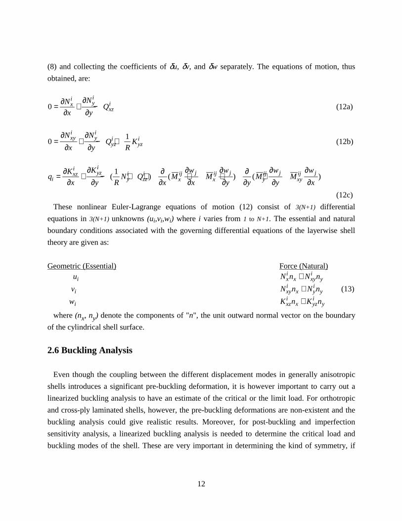
These nonlinear Euler-Lagrange equations of motion (12) consist of 3(N+1) differential

equations in 3(N+1) unknowns (ui,vi,wi) where i varies from 1 to N+1. The essential and natural

boundary conditions associated with the governing differential equations of the layerwise shell

theory are given as:

Geometric (Essential) Force (Natural) ui N n N nx

ix xy

iy+

vi N n N nxyi

x yi

y+ (13)

wi K n K nxzi

x yzi

y+

where (nx, ny) denote the components of "n", the unit outward normal vector on the boundary

of the cylindrical shell surface.

2.6 Buckling Analysis

Even though the coupling between the different displacement modes in generally anisotropic

shells introduces a significant pre-buckling deformation, it is however important to carry out a

linearized buckling analysis to have an estimate of the critical or the limit load. For orthotropic

and cross-ply laminated shells, however, the pre-buckling deformations are non-existent and the

buckling analysis could give realistic results. Moreover, for post-buckling and imperfection

sensitivity analysis, a linearized buckling analysis is needed to determine the critical load and

buckling modes of the shell. These are very important in determining the kind of symmetry, if

13

any, to be used for analysis. Symmetry should be exploited as much as possible in full nonlinear

analysis to reduce the computational expenses and effort.

Reddy [17] has shown that the pre-buckling stress state specified below corresponds to a pure

membrane state for which the end effects could be ignored:

σxx = - qo ; σyy = (P1 + P

N+1) R/h and σxz = σyz = σxy = σzz = 0 (14)

The work done by these pre-buckling stresses can be written as:

δ∂∂

∂δ∂

∂∂

∂δ∂

W Mw

x

w

xM

w

y

w

ydxdyx

ij i j

yij i j= +∫ ( )

Ω

(15)

where the moment resultants M xij and M y

ij are themselves functions of the buckling loads and the

through-the-thickness interpolation functions Φ i and are given as:

M q dZxij

oi j

h

h

= −−∫ Φ Φ

2

2

and M P PR

hdZy

ijN

i j

h

h

= − ++−∫( )1 1

2

2

Φ Φ (16)

Note that the indices i and j vary from 1 to N+1, where N is the number of mathematical layers

in the shell. The virtual work due to pre-buckling stresses will be used to derive the geometry

stiffness matrix in a finite element formulation.

2.7 Natural Vibration Analysis

It is often desired to determine the fundamental vibration mode and frequency of a cylindrical

shell through an eigenvalue analysis. This could be done by deriving the virtual work statement

due to the total potential energy and kinetic energy. The principle of virtual displacements

dictates that the time integral of the total potential energy and the kinetic energy vanishes:

00

= −∫ ( )δ δU K dtT

(17)

The total potential energy, δU, is as defined in equation (6). The kinetic part, δK, is given by:

14

δ ρ δ δ δKdt u u v v w w dzdAdtT

i

h

hT

ii

jj

ii

jj

ii

jj= + +∫ ∫∫∫

−02

2

0 Ω

Φ Φ Φ Φ Φ Φ( )( & ) ( )( & ) ( )( & ) (18)

where ρ i is the density of the composite material of the i-th lamina.

2.8 Finite Element Model

The interface displacements (ui, vi, wi) are expanded over each element as a linear combination

of the surface-wise two-dimensional Lagrange interpolation functions ϕj and the nodal interface

displacements (uij, vi

j, wij) as follows:

( , , ) ( , , )u v w u v wi i i ij

ij

ij

j

p

j==∑

1

ϕ (19)

where p is the number of nodes in each element. The variational form of the virtual work

statement, i.e., equation (8), is developed by multiplying it with a test function and integrating the

results by parts. The finite element model is then developed by substituting Equations (19) and

(12) (i.e., the equations of motion and the displacement expansions, respectively) into the

resulting variational form as:

11 12 13

21 22 23

31 32 33

K K K

K K K

K K K

u

v

w

q

q

q

ij ij ij

ij ij ij

ij ij ij

u

v

w

αβ αβ αβ

αβ αβ αβ

αβ αβ αβ

=

(20)

where i, j = 1, 2, ..., p and α, β = 1, 2, ..., N+1. The interface displacements vectors are given by

u, v and w, whereas the corresponding load vectors that consist of boundary and force

contributions are qu, qv and qw.

For eigenvalue analysis, the finite element model takes the form:

11 12 13

21 22 23

31 32 33

11

22

33

0 0

0 0

0 0

0

0

0

K K K

K K K

K K K

S

S

S

u

v

w

ij ij ij

ij ij ij

ij ij ij

ij

ij

ij

αβ αβ αβ

αβ αβ αβ

αβ αβ αβ

αβ

αβ

αβ

λ

−

=

(21)

15

For linearized buckling analysis, elements of the geometry matrix are defined as:

11 22 0S Sij ijαβ αβ= = and

33S Gx x

Gy y

dxdyiji j i jαβ αβ αβ∂ϕ

∂∂ϕ∂

∂ϕ∂

∂ϕ∂

= +∫ ( )Ω

(22)

For natural vibration analysis, the lowest λ is the square of the fundamental frequency and [S]

is the mass matrix, given in terms of the layer density and laminate mass coefficient as:

11 22 33S S S G dxdyij ij ij i jαβ αβ αβ α αβρ ϕ ϕ= = = ∫

Ω

( ) (23)

where ρα is the density of the composite material of layer-α. The laminate mass coefficients

Gαβ are functions of the through-the-thickness integration polynomials and are defined as:

G dzh

h

αβ α β=−

∫ Φ Φ

2

2

(24)

Note that the solution of the eigenvalue problem defined by equation (21) gives the eigenvalues

λαi . The minimum eigenvalue is the critical buckling load, Pcr, in the case of buckling analysis,

and the square of the fundamental frequency (i.e. ω2) in the case of natural vibration analysis.

The elements of the tangent stiffness matrix for a cylindrical shell element are given in

References [18] and [19].

2.9 Modeling of Stiffened Plates and Shells

Since both the shell and stiffener elements have the same displacement fields, compatibility of

strains and equilibrium of forces can be enforced by letting the two elements share the same

nodes in the finite element mesh. The one-dimensional layerwise stiffener elements share one of

the sides of the two-dimensional quadrilateral surface-wise shell elements. Depending on their

location (i.e., whether they are internal or external), the stiffener elements will again share one or

more of the through-thickness nodes of the skin element. Stiffeners attached to either the outside

or inside of the skin share one node whereas stiffeners attached to both sides of the skin share

two nodes through the thickness. Apart from enforcing compatibility of strains and equilibrium

of forces, the sharing of nodes significantly reduces the size of the equations to be assembled and

16

solved. Unlike analytical models which "smear" or average out the properties of the stiffeners

over the surface irrespective of the location of the stiffeners, the layerwise format of the stiffener

and shell skin element takes care of eccentricity automatically. The effect of the location of the

stiffeners is also handled readily by the model developed. The application of the layerwise

stiffener element for the analysis of stiffened composite plates and shells is discussed in detail by

Kassegne and Reddy [18].

3. NUMERICAL EXAMPLES

In this section, a number of plates and laminated cylindrical shells stiffened by stringers or

rings or a combination of them are analyzed for buckling and stresses. The stiffeners may be

located on the inside or outside of the shell skin. The solved examples illustrate that there is a

marked difference between the behavior of internally and externally stiffened shells. The

comparison is given wherever appropriate. The stiffeners are modeled as discrete unless

otherwise specified.

3.1 Buckling of Stiffened Orthotropic Plate

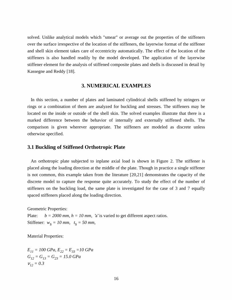
An orthotropic plate subjected to inplane axial load is shown in Figure 2. The stiffener is

placed along the loading direction at the middle of the plate. Though in practice a single stiffener

is not common, this example taken from the literature [20,21] demonstrates the capacity of the

discrete model to capture the response quite accurately. To study the effect of the number of

stiffeners on the buckling load, the same plate is investigated for the case of 3 and 7 equally

spaced stiffeners placed along the loading direction.

Geometric Properties:

Plate: b = 2000 mm, h = 10 mm, ’a’ is varied to get different aspect ratios.

Stiffener: ws = 10 mm, ts = 50 mm,

Material Properties:

E11 = 100 GPa, E22 = E33 =10 GPa

G12 = G13 = G23 = 15.0 GPa

ν12 = 0.3

17

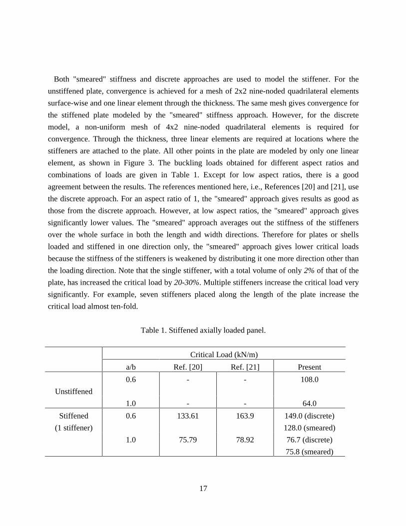
Both "smeared" stiffness and discrete approaches are used to model the stiffener. For the

unstiffened plate, convergence is achieved for a mesh of 2x2 nine-noded quadrilateral elements

surface-wise and one linear element through the thickness. The same mesh gives convergence for

the stiffened plate modeled by the "smeared" stiffness approach. However, for the discrete

model, a non-uniform mesh of 4x2 nine-noded quadrilateral elements is required for

convergence. Through the thickness, three linear elements are required at locations where the

stiffeners are attached to the plate. All other points in the plate are modeled by only one linear

element, as shown in Figure 3. The buckling loads obtained for different aspect ratios and

combinations of loads are given in Table 1. Except for low aspect ratios, there is a good

agreement between the results. The references mentioned here, i.e., References [20] and [21], use

the discrete approach. For an aspect ratio of 1, the "smeared" approach gives results as good as

those from the discrete approach. However, at low aspect ratios, the "smeared" approach gives

significantly lower values. The "smeared" approach averages out the stiffness of the stiffeners

over the whole surface in both the length and width directions. Therefore for plates or shells

loaded and stiffened in one direction only, the "smeared" approach gives lower critical loads

because the stiffness of the stiffeners is weakened by distributing it one more direction other than

the loading direction. Note that the single stiffener, with a total volume of only 2% of that of the

plate, has increased the critical load by 20-30%. Multiple stiffeners increase the critical load very

significantly. For example, seven stiffeners placed along the length of the plate increase the

critical load almost ten-fold.

Table 1. Stiffened axially loaded panel.

Critical Load (kN/m)

a/b Ref. [20] Ref. [21] Present

Unstiffened

0.6 - - 108.0

1.0 - - 64.0

Stiffened

(1 stiffener)

0.6 133.61 163.9 149.0 (discrete)

128.0 (smeared)

1.0 75.79 78.92 76.7 (discrete)

75.8 (smeared)

18

(3 stiffeners) 1.0 - - 471.0 (discrete)

(7 stiffeners) 1.0 - - 646.0 (discrete)

a

X, u

Y, v

b

Figure 2. Geometry and Loading of a Stiffened Orthotropic Plate.

v = w = 0

w = 0

u = w = 0

w = 0

w

h

Z, w

ts

19

Figure 3. Finite Element Mesh for a Stiffened Orthotropic Plate.

x

y

z

2@ 150 mm 2@350 mm

4 @500 mm

20

3.2 Symmetrically Stiffened Cantilever Shell

A cantilever shell stiffened by symmetrically located rings and stringers is analyzed by the

layerwise approach. The shell is loaded by a point load applied at one of the corners. This

produces an unsymmetrical complex displacement field which is a combination of membrane

stretching, bending and out-of-plane distortion. The capability of the model developed in this

study is well-tested by this particular bench-mark problem that has been solved by a number of

researchers [22-24]. Figure 4 gives the geometric details of the shell and the stiffeners. Note that

for this case where the rings and the stringers are placed symmetrically with respect to the mid-

plane of the shell skin, section A-A is identical to section B-B. The mesh adopted here consists

of four nine-noded quadrilateral layerwise shell elements. Through the thickness, two linear

elements per lamina are used. The results are summarized in Table 2 for the following data:

Material Properties: E = 1.0x106 Kg/cm2, ν = 0.3

t = 6.0 cm.

3.3 Eccentrically Stiffened Cantilever Shell

The same cantilever shell discussed in section 3.2 is stiffened by eccentric rings and symmetric

stringers. This introduces additional unsymmetrical deformations which are captured by the

layerwise model developed here quite accurately as shown in Table 3. The geometry of the ring is

shown in Figure 5. Note that sections A-A and B-B are different for this particular type of

stiffening scheme. The total thickness of the stringers, t , is 13 cm. for this case.

Table 3 summarizes the results obtained from the literature and the present study. Note that

there is a good agreement between the results of Ref. [23] and the current study. The

displacements reported in Ref. [22] are low because the stiffener elements which are obtained as

a degenerate case of a shell of revolution are torsionally stiff [24].

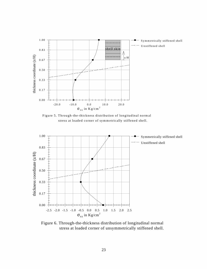
Figure 5 shows the through-thickness distribution of the normal stress σxx for the symmetrical

stiffening scheme and the unstiffened shell. The stresses are calculated at the loaded corner. It

can be seen that the stiffeners reduce the stresses drastically. The presence of the symmetric

stiffeners also alters the position of the neutral axis significantly. Most of the shell skin at the

loaded corner is now under compression. Figure 6 shows the distribution of σxx when eccentric

21

rings and symmetrical stringers are used. Note that, apart from reducing the magnitude of the

stresses drastically, this particular stiffening scheme alters the distribution of the stresses

qualitatively too. The position of the neutral axis is also shifted. Most of the shell skin at the

loaded corner is still under compression. The peak stress for this stiffening scheme is about

1/10-th of that corresponding to the symmetrically stiffened shell.

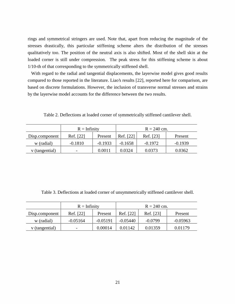
With regard to the radial and tangential displacements, the layerwise model gives good results

compared to those reported in the literature. Liao’s results [22], reported here for comparison, are

based on discrete formulations. However, the inclusion of transverse normal stresses and strains

by the layerwise model accounts for the difference between the two results.

Table 2. Deflections at loaded corner of symmetrically stiffened cantilever shell.

R = Infinity R = 240 cm.

Disp.component Ref. [22] Present Ref. [22] Ref. [23] Present

w (radial) -0.1810 -0.1933 -0.1658 -0.1972 -0.1939

v (tangential) - 0.0011 0.0324 0.0373 0.0362

Table 3. Deflections at loaded corner of unsymmetrically stiffened cantilever shell.

R = Infinity R = 240 cm.

Disp.component Ref. [22] Present Ref. [22] Ref. [23] Present

w (radial) -0.05164 -0.05191 -0.05440 -0.0799 -0.05963

v (tangential) - 0.00014 0.01142 0.01359 0.01179

22

10 Kg

X

Y

Z

A

A

B

B

a) Section A-A b) Section B-B

Figure 4. A Stiffened Cantilever Cylindrical Shell.

120 cm

6 cm

1 cm

1 cm

t

(for unsymmetrical case only)

23

F ig ure 5 . T h rou gh -th e-th ickn ess d istribu tion o f lon g itud in a l n orm al

-20 .0 -10 .0 0 .0 10 .0 2 0 .0

thic

knes

s co

ordi

nate

(z/

H)

0 .00

0 .17

0 .33

0 .50

0 .67

0 .83

1 .00 S y m m etrically stiffened shell

U n stiffened shell

σ xx in K g/cm 2

stress a t load ed co rner o f sy m m etrica lly stiffen ed she ll.

z /H

sh e ll sk in

Figure 6. Through-the-thickness distribution of longitudinal normal

-2.5 -2.0 -1.5 -1.0 -0.5 0.0 0.5 1.0 1.5 2.0 2.5

thic

knes

s co

ordi

nate

(z/

H)

0.00

0.17

0.33

0.50

0.67

0.83

1.00 Symmetrically stiffened shell

Unstiffened shell

σxx in Kg/cm2

stress at loaded corner of unsymmetrically stiffened shell.

24

3.4 Stiffened Cylindrical Panel Under a Point Load

A simply supported cylindrical roof panel is stiffened with stringers and rings and subjected to

a central point load of magnitude P = 150 Kips. A comparative study of the displacements at the

center of the panel is made for different locations of stringers and rings as summarized in Table

4. Figure 7 shows the geometry and the boundary conditions of the cylindrical panel. The

stiffeners have the same material property as that of the shell skin material.

A convergence study was performed by increasing the number of two-dimensional elements

surface-wise and one-dimensional elements through the thickness. Due to the steep gradient in

strains and stresses at and near the interface between the shell and the stiffeners, a non-uniform

mesh consisting of smaller elements near the stiffeners is used. The displacements converge for a

non-uniform mesh consisting of 16 nine-noded quadrilateral elements and 81 nodes as shown in

Figure 8. Through the thickness of the shell, two linear element per lamina are used.

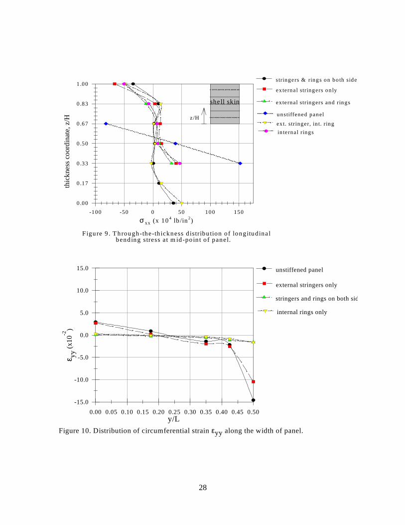
The distribution of the longitudinal normal stress σxx at the mid-point of the panel for different

stiffening schemes is given in Figure 9. The stiffeners have a significant effect on the distribution

of the stresses both qualitatively and quantitatively. All stiffening schemes reduce the

longitudinal normal stress quite significantly. With regard to reducing stresses, rings placed

externally and stringers placed internally provide the most efficient stiffening scheme. This

scheme reduces the peak stresses in the shell skin by as much as 1/100-th. Note also that further

drastic improvement could be obtained by using both internal and external stringers and rings.

Externally placed stringers are comparatively the least efficient.

With regard to the transverse displacement w, it can be observed that rings and stringers used

together internally and externally consecutively or vise versa result in the minimum

displacements and are therefore more efficient here. The least efficient stiffening scheme for this

particular case is where rings or stringers are used alone. With regard to the u and v

displacements, there is a clear indication that the neutral axis shifts significantly due to the

presence of the stiffeners. In most cases, the neutral axis even moves out of the shell skin plane,

resulting in the skin being totally in compression or tension.

In Figure 10, the distribution of the circumferential strain εyy along x = a/2 is plotted for

different stiffening schemes. The strain under consideration is evaluated at node number 5, i.e., at

the top of the shell skin (Figure 8). As expected, the strain peaks at the point of load application,

which is the mid-point of the cylindrical panel. The stiffeners tend to smooth out the peak. Rings,

however, play the major part in reducing the circumferential strain from a peak strain of 0.146 for

the unstiffened case down to 0.0181 for the case of a ring stiffened panel. In overall

25

considerations, a combination of stringers and rings placed alternately internally or externally

provides the most effective stiffening scheme.

Table 4. Effect of location of stiffeners on the displacement pattern of a cylindrical panel.

Unstiffened Stiffened

disp.(in

)

------- S1 S2 S3 S4 S5 S6

u1 - - - - -0.051 - -0.051

u2 - - - - -0.021 - -0.021

u3 -0.063 -0.049 -0.048 -0.041 -0.002 -0.041 -0.002

u4 0.001 -0.015 0.000 -0.010 0.010 -0.010 0.010

u5 0.064 0.007 0.046 0.001 0.040 0.002 0.040

u6 - 0.027 0.045 0.021 - 0.022 -

u7 - 0.061 0.044 0.051 - 0.052 -

v1 - - -0.067 -0.049 -0.049 - -0.049

v2 - - -0.030 -0.022 -0.022 - -0.022

v3 0.014 -0.022 0.010 0.007 0.008 -0.001 0.008

v4 0.026 -0.015 -0.029 -0.013 -0.014 -0.005 -0.014

v5 0.037 -0.008 -0.021 -0.021 -0.016 -0.044 -0.016

v6 - - - - - -0.024 -

v7 - - - - - 0.001 -

w1 - - -0.833 -0.617 -0.611 - -0.611

w2 - - -0.835 -0.618 -0.613 - -0.613

w3 -1.250 -0.789 -0.836 -0.618 -0.616 -0.658 -0.616

w4 -1.265 -0.798 -0.869 -0.627 -0.641 -0.657 -0.641

w5 -1.249 -0.790 --0.960 -0.625 -0.641 -0.629 -0.641

w6 - -0.792 - -0.626 - -0.625 -

w7 - -0.792 - -0.625 - -0.622 -

S1 - external stringers only, S2 - internal rings only

S3 - internal rings and external stringers, S4 - external rings and internal stringers

S5 - external rings and external stringers, S6 - internal rings and internal stringers.

26

Z

gure 7. Geometry of an orthotropic cylindrical panel stiffened by stringers and rings.

u = w = 0

P

v = w = 0

v = w = 0

X

Y

1 in.

1 in.

u = w = 0

1 in.

1 in.

Material Properties:

E11 = 40.0E+06 psi

E22 = E33 = 1.0E+06 psi

G12 = G13 = 0.6E+06 psi

R = 100 in.

G23 = 0.5E+05 psi

ν12 = ν13 = 0.25

ν23 = 0.25

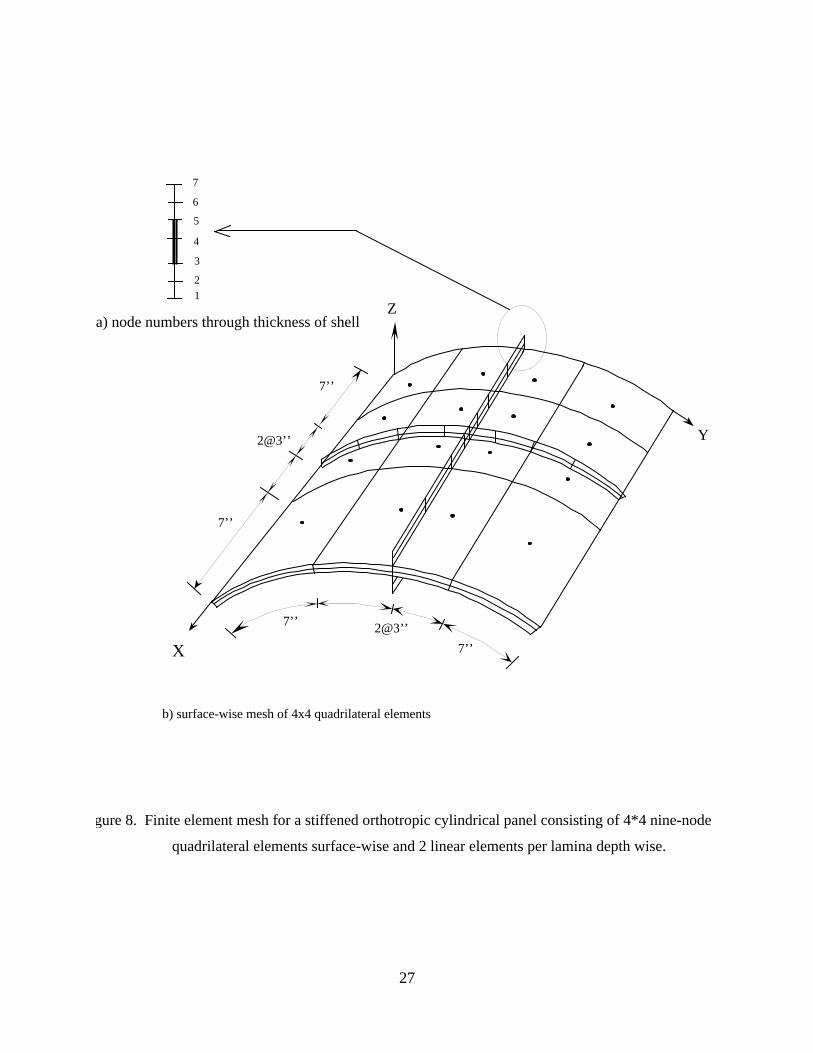
27

gure 8. Finite element mesh for a stiffened orthotropic cylindrical panel consisting of 4*4 nine-node

X

Y

Z

7’’

2@3’’

7’’

7’’

7’’

2@3’’

1

2

3

7

4

5

6

a) node numbers through thickness of shell

quadrilateral elements surface-wise and 2 linear elements per lamina depth wise.

b) surface-wise mesh of 4x4 quadrilateral elements

28

Figure 9 . T hrough-the-th ickness d istribution o f longitudina l

-100 -50 0 50 100 150

thic

knes

s co

ordi

nate

, z/H

0 .00

0 .17

0.33

0.50

0.67

0.83

1.00

ext. stringer, in t. ring

stringers & rings on bo th sides

ex terna l stringers on ly

external stringers and rings

unstiffened panel

in terna l rings

σ xx (x 10 4 lb /in 2)

bend ing stress a t m id -po in t o f panel.

z /H

she ll sk in

Figure 10. Distribution of circumferential strain εyy along the width of panel.

0.05 0.15 0.25 0.35 0.450.00 0.10 0.20 0.30 0.40 0.50

ε yy (x

10-2

)

-15.0

-10.0

-5.0

0.0

5.0

10.0

15.0

y/L

unstiffened panel

external stringers only

stringers and rings on both sid

internal rings only

29

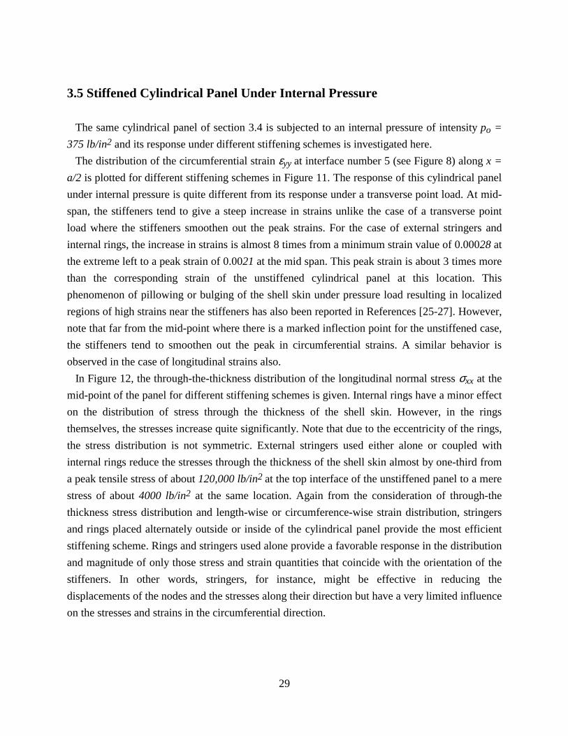
3.5 Stiffened Cylindrical Panel Under Internal Pressure

The same cylindrical panel of section 3.4 is subjected to an internal pressure of intensity po =

375 lb/in2 and its response under different stiffening schemes is investigated here.

The distribution of the circumferential strain εyy at interface number 5 (see Figure 8) along x =

a/2 is plotted for different stiffening schemes in Figure 11. The response of this cylindrical panel

under internal pressure is quite different from its response under a transverse point load. At mid-

span, the stiffeners tend to give a steep increase in strains unlike the case of a transverse point

load where the stiffeners smoothen out the peak strains. For the case of external stringers and

internal rings, the increase in strains is almost 8 times from a minimum strain value of 0.00028 at

the extreme left to a peak strain of 0.0021 at the mid span. This peak strain is about 3 times more

than the corresponding strain of the unstiffened cylindrical panel at this location. This

phenomenon of pillowing or bulging of the shell skin under pressure load resulting in localized

regions of high strains near the stiffeners has also been reported in References [25-27]. However,

note that far from the mid-point where there is a marked inflection point for the unstiffened case,

the stiffeners tend to smoothen out the peak in circumferential strains. A similar behavior is

observed in the case of longitudinal strains also.

In Figure 12, the through-the-thickness distribution of the longitudinal normal stress σxx at the

mid-point of the panel for different stiffening schemes is given. Internal rings have a minor effect

on the distribution of stress through the thickness of the shell skin. However, in the rings

themselves, the stresses increase quite significantly. Note that due to the eccentricity of the rings,

the stress distribution is not symmetric. External stringers used either alone or coupled with

internal rings reduce the stresses through the thickness of the shell skin almost by one-third from

a peak tensile stress of about 120,000 lb/in2 at the top interface of the unstiffened panel to a mere

stress of about 4000 lb/in2 at the same location. Again from the consideration of through-the

thickness stress distribution and length-wise or circumference-wise strain distribution, stringers

and rings placed alternately outside or inside of the cylindrical panel provide the most efficient

stiffening scheme. Rings and stringers used alone provide a favorable response in the distribution

and magnitude of only those stress and strain quantities that coincide with the orientation of the

stiffeners. In other words, stringers, for instance, might be effective in reducing the

displacements of the nodes and the stresses along their direction but have a very limited influence

on the stresses and strains in the circumferential direction.

30

F igu re 11 . D istribu tion o f c ircum feren tia l stra in fo r a

0 .0 0 .1 0 .2 0 .3 0 .4 0 .5

ε yy (x

10-2

)

-0 .50

-0 .25

0 .00

0 .25

0 .50

0 .75

1 .00

y /L

unstiffened panel

ex t. stringers and in

in ternal ring on ly

stiffened panel under in ternal p ressu re.

Figure 12. Through-the-thickness distribution of longitudinal

-15 -10 -5 0 5 10 15

thic

knes

s co

ordi

nate

, z/H

0.00

0.17

0.33

0.50

0.67

0.83

1.00 unstiffened panel

ext. stringer, int. ring

external stringers

σxx (x 104 lb/in2)

bending stress at mid-point of panel under internal pressure.

internal stringersz/H

shell skin

31

Figure 13. Distribution of σxx across the surface of a panel under internal pressure.

-45000.0-30000.0-15000.00.015000.030000.045000.060000.0

0.02.5

5.07.5

10.012.5

15.017.5

20.0

2.55.07.510.012.515.017.520.0

X AxisY-Axis

location of stringerslocation of ring

Figure 14. Distribution of σxx across the surface of a panel under a point load.

-3e+5-2e+5-2e+5-1e+5-5e+40e+05e+41e+5

0.02.5

5.07.5

10.012.5

15.017.5

20.0

0.0 2.5 5.0 7.5 10.0 12.5 15.0 17.5 20.0

X Axis

Y-Axis

location of ring

location of stringer

32

Figure 13 and 14 show the variation of the longitudinal bending stress σxx across the surface

of the cylindrical panel under internal pressure and a point load, respectively. The stiffening

scheme for the cylindrical panel consists of stringers and rings located both internally and

externally. The stresses shown in the figures are evaluated at the surface of the shell skin (i.e.,

interface number 5 in Figure 8).

As expected, the longitudinal bending stresses for both loading cases are zero at y = 0, L

where the in-plane displacement u has been specified as zero. There are two distinct regions

where the longitudinal bending stresses peak. The first region is at the (x = 0, L) boundary with

y = L/2 where the in-plane displacement u assumes its maximum value. The stiffener

intersection areas are the second region of high bending stresses for both loading types. For the

stiffening scheme adopted here, the stresses in these intersection areas are much higher than

anywhere in the shell skin.

3.5 Stiffened Cylindrical Panel Under Internal Pressure A nine layer composite cylindrical shell of lamination scheme (90/0/90/0/90/0/90/0/90)

stiffened by a single internal ring and a stringer (both of them of lamia of orientation of

0/90/0/90/0) and subjected to an internal pressure of 100 psi is solved here using the layerwise

approach. The same problem was originally solved by Goswami and Mukhopadhyay [23]. The

composite cylinder is simply supported on all sides.

The materal properties are given in Figure 15. A quarter model of a uniform mesh of 4x4 nine-

node quadrilateral elements is used surface-wise. The stiffners are modeled by a total of five

linear elements through the thickness. Only a single linear element is used through the thickness

of each lamina to arrive at a manageable size of system equations. The use of, for example, two

linear elements for each lamina of both the shell skin and the stiffneres increases the size of the

system equations to 7047x675, a rather large size which doesn’t fit in the memory of a

conventional PC, particularly if double precision arithmetics is used. The deflection profile

along the center line of the shell is given in Figure 16. Figure 17 shows the depth-wise

distribution of the circumferential stress σyy at the Gauss point near the top skin of the shell. At

this location, a significant amount of stresses are developed in the laminae of the rings whose

thickness is only 10% that of the shell skin. Note also that the major part of the remaining

lamina forces are taken by the plies in the vicinity of the interface between the stiffeners and the

shell skin. The stresses reduce quite significantly near the top of the shell skin.

33

Material Properties:

E11 = 40 Ksi

E22 = 1 Ksi

G12 = 0.6 Ksi

ν12 = 0.25

R = 100 in

h = 0.1 in

a = 10 in

Figure 15. Geometry of a Laminated Composite Cylindrical Shell.

Node (interface) 1

Node (interface) 15

b) linear Lagrange FEs (through the thickness)

a) stiffened shell (90/0/90/0/90/0/90/0/90)

v = w = 0

u = w = 0

u = w = 0

v = w = 0

X

Y

a

900

900900

90

0900

0

900

90

0.1 in.

1 in.

34

F ig u re 1 6 . D eflec tio n p ro file a lo n g th e cen te r lin e o f sh e ll.

0 .0 0 0 .0 5 0 .1 0 0 .1 5 0 .2 0 0 .2 5 0 .3 0 0 .3 5 0 .4 0 0 .4 5 0 .5 0

Cen

ter

Def

lect

ion

(x10

0)

-1 0 .0

-8 .0

-6 .0

-4 .0

-2 .0

0 .0

Y /L

L ay erw ise S h e ll T h e

R efe ren ce [2 3 ]

-300 0 .0 -225 0 .0 -1500 .0 -7 50 .0 0 .0 750 .0 1 500 .0

z-co

ordi

nate

(in

.)

0 .00 0

0 .12 5

0 .25 0

0 .37 5

0 .50 0

0 .62 5

0 .75 0

0 .87 5

1 .00 0

F igu re 17 . D ep th -w ise D istribu tion o f σ yy a t cen te r o f she ll.

σ yy (lb /in** 2 )

ins ide stiffen ers

in shell sk in

stresses

35

4. CONCLUSIONS

1. The Layerwise Theory of Reddy is capable of modeling the three-dimensional kinematics

and state of stress in cylindrical shells and stiffener elements to a high degree of accuracy. Unlike

the conventional equivalent single-layer methods, the layerwise theory, by virtue of its layerwise

format, gives detailed information on the state of stress and displacement field at each interface

in the shell skin and the stiffeners.

2. The behavior of stiffened panels and shells near the area of attachment of the shell skin and

the stiffeners is complex and only a discrete model is capable of capturing the response

accurately. In a very localized region near the stiffeners, there is a steep increase in strains for

shells under pressure. This is due to pillowing of the shell skin under the pressure load.

Quantification of these strains is very important in the design of stiffened composite shells due to

the brittle nature and low transverse strength exhibited by the fiber composite materials of which

they are made. Models based on an "average-stiffness" approach cannot accurately determine

local variations of stresses and strains, even though they tend to give satisfactory results for

global responses. The results reported in this research support the fact that a layerwise theory

using discrete stiffener formulation captures this local deep stress and starin gradient quite

accurately.

3. The eccentricity and location of both axial and circumferential stiffeners have a very

significant bearing on the response of stiffened shells. For transverse loading, external axial

stiffeners and internal rings or internal stringers and external rings used together are more

efficient, whereas under hydrostatic loads, internal rings used alone or together with external

stringers respond better. Stringers are very effective in reducing the longitudinal strains but have

almost negligible effect on the circumferential strains. On the other hand, rings have little effect

on the distribution of the longitudinal strains but they do reduce circumferential strains

significantly. A layerwise format handles the eccentricity and the location of the stiffeners

readily.

4. Unlike the equivalent single-layer methods, which can determine the stresses and strains

explicitly only at the top and bottom of the shell skin, the layerwise theory for discretely stiffened

cylindrical shells has the ability to accurately determine the variation of the stresses and strains

through the thickness of the stiffeners and the shell skin. Information on the state of stress and

strain through the thickness of the stiffeners and the shell skin is very important for the designer

who has to decide on the particular lamination scheme to be used for the stiffeners and the shell.

36

5. For shells with a large number of stiffeners, the discrete model might be expensive

computationally, especially at the design stage where cycles of analyses might have to be

performed. Therefore, a "smeared" model might be used as an economical alternative for analysis

at the preliminary design stage. The use of possible symmetry lines and axes might alleviate this

problem to some extent. For the final analysis, the discrete model may be used to obtain an

accurate and complete picture of the response of the stiffened plate or shell under the external

destabilizing loads.

6. In the example problems visited in this study, a perfect bond between the shell skin and the

stiffeners is assumed. For cases where adhesives which result in secondary bonding are used, the

adhesive layer should be modeled as a separate layer with its own material properties.

5. REFERENCES

1. A. E. H. Love, On the Small Free Vibrations and Deformations of Elastic Shells.Philosophical Transaction of the Royal Society (London), Series A, 17, 491-549 (1888).

2. J. N. Reddy and C. F. Liu, A Higher-order Theory for Geometrically Nonlinear Analysis ofComposite Laminates. NASA Contractor Report 4056, (1987).

3. A. Van der Neut, The General Instability of Stiffened Cylindrical Shells under AxialCompression. National Aeronautical Research Institute (Amsterdam), Report Series 314(1947).

4. P. C. Kohnke and W. C. Schnobrich, Analysis of Eccentrically Stiffened Cylindrical Shells.Journal of the Structural Division, ASCE, 98, 1493-1510 (1972).

5. K. P. Rao, A Rectangular Laminated Anisotropic Shallow Thin Shell Finite Element.Computer Methods in Applied Mechanics and Engineering, 15, 13-33 (1978).

6. A. Venkatesh and K. P. Rao, A Laminated Anisotropic Curved Beam and Shell StiffeningFinite Element. Computers and Structures, 15, 197-201 (1982).

7. A. Venkatesh and K. P. Rao, Analysis of Laminated Shells with Laminated Stiffeners UsingRectangular Finite Elements. Computers Methods in Applied Mechanics and Engineering,38, 255-272 (1983).

8. A. Venkatesh and K. P. Rao, A Doubly Curved Quadrilateral Finite Element for the Analysisof Laminated Anisotropic Thin Shells of Revolution. Computers and Structures, 12, 825-832(1980).

9. A. J. Carr and R. W. Clough, Dynamic Earthquake Behavior of Shell Roofs. Fourth WorldConference on Earthquake Engineering, Santiago, Chile (1969).

10. L. A. Schmit, Developments in Discrete Element Finite Deflection Structural Analysis byFunctional Minimization. Technical Report AFFDL-TR-68-126, Wright-Patterson Air ForceBase, Ohio (1968).

37

11. G. H. Ferguson and R. H. Clark, A Variable Thickness Curved Beam and Shell StiffeningElement with Shear Deformations. International Journal for Numerical Methods inEngineering, 14, 581-592 (1979).

12. S. Ahmad, B. M. Irons and O. C. Zienkiewicz, Analysis of Thick and Thin Shell Structuresby Curved Finite Elements. International Journal for Numerical Methods in Engineering, 2,419-451 (1970).

13. C. L. Liao, An Incremental Total Lagrangian Formulation for General Anisotropic Shell-Type Structures. AIAA Journal, 2, 435-453 (1989).

14. J. N. Reddy, A Generalization of Two-Dimensional Theories of Laminated CompositeLaminates. Communications in Applied Numerical Methods, 3, 173-180 (1987).

15. D. H. Robbins and J. N. Reddy, Modeling of Thick Composite Using a Layerwise LaminateTheory. International Journal for Numerical Methods in Engineering, 36, 655-677 (1993).

16. S. K. Kassegne and J. N. Reddy, A Layerwise Shell Stiffener and Stand-Alone Curved BeamElement. Computers and Structures, submitted for publication (December, 1995).

17. J. N. Reddy, A Layerwise Shell Theory with Applications to Buckling and Vibration ofCross-Ply Laminated Stiffened Circular Cylindrical Shells. CCMS-92-01, VirginiaPolytechnic Institute and State University (1992).

18. S. K. Kassegne and J. N. Reddy, Layerwise Theory for Discretely Stiffened LaminatedCylindrical Shells. CCMS-93-02, Virginia Polytechnic Institute and State University (1993).

19. S. K. Kassegne, Layerwise Theory for Discretely Stiffened Laminated Cylindrical Shells.Ph.D. Thesis, Virginia Polytechnic Institute and State University, Blacksburg, VA (1992).

20. B. Tripathy and K. P. Rao, Stiffened Composite Cylindrical Panels-Optimum Lay-up forBuckling by Ranking. Computers and Structures, 42, 481-488 (1978).

21. S. G. Lekhnitskii, S. W. Tsai and T. Cheron. Anisotropic Plates, Second Edition, Chapter 16,492-502 (1968).

22. C-L. Liao, Incremental Total Lagrangian Formulation for General Anisotropic Shell-TypeStructures. Ph.D. Thesis, Virginia Polytechnic Institute and State University, Blacksburg, VA(1987).

23. S. Goswami and M. Mukhopadhyay, Finite Element Analysis of Laminated CompositeStiffened Shell. Journal of Reinforced Plastics and Composites, 13, 574-616 (1994).

24. A. Bhimaraddi, A. J. Carr and P. J. Moss, Finite Element Analysis of Laminated Shells ofRevolution with Laminated Stiffeners. Computers and Structures, 33, 295-305 (1989).

25. J. T-S. Wang and T. M. Hsu, Discrete Analysis of Stiffened Composite Cylindrical Shells.AIAA Journal, 23, 1753-1761 (1985).

26. R. P. Ley, Analysis and Optimal Design of Pressurized, Imperfect, Anisotropic Ring-Stiffened Cylinders. Ph.D. Thesis, Virginia Polytechnic Institute and State University,Blacksburg, VA (1987).

27. M. W. Hyer, D. C. Loup and J. H. Starnes, Jr., Stiffener/Skin Interactions in Pressure LoadedComposite Panels. AIAA Journal, 28, 532-537 (1990).