load sensitivity studies and contingency analysis in · pdf fileload sensitivity studies and...
TRANSCRIPT
Load Sensitivity Studies and Contingency Analysis in Power Systems
by
Parag Mitra
A Dissertation Presented in Partial Fulfillment
of the Requirements for the Degree
Doctor of Philosophy
Approved August 2016 by the
Graduate Supervisory Committee:
Vijay Vittal, Chair
Gerald Heydt
Raja Ayyanar
Jiangchao Qin
ARIZONA STATE UNIVERSITY
December 2016

i
ABSTRACT
The past decades have seen a significant shift in the expectations and requirements
related to power system analysis tools. Investigations into major power grid disturbances
have suggested the need for more comprehensive assessment methods. Accordingly, sig-
nificant research in recent years has focused on the development of better power system
models and efficient techniques for analyzing power system operability. The work done in
this report focusses on two such topics
1. Analysis of load model parameter uncertainty and sensitivity based param-
eter estimation for power system studies
2. A systematic approach to n-1-1 analysis for power system security assess-
ment
To assess the effect of load model parameter uncertainty, a trajectory sensitivity
based approach is proposed in this work. Trajectory sensitivity analysis provides a system-
atic approach to study the impact of parameter uncertainty on power system response to
disturbances. Furthermore, the non-smooth nature of the composite load model presents
some additional challenges to sensitivity analysis in a realistic power system. Accordingly,
the impact of the non-smooth nature of load models on the sensitivity analysis is addressed
in this work. The study was performed using the Western Electricity Coordinating Council
(WECC) system model. To address the issue of load model parameter estimation, a sensi-
tivity based load model parameter estimation technique is presented in this work. A de-
tailed discussion on utilizing sensitivities to improve the accuracy and efficiency of the
parameter estimation process is also presented in this work.

ii
Cascading outages can have a catastrophic impact on power systems. As such, the
NERC transmission planning (TPL) standards requires utilities to plan for n-1-1 outages.
However, such analyses can be computationally burdensome for any realistic power system
owing to the staggering number of possible n-1-1 contingencies. To address this problem,
the report proposes a systematic approach to analyze n-1-1 contingencies in a computa-
tionally tractable manner for power system security assessment. The proposed approach
addresses both static and dynamic security assessment. The proposed methods have been
tested on the WECC system.

iii
DEDICATION
Dedicated to my mom Krishna Mitra and my dad Late Ratan Lal Mitra. Without
their encouragement and selflessness none of this could have been achieved.

iv
ACKNOWLEDGMENTS
I would like to offer my deepest gratitude to Dr. Vijay Vittal for providing me with
the opportunity to work on this project. It has truly been an enriching experience for me.
Dr. Vittal has been a continuous source of encouragement and guidance. Without his ef-
forts and insightful feedback, this work would not have been possible.
I would like to thank Dr. Gerald Heydt, Dr. Raja Ayyanar and Dr. Jiangchao Qin,
for taking out time to review this work and for being on my graduate supervisory commit-
tee.
I would also like to thank Dr. Daniel Tylavsky and Dr. Jennie Si, for taking out
time to review this work and for being on my comprehensive examination committee.
I would like to thank Pouyan Pourbiek and Anish Gaikwad from EPRI for provid-
ing constant guidance and valuable comments during my research. I would also like to
thank Brian Keel and Jeni Mistry from SRP for providing important data and evaluating
this research work at different stages. Special thanks to Dr. John Undrill for his invaluable
insights, ideas and encouragement.
I would like to thank EPRI and SRP for providing financial assistance during the
course of this work.
I am deeply indebted to my parents Late Mr. Ratan Lal Mitra and Dr (Mrs.) Krishna
Mitra for their love and support. I am also indebted to my elder brother Anurag Mitra and
sister-in-law Priyanka Mitra for their constant encouragement and help. Last but not the
least; I am thankful to all my friends for supporting me all this while.

v
TABLE OF CONTENTS
Page
LIST OF TABLES ............................................................................................................. xi
LIST OF FIGURES ......................................................................................................... xiii
NOMENCLATURE ...................................................................................................... xviii
CHAPTER
1 INTRODUCTION ...................................................................................................1
1.1 Load Model Parameter Uncertainty and Parameter Estimation .......................1
1.2 N-1-1 Contingency Analysis in Power System Operation ................................4
1.3 Organization of the Report ................................................................................5
2 TRAJECTORY SENSITIVITY ANALYSIS IN POWER SYSTEMS ..................8
2.1 System Description ...........................................................................................8
2.2 Numerical Evaluation of Trajectory Sensitivities ...........................................10
2.3 Estimating the Effect of Parameter Uncertainty .............................................14
2.4 Summary .........................................................................................................15
3 APPLICATION OF TRAJECTORY SENSITIVITY TO ANALYZE LOAD
PARAMETER UNCERTAINTY ..........................................................................16
3.1 The WECC Composite Load Model ...............................................................16
3.2 Case Description .............................................................................................24
3.3 Parameter Sensitivities During a Large Disturbance ......................................25
3.4 Application Of Trajectory Sensitivity to Estimate the Impact of Parameter
Uncertainty .......................................................................................................31
3.5 Comparison of Computation Time with Repeated TDS .................................32
vi
CHAPTER Page
3.6 Summary ..........................................................................................................36
4 PARAMETER SENSITIVITY STUDIES IN POWER SYSTEMS WITH NON-
SMOOTH LOAD BEHAVIOR .............................................................................37
4.1 Effect of Switching Hypersurface on TS Analysis in Hybrid Dynamical
Systems ............................................................................................................37
4.2 Effect of Non-Smooth Load Model on Linear Trajectory Estimation .............39
4.2.1 Estimation Error Introduced by the Non-Smooth Load Models ..........40
4.2.2 Estimation Error Analysis ....................................................................43
4.3 Perturbation Size Limit for Linear Accuracy Including Non-Smooth Load
Models..............................................................................................................45
4.4 Summary ..........................................................................................................52
5 COMMERCIAL IMPLEMENTATION OF TRAJECTORY SENSITIVITY
ANALYSIS ............................................................................................................54
5.1 Implicit versus Explicit Methods of Numerical Integration ...........................54
5.2 Computing Sensitivities using Explicit Integration ........................................57
5.2.1 Application of Explicit Integration Based TS Analysis in PSAT ........58
5.3 Implementation of TS Analysis in GE-PSLF .................................................62
5.3.1 Application of TS Analysis in GE-PSLF .............................................64
5.3.2 Comments on Implementation of TS analysis for Hybrid Systems in
Commercial Power System Simulators ...........................................................66
5.4 Summary .........................................................................................................68
6 SENSITIVITY BASED PARAMETER ESTIMATION ......................................69

vii
CHAPTER Page
6.1 Nonlinear Least Squares Minimization ...........................................................71
6.2 Effect of Parameter Sensitivity on the Estimation Process .............................72
6.3 The Composite Load Model Parameter Estimation ........................................74
6.3.1 Load Model Parameter Sensitivity and Dependency ...........................91
6.3.2 Parameter Estimation with Reduced Number of Parameters .............102
6.4 Summary ........................................................................................................105
7 CONCLUSIONS AND FUTURE WORK: LOAD SENSITIVITY STUDY .....107
7.1 Conclusions ...................................................................................................107
7.2 Future Work ..................................................................................................111
8 POWER SYSTEM SECURITY ASSESSMENT FOR N-1-1
CONTINGENCIES..............................................................................................112
8.1 Contingency Analysis ...................................................................................112
8.2 Power System Security Assessment ..............................................................113
8.2.1 Contingency Screening for SSA in Power Systems ...........................115
8.2.2 Contingency Screening for DSA in Power Systems ..........................116
8.3 Need for a New Contingency Screening and Ranking Method for N-1-1
Contingencies .................................................................................................117
8.4 Summary ........................................................................................................118
9 N-1-1 CONTINGENCY SCREENING AND RANKING FOR SSA .................119
9.1 Existing Method for N-1-1 Contingency Screening in GE-PSLF .................119
9.2 Contingency Screening for N-1-1 Analysis ..................................................123
9.2.1 Contingency Screening for Branch-Branch Outages .........................123
viii
CHAPTER Page
9.2.2 Contingency Screening for Generator-Branch Outage ......................129
9.2.3 Contingency Screening for Generator-Generator Outage ..................133
9.3 Justification for the Contingency Screening Method.....................................136
9.4 Ranking of Screened N-1-1 Contingencies Based on Severity ......................137
9.5 The N-1-1 Contingency Screening and the Ranking Process ........................140
9.6 Summary ........................................................................................................141
10 N-1-1 CONTINGENCY ANALYSIS FOR SSA: APPLICATION TO A REAL
SYSTEM ..............................................................................................................142
10.1 System Description .....................................................................................142
10.2 N-1 Contingency Analysis using GE-PSLF Sstools ..................................143
10.3 N-1 Contingency Analysis Results .............................................................143
10.4 Parameters used in the N-1-1 Contingency Screening and Ranking
Process ...........................................................................................................146
10.5 N-1-1 Contingency Analysis Results ..........................................................148
10.5.1 Branch-Branch N-1-1 Contingencies ...............................................148
10.5.2 Generator-Branch N-1-1 Contingencies ...........................................150
10.5.3 Generator-Generator N-1-1 Contingencies ......................................152
10.6 Analysis of Contingencies where Power Flow Fails to Solve ....................154
10.7 Comparison of Results with Exhaustive N-1-1 Contingency Analysis .....159
10.7.1 Comparison of N-1-1 Branch-Branch Contingency Results ............159
10.7.2 Comparison of N-1-1 Generator-Branch Contingency Results........160
10.8 Comparison of N-1-1 Generator-Generator Contingency Results .............161
ix
CHAPTER Page
10.9 Summary ......................................................................................................162
11 PROPOSED N-1-1 CONTINGENCY SCREENING AND CLASSIFICATION
FOR DSA .............................................................................................................164
11.1 Contingency Screening and Classification for DSA ...................................164
11.1.1 Stage I: Screening of N-1-1 Contingencies .....................................165
11.1.2 Stage II: Classification of Screened N-1-1 Contingencies ..............168
11.2 Categorization of N-1-1 Contingencies .......................................................170
11.3 Summary .....................................................................................................173
12 N-1-1 CONTINGENCY ANALYSIS FOR DSA: APPLICATION TO A REAL
SYSTEM ..............................................................................................................174
12.1 Description of the Case ...............................................................................174
12.2 N-1 Contingency Screening and Classification for the Selected Utility .....174
12.2.1 N-1 Contingency Analysis Results ..................................................175
12.3 N-1-1 Contingency Screening and Classification for the Selected Utility ..176
12.3.1 N-1-1 Contingency Analysis Results ...............................................177
12.4 Summary .....................................................................................................186
13 CONCLUSIONS AND FUTURE WORK: N-1-1 CONTINGENCY
ANALYSIS ..........................................................................................................187
13.1 Conclusions .................................................................................................187
13.2 Future Work .................................................................................................188
REFERENCES ................................................................................................................190

x
APPENDIX Page
A WECC MODEL DESCRIPTION AND LOAD DATA ..................................198
xi
LIST OF TABLES
Table Page
3.1 Parameters 0f Motor D Examined in this Study ..........................................................28
3.2 Simulation Metrics for TS Analysis and Repeated TDS In PSAT ..............................36
4.1 Maximum Perturbation Size Considering Linear Estimation Accuracy ......................52
5.1 Performance Metric Comparison between Implicit and Explicit Integration Based TS
Analysis ......................................................................................................................62
6.1 Component Wise Consumption of the Composite Load Model ..................................77
6.2 Parameters of the Composite Load Model ...................................................................83
6.3 Initial Guess for the Parameter Estimation Process .....................................................84
6.4 Upper and Lower Bounds on the Parameters for the Estimation Process ...................85
6.5 Estimated Parameters of the Composite Load Model using Levenberg-Marquardt
Method with Upper and Lower Bounds on the Parameters ........................................89
6.6 Estimated Parameters of the Composite Load Model using Gauss-Newton Method with
Upper and Lower Bounds on the Parameters .............................................................90
6.7 Fixed Values of Parameters used in the Reduced Parameter Estimation Process .....102
6.8 Estimated Parameters of the Composite Load Model with Reduced Parameter .......103
9.1 Voltage at Selected Buses in the Base Case and for the Individual Outages ............122
9.2 Voltage at Selected Buses for the Sequential Outage of the Two Branches .............123
10.1 Key Features of the WECC System and the Selected Utility’s Service Area .........143
10.2 Bus Voltage and Branch Flow Threshold for N-1 Contingency Analysis ...............145
10.3 Voltage and Generation Level Selected for Monitoring Bus Voltages and Branch
Flows and Generator Output .....................................................................................145
xii
Table Page
10.4 Summary of N-1 Contingency Analysis Results for Branch Outages .....................146
10.5 Summary of N-1 Contingency Analysis Results for Generator Outages ................146
10.6 Bus Voltage and Branch Flow Thresholds for N-1-1 Contingency Analysis ..........147
10.7 Choice of Weights Wbi and Wli for N-1 Contingency Analysis ...............................148
10.8 Summary of the N-1-1 Contingency Screening Results for the Branch-Branch Outages
..................................................................................................................................149
10.9 Three Most Severe Contingencies Ranked by the Voltage-Based Index ................150
10.10 Three Most Severe Contingencies Ranked by the Flow-Based Index ...................150
10.11 Summary of the N-1-1 Contingency Screening Results for the Generator-Branch
Outages .....................................................................................................................152
10.12 Summary of the N-1-1 Contingency Screening Results for the Generator-Generator
Outages .....................................................................................................................153
10.13 Comparison of the Screening Method with the Exhaustive Evaluation for the Branch-
Branch Contingencies ...............................................................................................160
10.14 Comparison of the Screening Method with the Exhaustive Evaluation for the
Generator-Branch Contingencies ..............................................................................161
10.15 Comparison of the Screening Method with the Exhaustive Evaluation for the
Generator-Generator Contingencies .........................................................................162
12.1 Metrics for the Screening Process in Stage I ...........................................................178
12.2 Number of N-1-1 Contingencies in Different Categories ........................................179
12.3. Stability Status of Selected Contingencies after Performing TDS .........................179
xiii
LIST OF FIGURES
Figure Page
3.1 The Composite Load Model ‘Cmpldw’ in GE-PSLF [22] ...........................................18
3.2 The Composite Load Model Created in PSAT ............................................................19
3.3 The Performance Based SPIM Driven A/C Model [22],[23] ......................................23
3.4 The Thermal Relay Model in Motor D [22], [23] ........................................................24
3.5 Sensitivities of Voltage Trajectory at Bus LB1 to the Different Load Parameters at Bus
LB1 .............................................................................................................................29
3.6 Sensitivities of Voltage Trajectory at Bus LB2 to the Different Load Parameters at Bus
LB2 .............................................................................................................................30
3.7 Actual and Estimated Voltage Trajectories at Bus LB1 for a Δfmd Of 5% at 20 Load
Buses ..................................................................................................................................33
3.8 Actual and Estimated Voltage Trajectories at Bus LB3 for a Δfmd Of 5% at 20 Load
Buses ..................................................................................................................................34
3.10 Actual and Estimated Frequency Trajectories at Bus GB1 for a Δfmd Of 5% at 20
Load Buses ..................................................................................................................35
3.11 Actual and Estimated Relative Rotor Angle Trajectories at Bus GB1 for a Δfmd Of
5% at 20 Load Buses ..................................................................................................35
4.1 Phase Portrait of a Hybrid Dynamical System ............................................................39
4.2 Estimation Error in Voltage Response at Bus LB3 Due to Additional AC Unit Stalling
at Bus LB3 ..................................................................................................................42
4.3 Estimation Error at Bus LB1 Due to Stalling of an Additional Motor D at Bus LB3 .44
4.4 . Estimation Error at Bus LB1 for Different Size of SPIM at Bus LB3 ......................44
xiv
Figure Page
4.5 Voltage Trajectories at Bus LB3 for Different Iterations of the Shooting Method .....51
4.6 Voltage Trajectories at Bus LB3 for Δfmd of 5.5% at 20 Selected Buses ...................52
5.1 Comparison of Simulated Voltage at Bus LB1 using Explicit and Implicit Integration
Based TDS ..................................................................................................................59
5.2 Comparison of Simulated Voltage at Bus LB3 using Explicit and Implicit Integration
Based TDS ..................................................................................................................60
5.3 Actual and Estimated Voltage Trajectories at Bus LB1 for a Δfmd Of 5% at 20 Load
Buses (Explicit Integration Based TS Analysis) ........................................................60
5.4 Actual and Estimated Voltage Trajectories at Bus LB3 for a Δfmd Of 5% at 20 Load
Buses (Explicit Integration Based TS Analysis) ........................................................61
5.5 Implementation of TS Analysis using GE-PSLF and MATLAB ................................64
5.6 Actual and Estimated Voltage Trajectories at Bus LB1 for a Δfmd Of 5% at 20 Load
Buses (TS Analysis In GE-PSLF) ..............................................................................65
5.7 Actual and Estimated Voltage Trajectories at Bus LB3 for a Δfmd Of 5% at 20 Load
Buses (TS Analysis In GE-PSLF) ..............................................................................66
6.1 One-Line Diagram of the IEEE 9 Bus System ............................................................77
6.2 Detailed Load Distribution at Bus 5 ............................................................................78
6.3 Measured Voltage (In pu) at 12.47 Kv Level At Bus 5 ...............................................78
6.4 Measured Active Power (In pu) at 12.47 Kv Level At Bus 5 ......................................79
6.5 Measured Reactive Power (In pu) at 12.47 Kv Level At Bus 5 ..................................79
6.6 Composite Load Model in the Parameter Estimation Tool .........................................80
6.7 Measured and Fitted Active Power Consumption of the Composite Load Model ......87

xv
Figure Page
6.8 Measured and Fitted Reactive Power Consumption of the Composite Load Model ...88
6.9 Pairwise Condition Numbers for the Active Power Measurement ..............................95
6.11 Sensitivity of Active Power Consumption to Pp and Qp ..........................................97
6.12 Sensitivity of Reactive Power Consumption to Pp and Qp .......................................97
6.13 Sensitivity of Active Power Consumption to Xsa, Xra and Xma ..............................98
6.14 Sensitivity of Reactive Power Consumption to Xsa, Xra and Xma ...........................98
6.15 Sensitivity Of Active Power Consumption to Fmd, Fma and Fmb ...........................99
6.16 Sensitivity of Active Power Consumption to Fmd, Fma And Fmb ...........................99
6.17 Sensitivity of Active Power Consumption to Rstall And Xstall ..............................100
6.18 Sensitivity of Reactive Power Consumption to Rstall And Xstall ...........................100
6.19 Measured and Fitted Active Power Consumption of the Composite Load Model with
Reduced Parameters .........................................................................................................104
6.20 Measured and Fitted Reactive Power Consumption of the Composite Load Model
with Reduced Parameters .........................................................................................105
9.1 Schematic One-Line Diagram of the Load Area Supplied by Branches 2320-2319 and
2322-2319 .................................................................................................................122
9.2 List of Screened Branches due to N-1 Branch Outages (Step 3) ...............................127
9.3 Intermediate N-1-1 Contingency List (Step 4) ...........................................................128
9.4 Updated N-1-1 Contingency List (Step 6) .................................................................128
9.5 Final N-1-1 Contingency List with Duplicate Entries Deleted (Step 7) ....................129
9.6 List Of Screened Branches due To N-1 Generator Outage (Step 3) ..........................131
9.7 Intermediate N-1-1 Contingency List (Step 4) ...........................................................132
xvi
Figure Page
9.8 Final N-1-1 Contingency List (Step 5).......................................................................133
9.9 List of Screened Generators due to N-1 Generator Outage (Step 3)..........................134
9.10 Intermediate N-1-1 Contingency List (Step 5).........................................................135
9.11 Final N-1-1 Contingency List with Duplicate Entries Deleted (Step 6) ..................135
9.12 Flowchart of the N-1-1 Contingency Screening and Ranking Process ....................140
10.1 Schematic One-Line Diagram of The Area Near 1608-1701 and 1608-1509 .........156
10.2 Relative Rotor Angle at Selected Generators in the Region Following the Outage of
Branches 1608-1701 And 1608-1509 .......................................................................156
10.3 Schematic One-Line Diagram of the Load Area Supplied by Lines 1159-1232 and
1217-1133 .................................................................................................................158
10.5 Relative Rotor Angle at Selected Generators in the Region Following the Outage of
Branches 1159-1232 and 1217-1133 ........................................................................159
11.1 CR, PCR And NCR Regions on the Kinetic Energy Vs. |∆Zthmax| ...........................172
12.1 N-1 Contingencies on a Kinetic Energy Vs. |∆Zthmax| Plot .......................................176
12.2 N-1-1 Contingencies on a Kinetic Energy Vs. |∆Zthmax| ...........................................178
12.3 Relative Rotor Angles of Generators G1, G2 and G3 for Otg2 ...............................180
12.4 Relative Rotor Angles of Generators G3, G4 and G5 for Otg5 ...............................180
12.5 Relative Rotor Angles of Generators G3, G6 and G7 for Otg7 ...............................181
12.6 Schematic One-Line Diagram of Region Close to Bus 1212 ..................................183
12.7 Relative Rotor Angles of Generator CTG1 at Bus 1212 and Generator G1 in the Base
Case ...........................................................................................................................183
12.8 Trace of otg8 on the Kinetic Energy vs |Zthmax| Plot ................................................184

xvii
Figure Page
12.9 Relative Rotor Angles of Generators at CTG1 and G3 for a Different Generation
Levels at 1212 ...........................................................................................................185

xviii
NOMENCLATURE
A Product of normalized maximum sensitivity and perturbation
ac Alternating current
ACLODF Line outage distribution factors based on MVA flows
ACMTBLU1 Composite load model in Siemens PSSE
A/C Air-conditioner
BVP Boundary value problem
cmpldw Composite load model in GE-PSLF
CR The group of critical contingencies for dynamic security assessment
DAE Differential algebraic equation
DAIS Differential algebraic impulse system
dc Direct current
DSA Dynamic security assessment
f frequency
F Set of differential equations
Fnew The state variable sensitivity equations
Fx Partial derivative of F with respect to x
Fy Partial derivative of F with respect to y
Fλi Partial derivative of F with respect to λi
Fma Percentage of motor A in composite load
Fmb Percentage of motor B in composite load
Fmd Percentage of motor D in composite load
FERC Federal Energy Regulatory Commission
FIDVR Fault induced delayed voltage recovery
Fmd Percentage of A/C load in the composite load model
G Set of algebraic equations
Gnew Algebraic variable sensitivity equations
Gx Partial derivative of G with respect to x
Gy Partial derivative of G with respect to y

xix
Gλi Partial derivative of G with respect to λi
GE General Electric
HS High summer
IEEE Institute of Electrical and Electronic Engineers
IROL Interconnection reliability operating limits
Kp1 The active power coefficient in region 1
Kq1 The reactive power coefficient in region 1
Kp2 The active power coefficient in region 2
Kq2 The reactive power coefficient in region 2
Kpf Active power frequency sensitivity
Kqf Reactive power frequency sensitivity
l Number of equations describing the switching conditions
LCR The group of contingencies that are of least concern for dynamic security
assessment
ld1pac Performance model of an air-conditioner driven by a single phase induc-
tion motor in GE-PSLF
m Number of algebraic variables in the expression ℝm
motorw Model of single/double cage induction motor in GE-PSLF
MVWG Model validation working group
MWLODF Line outage distribution factor based on MW flows
n Number of power system elements in the expression n-1-1
n Number of state variables in the expression ℝn
Np1 The active power exponent in region 1
Nq1 The reactive power exponent in region 1
Np2 The active power exponent in region 2
Nq2 The reactive power exponent in region 2
nl Number of monitored branches in the system
nb Number of monitored buses in the system
NCR The group of contingencies that are not critical for dynamic security as-
sessment

xx
NERC North American Electric Reliability Corporation
O Big-O notation
p Number of parameters in the expression ℝp
Prun Active power consumed by the single phase induction motor in the run-
Pstall Active power consumed by the single phase induction motor in the stalled
P0 A component of active power in the single phase induction motor model
pf Power factor
PCR The group of contingencies that are possibly critical for dynamic security
assessment
PI Performance index
PIV Voltage-based index
PIMVA Flow-based index
PSAT Power system analysis toolbox based in MATLAB
PSLF Positive sequence power system analysis tool developed by General
Q0 A component of reactive power in the single phase induction motor
Qrun Reactive power consumed by the single phase induction motor in the run-
Qstall Reactive power consumed by the single phase induction motor in the
ℝ The real number space
Rstall Stall resistance of the single phase induction motor
S A set of functions describing the switching conditions
Si Post-contingency flow in branch i
Silim Short term emergency rating of branch i
Smax Normalized maximum sensitivity
Sλ Partial derivative of S with respect to λ
SPIM Single phase induction motor
SSA Static security assessment
SSTools Contingency analysis module in GE-PSLF
t Time
TDS Time domain simulation
xxi
TPL Transmission planning
TS Trajectory sensitivity
Tstall Parameter representing the time after which a single phase induction mo-
tor stalls if the voltage is below a set threshold
Ui vector of the partial derivatives of the variables x with respect to param-
ULTC Under load tap changer
Vbrk Breakdown voltage of an air-conditioner
Vt Terminal voltage
Vstall Stall voltage of the air-conditioner
Vi Post-contingency voltage at a bus i
Visp Nominal voltage at a bus i
∆Vilim Maximum voltage change limit bus i
wbi Weighting factor in the voltage-based index
Vstall Parameter representing voltage threshold below which a single phase in-
duction motor stalls
Wi Vector of the partial derivatives of the variables y with respect to param-
wli Weighting factor in the flow-based index
WECC Western electricity coordinating council
WSCC Western system coordinating council
x Power system state variables
x(t)old Trajectory of power system state variables in the base case
x(t)est Estimated trajectory of power system state variables
xra Rotor reactance of motor A
xrb Rotor reactance of motor B
xsa Stator reactance of motor A
xsb Stator reactance of motor B
Xstall Stall reactance of the single phase induction motor
y Power system algebraic variables
y(t)old Trajectory of power system algebraic variables in the base case

xxii
y(t)est Estimated trajectory of power system algebraic variables
Zth Thévenin's impedance
α Exponent term in the voltage-based and flow-based index
λ Power system parameters
ε Small change in parameter
ϕ A function that maps the initial conditions, parameter values and time to
the current value of x
τ Time duration to trigger the time difference switching action
∆f Change in frequency
∆Fmd Percentage change in Fmd
∆t Change in time
|∆ Zthmax| Magnitude of maximum change in Thévenin's impedance

1
CHAPTER 1: INTRODUCTION
The past decades have seen a significant shift in the expectations and requirements
related to power system analysis tools. Investigations into major power grid disturbances
have suggested the need for more comprehensive assessment methods. Accordingly, sig-
nificant research in recent years has focused on the development of better power system
models and efficient techniques for analyzing power system operability. The work done in
this report focuses on two such topics
1. The analysis of uncertainty in load model parameters and sensitivity based pa-
rameter estimation, and
2. A systematic approach to n-1-1 analysis for power system security assessment
Although, these topics are separate and not linked to each other, both these topics
are important in terms of understanding the behavior of power systems and guaranteeing
reliable operation. The research work presented on the first topic aids the development of
accurate load models, which benefits power system simulation studies and more accurate
evaluation of operating limits. The second topic explores systematic methods to perform
contingency studies, which otherwise are computationally burdensome. A brief overview
of both the topics and the primary goals of the research conducted in these two areas are
provided in this chapter.
1.1 Load model parameter uncertainty and parameter estimation
Dynamic simulations play a crucial role in understanding the behavior of power
systems under a variety of operating scenarios. Planners and operators rely on simulation

2
studies to determine whether operating scenarios are safe and take corrective measures if
needed [1], [2], [3]. As such, the simulation studies are expected to replicate the actual
behavior of the system closely. Since the simulations are only as good as the models used,
developing accurate power systems models has been pivotal in the power systems research
sphere. Presently, well-established mathematical models of conventional generation and
transmission equipment exist for computer simulations [4], [5], [6]. The development of
accurate load models is still an ongoing process, although much has been done in this field
[7], [8], [9], [10], [11].
The postmortem analyses of the 1996 western system coordinating council
(WSCC) outage have shown that inaccurate load models can cause substantial discrepan-
cies in the simulated and actual system response [7]. The increased penetration of load
components with complex characteristics and dynamics has further necessitated the devel-
opment of accurate load models for power system studies. A large volume of work already
done in this field has led to the issue of two IEEE load modeling recommendations [8], [9].
The recommendations require load models to represent air conditioners (A/C), power elec-
tronic drives and loads, heat pumps and energy efficient lighting [9], [10], [11]. Presently,
the NERC transmission planning (TPL) standard -001-4 recommends that at system peak
load levels the load models should be able to reproduce the expected dynamic behavior of
loads that could affect the study area [12]. In recent years, for a better representation of the
loads, the WECC model validation and working group (MVWG) developed the composite
load model [13], [14]. The composite load model has been implemented in several com-
mercial power system simulators. The composite load model represents the aggregation of

3
different types of loads at the distribution substation level [14]. A detailed description of
this model is provided in a later chapter of this report.
Although detail load models exist, the major challenge remains in determining the
exact composition of the various components. This is required to establish a reasonable
aggregated load model [15], [16]. Presently, the compositions of aggregate load models
and load parameters are determined mostly by surveys conducted by utilities to assess the
level of loads in various categories such as residential, commercial and industrial load [15],
[16]. The survey results are also augmented with measurement based parameter estimation
in some cases [15], [16]. Nevertheless, the load on the system is constantly changing not
only in terms of the consumption level but also in terms of the composition. Moreover,
parameter estimation for aggregated load models is challenging due to the distributed na-
ture and the diversity of the consumer loads. Therefore, there are always significant uncer-
tainties and approximations in the load models. The inherent variability in load levels and
composition makes load modeling for power system studies uniquely different from gen-
eration or transmission component modeling. It is not only important to assess the effect
of such uncertainties on the dynamic behavior of the system, but also to investigate tech-
niques to develop better load models that can represent the aggregated load response accu-
rately. Sensitivity studies provide a systematic approach to tackle these problems effi-
ciently. The work done in this report addresses both these challenges related to load mod-
eling in power system analysis. To analyze the effect of load model parameter uncertainty
and to efficiently estimate load model parameters, the report
1. describes a trajectory sensitivity analysis based method to study the effect
of load model uncertainty in a computationally efficient manner, and

4
2. documents the development of a sensitivity-based parameter estimation tool
and highlights the insight that parameter sensitivities provide in the param-
eter estimation process.
A detailed introduction to these topics and a relevant literature survey is provided
in the later chapters.
1.2 n-1-1 contingency analysis in power system operation
Cascading outages can have a catastrophic impact on power system operation. One
such incident in recent times was the September 8, 2011 blackout that affected San Diego
and large parts of the southwestern United States. The findings of the FERC/NERC report
on the 2011 blackout suggested that the cascading nature of the events resulted in violation
of interconnection reliability operating limits (IROLs) that were not recognized previously
[17]. This event highlighted the need to examine the impact of n-1-1 contingencies, where
the second outage is not related or dependent on the initiating outage [18]. Accordingly,
the NERC transmission planning (TPL) standards require utilities to plan for n-1-1 outages
[19]. To comply with the NERC TPL standards, utilities must ensure that the system is able
to maintain stability and operate within acceptable limits following such outages. Ensuring
the safe and reliable operation of a power system requires assessing both the static and the
dynamic security for every n-1-1 contingency [20], [21].
Although such assessments improve the overall reliability of a system, it comes
with an additional burden of evaluating a vast number of outages. The number of n-1-1
contingencies can be overwhelming, even for a small power system. For a system with n
elements, the number of possible n-1-1 contingencies is given by;

5
2
111
)n(ncies contingen-n-number of
−= . (1.1)
Due to the large number of possible n-1-1 outages, a systematic approach to screen
n-1-1 contingencies is needed. It is important to identify the contingencies that are critical
from a system security viewpoint in a computationally efficient manner. The critical con-
tingencies can be consequential, and need to be identified and analyzed prior to the non-
critical cases. To achieve the stated objective, this report proposes
1. a method to screen and rank n-1-1 contingencies for static security assess-
ment (SSA), and
2. a method to screen and classify n-1-1 contingencies for dynamic security
assessment (DSA).
Contingency screening methods have been proposed in the past for both static and
dynamic security assessment. However, most of these methods are applicable for screening
n-1 contingencies and cannot be extended reliably for screening n-1-1 contingencies. This
issue has been discussed in detail in a later chapter. The work done in this report aims to
develop screening methods, which are convenient to implement in practice while being
highly accurate in detecting critical contingencies. Both the proposed contingency analysis
techniques are intended to be used by operators/planners in the planning phase.
1.3 Organization of the report
The report is organized in two parts. The first part comprises of chapter 2 to chapter
7. This part of the report presents the research on load modeling and analysis of uncertainty
in the load model parameters. The second part of the report consists of chapter 8 to chapter
13. This part of the report describes the development of a systematic approach to n-1-1

6
contingency analysis. The conclusions of the first part and the second part are presented
separately at in chapters 7 and chapter 13 respectively.
Chapter 2 provides a mathematical background of trajectory sensitivity analysis and
its application in power systems. This chapter further illustrates the application of trajec-
tory sensitivity to study the impact of parameter uncertainty. Chapter 3 presents the appli-
cation of trajectory sensitivity to analyze load parameter uncertainty in the WECC system.
Chapter 3 also presents a detailed description of the composite load model and discusses
the parameter sensitivities of a few selected composite load parameters. Chapter 4 presents
a discussion on the parameter sensitivity studies in power systems with non-smooth models
like the composite load model. A detailed discussion on the associated estimation error is
presented here. Chapter 5 discusses the implementation of the trajectory sensitivity analysis
module in commercial power system simulators. In Chapter 5, the trajectory sensitivity
analysis is formulated such that it is conducive to implementation in the presently available
commercial power system simulators. Chapter 6 presents the development of a sensitivity
based parameter estimation tool in MATLAB. A theoretical background for parameter es-
timation using least squares estimation is presented here. Furthermore, an example of pa-
rameter estimation is presented here. Chapter 7 summarizes the main conclusions of the
research work done on parameter uncertainty in load modeling and load model parameter
estimation. Furthermore, this chapter discusses some of the future research avenues that
can be explored.
Chapter 8 presents an introduction to power system security assessment. The chap-
ter introduces some key concepts of power system security assessment and a review of the

7
work already done in this field. Chapter 9 presents the proposed n-1-1 contingency screen-
ing and ranking method for static security assessment. Chapter 10 presents the results of
the application of the proposed contingency screening and ranking method on a real power
system. A comparison of the proposed screening and ranking method with an exhaustive
n-1-1 analysis is also presented here. Chapter 11 presents the proposed n-1-1 contingency
screening and classification for dynamic security assessment. Chapter 12 presents the re-
sults of the application of the proposed contingency screening and classification method
on a real power system. Chapter 13 summarizes the main conclusions of the research done
on the development of a systematic approach to n-1-1 power system security assessment.
In addition, this chapter discusses some of the future work that needs to be done for ad-
vancement of the proposed contingency analysis tools.
In addition, the report has an appendix; Appendix A. Table A.1 of appendix A pro-
vides a description of the 2012 WECC high summer case. Table A.2 lists the composition
of the load model at the different types of load buses in the WECC system. Table A.3 lists
the default composite load model parameters that have been used in this work.
8
CHAPTER 2: TRAJECTORY SENSITIVITY ANALYSIS IN POWER SYS-
TEMS
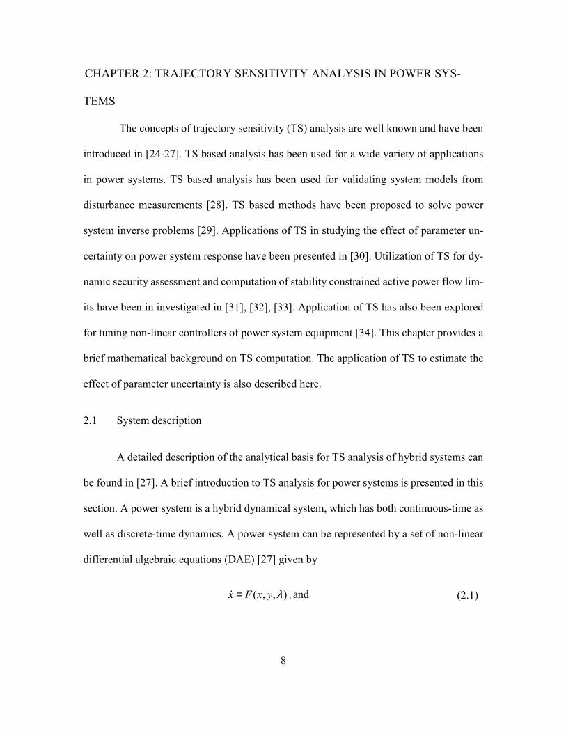
The concepts of trajectory sensitivity (TS) analysis are well known and have been
introduced in [24-27]. TS based analysis has been used for a wide variety of applications
in power systems. TS based analysis has been used for validating system models from
disturbance measurements [28]. TS based methods have been proposed to solve power
system inverse problems [29]. Applications of TS in studying the effect of parameter un-
certainty on power system response have been presented in [30]. Utilization of TS for dy-
namic security assessment and computation of stability constrained active power flow lim-
its have been in investigated in [31], [32], [33]. Application of TS has also been explored
for tuning non-linear controllers of power system equipment [34]. This chapter provides a
brief mathematical background on TS computation. The application of TS to estimate the
effect of parameter uncertainty is also described here.
2.1 System description
A detailed description of the analytical basis for TS analysis of hybrid systems can
be found in [27]. A brief introduction to TS analysis for power systems is presented in this
section. A power system is a hybrid dynamical system, which has both continuous-time as
well as discrete-time dynamics. A power system can be represented by a set of non-linear
differential algebraic equations (DAE) [27] given by
),,( λyxFx =& , and (2.1)

9
≥=<=
+
−
0),,(0),,(
0),,(0),,(
λλλλ
yxS for yxG
yxS for yxG, (2.2)
where,
x ∈ ℝn is a vector of state variables
y ∈ ℝm is a vector of algebraic variables
λ ∈ ℝp is a vector of parameters that may be subject to change
F: ℝm+n+p→ ℝn is the set of differential equations describing the evolution of the power
system state variables
G: ℝm+n+p→ ℝm is the set of algebraic equations. The + and – superscripts denote the pre
and post switching conditions
S: ℝm+n+p→ ℝl is the set of algebraic equations that define the switching conditions in
power systems
In the context of power systems, x includes the machine state variables like rotor
angles, angular speed, flux linkages and all associated controller state variables. y includes
the network algebraic variables like bus voltage magnitudes and angles. λ includes the var-
ious parameters that are used while representing the power system elements at a certain
operating condition. The parameters in a power system problem can be the machine im-
pedances, line and transformer impedances, load parameters, generator outputs, shunt re-
actance, and controller set points, to name a few. These parameters can greatly influence
the response of a power system to an event like a fault or a large load or generation change.
S defines the conditions when switching actions occur in models. Examples of switching
events would be the switching of a contactor, tripping of a component by a relay or the

10
transition of an induction motor from a running state to a stall state. It should be noted that
the model described by (2.1) and (2.2) does not adequately capture events where discrete
jumps occur in the state variables. A differential algebraic impulse system (DAIS) repre-
sentation has been suggested in [29] to account for such jumps. Nevertheless, the model
described by (2.1) and (2.2) is adequate for the purpose of this study since the events lead-
ing to discrete jumps in state variables are not pursued in this research work.
2.2 Numerical evaluation of trajectory sensitivities
The trajectory sensitivities can be evaluated either numerically or analytically. In
the numerical approach to sensitivity evaluation, the finite differencing method is used
[35]. The finite differencing method is based on the Taylor’s theorem [35]. The partial
derivatives can be computed by using a forward difference or a central difference method.
In the forward difference method [35], the partial derivatives are computed by
ελελ
λλ ),(),(),( txtxtx −+≈
∂∂
. (2.3)
In the central difference method [35], the partial derivatives are computed by
εελελ
λλ
2
),(),(),( −−+≈∂
∂ txtxtx, (2.4)
where, ε is a small perturbation and t is the time. A detailed discussion on the different
finite difference methods can be found in [35]. For an infinitesimal small perturbation ε,
the finite differencing methods provide a reasonably accurate estimate of the partial deriv-
atives. Between the two finite difference methods described, the central difference method
11
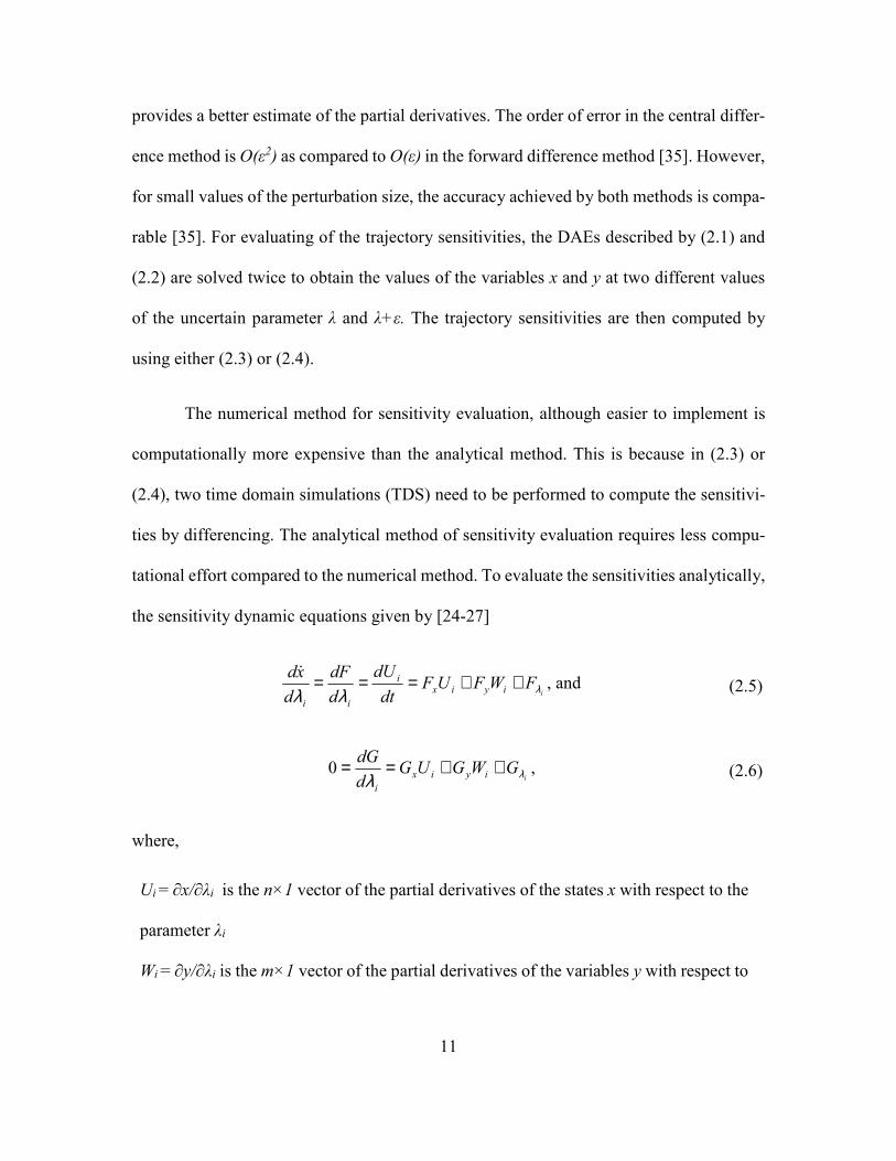
provides a better estimate of the partial derivatives. The order of error in the central differ-
ence method is O(ε2) as compared to O(ε) in the forward difference method [35]. However,
for small values of the perturbation size, the accuracy achieved by both methods is compa-
rable [35]. For evaluating of the trajectory sensitivities, the DAEs described by (2.1) and
(2.2) are solved twice to obtain the values of the variables x and y at two different values
of the uncertain parameter λ and λ+ε. The trajectory sensitivities are then computed by
using either (2.3) or (2.4).
The numerical method for sensitivity evaluation, although easier to implement is
computationally more expensive than the analytical method. This is because in (2.3) or
(2.4), two time domain simulations (TDS) need to be performed to compute the sensitivi-
ties by differencing. The analytical method of sensitivity evaluation requires less compu-
tational effort compared to the numerical method. To evaluate the sensitivities analytically,
the sensitivity dynamic equations given by [24-27]
iFWFUF
dt
dU
d
dF
d
xdiyix
i
ii
λλλ++===
&, and (2.5)
iGWGUG
d
dGiyix
i
λλ++==0 , (2.6)
where,
Ui = ∂x/∂λi is the n×1 vector of the partial derivatives of the states x with respect to the
parameter λi
Wi = ∂y/∂λi is the m×1 vector of the partial derivatives of the variables y with respect to

12
the parameter λi
Fx is the n×n matrix of the partial derivatives of F with respect to the state variables x
Fy is the n×m matrix of the partial derivatives of F with respect to the algebraic varia-
bles y
Fλi is the n×1 vector of partial derivative of F with respect to the ith parameter λi
Gx is the m×n matrix of the partial derivatives of G with respect to the state variables x
Gy is the m×m matrix of the partial derivatives of G with respect to the algebraic vari-
ables y
Gλi is the m×1 vector of the partial derivatives of G with respect to the ith parameter λi
The sensitivity dynamic equations (2.5) and (2.6) are solved simultaneously with
the system equations (2.1) and (2.2) to evaluate the sensitivities Ui and Vi for a change in
the ith parameter λi. While evaluating the DAEs given by (2.1) and (2.2) using an implicit
integration routine like the trapezoidal method [36], the updated variables for the next time
step is found by solving
0))),(),(()),(),(((2
)()( =+∆+∆+∆−−∆+ λλ tytxFttyttxFt
txttx , and (2.7)
0)),(),(( =∆+∆+ λttyttxG , (2.8)
where, t is the time and ∆t is the time step of integration. Since (2.7) and (2.8) are a set of
non-linear equations, an iterative technique like the Newton-Raphson method is used to
solve for x(t+∆t) and y(t+∆t) at each time step of the integration. The Jacobian required
for solving (2.7) and (2.8) is given by

13
∆∆−
yx
yx
GG
tF
tFI
22 . (2.9)
To augment the computation of trajectory sensitivities with the TDS routine, (2.5)
and (2.6) can are rewritten as
0))(),(( === tWtUFdt
dU
d
xdiinew
i
iλ&
, and (2.10)
0))(),(( =tWtUG iinew , (2.11)
where, Fnew and Gnew are the right hand sides of (2.5) and (2.6) respectively. Using the
trapezoidal rule (2.10) and (2.11) are rewritten as
)))(),(())(),(((2
)()( tWtUFttWttUFt
tUttU iinewiinewii +∆+∆+∆+=∆+ , and (2.12)
0))(),(( =∆+∆+ ttWttUG ii . (2.13)
(2.12) and (2.13) can be expanded and written as a linear matrix equation given by
∆+−
∆++++∆+
=
∆+∆+
∆+∆+
∆+∆−∆+∆−
)(
))()()()()()((2
)(
)(
)(
)()(
)(2
)(2
ttG
ttFtFtWtFtUtFt
tU
ttW
ttU
ttGttG
ttFt
ttFt
I
i
iiiyixi
i
i
yx
yx
λ
λλ
. (2.14)
The generic form of (2.14) for hybrid dynamical systems can also be found in [27].
It can be seen that Fx, Fy, Gx and Gy required to solve the linear matrix equation (2.29) are
already computed during the TDS. All the terms in (2.14) except Ui(t+∆t), and Wi(t+∆t)

14
are known and the unknown terms can be found by factorizing the right hand side of (2.14)
and solving the linear matrix equation. Furthermore, the matrix in the right hand side of
(2.14) is same as the Jacobian (2.9). Therefore, the factors of the Jacobian given by (2.9)
that are computed in the TDS routine can be used directly. The only additional computa-
tional effort required in this method is to evaluate the vectors Fλ and Gλ in (2.14), which
are sparse. Therefore, the evaluation of the trajectory sensitivities by the analytical method
does not require any major additional computational effort. The implementation of the TS
routine in PSAT has been described in [37].
The sensitivities Ui and Wi are discontinuous at the switching events described by
S in (2.2). Reference [27] provides details on the calculation of the switching conditions
and the sensitivities at these switching events. The sensitivity dynamic equations for dif-
ferent parameter changes are independent of each other and hence amenable to parallel
computation. The use of parallel computation results in additional savings in computation
time. References [37] and [38] describe the implementation of TS analysis in power sys-
tems using cluster computing.
2.3 Estimating the effect of parameter uncertainty
Once the trajectory sensitivities are evaluated, the impact of the change in a param-
eter value on the system trajectories can be studied without the need for multiple TDSs.
For a change in the magnitude of a parameter λi the perturbed trajectories can be estimated
by a linear approximation as
15
i
i
oldest
txtxtx λ
λ∆
∂∂+= )(
)()( , and (2.15)
i
i
oldest
tytyty λ
λ∆
∂∂+= )(
)()( , (2.16)
where, x(t)old, and y(t)old are the base case trajectories, x(t)est, and y(t)est are the estimated
trajectories and ∆λi the change in λi for which the trajectories are being estimated
The linear approximation of trajectories is reasonably accurate when the parameter
perturbation sizes are small. If the perturbation sizes are large, truncation error associated
with the omission higher order terms of the Taylor series arises. It is therefore important to
evaluate the limit of perturbation size for which linear approximations hold. The evaluation
of perturbation size is a topic in itself and has been discussed in a later chapter.
2.4 Summary
This chapter presented an introduction to TS analysis and its applications in power
system. A discussion of both the numerical method and the analytical method of evaluating
the sensitivities is presented here. The implementation of the analytical approach along
with an implicit integration based TDS is presented here. In addition, it is shown that the
analytical method of TS evaluation is computationally less burdensome as compared to the
numerical method.

16
CHAPTER 3: APPLICATION OF TRAJECTORY SENSITIVITY TO ANA-
LYZE LOAD PARAMETER UNCERTAINTY
In power system studies, loads are modeled as an aggregation of different types of
consumer loads at the distribution substation [11], [13-16]. The WECC composite load
model developed by the WECC MVWG [13], [14] is one such load model that has been
widely incorporated in several commercial power system simulators [22], [23]. Since the
WECC composite load is an aggregated load model, one of the main challenges is in de-
termining the exact composition of the load. Furthermore, the load parameter estimation
process, which primarily relies on surveys and measurements, introduces additional varia-
bility [15], [16]. It is therefore important to assess the impact of load composition and
parameter uncertainty on the dynamic response of the system. TS analysis provides a suit-
able avenue to perform such assessments. In addition to estimating the change in the sys-
tem response, TS analysis serves to identify the most important load parameters, which are
consequential from a system performance viewpoint.
This chapter describes the composite load model and the application of TS analysis
for studying load parameter uncertainty. In the following sections, the composite load
model is described in details and the sensitivities of some of the important composite load
model parameters are studied. Furthermore, the application of TS to estimate the system
response to a change in a load parameter is demonstrated here.
3.1 The WECC composite load model
The WECC composite load model represents an aggregation of consumer loads at
the substation level. Figure 3.1 shows the implementation of the WECC composite load

17
model in GE-PSLF a commercially available power system simulator [22]. The WECC
composite load model is referred to as ‘cmpldw’ in the GE-PSLF model library [22]. A
detailed description of the ‘cmpldw’ model and the associated parameters can be found in
[22].
To ensure flexibility in terms of the implementation of various models and algo-
rithms, PSAT a MATLAB based open source power system simulator was used for this
research [39], [40]. PSAT is a positive sequence power flow and electromechanical transi-
ent simulator like GE-PSLF. A composite load model based on the GE-PSLF ‘cmpldw’
was created in PSAT. Figure 3.2 shows the composite load model developed for the study
in PSAT. The motors are labeled as A, B, C and D since the same nomenclature is adopted
by most commercial power system simulators [22], [23]. The description of the various
components shown in Figure 3.2 is as follows:
1. Motor A is the cumulative representation of the motors with high inertia
connected to the distribution bus.
2. Motor B is the cumulative representation of the motors with low inertia con-
nected to the distribution bus.
3. Motor C is the cumulative representation of the motors connected to the
distribution bus with low inertia, which trip under low voltage condition
with a pre-specified time delay.
4. Motor D is the cumulative representation of the single-phase induction mo-
tor (SPIM) driven A/C connected to the distribution bus.

18
5. Electronic load: The electronic load is a constant PQ load operating at a
constant power factor. The load disconnects and reconnects linearly when
the terminal voltage drops or rises above set thresholds respectively [22].
6. Static load: The static load is represented by the standard ZIP load model
[22].
Motor A, motor B and motor C are modeled as three-phase double cage induction
motors with a quadratic load torque versus speed characteristics [6], [40]. The dynamics of
the three-phase induction motors are represented by differential equations and can be found
in [40]. Motor A, motor B and motor C are represented by the ‘Order V’ induction motor
model in PSAT [40]. The ‘Order V’ induction motor model in PSAT is similar the ‘mo-
torw’ model in the PSLF model library [22].
Figure 3.1 The composite load model ‘cmpldw’ in GE-PSLF [22]
19
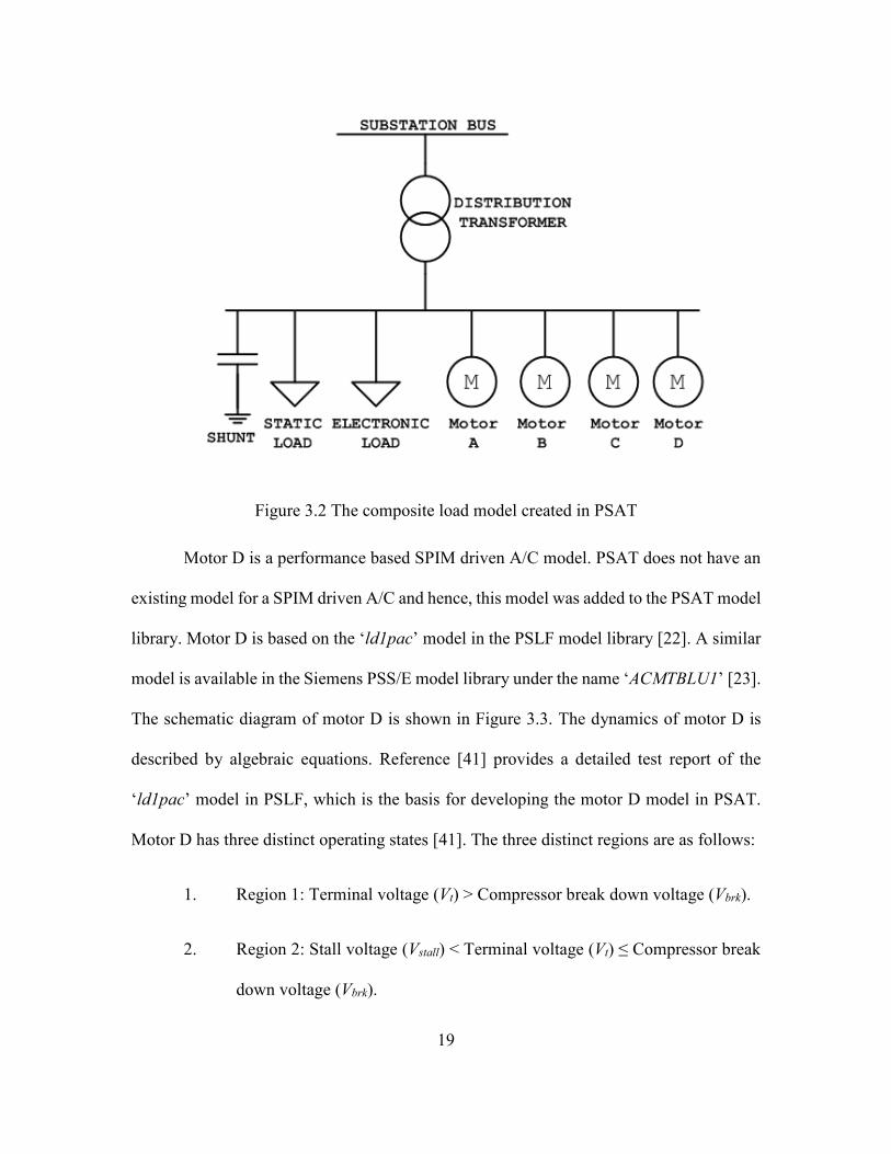
Figure 3.2 The composite load model created in PSAT
Motor D is a performance based SPIM driven A/C model. PSAT does not have an
existing model for a SPIM driven A/C and hence, this model was added to the PSAT model
library. Motor D is based on the ‘ld1pac’ model in the PSLF model library [22]. A similar
model is available in the Siemens PSS/E model library under the name ‘ACMTBLU1’ [23].
The schematic diagram of motor D is shown in Figure 3.3. The dynamics of motor D is
described by algebraic equations. Reference [41] provides a detailed test report of the
‘ld1pac’ model in PSLF, which is the basis for developing the motor D model in PSAT.
Motor D has three distinct operating states [41]. The three distinct regions are as follows:
1. Region 1: Terminal voltage (Vt) > Compressor break down voltage (Vbrk).
2. Region 2: Stall voltage (Vstall) < Terminal voltage (Vt) ≤ Compressor break
down voltage (Vbrk).

20
3. Region 3:Terminal voltage (Vt) ≤ Stall voltage (Vstall)
Region 1 and region 2 are running states, while region 3 represents the stalled con-
dition of the SPIM driven A/C. The active and the reactive power consumed by the SPIM
driven A/C in the different operating states are as follows [41]:
Region 1: Terminal voltage (Vt) > Compressor break down voltage (Vbrk)
The active and reactive power consumed by the SPIM in region 1 is given by
0
1
)(1 PVVKpPbrkt
Np
run += − , and (3.1)
0
1
)(1 QVVKqQbrkt
Nq
run += − , (3.2)
where,
Prun is the active power consumed by motor D in the running state
Qrun is the reactive power consumed by motor D in the running state
Kp1 is the active power coefficient in region 1
Kq1 is the reactive power coefficient region 1
Np1 is the active power exponent in region 1
Nq1 is the reactive power exponent in region 1
Vt is the terminal voltage of the machine
Vbrk is the breakdown voltage of the A/C
P0 and Q0 are given by
( ) 1
0 111Np
brkVKpP −−= , and (3.3)
)(111 1
2
0 brk
Nq
VKqpf
pfQ −−
−= ,
(3.4)
where, pf is the power factor
21
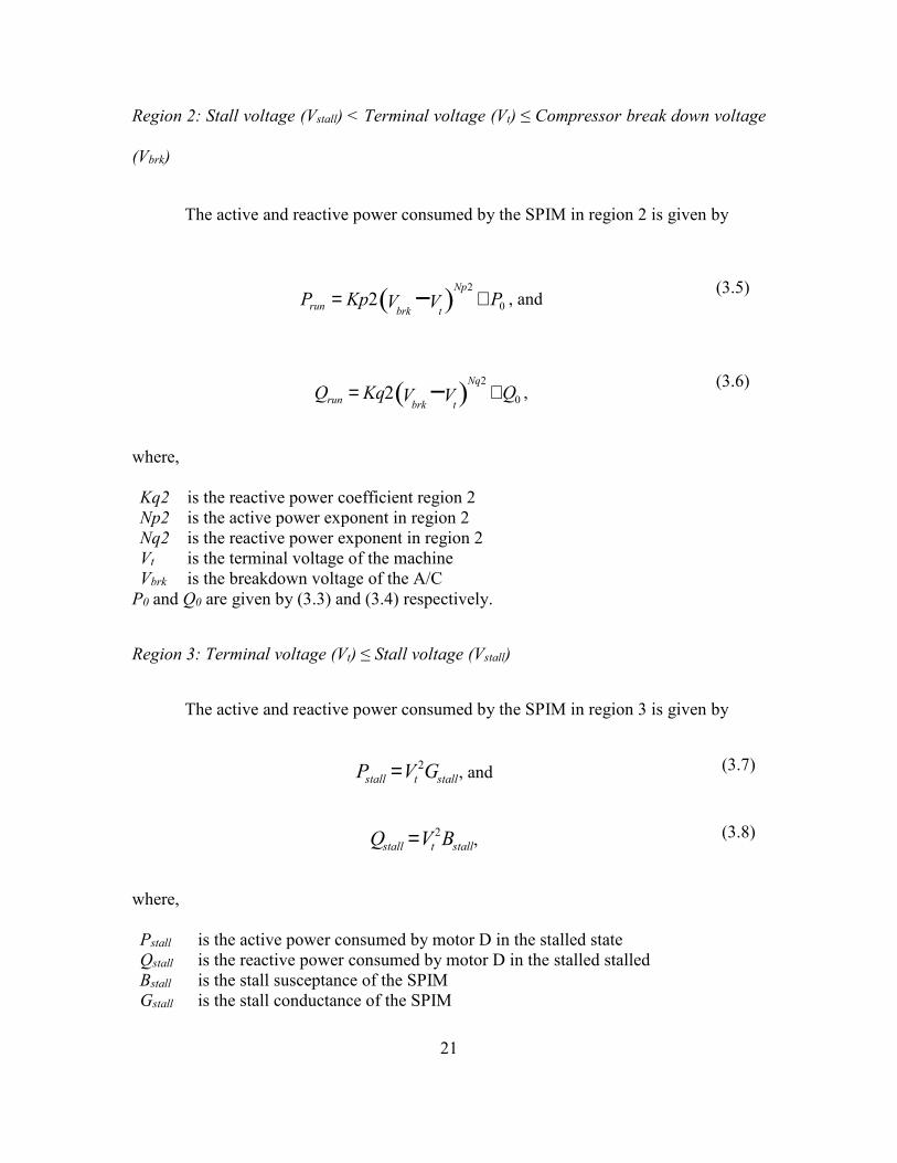
Region 2: Stall voltage (Vstall) < Terminal voltage (Vt) ≤ Compressor break down voltage
(Vbrk)
The active and reactive power consumed by the SPIM in region 2 is given by
0
2
)(2 PVVKpPtbrk
Np
run += − , and (3.5)
0
2
)(2 QVVKqQtbrk
Nq
run += − , (3.6)
where,
Kq2 is the reactive power coefficient region 2
Np2 is the active power exponent in region 2
Nq2 is the reactive power exponent in region 2
Vt is the terminal voltage of the machine
Vbrk is the breakdown voltage of the A/C
P0 and Q0 are given by (3.3) and (3.4) respectively.
Region 3: Terminal voltage (Vt) ≤ Stall voltage (Vstall)
The active and reactive power consumed by the SPIM in region 3 is given by
stalltstall GVP 2= , and (3.7)
stalltstall BVQ 2= , (3.8)
where,
Pstall is the active power consumed by motor D in the stalled state
Qstall is the reactive power consumed by motor D in the stalled stalled
Bstall is the stall susceptance of the SPIM
Gstall is the stall conductance of the SPIM
22
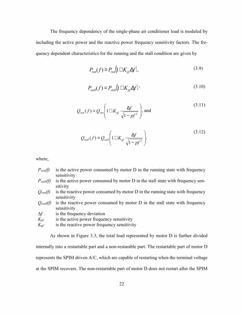
The frequency dependency of the single-phase air conditioner load is modeled by
including the active power and the reactive power frequency sensitivity factors. The fre-
quency dependent characteristics for the running and the stall condition are given by
( )fKPfP pfrunrun ∆+= 1)( , (3.9)
( )fKPfP pfstallstall ∆+= 1)( ’ (3.10)
−∆+=
211)(
pf
fKQfQ qfrunrun
, and
(3.11)
−∆+=
211)(
pf
fKQfQ qfstallstall
,
(3.12)
where,
Prun(f) is the active power consumed by motor D in the running state with frequency
sensitivity
Pstall(f) is the active power consumed by motor D in the stall state with frequency sen-
sitivity
Qrun(f) is the reactive power consumed by motor D in the running state with frequency
sensitivity
Qstall(f) is the reactive power consumed by motor D in the stall state with frequency
sensitivity
∆f is the frequency deviation
Kpf is the active power frequency sensitivity
Kqf is the reactive power frequency sensitivity
As shown in Figure 3.3, the total load represented by motor D is further divided
internally into a restartable part and a non-restarable part. The restartable part of motor D
represents the SPIM driven A/C, which are capable of restarting when the terminal voltage
at the SPIM recovers. The non-restartable part of motor D does not restart after the SPIM
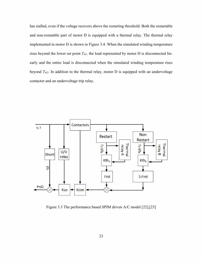
23
has stalled, even if the voltage recovers above the restarting threshold. Both the restartable
and non-restatable part of motor D is equipped with a thermal relay. The thermal relay
implemented in motor D is shown in Figure 3.4. When the simulated winding temperature
rises beyond the lower set point Tth1, the load represented by motor D is disconnected lin-
early and the entire load is disconnected when the simulated winding temperature rises
beyond Tth2. In addition to the thermal relay, motor D is equipped with an undervoltage
contactor and an undervoltage trip relay.
Figure 3.3 The performance based SPIM driven A/C model [22],[23]

24
Figure 3.4 The thermal relay model in motor D [22], [23]
3.2 Case description
The WECC 2012 high summer (HS) case has been used in this research to perform
the load parameter sensitivity study. Accordingly, the power flow file for the WECC sys-
tem was converted appropriately for use in PSAT. Details of the WECC 2012 HS case can
be found in APPENDIX A. The loads in the system were represented by the composite
load model developed for PSAT. It should be noted that the original WECC 2012 HS case,
available through the WECC website, does not use a composite load model to represent
the loads. The composite load model was later added to the WECC 2012 HS case sepa-
rately. The composition of the composite load model connected at a load bus was deter-
mined based on the season, hour of the day and the region where the load bus is located.
The region where the load bus is located can be ascertained by the long identifier associated
with every load bus provided in the WECC power flow data. APPENDIX A lists the com-
position of the load at different buses based on the long identifier, which is used for the
work presented in this dissertation. In addition, the load buses have been renamed arbitrar-
ily to mask the identity of the actual buses in the system.
25
3.3 Parameter sensitivities during a large disturbance
The work done in this research particularly focuses on the parameters of the motor
D part of the WECC composite load described in chapter 2 [42]. Motor D, which represents
a SPIM driven A/C primarily responsible for the fault induced delayed voltage recovery
(FIDVR) phenomenon [43]. FIDVR is the unexpected delay in the recovery of the voltage
after the normal clearing of a fault [43]. Larger motors have higher inertia and hence do
not stall immediately after a transient voltage dip or a transient fault. Since the larger mo-
tors do not stall immediately, they have less effect on the system voltage recovery. In ad-
dition, the motor D part of the composite load model is interesting from a sensitivity anal-
ysis viewpoint because of its non-smooth nature. Although only the parameters of motor
D are examined here, the same analysis could be extended without loss of generality to any
uncertain parameter of the composite load model. The motor D component of the compo-
site load model will be referred to as SPIM in the remainder of the dissertation.
The complete list of parameters of the composite load model is provided in AP-
PENDIX A. The default values for the composite load model parameters as suggested by
GE-PSLF can be found in [22]. Table 3.1 lists some of the parameters of the SPIM used
for this research. As indicated in Table 3.1, Vstall and Tstall are used to define the condi-
tions, when the SPIM transitions from a running state to a stall state.
To simulate the FIDVR event, a three-phase 5-cycle fault was applied on one of the
major 500 kV lines in the southwestern WECC system. The fault was applied at t = 0.2 s.
The simulation was conducted with the values for the load parameters listed in Table 3.1.
26
The sensitivities of the power system state and algebraic variables to the parameters con-
sidered in Table 3.1, were computed. Two load buses, LB1 and LB2, were chosen to study
the parameter sensitivities. Figure 3.5 and Figure 3.6 show the bus voltages and the sensi-
tivities of the bus voltages to the load parameters at buses LB1 and LB2 respectively. Bus
LB1 is closer to the fault and the SPIM connected at this bus stalls immediately after the
fault is applied. This is shown in Figure 3.5(a). Bus LB2 is farther away from the fault and
the SPIM connected at this bus stalls approximately 0.6s after the fault is cleared due to
the depressed voltage. This is shown in Figure 3.6(a). The stalling of the SPIM can be seen
as a sharp dip in the voltage in both Figure 3.5(a) and Figure 3.6(a). The sharp dip in the
voltage is due to the transition of the SPIM from the running state to the stall state. Once
stalled, the active and the reactive power consumption of SPIM increases abruptly depend-
ing on the Rstall and the Xstall respectively [41], [42]. The stalling of the SPIM at the load
buses results in a delayed voltage recovery in the area of interest.
A few important observations can be made from Figure 3.5 and Figure 3.6 [42].
The negative value of the voltage sensitivity to Fmd in Figure 3.5(b) and Figure 3.6(b)
indicates that that an increase in the percentage of SPIM (Fmd) in the load composition at
the buses will result in a poorer voltage recovery due to the fault. This is expected since a
larger number of stalled SPIMs exacerbate the FIDVR phenomenon. Conversely, increas-
ing the stall resistance and reactance (Rstall and Xstall) causes the SPIM to consume less
power in the stalled state. Therefore increasing Rstall and Xstall aids the voltage recovery
process. This can be interpreted from the positive values of the voltage sensitivities to
Rstall and Xstall [42].

27
The sensitivity of bus voltages to Tstall and Vstall are different from the sensitivity
behavior to Rstall and Xstall. Figure 3.5(c) and Figure 3.6(c) show the sensitivity of bus
voltages to Tstall and Vstall. From Figure 3.6(c) it can be seen that a change in Tstall and
Vstall affects the voltage at bus LB2 only at the time of stall. As time progresses, the sen-
sitivity of bus voltage to these parameters diminish to zero. From Figure 3.5(c) a similar
conclusion can be drawn about the sensitivity of the voltage at bus LB1 to Tstall. However,
unlike in Figure 3.6(c), the voltage at bus LB1 is not sensitive to Vstall in Figure 3.5(c).
The bus LB1 being electrically closer to the fault location experiences a larger dip in volt-
age due to the fault. As shown in Figure 3.5(a), the voltage drops sharply below 0.5 pu at
the instant of the fault and remains close to 0.5 pu till the fault is cleared. The fault causes
the voltage at the bus to drop below the SPIM voltage threshold Vstall instantaneously.
Small changes in Vstall do not appreciably change the time instant when the SPIM stalls.
Therefore, the voltage at bus LB1 is not sensitive to Vstall. However, at bus LB2, which is
farther away from the fault, the voltage drops gradually below the SPIM stall conditions
(around 0.8s in Figure 3.6(c)). Due to the gradual descent of the voltage into the stall con-
dition, a change in Vstall significantly changes the time instant when the SPIM stalls.
Therefore, the magnitude of the sensitivity of voltage to Vstall at bus LB2 is considerably
high at the time instant when the SPIM connected at this bus stalls.
The sensitivities of the voltage to the SPIM stall parameters are high at the time of
stall and decrease rapidly as time progresses. This is expected since the stall parameters
Vstall and Tstall only affect the time instant and the duration taken for the SPIM to transi-
tion from a running state to a stall state. Vstall and Tstall are not present in the algebraic
equations describing the power consumption of the SPIM in the performance model. In

28
terms of the mathematical formulation of the composite load model, Vstall and Tstall are
present only in S of (2.2), which are the algebraic equations defining the switching condi-
tions of the SPIM. On the other hand, Rstall, Xstall, Fmd are present only in G of (2.2)
which are the algebraic equations defining the behavior of the SPIM in the running and
stalled conditions.
Table 3.1 Parameters of motor D examined in this study
Parameter Value Description
Fmd - Fraction of motor D (SPIM) load in composite load
model (in pu)
Rstall 0.124 pu Stall conductance in pu
Xstall 0.114 pu Stall susceptance in pu
Tstall 0.033 s Time after which the SPIM stalls due to under-voltage
Vstall 0.7 pu Voltage below which SPIM stalls
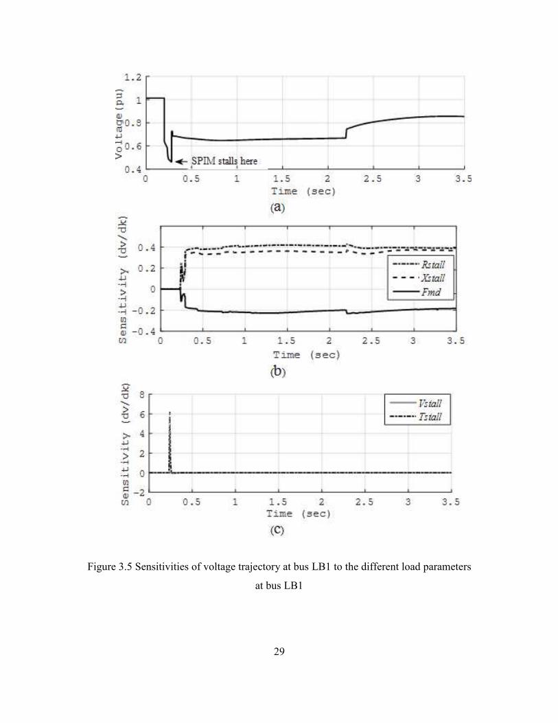
29
Figure 3.5 Sensitivities of voltage trajectory at bus LB1 to the different load parameters
at bus LB1
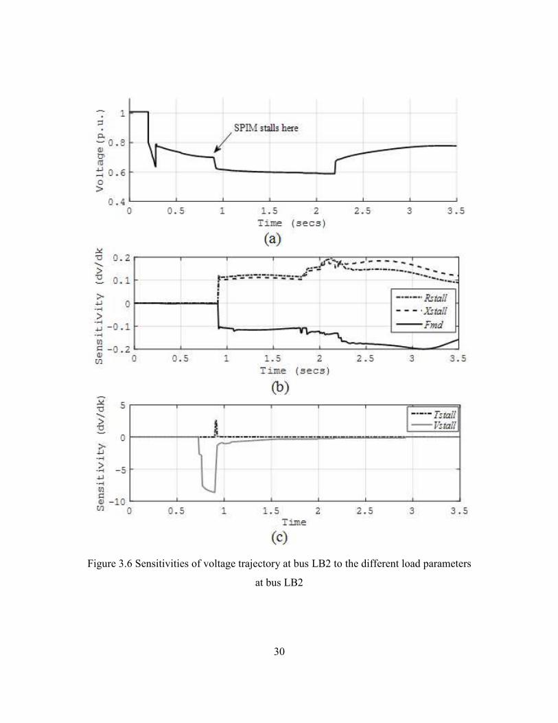
30
Figure 3.6 Sensitivities of voltage trajectory at bus LB2 to the different load parameters
at bus LB2
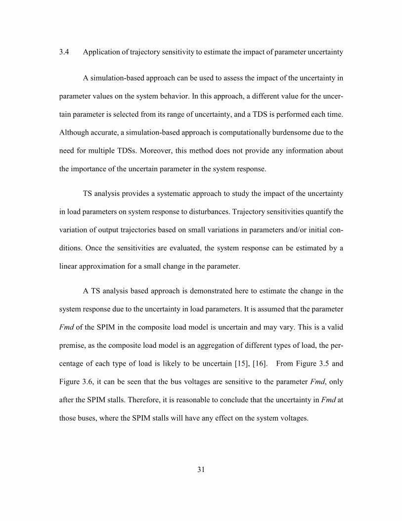
31
3.4 Application of trajectory sensitivity to estimate the impact of parameter uncertainty
A simulation-based approach can be used to assess the impact of the uncertainty in
parameter values on the system behavior. In this approach, a different value for the uncer-
tain parameter is selected from its range of uncertainty, and a TDS is performed each time.
Although accurate, a simulation-based approach is computationally burdensome due to the
need for multiple TDSs. Moreover, this method does not provide any information about
the importance of the uncertain parameter in the system response.
TS analysis provides a systematic approach to study the impact of the uncertainty
in load parameters on system response to disturbances. Trajectory sensitivities quantify the
variation of output trajectories based on small variations in parameters and/or initial con-
ditions. Once the sensitivities are evaluated, the system response can be estimated by a
linear approximation for a small change in the parameter.
A TS analysis based approach is demonstrated here to estimate the change in the
system response due to the uncertainty in load parameters. It is assumed that the parameter
Fmd of the SPIM in the composite load model is uncertain and may vary. This is a valid
premise, as the composite load model is an aggregation of different types of load, the per-
centage of each type of load is likely to be uncertain [15], [16]. From Figure 3.5 and
Figure 3.6, it can be seen that the bus voltages are sensitive to the parameter Fmd, only
after the SPIM stalls. Therefore, it is reasonable to conclude that the uncertainty in Fmd at
those buses, where the SPIM stalls will have any effect on the system voltages.

32
To simulate a large grid disturbance, a three-phase 5-cycle fault was applied on one
of the major 500 kV lines in the southwestern WECC system. This is the same disturbance
considered in the preceding section. It was observed that the SPIM component of the com-
posite load connected at 20 load buses, located close to the fault, stalled due the voltage
dip. The uncertainty in Fmd was considered at these 20 load buses. Since an increase in
Fmd results in poorer voltage recovery, a positive increase in the parameter Fmd is of con-
cern from a power system planning viewpoint. It is therefore assumed that the parameter
Fmd at the selected load buses may increase by 5%. The change in Fmd is referred to as
ΔFmd in the rest of this report. The sensitivities were evaluated using (2.5)-(2.6) and the
estimated trajectories for the system voltages were computed using (2.15) and (2.16). Fig-
ure 3.7 and Figure 3.8 show the estimated voltage trajectory at buses LB1 and LB3 respec-
tively, for a ΔFmd of 5% at the 20 selected buses. From Figure 3.7 and Figure 3.8 it can be
seen that the estimated trajectory provides a reasonably accurate estimate of the actual
voltage trajectory. The actual voltage trajectory is obtained by repeating the TDS by chang-
ing the parameter Fmd. In addition, Figure 3.9 to Figure 3.11 shows the actual and esti-
mated trajectories of the voltage, frequency and the rotor angle at a generator bus GB1 in
the area of interest. From the simulation studies, it can be seen that, a TS based method can
be used to estimate the change in the system response to a parameter change without the
need for repeated TDSs.
3.5 Comparison of computation time with repeated TDS
Table 3.2 presents the time required to run the various routines for trajectory esti-
mation. In addition, the total time required to estimate the trajectories using the TS based
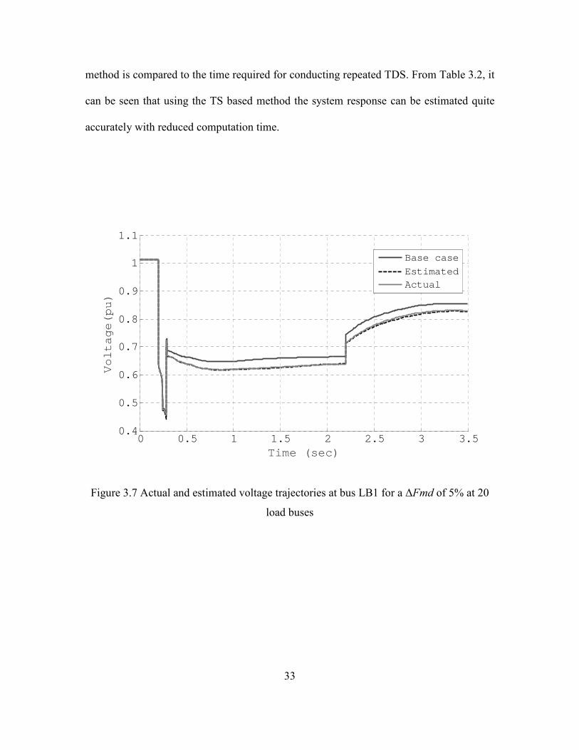
33
method is compared to the time required for conducting repeated TDS. From Table 3.2, it
can be seen that using the TS based method the system response can be estimated quite
accurately with reduced computation time.
Figure 3.7 Actual and estimated voltage trajectories at bus LB1 for a ΔFmd of 5% at 20
load buses
0 0.5 1 1.5 2 2.5 3 3.50.4
0.5
0.6
0.7
0.8
0.9
1
1.1
Time (sec)
Voltage(pu)
Base case
EstimatedActual

34
Figure 3.8 Actual and estimated voltage trajectories at bus LB3 for a ΔFmd of 5% at 20
load buses
Figure 3.9 Actual and estimated voltage trajectories at bus GB1 for a ΔFmd of 5% at 20
load buses
0 0.5 1 1.5 2 2.5 3 3.50.4
0.5
0.6
0.7
0.8
0.9
1
1.1
Time (sec)
Voltage(pu)
Base case
EstimatedActual
0 0.5 1 1.5 2 2.5 3 3.5
0.65
0.7
0.75
0.8
0.85
0.9
0.95
1
1.05
Time (sec)
Voltage (pu)
Base caseEstimatedActual

35
Figure 3.10 Actual and estimated frequency trajectories at bus GB1 for a ΔFmd of 5% at
20 load buses
Figure 3.11 Actual and estimated relative rotor angle trajectories at bus GB1 for a ΔFmd
of 5% at 20 load buses
0 0.5 1 1.5 2 2.5 3 3.559.9
60
60.1
60.2
60.3
Time (sec)
Frequency (Hz)
Base case
EstimatedActual
0 0.5 1 1.5 2 2.5 3 3.5
1.4
1.6
1.8
2
2.2
2.4
2.6
Time (sec)
Relative rotor angle (deg)
Base caseEstimatedActual

36
Table 3.2 Simulation metrics for TS analysis and repeated TDS in PSAT
Solution metrics (3.5 sec simulation with 0.0083 sec time step)
Time domain simulation
(Evaluating base case including
storing the Jacobian entries)
789.201
sec Needs to be done once
Calculate initial values of sensitivi-
ties 1.708 sec To be done in parallel
Calculate the sensitivities 143.72 sec To be done in parallel
Create the final trajectory 32.29 sec
Can be done in parallel for dif-
ferent values of delta change
Total time for TS based estimation 966.919 sec
Total time for two repeated TDS 1575.402 sec
Savings in computation time 608.483 sec
3.6 Summary
This chapter demonstrated the application of TS to study the impact of load param-
eter uncertainty on the dynamic response of the system. The sensitivities of a few selected
parameters of the SPIM component of the composite load model were discussed. The
application of TS to study parameter uncertainty was demonstrated on the WECC system,
which is a realistic large power system. The results show that the TS based estimation of
the system response is reasonably accurate for the considered uncertainty in the particular
load parameter. Furthermore, the chapter compares the computation time of the TS based
method to the repeat TDS method for estimating the effect of parameter uncertainty. The
comparison results indicate that application of the TS based method results in a substantial
savings in computational effort.
37
CHAPTER 4: PARAMETER SENSITIVITY STUDIES IN POWER SYSTEMS
WITH NON-SMOOTH LOAD BEHAVIOR
TS based methods rely on linear approximations based on the first order partial
derivatives of the state and algebraic variables with respect to the parameters of interest. It
is therefore important to analyze the limit of the perturbation size for which TS based esti-
mations are reasonably accurate. Trajectory estimation using linear approximation has been
found to be effective for small perturbations. References [32], [33] have reported that the
linear approximation is reasonably accurate when the power system is far from instability.
However, the non-smooth nature of the SPIM part of the composite load model presents
additional challenges for trajectory estimation. This chapter presents a discussion on the
limitations of perturbation sizes while using TS based analysis for power system studies
with non-smooth load models. Similar analysis could be extended to find perturbation size
limits while dealing with any other non-smooth component model.
4.1 Effect of switching hypersurface on TS analysis in hybrid dynamical systems
Consider the description of the power system given by (2.1)-(2.2) in chapter 2. The
equations are repeated here for convenience.
),,( λyxFx =& , and (4.1)
≥=<=
+
−
0),,(0),,(
0),,(0),,(
λλλλ
yxS for yxG
yxS for yxG. (4.2)
The power system is a hybrid dynamical system where the switching hypersurface
is defined by
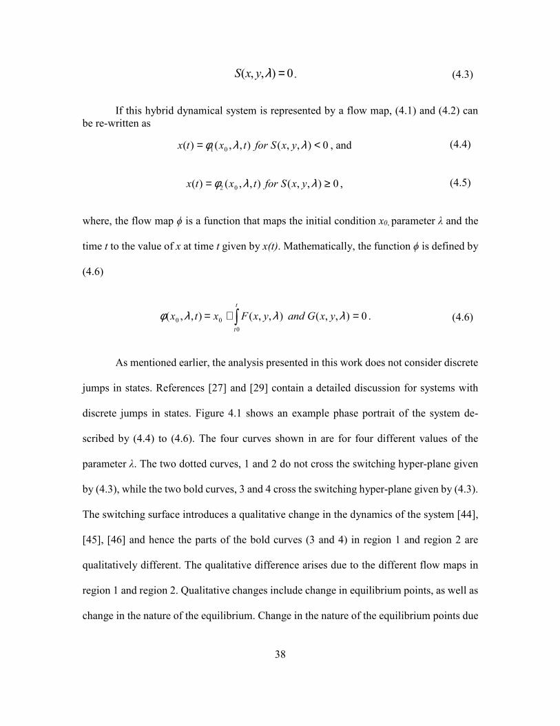
38
0),,( =λyxS . (4.3)
If this hybrid dynamical system is represented by a flow map, (4.1) and (4.2) can
be re-written as
0),,(),,()( 01 <= λλφ yxS for txtx , and (4.4)
0),,(),,()( 02 ≥= λλφ yxS for txtx , (4.5)
where, the flow map ϕ is a function that maps the initial condition x0, parameter λ and the
time t to the value of x at time t given by x(t). Mathematically, the function ϕ is defined by
(4.6)
∫ =+=t
t
yxG and yxFx tx0
00 0),,(),,(),,( λλλφ . (4.6)
As mentioned earlier, the analysis presented in this work does not consider discrete
jumps in states. References [27] and [29] contain a detailed discussion for systems with
discrete jumps in states. Figure 4.1 shows an example phase portrait of the system de-
scribed by (4.4) to (4.6). The four curves shown in are for four different values of the
parameter λ. The two dotted curves, 1 and 2 do not cross the switching hyper-plane given
by (4.3), while the two bold curves, 3 and 4 cross the switching hyper-plane given by (4.3).
The switching surface introduces a qualitative change in the dynamics of the system [44],
[45], [46] and hence the parts of the bold curves (3 and 4) in region 1 and region 2 are
qualitatively different. The qualitative difference arises due to the different flow maps in
region 1 and region 2. Qualitative changes include change in equilibrium points, as well as
change in the nature of the equilibrium. Change in the nature of the equilibrium points due

39
to such switching in discrete dynamic systems are referred to as border collision bifurca-
tions or grazing bifurcations [44], [45], [46].
Figure 4.1 Phase portrait of a hybrid dynamical system
In the context of trajectory sensitivity analysis, a linear prediction of curve 2 from
curve 1 or curve 4 from curve 3 and vice versa is possible in Figure 4.1. However, due to
the qualitative difference introduced by the switching hypersurface, a linear prediction of
curve 3 from curve 2 or vice-versa is not possible. To have linear prediction of one trajec-
tory from a nominal trajectory, both of them should traverse the same switching hyper-
surfaces in the same sequence [27], [44], [45].
4.2 Effect of non-smooth load model on linear trajectory estimation
In sensitivity studies involving the composite load model, the perturbation size for
which linear approximations are accurate, is often limited due to the non-smooth nature of
x(t)=φ1 (x,y,λ) x(t)=φ
2 (x,y,λ)
x(t0)
x1(t
f)
x2(t
f) x
3(t
f) h(x,y)=0
Region 1 Region 2
x4(t
f)
(1) (2)
(3) (4)

40
the SPIM part of the composite load model [42]. The discontinuities in the SPIM model
are due to
1. The discrete change in the SPIM active and reactive power consumption
when the SPIM transitions from a running condition to a stall condition
2. The disconnection of a SPIM from service by an undervoltage trip contactor
As discussed in the foregoing section, it is required that both the base case trajectory
and the actual trajectory to be estimated, encounter the same set of discontinuities. In ad-
dition, both the trajectories should satisfy the conditions of transversality [27]. The trans-
verality condition at the hyper-surface is given by [27] (4.7).
==
≠
⋅
∂∂
∂∂
0),(
0),(
0
yxG
yxS
y
x
y
S
x
S
&
&
. (4.7)
If the transversality condition is satisfied, then the jump conditions and the sensi-
tivities at the point of discontinuity can be calculated. The detailed description of the evo-
lution of the trajectory sensitivities at the switching hypersurfaces can be found in [27].
4.2.1 Estimation error introduced by the non-smooth load models
To elucidate the limit set on linear approximation, consider the trajectory estimation
at bus LB3. The voltage response at bus LB3 for a ΔFmd of 6% at the 20 selected buses is
estimated by using TS analysis. Figure 4.2 shows the actual and the estimated trajectories
at bus LB3. The voltage dip at bus LB3 due to the fault does not cause the SPIM connected

41
at this bus to stall in the base case. However, if the simulation is re-run after incrementing
Fmd by 6% at the 20 selected buses, the SPIM connected at this bus stalls at t = 0.9 s. The
effect of the stalling of this additional SPIM in the actual case manifests as an estimation
error beyond t = 0.9 s in Figure 4.2. From this example, it can be seen that for this particular
case the computed sensitivities do not provide an accurate estimate of the actual response
if the expected variation in Fmd is 6% or more. Nonetheless, a careful inspection of the
estimated trajectory indicates that for the considered perturbation, the estimated voltage at
bus LB3 dips below 0.7 pu for more than 0.033 s. Under this condition, the SPIM connected
at bus LB3 is expected to stall. Hence, an estimation error is expected at bus LB3. This
shows that the non-smooth nature of load models may impose stricter limits on the size of
variability that can be studied by the sensitivity based approach [42].
Although TS based analysis has been applied to systems with non-smooth models
[27], [28], [29], the occurrence and analysis of the estimation error shown in Figure 4.2 has
not been discussed at length. Most of the work presented previously assumes that both the
base case and the actual cases to be predicted encounter the same switching events for
reasonable perturbation sizes. The limit of the perturbation size for which linear analysis
holds in non-smooth systems is yet to be quantified. In the context of load sensitivity stud-
ies, it is possible that an additional switching event, like the stalling of an additional SPIM,
does not occur in power systems models where loads are lumped at buses separated by long
lines. This is typical for test cases or simplified representations of large power systems
where distributed loads are aggregated and represented at a single bus and the buses are
connected by transmission lines with relatively high impedance. The high impedance of
the connecting branches reduces the impact of a parameter change at a bus on the voltage
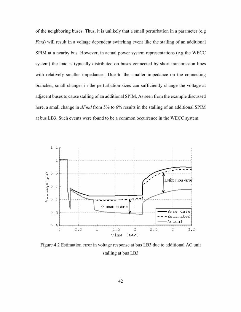
42
of the neighboring buses. Thus, it is unlikely that a small perturbation in a parameter (e.g
Fmd) will result in a voltage dependent switching event like the stalling of an additional
SPIM at a nearby bus. However, in actual power system representations (e.g the WECC
system) the load is typically distributed on buses connected by short transmission lines
with relatively smaller impedances. Due to the smaller impedance on the connecting
branches, small changes in the perturbation sizes can sufficiently change the voltage at
adjacent buses to cause stalling of an additional SPIM. As seen from the example discussed
here, a small change in ΔFmd from 5% to 6% results in the stalling of an additional SPIM
at bus LB3. Such events were found to be a common occurrence in the WECC system.
Figure 4.2 Estimation error in voltage response at bus LB3 due to additional AC unit
stalling at bus LB3

43
4.2.2 Estimation error analysis
As discussed in the previous section, the non-smooth behavior of the load model
introduces significant error in the trajectory estimation process. Therefore, it is worthwhile
to investigate
1. The magnitude of error introduced by a switching event at a bus that affects
the trajectory estimation at other buses
2. The perturbation size for which linear approximation is reasonably accurate
for power systems with non-smooth load models
Figure 4.3 shows the actual and estimated trajectory at bus LB1 for a ΔFmd of 6%
at the 20 selected buses. Bus LB1 is in the same load area as bus LB3 and hence electrically
close to each other. It should be noted that the total load represented by SPIM at bus LB3
is 35.3 MW in this case. The maximum estimation error at bus LB1 due to the stalling of
an additional SPIM at bus LB3 is less than 5%. This indicates that the error introduced by
the load model is localized in nature. The trajectory estimation at bus LB1 is repeated by
increasing the amount of load represented by SPIM at bus LB3 to 65.9 MW. Figure 4.4
shows the estimation errors at bus LB1 as the load represented by SPIM at bus LB3 is
increased. From Figure 4.4 it can be seen that an increase in the SPIM load at bus LB3
results in an increase in the estimation error at bus LB1. The increase in the error is due to
the larger discrete change in the voltage caused by the increase in the size of the SPIM load
at bus LB3. This example shows that the estimation error due to the non-smooth nature of
the load model may be localized in nature. However, the error propagation will depend on

44
the topology of the system and the magnitude of the change introduced by the additional
switching event [42].
Figure 4.3 Estimation error at bus LB1 due to stalling of an additional Motor D at bus
LB3
Figure 4.4 . Estimation error at bus LB1 for different size of SPIM at bus LB3

45
4.3 Perturbation size limit for linear accuracy including non-smooth load models
The inclusion of non-smooth load models puts additional restrictions on the limit
of linear analysis in power system. Nevertheless, such inclusions make the power system
models more realistic and the simulation results more reliable. It is therefore important to
include these models and find a limit for the perturbation size that can be used for linear
approximation of trajectories. References [37] and [38] describe a method to estimate the
maximum perturbation size for accurate linear estimation. The maximum perturbation size
is given by:
max/ SA=∆λ , (4.8)
where,
A is a constant evaluated as 1.1 experimentally [37], [38]
Δλ is the maximum perturbation size for linearity to hold
Smax is the infinite norm of the normalized sensitivity for all variables evaluated during the
base case simulation. Smax is typically high when the system is close to instability and small
otherwise. Therefore, the maximum perturbation sizes obtained are smaller for stressed
power systems and higher when power systems are well within the stability limits [37],
[38]. However, only continuous equipment models were considered in [37], [38]. To ac-
count for the non-smooth nature of the load models, the maximum perturbation size for
which the system undergoes an additional discontinuity needs to be evaluated. The com-
puted value of the perturbation size is compared to that obtained by (4.8), and the smaller
of the two is chosen as the maximum perturbation limit. It should be noted that the error
46
introduced due to linear approximation in continuous systems are a function of the higher
order terms that are neglected [35]. The error introduced due to the switching events de-
pends on the type of change introduced by the jump in the operating conditions.
The process of finding the maximum perturbation size that causes the system to
undergo an additional discontinuity can be framed as a boundary value problem (BVP)
[47]. A shooting method is a well-known approach for solving BVPs [46]. Reference [48]
provides details of the application of the shooting method to find grazing points in power
system studies. In following through with the previous analysis, computation of the maxi-
mum perturbation size of Fmd is considered here. The problem of an additional SPIM
stalling is formulated as a time difference event trigger problem [27]. To find the maximum
perturbation ΔFmd at the 20 selected buses the following assumptions are made:
Assumption 1: The perturbation size ΔFmd, at each bus should be related to each other by
some function [42]. This implies that
)()...(),( 11123112 FmdfFmdFmdfFmd FmdfFmd nn ∆=∆∆=∆∆=∆ − , (4.9)
where, n is the number of buses where a perturbation in Fmd is considered. This assumption
is needed since a single degree of freedom is available for varying parameters to find the
points where a trajectory grazes the switching conditions [32], [48]. Since the application
of trajectory sensitivity in load modeling is primarily to circumvent the effect of parameter
uncertainty, it is logical that the perturbation size in parameters will be same across differ-
ent buses or share some algebraic relation. Thus, the relation given by (4.9) would occur
47
normally in a practical problem without imposing any additional conditions. For this study
n is 20 as 20 load buses were selected to apply the perturbation ΔFmd.
Assumption 2: The bus at which the first additional SPIM stalls is known. This can be
determined by monitoring the perturbed trajectory and checking if the perturbed trajectory
meets the criteria for SPIM stall when that particular SPIM does not stall in the base case.
By using this method, the first bus where an additional SPIM stalls, can be identified. This
assumption is necessary because the perturbation size should be limited such that the volt-
age at the first bus where an additional unit stalls should just graze the stalling criteria. If
an additional SPIM stalls, it depresses the system voltage. The dip in the system voltage
may subsequently cause SPIMs connected at other buses to stall later in the simulation.
As listed in Table 3.1, the SPIM stalls if the voltage at its terminal dips below 0.7
pu and fails to recover above 0.7 pu in 0.033 secs. The shooting method is then used to find
the maximum ΔFmd such that the voltage at the particular bus dips below 0.7 pu and re-
covers above 0.7 pu in 0.033 secs. If a power system is represented as a dynamical system
given by (4.1)-(4.6), then the condition when the voltage at a bus marginally recovers with-
out the SPIMs stalling can be represented by [42]
0)(),,( 110 =− txtFmdxφ , (4.10)
0)(),,( 220 =− txtFmdxφ , (4.11)
0)),(),(( 11 =FmdtytxG , (4.12)

48
0)),(),(( 22 =FmdtytxG , (4.13)
0))(),(( 11 =tytxS , (4.14)
0))(),(( 22 =tytxS , and (4.15)
τ=− 12 tt , (4.16)
where,
ϕ defines a flow map given by (4.6)
t1, t2 represent the time instants when the switching conditions given by (4.14) and (4.15)
are satisfied
τ is the duration of time between t1and t2 required for the event to trigger
If the voltage of the bus b, with the first instance of additional SPIM stalling is
given by Vb, then (4.14)-(4.16) can be re-written as
07.0)( 1 =−tVb , (4.17)
07.0)( 2 =−tVb , and (4.18)
033.012 =− tt . (4.19)
The equations given by (4.10)-(4.16) are a set of nonlinear equations of the form

49
0)(
)(
)(
)(
2
1
2
1
2
1
=
t
t
Fmd
ty
ty
tx
tx
f .
(4.20)
(4.10)- (4.16) can be solved iteratively by using the Newton-Raphson (NR) method.
The generic form of the Jacobian required for solving time difference event trigger prob-
lems can be found in [42], [48]. In this specific problem, the Jacobian required to solve
(4.11) is given by [42]
−
∂∂−
∂∂−
1100000
00000
00000
0000
0000
),,(0000
0),,(000
22
11
222
111
2
2
1
1
tytx
tytx
ttytx
ttytx
tt
tt
SS
SS
GGG
GGG
yxFx
I
yxFx
I
λ
λ
λλ
λλ
,
where, Fmd=λ and 07.0)(),( =−= tVyxS b .
(4.21)
From (4.21) it can be seen that all the elements of the Jacobian are already available
as a by-product of the TDS and TS analysis routines. No additional computations are re-
quired for setting up the problem defined by (4.10)-(4.16). However, at every step of the
NR iteration, a time domain simulation needs to be performed to solve the flow maps in
(4.10) and (4.11). In addition, appropriate starting values for the solution variables need to

50
be determined before starting the NR iteration. To find the appropriate initial conditions
for the shooting method the following comments are in order [42]:
1. The initial values xo and yo for computing the flows remain unchanged
within iterations.
2. The initial values of Fmd, t1 and t2 can be found while determining the load
bus where the first additional SPIM stalls. This can be done by noting down
the value of Fmd for which the additional SPIM is about to stall and the
approximate time instants t1 and t2 when the SPIM is about to stall.
Once the final value of Fmd is computed, the maximum value of ∆Fmd can be
obtained by
FmdFmdFmd ∆=− 0 , (4.23)
where, Fmd0 is the initial guess or the base value for starting the iterative procedure. The
value of ∆Fmd thus obtained gives the maximum perturbation size such that the voltage
trajectory Vb(t) marginally grazes the SPIM stalling conditions. It should be noted that the
same method could be used for computing the maximum perturbation size for any other
load parameter. The only effort involved is to find an appropriate starting condition for the
NR iterations required for solving the BVP by the shooting method.
Figure 4.5 shows the voltage trajectories obtained by subsequent iterations and the
final voltage trajectory when the SPIM stalling conditions are grazed. The maximum per-
turbation size ΔFmd obtained by this method is 5.47%. Table 4.1 lists the perturbation sizes
obtained by using (4.8) and (4.10)-(4.16). In addition, the final perturbation size that can

51
be used to ensure estimation accuracy is listed in Table 4.1. Figure 4.6 shows the voltage
trajectories at bus LB3 when a ΔFmd of 5.4% and 5.5% is applied at the 20 selected load
buses respectively. From Figure 4.6 it can be seen that the SPIM does not stall at bus LB3
for a ΔFmd of 5.4%. However, when ΔFmd is increased to 5.5% the SPIM at bus LB3 stall,
thus confirming that the maximum ΔFmd cannot exceed 5.47% for TS based analysis in
this case.
Figure 4.5 Voltage trajectories at bus LB3 for different iterations of the shooting method
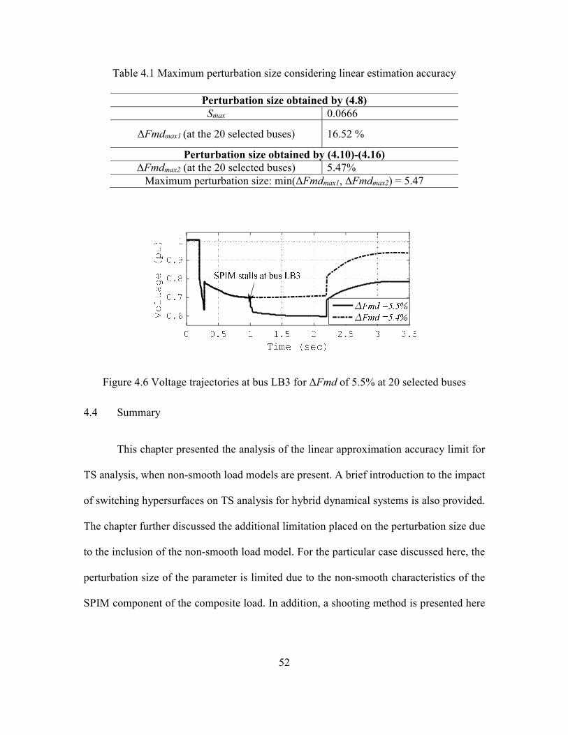
52
Table 4.1 Maximum perturbation size considering linear estimation accuracy
Perturbation size obtained by (4.8)
Smax 0.0666
ΔFmdmax1 (at the 20 selected buses) 16.52 %
Perturbation size obtained by (4.10)-(4.16)
ΔFmdmax2 (at the 20 selected buses) 5.47%
Maximum perturbation size: min(ΔFmdmax1, ΔFmdmax2) = 5.47
Figure 4.6 Voltage trajectories at bus LB3 for ΔFmd of 5.5% at 20 selected buses
4.4 Summary
This chapter presented the analysis of the linear approximation accuracy limit for
TS analysis, when non-smooth load models are present. A brief introduction to the impact
of switching hypersurfaces on TS analysis for hybrid dynamical systems is also provided.
The chapter further discussed the additional limitation placed on the perturbation size due
to the inclusion of the non-smooth load model. For the particular case discussed here, the
perturbation size of the parameter is limited due to the non-smooth characteristics of the
SPIM component of the composite load. In addition, a shooting method is presented here

53
to compute the maximum perturbation size, while taking into account the non-smooth be-
havior of the load model.

54
CHAPTER 5: COMMERCIAL IMPLEMENTATION OF TRAJECTORY SEN-
SITIVITY ANALYSIS
The previous chapters presented the application of TS analysis to quantify the im-
pact of load model parameter uncertainty on the power system algebraic and state variable
trajectories during dynamic simulations. The TS analysis module was implemented in
PSAT, which uses an implicit integration algorithm based TDS routine. It was shown in
Chapter 2 that using an analytical method for TS analysis in conjunction with an implicit
integration based TDS results in additional saving in computational time due to the struc-
ture of the problem. However, not all power system simulators are equipped with implicit
integration techniques. A majority of the commercially available power system simulators
like GE-PSLF and Siemens PSS/E use explicit integration based methods to perform the
dynamic simulations [22], [23]. As such, it is important to investigate the implementation
of the TS analysis module in commercial power system simulators, which use explicit in-
tegration routines. This chapter presents the implementation of a TS analysis in conjunction
with an explicit integration routine in PSAT. A comparison of the performance of TS with
explicit and implicit integration routine is also presented here. Furthermore, TS analysis is
implemented in GE-PSLF and the results are presented here.
5.1 Implicit versus explicit methods of numerical integration
A detailed discussion of implicit and explicit methods of integration can be found
in [36]. A brief discussion of the two methods in relation to solving differential algebraic
equations is presented in this section.

55
Consider a dynamic system described by
),,( λyxFx =& , and (5.1)
0),,( =λyxG . (5.2)
where, the description of the variables are the same as those given in (2.1) and (2.2). When
(5.1) and (5.2) are solved using an implicit method like the trapezoidal method [36], the
state variables x(t+Δt) and the algebraic variables y(t+ Δt) for the next time step are ob-
tained by solving
0))),(),(()),(),(((2
)()( =+∆+∆+∆−−∆+ λλ tytxFttyttxFt
txttx , and (5.3)
0)),(),(( =∆+∆+ λttyttxG . (5.4)
Since (5.3) and (5.4) are both nonlinear in x(t+Δt) and y(t+ Δt), (5.3) and (5.4) is
solved iteratively. When a Newton-Raphson method is employed to solve (5.3) and (5.4),
the Jacobian required at each step of the iteration is given by
∆∆−
yx
yx
GG
tF
tFI
22 . (5.5)
When (5.1) and (5.2) are solved using an explicit method of integration like a for-
ward Euler method [36], the state variables x(t+Δt) and the algebraic variables y(t+ Δt) for
the next time step is obtained by solving
))),(),((()()( λtytxFttxttx ∆+=∆+ , and (5.6)
56
0)),(),(( =∆+∆+ λttyttxG . (5.7)
In the explicit method, (5.6) is linear in x(t+Δt) and y(t+ Δt) and can be solved
directly to obtain x(t+Δt). However (5.7) is still nonlinear and has to be solved iteratively.
When a Newton-Raphson method is used to solve (5.6), the Jacobian at every step of the
iteration is given by Gy. In the context of power system TS analysis, Gy is the power flow
Jacobian. A comprehensive description of other explicit and implicit methods of integra-
tion can be found in [36].
Both the explicit and the implicit methods of integration have their advantages and
disadvantages. The implicit methods of integration are preferred when the underlying dy-
namic system has fast transient responses [36]. The method is more stable even with larger
simulation time steps Δt, as compared to an explicit method. Explicit methods of integra-
tion are recommended for systems with comparatively slower dynamics if a reasonably
large simulation time step Δt is to be used. The appropriate simulation time step Δt, is
dependent on the time constants of the dynamic system. Implicit methods of integration
require more computation for each time step of the simulation as compared to the explicit
methods. However, since a larger time step can be used for the implicit methods, the overall
computational burden can be significantly reduced when compared to explicit methods,
while integrating a fast dynamic system. Reference [36] provides a detailed discussion of
the time step selection, and the stability and accuracy of various explicit and implicit meth-
ods of integration. Electromagnetic transient programs (EMTP) which handle faster elec-

57
trical transients, use implicit methods of integration. The electromechanical transient sim-
ulators like PSLF and PSS/E which handle comparatively slower electromechanical tran-
sients, use explicit methods of integration.
5.2 Computing sensitivities using explicit integration
The sensitivity equations are repeated here for convenience. The sensitivity equa-
tions are given by
iFWFUF
dt
dU
d
dF
d
xdiyix
i
ii
λλλ++===
&, and (5.8)
iGWGUG
d
dGiyix
i
λλ++==0 . (5.9)
In Chapter 2, the sensitivity equations (2.5) and (2.6) were integrated using the
trapezoidal method. When an explicit method of integration like the forward Euler method
is used to compute the sensitivities, Ui(t+Δt) and Wi(t+Δt) are obtained by solving
)(2
)()(i
FWFUFt
tUttU iyixii λ++∆+=∆+ , and (5.10)
iGtWGttUG iyix λ−=∆++∆+ )()( . (5.11)
(5.9) and (5.10) can be re-written as a linear matrix equation given by

58
∆+−
++∆+
=
∆+∆+
∆+∆+
)(
)()()()()((2
)(
)(
)(
)()(
0
ttG
tFtWtFtUtFt
tU
ttW
ttU
ttGttG
I
i
iiyixi
i
i
yx
λ
λ
. (5.12)
For solving (5.12), the entries Fx (t), Fy (t), Fλi (t), Gx (t+Δt) and Gλi (t+Δt) need to
be evaluated additionally. The entry Gy(t+Δt) is obtained as a byproduct of solving (5.7)
during the TDS. Unlike the implicit integration based TS analysis, not all entries in the
coefficient matrix and the right hand side vector of (5.12) are available as a byproduct of
the TDS routine when an explicit integration algorithm is used. However, the additional
evaluation of those entries does not necessarily make the explicit integration based TS
analysis computationally more expensive. If an implicit integration method is used, the sub
matrices Fx, Fy, Gx and Gy, are computed at every iteration in each time step while solving
(5.3) and (5.4). The converged values of Fx, Fy, Gx and Gy are then used for evaluating the
trajectory sensitivities. In contrast, if an explicit integration method is used, the sub matri-
ces Fx, Fy and Gx are computed once every time step after the values of the algebraic and
state variables for that time is obtained. Therefore, the computational burden in an explicit
integration method would depend on the time step of simulation that can be permitted,
which is dependent on the underlying dynamic system.
5.2.1 Application of explicit integration based TS analysis in PSAT
The publicly available version of PSAT does not have an explicit integration rou-
tine. The explicit integration based TDS and the TS analysis routine was implemented in
PSAT based on (5.9)-(5.12). To compare the performance of the TS analysis using both
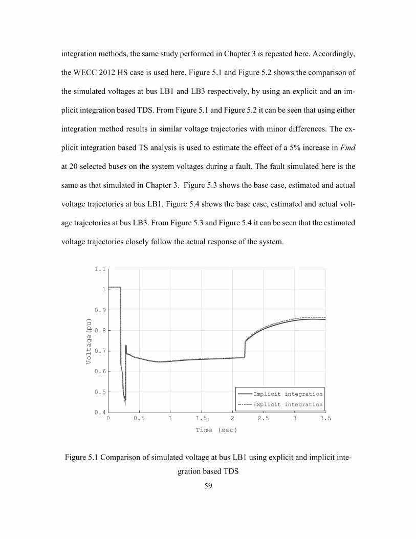
59
integration methods, the same study performed in Chapter 3 is repeated here. Accordingly,
the WECC 2012 HS case is used here. Figure 5.1 and Figure 5.2 shows the comparison of
the simulated voltages at bus LB1 and LB3 respectively, by using an explicit and an im-
plicit integration based TDS. From Figure 5.1 and Figure 5.2 it can be seen that using either
integration method results in similar voltage trajectories with minor differences. The ex-
plicit integration based TS analysis is used to estimate the effect of a 5% increase in Fmd
at 20 selected buses on the system voltages during a fault. The fault simulated here is the
same as that simulated in Chapter 3. Figure 5.3 shows the base case, estimated and actual
voltage trajectories at bus LB1. Figure 5.4 shows the base case, estimated and actual volt-
age trajectories at bus LB3. From Figure 5.3 and Figure 5.4 it can be seen that the estimated
voltage trajectories closely follow the actual response of the system.
Figure 5.1 Comparison of simulated voltage at bus LB1 using explicit and implicit inte-
gration based TDS
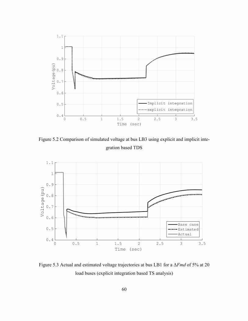
60
Figure 5.2 Comparison of simulated voltage at bus LB3 using explicit and implicit inte-
gration based TDS
Figure 5.3 Actual and estimated voltage trajectories at bus LB1 for a ΔFmd of 5% at 20
load buses (explicit integration based TS analysis)
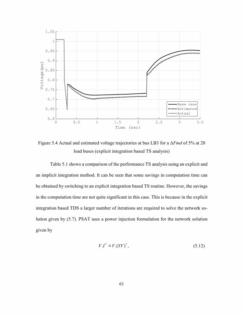
61
Figure 5.4 Actual and estimated voltage trajectories at bus LB3 for a ΔFmd of 5% at 20
load buses (explicit integration based TS analysis)
Table 5.1 shows a comparison of the performance TS analysis using an explicit and
an implicit integration method. It can be seen that some savings in computation time can
be obtained by switching to an explicit integration based TS routine. However, the savings
in the computation time are not quite significant in this case. This is because in the explicit
integration based TDS a larger number of iterations are required to solve the network so-
lution given by (5.7). PSAT uses a power injection formulation for the network solution
given by
** ).(. YVVIV = , (5.12)
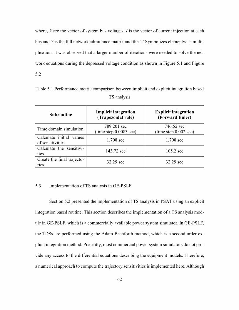
62
where, V are the vector of system bus voltages, I is the vector of current injection at each
bus and Y is the full network admittance matrix and the ‘.’ Symbolizes elementwise multi-
plication. It was observed that a larger number of iterations were needed to solve the net-
work equations during the depressed voltage condition as shown in Figure 5.1 and Figure
5.2
Table 5.1 Performance metric comparison between implicit and explicit integration based
TS analysis
Subroutine Implicit integration
(Trapezoidal rule)
Explicit integration
(Forward Euler)
Time domain simulation 789.201 sec
(time step 0.0083 sec)
746.52 sec
(time step 0.002 sec)
Calculate initial values
of sensitivities 1.708 sec 1.708 sec
Calculate the sensitivi-
ties 143.72 sec 105.2 sec
Create the final trajecto-
ries 32.29 sec 32.29 sec
5.3 Implementation of TS analysis in GE-PSLF
Section 5.2 presented the implementation of TS analysis in PSAT using an explicit
integration based routine. This section describes the implementation of a TS analysis mod-
ule in GE-PSLF, which is a commercially available power system simulator. In GE-PSLF,
the TDSs are performed using the Adam-Bashforth method, which is a second order ex-
plicit integration method. Presently, most commercial power system simulators do not pro-
vide any access to the differential equations describing the equipment models. Therefore,
a numerical approach to compute the trajectory sensitivities is implemented here. Although
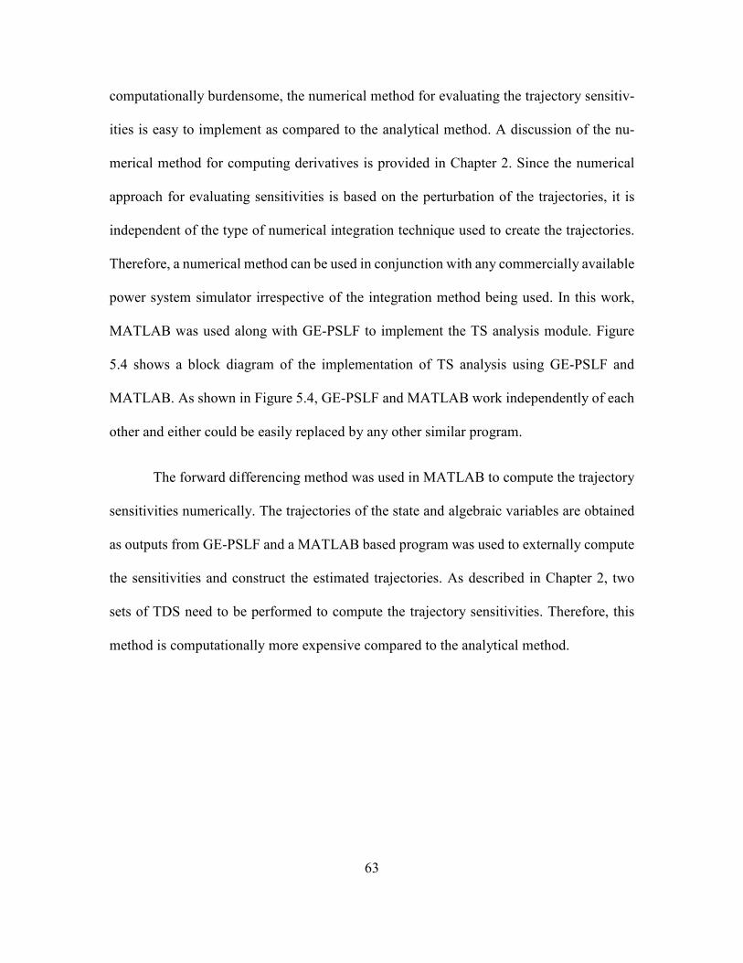
63
computationally burdensome, the numerical method for evaluating the trajectory sensitiv-
ities is easy to implement as compared to the analytical method. A discussion of the nu-
merical method for computing derivatives is provided in Chapter 2. Since the numerical
approach for evaluating sensitivities is based on the perturbation of the trajectories, it is
independent of the type of numerical integration technique used to create the trajectories.
Therefore, a numerical method can be used in conjunction with any commercially available
power system simulator irrespective of the integration method being used. In this work,
MATLAB was used along with GE-PSLF to implement the TS analysis module. Figure
5.4 shows a block diagram of the implementation of TS analysis using GE-PSLF and
MATLAB. As shown in Figure 5.4, GE-PSLF and MATLAB work independently of each
other and either could be easily replaced by any other similar program.
The forward differencing method was used in MATLAB to compute the trajectory
sensitivities numerically. The trajectories of the state and algebraic variables are obtained
as outputs from GE-PSLF and a MATLAB based program was used to externally compute
the sensitivities and construct the estimated trajectories. As described in Chapter 2, two
sets of TDS need to be performed to compute the trajectory sensitivities. Therefore, this
method is computationally more expensive compared to the analytical method.
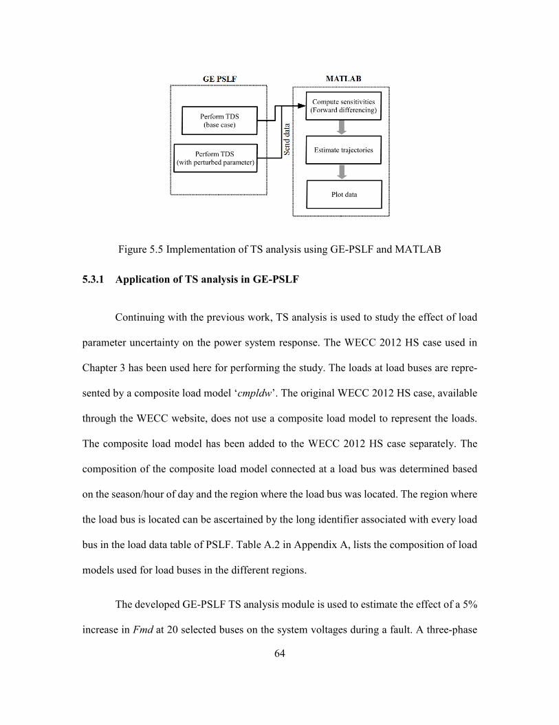
64
Figure 5.5 Implementation of TS analysis using GE-PSLF and MATLAB
5.3.1 Application of TS analysis in GE-PSLF
Continuing with the previous work, TS analysis is used to study the effect of load
parameter uncertainty on the power system response. The WECC 2012 HS case used in
Chapter 3 has been used here for performing the study. The loads at load buses are repre-
sented by a composite load model ‘cmpldw’. The original WECC 2012 HS case, available
through the WECC website, does not use a composite load model to represent the loads.
The composite load model has been added to the WECC 2012 HS case separately. The
composition of the composite load model connected at a load bus was determined based
on the season/hour of day and the region where the load bus was located. The region where
the load bus is located can be ascertained by the long identifier associated with every load
bus in the load data table of PSLF. Table A.2 in Appendix A, lists the composition of load
models used for load buses in the different regions.
The developed GE-PSLF TS analysis module is used to estimate the effect of a 5%
increase in Fmd at 20 selected buses on the system voltages during a fault. A three-phase
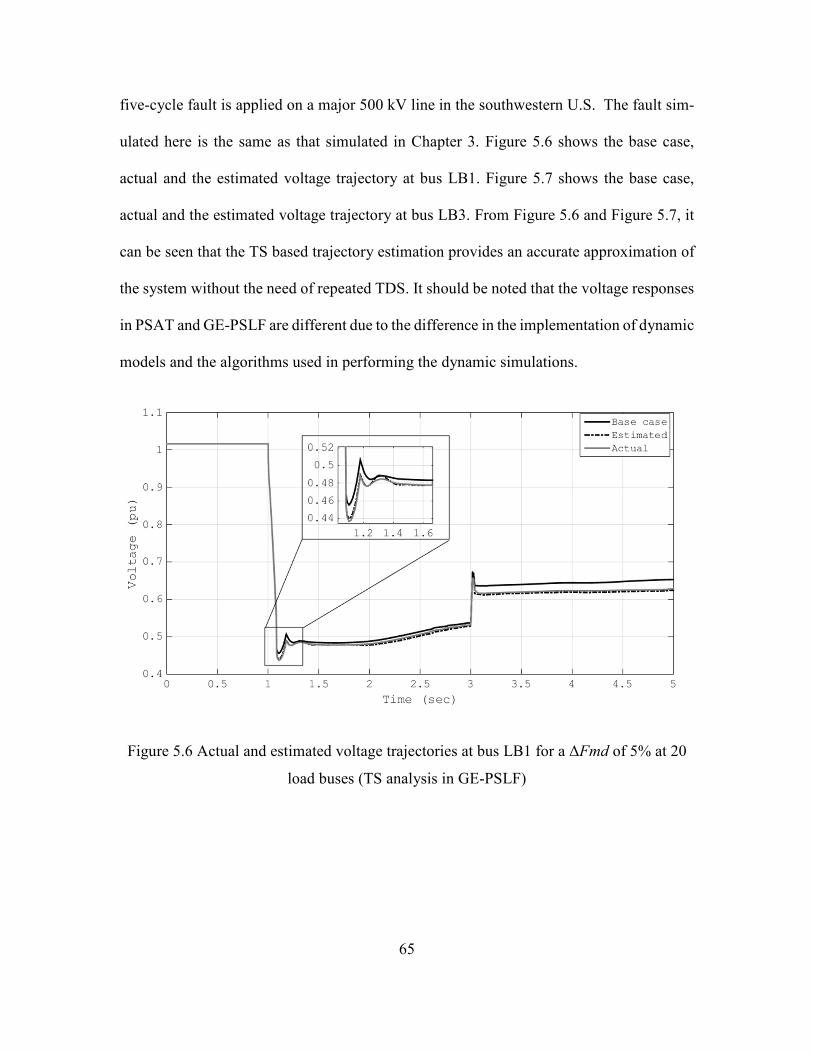
65
five-cycle fault is applied on a major 500 kV line in the southwestern U.S. The fault sim-
ulated here is the same as that simulated in Chapter 3. Figure 5.6 shows the base case,
actual and the estimated voltage trajectory at bus LB1. Figure 5.7 shows the base case,
actual and the estimated voltage trajectory at bus LB3. From Figure 5.6 and Figure 5.7, it
can be seen that the TS based trajectory estimation provides an accurate approximation of
the system without the need of repeated TDS. It should be noted that the voltage responses
in PSAT and GE-PSLF are different due to the difference in the implementation of dynamic
models and the algorithms used in performing the dynamic simulations.
Figure 5.6 Actual and estimated voltage trajectories at bus LB1 for a ΔFmd of 5% at 20
load buses (TS analysis in GE-PSLF)
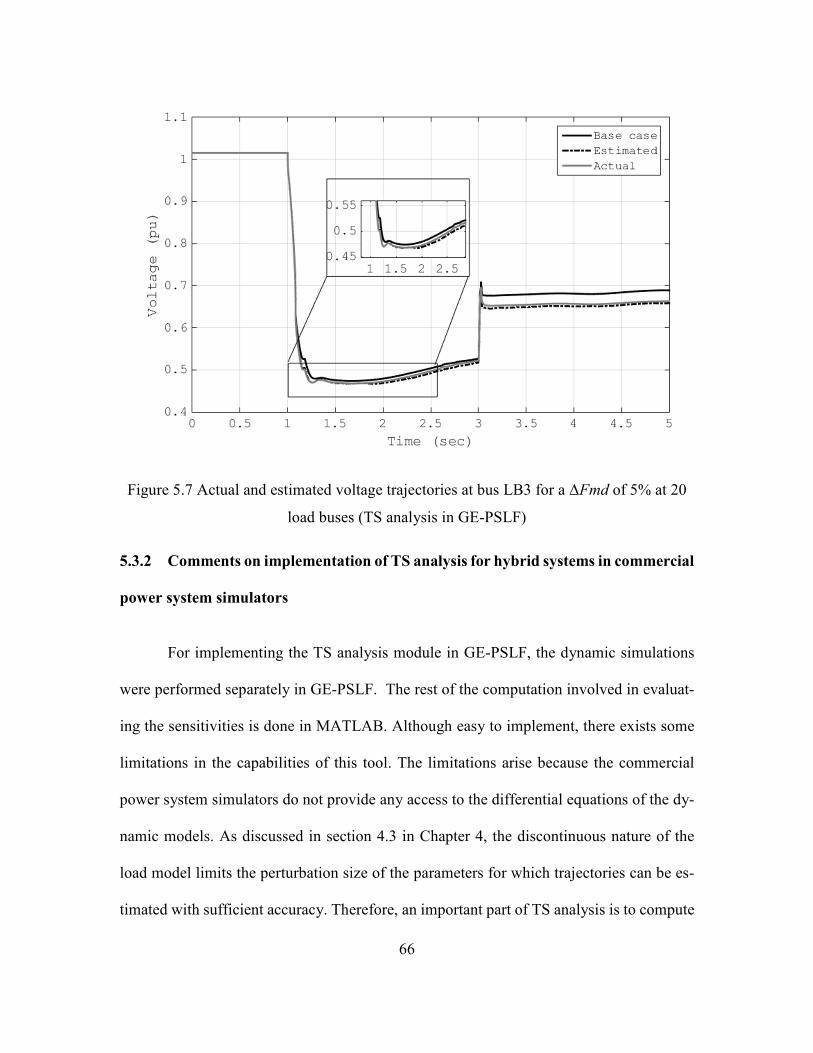
66
Figure 5.7 Actual and estimated voltage trajectories at bus LB3 for a ΔFmd of 5% at 20
load buses (TS analysis in GE-PSLF)
5.3.2 Comments on implementation of TS analysis for hybrid systems in commercial
power system simulators
For implementing the TS analysis module in GE-PSLF, the dynamic simulations
were performed separately in GE-PSLF. The rest of the computation involved in evaluat-
ing the sensitivities is done in MATLAB. Although easy to implement, there exists some
limitations in the capabilities of this tool. The limitations arise because the commercial
power system simulators do not provide any access to the differential equations of the dy-
namic models. As discussed in section 4.3 in Chapter 4, the discontinuous nature of the
load model limits the perturbation size of the parameters for which trajectories can be es-
timated with sufficient accuracy. Therefore, an important part of TS analysis is to compute
67
the limit on the perturbation size for which trajectory estimation is valid. However, in the
numerical approach to TS analysis, substantial additional computation is required for eval-
uating the maximum perturbation size by the shooting method as given by (4.10) – (4.20).
Due to the inability to access to the model differential equations, all entries of the Jacobian
given by (4.21) have to be computed numerically by a finite differencing method. This
requires multiple perturbed TDSs, thereby substantially increasing the computational bur-
den. It is therefore important to implement the TS analysis using the analytical method in
commercial power system simulators. This can be done in the same way as TS analysis
was implemented in PSAT using an explicit integration in section 5.2. It should however
be pointed out that PSAT uses a power injection model for representing the network equa-
tions given by (5.12). In contrast, most commercial power system simulators use a current
injection model for the representing the network equations in the TDS modules. In the
current injection model, only the active nodes in the network are retained for solving net-
work equations. The generators and nonlinear loads with voltage dependent current injec-
tions are represented by their Norton’s equivalent. The network equations using the current
injection model is given by
VYredI )(= (5.13)
where, Yred is the reduced Y matrix of (5.12), which retains only the active nodes of the
system. This formulation is particularly favored because the size of the matrix Yred is less
than the complete admittance matrix Y. Additionally, (5.13) is typically solved using
Gauss-Jacobi iterations instead of the Newton-Raphson method, as used in PSAT. While
68
implementing the TS analysis module in this framework, unlike PSAT, the entry Gy is not
available and needs to be evaluated separately.
5.4 Summary
This chapter describes the implementation of TS analysis using an explicit integra-
tion based TDS. A comparison of the explicit integration based TS analysis with an implicit
integration based TS analysis is presented here. Furthermore, the implementation of TS
analysis in GE-PSLF a commercially available power system simulator using the present
infrastructure is presented here. This chapter also presents an additional discussion on the
limitation of the current implementation of TS analysis in the existing commercial power
system simulators. It highlights the need to move to an analytical approach for TS analysis
rather than pursuing a numerical approach.

69
CHAPTER 6: SENSITIVITY BASED PARAMETER ESTIMATION
Simulation studies play a crucial role in power system operations and planning.
Simulation studies enable system operators and planners to study the behavior of key trans-
mission and generation components under different operating conditions, and to ensure the
security and reliability of the system. These studies rely heavily on the accuracy of the
mathematical models used to represent the various transmission and generation equipment.
The simulation models are expected to replicate the behavior of the actual component in a
reasonably accurate manner. Therefore, estimating the model parameters precisely is of
paramount importance. Parameter estimation techniques for generators and other major
transmission and distribution components are well-established [49-52]. The model param-
eters are typically estimated based on field-testing of these components as well as from
manufacturers’ data [49-52]. In recent years, parameter estimation in load modeling has
gained considerable importance [15], [53], [54]. This is due to the increasing focus on the
development of accurate load models for power system studies. Since the consumer loads
(both commercial and residential) are represented as aggregated loads at the distribution
substation, determination of parameters for the aggregated load model is challenging [15],
[53], and [54]. Presently, the utilities determine such load models based on the measure-
ments made at substations and by testing the performance of common consumer loads like
induction motors and electronic loads [15]. However, aggregated load models have a large
number of tunable parameters, which makes the task of parameter estimation challenging.
This chapter describes a tool that can be used to estimate model parameter, which focuses
on aggregated load model parameter estimation. The tool presented here uses a sensitivity-
based approach to estimate multiple model parameters based on recorded measurements of

70
voltage, active and reactive power at the substation bus of interest. A nonlinear least
squares minimization method is used to estimate the parameters. The output of the model
(active and reactive power) based on the terminal voltage and an initial guess of the param-
eters is compared to the actual measurements. The parameters are then adjusted iteratively
to reduce the error between the model output and the actual measured output. The proposed
tool provides a convenient method to estimate the model parameters such that the simula-
tion results can replicate the actual system response.
Apart from tuning model parameters based on measurements, the tool can be useful
in tuning parameters such that comparable results can be obtained between different simu-
lation tools. This can be done by using the simulation output of a reliable tool and then
using this output as measurements to tune the model parameters in a different tool. This is
particularly significant as the power system simulation industry is seeing a surge in open
source simulation tools. One of the main issues with open source tools is replicating the
results of simulations with the established commercial power system simulators. One of
the main reasons for the observed discrepancies is the difference in the mathematical im-
plementation of the various equipment models across different simulation tools. Tuning
the model parameters, such that open source tools can replicate the simulation outputs
could be a significant step towards the advancement of such open source tools. However,
this is envisaged as a secondary use of the tool and the primary use remains for parameter
estimation based on actual field measurements.
The following sections present brief discussions on the nonlinear least squares min-
imization and the sensitivity based parameter estimation process. A numerical example

71
showing the application of the tool to estimate the composite load model parameters is also
presented here.
6.1 Nonlinear least squares minimization
The nonlinear least squares minimization technique is a common method used for
curve fitting. The curve-fitting problem can be framed as least square minimization prob-
lem given by [55]
[ ] [ ])()()(minarg λλλλ
FmFmet −−= , (6.1)
where,
m is the vector of data points corresponding to the measured data,
F(λ) is the vector of values of the curve to be fitted, evaluated for a particular value of λ,
e(λ) is the λ dependent square of the error, which is the objective function being minimized,
and
λ is the vector of variables that are updated to minimize e(λ)
The trust region methods are established algorithms to solve the nonlinear least
squares problem given by (1) [55]. Detailed descriptions of these methods can be found in
[55]. The Gauss-Newton [55] and Levenberg-Marquardt [55] are the most popular and ef-
fective trust region methods used for solving the nonlinear least squares problem. In the
Gauss-Newton method, the parameter set λ is updated by an amount Δλ at each iteration of
the optimization process, where Δλ is given by [55]

72
))(()( 1 λλ FmJJJ tt −=∆ − , (6.2)
λλ
∂∂= )(F
J , (6.3)
where, J is the Jacobian with respect to the parameter set λ. The main drawback of the
Gauss-Newton method is that it requires the matrix JtJ to be invertible.
The Levenberg-Marquardt method works better than the Gauss-Newton method
when the matrix JtJ is ill conditioned or singular. In the Levenberg-Marquardt method, the
parameter set λ is updated by [55]
))(())diag( ( 1 λµλ FmJJJJJ ttt −+=∆ − , (6.4)
where, µ is a damping factor that is computed adaptively at each step of the iteration based
on the computed error between m and F(λ). The additional term µdiag(JtJ) prevents the
inverted part of (6.4) to be singular [55], [56]. The Jacobian matrix given by (6.3) can be
computed either numerically using a finite differencing approach or analytically.
6.2 Effect of parameter sensitivity on the estimation process
The Jacobian matrix provides useful information about the parameter estimation
process. For the load model parameter estimation problem, the elements of the Jacobian
matrix are the sensitivities of the consumed active and reactive power to the parameters to
be estimated. Since the number of data points obtained by measurements is typically more
than the number of parameters to be estimated, the Jacobian matrix has more rows than
columns. For the parameter estimation to be accurate, the Jacobian given by (6.3) should

73
have full column rank. For a column rank deficient Jacobian matrix, not all parameters in
the parameter set can be identified uniquely. The Jacobian can be rank deficient or close
to rank deficiency for two reasons:
1. A particular parameter being estimated may have little or no impact on the
measurements used. Therefore, the sensitivity of the particular measure-
ment/model output to the parameter is zero or nearly zero, thereby making the
Jacobian rank deficient.
2. A set of parameters may have identical impact on the measurement/model out-
put and hence two or more columns of the Jacobian matrix may be linearly
dependent. The linear dependence of the columns makes the Jacobian matrix
rank deficient in this case.
In both the conditions described here, certain parameters of the load model cannot
be estimated uniquely. When the Jacobian is column rank deficient or close to being col-
umn rank deficient the term,
)diag( JJJJ tt µ+ , (6.5)
may be ill conditioned. A detailed discussion on solving nonlinear least squares problem
with a rank deficient Jacobian can be found in [56].
In the context of model parameter estimation, analyzing the Jacobian J reveals if
the measurements made are sufficient for estimating a desired set of parameters. For a
given mathematical model of the load, the measurements recorded for parameter estimation

74
should clearly reflect the influence of the individual parameters, such that they can be es-
timated uniquely. When columns of the Jacobian matrix J are zero, the parameters associ-
ated with those particular columns will retain the initial guess values at the end of the esti-
mation process. These parameters do not have any influence on the dynamic behavior of
the model for a particular event, for which, the measurements have been made. If two or
more columns are linearly dependent on each other, the parameters associated with those
columns may or may not have significant effect on the model behavior. However, even if
the effect is significant the parameters cannot be identified uniquely because small changes
in the parameters have a similar impact on the dynamic behavior of the model for the par-
ticular event.
For the estimation error to be minimum, the Jacobian J should have full rank and
the matrix JtJ should not be ill-conditioned. When these conditions are satisfied, the pa-
rameters can be estimated uniquely with minimum error. As a practice both these indices,
rank of Jacobian J and the condition number JtJ, should be investigated prior to proceeding
with the parameter estimation process. JtJ is the approximate Hessian matrix in the least
square minimization process. This matrix provides information about the curvature of the
problem at any step of the iteration; that is, the rate of change of the sensitivities.
6.3 The composite load model parameter estimation
An example of load model parameter estimation is presented here. The parameters
of the composite load model developed in PSAT [40], a MATLAB based open source
power system simulator, is estimated here. This model is similar to the WECC composite

75
load model ‘cmpldw’ in GE-PSLF [22]. The example presented here serves to test the pro-
posed tool rather than present an actual case of measurement based parameter estimation.
In the absence of actual field measurements, the composite load model parameters are es-
timated based on surrogate voltage and, active and reactive power recorded from a detailed
three phase electromagnetic transient simulator. To obtain the measurements, a detailed
model of the composite load was used in PSCAD/EMTDC [57]. Furthermore, the entire
system in PSCAD/EMTDC is simulated in its full three phase details using a point on wave
simulation. As such, the measurements made in PSCAD/EMTDC serve as an efficient sur-
rogate for actual field measurements. The parameter estimation problem presented here,
serves as a good example to test the efficiency of the proposed tool. In PSCAD, the single-
phase induction motor (SPIM) driven air-conditioners (A/C) and the three phase induction
motors are represented by detailed differential equations describing the behavior of the
internal flux linkages in full three-phase details. However, the composite load model in
PSAT is represented by positive sequence models of three-phase induction motors and a
performance model of a SPIM driven A/C. The performance model of the SPIM driven
A/C is described by algebraic equations governing the active and reactive power consump-
tion depending on the terminal voltage. A detailed description of the SPIM driven A/C
model in PSCAD can be found in [58].The detailed description of the SPIM driven A/C in
PSAT can be found in [41]. The example highlights the efficiency of estimating the param-
eters of an approximate positive sequence load model from a detailed three-phase model
load model.
The IEEE 9 bus system was used in PSCAD to simulate a disturbance scenario and
record the voltage, active and reactive power at the load bus. Figure 6.1 shows the one line

76
diagram of the IEEE 9 bus system designed in PSCAD. Figure 6.2 shows the details of the
composite load model connected at bus 5 in PSCAD. The total load at bus 5 in Figure 6.2
is equally divided on the three 12.47 kV distribution feeders. Table 6.1 lists the composi-
tion of the load connected on each 12.47 kV feeder. As discussed in the previous section,
the disturbance should be chosen such that all the parameters to be estimated are expected
to have some impact on the dynamic behavior. For example, if the parameters affecting the
stalled behavior of an induction motor is to be estimated, the recorded measurements
should correspond to an event where the induction motor stalls. To achieve this, a three-
phase fault for 0.05 s was applied on bus 5. The fault creates a voltage dip sufficiently long
for the SPIM driven A/C to stall thereby resulting in a delayed voltage recovery. Figure 6.3
shows the voltage recorded at the low voltage side of the transformer connected at bus 5 in
PSCAD. Figure 6.4 and Figure 6.5 show the active and reactive power consumed by the
load connected at bus 5 respectively. These recorded measurements serve as inputs to the
parameter estimation tool presented here. Figure 6.6 shows the individual components of
composite load model in PSAT. The parameters of this model are estimated using the
measurements made from the detailed three-phase model in PSCAD. To estimate the load
parameters:
1. The voltage recorded in PSCAD is played in at the terminal bus of the load model
in the estimation tool as shown in Figure 6.6,
2. The active and reactive power consumed by the load model based on the initial
guess of the parameters is computed; and

77
3. The parameter values are then updated such that the least square error between the
computed active and reactive power and the recorded active and reactive power in
PSCAD is minimized.
Table 6.1 Component wise consumption of the composite load model
Load component Steady state load (MW/MVAr)
1-Ф A/C motor 24.3 + j6.5 MVA
3-Ф, constant torque motor (A) (torque proportional
to square of speed)
2.5 + j1.2 MVA
3-Ф, variable torque and low inertia motor (B)
(torque proportional to square of speed)
4.1 + j2.1 MVA
Static load 8.1 + j6.8 MVA
Total load 40+j16.6 MVA
Figure 6.1 One-line diagram of the IEEE 9 bus system
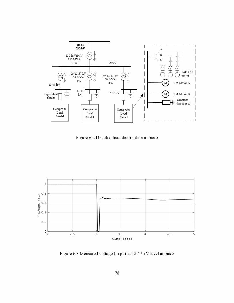
78
Figure 6.2 Detailed load distribution at bus 5
Figure 6.3 Measured voltage (in pu) at 12.47 kV level at bus 5
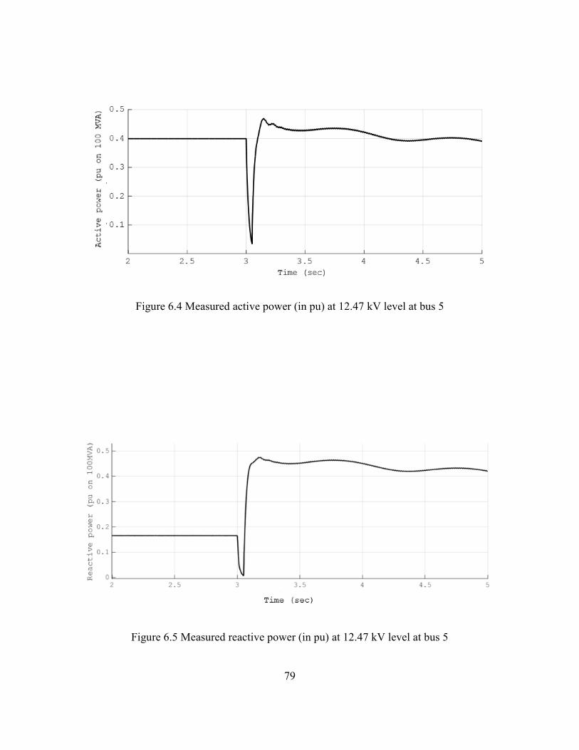
79
Figure 6.4 Measured active power (in pu) at 12.47 kV level at bus 5
Figure 6.5 Measured reactive power (in pu) at 12.47 kV level at bus 5
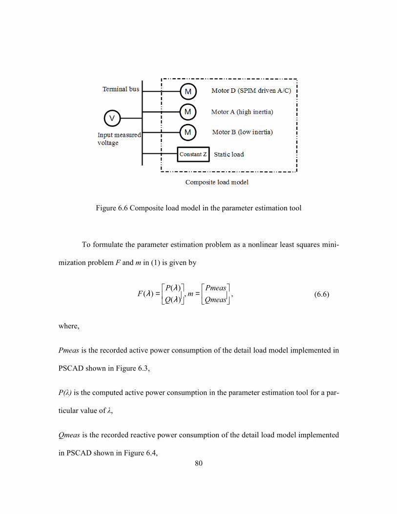
80
Figure 6.6 Composite load model in the parameter estimation tool
To formulate the parameter estimation problem as a nonlinear least squares mini-
mization problem F and m in (1) is given by
=
=
Qmeas
Pmeasm
Q
PF ,
)(
)()(
λλ
λ , (6.6)
where,
Pmeas is the recorded active power consumption of the detail load model implemented in
PSCAD shown in Figure 6.3,
P(λ) is the computed active power consumption in the parameter estimation tool for a par-
ticular value of λ,
Qmeas is the recorded reactive power consumption of the detail load model implemented
in PSCAD shown in Figure 6.4,

81
Q(λ) is the computed reactive power consumption in the parameter estimation tool for a
particular value of λ,
λ is a vector of parameters to be estimated, and the Jacobian J in (3) for the load model
parameter estimation is given by
tQP
J
∂∂
∂∂=
λλ
λλ )()(
. (6.7)
J is computed analytically for this work as it saves the additional computations required in
the finite differencing approach. However, a provision to compute the Jacobian by finite
differencing is included in the tool, which is useful when it is cumbersome to compute
certain entries of the J analytically.
Table 6.2 lists the parameters of the composite load model that are estimated in this
example. As shown in Table 6.2, 27 parameters are estimated in this example. The 27 se-
lected parameters are the key parameters in the composite load model. The parameters
relating to contactor trip or relay tripping are excluded here as these parameters introduce
discontinuities in the minimization problem.
Table 6.3 lists the initial guess used for the parameters in the estimation process.
Table 6.4 lists the upper and the lower bound on the parameter values. It is important to set
the upper and lower bounds properly based on some survey or prior experience. In the
absence of upper and lower bounds, the minimization routine can return unrealistic values
for the various parameters being estimated. The Levenberg-Marquardt method in the least
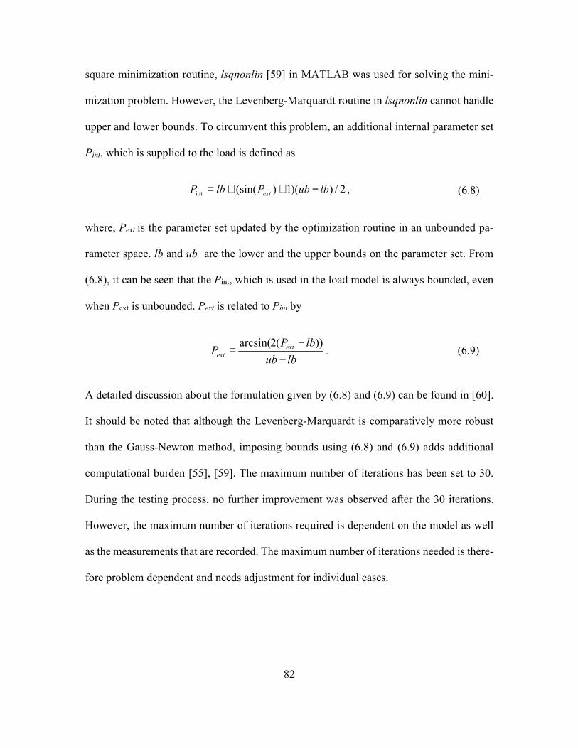
82
square minimization routine, lsqnonlin [59] in MATLAB was used for solving the mini-
mization problem. However, the Levenberg-Marquardt routine in lsqnonlin cannot handle
upper and lower bounds. To circumvent this problem, an additional internal parameter set
Pint, which is supplied to the load is defined as
2/))(1)(sin(int lbubPlbP ext −++= , (6.8)
where, Pext is the parameter set updated by the optimization routine in an unbounded pa-
rameter space. lb and ub are the lower and the upper bounds on the parameter set. From
(6.8), it can be seen that the Pint, which is used in the load model is always bounded, even
when Pext is unbounded. Pext is related to Pint by
lbub
lbPP ext
ext −−
=))(2arcsin(
. (6.9)
A detailed discussion about the formulation given by (6.8) and (6.9) can be found in [60].
It should be noted that although the Levenberg-Marquardt is comparatively more robust
than the Gauss-Newton method, imposing bounds using (6.8) and (6.9) adds additional
computational burden [55], [59]. The maximum number of iterations has been set to 30.
During the testing process, no further improvement was observed after the 30 iterations.
However, the maximum number of iterations required is dependent on the model as well
as the measurements that are recorded. The maximum number of iterations needed is there-
fore problem dependent and needs adjustment for individual cases.
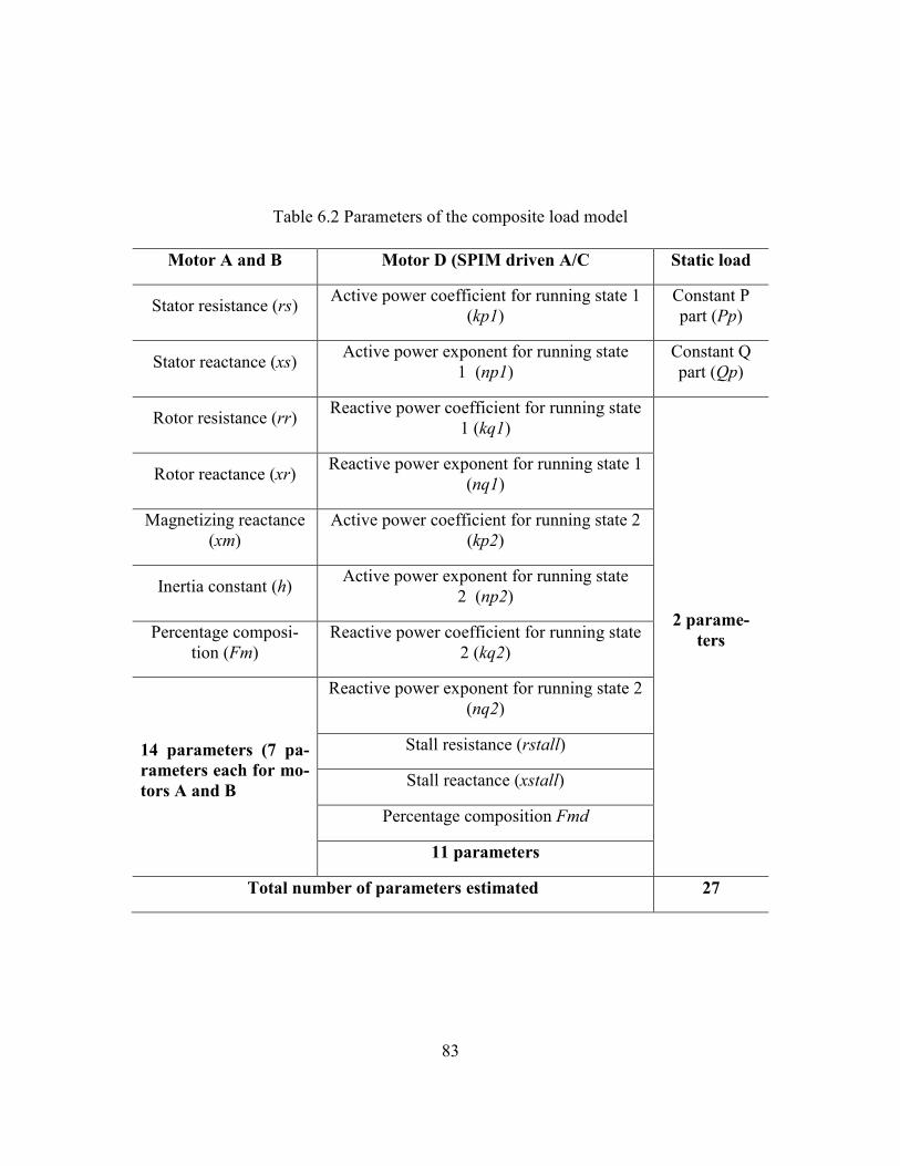
83
Table 6.2 Parameters of the composite load model
Motor A and B Motor D (SPIM driven A/C Static load
Stator resistance (rs) Active power coefficient for running state 1
(kp1)
Constant P
part (Pp)
Stator reactance (xs) Active power exponent for running state
1 (np1)
Constant Q
part (Qp)
Rotor resistance (rr) Reactive power coefficient for running state
1 (kq1)
2 parame-
ters
Rotor reactance (xr) Reactive power exponent for running state 1
(nq1)
Magnetizing reactance
(xm)
Active power coefficient for running state 2
(kp2)
Inertia constant (h) Active power exponent for running state
2 (np2)
Percentage composi-
tion (Fm)
Reactive power coefficient for running state
2 (kq2)
14 parameters (7 pa-
rameters each for mo-
tors A and B
Reactive power exponent for running state 2
(nq2)
Stall resistance (rstall)
Stall reactance (xstall)
Percentage composition Fmd
11 parameters
Total number of parameters estimated 27
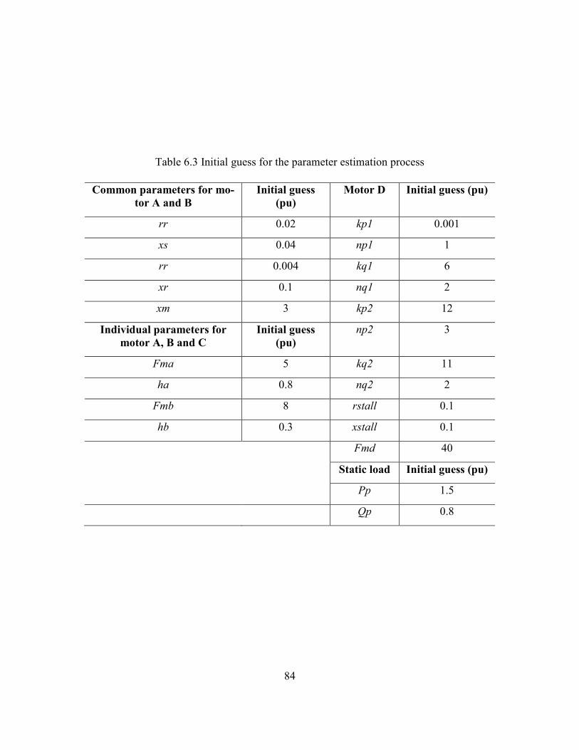
84
Table 6.3 Initial guess for the parameter estimation process
Common parameters for mo-
tor A and B
Initial guess
(pu)
Motor D Initial guess (pu)
rr 0.02 kp1 0.001
xs 0.04 np1 1
rr 0.004 kq1 6
xr 0.1 nq1 2
xm 3 kp2 12
Individual parameters for
motor A, B and C
Initial guess
(pu)
np2 3
Fma 5 kq2 11
ha 0.8 nq2 2
Fmb 8 rstall 0.1
hb 0.3 xstall 0.1
Fmd 40
Static load Initial guess (pu)
Pp 1.5
Qp 0.8
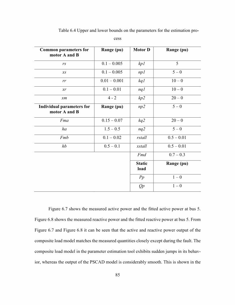
85
Table 6.4 Upper and lower bounds on the parameters for the estimation pro-
cess
Common parameters for
motor A and B
Range (pu) Motor D Range (pu)
rs 0.1 – 0.005 kp1 5
xs 0.1 – 0.005 np1 5 – 0
rr 0.01 – 0.001 kq1 10 – 0
xr 0.1 – 0.01 nq1 10 – 0
xm 4 - 2 kp2 20 – 0
Individual parameters for
motor A and B
Range (pu) np2 5 – 0
Fma 0.15 – 0.07 kq2 20 – 0
ha 1.5 – 0.5 nq2 5 – 0
Fmb 0.1 – 0.02 rstall 0.5 – 0.01
hb 0.5 – 0.1 xstall 0.5 – 0.01
Fmd 0.7 – 0.3
Static
load
Range (pu)
Pp 1 – 0
Qp 1 – 0
Figure 6.7 shows the measured active power and the fitted active power at bus 5.
Figure 6.8 shows the measured reactive power and the fitted reactive power at bus 5. From
Figure 6.7 and Figure 6.8 it can be seen that the active and reactive power output of the
composite load model matches the measured quantities closely except during the fault. The
composite load model in the parameter estimation tool exhibits sudden jumps in its behav-
ior, whereas the output of the PSCAD model is considerably smooth. This is shown in the

86
insets of Figure 6.7 and Figure 6.8. The discrepancy can be attributed to the modeling
differences in the SPIM driven A/C model in PSCAD and PSAT. As mentioned before, in
PSCAD the flux decay in the SPIM and the rotation of its shaft is described by differential
equations. However, in PSAT, the SPIM is represented by a performance model, which is
purely algebraic and has discontinuities. The sharp jumps in the output of the tuned PSAT
model are due to the transition of the SPIM from one operating state to another. However,
before the fault and approximately 0.4 s after the fault is removed, the output of PSAT
model with the estimated parameters closely matches with the PSCAD model. The esti-
mated values of the parameters are listed in Table 6.4. The estimation process was repeated
using the Gauss-Newton algorithm in lsqnonlin. The Gauss-Newton algorithm supports the
upper and lower bounds on the parameters values. The estimated values of the parameter
are listed in Table 6.6.
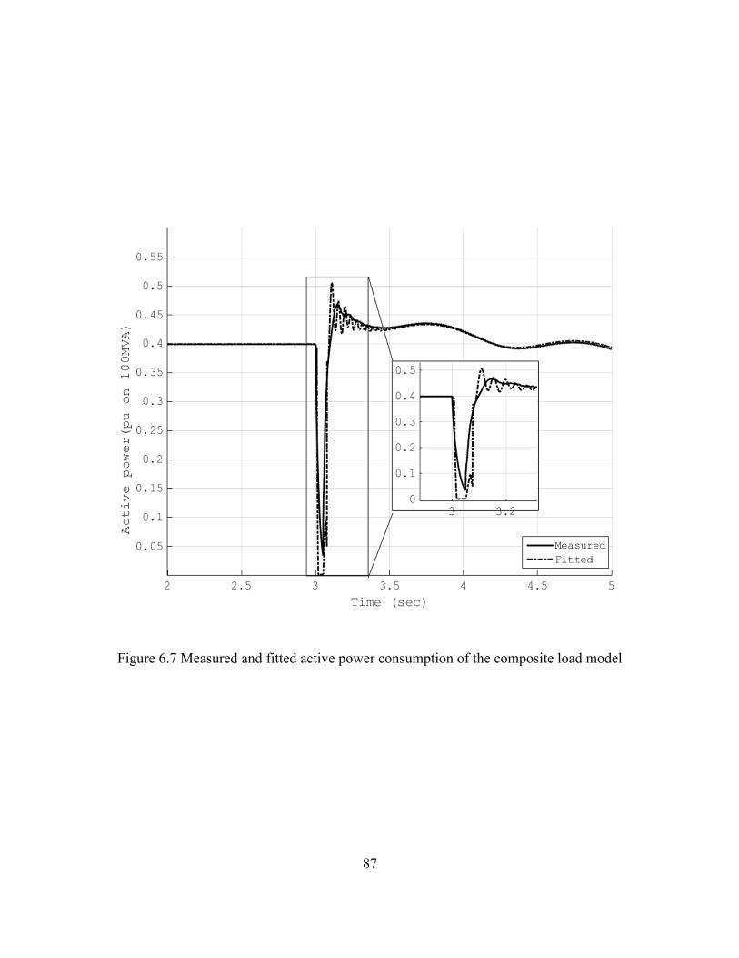
87
Figure 6.7 Measured and fitted active power consumption of the composite load model

88
Figure 6.8 Measured and fitted reactive power consumption of the composite load model
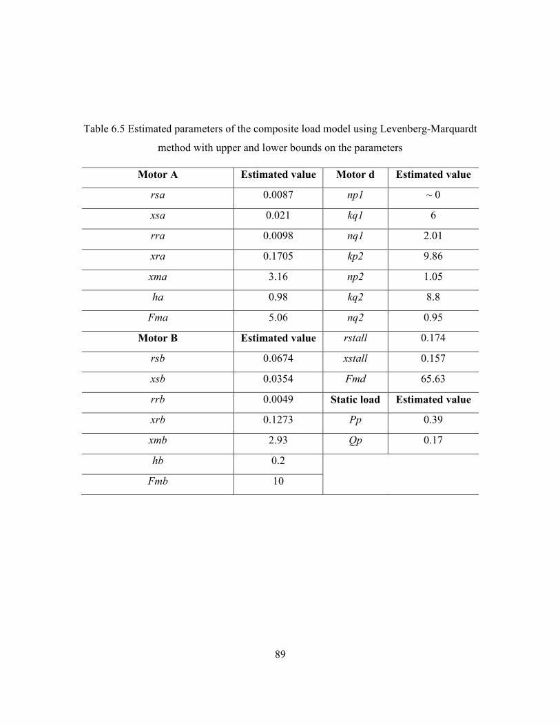
89
Table 6.5 Estimated parameters of the composite load model using Levenberg-Marquardt
method with upper and lower bounds on the parameters
Motor A Estimated value Motor d Estimated value
rsa 0.0087 np1 ~ 0
xsa 0.021 kq1 6
rra 0.0098 nq1 2.01
xra 0.1705 kp2 9.86
xma 3.16 np2 1.05
ha 0.98 kq2 8.8
Fma 5.06 nq2 0.95
Motor B Estimated value rstall 0.174
rsb 0.0674 xstall 0.157
xsb 0.0354 Fmd 65.63
rrb 0.0049 Static load Estimated value
xrb 0.1273 Pp 0.39
xmb 2.93 Qp 0.17
hb 0.2
Fmb 10

90
Table 6.6 Estimated parameters of the composite load model using Gauss-Newton
method with upper and lower bounds on the parameters
Motor A Estimated value Motor d Estimated value
rsa 0.0083 np1 ~ 0
xsa 0.041 kq1 6
rra 0.0078 nq1 2.03
xra 0.153 kp2 9.72
xma 2.99 np2 1.05
ha 0.88 kq2 8.802
Fma 6.26 nq2 0.95
Motor B Estimated value rstall 0.1735
rsb 0.0611 xstall 0.16
xsb 0.0375 Fmd 64.51
rrb 0.0040 Static load Estimated value
xrb 0.137 Pp 0.39
xmb 3.01 Qp 0.17
hb 0.202
Fmb 10

91
6.3.1 Load model parameter sensitivity and dependency
The entries of the matrix J are the sensitivities of the active and reactive power
consumed by the load to the load model parameters being estimated. As discussed before,
a low column rank of J may introduce error in the parameter estimation process. In this
particular case of load model parameter estimation, a low column rank of J indicates that
1. the recorded measurements of active and reactive power may not be sensi-
tive to the load parameters of interest, or
2. two or more parameters may have similar sensitivities for the recorded
measurements.
Analyzing and understanding the implications of these two different conditions,
provides additional insight into the parameter estimation process. References [53] and [54],
uses the Jacobian to reduce the parameter space by removing the less sensitive parameters.
However, a systematic method is not introduced in [53] or [54]. To analyze the Jacobian
J; the pairwise condition number for each column of J with all other columns is computed.
A large condition number indicates either that the entries of one column is nearly zero or
that the two columns are linearly dependent. Figure 6.9 and Figure 6.10 shows the pairwise
condition numbers of the important parameters of the composite load model for the active
and reactive power measurements respectively. The parameters kp1, np1, kp2, np2, kq1,
nq1, kq2, and nq2 are left out of Figure 6.9 and Figure 6.10 because these parameters did
not significantly affect the model. The condition numbers were computed for the Jacobian
J at the beginning of the iteration with the initial guesses for the parameters.

92
The relatively large pairwise condition numbers are highlighted in both Figure 6.9
and Figure 6.10. The key observations from Figure 6.9 and Figure 6.10 are as follows:
1. In Figure 9, the pairwise condition numbers for the parameter Qp are very
high. This is because the column entries of J corresponding to the parameter
Qp is zero for the active power measurements. Qp has no impact on the
active power consumption of the composite load model. Changes in the pa-
rameter Qp only impacts the reactive power consumption of the model. Fig-
ure 11 and Figure 12 show the sensitivity of the active and reactive power
consumed by the load to the parameters Pp and Qp. From Figure 11 and
Figure 12 it can be seen that both the active and reactive power consumption
is sensitive to Pp. However, the parameter Qp only affects the reactive
power consumption.
2. In Figure 6.9 and Figure 6.10, the pairwise condition numbers of the param-
eters xma and xmb are high. This is because the magnetizing reactance of
the induction motor model does not have any significant effect on the active
or reactive power consumed by the model. The Jacobian entries for the ac-
tive and reactive power corresponding to these parameters are nearly zero.
Figure 6.13 and Figure 6.14 show the sensitivities of the active and reactive
power to the parameters xma, xra and xsa. From Figure 6.13 and Figure
6.14 it can be seen that the active and reactive power consumption of the
motor is not affected by changes in the magnetizing reactance as compared
to the stator and rotor reactance of the three-phase induction motor.

93
3. In Figure 6.9 and Figure 6.10, the pairwise condition numbers of Fmd, Fma
and Fmb are relatively high. This is because the sensitivity of active and
reactive power to the percentage of different types of induction motors is
comparatively much less than the sensitivities to the physical parameters of
these motors. Figure 6.15 and Figure 6.16 show the sensitivities of the ac-
tive and reactive power to the parameters Fmd, Fma and Fmb. Figure 6.17
and Figure 6.18 show the sensitivities of the active and reactive power to
the parameters Rstall and Xstall. A comparison of Figure 6.15 and Figure
6.17, and Figure 6.16 and Figure 6.18 shows that the sensitivity of active
and reactive power consumed by the load to Rstall and Xstall is considera-
bly higher than the percentage of each motor in the load model.
4. Finally, in Figure 6.9 and Figure 6.10, the pairwise condition number be-
tween xs and xr is high. From Figure 6.13 and Figure 6.14, it can be seen
that the parameters xra and xsa have a significant effect on the active and
reactive power consumption. However, the effects of these two parameters
on the active and reactive power are similar. Since the sensitivities are sim-
ilar, the columns of the Jacobian corresponding to these parameters are lin-
early dependent, resulting in a high condition number.
The investigation of the Jacobian reveals that using the disturbance measurements
given in Figure 6.4, Figure 6.5, and Figure 6.6 may not be sufficient to estimate the param-
eters accurately. The high pairwise condition numbers cause the approximate Hessian JtJ

94
to be close to singular leading to errors in the optimization process. The condition number
of JtJ in the first iteration is 1.08e15.

95
95
Figure 6.9 Pairwise condition numbers for the active power measurement

96
96
Figure 6.10 Pairwise condition numbers for the reactive power measurement

97
Figure 6.11 Sensitivity of active power consumption to Pp and Qp
Figure 6.12 Sensitivity of reactive power consumption to Pp and Qp
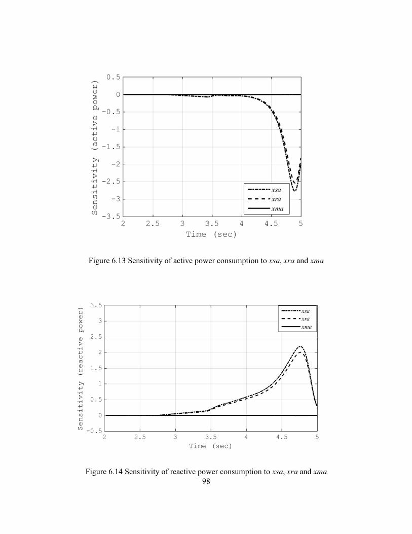
98
Figure 6.13 Sensitivity of active power consumption to xsa, xra and xma
Figure 6.14 Sensitivity of reactive power consumption to xsa, xra and xma
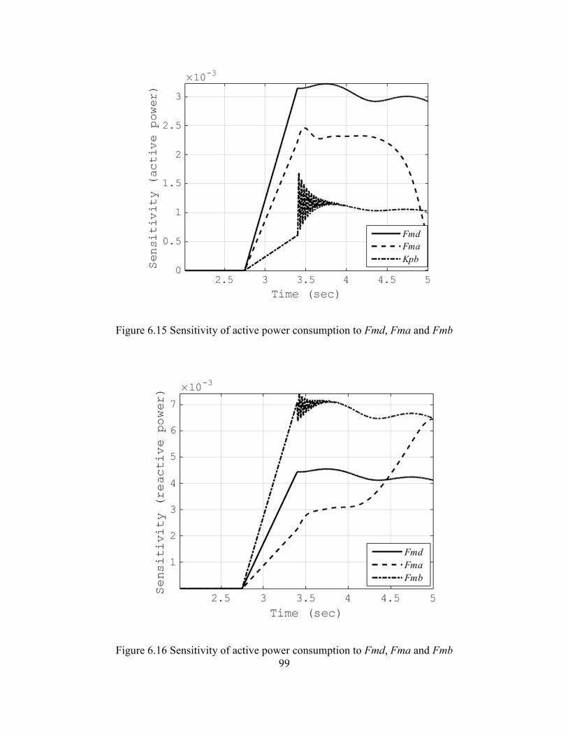
99
Figure 6.15 Sensitivity of active power consumption to Fmd, Fma and Fmb
Figure 6.16 Sensitivity of active power consumption to Fmd, Fma and Fmb
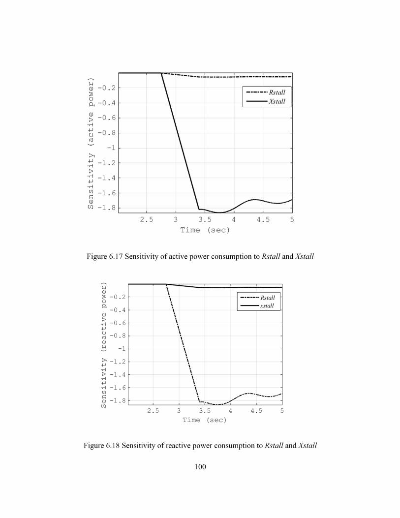
100
Figure 6.17 Sensitivity of active power consumption to Rstall and Xstall
Figure 6.18 Sensitivity of reactive power consumption to Rstall and Xstall

101
For nonlinear least squares problem, with an ill conditioned JtJ, the Levenberg-
Marquardt algorithm is more efficient as compared to the Gauss-Newton method. Apart
from using a different algorithm, the sensitivity information can be used to make the pa-
rameter estimation process more efficient. The sensitivity of the active and reactive power
consumption of the composite load model to the parameters Fmd, Fma, and Fmb is much
less as compared to the physical parameters of the models like the stator and the rotor
impedance. Since the parameter vector is updated based on the gradient, the parameters
Fmd, Fma and Fmb would not change much from the initial guess with every iteration,
whereas the physical parameters of the model like xs, xr, rr, rs will change substantially.
This might result in the estimation tool returning unrealistic values for the physical param-
eters of the model. To avoid such error in this example, one approach consists of fixing the
values of the percentage of individual components of the composite load model based on
additional knowledge about the load and then estimate the remaining parameters of the
model based on the measurements. Another approach to avoid error in parameter estima-
tion is to set appropriate upper and lower bounds on the parameters. A method for imple-
menting parameter bounds while using the Levenberg-Marquardt method is given by (6.8)
and (6.9). The parameter xm does not have any impact on the active or reactive power
consumption of the model. This parameter can be fixed at the beginning of the estimation
process. For parameters like xr and xs, whose sensitivities are linearly dependent, a fixed
ratio could be assumed between these two parameters as given by
xs
xrxr =δ ,
(6.10)
where, δxr is the increment in xr corresponding to an increment in xs.

102
6.3.2 Parameter estimation with reduced number of parameters
Based on the analysis presented in the previous section the parameter estimation
process is repeated by fixing certain parameters of the model. The parameters Fmd, Fma,
Fmb, and xm are fixed before the estimation process. Table 6.6 shows the values of the
fixed parameters for the reduced parameter estimation process. Since this is a test example,
the parameters are kept close to the values obtained in Table 6.5. The ratio between xs and
xr is fixed to 8 for motor A and 4 for motor B. The initial guess for the remaining parame-
ters are kept the same as given in Table 6.3. As the number of parameters is reduced, the
parameter estimation process is faster, since the dimensions of the optimization problem is
reduced. Furthermore, with the reduced set of parameters the condition number of JtJ is
2286, which shows that the reduced problem is not ill-conditioned. The problem can now
be solved easily using the Gauss-Newton algorithm in lsqnonlin. Figure 6.21 and Figure
6.22 show the measured as well as the fitted active and reactive power. The estimated com-
posite load parameters are listed in Table 6.4. The parameters that were fixed in the begin-
ning of the estimation process are marked in bold italics.
Table 6.7 Fixed values of parameters used in the reduced parameter estimation process
Parameter Fixed value
Fma 6
Fmb 12
Fmd 62
xma 3 pu
xmb 3 pu
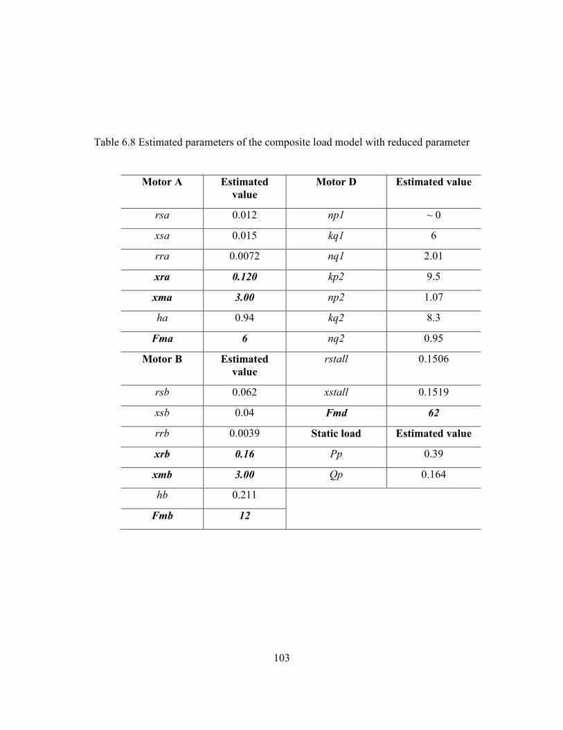
103
Table 6.8 Estimated parameters of the composite load model with reduced parameter
Motor A Estimated
value
Motor D Estimated value
rsa 0.012 np1 ~ 0
xsa 0.015 kq1 6
rra 0.0072 nq1 2.01
xra 0.120 kp2 9.5
xma 3.00 np2 1.07
ha 0.94 kq2 8.3
Fma 6 nq2 0.95
Motor B Estimated
value
rstall 0.1506
rsb 0.062 xstall 0.1519
xsb 0.04 Fmd 62
rrb 0.0039 Static load Estimated value
xrb 0.16 Pp 0.39
xmb 3.00 Qp 0.164
hb 0.211
Fmb 12
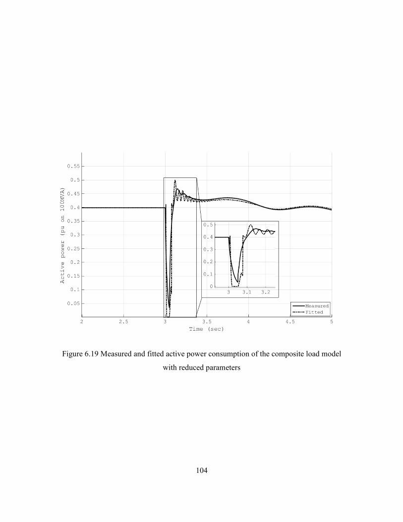
104
Figure 6.19 Measured and fitted active power consumption of the composite load model
with reduced parameters
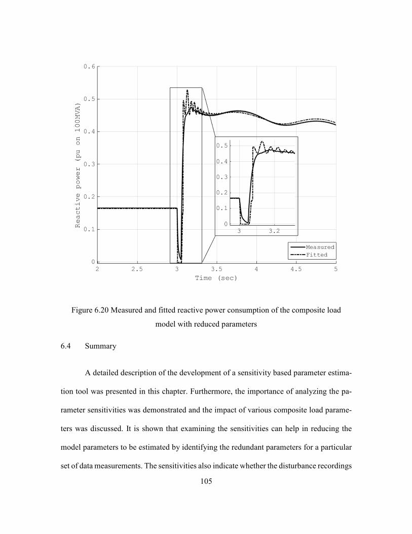
105
Figure 6.20 Measured and fitted reactive power consumption of the composite load
model with reduced parameters
6.4 Summary
A detailed description of the development of a sensitivity based parameter estima-
tion tool was presented in this chapter. Furthermore, the importance of analyzing the pa-
rameter sensitivities was demonstrated and the impact of various composite load parame-
ters was discussed. It is shown that examining the sensitivities can help in reducing the
model parameters to be estimated by identifying the redundant parameters for a particular
set of data measurements. The sensitivities also indicate whether the disturbance recordings

106
are sufficient to identify the parameters of interest uniquely. In addition, an example of
parameter estimation was presented here. The parameters of a positive sequence composite
load model were estimated from a surrogate disturbance measurement recorded from an
electromagnetic transient simulator.

107
CHAPTER 7: CONCLUSIONS AND FUTURE WORK: LOAD SENSITIVITY
STUDY
7.1 Conclusions
Load modeling is an important aspect of performing time-domain stability studies
for transmission system planning and operations. Due to the stochastic nature of the load,
one of the key challenges in load modeling is determining the composition and the aggre-
gate model parameters. Sensitivity analysis provides a systematic approach to analyze the
effect of load parameter uncertainty on the power system response. In the work presented
in this dissertation, TS analysis was used to study the impact of load model parameter
uncertainty on the power system response. However, the present day commercial power
system simulators do not have the capability to perform TS analysis. To this end, the im-
plementation of TS analysis was presented using an explicit integration method, which is
commonly used in all commercial simulators. In addition, a TS analysis was implemented
in GE-PSLF using a numerical method. The chapter further discusses some of the draw-
backs of using a numerical method for TS analysis when non-smooth load models are used.
Chapters 2 to 5 of this dissertation document the work done on the application of TS anal-
ysis in load modeling.
Due to the aggregated nature of the load models, parameter estimation is a chal-
lenging task in load modeling. Sensitivity analysis can be used to perform load model
parameter estimation in a much more efficient and insightful manner. Chapter 6 presents
the development of a sensitivity based parameter estimation tool. Furthermore, a discussion
on utilizing the sensitivities to identify the suitability of the measurement and parameter

108
redundancy is presented in chapter 6. The main conclusions of the work presented in chap-
ter 2 to chapter 6 are as follows:
1. A TS based method estimates the change in system response due to a change
in a parameter by a linear approximation. Therefore, this method allows a
planner to study multiple scenarios with uncertain load parameters without
the need of multiple TDS.
2. To evaluate the trajectory sensitivities, a single linear matrix equation needs
to be solved in addition to the computation required for the TDS. Further-
more, the factors of the coefficient matrix in the linear matrix equation are
obtained as a by-product of the TDS procedure. Hence, the TS based
method enables considerable savings in computation time while analyzing
the impact of parameter uncertainty.
3. The computation of individual parameter sensitivities are independent from
each other and can be done in parallel. Parallel computation of various sen-
sitivities enables further savings in computation time.
4. It was shown that the different parameters in the load model have markedly
different effect on the behavior of the system. Parameter sensitivities help
the planner/operator to understand the contribution of different parameters
to the system response. Parameters like Vstall and Tstall, which effect the
time instant and the duration required for a SPIM to stall, affect the system
very differently from parameters like Rstall, Xstall and Fmd.

109
5. The linear estimates of the actual system variable trajectories were found to
be reasonably accurate for small perturbations in parameter size.
6. Although the perturbation size for linear accuracy has been explored for
continuous equipment models, the non-smooth behavior of the load models
was found to impose additional constraints on the parameter perturbation
size.
7. The error introduced due to the non-smooth nature of the load is primarily
localized in nature. However, the impact on the trajectory estimation in
other parts of the system is dependent on the magnitude of the discrete
change caused by the switching event in the non-smooth load model.
8. The computation of the maximum perturbation size considering a switching
event can be framed as BVP and can be solved using the shooting method.
The formulation of the problem does not require any additional computa-
tion. However, the shooting method is an iterative procedure, requiring mul-
tiple TDS.
9. The TS analysis can be implemented using an explicit integration routine.
However, additional computational effort is required to perform TS analysis
and the entries of the linear matrix equation required to compute the sensi-
tivities are not available as a byproduct of the TDS routine.
10. Although additional computation is required, the entire process of estimat-
ing the perturbed trajectories using an explicit integration may not require

110
more computation time as compared to implicit integration based TS anal-
ysis. The computation time depends on the problem and the time step of
integration used.
11. TS analysis can be implemented using present day commercial power sys-
tem simulators using a numerical finite differencing method. This can be
done irrespective of the integration method employed in the power system
simulator as the trajectories are computed numerically. However, the nu-
merical approach is not suitable for computing the maximum perturbation
size when non-smooth load models are used.
12. Parameter sensitivities provide useful insight into the measurement based
parameter estimation process. An inspection of the Jacobian matrix can re-
veal whether the measurements made are sufficient to estimate all the pa-
rameters of interest. Furthermore, the Jacobian entries convey information
as to whether two or more parameters have similar impact on the measure-
ments used for parameter estimation. In this case, it is difficult to identify
the parameters uniquely as the estimation problem is ill conditioned.
13. Based on the parameter sensitivities the dimension of the parameter estima-
tion problem can be reduced by fixing the values of some redundant param-
eters. Sensitivity analysis enables the identification of the redundant param-
eters for a particular disturbance measurements used.
111
7.2 Future work
The findings of the study highlight the importance of adopting sensitivity-based
techniques in mainstream analysis. In terms of the application of TS analysis in load mod-
eling studies, the future work includes implementation of this module in a commercial
power system simulator. An implementation of the TS analysis is shown here using an
explicit integration algorithm, which is most commonly used in commercial power system
simulators. However, as the formulation of the TDS routines in commercial simulators is
different from PSAT, further work is needed for commercialization of the TS module
For sensitivity based parameter estimation, the results presented in this work are
based on surrogate measurements made from simulations performed in EMTDC/PSCAD.
The next step would be to use actual disturbance recordings for parameter estimation. It
was shown that the disturbance measurements might not be sufficient to identify all the
parameters of the load model uniquely. The sensitivity-based approach can be utilized to
determine the type of disturbance measurements that may be needed to identify all the
parameters in the composite load model. Furthermore, if a particular type of disturbance is
of interest, the sensitivity-based approach can also be utilized to derive a reduced parameter
load model. These areas of parameter estimation can greatly improve load modeling and
require further research.

112
CHAPTER 8: POWER SYSTEM SECURITY ASSESSMENT FOR N-1-1 CON-
TINGENCIES
Power system security is the ability to maintain uninterrupted supply of power from
the generation sources to the load centers, especially when subjected to a disturbance [21],
[60], [61]. Disturbances could be due to faults in the system resulting in the loss of a line
or generator or simply due to scheduled maintenance activities by utilities [61]. Such
events, leading to the loss of lines/transformers or generators are termed as contingencies.
Power system security assessment deals with examining whether the system is capable of
serving the loads after the occurrence of such contingencies.
The September 2011, blackout in San Diego and parts of the southwestern U.S. has
highlighted the need to examine n-1-1 contingencies in which, the second outage is not
related or dependent on the initiating outage [18], [17]. The identification of critical n-1-1
contingencies is an important step in the planning process. It helps the utilities to identify
and plan for IROLs, which may affect the system operating limits [18]. The work done in
this part of the report proposes a systematic approach to n-1-1 security assessment consid-
ering both steady state as well as the dynamic response of the system. In the following
sections, key concepts related to power system security assessment are introduced and the
need for a new approach is highlighted.
8.1 Contingency analysis
Contingency analysis serves as a tool to assess, whether a power system can be
operated within security limits after the occurrence of planned or unplanned outages [62].
An n-1 contingency analysis involves, studying the impact of outage of a single component

113
on the system voltages and the branch flows [18], [60]. Similarly, an n-k contingency anal-
ysis involves studying the impact of simultaneous outage of k components on the system
voltages and the branch flows [18], [60]. For n-1-1 contingency analysis, the two contin-
gencies are applied sequentially rather than simultaneously. System adjustments if needed
are made after the first outage, prior to applying the second outage [18]. An n-1-1 contin-
gency differs from an n-2 (n-k with k = 2) contingency in the manner the two outages are
simulated.
8.2 Power system security assessment
Power system security assessment can be broadly classified into two categories,
namely static security assessment (SSA) and dynamic security assessment (DSA) [21],
[60], [61]. Both the steady state performance and the transient behavior of the system need
to be accounted for in determining the system operating thresholds [17].
Static security assessment (SSA) deals with examining whether the post-contingent
steady state operating state is acceptable from a power system operations viewpoint [21],
[60]. A post-contingent operating state is acceptable when all bus voltages in the system
are within an allowable range and all transmission lines and transformers are loaded within
their short-term emergency limits. During SSA, it is assumed that the fast acting controls
in the system have acted and reached a steady state and the slow acting controls and human
actions have not responded yet. Multiple power-flow analyses are performed for different
contingencies to compute the post-contingent system voltages and branch flows. The volt-
ages and branch flows are then compared with set thresholds to gauge the severity of the
outages.
114
Dynamic security assessment (DSA) on the other hand deals with examining the
transition of the system from the old equilibrium point to the new equilibrium point fol-
lowing the outage [21], [60]. If the transition is stable and the new equilibrium point is
acceptable from a system operations viewpoint the contingency is termed secure and oth-
erwise insecure [63]. TDS is the method of choice while performing DSA. The outages are
simulated as a disturbance and the evolution of the system variables are recorded to deter-
mine whether the system is stable. DSA takes into account the behavior of slow and fast
acting controls in the system during a disturbance.
A traditional approach to power system security assessment is to inspect all possible
contingencies sequentially, and study their impact on the steady state and transient perfor-
mance of the system [64].This process entails performing multiple power flows for SSA
and multiple TDS for DSA to cover all possible contingencies. However, for any well-
designed power system, not all contingencies are harmful. To save computation time, it
befits a planner or an operator to inspect a smaller subset of contingencies that are deemed
critical from a system security viewpoint [64]. If such a subset is chosen solely based on
the operator’s or the planner’s experience, some critical cases might be omitted in the pro-
cess. To solve the problem of identifying critical contingencies various contingency screen-
ing methods have been reported in literature for both SSA and DSA. The contingency
screening methods rely on performing approximate computations to identify the severe
contingencies before proceeding to a more detailed evaluation. The following subsections
present a review of the contingency screening methods presented in literature for SSA and
DSA.
115
8.2.1 Contingency screening for SSA in power systems
The contingency screening and ranking methods presented in the literature for SSA
can be broadly classified under explicit methods and implicit methods. Explicit methods
for contingency screening define system-wide performance indices (PIs), which capture
the voltage and line flow violations, in the system [64, 67-70]. After the appropriate PIs
have been defined, the first order sensitivities of the PIs are computed with respect to pa-
rameter changes. For outage studies the power system components are modeled to include
parameters, which when changed can simulate the outage of the component. References
[67-70] describe different modeling approaches for contingency analysis using explicit
methods. The magnitude of the first order PI sensitivities to these parameters, serve as
indicators of severity and are used to rank the contingencies. References [64, 67-70], lists
the various indices that have been developed to rank contingencies using explicit methods.
Once the contingencies are ranked in the order of their severity, the top-ranking contingen-
cies are classified as critical. The main drawback of explicit methods is that the PIs defined
are highly nonlinear functions of the system parameters [70]. Screening based on the first
order sensitivities around a base case often results in inaccurate assessment of contingen-
cies. Moreover, inclusion of additional nonlinearities like load tap changers, generator re-
active power limits and nonlinear load models amplify the error associated with contin-
gency screening and ranking [70].
Implicit methods for contingency screening use network solutions to identify volt-
age and flow violations [65, 56, 71-75]. In the past, due to computational limitations, these

116
methods have traditionally relied on approximate or partial post-contingent network solu-
tions to estimate the line flows and the bus voltages. Branch overloads could be typically
identified by performing dc power-flow and only solving relevant portions of the network
[66, 73]. Single iterations of fast-decoupled power flow have been used to estimate the
post-contingent system voltages [73]. It is assumed that the effect of a contingency is lo-
calized in nature and hence methods have been proposed to find localized solutions to as-
sess the severity of the contingency [71]. Methods have also been proposed to approximate
the widespread effects of contingencies along with the local effects [72, 73]. Such methods
use sparsity oriented compensation techniques along with partial re-factorization methods
to achieve computational efficiency [75]. Although fast, implicit methods can potentially
underestimate the widespread effects of contingencies due to the approximations involved.
8.2.2 Contingency screening for DSA in power systems
It is worthwhile to mention that DSA, as discussed in various literatures, primarily
deals with evaluating whether a system is able to maintain stability after large disturbances
such as a fault on a line and the corresponding protection system action [76-79]. Although,
generator outages are a part of DSA, such outages do not pose any immediate threat to the
system from a rotor angle stability point of view. As rotor angle stability is being discussed
here, analysis of generator outages have not been pursued in this report.
Various contingency screening methods for DSA have been proposed in literature
[77-84]. A coherency-based index for contingency screening is described in reference [79].
References [77-82], describe contingency screening techniques based on the transient en-
ergy function. Filtering of contingencies using sparse transient energy function is described
117
in [80, 81]. Extensions of static security analysis techniques coupled with applications of
artificial neural networks have also been explored for contingency screening and ranking
[83]. Composite indices based on coherency, transient energy conversion and dot products
have been proposed for contingency screening [84]. Most of these screening methods com-
pute the required indices by performing short duration time domain simulations only until
a few cycles after the disturbance.
8.3 Need for a new contingency screening and ranking method for n-1-1 contingencies
As presented in the preceding section, contingency analysis is a mature field and
various screening methods for n-1 contingency analysis have been proposed for both SSA
and DSA. However, applying these techniques for n-1-1 contingencies can be problematic.
For SSA, the explicit and the implicit contingency screening methods reported in literature
have been verified on smaller test systems for single (n-1) branch or generator outages.
However, since the described methods rely on first order sensitivities or partial network
solutions, they might fail to capture the effect of multiple outages, which can be highly
nonlinear [85], [86]. Therefore, these methods cannot be reliably extended to n-1-1 contin-
gency analysis [87]. Similarly, for DSA, screening n-1-1 contingencies using the traditional
screening methods can also be impractical [87]. This is due to the staggering number of
short duration TDS that need to be performed [87]. To address the problems with reliability
and accuracy, a new approach for n-1-1 contingency screening and ranking is needed for
both SSA and DSA [87]. To this end, this report proposes
1. A method to screen and rank n-1-1 contingencies for static security assess-
ment (SSA), and

118
2. A method to screen and classify n-1-1 contingencies for dynamic security
assessment (DSA).
Both the proposed methods are intended to be used during the planning phase by
planners or operators. One of the important features of the proposed methods is that these
methods can be implanted easily with any existing power system simulator without the
need of any additional investment.
8.4 Summary
This chapter presented some of the key concepts of contingency analysis for SSA
and DSA. A literature survey of the existing methods of contingency screening and ranking
for both SSA and DSA is presented here. In addition, the need for a new approach for n-1-
1 contingency screening and ranking is highlighted in this chapter.
119
CHAPTER 9: N-1-1 CONTINGENCY SCREENING AND RANKING FOR SSA
The majority of contingency screening and ranking methods rely on linear sensitiv-
ities or partial local solutions of the network to gauge the severity of the outage. Chapter 8
provided a review of methods that have been proposed in the literature. However, the effect
of severe contingencies on bus voltages and branch flows can be highly nonlinear and
hence, approximate methods often fail to assess the criticality of severe contingencies. The
approximation errors can be substantial for n-k (for k > 1) or n-1-1 contingencies.
With the advancement in computational capabilities in terms of hardware, it is pos-
sible to perform complete power-flow solutions in a reasonable time for large power sys-
tems. It is therefore convenient to use ac power solutions to develop reliable filters to screen
and rank contingencies. Such methods have already been adopted in some commercial
power system simulators [22], [23]. This chapter describes an existing n-1-1 contingency
screening method in a commercial power system simulator and proposes a novel n-1-1
contingency screening and ranking methodology based on full ac power-flow solutions.
The proposed screening and ranking method is designed such that it can be easily imple-
mented with any commercial power system simulator with relative ease. The commercial
power system simulator used for this work is GE-PSLF [22].
9.1 Existing method for n-1-1 contingency screening in GE-PSLF
The SSTools module in GE-PSLF has an inbuilt routine to generate a list of
screened n-1-1 contingencies [22], [88], [89]. This routine creates a list of n-1-1 contin-
gencies based on a severity index that is computed from the results of the n-1 contingency
analysis [88], [89]. A brief description of the method is as follows [88], [89]:

120
3. Power-flow solutions are performed for all n-1 cases. The bus voltages and
the branch flows are recorded for every outage at user-specified locations
in the system. Locations refer to the specific areas or zones within a power
system.
4. The branch flows and the bus voltages for each contingency are compared
against the user-defined thresholds. These thresholds could be:
a. The maximum and minimum allowable voltage levels
b. The change in voltage from pre-contingent condition
c. The maximum allowable flow on a branch (line or transformer)
d. The change in branch flows from pre-contingent condition
e. A combination of (a) and (b) for bus voltages and (c) and (d) for
branch flows
5. The severity index for a contingency is incremented by 1 for each branch
flow violation or voltage violation. Depending on the number of violations
due to an outage, the severity index of the n-1 contingency is computed.
6. Once the severity index for each n-1 contingency is computed, all n-1 con-
tingencies with severity index greater than a user-defined value are consid-
ered for n-1-1 analysis. The n-1-1 contingency list is created by forming all
possible combinations of the screened n-1 contingencies.
The above-described method in SSTools seeks to identify n-1-1 contingencies
based on the assumption that if two contingencies individually cause voltage or branch
flow violations, the combination of such contingencies can be critical. All combinations of
contingencies, which do not cause voltage or flow violations individually, will be ignored

121
by this screening process. However, some combinations of innocuous contingencies oc-
curring as an n-1-1 contingency can be potentially harmful. Such instances of inadequacy
of the existing method were observed while analyzing the WECC. The WECC system has
20605 buses, 17056 lines, 7836 transformers and 2737 generators. An example of such a
case for the WECC system is as follows:
Case: The outage of the branches 2320-2319 and 2322-2319
A schematic one-line diagram of the region of interest is shown in Figure 9.1. The
two branches to be disconnected are marked with dotted crosses. Table 9.1 lists the voltages
at some selected buses in the region for the base case and following the individual outages
of the marked branches. From Table 9.1, it can be seen that the individual outages do not
have a considerable impact on the bus voltages. However, when these contingencies are
considered sequentially, severe undervoltages are observed at those buses. Table 9.2 lists
the voltages at the load buses due to the sequential outage of the two branches.
When either the branch 2322-2319 or the branch 2320-2319 is disconnected, the
power supply to the load area is simply re-routed through the remaining line in service
when the other one is disconnected. However, when both these marked lines are discon-
nected sequentially, the loads in the region are supplied through the only alternate path
2320-1720-1721. The alternate path, marked by a dotted line in Figure 9.1, has considera-
bly higher impedance. The large voltage drop on the higher impedance path and lack of
reactive power resources in the region leads to depressed voltages at the load buses.
This example illustrates that the method of screening contingencies based on the
impact of individual contingencies may not be sufficient for screening n-1-1contingencies.
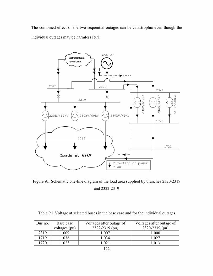
122
The combined effect of the two sequential outages can be catastrophic even though the
individual outages may be harmless [87].
Figure 9.1 Schematic one-line diagram of the load area supplied by branches 2320-2319
and 2322-2319
Table 9.1 Voltage at selected buses in the base case and for the individual outages
Bus no. Base case
voltages (pu)
Voltages after outage of
2322-2319 (pu)
Voltages after outage of
2320-2319 (pu)
2319 1.009 1.007 1.000
1719 1.036 1.034 1.027
1720 1.023 1.021 1.013

123
1721 1.017 1.015 1.007
Table 9.2 Voltage at selected buses for the sequential outage of the two branches
Bus no. Voltages after outage of 2322-2319
and 2320-2319 (pu)
2319 0.85
1719 0.86
1720 0.87
1721 0.87
9.2 Contingency screening for n-1-1 analysis
In a well-planned interconnected power system, the outage of a single component
only affects a few branch flows and generator outputs. The majority of branch flows and
generator outputs throughout the system remain practically unchanged. It can be intuitively
observed that substantial changes in the branch flows or the generator outputs following an
outage indicate that the affected branches and/or generators compensate for the discon-
nected component. Therefore, to account for the critical n-1-1 contingencies, the candidate
branches or the generators for the second outage can be screened by analyzing their pre-
contingent and post-contingent state (flows for branches and outputs for generators) fol-
lowing the first outage. The following sub-sections describe the methods to generate an n-
1-1 contingency list for branch-branch, generator-branch, and generator-generator outages
with examples and explanations.
9.2.1 Contingency screening for branch-branch outages
To generate a list of n-1-1 contingencies involving branch-branch outages, the fol-
lowing steps are followed [87]:

124
1. Perform a full ac power-flow for all n-1 branch contingencies and store all
the branch MVA flows.
2. For each branch outage, compute the percentages of MVA flow in the dis-
connected branch that shows up in all other branches in the system. This
percentage is the ac equivalent of the line outage distribution factor (LODF)
and will be referred to as ACLODF in the rest of this report. As an example,
the ACLODF in a hypothetical line A for outage of line B is computed as
follows:
100,
,,1
−= −
bbase
AbaseABn
ABMVA
MVAMVAACLODF , (9.1)
where,
ACLODFAB is the percentage of MVA flow in line B that shows up on line
A.
MVAn-1,AB is the MVA flow on line A with line B disconnected.
MVAbase,A is the MVA flow on line A in the base case ( all lines in service).
MVAbase,B is the MVA flow on line B in the base case ( all lines in service).
3. All branches that have an ACLODF more than a set threshold for an n-1
contingency are screened as candidate branches for the second outage fol-
lowing that particular n-1 contingency.
4. The n-1-1 contingency list is updated to include all pairs of the n-1 outage
and the corresponding screened second outages in step 3. Steps 2 to 4 are
performed for all n-1 contingencies.

125
5. For every candidate branch screened in step 3, the MVA flow on that branch
due to a combination of any two n-1 outage is estimated. The change in flow
is linearly approximated by using the already computed ACLODFs.
6. The contingency list is updated to include any combination of two n-1 con-
tingencies, which may cause the estimated flow on a screened branch com-
puted in step 5, to be above a set percentage of the emergency rating of the
branch.
7. Finally, all duplicate n-1-1 contingencies are removed from the list and the
final list of n-1-1 contingency is printed out in GE-PSLF SSTools format.
An example is provided here to illustrate steps 3 to 6. It should be noted that the
example is intended to highlight the screening process once an n-1 analysis is completed.
It is purely demonstrative and numbers quoted are for the sake of illustration. Consider a
power system example with lines designated as 'line 1', 'line 2', 'line 3' and so forth. Figure
9.2 shows the list of screened branches due to some n-1 branch outages. The ACLODF of
each branch due to the corresponding n-1 branch outage is listed on top of the branch name.
It can be seen that the list contains branches with ACLODF more than 10 percent. The
threshold for screening mentioned in step 3 is set to be 10 percent in this example. The
intermediate n-1-1 contingency list formed in step 4 is shown in Figure 9.3.
It is assumed that for line 3 in Figure 9.2 the sum total of the base flow and the
change in MVA flow due to the outages of line 1 (10.2 percent) line 4 (11.5 percent) is
more than 80 percent of its emergency rating. Hence, as indicated in step 6 the combination

126
of outage of line 1 and line 4 is added to the list. Figure 9.4 shows the updated n-1-1 con-
tingency list.
After all the contingencies are added to the list, the duplicate n-1-1 contingencies
are removed and the final list of contingencies is created. Figure 9.5 shows the final list of
n-1-1 contingencies with the duplicate contingencies removed. The duplicate entries are
outlined and the removed entries are marked with a cross sign beside them.
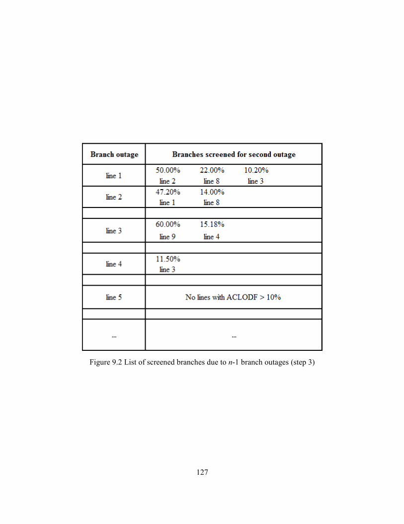
127
Figure 9.2 List of screened branches due to n-1 branch outages (step 3)
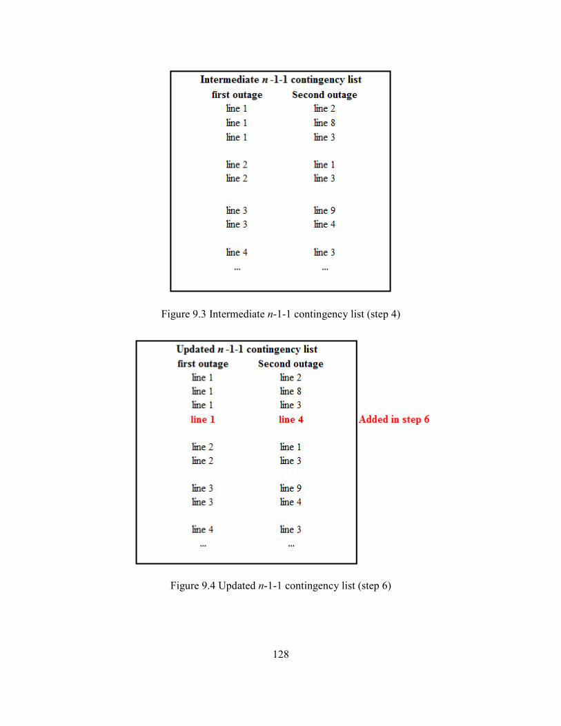
128
Figure 9.3 Intermediate n-1-1 contingency list (step 4)
Figure 9.4 Updated n-1-1 contingency list (step 6)
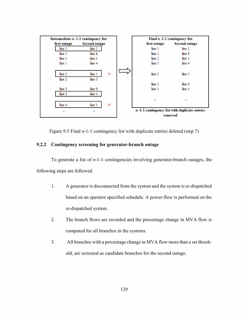
129
Figure 9.5 Final n-1-1 contingency list with duplicate entries deleted (step 7)
9.2.2 Contingency screening for generator-branch outage
To generate a list of n-1-1 contingencies involving generator-branch outages, the
following steps are followed.
1. A generator is disconnected from the system and the system is re-dispatched
based on an operator specified schedule. A power-flow is performed on the
re-dispatched system.
2. The branch flows are recorded and the percentage change in MVA flow is
computed for all branches in the systems.
3. All branches with a percentage change in MVA flow more than a set thresh-
old, are screened as candidate branches for the second outage.

130
4. The n-1-1 contingency list is updated to include all pairs of the n-1 generator
outage and the corresponding screened second outages in step 3. Steps 2 to
4 are performed for all n-1 contingencies.
5. The contingency list is updated to include any combination of two n-1 gen-
eration outage, which may cause the estimated flow on a screened branch
computed in step 5, to be above a set percentage of the emergency rating of
the branch.
It should be noted that contingencies added in step 5 are essentially generator-gen-
erator contingencies. These contingencies could be omitted from here and later added to
the list of generator-generator contingencies. However, these contingencies, if any, were
added to the generator-branch contingency list for the purpose of this study. If any such n-
1-1 contingency re-appeared in the generator-generator contingency list, they were subse-
quently removed.
To illustrate the steps 3 to 5, consider the power system example of section 9.2.1.
The generators are numbered 'gen 1’, 'gen 2’, 'gen 3' and so forth. Figure 9.6 shows the
screened branches due to some n-1 generation outages. The percentage change in MVA
flow on a branch due to the corresponding n-1 generation outage is listed on top of the
branch name. It can be seen that the list contains branches with a percentage change in
MVA flow more than 10 percent. The threshold mentioned in step 3 is set at 10 percent for
this example. The intermediate n-1-1 contingency list formed in step 4 is shown in Figure
9.7.

131
It is assumed that for line 5 in Figure 9.6 the sum total of the base flow and the
change in MVA flow due to the outages of gen 2 (28.5 percent) gen 4 (11.5 percent) is
more than 80 percent of its emergency rating. Hence, as indicated in step 5 the combination
of outage of gen 2 and gen 4 is added to the list. Figure 9.8 shows the final n-1-1 contin-
gency list with the updated entries.
Figure 9.6 List of screened branches due to n-1 generator outage (step 3)
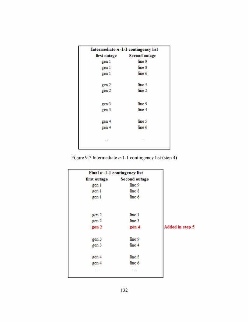
132
Figure 9.7 Intermediate n-1-1 contingency list (step 4)

133
Figure 9.8 Final n-1-1 contingency list (step 5)
9.2.3 Contingency screening for generator-generator outage
To generate a list of n-1-1 contingencies involving a generator-generator outage,
the following steps are followed.
1. A generator is disconnected from the system and the system is re-dispatched
based on an operator specified schedule. A power-flow is performed on the
re-dispatched system.
2. From the power-flow solution of the n-1 analysis, the reactive power gen-
eration of each generator is recorded.
3. The generators, which have a reactive power increase of more than a set
threshold, are screened as candidate generators for the second outage.
4. Generators, which are on their upper or lower reactive power limits follow-
ing the n-1 generator outage and re-dispatch are also screened as candidate
generators for second outage
5. The n-1-1 contingency list is updated to include all pairs of the n-1 generator
outage and the corresponding screened second outages in step 3. Step 2 to
step 4 is performed for all n-1 contingencies.
6. The duplicate contingencies are removed after the list is formed.
To illustrate steps 3 to 5, consider the power system example of Section 9.2.1. Fig-
ure 9.9 shows the screened generators due to some n-1 generator outages. The percentage
change in reactive power output is listed on the top of the generator names. The threshold
mentioned in step 3 is set at 10 percent for this example. Hence, generators with a change

134
in reactive power output of more than 10 percent are screened as candidate generators for
a second outage. Figure 9.9 also lists the generators that are at their maximum and mini-
mum reactive power limits.
Figure 9.10 shows the intermediate n-1-1 contingency list and Figure 9.11 shows
the final n-1-1 contingency list with duplicate entries removed. The duplicate entries are
outlined and the removed entries are marked with a cross beside them.
Figure 9.9 List of screened generators due to n-1 generator outage (step 3)

135
Figure 9.10 Intermediate n-1-1 contingency list (step 5)
Figure 9.11 Final n-1-1 contingency list with duplicate entries deleted (step 6)

136
9.3 Justification for the contingency screening method
The contingency screening method proposed in the previous section is expected to
screen possibly critical second outages following an n-1 outage. The screened n-1-1 out-
ages may cause voltage or branch flow violations in the system. This section provides an
explanation of how the screening method identifies n-1-1 contingencies that might be crit-
ical from a system operation point of view.
For branch-branch outages, if the outage of a single branch causes the ACLODF for
another branch to be significantly high, it indicates that this second branch is an important
supply route to the same load area. An outage of a branch with a high ACLODF can lead
to considerable weakening of the transmission path to a load area. The alternate supply
route to the load may have substantially higher impedance. This can lead to large voltage
drops and possible reactive power problems at the load buses. Close to large generation
sources, disconnecting a branch with high ACLODF can cause significant reduction in the
short circuit ratio, leading to stability issues. Hence, the outage of such a branch may be
critical following the corresponding n-1 branch outage. Furthermore, if two separate n-1
branch outages cause the estimated MVA flow on a branch or branches to increase beyond
its emergency rating, the sequential combination of the two n-1 outages can also be critical.
This is particularly significant in identifying n-1-1 contingencies that resulted in overload-
ing of transformers and lines, which were operating near their emergency ratings in the
base case. Steps 3 to 6 in the algorithm presented in section 9.2.1 screen n-1-1 branch-
branch outages based on these ideas.

137
For generator-branch outages, if the outage of a generator causes a significant in-
crease in MVA flow on a branch, it indicates that a part of the lost reactive power in the
area is being imported through this branch. Outage of such a branch may cause voltage
violations in the load areas. Hence, the outage of such a branch may be critical following
the corresponding n-1 generator outage. Furthermore, if two separate n-1 generator outages
cause the estimated MVA flow on a branch or branches to increase beyond its emergency
rating, the sequential combination of the two n-1 outages can also be critical. Steps 3 to 5
in the algorithm presented in section 9.2.2 screens n-1-1 generator-branch outages based
on these ideas.
For generator-generator outages, if the outage of a generator causes the reactive
power output of another generator to increase significantly, it indicates that a part of lost
reactive power is being supplied by this generator. Outage of such a generator may cause
voltage violations due to reactive power shortage. Hence, the outage of such a generator
may be critical following the corresponding n-1 generator outage. Furthermore, all gener-
ators that reach their reactive power limits following the outage of a generator are also
included for n-1-1 screening. Since these generators are at their reactive power limits dis-
connecting these generators from the system can lead to voltage violations at their regulated
buses. Steps 3 to 5 in the algorithm presented in section 9.2.3 screens n-1-1 generator-
generator outages based on these ideas.
9.4 Ranking of screened n-1-1contingencies based on severity
Ranking contingencies based on their severity enables a planner or an operator to
identify the most critical elements in a power system. Additional measures can then be

138
taken for hardening such elements to prevent future outages. Various indices have been
proposed to rank contingencies based on the severity of their impact on the system voltages
and the branch flows [64], [66], [70]. For the analysis presented in this report, performance
indices as defined in reference [64] are used. The voltage-based index and the flow-based
index are defined as follows:
Voltage based index
The voltage-based index ranks the contingencies based on the magnitude of the
voltage violations and the number of buses in the system where such violations occur [64].
The voltage-based index is defined by:
α
α
2
lim1 2
∆
−=∑
= i
sp
iinb
i
biV
V
VVwPI (9.2)
where,
PIV is the voltage-based index
nb is the total number of monitored buses in the system
Vi is the post-contingency voltage at a bus i
Visp is the nominal voltage at a bus i
∆Vilim is the maximum voltage change limit (normally 10 percent)
α is a factor that is usually chosen 1
wbi is a weighting factor
Flow based index

139
The flow-based index ranks the contingencies based on the magnitude of the flow
violations and the number of branches in the system where such violations occur [64]. The
flow-based index is defined by:
α
α
2
lim1 2
=∑
= i
inl
i
li
MVAS
SwPI (9.3)
where,
PIMVA is the flow-based index
nl is the total number of monitored branches in the system
Si is the post-contingency flow in branch i
Silim is the short term emergency rating of branch i
α is a factor that is usually chosen 1
wli is a weighting factor
The factor α used for ranking is usually assigned a value of 1 for both the voltage-
based and the flow-based index [64]. Due to the particular choice of this factor the indices
varies as a quadratic function of the voltage or flow violations.
The weighting factor wbi and wli in (9.2) and (9.3) respectively, are usually chosen
by an operator or a planner to assign higher weights to the critical buses or the critical lines
in the system. For example, if a particular line is important in a system and the overloading
of this line cannot be tolerated, the planner can assign a higher weight wli to that particular
line. If a contingency leads to overloading of this important line, the corresponding contin-
gency will have a higher value of the flow-based ranking index. Similarly, higher values
of wbi can be assigned to critical buses in the system, such that voltage violations at those
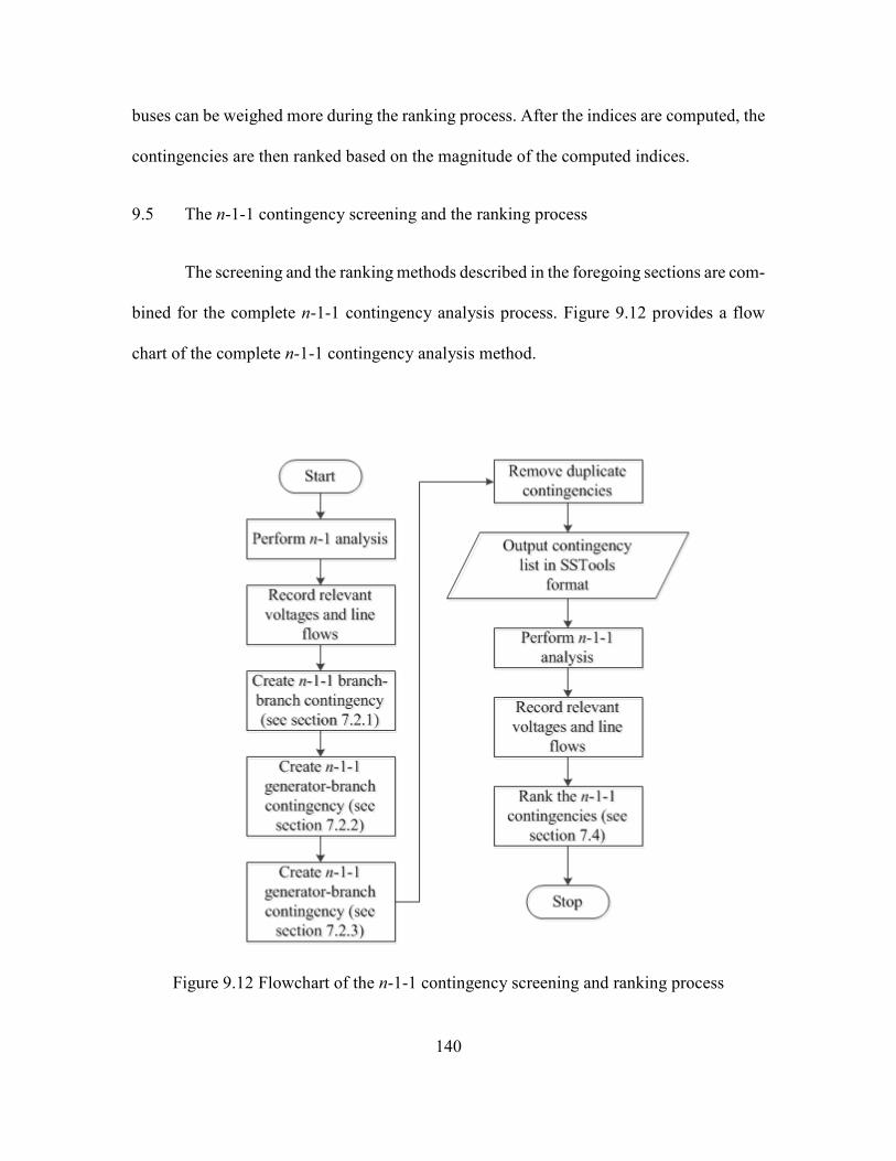
140
buses can be weighed more during the ranking process. After the indices are computed, the
contingencies are then ranked based on the magnitude of the computed indices.
9.5 The n-1-1 contingency screening and the ranking process
The screening and the ranking methods described in the foregoing sections are com-
bined for the complete n-1-1 contingency analysis process. Figure 9.12 provides a flow
chart of the complete n-1-1 contingency analysis method.
Figure 9.12 Flowchart of the n-1-1 contingency screening and ranking process

141
9.6 Summary
This chapter described the proposed contingency screening and ranking method for
n-1-1 contingency analysis. The proposed method systematically screens the critical n-1-1
contingencies thus reducing the number of n-1-1 contingencies to be processed. Once an
ac power-flow is performed for the screened n-1-1 contingencies, the contingencies can
then be ranked by the voltage-based and the flow-based index. In addition to the detailed
description of the screening and ranking methods, a flow chart for the complete n-1-1 con-
tingency analysis process is provided in this chapter.

142
CHAPTER 10: N-1-1 CONTINGENCY ANALYSIS FOR SSA: APPLICATION TO A
REAL SYSTEM
In chapter 9, a method for screening and ranking n-1-1 contingencies was proposed.
In this chapter, the proposed method is used to screen critical n-1-1 contingencies and rank
them for a real large power system. In the following sections, a brief description of the
power system used for this study is provided. The various thresholds used in the screening
and ranking process are defined and the results of the contingency analysis are presented
here. Furthermore, the accuracy of the proposed screening method is tested by performing
an exhaustive n-1-1 contingency analysis. The results of the comparative study are also
presented in this chapter.
10.1 System description
The proposed contingency screening and ranking method was used to perform n-1-
1contingency analysis for a selected utility within the WECC system. All voltage levels of
100 kV and above in the selected utility’s service area was considered for the contingency
analysis. A power flow file representing the entire WECC system, with detailed descrip-
tion of the selected utility’s service area was used for the study. Table 10.1 lists the key
features of the WECC system and the selected utility.
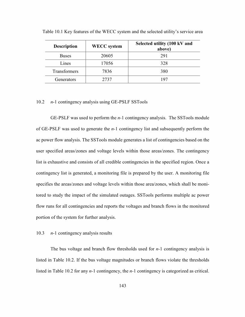
143
Table 10.1 Key features of the WECC system and the selected utility’s service area
Description WECC system Selected utility (100 kV and
above)
Buses 20605 291
Lines 17056 328
Transformers 7836 380
Generators 2737 197
10.2 n-1 contingency analysis using GE-PSLF SSTools
GE-PSLF was used to perform the n-1 contingency analysis. The SSTools module
of GE-PSLF was used to generate the n-1 contingency list and subsequently perform the
ac power flow analysis. The SSTools module generates a list of contingencies based on the
user specified areas/zones and voltage levels within those areas/zones. The contingency
list is exhaustive and consists of all credible contingencies in the specified region. Once a
contingency list is generated, a monitoring file is prepared by the user. A monitoring file
specifies the areas/zones and voltage levels within those area/zones, which shall be moni-
tored to study the impact of the simulated outages. SSTools performs multiple ac power
flow runs for all contingencies and reports the voltages and branch flows in the monitored
portion of the system for further analysis.
10.3 n-1 contingency analysis results
The bus voltage and branch flow thresholds used for n-1 contingency analysis is
listed in Table 10.2. If the bus voltage magnitudes or branch flows violate the thresholds
listed in Table 10.2 for any n-1 contingency, the n-1 contingency is categorized as critical.

144
Table 10.3 lists the voltage levels that are monitored for contingency analysis. While per-
forming ac power flow for contingency analysis, the following control actions were ena-
bled:
1. The load tap changers were set to adjust taps to regulate voltages.
2. The phase shifters were set to adjust phase angles to control the flow.
3. The static VAr devices were set to regulate voltages based on their control
types.
4. The area interchange was set to maintain the inter-area flows to the sched-
uled value.
Table 10.4 summarizes the n-1 contingency analysis results for the branch outages
obtained from SSTools. For the generator outage contingencies, the system was re-dis-
patched according to a schedule provided by the utility. Table 10.6 summarizes the n-1con-
tingency analysis results for the generation outages obtained from SSTools. From Table
10.5 and Table 10.6, it can be seen that 5 contingencies lead to voltage violations, 1 con-
tingency lead to a flow violation and for 1 contingency the power flow failed to solve. The
voltage and flow violations were observed in the system due to
1. Overvoltages at buses resulting from capacitive compensation from lightly
loaded lines
2. Overvoltages at buses resulting from the capacitive compensation from
fixed shunt devices
3. Existing undervoltage at buses in the base case

145
4. Overloading of parallel-connected transformer, when one of them is discon-
nected
The divergence of power flow can either be due to abnormal voltages in the system,
or due to unwanted operation of voltage and power flow control devices like under load
tap changers (ULTC), switchable reactor or capacitor banks and phase adjusters. Dead-
bands in discrete control devices can cause oscillations in the solution process without con-
vergence. Therefore, it is important to analyze the cases where the power flow solution
diverges or oscillates without reaching a solution. A method to analyze these cases is pre-
sented in a later section. In this particular case, the power flow solution diverges due to
severely depressed voltage in a load pocket close to the disconnected branch.
Table 10.2 Bus voltage and branch flow threshold for n-1 contingency analysis
Voltage and flow threshold for n-1 contingency ranking
Lower voltage threshold 0.95 pu
Upper voltage threshold 1.05 pu
Line flow threshold Short term emergency rating (rating 2 in GE-PSLF)
Table 10.3 Voltage and generation level selected for monitoring bus voltages and branch
flows and generator output
Voltage and generation level monitored for contingency
screening
Voltage 100kV - 500kV
Branch flows 100kV - 500kV
Generation All generators with output more than 50 MW
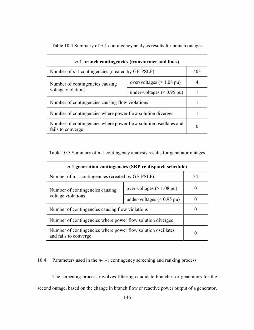
146
Table 10.4 Summary of n-1 contingency analysis results for branch outages
n-1 branch contingencies (transformer and lines)
Number of n-1 contingencies (created by GE-PSLF) 403
Number of contingencies causing
voltage violations
over-voltages (> 1.08 pu) 4
under-voltages (< 0.95 pu) 1
Number of contingencies causing flow violations 1
Number of contingencies where power flow solution diverges 1
Number of contingencies where power flow solution oscillates and
fails to converge 0
Table 10.5 Summary of n-1 contingency analysis results for generator outages
n-1 generation contingencies (SRP re-dispatch schedule)
Number of n-1 contingencies (created by GE-PSLF) 24
Number of contingencies causing
voltage violations
over-voltages (> 1.08 pu) 0
under-voltages (< 0.95 pu) 0
Number of contingencies causing flow violations 0
Number of contingencies where power flow solution diverges
Number of contingencies where power flow solution oscillates
and fails to converge 0
10.4 Parameters used in the n-1-1 contingency screening and ranking process
The screening process involves filtering candidate branches or generators for the
second outage, based on the change in branch flow or reactive power output of a generator,

147
following the first outage. The screening criteria are unique for each type of n-1-1 contin-
gency (branch-branch, generator-branch or generator-generator) and are described in later
sections separately. The ranking process is same for all n-1-1 contingency types. The volt-
age thresholds, the flow thresholds and the weighting factors used for the ranking process
are described in this section.
Table 10.6 lists the voltage and the flow thresholds used for the n-1-1 contingency
analysis. If the bus voltages or the branch flows violate the thresholds listed in Table 10.6
for any n-1-1 contingency, the n-1-1 contingency is categorized as critical. Based on the
thresholds given in Table 10.6, the weights wbi and wli of (9.2) and (9.3) are chosen. Table
10.7 lists the values of the weights wbi and wli used for ranking the n-1-1 contingencies.
The weights are chosen in such a way that non-zero performance indices be assigned to
only those n-1-1 contingencies, which cause violations in the system.
Table 10.6 Bus voltage and branch flow thresholds for n-1-1 contingency analysis
Voltage and flow thresholds for n-1-1 contingency ranking
Lower voltage threshold 0.90 pu
Upper voltage threshold 1.08 pu
Line flow threshold Short term emergency rating (rating 2 in PSLF)

148
Table 10.7 Choice of weights wbi and wli for n-1 contingency analysis
Weights for voltage based ranking
Bus voltage limit Value of wbi
Between 0.9 pu and 1.08 pu 0
Greater than 1.08 pu or less than 0.9 pu 10
Weights for flow based ranking
Branch flow limit Value of wli
Flow less than rating 2 0
Flow greater than rating 2 10
10.5 n-1-1 contingency analysis results
The n-1-1 contingency screening and ranking process described in sections 9.2, 9.4
and 9.5 was used to perform an n-1-1 contingency analysis for the selected utility. The
branch MVA flows recorded during the n-1 contingency analysis were used to screen the
candidate branches and generators for performing n-1-1 contingency analysis. The results
of the n-1-1 contingency analysis are presented in the following subsections.
10.5.1 Branch-branch n-1-1 contingencies
The n-1-1 branch-branch contingencies were screened according to the steps de-
scribed in section 9.2.1. The following two criteria were used to generate the screened n-
1-1 contingency list:
1. All combinations of the first branch with any branch that has an ACLODF
more than 5% due to outage of the first branch
2. All combinations of two branch outages, which causes the estimated flow
on any branch to exceed 80% of its emergency rating
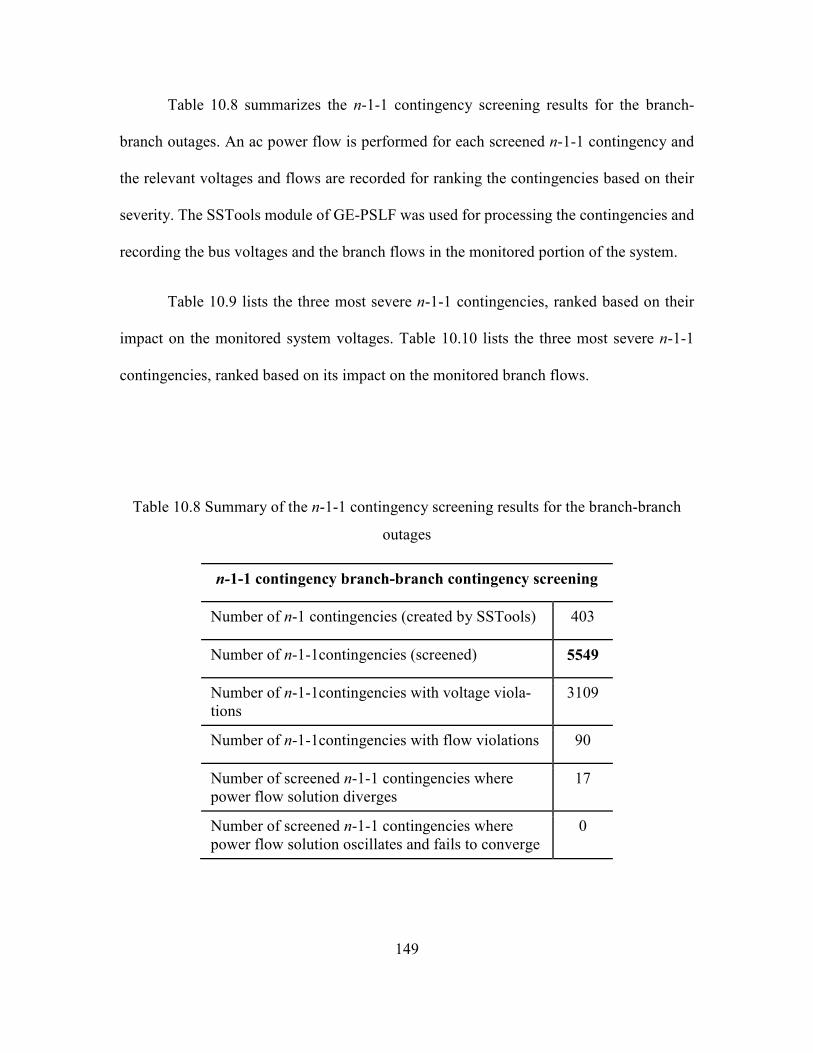
149
Table 10.8 summarizes the n-1-1 contingency screening results for the branch-
branch outages. An ac power flow is performed for each screened n-1-1 contingency and
the relevant voltages and flows are recorded for ranking the contingencies based on their
severity. The SSTools module of GE-PSLF was used for processing the contingencies and
recording the bus voltages and the branch flows in the monitored portion of the system.
Table 10.9 lists the three most severe n-1-1 contingencies, ranked based on their
impact on the monitored system voltages. Table 10.10 lists the three most severe n-1-1
contingencies, ranked based on its impact on the monitored branch flows.
Table 10.8 Summary of the n-1-1 contingency screening results for the branch-branch
outages
n-1-1 contingency branch-branch contingency screening
Number of n-1 contingencies (created by SSTools) 403
Number of n-1-1contingencies (screened) 5549
Number of n-1-1contingencies with voltage viola-
tions
3109
Number of n-1-1contingencies with flow violations 90
Number of screened n-1-1 contingencies where
power flow solution diverges
17
Number of screened n-1-1 contingencies where
power flow solution oscillates and fails to converge
0
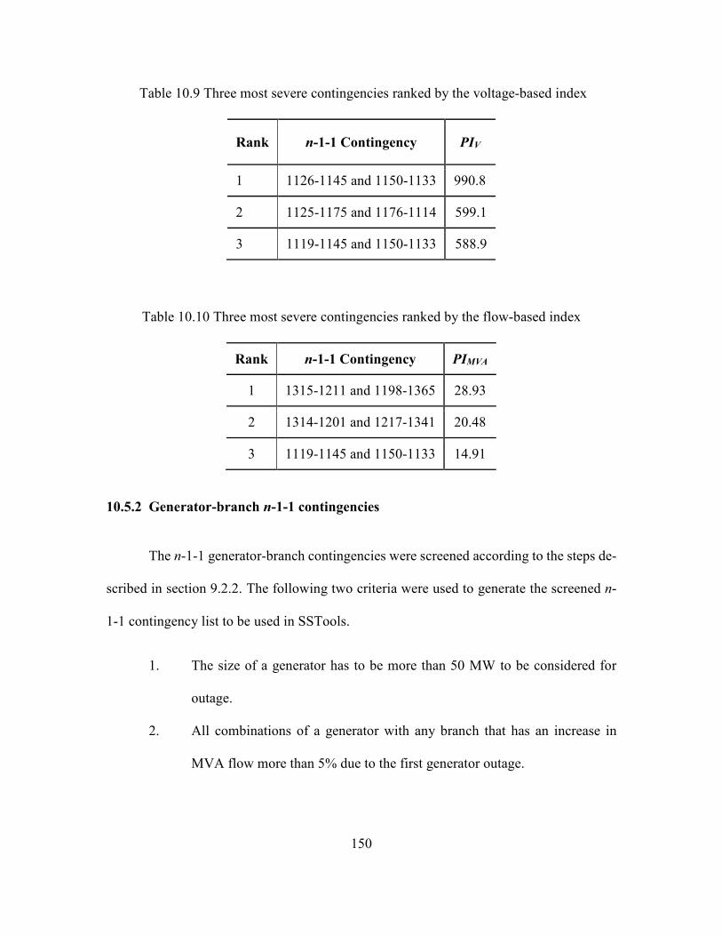
150
Table 10.9 Three most severe contingencies ranked by the voltage-based index
Rank n-1-1 Contingency PIV
1 1126-1145 and 1150-1133 990.8
2 1125-1175 and 1176-1114 599.1
3 1119-1145 and 1150-1133 588.9
Table 10.10 Three most severe contingencies ranked by the flow-based index
Rank n-1-1 Contingency PIMVA
1 1315-1211 and 1198-1365 28.93
2 1314-1201 and 1217-1341 20.48
3 1119-1145 and 1150-1133 14.91
10.5.2 Generator-branch n-1-1 contingencies
The n-1-1 generator-branch contingencies were screened according to the steps de-
scribed in section 9.2.2. The following two criteria were used to generate the screened n-
1-1 contingency list to be used in SSTools.
1. The size of a generator has to be more than 50 MW to be considered for
outage.
2. All combinations of a generator with any branch that has an increase in
MVA flow more than 5% due to the first generator outage.

151
3. All combinations of two generators, which causes the estimated MVA flow
on any branch to exceed 80% of its emergency rating
Table 10.11 summarizes the n-1-1 contingency analysis results for the generator-
branch outages. A re-dispatch based on the generation re-dispatch schedule provided by
the utility is performed after the first generator outage before the second branch outage. An
ac power flow is performed for each screened n-1-1 contingency and the relevant voltages
and flows are recorded. The SSTools module of GE-PSLF was used for processing the
contingencies and recording the bus voltages and the branch flows in the monitored portion
of the system.
From Table 10.11 it can be seen that five cases of n-1-1 generator-branch contin-
gencies were reported to have voltage violations and one case had flow violation. However,
these are the same violations reported during the n-1 branch contingency analysis. No new
violations were observed due to the additional outage. Since no contingency was identified
as critical, the contingency ranking process can be omitted for the n-1-1 generator-branch
contingencies.
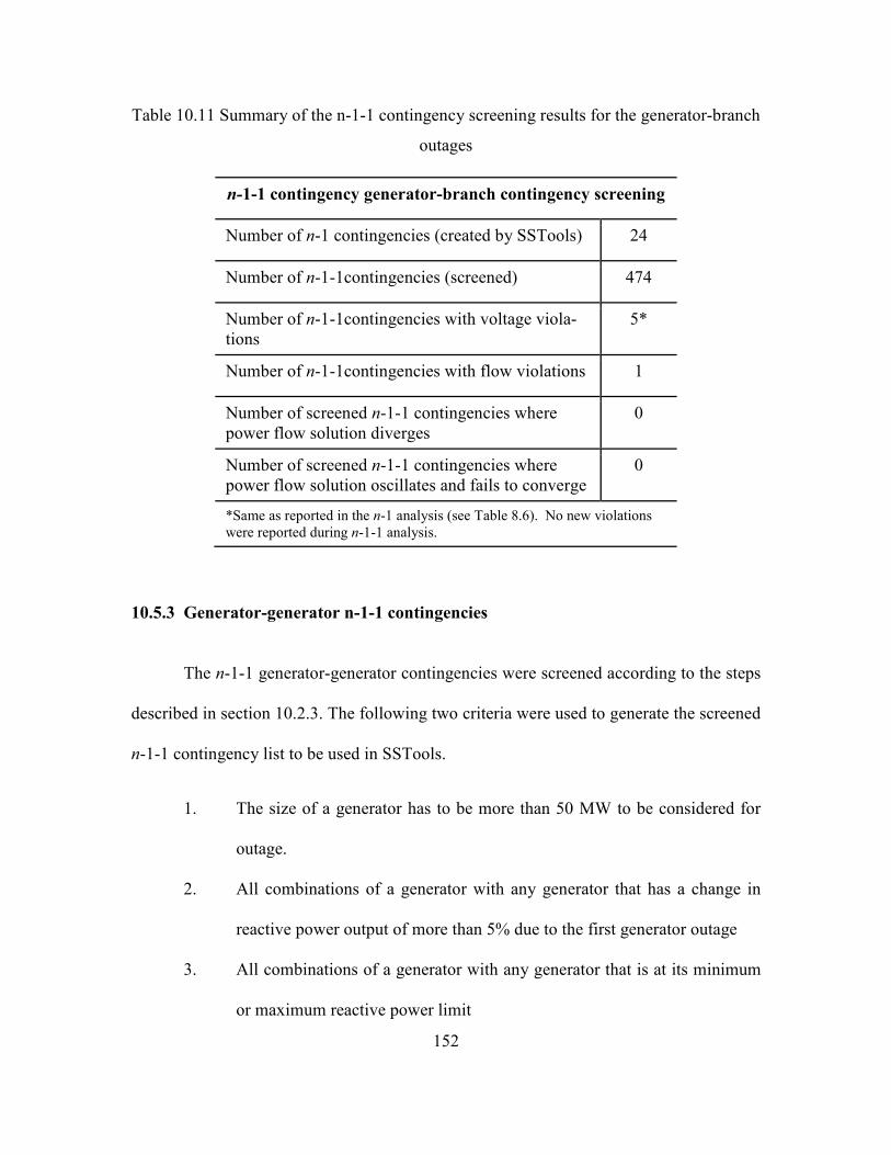
152
Table 10.11 Summary of the n-1-1 contingency screening results for the generator-branch
outages
n-1-1 contingency generator-branch contingency screening
Number of n-1 contingencies (created by SSTools) 24
Number of n-1-1contingencies (screened) 474
Number of n-1-1contingencies with voltage viola-
tions
5*
Number of n-1-1contingencies with flow violations 1
Number of screened n-1-1 contingencies where
power flow solution diverges
0
Number of screened n-1-1 contingencies where
power flow solution oscillates and fails to converge
0
*Same as reported in the n-1 analysis (see Table 8.6). No new violations
were reported during n-1-1 analysis.
10.5.3 Generator-generator n-1-1 contingencies
The n-1-1 generator-generator contingencies were screened according to the steps
described in section 10.2.3. The following two criteria were used to generate the screened
n-1-1 contingency list to be used in SSTools.
1. The size of a generator has to be more than 50 MW to be considered for
outage.
2. All combinations of a generator with any generator that has a change in
reactive power output of more than 5% due to the first generator outage
3. All combinations of a generator with any generator that is at its minimum
or maximum reactive power limit

153
Table 10.12 shows the summary of the n-1-1 contingency analysis results for gen-
erator-generator outages. A re-dispatch based on the generation re-dispatch schedule pro-
vided by the utility is performed after the first generator outage before disconnecting the
second generator. An inertial re-dispatch is performed after the second generator is discon-
nected. An ac power flow is performed for each screened n-1-1 contingency and the rele-
vant voltages and flows are recorded. The SSTools module of GE-PSLF was used for pro-
cessing the contingencies and recording the bus voltages and the branch flows in the mon-
itored portion of the system.
From Table 10.12 it can be seen no voltage or flow violations were reported. Since
no contingency was identified as critical, the contingency ranking process can be omitted
for the n-1-1 generator-generator contingencies.
Table 10.12 Summary of the n-1-1 contingency screening results for the generator-gener-
ator outages
n-1-1 generation contingencies (generator and generator)
Number of n-1-1 contingencies (screened) 249
Number of contingencies causing
voltage violations
over-voltages (> 1.08 pu) 0
under-voltages (< 0.95 pu) 0
Number of contingencies causing flow violations 0
Number of screened n-1-1 contingencies where power flow solu-
tion diverges
0
Number of screened n-1-1 contingencies where power flow solu-
tion oscillates and fails to converge
0

154
10.6 Analysis of contingencies where power flow fails to solve
As discussed earlier, the contingency cases where an ac power flow fails to solve
need to be analyzed further. Since a power flow solution cannot be obtained, the type of
problem caused in the system by these contingencies cannot be determined with certainty.
Therefore, a different approach needs to be undertaken to ascertain the type of problem
that is caused due to these contingencies. Cases where an ac power flow fails to solve are
not very commonly encountered in n-1 contingency analysis. This is evident from the n-
1 contingency analysis results listed in Table 10.5 and Table 10.6. Out of the 403 possible
n-1 contingencies, only 1 case leads to the divergence of the power flow solution. However,
for n-1-1 contingencies, 17 cases were observed where the power flow solution diverges.
This is because n-1-1 contingencies result in the loss of two system components, which is
more severe compared to n-1 outages. These contingencies can be examined by performing
a dynamic study, which simulates the opening of the second line. Such a time domain sim-
ulation can be performed as follows:
1. A power-flow is solved for the first outage. The power-flow solution is
taken as the initial condition for the time domain simulation.
2. A time domain simulation is run and the second branch is opened at time
instant t=1 sec.
As mentioned in section 10.3, in the n-1 contingency analysis results, the power
flow failed to solve due to severely depressed voltages in a load area close to the discon-
nected branch. For the n-1-1 contingency cases, power flows failed to solve either due to
depressed voltages in load areas or due to instability. Two n-1-1 contingencies cases lead

155
to instability, while the 15 remaining contingencies led to undervoltages at different load
areas in the system. Two such representative cases from the n-1-1 contingency analysis
results are discussed here.
Case a (instability): Outage of branches 1608-1701 and 1608-1509
A schematic one-line diagram of the area of interest is shown in Figure 10.1. 1905
MW active power is injected by the generation units at bus 1800. The disconnected
branches 1608-1701 and 1608-1509 are marked with dotted cross. When these two
branches are opened, the power injected at bus 1800 is exported through the path 1800-
1823. The impedance of the path through the branch 1800-1823 is significantly high. The
high impedance of the connecting path combined with the large power injection results in
a low short circuit ratio at the bus 1800. Hence, opening the two lines causes the units
connected at bus 1800 to go unstable. Figure 10.2 shows the relative rotor angles of selected
generators in the region, when the branches are disconnected. From Figure 10.2, it can be
seen that the rotor angles of the units connected at 1800 (CT1, CT2, CT3) units drift away
after the lines are opened. Generators GT1 and GT2 in Figure 10.2 are two large generators
in the concerned utility’s service area. Angle instability was typically observed in the sys-
tem, when the two main power exporting branches close to large generation units were
disconnected.
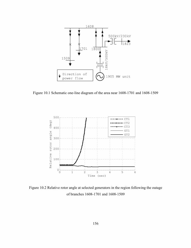
156
Figure 10.1 Schematic one-line diagram of the area near 1608-1701 and 1608-1509
Figure 10.2 Relative rotor angle at selected generators in the region following the outage
of branches 1608-1701 and 1608-1509
0 1 2 3 4 5 60
100
200
300
400
500
Time (sec)
Relative rotor angle (deg)
CT1CT2CT3GT1GT2
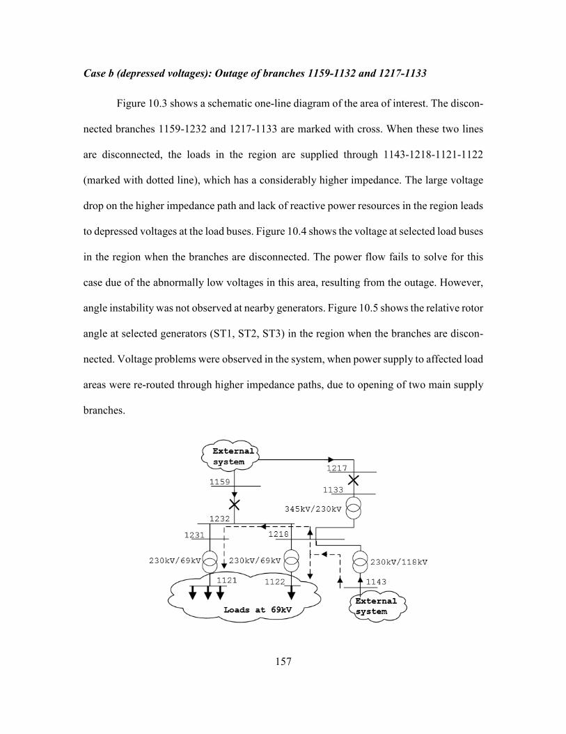
157
Case b (depressed voltages): Outage of branches 1159-1132 and 1217-1133
Figure 10.3 shows a schematic one-line diagram of the area of interest. The discon-
nected branches 1159-1232 and 1217-1133 are marked with cross. When these two lines
are disconnected, the loads in the region are supplied through 1143-1218-1121-1122
(marked with dotted line), which has a considerably higher impedance. The large voltage
drop on the higher impedance path and lack of reactive power resources in the region leads
to depressed voltages at the load buses. Figure 10.4 shows the voltage at selected load buses
in the region when the branches are disconnected. The power flow fails to solve for this
case due of the abnormally low voltages in this area, resulting from the outage. However,
angle instability was not observed at nearby generators. Figure 10.5 shows the relative rotor
angle at selected generators (ST1, ST2, ST3) in the region when the branches are discon-
nected. Voltage problems were observed in the system, when power supply to affected load
areas were re-routed through higher impedance paths, due to opening of two main supply
branches.
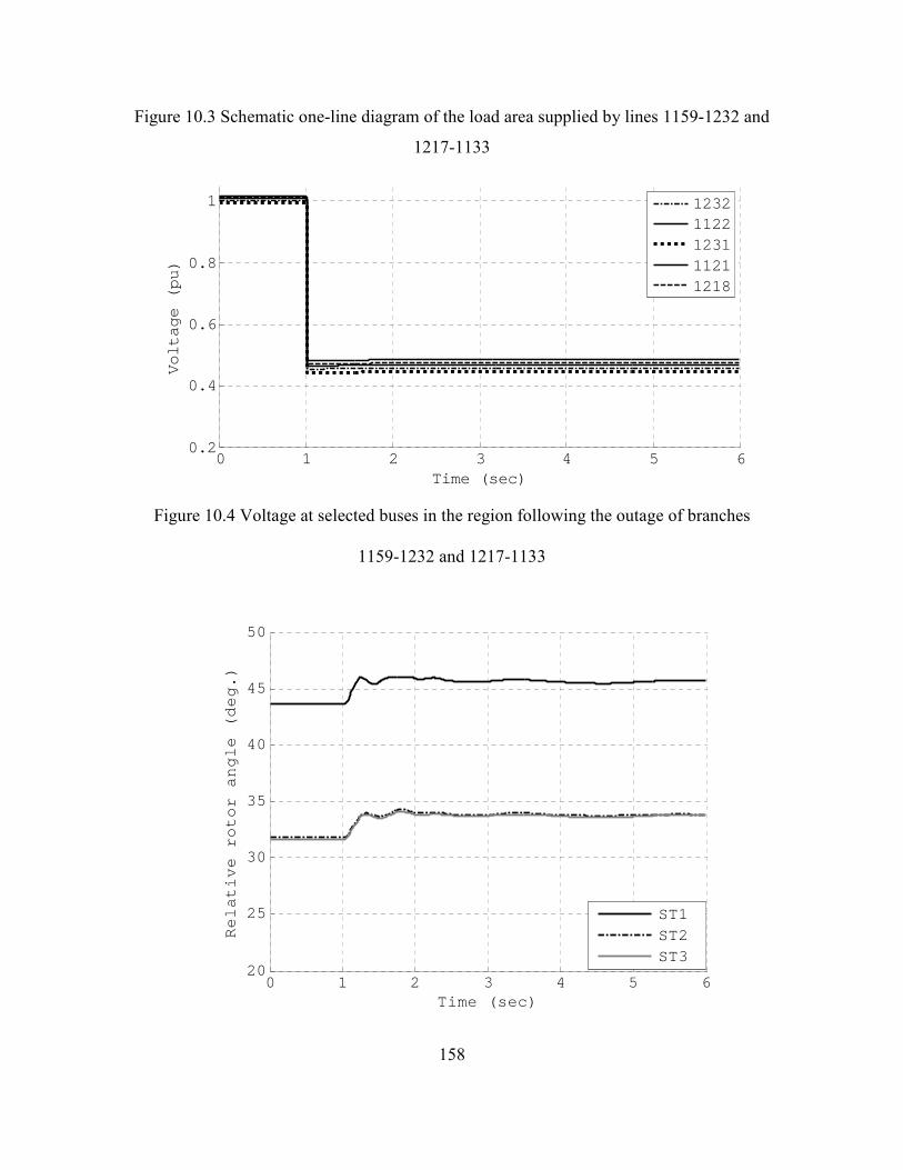
158
Figure 10.3 Schematic one-line diagram of the load area supplied by lines 1159-1232 and
1217-1133
Figure 10.4 Voltage at selected buses in the region following the outage of branches
1159-1232 and 1217-1133
0 1 2 3 4 5 60.2
0.4
0.6
0.8
1
Time (sec)
Voltage (pu)
12321122123111211218
0 1 2 3 4 5 620
25
30
35
40
45
50
Time (sec)
Relative rotor angle (deg.)
ST1ST2ST3
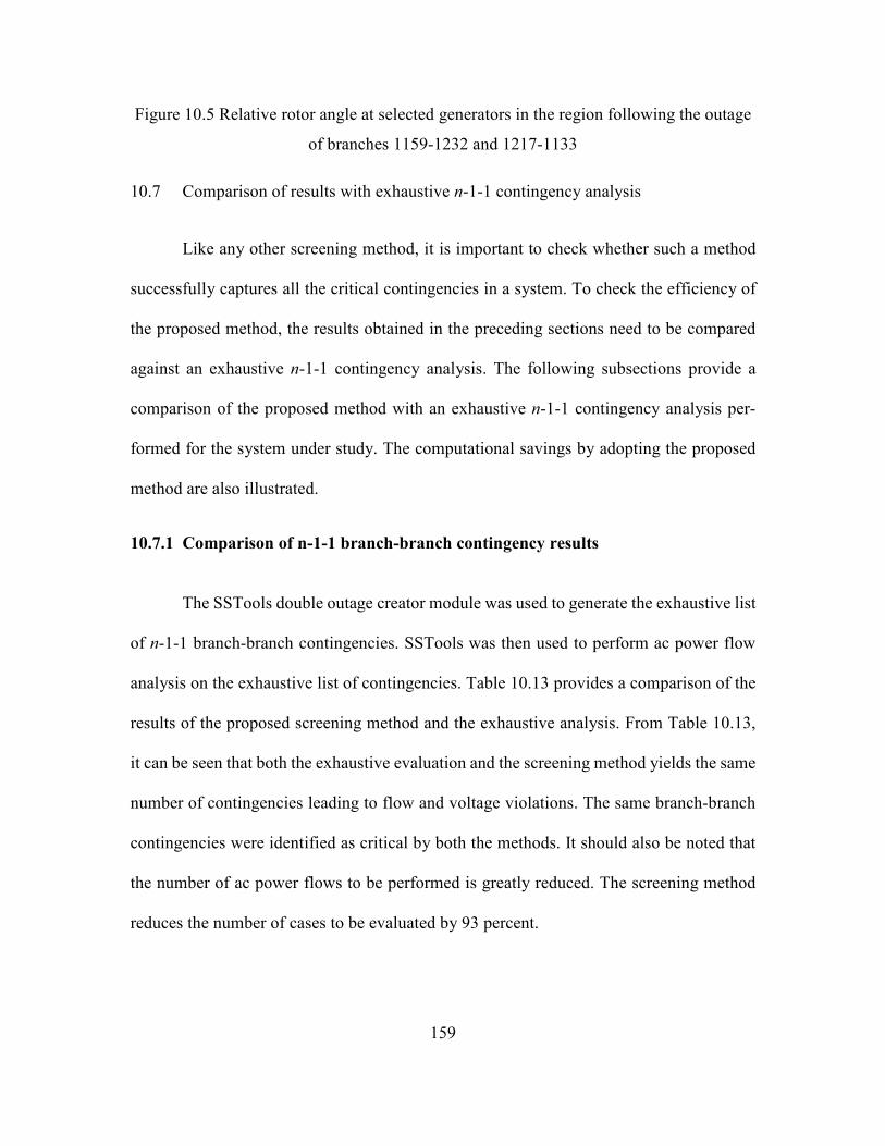
159
Figure 10.5 Relative rotor angle at selected generators in the region following the outage
of branches 1159-1232 and 1217-1133
10.7 Comparison of results with exhaustive n-1-1 contingency analysis
Like any other screening method, it is important to check whether such a method
successfully captures all the critical contingencies in a system. To check the efficiency of
the proposed method, the results obtained in the preceding sections need to be compared
against an exhaustive n-1-1 contingency analysis. The following subsections provide a
comparison of the proposed method with an exhaustive n-1-1 contingency analysis per-
formed for the system under study. The computational savings by adopting the proposed
method are also illustrated.
10.7.1 Comparison of n-1-1 branch-branch contingency results
The SSTools double outage creator module was used to generate the exhaustive list
of n-1-1 branch-branch contingencies. SSTools was then used to perform ac power flow
analysis on the exhaustive list of contingencies. Table 10.13 provides a comparison of the
results of the proposed screening method and the exhaustive analysis. From Table 10.13,
it can be seen that both the exhaustive evaluation and the screening method yields the same
number of contingencies leading to flow and voltage violations. The same branch-branch
contingencies were identified as critical by both the methods. It should also be noted that
the number of ac power flows to be performed is greatly reduced. The screening method
reduces the number of cases to be evaluated by 93 percent.
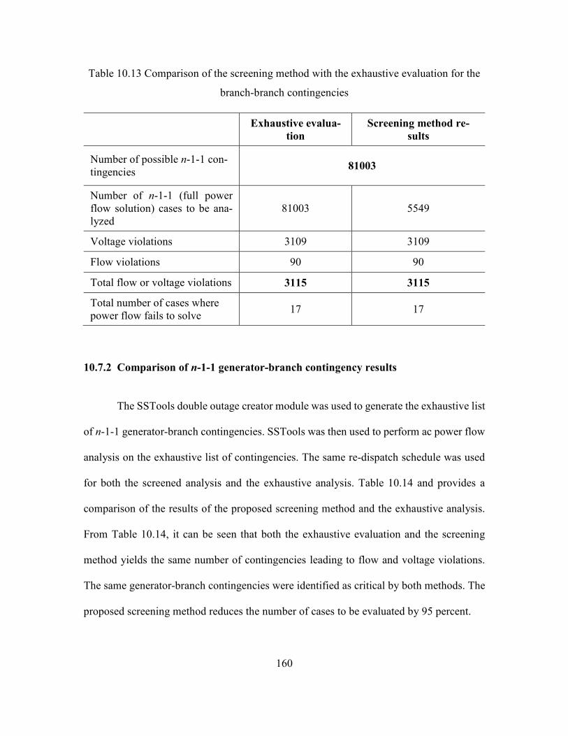
160
Table 10.13 Comparison of the screening method with the exhaustive evaluation for the
branch-branch contingencies
Exhaustive evalua-
tion
Screening method re-
sults
Number of possible n-1-1 con-
tingencies 81003
Number of n-1-1 (full power
flow solution) cases to be ana-
lyzed
81003 5549
Voltage violations 3109 3109
Flow violations 90 90
Total flow or voltage violations 3115 3115
Total number of cases where
power flow fails to solve 17 17
10.7.2 Comparison of n-1-1 generator-branch contingency results
The SSTools double outage creator module was used to generate the exhaustive list
of n-1-1 generator-branch contingencies. SSTools was then used to perform ac power flow
analysis on the exhaustive list of contingencies. The same re-dispatch schedule was used
for both the screened analysis and the exhaustive analysis. Table 10.14 and provides a
comparison of the results of the proposed screening method and the exhaustive analysis.
From Table 10.14, it can be seen that both the exhaustive evaluation and the screening
method yields the same number of contingencies leading to flow and voltage violations.
The same generator-branch contingencies were identified as critical by both methods. The
proposed screening method reduces the number of cases to be evaluated by 95 percent.
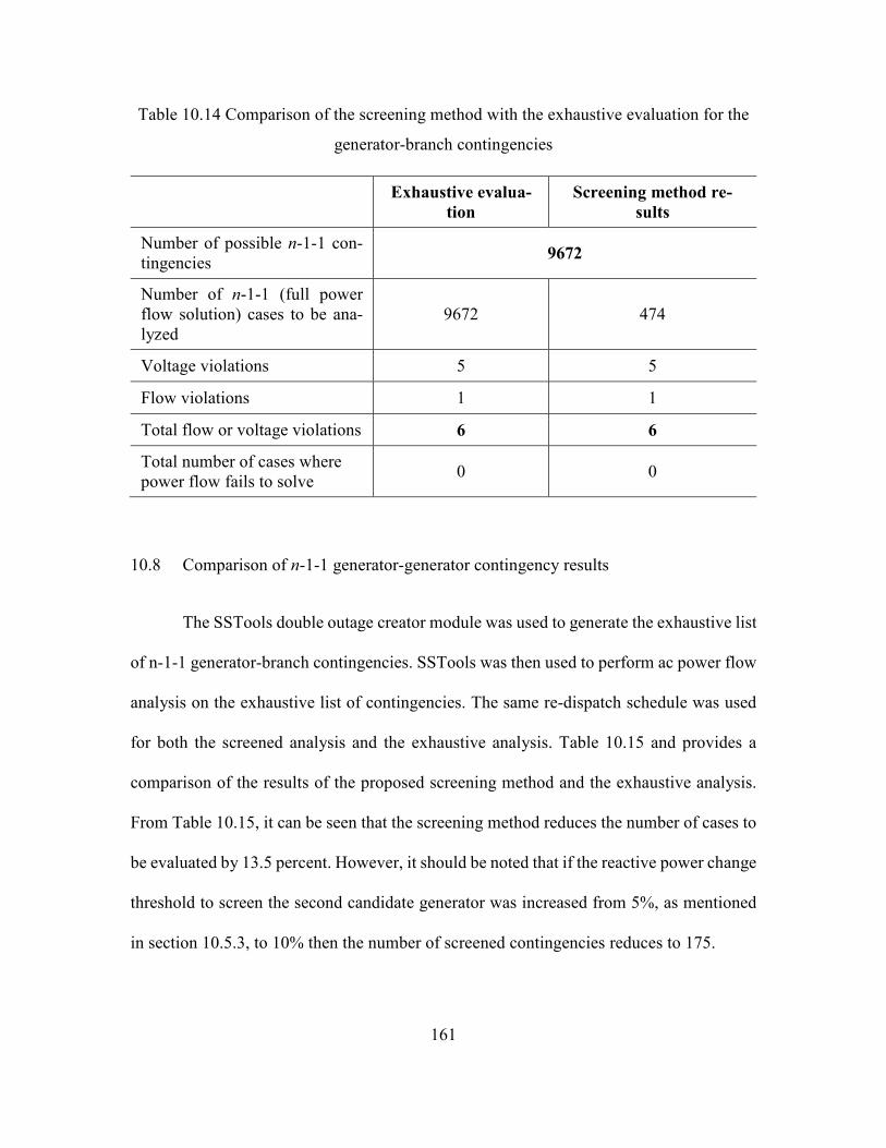
161
Table 10.14 Comparison of the screening method with the exhaustive evaluation for the
generator-branch contingencies
Exhaustive evalua-
tion
Screening method re-
sults
Number of possible n-1-1 con-
tingencies 9672
Number of n-1-1 (full power
flow solution) cases to be ana-
lyzed
9672 474
Voltage violations 5 5
Flow violations 1 1
Total flow or voltage violations 6 6
Total number of cases where
power flow fails to solve 0 0
10.8 Comparison of n-1-1 generator-generator contingency results
The SSTools double outage creator module was used to generate the exhaustive list
of n-1-1 generator-branch contingencies. SSTools was then used to perform ac power flow
analysis on the exhaustive list of contingencies. The same re-dispatch schedule was used
for both the screened analysis and the exhaustive analysis. Table 10.15 and provides a
comparison of the results of the proposed screening method and the exhaustive analysis.
From Table 10.15, it can be seen that the screening method reduces the number of cases to
be evaluated by 13.5 percent. However, it should be noted that if the reactive power change
threshold to screen the second candidate generator was increased from 5%, as mentioned
in section 10.5.3, to 10% then the number of screened contingencies reduces to 175.
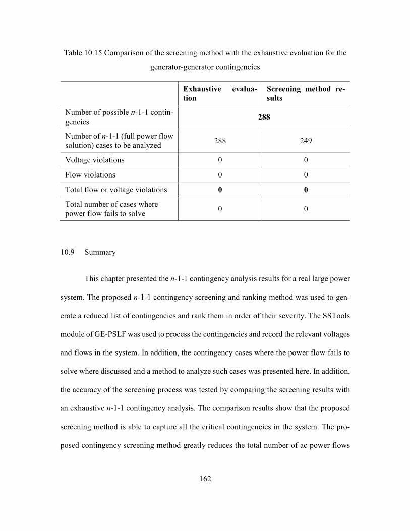
162
Table 10.15 Comparison of the screening method with the exhaustive evaluation for the
generator-generator contingencies
Exhaustive evalua-
tion
Screening method re-
sults
Number of possible n-1-1 contin-
gencies 288
Number of n-1-1 (full power flow
solution) cases to be analyzed 288 249
Voltage violations 0 0
Flow violations 0 0
Total flow or voltage violations 0 0
Total number of cases where
power flow fails to solve 0 0
10.9 Summary
This chapter presented the n-1-1 contingency analysis results for a real large power
system. The proposed n-1-1 contingency screening and ranking method was used to gen-
erate a reduced list of contingencies and rank them in order of their severity. The SSTools
module of GE-PSLF was used to process the contingencies and record the relevant voltages
and flows in the system. In addition, the contingency cases where the power flow fails to
solve where discussed and a method to analyze such cases was presented here. In addition,
the accuracy of the screening process was tested by comparing the screening results with
an exhaustive n-1-1 contingency analysis. The comparison results show that the proposed
screening method is able to capture all the critical contingencies in the system. The pro-
posed contingency screening method greatly reduces the total number of ac power flows

163
that need to be performed. Therefore, the proposed technique enables significant savings
in computational effort.
164
CHAPTER 11: PROPOSED N-1-1 CONTINGENCY SCREENING AND CLASSIFI-
CATION FOR DSA
DSA for n-1-1 contingencies examines whether a system is able to maintain stabil-
ity following a sequential outage of two network elements. The contingency events referred
to in this chapter are three-phase faults on lines followed by removal of the faulted lines
from service by appropriate protection devices. Faults are large disturbances on the system
and have a significant impact on the transient stability.
11.1 Contingency screening and classification for DSA
DSA for n-1-1 contingencies is done in two steps. The first step is to simulate the
initial contingency and check whether it is stable. If the system is stable and reaches an
acceptable equilibrium after all automatic controls have acted, the second contingency is
simulated. If the second contingency is stable and an acceptable steady state is reached, the
n-1-1 contingency is labeled as secure. Otherwise, the n-1-1 contingency is labeled as in-
secure. n-1-1 contingency screening and classification for DSA will be simply referred to
as n-1-1 contingency screening and classification for the remainder of the report.
As discussed earlier, one of the main challenges for n-1-1 contingency screening
and classification is the large number of cases that need to be evaluated. As such, perform-
ing simplified fast calculations can become computationally prohibitive for realistic power
systems. This part of the report focuses on the development of a fast and reliable method
for screening and classifying n-1-1 contingencies. A two-stage approach is used to screen
and classify the n-1-1 contingencies. In stage I, a subset of n-1-1 contingencies is screened
for further classification. The screening process is based on the power flow results of the
165
n-1 analysis. In stage II, the screened contingencies are classified based on the kinetic en-
ergy gained due to the fault and the change in the magnitude of the Thévenin's impedance
(Zth) at the point of interconnection (POI) of the generators in the post-fault network. The
proposed screening and classification method is implemented using MATLAB and GE-
PSLF. The following sections provide detailed descriptions of stage I and stage II of the
proposed method followed by a justification of the processes.
11.1.1 Stage I: Screening of n-1-1 contingencies
Stage I of the n-1-1 contingency screening and classification process deals with
screening a subset of all possible n-1-1 contingencies, for further analysis. The screening
process is based on the power flow results of the n-1 contingency analysis. The power flow
solution after a contingency describes the post-disturbance equilibrium of the system, once
all fast control actions have taken place. The impact of the second contingency on the sys-
tem is dependent on this equilibrium point and hence the n-1 power flow solution is the
starting point for the n-1-1 screening process. It should be noted that only stable n-1 con-
tingencies are considered as the first contingencies in the screening process for n-1-1 anal-
ysis. This is a valid consideration as it is meaningless to analyze a successive contingency
if the initial contingency is not stable. To generate the list of the screened n-1-1 contingen-
cies involving branch-branch outages, the following steps are followed [87]:
1. Perform a full ac power-flow for all n-1 branch contingencies and record all
the line MW flows.
2. For each branch outage, compute the percentages of MW flow in the outage
branch that shows up in all other branches in the system. This percentage is

166
the similar to the line outage distribution factor (LODF) and will be referred
to as MWLODF in the rest of this report. As an example, the MWLODF in
a hypothetical line A for outage of line B is computed as follows:
100,
,,1
−= −
Bbase
AbaseABn
ABMW
MWMWMWLODF , (11.1)
where,
MWLODFAB is the percentage of MW flow on line B that shows up on line
A.
MWn-1,AB is the MW flow on line A with line B disconnected.
MWbase,A is the MW flow on line A in the base case ( all lines in service).
MWbase,B is the MW flow on line B in the base case ( all lines in service).
3. All branches that have an MWLODF more than a set threshold for an n-1
contingency are screened as candidate branches for the second outage fol-
lowing that particular n-1 contingency.
4. The n-1-1 contingency list is updated to include all pairs of the n-1 outages
and the corresponding screened second outages in step 3. Steps 2 to 4 are
performed for all n-1 contingencies.
5. Finally, all duplicate n-1-1 contingencies are removed from the list and the
pre-screened list of n-1-1 contingency I formed.
The screening method described here is similar to the screening method described
in section 9.2.1 with the exception of using the MWLODF instead of the ACLODF. The
screening process uses the change in MW flow as a screening parameter to select candidate
branches for the second outage. Since dynamic security is of concern, change in the MW

167
flow is a suitable screening parameter as it influences the rotor angles of the generators in
a system. A higher value of MWLODF indicates that the system has a radial structure in
the region of interest and only a few branches compensate for the lost flow on the discon-
nected branch. This implies that the branch may be closer to a generation source or a load
center where the network is close to radial. A fault on a line with a high MWLODF can be
critical as the disturbance may be close to a generator or group of generators. Subsequent
disconnection of the line to clear the fault can result in a weak post-disturbance network
due to loss of a main transmission path. A lower value of the MWLODF indicates that the
network is meshed and only a small fraction of the lost flow on the disconnected line shows
up in the other lines. Power systems are typically meshed farther away from generation
sources and load centers. Faults at such locations followed by the removal of the affected
line neither causes a large disturbance nor weakens the transmission system significantly.
It is worthwhile to mention that a higher value of the MWLODF does imply that a fault on
the corresponding line will be more severe than on others. However, it is a good measure
to identify critical lines, where faults could be possibly severe. The MWLODF serves as an
index to screen critical lines rather than a measure of severity.
The screening process is conservative in the sense that not all screened cases are
unstable. It should be noted that stability assessment is not an issue here. The screening
and classification process aims to prioritize the analysis of cases, which are critical from a
stability assessment viewpoint. The n-1-1 contingencies eliminated by the screening pro-
cess are categorized as of least concern (LCR) for stability assessment. The screening pro-
cess is expected to reduce the number of cases significantly, that need to be analyzed in
stage II.

168
11.1.2 Stage II: Classification of screened n-1-1 contingencies
Stage II deals with classifying the screened n-1-1 contingencies obtained from stage
I. The screened contingencies are classified based on two factors:
1. The total kinetic energy gained by the machines due to the applied fault
2. The maximum change in the magnitude of Zth seen at the POI of a generator
or a group of generators due to the removal of the faulted line from service
A short time domain simulation is conducted to compute the kinetic energy gained
by the system at the end of the fault. Additionally, the change in the magnitude of Zth as
seen at the POIs of all generators/group of generators in the area of interest is computed
after opening the faulted line. It is assumed that a fault applied on the system will be cleared
in 5 cycles, which is a standard clearing time for modern circuit breakers rated for 100kV
and above [90]. Based on the two measurements the contingencies are categorized as crit-
ical (CR), possibly critical (PCR) and non-critical (NCR). The following steps are followed
to classify the screened contingencies:
1. Solve the power flow by removing the first line considered in n-1 contin-
gency.
2. Perform a time domain simulation and apply a 5-cycle three-phase fault on
the screened second line considered in the n-1-1 case. The time domain sim-
ulation is run only the till the fault is cleared.
3. Record the angular speed of selected generators at the end of the fault and
compute the total kinetic energy gained by the system with respect to the

169
center of inertia (COI) [78] of the area of interest. The total kinetic energy
gained during the fault is given by:
∑
∑=
gens all
gens all
i
ii
coiM
M ωω (11.2)
coiii ωωω −=∆ (11.3)
2
gens all 2
1)(JKE ii ω∆∑= (11.4)
where,
ωcoi is the angular velocity of the center of inertia
ωi is the angular velocity of the ith generator
Mi is the inertia constant of the ith generator
KE is the kinetic energy gained by the system
Ji is the moment of inertia of the ith generator
4. Remove the faulted line from service and compute the change in the mag-
nitude of Zth as seen at the POIs of all generators/group of generators in the
region of interest.
5. Record the maximum change in the magnitude of Zth and the corresponding
bus number of the POI where it occurs. The maximum change in the mag-
nitude of Zth will be referred to as |∆Zthmax| in the rest of the report.
The stability of a power system during a fault depends on the kinetic energy gained
by the system due to the fault and the robustness of the post-disturbance network [91]. This

170
can be understood by examining the equal area criterion for a one-machine infinite bus
system. The idea has been extended to multi-machine systems as well [92]. During a fault,
the ability of the network to export electrical power is severely restricted causing the ma-
chine to accelerate. Once the fault is cleared by opening the faulted line, the machine is
able to export electrical power and it decelerates. The stability of the machine is dependent
on its ability to decelerate in the post-disturbance condition and reach a steady state.
The kinetic energy gained by the system during a fault is computed by performing
a short time domain simulation with a three-phase fault applied on the concerned branch.
To estimate the ability of the system to decelerate, the change in the magnitude of Zth seen
into the system at the POI of the generator due to opening of the faulted line is computed.
The buses, which are the POI of generating stations, are typically known to planners be-
forehand. The change in Zth can be computed by using sparsity oriented compensation
methods [93]. A review of the swing equation [91] indicates that a large change in the
magnitude of Zth results in a substantial reduction in the peak of the post-fault swing curve
as compared to the pre-faulted condition. A reduction in the peak of the post-fault swing
curve limits the ability of the generator to decelerate, thereby making it prone to instability.
Hence, these two factors are chosen to categorize contingencies based on their impact on
stability.
11.2 Categorization of n-1-1 contingencies
As mentioned in section 11.1.2, the screened contingencies are further grouped into
three distinct categories. The three categories are CR, PCR, and NCR. Based on the kinetic

171
energy gained and the |∆Zthmax|, each contingency is assigned one of these categories. Brief
descriptions of the three different categories are as follows:
I. Critical (CR)
A Contingency is categorized as CR if both the kinetic energy and the |∆Zthmax|
due to the contingency are high. A critical contingency implies that the fault is
close to a generator and opening of the faulted line weakens the transmission
system. Such cases are likely to have stability issues and warrant detailed time
domain analysis
II. Possibly critical (PCR)
A Contingency that results in large kinetic energy and small |∆Zthmax| or small
kinetic energy and large |∆Zthmax| is categorized as PCR. A large kinetic energy
and small |∆Zthmax| implies that although the fault is close to generation units,
the post disturbance network is strong. On the other hand, a large |∆Zthmax| and
small kinetic energy indicates that although the post-fault network is weak, the
fault is electrically distant from large generation units. Contingencies catego-
rized as PCR may not be unstable under a given operating condition, but can
become critical as the operating conditions change.
III. Non critical (NCR)
Contingencies that result in both small kinetic energy and small |∆Zthmax| are
categorized as NCR. Detailed time domain analysis is not required for these
contingencies.
Once the contingencies are categorized as CR, PCR and NCR, they can be dis-
played on a kinetic energy vs. |∆Zthmax| plot for ease of visualization. The visualization
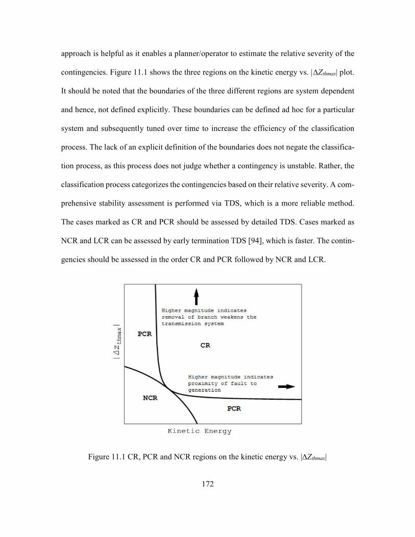
172
approach is helpful as it enables a planner/operator to estimate the relative severity of the
contingencies. Figure 11.1 shows the three regions on the kinetic energy vs. |∆Zthmax| plot.
It should be noted that the boundaries of the three different regions are system dependent
and hence, not defined explicitly. These boundaries can be defined ad hoc for a particular
system and subsequently tuned over time to increase the efficiency of the classification
process. The lack of an explicit definition of the boundaries does not negate the classifica-
tion process, as this process does not judge whether a contingency is unstable. Rather, the
classification process categorizes the contingencies based on their relative severity. A com-
prehensive stability assessment is performed via TDS, which is a more reliable method.
The cases marked as CR and PCR should be assessed by detailed TDS. Cases marked as
NCR and LCR can be assessed by early termination TDS [94], which is faster. The contin-
gencies should be assessed in the order CR and PCR followed by NCR and LCR.
Figure 11.1 CR, PCR and NCR regions on the kinetic energy vs. |∆Zthmax|
173
11.3 Summary
This chapter presented the proposed n-1-1 contingency screening and classification
method for DSA. The proposed method works in two stages. In stage I, candidate n-1-1
contingencies are screened for the contingency classification process. In stage II, the
screened n-1-1 contingencies from stage I are classified into four distinct groups CR, PCR,
NCR and LCR. The contingencies categorized as CR and PCR are important from a tran-
sient stability viewpoint and warrant detailed analysis. The contingencies categorized as
NCR and LCR are of the lowest priority for stability analysis. These contingencies do not
need any detailed evaluation. Furthermore, a visualization approach is suggested which
enables a better presentation of the contingency classification results. The proposed screen-
ing and classification method is expected to reduce the computational effort by reducing
the number of cases that needs detailed evaluation.

174
CHAPTER 12: N-1-1 CONTINGENCY ANALYSIS FOR DSA: APPLICATION TO A
REAL SYSTEM
In chapter 11, a method for screening and classifying n-1-1 contingencies was pro-
posed. In this chapter, the proposed method is used to screen and classify n-1-1 contingen-
cies for the selected utility in the WECC system. For DSA, the contingencies are screened
and classified with respect to their impact on the system stability. In the following sections,
the various thresholds used for the contingency screening process are presented. In addi-
tion, some examples are provided which highlight the main features of the proposed
method.
12.1 Description of the case
Contingency screening and classification was performed for the same utility con-
sidered in chapter 10. In addition to using the power flow file, the dynamic data file con-
taining the equipment dynamic models was used in this part of the work. The description
of the WECC system and the selected utility’s service area can be found in Table 10.1.
12.2 n-1 contingency screening and classification for the selected utility
Due to the lesser number of n-1 contingencies, the screening process of stage I can
be omitted and the contingencies can be directly classified using the classification tech-
nique. Since the screening process is skipped, the list LCR for n-1 contingencies has no
entries in it. Based on the dynamic characteristics, the contingencies are classified into
three groups, CR, PCR and NCR. For the classification process, a 5-cycle three-phase fault
175
is considered as the disturbance on the system. It is assumed that the protection system
clears the fault by removing the faulted line from service within 5-cycles [90].
MATLAB and GE-PSLF, was used to perform the n-1 contingency classification.
The SSTools module of GE-PSLF was used to generate the n-1 contingency list. The GE-
PSLF transient stability module [22] was used to perform the time domain simulations.
MATLAB was used to analyze the output from PSLF and perform the remainder of the
computations.
For the n-1 contingency classification study, the results are presented directly with-
out detailed discussions. A comprehensive analysis of the method and results are presented
later in the section dealing with n-1-1 contingency screening and classification. The n-1-1
contingencies provide a better insight into the screening and classification process and
hence the detailed analysis is left for later. The following subsection presents the results of
the n-1 contingency classification process.
12.2.1 n-1 contingency analysis results
SSTools generated a list of 403 branch-branch contingencies for the area/zones and
voltage levels described in section 10.1. The contingencies were then classified as CR,
PCR, and NCR as described in the section 11.2. 13 n-1 contingencies resulted in islanding
of generation units. Islanding of generation units was detected by a large change in the
|∆Zthmax| at the POI of these generation units. These 13 n-1 contingencies are excluded from
further analysis. Figure 12.1 shows the location of the contingencies on a kinetic energy vs
|∆Zthmax| plot. Contingencies that lead to islanding of generation units are not shown in
Figure 12.1. The three different categories of contingencies are marked distinctly on the

176
plot. From Figure 12.1, it can be seen that none of the n-1 contingencies fall in the category
CR. Detailed TDSs were performed for all the contingencies in the category PCR. All these
contingencies were found to be stable.
Figure 12.1 n-1 contingencies on a kinetic energy vs. |∆Zthmax| plot
12.3 n-1-1 contingency screening and classification for the selected utility
In n-1-1 contingency screening and classification, only stable n-1 contingencies are
considered as first outages. The n-1 contingencies that are unstable or cause islanding of
generation units are listed separately. In this particular study, for the system under consid-
eration, all n-1 contingencies were stable and 13 n-1 contingencies lead to islanding of
generation units. These 13 n-1 contingencies were excluded from the n-1-1 analysis.
The screening process described in stage I of the proposed method was used to
screen candidate lines for simulating the second outage. The MWLODF threshold for
screening candidate lines for the second outage was set to 40%. Lowering the MWLODF
threshold did not result in screening of any additional unstable contingency. Hence, the set

177
threshold is sufficient for the screening process. As mentioned before, the MWLODF can
be tuned over time for more efficient screening of contingencies. After the second set of
candidate lines are screened, a list of the n-1-1 contingencies is created. The screened n-1-
1 contingencies are then classified appropriately by the classification process described in
section 11.2.
12.3.1 n-1-1 contingency analysis results
Table 12.1 lists the number of all possible n-1-1 contingencies and the number of
screened contingencies. The screening process substantially reduces the number of cases
to be classified. As indicated earlier, the screening process of stage I is conservative in
nature. Not all screened contingencies are likely to have dynamic issues. However, the
screening process eliminates all the n-1-1 contingencies that are least critical from a tran-
sient stability perspective [87].
Figure 12.2 shows the location of the screened n-1-1 contingencies on the kinetic
energy vs. |∆Zthmax| plot. The different categories of contingencies are marked distinctly on
the plot. Table 10.2 lists the number of n-1-1 contingencies in the four different categories.
TDS were performed for the 204 screened n-1-1 contingencies. All the contingencies in
the categories PCR and NCR were found to be stable. The 3 contingencies categorized as
CR were found to cause instability. Table 12.3 presents the results of TDS for 8 selected
contingencies in categories CR and PCR. The 8 selected contingencies (otg1-otg8) are
marked in Figure 12.2. The 8 contingencies were chosen the cover the CR cases and the
PCR cases, which resulted in high kinetic energy or high |∆Zthmax|. The contingencies in
the PCR region are stable at this operating condition. This is because in these cases either

178
the fault is far from large generation or the post-disturbance network is strong enough to
provide adequate deceleration to the accelerating generators. Detailed TDS results for otg2,
otg5 and otg7 are presented in Figure 12.3, Figure 12.4, and Figure 12.5 respectively. The
relative rotor angles of the most affected generators due these contingencies are plotted.
Generators G1to G7 are the generators, which are most affected by these contingencies.
From Figure 12.3, it can be seen that contingency otg2, which is grouped as CR leads to
instability. Contingencies otg5 and otg7, which are grouped as PCR, are stable.
Table 12.1 Metrics for the screening process in stage I
Total number of n-1
contingencies
Total number of possible n-1-1
contingencies
Number of n-1-1 screened as
candidate cases
390 75855 204
Figure 12.2 n-1-1 contingencies on a kinetic energy vs. |∆Zthmax|
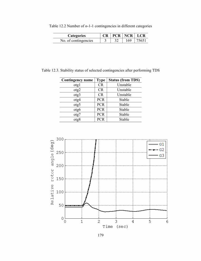
179
Table 12.2 Number of n-1-1 contingencies in different categories
Categories CR PCR NCR LCR
No. of contingencies 3 32 169 75651
Table 12.3. Stability status of selected contingencies after performing TDS
Contingency name Type Status (from TDS)
otg1 CR Unstable
otg2 CR Unstable
otg3 CR Unstable
otg4 PCR Stable
otg5 PCR Stable
otg6 PCR Stable
otg7 PCR Stable
otg8 PCR Stable
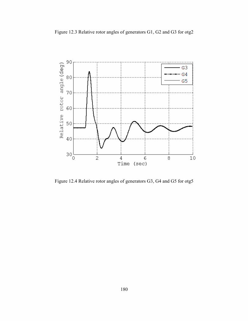
180
Figure 12.3 Relative rotor angles of generators G1, G2 and G3 for otg2
Figure 12.4 Relative rotor angles of generators G3, G4 and G5 for otg5

181
Figure 12.5 Relative rotor angles of generators G3, G6 and G7 for otg7
It is worthwhile to examine the contingencies categorized as PCR in further detail.
As mentioned earlier, these contingencies could become critical due change in operating
conditions. An example to illustrate such a case is as follows:
Case: otg8 - outage of the lines 1518–1519 and 1211-1212
Outage of line 1518–1519 is considered as the n-1 outage. A 5-cycle three-phase
fault on line 1211-1212 and the ensuing outage is considered as the n-1-1 event. Figure
10.6 shows a schematic one-line diagram of the area of interest. From Figure 12.2, it can
be seen that the contingency otg8 results in a large |∆Zthmax|, though the kinetic energy
gained is comparatively less. |∆Zthmax| for this contingency was recorded at bus 1212, which
is the POI of 12 generators CTG1 to CTG 12, each rated at 44 MW. In the present scenario,
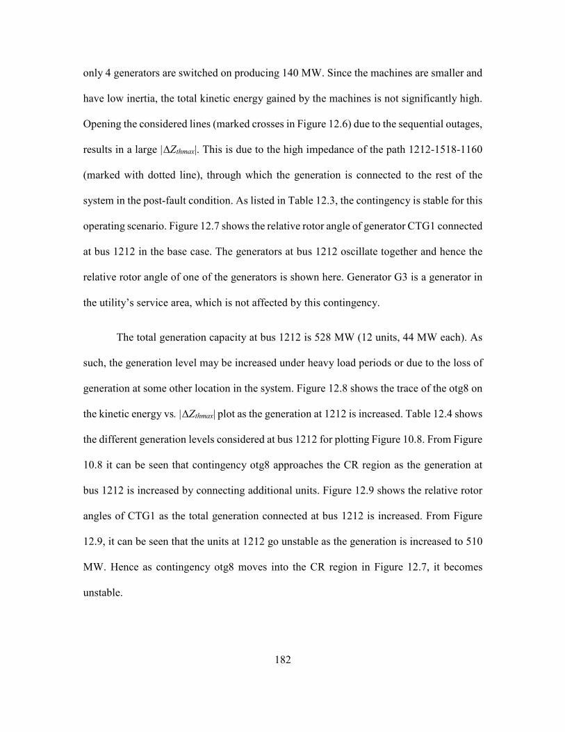
182
only 4 generators are switched on producing 140 MW. Since the machines are smaller and
have low inertia, the total kinetic energy gained by the machines is not significantly high.
Opening the considered lines (marked crosses in Figure 12.6) due to the sequential outages,
results in a large |∆Zthmax|. This is due to the high impedance of the path 1212-1518-1160
(marked with dotted line), through which the generation is connected to the rest of the
system in the post-fault condition. As listed in Table 12.3, the contingency is stable for this
operating scenario. Figure 12.7 shows the relative rotor angle of generator CTG1 connected
at bus 1212 in the base case. The generators at bus 1212 oscillate together and hence the
relative rotor angle of one of the generators is shown here. Generator G3 is a generator in
the utility’s service area, which is not affected by this contingency.
The total generation capacity at bus 1212 is 528 MW (12 units, 44 MW each). As
such, the generation level may be increased under heavy load periods or due to the loss of
generation at some other location in the system. Figure 12.8 shows the trace of the otg8 on
the kinetic energy vs. |∆Zthmax| plot as the generation at 1212 is increased. Table 12.4 shows
the different generation levels considered at bus 1212 for plotting Figure 10.8. From Figure
10.8 it can be seen that contingency otg8 approaches the CR region as the generation at
bus 1212 is increased by connecting additional units. Figure 12.9 shows the relative rotor
angles of CTG1 as the total generation connected at bus 1212 is increased. From Figure
12.9, it can be seen that the units at 1212 go unstable as the generation is increased to 510
MW. Hence as contingency otg8 moves into the CR region in Figure 12.7, it becomes
unstable.
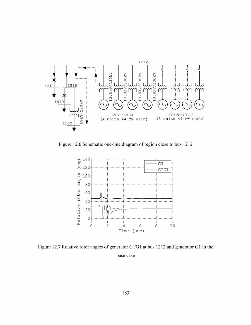
183
Figure 12.6 Schematic one-line diagram of region close to bus 1212
Figure 12.7 Relative rotor angles of generator CTG1 at bus 1212 and generator G1 in the
base case
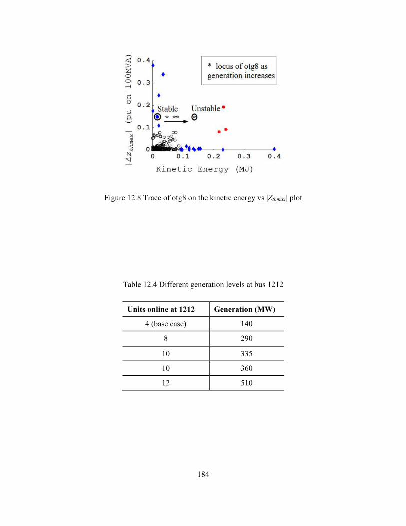
184
Figure 12.8 Trace of otg8 on the kinetic energy vs |Zthmax| plot
Table 12.4 Different generation levels at bus 1212
Units online at 1212 Generation (MW)
4 (base case) 140
8 290
10 335
10 360
12 510
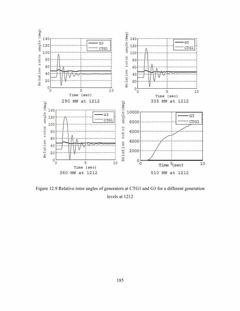
185
Figure 12.9 Relative rotor angles of generators at CTG1 and G3 for a different generation
levels at 1212
186
12.4 Summary
This chapter presented the n-1-1 contingency screening and classification results
for the selected utility in the WECC area. The contingency screening and classification
method is applicable for branch-branch contingencies, which have significant impact on
transient stability. The proposed method is used to generate a reduced list of n-1-1 contin-
gencies and classify them based on their dynamic behavior. The screened contingencies
are classified into four distinct groups CR, PCR, NCR and LCR based on their impact on
the system. Furthermore, examples were provided to illustrate the different aspects of the
screening and classification process. The important feature of the proposed method is that
it reduces the computational burden significantly. The screening process reduces the num-
ber of contingencies that needs to be classified substantially. Further, the classification
process identifies the cases that need detailed evaluation, without the need of any elaborate
computation.
187
CHAPTER 13: CONCLUSIONS AND FUTURE WORK: N-1-1 CONTINGENCY
ANALYSIS
13.1 Conclusions
Power system security assessment for n-1-1 contingencies is of paramount im-
portance for the secure and reliable operation of power systems. The primary impediment
in performing such assessments is the overwhelming number of cases that need to be ana-
lyzed. The work done here presents a systematic approach to n-1-1 power system security
assessment for a realistic large power system. An n-1-1 contingency screening and ranking
method was proposed for SSA and an n-1-1 contingency screening and classification
method was proposed for DSA. The key merit of the proposed methods lies in the simplic-
ity of their implementation and reliability in identifying the critical contingencies. The
main conclusions of the study are as follows:
1. The proposed contingency screening and ranking method for SSA greatly
reduces the number of contingencies to be evaluated for n-1-1 analysis.
Since the number of ac power flow that needs to be performed is signifi-
cantly less, the computational burden is alleviated.
2. A method to analyze the n-1-1 outages where power flow fails to solve was
presented here. It is seen that such cases are important as the failure of
power flow to solve can indicate abnormal voltages in portions of the sys-
tem.
188
3. The proposed ranking of contingencies for SSA helps the operator/planner
to identify contingencies, which have widespread or catastrophic impact on
the system.
4. The proposed contingency screening and classification method for DSA
performs a primary screening of contingencies and classifies the contingen-
cies in 4 different groups. Detailed TDS is performed only for a small num-
ber of contingencies, which are categorized as CR or PCR. Since the screen-
ing and classification method relies on short TDS and n-1 contingency anal-
ysis results, it is computationally efficient.
5. The proposed visualization of contingencies on a kinetic energy versus |Zth-
max| graph helps a planner/operator to identify the relative severity of the
contingencies. Furthermore, it enables the planner/operator to determine
whether the faults are close to generation or they lead to weakening of the
transmission system or both.
6. The proposed methods were found to be accurate in the sense that these
methods are able to identify all possible critical contingencies in the system.
The methods were tested by exhaustive n-1-1 contingency analysis.
13.2 Future work
The proposed screening and ranking method for SSA and the screening and classi-
fication method for DSA were found to be effective on a realistic large-scale power system.
These methods were used to identify contingencies that may jeopardize the steady state or
transient behavior of the system in a fast and reliable manner. Fast contingency filters are

189
also extremely important building blocks of algorithms that address the security con-
strained optimal power flow (SCOPF) problem [96]. The applicability of these methods
for such purposes needs to be studied. The application of the proposed methods can also
be useful while studying corrective transmission switching [97], where it is important to
identify whether switching a line may lead to dynamic issues in the system [97], [98]. The
extension of the proposed techniques to aid transmission switching is an area that needs to
be explored in future.
190
REFERENCES
[1] R. Podmore, J. C. Giri, M. P Gorenberg, J. P. Britton, N. M. Peterson, “An ad-
vanced dispatcher training simulator,” IEEE Trans. on Power Apparatus and Sys-
tems, vol. PAS-101, no. 1, pp. 17-25, Jan. 1982
[2] IEEE PES Current Operational Problems Working Group, “Dispatcher training
simulators lessons learned,” IEEE Trans. on Power Systems, vol. 6, pp. 594-604,
May 1991,
[3] T. J. Overbye, P. W. Sauer, C. M. Marzinzik, G. Gross, “A user-friendly simulation
program for teaching power system operations,” IEEE Trans. on Power Systems,
vol. 10, no. 4, pp. 1725-1733, Nov. 1995.
[4] C. Concordia, Synchronous Machines – Theory and Performance, John Wiley and
Sons, 1952.
[5] A. A. Fouad, P. M. Anderson, Power System Control and Stability, 2nd ed., IEEE
Press, 2003.
[6] P. Kundur, Power System Stability and Control, Tata McGraw Hill, 1994.
[7] D. N. Kosterev, C. W. Taylor, W. A. Mittelstadt, “Model validation for the August
10, 1996 WSCC system outage,” IEEE Trans. on Power Systems, vol. 14, no. 3,
pp. 967–979, August 1999.
[8] IEEE Task Force on Load Representation for Dynamic Performance, “Load repre-
sentation for dynamic performance analysis,” IEEE Trans. on Power Systems,
vol.8, no.2, pp.472-482, May 1993.
[9] IEEE Task Force on Load Representation for Dynamic Performance, “Standard
models for power flow and dynamic performance simulation,” IEEE Trans. on
Power Systems, vol.10, no.3, pp.1302-1313, August 1995.
[10] L. Pereira, D. Kosterev, P. Mackin, D. Davies, J. Undrill, W. Zhu, “An interim
dynamic induction motor model for stability studies in the WSCC,” IEEE Trans.
on Power Systems, vol. 17, no. 4, pp. 1108–1115, November 2002.
[11] Z. Y. Dong, A. Borghetti, K. Yamashita, A. Gaikwad, P. Pourbeik, J. V. Milanovic,
“CIGRE WG C4.605 Recommendations on measurement based and component
based load modelling practice”, CIGRE SC C4 2012 Colloquium, Hakodate, Japan,
October 2012.
[12] NERC Transmission system planning performance requirements, standard TPL-
001-4 available online: http://www.nerc.com/files/TPL-001-4.pdf
191
[13] D. Kosterev, A. Meklin, “Load modeling in WECC,” Proc. of the IEEE Power
Systems Conference and Exposition, pp. 576-581, Atlanta, 2006.
[14] D. Kosterev, A. Meklin, J. Undrill, B. Lesieutre, W. Price, D. Chassin, R. Bravo,
S. Yang, “Load modeling in power system studies: WECC progress update,” Proc.
of the IEEE PES General Meeting, pp. 1-8, Pittsburgh, July 2008.
[15] A. Maitra, A. Gaikwad, P. Pourbeik, D. Brooks, “Load model parameter derivation
using an automated algorithm and measured data”, Proc. of the IEEE PES General
Meeting, Pittsburgh, July 2008.
[16] P. Pourbeik, “Approaches to Validation of power system models for system plan-
ning studies”, Proc. of the IEEE PES General Meeting, Minneapolis, MN, July
2010.
[17] FERC/ NERC Staff, “Arizona-Southern California outages on September 8, 2011:
Causes and Recommendation,” Report published April 2012.
[18] NERC reliability concepts, accessed on Jan. 5, 2012, available online at:
http://www.nerc.com/files/concepts_v1.0.2.pdf
[19] NERC, Transmission Planning (TPL) Standards, accessed on Jan. 5, 2012, availa-
ble online at: http://www.nerc.com/files/TPL-002-0.pdf
[20] A. A. Fouad, F. Aboytes, V. F. Carvalho, ‘Dynamic security assessment practices
in North America,” IEEE Trans. Power Systems, vol. 3, no. 3, pp 1310-1321, Aug.
1988.
[21] K. Morrison, L. Wang, P. Kundur, “Power system security assessment,” IEEE
Power and Energy Magazine, pp. 30-39, Oct. 2004.
[22] GE-PSLF 18.01 user manual, General Electric Intl. Ltd, Schenectady, USA, 2012
[23] Siemens PSS/E 34 program operation manual, Siemens Energy Inc. Energy Man-
agement Division, Schenectady, USA, 2015
[24] R. Tomovic, Sensitivity Analysis of Dynamic Systems, New York, McGraw Hill,
1963
[25] P. Frank, Introduction to System Sensitivity Theory. New York: Academic Press,
1978
[26] W. Feehery, J. Tolsma, P. Barton, “Efficient sensitivity analysis of large-scale dif-
ferential-algebraic systems,” Appl. Number. Math., v. 25, pp. 41 – 54, 1997.
192
[27] I. Hiskens and M. Pai, “Trajectory sensitivity analysis of hybrid systems,” IEEE
Trans. Circuits Syst. I, Fundam. Theory Appl., vol. 47, no. 2, pp. 204–220, Feb.
2000.
[28] I. Hiskens, “Nonlinear dynamic model evaluation from disturbance measure-
ments,” IEEE Trans. on Power Systems, vol. 60, no. 4, pp. 702-710, Nov. 2001.
[29] I. Hiskens, “Power system modeling for inverse problems,” IEEE Trans. Circuits
Syst. I, Reg. Papers, vol. 51, no. 3, pp. 539–551, Mar. 2004.
[30] I. Hiskens, J. Alseddiqui “Sensitivity, approximation, and uncertainty in power sys-
tem dynamic simulation,” IEEE Trans. on Power Systems, vol. 21, no. 4, pp. 1808-
1820, Nov. 2006.
[31] M. J. Laufenberg, M.A. Pai, “A New approach to dynamic security assessment us-
ing trajectory sensitivities,” IEEE Trans. on Power Systems, vol. 13, no. 3, pp. 953-
958, Nov. 1998.
[32] I. A. Hiskens, “Iterative computation of marginally stable trajectories,” Int. J. Non-
linear and Robust Control, vol. 14, pp. 911–924, 2004.
[33] G. Hou, V. Vittal, “Determination of transient stability constrained interface real
power flow limit using trajectory sensitivity approach,” IEEE Trans. on Power Sys-
tems, vol. 28, no. 3, pp. 2156-2163, Dec. 2012.
[34] I. Hiskens, “Systematic tuning of nonlinear power system controllers,” Proc. of the
International Conference on Control Applications, pp. 19-24, 2002.
[35] R. J. Leveque, Finite Difference Methods for Ordinary and Partial Difference
Equations, SIAM, 2007.
[36] P. Davis, P. Rabinowich, Methods of Numerical Integration, 2nd ed., Academic
Press 1984.
[37] G. Hou, "Trajectory sensitivity based power system dynamic security assessment,"
Ph.D. dissertation, Dept. Electrical Computer and Energy Eng., Arizona State Uni-
versity, Tempe, 2012.
[38] G. Hou and V. Vittal, “Cluster computing based trajectory-sensitivity analysis ap-
plication to the WECC system,” IEEE Trans. Power Syst., vol. 27, no. 1, pp. 502–
509, Feb. 2012
[39] F. Milano, “An open source power system analysis toolbox,” IEEE Trans. on
Power Syst., v. 20, No. 3, pp. 1199 – 1206, Aug. 2005
[40] MATLAB PSAT user manual available online: http://faraday1.ucd.ie/psat.html
193
[41] R. Bravo, J. Wen, D. Kosterev, B. Price, R. Yinger, “WECC Air Conditioner Motor
Model Test Report,” available online at: https://goo.gl/WXUdHB
[42] P. Mitra, V. Vittal, P. Pourbeik, A. Gaikwad, “Load sensitivity studies with non-
smooth load behavior,” IEEE Trans. on Power systems, accepted for publication on
April 13, 2015.
[43] NERC Technical issues subcommittee and system protection and control subcom-
mittee, “A technical reference paper fault induced delayed voltage recovery,” ac-
cessed on Jan. 5, 2016, available online at: http://goo.gl/7dCmqj
[44] Y.C. Ho, X.R. Cao, Perturbation analysis of discrete event dynamic systems, Nor-
well, MA: Kluwer 1991.
[45] M.S. Branicky, V.S. Borkar, S.K. Mitter, "A unified framework for hybrid control:
Model and optimal control theory," IEEE Transactions on Automatic Control, vol
43, pp 31 - 43, Jan. 1998.
[46] P. Jain, S. Bannerjee, “Border collision bifurcations in one dimensional maps,” In-
ternational Journal of Bifurcation and Chaos, vol 13, no 11, pp 3341-3351, 2003.
[47] D. Kirk, Optimal Control Theory, Prentice Hall, Englewood Cliffs, NJ, 1970.
[48] V. Donde, I. Hiskens, “Shooting methods for locating grazing phenomena in hybrid
systems,” Int. J. Nonlinear and Robust Control, vol. 16, no. 3, pp. 671–692, 2006.
[49] P. L. Dandeno, P. Kundur, A. T. Poray, M. E. Coultes, “Validation of turbogener-
ator stability models by comparison with power systems tests,” IEEE Transactions
on Power Apparatus and Systems, vol. 100, no. 4, pp. 1637-1645, 1981.
[50] I.M. Canay, “Determination of model parameters of machines from the reactance
operators xd (js), xq(js) and modeling of alternating current machines having mul-
tiple rotor circuits,” IEEE Transactions on Energy Conversion, vol. 8, no.5, pp.
272-279 and pp.280-296, 1993.
[51] L. Pereira, J. Undrill, D. Kosterev, D. Davies, S. Patterson, “A new thermal gover-
nor modeling approach in WECC,”, IEEE Trans. on Power Systems, vol. 18, no. 2,
pp. 819-829, 2003.
[52] EPRI, “Power Plant Model Validation Using On-Line Disturbance Monitoring,”
accessed on July 29, 2016, available online at: http://goo.gl/zh3u1d
[53] S. Son, S.H. Lee, D. Choi, K. Song, J. Park, Y. Kwon, K. Hur, J. W. Park, “Im-
provement of Composite Load Modeling Based on Parameter Sensitivity and De-
pendency Analyses,” IEEE Trans. on Power Systems, vol. 29, no. 1, pp. 242-250,
2014
194
[54] J. Ma, D. Han, Ren-Mu He, Zhong-Yang Dong, D. J. Hill, “Reducing identified
parameters of measurement-based composite load model,” IEEE Trans. on Power
Sys. Vol. 23, no. 1, pp. 76-83, Jan. 2008.
[55] J. Nocedal, S. Wright, Numerical optimization, 2nd ed., Springer Series in Opera-
tions Research, 2000.
[56] I. C. F. Ipsen, C. T. Kelley, S. R. Pope, “Rank-deficient nonlinear least squares
problems and subset selection,” SIAM Journal on Numerical Analysis, vol. 49, no.
3, pp. 1244-1266, 2011.
[57] “User’s guide on a comprehensive resource for EMTDC,” ver. 4.7,Manitoba
HVDC Research Centre, Feb. 2010.
[58] Y. Liu, V. Vittal, J. Undrill, J. Eto, “Transient model of air-conditioner compressor
single phase induction motor,” IEEE Trans. on Power Sys. Vol. 28, no. 4, pp. 4528-
4536, Nov. 2013.
[59] MATLAB® Optimization Toolbox R2015, Mathworks Inc. Natick, MA., 2015.
[60] TMinuit class reference documentation, accessed on June 25, 2016, available
online at: https://goo.gl/hdJDwD.
[61] P. Kundur, J. Paserba, V. Ajjarapu, G. Andersson, A. Bose, C. Canizares, N. Hat-
ziargyriou, D, Hill, A. Stankovic, C. Taylor, T. Van Cutsem, V. Vittal, “Definition
and classification of power system stability, IEEE/CIGRE joint task force on sta-
bility terms and definitions report,” IEEE Trans. on Power Systems, vol. 19, no. 3,
pp.1387-1401, August 2004.
[62] J. Grainger, W. D. Stevenson, Elements of power system analysis, New York:
McGraw Hill, 1994.
[63] Leonard L. Grisby, Power Systems, Boca Raton Fl. CRC Press, 2007.
[64] A. A. Fouad, F. Aboytes, V. F. Carvalho, ‘Dynamic security assessment practices
in North America,” IEEE Trans. Power Systems, vol. 3, no. 3, pp 1310-1321, Aug.
1988.
[65] G. C. Ejebe, B. F. Wollenberg, " Automatic contingency selection," IEEE Trans.
on Power Apparatus and Systems, pp. 97-109, vol. PAS-98, no. 1, January 1979.
[66] B. Stott and O. Alsac, "Fast Decoupled Load Flow," IEEE Trans. on Power Appa-
ratus and Systems, vol. 93, pp. 859-869, May 1974
[67] N.M. Peterson, W.F. Tinney and D.W. Bree, "Iterative linear ac power flow solu-
tion for fast approximate outage studies," IEEE Trans. on Power Apparatus and
Systems, vol. 91, pp. 2048, Oct. 1972
195
[68] T. A. Mikolonnas, B. F. Wollenberg, " An advanced contingency selection algo-
rithm," IEEE Trans. on Power Apparatus and Systems, vol. 100, no.2, pp. 608-617,
April 1981
[69] G. D. Irisarri, A. M. Sasson, "An automatic contingency selection method for on-
line security analysis," IEEE Trans. on Power Apparatus and Systems, vol. 100,
no.4, pp.1838-1844, April 1981
[70] S. Vemuri, R. E. Usher, "On-line automatic contingency selection algorithms,"
IEEE Trans. on Power Apparatus and Systems, vol. 102, no.2, pp. 346-354, Feb.
1983
[71] A. P. S. Meliopoulos, C. Cheng, “ A New Contingency Ranking Method,” Proc. of
Energy and Information Technologies in the Southeast, pp. 837-842, vol. 2, April
1989.
[72] J. Zaborszky, Keh-Wen Whang, K. Prasad, "Fast contingency evaluation using con-
centric relaxation," IEEE Trans. on Power Apparatus and Systems, vol. 99, no. 1,
pp. 28-36, Jan. 1980.
[73] V. Brandwajn, "Efficient bounding method for linear contingency analysis," IEEE
Trans. on Power Systems, vol. 3, no. 1, pp.38-43, Feb 1988
[74] G. C. Ejebe, H. P. Van Meeteren, & B. F. Wollenberg, "Fast contingency screening
and evaluation for voltage security analysis," IEEE Trans. on Power Systems, vol.
3, no. 4, pp. 1582-1590, 1988.
[75] V. Brandwajn, M.G. Lauby, "Complete bounding method for AC contingency
screening," IEEE Trans on Power Systems, vol. 4, no. 2, pp. 724-729, May 1989.
[76] S.M. Chan, V. Brandwajn, "Partial Matrix Refactorization," , IEEE Power Engi-
neering Review, vol. 6, no. 2, pp.44-45, Feb. 1986.
[77] M. A. Pai, K. D. Demaree, P. W. Sauer, “Transient energy margins and sensitivity
models for dynamic security assessment,” Proc. of American Control Conference,
1983
[78] M. A. El-Kady, C. K. Tang, V. F. Carvalho, A. A. Fouad, V. Vittal, “Dynamic
security assessment utilizing the transient energy function method,” IEEE Trans.
on Power Systems, vol. 3, no. 1, pp. 284-291, 1986
[79] H. D. Chiang, J. S. Thorp, “The closest unstable equilibrium point method for
power system dynamic security assessment,” IEEE Trans. on Circuits and Systems,
vol. 36, no. 9, pp. 1187-1200, 1989
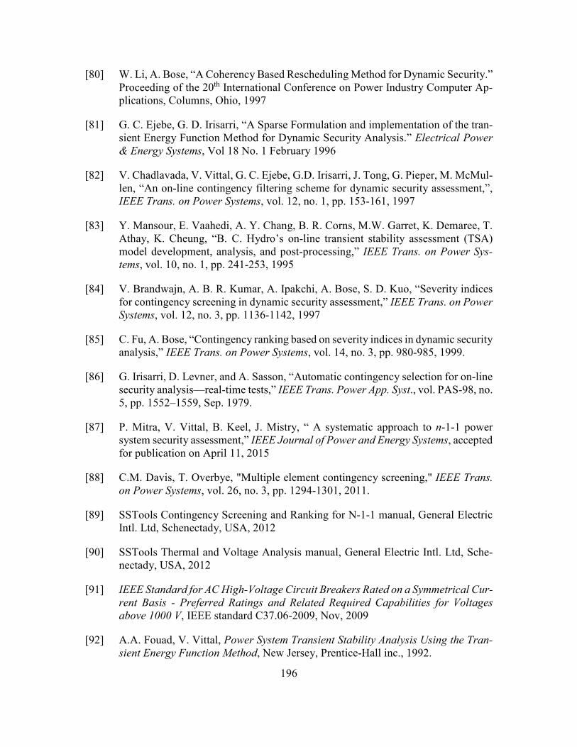
196
[80] W. Li, A. Bose, “A Coherency Based Rescheduling Method for Dynamic Security.”
Proceeding of the 20th International Conference on Power Industry Computer Ap-
plications, Columns, Ohio, 1997
[81] G. C. Ejebe, G. D. Irisarri, “A Sparse Formulation and implementation of the tran-
sient Energy Function Method for Dynamic Security Analysis.” Electrical Power
& Energy Systems, Vol 18 No. 1 February 1996
[82] V. Chadlavada, V. Vittal, G. C. Ejebe, G.D. Irisarri, J. Tong, G. Pieper, M. McMul-
len, “An on-line contingency filtering scheme for dynamic security assessment,”,
IEEE Trans. on Power Systems, vol. 12, no. 1, pp. 153-161, 1997
[83] Y. Mansour, E. Vaahedi, A. Y. Chang, B. R. Corns, M.W. Garret, K. Demaree, T.
Athay, K. Cheung, “B. C. Hydro’s on-line transient stability assessment (TSA)
model development, analysis, and post-processing,” IEEE Trans. on Power Sys-
tems, vol. 10, no. 1, pp. 241-253, 1995
[84] V. Brandwajn, A. B. R. Kumar, A. Ipakchi, A. Bose, S. D. Kuo, “Severity indices
for contingency screening in dynamic security assessment,” IEEE Trans. on Power
Systems, vol. 12, no. 3, pp. 1136-1142, 1997
[85] C. Fu, A. Bose, “Contingency ranking based on severity indices in dynamic security
analysis,” IEEE Trans. on Power Systems, vol. 14, no. 3, pp. 980-985, 1999.
[86] G. Irisarri, D. Levner, and A. Sasson, “Automatic contingency selection for on-line
security analysis—real-time tests,” IEEE Trans. Power App. Syst., vol. PAS-98, no.
5, pp. 1552–1559, Sep. 1979.
[87] P. Mitra, V. Vittal, B. Keel, J. Mistry, “ A systematic approach to n-1-1 power
system security assessment,” IEEE Journal of Power and Energy Systems, accepted
for publication on April 11, 2015
[88] C.M. Davis, T. Overbye, "Multiple element contingency screening," IEEE Trans.
on Power Systems, vol. 26, no. 3, pp. 1294-1301, 2011.
[89] SSTools Contingency Screening and Ranking for N-1-1 manual, General Electric
Intl. Ltd, Schenectady, USA, 2012
[90] SSTools Thermal and Voltage Analysis manual, General Electric Intl. Ltd, Sche-
nectady, USA, 2012
[91] IEEE Standard for AC High-Voltage Circuit Breakers Rated on a Symmetrical Cur-
rent Basis - Preferred Ratings and Related Required Capabilities for Voltages
above 1000 V, IEEE standard C37.06-2009, Nov, 2009
[92] A.A. Fouad, V. Vittal, Power System Transient Stability Analysis Using the Tran-
sient Energy Function Method, New Jersey, Prentice-Hall inc., 1992.

197
[93] D. Ernst, D. Ruiz-Vega, M. Pavella, P. Hirsch, D. Sobajic, "A unified approach to
transient stability contingency filtering, ranking and assessment," Proc. of Power
Engineering Society Summer Meeting, Vancouver, BC, 2001.
[94] O. Alsac, B. Stott, W. F. Tinney, “Sparsity-oriented compensation methods for
modified network solutions,” IEEE Trans. on Power Apparatus and Systems, vol
102, no. 5, pp. 1050-1060, Nov 1983
[95] V. Kolluri, S. Mandal, M. Y. Vaiman, M. M. Vaiman, S. Lee, and P. Hirsch, “Fast
fault screening approach to assessing transient stability in entergy’s power system,”
Proc. IEEE/PES General Meeting, Tampa, FL, Jun. 24-27, 2007, 2007
[96] Capitanescu, F., Martinez Ramos, J. L., Panciatici, P., Kirschen, D., Marano Mar-
colini, A., Platbrood, L., Wehenkel, L., “State-ofthe-art, challenges, and future
trends in security constrained optimal power flow,” Electric Power Systems Re-
search, 81(8), 1731-1741.
[97] K.W. Hedman, S.S. Oren, R. P. O’Neil, “A review of transmission switching and
network topology optimization,” Proc. of IEEE PES General Meeting 2011, pp. 1-
7, July 2011.
[98] M. S. Ardakani, X. Li, P. Balasubramanian, K. W. Hedman, M. A. Khorshand,
“Real-time contingency analysis with transmission switching on real power system
data,” IEEE Trans. on Power Systems, vol. 31, no. 3, pp. 2501-2502, 2015

198
APPENDIX A
WECC MODEL DESCRIPTION AND LOAD DATA
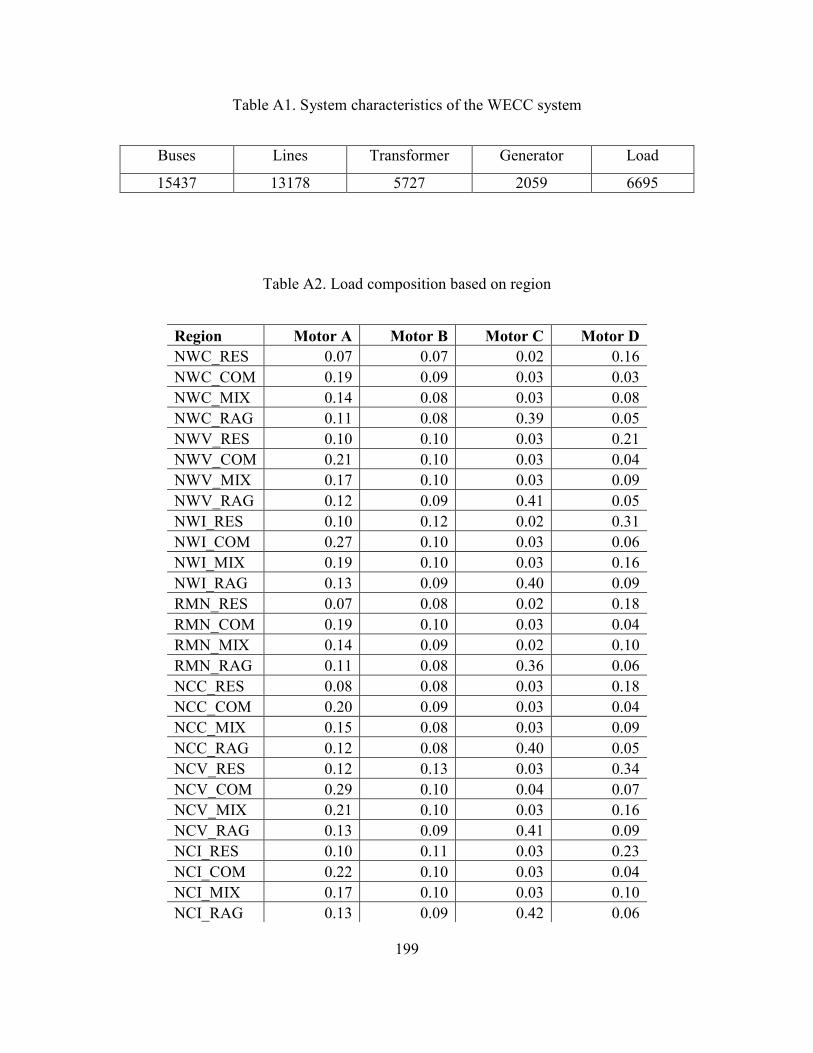
199
Table A1. System characteristics of the WECC system
Buses Lines Transformer Generator Load
15437 13178 5727 2059 6695
Table A2. Load composition based on region
Region Motor A Motor B Motor C Motor D
NWC_RES 0.07 0.07 0.02 0.16
NWC_COM 0.19 0.09 0.03 0.03
NWC_MIX 0.14 0.08 0.03 0.08
NWC_RAG 0.11 0.08 0.39 0.05
NWV_RES 0.10 0.10 0.03 0.21
NWV_COM 0.21 0.10 0.03 0.04
NWV_MIX 0.17 0.10 0.03 0.09
NWV_RAG 0.12 0.09 0.41 0.05
NWI_RES 0.10 0.12 0.02 0.31
NWI_COM 0.27 0.10 0.03 0.06
NWI_MIX 0.19 0.10 0.03 0.16
NWI_RAG 0.13 0.09 0.40 0.09
RMN_RES 0.07 0.08 0.02 0.18
RMN_COM 0.19 0.10 0.03 0.04
RMN_MIX 0.14 0.09 0.02 0.10
RMN_RAG 0.11 0.08 0.36 0.06
NCC_RES 0.08 0.08 0.03 0.18
NCC_COM 0.20 0.09 0.03 0.04
NCC_MIX 0.15 0.08 0.03 0.09
NCC_RAG 0.12 0.08 0.40 0.05
NCV_RES 0.12 0.13 0.03 0.34
NCV_COM 0.29 0.10 0.04 0.07
NCV_MIX 0.21 0.10 0.03 0.16
NCV_RAG 0.13 0.09 0.41 0.09
NCI_RES 0.10 0.11 0.03 0.23
NCI_COM 0.22 0.10 0.03 0.04
NCI_MIX 0.17 0.10 0.03 0.10
NCI_RAG 0.13 0.09 0.42 0.06
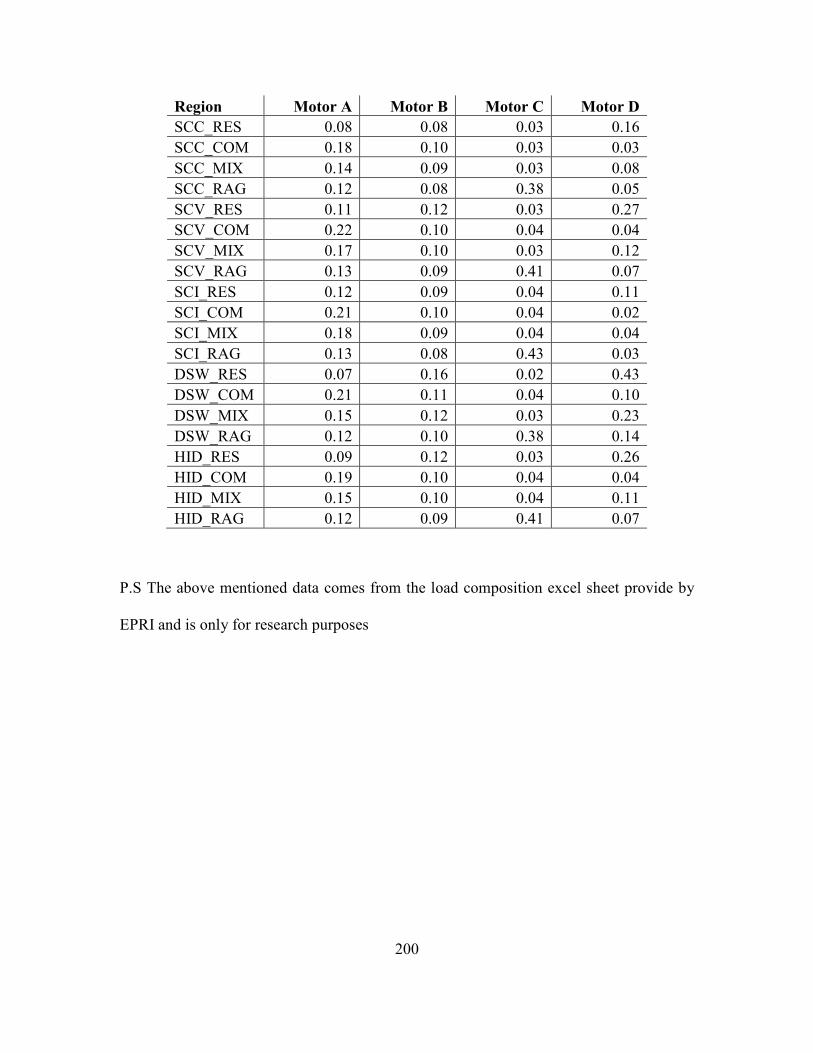
200
Region Motor A Motor B Motor C Motor D
SCC_RES 0.08 0.08 0.03 0.16
SCC_COM 0.18 0.10 0.03 0.03
SCC_MIX 0.14 0.09 0.03 0.08
SCC_RAG 0.12 0.08 0.38 0.05
SCV_RES 0.11 0.12 0.03 0.27
SCV_COM 0.22 0.10 0.04 0.04
SCV_MIX 0.17 0.10 0.03 0.12
SCV_RAG 0.13 0.09 0.41 0.07
SCI_RES 0.12 0.09 0.04 0.11
SCI_COM 0.21 0.10 0.04 0.02
SCI_MIX 0.18 0.09 0.04 0.04
SCI_RAG 0.13 0.08 0.43 0.03
DSW_RES 0.07 0.16 0.02 0.43
DSW_COM 0.21 0.11 0.04 0.10
DSW_MIX 0.15 0.12 0.03 0.23
DSW_RAG 0.12 0.10 0.38 0.14
HID_RES 0.09 0.12 0.03 0.26
HID_COM 0.19 0.10 0.04 0.04
HID_MIX 0.15 0.10 0.04 0.11
HID_RAG 0.12 0.09 0.41 0.07
P.S The above mentioned data comes from the load composition excel sheet provide by
EPRI and is only for research purposes
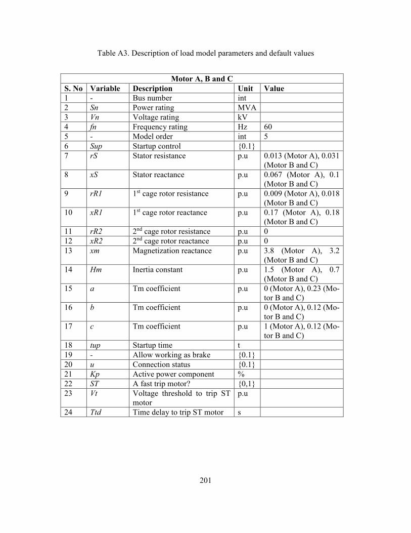
201
Table A3. Description of load model parameters and default values
Motor A, B and C
S. No Variable Description Unit Value
1 - Bus number int
2 Sn Power rating MVA
3 Vn Voltage rating kV
4 fn Frequency rating Hz 60
5 - Model order int 5
6 Sup Startup control {0.1}
7 rS Stator resistance p.u 0.013 (Motor A), 0.031
(Motor B and C)
8 xS Stator reactance p.u 0.067 (Motor A), 0.1
(Motor B and C)
9 rR1 1st cage rotor resistance p.u 0.009 (Motor A), 0.018
(Motor B and C)
10 xR1 1st cage rotor reactance p.u 0.17 (Motor A), 0.18
(Motor B and C)
11 rR2 2nd cage rotor resistance p.u 0
12 xR2 2nd cage rotor reactance p.u 0
13 xm Magnetization reactance p.u 3.8 (Motor A), 3.2
(Motor B and C)
14 Hm Inertia constant p.u 1.5 (Motor A), 0.7
(Motor B and C)
15 a Tm coefficient p.u 0 (Motor A), 0.23 (Mo-
tor B and C)
16 b Tm coefficient p.u 0 (Motor A), 0.12 (Mo-
tor B and C)
17 c Tm coefficient p.u 1 (Motor A), 0.12 (Mo-
tor B and C)
18 tup Startup time t
19 - Allow working as brake {0.1}
20 u Connection status {0.1}
21 Kp Active power component %
22 ST A fast trip motor? {0,1}
23 Vt Voltage threshold to trip ST
motor
p.u
24 Ttd Time delay to trip ST motor s

202
Motor D
S. No Variable Description Unit Unit
1 Vbrk Compressor breakdown voltage pu 0.86
2 Vstall Stall voltage pu 0.7
3 Tstall Time to stall sec 0.03
3
3 Rstall Stall resistance of the induction machine pu 0.12
4
4 Xstall Stall reactance of the induction machine pu 0.11
4
5 Kp1 Active power coefficient in state 1 in p.u P/p.u V 0
6 Np1 Active power exponent in state 1 1
7 Kq1 Reactive power coefficient in state 1 in p.u Q/p.u
V
6
8 Nq1 Reactive power exponent in state 1 2
9 Kp2 Active power coefficient in state 2 in p.u P/p.u V 12
10 Np2 Active power exponent in state 2 3.2
11 Kq2 Reactive power coefficient in state 2 in p.u Q/p.u
V
11
12 Nq2 Reactive power exponent in state 2 2.5
13 Kpf Active power frequency sensitivity in p.u P/p.u f 1
14 Kqf Reactive power frequency sensitivity in p.u
Q/p.u f
-3.3