linear programming
DESCRIPTION
Kagiso Trust's KT Classroom: Linear ProgrammingTRANSCRIPT
MATHEMATICS
Learner’s Study and
Revision Guide for
Grade 12
Linear Programming
Revision Notes, Exercises and Solution Hints by
Roseinnes Phahle
Examination Questions by the Department of Basic Education
Preparation for the Mathematics examination brought to you by Kagiso Trust
Contents
Unit 12
The language of linear programming problems 3
Feasuble region 4
The objective function/search lime 5
A tip on working out the mathematical expressions for the constraints 6
Exercise 12.1 7
Answer to Exercise 12.1 8
Examination questions with solution hints and answers 10
More questions from past examination papers 17
Answers 26
How to use this revision and study guide
1. Study the revision notes given at the beginning. The notes are interactive in that in some parts you are required to make a response based on your prior learning of the topic from your teacher in class or from a textbook. Furthermore, the notes cover all the Mathematics from Grade 10 to Grade 12.
2. “Warm-up” exercises follow the notes. Some exercises carry solution HINTS in the answer section. Do not read the answer or hints until you have tried to work out a question and are having difficulty.
3. The notes and exercises are followed by questions from past examination papers.
4. The examination questions are followed by blank spaces or boxes inside a table. Do the working out of the question inside these spaces or boxes.
5. Alongside the blank boxes are HINTS in case you have difficulty solving a part of the question. Do not read the hints until you have tried to work out the question and are having difficulty.
6. What follows next are more questions taken from past examination papers.
7. Answers to the extra past examination questions appear at the end. Some answers carry HINTS and notes to enrich your knowledge.
8. Finally, don’t be a loner. Work through this guide in a team with your classmates.
Linear Programming
3
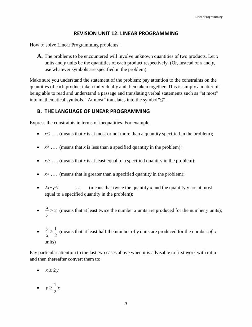
REVISION UNIT 12: LINEAR PROGRAMMING
How to solve Linear Programming problems:
A. The problems to be encountered will involve unknown quantities of two products. Let x units and y units be the quantities of each product respectively. (Or, instead of x and y, use whatever symbols are specified in the problem).
Make sure you understand the statement of the problem: pay attention to the constraints on the quantities of each product taken individually and then taken together. This is simply a matter of being able to read and understand a passage and translating verbal statements such as “at most” into mathematical symbols. “At most” translates into the symbol ""≤ .
B. THE LANGUAGE OF LINEAR PROGRAMMING
Express the constraints in terms of inequalities. For example:
• x≤ …. (means that x is at most or not more than a quantity specified in the problem);
• x< …. (means that x is less than a specified quantity in the problem);
• x≥ …. (means that x is at least equal to a specified quantity in the problem);
• x> …. (means that is greater than a specified quantity in the problem);
• 2x+y≤ …. (means that twice the quantity x and the quantity y are at most equal to a specified quantity in the problem);
• 2≥yx (means that at least twice the number x units are produced for the number y units);
• 21
≥xy (means that at least half the number of y units are produced for the number of x
units)
Pay particular attention to the last two cases above when it is advisable to first work with ratio and then thereafter convert them to:
• yx 2≥
• xy21
≥
Preparation for the Mathematics examination brought to you by Kagiso Trust
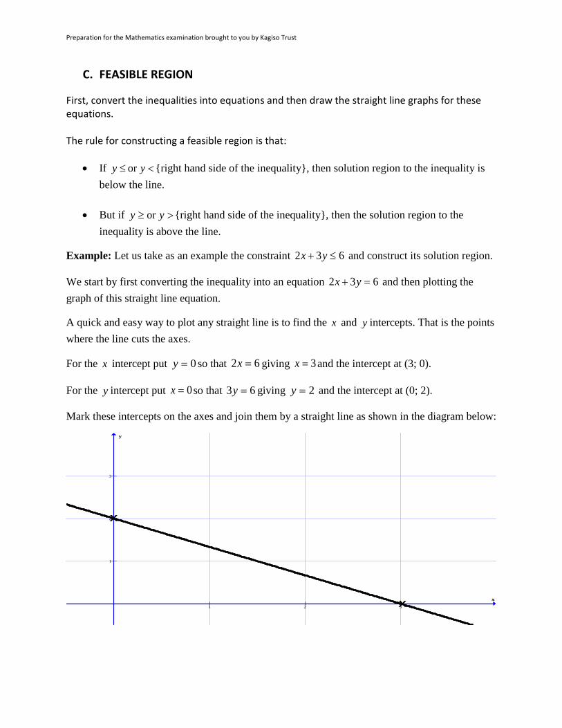
C. FEASIBLE REGION
First, convert the inequalities into equations and then draw the straight line graphs for these equations. The rule for constructing a feasible region is that:
• If <≤ yy or {right hand side of the inequality}, then solution region to the inequality is below the line.
• But if >≥ yy or {right hand side of the inequality}, then the solution region to the inequality is above the line.
Example: Let us take as an example the constraint 632 ≤+ yx and construct its solution region.
We start by first converting the inequality into an equation 632 =+ yx and then plotting the graph of this straight line equation.
A quick and easy way to plot any straight line is to find the x and y intercepts. That is the points where the line cuts the axes.
For the x intercept put 0=y so that 62 =x giving 3=x and the intercept at (3; 0).
For the y intercept put 0=x so that 63 =y giving 2=y and the intercept at (0; 2).
Mark these intercepts on the axes and join them by a straight line as shown in the diagram below:
1 2 3
1
2
3
x
y
X
X
Linear Programming
5
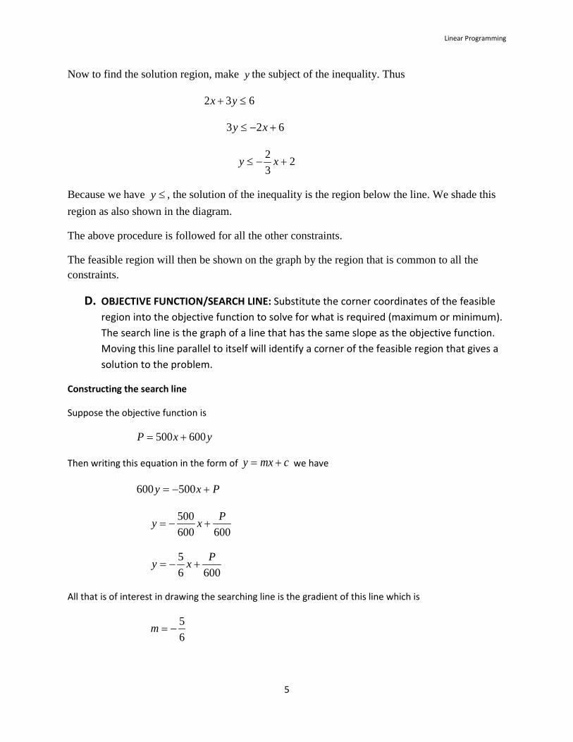
Now to find the solution region, make y the subject of the inequality. Thus
632 ≤+ yx
623 +−≤ xy
232
+−≤ xy
Because we have ≤y , the solution of the inequality is the region below the line. We shade this region as also shown in the diagram.
The above procedure is followed for all the other constraints.
The feasible region will then be shown on the graph by the region that is common to all the constraints.
D. OBJECTIVE FUNCTION/SEARCH LINE: Substitute the corner coordinates of the feasible region into the objective function to solve for what is required (maximum or minimum). The search line is the graph of a line that has the same slope as the objective function. Moving this line parallel to itself will identify a corner of the feasible region that gives a solution to the problem.
Constructing the search line
Suppose the objective function is
yxP 600500 +=
Then writing this equation in the form of cmxy += we have
Pxy +−= 500600
600600
500 Pxy +−=
6006
5 Pxy +−=
All that is of interest in drawing the searching line is the gradient of this line which is
65
−=m
Preparation for the Mathematics examination brought to you by Kagiso Trust
The search line is given by any of the infinite number of lines with gradient = 65
− .
To show the search line, all we need to do is to draw a line with this gradient.
Moving this line parallel to itself, the coordinates for a maximum of the objective function will be given by the coordinates of the corner (vertex) of the feasible region furthest from the origin.
In cost problems, the solution may be a given by a minimum value of the objective function. In this case the coordinates for a minimum of the objective function will be given by the coordinates of the point of the corner of the feasible region nearest to the origin.
E. A TIP ON WORKING OUT MATHEMATICAL EXPRESSIONS FOR THE CONSTRAINTS
Most students find it difficult to convert “word” problems into mathematical expressions and so are put off answering linear programming problems because these are “word” problems. Linear programming at Grade 12 is first and foremost about translating ordinary language into mathematical symbols. To help with this translation this chapter began by giving you a list of symbols and their meanings used to express constraints. Have another look at that list.
To help you even further in turning the words of linear programming problems into constraints expressed in terms of mathematical symbols, setting up a table is highly recommended. The table will be of the form:
Quantities
Other information
Other informatiom
Cost or Profit Function
Variable No 1 x Constraints Variable No 2 y Constraints Constraints Constraints Constraints C or P =
It is a table like this you must draw and fill in, as will be illustrated in the example bel
How you must go about solving a Linear programming problem is now demonstrated below.
Example: Mme Mamabolo makes two types of shirts. One is an Afro shirt that requires 21
an hour to
make. The other is a Madiba shirt that requires one hour to make. The time available for making the shirts is not more than 8 hours a day. To keep her business going Mme Mamabolo needs to produce at least one and not more than 6 Afro shirts a day; and at most 6 and not less than 2 Madiba shirts a day. However, market demand is for at least 3 Madiba shirts and one Afro shirt a day.
If the Afro shirt retails at R300 and the Madiba shirt at R800, how many of each should be produced in a day in order to maximize profit.
Linear Programming
7
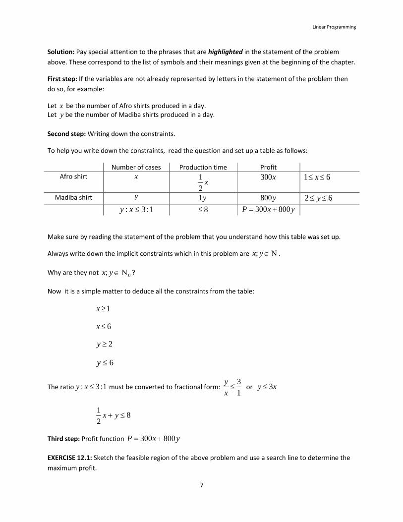
Solution: Pay special attention to the phrases that are highlighted in the statement of the problem above. These correspond to the list of symbols and their meanings given at the beginning of the chapter.
First step: If the variables are not already represented by letters in the statement of the problem then do so, for example:
Let x be the number of Afro shirts produced in a day. Let y be the number of Madiba shirts produced in a day. Second step: Writing down the constraints.
To help you write down the constraints, read the question and set up a table as follows:
Number of cases Production time Profit Afro shirt x
x21
x300 61 ≤≤ x
Madiba shirt y y1 y800 62 ≤≤ y 1:3: ≤xy 8≤ yxP 800300 +=
Make sure by reading the statement of the problem that you understand how this table was set up.
Always write down the implicit constraints which in this problem are Ν∈yx; .
Why are they not 0; Ν∈yx ?
Now it is a simple matter to deduce all the constraints from the table:
1≥x
6≤x
2≥y
6≤y
The ratio 1:3: ≤xy must be converted to fractional form: 13
≤xy
or xy 3≤
821
≤+ yx
Third step: Profit function yxP 800300 += EXERCISE 12.1: Sketch the feasible region of the above problem and use a search line to determine the maximum profit.
Preparation for the Mathematics examination brought to you by Kagiso Trust
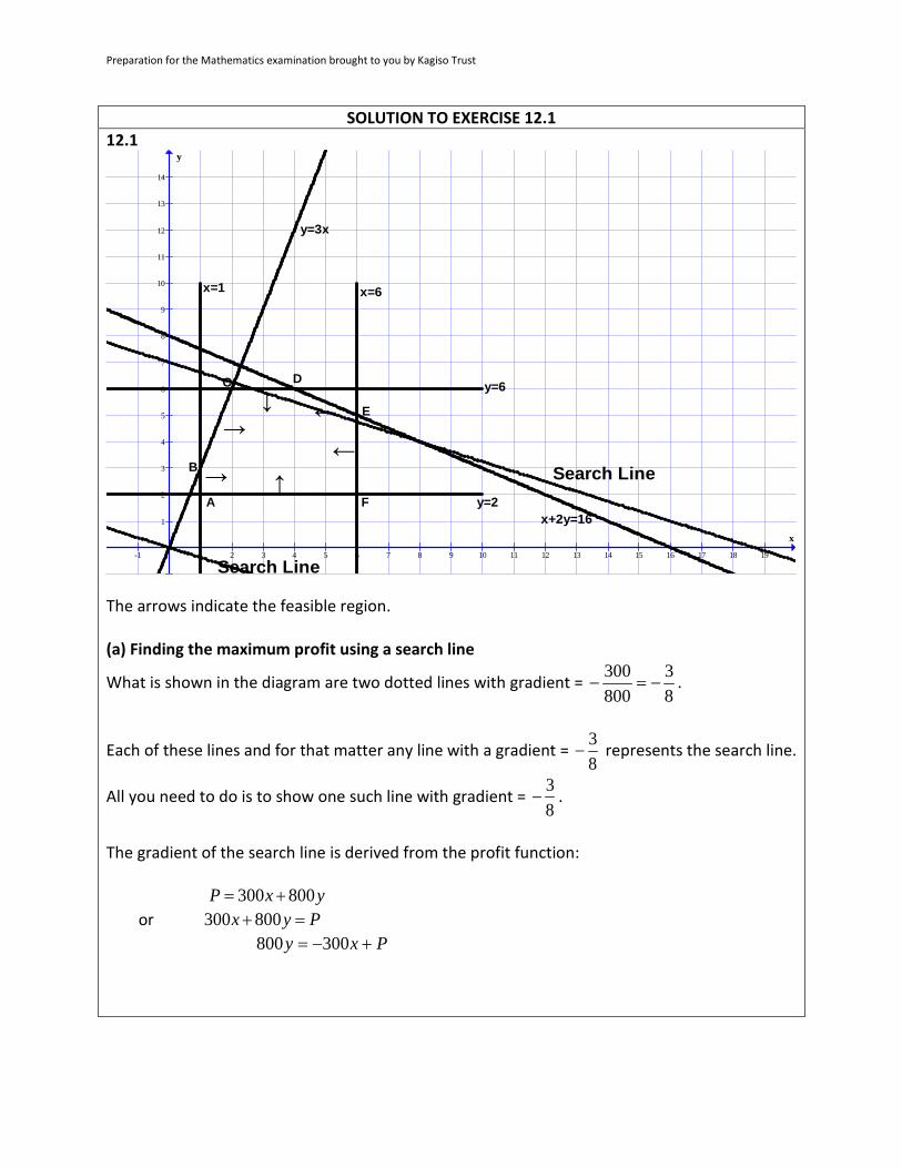
SOLUTION TO EXERCISE 12.1 12.1
-1 1 2 3 4 5 6 7 8 9 10 11 12 13 14 15 16 17 18 19
1
2
3
4
5
6
7
8
9
10
11
12
13
14
x
y
x+2y=16
y=3x
x=6x=1
y=6
y=2A
B
C D
E
F
←←↓
→
→
↑ Search Line
Search Line The arrows indicate the feasible region. (a) Finding the maximum profit using a search line
What is shown in the diagram are two dotted lines with gradient = 83
800300
−=− .
Each of these lines and for that matter any line with a gradient = 83
− represents the search line.
All you need to do is to show one such line with gradient = 83
− .
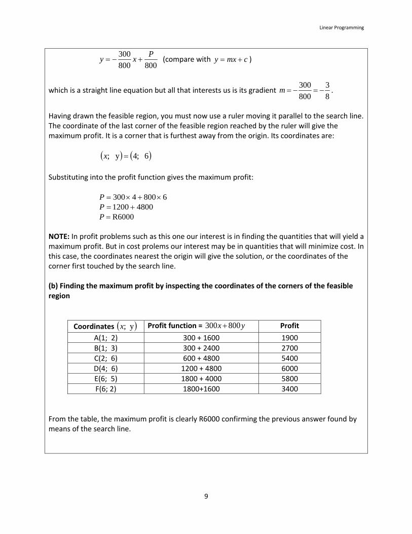
The gradient of the search line is derived from the profit function: yxP 800300 += or Pyx =+800300 Pxy +−= 300800
Linear Programming
9
800800
300 Pxy +−= (compare with cmxy += )
which is a straight line equation but all that interests us is its gradient 83
800300
−=−=m .
Having drawn the feasible region, you must now use a ruler moving it parallel to the search line. The coordinate of the last corner of the feasible region reached by the ruler will give the maximum profit. It is a corner that is furthest away from the origin. Its coordinates are: ( ) ( )6 ;4y ; =x Substituting into the profit function gives the maximum profit: 68004300 ×+×=P 48001200 +=P R6000=P NOTE: In profit problems such as this one our interest is in finding the quantities that will yield a maximum profit. But in cost prolems our interest may be in quantities that will minimize cost. In this case, the coordinates nearest the origin will give the solution, or the coordinates of the corner first touched by the search line. (b) Finding the maximum profit by inspecting the coordinates of the corners of the feasible region
Coordinates ( )y ;x Profit function = yx 800300 + Profit A(1; 2) 300 + 1600 1900 B(1; 3) 300 + 2400 2700 C(2; 6) 600 + 4800 5400 D(4; 6) 1200 + 4800 6000 E(6; 5) 1800 + 4000 5800 F(6; 2) 1800+1600 3400
From the table, the maximum profit is clearly R6000 confirming the previous answer found by means of the search line.
Preparation for the Mathematics examination brought to you by Kagiso Trust
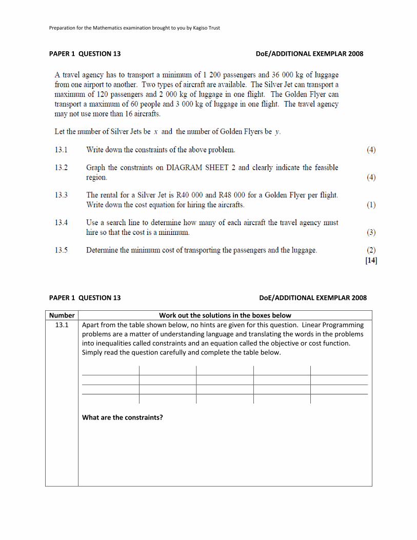
PAPER 1 QUESTION 13 DoE/ADDITIONAL EXEMPLAR 2008
PAPER 1 QUESTION 13 DoE/ADDITIONAL EXEMPLAR 2008
Number Work out the solutions in the boxes below 13.1 Apart from the table shown below, no hints are given for this question. Linear Programming
problems are a matter of understanding language and translating the words in the problems into inequalities called constraints and an equation called the objective or cost function. Simply read the question carefully and complete the table below.
What are the constraints?
Linear Programming
11
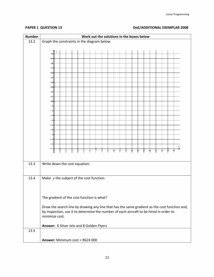
PAPER 1 QUESTION 13 DoE/ADDITIONAL EXEMPLAR 2008
Number Work out the solutions in the boxes below 13.2
Graph the constraints in the diagram below.
13.3 Write down the cost equation:
13.4 Make y the subject of the cost function. The gradient of the cost function is what? Draw the search line by drawing any line that has the same gradient as the cost function and, by inspection, use it to determine the number of each aircraft to be hired in order to minimize cost. Answer: 6 Silver Jets and 8 Golden Flyers
13.5 Answer: Minimum cost = R624 000
Preparation for the Mathematics examination brought to you by Kagiso Trust
PAPER 1 QUESTION 11 DoE/NOVEMBER 2008
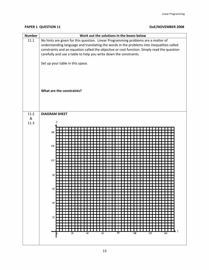
Linear Programming
13
PAPER 1 QUESTION 11 DoE/NOVEMBER 2008
Number Work out the solutions in the boxes below 11.1 No hints are given for this question. Linear Programming problems are a matter of
understanding language and translating the words in the problems into inequalities called constraints and an equation called the objective or cost function. Simply read the question carefully and use a table to help you write down the constraints. Set up your table in this space. What are the constraints?
11.2 &
11.3
DIAGRAM SHEET
Preparation for the Mathematics examination brought to you by Kagiso Trust
Number Work out the solutions in the boxes below 11.4 Write down the profit equation:
11.5 Make y the subject of the profit function. So what is the gradient of this new profit function? Draw any line that has the same gradient as the profit function and show this line on the graph above. This will be the search line. Answer: Maximum at (20; 75)
11.6 Make y the subject of the new profit function. So what is the gradient of this new profit function? Compare it with the gradient of the original profit function in 11.4. Or draw its search line on your diagram in order to find a reason to the conclusion you make. What do you conclude in terms of the optimal solution?
Linear Programming
15
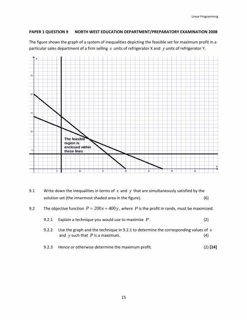
PAPER 1 QUESTION 9 NORTH WEST EDUCATION DEPARTMENT/PREPARATORY EXAMINATION 2008
The figure shows the graph of a system of inequalities depicting the feasible set for maximum profit in a particular sales department of a firm selling x units of refrigerator X and y units of refrigerator Y.
5 10 15 20 25 30 35
5
10
15
20
25
x
y
The feasible region is enclosed withinthese lines
9.1 Write down the inequalities in terms of x and y that are simultaneously satisfied by the
solution set (the innermost shaded area in the figure). (6)
9.2 The objective function yxP 400200 += , where P is the profit in rands, must be maximized.
9.2.1 Explain a technique you would use to maximize P . (2)
9.2.2 Use the graph and the technique in 9.2.1 to determine the corresponding values of x and y such that P is a maximum. (4)
9.2.3 Hence or otherwise determine the maximum profit. (2) [14]
Preparation for the Mathematics examination brought to you by Kagiso Trust
PAPER 1 QUESTION 9 NORTH WEST EDUCATION DEPARTMENT/PREPARATORY EXAMINATION 2008
Number Hints and answers Work out the solutions in the boxes below 9.1 Find the equations of all the straight
lines shown in the figure. Convert these equations into constraints. Remember that ≤ is the constraint for a region under a line; and ≥ is the constraint for a region above a line.
Put you answers in this box:
9.2.1 Write the equation of the profit function in the form y = Answer: y =
Your answer must explain how you would use the gradient of the profit function. Explanation:
9.2.2 Carry out what you have explained. There is more than one solution. Explain why?
Explain here why there is more than one solution:
9.2.3 Substitute any of the results you found in 9.2.2 into the profit function. Answer:
Linear Programming
17
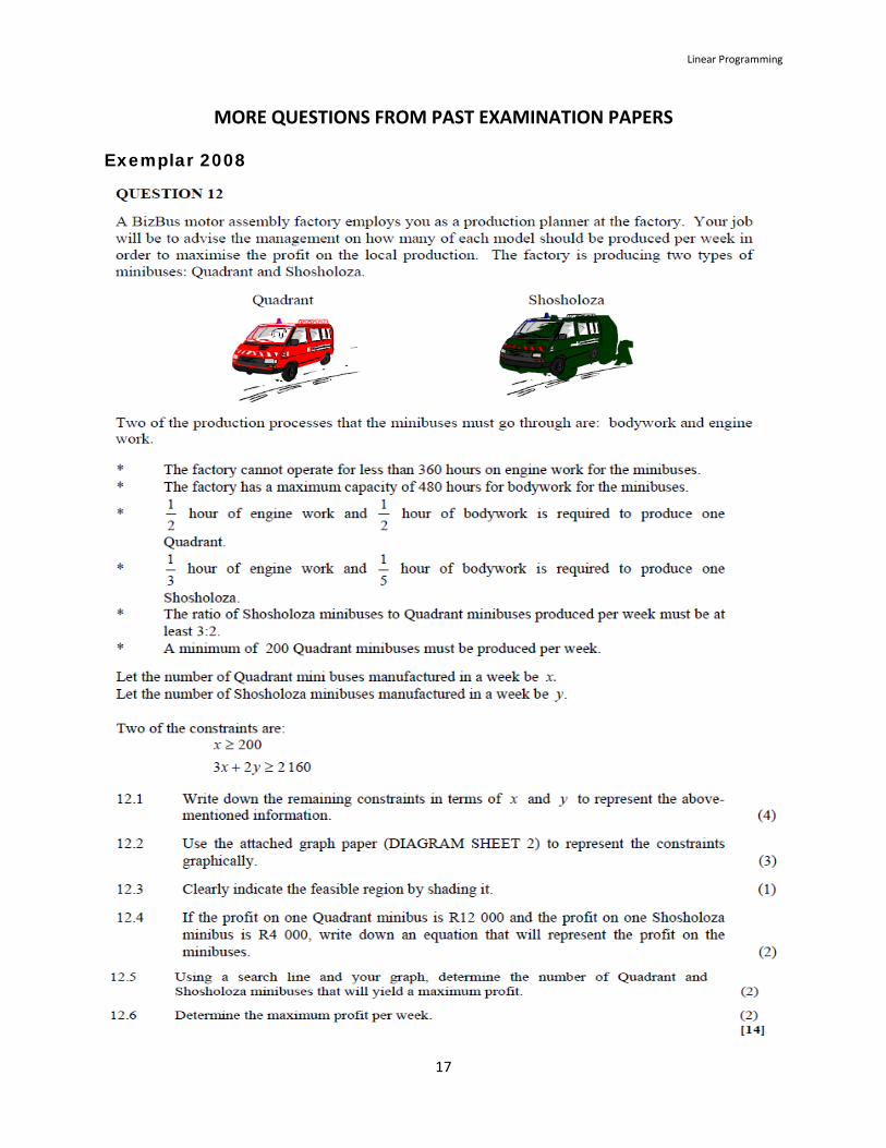
MORE QUESTIONS FROM PAST EXAMINATION PAPERS
Exemplar 2008
Preparation for the Mathematics examination brought to you by Kagiso Trust
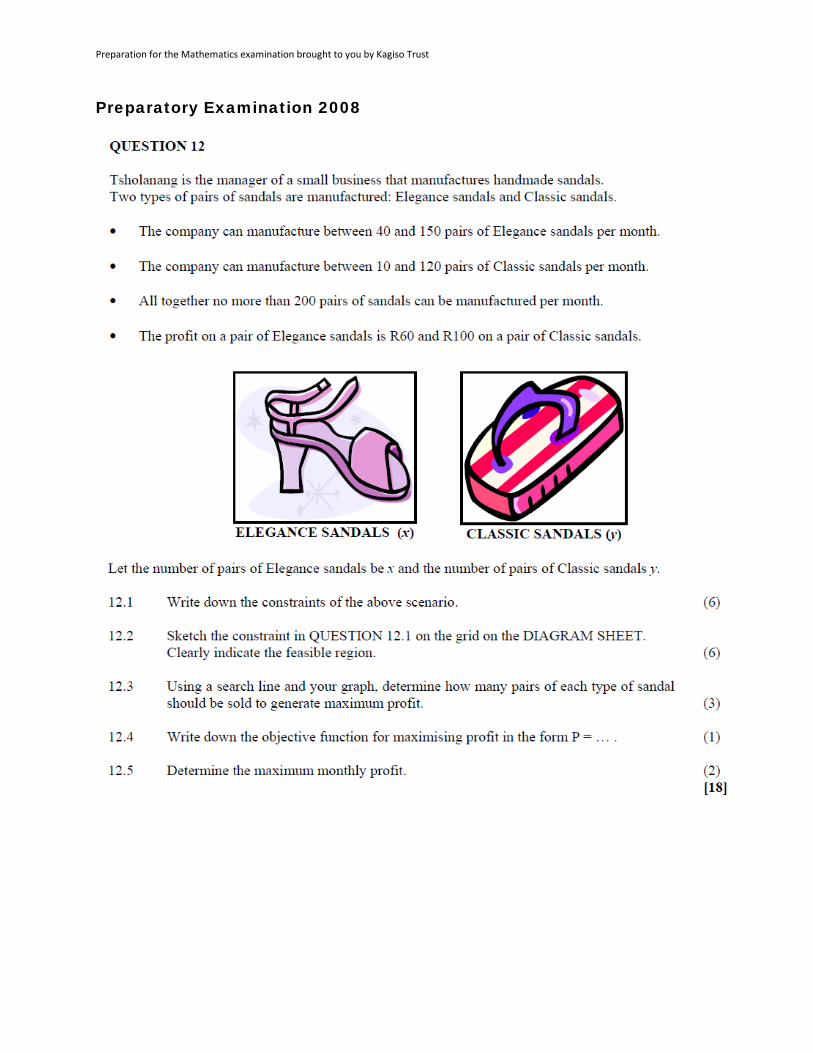
Preparatory Examination 2008
Linear Programming
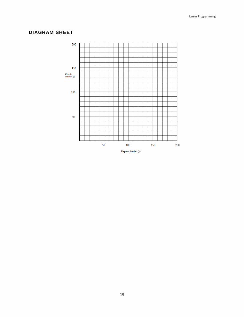
19
DIAGRAM SHEET
Preparation for the Mathematics examination brought to you by Kagiso Trust
November 2008
Linear Programming
21
Feb – March 2009
Preparation for the Mathematics examination brought to you by Kagiso Trust
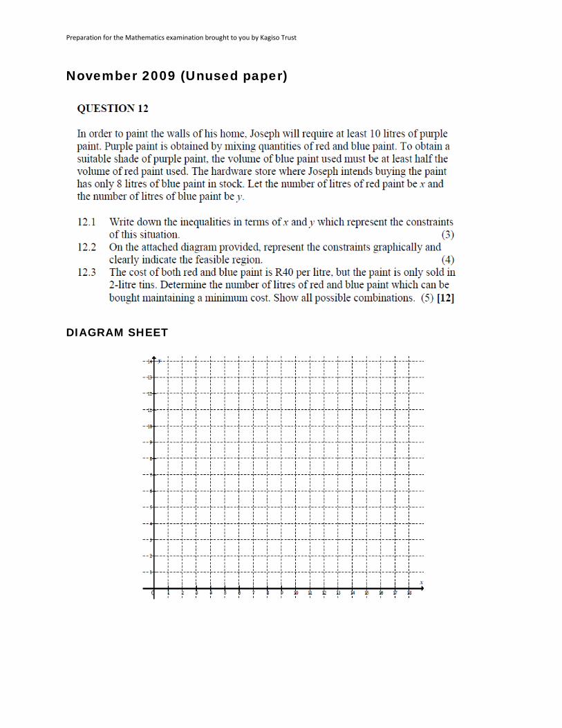
November 2009 (Unused paper)
DIAGRAM SHEET
Linear Programming
23
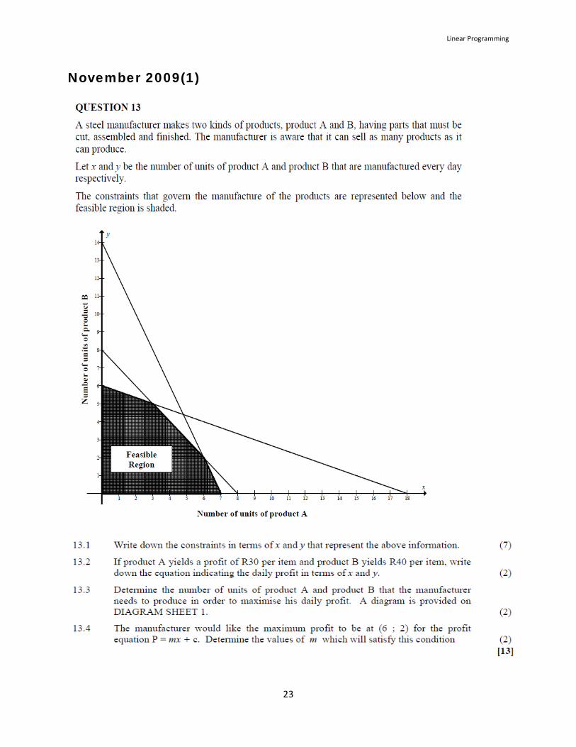
November 2009(1)
Preparation for the Mathematics examination brought to you by Kagiso Trust
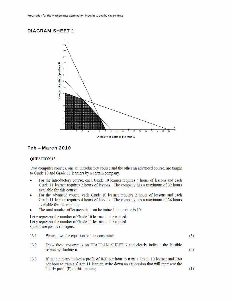
DIAGRAM SHEET 1
Feb – March 2010
Linear Programming
25
DIAGRAM SHEET 3
Preparation for the Mathematics examination brought to you by Kagiso Trust
ANSWERS
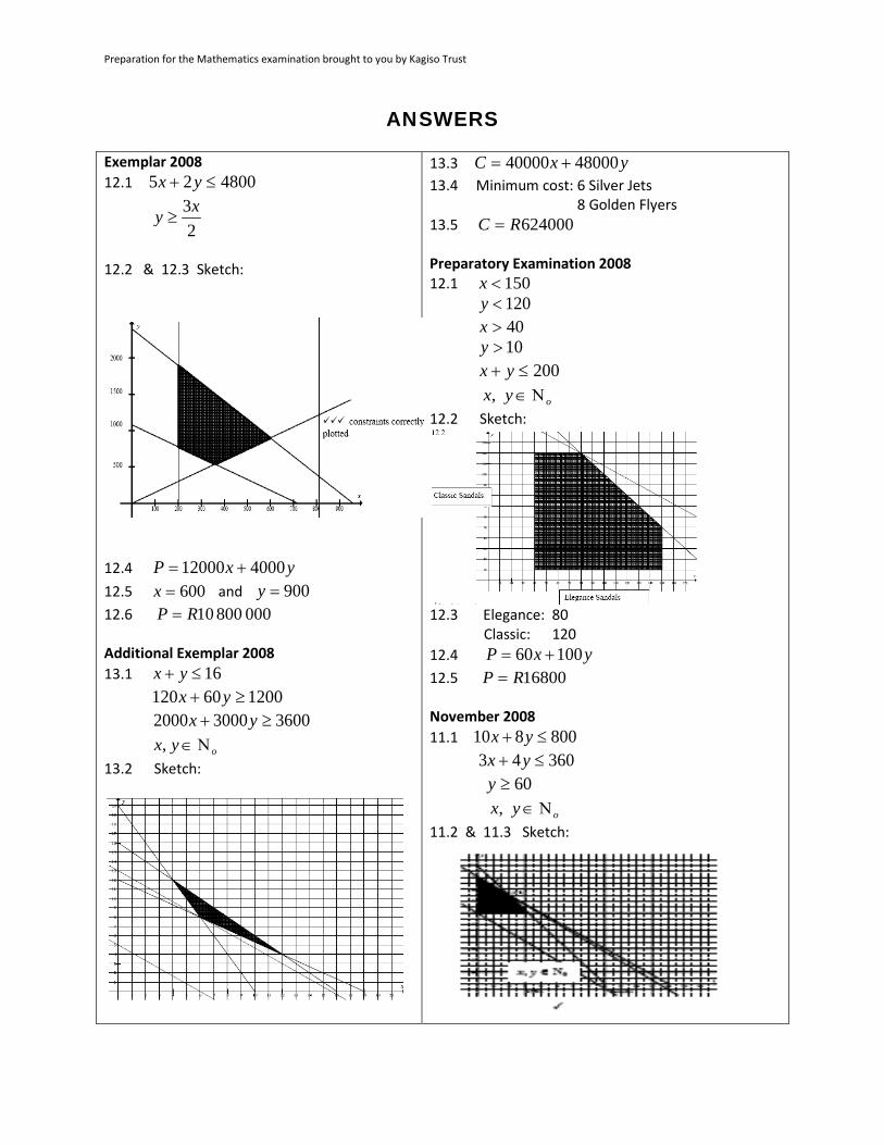
Exemplar 2008 12.1 480025 ≤+ yx
2
3xy ≥
12.2 & 12.3 Sketch:
12.4 yxP 400012000 += 12.5 600=x and 900=y 12.6 000 800 10RP = Additional Exemplar 2008 13.1 16≤+ yx 120060120 ≥+ yx 360030002000 ≥+ yx oyx Ν∈ , 13.2 Sketch:
13.3 yxC 4800040000 += 13.4 Minimum cost: 6 Silver Jets 8 Golden Flyers 13.5 624000RC = Preparatory Examination 2008 12.1 150<x 120<y 40>x 10>y 200≤+ yx oyx Ν∈ , 12.2 Sketch:
12.3 Elegance: 80 Classic: 120 12.4 yxP 10060 += 12.5 16800RP = November 2008 11.1 800810 ≤+ yx 36043 ≤+ yx 60≥y oyx Ν∈ , 11.2 & 11.3 Sketch:
Linear Programming
27
11.4 yxP 250200 += 11.5 Maximum at (20; 75)
11.6 43
−=m
Thus the profit function has the same gradient as the constraint
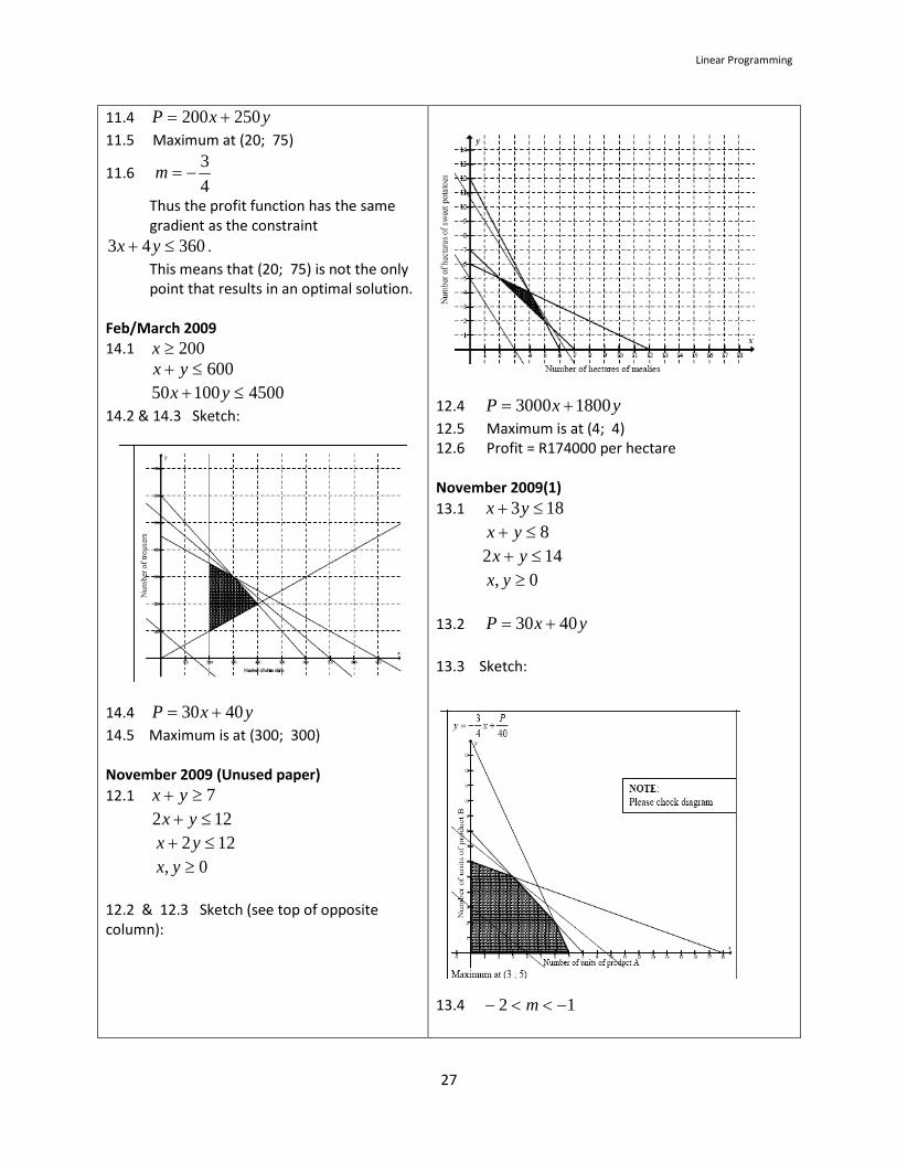
36043 ≤+ yx . This means that (20; 75) is not the only point that results in an optimal solution. Feb/March 2009 14.1 200≥x 600≤+ yx 450010050 ≤+ yx 14.2 & 14.3 Sketch:
14.4 yxP 4030 += 14.5 Maximum is at (300; 300) November 2009 (Unused paper) 12.1 7≥+ yx 122 ≤+ yx 122 ≤+ yx 0, ≥yx 12.2 & 12.3 Sketch (see top of opposite column):
12.4 yxP 18003000 += 12.5 Maximum is at (4; 4) 12.6 Profit = R174000 per hectare November 2009(1) 13.1 183 ≤+ yx 8≤+ yx 142 ≤+ yx 0, ≥yx 13.2 yxP 4030 += 13.3 Sketch:
13.4 12 −<<− m
Preparation for the Mathematics examination brought to you by Kagiso Trust
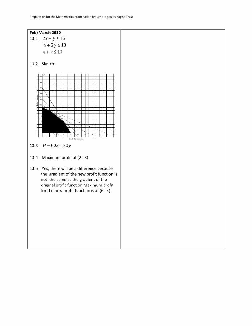
Feb/March 2010 13.1 162 ≤+ yx 182 ≤+ yx 10≤+ yx 13.2 Sketch:
13.3 yxP 8060 += 13.4 Maximum profit at (2; 8) 13.5 Yes, there will be a difference because the gradient of the new profit function is not the same as the gradient of the original profit function Maximum profit for the new profit function is at (6; 4).