linear odes: an algebraic perspective - impa · linear odes: an algebraic perspective letterio...
TRANSCRIPT
Linear ODEs: an Algebraic Perspective


Publicações Matemáticas
Linear ODEs: an Algebraic Perspective
Letterio Gatto Politecnico di Torino
impa
Copyright 2012 by Letterio Gatto
Impresso no Brasil / Printed in Brazil
Capa: Noni Geiger / Sérgio R. Vaz
Publicações Matemáticas • Introdução à Topologia Diferencial – Elon Lages Lima
• Criptografia, Números Primos e Algoritmos – Manoel Lemos
• Introdução à Economia Dinâmica e Mercados Incompletos – Aloísio Araújo
• Conjuntos de Cantor, Dinâmica e Aritmética – Carlos Gustavo Moreira
• Geometria Hiperbólica – João Lucas Marques Barbosa
• Introdução à Economia Matemática – Aloísio Araújo
• Superfícies Mínimas – Manfredo Perdigão do Carmo
• The Index Formula for Dirac Operators: an Introduction – Levi Lopes de Lima
• Introduction to Symplectic and Hamiltonian Geometry – Ana Cannas da Silva
• Primos de Mersenne (e outros primos muito grandes) – Carlos Gustavo T. A. Moreira e Nicolau
Saldanha
• The Contact Process on Graphs – Márcia Salzano
• Canonical Metrics on Compact almost Complex Manifolds – Santiago R. Simanca
• Introduction to Toric Varieties – Jean-Paul Brasselet
• Birational Geometry of Foliations – Marco Brunella
• Introdução à Teoria das Probabilidades – Pedro J. Fernandez
• Teoria dos Corpos – Otto Endler
• Introdução à Dinâmica de Aplicações do Tipo Twist – Clodoaldo G. Ragazzo, Mário J. Dias
Carneiro e Salvador Addas Zanata
• Elementos de Estatística Computacional usando Plataformas de Software Livre/Gratuito –
Alejandro C. Frery e Francisco Cribari-Neto
• Uma Introdução a Soluções de Viscosidade para Equações de Hamilton-Jacobi – Helena J.
Nussenzveig Lopes, Milton C. Lopes Filho
• Elements of Analytic Hypoellipticity – Nicholas Hanges
• Métodos Clássicos em Teoria do Potencial – Augusto Ponce
• Variedades Diferenciáveis – Elon Lages Lima
• O Método do Referencial Móvel – Manfredo do Carmo
• A Student's Guide to Symplectic Spaces, Grassmannians and Maslov Index – Paolo Piccione e
Daniel Victor Tausk
• Métodos Topológicos en el Análisis no Lineal – Pablo Amster
• Tópicos em Combinatória Contemporânea – Carlos Gustavo Moreira e Yoshiharu Kohayakawa
• Uma Iniciação aos Sistemas Dinâmicos Estocásticos – Paulo Ruffino
• Compressive Sensing – Adriana Schulz, Eduardo A.B.. da Silva e Luiz Velho
• O Teorema de Poncelet – Marcos Sebastiani
• Cálculo Tensorial – Elon Lages Lima
• Aspectos Ergódicos da Teoria dos Números – Alexander Arbieto, Carlos Matheus e C. G. Moreira
• A Survey on Hiperbolicity of Projective Hypersurfaces – Simone Diverio e Erwan Rousseau
• Algebraic Stacks and Moduli of Vector Bundles – Frank Neumann
• O Teorema de Sard e suas Aplicações – Edson Durão Júdice
• Tópicos de Mecânica Clássica – Artur Lopes
• Holonomy Groups in Riemannian Geometry – Andrew Clark e Bianca Santoro
• Linear ODEs:an Algebraic Perspective - Letterio Gatto
IMPA - [email protected] - http://www.impa.br - ISBN: 978-85-244-0347-7
“FolhaRosto˙Letterio”2012/10/10page 2
i
i
i
i
i
i
i
i
- Letterio Gatto -
Dipartimento di Scienze Matematiche
Politecnico di Torino
Linear ODEs: an AlgebraicPerspective
Salvador – Bahia, Brazil – July 15 to 20, 2012

“EscoAlgtot˙New”2012/10/10page
i
i
i
i
i
i
i
i
To Aron Simis, on the occasion of his seventieth birthday

“EscoAlgtot˙New”2012/10/10page
i
i
i
i
i
i
i
i
“EscoAlgtot˙New”2012/10/10page
i
i
i
i
i
i
i
i
Preface
This booklet was intended to provide a minimum of ready-to-usereferences for the minicourse given by the author during the XXIIEscola de Algebra (40 Anos), held in Salvador de Bahia (July 2012).The purpose of these lecture notes is twofold. On one hand theyaim to introduce and advertise a natural, flexible and elegant purelycombinatorial–algebraic approach to the well-known classical theoryof linear ODEs withæ constant coefficients (Chapter 3), and to in-troduce generalised Wronskians associated to a fundamental systemof solutions (Chapter 4). Elementary applications will be shown, e.g.to the computation of the exponential of a square matrix withoutreducing to the Jordan normal form (Chapter 5). On the other handit wishes to bring to the fore a number of relationships with otherbranches of mathematics. Examples include the theory of symmetricfunctions (Example 2.1.3), the theory of universal decomposition al-gebras associated to a polynomial (Example 3.2.8 and Remark 6.1.8),derivations of the exterior algebra of a free module (Chapter 6), D-modules (Example 3.2.3), Schubert calculus for the complex Grass-mannian (Section 6.2), boson–fermion correspondence in the repre-sentation theory of the Heisenberg or the Virasoro algebra, the latterseen as an infinite–dimensional analogue of Poincare’s duality for thecomplex Grassmannians. The present exposition is totally inspiredby the paper [18] and must be considered an expanded version of it.
The level of the exposition is elementary, given that more thanseventy percent of the material can be followed with a basic under-standing of polynomial algebras and the Leibniz rule for the productof two differentiable functions. More advanced topics, like SchubertCalculus or the bosonic representation of the oscillator algebra have
“EscoAlgtot˙New”2012/10/10page
i
i
i
i
i
i
i
i
been only sketched in the last two chapters. A deeper knowledge ofthose subjects is not necessary for the purposes of the minicourse, asthey have been treated just to provide further examples to certify thesurprising ubiquity of the Jacobi-Trudy formula in mathematics.
The present lecture notes have been written on a short notice,so they will certainly contain misprints and omissions and possiblysome mistakes. Corrections and/or integrations can be found in theauthor’s web page at the url
http://calvino.polito.it/~gatto/public/XXIIEA/bahia.htm
ACKNOWLEDGMENTS. I wish to express my warmest feelingof gratitude to the Scientific Committee of the XXII Algebra Meet-ing, 40th anniversary, for giving him the opportunity to teach a mini-course on this subject, as well as to the Organizing Committee forproviding excellent stay conditions. A distinguished mention is dueto the Chairman of the Organizing Committee, Thierry Petit Lobao,for his careful assistance and his precious and friendly support. Itis also a pleasure to thank Parham Salehyan, who made possible alonger stay in Brasil for a collaboration related with the topics of thisbooklet.
Very special thanks are due to Inna Scherbak, the ideal coau-thor of these notes, who generously shared her insight and helpedme with many advises. I also thank Caterina Cumino and TaıseSantiago Mozzato for many discussions and my special friend SimonChiossi not only for enlightening discussions but especially for hisconstant encouragement. For the last sketchy chapter of these notesI am deeply indebted to Maxim Kazarian, from whom I first learnedabout the boson–fermion correspondence. For the friendly and carefulreading of the notes and for pointing me misprints and some mistake,I want to thank Peter Malcom Johnson. I am also indebted with Pro-fessor Louis Rowen for questions and remarks during his patient andstimulating presence to my lectures in Salvador, although they werein portuguese.
I am very grateful to Paolo Piccione and Paulo Sad for their gen-erous and encouraging support, as well as to the Instituto Nacionalde Matematica Pura e Aplicada do Rio de Janeiro, that allowed theinclusion of the present work within the collection of Monografiasde Matematica do IMPA. Many thanks are due to Rogerio Dias
“EscoAlgtot˙New”2012/10/10page
i
i
i
i
i
i
i
i
Trindade for his careful job preparing the final electronic version ofthe manuscript.
This work has been partially sponsored by the italian GNSAGA1-INDAM2, the PRIN3 “Geometria sulle Varieta Algebriche” (coordi-nated by A. Verra), by FAPESP4 processo n. 2012/02869-1, by Fil-ters srl (Scalenghe, TO) and the coffee brand Curt’eNiro (Pianezza,TO).
Estas notas de aula sao dedicadas ao Aron Simis, por ocasiaodo septuagesimo aniversario dele, desejando-lhe mais outros setentaanos de feliz atividade matematica.
Sangano, 23 de Maio 2012
1Gruppo Nazionale Strutture Algebriche Geometriche e Applicazioni.2Istituto Nazionale di Alta Matematica.3Progetto di Rilevante Interesse Nazionale.4Fundacao de Amparo a Pesquisa do Estado Sao Paulo.

“EscoAlgtot˙New”2012/10/10page
i
i
i
i
i
i
i
i
“EscoAlgtot˙New”2012/10/10page
i
i
i
i
i
i
i
i
Contents
Introduction 1
1 Algebraic Preliminaries 51.1 Modules . . . . . . . . . . . . . . . . . . . . . . . . . 51.2 Algebras . . . . . . . . . . . . . . . . . . . . . . . . . . 71.3 Exterior algebra of a free A-module . . . . . . . . . . . 81.4 Formal Power (and Laurent) Series . . . . . . . . . . . 91.5 The formal derivative . . . . . . . . . . . . . . . . . . 131.6 The generating function of binomial coefficients . . . . 14
2 Formal power series over Q-algebras 182.1 Basics on Q-algebras . . . . . . . . . . . . . . . . . . . 182.2 Formal power series in Q-algebras . . . . . . . . . . . . 192.3 Polynomial Q-algebras . . . . . . . . . . . . . . . . . . 21
3 Universal Solutions to Linear ODEs 273.1 Universal Linear Homogeneous ODE . . . . . . . . . . 273.2 Universal solutions . . . . . . . . . . . . . . . . . . . . 313.3 A few remarks on the formal Laplace transform . . . . 363.4 Linear ODEs with source . . . . . . . . . . . . . . . . 38
4 Generalized Wronskians 414.1 Partitions . . . . . . . . . . . . . . . . . . . . . . . . . 414.2 Schur Polynomials . . . . . . . . . . . . . . . . . . . . 434.3 Generalized Wronskians . . . . . . . . . . . . . . . . . 444.4 The Jacobi-Trudy formula for Wronskians . . . . . . . 45
“EscoAlgtot˙New”2012/10/10page
i
i
i
i
i
i
i
i
CONTENTS
4.5 The hook length formula . . . . . . . . . . . . . . . . . 49
5 Exponential of matrices 525.1 A brief historical account. . . . . . . . . . . . . . . . . 525.2 The matrix exponential . . . . . . . . . . . . . . . . . 555.3 The exponential of a companion matrix . . . . . . . . 555.4 Some properties of the exponential . . . . . . . . . . . 61
6 Derivations on an Exterior Algebra 656.1 Schubert Calculus on a Grassmann Algebra . . . . . . 656.2 Connection with Schubert Calculus . . . . . . . . . . . 706.3 Connection with Wronskians . . . . . . . . . . . . . . 76
7 The Boson-Fermion Correpondence 797.1 Introduction . . . . . . . . . . . . . . . . . . . . . . . . 797.2 Linear ODEs of infinite order . . . . . . . . . . . . . . 817.3 Fermionic spaces . . . . . . . . . . . . . . . . . . . . . 82
References 85
Index 89
“EscoAlgtot˙New”2012/10/10page 1
i
i
i
i
i
i
i
i
Introduction
These lecture notes tell a story which begins with a rather simpleobservation: all the solutions of a linear ODE with constant com-plex coefficients are analytic, i.e. they can be expressed in terms ofconvergent power series. It is then natural to suspect that the corre-sponding theory can be carried out in a purely formal way, workingwith rings of formal power series with coefficients in an arbitrary Q-algebra. This is indeed the case and, pursuing the task, one easilyobtains a simple, economical and elegant theory which offers bothpractical advantages and a novel perspective for interpreting othermathematical phenomena.
One of the most relevant features of the theory is that it comeswith a universal basis of solutions for linear homogeneous ODEsof order, say, r + 1 (Chapter 3). The universal basis cosnists offormal power series with coefficients in the polynomial ring Er :=Q[e1, . . . , er+1], where the indeterminates e1, . . . , er+1 are the coeffi-cients of the equation. For the reader convenience, basics on formalpower series, exterior algebra and the philosophy of generating func-tions, through the well known example of those of binomial coeffi-cients, are collected in Chapter 1 in order to keep the exposition asself contained as possible.
A linear ODE of order r + 1 with coefficients a1, . . . , ar+1 takenin any Q-algebra A (for instance A = R or A = C) induces on A anatural structure of Er-algebra, and the module of solutions to theequation is nothing else than the module of universal solutions afterextending the coefficients. In down–to–earth, yet suggestive, termsthis amounts to solve all the linear ODEs at once, and once and forall.
1
“EscoAlgtot˙New”2012/10/10page 2
i
i
i
i
i
i
i
i
2 INTRODUCTION
The idea of solving linear ODEs using power series, of course, isnot new, and is taught in any standard calculus textbook – see e.g. [2,pp. 169–172]. The subject of the present notes is also obviously re-lated with linear recurrence sequences, see e.g [1, Section 212]. Thecutting–edge aspect is the implementation of it, which is based ona purely algebraic language and some combinatorics inspired by thetheory of symmetric functions. In the present context, in particu-lar, the knowledge of the roots of the characteristic polynomial isno longer necessary for solving a linear ODE. As a matter of fact,standard bases of solutions constructed via the exponential of theroots of the characteristic polynomials are not as canonical as theaforementioned universal ones – see Example 3.2.6. The latter re-veal themselves especially useful for computing the exponential ofa square matrix without reducing it to Jordan normal form (Chap-ter 5), thus completing an observation made by Putzer [33] in 1966(see also [2, p. 205]) and relatively more recently by Leonard [28](1996) and Liz [27] (1998).
The motivations for investigating, jointly with I. Scherbak, thecombinatorics behind the universal ODE, come from Schubert calcu-lus for Grassmannians, which can be thought of as the generalizationof the classical Bezout theorem5, widely known for projective spaces,to more general Grassmann varieties G(r,Pd) which parameterize r-dimensional linear subvarieties of the d-dimensional projective space.In [13, 14, 17] Schubert calculus was dealt with in terms of derivationson a Grassmann algebra. The formalism indicates a kinship with gen-eralized Wronskians (Chapter 4), associated to a basis of solutions ofan ordinary ODE, and their derivatives (see also [15]). The mainresult of [18] is a kind of Giambelli-Jacobi-Trudy formula for general-ized Wronskians (Section 4.4). It shows that, from a formal point ofview, the celebrated Pieri’s formula that governs Schubert Calculusis nothing but Leibniz’s rule for suitable derivatives of a generalizedWronskian. The proof of such Jacobi-Trudy formula forces to look atthe most general linear ODE, which eventually led us to find, or pos-
5Bezout’s theorem is best known for the projective plane P2. It says that ifC1 and C2 are two projective curves of degree d1 and d2 respectively, with nocomponent in common, then they intersect at d1d2 points, keeping intersectionmultiplicity into account.
“EscoAlgtot˙New”2012/10/10page 3
i
i
i
i
i
i
i
i
INTRODUCTION 3
sibly rediscover6, the universal basis of solutions alluded above. Theuniversal solution of the Cauchy problem for a (in general non ho-mogeneous, like in Section 3.4) linear ODE with constant coefficientshas a number of consequences, besides those already mentioned.
For example, it shows that many properties of the matrix expo-nential are purely formal and hold for square matrices with entriesin any commutative ring. If, in addition, the latter is an integraldomain one can easily prove that the determinant of the exponentialof a square matrix is equal to the exponential of its trace. Using thisproperty, we show in Example 5.4.5 an amusing generalization of thecelebrated fundamental trigonometric identity cos2 t+ sin2 t = 1.
In a second instance one (re)discovers in a natural way a formalLaplace transform defined on A[[t]], which amounts to multiplyingthe coefficients of tn of a formal power series by the factorial n! (seeSections 1.4.2 and 3.3).
Combinatorial properties of generalized Wronskians associated toa universal fundamental system, following [18] and [19], as well astheir relationships with Schubert calculus and derivations of a Grass-mann algebra are also briefly discussed (Chapter 4). One shows thatwedging altogether the elements of a universal fundamental system isthe same as considering the Wronskian of it. The universal Cauchyformula (3.11), that gives the explicit expression of the unique so-lution to a linear ODE with given initial data, is a consequence ofa purely combinatorial property. The latter exhibits an alternativebasis of the ring A[[t]] of formal power series in the indeterminatet (Chapter 2) which is related to universal solutions to linear ODE.Such combinatorial property leads in a very natural (and probablyunavoidable) way to consider universal linear ODEs of infinite or-der. They possess a universal basis of solutions, whose elements areindexed by negative integers. In this case, the algebra Er must bereplaced by the polynomial algebra E∞ := Q[e1, e2, . . .] in infinitelymany indeterminates. The latter will be interpreted in Chapter 7 asthe Fock space of the theory of representations of infinite dimensionalLie algebras (Oscillator Algebra, Virasoro algebra), which in turn isisomorphic to each fermion space of total charge m: the latter canbe identified with the Q-algebra generated by certain infinite wedge
6We do not know any explicit reference for this.
“EscoAlgtot˙New”2012/10/10page 4
i
i
i
i
i
i
i
i
4 INTRODUCTION
products of solutions of the linear ODE of infinite order. The verynatural isomorphism one obtains in this way, based on the universalCauchy formula for infinite–order linear ODEs, is nothing but theso-called boson-fermion correspondence, as described for example, inthe introductory book [22] – see also [3, 23, 30].
“EscoAlgtot˙New”2012/10/10page 5
i
i
i
i
i
i
i
i
Chapter 1
Algebraic Preliminaries
This chapter collects some basic notions of commutative and exterioralgebra which may be useful to follow the remaining part of theselecture notes.
1.1 Modules
1.1.1. Let A := (A,+, ·) be a commutative ring with unit, i.e. (A,+)is an Abelian group, the product “·” is associative, satisfies the dis-tributive laws over the sum “+”, possesses a neutral element 1 ∈ Aand a · b = b · a for each a, b ∈ A. A module over A, briefly said anA-module, is an abelian group M together with a map
A×M −→ M,(a,m) 7−→ am,
such that 1 · m = m, a(bm) = (ab)m, (a + b)m = am + bm anda(m1 + m2) = am1 + am2, for any arbitrary choice of a, b ∈ A andm,m1,m2 ∈ M . A vector space is a module over a field. A ringhomomorphism is a map ψ : A→ B such that ψ(a1 + a2) = ψ(a1) +ψ(a2) and ψ(a1a2) = ψ(a1)ψ(a2).
1.1.2. Given A-modules M,N and P , a map ψ : M × N → P isbilinear if it is linear in both the first and second argument, i.e., if
5
“EscoAlgtot˙New”2012/10/10page 6
i
i
i
i
i
i
i
i
6 [CAP. 1: ALGEBRAIC PRELIMINARIES
for each a, b ∈ A and each m,m1,m2 ∈M and each n, n1, n2 ∈ N :
ψ(am1 + bm2, n) = aψ(m1, n) + bψ(m2, n),
ψ(m,an1 + bn2) = aψ(m,n1) + bψ(m,n2).
A tensor product of M and N is a pair (T,Ψ) where T is an A-moduleand Ψ : M × N → T is a universal bilinear map in the sense thatfor each bilinear φ : M ×N → P there is a unique A-homomorphismfφ : M ⊗A N → P such that φ = fφ Ψ. The tensor product isunique up to a canonical isomorphism and is denoted by M ⊗A N .
1.1.3. The multiplication of the elements of a module by the elementsof a ring can be described through the A-linear map
A⊗M −→ M,
a⊗m 7−→ am.(1.1)
If M is an A-module and N a B-module, a morphism M → N is apair (φ, ψ) such that φ : A→ B is a ring homomorphism, ψ : M → Na homomorphism of abelian groups and the diagram
A⊗M −→ My yB ⊗N −→ N
commutes. The horizontal maps are the defined by the module struc-tures of M and N over A and B respectively, as in (1.1).
1.1.4. From now on and for all the rest of these notes, if m1, . . . ,mh
are elements of an A-module M , then
[m1, . . . ,mh]A := ∑
aimi | ai ∈ A,
will denote their linear span. The A-module M is said to be free ofrank n if there exist elements m1, . . . ,mn such that each m ∈M canbe uniquely written as:
m = a1m1 + a2m2 + . . .+ anmn,
for unique a1, . . . , an. In particular M := [m1, . . . ,mn]A.
“EscoAlgtot˙New”2012/10/10page 7
i
i
i
i
i
i
i
i
[SEC. 1.2: ALGEBRAS 7
1.1.5. If (m1, . . . ,mn) freely generate M , they are A-linearly inde-pendent, in the sense that a1m1 + a2m2 + . . . + anmn = 0 impliesai = 0 for all i ∈ 1, . . . , n. The converse is not true. For instance
(20
)and
(01
)
are linearly independent in Z2 but they do not generate it. TheA–module An is free as it is freely generated by the coordinate co-lumns e1, . . . , en, where the column ei has all the entries zero but theith, which is 1. A module is said to be principal if there is m0 ∈ Msuch that the map A→M given by a 7→ am0 is surjective. If such amap is also injective then M is said to be invertible .
1.1.6. Example. Let
M :=Z[x, y]
(xy)
Then M is obviously a Z[x, y]-module, but it is not free. It is gener-ated by x+ (xy) and y + (xy). But, for instance
(xy) = y · (x+ (xy)) = x · (y + (xy))
so we have found two distinct decompositions of 0 + (xy), the nullelement of M , as a linear combination of x+ (xy) and y + (xy) withnon zero coefficients in Z[x, y].
1.2 Algebras
1.2.1. Any ring homomorphism ψ : A → B turns B into an A-module by setting a ∗ b = ψ(a) · b, for each (a, b) ∈ A × B. Thering B with respect to such an A-module structure is said to be an(associative, commutative, with unit) A-algebra (the homomorphismψ being understood). An A-homomorphism of A-modules M andN is a map ψ : M → N such that the equality ψ(am1 + bm2) =aψ(m1) + bψ(m2) holds for each choice of a, b ∈ A and m1,m2 ∈M .
1.2.2. Example. The set EndA(M) of all A-endomorphisms of an A-module M is an A-algebra with respect to the usual notion of linear com-bination
(aψ1 + bψ2)(m) = a · ψ1(m) + b · ψ2(m),
“EscoAlgtot˙New”2012/10/10page 8
i
i
i
i
i
i
i
i
8 [CAP. 1: ALGEBRAIC PRELIMINARIES
and the product “” given by the composition of maps: (ψ, φ) 7→ φ ψ.In general it is not commutative. For example, the algebra EndZ(Z2)is isomorphic to the non–commutative algebra of 2 × 2 matrices with Z-coefficients.
1.2.3. Example. The R-vector space R3 of columns vectors with three(real) components, acquires a Euclidean structure via the inner product
< u,v >= uT · v, (1.2)
where T denotes transposition. Equality (1.2) defines a positive definitesymmetric bilinear form. If u,v ∈ R3, the cross product u × v is theunique vector of R3 such that
< u × v,w >= det(u,v,w),
where “det” denotes the determinant of the square matrix of the compo-nents of u, v and w. It turns out that (R3,×) is a R-algebra, but it isneither commutative (u×v = −v×u) nor associative. In fact if (i, j,k) isthe canonical basis of R3 one has 0 = (i× i)× j 6= i× (i× j) = −j). Indeed(R3,×) is the simplest example of (non commutative) Lie algebra, becauseit satisfies the Jacobi identity:
(u × v) × w + (v × w) × u + (w × u) × v = 0.
1.2.4. Example. If A is any commutative ring and t an indeterminate,
the polynomial ring A[t] has an obvious structure of an associative com-
mutative A-algebra, through the monomorphism A → A[t] mapping each
a ∈ A to the constant polynomial.
1.3 Exterior algebra of a free A-module
1.3.1. To each free A-module M := [m1, . . . ,mn]A :=∑n
i=1Ami of
rank n, one may attach a sequence∧k
M of A-modules, k ≥ 0, as
follows. By definition∧0
M = A and∧1
M = M , and for k > 1 one
sets∧k
M to be the A-module generated by all elements of the form
mi1 ∧ . . . ∧mik
subject to the relation:
miτ(1)∧ . . . ∧miτ(k)
= sgn(τ)mi1 ∧ . . . ∧mik, (1.3)
“EscoAlgtot˙New”2012/10/10page 9
i
i
i
i
i
i
i
i
[SEC. 1.4: FORMAL POWER (AND LAURENT) SERIES 9
where τ ∈ Sn is a permutation on n-elements and sgn(τ) is its sign,i.e. ±1 according to the parity of τ (the number modulo 2 of pairsi < j such that τ(i) > τ(j)). Keeping relation (1.3) into account, it
turns out that∧k
M is free over A, generated by all mi1 ∧ . . . ∧mik
with i1 < i2 < . . . < ik. Clearly∧k
M = 0 if k > n and∧n
M is freeof rank 1 generated by m1 ∧ . . . ∧mn.
1.3.2. Definition. The exterior algebra of M is the graded module
∧M =
⊕
k≥0
k∧M = A⊕M ⊕
2∧M ⊕ . . .⊕
n∧M,
with respect to the product ∧ defined by juxtaposition:
(mi1∧. . .∧mih)∧(mih+1
∧. . .∧mik) = mi1∧. . .∧mih
∧mih+1∧. . .∧mik
.
1.3.3. Each endomorphism ψ ∈ EndA(M) (Cf. Example 1.2.2) in-duces a distinguished A-endomorphism
k∧ψ :
k∧M −→
k∧M,
which is nothing but the A-linear extension of the map
k∧ψ(mi1 ∧ . . .
∧mik
) = ψ(mi1) ∧ . . . ∧ ψ(mik).
One says that the rank of ψ is k, and writes rkA(ψ) = k, if∧k
ψ 6= 0
and∧k+1
ψ = 0.
1.4 Formal Power (and Laurent) Series
1.4.1. A formal power series with A-coefficients is a formal infinitesum
a(t) =∑
n≥0
antn, an ∈ A. (1.4)
The set of all of formal power series is denoted by A[[t]]. If a(t) ∈A[[t]], then a := (a0, a1, . . .) is the sequence of its coefficients. Con-versely if a := (a0, a1, . . .) is any sequence one may construct a formal
“EscoAlgtot˙New”2012/10/10page 10
i
i
i
i
i
i
i
i
10 [CAP. 1: ALGEBRAIC PRELIMINARIES
power series a(t) as in (1.4). If b(t) =∑
n≥0 bntn and λ, µ ∈ A then
λa(t) + µb(t) =∑
n≥0
(λan + µbn)tn, (1.5)
is the linear combination of a(t) and b(t) with coefficients λ, µ andA[[t]] is clearly an A-module with respect to such a notion. Theequality:
a(t) · b(t) =∑
n≥0
(n∑
h=0
abbn−h
)tn, (1.6)
defines the product of a(t),b(t) ∈ A[[t]]. Each ring homomorphism
φ : A→ B induces a formal power series homomorphism φ : A[[t]] →B[[t]:
φ(∑
n≥0
antn) =
∑
n≥n
φ(an)tn.
The A-algebra A[t] of polynomials in the indeterminate t will beseen as an A-sub-algebra of A[[t]], by identifying a polynomial witha formal power series having all but finitely many zero coefficients.
1.4.2. Each commutative ring is naturally a Z-module, by definingn · a = a+ . . .+ a︸ ︷︷ ︸
n times
if n is positive and (−n) · (−a) if n is negative. If
a(t) ∈ A[[t]] is as in (1.4) we define:
L(a(t)) =∑
n≥0
n!antn.
We also set L(a) := (a0, a1, 2!a2, 3!a3, . . .), so that L(a)(t) = L(a(t)).The map L will be called the formal Laplace transform and is not in-vertible, unless A is a Q-algebra (i.e. elements of A can be multipliedby rational numbers).
1.4.3. The sequence t := (1, t, t2, . . .) is a multiplicative system inthe A-algebra A[[t]], i.e. the product of any two terms of the sequencebelongs to the sequence itself (tmtn = tm+n). Let
A[t−1, t]] := A[[t]](t),
“EscoAlgtot˙New”2012/10/10page 11
i
i
i
i
i
i
i
i
[SEC. 1.4: FORMAL POWER (AND LAURENT) SERIES 11
be the localization of A[[t]] with respect to the multiplicative systemt. Any element of A[t−1, t]] is a ratio of the form
a(t)
tk,
where a(t) ∈ A[[t]]. The elements of the localization A[t−1, t]] aresaid to be a formal Laurent series, which can be written as a sum:
∑
n∈Z
antn, an ∈ A,
where ai = 0 for all but finitely many i < 0. The order of a formalLaurent series is k ≥ 0 if and only if a−k 6= 0 and aj = 0 for allj < −k. The residue of a(t) ∈ A[t−1, t]] is a−1. The set A[t−1, t]]is obviously an A-module and is an A-algebra with respect to theproduct
a(t)b(t) =∑
n∈Z
(∑
h+k=n
ahbk
)tn. (1.7)
The right–hand side of (1.7) is well defined, as the sum∑
h+k=n
akbn−k,
by construction, is finite for all n ∈ Z.
1.4.4. One similarly defines the A-algebra A[[t−1, t], which is the setof all formal series with at most finitely many non zero coefficientsof positive powers of t. The set A[t−1, t] of the Laurent polynomial(all coefficients zero but finitely many) is obviously an A-subalgebraof both A[t−1, t]] and A[[t−1, t]. Indeed:
A[t−1, t] = A[t−1, t]] ∩A[[t−1, t].
Furthermore A[t] is a sub-algebra of A[t−1, t] and of A[[t]] and A[[t]]is an A-sub algebra of A[t−1, t]].
1.4.5. Remark. One may wonder why one did not define formalLaurent series A[[t−1, t]], i.e. the set of all expressions
∑
n∈Z
antn
“EscoAlgtot˙New”2012/10/10page 12
i
i
i
i
i
i
i
i
12 [CAP. 1: ALGEBRAIC PRELIMINARIES
with no restriction on the number of non zero coefficients of nega-tive powers. The main reason is that while such a set is certainlymeaningful as an A-module, it is not as an A-algebra if A is an arbi-trary ring. This is because the sum occurring at the right hand sideof (1.7) would be infinite and hence meaningless without any pre-scribed notion of convergence. However if A is a topological field likeR (the reals) and C (the complex numbers), the product of formalLaurent series with infinitely many non zero positive and negativeterms can be considered provided that the series occurring in (1.7)are convergent.
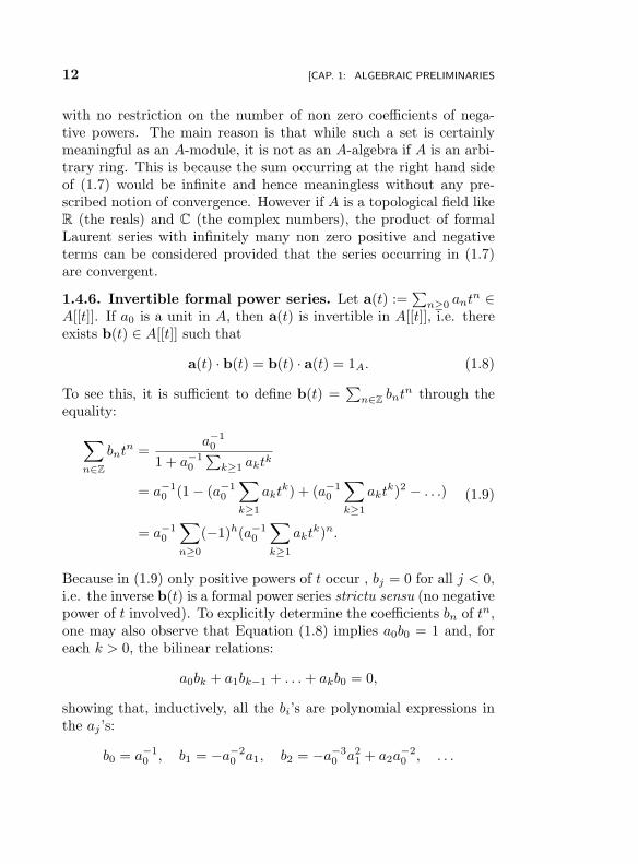
1.4.6. Invertible formal power series. Let a(t) :=∑
n≥0 antn ∈
A[[t]]. If a0 is a unit in A, then a(t) is invertible in A[[t]], i.e. thereexists b(t) ∈ A[[t]] such that
a(t) · b(t) = b(t) · a(t) = 1A. (1.8)
To see this, it is sufficient to define b(t) =∑
n∈Z bntn through the
equality:
∑
n∈Z
bntn =
a−10
1 + a−10
∑k≥1 aktk
= a−10 (1 − (a−1
0
∑
k≥1
aktk) + (a−1
0
∑
k≥1
aktk)2 − . . .)
= a−10
∑
n≥0
(−1)h(a−10
∑
k≥1
aktk)n.
(1.9)
Because in (1.9) only positive powers of t occur , bj = 0 for all j < 0,i.e. the inverse b(t) is a formal power series strictu sensu (no negativepower of t involved). To explicitly determine the coefficients bn of tn,one may also observe that Equation (1.8) implies a0b0 = 1 and, foreach k > 0, the bilinear relations:
a0bk + a1bk−1 + . . .+ akb0 = 0,
showing that, inductively, all the bi’s are polynomial expressions inthe aj ’s:
b0 = a−10 , b1 = −a−2
0 a1, b2 = −a−30 a2
1 + a2a−20 , . . .
“EscoAlgtot˙New”2012/10/10page 13
i
i
i
i
i
i
i
i
[SEC. 1.5: THE FORMAL DERIVATIVE 13
1.5 The formal derivative
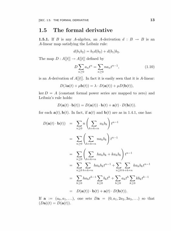
1.5.1. If B is any A-algebra, an A-derivation d : B → B is anA-linear map satisfying the Leibniz rule:
d(b1b2) = b1d(b2) + d(b1)b2.
The map D : A[[t]] → A[[t]] defined by
D∑
n≥0
antn =
∑
n≥0
nantn−1, (1.10)
is an A-derivation of A[[t]]. In fact it is easily seen that it is A-linear:
D(λa(t) + µb(t)) = λ ·D(a(t)) + µD(b(t)),
kerD = A (constant formal power series are mapped to zero) andLeibniz’s rule holds:
D(a(t) · b(t)) = D(a(t)) · b(t) + a(t) ·D(b(t)).
for each a(t),b(t). In fact, if a(t) and b(t) are as in 1.4.1, one has:
D(a(t) · b(t)) =∑
n≥0
n
(∑
h+k=n
ahbk
)tn−1
=∑
n≥0
(∑
h+k=n
nahbk
)tn−1
=∑
n≥0
(∑
h+k=n
hahbk + kahbk
)tn−1
=∑
n≥0
∑
h+k=n
hahbktn−1 +
∑
n≥0
∑
h+k=n
kahbktn−1
=∑
h≥0
hahth−1
∑
k≥0
bktk +
∑
h≥0
ahth∑
k≥0
kbktk−1
= D(a(t)) · b(t) + a(t) ·D(b(t)).
If a := (a0, a1, . . .), one sets Da = (0, a1, 2a2, 3a3, . . .) so that(Da)(t) = D(a(t)).

“EscoAlgtot˙New”2012/10/10page 14
i
i
i
i
i
i
i
i
14 [CAP. 1: ALGEBRAIC PRELIMINARIES
1.5.2. The i-th iteration of the A-derivation D is a differential oper-ator of order i: it is linear as well and satisfies a generalized Leibnizrule whose verification is based on an easy induction:
Dn(a(t) · b(t)) =n∑
k=0
(n
k
)a(k)(t) · b(n−k)(t), (1.11)
where one has set a(i)(t) := Di(a(t)).
1.6 The generating function of binomial
coefficients
1.6.1. To each pair (k, n) of integers one may attach a binomialcoefficient (
n
k
).
By definition, it is the coefficient of tk in the expansion of (1+t)n. Thelatter is a polynomial for n ≥ 0 and a formal power series for n < 0.This is one of the easiest examples where generating functions comeinto play in combinatorics. In fact one can say that f(t) := (1 + t)n
is the generating function of the binomial coefficients:
(1 + t)n =∑
n∈Z
(n
k
),
in the sense that the right hand side of the equality is defined throughits left hand side. In particular
(n
k
)= 0,
for all k < 0, as there is no negative power of t in the expansion of(1 + t)n. Similarly
(0
k
)=
0 if k 6= 0,1 if k = 0,
“EscoAlgtot˙New”2012/10/10page 15
i
i
i
i
i
i
i
i
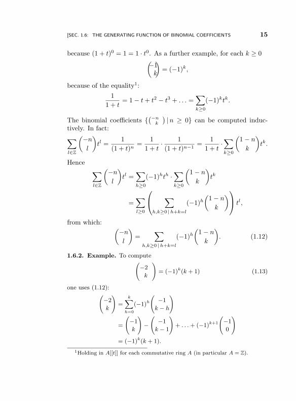
[SEC. 1.6: THE GENERATING FUNCTION OF BINOMIAL COEFFICIENTS 15
because (1 + t)0 = 1 = 1 · t0. As a further example, for each k ≥ 0(−1k
)= (−1)k,
because of the equality1:
1
1 + t= 1 − t+ t2 − t3 + . . . =
∑
k≥0
(−1)ktk.
The binomial coefficients (−n
k
)|n ≥ 0 can be computed induc-
tively. In fact:
∑
l∈Z
(−n
l
)tl =
1
(1 + t)n=
1
1 + t·
1
(1 + t)n−1=
1
1 + t·∑
k≥0
(1 − n
k
)tk.
Hence∑
l∈Z
(−n
l
)tl =
∑
h≥0
(−1)hth ·∑
k≥0
(1 − n
k
)tk
=∑
l≥0
∑
h,k≥0 |h+k=l
(−1)h
(1 − n
k
)
tl,
from which:(−n
l
)=
∑
h,k≥0 |h+k=l
(−1)h
(1 − n
k
). (1.12)
1.6.2. Example. To compute(−2
k
)= (−1)k(k + 1) (1.13)
one uses (1.12):(−2
k
)=
k∑
h=0
(−1)h
(−1
k − h
)
=
(−1
k
)−(
−1
k − 1
)+ . . .+ (−1)k+1
(−1
0
)
= (−1)k(k + 1).
1Holding in A[[t]] for each commutative ring A (in particular A = Z).

“EscoAlgtot˙New”2012/10/10page 16
i
i
i
i
i
i
i
i
16 [CAP. 1: ALGEBRAIC PRELIMINARIES
Formula (1.13) is equivalent to the equality:
1
(1 + t)2= 1 − 2t+ 3t2 − 4t3 + . . .
1.6.3. Example. To compute the coefficient of t3 in (1 + t)−4, one canuse induction as follows:
(−4
3
)=
(−3
3
)−(−3
2
)+
(−3
1
)−(−3
0
)
Now:
(−3
3
)=
(−2
3
)−(−2
2
)+
(−2
1
)−(−2
0
)= −4 − 3 − 2 − 1 = −10;
(−3
2
)=
(−2
2
)−(−2
1
)+
(−2
0
)= 3 + 2 + 1 = 6;
(−3
1
)=
(−2
1
)−(−2
0
)= −2 − 1 = −3.
Therefore (−4
3
)= −10 − 6 − 3 − 1 = −20.
1.6.4. Similarly, for each n > 0, the right hand side of the equality
∑
k∈Z
(n
k
)tk = (1 + t)n = (1 + t) · (1 + t)n−1 = (1 + t) ·
n−1∑
k=0
(n− 1
k
)tk,
can be rewritten as
(1 + t) ·n−1∑
k=0
(n− 1
k
)tk =
n−1∑
k=0
(n− 1
k
)tk +
n−1∑
k=0
(n− 1
k
)tk+1.
But:n−1∑
k=0
(n− 1
k
)tk =
n∑
k=0
(n− 1
k
)tk,
“EscoAlgtot˙New”2012/10/10page 17
i
i
i
i
i
i
i
i
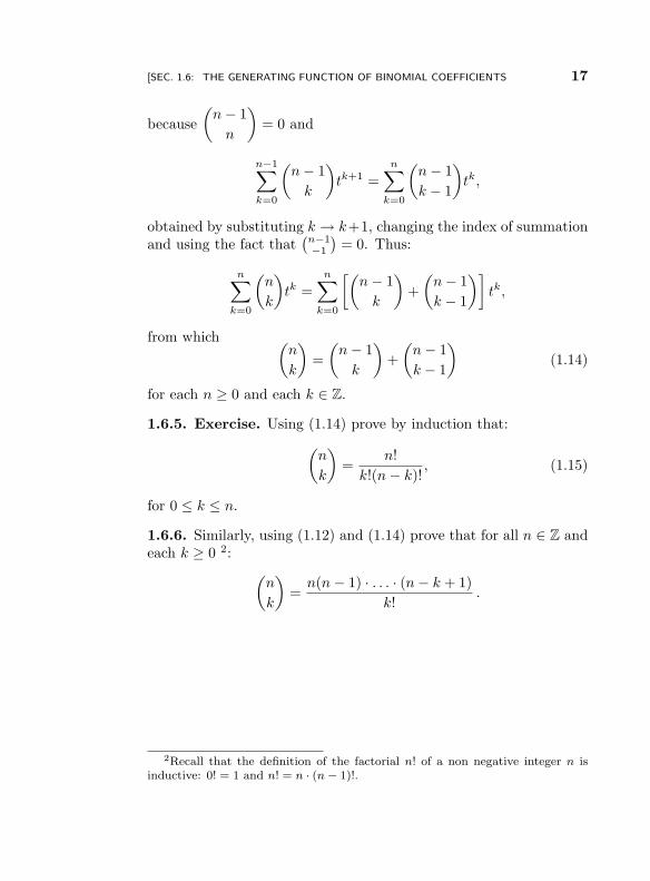
[SEC. 1.6: THE GENERATING FUNCTION OF BINOMIAL COEFFICIENTS 17
because
(n− 1
n
)= 0 and
n−1∑
k=0
(n− 1
k
)tk+1 =
n∑
k=0
(n− 1
k − 1
)tk,
obtained by substituting k → k+1, changing the index of summationand using the fact that
(n−1−1
)= 0. Thus:
n∑
k=0
(n
k
)tk =
n∑
k=0
[(n− 1
k
)+
(n− 1
k − 1
)]tk,
from which (n
k
)=
(n− 1
k
)+
(n− 1
k − 1
)(1.14)
for each n ≥ 0 and each k ∈ Z.
1.6.5. Exercise. Using (1.14) prove by induction that:
(n
k
)=
n!
k!(n− k)!, (1.15)
for 0 ≤ k ≤ n.
1.6.6. Similarly, using (1.12) and (1.14) prove that for all n ∈ Z andeach k ≥ 0 2:
(n
k
)=n(n− 1) · . . . · (n− k + 1)
k!.
2Recall that the definition of the factorial n! of a non negative integer n isinductive: 0! = 1 and n! = n · (n − 1)!.
“EscoAlgtot˙New”2012/10/10page 18
i
i
i
i
i
i
i
i
Chapter 2
Formal power series
over Q-algebras
2.1 Basics on Q-algebras
2.1.1. An associative commutative Q-algebra with unit (Cf. Sec-tion 1.2.1) is a Q-vector space A equipped with a binary operation“ · ” , such that (A,+, ·) is a commutative ring whose product has aneutral element. All overfields of Q, in particular Q, R and C (therationals, the real and the complex numbers), are Q-algebras. A ringof polynomials with coefficients in a Q-algebra is a Q-algebra. Theexpression Q-algebra with no additional adjective will always meanan associative commutative Q-algebra with unit.
2.1.2. A monic polynomial P ∈ A[t] of degree r+ 1 with coefficientsin any Q-algebra A, will be written as:
P (t) := tr+1 − e1(P )tr + . . .+ (−1)r+1er+1(P ),
and the sequence e(P ) = (e1(P ), e2(P ), . . . , er+1(P )) will be said,abusing terminology, the sequence of the coefficients of P .
2.1.3. Example. Suppose that A := Q[x1, . . . , xr+1], where xi is an
18
“EscoAlgtot˙New”2012/10/10page 19
i
i
i
i
i
i
i
i
[SEC. 2.2: FORMAL POWER SERIES IN Q-ALGEBRAS 19
indeterminate over Q (1 ≤ i ≤ r + 1). If
P :=
r+1∏
i=1
(t− xi) = (t− x1) · . . . · (t− xr) · (t− xr+1)
then ei(P ) is the i-th elementary symmetric polynomial in the indetermi-nates x1, . . . , xr, xr+1:
e1(P ) = x1 + . . .+ xr + xr+1,
e2(P ) =∑
1≤i<j≤r+1
xixj ,
...
ej(P ) =∑
1≤i1<i2<...<ij≤r+1
xi1 · . . . · xij
...
er+1(P ) = x1 · . . . · xrxr+1.
This explains the notation, which follows that of [29, p. 12].
2.2 Formal power series in Q-algebras
2.2.1. Since the elements of a Q-algebra A can be multiplied byrational numbers, any formal power series a(t) ∈ A[[t]] can be alter-natively written as an infinite linear combination of the monomialstn
n!:
a(t) =∑
n≥0
an
tn
n!, (an ∈ A)1. (2.1)
The formal Laplace transform (Cf. Section 1.4.2) of a(t) ∈ A[[t]] writ-ten like in (2.1) is
L(a(t)) =∑
n≥0
antn,
1The coefficients an occurring in this expression have not the same meaningof those occurring in (1.4)
“EscoAlgtot˙New”2012/10/10page 20
i
i
i
i
i
i
i
i
20 [CAP. 2: FORMAL POWER SERIES OVER Q-ALGEBRAS
and so L(a) = (a0, a1, . . .). Notice that L is now invertible:
L−1(∑
n≥0
antn) =
∑
n≥0
an
tn
n!,
because it is possible to divide by n!. To each sequence L(a) :=(a0, a1, . . .) in the Q-algebra A corresponds the formal power seriesa(t) as in (2.1). If L(b) := (b0, b1, . . .), the product a(t)b(t) can benow expressed as:
a(t)b(t) =∑
n≥0
[n∑
h=0
(n
h
)ahbn−h
]tn
n!.
In fact
a(t)b(t) =∑
n≥0
an
tn
n!·∑
n≥0
bntn
n!=∑
n≥0
[n−k∑
k=0
ak
k!·
bn−k
(n− k)!
]tn
=∑
n≥0
[n∑
k=0
n! ·ak
k!·
bn−k
(n− k)!
]tn
n!
=∑
n≥0
[n∑
k=0
(n
k
)· ak · bn−k
]tn
n!. (2.2)
The formulas above in particular show that L(a(t)b(t)) 6= L(a(t))×L(b(t)).
2.2.2. Example. For each a ∈ A, the exponential formal power series is
exp(at) =∑
n≥0
an t
n
n!.
For each choice a, b ∈ A, one has:
exp(at) exp(bt)=∑
n≥0
[n∑
h=0
(n
k
)a
kbn−k
]tn
n!=∑
n≥0
(a+ b)n tn
n!= exp((a+ b)t)
The formal Laplace transform of the exponential of at is
L(exp(at)) =∑
n≥0
antn =
1
1 − at.
“EscoAlgtot˙New”2012/10/10page 21
i
i
i
i
i
i
i
i
[SEC. 2.3: POLYNOMIAL Q-ALGEBRAS 21
2.2.3. Example. Let f(t) ∈ C[[t]] be a formal power series with complexcoefficients and let
1
R:= lim
n→∞sup n
√an.
By Hadamard’s Theorem (see e.g. [6, p. 20]), f defines a holomorphic
function in the disc DR := z ∈ C | |z| < R given by f(z) =∑
n≥0
anzn . If
a ∈ C, exp(at) defines the entire (i.e. defined on the whole C) exponentialfunction exp(az).
2.2.4. A map ψ : A → B is a homomorphism of Q-algebras ifψ(λ ·a1 +µ ·a2) = λ ·ψ(a1)+µ ·ψ(a2) and ψ(a1a2) = ψ(a1) ·ψ(a2), forarbitrary choices of λ, µ ∈ Q and a1, a2 ∈ A. If ψ ∈ HomQ−alg(A,B),
then the induced Q-algebra homomorphism ψ : A[[t]] → B[[t]] can beexpressed as:
ψ
∑
n≥0
an
tn
n!
=∑
n≥0
ψ(an
n!
)tn =
∑
n≥0
ψ(an)tn
n!.
2.3 Polynomial Q-algebras
2.3.1. Let us fix once and for all a sequence
e := (e1, e2, . . . , ) (2.3)
of indeterminates over Q. For each r ≥ 0, denote by Er the polyno-mial Q-algebra
Er := Q[e1, e2, . . . , er+1]. (2.4)
We set by convention E−1 = Q. By giving degree i to the indetermi-nate ei, the algebra Er can be seen as a graded Q-algebra:
Er :=⊕
w≥0
(Er)w,
where (Er)w is the set of all weighted homogeneous polynomials ofdegree w. For example
(Er)1 = Q·e1, (Er)2 = Q·e21⊕Q·e2, (Er)3 = Q·e31⊕Q·e1e2⊕Q·e3, . . .
“EscoAlgtot˙New”2012/10/10page 22
i
i
i
i
i
i
i
i
22 [CAP. 2: FORMAL POWER SERIES OVER Q-ALGEBRAS
2.3.2. If −1 ≤ s ≤ r, the module Es may be viewed either as Q-subalgebra of Er or as a quotient of it under the map
pr,s : Er → Es (2.5)
mapping es+1, . . . , er+1 to zero. Notice that pr2,r3pr1,r2
= pr1,r3for
each r1 ≥ r2 ≥ r3 and hence the ring of infinitely many indetermi-nates
E∞ := Q[e1, e2, . . .],
is in fact the inverse (or projective) limit of the algebras Er in thecategory of graded Q-algebras. This just means that if B is any Q-algebra equipped with homomorphism qr : B → Er, then there is aunique Q-algebra homomorphism ψ : B → E∞ such that qr = pr ψ,where
pr : E∞ → Er (2.6)
is the unique Q-algebra epimorphism sending ei 7→ ei if 1 ≤ i ≤ r+ 1and ej 7→ 0 if j > r+ 1. An element P ∈ E∞ is a polynomial P ∈ Er
for some r ≥ −1. In other words E∞ :=⋃
r≥−1Er.
2.3.3. For each 0 ≤ r ≤ ∞, the algebras Er are the most economicalones, in the following sense. Given any other Q-algebra A and an (r+1)-tuple a := (a1, . . . , ar, ar+1) ∈ Ar+1, there is a natural evaluationmorphism
eva : Er −→ A,
P 7→ P (a),(2.7)
which is indeed the unique Q-algebra homomorphism mapping ei 7→ai, for 1 ≤ i ≤ r + 1.
2.3.4. Definition. The universal Q-polynomial Ur+1 ∈ Er[t] ofdegree r + 1 is
Ur+1(t) = tr+1 − e1tr + . . .+ (−1)r+1er+1. (2.8)
In other words ei(Ur+1(t)) = ei. We also define, for each r ≥ 0:
Vr+1 = tr+1Ur+1
(1
t
)= 1 − e1t+ . . .+ (−1)r+1er+1t
r+1. (2.9)
“EscoAlgtot˙New”2012/10/10page 23
i
i
i
i
i
i
i
i
[SEC. 2.3: POLYNOMIAL Q-ALGEBRAS 23
and (setting e0 = 1):
V∞ =∑
n≥0
(−1)nentn = 1 − e1t+ e2t
2 − . . . ∈ E∞[[t]]. (2.10)
Notice that under the maps (2.5) pr,s : Er → Es and (2.6) pr : E∞ →Er, one has pr,s(Vr+1) = Vs+1 and pr(V∞) = Vr+1.
2.3.5. To each sequence L(a) := (a0, a1, . . . , ) of elements of anarbitrary Er-algebra A, one may attach the sequence U0(a), U1(a),U2(a), . . . by setting U0(a) = a0 and
Ui(a) := ai − e1ai−1 + . . .+ (−1)r+1er+1ai−r−1 (2.11)
for each i ≥ 1, with the convention that aj = 0 if j < 0. So, forinstance,
U1(a) = a1 − e1a0, U2(a) = a2 − e1a1 + e2a0, . . .
Any finite sequence in A will be thought of as an infinite sequencesuch that all but finitely many terms are zero.
2.3.6. Remark. For each j ∈ Z, let sj(a) be the sequence a shiftedby j
sj(a) = (aj , aj+1, . . .).
In particular s0(a) = a. If er+1+j = 0 for each j > 0, then
Ur+1+j(a) = Ur+1(sj(a)).
2.3.7. Combinatorial Lemma. For each 0 ≤ r ≤ ∞, the equality∑
j=0
(−1)jejtj∑
n≥0
antn =
∑
i≥0
Ui(a)ti (2.12)
holds in A[[t]].
Proof. By the rule (2.2) for multiplying formal power series, it turnsout that the coefficient of ti, for i ≥ 0, is the sum of products of theform (−1)jejak such that j + k = i, i.e.:
ai − e1ai−1 + . . .+ (−1)ieia0 = Ui(a) (2.13)
and (2.12) is proven.
“EscoAlgtot˙New”2012/10/10page 24
i
i
i
i
i
i
i
i
24 [CAP. 2: FORMAL POWER SERIES OVER Q-ALGEBRAS
2.3.8. Remark. Equations (2.13) for 0 ≤ i ≤ r can be summarizedinto the following equality:
U0(a)U1(a)U2(a)
...Ur(a)
= Er ·
a0
a1
a2
...ar
(2.14)
where
Er := ((−1)i−jei−j)
=
1 0 0 . . . 0−e1 1 0 . . . 0e2 −e1 1 . . . 0...
......
. . ....
(−1)rer (−1)r−1er−1 (−1)r−2er−2 . . . 1
.
2.3.9. Let 0 ≤ s ≤ ∞ and let h = (hj)j∈Z be the sequence ofelements of Es defined through the equality
∑
n∈Z
hntn =
1
Vs+1(t), (2.15)
holding inEs[[t]]. As the inverse of the polynomial Vs+1(t)=s+1∑i=0
(−1)iei
is an A–linear combination of positive powers of t only, then hj = 0for all j < 0. In addition h0 = 1. Equaltion (2.15) is equivalent to:
1 =s+1∑
i=0
(−1)ieiti ·∑
n≥0
hntn =
∑
j≥0
Uj(h)tj , (2.16)
which implies U0(h) = 1 and Uj(h) = 0 for all j ≥ 1. The conditionsU0(h) = 1 and Uj(h) = 0 for each 0 ≤ r < s can be equivalentlywritten as
Er · Hr = Hr · Er = 1, (2.17)
“EscoAlgtot˙New”2012/10/10page 25
i
i
i
i
i
i
i
i
[SEC. 2.3: POLYNOMIAL Q-ALGEBRAS 25
where 1 denotes the (r + 1) × (r + 1) identity matrix and
Hr := (hi−j) =
1 0 0 . . . 0h1 1 0 . . . 0h2 h1 1 . . . 0...
......
. . ....
hr hr−1 hr−2 . . . 1
.
In particular, Equation (2.14) can be written as:
a0
a1
...ar
= Hr ·
U0(a)U1(a)
...Ur(a)
. (2.18)
2.3.10. For each j ∈ Z, let
u(j) = L−1(sj(h)(t)) =∑
n≥0
hn+j
tn
n!. (2.19)
Notice that Diu(j) = u(i+j), for all i, j ∈ Z. Then:
2.3.11. Main Lemma. If A is any Er-algebra and L(a(t)) =∑n≥0 ant
n ∈ A[[t]], then the formal power series u(j) are linearlyindependent in A[[t]] and, in addition:
a(t) =∑
j≥0
an
tn
n!=∑
n≥0
Uj(a)u(−j) = a0u(0)+U1(a)u(−1)+ . . . (2.20)
Lemma 2.3.11 says that each element of A[[t]] is an infinite linearcombination of the u(−j). Taking infinite linear combinations of theu(−j) is meaningful, as the sequence (u(−j))j≥0 is summable in thesense of [6, p. 11]: for each k ≥ 0, all terms except a finite numberhave order greater that k (the order of a formal power series is thesmallest power of t occurring in it).
“EscoAlgtot˙New”2012/10/10page 26
i
i
i
i
i
i
i
i
26 [CAP. 2: FORMAL POWER SERIES OVER Q-ALGEBRAS
Proof of Lemma 2.3.11. For each j ≥ 0, the order of u(−j) is j:
u(−j) =tj
j!+∑
n≥1
hn
tj+n
(j + n)!.
Hence all the u(−j) are linearly independent, because they have dis-tinct orders. To prove (2.20) one considers the coefficient of tn in theright hand side of it:
∑
j≥0
Uj(a)u(−j)
n
=∑
j≥0
Uj(a)[u(−j)(0)]n =∑
j≥0
Uj(a)hn−j
= U0(a)hn + hn−1U1(a) + . . .+ h0Un(a) = an
where [ ]n denotes the coefficient of degree n and the last equality isdue to (2.18).
2.3.12. Example. For each n ≥ 0 one has
tn = u
(−n) − e1u(−n−1) + e2u
(−n−2) + . . .
Furthermore
eat = u
(0) + U1(a)u(−1) + U2(a)u
(−2) + . . .
2.3.13. The map (2.7) induces a Q-algebra homomorphism eva :Er[t] → A[t], denoted in the same way abusing notation:
tr+1 − p1(ei)tr + . . .+ (−1)r+1pr+1(ei) 7→ tr+1 − p1(ai)t
r
+ . . .+ (−1)r+1pr+1(ai),
where p1, . . . , pr+1 are arbitrary elements in Er. The adjective uni-versal used in Definition 2.3.4 is to emphasize the fact that for eachmonic P ∈ A[t] of degree r + 1, the unique evaluation morphismev
e(P ) mapping ei 7→ ei(P ), sends Ur+1 to P :
eve(P )(Ur+1(t)) = P (t).
“EscoAlgtot˙New”2012/10/10page 27
i
i
i
i
i
i
i
i
Chapter 3
Universal Solutions to
Linear ODEs
In this chapter A will denote any Er-algebra, fixed once and for all.
3.1 Universal Linear Homogeneous ODE
3.1.1. The Er-algebra A is a Q-algebra as well. Thus, formal powerseries in A[[t]] will be written as in (2.1) and D : A[[t]] → A[[t]], thefirst–order ordinary differential operator (1.10), in the form
(Da)(t) := D
∑
n≥0
an
tn
n!
=∑
n≥0
an+1tn
n!.
For each i ∈ Z, let:
(Dia)(t) := Di
∑
n≥0
an
tn
n!
=∑
n≥0
an+i
tn
n!, (3.1)
with the convention that aj = 0 if j < 0. In particular D0 = idA[[t]]
is the identity morphism of A[[t]] and, if i ≥ 0, the operator Di isjust the i-th iteration of the endomorphism D.
27
“EscoAlgtot˙New”2012/10/10page 28
i
i
i
i
i
i
i
i
28 [CAP. 3: UNIVERSAL SOLUTIONS TO LINEAR ODES
3.1.2. For a(t) ∈ A[[t]] and n ≥ 0, denote by (Dna)(0) the class ofDna(t) modulo the ideal (tn+1), so that:
(Dna)(0) = an.
Any formal power series a(t) ∈ A[[t]] can be expressed in Taylor form:
a(t) =∑
n≥0
(Dna)(0)tn
n!.
One says that a(t) vanishes at 0 with multiplicity at least n + 1 ifa(t) ∈ (tn+1) or, equivalently, if (Dja)(0) = 0 for all 0 ≤ j ≤ n. Foreach integer r ≥ 0, the map
A[[t]] −→A[[t]]
(tr+1)
associates to each formal power series a(t) like (2.1) its truncation tothe power tr:
a(t) 7→ a0 + a1t+ . . .+ ar
tr
r!∈ A[t].
3.1.3. By Universal differential operator we shall mean the evalua-tion at D of the universal monic polynomial (2.8):
Ur+1(D) := Dr+1−e1Dr + . . .+(−1)r+1er+1 ∈ EndQ(Er[[t]]). (3.2)
LetUr := kerUr+1(D).
It is an Er-submodule of Er[[t]]. Then
Ur ⊗ErA := ker(Ur+1(D) ⊗A 1A)
is the A-submodule of A[[t]] of solutions of the universal ODE:
Ur+1(D)y = y(r+1) − e1y(r) + . . .+ (−1)r+1er+1y = 0. (3.3)
In general, if
f :=∑
n≥0
fn
tn
n!∈ A[[t]], (3.4)
“EscoAlgtot˙New”2012/10/10page 29
i
i
i
i
i
i
i
i
[SEC. 3.1: UNIVERSAL LINEAR HOMOGENEOUS ODE 29
then a solution of the linear Ordinary Differential Equation (ODE)
Ur+1(D)y = f (3.5)
is an element of the set Ur+1(D)−1(f) ⊆ A[[t]].
3.1.4. The linear ODE (3.5) is usually more explicitly written as:
Dr+1y − e1Dry + . . .+ (−1)r+1er+1y = f . (3.6)
If f is the zero formal power series, then Ur+1(D)−1(0) = Ur ⊗A is asubmodule of A[[t]] called the module of solutions of the homogeneouslinear ODE P (D)y = 0.
3.1.5. Proposition. Let y0(t) ∈ Ur+1(D)−1(f). Then
Ur+1(D)−1(f) = y0(t) + kerUr+1(D)
= y0(t) + y(t) | y(t) ∈ kerUr+1(D).
Proof. It is standard linear algebra. The A-linearity of Ur+1(D) im-plies the inclusion y0(t) + kerUr+1(D) ⊆ Ur+1(D)−1(f). Conversely,if y1(t) ∈ Ur+1(D)−1(f), then y1(t) − y0(t) ∈ kerUr+1(D), and thenUr+1(D)−1(f) ⊆ y0(t) + kerUr+1(D).
3.1.6. Proposition. Let a(t) ∈ A[[t]] as in (2.1). Then a(t) ∈kerUr+1(D) if and only the bilinear relation:
Un+r+1(a) := an+r+1 − e1an+r + . . .+ (−1)r+1er+1an = 0 (3.7)
holds for all n ≥ 0.Proof. Substituting y = a(t) in the equation (3.6) with f = 0 andkeeping into account the expression of Di given by (3.1), one obtains:
∑
n≥0
an+r+1tn
n!− e1
∑
n≥0
an+r
tn
n!+ . . .+ (−1)r+1er+1
∑
n≥0
an
tn
n!=
=∑
n≥0
(an+r+1 − e1an+r + . . .+ (−1)r+1er+1an
) tn
n!. (3.8)
Then a(t) ∈ kerUr+1(D) if the formal power series (3.8) vanishes, i.e.if and only if (3.7) holds for all n ≥ 0.

“EscoAlgtot˙New”2012/10/10page 30
i
i
i
i
i
i
i
i
30 [CAP. 3: UNIVERSAL SOLUTIONS TO LINEAR ODES
3.1.7. Example. The formal power series exp(e1t) solves the differentialequation U1(D)y = 0. In fact
en+11 − e1 · en
1 = en+11 − e1 · λen
1 = en+11 − e
n+11 = 0.
If A is any Q-algebra and a ∈ A, then A has a structure of algebra overE0 := Q[e1] via the unique homomorphism mapping e1 7→ a. The modulestructure is given by e1 · 1A = a. Hence exp(at) ∈ A[[t]] can be seen as asolution of the equation Dy − e1y = 0 as well. In fact
an+1 − e1 · an = a
n+1 − a · an = an+1 − a
n+1 = 0.
which is the same as saying that exp(at) is solution of the differentialequation Dy − ay = 0. The equality
P (t) := t− a = U1(t) ⊗ 1A,
implies
kerP (D)= kerU1(D)⊗E1 A= ker(D−a)=[exp(at)] := λ ·exp(at) |λ ∈ A.
3.1.8. Example. Suppose that P ∈ A[t] is monic of degree r+ 1 and hasa root in A, i.e. there exists a ∈ A such that P (a) = 0. It turns out thatexp(at) is a solution of P (D)y = 0. In fact, by Ruffini’s theorem, P (t)admits the decomposition
P (t) = Q(t)(t− a),
where Q(t) is a monic polynomial of degree r. It follows that
P (D) exp(at) = Q(D)(D − a)(exp(at)) = 0
because exp(at) ∈ ker(D − a) by Example 3.1.7.
3.1.9. When imposing a formal power series a(t) to belong tokerUr+1(D), no condition is required on the first r + 1 coefficientsa0, a1, . . . , ar: these are the initial conditions of the solution: aj =(Dja)(0), for 0 ≤ j ≤ r.
3.1.10. Proposition. If all the initial conditions a0, a1, . . . , ar ofa(t) ∈ kerUr+1(D) vanish, then a(t) = 0, i.e. an = 0 for each n ≥ 0.
Proof. In fact if a(t) is a solution, equation (3.7) holds for all n ≥ 0.In particular, for n = 0, it gives ar+1 = 0 and by induction, assumingthat a0 = a1 = . . . = ar+k−1 = 0, one proves that ar+k = 0, byusing (3.7) again.
“EscoAlgtot˙New”2012/10/10page 31
i
i
i
i
i
i
i
i
[SEC. 3.2: UNIVERSAL SOLUTIONS 31
3.1.11. Corollary. Two formal power series a(t),b(t)∈ kerUr+1(D)coincide if and only if they have the same initial conditions.
Proof. If a(t) = b(t), the initial conditions obviously coincide.Conversely, if they have the same initial conditions a(t) − b(t) ∈kerUr+1(D) and all initial conditions vanish, then a(t) − b(t) = 0,because of 3.1.10, i.e. a(t) = b(t).
As in Section 2.3 let now h = (h0, h1, . . .) be given by
∑
n∈Z
hntn =
1
1 − e1t+ . . .+ (−1)r+1er+1tr+1
and the (u(j))j∈Z as in (2.19).
3.2 Universal solutions
3.2.1. Theorem. The A-module Ur ⊗A := kerUr+1(D) ⊗A is freeof rank r + 1 generated by
(u(0), u(−1), . . . , u(−r)). (3.9)
Proof. We already know that (u(−j))j≥0 are linearly independent inA[[t]]. In addition, for all 0 ≤ j ≤ r one has:
Ur+1(D)u(−j) = Ur+1(D)Dr−ju(−r) = Dr−jUr+1(D)u(−r),
and then to show that u(−j) ∈ Ur for 0 ≤ j ≤ r, it suffices to showthat u(−r) ∈ Ur. Now
L(u(−r)) = s−r(h) = (0 . . . , 0︸ ︷︷ ︸r times
, 1, h1, . . .)
(recall that hj = 0 if j < 0). The left–hand side of Equation (3.7)with an = hn−r is:
an+r+1−e1an+r + . . .+ (−1)r+1er+1an
= hn+1 − e1hn + . . .+ (−1)r+1er+1hn−r,(3.10)
and the right–hand side of (3.10) is Un+1(h), the coefficient of tn+1 inexpansion (2.16), which vanishes for all n ≥ 0 by definition of the hi.

“EscoAlgtot˙New”2012/10/10page 32
i
i
i
i
i
i
i
i
32 [CAP. 3: UNIVERSAL SOLUTIONS TO LINEAR ODES
By criterion 3.1.6, u(−r) ∈ Ur, and then u(−j) ∈ Ur for all 0 ≤ j ≤ r.To show that (u(0), . . . , u(−r)) generates Ur over A, recall that each
a(t) =∑
n≥0
an
tn
n!∈ A[[t]]
can be expressed as an infinite linear combination of the (u(−j))j≥0:
a(t) = U0(a)u(0) + U1(a)u(−1) + . . .+ Ur(a)u(−r)
+∑
n≥0
Ur+1+n(a)tr+1+n,
by (2.3.11). But a(t) ∈ kerUr if and only if Ur+1+n(a) = 0 for eachn ≥ 0, by Proposition 3.1.6, i.e. if and only if
a(t) = U0(a)u(0) + . . .+ Ur(a)u(−r) , (3.11)
and the theorem is proven.
Formula (3.11) will be called the Universal Cauchy Formula.
3.2.2. Remark. Notice that (u(0), u(−1), . . . , u(−r)) is a basis ofkerUr+1(D) such that each u(−j) is obtained by differentiating r − jtimes the solution u(−r). Such kinds of bases are known in analysis.In particular u(−r) generates the impulsive response kernel. See e.g.the nice account [5] by Camporesi.
3.2.3. Example. The universal Cauchy formula says that the mapA[D] → Ur defined as the A-linear extension of Dj 7→ Dju(−r) =u(j−r) is an epimorphism. In fact any element of kerUr+1(D) ⊗A can be written uniquely as an A–linear combination of u(−j) =Dr−ju(−r), for 0 ≤ j ≤ r. The kernel is generated by the polynomialexpression in D vanishing on Ur, which is precisely Ur+1(D). So, oneobtains the A-algebra isomorphism:
kerUr+1(D) ∼=A[D]
(kerUr+1(D) ⊗A).
“EscoAlgtot˙New”2012/10/10page 33
i
i
i
i
i
i
i
i
[SEC. 3.2: UNIVERSAL SOLUTIONS 33
The latter is an A-algebra generated by the differential operator D.It is a D-module, i.e. a module generated by differential operators,see [9] for a nice and enlightening exposition. Much of the theory wehave presented could be developed using solely this language, but wewill not pursue this alternative approach just for reasons of space.Notice that
A[D]
(kerUr+1(D) ⊗A)=
Er[D]
kerUr+1(D)⊗Er
A
and so the right–hand side is the universal D-module associated tothe differential operator D. It is a free Er-module of rank r + 1generated by 1,D, . . . ,Dr.
3.2.4. As suggested by Example 3.1.7, if A is any Q-algebra and P ∈A[T ] is any monic polynomial of degree r + 1, the unique Q-algebrahomomorphism ψP : Er → A mapping ei 7→ ei(P ), for 1 ≤ i ≤ r+ 1,makes A into an Er-algebra. Then (3.11) holds as well in such asituation. In particular, by definition of the Er-algebra structure ofA, eja = ψP (ej)a = ej(P )a, for each a ∈ A, and then the Er-moduleproduct Ur+1(D)y is the same as P (D)y ∈ A[[t]] in this case. Itfollows that a(t) is a solution of the equation P (D)y = 0 if and onlyif it is a solution of Ur+1(D)y = 0, thinking of y as an element of theEr-algebra A[[t]]. We have then proven the following:
3.2.5. Theorem. Given P (D)y = 0, a homogeneous linear ODEwith coefficients in any Q-algebra A, then
kerP (D) = kerUr+1(D) ⊗ErA,
where the tensor product is taken with respect to the Er-algebra struc-ture inherited by A via the unique homomorphism ψP : Er → Amapping ei 7→ ei(P ).
Theorem 3.2.5 can be rephrased by saying that (u(0), u(−1), . . . ,u(−r)) is a universal basis of solutions, i.e. that each solution ofP (D)y = 0 is an A-linear combination of the image of the universal
basis of Ur under ψP .
3.2.6. Example. Let A := Q[x1, x2] where x1, x2 are indeterminates, andconsider the E1-algebra structure determined by the map E1 → A given
“EscoAlgtot˙New”2012/10/10page 34
i
i
i
i
i
i
i
i
34 [CAP. 3: UNIVERSAL SOLUTIONS TO LINEAR ODES
by e1 7→ x1 + x2 and e2 7→ x1x2. Then (exp(x1t) and exp(x2t) are linearlyindependent solutions of U2(D)y = 0. However, they are not a basis ofkerU2(D). In fact, by the universal Cauchy formula (3.11):
exp(x1t) = u(0) − x2u(−1),
exp(x2t) = u(0) − x1u(−1)
from which, e.g.:
(x1 − x2)u(−1) = exp(x1t) − exp(x2t).
It follows that u(−1) cannot be expressed as linear combination of exp(x1t)and exp(x2t), because x1 − x2 is not invertible in A. Clearly (exp(x1t),exp(x2t)) is a basis of ker(U2) thought of as a submodule of A(x1−x2)[[t]],where A(x1−x2) denotes localization at the multiplicative set 1, x1 − x2,
(x1 − x2)2, . . .). This example shows that u(0) and u(−1) is a “proper”
canonical basis of kerU2(D).
3.2.7. Example. Consider the differential equation y′′ + y = 0, thoughtof linear ODE with real (or even rational) coefficients. This is the same asP (D)y = 0 where P (t) = t2 +1. The above theorem says that all solutionsare of the form
λu(0) + µu
(1) = λ · ψP (u(0)) + µ · ψP (u(−1)), (λ, µ ∈ R)
where the linear combination is taken with respect to the unique E1-modulestructure of R induced by the unique Q-algebra homomorphism sendinge1 7→ 0 and e2 7→ 1. Let v(i) = ψP (u(i)). First of all notice that
1
ψP (V2(t))=
1
1 + t2= 1 − t
2 + t4 − . . .
According to the recipe of theTheorem, then,
v(0) = 1 − t2
2!+t4
4!− . . .
and v(−1) is the unique primitive of v(0) vanishing at 0, i.e.:
v(−1) = t− t3
3!+t5
5!− . . . ,
Both series have convergence radius equal to ∞ and they define in factanalytic functions everywhere on R, the well known sine and cosine.
“EscoAlgtot˙New”2012/10/10page 35
i
i
i
i
i
i
i
i
[SEC. 3.2: UNIVERSAL SOLUTIONS 35
3.2.8. Example: the universal Euler formula. Let U2(t) = t2 −e1t+ e2 ∈ E1[t]. The polynomial U2(t) has no roots in E1[t] but one mayconstruct a larger Q-algebra where U2 splits as the product of two linearfactors. The most economical one is the universal splitting algebra of U2(t)(see [10]) , constructed as follows. Let
E1[x] :=E1[t]
(U2(t))
where x denotes the class of t modulo the principal ideal generated byU1(t). Then
U1(x) = 0,
by construction, and so x is a root of the polynomial U1(t) ∈ E1[x][t].Indeed
U1(t) = (t− x)(t− (e1 − x)),
in E1[x][t]. Clearly E1[x] is an E1-algebra and exp(xt) is an element ofkerU1(D). By the universal Cauchy formula (3.11):
exp(xt) = u(0) + (x− e1)u(−1) , (3.12)
because the initial conditions of exp(xt) are 1 and x. It is reasonable to callEquation (3.12) universal Euler formula. In fact, consider the differentialequation
y′′ + y = 0,
with coefficients in the Q-algebra C. Then i :=√−1 is a root of the charac-
teristic polynomial t2 +1 of the equation. Therefore exp(it) ∈ ker(D2 +1),i.e.
exp(it) = v(0) + (i− e1)v
(−1)
under the E1-algebra structure of C induced by the unique homomorphismψ : E1 → C sending e1 7→ 0 and e2 7→ 1, where we have defined vi = ψ(ui).One has then:
exp(it) = v(0) + iv
(−1) ∈ ker(D2 + 1) ⊆ C[[t]].
i.e.exp(it) = cos t+ i sin t, (3.13)
by Example 3.2.7.
3.2.9. Example. The Euler formula (3.13) generalizes as follows. Ifv(0), v(−1), . . . , v(−r) are the canonical solutions of the equation yr+1+y = 0and if x is any (r + 1)th root of unity, then
exp(xt) = u(0) + xu
(−1) + . . .+ xru
(−r).
“EscoAlgtot˙New”2012/10/10page 36
i
i
i
i
i
i
i
i
36 [CAP. 3: UNIVERSAL SOLUTIONS TO LINEAR ODES
3.3 A few remarks on the formal Laplace
transform
3.3.1. Recall that the formal Laplace transform L : A[[t]] → A[[t]] isdefined by L(tn) = n!tn and extends to infinite linear combinationsof powers of t, i.e.:
L
∑
n≥0
an
tn
n!
=∑
n≥0
an
L(tn)
n!=∑
n≥0
antn.
3.3.2. Proposition. For each h ≥ −1 and each a(t) ∈ A[[t]] onehas:
th+1L(D(h+1)a)(t) = L(a)(t) − a0 − a1t− . . .− ahth. (3.14)
Proof. If L(a) = (a0, a1, a2, . . .), then
th+1L(Dh+1a)(t) = th+1L
∑
n≥0
an+h+1tn
n!
= th+1∑
n≥0
an+h+1tn
=∑
n≥0
an+h+1tn+h+1
=∑
n≥0
antn − a0 − a1t− . . .− aht
h
= L(a)(t) − a0 − a1t− . . .− ahth.
3.3.3. Classically, the Laplace transform is defined for real functionsf : R → R of one real variable. Even if the domain of f coincideswith the entire real line, the Laplace transform
L(f(t))(s) =
∫ ∞
0
exp(−st)f(t)dt (3.15)
“EscoAlgtot˙New”2012/10/10page 37
i
i
i
i
i
i
i
i
[SEC. 3.3: A FEW REMARKS ON THE FORMAL LAPLACE TRANSFORM 37
may be not, because of the restriction on the parameter s to guaran-tee the convergence of the integral (3.15). For intance, the Laplacetransform of f(t) = exp(at) is, according to (3.15), (s − a)−1, butthis is defined only for s > a, otherwise the integral
∫ ∞
0
exp((a− s)t)dt
would not converge. The integral (3.15) is defined for analytic func-tions as well, and then it commutes with infinite sums. For analyticfunctions it is completely determined by the action on monomials tn:
L(tn)(s) =
∫ ∞
0
exp(−st)tndt =n!
sn+1
Therefore on analytic functions we have the equation:
L(f)(s) =1
s· L(f)
(1
s
)(3.16)
and, conversely
L(f) =1
tL(f)
(1
t
)(3.17)
If one considers the Laplace transform as acting on elements of R[[t]],equations (3.16) and (3.17) tell us that the pair (L,L) is the localrepresentation of a rational section of the tautological bundle T overthe real projective line RP1, which is the Mobius band. The sectionL(tn) : RP1 → T is given as follows
(x0, x1) 7→ L(tn)(x0 : x1) = n!xn
0
xn+11
and extended by linearity to infinite sums. It is clearly not defined atthe point (1 : 0). Furthermore it is not a function, because it dependson the representative used to represent a point P := (x0 : x1). Onthe open set D0 := (x0 : x1) |x0 6= 0 ⊆ RP1 it is represented by
L(tn)(x0 : x1) =n!
sn+1
“EscoAlgtot˙New”2012/10/10page 38
i
i
i
i
i
i
i
i
38 [CAP. 3: UNIVERSAL SOLUTIONS TO LINEAR ODES
where we set s := x0/x1, while on the open set D1 := (x1 : x0) |x1 6=0 it takes the form
L(tn)(x0 : x1) = n!tn
where t = x1/x0. The two “versions” of the Laplace transform maybe viewed, at least for analytic functions, as two different local rep-resentations of a same rational section of the tautological bundle.Working over the complex numbers, one can say that the Laplacetransform L(f) of a holomorphic function on the complex plane is ameromorphic section of the line bundle OP1(−1), which correspondsto a divisor of degree −1 on the projective line.
3.4 Linear ODEs with source
The best way to study non–homogeneous linear ODEs is via the for-mal Laplace transform tn 7→ n!tn. See below.
3.4.1. Let L(f) = (f0, f1, . . .) and L(c) = (c0, c1, . . . , cr) be twosequences of indeterminates over Er. Let Fr := Er[c, f ]. From theinfinite sequence L(f) form
f(t) =∑
n≥0
fn
tn
n!∈ Fr[[t]].
Solving the universal Cauchy problem
Ur+1(D)y = f ,
(Diy)(0) = ci, 0 ≤ i ≤ r,(3.18)
amounts to finding a formal power series p ∈ Ur+1(D)−1(f) havingL(c) as a vector of initial conditions. The first of (3.18) implies theequality:
tr+1L(Ur+1(D)y) = tr+1L(f), (r ≥ 0)
from which
tr+1(L(y(r+1))− e1L(y(r)) + . . .+ (−1)r+1er+1L(y)) =∑
n≥0
fntn+r+1,
“EscoAlgtot˙New”2012/10/10page 39
i
i
i
i
i
i
i
i
[SEC. 3.4: LINEAR ODES WITH SOURCE 39
i.e., applying Proposition 3.3.2:
L(y) −r∑
i=0
citi−e1t
(L(y) −
r−1∑
i=0
citi
)+ . . .+ (−1)r+1tr+1L(y)
=∑
n≥0
fntn+r+1.
Factorizing L(y) and a few more easy computations yield:
L(y)(1 − e1t+ . . .+ (−1)r+1er+1tr+1)
= U0(c) + U1(c)t+ . . .+ Ur(c)tr +∑
n≥0
fntn+r+1.
One eventually gets the expression:
L(y) = L(p(t)),
where
L(p(t)) =U0(c) + U1(c)t+ . . .+ Ur(c)tr +
∑n≥r+1 fn−r−1t
n
1 − e1t+ . . .+ (−1)r+1er+1tr+1.
(3.19)
Writing L(p(t)) as∑
n≥0 pntn, with pn determined by equality (3.19)
holding in Fr[[t]], then
p(t) =∑
n≥0
pn
tn
n!
is the unique solution of the Cauchy problem (3.18 ).
3.4.2. Corollary. The formal Laplace transform of u(−j) for 0 ≤j ≤ r is:
L(u(−j)) =tj
1 − e1t+ . . .+ (−1)r+1er+1tr+1= tj
∑
n≥0
hntn.
“EscoAlgtot˙New”2012/10/10page 40
i
i
i
i
i
i
i
i
40 [CAP. 3: UNIVERSAL SOLUTIONS TO LINEAR ODES
3.4.3. Remark. If r < ∞, a formal power series a(t) is a solutionof Ur+1(D)y = 0 if and only if (Cf. (2.9)):
L(a(t)) =1
Vr+1(t), (3.20)
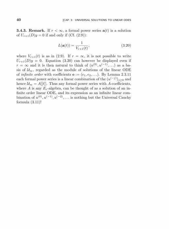
where Vr+1(t) is as in (2.9). If r = ∞, it is not possible to writeUr+1(D)y = 0. Equation (3.20) can however be displayed even ifr = ∞ and it is then natural to think of (u(0), u(−1), . . .) as a ba-sis of U∞, regarded as the module of solutions of the linear ODEof infinite order with coefficients e := (e1, e2, . . .). By Lemma 2.3.11each formal power series is a linear combination of the (u(−j))j≥0 andhence U∞ = A[[t]]. Thus any formal power series with A-coefficients,where A is any Er-algebra, can be thought of as a solution of an in-finite order linear ODE, and its expression as an infinite linear com-bination of u(0), u(−1), u(−2), . . . is nothing but the Universal Cauchyformula (3.11)!
“EscoAlgtot˙New”2012/10/10page 41
i
i
i
i
i
i
i
i
Chapter 4
Generalized Wronskians
4.1 Partitions
4.1.1. By a partition of length at most r + 1 one will mean a non–increasing sequence λ = (λ0 ≥ λ1 ≥ . . . ≥ λr) of non negative inte-gers. Each λi is said to be a part of the partition. The length ℓ(λ) isthe number of its non zero parts and its weight is |λ| =
∑ri=0 λi. Each
partition is a partition of the integer |λ|. The set of all partitions oflength ≤ r+ 1 will be denoted by ℓr. If λ, µ ∈ ℓr, the partition λ+µis the partition whose parts are the sum of the parts
λ+ µ = (λ0 + µ0, λ1 + µ1, . . . , λr + µr).
4.1.2. Example. (3, 3, 1, 1, 0) is a partition of length 4 and of weight8. It is a partition of the integer 8. Another partition of the integer8 is e.g.:
(2, 2, 1, 1, 1, 1)
which has length 6.
4.1.3. The generating function of the integer p(k) of all partitions ofthe non negative integer k is given by
∑
n≥0
p(n)tn =1∏∞
i=1(1 − ti)=
∞∏
i=1
(∑
n≥0
tni),
41

“EscoAlgtot˙New”2012/10/10page 42
i
i
i
i
i
i
i
i
42 [CAP. 4: GENERALIZED WRONSKIANS
a result due to Euler (see e.g. [26, p. 211]).
4.1.4. A partition can be expressed in the form (1m12m2 . . . kmk)where mj indicates how many times the integer j occurs in λ. Forexample, the partition λ = (4, 4, 2, 1, 1, 1) can be written as (132142).The partition (1, . . . , 1)︸ ︷︷ ︸
k times
can be written as 1k. Each partition λ can be
identified with its Young diagram, an array of left–justified rows, withλ0 boxes in the first row, λ1 boxes in the second row, . . . , λr-boxesin the (r + 1)th row.
The Young diagram of the partition
(4, 3, 1, 1) of the integer 9.
Each box of a Young diagram determines a hook, consisting of thatbox and of all boxes lying below it or to its right. The hook lengthof a box is the number of boxes in its hook. So, for instance, fillingthe Young diagram of the partition (3, 2, 1, 1) with the hook lengthof each box gives the following Young tableau:
The hook length filling of (3, 2, 1, 1)
“EscoAlgtot˙New”2012/10/10page 43
i
i
i
i
i
i
i
i
[SEC. 4.2: SCHUR POLYNOMIALS 43
We denote by P the set of all partitions and by P(r+1)×(d−r) the setof all partitions whose Young diagram is contained in a (r+1)×(d−r)rectangle, i.e. the set of all partitions λ such that:
d− r ≥ λ0 ≥ λ1 ≥ . . . ≥ λ0 ≥ 0.
One denotes by 0 the unique partition of weight 0. For more onpartitions, see [12, 29].
4.2 Schur Polynomials
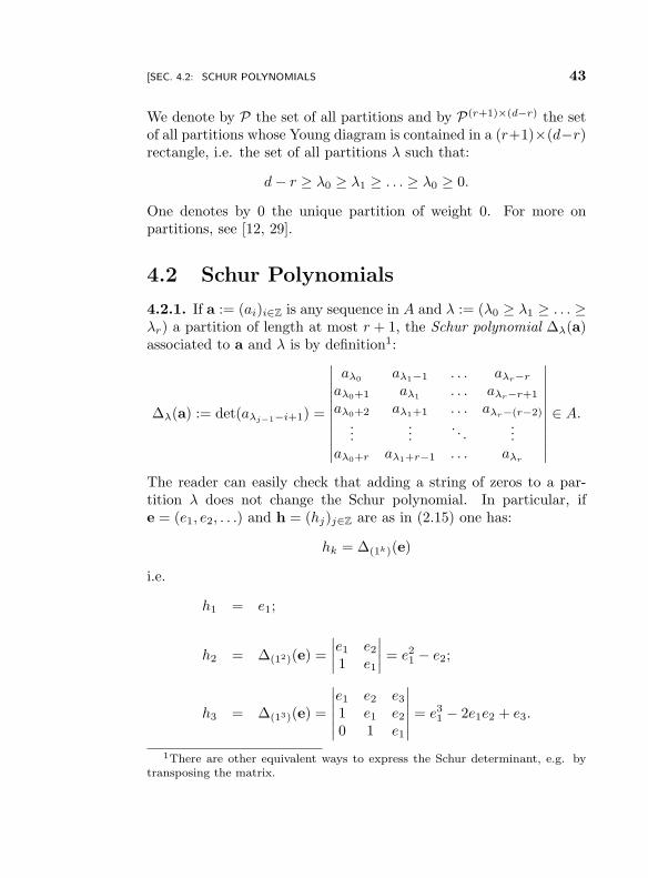
4.2.1. If a := (ai)i∈Z is any sequence in A and λ := (λ0 ≥ λ1 ≥ . . . ≥λr) a partition of length at most r + 1, the Schur polynomial ∆λ(a)associated to a and λ is by definition1:
∆λ(a) := det(aλj−1−i+1) =
∣∣∣∣∣∣∣∣∣∣∣
aλ0aλ1−1 . . . aλr−r
aλ0+1 aλ1. . . aλr−r+1
aλ0+2 aλ1+1 . . . aλr−(r−2)
......
. . ....
aλ0+r aλ1+r−1 . . . aλr
∣∣∣∣∣∣∣∣∣∣∣
∈ A.
The reader can easily check that adding a string of zeros to a par-tition λ does not change the Schur polynomial. In particular, ife = (e1, e2, . . .) and h = (hj)j∈Z are as in (2.15) one has:
hk = ∆(1k)(e)
i.e.
h1 = e1;
h2 = ∆(12)(e) =
∣∣∣∣e1 e21 e1
∣∣∣∣ = e21 − e2;
h3 = ∆(13)(e) =
∣∣∣∣∣∣
e1 e2 e31 e1 e20 1 e1
∣∣∣∣∣∣= e31 − 2e1e2 + e3.
1There are other equivalent ways to express the Schur determinant, e.g. bytransposing the matrix.
“EscoAlgtot˙New”2012/10/10page 44
i
i
i
i
i
i
i
i
44 [CAP. 4: GENERALIZED WRONSKIANS
In order to keep a simple and neat notation, for each partition λ weshall write:
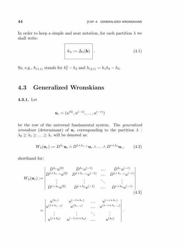
hλ := ∆λ(h) . (4.1)
So, e.g., h(1,1) stands for h21 − h2 and h(2,1) = h1h2 − h3.
4.3 Generalized Wronskians
4.3.1. Let
ur = (u(0), u(−1), . . . , u(−r))
be the row of the universal fundamental system. The generalizedwronskian (determinant) of ur corresponding to the partition λ :λ0 ≥ λ1 ≥ . . . ≥ λr will be denoted as:
Wλ(ur) := Dλrur ∧D1+λr−1ur ∧ . . . ∧D
r+λ0ur, (4.2)
shorthand for:
Wλ(ur) :=
∣∣∣∣∣∣∣∣∣
Dλru(0) Dλru(−1) . . . Dλru(−r)
D1+λr−1u(0) D1+λr−1u(−1) . . . D1+λr−1u(−r)
......
. . ....
Dr+λ0u(0) Dr+λ0u(−1) . . . Dr+λ0u(−r)
∣∣∣∣∣∣∣∣∣(4.3)
=
∣∣∣∣∣∣∣∣∣
u(λr) u(−1+λr) . . . u(−r+λr)
u(1+λr−1) u(λr−1) . . . u(1−r+λr−1)
......
. . ....
u(r+λ0) u(−1+r+λ0) . . . u(λ0)
∣∣∣∣∣∣∣∣∣
.
“EscoAlgtot˙New”2012/10/10page 45
i
i
i
i
i
i
i
i
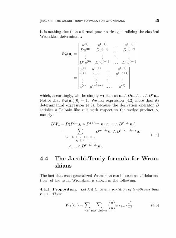
[SEC. 4.4: THE JACOBI-TRUDY FORMULA FOR WRONSKIANS 45
It is nothing else than a formal power series generalizing the classicalWronskian determinant:
W0(u) =
∣∣∣∣∣∣∣∣∣
u(0) u(−1) . . . u(−r)
Du(0) Du(−1) . . . Du(−r)
......
. . ....
Dru(0) Dru(−1) . . . Dru(−r)
∣∣∣∣∣∣∣∣∣
=
∣∣∣∣∣∣∣∣∣
u(0) u(−1) . . . u(−r)
u(1) u(0) . . . u(−r+1)
......
. . ....
u(r) u(−1+r) . . . u(0)
∣∣∣∣∣∣∣∣∣
which, accordingly, will be simply written as ur ∧Dur ∧ . . . ∧Drur.
Notice that W0(ur)(0) = 1. We like expression (4.2) more than itsdeterminantal expression (4.3), because the derivation operator Dsatisfies a Leibniz–like rule with respect to the wedge product ∧,namely:
DWλ = D(Dλrur ∧D1+λr−1ur ∧ . . . ∧D
r+λ0ur)
=∑
i0 + i1 + . . . + ir = 1ij ≥ 0
Di0+λrur ∧D1+i1+λr−1ur
∧ . . . ∧Dr+ir+λ0ur.
(4.4)
4.4 The Jacobi-Trudy formula for Wron-
skians
The fact that each generalized Wronskian can be seen as a “deforma-tion” of the usual Wronskian is shown in the following:
4.4.1. Proposition. Let λ ∈ ℓr be any partition of length less thanr + 1. Then:
Wλ(ur) =∑
n≥0
∑
µ∈ℓr,|µ|=n
(n
µ
)hλ+µ ·
tn
n!, (4.5)

“EscoAlgtot˙New”2012/10/10page 46
i
i
i
i
i
i
i
i
46 [CAP. 4: GENERALIZED WRONSKIANS
where if |µ| = n (n
µ
)=
n!
µ0!µ1! · . . . · µr!
is the coefficient of xµ := xµ0
0 xµ1
1 ·. . .·xµrr in the expansion of (x0+x1+
. . .+ xr)n. In particular, the constant term Wλ(ur)(0) of Wλ(ur) ishλ (see (4.1)) which, for λ = 0 (the null partition), yields W0(u)(0) =h0 = 1.
Proof. The transpose uTr of the row ur can be written as:
uTr =
∑
n≥0
hn
hn−1
...hn−r
·tn
n!.
By renaming n as µr−i, for each 0 ≤ i ≤ r, one easily finds:
Di+λr−iuTr =
∑
µr−i≥0
hλr−i+µr−i+i
hλr−i+µr−i+i−1
...hλr−i+µr−i+i−r
tµr−i
µr−i!.
Invoking the fact that the determinant of a matrix coincides with thedeterminant of the transpose, one can write:
Wλ(ur) = DλruTr ∧D1+λr−1uT
r ∧ . . . ∧Dr+λ0uTr =
=∑
µ∈ℓr
hλr+µr
hλr+µr−1
. . .hλr+µr−r
tµr
µr!∧
hλr−1+µr−1+1
hλr−1+µr−1
. . .hλr−1+µr−1−(r−1)
tµr−1
µr−1!∧ . . . ∧
hλ0+µ0+r
hλ0+µ0−1
. . .hλ0+µ0
tµ0
µ0!=
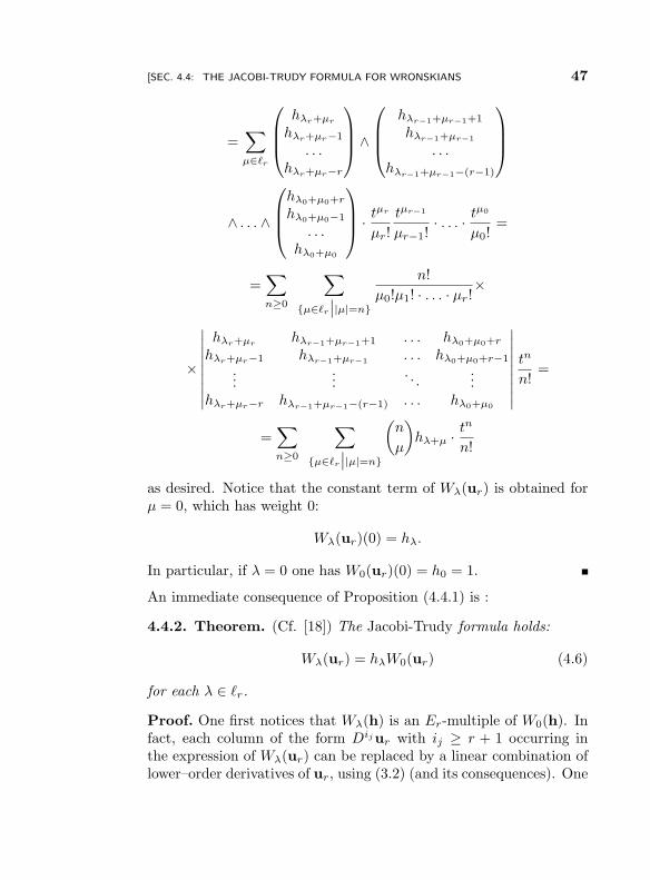
“EscoAlgtot˙New”2012/10/10page 47
i
i
i
i
i
i
i
i
[SEC. 4.4: THE JACOBI-TRUDY FORMULA FOR WRONSKIANS 47
=∑
µ∈ℓr
hλr+µr
hλr+µr−1
. . .hλr+µr−r
∧
hλr−1+µr−1+1
hλr−1+µr−1
. . .hλr−1+µr−1−(r−1)
∧ . . . ∧
hλ0+µ0+r
hλ0+µ0−1
. . .hλ0+µ0
·tµr
µr!
tµr−1
µr−1!· . . . ·
tµ0
µ0!=
=∑
n≥0
∑
µ∈ℓr
∣∣|µ|=n
n!
µ0!µ1! · . . . · µr!×
×
∣∣∣∣∣∣∣∣∣
hλr+µrhλr−1+µr−1+1 . . . hλ0+µ0+r
hλr+µr−1 hλr−1+µr−1. . . hλ0+µ0+r−1
......
. . ....
hλr+µr−r hλr−1+µr−1−(r−1) . . . hλ0+µ0
∣∣∣∣∣∣∣∣∣
tn
n!=
=∑
n≥0
∑
µ∈ℓr
∣∣|µ|=n
(n
µ
)hλ+µ ·
tn
n!
as desired. Notice that the constant term of Wλ(ur) is obtained forµ = 0, which has weight 0:
Wλ(ur)(0) = hλ.
In particular, if λ = 0 one has W0(ur)(0) = h0 = 1.
An immediate consequence of Proposition (4.4.1) is :
4.4.2. Theorem. (Cf. [18]) The Jacobi-Trudy formula holds:
Wλ(ur) = hλW0(ur) (4.6)
for each λ ∈ ℓr.
Proof. One first notices that Wλ(h) is an Er-multiple of W0(h). Infact, each column of the form Dijur with ij ≥ r + 1 occurring inthe expression of Wλ(ur) can be replaced by a linear combination oflower–order derivatives of ur, using (3.2) (and its consequences). One
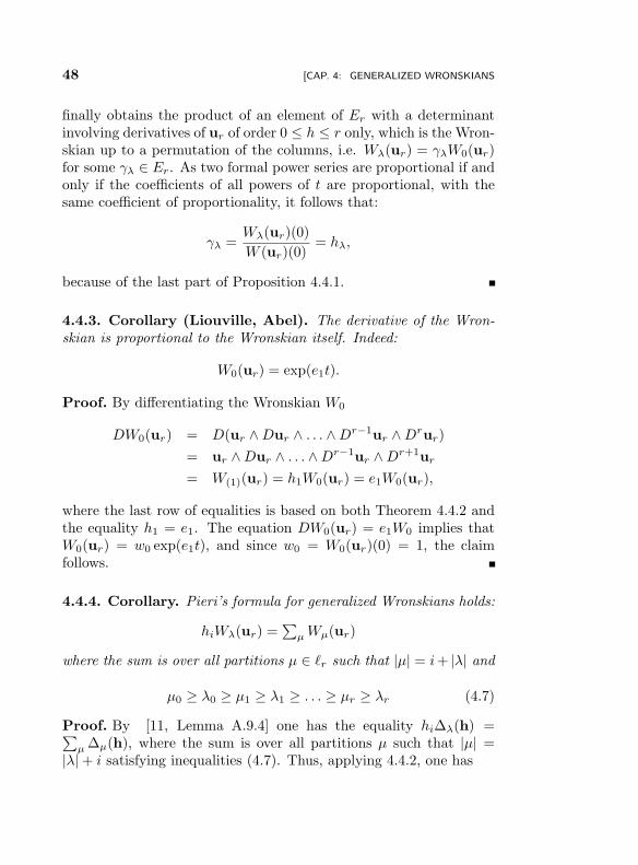
“EscoAlgtot˙New”2012/10/10page 48
i
i
i
i
i
i
i
i
48 [CAP. 4: GENERALIZED WRONSKIANS
finally obtains the product of an element of Er with a determinantinvolving derivatives of ur of order 0 ≤ h ≤ r only, which is the Wron-skian up to a permutation of the columns, i.e. Wλ(ur) = γλW0(ur)for some γλ ∈ Er. As two formal power series are proportional if andonly if the coefficients of all powers of t are proportional, with thesame coefficient of proportionality, it follows that:
γλ =Wλ(ur)(0)
W (ur)(0)= hλ,
because of the last part of Proposition 4.4.1.
4.4.3. Corollary (Liouville, Abel). The derivative of the Wron-skian is proportional to the Wronskian itself. Indeed:
W0(ur) = exp(e1t).
Proof. By differentiating the Wronskian W0
DW0(ur) = D(ur ∧Dur ∧ . . . ∧Dr−1ur ∧D
rur)
= ur ∧Dur ∧ . . . ∧Dr−1ur ∧D
r+1ur
= W(1)(ur) = h1W0(ur) = e1W0(ur),
where the last row of equalities is based on both Theorem 4.4.2 andthe equality h1 = e1. The equation DW0(ur) = e1W0 implies thatW0(ur) = w0 exp(e1t), and since w0 = W0(ur)(0) = 1, the claimfollows.
4.4.4. Corollary. Pieri’s formula for generalized Wronskians holds:
hiWλ(ur) =∑
µWµ(ur)
where the sum is over all partitions µ ∈ ℓr such that |µ| = i+ |λ| and
µ0 ≥ λ0 ≥ µ1 ≥ λ1 ≥ . . . ≥ µr ≥ λr (4.7)
Proof. By [11, Lemma A.9.4] one has the equality hi∆λ(h) =∑µ ∆µ(h), where the sum is over all partitions µ such that |µ| =
|λ| + i satisfying inequalities (4.7). Thus, applying 4.4.2, one has
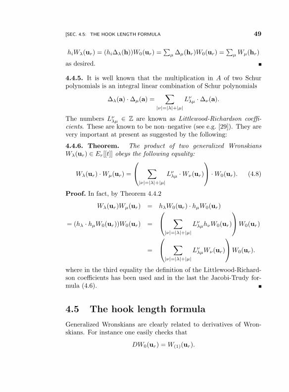
“EscoAlgtot˙New”2012/10/10page 49
i
i
i
i
i
i
i
i
[SEC. 4.5: THE HOOK LENGTH FORMULA 49
hiWλ(ur) = (hi∆λ(h))W0(ur) =∑
µ ∆µ(hr)W0(ur) =∑
µWµ(hr)
as desired.
4.4.5. It is well known that the multiplication in A of two Schurpolynomials is an integral linear combination of Schur polynomials
∆λ(a) · ∆µ(a) =∑
|ν|=|λ|+|µ|
Lνλµ · ∆ν(a).
The numbers Lνλµ ∈ Z are known as Littlewood-Richardson coeffi-
cients. These are known to be non–negative (see e.g. [29]). They arevery important at present as suggested by the following:
4.4.6. Theorem. The product of two generalized WronskiansWλ(ur) ∈ Er[[t]] obeys the following equality:
Wλ(ur) ·Wµ(ur) =
∑
|ν|=|λ|+|µ|
Lνλµ ·Wν(ur)
·W0(ur). (4.8)
Proof. In fact, by Theorem 4.4.2
Wλ(ur)Wµ(ur) = hλW0(ur) · hµW0(ur)
= (hλ · hµW0(ur))W0(ur) =
∑
|ν|=|λ|+|µ|
LνλµhνW0(ur)
W0(ur)
=
∑
|ν|=|λ|+|µ|
LνλµWν(ur)
W0(ur).
where in the third equality the definition of the Littlewood-Richard-son coefficients has been used and in the last the Jacobi-Trudy for-mula (4.6).
4.5 The hook length formula
Generalized Wronskians are clearly related to derivatives of Wron-skians. For instance one easily checks that
DW0(ur) = W(1)(ur).
“EscoAlgtot˙New”2012/10/10page 50
i
i
i
i
i
i
i
i
50 [CAP. 4: GENERALIZED WRONSKIANS
Differentiating a determinant is the same as applying Leibniz’s rulewith respect to the wedge product ∧. Using the fact that a determi-nant vanishes whenever two rows are equal, one gets:
DW0(ur) = D(ur ∧Dur ∧ . . . ∧Drur)
= ur ∧Dur ∧ . . . ∧Dr−1ur ∧D
r+1ur
= W(1)(ur).
The reader can easily convince himself that, in general, the j-thderivative of a wronskian is a linear combination of generalized Wron-skians:
DjW0(ur) =∑
|λ|=j
gλWλ(ur). (4.9)
This is a consequence of (4.4) and of an easy induction. It is wellknown that the Jacobi-Trudy formula, or its Pieri’s consequence, im-plies that the coefficient of Wλ(ur) in the expansion of hn
1W0(ur) canbe computed by means of the hook length formula (Cf. Section 4.5.1).In terms of generalized Wronskians, this property reads:
4.5.1. Theorem. (see [18]) The coefficient gλ in (4.9) can be com-puted by the hook length formula:
gλ =|λ|!
k1 · . . . · kj
=j!
k1 · . . . · kj
(4.10)
where ki is the hook length of each box of the Young diagram of thepartition λ .
Proof. In fact by the Liouville formula DjWλ(ur) = hjW0(ur), andthen one may apply the hook length formula holding for the multi-plication of hj
1 with a Schur polynomial hλ, as in [12].
A consequence of Theorem 4.5.1 is the following remarkable fact,already observed in [14] (see also Chapter 6):
4.5.2. Corollary. Let (d − r)r+1 be the partition with r + 1 partsequal to d−r. Then the coefficient g(d−r)r+1 multiplying W(d−r)r+1(ur)
in the expansion of D(r+1)(d−r)W0(ur) is precisely the Plucker degree
“EscoAlgtot˙New”2012/10/10page 51
i
i
i
i
i
i
i
i
[SEC. 4.5: THE HOOK LENGTH FORMULA 51
of the Grassmannian G(r,Pd), parameterizing r dimensional linearsubvarieties in the complex projective space, i.e.:
g(d−r)r+1 =1!2! · . . . · r! · (r + 1)(d− r)!
(d− r)!(d− r + 1)! · . . . · d!.
4.5.3. Example. Let u1 = (u(0), u(−1)). Then:
D4W0(u1) := D4(u1 ∧Du1) = D3 D(u1 ∧Du1)
= D3(u1 ∧D2u1) = D2(Du1 ∧D
2u1 + u1 ∧D3u1)
= D(2 ·Du1 ∧D3u1 + u1 ∧D
4u1)
= 2 ·D2u1 ∧D3u1 + 3 ·Du1 ∧D
4u1 + u1 ∧D5u1
= 2 ·D0+2u1 ∧D1+2u1 + 3 ·D0+1u1 ∧D
1+3f
+ u1 ∧D1+4u1
= 2 ·W(2,2)(u1) + 3 ·W(3,1)(u1) +W(4)(u1).
The coefficient 2 multiplying W(2,2)(u1) is precisely the Plucker de-gree of the Grassmannian G(1,P3) in its Plucker embedding, i.e thenumber of lines meeting 4 others in general position – see [13, 14] fordetails. All other coefficients have an enumerative interpretation ineither the classical or the quantum cohomology of the Grassmannian(see e.g. [14]).
“EscoAlgtot˙New”2012/10/10page 52
i
i
i
i
i
i
i
i
Chapter 5
Exponential of matrices
5.1 A brief historical account.
5.1.1. Any system of linear ODEs with constant coefficients:
x1 = a11x1 + a12x2 + . . .+ a1nxn
x2 = a21x1 + a22x2 + . . .+ a2nxn
......
xn = an1x1 + an2x2 + . . .+ annxn
in the unknown functions xi : D ⊆ C → C can be written in matrixform as:
x = M · x,
where x is the column of the unknown functions xi and M is the (con-stant) matrix of the coefficients (aij). It is known that the solutionof the system is of the form
x = exp(tM) · c (5.1)
where c ∈ Cn is a column of constants depending on the initial con-dition x(0). If M is a square matrix, its exponential exp(M) is aninvertible square matrix defined by extending formally the definition
52
“EscoAlgtot˙New”2012/10/10page 53
i
i
i
i
i
i
i
i
[SEC. 5.1: A BRIEF HISTORICAL ACCOUNT. 53
of the exponential of a complex number:
exp(M) := 1 +M +M2
2!+ . . . =
∑
n≥0
Mn
n!. (5.2)
One is naturally led to wonder if the exponential of a matrix definedin this way is a matrix itself, i.e. if the series (5.2) is convergent. Thiscan be easily done. Indeed
exp(tM) =∑
n≥0
Mntn
n!
converges for each t ∈ C and then it defines a family of inverti-ble square matrices. The second problem is to computing it. Tothis purpose one uses the fact that if P is any invertible matrix,then exp(P−1MP ) = P−1 exp(M)P . Over the complex numbers oneknows that each matrix is conjugated to an essentially unique matrixin Jordan normal form JM . Then
exp(A) = exp(P−1JAP ) = P−1 exp(JA)P
and the problem is reduced to compute the exponential of a matrixwhich is already in Jordan normal form. This is easy, because anysuch matrix can be written as a block matrix, whose blocks are sumsD + N of a diagonal and a nilpotent matrix commuting with oneanother. The exponential of any such block is exp(N) exp(D). Usingsuch a procedure, all the technical issues due to the computation ofthe exponential of a matrix are reduced to the problem of computinga canonical Jordan form of it. Such a computation can be howeveravoided, as noted by E. J. Putzer, in a paper appeared on Ameri-can Mathematical Monthly [33] in 1966. Before explaining Putzer’smethod let us make a comment. To show that exp(Mt) · c is a solu-tion of (5.1) one has just to compute its first derivative with respectto t in a purely formal way:
d
dtexp(tM) =
d
dt
∑
n≥0
Mntn
n!=∑
n≥1
Mntn
n!= M+M2t+M3 t
2
2+ . . . =
= M
(1 +Mt+
M2t2
2!+ . . .
)= M exp(tM).
“EscoAlgtot˙New”2012/10/10page 54
i
i
i
i
i
i
i
i
54 [CAP. 5: EXPONENTIAL OF MATRICES
Thus exp(tM)c satisfies (5.1) for purely formal reasons, a remarksuggesting that much important information can possibly be obtainedby considering the exponential of a matrix in a purely formal way.
5.1.2. Putzer’s idea. As well known, each square matrix A ∈Cn×n satisfies at least one polynomial identity (indeed many poly-nomial identities), e.g. it is a zero of its characteristic polynomialby the Cayley–Hamilton theorem. In other words, the exponentialof M , if it exists, can be written as a complex linear combination of1,M,M2, . . . ,Mn−1,
exp(M) = α01 + α1M + α2M2 + . . .+ αn−1M
n−1,
and the task consists now in computing such coefficients. Putzer(1966, [33]) solves the problem by considering the exponential exp(Mt)which, because of the Cayley–Hamilton theorem, can be written inthe form:
exp(tM) = α0(t)1 + α1(t)M + . . .+ αn−1(t)Mn−1, (5.3)
where α0, α1, . . . , αn−1 should be suitable holomorphic functions.This is indeed the case and in [33] the author is able to describeprecisely all coefficients αi occurring into the expression (5.3). LetPM (t) be the characteristic polynomial of the matrix M . Then thecoefficient αn−1(t) is the unique solution of the Cauchy ProblemPM (D)y = 0 such that y(i) = 0 for 0 ≤ i ≤ n − 2 and yn−1(0) =1 (which is a generator of the impulsive response kernel, see Re-mark 3.2.2). Once the coefficient αn−1 is known, Putzer gives aprecise description of how to determine the remaining coefficients,based on the sole knowledge of αn−1. To apply his method, however,the author needs to find the roots of the characteristic polynomial,in order to express αn−1 as a linear combination of a fundamentalsystem of solutions.
5.1.3. Although Putzer’s description of the computation ofα1, . . . , αn−2 occurring in (5.3) is very precise, the Author proposesno interpretation of them. The latter is offered in a couple of shortpapers by I. H. Leonard [28] (1996) and E. Liz [27] (1998), publishedin the SIAM journal. They show that, for each 0 ≤ i ≤ n − 1, thefunction αi is the unique solution of the Cauchy problem PA(D)y = 0
“EscoAlgtot˙New”2012/10/10page 55
i
i
i
i
i
i
i
i
[SEC. 5.2: THE MATRIX EXPONENTIAL 55
satisfying the initial condition y(j)i (0) = δij . This result, although
very elementary, is beautiful and elegant. To compute the exponen-tial of a matrix, however, even the aforementioned authors have tocope with the technical issue of finding the roots of the characteristicpolynomial. The purpose of next section is to show that workingformally the matter gets easier, basing on the results of the previousChapters.
5.2 The matrix exponential
5.2.1. Let M := (aij) ∈ An×n be a square matrix with entries in theEr-algebra A and let t be an indeterminate over A. Then M · t is asquare matrix with entries in A[t] ⊆ A[[t]]. Define:
exp(Mt) :=∑
n≥0
Mntn
n!
tviewed as a matrix of formal power series, under the identificationA[[t]]n×n ∼= An×n[[t]]. Notice that P ∈ A[t] |P (M) = 0 is non–
empty. In fact 1,M,M2, . . . ,Mn2
are n2 + 1 matrices living in thefree module An×n of rank n2, and thus they are linearly dependent.The Cayley-Hamilton theorem holds for A-valued matrices as well:each matrix M ∈ An×n is a zero of its characteristic polynomial, i.e.
PM (t) = det(M − t1).
In other words Mn+j is an A-linear combination of 1,M, . . . ,Mn−1
and so exp(Mt) must be a linear combination of (1,M, . . . ,Mn−1) aswell, with coefficients in A[[t]]. To determine the coefficients we shallfirst analyze the case when M is the companion matrix associated tothe universal ODE (3.3). See below.
5.3 The exponential of a companion ma-
trix
5.3.1. Let e1, . . . , en be the canonical basis of An thought of as theA-module of the columns of n elements of A. The entries of the
“EscoAlgtot˙New”2012/10/10page 56
i
i
i
i
i
i
i
i
56 [CAP. 5: EXPONENTIAL OF MATRICES
column ej are 0 except the i–th which is equal to 1. One says thata := (ai) ∈ An is the initial condition of a solution of the linear ODE:P (D)y = 0 if and only if y(i)(0) = ai.
5.3.2. The universal ODE: Ur+1(D)y = 0 can be equivalently writtenas a system of differential equations:
y(1) = y1,
y(1)1 = y2,...
......
y(1)r = e1yr − e2yr−1 + . . .+ (−1)rer+1y,
or, more compactly:Y (1) = Cr · Y
where
Y :=
y
y1...yr
, and
Cr :=
0 1 0 . . . 00 0 1 . . . 0...
......
. . ....
(−1)rer+1 (−1)r−1er (−1)r−2er−1 . . . e1
. (5.4)
The matrix Cr is the companion matrix associated to the polynomialUr+1(t) ∈ Er[t] and Y (1) is the column of the derivatives of the entriesof Y , with respect to the indeterminate t. For purely formal (and notsubstantial) reasons, we shall regard Cr as an endomorphism of theEr-module Er ⊕Er
r of columns of (r + 1) elements of Er, with basise0, e1, . . . , er:
e0 =
10...0
= 1 ⊕ 0Er
r, e1 =
01...0
, er =
00...1
.
So, in particular, the columns of Cr are numbered from 0 to r.
“EscoAlgtot˙New”2012/10/10page 57
i
i
i
i
i
i
i
i
[SEC. 5.3: THE EXPONENTIAL OF A COMPANION MATRIX 57
5.3.3. Proposition. Let αi, 0 ≤ i ≤ r, be the unique element ofkerUr+1(D) such that (Djαi)(0) = δij. The matrix exp(Crt) is theWronskian matrix associated to the fundamental system of solutions(α0, α1, . . . , αr).
Proof. For each 0 ≤ j ≤ r
Y = exp(Crt)ej
is a solution of the system such that Y (0) = ej , i.e. it correspondsto the unique solution αj(t) of the linear ODE: Ur+1(D)y = 0, suchthat y(j)(0) = 1 and yi(0) = 0, for all i 6= j. On the other handexp(Crt)ej is the (j + 1)-th column of exp(Crt), i.e.:
exp(Crt)ej =
αj
α′j
...
α(r)j
.
Then
exp(Crt) =
α0 α1 . . . αr
α(1)0 α
(1)1 . . . α
(1)r
......
. . ....
α(r)0 α
(r)1 . . . α
(r)r
as claimed.
5.3.4. We are now in the position to give a precise expression of theexponential of Cr. By the universal Cauchy formula (3.11) one has:
αj =
r∑
i=0
Ui(ej)u(−i)
i.e.:
α0 = u(0) − e1u(−1) + e2u
(−2) + . . .+ (−1)reru(−r).
α1 = u(−1) − e1u(−2) + . . .+ (−1)reru
(−r)
... =...
αr = u(−r).

“EscoAlgtot˙New”2012/10/10page 58
i
i
i
i
i
i
i
i
58 [CAP. 5: EXPONENTIAL OF MATRICES
5.3.5. Example. To compute the exponential of
C2 :=
0 1 00 0 1e3 −e2 e1
we consider the solutions α1, α2, α3 of the linear ODE: U2(D)y = 0, havinge0, e1, e2 as initial conditions. Then:
α0 = u(0) − e1u
(−1) + e2u(−2)
, α1 = u(−1) − e1u
(−2), α2 = u
(−2),
from which
α(1)0 = u
(1) − e1u(0) + e2u
(−1), α
(1)1 = u
(0) − e1u(−1)
, α2 = u(−1)
.
One uses now the fact that
u(1) = e1u
(0) − e2u(−1) + e3u
(−2),
which substituted into the expression of α(1)0 gives α
(1)0 = e3u
(−2). Hence:
α(2)0 = e3u
(−1), α
(2)1 = −e2u(−1) + e3u
(−2), α2 = u
(0).
In conclusion, the exponential of C2 is:
exp(C2t) =
u(0) − e1u
(−1) + e2u(−2) u(−1) − e1u
(−2) u(−2)
e3u(−2) u(0) − e1u
(−1) u(−1)
e3u(−1) −e2u(−1) + e3u
(−2) u(0)
.
5.3.6. Lemma. For 1 ≤ j ≤ r, all entries of the first row of Cjr are
0 but the j–th, which is equal to 1.
Proof. For 0 ≤ i ≤ r, let ǫi = eTi be the row which has all entries 0
but the i–th which is equal to 1. Then the first row of Cjr is given by
the matrix product ǫi · Cjr . Now
Cr =
ǫ1
ǫ2
...ǫr
(−1)rer+1ǫ0 + (−1)r−1erǫ
1 + . . .+ e1ǫr
.
“EscoAlgtot˙New”2012/10/10page 59
i
i
i
i
i
i
i
i
[SEC. 5.3: THE EXPONENTIAL OF A COMPANION MATRIX 59
We claim that for j − 1 ≤ r − 1 one has:
Cjr =
ǫj
ǫj+1
...ǫr
...
.
The property is true for j = 1. Suppose it holds for 1 ≤ j−1 ≤ r−1.Then
Cjr = Cr · C
j−1r =
ǫ1 · Cj−1r
ǫ2 · Cj−1r
...ǫr−j−1 · Cj−1
r
...
=
ǫj
ǫj+1
...ǫr
...
by inductive hypothesis. In particular the first row of Cjr is ǫ0 ·Cj
r = ǫj
as claimed.
5.3.7. Proposition. The exponential of the companion matrix Cr
is:exp(Crt) = α11 + α2Cr + . . .+ αr+1C
rr . (5.5)
Proof. The characteristic polynomial of Cr is precisely Ur+1(t).Hence Cn
r is a linear combination of 1, Cr, . . . , Crr for each n ≥ r+ 1,
and thus the exponential of Crt can be expressed as a linear combi-nation
exp(Crt) = λ01 + λ1Cr + . . .+ λrCrr , (5.6)
where λ0, λ1, . . . , λr ∈ Er[[t]]. Then (5.6) implies
ǫ0 · exp(Crt) = λ0ǫ01 + λ1ǫ
0Cr + . . .+ λrǫ0Cr
r .
By Lemma (5.3.6) the first row of Cjr is precisely ǫj and so by Propo-
sition 5.3.3 one has the equality:
(α0, α1, . . . , αr) = λ0ǫ0 + λ1ǫ
1 + . . .+ λrǫr = (λ0, λ1, . . . , λr),
whence λj = αj , for all 0 ≤ j ≤ r.
“EscoAlgtot˙New”2012/10/10page 60
i
i
i
i
i
i
i
i
60 [CAP. 5: EXPONENTIAL OF MATRICES
5.3.8. If A is any Q-algebra and P ∈ A[t] is a monic polynomial ofdegree r+1, we shall denote by CP the companion matrix associatedto P , i.e.
CP :=
0 1 0 . . . 00 0 1 . . . 0...
......
. . ....
(−1)rer+1(P ) (−1)r−1er(P ) (−1)r−2er−1(P ) . . . e1(P )
(5.7)
where ei(P ) ∈ A. Let βi := φP (αi) be the image of the universal basis(α0, α1, . . . , αr) of kerUr+1(D) through the unique homomorphismφ : Er → A mapping ei 7→ ei(P ). Then
exp(CP t) = β01 + β1CP + . . .+ βrCrP .
5.3.9. Given a m×m matrix, let P ∈ A[t] be any monic polynomialof degree r + 1 vanishing at M , i.e. P (M) = 0. If P were thecharacteristic polynomial of M , then r+1 = m, if P were the minimalpolynomial of M then r+1 ≤ m. The degree of P may also be biggerthan m and, of course, any such polynomial would be a multiple ofthe minimal polynomial. Suppose now that β0, β1, . . . , βr ∈ A[[t]] arethe unique solutions of the Cauchy problem P (D)y = 0 with initialconditions ei, 1 ≤ i ≤ n.
5.3.10. Theorem.
exp(M · t) = β01 + β1M + . . .+ βrMr.
Proof. By definition of exponential of a matrix, one has:
exp(Mt) =∑
n≥0
Mn tn
n!
=
r∑
n=0
Mn tn
n!+Mr+1 tr+1
(r + 1)!+Mr+2 tr+2
(r + 2)!+ . . .
Now Mr+1 = e1(P )Mr + . . . + (−1)rer+1(P )1 and, by induction,each Mn, for n ≥ r + 1, can be expressed as a linear combination of1,M, . . . ,Mr. Therefore the exponential of M · t is:
exp(M · t) = λ01 + λ1M + . . .+ λrMr, λi ∈ A[t]].
“EscoAlgtot˙New”2012/10/10page 61
i
i
i
i
i
i
i
i
[SEC. 5.4: SOME PROPERTIES OF THE EXPONENTIAL 61
The coefficients λi are determined in a purely formal way using therelation P (M) = 0 and do not depend on the choice of the matrix.So, in particular, they are the same that one would find if M werethe companion matrix CP associated to P . In this case, by 5.3.8,λ0, λ1, . . . , λr are precisely the unique solutions (β0, β1, . . . , βr) of theCauchy problem P (D)y = 0 with initial conditions (Diβj)(0) = δij .
5.4 Some properties of the exponential
The A-module An×n of A-valued n × n matrices is a Lie A-algebra,with respect to the commutator:
[M,N ] = MN −NM.
5.4.1. Proposition. Let M,N ∈ An×n. Then
exp(M +N) = exp(M) exp(N) (5.8)
if and only if [M,N ] = 0.
Proof. It is enough to compare the summands of degree 2 on bothsides of (5.8). The summand of degree 2 in the expansion of exp(M+N) is
(M +N)(M +N)
2=M2 +MN +NM +N2
2,
while that in the expansion of exp(M) exp(N) is
M2 + 2MN +N2
2.
Equality (5.8) implies
M2 +MN +NM +N2 = M2 + 2MN +N2,
i.e. MN = NM . Conversely if [M,N ] = 0,
(M +N)n
n!=
∑nh=0
(nh
)MhNn−h
n!
which coincides precisely with the summand of degree n in the ex-pansion of exp(A) exp(B).
“EscoAlgtot˙New”2012/10/10page 62
i
i
i
i
i
i
i
i
62 [CAP. 5: EXPONENTIAL OF MATRICES
5.4.2. Let M ∈ Am×m and N ∈ An×n. Denote by M ⊕N the blockdiagonal(m+ n) × (m+ n) matrix
M ⊕N :=
M 0m×n
0n×m N
.
The notation is motivated by the fact that M ⊕N , when seen as anendomorphism of Am+n, decomposes the latter into the direct sumof M and N -invariant subspaces:
Am+n = (Am ⊕ 0n) ⊕ (0m ⊕An).
By induction one easily proves that:
det(M1 ⊕ . . .⊕Mh) = det(M1) · . . . · det(Mh),
andtr(M1 ⊕ . . .⊕Mh) = tr(M1) + . . .+ tr(Mh).
Finally, it is clear that
exp((M1 ⊕ . . .⊕Mh)t) = exp(M1t) ⊕ . . .⊕ exp(Mht).
5.4.3. Lemma. Let CP be the companion matrix associated to amonic polynomial P ∈ A[t] of degree r + 1 (r ≥ 0). Then
det(exp(CP t)) = exp(tr(CP )t).
Proof. By the expression (5.7) it is clear that tr(CP ) = e1(P ). Nowexp(CP t) is the Wronskian W = W (β0, β1, . . . , βr) of the fundamen-tal system of solutions βi such that Djβi(0) = δij . By Proposi-tion 4.4.3 one knows that
W = exp(CP t) = exp(e1(P )t) = exp(tr(CP t)),
and the claim is proven.
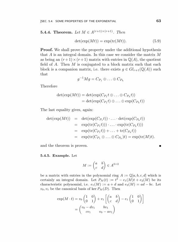
“EscoAlgtot˙New”2012/10/10page 63
i
i
i
i
i
i
i
i
[SEC. 5.4: SOME PROPERTIES OF THE EXPONENTIAL 63
5.4.4. Theorem. Let M ∈ A(r+1)×(r+1). Then
det(exp(Mt)) = exp(tr(Mt)). (5.9)
Proof. We shall prove the property under the additional hypothesisthat A is an integral domain. In this case we consider the matrix Mas being an (r+1)× (r+1) matrix with entries in Q(A), the quotientfield of A. Then M is conjugated to a block matrix such that eachblock is a companion matrix, i.e. there exists g ∈ Glr+1(Q(A)) suchthat
g−1Mg = CP1⊕ . . .⊕ CPh
Therefore
det(exp(Mt)) = det(exp(CP1t⊕ . . .⊕ CPh
t))
= det(exp(CP1t) ⊕ . . .⊕ exp(CPh
t))
The last equality gives, again:
det(exp(Mt)) = det(exp(CP1t)) · . . . · det(exp(CPh
t))
= exp(tr(CP1t))) · . . . · exp(tr(CPh
t)))
= exp(tr(CP1t)) + . . .+ tr(CPh
t))
= exp(tr(CP1⊕ . . .⊕ CPh
)t) = exp(tr(M)t).
and the theorem is proven.
5.4.5. Example. Let
M :=
(a b
c d
)∈ A
2×2
be a matrix with entries in the polynomial ring A := Q[a, b, c, d] which iscertainly an integral domain. Let PM (t) := t2 − e1(M)t + e2(M) be itscharacteristic polynomial, i.e. e1(M) := a + d and e2(M) = ad − bc. Letv0, v1 be the canonical basis of kerPM (D). Then
exp(M · t) = v0
(1 00 1
)+ v1
[(a b
c d
)− e1
(1 00 1
)]
=
(v0 − dv1 bv1cv1 v0 − av1
)
“EscoAlgtot˙New”2012/10/10page 64
i
i
i
i
i
i
i
i
64 [CAP. 5: EXPONENTIAL OF MATRICES
Equation (5.9) says that
v20 − e1(M)v0v1 + e2(M)v2
2 = exp(e1t) , (5.10)
which is the generalization of the celebrated equation
cos2 t+ sin2t = 1.
In fact if e1(M) = 0 and e2(M) = 1, the solutions v0, v1 occurring in (5.10)are precisely cos t and sin t while exp(e1(M)t) = exp(0 · t) = 1.
“EscoAlgtot˙New”2012/10/10page 65
i
i
i
i
i
i
i
i
Chapter 6
Derivations on an
Exterior Algebra
This chapter aims to provide a quick overview of the theory developedin [13, 14, 17] which will be applied to the situation we are mostlyinterested in, regarding modules of solutions of linear ODEs. Thosepapers mainly motivated the research carried out in [18].
6.1 Schubert Calculus on a Grassmann
Algebra
6.1.1. Given a graded integral Q-algebra A := ⊕i≥0Ai, finitelygenerated as an A0-algebra, consider the quotient
Mp :=A[t]
(p)
where p := td+1−e1(p)td+. . .+(−1)d+1ed+1(p) is a monic polynomialof degree d+ 1, such that ei(p) ∈ Ai. For each j ≥ 0 let
ǫj := tj + (p)
65
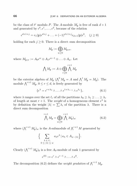
“EscoAlgtot˙New”2012/10/10page 66
i
i
i
i
i
i
i
i
66 [CAP. 6: DERIVATIONS ON AN EXTERIOR ALGEBRA
be the class of tj modulo P . The A-module Mp is free of rank d+ 1and generated by ǫ0, ǫ1, . . . , ǫd, because of the relation
ǫd+1+j = e1(p)ǫd+j + . . .+ (−1)d+1+jed+1(p)ǫ0, (j ≥ 0)
holding for each j ≥ 0. There is a direct–sum decomposition
Mp :=⊕
w≥0
Mp,w,
where Mp,w := A0ǫw ⊕A1ǫ
w−1 ⊕ . . .⊕Aw. Let
∧Mp := A⊕
⊕
r≥0
r+1∧Mp
be the exterior algebra of Mp (∧0
Mp = A and∧1
Mp = Mp). The
module∧r+1
Mp, 0 ≤ r ≤ d, is freely generated by
ǫλ = ǫr+λ0 ∧ . . . ∧ ǫ1+λr−1 ∧ ǫλr, (6.1)
where λ ranges over the set ℓr of all the partitions λ0 ≥ λ1 ≥ . . . ≥ λr
of length at most r + 1. The weight of a homogeneous element ǫλ isby definition the weight |λ| =
∑λi of the partition λ. There is a
direct sum decomposition
r+1∧Mp =
⊕
w≥0
(
r+1∧Mp)w (6.2)
where (∧r+1
Mp)w is the A-submodule of∧r+1
M generated by
∑
λ ∈ ℓr
0 ≤ |λ| ≤ w
aλǫλ | aλ ∈ Aw−|λ|
.
Clearly (∧r+1
Mp)0 is a free A0-module of rank 1 generated by
ǫ(0) := ǫr ∧ ǫr−1 ∧ . . . ∧ ǫ0.
The decomposition (6.2) defines the weight gradation of∧r+1
Mp.
“EscoAlgtot˙New”2012/10/10page 67
i
i
i
i
i
i
i
i
[SEC. 6.1: SCHUBERT CALCULUS ON A GRASSMANN ALGEBRA 67
6.1.2. Let us consider now the A-algebra∧Mp[[t]] of formal power
series with∧Mp-coefficients. The product is defined by
(∑
i≥0
piti) ∧ (
∑
j≥0
qjti) =
∑
n≥0
(∑
i+j=n
pi ∧ qj)tn.
Next, one considers EndA(∧Mp)[[t]], the A-algebra of formal power
series with coefficients in the (non commutative) A-algebra of endo-morphisms of
∧Mp. Each element
Dt := D0 +D1t+ . . . ∈ EndA(∧Mp)[[t]], (6.3)
can be regarded as anA-module homomorphismDt :∧Mp→
∧Mp[[t]]
via the obvious map p 7→ Dt(p) =∑
i≥0Dip · ti.
6.1.3. Definition. A formal power series (6.3) is a derivation onthe exterior algebra if
Dt(p ∧ q) = Dtp ∧Dtq, (p,q ∈∧M), (6.4)
i.e. if the map Dt :∧Mp →
∧Mp[[t]] is an A-algebra homomor-
phism.
Condition (6.4) implies that the homomorphism Dt is uniquelydefined once one knows how it operates on M – the degree 1 part ofthe exterior algebra.
6.1.4. Definition. The Schubert derivation on∧Mp is the unique
derivation such that that Djǫi = ǫi+j.
The reason for such a terminology, adopted in [14], is that Equa-tion (6.4), the fundamental equation of Schubert Calculus, presidesthe formalism of the intersection theory on Grassmann bundles – seebelow. Observe that each Di :
∧Mp →
∧Mp is a homomorphism of
degree 0, i.e. Di(∧1+r
M) ⊆∧r+1
Mp. By its very definition, it is
homogeneous of degree i on each∧r+1
Mp with respect to the weightgraduation:
Di(
r+1∧Mp)w ⊆ (
r+1∧Mp)w+i.
“EscoAlgtot˙New”2012/10/10page 68
i
i
i
i
i
i
i
i
68 [CAP. 6: DERIVATIONS ON AN EXTERIOR ALGEBRA
Moreover DiDj = DjDi, for each i, j ≥ 0. Let
A[T] := A[T1, T2, . . .]
be the polynomial ring in infinitely many indeterminates with A-coefficients. Each indeterminate Ti is given degree i. For a polyno-mial Q ∈ A[T], let Q(D) be its evaluation at D := (D0,D1, . . . , )through the map Ti 7→ Di. It turns out that A[D] := evD(A[T]) is acommutative subring of EndA(
∧Mp).
6.1.5. Proposition. The natural evaluation map
evǫ(0) : A[D] −→∧r+1
MP
Q(D) 7−→ Q(D)ǫ(0)(6.5)
is onto.
Proof. To show the surjectivity of the map (6.5) it is sufficient toshow that for each λ ∈ ℓr there exists Qλ ∈ A[T] such that ǫλ =Qλ(D) · ǫ(0). Then one argues by integration by parts as in [14]. Seethe example below.
6.1.6. Example. Consider ǫ(1,1) = ǫ2 ∧ ǫ1. Then
ǫ2 ∧ ǫ1 = ǫ
2 ∧D1ǫ0
= D1(ǫ2 ∧ ǫ0) − (D1ǫ
2) ∧ ǫ0
= D1(D1ǫ1 ∧ ǫ0) − ǫ
3 ∧ ǫ0
= D21ǫ
1 ∧ ǫ0 −D2(ǫ1 ∧ ǫ0) = (D2
1 −D2)ǫ0.
In other words:
ǫ(1,1) =
∣∣∣∣D1 1D2 D1
∣∣∣∣ ǫ1 ∧ ǫ0 = ∆(1,1)(D).
In general, one can show that Giambelli’s formula holds:
ǫλ = ∆λ(D)ǫ0, (6.6)
where ∆λ(D) is the Schur determinant associated to the sequenceD := (D0,D1, . . .) corresponding to the partition λ. Formula (6.6) isequivalent to Pieri’s formula:
Dhǫλ =
∑
µ∈ℓr,h,λ
ǫµ (h ≥ 0),
“EscoAlgtot˙New”2012/10/10page 69
i
i
i
i
i
i
i
i
[SEC. 6.1: SCHUBERT CALCULUS ON A GRASSMANN ALGEBRA 69
where
ℓr,h,λ =
partitions µ ∈ ℓr such that |µ| = |λ| + h andµ0 ≥ λ0 ≥ µ1 ≥ λ1 ≥ . . . ≥ µr ≥ λr ≥ 0
. (6.7)
6.1.7. Let
A∗(
r+1∧Mp) :=
A[D]
(ker evǫ0).
By construction,∧r+1
Mp is a free A∗(∧r+1
Mp)-module of rank 1generated by ǫ(0) = ǫr ∧ . . . ∧ ǫ1 ∧ ǫ0. The module multiplication isgiven by the A-bilinear map:
A∗(
r+1∧Mp) ⊗
r+1∧Mp −→
r+1∧Mp
given by (Q(D) + ker evǫ(0) , ǫλ) 7→ Q(D)ǫλ.
6.1.8. Remark. It turns out that A∗(∧r+1
MP ) is the universal splittingalgebra of the polynomial p as the product of two monic polynomials oneof degree r + 1. See e.g. [10, 24, 25].
6.1.9. Example. Let p,q ∈ ∧Mp. Then Newton’s Binomial formulafor D1 holds, i.e.:
Dm1 (p ∧ q) =
m∑
k=0
(m
k
)D
k1p ∧Dm−k
q. (6.8)
This is easily seen by induction. If m = 1 it is just Leibniz’s rule:
D1(p ∧ q) = D1p ∧ q + p ∧D1q.
For m = 2:
D21(p ∧ q) = D1[D1p ∧ q + p ∧D1q]
= D11p ∧ q +D1p ∧D1q +D1p ∧D1q + p ∧D2
1q
= D11p ∧ q + 2 ·D1p ∧D1q + p ∧D2
1q.
If (6.8) holds for h = m− 1 ≥ 1 it holds for m. In fact
Dm1 (p ∧ q) = D1(D
(m−11 (p ∧ q))
= D1
m−1∑
k=0
(m− 1
k
)D
k1p ∧Dm−1−k
1 q.
See [8] for generalizations and applications to the enumerative geometry ofrational space curves.
“EscoAlgtot˙New”2012/10/10page 70
i
i
i
i
i
i
i
i
70 [CAP. 6: DERIVATIONS ON AN EXTERIOR ALGEBRA
6.2 Connection with Schubert Calculus
Schubert calculus rules the intersection theory on Grassmann bun-dles. We give here a quick account to illustrate its relationships withthe derivations on a Grassmann algebra. Detailed references for thissection are [13, 14, 17, 24, 25]. The original motivation was to studyloci of Weierstrass points on families of possible singular Gorensteincurves (which exclude, therefore, the case studied in [34]). For anice survey about some combinatorics related with ramification lociof linear systems which inspired the present work see e.g. [7].
6.2.1. Each smooth complex projective variety X can be equippedwith an intersection theory, by attaching to X an Abelian groupA∗(X) and a Z-algebra A∗(X) which are isomorphic as Z-modules(Poincare duality). The group A∗(X) is generated by cycles modulorational equivalence and is a free module of rank 1 over A∗(X) gener-ated by the fundamental class [X]. The A∗(X)-module multiplicationof A∗(X) is said cap product:
A∗(X) ⊗Z A∗(X)∩
−→ A∗(X)
sending (α, c) 7→ α ∩ c ∈ A∗(X). See [11].
6.2.2. Example. The intersection theory of the projective space may bedescribed by saying that A∗(P
n) is a Z-module freely generated by the classof linear subvarieties of codimension i, for 0 ≤ i ≤ n:
A∗(Pn) = Z[Pn] ⊕ Z ·H ⊕ Z ·H2 ⊕ . . .⊕ Z ·Hn
.
The generator Hi is the class modulo rational equivalence of any linearsubvariety of codimenion i. The generator [Pn] is the fundamental class,whileHn is the class of a point. The class of each subvariety of codimensioni is of the form d ·Hi and the integer d is called the degree of the subvariety.The Chow ring of Pn is
A∗(Pn) =
Z[H]
(Hn+1)
and says what is the dimension and the degree of the intersection of ahyperplane and a projective subvariety of Pn in general position. Therelation Hn+1 = 0 expresses the fact that the intersection of (n + 1)-hyperplanes in general position is empty. The cap product H ∩ [S] is the
“EscoAlgtot˙New”2012/10/10page 71
i
i
i
i
i
i
i
i
[SEC. 6.2: CONNECTION WITH SCHUBERT CALCULUS 71
operation of cutting with a hyperplane. If S1 and S2 are closed subvarietiesof Pn in general position, of codimension i1 and i2 and degree d1 and d2
respectively, then S1 ∼ d1Hi1 ∩ [Pn], S2 ∼ d2H
i2 ∩ [Pn] and
[S1 ∩ S2] = d1Hi1 ∩ [S2] = d1H
i1 ∩ (d2Hi2 ∩ [Pn]) = d1d2H
i1+i2 ∩ [Pn].
In other words two subvarieties of Pn of degree d1 and d2 in general positiondo intersect along a subvariety of degree d1d2 having as codimension thesum of the codimensions. This is Bezout’s theorem for Pn.
6.2.3. The intersection theory of Grassmann bundles is only slightlymore complicated. First of all recall that the set G(r,Pd), parame-terizing all linear subvarieties of Pd of dimension r, is itself a smoothprojective variety of dimension (r + 1)(d− r). It is called the Grass-mann variety (of r-dimensional linear subavarieties of Pd).
6.2.4. Example. Let OP1(d) be the line bundle over the projective linewhose global sections are the homogeneous form of degree d in two inde-terminates (say x0 and x1). A linear system of degree d and (projective)dimension r on P1, denoted by gr
d, is a choice of an (r + 1)-dimensionalsubspace of H0(OP1(d)). Hence the set of all gr
ds on P1 are parameterizedby the Grassmann variety G(r,PH0(OP1(d)).
6.2.5. Let ρ : E → X be a vector bundle of rank d+1 over a smoothprojective variety X and let ρ0 : PE → X be the associated projectivebundle (the fiber over x ∈ X is the projective space PEx). Letρr : G(r,PE) → X be the Grassmann bundle of all linear projectivesubvarieties of dimension r in the fibers of PE:
G(r,PE)x = G(r,PEx).
Over G(r,PE) sits the universal exact sequence
0 −→ Sr −→ ρ∗rE −→ Qr −→ 0,
where Sr is the universal subbundle of ρ∗rE: the fiber of Sr over [Λ] ∈G(r,PEx) is the r-linear subvariety Λ ∈ G(r,PEx) parameterized bythe point [Λ] itself. Let
PE(t) := td+1 + c1(E)td + . . .+ cd(E) ∈ A∗(X)[t],
where ci(E) are the Chern classes of the vector bundle E. Then(Cf. [11]) the Chow ring of P(E) is given by
A∗(P(E)) =A∗(X)[ξ]
(PE(ξ)),
“EscoAlgtot˙New”2012/10/10page 72
i
i
i
i
i
i
i
i
72 [CAP. 6: DERIVATIONS ON AN EXTERIOR ALGEBRA
where PE(ξ) is the evaluation of the polynomial PE at ξ = −c1(S0),the class of any section of PE cutting fiberwise a hyperplane sec-tion. The Chow group A∗(PE) is an A∗(X)-module generated by(m0,m1, . . .) where mi := ξi∩ [PE]. Indeed, A∗(PE) is a free A∗(X)–module of rank d + 1, generated by m0,m1, . . . ,md, because of therelation
md+i + c1(E)md−1+i + . . .+ cd(E)mi = 0,
holding for each i ≥ 0. For each j ≥ 0 define
Djmi = mi+j .
In this case Dj = Dj1. Then, trivially, A∗(P(E)) is a free module of
rank 1 overA[D1]
(PE(D1))
generated by m0. The module∧r+1
A∗(PE) is a free A∗(X)-modulegenerated by
mλ = mr+λ0 ∧ . . . ∧ m1+λr−1 ∧ mλr
and it turns out to be a free A∗(∧r+1
A∗(PE))-module of rank 1generated by m(0) := mr ∧ . . . ∧ m1 ∧ m0.
6.2.6. Let
ct(Qr − ρ∗rE) =ct(Qr)
ct(ρ∗rE)
= (1 + c1(Qr)t+ c2(Qr)t2 + . . .)(1 − c1(ρ∗rE)t
+ (c1(ρ∗rE)2 − c2(ρ∗rE))t2 + . . .)
= 1 + (c1(Qr)t− c1(ρ∗rE))t
+ (c2(Qr) − c1(Qr)c1(ρ∗rE) − c2(ρ∗rE))t2 + . . .
Then (Cf. [11, Ch. 14]) the Chow group A∗(G(r,PE) is a free A∗(X)-module generated by
∆λ(ct(Qr − ρ∗E)) ∩ [G(r,PE)] |λ ∈ ℓr.
“EscoAlgtot˙New”2012/10/10page 73
i
i
i
i
i
i
i
i
[SEC. 6.2: CONNECTION WITH SCHUBERT CALCULUS 73
It follows that A∗(G(r,PE) is a free A∗(G(r,PE))-module of rank 1,generated by the fundamental class [G(r,PE)]. Furthermore Pieri’sformula holds (see notation (6.7)):
ch(Qr − ρ∗E) ∩ ∆λ(ct(Qr − ρ∗E)) ∩ [G(r,PE)] =
=∑
µ∈ℓr,h,λ
∆µ(ct(Qr − ρ∗E)) ∩ [G(r,PE)].
Let :
ι : A∗(G(r,PE)) → A∗(
r+1∧M)
be defined by ch(Qr − ρ∗E) 7→ Dh and
: A∗(G(r,PE) 7→r+1∧
M
by ∆λ(ct(Qr−ρ∗E))∩[G(r,PE)] 7→ mλ, where for the sake of brevity
we set M := A∗(PE). The following result is a generalization ofthe theory developed in [13], obtained in [24] (see also [25]) in thelanguage of symmetric functions and universal splitting algebras, andin [17] within the framework of derivations on an exterior algebra.
6.2.7. Theorem. The diagram
H∗(Gr,d) ⊗Z H∗(Gr,d)∩
−→ H∗(Gr,d)
ι⊗ y
y
A∗(∧r+1
M) ⊗Z
∧r+1M −→
∧r+1M
(6.9)
commutes and the vertical maps are isomorphisms.
Proof. The very easy argument is based on the construction of theSchubert derivation on the Grassmann algebra of a free A-module.In fact
ι⊗ (ch ∩ ∆λ(ct(Qr − ρ∗rE)) 7→ Dhmλ =∑
µ∈ℓr,h,λ
mµ.
“EscoAlgtot˙New”2012/10/10page 74
i
i
i
i
i
i
i
i
74 [CAP. 6: DERIVATIONS ON AN EXTERIOR ALGEBRA
On the other hand
(ch ∩ ∆λ(ct(Qr − ρ∗rE) ∩ [G(r,PE)]) = (∑
µ∈ℓr,h,λ
cµ(Q− ρ∗rE))
=∑
µ∈ℓr,h,λ
mµ.
and the commutativity of diagram (6.9) is proven. The fact that thevertical maps are isomorphisms is obvious.
6.2.8. Remark. Theorem 6.2.7 says that making computations atthe top level of diagram (6.9) is the same as performing them at thebottom level, where the basic computational recipe is Leibniz’s rulefor derivatives. Notice that the bottom line of diagram (6.2.7) is thealgebraic translation of Poincare dualily for Grassmann bundles, asit translates the fact that A∗(G(r,PE)) is isomorphic as an A∗(X)-module to A∗((G(r,PE)) via the cap product. This picture has beenused in [16] to interpret the class of hyperelliptic locus in Mg interms of Schubert calculus in a suitable vector bundle containing theuniversal curve as a section. However it is not yet clear how to extendsuch techniques in the situation studied, e.g, in [32].
6.2.9. Remark. If X = pt is a point, then one obtains classi-cal Schubert calculus on the Grassmannian G(r,Pd) parameterizingclosed linear subvarieties of the d-dimensional projective space. Inthis case PE(t) = td+1 and A∗(P(E)) = Z[ξ]/(ξn+1), where ξ =c1(OPd(1)). If F • is a flag of linear subspaces of Pd
F • : Pd := F 0 ⊃ F 1 ⊃ . . . ⊃ F d ⊃ ∅
where F i has codimension i, one sets
Ωλ(F •) := Λ ∈ G(r,Pd) | dim(F r−i+λi ∩ Λ) ≥ i.
The class of Ωλ(F •) in A∗(G(r,Pd) does not depend on the choice ofthe flag and is denoted by Ωλ. Giambelli’s formula says that
Ωλ = cλ(Qr) ∩ [G(r,Pd)]
“EscoAlgtot˙New”2012/10/10page 75
i
i
i
i
i
i
i
i
[SEC. 6.2: CONNECTION WITH SCHUBERT CALCULUS 75
and is in fact equivalent to Pieri’s formula:
σh ∩ Ωλ =∑
µ∈ℓr,h,λ
Ωµ.
where σh = ch(Qr). According to Theorem 6.2.7 each Schubert cycleΩλ corresponds to mλ, and computing σh ∩ Ωλ amounts computing
Dhmλ = Dh(mr+λ0 ∧ mr−1+λ1 ∧ . . . ∧ mλr ).
6.2.10. Example. The Grassmannian G(1,Pd) of lines in Pd can be em-bedded a la Plucker in PN where
N =
(d+ 1
2
)− 1.
The class of a hyperplane section in A∗(G(1,Pd)) is σ1 ∩ [G(1,Pd)]. Hencethe Plucker degree d1,d of G(1,Pd) can be computed by calculating thedegree of the intersection cycle of the Plucker embedding of G(1,Pd) with2d−2 (= the dimension of the Grassmannian) hyperplanes of PN in generalposition, i.e.:1
d1,d =
∫σ
2d−21 ∩ [G(1,Pd)].
According to the dictionary (6.9), this amounts to computing the coefficientd1,d of md ∧ md−1 in the expansion of D2d−2
1 m1 ∧ m0. Using Newton’sbinomial formula (6.8) one has:
D2d−21 m1 ∧ m0 =
2d−2∑
k=0
(2d
k
)m1+k ∧ m2d−2−k (6.10)
Since D2d1 m1 ∧ m0 ∈ (
∧2A∗(P
d))2d, which is free of rank 1 generatedby md ∧ md−1, only the contributions corresponding to k = d − 1 and tok = d− 2 survive in the sum (6.10). Hence:
D2d−21 m1 ∧ m0 =
((2d− 2
d− 1
)−(
2d− 2
d− 2
))md ∧ md−1
=(2d− 2)!
d!(d− 1)!md ∧ md−1
and
d1,d =(2d− 2)!
d!(d− 1)!.
1The integral sign means just “taking the degree of the cycle”.
“EscoAlgtot˙New”2012/10/10page 76
i
i
i
i
i
i
i
i
76 [CAP. 6: DERIVATIONS ON AN EXTERIOR ALGEBRA
6.3 Connection with Wronskians
6.3.1. Let ur be the canonical basis of solutions of the linear universalODE (3.2) and let
W(ur) := Wλ(u) | |λ ∈ ℓr
be the Wronskian Q-vector space. It is an Er–submodule of Er[[t]].The submodule of Er[[t]]: Ur := kerUr+1(D) is a Q-vector space aswell, generated by u(j) with j ≥ −r. It is an infinite dimensionalvector space. Its (r+ 1)-th exterior power
∧r+1ker(Ur+1(D)) is gen-
erated by
uλ := u(λ0) ∧ u(−1+λ1) ∧ . . . ∧ u(−r+λr ) |λ ∈ ℓr
The non negative integer wt(uλ) := |λ| is by definition the weight ofuλ and we have the direct sum decomposition:
r+1∧Ur =
⊕
w≥0
(
r+1∧Ur)w.
Here is a useful
6.3.2. Lemma. Let λ be a partition. Then∣∣∣∣∣∣∣∣∣∣∣∣∣∣∣
U0(sm+λ0(h)) U0(sm−1+λ1(h)) . . . U0(sm−r+λr (h))
U1(sm+λ0(h)) U1(sm−1+λ1(h)) . . . U1(sm−r+λr (h))
......
. . ....
Ur(sm+λ0(h)) Ur(sm−1+λ1(h)) . . . Ur(sm−r+λr (h))
∣∣∣∣∣∣∣∣∣∣∣∣∣∣∣
= ∆λ(sm(h)).
(6.11)
Proof. Using the fact that the determinant of a matrix coincides withthat of its transpose, one observes that the determinant occurring onthe left hand side of (6.11) can be written as:
hm+λ0
hm−1+λ1
...hm−r+λr
∧
hm+1+λ0
hm+λ1
...hm−r+1+λr
− e1
hm+λ0
hm−1+λ1
...hm−r+λr
∧ . . .∧
“EscoAlgtot˙New”2012/10/10page 77
i
i
i
i
i
i
i
i
[SEC. 6.3: CONNECTION WITH WRONSKIANS 77
∧
hm+r+λ0
hm+r−1+λ1
...hm+λr
+
r∑
i=1
(−1)iei
hm+r−i+λ0
hm+r−i−1+λ1
...hm−i+λr
=
=
hm+λ0
hm−1+λ1
...hm−r+λr
∧
hm+1+λ0
hm+λ1
...hm−r+1+λr
∧ . . . ∧
hm+r+λ0
hm+r−1+λ1
...hm+λr
, (6.12)
where the last equality is because of cancellations due to the skew–symmetry of the determinant and (6.12) is precisely the explicit ex-pression of ∆λ(sm(h)).
We can then prove the following:
6.3.3. Theorem. The Q-vector space∧r+1 Ur has a canonical struc-
ture of free Er-module of rank 1 generated by u(0)r .
Proof. Before defining the module structure, one checks that thefollowing Giambelli formula holds:
uλr = hλ · u(0)
r . (6.13)
Applying the universal Cauchy formula (3.11) to the solution u(−i+λi)
one has:
u(−i+λi) = U0(s−i+λi(h))u(0)
+ U1(s−i+λi(h))u(−1) + . . .+ Ur(s−i+λi
(h))u(−r),
from which
uλ = u(λ0) ∧ u(−1+λ1) ∧ . . . ∧ u(−r+λr) = det[Ui(s−j+λj(h))] · u(0).
According to Lemma 6.3.2, det[Ui(s−j+λj(h))]=∆λ(s0(h))=∆λ(h) =
hλ and (6.13) follows. One can now define the module structure bymeans of Pieri’s formula
hjuλ =
∑
µ∈ℓr,j,λ
uµ.
which, as is well known, is equivalent to (6.13).
“EscoAlgtot˙New”2012/10/10page 78
i
i
i
i
i
i
i
i
78 [CAP. 6: DERIVATIONS ON AN EXTERIOR ALGEBRA
6.3.4. Theorem. There is a canonical Er-module isomorphism be-tween the module W(ur) and
∧r+1 Ur.
Proof. Let ιr : W(ur) −→∧r+1 Ur be the Q-linear extension of the
bijectionWλ(ur) 7→ uλ
r .
Then:
ιr(hjWλ(ur)) = ιr
( ∑
µ∈ℓr,j,λ
Wµ(ur))
=∑
µ∈ℓr,j,λ
ιr(Wµ(ur))
=∑
µ∈ℓr,j,λ
uµr = hju
λr
proving that ιr is Er-linear as well.
“EscoAlgtot˙New”2012/10/10page 79
i
i
i
i
i
i
i
i
Chapter 7
The Boson-Fermion
Correpondence
7.1 Introduction
7.1.1. The oscillator algebra (see [22]) is a complex Lie algebra withbasis an, ~ obeying the commutation relations
[~, am] = 0, [am, an] = mδm,−n~ (m,n ∈ Z).
The Fock space is by definition the ring B := C[x1, x2, . . .] of poly-nomials in infinitely many indeterminates, where each xi has degreei. To each pair µ and ~ of real numbers, one may attach a certainbosonic representation β : A → EndC(B) of A in the Fock space B,defined on generators by:
β(an)(P ) =∂P
∂xn
, (n ∈ N>0)
β(a−n)(P ) = ~nxnP, (n ∈ N>0)
β(a0)(P ) = µP,
β(~)(P ) = ~P,
79
“EscoAlgtot˙New”2012/10/10page 80
i
i
i
i
i
i
i
i
80 [CAP. 7: THE BOSON-FERMION CORREPONDENCE
where P denotes an arbitrary polynomial in B. For example
β(a5)(3x1 − x2x5) = 15~x1x5 − 5~x25, β(a5)(3x1 − x2x5) = x2.
The constant polynomial 1 is the vacuum vector of B. One obviouslyhas:
β(an)(1) = 0, β(a0)(1) = µ, β(~)(1) = ~, β(a−n) = n~xn.
From a mathematical point of view, such a representation is impor-tant because it allows to define certain Virasoro operators in the Fockrepresentation of A for a0 = µ. The Virasoro algebra is a central ex-tension of the Lie algebra of C∞–vector fields on the unit circle S1. If
dn = zn+1 d
dz, the Virasoro algebra is generated by dn; cn∈Z subject
to the commutation relations
[dn, c] = 0 and [dm, dn] = (m− n)dm+nα(m,n)c,
where α must be chosen in such a way that [, ] defines a Lie algebrastructure on V := C · c⊕n∈Z Cdn. This forces α to be:
α(m,n) = δm,−n
(m3 −m)
12c.
7.1.2. According to [22], Dirac hole positron theory can be phrasedin mathematical terms via a different kind of representation of theoscillator algebra A, namely using a semi-infinite exterior power F ofan infinite dimensional C-vector space generated by a basis indexedby the integers. Such an infinite wedge space is called the fermionicspace. Remarkably, there is an isomorphism between the bosonic andfermionic representations, known as Boson-Fermion correspondence.For more background on this exciting mathematical subject and itsrelationship with the theory of algebraically integrable dynamical sys-tems, the reader can consult the excellent expositions [3, 23, 30] andreferences therein. See also [4] for a bi-hamiltonian approach.
7.1.3. In this last chapter we will show that to each representationof a given algebra in the Fock space B there corresponds, in a nat-ural manner, an isomorphic fermionic one – see also the note byNeretin [31]. This is due to the fact that each semi-infinite exterior
“EscoAlgtot˙New”2012/10/10page 81
i
i
i
i
i
i
i
i
[SEC. 7.2: LINEAR ODES OF INFINITE ORDER 81
power of an infinite dimensional vector space V := ⊕i∈ZC ·vi is natu-rally a free-module of rank 1 over the Fock space B generated by somereference vacuum state vector, and the fermionic representation of theoscillator algebra turns out to be the composition of its bosonic repre-sentation in B with a canonical C-vector spaces isomorphism B → F .It turns out that the isomorphism is the infinite-dimensional analogueof the Poincare duality for Grassmannians phrased in terms of deriva-tions of an exterior algebra. Such an isomorphism becomes especiallynatural when one identifies the vector space V with the space gen-erated by the solutions of a linear ODE of infinite order. Indeed weshall prove that
∧∞
2 E∞[[t]] is a free E∞ module of rank 1 generatedby a certain perfect vacuum vector Φ0. Our main ingredient will bethe universal Cauchy formula (3.11)! See below.
7.2 Linear ODEs of infinite order
7.2.1. As in Section 2.3 let (e1, e2, . . .) be an infinite sequence ofindeterminates over Q and h := (h0, h1, . . .) be defined through theequality
∑
n∈Z
hntn =
1
1 − et + e2t2 − . . .=
1∑i≥0(−1)ieiti
(e0 = 1).
Let E∞ := Q[e1, e2, . . .] = Q[h1, h2, . . .], and
u(j) :=∑
n≥0
hn+j
tn
n!∈ E∞.
Then (u(−j))j≥0 is an E∞-basis ofA[[t]], whereA denotes an arbitraryE∞-algebra. In fact by Lemma 2.3.11:
∑
n≥0
an
tn
n!=
∞∑
n=0
Ui(a)u(−j),
where L(a(t)) =∑
n≥0 antn ∈ A[[t]] and U0(a), U1(a), . . . are defined
as in (2.11). By Remark 3.4.3, the sequence
u := (u(0), u(−1), . . .)
“EscoAlgtot˙New”2012/10/10page 82
i
i
i
i
i
i
i
i
82 [CAP. 7: THE BOSON-FERMION CORREPONDENCE
can be regarded as a E∞-basis of the space U∞ of solutions of thelinear ODE of infinite order with coefficients (e1, e2, . . .).
7.2.2. In particular, for each m ≥ 1, the m-th derivative of u(0) isa(n infinite) linear combination of the u(−j) (j ≥ 0): it is the infinite–dimensional counterpart of the fact that the derivative of the solutionof a linear ODE is a solution as well. More precisely one has:
u(m) =∑
j≥0
Uj(sm(h))u(−j), (7.1)
which is nothing but the infinite-dimensional version of the Cauchyuniversal formula (3.11) applied to the solution u(m). Formula (7.1)can be generalized as follows:
u(i+m) =∑
j≥0
Uj(sm(h))u(i−j). (7.2)
Notice that while the expression on the right of (7.1) is unique, theone on right–hand side of (7.2) is not, because all the u(i−j) such thati− j ≥ 0 can be expressed as linear combination of (u(0), u(−1), . . .),which is a basis for A[[t]], again by Lemma 2.3.11.
7.3 Fermionic spaces
7.3.1. According to [22], let Fm be the Q-vector space generated bythe semi-infinite monomials
Φλm(u) := um+λ0 ∧ u(m−1+λ1)
∧ . . . ∧ u(m−r+λr) ∧ u(m−r−1) ∧ u(m−r−2) ∧ . . . ,(7.3)
where λ ∈ ℓr (r ≥ 0). Physicists would call Fm a fermionic space ofcharge number m.1 The degree of a semi-infinite monomial like (7.3)is by definition the weight |λ| of the partition λ. One defines theFermionic space as being
F :=⊕
m∈Z
Fm.
1But of course the author has no idea of what this means, yet.
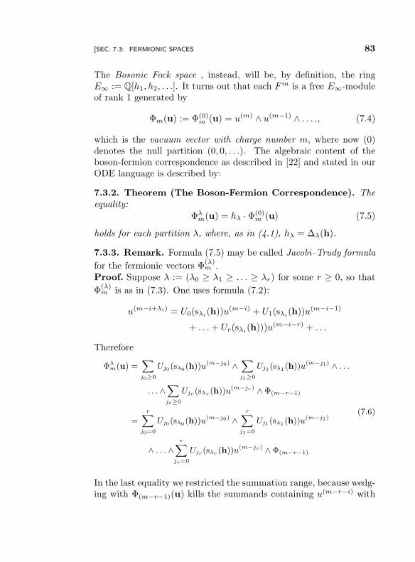
“EscoAlgtot˙New”2012/10/10page 83
i
i
i
i
i
i
i
i
[SEC. 7.3: FERMIONIC SPACES 83
The Bosonic Fock space , instead, will be, by definition, the ringE∞ := Q[h1, h2, . . .]. It turns out that each Fm is a free E∞-moduleof rank 1 generated by
Φm(u) := Φ(0)m (u) = u(m) ∧ u(m−1) ∧ . . . ., (7.4)
which is the vacuum vector with charge number m, where now (0)denotes the null partition (0, 0, . . .). The algebraic content of theboson-fermion correspondence as described in [22] and stated in ourODE language is described by:
7.3.2. Theorem (The Boson-Fermion Correspondence). Theequality:
Φλm(u) = hλ · Φ(0)
m (u) (7.5)
holds for each partition λ, where, as in (4.1), hλ = ∆λ(h).
7.3.3. Remark. Formula (7.5) may be called Jacobi–Trudy formula
for the fermionic vectors Φ(λ)m .
Proof. Suppose λ := (λ0 ≥ λ1 ≥ . . . ≥ λr) for some r ≥ 0, so that
Φ(λ)m is as in (7.3). One uses formula (7.2):
u(m−i+λi) = U0(sλi(h))u(m−i) + U1(sλi
(h))u(m−i−1)
+ . . .+ Ur(sλi(h)))u(m−i−r) + . . .
Therefore
Φλm(u) =
∑
j0≥0
Uj0(sλ0(h))u(m−j0) ∧∑
j1≥0
Uj1(sλ1(h))u(m−j1) ∧ . . .
. . . ∧∑
jr≥0
Ujr (sλr (h))u(m−jr) ∧ Φ(m−r−1)
=r∑
j0=0
Uj0(sλ0(h))u(m−j0) ∧r∑
j1=0
Uj1(sλ1(h))u(m−j1)
∧ . . . ∧r∑
jr=0
Ujr (sλr (h))u(m−jr) ∧ Φ(m−r−1)
(7.6)
In the last equality we restricted the summation range, because wedg-ing with Φ(m−r−1)(u) kills the summands containing u(m−r−i) with
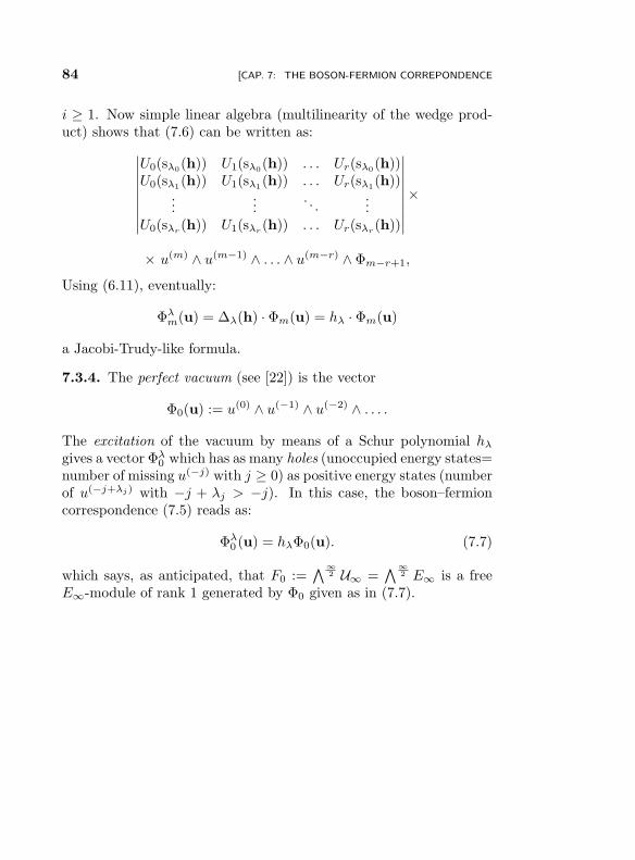
“EscoAlgtot˙New”2012/10/10page 84
i
i
i
i
i
i
i
i
84 [CAP. 7: THE BOSON-FERMION CORREPONDENCE
i ≥ 1. Now simple linear algebra (multilinearity of the wedge prod-uct) shows that (7.6) can be written as:
∣∣∣∣∣∣∣∣∣
U0(sλ0(h)) U1(sλ0
(h)) . . . Ur(sλ0(h))
U0(sλ1(h)) U1(sλ1
(h)) . . . Ur(sλ1(h))
......
. . ....
U0(sλr(h)) U1(sλr
(h)) . . . Ur(sλr(h))
∣∣∣∣∣∣∣∣∣
×
× u(m) ∧ u(m−1) ∧ . . . ∧ u(m−r) ∧ Φm−r+1,
Using (6.11), eventually:
Φλm(u) = ∆λ(h) · Φm(u) = hλ · Φm(u)
a Jacobi-Trudy-like formula.
7.3.4. The perfect vacuum (see [22]) is the vector
Φ0(u) := u(0) ∧ u(−1) ∧ u(−2) ∧ . . . .
The excitation of the vacuum by means of a Schur polynomial hλ
gives a vector Φλ0 which has as many holes (unoccupied energy states=
number of missing u(−j) with j ≥ 0) as positive energy states (numberof u(−j+λj) with −j + λj > −j). In this case, the boson–fermioncorrespondence (7.5) reads as:
Φλ0 (u) = hλΦ0(u). (7.7)
which says, as anticipated, that F0 :=∧∞
2 U∞ =∧∞
2 E∞ is a freeE∞-module of rank 1 generated by Φ0 given as in (7.7).
“EscoAlgtot˙New”2012/10/10page 85
i
i
i
i
i
i
i
i
Bibliography
[1] R. P. Agarwal, Difference Equations and Inequalities, SecondEdition, Marcel Dekker, inc., New York (2000).
[2] T. M. Apostol, Calculus, Vol. II, Second Edition, John Wileyand Sons, New York, 1962.
[3] E. Arbarello, Sketches of KdV, Symposium in Honor of C. H.Clemens (Salt Lake City, UT, 2000), Contemp. Math., 312,Amer. Math. Soc., Providence, RI, 2002, 9–69.
[4] C. Bartocci, G. Falqui, I. Mencattini, G. Ortenzi, M. Pedroni,On the geometric origin of the bi-Hamiltonian structure of the
Calogero-Moser system, Int. Math. Res. Not. IMRN 2010, no. 2,279–296.
[5] R. Camporesi, Linear ordinary differential equations. Revisit-
ing the impulsive response method using factorization, Int. J. ofMath. Education in Sci. and Technology, 42, no. 4, 2011, 497–514.
[6] H. Cartan, Theorie elementaire des fonctions analytiques d’une
ou plusieurs variables complexes, Hermann, Paris, 1961.
[7] C. Carvalho, On V-Weierstrass sets and gaps, J. Algebra 312(2007), no. 2, 956–962.
[8] J. Cordovez, L. Gatto, T. Santiago, Newton binomial formulas
in Schubert calculus, Rev. Mat. Complut. 22 (2009), no. 1, 129–152.
85
“EscoAlgtot˙New”2012/10/10page 86
i
i
i
i
i
i
i
i
86 BIBLIOGRAPHY
[9] S. C. Coutinho, A primer of algebraic D-modules, London Math-ematical Society Student Texts, 33, Cambridge University Press,Cambridge, 1995.
[10] T. Ekedahl, D. Laksov, Splitting Algebras, Symmetric Functions
and Galois Theory, J. Alg. and Appl., 4, no. 1, 2005, 59–75.
[11] W. Fulton, Intersection Theory, Ergebnisse der Mathematik undihrer Grenzgebiete (3), vol. 2, Springer-Verlag, Berlin (1984).
[12] W. Fulton, Young Diagrams, London Mathematical Society Stu-dent Texts, 35, Cambridge University Press, Cambridge (1997).
[13] L. Gatto, Schubert Calculus via Hasse–Schmidt Derivations,Asian J. Math. 9, No. 3, 315–322, (2005).
[14] L. Gatto, Schubert Calculus: An Algebraic Introduction, Pub-licacoes Matematicas do IMPA, 25o Coloquio Brasileiro deMatematica, Instituto Nacional de Matematica Pura e Aplicada(IMPA), Rio de Janeiro, 2005.
[15] L. Gatto, The Wronskian and its Derivatives, Atti Acc. Pelori-tana dei Pericolanti, Physical, Mathematical, and Natural Sci-ences, 89, no. 2 (2011), 14 pages.
[16] L. Gatto, P. Salehyan, Families of Special Weierstrass Points, C.R. Acad. Sci. Paris, Ser. I 347 (2009) 1295–1298.
[17] L. Gatto, T. Santiago, Schubert Calculus on a Grassmann Alge-
bra, Canad. Math. Bull. 52 (2009), no. 2, 200–212.
[18] L. Gatto, I. Scherbak, “On One Property of One Solution of
One Equation” or Linear ODE’s, Wronskians and Schubert Cal-
culus, Moscow Math. J., To the seventy-fifth anniversary ofV. I. Arnold, 12 (2012), No. 2, 275–291.
[19] L. Gatto, I. Scherbak, On Generalized Wronskians, in “Contribu-tions to Algebraic Geometry”. Impanga Lecture Notes”, P. Pra-gacz ed., EMS Series of Congress Reports, 257–296, 2012.
“EscoAlgtot˙New”2012/10/10page 87
i
i
i
i
i
i
i
i
BIBLIOGRAPHY 87
[20] Huang Yong-nian, The Explicit Solution of Homogeneous Lin-
ear Ordinary Differential Equations with Constant Coefficients,Applied Mathematics and Mechanics (English Edition, VoI. 13,No.12, 1115–1120, 1992.
[21] V. G. Kac, Vertex Algebras for Beginners, University LectureSeries, Vol. 10, AMS, 1996.
[22] V. G. Kac, A. K. Raina, Highest Weight Representations of Infi-
nite Dimensional Lie Algebras, Advanced Studies in Mathemat-ical Physics, Vol. 2, World Scientific, 1987.
[23] M. E. Kazarian, S. K. Lando, An algebro-geometric proof of
Witten’s conjecture, J. Amer. Math. Soc. 20 (2007), no. 4, 1079–1089.
[24] D. Laksov, A. Thorup, A Determinantal Formula for the Exte-
rior Powers of the Polynomial Ring, Indiana Univ. Math. J. 56,No. 2 (2007), 825–845.
[25] D. Laksov, A. Thorup, Schubert Calculus on Grassmannians and
Exterior Products, Indiana Univ. Math. J. 58 No. , 2009, 283–300.
[26] S. Lang, Algebra, Third Edition, Addison Wesley, 1993.
[27] E. Liz, A Note on the Matrix Exponential, SIAM Rev., Vol. 40,No. 3, 1998, 700–702.
[28] I. H. Leonard, The Matrix Exponential, SIAM rev., Vol. 38, No.3, 1996, 507–512.
[29] I. G. Macdonald, Symmetric functions and Hall poynomials,Clarendon Press, Oxford, 1979.
[30] M. Mulase, Algebraic theory of the KP equations, Perspec-tives in Mathematical Physics, Conf. Proc. Lecture Notes Math.Phys., III, Int. Press, Cambridge, MA, 151–217, 1994.
[31] Y. A. Neretin, A remark on the boson-fermion correspon-
dence in “Coherent states, differential and quantum geometry”(Bia lowieza, 1997). Rep. Math. Phys. 43 (1999), no. 1-2, 267–269.
“EscoAlgtot˙New”2012/10/10page 88
i
i
i
i
i
i
i
i
88 BIBLIOGRAPHY
[32] M. Pacini, Compactifying moduli of hyperelliptic curves Rend.Circ. Mat. Palermo (2) 56 (2007), no. 2, 157–170.
[33] E. J. Putzer, Avoiding the Jordan canonical form in the discus-
sion of linear systems with constant coefficients, Amer. Math.Monthly 73, 1966, 2–7.
[34] R. Vidal Martins, Trigonal non-Gorenstein curves, J. Pure Appl.Algebra 209 (2007), no. 3, 873–882.
“EscoAlgtot˙New”2012/10/10page 89
i
i
i
i
i
i
i
i
Index
A-algebra, 7D-modules, 33Q-algebras, 18
Mobius band, 37Universal Cauchy formula, 32
Bezout’s theorem, 71bilinear map, 5binomial coefficient, 14boson-fermion correspondence,
80bosonic Fock space, 83
cap product, 70Cayley and Hamilton theorem,
54Chern classes, 71companion matrix, 55, 56cosine, 34
degree of a subvariety of Pn,70
derivation on an exterior alge-bra, 67
exponential formal power se-ries, 20
exterior algebra, 9
fermionic space, 80Fock space, 79formal Laplace transform, 10,
19formal Laurent series, 11formal power series, 9
generalized wronskian, 44generalized Wronskians, 2generating functions, 14Giambelli’s formula, 68
Hadamard’s theorem, 21hook length, 42
impulsive response kernel, 32infinite–order, linear ODE of,
40initial conditions, 30invertible module, 7
Jacobi identity, 8Jacobi-Trudy for Wronskians,
47
length of a partition, 41Lie Algebra, 8linear ODE of infinite order,
81
89
“EscoAlgtot˙New”2012/10/10page 90
i
i
i
i
i
i
i
i
90 INDEX
Littlewood–Richardson coeffi-cients, 49
module of solutions of the ho-mogeneous linear ODE,29
module over a ring, 5
order of a formal Laurent se-ries, 11
Ordinary Differential Operator,27
part of a partition, 41partition, 41permutation, 9Pieri’s formula, 68
rank, 9residue of a formal Laurent se-
ries, 11
Schubert derivation, 67sine, 34
tensor product, 6
universal Cauchy problem, 38Universal Euler formula, 35universal polynomial, 22Universal splitting agebra, 35
weight, 66weight graduation, 66, 67weight of a partition, 41